Scalable Hashing-Based Network DiscoveryTara Safavi

Computer Science and EngineeringUniversity of Michigan

Ann Arbor, MI

Chandra SripadaPsychiatry and Philosophy

University of MichiganAnn Arbor, MI

Danai KoutraComputer Science and Engineering

University of MichiganAnn Arbor, MI

Abstract—Discovering and analyzing networks from non-network data is a task with applications in fields as diverse asneuroscience, genomics, energy, economics, and more. In thesedomains, networks are often constructed out of multiple timeseries by computing measures of association or similarity betweenpairs of series. The nodes in a discovered graph correspond totime series, which are linked via edges weighted by the associationscores of their endpoints. After graph construction, the networkmay be thresholded such that only the edges with strongerweights remain and the desired sparsity level is achieved.

While this approach is feasible for small datasets, its quadratictime complexity does not scale as the individual time serieslength and the number of compared series increase. Thus, toavoid the costly step of building a fully-connected graph beforesparsification, we propose a fast network discovery approachbased on probabilistic hashing of randomly selected time seriessubsequences. Evaluation on real data shows that our methodsconstruct graphs nearly 15 times as fast as baseline methods,while achieving both network structure and accuracy comparableto baselines in task-based evaluation.

I. INTRODUCTION

Prevalent among data in the natural, social, and informationsciences are graphs or networks, which are abstract data struc-tures consisting of entities (nodes) and connections amongthose entities (edges). In some cases, graphs are directlyobserved, as in the well-studied example of social networks,where nodes represent users and edges represent a varietyof user interactions such as friendship, likes, or comments.However, graphs may also be constructed from non-networkdata, a task of interest in domains such as neuroscience [7][11],finance [24], and transportation [29], where practitioners seekto represent similarity or correlation among pairs of timeseries as network interactions in order to gain network-relatedinsights from the resultant graphs.

Motivated by the growing need for scalable data analysis,we address the problem of efficient network discovery on manytime series, which may be informally described as:

Problem 1 (Efficient network discovery: informal). GivenN time series X = x(1), . . . , x(N), efficiently construct asparse similarity graph which captures the strong associations(edges) between the time series (nodes).

Traditional network discovery [7][21] on time series suffersfrom the simple but serious drawback of scalability. Theestablished technique for building a graph out of N time seriesis to compare all pairs of series, forming a fully-connectedgraph where nodes are time series and edges are weighted

Fig. 1: Network discovery: a key to efficiency is to avoid theall-pairs similarity computations.

proportionally to the computed similarity or association ofthe nodes they connect [13], with optional sparsificationafterward to keep only the stronger associations. This all-pairs method is at least an Ω(N2) operation depending onthe complexity of the similarity measure, which makes theprocess computationally inefficient and wasteful on anythingother than small datasets. For example, to generate even asmall graph of 5000 nodes, about 12.5 million comparisonsare required for a graph that may eventually lose most of itsedges via thresholding before further analysis. Moreover, eachcomparison itself is at least linear in the time series length. Forexample, correlation is linear, and the dynamic time warping(DTW) distance measures are slower yet, adding an extraruntime factor as the series length increases.

We propose to circumvent the bottleneck of the establishednetwork discovery approach, namely the all-pairs comparison,by introducing a new method based on locality-sensitive hash-ing (LSH) tailored to time series. Informally, we first computea compact randomized signature for each time series, then hashall series with the same signature to the same “bucket” suchthat only the intra-bucket pairwise similarity scores need becomputed. Our main contributions are as follows:

• Novel distance measure. Constrained by the theoreticalrequirements of LSH and motivated by the widespreaduse of correlation as an association measure, we proposea novel and intuitive time series distance metric, ABC,that captures consecutively matching approximate trendsbetween time series. To the best of our knowledge, thisis the first distance metric to do so.

• Network discovery via hashing. We introduce a new fam-ily of LSH hash functions, window sampling LSH, basedon our proposed distance metric. We show how the falsepositive and negative rates of the randomized hashing

process can be controlled in network construction.• Evaluation on real data. We evaluate the efficiency and

accuracy of our method. To evaluate accuracy, we rely ondomain knowledge from neuroscience, an area of activeresearch on discovered networks. The graphs built byour proposed method, ABC-LSH, are created up to 15×faster than baselines, while performing just as well inclassification-based evaluation.

For reproducibility, we make the code available athttps://github.com/tsafavi/hashing-based-network-discovery.

II. RELATED WORK

Recently there has been significant interest in inferringsparse graphical models from multivariate data using lassoregularization (inverse covariance estimation) [15][30]. Theseapproaches assume that the data follow a k-variate normaldistribution N(0,Σ), where k is the number of the parametersand Σ is the covariance of the distribution. Recent workfocuses on scaling this approach, albeit with the same mod-eling assumptions. In our work, we tackle efficient networkdiscovery without distributional assumptions.

In graph signal processing, “graph signals” are described asfunctions on the nodes in the graph, where high-dimensionaldata represent nodes and weighted edges connect nodes ac-cording to similarity [29]. While graph signal processing in-volves transforming time series signals to construct a weightedsimilarity graph, its focus is more on extending traditionalsignal processing tools to graphs—the filtering and transform-ing of the signals themselves—rather than the efficiency orevaluation of network discovery.

The problem of fast k-nearest neighbor graph constructionhas also been addressed. In a k-NN graph, each node isconnected to the top k most similar other nodes in thegraph. Some methods proposed to improve the quadraticruntime of traditional k-NN graph construction include localsearch algorithms and hashing [12] [31]. However, limitingthe number of neighbors per node is an unintuitive task. Ourmethod does not require a predetermined number of nearestneighbors, but rather lets the hashing process determine whichpairs of nodes are connected. Relatedly, the set similarity self-join problem [8] seeks to identify all pairs of objects abovea user-set similarity threshold. We argue that thresholding isneither intuitive nor informative in network discovery: we seekto analyze the resultant network’s connectivity patterns andstrengths without hard-to-define edge weight thresholds.

Locality-sensitive hashing (LSH) [3] has been successfullyemployed in various settings, including efficiently findingsimilar documents. Unlike general hashing, which aims toavoid collisions between data points, LSH encourages col-lisions between items such that, with high probability, onlycolliding elements are similar. In our domain, general methodsof hashing time series have been proposed, although neither forthe purpose of graph construction nor approximation of corre-lation between two time series [17] [20] [19]. Most recently,random projections of sliding windows on time series havebeen proposed for constructing approximate short signatures

TABLE I: Major symbols.

Symbol Definitionx a time series, or a real-valued length-n sequenceX a set of N time series x(1), . . . , x(N)b(x) binary approximation of a time series xS(x, y) maximum ABC similarity between two sequencesp number of agreeing “runs” between two sequenceski length of the i-th agreeing “run” between two sequencesα The parameter upon which ABC operates; α controls the

emphasis on consecutiveness as a factor in similarity scoringF LSH family of hash functionsk length of a window or subsequence of xr number of hash functions to AND with LSHb number of hash functions to OR with LSH

for hashing [23]. However, this approach uses dynamic timewarping (DTW) as a measure of time series distance. WhileDTW has the advantage of potentially matching similarly-shaped time series out of phase in the time axis, it is not ametric, unlike our proposed measure, and therefore cannot beused for theoretical guarantees of false positives and negativesin hashing [26].

In summary, while fields tangential to our problem havebeen explored, some to a greater degree than others, to thebest of our knowledge efficient network discovery on timeseries with hashing has not been explored.

III. PROPOSED APPROACH

The problem we address is given as:

Problem 2 (Multiple time series to weighted graph). GivenN time series X = x(1), . . . , x(N), construct a similaritygraph where each node corresponds to a time series x(i) andeach edge is weighted according to the similarity of the nodes(x(i), x(j)) that it connects.

As previously stated, the traditional method of networkdiscovery on time series is quadratic in the number of timeseries N , and its total complexity also depends on the chosensimilarity measure. We thus propose a 3-step method, depictedin Figure 2, that avoids the costly all-pairs comparison step:

1) Preprocess time series. First, the input real-valued timeseries are approximated as binary sequences, following arepresentation that captures “trends”.

2) Hash binary sequences to buckets. Next, the binarysequences are hashed to short, randomized signatures.To achieve this, we define a novel distance metric thatis both theoretically eligible for LSH and qualitativelycomparable to the commonly-used correlation measure.

3) Compute intra-bucket pairwise similarity. Each pair oftime series that hash to the same signature, or bucket, arecompared such that an edge is created between them.

The output of the process is a graph in which all pairsof time series that collide in any round of hashing areconnected by an edge weighted according to their similarity.For reference, Table I defines the major symbols we use.

A. Time Series RepresentationThe first step in our pipeline converts raw, real-valued time

series to binary, easily hashable sequences. In the literature,

Fig. 2: Our proposal, ABC-LSH. The output of step 3 is a graph where edges are weighted according to node similarity.

several binarized representations of time series have beenproposed [18] [4] [27]. The one we use has been called the“clipped” representation of a time series [27].

Definition 1 (Binarized representation of time series).Given a time series x ∈ Rn, the binarized representation ofthe series b(x) replaces each real value xi, i ∈ [1, n], by asingle bit such that b(xi) = 1 if xi is above the series meanµx, and 0 otherwise.

We choose this representation because it captures keyfluctuations in the time series—which we want to compare,as correlation does—while approximating the time series ina manner that facilitates fast similarity search. In particular,LSH requires a method of computing hash signatures ofreduced dimensionality from input data, which is dependenton which similarity or distance measure is chosen. In ourproposals, binarizing the time series naturally gives way tothe construction of short, representative hash signatures. Aswe show in the evaluation, these benefits outweigh the “loss”of information from converting to binary: we are able toapproximate correlation well with just 1s and 0s.

B. ABC: Approximate Binary Correlation

Given binary sequences that approximate real-valued timeseries, we propose an intuitive and simple measure of sim-ilarity, and a complementary distance metric, that mirrorstraditional correlation by observing matching consecutive fluc-tuations between pairs of series. The intuition is that captur-ing similarity via pointwise agreement—e.g., via Euclideandistance (ED) or other commonly used measures—can bemisleading or ineffective. Agreement between two series int randomly scattered timesteps may not capture overall simi-larity in trends, whereas two series following the exact samepattern of fluctuations in t consecutive timesteps are arguablymore “associated”. Figure 3 illustrates this with ED and showsthe effectiveness of our proposed measure.

The intuition behind our proposed metric, ABC or Approx-imate Binary Correlation, is to count similar bits between twobinarized time series x and y, while slightly exponentiallyweighting consecutively similar bits in x and y such thatthe longer the consecutive matching subsequences, which wecall runs [5], the more similar x and y will be deemed.More formally, we define the similarity score as a summationof multiple geometric series, which elegantly captures thisintuition. For some 0 < α 1, ABC adds (1+α)i to the total“similarity score” for every i-th consecutive bit of agreementbetween the two series, starting with i = 0 every time a newrun begins. Thus, the similarity of two binarized series is a

Fig. 3: Although time series x and y are more visually similarin (a) than the other pairs, Euclidean distance (ED) and otherpointwise methods fail to reflect that, as x and z are assigned thelowest Euclidean distance (i.e., are the most similar with ED). Bycontrast, our ABC distance metric assigns the lowest distance tox and y. Moreover, it approximates correlation and admits LSH.

sum of 1 ≤ p ≤ n2 geometric series, each with a common ratio

r = (1+α) and a length ki where k1+ . . .+ki+ . . .+kp ≤ n.A visual depiction of computing similarity is given in Figure 4.

The parameter α controls the emphasis on consecutivenessin similarity scoring. For example, choosing α = 0 reduces thesimilarity score to the complement of Hamming distance, andincreasing α both increases the maximum similarity score, asexplained in the next paragraph, and the “gap” between pairsof series that match in long consecutive runs versus shorterruns (for example, agreement in every other timestep).

Definition 2 (ABC: Approximate Binary Correlation).Given two binarized time series x, y ∈ 0, 1n, which havep matching consecutive subsequences i of length ki, the ABCsimilarity is defined as

s(x, y) =

p∑i=1

ki∑b=0

(1 + a)b =

∑pi=1 (1 + α)ki − p

α(III.1)

Fig. 4: The ABC similarity between x and y is the sum of thetwo geometric series that encode the length-2 and 3 runs.

where α ∈ (0, 1] controls the emphasis on consecutiveness:higher α, higher emphasis. Above we use that the sum of ageometric progression is

∑n−1b=0 r

b = 1−rn1−r for r 6= 1.

The maximum possible ABC similarity for two identicalseries, which we denote S(x, y), is the sum of a geometricprogression from 0 to n − 1 with common ratio (1 + α):S(x, y) =

∑n−1i=0 (1 + α)i = (1+α)n−1

α .We derive the complementary distance score by simply

subtracting from the maximum similarity. Thus, identicalsequences will have a distance of 0, and sequences with noagreeing bits will have a distance of S(x, y):

d(x, y) = S(x, y)− s(x, y) =

∑pi=1 (1 + α)ki + p− 1

α(III.2)

To the best of our knowledge, the ABC distance is the firstmetric that goes beyond pointwise comparisons and approxi-mates the widely-used correlation well. As we explain in thefollowing sections, the metric property is key for speeding upthe network discovery problem.

C. Comparison to Correlation

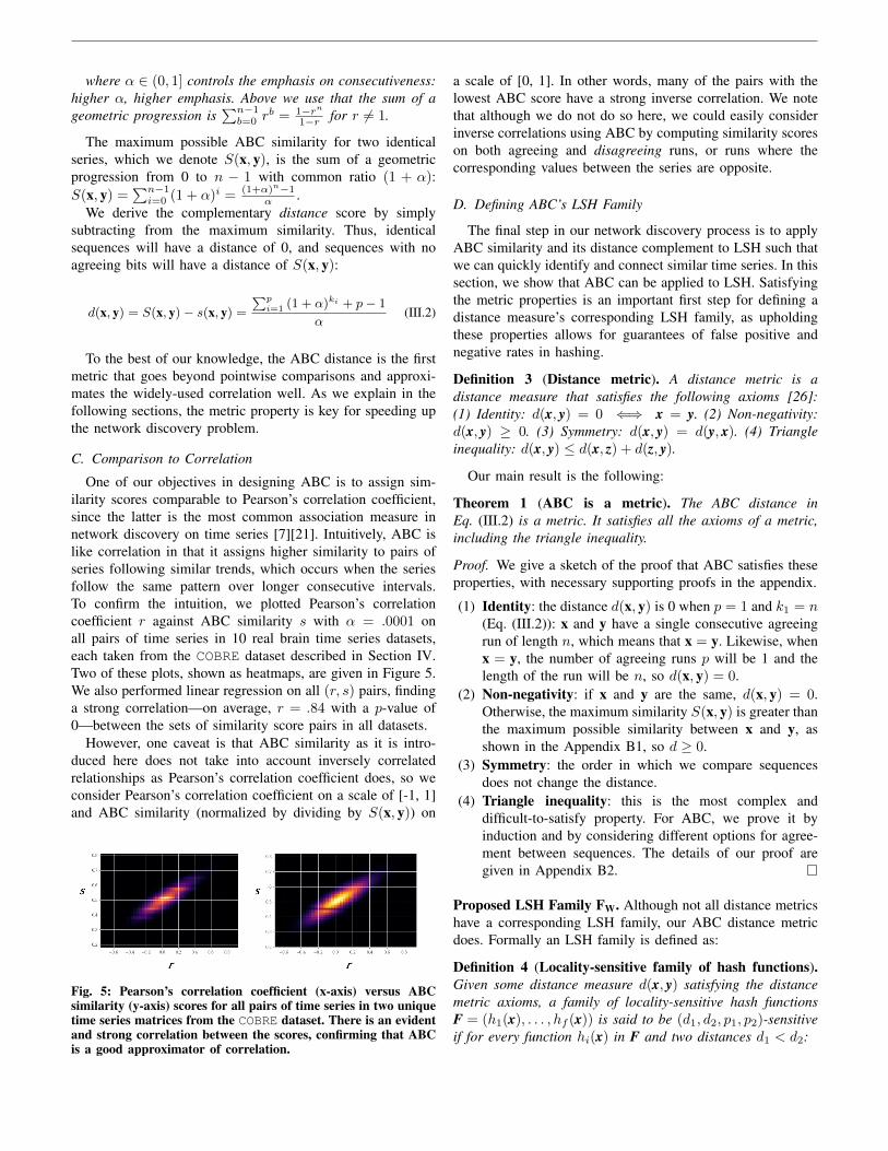
One of our objectives in designing ABC is to assign sim-ilarity scores comparable to Pearson’s correlation coefficient,since the latter is the most common association measure innetwork discovery on time series [7][21]. Intuitively, ABC islike correlation in that it assigns higher similarity to pairs ofseries following similar trends, which occurs when the seriesfollow the same pattern over longer consecutive intervals.To confirm the intuition, we plotted Pearson’s correlationcoefficient r against ABC similarity s with α = .0001 onall pairs of time series in 10 real brain time series datasets,each taken from the COBRE dataset described in Section IV.Two of these plots, shown as heatmaps, are given in Figure 5.We also performed linear regression on all (r, s) pairs, findinga strong correlation—on average, r = .84 with a p-value of0—between the sets of similarity score pairs in all datasets.

However, one caveat is that ABC similarity as it is intro-duced here does not take into account inversely correlatedrelationships as Pearson’s correlation coefficient does, so weconsider Pearson’s correlation coefficient on a scale of [-1, 1]and ABC similarity (normalized by dividing by S(x, y)) on

Fig. 5: Pearson’s correlation coefficient (x-axis) versus ABCsimilarity (y-axis) scores for all pairs of time series in two uniquetime series matrices from the COBRE dataset. There is an evidentand strong correlation between the scores, confirming that ABCis a good approximator of correlation.

a scale of [0, 1]. In other words, many of the pairs with thelowest ABC score have a strong inverse correlation. We notethat although we do not do so here, we could easily considerinverse correlations using ABC by computing similarity scoreson both agreeing and disagreeing runs, or runs where thecorresponding values between the series are opposite.

D. Defining ABC’s LSH Family

The final step in our network discovery process is to applyABC similarity and its distance complement to LSH such thatwe can quickly identify and connect similar time series. In thissection, we show that ABC can be applied to LSH. Satisfyingthe metric properties is an important first step for defining adistance measure’s corresponding LSH family, as upholdingthese properties allows for guarantees of false positive andnegative rates in hashing.

Definition 3 (Distance metric). A distance metric is adistance measure that satisfies the following axioms [26]:(1) Identity: d(x, y) = 0 ⇐⇒ x = y. (2) Non-negativity:d(x, y) ≥ 0. (3) Symmetry: d(x, y) = d(y, x). (4) Triangleinequality: d(x, y) ≤ d(x, z) + d(z, y).

Our main result is the following:

Theorem 1 (ABC is a metric). The ABC distance inEq. (III.2) is a metric. It satisfies all the axioms of a metric,including the triangle inequality.

Proof. We give a sketch of the proof that ABC satisfies theseproperties, with necessary supporting proofs in the appendix.

(1) Identity: the distance d(x, y) is 0 when p = 1 and k1 = n(Eq. (III.2)): x and y have a single consecutive agreeingrun of length n, which means that x = y. Likewise, whenx = y, the number of agreeing runs p will be 1 and thelength of the run will be n, so d(x, y) = 0.

(2) Non-negativity: if x and y are the same, d(x, y) = 0.Otherwise, the maximum similarity S(x, y) is greater thanthe maximum possible similarity between x and y, asshown in the Appendix B1, so d ≥ 0.

(3) Symmetry: the order in which we compare sequencesdoes not change the distance.

(4) Triangle inequality: this is the most complex anddifficult-to-satisfy property. For ABC, we prove it byinduction and by considering different options for agree-ment between sequences. The details of our proof aregiven in Appendix B2.

Proposed LSH Family FW. Although not all distance metricshave a corresponding LSH family, our ABC distance metricdoes. Formally an LSH family is defined as:

Definition 4 (Locality-sensitive family of hash functions).Given some distance measure d(x, y) satisfying the distancemetric axioms, a family of locality-sensitive hash functionsF = (h1(x), . . . , hf (x)) is said to be (d1, d2, p1, p2)-sensitiveif for every function hi(x) in F and two distances d1 < d2:

(1) If d(x, y) ≤ d1, then the probability that hi(x) = hi(y) isat least p1. The higher the p1, the lower the probabilityof false negatives.

(2) If d(x, y) ≥ d2, then the probability that hi(x) = hi(y) isat most p2. The lower the p2, the lower the probabilityof false positives.

The simplest LSH family uses bit sampling [16] and ap-plies to Hamming distance, which quantifies the number ofdiffering components between two vectors. The bit-samplingLSH family FH over n-dimensional binary vectors consists ofall functions that randomly select one of its n components orbits: FH = h : 0, 1n → 0, 1|h(x) = xi for i ∈ [1, n].Under this family, hi(x) = hi(y) if and only if xi = yi,or in other words the bit at the i-th index of x is thesame as the bit at the i-th index of y. The FH family isa (d1, d2, 1 − d1

n , 1 −d2n )-sensitive family, based on Def. 4.

In this definition, p1 describes the probability of two vectorscolliding when their distance is at most d1 (i.e., x and y differin at most d1 bits). Thus, p1 corresponds to the complementof the probability of the vectors not colliding or, equivalently,the probability of selecting one of the disagreeing bits out ofthe n total bits, d1n . p1 = 1− d1

n ; p2 is derived similarly.We propose a new LSH family, FW, which carries the con-

secutiveness intuition behind ABC. While the established LSHfamily on Hamming distance samples bits, our proposed LSHfamily FW extends this by consisting of randomly sampledconsecutive subsequences, starting from the same index, forall binary sequences in the dataset. An example of how itworks in practice is given in Figure 6.Theorem 2 (Window sampling LSH family). Given awindow size k, our proposed family of hash functions FWconsists of n− k + 1 hash functions:

FW = h : 0, 1n → 0, 1k|h(x) = (xi, . . . , xi+k−1), i ∈ [1, n−k+1]

Equivalently, hi(x) = hi(y) if and only if (xi, . . . , xi+k−1) =(yi, . . . , yi+k−1). The family FW is (d1, d2, 1−α d1

(1+α)n−1 , 1−α d2

(1+α)n−1 )-sensitive.

Proof. Let s1 = S(x, y)−d1 be the complementary similarityscore for d1 and s2 be the complementary similarity score ford2. The probabilities p1 and p2 are derived by scaling d1 andd2 and taking their complement; in other words, they are foundin the same way that Hamming distance is converted into anormalized similarity score for its corresponding LSH family.In our case, if we normalize both d1 and d2 by dividing by themaximum distance S(x, y) we get S(x,y)−s1

S(x,y) and S(x,y)−s2S(x,y) , or

equivalently p1 = s1S(x,y) = α s1

(1+α)n−1 and p2 = α s2(1+α)n−1 .

E. ABC-LSH: Hashing Process for ABC

Given an LSH family, it is typical to construct new “ampli-fied” families F' by the AND and OR constructions of F [26],which provide control of the false positive and negative ratesin the hashing process. Concretely:

Definition 5 (AND and OR Construction). Given a(d1, d2, p1, p2)-sensitive family of LSH functions F =

Fig. 6: The hash function g ANDs the second and fourth hashfunctions (h2 and h4) in the LSH family FW with k = 2, so thehash signatures are the concatenation (i.e. the AND) of the length-2 windows starting from bits two and four of each sequence.

(h1(x), . . . , hf (x)), the AND construction creates a new hashfunction g(x) as a logical AND of r members of F such thatg(x) = hir for each i chosen uniformly at random withoutreplacement from [1, f ]. Then we say g(x) = g(y) if and onlyif hi(x) = hi(y) for all i ∈ [1, r]. The OR construction doesessentially the same as the AND operation, except we say thatg(x) = g(y) if hi(x) = hi(y) for any i ∈ [1, b].

The AND operation turns any locality-sensitive family Finto a new (d1, d2, p1

r, p2r)-sensitive family F', whereas the

OR operation turns the same family F into a (d1, d2, 1− (1−p1)b, 1−(1−p2)b)-sensitive family. To leverage the benefits ofthese constructions, we incorporate both of them in the hashingprocess of our proposed network discovery approach. Let k bethe length of the sampled window, and r, b the number of hashfunctions used in the AND and OR operations, respectively.

AND operation. For the AND operation, we have a singlehash table and a hash function g(x) = hir, where each hiis chosen uniformly at random from FW. We compute a hashsignature for each data point x(i) as a concatenation of the rlength-k potentially overlapping windows starting at index ifor all hi ∈ g. The algorithm returns all of the buckets of thesingle hash table created so that all pairs within each bucketcan be compared. An example round of hashing with the ANDconstruction is depicted in Figure 6.

OR operation. For the OR operation, we create b hash tables.In b rounds, we compute a hash signature for each data point,where the signature is a length-k window starting at index i forsome hi ∈ FW chosen independently and randomly at uniform.Thus each data point is hashed b times, and the algorithmreturns the union of all buckets for the b hash tables such thatall pairs within all buckets can be compared.Parameter Setting. As we show in the experiments, parametersetting is quite intuitive based on the desired properties ofthe constructed graph. Adjusting the parameters controls falsepositive and negative rates. The higher the r, the lower theprobability of false positives; the higher the b, the lowerthe probability of false negatives. The union of AND/ORconstructions form an S-curve, which is explained in moredetail in [26]. In all cases—AND, OR, both, or neither—allpairs (x(i), x(j)) that hash to the same bucket in any of theconstructed tables are compared pairwise, and an edge between(x(i), x(j)) with the computed similarity between the two se-quences is added to the graph G. Notably, the independence ofboth the intra-bucket comparison step and the OR construction

make our algorithm easily and embarrassingly parallelizable,although we do not explore parallelization here.

There are no strict runtime guarantees we can make withLSH, since every series could hash to a unique bucket or thesame bucket depending on the nature of the data. However,while in theory graph construction could be quadratic if alltime series are nearly identical, in practice most datasets—even those with series that are on average correlated—willresult in sub-quadratic graph construction time, as we show inthe experiments.

F. Network Discovery: Putting Everything Together

Having introduced a new distance metric and its correspond-ing LSH family with the necessary theoretical background, weturn back to our original goal: scalable network discovery, asdepicted at a high level in Figure 2. Given N time series,each of length n, we convert all data to binary followingthe representation in Section III-A, then follow the steps inAlgorithm 1, using LSH as described in Section III-E.

Algorithm 1: Window LSH to graphInput : A set of N binarized time series X;

k: length of the window to sample;r: # of windows per time series signature;b: # of hash tables to construct

Output: A weighted graph G = (V,E) where each nodex(i) ∈ V is a time series and each edge(x(i), x(j)) ∈ E has weight s(x(i), x(j))

1 G← GRAPH2 buckets← LSH-AND(X, k, r) ∪ LSH-OR(X, k, b)3 for bucket ∈ buckets do4 for (x(i),x(j)) ∈ bucket do5 weight← S(x(i), x(j))

6 G.ADDEDGE(x(i), x(j), weight)7 end8 end9 return G

IV. EVALUATION

In our evaluation, we strive to answer the following ques-tions by applying our method to several real and syntheticdatasets: (1) How efficient is our approach and how does itcompare to baseline approaches? (2) How do our output graphsperform in real applications, such as classification of patientand healthy brains? (3) How do the network discovery runtimeand network properties change for varying parameters of ABC-LSH? We answer the first two questions in the followingsubsections and the last in Appendix A.

A. Data

We used several datasets from different domains, sincenetwork discovery is relevant in a variety of settings.

Brain data. In recent years, psychiatric and imaging neuro-science have shifted away from the study of segregated or lo-calized brain functions toward a dynamic network perspectiveof the brain, where statistical dependencies and correlationsbetween activity in brain regions can be modeled as a graph

[14]. One well-known data collection procedure from whichthe brain’s network organization may be modeled is resting-state fMRI, which tracks temporal and spatial oscillations ofactivity in neuronal ensembles [25]. Key objectives of resting-state fMRI are to elucidate the network mechanisms of mentaldisorders and to identify diagnostic biomarkers—objective,quantifiable characteristics that predict the presence of adisorder—from brain imaging scans [6]. Indeed, a fundamentalhypothesis in the science of functional connectivity is thatcognitive dysfunction can be illustrated and/or explained bya disturbed functional organization.

For our evaluation of brain graphs, we used two publiclyavailable datasets, given in Table II.

TABLE II: Brain data.

Dataset Description Labeled?COBRE [2] Resting-state fMRI from 147 subjects: 72

patients with schizophrenia and 75 healthycontrols. Each subject is associated with1166 time series (brain regions) measured foraround 100 timesteps, with some variation.For those pairs of time series with unequallengths, we take the minimum of the lengths.

4Controlvs.Patient

Penn[1][28]

Resting-state fMRI from 519 subjects. Eachsubject’s is associated with 3789 time seriesmeasured across 110 timesteps.

8

Both datasets were subject to a standard preprocessingpipeline, including 1) linear detrending, or removal of low-fre-quency signal drift; 2) removal of nuisance effects by regres-sion; 3) band-pass filtering, or rejection of frequencies out ofa certain range; and 4) censoring or removal of timesteps withhigh framewise motion.

For all graphs constructed with pairwise comparison, weheld θ = 0.6. For those graphs constructed with ABC, weheld α = .0001. We constructed graphs with the all-pairsmethod for COBRE and Penn using the absolute value ofPearson’s correlation coefficient as our baseline, as is typicalin functional connectivity studies [14]. We also constructedgraphs on the same datasets using ABC for both the all-pairsand LSH construction methods. For LSH, we set the windowsize k = 10, following a rule of thumb of keeping the windowsize roughly

√n. We set d1 = 10 and d2 = 95, the number of

OR constructions b = 8, and did not use the AND construction(i.e., r = 1) such that we achieved p1 = .9999 and p2 = .36 soas to avoid false negatives for the purpose of comprehensivenearest-neighbors search: we were guaranteed with a 99.99%probability that the ABC distance between any colliding seriesx and y was less than or equal to 10 (out of on average length-100 series).

We acknowledge that our brain datasets are relatively small,as most studies in functional connectivity have used smalldatasets. Therefore, to compare scalability on larger datasets—both in terms of more time series and longer time series—westudied graph construction on a generated synthetic dataset aswell as a real dataset taken from the UCR Time Series archive.

Synthetic data. Synth-Penn consists of 20,000 length-100 time series that were either taken directly from a singlebrain in the Penn dataset or else were randomly selected

phase-shifted versions of time series for the same brainin the Penn dataset. The average absolute correlation inSynth-Penn was |r| = .22. We used the same LSHparameters as with the real brain graphs. For the purpose ofevaluating scalability as the number of time series grows, wegenerated graphs out of the first 1000, 2000, 5000, and 10,000series before using the full dataset.

Star Light Data. We also used the StarLightCurvesdataset, which is the largest time series dataset from the UCRTime Series archive. It comprises 9236 time series each oflength 1024 [9], with an average absolute correlation of |r| =.577. Again, for the purpose of evaluating scalability as thenumber of time series grows, we constructed graphs out ofthe first 1000, 2000, and 5000 time series as well as the fulldataset. For LSH, we set k = 64, d1 = 64, and d2 = 960.Then, to avoid both false positives and false negatives with ahigh probability—and to construct sparser graphs, since ourparameter setting for the brain graphs admitted false positivesat a higher rate—we chose r = 6, and b = 2 for false positiveand negative rates of less than .01. For detailed discussion onparameter tuning of ABC-LSH (r, b, k), we refer the readerto Appendix A.

B. Scalability Analysis

We ran all experiments and evaluation on a single UbuntuLinux server with 12 processors and 256 GB of RAM, writtenin single-threaded Python 3.

Brain data. An overview of the overall graph constructionruntime for all subjects in the COBRE and Penn datasets isgiven in Table III. Since LSH is randomized, we averagedruntimes for LSH-generated graphs over three trials. We findthat though these data are relatively small, meaning that all-pairs comparison is not particularly costly, graph generationwith LSH was still an order of magnitude faster. For example,generating all Penn graphs took over 36 hours (on average, 5minutes/graph) with the pairwise technique, whereas generat-ing the same subject brains with LSH took around 5.5 hours(on average, 38 seconds/graph).

TABLE III: Runtime comparison between pairwise correlationand ABC-LSH for the two brain datasets.

Dataset Pairwise (sec) LSH (sec)COBRE 3,969 441Penn 131,307 19,722

Synthetic data. The differences in graph construction run-time grew more pronounced as the size of the data increased.For example, with N = 20, 000, pairwise construction for asingle graph took over 3 hours, whereas LSH construction tookon average 13 minutes, as shown in Figure 7a.

Star Light Data. While LSH is still faster than pairwisecomparison on the StarLightCurves dataset, we find thatit is in general slower than with the brain data. This result isnot surprising: the number of comparisons performed by LSHdepends heavily on the nature of the data and the averagesimilarity of points in the dataset. The average correlationbetween time series in StarLightCurves is much higher

(a) Synth-Penn data

(b) StarLightCurves dataFig. 7: ABC-LSH vs. pairwise correlation: average runtime w.r.t.the number of nodes. ABC-LSH is up to 14.5× faster. Runtime,plotted on the y-axes, is in log scale.

than that of Synth-Penn, and as such more time series hashto the same bucket. Overall, though, it still outperforms all-pairs comparison at 2− 4× faster, as shown in Figure 7b.

C. Evaluation of Output Graphs

Our goal is not only to scale the process of network discov-ery but to construct graphs that are as useful to practitionersas the traditional pairwise-built graphs. For evaluation, we fo-cused on the brain data, as the neuroscience and neuroimagingcommunities are rich with functional connectivity studies onbrain graphs discovered from resting-state fMRI.

Qualitative analysis. Two properties that are often studiedin constructed functional networks are the graph clusteringcoefficients and average path lengths [10], which are hypothe-sized to encode physical meaning on communication betweenbrain regions. We computed these statistics on all output braingraphs for the COBRE and Penn datasets generated by thepairwise correlation, pairwise ABC, and ABC-LSH methods,and plotted the averages and standard deviations per datasetand method in Figure 8. We find that the averages for bothABC pairwise and ABC-LSH are good approximations of thepairwise correlation baseline.

Task-based evaluation. Since we do not have ground-truth networks for our datasets, we evaluated the qualityand distinguishability of the constructed brain networks byperforming classification on the output COBRE brain graphs,for which we have healthy/schizophrenic labels. We use graphproperties commonly computed on functional networks asfeatures [7]: each output graph is represented by a featurevector of [density, average weighted degree, average clusteringcoefficient, modularity, average path length]T .

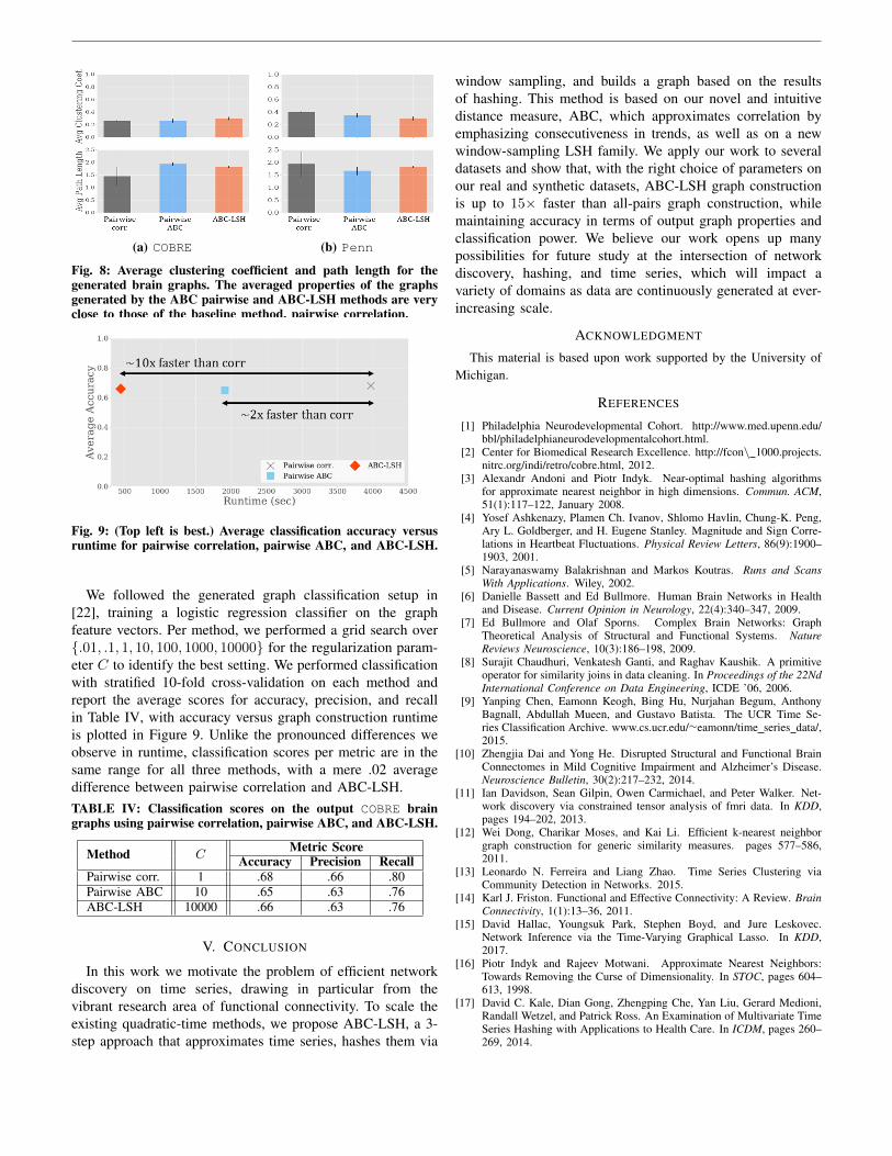
(a) COBRE (b) Penn

Fig. 8: Average clustering coefficient and path length for thegenerated brain graphs. The averaged properties of the graphsgenerated by the ABC pairwise and ABC-LSH methods are veryclose to those of the baseline method, pairwise correlation.

Fig. 9: (Top left is best.) Average classification accuracy versusruntime for pairwise correlation, pairwise ABC, and ABC-LSH.

We followed the generated graph classification setup in[22], training a logistic regression classifier on the graphfeature vectors. Per method, we performed a grid search over.01, .1, 1, 10, 100, 1000, 10000 for the regularization param-eter C to identify the best setting. We performed classificationwith stratified 10-fold cross-validation on each method andreport the average scores for accuracy, precision, and recallin Table IV, with accuracy versus graph construction runtimeis plotted in Figure 9. Unlike the pronounced differences weobserve in runtime, classification scores per metric are in thesame range for all three methods, with a mere .02 averagedifference between pairwise correlation and ABC-LSH.TABLE IV: Classification scores on the output COBRE braingraphs using pairwise correlation, pairwise ABC, and ABC-LSH.

Method CMetric Score

Accuracy Precision RecallPairwise corr. 1 .68 .66 .80Pairwise ABC 10 .65 .63 .76ABC-LSH 10000 .66 .63 .76

V. CONCLUSION

In this work we motivate the problem of efficient networkdiscovery on time series, drawing in particular from thevibrant research area of functional connectivity. To scale theexisting quadratic-time methods, we propose ABC-LSH, a 3-step approach that approximates time series, hashes them via

window sampling, and builds a graph based on the resultsof hashing. This method is based on our novel and intuitivedistance measure, ABC, which approximates correlation byemphasizing consecutiveness in trends, as well as on a newwindow-sampling LSH family. We apply our work to severaldatasets and show that, with the right choice of parameters onour real and synthetic datasets, ABC-LSH graph constructionis up to 15× faster than all-pairs graph construction, whilemaintaining accuracy in terms of output graph properties andclassification power. We believe our work opens up manypossibilities for future study at the intersection of networkdiscovery, hashing, and time series, which will impact avariety of domains as data are continuously generated at ever-increasing scale.

ACKNOWLEDGMENT

This material is based upon work supported by the University ofMichigan.

REFERENCES

[1] Philadelphia Neurodevelopmental Cohort. http://www.med.upenn.edu/bbl/philadelphianeurodevelopmentalcohort.html.

[2] Center for Biomedical Research Excellence. http://fcon\ 1000.projects.nitrc.org/indi/retro/cobre.html, 2012.

[3] Alexandr Andoni and Piotr Indyk. Near-optimal hashing algorithmsfor approximate nearest neighbor in high dimensions. Commun. ACM,51(1):117–122, January 2008.

[4] Yosef Ashkenazy, Plamen Ch. Ivanov, Shlomo Havlin, Chung-K. Peng,Ary L. Goldberger, and H. Eugene Stanley. Magnitude and Sign Corre-lations in Heartbeat Fluctuations. Physical Review Letters, 86(9):1900–1903, 2001.

[5] Narayanaswamy Balakrishnan and Markos Koutras. Runs and ScansWith Applications. Wiley, 2002.

[6] Danielle Bassett and Ed Bullmore. Human Brain Networks in Healthand Disease. Current Opinion in Neurology, 22(4):340–347, 2009.

[7] Ed Bullmore and Olaf Sporns. Complex Brain Networks: GraphTheoretical Analysis of Structural and Functional Systems. NatureReviews Neuroscience, 10(3):186–198, 2009.

[8] Surajit Chaudhuri, Venkatesh Ganti, and Raghav Kaushik. A primitiveoperator for similarity joins in data cleaning. In Proceedings of the 22NdInternational Conference on Data Engineering, ICDE ’06, 2006.

[9] Yanping Chen, Eamonn Keogh, Bing Hu, Nurjahan Begum, AnthonyBagnall, Abdullah Mueen, and Gustavo Batista. The UCR Time Se-ries Classification Archive. www.cs.ucr.edu/∼eamonn/time series data/,2015.

[10] Zhengjia Dai and Yong He. Disrupted Structural and Functional BrainConnectomes in Mild Cognitive Impairment and Alzheimer’s Disease.Neuroscience Bulletin, 30(2):217–232, 2014.

[11] Ian Davidson, Sean Gilpin, Owen Carmichael, and Peter Walker. Net-work discovery via constrained tensor analysis of fmri data. In KDD,pages 194–202, 2013.

[12] Wei Dong, Charikar Moses, and Kai Li. Efficient k-nearest neighborgraph construction for generic similarity measures. pages 577–586,2011.

[13] Leonardo N. Ferreira and Liang Zhao. Time Series Clustering viaCommunity Detection in Networks. 2015.

[14] Karl J. Friston. Functional and Effective Connectivity: A Review. BrainConnectivity, 1(1):13–36, 2011.

[15] David Hallac, Youngsuk Park, Stephen Boyd, and Jure Leskovec.Network Inference via the Time-Varying Graphical Lasso. In KDD,2017.

[16] Piotr Indyk and Rajeev Motwani. Approximate Nearest Neighbors:Towards Removing the Curse of Dimensionality. In STOC, pages 604–613, 1998.

[17] David C. Kale, Dian Gong, Zhengping Che, Yan Liu, Gerard Medioni,Randall Wetzel, and Patrick Ross. An Examination of Multivariate TimeSeries Hashing with Applications to Health Care. In ICDM, pages 260–269, 2014.

[18] Eamonn Keogh and Michael Pazzani. An Indexing Scheme for FastSimilarity Search in Large Time Series Databases. In SSDM, pages56–, 1999.

[19] Yongwook Bryce Kim and Una-May Hemberg, Erik O’Reilly. StratifiedLocality-Sensitive Hashing for Accelerated Physiological Time SeriesRetrieval. In EMBC, 2016.

[20] Yongwook Bryce Kim and Una-May O’Reilly. Large-Scale Physio-logical Waveform Retrieval Via Locality-Sensitive Hashing. In EMBC,pages 5829–5833, 2015.

[21] Chia-Tung Kuo, Xiang Wang, Peter Walker, Owen Carmichael, JiepingYe, and Ian Davidson. Unified and Contrasting Cuts in Multiple Graphs:Application to Medical Imaging Segmentation. In KDD, pages 617–626,2015.

[22] John Boaz Lee, Xiangnan Kong, Yihan Bao, and Constance Moore.Identifying Deep Contrasting Networks from Time Series Data: Appli-cation to Brain Network Analysis. 2017.

[23] Chen Luo and Anshumali Shrivastava. SSH (Sketch, Shingle, and Hash)for Indexing Massive-Scale Time Series. In NIPS Time Series Workshop,2016.

[24] Jukka-Pekka Onnela, Kimmo Kaski, and Jnos Kertsz. Clusteringand Information in Correlation Based Financial Networks. EuropeanPhysical Journal B, 38:353–362, 2004.

[25] Hae-Jeong Park and Karl Friston. Structural and Functional BrainNetworks: From Connections to Cognition. Science, 342(6158), 2013.

[26] Anand Rajaraman and Jeffrey David Ullman. Mining of MassiveDatasets. Cambridge University Press, New York, NY, USA, 2011.

[27] Chotirat Ratanamahatana, Eamonn Keogh, Anthony J. Bagnall, andStefano Lonardi. A Novel Bit Level Time Series Representation withImplication of Similarity Search and Clustering. In PAKDD, pages 771–777, 2005.

[28] T.D. Satterthwaite, M.A. Elliott, K Ruparel, J. Loughead, K. Prab-hakaran, M.E. Calkins, R. Hopson, C. Jackson, J. Keefe, M. Riley, F.D.Mentch, P. Sleiman, R. Verma, C. Davatzikos, H. Hakonarson, R.C. Gur,and R.E. Gur. Neuroimaging of the Philadelphia NeurodevelopmentalCohort. NeuroImage, 86:544–553, 2014.

[29] D. I. Shuman, S. K. Narang, P. Frossard, A. Ortega, and P. Van-dergheynst. The emerging field of signal processing on graphs: Ex-tending high-dimensional data analysis to networks and other irregulardomains. IEEE Signal Processing Magazine, 30(3):83–98, 2013.

[30] Sen Yang, Qian Sun, Shuiwang Ji, Peter Wonka, Ian Davidson, andJieping Ye. Structural graphical lasso for learning mouse brain connec-tivity. In KDD, pages 1385–1394, 2015.

[31] Yan-Ming Zhang, Kaizhu Huang, Guanggang Geng, and Cheng-Lin Liu.Fast knn graph construction with locality sensitive hashing. In ECMLPKDD, pages 660–674, 2013.

APPENDIX

A. Appendix 1: Sensitivity Analysis of ABC-LSH

Runtime. Since the number of time series compared in ABC-LSH depends on the length of hash signatures r, the numberof hash tables constructed b, and the window length k, wegenerated a single brain graph from a COBRE subject with avariety of LSH settings using ABC-LSH and α = .0001:

1) r ∈ [1, 5], holding b = 4 and k = 3;2) b ∈ [1, 5], holding r = 2 and k = 3;3) k ∈ [3, 5], holding r = 2 and b = 4;

The runtime trends are plotted in Figure 10. As expected,increasing r and/or k reduced graph construction runtime,

(a) Increasing r. (b) Increasing b. (c) Increasing k.

Fig. 10: ABC-LSH graph construction time vs. parameters.

(a) Varying r. (b) Varying b. (c) Varying k.

Fig. 11: Clustering coeff. and avg. path length for varying theABC-LSH parameters r, b, and k on a single COBRE subject.

whereas increasing b increased graph construction runtime. Forr: the longer the length of the hash signature, the more unlikelythat two time series x and y will have the same signature, soruntime decreases as r increases. For b: the more hash tablescreated, the more “chances” two time series x(i) and x(j) get tocollide, so runtime increases as b increases. For k: the longerthe window length, the more unlikely that two time serieswindows (xi, . . . , xi+k−1) and (yi, . . . , yi+k−1) will matchexactly, so runtime decreases as k increases.Network Properties. As we mentioned earlier, two propertiesthat are often studied in functional networks are the clusteringcoefficient and average path length [10]. We computed thedifferences in these properties among the generated graphs byvarying the parameters of ABC-LSH as before. The changesin properties as the parameters vary are plotted in Figure 11.The trends for average clustering coefficient and average pathlength are quite stable: barring small fluctuations, the averagepath lengths stay short (< 2.5) and the average clusteringcoefficients hover around .4 - .6. These network propertiesof the ABC-LSH networks are robust to parameter changes.

B. Appendix 2: Metric Proof of ABC

Here we give the theoretical foundation that underlies ourtime series distance proposal, ABC. We show that it satisfiesthe metric properties and is thus eligible for LSH.

1) Properties of Agreeing Runs: We first study the relation-ship between p, the number of agreeing runs between x andy, and the maximum value of k1 + . . .+kp, the lengths of thep agreeing runs.

Lemma 1 (Maximum sum of lengths of p runs k1, . . . , kp).Given x, y ∈ 0, 1n with p agreeing runs, each of length ki,the maximum sum of their lengths follows a linearly decreasingrelationship, as

∑pi=1 ki = n− p+ 1.

This follows because the greater the number of runs, themore bits that must “disagree” in order to separate those runs.

Lemma 2 (Maximum ABC similarity). Given x, y ∈ 0, 1nwith p agreeing runs, each of length ki, x and y have maximumABC similarity when they agree on (without loss of generality,the first) p − 1 runs of length k1 = . . . = kp−1 = 1 and onerun of length kp = n− 2p+ 2.

Proof. By induction on p. We omit the proof for brevity.

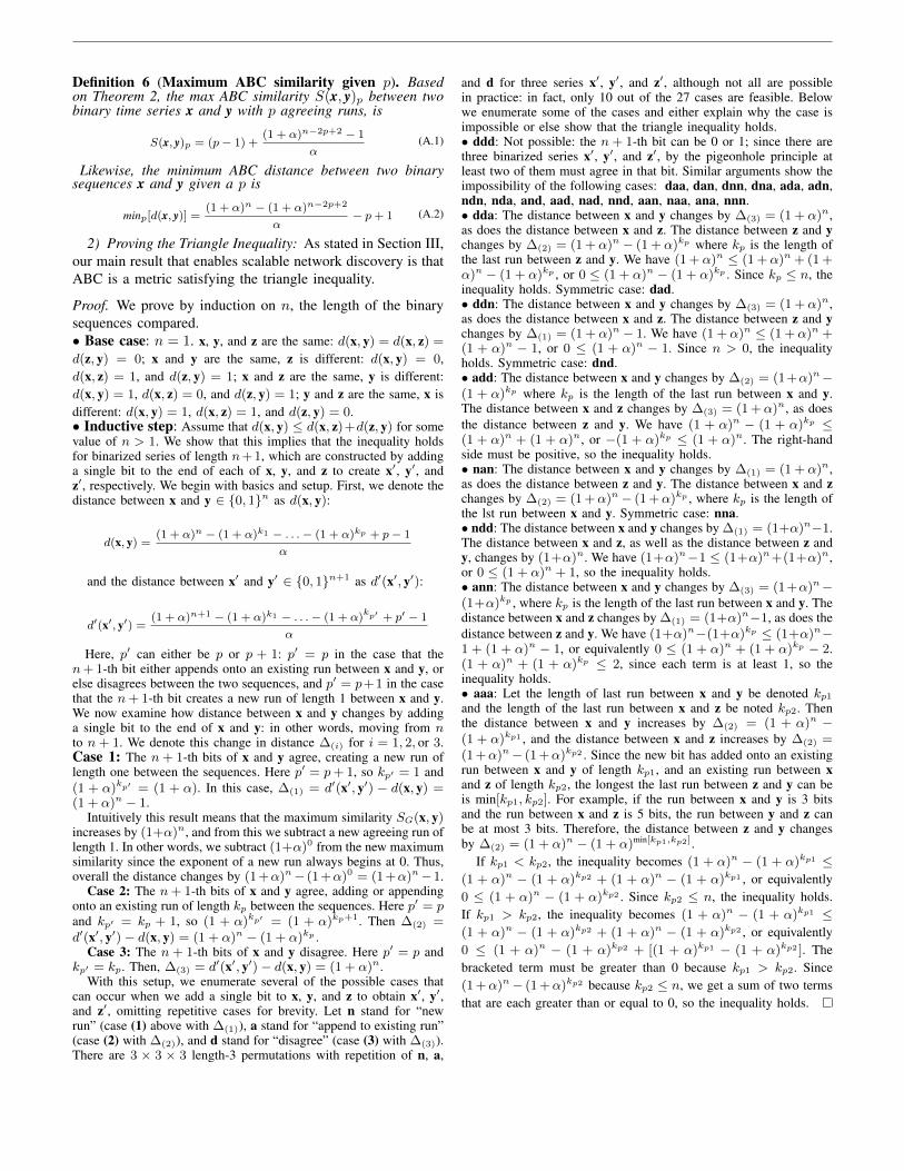
Definition 6 (Maximum ABC similarity given p). Basedon Theorem 2, the max ABC similarity S(x, y)p between twobinary time series x and y with p agreeing runs, is

S(x, y)p = (p− 1) +(1 + α)n−2p+2 − 1

α(A.1)

Likewise, the minimum ABC distance between two binarysequences x and y given a p is

minp[d(x, y)] =(1 + α)n − (1 + α)n−2p+2

α− p+ 1 (A.2)

2) Proving the Triangle Inequality: As stated in Section III,our main result that enables scalable network discovery is thatABC is a metric satisfying the triangle inequality.

Proof. We prove by induction on n, the length of the binarysequences compared.• Base case: n = 1. x, y, and z are the same: d(x, y) = d(x, z) =

d(z, y) = 0; x and y are the same, z is different: d(x, y) = 0,d(x, z) = 1, and d(z, y) = 1; x and z are the same, y is different:d(x, y) = 1, d(x, z) = 0, and d(z, y) = 1; y and z are the same, x isdifferent: d(x, y) = 1, d(x, z) = 1, and d(z, y) = 0.• Inductive step: Assume that d(x, y) ≤ d(x, z)+d(z, y) for somevalue of n > 1. We show that this implies that the inequality holdsfor binarized series of length n+1, which are constructed by addinga single bit to the end of each of x, y, and z to create x′, y′, andz′, respectively. We begin with basics and setup. First, we denote thedistance between x and y ∈ 0, 1n as d(x, y):

d(x, y) =(1 + α)n − (1 + α)k1 − . . .− (1 + α)kp + p− 1

α

and the distance between x′ and y′ ∈ 0, 1n+1 as d′(x′, y′):

d′(x′, y′) =(1 + α)n+1 − (1 + α)k1 − . . .− (1 + α)

kp′ + p′ − 1

α

Here, p′ can either be p or p + 1: p′ = p in the case that then+ 1-th bit either appends onto an existing run between x and y, orelse disagrees between the two sequences, and p′ = p+1 in the casethat the n+ 1-th bit creates a new run of length 1 between x and y.We now examine how distance between x and y changes by addinga single bit to the end of x and y: in other words, moving from nto n+ 1. We denote this change in distance ∆(i) for i = 1, 2, or 3.Case 1: The n+ 1-th bits of x and y agree, creating a new run oflength one between the sequences. Here p′ = p+ 1, so kp′ = 1 and(1 + α)kp′ = (1 + α). In this case, ∆(1) = d′(x′, y′) − d(x, y) =(1 + α)n − 1.

Intuitively this result means that the maximum similarity SG(x, y)increases by (1+α)n, and from this we subtract a new agreeing run oflength 1. In other words, we subtract (1+α)0 from the new maximumsimilarity since the exponent of a new run always begins at 0. Thus,overall the distance changes by (1+α)n− (1+α)0 = (1+α)n−1.

Case 2: The n+ 1-th bits of x and y agree, adding or appendingonto an existing run of length kp between the sequences. Here p′ = pand kp′ = kp + 1, so (1 + α)kp′ = (1 + α)kp+1. Then ∆(2) =d′(x′, y′)− d(x, y) = (1 + α)n − (1 + α)kp .

Case 3: The n + 1-th bits of x and y disagree. Here p′ = p andkp′ = kp. Then, ∆(3) = d′(x′, y′)− d(x, y) = (1 + α)n.

With this setup, we enumerate several of the possible cases thatcan occur when we add a single bit to x, y, and z to obtain x′, y′,and z′, omitting repetitive cases for brevity. Let n stand for “newrun” (case (1) above with ∆(1)), a stand for “append to existing run”(case (2) with ∆(2)), and d stand for “disagree” (case (3) with ∆(3)).There are 3 × 3 × 3 length-3 permutations with repetition of n, a,

and d for three series x′, y′, and z′, although not all are possiblein practice: in fact, only 10 out of the 27 cases are feasible. Belowwe enumerate some of the cases and either explain why the case isimpossible or else show that the triangle inequality holds.• ddd: Not possible: the n+ 1-th bit can be 0 or 1; since there arethree binarized series x′, y′, and z′, by the pigeonhole principle atleast two of them must agree in that bit. Similar arguments show theimpossibility of the following cases: daa, dan, dnn, dna, ada, adn,ndn, nda, and, aad, nad, nnd, aan, naa, ana, nnn.• dda: The distance between x and y changes by ∆(3) = (1 + α)n,as does the distance between x and z. The distance between z and ychanges by ∆(2) = (1 + α)n − (1 + α)kp where kp is the length ofthe last run between z and y. We have (1 +α)n ≤ (1 +α)n + (1 +α)n − (1 + α)kp , or 0 ≤ (1 + α)n − (1 + α)kp . Since kp ≤ n, theinequality holds. Symmetric case: dad.• ddn: The distance between x and y changes by ∆(3) = (1 + α)n,as does the distance between x and z. The distance between z and ychanges by ∆(1) = (1 + α)n − 1. We have (1 + α)n ≤ (1 + α)n +(1 + α)n − 1, or 0 ≤ (1 + α)n − 1. Since n > 0, the inequalityholds. Symmetric case: dnd.• add: The distance between x and y changes by ∆(2) = (1+α)n−(1 + α)kp where kp is the length of the last run between x and y.The distance between x and z changes by ∆(3) = (1 +α)n, as doesthe distance between z and y. We have (1 + α)n − (1 + α)kp ≤(1 + α)n + (1 + α)n, or −(1 + α)kp ≤ (1 + α)n. The right-handside must be positive, so the inequality holds.• nan: The distance between x and y changes by ∆(1) = (1 + α)n,as does the distance between z and y. The distance between x and zchanges by ∆(2) = (1 +α)n− (1 +α)kp , where kp is the length ofthe lst run between x and y. Symmetric case: nna.• ndd: The distance between x and y changes by ∆(1) = (1+α)n−1.The distance between x and z, as well as the distance between z andy, changes by (1+α)n. We have (1+α)n−1 ≤ (1+α)n+(1+α)n,or 0 ≤ (1 + α)n + 1, so the inequality holds.• ann: The distance between x and y changes by ∆(3) = (1+α)n−(1+α)kp , where kp is the length of the last run between x and y. Thedistance between x and z changes by ∆(1) = (1+α)n−1, as does thedistance between z and y. We have (1+α)n−(1+α)kp ≤ (1+α)n−1 + (1 + α)n − 1, or equivalently 0 ≤ (1 + α)n + (1 + α)kp − 2.(1 + α)n + (1 + α)kp ≤ 2, since each term is at least 1, so theinequality holds.• aaa: Let the length of last run between x and y be denoted kp1and the length of the last run between x and z be noted kp2. Thenthe distance between x and y increases by ∆(2) = (1 + α)n −(1 + α)kp1 , and the distance between x and z increases by ∆(2) =(1 +α)n− (1 +α)kp2 . Since the new bit has added onto an existingrun between x and y of length kp1, and an existing run between xand z of length kp2, the longest the last run between z and y can beis min[kp1, kp2]. For example, if the run between x and y is 3 bitsand the run between x and z is 5 bits, the run between y and z canbe at most 3 bits. Therefore, the distance between z and y changesby ∆(2) = (1 + α)n − (1 + α)min[kp1,kp2].

If kp1 < kp2, the inequality becomes (1 + α)n − (1 + α)kp1 ≤(1 + α)n − (1 + α)kp2 + (1 + α)n − (1 + α)kp1 , or equivalently0 ≤ (1 + α)n − (1 + α)kp2 . Since kp2 ≤ n, the inequality holds.If kp1 > kp2, the inequality becomes (1 + α)n − (1 + α)kp1 ≤(1 + α)n − (1 + α)kp2 + (1 + α)n − (1 + α)kp2 , or equivalently0 ≤ (1 + α)n − (1 + α)kp2 + [(1 + α)kp1 − (1 + α)kp2 ]. Thebracketed term must be greater than 0 because kp1 > kp2. Since(1 +α)n− (1 +α)kp2 because kp2 ≤ n, we get a sum of two termsthat are each greater than or equal to 0, so the inequality holds.