BIOINFORMATICSSAURABH KIROLIKAR

BIOINFORMATICS: DEFINATIONS

http://www.ittc.ku.edu/bioinfo_seminar/images/wheel.gif

WHY WE SELECTED THESE PAPERS?

What is Gene Expression? It is the process by which information

from a gene is used in the synthesis of a functional gene product

These products are often proteins but in non-protein coding genes such as rRNA genes or tRNA genes, the product is a functional RNA.

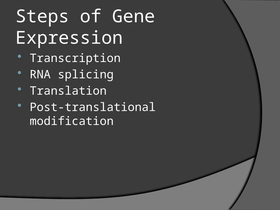
Steps of Gene Expression Transcription RNA splicing Translation Post-translational modification

What is Gene Expression Profiling? It is the measurement of the expression

of thousands of genes at once, to create a global picture of cellular function.

can distinguish between cells that are actively dividing, or show how the cells react to a particular treatment.

Gene Expression Profiling

Expression profiling is a logical next step after sequencing a genome: the sequence tells us what the cell could possibly do, while the expression profile tells us what it is actually doing now.

http://www.accessexcellence.org/RC/VL/GG/images/microarray_technology.gif

BIOINFORMATICS OF GENE EXPRESSION PROFILING.

http://www.wormbook.org/chapters/www_germlinegenomics/germlinegenomicsfig1.jpg

Normalization Filtering Data Statistical analysis Clustering Gene Ontology Pathway analysis

SNP Single nucleotide polymorphism also termed as

simple nucleotide polymorphism SNPs are single nucleotide variation observed

in the human genome. Eg… AAGCCTA to AAGCTTA, Presence of 2

allele. For a variation to be considered a SNP, it must

occur in at least 1% of the population. SNPs, which make up about 90% of all human genetic variation, occur every 100 to 300 bases along the 3-billion-base human genome.

SNP (Contd….) SNPs can occur in coding (gene) and

noncoding regions of the genome. Although more than 99% of human DNA

sequences are the same, variations in DNA sequence can have a major impact on how humans respond to disease; environmental factors such as bacteria, viruses, toxins, and chemicals; and drugs and other therapies. This makes SNPs valuable for biomedical research and for developing pharmaceutical products or medical diagnostics.

SNP (Contd….) SNPs are also evolutionarily stable. Scientists believe SNP maps will help them identify

the multiple genes associated with complex ailments such as cancer, diabetes, vascular disease, and some forms of mental illness.

SNPs do not cause disease, but they can help determine the likelihood that someone will develop a particular illness.

Eg…ApoE contains two SNPs that result in three possible alleles for this gene: E2, E3, and E4. Each allele differs by one DNA base, and the protein product of each gene differs by one amino acid.

FINAL WORDS

PRIVACY OF INDIVIDUALS IN A

COMPLEX DNA DATABASE

By

SundaresanRajasekaran

outline

Problem Definition Current status of the problem Methods and materials to asses the

problem Present current research going on Mathematical explanation of the present

work My views conclusion

Problems posed

Contributors are no longer anonymous. Can be tracked back very easily. Identify the potential medical issues of

the contributors. Data no longer available for the

researchers.

Background

All humans are 99.9% exactly the same. The 0.1% difference is called the ‘Single

Nucleotide polymorphism’ or SNP. Allele’s at a particular locus can be

classified as AA,AB or BB. To convert it mathematically the values

of allele’s can be considered as 0,0.5 and 1 corresponding to AA,AB and BB respectively.

How?

A mixture of various concentration was constructed.

Pick up any random individual – of any race (mostly from HapMap database).

Find the appropriate reference population by matching the mixture with the ancestral data.

Sample DataSNPs # Mixture Individual population

1234 0.5 1 0.5

1456 1 0.5 1

1567 0 1 1

1666 0 1 1

1667 0.5 0.5 0.5

1786 1 0.5 0.5

1799 0 0.5 0.5

1800 0 0 0

1999 0.5 1 0

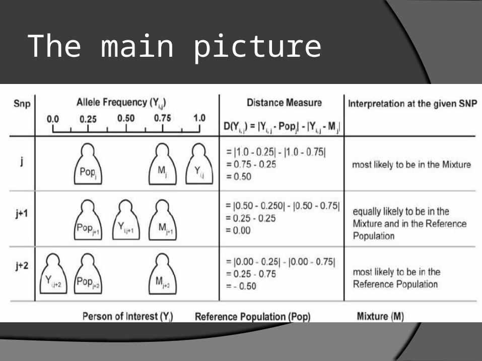
The main picture

Calculations We calculate D (Yi,j) = |Yi,j-Popj| - |Yi,j-Mj| Yi,j be the allele frequency estimate for the individual

i and SNP j We use the same formula’s to calculate Mj and

POPj. The first difference |Yi,j-Mj| measures how the allele

frequency of the mixture Mj at SNP j differs from the allele frequency of the individual Yi,j for SNP j.

The second difference |Yi,j-Popj| measures how the reference population’s allele frequency Popj differs from the allele frequency of the individual Yi,j for each SNP j.

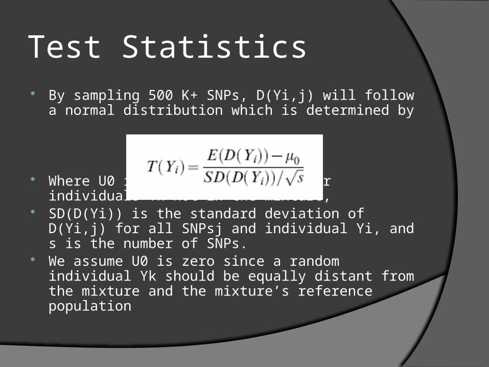
Test Statistics By sampling 500 K+ SNPs, D(Yi,j) will follow a

normal distribution which is determined by

Where U0 is the mean of D(Yk) over individuals Yk not in the mixture,

SD(D(Yi)) is the standard deviation of D(Yi,j) for all SNPsj and individual Yi, and s is the number of SNPs.

We assume U0 is zero since a random individual Yk should be equally distant from the mixture and the mixture’s reference population

The Normal Example:Testing

Test an hypothesis about the mean:

t-test

If , t follows a t-distribution with n-1 degrees of freedom

p-value

Experimental Validation

Can we improve?

Yes. How can we do that? By increasing the accuracy of the

existing system. i.e. Be able to reduce all the false positives.

Or, we can improve this method by reducing the number of SNPs. i.e. Do feature reduction.

What is feature reduction? Why feature reduction? Feature reduction algorithms Principal Component Analysis (PCA)

What is feature reduction? Feature reduction refers to the mapping of the

original high-dimensional data onto a lower-dimensional space.Criterion for feature reduction can be different

based on different problem settings.○ Unsupervised setting: minimize the information

loss○ Supervised setting: maximize the class

discrimination

High-dimensional data

Gene expression Face images Handwritten digits

What is feature reduction? Why feature reduction? Feature reduction algorithms Principal Component Analysis

Why feature reduction?

Most machine learning and data mining techniques may not be effective for high-dimensional data Query accuracy and efficiency degrade

rapidly as the dimension increases.

The intrinsic dimension may be small. For example, the number of genes

responsible for a certain type of disease may be small.

What is feature reduction? Why feature reduction? Feature reduction algorithms Principal Component Analysis

Feature reduction algorithms Unsupervised

Latent Semantic Indexing (LSI): truncated SVD

Independent Component Analysis (ICA)Principal Component Analysis (PCA)Canonical Correlation Analysis (CCA)

Supervised Linear Discriminant Analysis (LDA)

Application to microarrays

Dimension reduction (simplify a dataset)Clustering (two many samples)Discriminant analysis (find a group of

genes) Exploratory data analysis tool

Find the most important signal in data2D projections (clusters?)

Outline

What is feature reduction? Why feature reduction? Feature reduction algorithms Principal Component Analysis

What is Principal Component Analysis? Principal component analysis (PCA)

Reduce the dimensionality of a data set by finding a new set of variables, smaller than the original set of variables

Retains most of the sample's information.Useful for the compression and classification of data.

By information we mean the variation present in the sample, given by the correlations between the original variables. The new variables, called principal components

(PCs), are uncorrelated.

40

Principal Component Analysis (PCA)

• Information loss

− Dimensionality reduction implies information loss !!− PCA preserves as much information as possible:

• What is the “best” lower dimensional sub-space? The “best” low-dimensional space is centered at the sample mean

and has directions determined by the “best” eigenvectors of the

covariance matrix of the data x.

− By “best” eigenvectors we mean those corresponding to the largesteigenvalues ( i.e., “principal components”).

41

Principal Component Analysis (PCA)• Geometric interpretation

− PCA projects the data along the directions where the data varies the most.

− These directions are determined by the eigenvectors of the covariance matrix corresponding to the largest eigenvalues.

− The magnitude of the eigenvaluescorresponds to the variance of the data along the eigenvector directions.

Singular Value Decomposition (SVD)

• Given any mn matrix A, algorithm to find matrices U, V, and W such that

A = UWVT

U is mn and orthonormal

W is nn and diagonal

V is nn and orthonormal

SVD

T

1

00

00

00

VUA

nw

w

Quick Summary of PCA

1. Organize data as an m × n matrix, where m is the number of measurement types and n is the number of samples.

2. Subtract off the mean for each measurement type.3. Calculate the SVD or the eigenvectors of the covariance.

To Perform SVD, first calculate the new matrix Y such that

Y ≡ (1 /√n) XT

where Y is normalized along its dimensions.

Performing SVD on Y yields the Principal components of X.

Questions?

CLUSTERING ALGORITHMS FOR GENE EXPRESSION FILES

Bianca Lott

Teng Li

CS 144

Characteristics of Clustering Algorithms Hierarchial -algorithms that find successive

clusters using previously established clusters. Hirarchial algorithms can be

agglomerative(bottom-up) or divisive(top-down)

Agglomerative algorithms begin with each element as a separate cluster and merge them into larger clusters.

Divisive algorithms begin with the whole set and divide it into smaller clusters.

Characteristics of Clustering Algorithms(Cont’d) Partitional algorithms determine clusters all at

once. Density-based clustering algorithm is where a

cluster regarded as a region in which the density of data objects exceeds a threshold. DBSCAN and OPTICS are two typical algorithms of this kind.

Two-way clustering, co-clustering or biclustering are clustering methods where not only the objects are clustered but also the features of the objects, i.e., if the data is represented in a data matrix the rows and columns are clustered simultaneously.

Characteristics of Clustering Algorithms Many clustering algorithms require

specification of the number of clusters to produce the input data set, prior to execution of the algorithms.

Types of Clustering Algorithms that Optimize Some Quantities

CLIQUE[3]- fixes the minimum density of each dense unit by user parameter and searches for clusters that maximize the number of selected attributes.

PROCLUS[1]- requires a user parameter, l, to determine the number of attributes to be selected.

ORCLUS[2]- is close to the PROCLUS algorithm, except it adds a merging process of clusters and asks each cluster to select principal components instead of attributes.

Types of Clustering Algorithms that Optimize Some Quantities(Cont’d)

DOC and FastDOC algorithm-fix the maximum distance between attribute values by a user parameter.

In all these algorithms, the user parameter determines the attributes to be selected and the clusters to be formed.

If the wrong parameter is used, then the clustering accuracy is not diminished.

What You Want in a Projected Clustering Algorithm One with minimal input or use of parameters,

since the parameters are usually unknown. One with a deterministic characteristic or

follows one path to produce accurate results in a timely manner.

One with excellent recall values so that the selection of relevant attributes is accurate.

Relevance Index Local Variance Global Variance

Low local variance does not imply high relevance Relevance Index

A baseline to determine the relevance of an attribute to a cluster

Will Be Used in Two Parts of the AlgorithmAttribute Selection

○ Each cluster selects all attributes above a dynamic threshold

Similarity Calculation○ Hierarchical clustering merging order

Mutual Disagreement

Merge using RSim is guaranteed to be the highest quality Mutual Disagreement

Two merging clusters are not similar○ Big merges with small○ One with substantial attributes VS one with few

Relative relevance of attribute a to cluster C with the potential new cluster Cn

Severity of MD can be calculated by the following Use MD to reject heavy MD

HARP Algorithm• is a hierarchical approach with automatic relevant

attribute selection for projected clustering.• does not rely on user parameters in determining

relevant attributes in a cluster.• Tries to maximize the relevance index of each

selected attribute and the number of selected attributes of each cluster at the same time.

• Two thresholds(Amin, Rmin) are in place to restrict the minimum number of selected attributes for each cluster and the minimum relevance index values of them.

HARP Algorithm• // d: dataset dimensionality• // jAjmin: min. no. of selected attributes per cluster• // Rmin: min. relevance index of a selected attribute• Algorithm HARP(k: target no. of clusters)• Begin• 1 // Initially, each record is a cluster• 2 For step := 0 to d- 1 do {• 3 |A|min := d -step• 4 Rmin := 1 - step=(d-1)• 5 For each cluster C• 6 SelectAttrs(C,Rmin)• 7 BuildScoreHeaps(|A|min,Rmin)• 8 While global score heap is not empty {• 9 // Cb1 and Cb2 are the clusters involved in the• 10 // best merge, which forms the new cluster Cn• 11 Cn := Cb1 U Cb2• 12 SelectAttrs(Cn,Rmin)• 13 Update score heaps• 14 If clusters remained = k• 15 Goto 18• 16 }• 17 }• 18 Output result• End

Attribute Selection Procedure

Experiments Metrics

Synthetic Datasets

Real Datasets○ Datasets used in studying larger B-cell lymphoma

96 samples, 4026 expression values each. Expression values of the gene as attributes and has

been categorized into 9 classes

Metrics-Continued

Similarity FunctionsNon-projected algorithms

○ Euclidean Distance○ Pearson Correlation

Two hierarchic algorithms○ RSim

Performance MetricsAdjust Rand Index

○ 1 for 100% match and 0 for a random partition

Performance Results

Analyzing Real Data

Proclus and Harp are of the best performance For Proclus

Average is very low – 0.27

HARP Algorithm Analysis

Worst Case Time Complexity O(N*N*d*(d+logN)) --Loose Upper Bound No Repeated Runs

Summary – Comparisons of Projected Clustering Algorithms

The HARP algorithm was the best one out of all the algorithms (PROCLUS, ORCLUS, FastDoc).

The other algorithms only produced sufficient results when the correct parameters were used.

HARP produced accurate results in a single run.

HARP had excellent recall values so it could accurately select relevant attributes.

QUESTIONS?