Embed Size (px)
Citation preview
8
Saturn’s Ionosphere
L. MOORE1, M. GALAND
2, A.J. KLIORE
3, A.F. NAGY
4, AND J. O’DONOGHUE
5
1 Center for Space Physics, Boston University, Boston,
MA, USA. 2 Space and Atmospheric Physics Group, Department
of Physics, Imperial College London, London, UK. 3 Jet Propulsion Laboratory, California Institute of
Technology, Pasadena, CA, USA. 4 Department of Climate and Space Sciences and
Engineering, University of Michigan, Ann Arbor, MI,
USA. 5 NASA Goddard Space Flight Center, Greenbelt, MD,
USA.
Copyright Notice
"The Chapter, 'Saturn's Ionosphere: ring rain and other
drivers', is to be published by Cambridge University Press
as part of a multi-volume work edited by Kevin Baines,
Michael Flasar, Norbert Krupp, and Thomas Stallard,
entitled “Saturn in the 21st Century” (‘the Volume’)
© in the Chapter, L. Moore, M. Galand, A.F. Nagy, & J.
O’Donoghue © in the Volume, Cambridge University Press
NB: The copy of the Chapter, as displayed on this website,
is a draft, pre-publication copy only. The final, published
version of the Chapter will be available to purchase through
Cambridge University Press and other standard distribution
channels as part of the wider, edited Volume, once
published. This draft copy is made available for personal
use only and must not be sold or re-distributed."
Abstract
This chapter summarizes our current understanding of
the ionosphere of Saturn. We give an overview of
Saturn ionospheric science from the Voyager era to the
present, with a focus on the wealth of new data and
discoveries enabled by Cassini, including a massive
increase in the number of electron density altitude
profiles. We discuss recent ground-based detections
of the effect of “ring rain” on Saturn’s ionosphere, and
present possible model interpretations of the
observations. Finally, we outline current model-data
discrepancies and indicate how future observations can
help in advancing our understanding of the various
controlling physical and chemical processes.
8.1 Introduction
Saturn’s upper atmosphere is typically defined to be
the region above the homopause, which marks the
transition between a well-mixed atmospheric region
dominated by eddy diffusion below (the lower
atmosphere; Chapter 14) and a region dominated by
molecular diffusion above. It can further be broken
down into two coincident regions: the neutral
thermosphere (Chapter 9), and the charged ionosphere.
The upper atmosphere forms the transition region
between a dense neutral atmosphere below and a
tenuous, charged magnetosphere above (Chapter 6);
consequently it also mediates the exchange of
particles, momentum, and energy between these two
regions. External forcing on the upper atmosphere,
such as by solar extreme ultraviolet (EUV) photons or
energetic particles, determines the degree of ionization
within the ionosphere. As magnetic fields strongly
influence charged particle motions, the ionosphere
tends to be more strongly ionized where magnetic field
configurations favor precipitation of energetic particles
2 Moore, Galand, Kliore, Nagy & O’Donoghue
into the atmosphere; namely, the auroral regions near
the magnetic poles (Chapter 7).
In this chapter we summarize our current
understanding of the non-auroral ionosphere of Saturn,
drawing from ground-based and space-based
measurements (Section 8.2) and from modeling studies
for interpreting the observations and physical
processes driving Saturn’s ionosphere (Section 8.3).
As giant planet ionospheres are all qualitatively similar
we try to avoid reproducing material unnecessarily
from previous giant planet review articles. Therefore,
those reviews are still highly relevant (e.g., Atreya et
al., 1984; Waite et al., 1997; Nagy and Cravens, 2002;
Majeed et al., 2004; Yelle and Miller, 2004; Nagy et
al., 2009; Schunk and Nagy, 2009). While we will
touch upon closely related topics as appropriate, more
thorough discussions of Saturn’s aurorae and
thermosphere can be found in chapters 7 and 9,
respectively.
8.2 Observations
There are several options for remotely observing
Saturn’s ionosphere, and each technique has not only
particular advantages but also significant, unique
limitations. To date, the vast majority of observational
information regarding Saturn’s ionosphere has come
from spacecraft radio occultations, which yield vertical
electron density structure, Ne(h). Due to Sun-Saturn-
Earth geometry, however, a spacecraft-to-Earth radio
occultation can only be performed near the terminator
and therefore samples only the dawn or dusk
ionosphere of Saturn (see Section 8.2.1). An
additional method of tracking the peak ionospheric
electron density, NMAX, involves the detection of
broadband radio emission (dubbed Saturn Electrostatic
Discharge, SED) originating from powerful lightning
storms in Saturn’s lower atmosphere. As the storm
rotates, a nearby spacecraft can use SED emission to
derive the diurnal variation of NMAX near the storm
location. Unfortunately this technique is reliant upon
storm activity and latitude, and it does not contain any
altitude information (Section 8.2.2). Finally, infrared
measurements of rotational-vibrational emissions from
H3+ near 3-4 m yield temperature and density
information for this major ion in Saturn’s ionosphere.
Aside from one so-far-unique observation, however,
H3+ emission has proven to be too weak to be detected
outside of Saturn’s auroral regions (Section 8.2.3).
8.2.1 Radio Occultations
The technique of radio occultation, whereby Saturn’s
atmosphere occults the transmission of a radio signal
from a spacecraft to Earth (e.g., Lindal, 1992; Kliore et
al., 2004), provides the only available remote
diagnostic of electron density altitude profiles, Ne(h), a
basic ionospheric property. There are, at most, two
opportunities for deriving atmospheric properties
during a spacecraft flyby: one during the occultation
ingress (or entry, often designated with “N”) and one
during the occultation egress (or exit, often designated
with “X”). The geometry for essentially all of the
radio occultations performed at Saturn to date is such
that the ingress occultations sample the dusk
ionosphere while the egress occultations sample the
dawn ionosphere. Radio occultation latitude, typically
given in planetographic coordinates, refers to the
latitude at the lowest altitude of the occultation. As
the spacecraft almost never follows a trajectory in
which the occultation ray path is continually above a
single latitude, however, the altitude profile derived
from a radio occultation actually samples a range of
latitudes. Quoted radio occultation latitudes therefore
usually refer to either an approximate latitude or to the
latitude at the base of the occultation near the electron
density peak.
The main approach for analyzing spacecraft radio
occultations is based on geometrical optics (e.g.,
Fjeldbo et al., 1971). In this approach, the deviation
of a ray path in response to refractive index gradients
in ionospheric plasma is tracked, leading ultimately to
a Doppler shift in the frequency of the signal received
at Earth. The time series of differences between the
Saturn’s Ionosphere 3
transmitted and received frequencies, called the
frequency residuals, can then be used to derive a
vertical profile of refractive index and electron number
density (e.g., Withers et al., 2014). This direct
approach is particularly susceptible to multipath
propagation effects, wherein narrow ionospheric layers
can lead to multiple, distinct signals arriving
simultaneously at the receiving antenna, each with a
different Doppler-shifted frequency. This effect is
stronger the farther a spacecraft is away from the
occulting planet. A better approach is to first use
scalar diffraction theory, which transforms the data
using Fourier analysis in order to mimic an occultation
by a nearby spacecraft, thereby removing
complications due to multipath propagation and
diffraction effects (e.g., Karayel and Hinson, 1997;
Hinson et al., 1998). Once this is accomplished the
geometric approach can then be used. Saturn radio
occultations have so far only been analyzed by the
geometrical optics technique and therefore are highly
uncertain in the presence of narrow ionospheric layers,
which appear to be particularly common at lower
altitudes. In addition to instrumental effects, other
important sources of uncertainty include: the required
assumption of spherical symmetry within the
ionosphere, the degree of intervening plasma between
the transmitting and receiving antenna, and inaccurate
positions or velocities. The propagation of
uncertainties through all of the processing steps is non-
trivial (e.g., Lipa and Tyler, 1979), but typical
estimates are on the order of a few hundred electrons
per cubic centimeter for Cassini radio occultations
(Nagy et al., 2006; Kliore et al., 2011).
Flybys of the Saturn system by Pioneer 11 (1
September 1979), Voyager 1 (12 November 1980) and
Voyager 2 (26 August 1981) yielded our first
observational insights into Saturn’s ionospheric
electron densities (Kliore et al., 1980; Lindal et al.,
1985). While there was some variation in the electron
density profiles obtained by the Pioneer 11 and
Voyager spacecraft, the altitudes of the electron
density peaks (hMAX) ranged from ~1000-2800 km and
the maximum electron density (NMAX) of 5 out of the 6
profiles was of order 104 cm
-3. The Voyager 2 ingress
profile was an outlier from this trend, with narrow
low-altitude layers of peak electron density near
7x104 cm
-3. Such layers appear to be relatively
common in the giant planet ionospheres, as they have
also been found at Jupiter (e.g., Fjeldbo et al., 1975;
Yelle and Miller, 2004), Uranus (Lindal et al., 1987),
and Neptune (Lindal, 1992). While there is a lack of
consensus regarding the origin of these layers, a likely
explanation is that vertical wind shears – such as those
that might result from atmospheric gravity waves –
can lead to localized electron density enhancements.
This effect has been demonstrated through modeling
of Saturn’s upper atmosphere by Moses and Bass
(2000) and Barrow and Matcheva (2013), and also of
Jupiter (Matcheva and Strobel, 2001) and Neptune
(Lyons, 1995).
The arrival of Cassini at Saturn in 2004 has
significantly increased the number of radio
occultations, allowing for a more thorough
examination of possible ionospheric trends. A total of
59 Cassini radio occultations have already been
obtained and analyzed, with one final occultation
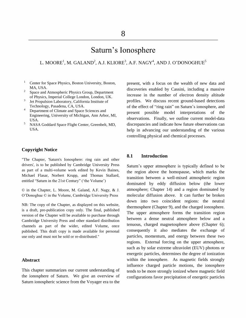
currently planned (Kliore et al., 2014). The first dozen
Cassini radio occultations were obtained between May
and September 2005 and sampled Saturn’s near-
equatorial region between 10oN and 10
oS
planetographic latitude. These profiles, shown in
Figure 8.1, revealed a clear dawn-dusk asymmetry.
While there is still a high degree of variability among
the 12 profiles, on average the peak densities are lower
and the peak altitudes are higher at dawn than at dusk
(Nagy et al., 2006). This trend is also present in the
complete Cassini radio occultation dataset, which
includes a number of additional low-latitude profiles
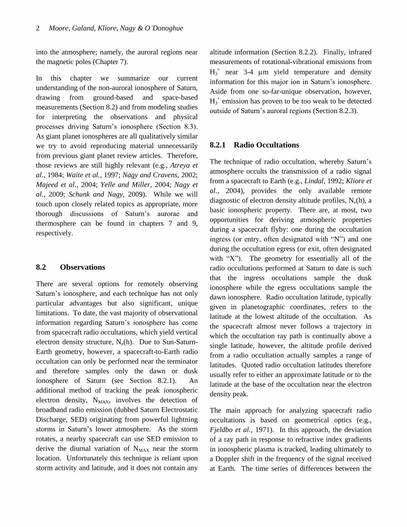
(Kliore et al., 2014). Such a behavior is consistent
with the expectation that chemical losses during the
Saturn night would lead to a depletion of the low-
altitude ionospheric electron density peak. The
averages of the first dozen low-latitude Cassini
profiles (5 dusk and 7 dawn) are shown in Figure 8.2.
4 Moore, Galand, Kliore, Nagy & O’Donoghue
Figure 8.1: Saturn ionospheric electron density altitude profiles retrieved from radio occultations by the Cassini
spacecraft at (left) dawn and (right) dusk. Also shown for comparison are Pioneer 11 and Voyager radio
occultation profiles. Error bars represent the uncertainties introduced by baseline frequency fluctuations and the
effects of averaging data from multiple Deep Space Network stations. All Cassini profiles are from ±10o latitude.
From Nagy et al. (2006).
Figure 8.2: Weighted averages of the dawn and
dusk electron density profiles from Figure 8.1.
From Nagy et al. (2006).
Subsequent Cassini radio occultations sampled a
wider range of latitudes, revealing a surprising trend
in NMAX. Nineteen low-, mid- and high-latitude radio
occultations obtained between September 2006 and
July 2008 found that peak electron densities were
smallest at Saturn’s equator, and increased with
latitude (Kliore et al., 2009). The average sub-solar
latitude during this occultation period was -8.5o,
meaning that the sun primarily illuminated Saturn’s
low latitudes. Solar EUV photons are expected to be
the primary source of ionization in Saturn’s non-
auroral ionosphere, and yet Cassini radio occultations
revealed the minimum electron densities to be in
regions of maximum insolation.
This latitudinal electron density trend was
reconfirmed and bolstered with 28 additional
occultations obtained between 2008 and 2013 (Kliore
et al., 2014). While there are a few high altitude
occultations, unfortunately none of them appear to
have sampled active auroral regions (Moore et al.,
2010).

Saturn’s Ionosphere 5
Figure 8.3: Total Electron Content (TEC) from all 59 published Cassini radio occultations. Dawn (exit) profiles are
shown as open circles, dusk (entry) profiles are shown as filled circles. Gray squares represent the local mean over
10o latitude bins. Vertical gray bars indicate the standard deviation of the mean, while horizontal gray bars
demarcate the latitude range over which the mean is calculated. Based on Table 1 of Kliore et al. (2014).
Figure 8.3 shows the total electron content (TEC), or
column integrated electron density, for all 59 of the
published Cassini radio occultations, plotted versus
planetographic latitude. The trend in TEC is quite
similar to that in NMAX, though with considerably less
scatter (Kliore et al., 2014). In both cases, there is a
clear minimum in electron density at Saturn’s
equator, and an increase in electron density with
latitude. There also appears to be a local minimum in
electron density around 45oN latitude, near the region
of Saturn’s atmosphere that is magnetically linked to
the inner B ring, long predicted to be the site of an
enhanced influx of water from the rings to the
atmosphere (e.g., Connerney and Waite, 1984;
Connerney, 1986). The introduction of oxygen,
whether in the form of neutral or charged water or
other oxygen-bearing molecules or charged sub-
micrometer grains, acts to reduce the local electron
density, as it converts the long-lived atomic ion H+
into a short-lived molecular ion. While it is tempting
to associate the localized minimum in electron
density near 45oN with an enhanced water influx,
ring-derived water influxes are expected to be
stronger in the southern hemisphere due to Saturn’s
effectively offset magnetic dipole (Burton et al.,
2010), independent of Saturn season (e.g., Northrop
and Connerney, 1987; Tseng et al., 2010). No similar
localized minimum is obvious in the southern
hemisphere radio occultations. There is a slight hint
of a minimum near 45oS, though the sampling
statistics are poor in that region.
Cassini radio occultation measurements have
demonstrated that Saturn’s ionosphere is highly
variable, with electron density altitude profiles
obtained at similar latitudes from similar times often
differing significantly from each other, and with
frequent narrow low-altitude layers of electron
density. Nevertheless, the wealth of data – at least
compared with other giant planet ionospheres – has
also allowed for identification of a number of trends.
On average, peak electron densities are smaller and
peak altitudes are higher at dawn than at dusk,
consistent with recombination of major ions during
the Saturn night. On average, the smallest electron
densities are found near Saturn’s equator, and

6 Moore, Galand, Kliore, Nagy & O’Donoghue
electron densities increase with latitude, contrary to
what would be expected from an ionosphere driven
purely by solar photoionization with constant
photochemical loss sources. Finally, though the
statistics are poor, radio occultation observations also
give some indication that there may be localized
minima in electron density near 45oN planetographic
latitude, which could be consistent with an influx of
charged water grains from Saturn’s rings to its
atmosphere along magnetic field lines.
8.2.2 Saturn Electrostatic Discharges (SEDs)
During Voyager encounters with Saturn, the
Planetary Radio Astronomy (PRA) instrument
detected mysterious, broadband, short-lived,
impulsive radio emission (Warwick et al., 1981,
1982). These radio bursts, termed Saturn
Electrostatic Discharges (SEDs), were organized in
episodes lasting several hours and separated from
each other by roughly 10h 10m. While there was
initially some uncertainty regarding the origin of
SEDs, Burns et al. (1983) suggested they were radio
manifestations of atmospheric lightning storms, and
Kaiser et al. (1984) demonstrated that an extended
source region in the equatorial atmosphere was
consistent with the observed SED recurrence pattern.
Cassini’s Radio and Plasma Wave Science (RPWS)
instrument began detecting SEDs prior to its orbital
insertion on 1 July 2004, and has since observed nine
distinct storm periods, separated by SED-quiet
periods of a few days to 21 months (Fischer et al.,
2011b). Shortly after Cassini’s arrival at Saturn, the
Imaging Science Subsystem instrument detected a
storm system at 35oS planetocentric latitude that
correlated with the observed SED recurrence pattern
(Porco et al., 2005). Dyudina et al. (2007) extended
this finding by presenting three further storm systems
where SED observations were correlated with the
rising and setting of a visible storm on the Saturn
radio horizon. Finally, lightning flashes were imaged
directly by Cassini in 2009, providing a convincing
demonstration that SEDs were indeed radio
signatures of atmospheric storms in Saturn’s lower
atmosphere (Dyudina et al., 2010).
SEDs have a large frequency bandwidth, but appear
as narrow banded streaks in both Voyager PRA and
Cassini RPWS dynamic spectra due to the short
duration of the radio burst and the frequency
sampling nature of the receivers. The number of
SEDs detected in an individual storm varies
significantly, from hundreds to tens of thousands
(Fischer et al., 2008), with typical burst rates of a few
hundred per hour (Zarka and Pedersen, 1983; Fischer
et al., 2006). SED storms are periods of nearly
continuous SED activity, modulated by episodes of
varying SED activity. The recurrence period of the
episodes within a storm represents the time between
peaks of SED activity; for a single longitudinally
confined storm system, therefore, this period is
closely related to the local rotation rate of the
atmosphere.
Recurrence periods for Voyager 1 and 2 SED
episodes were ~10h 10m and ~10h 00m, respectively
(Evans et al., 1981; Warwick et al., 1982), and were
consequently thought to originate from equatorial
storm systems (Burns et al., 1983), though none were
observed directly. In contrast, the majority of
recurrence periods for Cassini era SED storms are
near 10h 40m (Fischer et al., 2008), implying a mid-
latitude origin, as confirmed by the 35oS
planetocentric latitude storm clouds and visible
lightning flashes imaged by Cassini. Approximately
16 months after Saturn passed through its equinox
(August 2009) towards southern winter, a giant
convective storm developed at 35oN planetocentric
latitude, accompanied by unprecedented levels of
SED activity, with flash rates an order of magnitude
higher than previously observed storms (Fischer et
al., 2011a; this storm is described in detail in
Chapter 13). While the tendency for Saturn lightning
storms to preferentially form near ±35o planetocentric
latitude remains unexplained, it is important to keep
in mind that SEDs appear to primarily probe either
Saturn’s mid-latitude (Cassini era) or equatorial
(Voyager era) ionosphere.

Saturn’s Ionosphere 7
Figure 8.4: Diurnal variation in NMAX derived from Voyager 1 and Cassini SED observations (filled circles), along
with a least-squares fit to an equation of the form log Ne = A – B cos(SLT – ), where SLT is solar local time in
hours and is the phase shift (the dotted, dashed, and dot-dash curves). (a) Voyager 1, taken from Figure 4 of
Kaiser et al. (1984); (b) Voyager 1, taken from Figure 8 of Zarka (1985); and (c) Cassini, based on Figure 11 of
Fischer et al. (2011). The Voyager 1 fits (i.e., dotted and dashed curves) are repeated in (c) in order to more easily
compare them with the diurnal variation derived from Cassini era SEDs (dot-dash curve). Adapted from Figure 1 of
Moore et al. (2012).
SEDs originating from lightning storms deep within
Saturn’s atmosphere must ultimately transit the
ionosphere in order to be detected by a spacecraft.
Therefore, the low frequency cutoff of each SED
episode provides information about the intervening
plasma densities, as only frequencies larger than the
peak electron plasma frequency will pass through
Saturn’s ionosphere. Kaiser et al. (1984) combined
the observed low frequency cutoffs with a ray tracing
analysis in order to derive the peak electron density
along the propagation path between Voyager 1 and
the SED storm. Using similar assumptions, Zarka
(1985) also derived peak electron densities from
Voyager 1 SED measurements. (Voyager 2 data
showed a decline in number and intensity of SEDs
with no clear episodic behavior, meaning it could not
be used for a similar analysis.) Both Kaiser et al.
(1984) and Zarka (1985) found that NMAX varied by
more than two orders of magnitude throughout the
Saturn day, with midnight electron densities below
103 cm
-3 and noon densities greater than 10
5 cm
-3.
The SED-derived dawn and dusk NMAX values were
of order 104 cm
-3, in rough agreement with radio
occultation results. These diurnal NMAX trends, along
with a Cassini era SED-derived trend, are presented
in Figure 8.4.
Whereas Voyager 1 NMAX trends were derived from
three SED episodes, Cassini SED observations
allowed for investigation of diurnal trends over
different storm periods, different episodes within
storm periods, and different Cassini-Saturn distances.
The diurnal NMAX trend shown in Figure 8.4c was
based on 48 SED episodes between 2004 and 2009
when Cassini was within 14 RS of Saturn (Figure 11
of Fischer et al., 2011b). This profile is slightly
different from the Cassini era trend that includes all
of the SED observations through 2009 (Figure 9 of
Fischer et al., 2011b), most likely due to the fact that
attenuation of radio waves by Saturn’s ionosphere is
frequency-dependent, and Cassini is better able to
detect weaker bursts at lower frequencies when it is
nearer to Saturn. In contrast to the two-order-of-
magnitude diurnal variation in NMAX derived from
Voyager SEDs, the Cassini SED-derived NMAX varies

8 Moore, Galand, Kliore, Nagy & O’Donoghue
by only one order of magnitude, between ~104 cm
-3
and ~105 cm
-3, with a local minimum just before
sunrise. Such a local minimum in electron density is
consistent with the nighttime chemical loss due to
recombination implied by radio occultations; a
minimum at midnight is much more difficult to
understand theoretically (e.g., Majeed and
McConnell, 1996).
While peak electron densities derived from SEDs are
highly complementary to the dawn/dusk electron
density profiles retrieved from radio occultation
measurements, there are also some unique limitations
to bear in mind. First, the frequency-dependent
attenuation of radio waves by Saturn’s ionosphere
highlights an ambiguity regarding the observed cutoff
frequency. For example, Fischer et al. (2011b) find a
correlation between Cassini-Saturn distance and
cutoff frequency: on average Cassini observes lower
cutoff frequencies (and therefore derives lower NMAX
values) when it is closer to Saturn. There are
relatively few SED episodes with Cassini closer than
5 RS, however, so it is not clear whether this trend
continues radially inwards towards Saturn. If so, it
may imply that the current derived NMAX values
should be reduced in magnitude. It is not
immediately obvious how such a correlation would
affect the Voyager era results, though it is worth
noting that the anomalously low frequency cutoffs
occurred during Voyager’s closest approach (Kaiser
et al., 1984). These anomalous low frequency cutoffs
also occurred near ~300-600 kHz, where Saturn
kilometric radiation, or SKR, typically dominates the
frequency spectrum, a fact that can complicate SED
analysis (Fischer et al., 2011b).
The second main limitation of SED observations is
the uncertainty regarding the portion of the
ionosphere sampled by the transiting radio waves.
Over-horizon SEDs have been observed regularly by
Cassini – that is, SED detections prior to the rising of
their originating storm above the horizon as seen by
the spacecraft (Fischer et al., 2008). These SEDs are
likely a result of ducting (Zarka et al., 2006), wherein
propagating radio waves are refracted by the
ionosphere, and their detection emphasizes that one
cannot rely on the assumption that SEDs traverse a
straight line from their origin to the observer.
Consequently it is possible that SEDs sample portions
of the ionosphere different from where the radio
signals originate. For example, shadowing by
Saturn’s rings leads to patterns of depleted electron
density that depend on season, and may help explain
the anomalously low frequency cutoffs observed by
Voyager (Burns et al., 1983; Mendillo et al., 2005).
Nevertheless, despite the above limitations, SEDs
provide valuable insight to Saturn’s ionosphere as
well as an additional observational constraint that
remains to be explained: the strong diurnal variation
of NMAX (of 1-2 orders of magnitude). While weak
SED-like radio spikes were detected by Voyager 2
during its encounters with Uranus (Zarka and
Pedersen, 1986) and Neptune (Kaiser et al., 1991),
no high-frequency radio emission from lightning was
detected at Jupiter by any visiting spacecraft, despite
whistler and optical lightning detections (Zarka et al.,
2008), possibly due to ionospheric attenuation
(Zarka, 1985b) or to slow lightning discharge
(Farrell et al., 1999).
8.2.3 Observations of ionospheric H3+
Since its initial discovery in the Jovian atmosphere
(Drossart et al., 1989), H3+ has been an effective
probe of the auroral ionospheres of Jupiter (e.g.,
Lystrup et al., 2008; Stallard et al., 2012b, and
references therein), Saturn (e.g., Stallard et al., 2008,
2012a; O’Donoghue et al., 2014, and references
therein; see also Chapter 7), and Uranus (Melin et al.,
2013). There is an abundance of strong H3+
rotational-vibrational emission lines available in the
near-IR, as described in Chapter 7. Ionization of
molecular hydrogen, the dominant constituent of
Saturn’s upper atmosphere, leads directly to the
production of H3+ via the rapid ion-molecule reaction
(H2+ + H2 H3
+ + H). Therefore H3
+, along with H
+,
is expected to be a major ion in giant planet
ionospheres. As H3+ is in quasi-local thermodynamic
Saturn’s Ionosphere 9
equilibrium with the neutral atmosphere in the
collisional region of the ionosphere, it also serves as a
valuable probe of upper atmospheric temperatures
(e.g., Miller et al., 2000).
At Jupiter, where ionospheric densities and upper
atmospheric temperatures are relatively large, H3+ can
be observed at all latitudes. Low- and mid-latitude
H3+ column densities at Jupiter are approximately
~3-5x10¹¹
cm-2
, whereas auroral column densities can
be more than 1012
cm-2
(Lam et al., 1997; Miller et
al., 1997). Auroral column densities at Saturn have
been measured to be of the same order, though
variable, with reported values between
~1-7x10¹²
cm-2
(Melin et al., 2007). The strong
dependence of H3+ emission on temperature,
however, has inhibited searches for non-auroral H3+ at
Saturn, due to the low equatorial temperatures
described in Chapter 9. Prior to 2011 the lowest
latitude of detected H3+ at Saturn was ~57
o
(planetographic south), a weak secondary auroral
oval thought to be associated with the breakdown in
corotation within the magnetosphere (Stallard et al.,
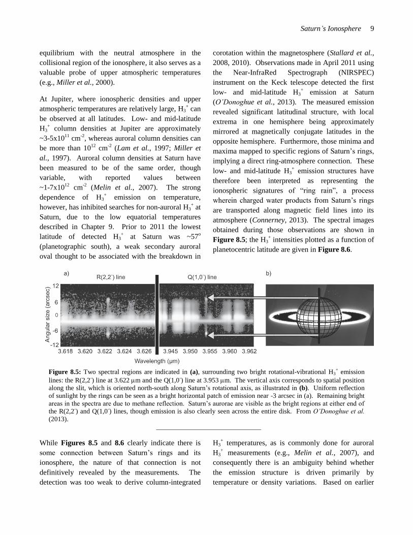
2008, 2010). Observations made in April 2011 using
the Near-InfraRed Spectrograph (NIRSPEC)
instrument on the Keck telescope detected the first
low- and mid-latitude H3+ emission at Saturn
(O’Donoghue et al., 2013). The measured emission
revealed significant latitudinal structure, with local
extrema in one hemisphere being approximately
mirrored at magnetically conjugate latitudes in the
opposite hemisphere. Furthermore, those minima and
maxima mapped to specific regions of Saturn’s rings,
implying a direct ring-atmosphere connection. These
low- and mid-latitude H3+ emission structures have
therefore been interpreted as representing the
ionospheric signatures of “ring rain”, a process
wherein charged water products from Saturn’s rings
are transported along magnetic field lines into its
atmosphere (Connerney, 2013). The spectral images
obtained during those observations are shown in
Figure 8.5; the H3+ intensities plotted as a function of
planetocentric latitude are given in Figure 8.6.
Figure 8.5: Two spectral regions are indicated in (a), surrounding two bright rotational-vibrational H3+ emission
lines: the R(2,2-) line at 3.622 m and the Q(1,0
-) line at 3.953 m. The vertical axis corresponds to spatial position
along the slit, which is oriented north-south along Saturn’s rotational axis, as illustrated in (b). Uniform reflection
of sunlight by the rings can be seen as a bright horizontal patch of emission near -3 arcsec in (a). Remaining bright
areas in the spectra are due to methane reflection. Saturn’s aurorae are visible as the bright regions at either end of
the R(2,2-) and Q(1,0
-) lines, though emission is also clearly seen across the entire disk. From O’Donoghue et al.
(2013).
While Figures 8.5 and 8.6 clearly indicate there is
some connection between Saturn’s rings and its
ionosphere, the nature of that connection is not
definitively revealed by the measurements. The
detection was too weak to derive column-integrated
H3+ temperatures, as is commonly done for auroral
H3+ measurements (e.g., Melin et al., 2007), and
consequently there is an ambiguity behind whether
the emission structure is driven primarily by
temperature or density variations. Based on earlier
10 Moore, Galand, Kliore, Nagy & O’Donoghue
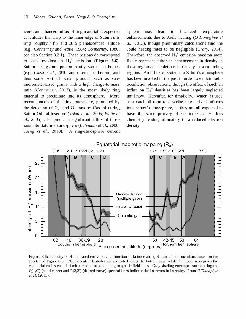
work, an enhanced influx of ring material is expected
at latitudes that map to the inner edge of Saturn’s B
ring, roughly 44oN and 38
oS planetocentric latitude
(e.g., Connerney and Waite, 1984; Connerney, 1986;
see also Section 8.2.1). These regions do correspond
to local maxima in H3+ emission (Figure 8.6).
Saturn’s rings are predominantly water ice bodies
(e.g., Cuzzi et al., 2010, and references therein), and
thus some sort of water product, such as sub-
micrometer-sized grains with a high charge-to-mass
ratio (Connerney, 2013), is the most likely ring
material to precipitate into its atmosphere. More
recent models of the ring ionosphere, prompted by
the detection of O2+ and O
+ ions by Cassini during
Saturn Orbital Insertion (Tokar et al., 2005; Waite et
al., 2005), also predict a significant influx of those
ions into Saturn’s atmosphere (Luhmann et al., 2006;
Tseng et al., 2010). A ring-atmosphere current
system may lead to localized temperature
enhancements due to Joule heating (O’Donoghue et
al., 2013), though preliminary calculations find the
Joule heating rates to be negligible (Crary, 2014).
Therefore, the observed H3+ emission maxima more
likely represent either an enhancement in density in
those regions or depletions in density in surrounding
regions. An influx of water into Saturn’s atmosphere
has been invoked in the past in order to explain radio
occultation observations, though the effect of such an
influx on H3+ densities has been largely neglected
until now. Hereafter, for simplicity, “water” is used
as a catch-all term to describe ring-derived influxes
into Saturn’s atmosphere, as they are all expected to
have the same primary effect: increased H+ loss
chemistry leading ultimately to a reduced electron
density.
Figure 8.6: Intensity of H3+ infrared emission as a function of latitude along Saturn’s noon meridian, based on the
spectra of Figure 8.5. Planetocentric latitudes are indicated along the bottom axis, while the upper axis gives the
equatorial radius each latitude element maps to along magnetic field lines. Gray shading envelopes surrounding the
Q(1,0-) (solid curve) and R(2,2
-) (dashed curve) spectral lines indicate the 1 errors in intensity. From O’Donoghue
et al. (2013).
Saturn’s Ionosphere 11
8.3 Models
We have outlined the available observational
constraints for Saturn’s ionospheric parameters in
Section 8.2. We now give an overview of the basic
theory used to explain these measurements, and
review the past modeling studies (Section 8.3.1). A
more thorough description of past ionospheric
modeling studies can be found in Nagy et al. (2009),
and so we touch only briefly on that history here.
Contemporary model-data comparisons are
highlighted in order to give context to the current
state of knowledge and to emphasize outstanding
model-data discrepancies (Section 8.3.2).
8.3.1 Basic Theory: Chemistry, Ionization,
and Temperature
Molecular hydrogen is the dominant constituent in
Saturn’s upper atmosphere, with atomic hydrogen
becoming important at the higher altitudes. At non-
auroral latitudes, the primary source of ionization is
solar X-ray (0.1-10 nm) and EUV (10-110 nm)
photons. As the dominant constituent, H2 absorbs
most of the incident radiation at those wavelengths,
and so the vast majority of photo-produced ions are
H2+. Maximum photoionization rates (i.e., overhead
illumination for solar maximum photon fluxes) for
H2+ and H
+ in Saturn’s ionosphere are roughly
10 cm-3
s-1
and 1 cm-3
s-1
, respectively (Moore et al.,
2004). Direct photoionization of methane also leads
to an array of hydrocarbon ions; CH4+ is produced
most rapidly, with a 2-3 cm-3
s-1
production rate,
though these ions are produced much lower in the
ionosphere, near the homopause, where their parent
species are located (Kim et al., 2014). While H2+ is
the dominant species created by photoionization, it is
quickly converted to H3+ via the charge-exchange
reaction (Theard and Huntress, 1974; see also Miller
et al., 2006, and references therein):
H2+ + H2 H3
+ + H (8.1)
Saturn’s ionosphere is thus predicted to be dominated
by a mix of H3+ and H
+ ions near the electron density
peak and above, with an additional ledge of
hydrocarbon ions below the peak, closer to the
homopause (e.g., Majeed and McConnell, 1991;
Moses and Bass, 2000; Moore et al., 2004; Kim et al.,
2014). The lower ionosphere (e.g., ~2300 km and
below for mid-latitudes) is expected to be in
photochemical equilibrium; for such conditions the
H+/H3
+ number density ratio is found to be
proportional to electron density (Moore et al., 2004).
Dissociative recombination between H3+ and
electrons – the dominant loss for H3+ ions – is rapid
relative to the Saturn day. Typical H3+ lifetimes are
~10-15 minutes in Saturn’s ionosphere (Melin et al.,
2011; Tao et al., 2011), much shorter than Saturn’s
~10 hour rotation period (see Chapter 5).
Consequently, for conditions of reduced electron
density, the H+/H3
+ ratio decreases, and the expected
diurnal variation of the electron density in the main
ionosphere increases (i.e., a smaller H+/H3
+ ratio
means a larger fraction of short-lived H3+ ions).
Early models of Saturn’s ionosphere (e.g., McElroy,
1973; Capone et al., 1977) predicted a peak electron
density an order of magnitude larger than subsequent
Pioneer and Voyager radio occultation measurements
revealed (Kliore et al., 1980; Lindal et al., 1985).
The only chemical loss included for H+ in these early
models was radiative recombination, an extremely
slow process. Therefore, in order to reduce modeled
electron densities to better reproduce the observed
values, a method of converting H+ to a short-lived ion
was required. The two methods considered by most
subsequent models are charge exchange between H+
and vibrationally excited H2, and charge exchange
with water introduced into the atmosphere from
Saturn’s rings and/or icy moons.
Vibrationally Excited H2
As was recognized early on (McElroy, 1973), the
charge-exchange reaction
12 Moore, Galand, Kliore, Nagy & O’Donoghue
H+ + H2(≥4) H2
+ + H (8.2)
is exothermic only when H2 is in the 4th or higher
vibrational level. While there has historically been
some uncertainty regarding the R8.2 reaction rate, it
has generally been assumed to be of the order
1-2x10⁻⁹
cm3 s
-1 (e.g. McConnell et al., 1982;
Cravens, 1987). Recent extrapolation of work by the
plasma fusion quantum theory community (e.g.,
Ichihara et al., 2000; Krstić, 2002) has been used to
refine the estimated R8.2 reaction rate (at 600 K) only
slightly, to 0.6-1.3x10⁻⁹
cm3 s
-1 (Huestis, 2008). Of
far greater uncertainty is the population of non-LTE
vibrationally excited H2, where LTE refers to local
thermodynamic equilibrium. (If the H2 vibrational
distribution were in LTE at 1000 K, fewer than 10-10
molecules would be in the ≥4 state, far too low a
value to significantly impact H+ densities.)
Molecular hydrogen in giant planet upper
atmospheres can be vibrationally excited by electron
impact, by solar and electron excitation of the H2
Lyman and Werner bands, which then fluoresce to
vibrationally excited levels in the ground state, and
by dissociative recombination of H3+ (e.g., Waite et
al., 1983; Cravens, 1987; Majeed et al., 1991).
Major vibrational loss processes include de-excitation
through collisions with H and H2, reactions with H+
(i.e., R8.2), and redistribution of vibrational quanta
among molecular levels through vibrational-
vibrational (V-V) collisions and in altitude through
diffusion.
The first detailed model for H2() in the outer planets
was presented by Cravens (1987) for Jupiter. Majeed
et al. (1991) added solar fluorescence in their low-
latitude solar input H2() calculations for Jupiter and
Saturn, finding it to be a dominant source of
vibrational excitation. Both Cravens (1987) and
Majeed et al. (1991) found modest enhancements in
H2(≥4) populations, leading to reductions in
calculated electron densities that were insufficient to
reproduce the observed electron density profiles. In
general, calculations of H2(≥4) appear to fall short
of the enhanced vibrational populations required to
bring modeled and observed electron densities into
agreement, possibly due to uncertainties in the
calculations (such as rate coefficients or source
mechanisms; Majeed et al., 1991), or possibly due to
other processes acting to reduce H+ densities. More
recently, Hallett et al. (2005a) developed a new
rotational-level hydrogen physical chemistry model,
and subsequently applied it to Uranus (Hallett et al.,
2005b).
Subsequent model reproductions of electron density
profiles from radio occultation observations have
typically modified H2(≥4) populations freely or have
used scaled versions of the Majeed et al. (1991)
calculations (e.g., Majeed and McConnell, 1996;
Moses and Bass, 2000; Moore et al., 2006). In other
words, partly due to uncertainties in direct H2(≥4)
calculations, and partly due to attention being focused
on other details of the Saturn ionosphere,
contemporary models have predominantly treated the
population of vibrationally excited H2 as a free
parameter. Reaction R8.2 directly reduces H+ ion
densities by converting H+ to short-lived molecular
ions, thereby indirectly reducing the net electron
density and reducing the dominant chemical loss for
H3+ – dissociative recombination with electrons. Due
to the long lifetime of H+, R8.2 can also act as an
additional source of H2+ (and H3
+ via R8.1), even in
regions absent of ionizing radiation or precipitating
energetic particles. Therefore, as it affects all of the
major chemistry, R8.2 and the true population of
vibrationally excited H2 remain major points of
uncertainty for ionospheric calculations. There are no
direct observational constraints published at present.
Water in Saturn’s Ionosphere
A second likely method of converting H+ ions into
short-lived molecular ions, thereby depleting the
calculated electron densities, begins with an influx of
water into Saturn’s atmosphere. Possible external
water sources include micrometeorites as well as
Saturn’s rings and icy satellites. This ionospheric

Saturn’s Ionosphere 13
quenching chain was first postulated by Shimizu
(1980), implemented by Chen (1983), and treated
comprehensively by Connerney and Waite (1984).
H+ + H2O H2O
+ + H (8.3)
H2O+ + H2 H3O
+ + H (8.4)
H3O+ + e
H2O + H
H2 + OH
H + H + OH
(8.5a)
(8.5b)
(8.5c)
As noted by Connerney and Waite (1984), any OH in
the system (such as that from R8.5) has a short
lifetime due to its reaction with H2, producing H2O
and H. Similarly, any ionized water products, such as
O2+, dissociatively recombine with electrons
extremely rapidly – roughly three times faster than
H3+ in Saturn’s ionosphere – leading to a chain of
photochemical reactions that produce primarily OH
(via O + H2) and H2O (via OH + H2) in the
thermosphere and lower atmosphere (e.g. Moses and
Bass, 2000; Moses et al., 2000). Hence, while the
exact form of exogenous influx may not always be
pure H2O, the ionospheric chemical effects are
similar.
The various reaction rates for water chemistry in
outer planet upper atmospheres are relatively well
known (e.g., Moses and Bass, 2000; Moses et al.,
2000). Of far greater uncertainty is the magnitude of
water influx at Saturn, as well as its spatial and
temporal distribution and variability. While a number
of modeling studies have derived a range of water
influxes indirectly as a means of reproducing the
electron density profiles from radio occultations (e.g.,
Connerney and Waite, 1984; Majeed and McConnell,
1991, 1996; Moore et al., 2006, 2010), directly
constraining the influxes observationally has proven
more difficult. The first unambiguous detection of
water in Saturn’s upper atmosphere came from the
Infrared Space Observatory (ISO; Feuchtgruber et
al., 1997), which measured an H2O column
abundance of (0.8-1.7)x1015
cm-2
and was used to
derive a global water influx of ~1.5x10⁶ H2O
molecules cm-2
s-1
(Moses et al., 2000). Subsequent
studies based on Submillimeter Wave Astronomy
Satellite and Herschel Space Observatory
measurements found global influx values within a
factor of 4 of the Moses et al. result (Bergin et al.,
2000; Hartogh et al., 2011). Despite predictions of
strong latitudinal variations in water influx (e.g.,
Connerney, 1986), no observational confirmation of
such variations has yet been published. At present,
there are ambiguous detections of latitudinally
varying water volume mixing ratios in the ultraviolet
(e.g., a 2 detection of 2.70x10¹⁶
cm-2
at 33oS
planetocentric latitude: Prangé et al., 2006) as well as
preliminary indications of larger equatorial water
densities from Cassini Composite InfraRed
Spectrometer (CIRS) observations (Bjoraker et al.,
2010) and from further Herschel observations
(Cavalié et al., 2014).
A number of different categories of theoretical
studies support the preliminary observational results
that favor a latitudinal variation of water influx at
Saturn. The first category includes ring modeling
studies focused on the erosion of Saturn’s rings (e.g.,
Northrop and Hill, 1982, 1983; Ip, 1983; Northrop
and Connerney, 1987). One of the outcomes of such
studies is the demonstration that small negatively
charged ring grains inside of a marginal stability
radius of 1.525 RS can be lost to Saturn’s atmosphere
along magnetic field lines. A recent related study
also explores the evolution of positively charged ring
grains, and finds that they are sometimes deposited in
Saturn’s equatorial atmosphere (Liu and Ip, 2014). A
second category of studies is focused on the ring
atmosphere and ionosphere, and likewise predicts a
precipitation of ring ions into Saturn’s atmosphere
(e.g., Luhmann et al., 2006; Tseng et al., 2010). In
general, all of the ring models predict an asymmetry
in the particle influx due to Saturn’s slightly offset
magnetic dipole, with stronger influxes expected in
the southern hemisphere. Finally, a third main
category of modeling studies that predict a latitudinal
variation of water influx at Saturn are those that track
the water vapor ejected from Enceladus’ plumes
(Porco et al., 2006). These models estimate that
approximately 10%, 7%, 3%, and 6%, respectively,

14 Moore, Galand, Kliore, Nagy & O’Donoghue
of the Enceladus water is lost to Saturn’s atmosphere
(Jurac and Richardson, 2007; Cassidy and Johnson,
2010; Hartogh et al., 2011; Fleshman et al., 2012).
Latitude variations of Saturn water influx from the
Enceladus models vary, though in general a stronger
influx is predicted at low-latitudes. Finally, temporal
(and possibly seasonal) variability is also expected
for both ring and Enceladus sources of water, though
it is not well constrained at present.
Primary and Secondary Ionization
Ionizing radiation at the giant planets comes
primarily in two forms: solar photons and energetic
particles. Electrons released during ionization are
usually suprathermal. These suprathermal electrons –
referred to as photoelectrons in the case of
photoionization and secondary electrons in the case
of particle impact ionization – possess enough energy
to excite, dissociate, and further ionize the neutral
atmosphere as well as to heat the plasma. On the one
hand, photoionization production rates follow from a
fairly straightforward application of the Lambert-
Beer Law, at least assuming that the neutral
atmospheric densities, incident solar fluxes, and
photoabsorption and photoionization cross sections
are known. Conversely, in order to accurately track
the transport, energy degradation, and angular
redistribution of suprathermal electrons, a kinetic
approach needs to be applied, such as solution to the
Boltzmann equation through a multi-stream approach
(Perry et al., 1999; Moore et al., 2008; Galand et al.,
2009; Gustin et al., 2009) or a Monte Carlo approach
(e.g., Tao et al., 2011). While ionization due to
photoelectrons and secondary electrons is usually
included in the case of Venus, Earth, Mars, Jupiter,
and Titan (e.g., Kim et al., 1989; Kim and Fox, 1994;
Schlesier and Buonsanto, 1999; Cravens et al., 2004;
Fox, 2004, 2007; Fox and Yeager, 2006; Galand et
al., 2006; Matta et al., 2014), it is this added
complexity that has prevented secondary ionization
from being treated in the majority of Saturn
ionospheric models.
Higher energy photons produce higher energy
photoelectrons, and therefore lead to more secondary
ionization. In general photoabsorption cross sections
are smallest for high energy photons and increase
nearly monotonically over their ionization range.
There are certainly exceptions to this generality (e.g.,
methane near 4 nm), however it holds true for H2 for
photons >1 nm – the dominant absorber in the outer
planets – meaning that more energetic photons are
typically absorbed lower in the atmosphere at Saturn
(Moses and Bass, 2000; Galand et al., 2009).
Secondary ionization due to solar illumination,
therefore, primarily increases the ion production rate
in the lower ionosphere.
In the auroral regions, precipitating particles interact
with the ambient atmosphere via collisions, leading to
excitation, ionization and heating. About half of all
inelastic collisions between precipitating energetic
electrons and Saturn’s upper atmosphere result in the
ionization of H2 that is initially in the electronic
ground state (X1g
+), producing both H2
+ and
secondary electrons es:
e + H2 H2+ + es + e (8.6)
Since this process does not remove the energetic
electrons, the precipitating electrons and their
secondary products undergo further inelastic
collisions, producing additional ionization, excitation,
and dissociation in the atmosphere, as well as heating
of thermal, ionospheric electrons. These energetic
particles lose kinetic energy with each collision until
they are finally thermalized with the surrounding
atmosphere. Atmospheric effects due to precipitating
energetic electrons (e.g., Galand et al., 2011; Tao et
al., 2011), such as ionization and heating, are
discussed in more detail in Chapters 7 and 9.
There are two studies that treat secondary ionization
comprehensively in Saturn’s non-auroral ionosphere.
The first, Galand et al. (2009), solves the Boltzmann
equation for suprathermal electrons using a
multistream transport model based on the solution
proposed by Lummerzheim et al. (1989) for terrestrial

Saturn’s Ionosphere 15
applications. A simple parameterization of secondary
ionization rates based on the Galand et al. (2009)
results appears in Moore et al. (2009), accurate over a
range of solar/seasonal conditions and latitudes. A
number of related modeling studies include either the
Galand et al. (2009) results or the Moore et al. (2009)
parameterization (e.g., Moore et al., 2010; Barrow
and Matcheva, 2013). The second study to calculate
secondary ionization rates at Saturn directly, Kim et
al. (2014), assumes that photoelectrons deposit their
energy locally using a simple method described by
Dalgarno and Lejeune (1971). A similar approach
has been used for Jupiter (e.g., Kim and Fox, 1994).
Both the Galand et al. (2009) and the Kim et al.
(2014) studies are for mid-latitude, and both find that
the secondary ionization production rates are roughly
comparable to primary photoionization rates just
below 1000 km altitude (i.e., for pressures greater
than ~10-5
mbar). At lower altitudes (higher
pressures) secondary ionization production rates are
dominant by as much as an order of magnitude. The
effect on calculated ion and electron densities is also
altitude-dependent: electron densities are increased
by roughly 30% at the peak and by up to an order of
magnitude at lower altitudes (Galand et al., 2009).
The impact of secondary ionization on Saturn
ionospheric electron densities is illustrated in
Figure 8.7, which shows the ratio of calculated
electron densities between simulations that do and do
not include the extra production term. It is clear from
Figure 8.7 that models of Saturn’s ionosphere that do
not account for secondary ionization in some form
will significantly underestimate electron densities in
Saturn’s lower ionosphere.
Figure 8.7: Contour plot of the electron density ratio between a simulation that includes secondary ionization (NeSI
)
and a run that ignores secondary ionization (Ne). Both simulations are for solar minimum conditions at mid-latitude.
From Galand et al. (2009).
Hydrocarbon ions
Most of the preceding discussion has focused on H+
and H3+, as those are the ions predicted to be
dominant throughout most of Saturn’s ionosphere.
There is, however, an additional predicted ledge of
low-altitude ionization, thought to be dominated by
hydrocarbon (and possibly metallic) ions, just above
the homopause. Many models treat the hydrocarbon
layer as an ionospheric sink, if they consider it at all,
as methane readily charge-exchanges with H+ and
H3+, leading to a relatively short-lived molecular
hydrocarbon ions (e.g., Moore et al., 2008, and
related studies). Such a treatment can lead to fairly
accurate electron densities within the hydrocarbon
layer, at least when compared with more
16 Moore, Galand, Kliore, Nagy & O’Donoghue
comprehensive models, but the resulting hydrocarbon
ion composition is incorrect (e.g., Moses and Bass,
2000; Moore et al., 2008).
There are two main complications that models must
address in order to treat hydrocarbon ions
comprehensively. First, there are numerous
hydrocarbon ions and a significantly more complex
series of reactions to consider. Depending on the
modeling approach, this may only hinder results by
requiring a larger table of ions and reactions to be
inserted, though even in that case many of the
reaction rates are unknown or untested in the
laboratory. The two models that treat the
hydrocarbon layer at Saturn most comprehensively
are Moses and Bass (2000) and Kim et al. (2014).
Moses and Bass consider 109 different ion species
with 845 reactions, while Kim et al. track 53 ions
using 749 reactions. Note that models developed for
Titan’s rich high-molecular-weight hydrocarbon
atmosphere include an even more complete list of
reactions and ions (e.g.,Waite et al., 2010; Vuitton et
al., 2015). The second complication that needs to be
addressed for accurate calculations of hydrocarbon
ion densities is that high resolution H2
photoabsorption cross sections (of the order of
10-4
nm) are required between ~80 nm (the H2
ionization threshold) and 111.6 nm. Photons across
this wavelength range, in which H2 absorbs in
discrete transitions – mostly in the Lyman, the
Werner, and the Rydberg band systems – possess
enough energy to ionize atomic hydrogen as well as
methane, and H2 photoabsorption cross sections can
differ by six orders of magnitude over very short
wavelength scales. Calculations that use low
resolution cross sections will absorb these photons
higher in the atmosphere, on average, before they can
ionize methane and other hydrocarbon neutrals near
the homopause; such models consequently under
predict photoionization rates within the hydrocarbon
layer. The only study so far to include high
resolution H2 photoabsorption cross sections at Saturn
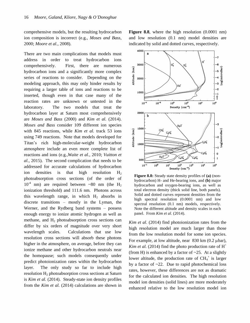
is Kim et al. (2014). Steady-state ion density profiles
from the Kim et al. (2014) calculations are shown in
Figure 8.8, where the high resolution (0.0001 nm)
and low resolution (0.1 nm) model densities are
indicated by solid and dotted curves, respectively.
Figure 8.8: Steady state density profiles of (a) (non-
hydrocarbon) H- and He-bearing ions, and (b) major
hydrocarbon and oxygen-bearing ions, as well as
total electron density (thick solid line, both panels).
Solid and dotted curves represent densities from the
high spectral resolution (0.0001 nm) and low
spectral resolution (0.1 nm) models, respectively.
Note the different altitude and density scales in each
panel. From Kim et al. (2014).
Kim et al. (2014) find photoionization rates from the
high resolution model are much larger than those
from the low resolution model for some ion species.
For example, at low altitude, near 830 km (0.2 bar),
Kim et al. (2014) find the photo production rate of H+
(from H) is enhanced by a factor of ~25. At a slightly
lower altitude, the production rate of CH4+ is larger
by a factor of ~22. Due to rapid photochemical loss
rates, however, these differences are not as dramatic
for the calculated ion densities. The high resolution
model ion densities (solid lines) are more moderately
enhanced relative to the low resolution model ion
Saturn’s Ionosphere 17
densities (dotted lines) in Figure 8.8: the sum of the
ion densities at the hydrocarbon peak is ~3200 cm-3
and ~1800 cm-3
for the high resolution and low
resolution models, respectively.
Plasma temperatures
Ion, electron, and neutral temperatures are expected
to deviate in the upper atmosphere of Saturn, though
no in situ measurements have yet been made.
Photoelectron (and secondary electron) interactions
with the ambient plasma are likely the dominant
source of heating in the non-auroral ionosphere, and
therefore plasma temperature model calculations
require an accurate treatment of the transport, energy
degradation, and angular redistribution of
suprathermal electrons. Plasma temperatures affect
ionospheric model calculations primarily by altering
chemical reaction and ambipolar diffusion rates.
There are two model calculations for plasma
temperatures at Saturn available in the refereed
literature, one at high latitudes (Glocer et al., 2007),
and one at mid latitudes (Moore et al., 2008). (Two
other previous studies are from Ph.D. dissertations:
Waite, 1981; Frey, 1997.)
Glocer et al. (2007) use a 1-D multi-fluid model to
study the polar wind at Saturn, starting from below
the ionospheric peak and extending to an altitude of
1 RS, yielding densities, fluxes, and temperatures for
H+ and H3
+. They find peak ion temperatures of
roughly 2000-3200 K for H+ and 1300-2600 K for
H3+ – well above the main ionosphere sampled by
remote auroral observations. Moore et al. (2008)
self-consistently coupled a 1-D ionospheric model
that solves the ion continuity, momentum, and energy
equations with a suprathermal electron transport code
adapted to Saturn (Galand et al., 2009). Their
calculations specified a fixed neutral background
based on results from 3-D global circulation
calculations that reproduced observed thermospheric
temperatures (Müller-Wodarg et al., 2006). Moore et
al. (2008) found only relatively modest electron
temperature enhancements during the Saturn day,
calculating peak values of ~500-560 K (~80-140 K
above the neutral temperature). Ion temperatures
were somewhat smaller, reaching ~480 K at the
topside during the day while remaining nearly equal
to the neutral temperature at altitudes near and below
the electron density peak. Both ions and electrons
cooled to the neutral temperature within an hour after
sunset. A parameterization of the thermal electron
heating rate based on primary photoionization rates
was also developed (Moore et al., 2008) and then
demonstrated to work for a wide variety of
seasonal/solar conditions and latitudes (Moore et al.,
2009).
Plasma temperatures can also be estimated from the
topside scale heights of observed electron densities,
though there are a number of uncertainties associated
with such an estimate. For example, the ion
composition has not been measured, and there may be
small altitude gradients in temperature. Both of these
unknowns can lead to ambiguous results.
Nonetheless, as most Saturn models predict H+ as the
dominant topside ion, especially at dawn, Nagy et al.
(2006) assumed H+ was the major topside ion and
neglected possible temperature gradients in order to
arrive at an estimate of 625 K based on analyzing the
average low-latitude dawn radio occultation profile
above 2500 km altitude. By applying the same
assumptions, and by considering that dusk
temperatures should be at least as large as dawn
temperatures, Nagy et al. (2006) further arrive at the
implication that the dusk topside might be 72% H3+,
or 7.7% H3O+, or some other appropriate combination
of ion fractions.
8.3.2 Model-Data Comparisons
There are five major categories of observational
constraints that must be explained by models: (1)
peak electron density and altitude, (2) dawn/dusk
electron density asymmetry, (3) latitudinal variations
18 Moore, Galand, Kliore, Nagy & O’Donoghue
in NMAX and TEC, (4) diurnal variation of NMAX, and
(5) latitudinal H3+ structure. While a number of these
observational constraints are closely related, it is
illustrative to review model-data comparisons for
each separately in order to highlight the key
parameters that drive each of the observables.
Models typically attempt to reproduce two or more of
the observables simultaneously, though this is often
not possible due to the different solar, seasonal and
latitudinal conditions of the multi-instrumental
observations.
Electron Density Altitude Structure
Peak electron densities in Saturn’s ionosphere
(NMAX), based on Cassini radio occultations, range
from ~0.3x10³-2.6x10
4 cm
-3 at dawn and
~3x10³-1.9x10
4 at dusk. The altitude of the electron
density peak, hMAX, has been observed at altitudes
between 1100 km and 3200 km (Section 8.2.1). In
general, both hMAX and NMAX are smallest near
Saturn’s equator, and increase with latitude, though
there is significant scatter about this average behavior
(Kliore et al., 2014).
The primary focus of early Saturn ionospheric models
following the observations of the Pioneer and
Voyager spacecraft was on reducing modeled
electron densities to the measured ~104 cm
-3 peak
value. As can be seen from Figure 8.1, there is very
rarely a classic Chapman-type smooth electron
density profile at Saturn, and the maximum electron
density is at times located in a narrow low-altitude
layer rather than what might be called the “main
peak”. For these reasons, models have generally
focused on understanding the average trends revealed
by observations rather than on reproducing exact
electron density altitude profiles. Individual profiles
have also been reproduced in the past, typically by
varying a number of free parameters (e.g., Majeed
and McConnell, 1991): the population of
vibrationally excited H2, the external water influx,
and the vertical plasma drift. The first two of these
parameters have been discussed already (Section
8.3.1); vertical plasma drift can arise from neutral
winds (e.g., meridional winds driving plasma up or
down magnetic field lines) and electric fields (e.g.,
E x B drifts driven by zonal electric fields; Kelley,
2009; Schunk and Nagy, 2009). Whereas the primary
effect of an enhanced population of vibrationally
excited H2 or water influx is to reduce the modeled
electron densities, the peak altitude is also slightly
increased as these reactions are more effective at
lower altitudes (e.g., Majeed and McConnell, 1991;
Moses and Bass, 2000; Moore et al., 2004).
Similarly, the primary effect of a vertical plasma drift
is to shift hMAX up or down in altitude, though NMAX
can also be affected if the plasma is moved into a
different chemical or dynamical regime.
Though it is possible to construct a model
reproduction of most of the observed electron density
altitude profiles by exploring unknown parameters
(though likely not all of them), the derived
parameters vary significantly from observation to
observation. No single set of water influxes,
vibrationally excited H2 populations, and enforced
vertical plasma drifts can reproduce all of the
observed radio occultation electron densities
simultaneously, possibly indicating spatial and
temporal variations in these parameters.
Beyond simply comparing to NMAX and hMAX,
modelers have also attempted to understand the
narrow layers of electron density frequently observed
(Figures 8.1-8.2). Vertically varying horizontal
winds, such as might occur from atmospheric gravity
waves, can cause alternating compression and
extension of plasma with altitude, thus creating
ionospheric layers (Kelley, 2009). Such layering is
frequently observed in the terrestrial E region and the
lower F region. This mechanism is especially
effective for long lived ions, such as the metallic ions
introduced from the ablation of micrometeoroids.
Moses and Bass (2000) were able to demonstrate the
plausibility of such a layering process in Saturn’s
ionosphere by introducing a modest oscillatory
vertical plasma drift as well as a Mg influx of
Saturn’s Ionosphere 19
1.3x105 cm
-2 s
-1 focused in the 790-1290 km region.
Kim et al. (2014) also suggest that such layers may
result from photochemistry driven by high resolution
H2 photoabsorption cross sections.
Based on a wavelet analysis of 31 Cassini radio
occultations (Nagy et al., 2006; Kliore et al., 2009),
Matcheva and Barrow (2012) were able to detect
several discrete scales of variability in Saturn’s
electron density profiles. Furthermore, by applying a
gravity wave propagation model to Saturn’s upper
atmosphere, they also demonstrated that the observed
features were consistent with gravity waves being
present in the lower ionosphere, causing layering of
the ions and electrons. In a continuation of that
study, wherein a 2-D, non-linear, time-dependent
model of the interaction of atmospheric gravity waves
with ionospheric ions was applied to Saturn’s upper
atmosphere, Barrow and Matcheva (2013) were able
to reproduce the structure of two Cassini radio
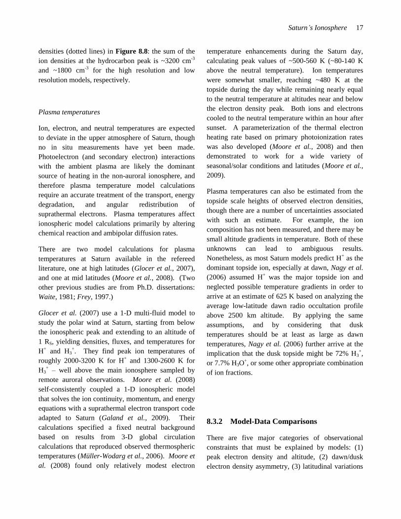
occultations, the S08 entry and the S56 exit.
Figure 8.9 presents the model-data comparison for
the S56 occultation.
Figure 8.9: Comparison between the S56 exit
observation (black line) and a model electron density
profile (red line). The ionospheric model illustrates
the effect of three small-amplitude gravity waves
superimposed on the background electron density
profile. From Barrow and Matcheva (2013).
Extreme “bite-outs”, or localized electron density
depletions, frequently seen in Saturn radio
occultations, can also be produced from atmospheric
gravity waves, as discussed above (see also Figure 6
of Kliore et al., 2009). Another possible generation
mechanism for ionospheric depletions is a time-
dependent water influx. Moore and Mendillo (2007)
were able to reproduce the observed S7 bite-out by
increasing the background water influx (of
5x106 cm
-2 s
-1) by a factor of 50 for ~27 minutes, after
which it returned to its initial value. As the resulting
bulge of water density diffuses downward through the
thermosphere, it undergoes charge exchange reactions
with H+, leading to a localized reduction in electron
density. While a number of Cassini radio
occultations contain depletions similar to the Moore
and Mendillo (2007) results, the magnitude and
frequency of possible water influx variations are not
known at present. Therefore this possibility remains
unconfirmed. Nevertheless, atmospheric gravity
waves have difficulty producing ionospheric structure
at high altitude due to wave dissipation lower in the
thermosphere (Matcheva and Barrow, 2012), and as
some electron density depletions have been observed
above 2000 km (Kliore et al., 2009), an alternative
mechanism for generating such structures, such as a
time-variable water influx, may yet be required to
reproduce some observed electron density altitude
profiles.
Dawn/Dusk Electron Density Asymmetry
The first dozen radio occultations obtained by Cassini
revealed a dawn/dusk asymmetry in Saturn’s low-
latitude ionosphere (Nagy et al., 2006). On average
the peak densities are lower and the peak altitudes
higher at dawn than at dusk. A recently developed
global circulation model (GCM) of Saturn’s upper
atmosphere, called STIM (the Saturn Thermosphere
Ionosphere Model), was leveraged in order to study
this new observational constraint. In comparing with
the first dozen Cassini equatorial radio occultations,
1-D ionospheric calculations were performed (Moore
et al., 2006) using a 3-D thermosphere that
reproduced observed upper atmospheric temperatures
using a combination of auroral Joule heating and low-

20 Moore, Galand, Kliore, Nagy & O’Donoghue
latitude wave heating (Müller-Wodarg et al., 2006).
Moore et al. (2006) found that the average dawn and
dusk equatorial electron density profiles were best
reproduced by model simulations that considered a
water influx at the top of the atmosphere of
5x106 cm
-2 s
-1. Electron density comparisons are
shown in Figure 8.10. This water influx was roughly
a factor of three larger than the globally averaged
influx derived from ISO observations,
1.5x106 cm
-2 s
-1 (Moses et al., 2000), though such a
difference is likely not drastic enough to conflict with
the spatial constraints evaluated by Moses et al.
(2000). The fact that the Moore et al. (2006) water
influx is smaller than the favored value derived from
previous comparisons with the Voyager 2 exit
occultation, 2.2x107 cm
-2 s
-1 (Majeed and McConnell,
1991), can be explained by the fact that the Majeed
and McConnell (1991) water influx was derived for a
scenario in which electron loss due to reactions
between protons and vibrationally excited H2 was not
considered. By including this reaction in addition to
charge exchange with water, the magnitude of each
required rate is reduced: Moore et al. (2006) favored
a population of vibrationally excited H2 that was 25%
the nominal value considered by Majeed and
McConnell (1991).
Figure 8.10: The average (a) dawn and (b) dusk Cassini electron density profiles (Nagy et al., 2006) along with
model comparisons. Dotted lines represent model results that best match the observations at both dusk and dawn
using a full diurnal calculation with a single set of parameters, whereas dashed and dot-dashed lines give results best
matched to the average dawn or dusk profile, respectively. The width of the shaded regions corresponds to the full
range of electron densities observed by Cassini, and the degree of shading represents three distinct ionospheric
altitude regimes, from top to bottom: diffusive regime (dominated by H+), photochemical regime (dominated by H
+
and H3+), and hydrocarbon/metallic ion regime (where these ions begin to dominate). From Moore et al. (2006).
The diurnal variation in peak electron density implied
by the model reproductions of average dawn and dusk
Cassini occultations was modest, less than a factor of
6, as illustrated in Figure 8.11. A similar set of
parameters was able to reproduce the dawn and dusk
NMAX values measured by Cassini for a majority of
the twelve equatorial occultations, with the notable
exceptions being S11x, S9x, and S12n/x (Moore et
al., 2006).
The dawn/dusk asymmetry is primarily due to the
presence of both atomic (H+) and molecular (H3
+)
ions at the electron density peak. At dusk the solar
source of ionization has only just shut off, so both H+
and H3+ are still present and contribute to the electron
density peak. During the ~5 hours of darkness on the
nightside, however, most of the H3+ ions have
dissociatively recombined with electrons, resulting in
a reduced electron density at dawn. This effect is

Saturn’s Ionosphere 21
similar to another well-known atomic and molecular
ion region, the terrestrial F-layer. Modeled ion and
electron altitude profiles at dawn, noon, and dusk, are
presented in Figure 8.12, demonstrating the loss of
H3+ ions during the Saturn night (Moore et al., 2008).
Earlier Saturn ionospheric calculations produce the
same sort of variations in H3+, H
+, and Ne, though for
different seasonal and solar conditions (e.g., Figure 6
of Majeed and McConnell, 1996; Figure 13 of Moses
and Bass, 2000).
Figure 8.11: Plot of modeled local time variations
of NMAX. Each solid line represents the best diurnal
match for one set of combinations of the two
unknown chemical losses (due to vibrationally
excited H2 and water influx). Gray shaded
rectangles identify the ranges in local solar time and
NMAX from the Cassini radio occultations (Nagy et
al., 2006). Numbers and arrows mark the individual
occultation values and “x” marks the averaged dawn
and dusk observations. From Moore et al. (2006).
Latitudinal Variations in NMAX and TEC
Analysis of 19 additional Cassini radio occultations
mostly at mid- and high-latitudes (Kliore et al.,
2009), in addition to the 12 previous equatorial
occultations (Nagy et al., 2006), revealed a clear
latitudinal trend in electron density: on average,
electron densities were smallest at Saturn’s equator
and increased with latitude. This trend was recently
strengthened by the addition of 28 more radio
occultations across all latitudes (Figure 8.3; Kliore et
al., 2014). The sub-solar point was near Saturn’s
equator for a majority of the occultations, and
therefore the presence of a minimum in electron
density in the region of peak photoionization was
most likely indicative of a latitudinal dependence in
the chemical loss rates.
Moore et al. (2010) explored the possibility of a
latitudinally varying chemical loss using 2-D
ionospheric calculations combined with a fixed 3-D
thermospheric background appropriate for the
average seasonal and solar conditions for the first 31
Cassini radio occultations (Kliore et al., 2009). They
evaluated a Gaussian water influx centered at
Saturn’s equator with a peak value of
(0.1-1)x107 cm
-2 s
-1 and a full width half maximum
(FWHM) between 2o-180
o (in addition to a
latitudinally invariant water influx). Six populations
of vibrationally excited H2 were also considered,
based on modifications to the Majeed et al. (1991)
values by a factor of 0-2. The observed latitudinal
trend in electron density was best reproduced for a
Gaussian water influx centered at the equator with a
FWHM of ~23.5o, illustrated in the left panel of
Figure 8.13. The globally averaged water influx
from such a profile is 1.1x106 cm
-2 s
-1, slightly less
than the 1.5x106 cm
-2 s
-1 inferred from ISO
measurements (Moses et al., 2000; Moore et al.,
2015).
Müller-Wodarg et al. (2012) applied the Moore et al.
(2010) water distribution in a subsequent study
focused on magnetosphere-atmosphere coupling at
high latitudes using the full 3-D STIM. Figure 8.13
illustrates the imposed water influx and the latitude
variation of both modeled and observed electron
densities with latitude, demonstrating that a
combination of latitudinally varying water influxes
and seasonal trends can explain the majority of NMAX
variations from radio occultation observations.
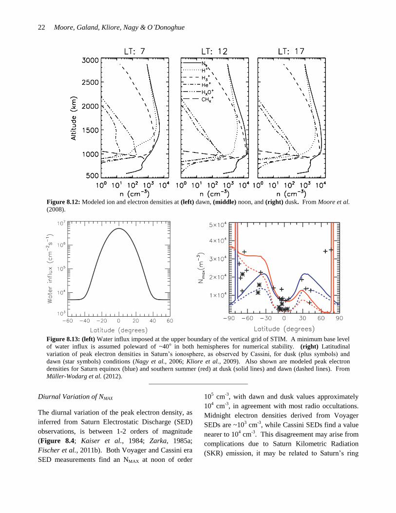
22 Moore, Galand, Kliore, Nagy & O’Donoghue
Figure 8.12: Modeled ion and electron densities at (left) dawn, (middle) noon, and (right) dusk. From Moore et al.
(2008).
Figure 8.13: (left) Water influx imposed at the upper boundary of the vertical grid of STIM. A minimum base level
of water influx is assumed poleward of ~40o in both hemispheres for numerical stability. (right) Latitudinal
variation of peak electron densities in Saturn’s ionosphere, as observed by Cassini, for dusk (plus symbols) and
dawn (star symbols) conditions (Nagy et al., 2006; Kliore et al., 2009). Also shown are modeled peak electron
densities for Saturn equinox (blue) and southern summer (red) at dusk (solid lines) and dawn (dashed lines). From
Müller-Wodarg et al. (2012).
Diurnal Variation of NMAX
The diurnal variation of the peak electron density, as
inferred from Saturn Electrostatic Discharge (SED)
observations, is between 1-2 orders of magnitude
(Figure 8.4; Kaiser et al., 1984; Zarka, 1985a;
Fischer et al., 2011b). Both Voyager and Cassini era
SED measurements find an NMAX at noon of order
105 cm
-3, with dawn and dusk values approximately
104 cm
-3, in agreement with most radio occultations.
Midnight electron densities derived from Voyager
SEDs are ~103 cm
-3, while Cassini SEDs find a value
nearer to 104 cm
-3. This disagreement may arise from
complications due to Saturn Kilometric Radiation
(SKR) emission, it may be related to Saturn’s ring
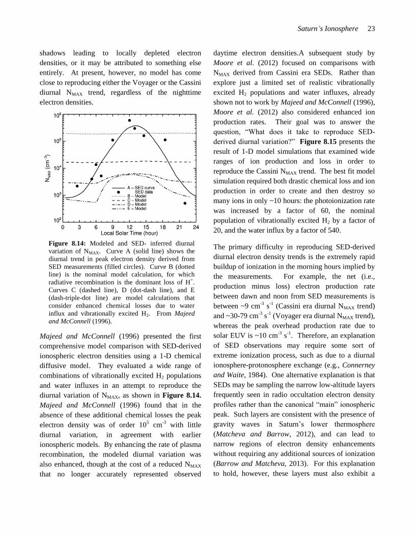
Saturn’s Ionosphere 23
shadows leading to locally depleted electron
densities, or it may be attributed to something else
entirely. At present, however, no model has come
close to reproducing either the Voyager or the Cassini
diurnal NMAX trend, regardless of the nighttime
electron densities.
Figure 8.14: Modeled and SED- inferred diurnal
variation of NMAX. Curve A (solid line) shows the
diurnal trend in peak electron density derived from
SED measurements (filled circles). Curve B (dotted
line) is the nominal model calculation, for which
radiative recombination is the dominant loss of H+.
Curves C (dashed line), D (dot-dash line), and E
(dash-triple-dot line) are model calculations that
consider enhanced chemical losses due to water
influx and vibrationally excited H2. From Majeed
and McConnell (1996).
Majeed and McConnell (1996) presented the first
comprehensive model comparison with SED-derived
ionospheric electron densities using a 1-D chemical
diffusive model. They evaluated a wide range of
combinations of vibrationally excited H2 populations
and water influxes in an attempt to reproduce the
diurnal variation of NMAX, as shown in Figure 8.14.
Majeed and McConnell (1996) found that in the
absence of these additional chemical losses the peak
electron density was of order 105 cm
-3 with little
diurnal variation, in agreement with earlier
ionospheric models. By enhancing the rate of plasma
recombination, the modeled diurnal variation was
also enhanced, though at the cost of a reduced NMAX
that no longer accurately represented observed
daytime electron densities.A subsequent study by
Moore et al. (2012) focused on comparisons with
NMAX derived from Cassini era SEDs. Rather than
explore just a limited set of realistic vibrationally
excited H2 populations and water influxes, already
shown not to work by Majeed and McConnell (1996),
Moore et al. (2012) also considered enhanced ion
production rates. Their goal was to answer the
question, “What does it take to reproduce SED-
derived diurnal variation?” Figure 8.15 presents the
result of 1-D model simulations that examined wide
ranges of ion production and loss in order to
reproduce the Cassini NMAX trend. The best fit model
simulation required both drastic chemical loss and ion
production in order to create and then destroy so
many ions in only ~10 hours: the photoionization rate
was increased by a factor of 60, the nominal
population of vibrationally excited H2 by a factor of
20, and the water influx by a factor of 540.
The primary difficulty in reproducing SED-derived
diurnal electron density trends is the extremely rapid
buildup of ionization in the morning hours implied by
the measurements. For example, the net (i.e.,
production minus loss) electron production rate
between dawn and noon from SED measurements is
between ~9 cm-3
s-1
(Cassini era diurnal NMAX trend)
and ~30-79 cm-3
s-1
(Voyager era diurnal NMAX trend),
whereas the peak overhead production rate due to
solar EUV is ~10 cm-3
s-1
. Therefore, an explanation
of SED observations may require some sort of
extreme ionization process, such as due to a diurnal
ionosphere-protonosphere exchange (e.g., Connerney
and Waite, 1984). One alternative explanation is that
SEDs may be sampling the narrow low-altitude layers
frequently seen in radio occultation electron density
profiles rather than the canonical “main” ionospheric
peak. Such layers are consistent with the presence of
gravity waves in Saturn’s lower thermosphere
(Matcheva and Barrow, 2012), and can lead to
narrow regions of electron density enhancements
without requiring any additional sources of ionization
(Barrow and Matcheva, 2013). For this explanation
to hold, however, these layers must also exhibit a
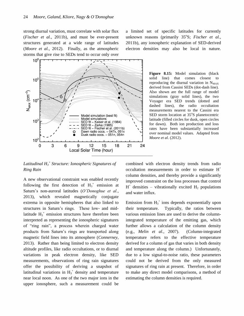
24 Moore, Galand, Kliore, Nagy & O’Donoghue
strong diurnal variation, must correlate with solar flux
(Fischer et al., 2011b), and must be ever-present
structures generated at a wide range of latitudes
(Moore et al., 2012). Finally, as the atmospheric
storms that give rise to SEDs tend to occur only over
a limited set of specific latitudes for currently
unknown reasons (primarily 35oS; Fischer et al.,
2011b), any ionospheric explanation of SED-derived
electron densities may also be local in nature.
Figure 8.15: Model simulation (black
solid line) that comes closest to
reproducing the diurnal variation in NMAX
derived from Cassini SEDs (dot-dash line).
Also shown are the full range of model
simulations (gray solid lines), the two
Voyager era SED trends (dotted and
dashed lines), the radio occultation
measurements nearest to the Cassini era
SED storm location at 35oS planetocentric
latitude (filled circles for dusk, open circles
for dawn). Both ion production and loss
rates have been substantially increased
over nominal model values. Adapted from
Moore et al. (2012).
Latitudinal H3+ Structure: Ionospheric Signatures of
Ring Rain
A new observational constraint was enabled recently
following the first detection of H3+ emission at
Saturn’s non-auroral latitudes (O’Donoghue et al.,
2013), which revealed magnetically conjugate
extrema in opposite hemispheres that also linked to
structures in Saturn’s rings. These low- and mid-
latitude H3+ emission structures have therefore been
interpreted as representing the ionospheric signatures
of “ring rain”, a process wherein charged water
products from Saturn’s rings are transported along
magnetic field lines into its atmosphere (Connerney,
2013). Rather than being limited to electron density
altitude profiles, like radio occultations, or to diurnal
variations in peak electron density, like SED
measurements, observations of ring rain signatures
offer the possibility of deriving a snapshot of
latitudinal variations in H3+ density and temperature
near local noon. As one of the two major ions in the
upper ionosphere, such a measurement could be
combined with electron density trends from radio
occultation measurements in order to estimate H+
column densities, and thereby provide a significantly
improved constraint on the loss processes that control
H+ densities – vibrationally excited H2 populations
and water influx.
Emission from H3+ ions depends exponentially upon
their temperature. Typically, the ratios between
various emission lines are used to derive the column-
integrated temperature of the emitting gas, which
further allows a calculation of the column density
(e.g., Melin et al., 2007). (Column-integrated
temperature refers to the effective temperature
derived for a column of gas that varies in both density
and temperature along the column.) Unfortunately,
due to a low signal-to-noise ratio, these parameters
could not be derived from the only measured
signatures of ring rain at present. Therefore, in order
to make any direct model comparisons, a method of
estimating the column densities is required.

Saturn’s Ionosphere 25
In a recent study involving 1-D ionospheric
calculations over a fixed 3-D background
thermosphere, Moore et al. (2015) addressed this
shortcoming by first estimating the neutral
temperatures. They based latitudinal trends in
exospheric temperature on solar and stellar EUV
occultation results described in Chapter 9. As these
temperatures represent conditions near the top of the
atmosphere, above the altitude of peak H3+ ionization,
an offset was then applied that accounted for the
difference in neutral temperature between H3+
altitudes and the exobase as a function of latitude, as
calculated by the 3-D STIM (Müller-Wodarg et al.,
2012). These temperature estimates were then
combined with the measured intensities in order to
derive H3+ column densities from the observations,
shown in Figure 8.16. The structure in Figure 8.16
is driven by the observed structure in H3+ emission,
whereas the range of estimated column densities is
dominated by temperature uncertainties.
Figure 8.16: Maximum H3+ column densities estimated from Saturn observations of ring rain signatures
(O’Donoghue et al., 2013), based on exospheric temperature measurements (Koskinen et al., 2013) and modeled
temperature offsets (Müller-Wodarg et al., 2012). The range of H3+ column densities is driven primarily by
temperature uncertainties of ~80 K. Adapted from Moore et al. (2015).
While enhanced populations of vibrationally excited
H2 and water influxes have historically been
considered as a means of reducing the modeled
electron density (via destruction of the long-lived H+
ions), there is an important secondary effect on H3+
densities. Specifically, as the dominant chemical loss
for H3+ in outer planet ionospheres is due to
dissociative recombination with electrons, the above
loss processes also act as proxy “sources” of H3+ by
reducing its dissociative recombination rate in
correspondence with the reduced electron densities.
This effect is augmented without limit by reactions
between H+ and vibrationally excited H2, as they lead
to additional production of H2+ (and therefore H3
+),
but it is reversed for water influxes above
~107 cm
-2 s
-1, as H3
+ can also be lost due to charge
exchange with water products (Moore et al., 2015).
Contours of H3+ column density as a function of
vibrationally excited H2 population (designated as
kfac) and water influx are presented in Figure 8.17. A
dashed contour indicates the estimated column
density, and therefore represents the combinations of
kfac and 𝜙𝐻2𝑂 that could reproduce the observation at
that latitude, 35oS planetocentric. By performing a
similar series of calculations for each of the 40
latitude elements of the observations, Moore et al.
(2015) were able to derive a latitudinal variation in
the maximum water influxes and maximum
populations of vibrationally excited H2. They
estimated the globally averaged maximum ring-
derived water influx to be (1.6-12)x105 cm
-2 s
-1,
which represents a maximum total global influx of
water from Saturn’s rings to its atmosphere of
(1.0-6.8)x1026
s-1
. While there are no direct
observational constraints for purely ring-derived

26 Moore, Galand, Kliore, Nagy & O’Donoghue
water influxes, these upper limits compare favorably
with the total oxygen influx of ~105 cm
-2 s
-1 estimated
from ring atmosphere models (e.g., Tseng et al.,
2010). Furthermore, the globally averaged upper
limits for water influx, when combined with the
assumed neutral water influx profile of Figure 8.13,
are (1.3-2.3)x106 cm
-2 s
-1, fairly close to the value of
~1.5x106 cm
-2 s
-1 derived by Moses et al. (2000)
based on ISO observations (Feuchtgruber et al.,
1997). The wide ranges in these estimates stem
primarily from uncertainties in H3+ column integrated
temperatures, and therefore future observations of the
ionospheric signatures of ring rain may be able to
reduce those uncertainties by determining
temperatures self-consistently.
Figure 8.17: Contours of modeled H3+ column densities for a range of water influxes, 𝜙𝐻2𝑂, and populations of
vibrationally excited H2 (represented as kfac). Calculation results are for 35oS planetocentric latitude at local solar
noon. The dashed curves indicate the H3+ column density estimated from the observations (Figure 8.16), and
therefore identify combinations of 𝜙𝐻2𝑂 and kfax that can reproduce the observation at that latitude. Dotted curves
outline a range of H3+ column densities that result from accounting for a 3 uncertainty in the observed emission
intensity. From Moore et al. (2015).
8.4 Summary
Saturn ionospheric science has advanced significantly
over the past decade. Prior to the arrival of Cassini,
there were 6 electron density profiles from radio
occultations – there are now a total of 65. The
diurnal variation in peak electron density derived
from Voyager era Saturn Electrostatic Discharge
(SED) measurements was based on a few
measurements over three SED episodes. In contrast,
Cassini era diurnal variations of electron density were
derived from 48 SED episodes by 2009, and there is a
corresponding wider range of additional
observational parameters to explore (e.g., Cassini
distance from Saturn versus derived electron density).
In addition, there is the promise of a new remote
observational constraint for Saturn’s mid- and low-
latitudes: H3+ emissions and related ring rain
implications. While the conclusions that can be
drawn from the current measurements of ring rain
signatures are not yet definitive, future observations

Saturn’s Ionosphere 27
should allow derivations of H3+ and H
+ column
densities, column-integrated H3+ temperatures, and an
in depth examination of the coupling between
Saturn’s rings and its atmosphere.
Ionospheric models are able to explain the gross
ionospheric structure revealed by radio occultation
measurements. Electron densities appear to be
controlled primarily by a latitudinally varying water
influx, reducing the need for enhanced populations of
vibrationally excited molecular hydrogen. The
observed dawn/dusk asymmetry is well explained by
a mix of atomic (H+) and molecular (H3
+) ions
forming Saturn’s main ionospheric peak. Low-
altitude layers are likely indicative of atmospheric
gravity waves, which can lead to vertically varying
plasma drifts.
The major remaining model-data discrepancy is in the
diurnal variation of peak electron density. SED-
derived electron densities feature large daytime
values and strong diurnal variations. Models can
reproduce one or the other of these constraints, but
not both simultaneously, having thoroughly
demonstrated that no combination of known
chemistry can account for the SED-derived
variations. Resolution of this discrepancy may lie in
introducing additional dynamics to the modeling,
such as a diurnal ionosphere-protonosphere exchange,
or further investigation into the possibility that SEDs
are sampling the narrow low-altitude layers of
electron density, or something else entirely.
Future observations should help refine the modeling
constraints in a number of important areas.
Observations of ionospheric H3+ emissions can
provide the first ion density and temperature
measurements in Saturn’s ionosphere. Additional
insights into ion densities resulting from in situ
measurements are expected during Cassini’s end-of-
mission proximal orbits in 2017. During this mission
phase, called the Cassini Grand Finale, the spacecraft
will sample Saturn’s upper atmosphere directly,
dipping below 2000 km altitude on 22 orbits, with
periapse at low latitude near dusk. With luck, Cassini
may also be able to measure near-Saturn SEDs or
determine the properties of the particles on magnetic
field lines connecting Saturn’s rings to its
atmosphere. Combined with the existing
observational constraints, these two new datasets –
ground-based observations and Cassini Grand Finale
measurements – should help to refine the remaining
model-data discrepancies and to pave the way for
future fully coupled models of the Saturn system by
providing much needed insight into ionospheric
chemical losses due to water and to vibrationally
excited H2.
Acknowledgements
The authors wish to acknowledge the contribution of
the International Space Sciences Institute (ISSI) in
Bern, Switzerland, for hosting and funding the
International Team on “Coordinated Numerical
Modeling of the Global Jovian and Saturnian
Systems”, and the constructive discussions by
colleagues attending the meetings. The manuscript
benefitted significantly from thorough reviews by two
anonymous reviewers. Support for this work at
Boston University comes from NASA Grants
NNX13AG21G, NNX13AG57G, and
NNX14AG72G. M.G. was supported by the STFC of
UK under grant ST/K001051/1 and ST/N000692/1.
A.F.N. acknowledges support from the Cassini
Mission as a member of the Radio Science Team.
Arvydas J. Kliore
This chapter is dedicated to the memory of Arvydas J.
Kliore, a pioneer in the field of Radio Science. He
was involved in spacecraft radio occultations from
the very first NASA planetary mission, and has
shaped our knowledge of Saturn’s upper atmosphere
in his role as Principle Investigator of the Cassini
Radio Science Subsystem. Without him, this chapter
would not exist.
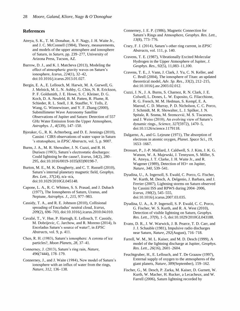
28 Moore, Galand, Kliore, Nagy & O’Donoghue
References
Atreya, S. K., T. M. Donahue, A. F. Nagy, J. H. Waite Jr.,
and J. C. McConnell (1984), Theory, measurements,
and models of the upper atmosphere and ionosphere
of Saturn, in Saturn, pp. 239–277, University of
Arizona Press, Tucson, AZ.
Barrow, D. J., and K. I. Matcheva (2013), Modeling the
effect of atmospheric gravity waves on Saturn’s
ionosphere, Icarus, 224(1), 32–42,
doi:10.1016/j.icarus.2013.01.027.
Bergin, E. A., E. Lellouch, M. Harwit, M. A. Gurwell, G.
J. Melnick, M. L. N. Ashby, G. Chin, N. R. Erickson,
P. F. Goldsmith, J. E. Howe, S. C. Kleiner, D. G.
Koch, D. A. Neufeld, B. M. Patten, R. Plume, R.
Schieder, R. L. Snell, J. R. Stauffer, V. Tolls, Z.
Wang, G. Winnewisser, and Y. F. Zhang (2000),
Submillimeter Wave Astronomy Satellite
Observations of Jupiter and Saturn: Detection of 557
GHz Water Emission from the Upper Atmosphere,
Astrophys. J., 4(539), 147–150.
Bjoraker, G., R. K. Achterberg, and D. E. Jennings (2010),
Cassini / CIRS observations of water vapor in Saturn
’s stratosphere, in EPSC Abstracts, vol. 5, p. 9007.
Burns, J. A., M. R. Showalter, J. N. Cuzzi, and R. H.
Durisen (1983), Saturn’s electrostatic discharges:
Could lightning be the cause?, Icarus, 54(2), 280–
295, doi:10.1016/0019-1035(83)90198-7.
Burton, M. E., M. K. Dougherty, and C. T. Russell (2010),
Saturn’s internal planetary magnetic field, Geophys.
Res. Lett., 37(24), n/a–n/a,
doi:10.1029/2010GL045148.
Capone, L. A., R. C. Whitten, S. S. Prasad, and J. Dubach
(1977), The Ionospheres of Saturn, Uranus, and
Neptune, Astrophys. J., 215, 977–983.
Cassidy, T. A., and R. E. Johnson (2010), Collisional
spreading of Enceladus’ neutral cloud, Icarus,
209(2), 696–703, doi:10.1016/j.icarus.2010.04.010.
Cavalié, T., V. Hue, P. Hartogh, E. Lellouch, T. Cassidy,
M. Dobrijevic, C. Jarchow, and R. Moreno (2014), Is
Enceladus Saturn’s source of water?, in EPSC
Abstracts, vol. 9, p. 411.
Chen, R. H. (1983), Saturn’s ionosphere: A corona of ice
particles?, Moon Planets, 28, 37–41.
Connerney, J. (2013), Saturn’s ring rain, Nature,
496(7444), 178–179.
Connerney, J., and J. Waite (1984), New model of Saturn’s
ionosphere with an influx of water from the rings,
Nature, 312, 136–138.
Connerney, J. E. P. (1986), Magnetic Connection for
Saturn’s Rings and Atmosphere, Geophys. Res. Lett.,
13(8), 773–776.
Crary, F. J. (2014), Saturn’s other ring current, in EPSC
Abstracts, vol. 111, p. 140.
Cravens, T. E. (1987), Vibrationally Excited Molecular
Hydrogen in the Upper Atmosphere of Jupiter, J.
Geophys. Res., 92(5), 11,083–11,100.
Cravens, T. E., J. Vann, J. Clark, J. Yu, C. N. Keller, and
C. Brull (2004), The ionosphere of Titan: an updated
theoretical model, Adv. Sp. Res., 33(2), 212–215,
doi:10.1016/j.asr.2003.02.012.
Cuzzi, J. N., J. A. Burns, S. Charnoz, R. N. Clark, J. E.
Colwell, L. Dones, L. W. Esposito, G. Filacchione,
R. G. French, M. M. Hedman, S. Kempf, E. A.
Marouf, C. D. Murray, P. D. Nicholson, C. C. Porco,
J. Schmidt, M. R. Showalter, L. J. Spilker, J. N.
Spitale, R. Srama, M. Sremcević, M. S. Tiscareno,
and J. Weiss (2010), An evolving view of Saturn’s
dynamic rings., Science, 327(5972), 1470–5,
doi:10.1126/science.1179118.
Dalgarno, A., and G. Lejeune (1971), The absorption of
electrons in atomic oxygen, Planet. Space Sci., 19,
1653–1667.
Drossart, P., J.-P. Maillard, J. Caldwell, S. J. Kim, J. K. G.
Watson, W. A. Majewski, J. Tennyson, S. Miller, S.
K. Atreya, J. T. Clarke, J. H. Waite Jr., and R.
Wagener (1989), Detection of H3+ on Jupiter,
Nature, 340, 539–541.
Dyudina, U., A. Ingersoll, S. Ewald, C. Porco, G. Fischer,
W. Kurth, M. Desch, A. Delgenio, J. Barbara, and J.
Ferrier (2007), Lightning storms on Saturn observed
by Cassini ISS and RPWS during 2004–2006,
Icarus, 190(2), 545–555,
doi:10.1016/j.icarus.2007.03.035.
Dyudina, U. A., A. P. Ingersoll, S. P. Ewald, C. C. Porco,
G. Fischer, W. S. Kurth, and R. A. West (2010),
Detection of visible lightning on Saturn, Geophys.
Res. Lett., 37(9), 1–5, doi:10.1029/2010GL043188.
Evans, D. R., J. W. Warwick, J. B. Pearce, T. D. Carr, and
J. J. Schauble (1981), Impulsive radio discharges
near Saturn, Nature, 292(August), 716–718.
Farrell, W. M., M. L. Kaiser, and M. D. Desch (1999), A
model of the lightning discharge at Jupiter, Geophys.
Res. Lett., 26(16), 2601–2604.
Feuchtgruber, H., E. Lellouch, and T. De Graauw (1997),
External supply of oxygen to the atmospheres of the
giant planets, Nature, 389(September), 159–162.
Fischer, G., M. Desch, P. Zarka, M. Kaiser, D. Gurnett, W.
Kurth, W. Macher, H. Rucker, a Lecacheux, and W.
Farrell (2006), Saturn lightning recorded by
Saturn’s Ionosphere 29
Cassini/RPWS in 2004, Icarus, 183(1), 135–152,
doi:10.1016/j.icarus.2006.02.010.
Fischer, G., D. A. Gurnett, W. S. Kurth, F. Akalin, P.
Zarka, U. A. Dyudina, W. M. Farrell, and M. L.
Kaiser (2008), Atmospheric Electricity at Saturn,
Space Sci. Rev., 137(1-4), 271–285,
doi:10.1007/s11214-008-9370-z.
Fischer, G., W. S. Kurth, D. A. Gurnett, P. Zarka, U. A.
Dyudina, A. P. Ingersoll, S. P. Ewald, C. C. Porco,
A. Wesley, C. Go, and M. Delcroix (2011a), A giant
thunderstorm on Saturn., Nature, 475(7354), 75–7,
doi:10.1038/nature10205.
Fischer, G., D. A. Gurnett, P. Zarka, L. Moore, and U. A.
Dyudina (2011b), Peak electron densities in Saturn’s
ionosphere derived from the low-frequency cutoff of
Saturn lightning, J. Geophys. Res., 116(A4),
A04315, doi:10.1029/2010JA016187.
Fjeldbo, G., A. Kliore, and V. Eshleman (1971), The
neutral atmosphere of Venus as studied with the
Mariner V radio occultation experiements, Astron. J.
Fjeldbo, G., A. Kliore, B. Seidel, D. Sweetnam, and D.
Cain (1975), The Pioneer 10 radio occultation
measurements of the ionosphere of Jupiter, Astron.
Astrophys., 39, 91–96.
Fleshman, B. L., P. A. Delamere, F. Bagenal, and T.
Cassidy (2012), The roles of charge exchange and
dissociation in spreading Saturn’s neutral clouds, J.
Geophys. Res., 117(E5), E05007,
doi:10.1029/2011JE003996.
Fox, J. L. (2004), Response of the Martian
thermosphere/ionosphere to enhanced fluxes of solar
soft X rays, J. Geophys. Res. Sp. Phys., 109(A11), 1–
18, doi:10.1029/2004JA010380.
Fox, J. L. (2007), Near-terminator Venus ionosphere: How
Chapman-esque?, J. Geophys. Res., 112(E4),
E04S02, doi:10.1029/2006JE002736.
Fox, J. L., and K. E. Yeager (2006), Morphology of the
near-terminator Martian ionosphere: A comparison
of models and data, J. Geophys. Res., 111(A10),
A10309, doi:10.1029/2006JA011697.
Frey, M. A. (1997), The polar wind of Saturn, University
of Michigan.
Galand, M., R. V. Yelle, a. J. Coates, H. Backes, and J.-E.
Wahlund (2006), Electron temperature of Titan’s
sunlit ionosphere, Geophys. Res. Lett., 33(21),
L21101, doi:10.1029/2006GL027488.
Galand, M., L. Moore, B. Charnay, I. Mueller-Wodarg,
and M. Mendillo (2009), Solar primary and
secondary ionization at Saturn, J. Geophys. Res.,
114(A6), A06313, doi:10.1029/2008JA013981.
Galand, M., L. Moore, I. Mueller-Wodarg, M. Mendillo,
and S. Miller (2011), Response of Saturn’s auroral
ionosphere to electron precipitation: Electron
density, electron temperature, and electrical
conductivity, J. Geophys. Res., 116(A9), A09306,
doi:10.1029/2010JA016412.
Glocer, A., T. I. Gombosi, G. Toth, K. C. Hansen, A. J.
Ridley, and A. Nagy (2007), Polar wind outflow
model: Saturn results, J. Geophys. Res., 112(A1),
A01304, doi:10.1029/2006JA011755.
Gustin, J., J.-C. Gérard, W. Pryor, P. D. Feldman, D.
Grodent, and G. Holsclaw (2009), Characteristics of
Saturn’s polar atmosphere and auroral electrons
derived from HST/STIS, FUSE and Cassini/UVIS
spectra, Icarus, 200(1), 176–187,
doi:10.1016/j.icarus.2008.11.013.
Hallett, J. T., D. E. Shemansky, and X. Liu (2005a), A
Rotational Level Hydrogen Physical Chemistry
Model for General Astrophysical Application,
Astrophys. J., 624(1), 448–461, doi:10.1086/428935.
Hallett, J. T., D. E. Shemansky, and X. Liu (2005b), Fine-
structure physical chemistry modeling of Uranus H2
X quadrupole emission, Geophys. Res. Lett., 32(2),
L02204, doi:10.1029/2004GL021327.
Hartogh, P., E. Lellouch, R. Moreno, D. Bockelée-Morvan,
N. Biver, T. Cassidy, M. Rengel, C. Jarchow, T.
Cavalié, J. Crovisier, F. P. Helmich, and M. Kidger
(2011), Direct detection of the Enceladus water torus
with Herschel, Astron. Astrophys., 532, L2,
doi:10.1051/0004-6361/201117377.
Hinson, D., J. Twicken, and E. Karayel (1998), Jupiter’s
ionosphere: New results from Voyager 2 radio
occultation measurements, J. Geophys. Res.,
103(A5), 9505–9520.
Huestis, D. L. (2008), Hydrogen collisions in planetary
atmospheres, ionospheres, and magnetospheres,
Planet. Space Sci., 56(13), 1733–1743,
doi:10.1016/j.pss.2008.07.012.
Ichihara, A., O. Iwamoto, and R. Janev (2000), Cross
sections for the reaction H+ + H2 (v=0-14) --> H +
H2+ at low collision energies, J. Phys. B At., 33,
4747–4758.
Ip, W.-H. (1983), On plasma transport in the vicinity of the
rings of Saturn: A Siphon Flow Mechanism, J.
Geophys. Res., 88(A2), 819,
doi:10.1029/JA088iA02p00819.
Jurac, S., and J. D. Richardson (2007), Neutral cloud
interaction with Saturn’s main rings, Geophys. Res.
Lett., 34(8), L08102, doi:10.1029/2007GL029567.
Kaiser, M. L., M. D. Desch, and J. E. P. Connerney (1984),
Saturn’s ionosphere: Inferred electron densities, J.

30 Moore, Galand, Kliore, Nagy & O’Donoghue
Geophys. Res., 89(A4), 2371,
doi:10.1029/JA089iA04p02371.
Kaiser, M. L., P. Zarka, M. D. Desch, and W. M. Farrell
(1991), Restrictions on the characteristics of
Neptunian lightning, J. Geophys. Res., 96, 19,043–
19,047, doi:10.1029/91JA01599.
Karayel, E., and D. Hinson (1997), Sub-Fresnel-scale
vertical resolution in atmospheric profiles from radio
occultation, Radio Sci.
Kelley, M. C. (2009), The Earth’s Ionosphere: Plasma
Physics and Electrodynamics, 2nd ed., Academic,
San Diego, CA.
Kim, J., A. F. Nagy, T. E. Cravens, and A. J. Kliore
(1989), Solar cycle variations of the electron
densities near the ionospheric peak of Venus, J.
Geophys. Res., 94(89), 11,997–12,002,
doi:10.1029/JA094iA09p11997.
Kim, Y., and J. Fox (1994), The chemistry of hydrocarbon
ions in the Jovian ionosphere, Icarus, 112, 310–324.
Kim, Y. H., J. L. Fox, J. H. Black, and J. I. Moses (2014),
Hydrocarbon ions in the lower ionosphere of Saturn,
J. Geophys. Res. Sp. Phys., 119, 1–12,
doi:10.1002/2013JA019022.
Kliore, A. J., I. R. Patel, G. F. Lindal, D. N. Sweetnam,
and H. B. Hotz (1980), Structure of the Ionosphere
and Atmosphere of Saturn From Pioneer 11 Saturn
Radio Occultation, J. Geophys. Res., 85(A11), 5857–
5870.
Kliore, A. J., J. D. Anderson, J. W. Armstrong, S. W.
Asmar, C. L. Hamilton, N. J. Rappaport, H. D.
Wahlquist, R. Ambrosini, F. M. Flasar, R. G. French,
L. Iess, E. A. Marouf, and A. F. Nagy (2004),
Cassini radio science, Space Sci. Rev., 115, 1–70.
Kliore, A. J., A. F. Nagy, E. A. Marouf, A. Anabtawi, E.
Barbinis, D. U. Fleischman, and D. S. Kahan (2009),
Midlatitude and high-latitude electron density
profiles in the ionosphere of Saturn obtained by
Cassini radio occultation observations, J. Geophys.
Res., 114(A4), A04315, doi:10.1029/2008JA013900.
Kliore, A. J., A. F. Nagy, T. E. Cravens, M. S. Richard,
and A. M. Rymer (2011), Unusual electron density
profiles observed by Cassini radio occultations in
Titan’s ionosphere: Effects of enhanced
magnetospheric electron precipitation?, J. Geophys.
Res., 116(A11), A11318,
doi:10.1029/2011JA016694.
Kliore, A. J., A. Nagy, S. Asmar, A. Anabtawi, E.
Barbinis, D. Fleischman, D. Kahan, J. Klose, and K.
E. T. Al (2014), The ionosphere of Saturn as
observed by the Cassini Radio Science System,
Geophys. Res. Lett., 41(16), 1–5,
doi:10.1002/2014GL060512.Received.
Koskinen, T. T., B. R. Sandel, R. V. Yelle, F. J. Capalbo,
G. M. Holsclaw, W. E. McClintock, and S.
Edgington (2013), The density and temperature
structure near the exobase of Saturn from Cassini
UVIS solar occultations, Icarus, 226(2), 1318–1330,
doi:10.1016/j.icarus.2013.07.037.
Krstić, P. (2002), Inelastic processes from vibrationally
excited states in slow H^{+}+H_{2} and
H+H_{2}^{+} collisions: Excitations and charge
transfer, Phys. Rev. A, 66(4), 042717,
doi:10.1103/PhysRevA.66.042717.
Lam, H. A., N. Achilleos, S. Miller, J. Tennyson, L. M.
Trafton, T. R. Geballe, and G. E. Ballester (1997), A
Baseline Spectroscopic Study of the Infrared Auroras
of Jupiter, Icarus, 393, 379–393.
Lindal, G. (1992), The atmosphere of Neptune: an analysis
of radio occultation data acquired with Voyager 2,
Astron. J., 103(3), 967–982.
Lindal, G. F., D. N. Sweetnam, and V. R. Eshleman
(1985), The Atmosphere of Saturn: An Analysis of
the Voyager Radio Occultation Measurements,
Astron. J., 90(6), 1136–1146.
Lindal, G. F., J. R. Lyons, D. N. Sweetnam, V. R.
Eshleman, D. P. Hinson, and G. L. Tyler (1987), The
atmosphere of Uranus: Results of radio occultation
measurements with Voyager 2, J. Geophys. Res.,
92(A13), 14987, doi:10.1029/JA092iA13p14987.
Lipa, B., and G. L. Tyler (1979), Statistical and
computational uncertainties in atmospheric profiles
from radio occultation - Mariner 10 at Venus, Icarus,
208, 192–208, doi:10.1016/0019-1035(79)90163-5.
Liu, C.-M., and W.-H. Ip (2014), A New Pathway of
Saturnian Ring-Ionosphere Coupling Via Charged
Nanograins, Astrophys. J., 786(1), 34,
doi:10.1088/0004-637X/786/1/34.
Luhmann, J. G., R. E. Johnson, R. L. Tokar, S. a. Ledvina,
and T. E. Cravens (2006), A model of the ionosphere
of Saturn’s rings and its implications, Icarus, 181(2),
465–474, doi:10.1016/j.icarus.2005.11.022.
Lummerzheim, D., M. H. Rees, and H. R. Anderson
(1989), Angular dependent transport of auroral
electrons in the upper atmosphere, Planet. Space
Sci., 37(1), 109–129.
Lyons, J. R. (1995), Metal ions in the atmosphere of
Neptune, Science (80-. )., 267(5198), 648–651.
Lystrup, M. B., S. Miller, N. Dello Russo, J. . R. J.
Vervack, and T. Stallard (2008), First Vertical Ion
Density Profile in Jupiter’s Auroral Atmosphere:
Saturn’s Ionosphere 31
Direct Observations Using the Keck II Telescope,
Astrophys. J., 677(1), 790–797, doi:10.1086/529509.
Majeed, T., and J. McConnell (1991), The upper
ionospheres of Jupiter and Saturn, Planet. Space Sci.,
39(12), 1715–1732.
Majeed, T., and J. McConnell (1996), Voyager electron
density measurements on Saturn: Analysis with a
time dependent ionospheric model, J. Geophys. Res.,
101, 7589–7598.
Majeed, T., J. McConnell, and R. Yelle (1991),
Vibrationally excited H2 in the outer planets
thermosphere: Fluorescence in the Lyman and
Werner bands, Planet. Space Sci., 39(11), 1591–
1606.
Majeed, T., J. Waite, S. Bougher, R. Yelle, G. Gladstone,
J. McConnell, and A. Bhardwaj (2004), The
ionospheres–thermospheres of the giant planets, Adv.
Sp. Res., 33(2), 197–211,
doi:10.1016/j.asr.2003.05.009.
Matcheva, K. I., and D. J. Barrow (2012), Small-scale
variability in Saturn’s lower ionosphere, Icarus,
221(2), 525–543, doi:10.1016/j.icarus.2012.08.022.
Matcheva, K. I., and D. F. Strobel (2001), Interaction of
Gravity Waves with Ionospheric Plasma:
Implications for Jupiter’s Ionosphere, Icarus, 152,
347–365, doi:10.1006/icar.
Matta, M., M. Galand, L. Moore, M. Mendillo, and P.
Withers (2014), Numerical simulations of ion and
electron temperatures in the ionosphere of Mars:
Multiple ions and diurnal variations, Icarus, 227, 78–
88, doi:10.1016/j.icarus.2013.09.006.
McConnell, J. C., J. B. . Holberg, G. R. Smith, B. R.
Sandel, D. E. Shemansky, and A. L. Broadfoot
(1982), A new look at the ionosphere of Jupiter in
light of the UVS occultation results, Planet. Space
Sci., 30(2), 151–167.
McElroy, M. (1973), The ionospheres of the major planets,
Space Sci. Rev., 14, 460–473.
Melin, H., S. Miller, T. Stallard, L. M. Trafton, and T. R.
Geballe (2007), Variability in the H3+ emission of
Saturn: Consequences for ionisation rates and
temperature, Icarus, 186(1), 234–241,
doi:10.1016/j.icarus.2006.08.014.
Melin, H., T. Stallard, S. Miller, J. Gustin, M. Galand, S.
V. Badman, W. R. Pryor, J. O’Donoghue, R. H.
Brown, and K. H. Baines (2011), Simultaneous
Cassini VIMS and UVIS observations of Saturn’s
southern aurora: Comparing emissions from H, H 2
and H 3 + at a high spatial resolution, Geophys. Res.
Lett., 38(15), n/a–n/a, doi:10.1029/2011GL048457.
Melin, H., T. S. Stallard, S. Miller, T. R. Geballe, L. M.
Trafton, and J. O’Donoghue (2013), Post-equinoctial
observations of the ionosphere of Uranus, Icarus,
223(2), 741–748, doi:10.1016/j.icarus.2013.01.012.
Mendillo, M., L. Moore, J. Clarke, I. Mueller-wodarg, W.
S. Kurth, and M. L. Kaiser (2005), Effects of ring
shadowing on the detection of electrostatic
discharges at Saturn, Geophys. Res. Lett., 32, 3–7,
doi:10.1029/2004GL021934.
Miller, S., N. Achilleos, G. E. Ballester, H. A. Lam, J.
Tennyson, T. R. Geballe, and L. M. Trafton (1997),
Mid-to-Low Latitude H3+ Emission from Jupiter,
Icarus, 130, 57–67.
Miller, S., N. Achilleos, G. E. Ballester, T. R. Geballe, R.
D. Joseph, R. Prangé, D. Rego, T. Stallard, J.
Tennyson, L. M. Trafton, and J. H. Waite Jr. (2000),
The role of H3+ in planetary atmospheres, Philos.
Trans. R. Soc. A Math. Phys. Eng. Sci., 358, 2485–
2502.
Miller, S., T. Stallard, C. Smith, G. Millward, H. Melin, M.
Lystrup, and A. Aylward (2006), H3+: the driver of
giant planet atmospheres, Philos. Trans. R. Soc. A,
364(1848), 3121–3135, doi:10.1098/rsta.2006.1877.
Moore, L., and M. Mendillo (2007), Are plasma depletions
in Saturn’s ionosphere a signature of time-dependent
water input?, Geophys. Res. Lett., 34, 1–5,
doi:10.1029/2007GL029381.
Moore, L., A. F. Nagy, A. J. Kliore, I. Müller-Wodarg, J.
D. Richardson, and M. Mendillo (2006), Cassini
radio occultations of Saturn’s ionosphere: Model
comparisons using a constant water flux, Geophys.
Res. Lett., 33(22), L22202,
doi:10.1029/2006GL027375.
Moore, L., M. Galand, I. Müller-Wodarg, R. Yelle, and M.
Mendillo (2008), Plasma temperatures in Saturn’s
ionosphere, J. Geophys. Res., 113(A10), A10306,
doi:10.1029/2008JA013373.
Moore, L., M. Galand, I. Mueller-Wodarg, and M.
Mendillo (2009), Response of Saturn’s ionosphere to
solar radiation: Testing parameterizations for thermal
electron heating and secondary ionization processes,
Planet. Space Sci., 57(14-15), 1699–1705,
doi:10.1016/j.pss.2009.05.001.
Moore, L., I. Mueller-Wodarg, M. Galand, A. Kliore, and
M. Mendillo (2010), Latitudinal variations in
Saturn’s ionosphere: Cassini measurements and
model comparisons, J. Geophys. Res., 115(A11),
A11317, doi:10.1029/2010JA015692.
Moore, L., G. Fischer, I. Müller-Wodarg, M. Galand, and
M. Mendillo (2012), Diurnal variation of electron
density in Saturn’s ionosphere: Model comparisons
with Saturn Electrostatic Discharge (SED)

32 Moore, Galand, Kliore, Nagy & O’Donoghue
observations, Icarus, 221(2), 508–516,
doi:10.1016/j.icarus.2012.08.010.
Moore, L., J. O’Donoghue, I. Müller-Wodarg, M. Galand,
and M. Mendillo (2015), Saturn ring rain: Model
estimates of water influx into Saturn’s atmosphere,
Icarus, 245, 355–366,
doi:10.1016/j.icarus.2014.08.041.
Moore, L. E., M. Mendillo, I. C. F. Müller-Wodarg, and D.
L. Murr (2004), Modeling of global variations and
ring shadowing in Saturn’s ionosphere, Icarus,
172(2), 503–520, doi:10.1016/j.icarus.2004.07.007.
Moses, J., and S. Bass (2000), The effects of external
material on the chemistry and structure of Saturn’s
ionosphere, J. Geophys. Res., 105(1999), 7013–7052.
Moses, J., B. Bézard, E. Lellouch, G. R. Gladstone, H.
Feuchtgruber, and M. Allen (2000), Photochemistry
of Saturn’s Atmosphere II. Effects of an Influx of
External Oxygen, Icarus, 145(1), 166–202,
doi:10.1006/icar.1999.6320.
Müller-Wodarg, I. C. F., M. Mendillo, R. Yelle, and A.
Aylward (2006), A global circulation model of
Saturn’s thermosphere, Icarus, 180(1), 147–160,
doi:10.1016/j.icarus.2005.09.002.
Müller-Wodarg, I. C. F., L. Moore, M. Galand, S. Miller,
and M. Mendillo (2012), Magnetosphere–atmosphere
coupling at Saturn: 1 – Response of thermosphere
and ionosphere to steady state polar forcing, Icarus,
221(2), 481–494, doi:10.1016/j.icarus.2012.08.034.
Nagy, A. F., and T. E. Cravens (2002), Solar system
ionospheres, in Atmospheres in the Solar System:
Comparative Aeronomy, edited by M. Mendillo, A.
Nagy, and J. H. Waite, pp. 39–54, American
Geophysical Union, Washington, D.C.
Nagy, A. F., A. J. Kliore, E. Marouf, R. French, M. Flasar,
N. J. Rappaport, A. Anabtawi, S. W. Asmar, D.
Johnston, E. Barbinis, G. Goltz, and D. Fleischman
(2006), First results from the ionospheric radio
occultations of Saturn by the Cassini spacecraft, J.
Geophys. Res., 111(A6), A06310,
doi:10.1029/2005JA011519.
Nagy, A. F., A. J. Kliore, M. Mendillo, S. Miller, L.
Moore, J. I. Moses, I. Müller-wodarg, and D.
Shemansky (2009), Upper Atmosphere and
Ionosphere of Saturn, in Saturn from Cassini-
Huygens, edited by M. K. Dougherty, L. W.
Esposito, and S. M. Krimigis, pp. 181–201, Springer
Netherlands, Dordrecht.
Northrop, G., and J. R. Hill (1982), Stability of Negatively
Charged Dust Graings in Saturn’s Ring Plane, J.
Geophys. Res., 87(A8), 6045–6051.
Northrop, T. G., and J. E. P. Connerney (1987), A
Micrometeorite Erosion Model and the Age of
Saturn’s Rings, Icarus, 70, 124–137.
Northrop, T. G., and J. R. Hill (1983), The Inner Edge of
Saturn’s B Ring, J. Geophys. Res., 88(A8), 6102–
6108.
O’Donoghue, J., T. S. Stallard, H. Melin, G. H. Jones, S.
W. H. Cowley, S. Miller, K. H. Baines, and J. S. D.
Blake (2013), The domination of Saturn’s low-
latitude ionosphere by ring “rain,” Nature,
496(7444), 193–195, doi:10.1038/nature12049.
O’Donoghue, J., T. S. Stallard, H. Melin, S. W. H. Cowley,
S. V. Badman, L. Moore, S. Miller, C. Tao, K. H.
Baines, and J. S. D. Blake (2014), Conjugate
observations of Saturn’s northern and southern
aurorae, Icarus, 229, 214–220,
doi:10.1016/j.icarus.2013.11.009.
Perry, J., Y. Kim, J. Fox, and H. Porter (1999), Chemistry
of the Jovian Auroral Ionosphere, J. Geophys. Res.,
104(E7), 16,541–16,565.
Porco, C. C., E. Baker, J. Barbara, K. Beurle, A. Brahic, J.
A. Burns, S. Charnoz, N. Cooper, D. D. Dawson, A.
D. Del Genio, T. Denk, L. Dones, U. Dyudina, M.
W. Evans, B. Giese, K. Grazier, P. Helfenstein, A. P.
Ingersoll, R. A. Jacobson, T. V Johnson, A. Mcewen,
C. D. Murray, G. Neukum, W. M. Owen, J. Perry, T.
Roatsch, J. Spitale, S. Squyres, P. Thomas, M.
Tiscareno, E. Turtle, A. R. Vasavada, J. Veverka, R.
Wagner, and R. West (2005), Cassini Imaging
Science: Initial Results on Saturn’s Atmosphere,
Science (80-. )., 307(February), 1243–1247.
Porco, C. C., P. Helfenstein, P. C. Thomas, a P. Ingersoll,
J. Wisdom, R. West, G. Neukum, T. Denk, R.
Wagner, T. Roatsch, S. Kieffer, E. Turtle, A.
McEwen, T. V Johnson, J. Rathbun, J. Veverka, D.
Wilson, J. Perry, J. Spitale, A. Brahic, J. a Burns, a
D. Delgenio, L. Dones, C. D. Murray, and S. Squyres
(2006), Cassini observes the active south pole of
Enceladus, Science (80-. )., 311(5766), 1393–401,
doi:10.1126/science.1123013.
Prangé, R., T. Fouchet, R. Courtin, J. E. P. Connerney, and
J. C. McConnell (2006), Latitudinal variation of
Saturn photochemistry deduced from spatially-
resolved ultraviolet spectra, Icarus, 180(2), 379–392,
doi:10.1016/j.icarus.2005.11.005.
Schlesier, A. C., and M. J. Buonsanto (1999), The
Millstone Hill ionospheric model and its application
to the May 26-27, 1990, ionospheric storm, J.
Geophys. Res., 104(A10), 22,453–22,468.
Schunk, R. W., and A. F. Nagy (2009), Ionospheres:
Physics, Plasma Physics, and Chemistry, 2nd ed.,
Cambridge University Press, Cambridge, UK.

Saturn’s Ionosphere 33
Shimizu, M. (1980), Strong interaction between the ring
system and the ionosphere of Saturn, Moon Planets,
22, 521–522.
Stallard, T., S. Miller, H. Melin, M. Lystrup, S. W. H.
Cowley, E. J. Bunce, N. Achilleos, and M.
Dougherty (2008), Jovian-like aurorae on Saturn,
Nature, 453(7198), 1083–5,
doi:10.1038/nature07077.
Stallard, T., H. Melin, S. W. H. Cowley, S. Miller, and M.
B. Lystrup (2010), Location and Magnetospheric
Mapping of Saturn’S Mid-Latitude Infrared Auroral
Oval, Astrophys. J., 722(1), L85–L89,
doi:10.1088/2041-8205/722/1/L85.
Stallard, T. S., H. Melin, S. Miller, S. V. Badman, R. H.
Brown, and K. H. Baines (2012a), Peak emission
altitude of Saturn’s H3+ aurora, Geophys. Res. Lett.,
39(15), 1–5, doi:10.1029/2012GL052806.
Stallard, T. S., H. Melin, S. Miller, J. O’Donoghue, S. W.
H. Cowley, S. V Badman, A. Adriani, R. H. Brown,
and K. H. Baines (2012b), Temperature changes and
energy inputs in giant planet atmospheres: what we
are learning from H3+., Philos. Trans. A. Math.
Phys. Eng. Sci., 370(1978), 5213–24,
doi:10.1098/rsta.2012.0028.
Tao, C., S. V. Badman, and M. Fujimoto (2011), UV and
IR auroral emission model for the outer planets:
Jupiter and Saturn comparison, Icarus, 213(2), 581–
592, doi:10.1016/j.icarus.2011.04.001.
Theard, L. P., and W. T. Huntress (1974), Ion-molecule
reactions and vibrational deactivation of H2+ ions in
mixtures of hydrogen and helium, J. Chem. Phys.,
60, 2840–2848, doi:10.1063/1.1681453.
Tokar, R. L., R. E. Johnson, M. F. Thomsen, D. M.
Delapp, R. a. Baragiola, M. F. Francis, D. B.
Reisenfeld, B. a. Fish, D. T. Young, F. J. Crary, a. J.
Coates, D. a. Gurnett, and W. S. Kurth (2005),
Cassini observations of the thermal plasma in the
vicinity of Saturn’s main rings and the F and G rings,
Geophys. Res. Lett., 32(14), 1–5,
doi:10.1029/2005GL022690.
Tseng, W.-L., W.-H. Ip, R. E. Johnson, T. A. Cassidy, and
M. K. Elrod (2010), The structure and time
variability of the ring atmosphere and ionosphere,
Icarus, 206(2), 382–389,
doi:10.1016/j.icarus.2009.05.019.
Vuitton, V., O. Dutuit, M. Smith, and N. Balacani (2015),
Chemistry of Titan’s atmosphere, in Titan: Interior,
surface, atmosphere, and space environment, edited
by I. Mueller-Wodarg, C. A. Griffith, E. Lellouch,
and T. E. Cravens, pp. 224–284, Cambridge
University Press.
Waite, J. H. (1981), The ionosphere of Saturn, University
of Michigan.
Waite, J. H., T. E. Cravens, J. Kozyra, A. F. Nagy, and S.
K. Atreya (1983), Electron Precipitation and Related
Aeronomy of the Jovian Thermosphere and
Ionosphere, J. Geophys. Res., 88(3), 6143–6163.
Waite, J. H., W. S. Lewis, G. R. Gladstone, T. E. Cravens,
A. N. Maurellis, P. Drossart, J. E. P. Connerney, S.
Miller, and H. A. Lam (1997), Outer planet
ionospheres: a review of recent research and a look
toward the future, Adv. Sp. Res., 20(2), 243–252.
Waite, J. H., T. E. Cravens, W. Ip, W. T. Kasprzak, J. G.
Luhmann, R. L. Mcnutt, H. B. Niemann, R. V Yelle,
S. A. Ledvina, and S. Scherer (2005), Oxygen Ions
Observed Near Saturn’s A Ring, Science (80-. ).,
307(February), 1260–1262.
Waite, J. H., D. T. Young, J. H. Westlake, J. I. Lunine, C.
P. McKay, and W. S. Lewis (2010), High-altitude
production of Titan’s aerosols, in Titan from Cassini-
Huygens, edited by J. H. Brown, R.H., Lebreton, J.-
P., Waite, pp. 201–214, Springer Netherlands.
Warwick, J. W., J. B. Pearce, D. R. Evans, T. D. Carr, J. J.
Schauble, J. K. Alexander, M. L. Kaiser, M. D.
Desch, M. Pedersen, A. Lecacheux, G. Daigne, A.
Boischot, and C. H. Barrow (1981), Planetary radio
astronomy observations from Voyager 1 near Saturn,
Science, 212(4491), 239–243,
doi:10.1126/science.212.4491.239.
Warwick, J. W., D. R. Evans, J. H. Romig, J. K.
Alexander, M. D. Desch, M. L. Kaiser, M. Aubier,
Y. Leblanc, A. Lecacheux, and B. M. Pedersen
(1982), Planetary radio astronomy observations from
Voyager 2 near Saturn, Science, 215(4532), 582–
587.
Withers, P., L. Moore, K. Cahoy, and I. Beerer (2014),
How to process radio occultation data: 1. From time
series of frequency residuals to vertical profiles of
atmospheric and ionospheric properties, Planet.
Space Sci., 101(July 2013), 77–88.
Yelle, R. V, and S. Miller (2004), Jupiter’s Thermosphere
and Ionosphere, in Jupiter: The Planet, Satellites and
Magnetosphere, edited by F. Bagenal, T. E.
Dowling, and W. B. McKinnon, pp. 185–218,
Cambridge University Press, Cambridge.
Zarka, P. (1985a), Directivity of Saturn Electrostatic
Discharges and Ionospheric Implications, Icarus, 61,
508–520.
Zarka, P. (1985b), On detection of radio bursts associated
with Jovian and Saturnian lightning, Astron.
Astrophys., 146(L), 15–18.

34 Moore, Galand, Kliore, Nagy & O’Donoghue
Zarka, P., and B. M. Pedersen (1983), Statistical Study of
Saturn Electrostatic Discharges, J. Geophys. Res.,
88(A11), 9007–9018.
Zarka, P., and M. Pedersen (1986), Radio detection of
Uranian lightning by Voyager 2, Nature, 323, 605–
608.
Zarka, P., B. Cecconi, L. Denis, W. M. Farrell, G. Fischer,
G. B. Hospodarsky, M. L. Kaiser, and W. S. Kurth
(2006), Physical properties and detection of Saturn’s
lightning radio bursts, in Planetary Radio Emissions
VI, edited by H. O. Rucker, W. S. Kurth, and G.
Mann, pp. 111–122, Austrian Academy of Sciences
Press.
Zarka, P., W. Farrell, G. Fischer, and a. Konovalenko
(2008), Ground-Based and Space-Based Radio
Observations of Planetary Lightning, Space Sci. Rev.,
137(1-4), 257–269, doi:10.1007/s11214-008-9366-8.


