Embed Size (px)
Citation preview

Satisfiability Modulo Software
Micha l Jan MoskalPhD Thesis
Supervisor: Prof. Leszek Pacholski
Institute of Computer ScienceUniversity of Wroc law
ul. Joliot-Curie 1550-383 Wroc law, Poland
Wroc law 2009


Abstract
Formal verification is the act of proving correctness of a hardware or soft-ware system using formal methods of mathematics. In the last decade formalhardware verification has seen an increasing usage of Satisfiability ModuloTheories (SMT) solvers. SMT solvers check satisfiability of first-order formu-las, where certain symbols are interpreted according to background theorieslike integer or bit-vector arithmetic. Since the formulas used to encode cor-rectness of hardware design are mostly quantifier-free, SMT solvers are builtas theory-aware extensions of propositional satisfiability solvers. As a conse-quence, SMT solvers do not “naturally” support quantified formulas, whichare needed for verification of complex software systems. Thus, while SMTsolvers are already an industrially viable tool for formal hardware verification,software applications are not as developed.
This thesis focuses on both the software verification specific problemsin the construction of SMT solvers, as well as SMT-specific parts of a soft-ware verification system. On the SMT side, we present algorithms for ef-ficient non-ground reasoning through quantifier instantiation and techniquesfor proof generation and proof checking for quantifier-rich software verificationproblems. On the verification tool side, we present methods for transformingprograms into formulas in a solver-friendly way, with particular emphasis ondesign of annotations guiding the SMT solver through the non-ground part ofthe problem.
The theoretical developments presented here were experimentally vali-dated in implementations of state-of-the-art tools: an SMT solver and a veri-fier for concurrent C programs.


Systemy SMT w formalnejweryfikacji oprogramowania
Micha l Jan MoskalPraca doktorska
Promotor: Prof. Leszek Pacholski
Instytut InformatykiUniwersytet Wroc lawski
ul. Joliot-Curie 1550-383 Wroc law
Wroc law 2009


Streszczenie
Formalna weryfikacja to proces dowodzenia poprawnosci oprogramowania lubprojektu uk ladu scalonego (sprz ↪etu) z uzyciem formalnych metod matem-atyki. W ostatnim dziesi ↪ecioleciu w weryfikacji sprz ↪etu coraz cz ↪esciej uzywaneby ly systemy SMT (ang. Satisfiability Modulo Theories). Sprawdzaj ↪a onespe lnialnosc formu l pierwszego rz ↪edu, gdzie pewne symbole s ↪a interpretowanezgodnie z teoriami, np. zgodnie z arytmetyk ↪a na liczbach ca lkowitych lubarytmetyk ↪a maszynow ↪a na ci ↪agach bitow. Poniewaz formu ly uzywane dokodowania poprawnosci sprz ↪etu s ↪a przewaznie pozbawione kwantyfikatorow,systemy SMT budowane s ↪a na bazie systemow sprawdzaj ↪acych spe lnialnoscformu l rachunku zdan, rozszerzaj ↪ac je o procedury decyzyjne dla teorii. Z tegopowodu systemy SMT nie obs luguj ↪a formu l z kwantyfikatorami w “naturalny”sposob, a formu ly takie s ↪a niezb ↪edne w weryfikacji skomplikowanego opro-gramowania. Dlatego tez, pomimo, ze systemy SMT s ↪a szeroko uzywane wprzemysle elektronicznym, zastosowania w weryfikacji oprogramowania nie s ↪atak rozwini ↪ete.
Niniejsza rozprawa skupia si ↪e na problemach specyficznych dla weryfikacjiw konstrukcji systemow SMT oraz na aspektach systemow weryfikuj ↪acychoprogramowanie maj ↪acych zwi ↪azek z SMT. Od strony SMT prezentowane s ↪ametody generowania i sprawdzania dowodow niespe lnialnosci formu l koduja-cych poprawnosc programow oraz efektywne algorytmy uzywane w procesieposzukiwania takiego dowodu z uzyciem instancjonowania kwantyfikowanychformu l. Od strony weryfikacji opisywane s ↪a metody kodowania poprawnosciprogramow w taki sposob, by system SMT efektywnie je przetworzy l, zeszczegolnym uwzgl ↪ednieniem instrukcji specyfikuj ↪acych, jak instancjonowackwantyfikowane formu ly.
Teoretyczne wyniki prezentowane w niniejszej rozprawie zosta ly ekspery-mentalnie potwierdzone w zaimplementowanym systemie SMT oraz weryfika-torze rownoleg lych programow napisanych w j ↪ezyku C.


Acknowledgments
I would like to thank Nikolaj Bjørner, Radu Grigore, Mikolas Janota, JoeKiniry, Rustan Leino, Kuba Lopuszanski, Leonardo de Moura, Thomas San-ten, Wolfram Schulte, and Stephan Tobies for their comments and supportduring development of this thesis. Further, I would like to thank my advisor,prof. Leszek Pacholski, for his continuous encouragement and guidance.
My PhD work was partially supported by Polish Ministry of Science and Ed-ucation grant 3 T11C 042 30.


Contents
1 Introduction and Summary 1
1.1 History of SMT Solvers . . . . . . . . . . . . . . . . . . . . . . 2
1.1.1 SMT-LIB . . . . . . . . . . . . . . . . . . . . . . . . . . 3
1.2 It’s All About Quantifiers . . . . . . . . . . . . . . . . . . . . . 4
1.3 SMT vs. ATP . . . . . . . . . . . . . . . . . . . . . . . . . . . . 5
1.4 Previous Publication of Presented Results . . . . . . . . . . . . 6
1.5 Structure of This Thesis . . . . . . . . . . . . . . . . . . . . . . 6
2 Deductive Verification with SMT 7
2.1 Deductive Verification . . . . . . . . . . . . . . . . . . . . . . . 7
2.2 An Example . . . . . . . . . . . . . . . . . . . . . . . . . . . . . 8
2.3 E-matching . . . . . . . . . . . . . . . . . . . . . . . . . . . . . 12
2.4 DPLL(T) . . . . . . . . . . . . . . . . . . . . . . . . . . . . . . 13
2.5 Modular Verification and Function Calls . . . . . . . . . . . . . 14
3 Programming with Triggers 17
3.1 E-matching for Theory Building . . . . . . . . . . . . . . . . . 17
3.1.1 Related Work and Contributions . . . . . . . . . . . . . 18
3.1.2 Background: The Hypervisor Verification and VCC . . 19
3.2 Encoding Patterns . . . . . . . . . . . . . . . . . . . . . . . . . 20
3.2.1 The Simple: Tuples and Inverse Functions . . . . . . . . 21
3.2.2 The Common: Framing in the Heap . . . . . . . . . . . 22
3.2.3 The Liberal: Versioning . . . . . . . . . . . . . . . . . . 24
3.2.4 The Restrictive: Stratified Triggering . . . . . . . . . . 26
3.2.5 The Weird: Distributivity, Neutral Elements and Friends 27
3.3 Performance Requirements on the SMT Solver . . . . . . . . . 28
3.4 Debugging and Profiling Axiomatizations . . . . . . . . . . . . 29
3.4.1 Soundness . . . . . . . . . . . . . . . . . . . . . . . . . . 29
3.4.2 Completeness . . . . . . . . . . . . . . . . . . . . . . . . 30
3.4.3 Performance Problems . . . . . . . . . . . . . . . . . . . 32
3.5 Conclusion . . . . . . . . . . . . . . . . . . . . . . . . . . . . . 36
4 E-matching 37
4.1 Definitions . . . . . . . . . . . . . . . . . . . . . . . . . . . . . . 37
4.1.1 NP Hardness of E-Matching . . . . . . . . . . . . . . . . 38

4.2 Simplify’s Matching Algorithm . . . . . . . . . . . . . . . . . . 384.3 Subtrigger Matcher . . . . . . . . . . . . . . . . . . . . . . . . . 40
4.3.1 S-Trees . . . . . . . . . . . . . . . . . . . . . . . . . . . 424.4 Flat Matcher . . . . . . . . . . . . . . . . . . . . . . . . . . . . 444.5 Implementation and Experiments . . . . . . . . . . . . . . . . . 454.6 Conclusions and Related Work . . . . . . . . . . . . . . . . . . 474.7 Appendix: Detailed Experimental Results . . . . . . . . . . . . 48
5 Proof Checking 515.1 The Idea . . . . . . . . . . . . . . . . . . . . . . . . . . . . . . . 535.2 Definitions . . . . . . . . . . . . . . . . . . . . . . . . . . . . . . 535.3 Boolean Deduction . . . . . . . . . . . . . . . . . . . . . . . . . 555.4 Skolemization Calculus . . . . . . . . . . . . . . . . . . . . . . . 575.5 The Checker . . . . . . . . . . . . . . . . . . . . . . . . . . . . . 605.6 Implementation . . . . . . . . . . . . . . . . . . . . . . . . . . . 63
5.6.1 Soundness Checking . . . . . . . . . . . . . . . . . . . . 635.6.2 Performance Evaluation . . . . . . . . . . . . . . . . . . 64
5.7 Related and Future Work . . . . . . . . . . . . . . . . . . . . . 665.8 Conclusions . . . . . . . . . . . . . . . . . . . . . . . . . . . . . 67
6 Conclusions and Future Research 69

Chapter 1
Introduction and Summary
When we had no computers, we had no programming problemeither. When we had a few computers, we had a mild programmingproblem. Confronted with machines a million times as powerful,we are faced with a gigantic programming problem.
Edgar W. Dijkstra
Given the fact that software is nowadays used in most areas of humanlife, improving reliability of software is of crucial social importance. Moreovercosts of software defects are measured in billions of dollars1, which, given thesize of the software development business (about half a trillion dollars in 2008),is not very surprising. Improving reliability of software is thus also of crucialeconomic importance.
The ultimate software reliability can, however, only come through formalverification. To quote Edgar W. Dijkstra again, this time from his TuringAward lecture (Dijkstra, 1972):
Program testing can be a very effective way to show the presenceof bugs, but it is hopelessly inadequate for showing their absence.
It thus seems very unfortunate that, after nearly forty years of academic devel-opments in verification, most of the software in use, including critical aviationor medical systems, has not undergone formal verification.
Lack of industrial acceptance of software verification can be attributedto inadequate automation of verification tools: clearly, if detecting a bug wasas easy as pushing some button, everyone would do it. On the other hand,if we look at the hardware world, we notice a success story for formal meth-ods. Especially since the introduction of very efficient model checkers andpropositional satisfiability solvers, formal verification has gained much trac-tion for chip design. The key reason seems to be that model checking andSAT-solving are a push-button technologies: there is no need to give guidanceto an interactive theorem prover.
1This thesis uses American English, in particular a billion is understood as 109.
1

Chapter 1. Introduction and Summary 2
In recent years, in hardware verification, the usage of Satisfiability Mod-ulo Theories (SMT) solvers was increasing. SMT solvers check satisfiabilityof a first-order formula, where certain function and constant symbols are in-terpreted according to a set of background theories. These theories typicallyinclude integer or rational arithmetic, bit vectors, and arrays.
The formulas in hardware verification are usually quantifier-free, thus theSMT logics are often seen as extensions of propositional logic. In fact, it isvery common to build SMT solvers on top of an existing propositional SATsolvers.
Given SMT logics, expressible enough to encode software verificationproblems, an SMT solver seems to be a good candidate for the underlayingengine of a software verification tool: SMT is push-button technology, with asignificant development effort (both academic and industrial) behind it.
This thesis focuses on aspects of SMT solving that are specific to softwareverification, in particular quantifier instantiation. We approach the topic fromtwo perspectives.
First, from the perspective of a user of an SMT solver: we describe howquantifier instantiation techniques are used to build a custom theory, encod-ing semantics of the C programming language for a software verifier calledVCC. We also report on results of applying VCC in the context of a largeoperating-system verification project, in particular focusing on specific de-mands of software verification tools placed on the SMT solver.
Second, we talk about quantifier instantiation techniques from the per-spective of an author of an SMT solver. We talk about term indexing tech-niques used to speed-up quantifier instantiation, as well as efficient proof check-ing of large, quantifier-rich proofs. Both the term indexing, as well as proofgeneration were implemented in an SMT solver called Fx7.
The author of this thesis is the principal author of Fx7 (Moskal, 2007)and VCC (Cohen et al., 2009a).
This chapter gives some short overview of SMT solvers (Section 1.1),sketches the quantifier instantiation techniques and their usage in softwareverification (Section 1.2), and finally gives an outline of the thesis (Section 1.5).
1.1 History of SMT Solvers
Historically SMT solvers date back to the late 1970s and early 1980s whenGreg Nelson and Derek Oppen introduced a system called Simplify for use withStanford Pascal Verifier (Luckham et al., 1979). Later, during 1990s, DavidDill’s group at Stanford developed the SVC prover (Barrett et al., 1996) andalso some decision procedures have been incorporated into the higher orderPVS prover (Owre et al., 1992).
Most notably however David Detlefs, Greg Nelson, and James Saxe, inthe course of ESC/Modula-3 (Detlefs et al., 1998) and ESC/Java (Flanaganet al., 2002) projects, developed another system confusingly also called Sim-

Chapter 1. Introduction and Summary 3
plify (Detlefs et al., 2005)2. On software verification queries the Simplifysystem remained unbeaten for the following ten years.
Simultaneously, in the early 2000s new, orders of magnitude more efficient,propositional satisfiability solvers (hereafter referred to as SAT solvers) wereintroduced. The most prominent ones were Chaff (Malik et al., 2001) (forthe breakthroughs in the solving technology) and later MiniSAT (Een andSorensson, 2003) (for being extremely efficient, yet having very small, readablecode base; this resulted in many derivative solvers).
Following suit several SMT solvers has been developed. The usual methodof engineering such systems was to add theory reasoning to an existing SATsolver. These included Verifun (Flanagan et al., 2004), MathSAT (Bozzanoet al., 2005), UCLID (Bryant et al., 2002), CVC (Stump et al., 2002) andCVC Lite (Barrett and Berezin, 2004). Also somewhere around that timethe term Satisfiability Modulo Theories was first used. Later a new waveof systems were developed using tighter integration between the SAT solversand decision procedures, giving another boost to performance. These includeBarcelogic tools (Ganzinger et al., 2004) and Yices (Dutertre and de Moura,2006). The most recent systems include also Ergo (Conchon et al., 2007),Spear (Babic and Hutter, 2008), DPT, CVC3 (Barrett and Tinelli, 2007),Fx7 (Moskal, 2007), and Z3 (de Moura and Bjørner, 2008). Lately the hottopics in SMT are extending the solvers to handle not only ground queries,but also ones with quantifiers as well as supporting various bit vector theories.
1.1.1 SMT-LIB
During recent years the development of different SMT solvers was stimulatedby both growing industrial and academic interest as well as the SMT-LIB ini-tiative (Ranise and Tinelli, 2006). SMT-LIB is a library of publicly availableSMT problems (benchmarks), resulting mostly from industrial applications inhardware and software verification. Each year authors can submit solvers tothe worldwide competition, the SMT-COMP. Solvers then compete on prob-lems drawn randomly from SMT-LIB. This is similar to the TPTP (Thousandsof Problems for Theorem Provers; Sutcliffe and Suttner 1998) library and theCADE Automated Theorem Proving System Competition (CASC), organisedfor first-order automatic theorem provers (cf. Section 1.3 for an explanationof differences between ATP and SMT systems).
The SMT-LIB is organised in different divisions, based on the theoriesused in benchmarks. The ones that are of the most relevance to this thesisis AUFLIA (containing around 6500 problems), which stands for Arithmetic,Uninterpreted Functions and Linear Integer Arithmetic and UFNIA (Unin-terpreted Functions and Non-Linear Integer Arithmetic; it contains around2000 problems). They contain formulas with quantifiers (most other divisions
2From now on we will use the name Simplify to refer to this system, rather than to theone used with Stanford Pascal Verifier.

Chapter 1. Introduction and Summary 4
contain quantifier-free formulas) resulting from software verification3, mostlyusing ESC/Java, Boogie, VCC, and HAVOC tools. All UFNIA and over a halfof the AUFLIA benchmarks were translated to the SMT format and submittedto SMT-LIB by the author of this thesis.
1.2 It’s All About Quantifiers
SMT problems stemming from software verification are quite different from theproblems resulting from hardware verification. In particular, most hardwareverification problems are ground, while in software verification quantified for-mulas are often used to encode the custom theory describing semantics of theprogramming language being verified. Efficient handling of quantified formu-las is thus of crucial importance for software verification tools. It has howeverproven difficult to go from the realm of (usually) NP-complete ground SMTproblems to the undecidable class of quantified SMT problems.
In fact it was only in 2007 when the 10-year old Simplify was decisivelybeaten by Z3 on AUFLIA division of SMT-LIB. Before only a few systems(to be precise Yices, Zap2, Fx7, CVC Lite and CVC3) supported quantifiedqueries with linear integer arithmetic and while some of them were able tooutperform Simplify on some of the benchmarks, they were failing on others.In 2007 there were only four systems competing in the AUFLIA division (or-dered by results: Z3, Fx7, CVC3 and Yices), whereas ten competed in thequantifier-free divisions. 2008 has seen three solvers (Z3, CVC3 and Alt-Ergo)in AUFLIA and thirteen in quantifier-free divisions, and in 2009, with Z3 notparticipating, only CVC3 run in AUFLIA.
The usual method used in SMT solvers for dealing with non-ground prob-lems is based on instantiation. The quantified formulas are instantiated, in away that the instantiations share subterms with ground part of the problem.The instantiation process is guided by annotations attached to quantified for-mulas, so called “triggers”, and the procedure, making use of triggers, is calledE-matching. Chapter 2 of this thesis provides a running example for solving aSMT query using E-matching, while Chapter 4 contributes a formal treatmentof the problem, as well as two novel E-matching algorithms.
The triggers can be either explicitly supplied to the SMT solver, or thesolver can select them using a simple heuristic. The explicit triggering hasproven to be a powerful, if somewhat arcane, tool for building custom SMTtheories, like the one describing a particular verification methodology. Thetriggering annotations can be viewed as a logic programming language usedto implement a theory to be executed by the SMT solver. Of course one couldalso implement the theory inside of an SMT solver, which would likely bemuch more efficient, but the implementation would be much harder. Givenhow fast such a theory evolves during development of a verification tool, it
3The term software verification will refer to formal, static software verification throughoutthis thesis.

Chapter 1. Introduction and Summary 5
seems counterproductive in most cases. Chapter 3 of this thesis surveys mostcommonly used encoding techniques and contributes a few novel ones.
No matter how complex the triggers are, the instantiation procedure isalways logically sound. So is the initial skolemization and clausification thatSMT problems are subject to, as well as the resolution rule used in the proofsearch. Still, to guard against bugs in the SMT solver and possibly provideground for Proof-Carrying Code scenarios for verification with SMT solvers, itwould be good to have the solver produce a proof of unsatisfiability and laterindependently check such a proof. However, modern SMT solvers can produceproofs of enormous size very quickly. Moreover, the initial skolemization,required since the software verification queries are quantifier-rich, requiresnon-local checking of the proof. Thus, such proofs require specialized proofchecking technology. We cover one solution to this problem in Chapter 5.
1.3 SMT vs. ATP
There is certain overlap between what is referred to as SMT solvers and first-order Automated Theorem Proving (ATP) systems. Both check satisfiability(or equivalently validity) of first-order formulas. However, unlike in SMT,the logic considered in ATP systems is usually just plain first-order logicwith or without equality, but always without any additional theories. On theother hand, SMT solvers usually accept only ground (quantifier-free) problems,whereas ATP systems use reasoning methods like resolution or superposition,which are complete also in presence of non-ground formulas. Still, there areSMT solvers supporting quantifiers, and there are ATP solvers handling somebackground theories. The crucial differences are thus in the application areasand search methods.
SMT solvers evolved from propositional SAT solvers to support more ef-ficient encoding of specific (hardware or software) verification problems. ATPsystems are built to move forward automated deduction, in particular of math-ematical theorems. In fact the TPTP library contains a number of open math-ematical problems4. Thus, as a rule of thumb, SMT solvers are good at huge,shallow problems (usually from decidable classes), whereas ATP systems aregood at small, deep problems (where the general classes of problems are neverdecidable). As a result, the constraints on search methods are different.
ATP systems usually do some sort of saturation search, where new for-mulas are derived from the input. Such process is guaranteed to finish if theformula is unsatisfiable but not in the opposite case.
SMT solvers try to build a model for the input formula, step by step.This is done in hope that the model pointing a verification failure will likelybe small, and if there is no model, we will be able to quickly move throughsuch small models and discharge them. The user expects an answer eitherpointing to a candidate model, or the information that there is none. Both
4 To be fair, there have been an influx of verification problem in the TPTP library inrecent years. This is however nowhere near the SMT-LIB.

Chapter 1. Introduction and Summary 6
answers need to be given quickly. As a consequence, when SMT solvers needto deal with quantified formulas some heuristic is employed. This sacrificescompleteness for the “common”-case performance. From automated deductionpoint of view, this does not seem very elegant. However, verification tools arevery often incomplete for several other reasons, having to do with impreciseor restricted encoding of the verified system. Thus, one additional source ofincompleteness does not look so bad anymore, especially when one can tradeit for speeding up the interactive feedback loop.
1.4 Previous Publication of Presented Results
Chapters 3, 4, and 5 contain material previously published in the followingpapers:
Programming with Triggers. Micha l Moskal. 7th International Workshop onSatisfiability Modulo Theories (SMT 2009), ACM International ConferenceProceeding Series, to appear.
E-matching for Fun and Profit. Micha l Moskal, Jakub Lopuszanski, andJoseph R. Kiniry. 5th International Workshop on Satisfiability Modulo Theo-ries (SMT 2007), and Electronic Notes in Theoretical Computer Science, vol.198.2, pp. 19–35, Elsavier 2008.
Rocket-fast Proof Checking for SMT Solvers. Micha l Moskal. 14th Interna-tional Conference Tools and Algorithms for the Construction and Analysis ofSystems (TACAS 2008). Lecture Notes in Computer Science vol. 4963, pp.486–500, Springer 2008.
1.5 Structure of This Thesis
Chapter 2: Deductive Verification with SMT introduces deductiveverification and related concepts. We also cover the basics of an SMT solveroperation on software verification input.
Chapter 3: Programming With Triggers describes various commontechniques used for defining theory axiomatizations, in particular the theoriesdescribing semantics of programming languages.
Chapter 4: E-matching introduces two novel algorithms used for findingquantifier instantiations during SMT proof search, so an axiomatization likethe one developed in Chapter 3 can be efficiently used.
Chapter 5: Proof Checking introduces a technique of proof checkingusing an small and efficient, yet extensible proof checker using first-order termrewriting. Thus, if the SMT solver produces a proof that a piece of software iscorrect (modulo axiomatization developed in Chapter 3, thus being large and

Chapter 1. Introduction and Summary 7
involving many quantified formulas), we can actually check the proof fasterthen the SMT solver could produce it.
Chapter 6: Conclusions concludes.

Chapter 1. Introduction and Summary 8

Chapter 2
Deductive Verification withSMT
This thesis focuses on areas of interaction between SMT solvers and softwareverification tools, in particular on parts of SMT solvers that are specific forsoftware verification and parts of verification tools that are needed to make useof SMT solvers. On the other hand, the general architecture of SMT solvers orverification tools are not topics of this thesis. Nevertheless, to set up a context,this chapter briefly discusses relevant concepts of deductive verification, andprovides a high-level overview of the search procedure in a modern SMT solver.
2.1 Deductive Verification
This section describes the deductive verification architecture commonly em-ployed in software verification tools, which make use of SMT solvers. Thebasic idea is to encode correctness of a program in a logical formula, calledthe verification condition (VC), and use a theorem prover (either automatic,like an SMT solver, or interactive) to check validity of the formula.
The meaning of “correctness” depends on design goals of a particular tool,but usually includes absence of runtime errors (division by zero, null pointerdereference, accessing unmapped memory, overflows, etc.), and also adherenceto some kind of specification, either supplied inline, in the program text, orexternally. The correctness is then checked modulo some assumptions, regard-ing the semantics of the language being verified, which are not enforced by theverification tool. When all these assumptions are thought to be guaranteed bythe compiler and runtime system of the programming language being verified,the verification is said to be sound (with respect to the properties checked).Otherwise the assumptions are thought to hold for some sort of “common”executions, and problems found for such paths indicate likely bugs in the pro-gram, and thus such activity is called bug-finding. The particular assumptionsmight have to do, e.g., with pointer aliasing, type-correct access to memory,or integer overflows.
9

Chapter 2. Deductive Verification with SMT 10
There exist multiple tools, following the deductive verifier architectureusing SMT solvers, for either sound verification or bug-finding. For example,Java developers have Krakatoa (Marche et al., 2004) and JACK (Barthe et al.,2006) for verification and ESC/Java (Flanagan et al., 2002) for bug-finding,C# programmers can make use of Spec# (Barnett et al., 2005) verifier, whileC users can employ VCC (Cohen et al., 2009a) for verification, HAVOC (Lahiriand Qadeer, 2008) for bug-finding and Frama-C (Moy, 2009) for either. Spec#,VCC and HAVOC share an intermediate intermediate language called Boogie(DeLine and Leino, 2005; Leino, 2009), while Krakatoa and Frama-C sharethe intermediate language Why (Filliatre, 2003).
The general architecture for all those tools, especially the ones sharing acommon intermediate language, is very similar. The input program is trans-lated into the intermediate language. The verification condition generator(e.g., the Boogie or Why tool) generates formulas, and sends to one or moretheorem provers for checking. The theorem provers can be either automatic(like SMT solvers or ATP systems) or interactive (e.g., Bohme et al. 2009).In case the formulas are invalid, the SMT solvers return some description ofa model where the negation of the formula is true. Such a model is treatedas a counterexample, a description of a program run where the program goeswrong. In case the formula is valid, the program is assumed to be correct.In case of Proof-Carrying Code scenarios, a proof of correctness might be ex-tracted and checked independently (see Chapter 5 for a description of a proofchecking technology useful in such a case). Both kind of outcomes are reportedto the user of the verification tool.
2.2 An Example
We shall now go through a simple C program, see how its correctness is encodedas an SMT formula, and how the SMT solver checks its satisfiability.
void absolute(int *x){
if (*x < 0)
*x = -(*x);assert(*x >= 0);
}
The program reads an integer from the memory location pointed to by x, andif this integer is negative, it writes its negation back at the same location.Then, the assert(...) statement expresses programmer belief, that aftersuch operation the integer at x is non-negative. A condition in the assert(...) statement is meant to be checked by the verifier. That is, when theverifier proves correctness of the program, the programmer expects this condi-tion to follow from the context and wants to see an error message if this is notthe case. A condition under the assume(...) statement (used later in thetext) would not be checked, but just added to the context. The operationalmeaning of both statements is the same: they are supposed to hold for any

Chapter 2. Deductive Verification with SMT 11
execution of the program.A verifier would usually generate a number of implicit assertions for a
program. In C one would expect assertions talking about validity of memorylocation pointed to by x. For brevity we skip those, so by correctness ofthe program we mean that the explicit assertion never fails. The first steptoward establishing correctness of this program is to make the heap encodingexplicit. We do that by introducing a global variable representing the heap,and substituting heap accesses with applications of functions rd(...) andwr(...), for reading and updating the heap respectively. An axiom, we aregoing to use to reason about a heap update is:
∀H, p, v. rd(wr(H, p, v), p) = v
If one writes v at heap location p, then reading from the updated heap at pwill yield v. There are more axioms describing the heap, these are described indetail further in Section 3.2.2. The program, after making the heap explicit,looks like:
heap H;
void absolute(int *x){
if (rd(H, x) < 0) {H = wr(H, x, -rd(H, x));
}assert(rd(H, x) >= 0);
}
Next assignments are removed from the program, by introducing fresh vari-ables:
void absolute(int *x){
if (rd(H0, x) < 0) {assume(H1 == wr(H0, x, -rd(H0, x)));
} else {assume(H1 == H0);
}assert(rd(H1, x) >= 0);
}
Further, the conditional statements can be replaced with non-deterministicchoice:
void absolute(int *x){
if (*) {assume(rd(H0, x) < 0);assume(H1 == wr(H0, x, -rd(H0, x)));
} else {assume(!(rd(H0, x) < 0));assume(H1 == H0);

Chapter 2. Deductive Verification with SMT 12
}assert(rd(H1, x) >= 0);
}
The program is correct iff for any path through non-deterministic choices, forany model satisfying assumptions on that path, until a particular assertion,the model also satisfies the assertion. The conjunction of the following threeformulas, is unsatisfiable iff the program is correct:
∀H, p, v. rd(wr(H, p, v), p) = v (2.1)
(rd(H0, x) < 0 ∧ H1 = wr(H0, x,− rd(H0, x))) ∨(¬(rd(H0, x) < 0) ∧ H1 = H0)
(2.2)
¬(rd(H1, x) ≥ 0) (2.3)
Conjunct (2.1) is the axiom specifying behavior of the heap described earlier.Conjunct (2.2) encodes the semantics of the conditional statement: either thecondition was true, and the new heap is constructed by updating the old heapat x, or the condition was not true, and the new heap equals to the old heap.Finally, conjunct (2.3) says that the assertion is violated. A model for theconjunction of the three formulas corresponds to a program execution, wherethe assertion is violated. If such a model does not exists (i.e., the formula isunsatisfiable), then the program is correct.
Let us now examine how the SMT solver establishes unsatisfiability of theconjunction. At the high level, the solver searches through different modelsthat might satisfy the formula. If a model satisfies the formula, it is returnedas a counterexample. Otherwise, a conflict clause, explicitly conflicting withthe current model, is created and conjoined to the input formula. The conflictclause is a tautology modulo background theories, so adding it to the inputformula does not change the satisfiability status of the input formula, butit does narrow down the search space, as the current model (and possiblyother models) are propositionally excluded from further search. After adding aconflict clause a new model is considered, or if no model can be constructed, theformula is considered to be unsatisfiable. This procedure is further explainedbelow.
The search for a model is first performed for a boolean abstraction of theformula. For example, the initial view of our input formula in the SMT solveris:
Q ∧ ((C ∧ A1) ∨ (¬C ∧ A2)) ∧ ¬A3
where Q is an abstraction of the heap axiom, C is an abstraction of the condi-tion and Ai are abstractions of assertions and assumptions. The SMT solveremploys an embedded boolean SAT-solver to find a satisfying boolean assign-ment to such an abstraction. Let us assume, that the satisfying assignmentfound is:
Q = true, C = false, A2 = true, A3 = false
We can interpret this as the solver following the “else” branch. This assign-ment is translated back to a monome: a set of literals true in the current

Chapter 2. Deductive Verification with SMT 13
boolean model. Our monome is:
{∀H, p, v. rd(wr(H, p, v), p) = v, ¬(rd(H0, x) < 0), H1 = H0,¬(rd(H1, x) ≥ 0)}
The monome is then communicated to the decision procedures, to see if amodel can be built for it. The arithmetic decision procedure (DP) gets anabstraction of the part of the monome that is relevant for it, which in ourcase is: ¬(a0 < 0), ¬(a1 ≥ 0). The structure of terms rd(H0, x) and rd(H1, x)is hidden behind variables a0 and a1 respectively. The uninterpreted func-tion DP1 gets the literal H1 = H0, and also is told that terms rd(H0, x)and rd(H1, x) might be of interest to other theories. By congruence it in-fers rd(H0, x) = rd(H1, x), which is then communicated to the arithmetic DP(as a0 = a1). At this point the arithmetic DP signals a conflict: the part ofmonome communicated to it cannot have a model. The reasons for conflict arethen analysed, and the solver finds that the three literals of the initial monomeexcept for the heap axiom contributed to the conflict. Thus the conflict clauseis:
(rd(H0, x) < 0) ∨ ¬(H1 = H0) ∨ (rd(H1, x) ≥ 0)
Note that it is tautology under uninterpreted functions and arithmetic. Theconflict, after abstracting it to C ∨ ¬A2 ∨ A3, is conjoined to the initial inputformula abstraction and passed to the internal SAT solver which restarts thesearch for a boolean model.
The only remaining boolean model is Q ∧ C ∧ A1 ∧ ¬A3. The groundpart of the monome:
{rd(H0, x) < 0, H1 = wr(H0, x,− rd(H0, x))), ¬(rd(H1, x) ≥ 0)}
has a model, therefore the ground DPs will not find a conflict. Thus, the quan-tified formula needs to be instantiated, by adding an instantiation tautologyto the input formula. An instantiation tautology is a formula of the form:
(∀x1, . . . , xn. ψ(x1, . . . , xn)) ⇒ ψ(t1, . . . , tn)
for some t1, . . . , tn. The selection of particular t1, . . . , tn (or equivalently asubstitution mapping xi to ti) is performed heuristically, as described in thenext section. The particular instantiation tautology we need for our problemis:
(∀H, p, v. rd(wr(H, p, v), p) = v) ⇒rd(wr(H0, x,− rd(H0, x)), x) = − rd(H0, x)
This tautology is abstracted to Q⇒ I1, and thus the input formula abstractionnow looks like:
Q ∧ ((C ∧ A1) ∨ (¬C ∧ A2)) ∧ ¬A3 ∧(C ∨ ¬A2 ∨ A3) ∧ (Q ⇒ I1)
1 Everything that is not pure equality and propositional connectives is treated as theoryin SMT. This includes the uninterpreted function theory, which could be axiomatized with∀x1, ..., xn, y1, ..., yn.x1 = y1 ∧ ... ∧ xn = yn ⇒ f(x1, ..., xn) = f(y1, ..., yn) for every functionsymbol f with arity n.

Chapter 2. Deductive Verification with SMT 14
The SAT solver looks for a model for the new formula, and finds: Q ∧ C ∧A1 ∧ ¬A3 ∧ I1. Using reasoning similar to the one before, we get a conflictclause of ¬C ∨ ¬A1 ∨ A3 ∨ ¬I1, which after conjoining to the input formula,makes it unsatisfiable at the boolean level, and thus the SMT solver concludesthat the original input formula was also unsatisfiable.
This description of the proof search highlights the most important featuresof SMT solvers:
1. Handling of the propositional structure of the formula is very much likein the modern, extremely efficient, propositional SAT solvers.
2. Multiple DPs built into the SMT solvers need to cooperate, in our ex-ample the uninterpreted function DP propagated equality to the lineararithmetic DP. This is usually achieved using some variant of Nelson-Oppen combination (Nelson and Oppen, 1979).
3. The search space is narrowed by the conflict clauses that the SMT solverlearns during the search.
4. The quantified formulas are handled by instantiation and therefore weneed some heuristic to decide how to instantiate. The most commonlyused heuristics is called E-matching and is described in the followingsection.
2.3 E-matching
The E-matching instantiation heuristics is based on the idea that the instanti-ation tautologies should have some terms in common with the current groundmonome. Therefore, particular subterms2 of the body of the quantified formu-las are designated as triggers. The solver then looks for substitutions, whichmake the triggers equal to terms in the current ground monome, modulo equal-ity relation imposed by the current ground monome.
More precisely, a term is active in a monome, if it occurs in one of thequantifier-free literals. For the purpose of matching, some predicates are alsotreated as terms (it usually applies to uninterpreted predicates, i.e., ones notcoming from a theory built into an SMT solver, but details vary betweenimplementations). The equality relation imposed by the monome is the leastcongruence relation, containing all equalities positively present in the monome.
A trigger is a set of non-ground terms. A trigger is said to match in themonome M with the substitution σ, if for each term t in the trigger, σ(t) isequal, modulo the equality relation imposed by M , to some active term in M .A formal definitions of triggers and matching is presented in Chapter 4.
2 Explicitly supplied triggers do not necessarily need to be subterms of the body of theformula. It is however always possible, and usually advisable, to design the axiomatizationin a way that triggers indeed are subterms of the body. This possibility is also irrelevant forunderstanding of the intuition behind the triggers.

Chapter 2. Deductive Verification with SMT 15
Going back to our example, let us assume the trigger for the heap axiomis a single-element set: {rd(wr(H, p, v), p)}, which, following Boogie, we willfrom now on write as:
∀H, p, v. {rd(wr(H, p, v), p)} rd(wr(H, p, v), p) = v
In the ground monome:
{rd(H0, x) < 0, H1 = wr(H0, x,− rd(H0, x))), ¬(rd(H1, x) ≥ 0)}
the active, non-variable terms are:
rd(H0, x), wr(H0, x,− rd(H0, x))), − rd(H0, x), rd(H0, x), rd(H1, x)
If we take σ = [H := H0, p := x, v := − rd(H0, x)], then σ(rd(wr(H, p, v), p)) =rd(H1, x) assuming that H1 = wr(H0, x,− rd(H0, x))).
A multi-trigger is a trigger with more than one element. As describedabove, the trigger is said to match is all its terms match. Multi-triggers areuseful when there is no single term containing all the variables, for example,in the following formula stating transitivity of relation P (...):
∀x, y, z. {P (x, y), P (y, z)} P (x, y) ∧ P (y, z) ⇒ P (x, z)
A quantified formula can also have more than one trigger, in such case itis good enough if one of the triggers match. For example, if we want theabove transitivity formula, to trigger also when one of the premises and theconsequence is active we could say:
∀x, y, z. {P (x, y), P (y, z)} {P (x, y), P (x, z)} {P (y, z), P (x, z)}P (x, y) ∧ P (y, z) ⇒ P (x, z)
Therefore, multiple terms in a trigger are akin to conjunction, while multipletriggers are akin to disjunction.
2.4 DPLL(T)
For simplicity, Section 2.2 above describes the search for boolean satisfyingassignment as a separate step, not involving SMT theories. Most modernSMT solvers, however, interleave these two steps, using the DPLL(T) searchalgorithm. DPLL(T) (Ganzinger et al., 2004) is an extension of the propo-sitional version of the Davis-Putnam-Logemann-Loveland procedure (Davisand Putnam, 1960; Davis et al., 1962). The procedure operates on the as-signment stack S, which is a sequence of literals. The propositional version ofthe procedure, checking satisfiability of the formula ψ, consists of three mainsteps.
1. Boolean constraint propagation (BCP). In this step, the assignment stackis extended with literals propositionally implied by the conjunction ofthe input formula ψ and the literals on the assignment stack. To beprecise, a literal l is added to S, iff l /∈ S and (
∧l′∈S l
′) ∧ ψ ⇒ l.

Chapter 2. Deductive Verification with SMT 16
2. Decision, where an arbitrary literal l, such that (1) l /∈ S and ¬l /∈ S and(2) l or ¬l occur in ψ, is pushed on the assignment stack. Such decisionis the followed by another BCP phase, followed by another decision, andso on, until a conflict is reached.
3. Conflict resolution, where l results from BCP, but ¬l is already foundon the decision stack. Then the reasons for l (and possibly ¬l) areanalysed and a conflict clause is created using propositional resolution.The conflict clause is ¬l1 ∨ ... ∨ ¬ln, such that li ∈ S and ψ ∧ l1 ∧... ∧ ln ⇒ l ∧ ¬l. Thus, the conflict clause follows from the inputformula. Such a conflict clause will have an effect on later BCP phases,where whenever l1, ..., lm, lm+2, ..., ln are pushed on the assignment stack,¬lm+1 will be pushed, thus preventing this particular conflict on l. Afterconflict resolution, some literals from the assignment stack are popped,until the conflict clause can be satisfied. If the conflict clause cannotbe satisfied, even after popping all decision literals from the stack, theproblem is unsatisfiable.
The SMT version of this procedure allows theories to participate in BCP(i.e., theories can say that the literal x > 7 is implied by x > y and y > 10,even though there might be no propositional connection between them in ψ).Additionally, the theories may perform some more expensive checks only fromtime to time. In general, they can signal a conflict at any time during thesearch. Such conflict is resolved very similarly to the propositional conflicts.
The non-ground extension of this procedure adds instantiation tautologiesto ψ.
2.5 Modular Verification and Function Calls
Deductive verification systems very often use procedure-modular reasoning,that is each procedure is verified separately. This is due to limited capabilitiesof the theorem prover: one can hardly expect it to gracefully handle a VCfor the entire program at once. The basic idea behind procedure-modularreasoning is to use function contracts, in form of pre- and postconditions, todesugar calls. As an example, let us consider the following C function:
int add_two(int x)requires(0 <= x && x < 100)ensures(2 <= result && result < 102)
{return x + 2;
}
The function add_two(...) requires its parameter to fit the [0..99] range andensures that the result returned from it will be in the [2..101] range. Thefunction use_case(...) then tries to establish that add_two(y) will be lessthan 7 provided that y was less than 5:

Chapter 2. Deductive Verification with SMT 17
void use_case(int y)requires(0 <= y && y < 5)
{int z;z = add_two(y);assert(z < 7);
}
This fails because the body of use_case(...) is verified only with respectto the specification of add_two(...) and not its body. This is done by as-serting the precondition, assigning arbitrary values to locations modified bythe function (this assignment is often referred to as the havoc operation), andthen assuming the postcondition. The call-desugaring of use_case(...) is:
void use_case(){
int y, z;// havoc the parametery = *;// assuming precondition of use_caseassume(0 <= y && y < 5);// asserting precondition of called functionassert(0 <= y && y < 100);// call "happens": havoc the local variable,// where the result of the call is writtenz = *;// assuming postcondition of add_twoassume(2 <= z && z <= 102);// user-supplied assertionassert(z < 7);
}
The specification can thus hide details of implementation.

Chapter 2. Deductive Verification with SMT 18

Chapter 3
Programming with Triggers
This chapter focuses on usage patterns of SMT solvers in software verificationscenarios. In particular, we present a case study of applying VCC (Cohenet al., 2009a)1 program verifier, powered by the Z3 (de Moura and Bjørner,2008) SMT solver, in a large operating system verification project (more in Sec-tion 3.1.2). VCC is a deductive verifier for concurrent C programs. Therefore,following the model outlined in Section 2.1, VCC takes annotated C functionsas input, and turns them, with the help of Boogie (Barnett et al., 2006), intoverification conditions (VCs). Validity of a VC implies (partial, as we do notcheck for termination) correctness of a program. Therefore, if a model for anegation of a VC can be constructed, it points to a possible problem in thefunction, while unsatisfiability of negation of a VC implies correctness of theverified function.
3.1 E-matching for Theory Building
Each verification tool depends on a verification methodology, dictating thespecification language and commonly used specification idioms, as well asthe particular modelling of the programming language semantics to be used.Therefore, from a SMT point of view, verification conditions should be eval-uated modulo a theory describing the verification methodology. Clearly, noSMT solver supports such arbitrary theory out of the box. Moreover, giventhe complexity of such a theory and the pace at which it tends to evolve duringdevelopment of a verification tool, it seems highly impractical to implementsuch theory inside of an SMT solver. This is why usually (Detlefs et al., 1998;Flanagan et al., 2002; Barnett et al., 2005; Lahiri and Qadeer, 2008; Filliatre,2003) in deductive verification a first-order axiomatization is developed, us-ing theories available in the SMT solver (like uninterpreted functions, integerarithmetic, bit-vector arithmetic, and arrays). The formulas presented as ax-ioms to the SMT solver should be understood as theorems in the model of the
1 VCC, including SMT-support tools described later in the chapter, is available for aca-demic research, with source code, at http://vcc.codeplex.com/.
19

Chapter 3. Programming with Triggers 20
programming language semantics and verification methodology.
Such an axiomatization consists mostly of universally quantified formulas.The E-matching procedure (Section 2.3), controlled by triggers, is what SMTsolvers usually (Detlefs et al. 2005; de Moura and Bjørner 2008; Ge et al. 2007;and also Fx7, as described in Chapter 4) use to deal with quantified formulas.
Quantifier instantiation with triggers is often viewed, especially in theSMT community, as an unreliable heuristic, with no completeness guarantees,developed for a legacy system (the SMT solver Simplify; Detlefs et al. 2005)for solving first-order problems. On the other hand, the deductive verificationcommunity is generally not concerned with general first-order problems, andinstead wants a way of encoding the semantics of the verified programminglanguage. The views of trigger/axiomatization engineering vary from “we needeven more control” to “let us pick some triggers and hope the magical SMTsolver will get it right”. This chapter strongly supports the former camp:with unrestricted quantifier instantiation verification problems very quicklybecome intractable for Z3, and the experience with Z3’s superposition calculiwas similar.
3.1.1 Related Work and Contributions
With the exception of Spec#’s treatment of comprehensions (Leino and Mon-ahan, 2009), there has been not much publications about particulars of trig-gering. On the other hand several tools, including ESC/Modula-3 (Detlefset al., 1998), ESC/Java (Flanagan et al., 2002), Spec# (Barnett et al., 2005),Havoc (Lahiri and Qadeer, 2008), and Why (Filliatre, 2003) use these kindsof patterns. Only the encoding of ESC/Java’s logic is described in some moredetail (Saxe and Leino, 1999). Overall it seems that there is not enough knowl-edge exchange between the SMT and deductive verification communities re-garding these topics. We hope that this chapter will partially bridge that gap,and help develop alternatives to E-matching, by clarifying its present usagepatterns.
We view the first-order logic, together with trigger annotations, as a logicprogramming language used to encode the semantics of the code being verified.This operational view is illustrated by a number of encoding patterns:
• frame clauses (Section 3.2.2) being source of a large fraction of quantifiedformulas in a typical VC
• versioning (Section 3.2.3), demonstrating the automatic trigger selectionemployed in Simplify and Z3 to be too restrictive
• stratified triggering (Section 3.2.4), showing the opposite situation, withnovel existential activation used to be again more liberal
• and finally rather surprising behavior of a set theory axiom (Section 3.2.5).

Chapter 3. Programming with Triggers 21
We also describe typical use cases of SMT in verification (Section 3.3), in-cluding the particular timing and output requirements placed on the SMTsolver.
The encoding patterns presented here are the most complex among oneswe have used in VCC. We thus postulate them to be benchmark problems fora possible E-matching alternative.
Several axiomatization patterns we present are heavily influenced by theSpec# program verifier, due to similarities in treatment of ownership andframing. We note in the text when this is the case.
3.1.2 Background: The Hypervisor Verification and VCC
The Hypervisor verification project2 aims at full functional verification of thekernel of Hyper-V, an industrial virtualization platform, currently shippedwith Microsoft Windows Server 2008. It is essentially a small operating sys-tem, with memory management, a scheduler, and essential device drivers. Itconsists of about 100 000 lines of C code (excluding comments) and about5 000 lines of assembly.
The ultimate goal of the project is a formal proof that Hyper-V simulatesthe virtualized hardware for each of the guest operating systems. There arehowever multiple intermediate goals, the first one being verification of mem-ory safety in concurrent context. Even this first step relies on establishing,e.g., functional correctness of red-black trees and complex concurrency syn-chronization protocols.
The goal of the project is to verify the code that is shipped, not to changeit just to facilitate verification. This requires handling C in its full “glory”, arestriction to a “safe subset” is out of question. Moreover, the entire code-baseshould be verified, including concurrency control primitives (e.g., spin locks),which are usually taken for granted by verification methodologies. Finally,annotations are supposed to be maintained by the regular development teamonce the verification is complete. Since an average programmer is usually notan expert in interactive theorem proving, automatic methods should be usedas much as practically possible. The project involves up to 20 people working,mostly on specification of the Hyper-V, for three years, making it one of thelargest formal verification efforts ever attempted.
These conditions make for a fairly good case-study for verification in the“real world”.
VCC (Cohen et al., 2009a) is a tool used for Hypervisor verification. Itwas developed with the needs of Hypervisor verification project in mind, butgiven the scope of that project we expect it to be usable on wide spectrum ofC programs. In particular, the verification methodology (Cohen et al., 2009b),seems applicable to a wide class of various concurrent algorithms.
2It is part of the Verisoft XT verification project, supported by BMBF under grant01IS07008. The Verisoft’s Aviation subproject, focusing on PikeOS embedded operatingsystem verification (Baumann et al., 2009) also uses VCC.

Chapter 3. Programming with Triggers 22
VCC extends the C language with contracts in style of JML (Leavenset al., 1999) and Spec# (Barnett et al., 2005). Functions are equipped withpre- and post-conditions while types (structures and unions) are equipped withtwo-state invariants, which describe valid states and possible changes of objectsof those types. Contracts are specified in a variant of the C programminglanguage consisting of side-effect free expressions, first-order quantification,and lambda expressions.
The annotated C programs are translated, with help of the Boogie veri-fication condition generator (Barnett et al., 2006) to formulas understood bythe Z3 (de Moura and Bjørner, 2008) SMT solver. Even though Boogie hasmultiple theorem prover back-ends (not even restricted to first-order logic,e.g., there exists a back-end (Bohme et al., 2009) for Isabelle/HOL), VCCcurrently focuses on the SMT back-end and Z3 in particular.
Verification in VCC is function- and thread-modular: each function isverified separately, as if executed by a single thread, where actions of otherthreads are simulated at certain points.
First Order Manifesto Verification of complex, functional properties ofprograms has been, to date, mostly done using interactive, higher-order pro-vers. To leverage automation offered by modern SMT solvers, VCC restrictsthe specification language not to use any higher order or specialized logics.The specifications are expressed using first-order predicates, possibly operat-ing on ghost state, i.e., fields and objects introduced only for the purpose ofspecification. Ghost fields are used, e.g., to store a map-abstraction represent-ing all nodes of a red-black tree in the tree object, or to capture concurrentprotocols.
We have been able to specify and verify multiple recursive data structures,as found in the Hyper-V code, some complex synchronization primitives (spinlocks, reader-writer locks, rundowns, custom algorithms for message passing)and specify a good deal of data structure invariants. We currently do not faceexpressiveness problems with the first-order specification language.
Annotation Language Flexibility To facilitate the specification of com-plex functional properties, VCC supports manipulation of ghost data types,including maps (from pointers and integers into arbitrary types) as well asentire states of execution, which can be captured and used to evaluate ex-pressions in them. Additionally, new user-defined ghost data types can bespecified at the level of C, using function symbols and axioms.
Foremost, however, VCC supports explicit triggers in quantified formulas.We found this ability invaluable in specification of recursive data structures(Section 3.2.4), and helpful in a number of other situations. We intend to sur-vey common triggering styles in specifications, toward the end of the project,to see if and how the trigger selection can be mechanized. Currently, however,we focus on a handful of “specification idioms”, which are “recipes” describinghow to specify a particular implementation artifact, including triggers.

Chapter 3. Programming with Triggers 23
3.2 Encoding Patterns
This section presents a few common patterns for encoding of verificationmethodology with a help of E-matching.
While triggers give precise restrictions when an instance can be generated,the exact time at which the instance will be generated is determined heuristi-cally. Experience with Z3, VCC and Spec# suggests eager instantiation (i.e.,the instance is generated as soon as the relevant terms appear in the monome,before any case-splitting) to be the most efficient.
3.2.1 The Simple: Tuples and Inverse Functions
This simple example shows how triggering can make the behavior of an SMTsolver rather unpredictable. Let us consider a typical axiomatization of a pairconstructor and selector functions:
∀x, y. {pair(x, y)} fst(pair(x, y)) = x ∧ snd(pair(x, y)) = y
In other words, whenever the term pair(t, s) becomes active, the axiom willalso activate (and give value to) the selector functions. Thus, if an assump-tion like pair(0, a) = pair(1, a) is present, the axiom will, through congruenceclosure, cause 0 = 1 to be assumed. On the other hand, should we select{fst(pair(x, y))} as the trigger, which would be natural if we thought of theaxiom being the definition for the fst(...) function, an assumption like theabove alone would not trigger the axiom. Only if the terms fst(pair(0, a)) andfst(pair(1, a)) would happen to be active, possibly because of some other proofobligations, would the axiom trigger and cause inconsistency to be detected.This would generally cause unpredictable behavior of the SMT solver: a proofof a particular assertion could be dependent on some unrelated previous proofs.Therefore, the author of the axiomatization needs to identify the cases wherethe existence of an “interface” function like fst(...) is also used to derive someproperties of the objects it is applied to, in particular distinguishing betweendifferent instances of such objects.
Extensible Records
Consider the tuple example again, but one where we do not define the con-structor function (or the definition axiom) at all. Instead, whenever we needto construct a tuple object, let us say 〈1, 2〉, we would introduce a new con-stant c, and assume fst(c) = 1 ∧ snd(c) = 2. Since there is no mention of theconstructor function, new fields can be added freely, assuming the cardinalityof the type of c is big enough. For example, VCC background axiomatizationdefines several selector function on program states, including one for memoryvalues (statemem) and one for status (ownership etc., statest). We then definehelper functions to access different “dimensions” of state. Finally, we sub-divide the information about ownership of a particular pointer even further,

Chapter 3. Programming with Triggers 24
using statusclosed and statusowner selector functions:
memory(S, p) ≡ rd(statemem(S), p)status(S, p) ≡ rd(statest(S), p)owner(S, p) ≡ statusowner(status(S, p))closed(S, p) ≡ statusclosed(status(S, p))
The reason for such a two-stage encoding is performance. For example, ordi-nary memory write putting value v at pointer p is going to turn a state S0into S1, where only statemem is updated, while statest stays unchanged:
statemem(S1) = wr(statemem(S0), p, v) ∧ statest(S1) = statest(S0)
Subsequent reads from statest(S1) do not need to go through any quantifierinstantiation to be transformed into reads on statest(S0). On the other hand,the ownership-related information tends to be updated all at once, and there-fore there is no reason for separation of heaps. For example, closing an objectp and setting its owner to o is done with the following assumption3:
statemem(S1) = statemem(S0) ∧(∃s. statest(S1) = wr(statest(S0), p, s))∧ owner(S1, p) = o ∧ closed(S1, p) ∧ ...
We postulate existence of a status of p such that the owner of o is p and p isclosed. Alternatively, instead of the existential quantifier, one could say thatthe new state after update is what it is:
statemem(S1) = statemem(S0)∧ (statest(S1) = wr(statest(S0), p, status(S1, p)))∧ owner(S1, p) = o ∧ closed(S1, p) ∧ ...
which might be trickier to understand, but is otherwise very similar. Anotherexample is pointers to ghost state, which we can draw freely from the setof integers, and thus they can encode arbitrary amounts of information. Inparticular, pointers to certain objects encode versions of ownership domains.
3.2.2 The Common: Framing in the Heap
Basically any reasoning in deductive verification builds on top of heap updatesand accesses. This suggests the heap encoding to be crucial for performance.In fact the time of reasoning about the heap is dominant in VCC problems.This section gives an overview of the heap encoding, as used in VCC andSpec#, with some references to other systems. The VCC heap4 is axiomatized
3 The ownership information also includes time stamps, reference counts, and so on, whichtend to be updated all at once, even if closedness and ownership do not.
4The memory model designed for VCC (Cohen et al., 2009c) imposes a typed objectmodel on top of C flat memory. Thus, the heap axiomatization is very similar to the oneused for type-safe languages.

Chapter 3. Programming with Triggers 25
using standard select-of-store axioms:
∀H, p, v. rd(wr(H, p, v), p) = v∀H, p, q, v. p 6= q ⇒ rd(wr(H, p, v), q) = rd(H, q)
The function wr(...) is used when a single heap location is updated. On theother hand, upon procedure call several locations, let us say a and b, need to beupdated. This is expressed by introducing a fresh variable H1 and connectingit with the current heap, say H0, using a frame clause, like:
∀q. rd(H0, q) = rd(H1, q) ∨ q = a ∨ q = b
Spec# and VCC use ownership to organize objects in the heap, in par-ticular with respect to framing. Each object has a distinguished field whichstores the reference to the current owner of the object. The ownership domainof an object o is the set of objects from which o can be reached by followingzero or more ownership links. If a procedure is allowed to write p, it can alsowrite everything in the ownership domain of p. Since the reachability relation,used in the definition of the ownership domain, is not expressible in first-orderlogic, we over-approximate the set of written locations to include all objectsnot directly owned by the current thread (denoted me). Therefore, a frameclause for a procedure writing a and b in VCC would be:
∀q, f.H0[q, f ] = H1[q, f ] ∨ q = a ∨ q = b ∨ H0[q, owner] 6= me
where H[p, f ] ≡ rd(H,field(p, f))5, and the function field(p, f) gives the ad-dress of a field f in the object pointed to by p. Consequentially, for almostevery H[p, f ] access we will see, the term H[p, owner] being generated. De-pending on the methodology, there might be more such artifacts, which to-gether contribute a fair amount of complexity to heap reasoning.
Chaining VCC uses backward chaining on frame clauses, i.e., they triggeron H1[q, f ]. Any heap access at Hk will be back-propagated to Hk−1, Hk−2and so on. Alternatively triggering on H0[q, f ] would lead to forward chaining:accesses at the beginning of the function will be propagated toward the end.VCC requires backward chaining. For example let us consider a simplifiedversion, of a verification condition, saying that writing 7 to a field cnt of someobject preserves the invariant that all cnt fields are positive. Let I(H) ≡(∀q.H[q, cnt] > 0).
(I(H0) ∧ (∀q, f.H0[q, f ] = H1[q, f ] ∨ q = a) ∧ H1[a, cnt] = 7) ⇒ I(H1)
To prove validity of that formula, the SMT solver will skolemize the universalquantifier from I(H1), generating an assumption ¬(H1[q0, cnt] > 0). I(H0) willonly be applied on q0, when the term H0[q0, cnt] is activated, which cannothappen, if the frame clause triggers only on H0[q, f ].
5 We use the symbol ≡ to define a syntactic shortcut, which is expanded before the SMTsolver sees it. This has triggering behavior different from introducing a function symbol anddefining equivalence through an axiom. Boogie allows for easy switching between those twostyles of function definitions on per-function basis.

Chapter 3. Programming with Triggers 26
Multiple Heaps Some tools use multiple logical constants to encode theheap. For example in ESC/Java the split is done per-field (Saxe and Leino,1999), while in Frama-C (Moy, 2009), the heap is further split based on syn-tactic aliasing analysis. This is clearly beneficial for the SMT solver, as noreasoning is necessary to infer that updates on different heaps commute. How-ever, in case of VCC or Spec#, the benefits would be minimized because theframe clause of a procedure potentially needs to simulate write effects on allthe partial heaps, as one does not know where objects from ownership domainsmight be stored.
The Good Heap
The verification methodology usually involves some protocols on accessing theheap. For example, one might model heap locations holding machine integersas mathematical, unbounded integers, but make sure a value outside the ap-propriate machine integer range is never stored in such a location. However,an axiom like:
∀H, p. 0 ≤ rd(H, p) ≤ 232 − 1
introduces an inconsistency, as in principle one could instantiate it with [H :=wr(H0, q, 2
32), p := q]. However, the point is that we are never going to createa heap like that. Moreover, because of triggering, the SMT solver is nevergoing to instantiate the axiom with such a heap, which makes the unsound-ness of such an axiom hard to detect. On the other hand, we do not wantto rely on triggering for soundness, and therefore heaps obeying the verifica-tion methodology protocols are distinguished from other heaps with help ofa predicate, let us call it good heap(H). It is assumed for every “approved”heap, i.e., one introduced by the verification tool, and used as a preconditionin axioms like the range axiom above. We never supply a definition for sucha predicate, only axiomatize its consequences.
One can use several layers of such predicates (and e.g., Spec# and VCCdo), depending on which of the system invariants hold. For example, after aheap update we know about integer ranges, but we do not know that invariantsof all objects are preserved, before we check the invariant of the object justbeing updated.
3.2.3 The Liberal: Versioning
This section gives an example where the usual automatic trigger selectionheuristics (used in Simplify, Z3 and CVC3) are too restrictive, and we need tointroduce explicit triggers to make it more liberal.
In VCC, in a particular heap, an object can be either open or closed.In closed objects, only fields marked with the volatile modifier can change.The set of objects owned by an object is stored in a non-volatile field6, and
6This can be overridden by an explicit annotation, but for brevity we skip that possibility.

Chapter 3. Programming with Triggers 27
consequently the set of object in an ownership domain, as well as their non-volatile fields, cannot change, as long as the root object is closed. Therefore,if an object o is closed in each of a sequence of consecutive heaps, we can inferthat a value of some field in the domain of o is the same in all of them. Toavoid quantifying over sequences of states we use versioning: each object isequipped with a field carrying the version, and when the object is closed, thisfield is assigned a value encoding the values of all elements of the ownershipdomain. We do not specify the encoding explicitly, just axiomatize some ofits properties.
Let domain(H, r) ≡ ver domain(H[r, version])7. There are no additionalaxioms attached to the ver domain(...) function. Its mere existence guaranteesthat the domain is part of the version encoding (cf. Section 3.2.1). Thefollowing axiom states that the encoding of the version also includes all non-volatile fields of objects in the domain:
∀H, p, q, f. {p ∈ domain(H, q), rd(H,field(p, f))}¬ volatile(f) ∧ p ∈ domain(H, q) ⇒
rd(H,field(p, f)) = fetch(H[q, version], field(p, f))
Any value read from an object p known to reside in domain of q is consideredto be a function of version of q (fetch(...) is similar to ver domain(...) in thatsense), and hence if the version of q does not change, the value also does notchange8. The explicit triggers on the axiom above, will cause it to be appliedwhenever a field of an object, known to reside in a domain is accessed. How-ever, should we allow Simplify or Z3 to automatically choose the trigger, itwould go for fetch(rd(H, q),field(p, f)), as this is the only single-term triggerpossible. This is however fairly useless since the only way to activate applica-tions of fetch(...) is to apply this very axiom. This is thus an example whereautomatic trigger selection has not only performance implications, but alsomakes the axiom outright useless.
Filtering Trigger
The fetch(...) axiom above, with the explicit trigger, will be instantiated forvolatile and non-volatile fields, and then the instances for volatile fields will bediscarded per the implication precondition. To limit its applicability already atthe instantiation level, we introduce a function symbol non volatile(...), assumeit for non-volatile fields and then add non volatile(f) to the trigger. If we usethe function symbol non volatile(f) in the bodies of quantified formulas onlywhen it is already placed in the trigger, no new instances of non volatile(...)will be created. Thus, the formulas will trigger only for non-volatile fields,
7VCC stores the version of the object at the address of the object itself (i.e., we havefield(p, version) = p; since pointers in VCC include type information, no real field is actuallystored there), so listing an object in the frame clause really means listing its version. Thisplays well with encoding of frame clauses.
8Following Spec# we use a similar trick for frame axioms of pure methods (Darvas andLeino, 2007).

Chapter 3. Programming with Triggers 28
for which we explicitly assumed the predicate. A similar pattern is used tosupply different definitions of certain functions for primitive and non-primitivepointers.
If for some reason we want to avoid multi-triggers (for example becauseSimplify does not handle them very efficiently), one can use “the as trick” (Saxeand Leino, 1999): in addition to P (x) = true, we would assume as P (x) = x,thus allowing triggering on {h(as P (x))} instead of the multi-trigger {h(x),P (x)}. We have not used it in VCC in this particular place, but Section 3.2.4uses similar trick in the definition of the ∈′ predicate.
3.2.4 The Restrictive: Stratified Triggering
The following section demonstrates a case, where the automatic trigger selec-tion will cause too many instantiations, i.e., we will need to restrict triggering.
Consider the following formula, being part of a simplified invariant of adoubly-linked list:
inv(H, l) ⇔ ...∧ (∀p. p ∈ owns(H, l) ⇒ H[p,next] ∈ owns(H, l) ∧
H[p,prev] ∈ owns(H, l) ∧ H[p,data] 6= null)
The expression owns(H, l) refers to the set of objects owned by l in the heap H.If the trigger would be p ∈ owns(H, l) we would cause a matching loop: a termp0 ∈ owns(H, l) will possibly activate the terms H[p0,prev] ∈ owns(H, l) andH[p0,next] ∈ owns(H, l), each of which will in turn activate two more terms,and so on. Even if we limit instantiation depth to n, we still get 2n quantifierinstances, and severe restrictions on n are unrealistic (see Section 3.3). Insteadwe split the formula into two recursive parts, triggering on the consequent ofthe implication, and a non-recursive part describing properties of a single listnode:
inv(H, l) ⇔ ...∧ (∀p. {H[p,next] ∈ owns(H, l)}
p ∈ owns(H, l) ⇒ H[p,next] ∈ owns(H, l))∧ (∀p. {H[p,prev] ∈ owns(H, l)}
p ∈ owns(H, l) ⇒ H[p,prev] ∈ owns(H, l))∧ (∀p. {p ∈ owns(H, l)}
p ∈ owns(H, l) ⇒ ψ(H, l, p))
where ψ(H, l, p) ≡ (H[p,data] 6= null). This way we have removed the match-ing loop, but another problem remains.
For real trees and lists ψ is more complicated, and therefore we wantto avoid ψ being instantiated too often. However, terms of the form p ∈owns(H, l), occur commonly and may have nothing to do with lists, e.g., mightbecome active due to instantiation of definition of set operations or frameclauses. To address this problem, we introduce a function as node(...), alongwith an axiom: ∀p. {as node(p)} as node(p) = p, making it an identity and

Chapter 3. Programming with Triggers 29
define p ∈′ S ≡ as node(p) ∈ S. So, by wrapping as node(...) around a term,we are essentially putting a special marker on it that can be later used intriggers. If we replace all occurrences of ∈ with ∈′ in the invariant9, both intriggers and formula bodies, we end up with much more restricted triggeringbehavior. The formula will trigger only for pointers p for which as node(p)was activated.
For example, the typical verification condition might look like inv(H0, l)∧∆(H0, H1) ⇒ inv(H1, l), stating that the invariant of l is preserved by thestate transition between heaps H0 and H1 (there might be intermediate heapsbetween them, but this is irrelevant here). When proving the last conjunctof the invariant, the SMT solver tests satisfiability of a formula inv(H0, l) ∧∆(H0, H1) ∧ ¬(∀p. p ∈ owns(H, l) ⇒ ψ(H, l, p)). Assuming the bound vari-able p to be skolemized into p0, the solver assumes p0 ∈′ owns(H1, l) and¬ψ(H1, l, p0). In particular, the term as node(p0) is activated. Thus, whenthe solver infers p0 ∈ owns(H0, l), then ψ(H0, l, p0) follows, hopefully conflict-ing with ¬ψ(H1, l, p0).
We have now limited the instantiations. In cases where the limitationsare over-restrictive, e.g., the user needs ψ(H0, l, n) as a lemma for a specificlist node n, then the user needs to introduce the marker as node(n), usuallyby adding an explicit assertion of the form n ∈′ owns(H0, l).
Existential Activation In the previous example, it is possible that oneneeds to look one element forward in the list, to prove that the invariant ofan arbitrary element is preserved, e.g., we might need ψ(H0, l,H1[p0,next]) inaddition to ψ(H0, l, p0). However, since p0 is a fresh constant, introduced bythe SMT solver, the user cannot explicitly assert H1[p0,next] ∈′ owns(H0, l),which would be required to trigger it. Instead, the user can supply an annota-tion which states what terms should be activated when the formula undergoesskolemization:
(∀p. {p ∈ owns(H, l)}{ex act:H[p,next] ∈′ owns(H, l)}p ∈ owns(H, l) ⇒ ψ(H, l, p))
This pattern was crucial in verification of recursive data structures in VCC.
3.2.5 The Weird: Distributivity, Neutral Elements and Friends
This section talks about rather surprising behavior of a common set theoryaxiom. Similar axioms, causing similar problems, include pointer arithmeticnormalization (&(&p[i])[j] = &p[i+j]) and various distributivity axioms(for integer arithmetic, bit-vector arithmetic or set theory). The set theoryexample we are going to use is the following axiom describing the relationbetween set union and difference:
∀A,B,C. {(A \B) \ C} (A \B) \ C = A \ (B ∪ C)
9VCC provides a definition of the ∈′ predicate, so the user can choose to use ∈′ ininvariants, and live with the consequences.

Chapter 3. Programming with Triggers 30
Such an axiom may seem benign, but the number of applications resultingfrom a ground term (...((c \ d0) \ d1)... \ dn) is exponential with n (we will getall possible parenthezations of the expression d0 ∪ ... ∪ dn, and also some ofits subexpressions). The number of instances can be reduced to quadratic by
introducing another function symbol \:
∀A,B. {A \B} A \B = A\B∀A,B,C. {(A\B) \ C} (A\B) \ C = A\(B ∪ C)
Alternatively, we could trigger the original axiom on A \ (B ∪ C) However,should at some point the term c \ (∅ ∪ d) arise, a matching loop would occur,provided the SMT solver would know d = ∅∪d, but not c = c\∅, for example,because of axiom instantiation order or a missing axiom. The matching loopwould involve instantiations where B = ∅, C = d and A is c, c \ ∅, (c \ ∅) \ ∅and so on.
The morale here, is that one needs to be careful when suppling suchaxioms that can be recursively applied, and make sure they do not loop ortrigger excessively often. Luckily, such cases can be usually easily spotted whenprofiling the axiomatization (i.e., examining SMT solver log files containinglist of instances produced during solver’s run on a particular problem).
3.3 Performance Requirements on the SMT Solver
An important aspect of verification tools that is often overlooked is that theyfail most of the time. This is inherent in the process of developing specifica-tions: one tries different version of annotations (and possibly code) until theprogram finally goes through the verifier. This usually involves running theverifier every minute or so, after small changes or additions in annotations.Thus, usually we have a large number of unsuccessful runs of the verifier, andone successful run at the end. Therefore, in terms of SMT, the time to find a(probable) model is much more important than the time to prove unsatisfiabil-ity. This is particularly interesting, as it seems SMT with quantifiers currentlylacks good stop conditions, short of waiting for all the matching possibilitiesto be exhausted. This is more of practical, rather then theoretical, problembecause even if we were able to express the axiomatization in a fragment oflogic with finite model property the size of formulas involved would likely makethe theoretically finite models gigantic.
From the interactive standpoint, it would be ideal to have responsive-ness in the range of a regular compiler, i.e., a couple of seconds. Experienceshows that response times of over a minute are discouraging (or worse), andresponse times of over an hour definitely stop the development of annotations.Incrementality could be possibly exploited: the verifier is run several timeswith only slightly different versions of the VC. VCC currently does it manu-ally: the user specifies which assertion they are interested in proving, and oncethey have proven them one-by-one, they can run the full verification, possiblyon a build server (or multiple build servers).

Chapter 3. Programming with Triggers 31
As for the general scale of problems, the VCC background axiomatizationincludes about 300 quantified formulas, almost all with explicit triggers, in-cluding 50 with multi-triggers. While Hyper-V is structured into layers, mostof its types are visible in most of the functions. There are about 300 types with1500 fields, which after translation yields about 13000 axioms, half of themground, consuming about 5 megabytes of SMT-format (Ranise and Tinelli,2006) file. Just the number of triggers involved exposed a couple of problemsin Z3 E-matching indices. Since vast majority of Hyper-V functions are small,the background description of types and their invariants dwarfs the size of thetranslation of the function body itself. On the other hand, the function bodyis where the complexity lies: verification times vary between few seconds andhours, despite the fact that the background types are the same.
The number of quantifier instances when verifying a function is usuallyin the range of tens of thousands. Moreover, most of the axioms are neverinstantiated. However, interactions between the ones that are needed arequite complex. For example, we examined a proof of validity of a simplefunction inserting an element into a singly-linked list. While the exampletook less than 10 seconds to verify, the maximal required matching depth, i.e.,the depth of the causal DAG for instances needed in the proof, was already17. This function involved about 10 heap updates (most of which were ghostupdates of the map abstracting the list and methodology bookkeeping). Thus,for every heap location accessed at the end of the function, one would needto apply 10 axioms to learn about the value of that location at the beginningof the function. 10 out of 17 instances in the chain were actually applicationof frame clauses. On the other hand, this chain also involved 6 different userdefined formulas, coming from the invariant of the list. We conclude from thisthat any attempt at putting hard limits at instantiation depth are misguided.
3.4 Debugging and Profiling Axiomatizations
Analogously to ordinary programs, axiomatizations need to be debugged whenthe verification tool gives invalid answers and profiled when the tool takes toomuch time or memory. An invalid answer can be either due to unsoundness,when the tool proclaims a buggy program to be correct, or due to an incom-pleteness in the opposite case.
This section gives some insight on methods and tools implemented inVCC to aid in debugging and profiling axiomatizations.
3.4.1 Soundness
It is possible to develop axiomatization, where each formula presented to theSMT solver as an axiom is actually a theorem, which is valid in a theorymodelling the programming language semantics. The theory should be a con-servative extension built in a higher order logic proof assistant. In case ofVCC there are however some practical reasons because of which such an ef-

Chapter 3. Programming with Triggers 32
fort was not undertaken. The two most important reasons are: a verificationmethodology in flux, developed alongside the axiomatization and the need tomeet performance requirements on the behavior of Z3 with the axiomatiza-tion, which required frequent updates and a lot of experimentation. Analo-gous state of affairs persists in other, similar verification/bug-checking efforts(Detlefs et al., 1998; Barnett et al., 2005; Lahiri and Qadeer, 2008).
The quality assurance in VCC is thus largely based on testing. As withmost compilers, the size of the test suite corpus by far exceeds the size ofthe source of the compiler. The tests are both positive (i.e., benchmarks thatare expected to verify) and negative (where a specific error is expected). Theproblem with negative benchmarks is that they are usually synthetic: simplecode snippets constructed to show a specific verification error. The positivebenchmarks can be also synthetic, but additionally larger code snippets areusually available showing somewhat more complicated use cases, combiningtogether several features.
To partially compensate for that, VCC uses a reachability analysis (Jan-ota et al., 2007), which checks if the SMT solver can find any unreachableprogram points (i.e., statements in the program, which the SMT solver canprove will never be executed). An unreachable program point, for the SMTsolver, amounts to proving false at that point. Therefore, the analysis essen-tially reduces to testing several versions of the program, with assert(false)statements placed just before joints of the control flow graph. If the SMTsolver finds such assertion to be valid, the location is unreachable. Such aresult might point to code that is indeed unreachable (for example, stemmingfrom a defensive programming technique), however more often than not itpoints to an inconsistent function preconditions or an inconsistent backgroundaxiomatization. Such a test is definitely not a silver bullet10, in particular itonly detects immediate inconsistencies, not ones requiring non-trivial actionsfrom the user to reproduce, or giving too strong guarantees about the program-ming language semantics. Still, we found this analysis very valuable duringVCC development.
Soundness problems are thus usually discovered through a failing test case.After initial efforts to minimize such test case, if the cause of unsoundness isstill unknown, it is useful to know a small subset of axioms that are neededfor the problem to manifest. Such a subset can be extracted from a full proof,if one can be produced by the SMT solver, but also from the UNSAT core11.Additionally, if neither of those options is available, one can just run smallerand smaller subsets of axioms through the SMT solver, using some automatedprocedure. On the other hand, we have not found the exact proof to be veryuseful, mainly due to its size and complexity.
10 In Boogie it is referred to as the smoke test, from turning a device on and seeing if thesmoke goes out of it.
11 If we treat an SMT problem as a big conjunction, then the UNSAT core is a (hopefullysmall) subset of the conjuncts, which are unsatisfiable.

Chapter 3. Programming with Triggers 33
3.4.2 Completeness
When analyzing a completeness problem (i.e., one where the verifier returnsspurious errors), we try to pinpoint the cause of a failure by minimizing thetest case, and possibly adding explicit assertions. If a problem is not apparent,we turn to a model in which the negation of a VC is satisfiable. The generaltechnique is to evaluate the failed assertion in the model and try to trace thereasons why it fails. When doing so, we usually arrive at a point where ourconceptual model of what should happen disagrees with the Z3 model. If theannotations are correct, the disagreement is because of a missing axiom or awrong trigger. Such problems need to be solved by both the verification toolauthor, but also by the users, in case they use complex specifications.
The Model Viewers
As the models can get quite large, VCC includes two tools for inspecting them.The VCC specific model viewer offers a debugger-like view of the counterex-ample, interlinked with the source code. One can trace pointers and inspectvalues of fields of data structures in different states. It thus hides a lot ofaxiomatization detail and is meant for the user of the verification tool as anaid in debugging their specifications.
The other tool is generic and can be used with different axiomatizations,mainly by the authors of the axiomatization or the SMT solver. It displaysall active terms from the model and allows for inspecting equalities betweenthem. For every term one can also see its immediate sub- and super-terms.For example, when looking at term rd(H7, p), one can see it is currently equalto 17, go to its subterm p, and then look at all other terms using p, e.g.,rd(H6, p), rd(H8, p) and wr(H8, p, 3), revealing value of pointer p in differentstates.
The two encoding patterns described below do not alter the logical valueof the VC, and not even (significantly) the search tree of the SMT solver, butare used only to make the reason for failure more explicit in the model.
Instantiation Traces in Models
To make sure a quantified formula was triggered, one can use marker functions.First, we axiomatize the marker function to be always true:
∀x, y. {mark1(x, y)} mark1(x, y)
Then, if we want to check if the following formula triggers:
∀x, y. ψ(x, y)
we change it into the following (leaving trigger intact and preserving it truthvalue):
∀x, y. ψ(x, y) ∧ mark1(x, y)

Chapter 3. Programming with Triggers 34
This forces the model to include mark1(t, s) for every t, s, for which the quan-tified formula is instantiated. Note that ∀x, y. ψ(x, y) might be used positivelyand negatively, for example as part of a type invariant, which is why we needto axiomatize the marker function to be always true.
Such marker functions can be used by the author of a verifier, but arealso available for the end-user if the language allows for specification functiondefinitions as it is the case for VCC.
Assignment Traces in Models
When looking at the model, it is often useful to inspect values of local variablesat different points. As described in Section 2.2, each source level assignmentsto a variable introduces, during VC generation, a new incarnation of thatvariable. To help keep track of different incarnations through the tool chain(e.g., to protect from copy-propagation), after the assignment we introduce anassumption, using the uninterpreted function symbol local is(...), for examplethe following source code:
void foo(){
int x;x = 10;x = x + 1;assert(x < 11);
}
will be transformed to:
void foo(){
assume(x1 == 10);assume(local_is(the_x, 4, 2, x1));assume(x2 == x1 + 1);assume(local_is(the_x, 5, 2, x2));assert(x2 < 11);
}
The parameters to local is(...) are a unique symbolic constant, unused else-where, and thus immune from copy-propagation, the line and column wherethe assignment took place and the current value of the variable (i.e., a ref-erence to the current incarnation). The model for this program will includelocal is(the x, 4, 2, 10) = true and local is(the x, 5, 2, 11) = true, revealing thevalue of x at different program points, and allowing the user to spot why theassertion fails. We use a similar technique to tie different heaps to sourcelocations.
3.4.3 Performance Problems
Usually there is a tension between expressiveness and ease of annotation onone side and performance on the other side. Generally, proper triggering

Chapter 3. Programming with Triggers 35
allows for mitigating some such tensions. A feature, bringing new expressivepower, usually consists of new function symbols and axioms. If the axioms aretriggered only by the new function symbols, parts of the code not using thefeature do not suffer performance problems. Using a build server infrastructureto track the time of executions of different parts of the test suite is a goodway of making sure that introduction of a new feature does not interfere withexisting use cases.
Performance problems tend to manifest themselves in larger benchmarks,especially ones coming from users of the verification tool. An SMT solverusually allows one to gather some simple statistical data at the end of its run.In the case of Z3 such statistics include the number of quantifier instances,conflicts, as well as various statistics from the arithmetic module (which isusually the only non-core theory of interest for VCC). Most of the perfor-mance problems we had were due to excessive quantifier instantiation, butsome were due to inefficiencies in Z3, particularly in the arithmetic module.The statistics help to distinguish between those two cases: for example lownumber of instances per second (in the case of Z3 and VCC less than about10 000) points to a problem different than quantifier instantiation.
The Causal DAG
In case of quantifier problems, one can instruct Z3 to save to a log file thedata concerning all quantifier instances made during the search. For example,given the formula:
ψ ≡ (∀x. {f(g(x))} f(g(x)) ⇒ h(x, x))
if in the current model the terms f(d) and g(c) are active and d = g(c), thenZ3 creates an instantiation tautology ψ ⇒ ψc, where:
ψc ≡ f(g(c)) ⇒ h(c, c)
After that, the following tuple is added to the log file:
Lc ≡ 〈ψ, [x := c], {f(d), g(c)}, {h(c, c)}〉
The tuple lists the reference to the quantified formula, the substitution, theactive terms that caused the match, and the outcome of the instantiation (i.e.,terms that were created in the course of instantiation; the particular log entryabove assumes this is the first time in the current search branch where h(c, c)was needed).
Later, in the same search branch, if an instantiation tautology φ ⇒ φt isgenerated, where its log entry is:
Lt ≡ 〈φ, ..., {..., h(c, c), ...}, ...〉
we call Lc a cause of Lt. The directed graph formed by instances with thecausal relation (where the edge goes from Lc to Lt) is acyclic (instances can

Chapter 3. Programming with Triggers 36
only cause other instances later in time). We refer to it as the causal DAG(directed acyclic graph). This information might be imprecise (e.g., the in-stance where a term first appeared does not necessarily have to be the one thatcaused the term to be activated; the matching algorithm will not log termsfrom proofs of required equivalence class merges and so on). Still, we havefound it invaluable in tracing performance problems.
By the nature of performance problems, the number of instances involvedtends to be rather large (up to millions). We have thus implemented a toolfor analyzing instantiation log files, called the axiom profiler. It allows oneto trace a particular instance through the causal DAG, while also inspectingvarious summaries. One summary is the cost of an instance, which is theestimated number of instances caused by it. More precisely, the cost of aninstance node n in the causal DAG E (where (n,m) ∈ E means n causes m)is given by c(n):
c(n) = 1 +∑
(n,m)∈E
c(m)
indeg(m)
where indeg(n) = |{m | (m,n) ∈ E}|, is the number of incoming edges ofn. In other words, the cost of an instance is shared equally by all instancesthat caused it. The other summary is the depth of the instance (which is alsocomputed by Z3 during runtime), which is a maximal sum of weights of nodeson the path from a DAG root to the instance. The weight is user-defined anddefaults to 1. We view weights as a promising future direction in restrictingsolver search space, but do not have much experience with them yet.
The Conflict Tree
Another piece of information that the Z3 log file provides is the conflict tree.Consider the assignment stack in the SMT solver (Section 2.4). First a num-ber of literals is pushed, and a conflict is found. We can think of this chainof literals as one long branch of a tree. Then backtracking occurs, takingus somewhere up the chain, and, starting from there, new sequence of as-signments happens, creating another branch. Backtracking always ends justbelow decision literals, thus by analysing the sequence of literal assignments,decisions and backtrack operations, we can reconstruct a tree, where internalnodes are labelled by literals, the tree is branching at decisions, and the leavesare labelled by conflicts.
Since information about literal assignments and quantifier instantiationis interleaved in the log file, the costly places in the search (ones where lots ofquantifier instances are generated) can be identified. This information can belater attributed to conflicts, i.e., one can see how many quantifier instances andliteral assignments it took to discover a particular conflict. Therefore, one canpick a costly conflict at random and try to see if it “makes sense”, i.e., if oneexpects such conflict to contribute to the final outcome and if it really shouldbe that hard to find it. Similarly, one can find an instantiation at random andsee if it “makes sense”. This is the most effective way of finding performance

Chapter 3. Programming with Triggers 37
problems we have found. Clearly, this requires an intimate understanding ofthe inner workings of axiomatization, as well as some understanding of theSMT solver search algorithms, which is why we view the axiom profiler as atool for the author of a verification tool, and not for the end-users.
Z3 Inspector
In Section 3.3 we have argued how important it is for the SMT solver toreturn the “satisfiable” answer fast. However, the ideal time constraints onsuch responses (in range of few seconds) are very hard to meet with the currentcombination of hardware speed, SMT solver performance and VC complexity.As a partial remedy, Boogie offers its users a way of inspecting the progress ofZ3 on the current VC. Unlike in other implementations (Filliatre, 2003) thisis achieved without splitting the VC into subformulas before sending themone-by-one to the SMT solver. Instead, we instruct Z3 to simulate a failure atpre-defined time intervals, and use the standard error-reporting mechanism.This standard mechanism relies on “labels” (Leino et al., 2005), which describethe part of formula, which is satisfied by the current monome, and thus alsothe assertion, negation of which is satisfiable in the model of the monome.The labels also encode the execution path that lead to the failing assertion.
Boogie, which is normally responsible for translation of labels to errormessages, captures continuous label output of Z3 and passes it, along witherror translation information, to the Z3 Inspector tool. The Inspector displaysthe source code of the program, from which the VC was generated, whereeach line is annotated with possible errors that could be reported for this line,should one of the obligations in the VC fail to prove. As the SMT solver worksthrough the formula, the error message corresponding to the current monomeis highlighted.
This works particularly well for the case split strategy in Z3, which triesto satisfy the formula left-to-right. This means Z3 will try to prove assertionstop-down and, which is more important, will only move to the next assertion,after the previous one is proven. Translated to Z3 Inspector terms the assertionwill blink, one by one, for certain amount of time. If one assertion blinks fora long time, it means the prover is trying too hard to refine a model for thecase of this assertion failing. The user of the verification tool can then decide,based on time it took to prove this or similar assertion before, to consider thisparticular assertion to be faulty and kill the verification process.
The cumulative number of samples, pointing to the particular error mes-sage, is also displayed, allowing for analysis of which proof obligation wasparticularly costly, also after the search is done. One could imagine the con-flict clauses being communicated out of Z3, so Z3 Inspector could mark theerrors that are already guaranteed not to happen (i.e., we know that there isno model that would satisfy the negation of their assertions). This might beuseful with a more random case split strategies.
In general the Z3 Inspector provides progress information about the ver-ification process, which is accessible and meaningful for the end-user. It was

Chapter 3. Programming with Triggers 38
helpful in reducing user frustration with the verification process by providingsome basic control over it.
3.5 Conclusion
We have presented some of the triggering patterns used in software verification,as well as development practices for axiomatizations, in hope of establishingthe requirements for a possible alternative to E-matching based quantifier in-stantiation methods. Following the presented operational view, where trigger-ing is a way of programming the SMT solver, we envision such an alternativeto admit high degree of control, e.g., a domain specific language based on termrewriting systems. More automatic techniques, e.g., superposition, could beuseful in subproblems involving formulas from the program specification, assuch formulas are less likely to contain useful guidance to the SMT solver,than the ones from the background axiomatization.
Given some help from the SMT solver side, some of the presented en-coding patterns might be expressed more directly, allowing the SMT solver totreat them more efficiently. For example, the “as trick”, of assuming f(c) = c,just to be able to use f(x) in a trigger, is a method for controlling when acertain axiom should be applied, and the function f(...) does not have muchlogical meaning, just polluting the data-structures of an SMT solver. If anative SMT construct for labelling terms and axioms would be provided, onewould not need to do so. Clearly each such feature would need to have its pos-sible performance benefits weighted against complications in the SMT solverimplementation and input language.
Benchmarks SMT benchmarks exercising techniques described in this chap-ter are available in the UFNIA (and AUFLIA with older benchmarks) divisionof the SMT LIB. Current VCC benchmarks will soon be submitted to the UF-NIA division, pending resolution of some known soundness issues.

Chapter 4
E-matching
Chapter 3 discusses various techniques for setting up efficient axiomatizationswhich make proper use of triggers. This chapter presents two novel, efficientalgorithms (Section 4.3 and 4.4) for E-matching of such triggers. These al-gorithms are compared to a well-known algorithm (Section 4.2) described inliterature.
4.1 Definitions
Let V be the infinite, enumerable set of variables. Let Σ be a set of functionand constant symbols. Let T be a set of first-order terms constructed over Σand V.
A substitution is a function σ : V → T that is not the identity only for afinite subset of V. We identify a substitution with its homomorphic extensionto all terms (i.e., σ : T → T ). Let S be the set of all substitutions.
We will use letters x and y, possibly with indices, for variables, f and gfor function symbols, c and d for constant symbols (functions of arity zero),σ and ρ for substitutions, t for ground terms, and p for possibly non-groundterms. We will use the notation [x1 := t1, . . . , xn := tn] for substitutions, andσ[x := t] for a substitution augmented to return t for x.
An instance of an E-matching problem1 consists of a finite set of activeground terms A ⊆ T , a relation ∼=g ⊆ A×A, and a finite set of non-variable,non-ground terms p1, . . . , pn, which we call the triggers. Let ∼= ⊆ T × T bethe smallest congruence relation over Σ containing ∼=g. Let root : T → T be
1 In the automated reasoning literature, the term E-matching usually refers to a slightlydifferent problem, where A is a singleton and ∼= is not restricted to be finitely gener-ated (Plotkin, 1972). On the other hand, in SMT context, the Simplify technical re-port (Detlefs et al., 2005) as well as the recent Z3 paper (de Moura and Bjørner, 2008)use the term E-matching in the sense defined above.
39

Chapter 4. E-matching 40
a function2 such that:
(∀t, s ∈ T . root(t) = root(s)⇔ t ∼= s) ∧ (∀t ∈ T . root(t) ∼= t)
The solution to the E-matching problem is the set:
T =
{σ
∣∣∣∣ ∃t1, . . . , tn ∈ A. σ(p1) ∼= t1 ∧ · · · ∧ σ(pn) ∼= tn,∀x ∈ V. σ(x) = root(σ(x))
}
4.1.1 NP Hardness of E-Matching
The problem of deciding for a fixed A and ∼=g, and a given trigger, if T 6= ∅, isNP-hard (Kozen, 1977). We give a simple independent proof because it givesintuitions for why this problem is difficult.
We show the reduction of a three-coloring problem instance to an E-matching problem instance. We are given a graph (V,E). Let
V = {v1, . . . , vn}E = {(vi1 , vj1), . . . , (vim , vjm)}
We construct a trigger:
f(g(xi1 , xj1), f(g(xi2 , xj2), . . . f(g(xim , xjm), d) . . . ))
and match it against A = {d, f(c, d), g(ci, cj)} for i, j ∈ {1, 2, 3}, and ∼= beingthe least congruence containing d = f(c, d) and c = g(ci, cj) for i 6= j andi, j ∈ {1, 2, 3}. We observe that the terms of the form:
f(g(ci1 , cj1), f(g(ci2 , cj2), ..., f(g(cim , cjm), c)...))
are available for matching for ik 6= jk. These terms represent all colorings ofnodes which do not assign the same color to two connected nodes. When wematch such a term against the trigger, all occurrences of a node will need tohave the same color (i.e., only one of the constants c1, c2, or c3 will be assignedto the variable representing the node).
This encoding depends on congruence giving rise to exponentially manyterms available for matching. In this particular case, the amount of termsis even infinite, but this is not crucial, i.e., we could restrict the congruencegraph not to have cycles, and still get an NP-hard problem.
NP-hardness is the reason why each solution to the problem is inherentlybacktracking in nature. In practice, though, the triggers are small, and theproblem is not the complexity of a backtracking search for a particular trigger,but rather the fact that in a given proof search there are often hundreds ofthousands of matching problems to solve.

Chapter 4. E-matching 41
fun simplify match([p1, . . . , pn])R := ∅proc match(σ, j)
if j = nil then R := R ∪ {σ}else case hd(j) of
(c, t)⇒ /∗ 1 ∗/if c ∼= t then match(σ, tl(j))else skip
(x, t)⇒ /∗ 2 ∗/if σ(x) = x then match(σ[x := root(t)], tl(j))else if σ(x) = root(t) then match(σ, tl(j))else skip
(f(p1, . . . , pn), t)⇒ /∗ 3 ∗/foreach f(t1, . . . , tn) in A do
if t = ∗ ∨ root(f(t1, . . . , tn)) = t thenmatch(σ, (p1, root(t1)) :: · · · :: (pn, root(tn)) :: tl(j))
match([], [(p1, ∗), . . . , (pn, ∗)]) /∗ 4 ∗/return R
Figure 4.1: Simplify’s matching algorithm
4.2 Simplify’s Matching Algorithm
Simplify is a legacy SMT system, the first one to efficiently combine the-ory and quantifier reasoning. This combination made it a popular target forvarious software verification systems. The Simplify technical report (Detlefset al., 2005) describes a recursive matching algorithm simplify match givenin Figure 4.1. The symbol :: denotes a list constructor, nil is an empty list,[x1, . . . , xn] is a shorthand for x1 :: · · · :: xn :: nil, and [] is an empty (identity)substitution. hd and tl are the functions returning, respectively, head and tailof a list (i.e., hd(x :: y) = x and tl(x :: y) = y). The command skip is a no-op.
The simplify match algorithm maintains the current substitution and astack (implemented as a list) of pairs of a trigger and a ground term to bematched. We refer to these pairs as jobs. Additionally, it uses the specialvariable ∗ in place of a ground term to say that we are not interested inmatching against any specific term, as any active term will do.
We start (line marked /∗ 4 ∗/) by putting the set of triggers to be matchedon the stack and then proceed by taking the top element of the stack.
If the trigger in the top element is a constant (/∗ 1 ∗/), we just compare itagainst the ground term, and if the comparison succeeded, continue with theremaining jobs be a recursive call.
2Such a function exists by virtue of ∼= being an equivalence relation, and is provided bythe typical data structure used to represent ∼=, namely the E-graph (see Simplify technicalreport (Detlefs et al., 2005) for details on E-graph).

Chapter 4. E-matching 42
If the trigger is a variable x (/∗ 2 ∗/), we check if the current substitutionalready assigns some value to that variable, and if so, we just compare itagainst the ground term t. Otherwise, we extend the current substitution bymapping x to t and recurse. Observe that t cannot be ∗ since we do not allowa trigger to be a single variable, and ∗ is only paired with triggers in the initialcall, never with subtriggers.
If the trigger is a complex term f(p1, . . . , pn) (/∗ 3 ∗/), we iterate overall the terms with f in the head (possibly checking if they are equivalent tothe ground term we are supposed to match against), construct the set of jobsmatching respective children of the trigger against respective children of theground term, and recurse.
The important invariants of simplify match are:
1. the jobs lists contain stars instead of ground terms only for non-variable,non-constant triggers
2. all the ground terms t in job lists satisfy root(t) = t
3. for all x either σ(x) = x or σ(x) = root(σ(x))
The detailed discussion of this procedure is given in the Simplify technicalreport (Detlefs et al., 2005).
4.3 Subtrigger Matcher
This section describes a novel matching algorithm, optimized for linear trig-gers. A linear trigger is a trigger in which each variable occurs at most once.Most triggers used in the program verification problems we have inspected arelinear. The linearity means that matching problems for subterms of a triggerare independent, which allows for more efficient processing.
However, even if triggers are not linear, it pays off to treat them as lin-ear, and only after the matching algorithm is complete discard the resultingsubstitutions that assign different terms to the same variable. This techniqueis often used in term indexes (Ramakrishnan et al., 2001) used in automatedreasoning. The algorithm, therefore, does not require the trigger to be linear.
This matcher algorithm is given in Figure 4.2. It uses operations u andt, which are defined on sets of substitutions:
A uB = {σ ⊕ ρ | σ ∈ A, ρ ∈ B, σ ⊕ ρ 6= ⊥}A tB = A ∪B
σ ⊕ ρ =
{⊥ when ∃x. σ(x) 6= x ∧ ρ(x) 6= x ∧ σ(x) 6= ρ(x)σ · ρ otherwise
σ · ρ(x) =
{σ(x) when σ(x) 6= xρ(x) otherwise
u returns a set of all possible non-conflicting combinations of substitutionsfrom two sets. t sums two such sets. The next section shows an implementa-tion of these operations that does not use explicit sets.

Chapter 4. E-matching 43
fun fetch(S, t, p)if S = > then return {[p := root(t)]}else if S = × ∧ t ∼= p then return {[]}else if S = × then return ∅else return S(root(t))
fun match(p)case p ofx⇒ return >c⇒ return ×f(p1, . . . , pn)⇒
foreach i in 1 . . . n do Si := match(pi) /∗ 1 ∗/if ∃i. Si = ⊥ then return ⊥ /∗ 2 ∗/if ∀i. Si = × then return × /∗ 3 ∗/S := {t 7→ ∅ | t ∈ A}foreach f(t1, . . . , tn) in A do /∗ 4 ∗/t := root(f(t1, . . . , tn))S := S[t 7→ S(t) t (fetch(S1, t1, p1) u · · · u fetch(Sn, tn, pn))]
if ∀t. S(t) = ⊥ then return ⊥else return S
fun topmatch(p) /∗ 5 ∗/S := match(p)return
⊔t∈A S(t)
fun subtrigger match([p1, . . . , pn])return topmatch(p1) u · · · u topmatch(pn)
Figure 4.2: Subtrigger matching algorithm
The match(p) function returns the set of all substitutions σ, such thatσ(p) ∼= t, for a term t ∈ A, categorized by root(t). More specifically, matchreturns a map from root(t) to such substitutions, or one of the special symbols>, ⊥, ×. Symbol > means that p was a variable x, and therefore the mapis: {t 7→ {[x := t]} | t ∈ A, root(t) = t}, symbol ⊥ represents no matches(i.e., {t 7→ ∅ | t ∈ A, root(t) = t}), and × means p was ground, so the map is{root(p) 7→ {[]}} ∪ {t 7→ ∅ | t ∈ A, t = root(t), t 6= p}3.
The only non-trivial control flow case in the match function is the case ofa complex trigger f(p1, . . . , pn), which works as follows:
• /∗ 1 ∗/ recurse on subtriggers. Conceptually, we consider the subtriggersto be independent of each other (i.e., f(p1, . . . , pn) is linear). If they
3Here we assume all the ground subterms of triggers to be in A. This is easily achievedand does not affect performance in our tests.

Chapter 4. E-matching 44
Figure 4.3: Example of s-tree operations
are, however, dependent, then the u operation filters out conflictingsubstitutions.
• /∗ 2 ∗/ check if there is any subtrigger that does not match anything, inwhich case the entire trigger does not match anything.
• /∗ 3 ∗/ check if all the children of f(p1, . . . , pn) are ground, in which casef(p1, . . . , pn) is ground as well.
• /∗ 4 ∗/ otherwise we start with an empty result map S and iterate overall terms with the correct head symbol. For each such term f(t1, . . . , tn),we combine (using t) the already present results for root(f(t1, . . . , tn))with results of matching pi against ti. The fetch function is used toretrieve results of subtrigger matching by ensuring the special symbolsare treated as the maps they represent.
Finally (/∗ 5 ∗/) the topmatch function just collapses the maps into one bigset.
4.3.1 S-Trees
This section introduces a new data structure, s-tree, which is used to compactlyrepresent sets of substitutions, so they can be efficiently manipulated duringthe matching.

Chapter 4. E-matching 45
The s-trees data structure itself can be viewed as a special case of substi-tution trees in automated reasoning (Ramakrishnan et al., 2001) with rathersevere restrictions on their shape. We, however, do not use the trees as anindex and, as a consequence, require a different set of operations on s-treesthan those defined on substitution trees.
S-trees require a strict, total order ≺ ⊆ A×A and are defined inductively:
1. ε is an s-tree
2. if T1, . . . , Tn are s-trees and t1, . . . , tn are ground terms, then the pairxB [(t1, T1), . . . , (tn, Tn)] is an s-tree
The invariant of the s-tree data structure is that in each node the termt1, . . . , tn are sorted according to ≺ (i.e. for all i and j, i < j ⇒ ti ≺ tj)4, andthat there exists a sequence of variables x1 . . . xk such that the root has theform x1 B . . . and each node (including the root) has the form:
1. xi B [(t1, xi+1 B . . . ), . . . , (tn, xi+1 B . . . )] or
2. xk B [(t1, ε), . . . , (tn, ε)]
for some n, t1, . . . , tn and 1 ≤ i < k. In other words, the variables at a givenlevel of a tree are the same.
The yield function maps a s-tree into the set of substitutions it is intendedto represent.
yield(ε) = {[]}
yield(xB [(t1, T1), . . . , (tn, Tn)]) =
σ[x := ti]
∣∣∣∣∣∣i ∈ {1, . . . , n},σ ∈ yield(Ti)σ(x) = x ∨ σ(x) = ti
Example s-trees are given in Figure 4.3. The trees are represented as
ordered directed acyclic graphs with aggressive sharing. An s-tree:
xB [(t1, T1), . . . , (tn, Tn)]
has the label x on the node, label ti on the edges and each edge leads toanother tree Ti. The ground symbol corresponds to the empty tree ε. E.g.,the middle bottom one represents
xB [(a, y B [(f(c), ε), (f(d), ε)]), (c, y B [(c, ε)])]
which yields
{[x := a, y := f(c)], [x := a, y := f(d)], [x := c, y := c]}
The ordering of terms used in the example is:
a ≺ b ≺ c ≺ d ≺ f(a) ≺ f(c) ≺ f(d)
4This invariant is employed in implementation of the t operator.

Chapter 4. E-matching 46
Figure 4.4: Example of an index for flat triggers with g in head
We now define an analogous for s-trees of the operators t and u we definedearlier for sets of substitutions. Formally, the operators are defined so thatyield is a homomorphism from s-trees to sets of substitutions.
ε u T = TxB [(t1, T1), . . . , (tn, Tn)] u T = xB [(t1, T1 u T ), . . . , (tn, Tn u T )]
ε t ε = εxBX t xB Y = xBmerge(X,Y )
merge((t, T ) :: X, (t′, T ′) :: Y ) =
(t, T t T ′) :: merge(X,Y ) if t = t′
(t, T ) :: merge(X, (t′, T ′) :: Y ) if t < t′
(t′, T ′) :: merge((t, T ) :: X,Y ) if t′ < tmerge(nil,X) = Xmerge(X,nil) = X
The u corresponds to stacking trees one on top of another, while t does arecursive merge. Example applications are given in Figure 4.3.
The precondition of the t operator is that the operands have the sameshape, meaning the x1 . . . xk sequence from the invariant is the same for bothtrees; otherwise, t is undefined. This precondition is fulfilled by the subtriggermatcher, since it only combines trees resulting from matching of the sametrigger, which means the variables are always accessed in the same order.
To change subtrigger match to use s-trees, we need to change the fetchfunction, to return pB [(root(t), ε)] instead of [p := root(t)], ε instead of {[]}and x B nil for some variable x instead of ∅. After this is done we only callyield at the very end, to transform an s-tree into a set of substitutions.
4.4 Flat Matcher
During performance testing, we found that most triggers shared the head sym-bol and matching them was taking a considerable amount of time. Moreover,the triggers had a very simple form: f(x, c)5. This form is a specific exampleof something we call flat triggers. A flat trigger is a trigger in which eachvariable occurs at most once and at depth one.
5The actual function symbol was a subtyping predicate in ESC/Java2’s (Kiniry and Cok,2005) Simplify-based object logic.

Chapter 4. E-matching 47
Flat triggers with a given head can be matched all at once by constructinga tree that indexes all the triggers with the given function symbol in the head.Such a tree can be viewed as a special kind of a discrimination tree (Ramakr-ishnan et al., 2001), where we consider each child of the pattern as a constantterm, instead of traversing it pre-order. Unlike in discrimination trees usedfor matching our index has non-ground terms and queries are ground.
We assume, without loss of generality, each function symbol to have onlyone arity. A node in the index tree is either a set of triggers {p1, . . . , pn}, ora set of pairs {(t1, I1), . . . , (tn, In)}, where each of the ti is a ground term or aspecial variable ∗, and Ii are index trees.
We call (t1, . . . , tn, p) a path in I if and only if either:
1. n = 0 and p ∈ I; or
2. (t1, I′) ∈ I and (t2, . . . , tn, p) is a path in I ′
Let star(x) = ∗ for a variable x and star(t) = t, for any non-variableterm t. We say that I indexes a set of triggers Q if for any f(p1, . . . , pn) ∈ Qthere exists a path (star(p1), . . . , star(pn), f(p1, . . . , pn)) in I, and for everypath there exists a corresponding trigger.
Given an index I, we find all the triggers that match the term f(t1, . . . , tn)by calling match′(f(t1, . . . , tn), [t1, . . . , tn], {I}), where match′ is defined asfollows:
match′(t, [t1, . . . , tn], A) =match′(t, [t2, . . . , tn], {I ′ | I ∈ A, (p, I ′) ∈ I, p ∼= t1 ∨ p = ∗})
match′(f(t1, . . . , tn), nil, A) ={f(p1, . . . , pn) 7→ ui=1...n, pi∈V [pi := root(ti)] | I ∈ A, f(p1, . . . , pn) ∈ I}
The algorithm works by maintaining the set of trigger indices A containingtriggers that still possibly match t. At the bottom of the tree we extractthe children of t corresponding to variables in the trigger. We only considerposition at which the trigger has variables, not ground terms (the conditionpi ∈ V).
A flat-aware matcher is implemented by replacing the topmatch functionfrom Figure 4.2 with the one from Figure 4.5. The point of using it, though,is to cache If and Sp across calls to subtrigger match.
4.5 Implementation and Experiments
We have implemented all three algorithms inside the Fx7 SMT solver6. Fx7is implemented in the Nemerle (Moskal et al., 2007) language and runs on the.NET platform. In each case the implementation is highly optimized and onlyunsatisfactory results with the simplify match algorithm led to designing andimplementing the second and the third algorithm.
6Available online at http://nemerle.org/fx7/.

Chapter 4. E-matching 48
fun topmatch(p′)if p is flat then
let f(p1, ..., pn) = pIf := index for all triggers with head fforeach p in If do Sp := ∅foreach f(t1, . . . , tn) in A do
foreach p 7→ T in match′(f(t1, . . . , tn), [t1, . . . , tn], If ) doSp := Sp t T
return Sp′
elseS := match(p′)return
⊔t∈A S(t)
Figure 4.5: Flat matcher
The implementation makes heavy use of memoization. Both terms ands-trees use aggressive (maximal) sharing. The implementations of u and t ex-ploit this sharing, by memoizing results to avoid processing the same (shared)subtree more than once.
An important point to consider in the design of matching algorithms isincrementality. The prover will typically match, assert some facts, and thenmatch again. The prover is then interested only in receiving the new results.The Simplify technical report (Detlefs et al., 2005) cites two optimizations todeal with incrementality. We have implemented one of them, the mod-timeoptimization, in all three algorithms. The effects are mixed, mainly since ourusage patterns of the matching algorithm are different than those of Simplify:we generally change the E-graph more between matchings due to our proofsearch strategy.
To achieve incrementality we memoize s-trees returned on a given proofpath and then use the subtraction operation on s-trees to remove substitutionsthat had been returned previously. The subtraction on s-trees corresponds toset subtraction and its implementation is very similar to the one of t.
Another fine point is that the loop over all active terms in the implementa-tions of all three algorithms skips some terms: if we have inspected f(t1, . . . , tn)then we skip f(t′1, . . . , t
′n) given that ti ∼= t′i for i = 1 . . . n. Following work on
fast, proof-producing congruence closure (Nieuwenhuis and Oliveras, 2005), weencode all the terms using only constants and a single binary function symbol·(. . . ). E.g., f(t1, . . . , tn) is represented by ·(f, ·(t1, · · · · (tn−1, tn))). There-fore the loop over active terms is skipped when root(·(t1, · · · · (tn−1, tn))) wasalready visited.
Yet another issue is that we map all the variables to one special symbolduring the matching, do not store the variable names in s-trees, and onlyintroduce the names when iterating the trees to get the final results (inside the

Chapter 4. E-matching 49
yield function). This allows for more sharing of subtriggers between differenttriggers and is fairly common practice in term indexing.
The tests were performed on a 1 GHz Pentium III computer with 512 MiBof RAM running Linux and Nemerle r7446 on top of Mono 1.2.3. The memoryused was always under 200 MiB. We ran the prover on a randomly selectedset of verification queries generated by the ESC/Java (Flanagan et al., 2002)and Spec# (Barnett et al., 2005) tools. The benchmarks are now available aspart of SMT-LIB (Ranise and Tinelli, 2006).
The subtrigger matcher helps speed up matching by around 20% in theBoogie benchmarks and around 50% in the ESC/Java benchmarks. The flatmatcher is around 2 times faster than Simplify’s matcher in the Boogie bench-marks and around 10 times in the ESC/Java benchmarks. The detailed resultsare given in the Section 4.7.
Now we give some intuitions behind the results. For example, considerthe trigger f(g1(x1), . . . , gn(xn)). If each of gi(xi) returns two matches, exceptfor the last one which does not match anything, the subtrigger matcher exitsafter O(n) steps, while the Simplify matcher performs O(2n) steps. Even whengn(xn) actually matches something (which is more common), the subtriggeralgorithm still performs O(n) steps to construct the s-tree and only performsO(2n) steps walking that tree. These steps are much cheaper (as the tree israther small and fits in the CPU cache) than matching the gis several times,which Simplify’s algorithm does. The main point of the subtrigger matcher istherefore not to repeat work for a given (sub)trigger more than once.
The benefits of the flat matcher seem to be mostly CPU cache-related.For example, a typical problem might have one hundred triggers with head f ,and one thousand ground terms with the head f . The flat matcher processes adata structure (of size one hundred) one thousand times, while the subtriggermatcher (and also Simplify’s matcher) processes a different data structure (ofsize one thousand) one hundred times. Consequently, given that these datastructures occupy a considerable amount of memory, frequently the smallerdata structures in the former case fit the cache, while the larger ones in thelatter case do not.
4.6 Conclusions and Related Work
We have presented two novel algorithms for E-matching. They are shown tooutperform the well-known Simplify E-matching algorithm.
The E-matching problem was first described, along with a solution, in theSimplify technical report (Detlefs et al., 2005). We know several SMT solvers,like Zap (Ball et al., 2005), CVC3 (Barrett and Tinelli, 2007), Verifun (Flana-gan et al., 2004), Yices (Dutertre and de Moura, 2006) and Ergo (Conchonet al., 2007) include matching algorithms, though there seem to be no publica-tions describing their algorithms. Specifically, Zap uses a different algorithmthat also relies on the fact of triggers being linear and uses a different kind ofs-trees. Zap, however, does not do anything special about flat triggers.

Chapter 4. E-matching 50
In a recent paper (de Moura and Bjørner, 2008) on Z3 SMT solver, a wayof compiling patterns into a code tree that is later executed against groundterms is defined. Such a tree is beneficial if there are many triggers that sharethe top part of triggers. We, on the other hand, exploit sharing in the bottomparts of triggers, and the flat matcher handles the case of simple triggersthat share only the head symbol. The Z3 authors also propose an index onthe ground terms that is used to speed up matching in an incremental usagepattern. Such an index could perhaps be used also with our approach. Ofcourse, the usefulness of all these techniques largely depends on benchmarksand the particular search strategy employed in an SMT solver.
During the 2007 SMT competition (Barrett et al., 2008) there were foursolvers participating in the Arithmetic, Uninterpreted Functions, Linear Inte-ger Arithmetic and Arrays (AUFLIA) division. The AUFLIA division includessoftware verification problems and is the only one involving heavy use of quan-tifier reasoning (see Section 1.1.1 for details). Z3 was first and Fx7 was second,with the same number of solved benchmarks but much worse run time. Bothsolvers used improved matching algorithms, while other participants (CVC3and Yices) did not, which is some indication of importance of E-matching inthis kind of benchmarks.
Some of the problems in the field of term indexing (Ramakrishnan et al.,2001) in saturation-based theorem provers are also related. As mentioned ear-lier, our work uses ideas similar to substitution trees and discrimination trees.It seems to be the case, however, that the usage patterns in the saturationprovers are different than those in SMT solvers. Matching SMT solvers mustdeal with several orders of magnitude fewer non-ground terms, a similar num-ber of ground terms, but the time constraints are often much tighter. Thisdifferent set of constraints and goals consequently leads to the construction ofdifferent algorithms and data structures.
4.7 Appendix: Detailed Experimental Results
The first column lists the benchmark name, the second, third and fourthcolumns are the average times spent matching a single trigger during proofsearch for a given benchmark. The times are given in microseconds. Thesecond column refer to the subtrigger matcher (Figure 4.3), the third one forthe subtrigger matcher combined with the flat matcher (Figure 4.4) and thelast column refers to the Simplify matcher (Figure 4.1).

Chapter 4. E-matching 51
Benchmark name Subtrig.Subtrig.+ Flat
Simpl.
AssignToNonInvariantField.ClientClass..ctor 248 180 520Assumptions.Sub..ctor 214 166 444Branching.T.M.T.notnull.System.Int32 237 217 359Chunker0.Chunker..ctor.System.String.Int32 133 102 250DefaultLoopInv0.A.M-modifiesOnLoop-noinfer 173 146 293Immutable.test3.C..ctor 232 177 549Interval.Interval.Shift.System.Int32 261 216 564ModifyOther.Test..ctor 246 179 438PeerFields.Child..ctor.System.Int32 285 209 602PeerFields.Parent.M 269 234 494PeerFields.Parent.P 201 174 369PeerFields.PeerFields.Assign1.PeerFields 176 140 258PeerFields.PeerFields.M.System.Int32 284 258 470PeerModifiesClauses.Homeboy.T-level.2 224 204 313PureReceiverMightBeCommitted.C..ctor 199 156 351PureReceiverMightBeCommitted.C.N 189 174 363QuantifierVisibilityInvariant.A..ctor 245 251 524QuantifierVisibilityInvariant.B..ctor.int 275 242 479QuantifierVisibilityInvariant.C..ctor.int 280 233 482Strengthen.MainClass.Main.HARD 190 163 458Strings.test3.MyStrings.StringCoolness2.bool 184 153 418Strings.test3.MyStrings.StringCoolness3 162 129 369Types.T..ctor.D.notnull-orderStrength.1 142 83 428ValidAndPrevalid.Interval.Foo4 251 194 545Average 221 183 431

Chapter 4. E-matching 52
Benchmark name Subtrig.Subtrig.+ Flat
Simpl.
javafe.CopyLoaded.019 322 262 826javafe.ast.AmbiguousMethodInvocation.007 112 70 709javafe.ast.AmbiguousVariableAccess.007 114 77 775javafe.ast.ArrayRefExpr.007 106 67 726javafe.ast.CastExpr.007 113 77 744javafe.ast.ClassLiteral.007 113 70 764javafe.ast.CondExpr.007 111 77 739javafe.ast.FieldAccess.009 118 70 725javafe.ast.InstanceOfExpr.007 112 72 726javafe.ast.MethodInvocation.009 122 71 800javafe.ast.NewArrayExpr.009 112 73 750javafe.ast.NewInstanceExpr.003 540 272 3959javafe.ast.NewInstanceExpr.008 108 72 709javafe.ast.ParenExpr.007 113 76 758javafe.ast.ThisExpr.007 115 75 723javafe.ast.VariableAccess.008 109 74 714javafe.parser.Lex.006 218 189 1056javafe.parser.Lex.018 256 190 874javafe.parser.Parse.005 275 202 1864javafe.parser.Parse.006 354 296 2107javafe.reader.ASTClassFileParser.005 730 373 5498javafe.reader.ASTClassFileParser.022 690 415 4544javafe.tc.Env.007 742 517 5980javafe.tc.EnvForLocals.001 268 190 869Average 249 164 1581

Chapter 5
Proof Checking
In Chapter 3 we have shown means to develop an SMT theory correspondingto a verification methodology. Integrity of such a theory (Section 3.4.1) canbe either ensured formally, possibly with an interactive proof assistant, or in-formally through testing (which is the dominating practice). There is howeveranother side to the verification tool integrity, namely soundness of the SMTsolver used. Fortunately, significant parts of the SMT solver are only heuristicand do not impact the overall soundness. This is true, for example, for theE-matching algorithms developed in Chapter 4: should they miss some substi-tutions, we get incompleteness; otherwise, any substitution is allowed by thesemantics of first-order logic, even if the E-matching algorithm is faulty andproduces substitutions not allowed by the triggers.
Still, there are two problems with soundness of SMT solvers. One problemis that there might be a bug in soundness-impacting part of the SMT solver,whose implementation can be largely opaque to others than the developer.The other problem is that we might want to provide the evidence of programbeing correct to someone else, like in Proof-Carrying Code (Necula, 1997)scenarios.
It is therefore desirable for an SMT solver to produce the proof of theunsatisfiability of formulas. The problem is that in program verification, thequeries are rather huge and so are the proofs. For example formulas in theAUFLIA division of the SMT-LIB (cf. Section 1.1.1) contain up to 130 000distinct subterms, with an average of 8 000. The proofs we have generated areon average five times bigger than the formulas. The most complicated proofwe have encountered contains around 40 000 basic resolution steps and around1 000 000 (sub)terms in size. What is worth noting however, is that state ofthe art SMT solvers are able to check a vast majority of such queries in undera second. As the general expectation is that proof checking should be fasterthan proof generation, it becomes clear that we need very efficient means ofproof checking.
53

Chapter 5. Proof Checking 54
Contributions
The contributions of this chapter are:
• we introduce a simple, yet expressive term rewrite formalism (in Sec-tion 5.2), and show it is strong enough to encode and check proofs oftheory tautologies and boolean tautologies (Section 5.3), and also NN-F/CNF (negation normal form/conjunctive normal form) conversionswith skolemization (Section 5.4),
• we discuss two highly efficient implementations of the proposed rewritesystem (Section 5.6). In particular we discuss performance issues (Sec-tion 5.6.2) and we describe techniques to help ensure soundness of therewrite rules (Section 5.6.1).
There are two reasons to use term rewriting as a proof checking vehicle.One is that the term rewriting is a simple formalism, therefore it is relativelyeasy to reason about the correctness of an implementation of the proof checker.The bulk of soundness reasoning goes at term rewrite rules level, which is muchbetter understood and simpler to reason about than a general purpose (oftenlow level) programming language used to implement a proof checker.
The second reason is memory efficiency, which on modern CPUs is alsoa key to time efficiency. We encode proof rules as rewrite rules and handlenon-local conditions (like uniqueness of Skolem functions) at the meta level,which allows for the rewrite rules to be local. The idea behind the encoding ofthe proof rules is to take proof terms and rewrite them into the formulas thatthey prove. This allows for memory held by the proof terms to be immediatelyreclaimed and reused for the next fragment of the proof tree read from a prooffile.
Proof Search in SMT Solvers
As described in Section 2.2, in order to check unsatisfiability of a formula,an SMT solver will usually first transform it into an equisatisfiable CNFformula, while simultaneously performing skolemization. Subsequent proofsearch alternates between boolean reasoning, theory reasoning, and quan-tifier instantiation. Both for the boolean part and for deriving the finalempty clause we use resolution. Theory reasoning produces conflict clauses,which are tautologies under respective theories, e.g., ¬(a > 7) ∨ a ≥ 6 or¬(c = d) ∨ ¬(f(c) = 42) ∨ ¬(f(d) < 0). Quantifier reasoning is based oninstantiating universal quantifiers and producing tautologies like ¬(∀x. f(x) >0 → P (x)) ∨ ¬(f(3) > 0) ∨ P (3). It can be thought of as just another back-ground theory.
To make this search procedure return a proof, we need proofs of: CNFtranslation, boolean tautologies and theory tautologies. By taking these threetogether, we should obtain a proof that the formula is unsatisfiable.

Chapter 5. Proof Checking 55
5.1 The Idea
We introduce a rather straightforward proof system for boolean resolutionand theory conflicts, consisting of a number of rules. Each proof rule r allowsone to derive a formula φ based on premises φ1, . . . , φn. Per each such rule weintroduce a function symbol r and a rewrite rule of the form r(φ1, . . . , φn) I φ.The application of the term representing a proof rule to premises yields theconsequence of that proof rule. Therefore, if we represent the entire proof treeas a corresponding term, then the subterms representing premise-less, leafrules will rewrite to the formulas they prove, which will allow the subtermscontaining them to rewrite to the formulas they prove and so on. Finally, theentire term representing the proof tree will rewrite to the formula in the root.
A proof of unsatisfiability of formula ψ, is a proof of false, which can usethe formula ψ in leaves as a premise. Our proof checking machinery will thuscheck if a proof term, using ψ in leaves, rewrites to a constant representingfalse.
The proof of correctness of the initial skolemization is slightly differ-ent. There we introduce several satisfiability preserving transformations, namethem with function symbols and construct a term encoding in which order andto what part of the formula to apply them. Then we define rewrite rules tak-ing the input formula and transformation as input and giving the transformedformula as output.
Both operations are performed using a bottom-up rewrite strategy (givenas nf (...) below). The term language we are using contains the standardfirst-order terms, the λ-binder allowing for efficient encoding of rules involvingquantified formulas and assumptions, and the let-binder to exploit the DAGstructure of typical proofs.
5.2 Definitions
Let V be an infinite, enumerable, set of variables. We use x and y (all symbolspossibly with indices) as meta-variables ranging over V. Let Σ be an infinite,enumerable set of function symbols, we use meta-variable f ranging over Σ.We define the set of terms T , and the set of patterns P ⊆ T as follows:
T ::= x | f(T1, . . . , Tn) | λx. T1 | cons · (T1, T2) | nil · () | build · (f, T1) |apply · (T1, T2) | fold · (T1)
P ::= x | f(P1, . . . ,Pn)
where n ≥ 0. The notion s·(...) stands for a special form, which have particularinterpretations in the term rewrite system. We will use t1 :: t2 as a syntacticsugar for cons · (t1, t2), and nil for nil · ().
The set of free variables of a term, FV : T → P(V), is defined as usual:

Chapter 5. Proof Checking 56
FV (x) = {x}FV (f(t1, . . . , tn)) =
⋃1≤i≤n FV (ti)
FV (λx. t) = FV (t) \ {x}FV (s · (t1, . . . , tn)) =
⋃1≤i≤n FV (ti)
Note that it is also defined on P, as P ⊆ T . Let T (A,B) be a set of termsbuilt from function symbols from the set A and variables from the set B ⊆ V(i.e. if t ∈ T (A,B) then FV (t) ⊆ B). A substitution is a function σ : V → T ,which we identify with its homomorphic, capture free extension to σ : T → T .
A rewrite rule is a pair (p, t), where p ∈ P, t ∈ T and FV (t) ⊆ FV (p).Let R be a set of such rewrite rules, such that for distinct (p, t), (p′, t′) ∈ R, pand p′ do not unify. We define a normal form of a term t, with respect to Ras nf (t), with the rules below. Since the function defined below is recursive,it is possible for it not to terminate. If the rules below do not result in a singleunique normal form for term t, then we say that nf (t) = ⊗. If term has ⊗as subterm, it is itself regarded as equal to ⊗. In practice this condition isenforced by limiting running time of the proof checker.
nf (x) = x
nf (f(t1, . . . , tn)) =
nf (tσ)
for (p, t) ∈ R such that∃σ. pσ = f(nf (t1), . . . ,nf (tn))
f(nf (t1), . . . ,nf (tn))otherwise
nf (λx. t1) = λx.nf (t1)nf (apply · (λx. t1, t2)) = nf (t1[x := t2])nf (build · (f, t1 :: · · · :: tn :: nil))
= nf (f(t1, . . . , tn))nf (build · (f, t1)) = build · (f,nf (t1))
if none of the above applynf (s · (t1, . . . , tn)) = s · (nf (t1), . . . ,nf (tn))
if none of the above apply
where t1[x := t2] denotes a capture free substitution of x with t2 in t11.
The semantics of the fold · (t) is not defined above. Its role is to performtheory-specific constant folding on t. Folding is implemented either inside theproof checker or by an external tool called by the proof checker. In this chapterwe use integer constant folding (for example nf (fold · (add(20, 22))) = 42).
The signature used throughout this chapter can be divided in four cate-gories:
1. logical connectives: false, implies, and, or, forall, neg
2. theory specific symbols: eq, add, leq, minus and natural number literals(0, 1, 2, ...)
1The actual implementation uses de Bruijn indices, so the “capture free” part comes atno cost.

Chapter 5. Proof Checking 57
Γ ` ψ1 → ψ2 Γ ` ψ1Γ ` ψ2
(mp)mp(�(implies(x1, x2)),�(x1)) I�(x2)
Γ ` ⊥Γ ` ψ (absurd)
absurd(�(false), x) I�(x)
Γ ` (ψ → ⊥)→ ⊥Γ ` ψ (nnpp)
nnpp(�(implies(implies(x, false), false))) I�(x)
Γ ∪ {ψ1} ` ψ2
Γ ` ψ1 → ψ2(assume)
assume(x1, x2) Ilift known(implies(x1,apply · (x2,�(x1))))
lift known(implies(x1,�(x2))) I�(implies(x1, x2))
ψ ∈ ΓΓ ` ψ (assumption) no rewrite rule associated
Figure 5.1: A complete system for → and ⊥. We list the proof rule, followedby the associated rewrite rule(s).
3. technical machinery: lift known,�, sk
4. rule names
5.3 Boolean Deduction
Consider the logical system from Figure 5.1. It is complete for boolean logicwith connectives→ and ⊥. Three of the derivation rules there ((mp), (absurd)and (nnpp)) fit a common scheme:
Γ ` Ξ1(ψ1, . . . , ψm) . . .Γ ` Ξn(ψ1, . . . , ψm)
Γ ` Ξ(ψ1, . . . , ψm)(r)
where Ξi and Ξ are formulas built from the boolean connectives and formulameta-variables ψ1, . . . , ψm, while (r) is the name of the rule. We call such rulesstandard rules. Additional boolean connectives can be handled by adding morestandard rules. To encode a standard derivation rule, we use the followingrewrite:
r(�(Ξ1(x1, . . . , xm)), . . . ,�(Ξn(x1, . . . , xm)), xi1 , . . . , xil) I�(Ξ(x1, . . . , xm))
where xij are additional technical arguments, to fulfill the condition that theleft-hand side of a rule has to contains all the free variables in the right-hand

Chapter 5. Proof Checking 58
Γ ` t = t(eq refl)
eq refl(x) I�(eq(x, x))
Γ ` t1 = t2 Γ ` t2 = t3Γ ` t1 = t3
(eq trans)
eq trans(�(eq(x1, x2)),�(eq(x2, x3))) I�(eq(x1, x3))
Γ ` t1 = t2Γ ` t2 = t1
(eq trans)eq symm(�(eq(x1, x2))) I�(eq(x2, x1))
Γ ` t1 = t2Γ ` ψ(t1)→ ψ(t2)
(eq sub)
eq sub(�(eq(x1, x2)), y) I�(implies(apply · (y, x1),apply · (y, x2)))
Γ ` x+ x1 ≤ c1 Γ ` −x+ x2 ≤ c2x1 + x2 ≤ c1 + c2
(utvpi trans)
utvpi trans(�(leq(add(x1, x2), x3)),�(leq(add(minus(x1), y2), y3))) I�(leq(add(x2, y2), fold · (add(x3, y3)))
Figure 5.2: The equality rules, and an example of an UTVPI rule.
side and r is a function symbol used to encode this particular rule. Thereforewe can model (mp), (absurd) and (nnpp) using the rewrite rules listed inFigure 5.1. The intuition behind the �(...) is that if term P rewrites to �(ψ),then P represents a proof of ψ.
We are left with the (assume)/(assumption) pair, which is modeled usinglambda expressions. There is no explicit rewrite for (assumption) rule. In therule for assume(x1, x2) (Figure 5.1), the term x2 is expected to be of the formλy. t, where t is a proof using y in places where (assumption) should be used.This is very similar to the encoding of the Imp-I rule in Edinburgh LogicalFramework (Harper et al., 1987).
We call restricted the terms of the form �(...), lift known(...) or sk(...)(the last one is used in the next section). We say that P ∈ T is a pre-proof (written preproof (P )), if it does not contain a restricted subterm, ora subterm which is a s · (...) special form. The idea is that the proof shallbe constructed only using the predefined proof rules and not using auxiliarytechnical machinery.
Lemma 1. For any pair (P, σ), such that preproof(P ), ∀x ∈ V. xσ = x ∨∃φ. xσ = �(φ) and nf(Pσ) = �(ψ), there exists a derivation Γ ` ψ whereΓ = {φ | x ∈ V, xσ = �(φ)}.
Proof. The proof is by induction on the size of P . Since �(...) is not a subtermof P , the head of P must be either:

Chapter 5. Proof Checking 59
1. a variable x, in which case xσ is �(ψ) and the (assumption) rule canbe used, since ψ ∈ Γ,
2. P = r(P1, . . . , Pn, t1, . . . , tm), where a rewrite, obtained from a deriva-tion rule (r), is applicable to:
r(nf (P1σ), . . . ,nf (Pnσ),nf (t1), . . . ,nf (tm))
We use the induction hypothesis on (Pi, σ), where nf (Piσ) = �(ψi) andbuild the derivation using the (r) rule.
3. P = assume(P1, ψ), which rewrites to �(...) in two steps, through thelift known(...) (which cannot be used explicitly because preproof (P )).apply·(P1,�(ψ)) needs to be reduced to �(...) for the lift known(...) tobe applied, so nf (P1) = λx. P2, for some P2. Since no rule can result in arewrite to a lambda term (all of the rewrite rules have a term of the formf(...) as their right hand side), then not only nf (P1), but also P1 itselfneeds to start with a lambda binder. Therefore P1 = λx. P3, for someP3. In this case we use the induction hypothesis on (P3, σ[x := �(ψ)]),and then use the (assume) rule to construct the implication.
There are no other cases, since no other rewrite rule has �(...) as the right-hand side.
Applying this lemma with (P, ∅) gives the theorem.
Theorem 1. For any P , such that preproof(P ) and nf(Pσ) = �(ψ) thereexists a derivation ` ψ.
Theory Conflicts. Proving theory conflicts clearly depends on the particu-lar theory. Figure 5.2 lists rules for the theory of equality. The encoding isthe same as for the standard rules from Figure 5.1. For arithmetic we cur-rently support the UTVPI fragment (Harvey and Stuckey, 1997) of integerlinear arithmetic. It consists of inequalities of the form ax + by ≤ c, wherea, b ∈ {−1, 0, 1} and c is an integer. The decision procedure closes set of suchinequalities, with respect to a few rules, of the form similar to the one listedin Figure 5.2. Again, the encoding is the same as for ordinary deduction rules.
5.4 Skolemization Calculus
Figure 5.3 lists rules for a skolemization calculus. The ] is disjoint set union(i.e. A ∪ B if A ∩ B = ∅ and undefined otherwise). The intuition behindS;Q ` ψ φ is that for each model M of ∀Q.ψ there exists an extension ofM on the symbols from S that satisfies ∀Q.φ. We formalize it using secondorder logic with the following lemma:
Lemma 2. Let Q = {x1, . . . , xn} and S = {f1 . . . fn}. If S;Q ` ψ φ whereψ ∈ T (Σ, Q), φ ∈ T (Σ ] S,Q), then |= ∃2f1 . . . ∃2fn.∀x1, . . . , xn. ψ → φ.

Chapter 5. Proof Checking 60
∅;Q ` ¬ψ(f(Q)) φ{f};Q ` ¬∀x. ψ(x) φ
(skol)
sk(y, skol(f, y1), neg(forall(x))) Isk(y, y1, neg(apply · (x,build · (f, y))))
S;Q, x ` ψ(x) φ(x)S;Q ` ∀x. ψ(x) ∀x. φ(x)
(skip∀)
sk(y, skip∀(y1), forall(x1)) Iforall(λx. sk(x :: y, y1,apply · (x1, x)))
∅;Q ` ψ ψ(id) sk(y, id, x1) I x1
S1;Q ` ψ1 φ1 S2;Q ` ψ2 φ2S1 ] S2;Q ` ψ1 ∧ ψ2 φ1 ∧ φ2 (rec∧)
sk(y, rec∧(y1, y2), and(x1, x2)) Iand(sk(y, y1, x1), sk(y, y2, x2))
S1;Q ` ψ1 φ1 S2;Q ` ψ2 φ2S1 ] S2;Q ` ψ1 ∨ ψ2 φ1 ∨ φ2 (rec∨)
sk(y, rec∨(y1, y2), or(x1, x2)) Ior(sk(y, y1, x1), sk(y, y2, x2))
S1;Q ` ¬ψ1 φ1 S2;Q ` ¬ψ2 φ2S1 ] S2;Q ` ¬(ψ1 ∨ ψ2) φ1 ∧ φ2
(rec¬∨)
sk(y, rec¬∨(y1, y2), neg(or(x1, x2))) Iand(sk(y, y1, neg(x1)), sk(y, y2, neg(x2)))
S1;Q ` ¬ψ1 φ1 S2;Q ` ¬ψ2 φ2S1 ] S2;Q ` ¬(ψ1 ∧ ψ2) φ1 ∨ φ2
(rec¬∧)
sk(y, rec¬∧(y1, y2), neg(and(x1, x2))) Ior(sk(y, y1, neg(x1)), sk(y, y2, neg(x2)))
S1;Q ` ψ1 φ1S1;Q ` ¬¬ψ1 φ1
(rec¬¬)
sk(y, rec¬¬(y1), neg(neg(x1))) Isk(y, y1, x1)
Figure 5.3: The skolemization calculus.

Chapter 5. Proof Checking 61
The key point of the proof is that for the rules of the common form:
S1;Q ` Ξ1(ψ1, . . . , ψk) φ1 . . . Sm;Q ` Ξm(ψ1, . . . , ψk) φmS1 ] . . . ] Sm;Q ` Ξ(ψ1, . . . , ψk) Ξ′(ψ1, . . . , ψk, φ1, . . . , φm)
(r)
where ψj and φj range over first-order formulas it is enough to show thefollowing:
∀Q : Type. ∀S1 . . . Sn : Type.∀ψ1 . . . ψk : Q→ Prop.∀φ1 : S1 ×Q→ Prop. . . .∀φm : Sm ×Q→ Prop.∧
i=1...m(∃fi : Si.∀x : Q.Ξi(ψi(x), . . . , ψk(x))→ φi(fi, x))→(∃f1 : S1. . . .∃fm : Sm. ∀x : Q.Ξ(ψ1(x), . . . , ψk(x))→
Ξ′(ψm(x), . . . , ψk(x), φ1(f1, x), . . . , φm(fm, x)))
which is much like the formula from the lemma, except that there is only oneSkolem constant fi per premise and also there is only one free variable in allthe formulas, namely x. However these symbols are of arbitrary type, so theycan be thought of as representing sequences of symbols.
We prove such formulas for each rule, the reader can find the proof scriptsfor Coq proof assistant online 2.
Rewrite encoding The common form of a rule is encoded as:
sk(y, r(y1, . . . , ym),Ξ(x1, . . . , xk)) IΞ′(x1, . . . , xk, sk(y, y1,Ξ1(x1, . . . , xk)), . . . , sk(y, ym,Ξm(x1, . . . , xk)))
The first argument of sk(. . . ) is the list of universally quantified variables inscope. The second argument is a rule name, along with proofs of premises.The third argument is the formula to be transformed.
The encoding of non-common rules (as well as the common rules usedhere) is given in the Figure 5.3.
Lemma 3. If preproof(P ), nf(sk(x1 :: · · · :: xn :: nil, P, ψ)) = ψ′, and foreach occurrence of skol(f) as a subterm of P , the function symbol f does notoccur anywhere else in P nor in ψ, then there exists S, such that S;x1, . . . , xn `ψ ψ′.
Proof. By structural induction over P .
Theorem 2. If preproof(P ), nf(sk(nil, P, ψ)) = ψ′, and for each occurrenceof skol(f) as a subterm of P , the function symbol f does not occur anywhereelse in P nor in ψ, and ψ′ is unsatisfiable then ψ is unsatisfiable.
Proof. By Lemmas 2 and 3.
2http://nemerle.org/fx7/

Chapter 5. Proof Checking 62
5.5 The Checker
The proof checker reads three files: (1) rewrite rules describing the underlyinglogic; (2) a query in SMT-LIB concrete syntax; and (3) the proof. The concretesyntax for both the rewrite rules and the proof term is similar to the one usedin SMT-LIB. The proof term language includes the following commands:
• let x := t1: bind the identifier x to the term nf (t1)
• initial t1 t2: check if skol(f) is used in t1 only once with each f , that thef symbols do not occur in t2, compares t2 against the query read from theSMT-LIB file, and, if everything succeeds, binds �(nf (sk(nil, t1, t2)))to the special identifier initial; this command can be used only oncein a given proof
• final t1: checks if nf (t1) = �(false), and if so reports success and exits
• assert eq t1 t2: checks if nf (t1) = nf (t2) (and aborts if this is not thecase)
• assert ok t1 t2: checks if nf (t1) = �(nf (t2)) (and aborts if this is notthe case)
• print t1: prints a string representation of t1
The last three commands are used to debug the proofs.
The proofs, after initial skolemization, are structured as a sequence ofclause derivations, using either resolution, theory conflicts, instantiation orCNF-conversion steps. All these clauses are let-bound, until we reach theempty clause. Basically we end up with a proof-tree in natural deduction, de-riving the boolean false constant from the initial formula. The tree is encodedas a DAG because let-bound clauses can be used more than once.
All those steps are best described through an example3. Figure 5.4 listsrules not previously mentioned in this chapter that were used in the proof.The real proof system has more rules. As described in Section 5.6.1, we me-chanically check all rules. Our example formula is:
P (c) ∧ (c = d) ∧ (∀x.¬P (x) ∨ ¬(∀y.¬Q(x, y))) ∧ (∀x.¬Q(d, x))
The first step is the initial skolemization:
let q1 := forall(λx. or(neg(P (x)), neg(forall(λy. neg(Q(x, y))))))let q2 := forall(λx. neg(Q(d, x)))let fin := and(P (c), and(eq(c, d), and(q1, q2)))let sk := rec∧(id, rec∧(id, rec∧(skip∀(rec∨(id, skol(f, rec¬¬(id)))), id)))initial sk fin
3The proof presented here is not the simplest possible of this very formula. However itfollows the steps that our SMT solver does and we expect other SMT solvers to do.

Chapter 5. Proof Checking 63
Γ ` ψ1 ∧ ψ2Γ ` ψ1
(elim∧1)elim∧1(�(and(x1, x2))) I�(x1)
Γ ` ψ1 ∧ ψ2Γ ` ψ2
(elim∧2)elim∧2(�(and(x1, x2))) I�(x2)
Γ ` ψ1 ∨ ψ2Γ ` ¬ψ1 → ψ2
(elim∨)elim∨(�(or(x1, x2))) I�(implies(neg(x1), x2))
Γ ` ¬ψ Γ ` ψΓ ` ⊥ (elim¬)
elim¬(�(neg(x1))),�((x1)) I�(false)
Γ ` ψΓ ` ¬¬ψ (add¬¬)
add¬¬(�(x1)) I�(neg(neg(x1)))
Γ ` ψ → ⊥Γ ` ¬ψ (intro¬)
intro¬(�(implies(x1, false))) I�(neg(x1))
Γ ` ¬ψ → ⊥Γ ` ψ (elim¬→)
elim¬→(�(implies(neg(x1), false))) I�(x1)
Γ ` ∀x. ψ(x)Γ ` ψ(t)
(inst)inst(y,�(forall(x))) I�(apply · (x, y))
Figure 5.4: Additional rules for the example.
Here our expectation, as the proof generator, is that
∀x.¬P (x) ∨ ¬(∀y.¬Q(x, y))
will be replaced by:
∀x.¬P (x) ∨Q(x, f(x))
which we express as:
let q3 := forall(λx. or(neg(P (x)), Q(x, f(x))))let fsk := and(P (c), and(eq(c, d), and(q3, q2)))assert ok initial fsk
The first step of the actual proof is a partial CNF-conversion. Our CNF con-version uses Tseitin scheme, which introduces proxy literals for subformulas.This produces equisatisfiable set of clauses, yet the proof maps the proxy lit-erals back to the original subformulas. Then the defining clauses of proxyliterals become just basic boolean facts. We therefore derive clauses of theform fsk → ¬ψ → ⊥, where ψ is one of the conjuncts of fsk, for example:
let tmp := λf. assume(neg(eq(c, d)), λp. elim¬(p, elim∧2(elim∧1(f))))let c1 := assume(fsk, tmp)assert ok c1 implies(fsk, implies(neg(eq(c, d)), false))

Chapter 5. Proof Checking 64
and similarly we derive:
assert ok c0 implies(fsk, implies(neg(P (c)), false))assert ok c2 implies(fsk, implies(neg(q3), false))assert ok c3 implies(fsk, implies(neg(q2), false))
Next we instantiate the quantifiers:
let c4 := assume(q2, λq. assume(Q(d, f(c)), λi. elim¬(inst(f(c), q), i)))assert ok c4 implies(q2, implies(Q(d, f(c)), false))let i1 := or(neg(P (c)), Q(c, f(c)))let c5 := assume(q3, λq. assume(neg(i1), λi. elim¬(i, inst(c, q))))assert ok c5 implies(q3, implies(neg(i1), false))
Then we need to clausify i1:
let c6 := assume(i1, λi. assume(P (c), λo1. assume(neg(Q(c, f(c))), λo2.elim¬(o2, mp(elim∨(i), add¬¬(o1))))))
assert ok c6 implies(i1, implies(P (c), implies(neg(Q(c, f(c)), false)))
Then we do some equality reasoning:
let c7 := assume(neg(Q(d, f(c))), λln. assume(eq(c, d), λe. assume(Q(c, f(c)),λlp. elim¬(ln, mp(eq sub(e, λx.Q(x, f(c))), lp)))))
assert ok c7 implies(neg(Q(d, f(c))),implies(eq(c, d), implies(Q(c, f(c)), false)))
What remains is a pure boolean resolution. The resolution is realized byassuming the negation of the final clause and then using unit resolution of theassumed literals and some previous clauses, to obtain new literals, and as alast step, the false constant. We first resolve c4 with c7:
let c8 := assume(q2, λl1. assume(eq(c, d), λl2. assume(Q(c, f(c)), λl3.mp(mp(mp(c7, intro¬(mp(c4, l1))), l2), l3)
assert ok c8 implies(q2, implies(eq(c, d), implies(Q(c, f(c)), false)))
and finally we derive (also through resolution) the false constant:
let kq2 := elim¬→(mp(c3, initial))let kq3 := elim¬→(mp(c2, initial))let kp := elim¬→(mp(c0, initial))let ke := elim¬→(mp(c1, initial))let kq := elim¬→(mp(mp(c6, elim¬→(mp(c5, kq3))), kp))let c9 := mp(mp(mp(c8, kq2), ke), kq)final c9

Chapter 5. Proof Checking 65
5.6 Implementation
We have implemented two versions of the proof checker: one full version inOCaml and a simplified one written in C. Proof generation was implementedinside the Fx7 (Moskal, 2007) SMT solver, implemented in the Nemerle pro-gramming language. The solver came second in the AUFLIA division of 2007SMT competition, being much slower, but having solved the same number ofbenchmarks as the winner, Z3 (de Moura and Bjørner, 2008).
An important point about the implementation, is that at any given point,we need to store only terms that can be referenced by let-bound name, andthus the memory used by other terms can be reclaimed. As in our encodingthe proof terms actually rewrite to formulas that they prove, there is no needto keep the proof terms around. We suspect this to be the main key to memoryefficiency of the proof checker. The C implementation exploits this fact, theOCaml one does not.
Both implementations use de Bruijn (de Bruijn, 1972) indices in repre-sentation of lambda terms. We also use hash consing, to keep only a singlecopy of a given term. We cache normal forms of the terms, we remember whatterms are closed (which speeds up beta reductions). Also a local memoizationis used in function computing beta reduction to exploit the DAG structure ofthe term. The rewrite rules are only indexed by the head symbol, if two rulesshare the head symbol, linear search is used.
All the memoization techniques used are crucial (i.e., we have foundproofs, where checking would not finish in hours without them).
The OCaml implementation is about 900 lines of code, where about 300lines is pretty printing for Coq and Maude formats. The C implementation is1500 lines. Both implementation include parsing of the proof and SMT formatsand command line option handling. The implementations are available onlinealong with the Fx7 prover.
5.6.1 Soundness Checking
The OCaml version of the checker has also a different mode of operation, whereit reads the rewrite rules and generates corresponding formulas to be provenin the Coq proof assistant. There are three proof modes for rules:
• for simple facts about boolean connectives, arithmetic and equality, thechecker generates a lemma and a proof, which is just an invocation ofappropriate tactic
• for other generic schemas of proof rules from Section 5.3 and 5.4, thechecker produces proof obligations, and the proofs need to be embeddedin the rule descriptions
• for non-generic proof rules, the user can embed both the lemma and theproof in the rule description file, just to keep them close
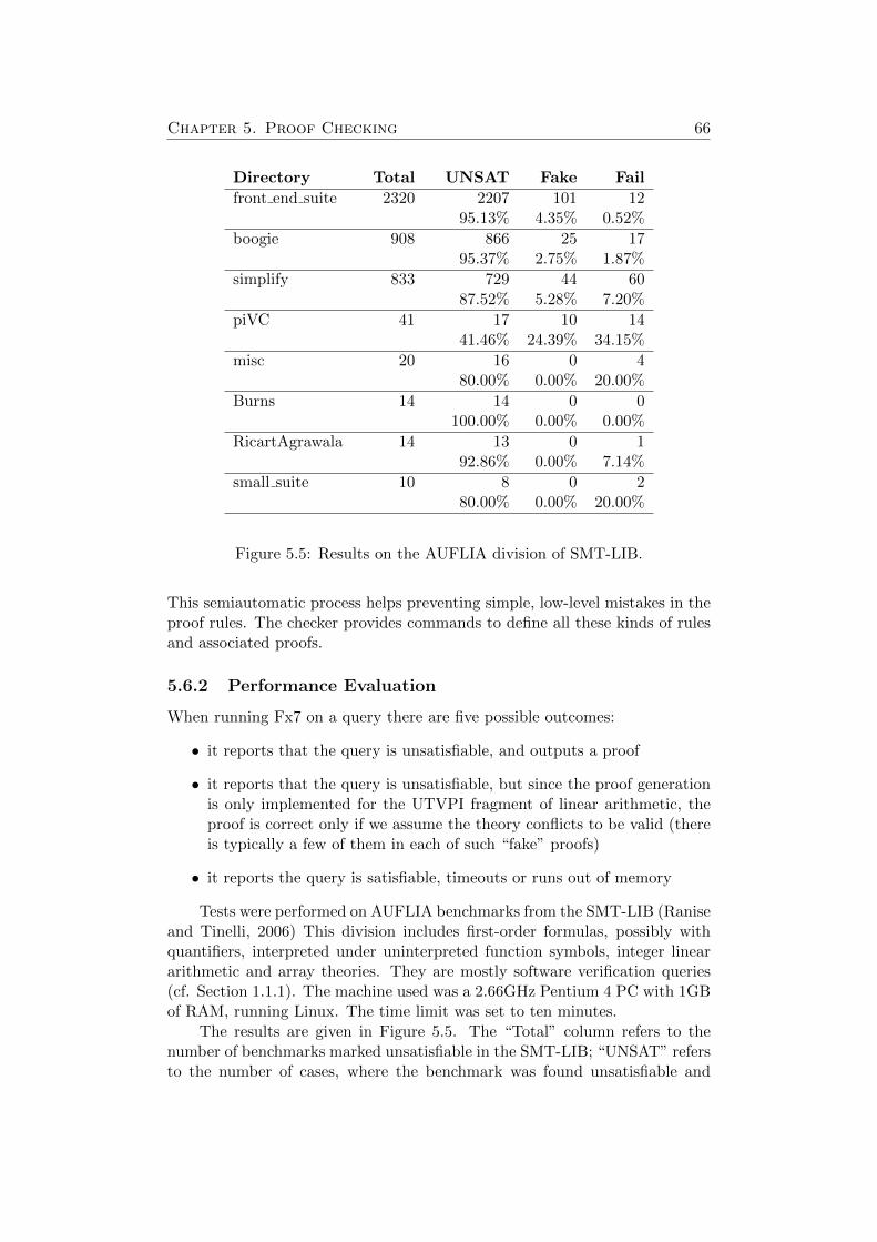
Chapter 5. Proof Checking 66
Directory Total UNSAT Fake Fail
front end suite 2320 2207 101 1295.13% 4.35% 0.52%
boogie 908 866 25 1795.37% 2.75% 1.87%
simplify 833 729 44 6087.52% 5.28% 7.20%
piVC 41 17 10 1441.46% 24.39% 34.15%
misc 20 16 0 480.00% 0.00% 20.00%
Burns 14 14 0 0100.00% 0.00% 0.00%
RicartAgrawala 14 13 0 192.86% 0.00% 7.14%
small suite 10 8 0 280.00% 0.00% 20.00%
Figure 5.5: Results on the AUFLIA division of SMT-LIB.
This semiautomatic process helps preventing simple, low-level mistakes in theproof rules. The checker provides commands to define all these kinds of rulesand associated proofs.
5.6.2 Performance Evaluation
When running Fx7 on a query there are five possible outcomes:
• it reports that the query is unsatisfiable, and outputs a proof
• it reports that the query is unsatisfiable, but since the proof generationis only implemented for the UTVPI fragment of linear arithmetic, theproof is correct only if we assume the theory conflicts to be valid (thereis typically a few of them in each of such “fake” proofs)
• it reports the query is satisfiable, timeouts or runs out of memory
Tests were performed on AUFLIA benchmarks from the SMT-LIB (Raniseand Tinelli, 2006) This division includes first-order formulas, possibly withquantifiers, interpreted under uninterpreted function symbols, integer lineararithmetic and array theories. They are mostly software verification queries(cf. Section 1.1.1). The machine used was a 2.66GHz Pentium 4 PC with 1GBof RAM, running Linux. The time limit was set to ten minutes.
The results are given in Figure 5.5. The “Total” column refers to thenumber of benchmarks marked unsatisfiable in the SMT-LIB; “UNSAT” refersto the number of cases, where the benchmark was found unsatisfiable and

Chapter 5. Proof Checking 67
a correct proof was generated; “Fake” is the number of benchmarks foundunsatisfiable, but with “fake” proofs; finally “Fail” is the number of cases,where Fx7 was unable to prove it within the time limit. It should be the casethat UNSAT + Fake + Fail = Total. The percentages are with respect to theTotal.
With the C implementation, proof checking a single proof never tookmore than 7 seconds. It took more than 2 seconds in 4 cases and more than1 second in 19 cases (therefore the average time is well under a second). Themaximal amount of memory consumed for a single proof was never over 7MB,with average being 2MB.
We have also tested the C implementation on a Dell x50v PDA with a624MHz XScale ARM CPU and 32MB of RAM, running Windows CE. It wasabout 6 times slower than the Pentium machine, but was otherwise perfectlycapable of running the checker. This fact can be thought of as a first step on away to PCC-like scenarios on small, mobile devices. Other devices of similarcomputing power and, what is more important, RAM amount include mostsmart phones and iPods.
The OCaml implementation was on average 3 times slower than theC version, it also tends to consume more memory, mostly because it keepsall the terms forever (which is because of our implementation, not because ofOCaml).
We have also experimented with translating the proof objects into theMaude syntax (Clavel et al., 2001). We have implemented lambda terms andbeta reduction using the built-in Maude integers to encode de Bruijn indicesand used the standard equational specifications for the first-order rules. Theresulting Maude implementation is very compact (about 60 lines), but theperformance is not as good as with the OCaml or C implementation — itis between 10 and 100 times slower than the OCaml one. It also tends toconsume a lot more memory. The reason is mainly the non-native handling oflambda expressions. Beta reductions translate to large number of first-orderrewrites, which are then memoized, and we were unable to instrument Maudeto skip memoization of those.
We have performed some experiments using Coq metalogic as the proofchecker. We did not get as far as implementing our own object logic. The mainobstacle we have found was the treatment of binders. Performing skolemiza-tion on a typical input results in hundreds of Skolem functions. When usinga higher order logic prover, such functions are existentially quantified and thequantifiers need to be pushed through the entire formula to the beginning.Later, during the proof, we need to go through them to manipulate the for-mula. This puts too much pressure on the algorithms treating of binders in thehigher order prover. In our approach Skolem functions are bound implicitly,so there is no need to move them around. This is especially important in SMTqueries, where the vast majority of the input formula is ground and quantifiedsubformulas occur only deep inside the input. We can therefore keep most ofthe formula binder-free. We were not able to perform any realistic tests, as

Chapter 5. Proof Checking 68
Coq was running out of memory.
Both Maude and Coq are far more general purpose tools than just proofcheckers. However relatively good results with Maude suggest that using asimple underlying formalism is beneficial in proof checking scenarios.
5.7 Related and Future Work
CVC3 (Barrett and Tinelli, 2007) and Fx7 were the only solvers participatingin the 2007 edition of the SMT competition to produce formal proofs. Theproof generation in CVC3 is based on the LF framework. We are not awareof a published work evaluating proof checking techniques on large industrialbenchmarks involving quantifiers.
Formalisms for checking SMT proofs have been proposed in the past,most notably using an optimized implementation (Stump and Dill, 2002)of Edinburgh Logical Framework (Harper et al., 1987). However even withthe proposed optimizations, the implementations has an order of magnitudehigher memory requirements than our solution. Also the implementation ofthe checker is much more complicated.
Recently a Signature Compiler tool has been proposed (Zeller et al., 2008).It generates a custom proof checker in C++ or Java from a LF signature. Wehave run our proof checker on a 1:1 translation of the artificial EQ benchmarksfrom the paper. It is running slightly faster than the generated C++ checker.The memory requirements of our implementation are way below the size ofthe input file on those benchmarks. The checkers remain to be compared onreal benchmarks involving richer logics and quantifiers.
In the context of saturation theorem provers it is very natural to outputthe proof just as a sequence of resolution or superposition steps. What ismissing here, is the proof of CNF translation, though proof systems has beenproposed (de Nivelle, 2005, 2003) to deal with that.
Finally, work on integrating SMT solvers as decision procedures insidehigher order logic provers include (McLaughlin et al., 2006; Fontaine et al.,2006), (Conchon et al., 2007). The main problem with these approaches isthat proof generation is usually at least order of magnitude faster than proofchecking inside higher order logic prover. The Ergo (Conchon et al., 2007)paper mentions promising preliminary results with using proof traces insteadof full proofs with Coq for theory conflicts. It is possible that using tracescould also work for CNF conversion and skolemization. Yet another approachmentioned there is verifying the SMT solver itself.
An important remaining problem is the treatment of theory conflicts. Onescenario here is to extend the linear arithmetic decision procedure to produceproofs. It should be possible to encode the proofs with just a minor extensionsto the rewrite formalism. Another feasible scenario is to use a different SMTsolver as a oracle for checking the harder (or all) theory conflicts. This can beapplied also to other theories, like bit vectors or rational arithmetic.

Chapter 5. Proof Checking 69
5.8 Conclusions
We have shown how term rewriting can be used for proof checking. Thehighlights of our approach are:
1. time and space efficiency of the proof checker
2. simplicity of the formalism, and thus simplicity of the implementation
3. semiautomatic checking of proof rules
The main technical insight is that the proof rules can be executed locally.Therefore the memory taken by proofs trees can be reclaimed just after check-ing them and reused for the subsequent fragments of the proof tree.

Chapter 5. Proof Checking 70

Chapter 6
Conclusions and FutureResearch
This thesis tackled several issues concerning interconnection between softwareverification tools and SMT solvers. After introduction and setting up thecontext, Chapter 3 gave a survey of methods for programming a verificationbackground theory in an SMT solver, using triggering annotations. Chapter 4gave algorithms to be employed in an SMT solver, so it can respond promptlyto such programming. Finally, Chapter 5 talked about correctness assuranceof such responses.
The particular area of interest was verification it its full glory: sound,formal, concerned with high-level, functional properties. This is where theaxiomatization techniques of Chapter 3 are most useful, and this is also wherethe PCC scenarios enabled by techniques of Chapter 5 allow for maximal trustimprovement. The grand question, however, is whether it makes sense at all.Is it advisable to use SMT solvers for full-blown verification of functional prop-erties of software? Or should we just stay with interactive theorem provingor, worse yet, informal correctness arguments, augmented by testing?
The experience with VCC, in the Hypervisor verification and otherwise,suggests that SMT is surprisingly powerful, when it comes to functional veri-fication. This is supported by successful verification of several highly concur-rent, but also significant in implementation size, algorithms in the Hypervi-sor. A small, self contained example is a reader-writer lock, verified inside thesystem with very natural external specifications (Hillebrand and Leinenbach,2009).
Unfortunately, it is also very brittle, both in expressive capabilities andperformance. While Chapter 3 lists several tools and methods for solving someof those problems, it would definitely be beneficial to work with a more pre-dictable technology, and thus more research is needed on effective approachesto programming verification theories in SMT solvers. Still, SMT seems like apreferable choice, compared to interactive theorem proving, for main-streamverification.
When it comes to the theory programming, the triggering annotations
71

Chapter 6. Conclusions and Future Research 72
have much in common with term rewriting. Chapter 5 have demonstratedhow first-order rewriting combined with lambda abstractions can be used toprogram a logic for a proof checker. The lambda abstractions, while theoreti-cally very powerful, were easy to implement efficiently, giving rise to fast andlean proof checker. Possibly a similar approach could be used in the SMTsolver instead, for programming verification theories.

Bibliography
(Babic and Hutter, 2008) Domagoj Babic and Frank Hutter. Spear theorem prover.In Proc. of the SAT 2008 Race, 2008.
(Ball et al., 2005) Thomas Ball, Shuvendu K. Lahiri, and Madanlal Musuvathi.Zap: Automated theorem proving for software analysis. In Geoff Sutcliffeand Andrei Voronkov, editors, LPAR, volume 3835 of Lecture Notes in Com-puter Science, pages 2–22. Springer, 2005. ISBN 3-540-30553-X.
(Barnett et al., 2005) Mike Barnett, K. Rustan M. Leino, and Wolfram Schulte.The Spec# programming system: An overview. In Gilles Barthe, LilianBurdy, Marieke Huisman, Jean-Louis Lanet, and Traian Muntean, editors,Construction and Analysis of Safe, Secure, and Interoperable Smart devices(CASSIS 2004), volume 3362 of Lecture Notes in Computer Science, pages49–69. Springer-Verlag, 2005. URL http://www.springerlink.com/content/0m789xre652nuv06.
(Barnett et al., 2006) Mike Barnett, Bor-Yuh Evan Chang, Robert DeLine, BartJacobs, and K. Rustan M. Leino. Boogie: A modular reusable verifier forobject-oriented programs. In Frank S. de Boer, Marcello M. Bonsangue,Susanne Graf, and Willem-Paul de Roever, editors, Formal Methods forComponents and Objects: 4th International Symposium, FMCO 2005, vol-ume 4111 of Lecture Notes in Computer Science, pages 364–387. Springer,September 2006.
(Barrett and Berezin, 2004) Clark Barrett and Sergey Berezin. CVC Lite: A newimplementation of the Cooperating Validity Checker. In Rajeev Alur andDoron A. Peled, editors, Proceedings of the 16th International Conferenceon Computer Aided Verification (CAV ’04), volume 3114 of Lecture Notesin Computer Science, pages 515–518. Springer-Verlag, July 2004.
(Barrett and Tinelli, 2007) Clark Barrett and Cesare Tinelli. CVC3. In WernerDamm and Holger Hermanns, editors, CAV, volume 4590 of LNCS, pages298–302. Springer, 2007. ISBN 978-3-540-73367-6.
(Barrett et al., 1996) Clark Barrett, David Dill, and Jeremy Levitt. Validity check-ing for combinations of theories with equality. In Mandayam Srivas and Al-bert Camilleri, editors, Formal Methods In Computer-Aided Design, volume
73

BIBLIOGRAPHY 74
1166 of Lecture Notes in Computer Science, pages 187–201. Springer-Verlag,November 1996. Palo Alto, California, November 6–8.
(Barrett et al., 2008) Clark Barrett, Morgan Deters, Albert Oliveras, and AaronStump. Design and results of the 3rd annual satisfiability modulo theoriescompetition (smt-comp 2007). International Journal on Artificial Intelli-gence Tools, 17(4):569–606, 2008.
(Barthe et al., 2006) Gilles Barthe, Lilian Burdy, Julien Charles, BenjaminGregoire, Marieke Huisman, Jean-Louis Lanet, Mariela Pavlova, and An-toine Requet. Jack - a tool for validation of security and behaviour of javaapplications. In Frank S. de Boer, Marcello M. Bonsangue, Susanne Graf,and Willem P. de Roever, editors, FMCO, volume 4709 of Lecture Notes inComputer Science, pages 152–174. Springer, 2006. ISBN 978-3-540-74791-8.
(Baumann et al., 2009) Christoph Baumann, Bernhard Beckert, Holger Blasum,and Thorsten Bormer. Better avionics software reliability by code verifica-tion – A glance at code verification methodology in the Verisoft XT project.In Embedded World 2009 Conference, Nuremberg, Germany, March 2009.Franzis Verlag. URL http://www.uni-koblenz.de/˜beckert/pub/embeddedworld2009.pdf. To appear.
(Bohme et al., 2009) Sascha Bohme, Micha l Moskal, Wolfram Schulte, andBurkhart Wolff. HOL-Boogie: An interactive prover-backend for the Veri-fiying C Compiler. Journal of Automated Reasoning, 2009. To appear.
(Bozzano et al., 2005) Marco Bozzano, Roberto Bruttomesso, Alessandro Cimatti,Tommi Junttila, Peter Rossum, Stephan Schulz, and Roberto Sebastiani.MathSAT: Tight integration of SAT and mathematical decision procedures.J. Autom. Reason., 35(1-3):265–293, 2005. ISSN 0168-7433. doi: http://dx.doi.org/10.1007/s10817-005-9004-z.
(Bryant et al., 2002) Randal E. Bryant, Shuvendu K. Lahiri, and Sanjit A. Seshia.Modeling and verifying systems using a logic of counter arithmetic withlambda expressions and uninterpreted functions. In CAV ’02: Proceedingsof the 14th International Conference on Computer Aided Verification, pages78–92, London, UK, 2002. Springer-Verlag. ISBN 3-540-43997-8.
(Clavel et al., 2001) Manuel Clavel, Francisco Duran, Steven Eker, Patrick Lincoln,Narciso Martı-Oliet, Jose Meseguer, and Jose F. Quesada. Maude: Specifi-cation and programming in rewriting logic. Theoretical Computer Science,2001.
(Cohen et al., 2009a) Ernie Cohen, Markus Dahlweid, Mark Hillebrand, DirkLeinenbach, Micha l Moskal, Thomas Santen, Wolfram Schulte, and StephanTobies. VCC: A practical system for verifying concurrent C. In StefanBerghofer, Tobias Nipkow, Christian Urban, and Markus Wenzel, editors,Theorem Proving in Higher Order Logics (TPHOLs 2009), volume 5674 of

BIBLIOGRAPHY 75
Lecture Notes in Computer Science, pages 23–42, Munich, Germany, 2009a.Springer. Invited paper.
(Cohen et al., 2009b) Ernie Cohen, Micha l Moskal, Wolfram Schulte, and StephanTobies. A practical verification methodology for concurrent programs. Tech-nical Report MSR-TR-2009-15, Microsoft Research, February 2009b. Avail-able from http://research.microsoft.com/pubs.
(Cohen et al., 2009c) Ernie Cohen, Micha l Moskal, Wolfram Schulte, and StephanTobies. A Precise Yet Efficient Memory Model For C. In Proceedings ofSystems Software Verification Workshop (SSV 2009), 2009c. To appear.
(Conchon et al., 2007) Sylvain Conchon, Evelyne Contejean, Johannes Kanig, andStephane Lescuyer. Lightweight integration of the Ergo theorem proverinside a proof assistant. In Second Automated Formal Methods workshopseries (AFM07), Atlanta, Georgia, USA, November 2007.
(Darvas and Leino, 2007) Adam Darvas and K. Rustan M. Leino. Practical reason-ing about invocations and implementations of pure methods. In Matthew B.Dwyer and Antonia Lopes, editors, FASE, volume 4422 of Lecture Notes inComputer Science, pages 336–351. Springer, 2007. ISBN 978-3-540-71288-6.
(Davis and Putnam, 1960) Martin Davis and Hilary Putnam. A computing proce-dure for quantification theory. J. ACM, 7(3):201–215, 1960.
(Davis et al., 1962) Martin Davis, George Logemann, and Donald W. Loveland. Amachine program for theorem-proving. Commun. ACM, 5(7):394–397, 1962.
(de Bruijn, 1972) N.G. de Bruijn. Lambda-calculus notation with nameless dum-mies: a tool for automatic formula manipulation with application to theChurch-Rosser theorem. Indag. Math., 34(5):381–392, 1972.
(de Moura and Bjørner, 2008) Leonardo de Moura and Nikolaj Bjørner. Z3: AnEfficient SMT Solver, volume 4963/2008 of Lecture Notes in Computer Sci-ence, pages 337–340. Springer Berlin, April 2008.
(de Nivelle, 2003) Hans de Nivelle. Implementing the clausal normal form transfor-mation with proof generation. In fourth workshop on the implementationof logics, pages 69–83, Almaty, Kazachstan, 2003. University of Liverpool,University of Manchester.
(de Nivelle, 2005) Hans de Nivelle. Translation of resolution proofs into short first-order proofs without choice axioms. Information and Computation, 199(1):24–54, April 2005.
(DeLine and Leino, 2005) Robert DeLine and K. Rustan M. Leino. BoogiePL: Atyped procedural language for checking object-oriented programs. TechnicalReport MSR-TR-2005-70, Microsoft Research, March 2005.

BIBLIOGRAPHY 76
(Detlefs et al., 2005) David Detlefs, Greg Nelson, and James B. Saxe. Simplify: atheorem prover for program checking. Journal of the ACM, 52(3):365–473,May 2005.
(Detlefs et al., 1998) David L. Detlefs, K. Rustan M. Leino, Greg Nelson, andJames B. Saxe. Extended static checking. SRC Research Report 159, Com-paq Systems Research Center, 130 Lytton Ave., Palo Alto, December 1998.
(Dijkstra, 1972) E. W. Dijkstra. The humble programmer. Communications of theACM, 15(10):859–886, October 1972. Reprinted in Programming Methodol-ogy, A Collection of Articles by Members of IFIP WG2.3 , D. Gries (ed.),Springer-Verlag, 1978.
(Dutertre and de Moura, 2006) Bruno Dutertre and Leonardo Mendonca de Moura.A fast linear-arithmetic solver for DPLL(T). In Thomas Ball and Robert B.Jones, editors, CAV, volume 4144 of LNCS, pages 81–94. Springer, 2006.ISBN 3-540-37406-X.
(Een and Sorensson, 2003) Niklas Een and Niklas Sorensson. An extensible SAT-solver. In Enrico Giunchiglia and Armando Tacchella, editors, SAT, volume2919 of Lecture Notes in Computer Science, pages 502–518. Springer, 2003.ISBN 3-540-20851-8.
(Filliatre, 2003) Jean-Christophe Filliatre. Why: a multi-language multi-prover ver-ification tool. Research Report 1366, LRI, Universite Paris Sud, March 2003.
(Flanagan et al., 2002) Cormac Flanagan, K. Rustan M. Leino, Mark Lillibridge,Greg Nelson, James B. Saxe, and Raymie Stata. Extended static check-ing for Java. In Proceedings of the 2002 ACM SIGPLAN Conference onProgramming Language Design and Implementation (PLDI), volume 37 ofSIGPLAN Notices, pages 234–245. ACM, May 2002.
(Flanagan et al., 2004) Cormac Flanagan, Rajeev Joshi, and James B. Saxe. Anexplicating theorem prover for quantified formulas. Technical Report 199,HP Labs, 2004.
(Fontaine et al., 2006) Pascal Fontaine, Jean-Yves Marion, Stephan Merz, LeonorPrensa Nieto, and Alwen Tiu. Expressiveness + automation + soundness:Towards combining SMT solvers and interactive proof assistants. In Hol-ger Hermanns and Jens Palsberg, editors, Tools and Algorithms for theConstruction and Analysis of Systems (TACAS’06), volume 3920 of LNCS,pages 167–181. Springer-Verlag, 2006.
(Ganzinger et al., 2004) H. Ganzinger, G. Hagen, R. Nieuwenhuis, A. Oliveras, andC. Tinelli. DPLL(T): Fast Decision Procedures. In R. Alur and D. Peled,editors, 16th International Conference on Computer Aided Verification,CAV’04, volume 3114 of Lecture Notes in Computer Science, pages 175–188. Springer, 2004.

BIBLIOGRAPHY 77
(Ge et al., 2007) Yeting Ge, Clark Barrett, and Cesare Tinelli. Solving quantifiedverification conditions using satisfiability modulo theories. In Frank Pfen-ning, editor, CADE, volume 4603 of LNCS, pages 167–182. Springer, 2007.ISBN 978-3-540-73594-6.
(Harper et al., 1987) Robert Harper, Furio Honsell, and Gordon Plotkin. A frame-work for defining logics. In Proceedings 2nd Annual IEEE Symp. onLogic in Computer Science, LICS’87, Ithaca, NY, USA, 22–25 June 1987,pages 194–204. IEEE Computer Society Press, New York, 1987. URLciteseer.ist.psu.edu/harper87framework.html.
(Harvey and Stuckey, 1997) W. Harvey and P. Stuckey. A unit two variable perinequality integer constraint solver for constraint logic programming, 1997.URL citeseer.ist.psu.edu/harvey97unit.html.
(Hillebrand and Leinenbach, 2009) Mark A. Hillebrand and Dirk C. Leinenbach.Formal verification of a reader-writer lock implementation in C. In 4th In-ternational Workshop on Systems Software Verification (SSV 2009), Elec-tronic Notes in Theoretical Computer Science. Elsevier Science B.V., 2009.To appear.
(Janota et al., 2007) Mikolas Janota, Radu Grigore, and Micha l Moskal.Reachability analysis for annotated code. In Sixth InternationalWorkshop on Specification and Verification of Component-Based Sys-tems (SAVCBS 2007), pages 23–30. ACM, September 2007. URLhttp://www.cs.iastate.edu/˜leavens/SAVCBS/2007/papers/Janota-Grigore-Moskal.pdf.
(Kiniry and Cok, 2005) Joseph R. Kiniry and David R. Cok. ESC/Java2: UnitingESC/Java and JML: Progress and issues in building and using ESC/Java2and a report on a case study involving the use of ESC/Java2 to verifyportions of an Internet voting tally system. In Construction and Analysisof Safe, Secure and Interoperable Smart Devices: International Workshop,CASSIS 2004, volume 3362 of LNCS, 2005.
(Kozen, 1977) Dexter Kozen. Complexity of finitely generated algebras. In Pro-ceedings of the 9th Symposium on Theory of Computing, pages 164–177,1977.
(Lahiri and Qadeer, 2008) Shuvendu K. Lahiri and Shaz Qadeer. Back to the fu-ture: revisiting precise program verification using SMT solvers. In George C.Necula and Philip Wadler, editors, POPL, pages 171–182. ACM, 2008. ISBN978-1-59593-689-9.
(Leavens et al., 1999) Gary T. Leavens, Albert L. Baker, and Clyde Ruby. JML:A notation for detailed design. In Haim Kilov, Bernhard Rumpe, and IanSimmonds, editors, Behavioral Specifications of Businesses and Systems,pages 175–188. Kluwer Academic Publishers, Boston, 1999.

BIBLIOGRAPHY 78
(Leino, 2009) K. Rustan M. Leino. This is Boogie 2, 2009. http://research.microsoft.com/˜leino/papers/krml178.pdf.
(Leino and Monahan, 2009) K. Rustan M. Leino and Rosemary Monahan. Reason-ing about comprehensions with first-order SMT solvers. In Sung Y. Shinand Sascha Ossowski, editors, SAC, pages 615–622. ACM, 2009. ISBN 978-1-60558-166-8.
(Leino et al., 2005) K. Rustan M. Leino, Todd Millstein, and James B. Saxe. Gener-ating error traces from verification-condition counterexamples. Sci. Comput.Program., 55(1-3):209–226, 2005. ISSN 0167-6423.
(Luckham et al., 1979) David C. Luckham, Steven M. German, Friedrich W. vonHenke, Richard A. Karp, P. W. Milne, Derek C. Oppen, Wolfgang Polak,and William L. Scherlis. Stanford Pascal Verifier user manual. Technical Re-port CS-TR-79-731, Stanford University, Department of Computer Science,March 1979.
(Malik et al., 2001) Sharad Malik, Ying Zhao, Conor F. Madigan, Lintao Zhang,and Matthew W. Moskewicz. Chaff: Engineering an efficient satsolver. Design Automation Conference, 0:530–535, 2001. doi: http://doi.ieeecomputersociety.org/10.1109/DAC.2001.935565.
(Marche et al., 2004) Claude Marche, Christine Paulin-Mohring, and Xavier Ur-bain. The krakatoa tool for certificationof java/javacard programs annotatedin jml. J. Log. Algebr. Program., 58(1-2):89–106, 2004.
(McLaughlin et al., 2006) Sean McLaughlin, Clark Barrett, and Yeting Ge. Co-operating theorem provers: A case study combining HOL-Light and CVCLite. In Alessandro Armando and Alessandro Cimatti, editors, Proceedingsof the 3rd Workshop on Pragmatics of Decision Procedures in AutomatedReasoning (PDPAR ’05), volume 144(2) of Electronic Notes in TheoreticalComputer Science, pages 43–51. Elsevier, January 2006. Edinburgh, Scot-land.
(Moskal, 2007) Micha l Moskal. Fx7 or it is all about quantifiers, 2007. Also,http://nemerle.org/fx7/.
(Moskal et al., 2007) Micha l Moskal, Kamil Skalski, Pawe l Olszta, et al. Nemerleprogramming language, 2007. http://nemerle.org/.
(Moy, 2009) Yannick Moy. Automatic Modular Static Safety Checking for C Pro-grams. PhD thesis, Universite Paris-Sud, January 2009.
(Necula, 1997) George C. Necula. Proof-carrying code. In ConferenceRecord of POPL ’97: The 24th ACM SIGPLAN-SIGACT Sym-posium on Principles of Programming Languages, pages 106–119,Paris, France, jan 1997. URL citeseer.ist.psu.edu/article/necula97proofcarrying.html.

BIBLIOGRAPHY 79
(Nelson and Oppen, 1979) Greg Nelson and Derek C. Oppen. Simplification bycooperating decision procedures. ACM Transactions on Programming Lan-guages and Systems, 1(2):245–257, October 1979.
(Nieuwenhuis and Oliveras, 2005) R. Nieuwenhuis and A. Oliveras. Proof-Producing Congruence Closure. In J. Giesl, editor, 16th International Con-ference on Term Rewriting and Applications, RTA’05, volume 3467 of Lec-ture Notes in Computer Science, pages 453–468. Springer, 2005.
(Owre et al., 1992) S. Owre, J. M. Rushby, and N. Shankar. PVS: A prototypeverification system. In Deepak Kapur, editor, 11th International Conferenceon Automated Deduction (CADE), volume 607 of Lecture Notes in ArtificialIntelligence, pages 748–752, Saratoga, NY, jun 1992. Springer-Verlag. URLhttp://www.csl.sri.com/papers/cade92-pvs/.
(Plotkin, 1972) Gordon D. Plotkin. Building-in equational theories. In D. Michieand B. Meltzer, editors, Machine Intelligence, pages 73–90. Edinburgh Uni-versity Press, 1972.
(Ramakrishnan et al., 2001) I. V. Ramakrishnan, R. C. Sekar, and AndreiVoronkov. Term indexing. In John Alan Robinson and Andrei Voronkov,editors, Handbook of Automated Reasoning, pages 1853–1964. Elsevier andMIT Press, 2001. ISBN 0-444-50813-9, 0-262-18223-8.
(Ranise and Tinelli, 2006) Silvio Ranise and Cesare Tinelli. The SMT-LIB Stan-dard: Version 1.2. Technical report, Department of Computer Science, TheUniversity of Iowa, 2006. Available at www.SMT-LIB.org.
(Saxe and Leino, 1999) Jim Saxe and K. Rustan M. Leino. ESC/Javadesign note 8a: The logic of ESC/Java, 1999. Available athttp://secure.ucd.ie/products/opensource/ESCJava2/ESCTools/docs/design-notes/escj08a.html.
(Stump and Dill, 2002) A. Stump and D. Dill. Faster Proof Checking in the Edin-burgh Logical Framework. In 18th International Conference on AutomatedDeduction, 2002.
(Stump et al., 2002) Aaron Stump, Clark W. Barrett, and David L. Dill. CVC: Acooperating validity checker. In Ed Brinksma and Kim Guldstrand Larsen,editors, Proceedings of the 14th International Conference on Computer AidedVerification (CAV ’02), volume 2404 of Lecture Notes in Computer Science,pages 500–504. Springer-Verlag, July 2002. Copenhagen, Denmark.
(Sutcliffe and Suttner, 1998) G. Sutcliffe and C.B. Suttner. The TPTP ProblemLibrary: CNF Release v1.2.1. Journal of Automated Reasoning, 21(2):177–203, 1998.
(Zeller et al., 2008) Michael Zeller, Aaron Stump, and Morgan Deters. Signaturecompilation for the Edinburgh Logical Framework. Electr. Notes Theor.Comput. Sci., 196:129–135, 2008.

![[3.5em]12th International Satisfiability Modulo Theories …smtcomp.sourceforge.net › 2017 › SMT-COMP-2017.pdf · 2017-09-05 · 12th International Satis ability Modulo Theories](https://img.dokumen.tips/doc/110x75/5f0ff8217e708231d446c9fe/35em12th-international-satisfiability-modulo-theories-a-2017-a-smt-comp-2017pdf.jpg)