Satellite constraint for emissions of nitrogen oxides from

Atmos. Chem. Phys., 12, 2881–2898, 2012www.atmos-chem-phys.net/12/2881/2012/doi:10.5194/acp-12-2881-2012© Author(s) 2012. CC Attribution 3.0 License.

AtmosphericChemistry

and Physics

Satellite constraint for emissions of nitrogen oxides fromanthropogenic, lightning and soil sources over East China on ahigh-resolution grid

J.-T. Lin

Laboratory for Climate and Ocean-Atmosphere Studies, Department of Atmospheric and Oceanic Sciences,School of Physics, Peking University, Beijing 100871, China

Correspondence to:J.-T. Lin ([email protected])

Received: 28 September 2011 – Published in Atmos. Chem. Phys. Discuss.: 7 November 2011Revised: 10 March 2012 – Accepted: 13 March 2012 – Published: 23 March 2012

Abstract. Vertical column densities (VCDs) of troposphericnitrogen dioxide (NO2) retrieved from space provide valu-able information to estimate emissions of nitrogen oxides(NOx) inversely. Accurate emission attribution to individ-ual sources, important both for understanding the global bio-geochemical cycling of nitrogen and for emission control,remains difficult. This study presents a regression-basedmulti-step inversion approach to estimate emissions of NOxfrom anthropogenic, lightning and soil sources individuallyfor 2006 over East China on a 0.25◦ long× 0.25◦ lat grid,employing the DOMINO product version 2 retrieved fromthe Ozone Monitoring Instrument. The inversion is donegridbox by gridbox to derive the respective emissions, tak-ing advantage of differences in seasonality between anthro-pogenic and natural sources. Lightning and soil emissionsare combined together for any given gridbox due to theirsimilar seasonality; and their different spatial distributionsare used implicitly for source separation to some extent. Thenested GEOS-Chem model for East Asia is used to simulatethe seasonal variations of different emission sources and im-pacts on VCDs of NO2 for the inversion purpose. Sensitivitytests are conducted to evaluate key assumptions embedded inthe inversion process. The inverse estimate suggests annualbudgets of about 7.1 TgN (±39 %), 0.21 TgN (±61 %), and0.38 TgN (±65 %) for the a posteriori anthropogenic, light-ning and soil emissions, respectively, about 18–23 % higherthan the respective a priori values. The enhancements in an-thropogenic emissions are largest in cities and areas with ex-tensive use of coal, particularly in the north in winter, as ev-ident on the high-resolution grid. Derived soil emissions areconsistent with recent bottom-up estimates. They are lessthan 6 % of anthropogenic emissions annually, increasing toabout 13 % for July. Derived lightning emissions are about3 % of anthropogenic emissions annually and about 10 % in

July. Overall, anthropogenic emissions are found to be thedominant source of NOx over East China with important im-plications for nitrogen control.

1 Introduction

Nitrogen oxides (NOx ≡ NO + NO2) are important con-stituents in the troposphere affecting the formation of ozoneand aerosols with significant consequences on air quality, cli-mate forcing and acid deposition. They are emitted from an-thropogenic combustion sources as well as natural sourcesfrom lightning, soil and biomass burning. Understanding theindividual contributions of anthropogenic and natural emis-sions is critical both for evaluating the effects of NOx onthe global environment and for forming appropriate emissioncontrol strategies in polluted areas like East China.

Satellite remote sensing provides data for vertical columndensities (VCDs) of nitrogen dioxide (NO2) in the tropo-sphere. The data can be used to estimate emissions of NOxfrom the top-down perspective supplementing the bottom-upestimate (e.g. Martin et al., 2003, 2006; Jaegle et al., 2005;Muller and Stavrakou, 2005; Richter et al., 2005; Wang etal., 2007; Zhang et al., 2007; Stavrakou et al., 2008; Zhaoand Wang, 2009; Lin et al., 2010a, b; Lin and McElroy,2010, 2011; Wang et al., 2012). Much attention has beenpaid to China due to its large and rapidly growing anthro-pogenic emissions (e.g. Richter et al., 2005; Martin et al.,2006; Wang et al., 2007; Zhang et al., 2007; Stavrakou etal., 2008; Zhao and Wang, 2009; Lin et al., 2010a, b; Linand McElroy, 2010, 2011; Wang et al., 2012). RetrievedVCDs, however, include contributions from all sources ofNOx, requiring additional information and assumptions indistinguishing individual sources.

Published by Copernicus Publications on behalf of the European Geosciences Union.

2882 J.-T. Lin: Space-based source attribution for nitrogen oxides

Several inversion studies have attempted to separate an-thropogenic from other sources of NOx, especially soilsources, based on measurements from the Global OzoneMonitoring Experiment (GOME) instrument (Jaegle etal., 2005; Muller and Stavrakou, 2005; Wang et al.,2007; Stavrakou et al., 2008), the Scanning ImagingAbsorption Spectrometer for Atmospheric CHartographY(SCIAMACHY) instrument (Muller and Stavrakou, 2005;Stavrakou et al., 2008), and the Ozone Monitoring Instru-ment (OMI) (Zhao and Wang, 2009). Jaegle et al. (2005)and Wang et al. (2007) proposed two different methods toseparate anthropogenic, soil and biomass burning emissionsmonth by month with no attempt to constrain lightning emis-sions. Jaegle et al. (2005) assumed the a posteriori non-lightning emissions to be solely anthropogenic if the a pri-ori anthropogenic emissions exceed 90 % of the a priori to-tal emissions or if they exceed the a posteriori non-lightningemissions. Otherwise, differences between the a posterioriand a priori emissions were attributed to soil or biomassburning sources. A similar criterion was adopted by Zhaoand Wang (2009) to differentiate anthropogenic and soilemissions. Wang et al. (2007) distinguished anthropogenicand soil sources using prescribed values for errors in the apriori anthropogenic emission data. Specifically, if the a pos-teriori non-lightning non-biomass burning emissions exceedthe a priori anthropogenic emissions plus errors (assumed tobe 40–60 %), the differences are attributed to soil sources.Muller and Stavrakou (2005) and Stavrakou et al. (2008)used an adjoint modeling approach for source attribution.Wang et al. (2007) suggested that soil emissions over EastChina amounted to 0.85 TgN per year for 1997–2000, differ-ing significantly from other inverse estimates (Jaegle et al.,2005; Muller and Stavrakou, 2005; Stavrakou et al., 2008;Zhao and Wang, 2009; L. Jaegle, personal communication,2011; C. Zhao and Y. Wang, personal communication, 2011).Soil emissions derived from the inverse modeling also dif-fer from the bottom-up estimates (Yienger and Levy, 1995;Yan et al., 2003, 2005; Hudman et al., 2012; Steinkamp andLawrence, 2011); in particular, they are 50–300 % larger thanthe Yienger and Levy (1995) estimate. According to Jaegleet al. (2005) and Wang et al. (2007), soil emissions may beas large as 40–50 % of anthropogenic emissions in summerfor East Asia in 2000 and for East China in 1997–2000, re-spectively, with significant implications for the global bio-geochemical cycling of nitrogen.

The magnitude of lightning emissions is difficult to es-timate (Boersma et al., 2005; Schumann and Huntrieser,2007), especially on the regional scale with significant vari-ations in lightning occurrences from one year to another(Schumann and Huntrieser, 2007). Most inverse estimatesdid not attempt to constrain lightning emissions (Jaegle etal., 2005; Wang et al., 2007; Zhao and Wang, 2009; Lin etal., 2010a, b; Lin and McElroy, 2010). The inverse model-ing by Stavrakou et al. (2008) suggested lightning emissionsto be 50–80 % larger than their a priori values (3 TgN yr−1

globally) with the largest difference over the tropics; thestudy did not specify the magnitude of lightning emissionsover China.

This study presents a new method to inversely deriveemissions of NOx for 2006 over East China (101.25◦ E–126.25◦ E, 19◦–46◦ N; see Fig. 1) from anthropogenic, light-ning and soil sources individually based on satellite re-trievals of NO2 columns and simulations of the global chem-ical transport model (CTM) GEOS-Chem. Emissions frombiomass burning are not constrained since they are unimpor-tant over East China (Wang et al., 2007; Lin et al., 2010a).A regression-based multi-step inversion approach is used toderive emissions for all months, exploiting information onthe seasonal variations of individual sources simulated by theCTM. The satellite data are taken from the DOMINO productversion 2 (DOMINO-2) retrieved by the Royal NetherlandsMeteorological Institute (KNMI) from the Ozone Monitor-ing Instrument (OMI) (Boersma et al., 2007, 2011). Thenested GEOS-Chem model for East Asia (Chen et al., 2009)is used to calculate VCDs of NO2 in response to vari-ous emission sources for the inversion purpose. The top-down emissions are derived at a relatively fine resolution of0.25◦ long× 0.25◦ lat allowing for a more detailed analysisof the spatial distribution of emissions, compared to previ-ous studies (Jaegle et al., 2005; Muller and Stavrakou, 2005;Wang et al., 2007; Stavrakou et al., 2008; Zhao and Wang,2009).

The paper is organized as follows. Section 2 presents thesatellite product. Section 3 describes the CTM and com-pares simulated VCDs with retrieved values. Section 4 de-scribes the inversion process in detail and analyzes the re-sulting top-down emissions for anthropogenic, lightning andsoil sources. It also evaluates the effects of key assumptionsmade during the inversion process. Section 5 presents thea posteriori emissions in comparison with previous inverseand bottom-up estimates. Section 6 concludes the presentanalysis.

2 VCDs of NO2 retrieved from OMI

The KNMI DOMINO-2 product offers a level-2 dataset forVCDs of NO2 derived by three main steps involving thecalculation of slant column densities (SCDs), troposphericSCDs, and tropospheric VCDs (Boersma et al., 2007, 2011).The derivation relies on information on air mass factors(AMFs) to convert the tropospheric SCDs to VCDs. TheAMFs are interpolated from a look-up table (LUT), and aresubject to errors in the predetermined information for clouds,aerosols, surface albedo, the a priori vertical profile of NO2,surface pressure, and surface height. The reader is referredto Boersma et al. (2007, 2011) for detailed derivation of theproduct.

Errors in retrieved VCDs are derived mainly from the cal-culation of SCDs and its tropospheric portion over cleaner

Atmos. Chem. Phys., 12, 2881–2898, 2012 www.atmos-chem-phys.net/12/2881/2012/

J.-T. Lin: Space-based source attribution for nitrogen oxides 2883

35

1

Figure 1. 2

3

4

5

6

7

8

9

10

11

12

13

14

Fig. 1. Regional specifications with provincial boundaries for EastChina. Also presented are its subregions, provinces and province-level municipalities discussed in the text: the Yangtze River Delta(YRD), the Pearl River Delta (PRD), the Sichuan Basin, the Bo-hai Sea, Beijing (BJ), Shanghai, Hebei, Henan, Shandong, Shanxi,Ningxia, Inner-Mongolia, and Sichuan. On the background is theannual mean VCDs of NO2 from the DOMINO-2 product.

regions, and are mainly from the calculation of AMFs forpolluted regions (Boersma et al., 2007). Compared to ver-sion 1, DOMINO-2 incorporates a variety of improvementson the LUT, surface albedo, and the a priori vertical pro-file of NO2 (Boersma et al., 2011). It also includes a cross-track stripe correction and a high-resolution dataset for sur-face height. As a result, systematic biases found in ver-sion 1 are reduced significantly in DOMINO-2 (Boersmaet al., 2011). The overall error for retrieved VCDs inDOMINO-2 is estimated to be about 30 % (a relative error)plus 0.7× 1015 molec. cm−2 (an absolute error), likely witha magnitude larger in winter than in summer (Boersma et al.,2007, 2011; Lin and McElroy, 2010, 2011; Lin et al., 2010a).In this study, the relative error is assumed to vary nonlinearlyfrom 30 % in summer to 50 % in winter based on the follow-ing formula: 0.3 + 0.2× (1− sin(i/10×π)), wherei = 0, 1,2, 3, 4, 5, 5, 4, 3, 2, 1, 0 for months from January to De-cember. This information will be employed for purposes ofemission inversion; and the assumed seasonality will be eval-uated in Sect. 4.6.

In this study, the daily level-2 data from DOMINO-2 aregridded to 0.25◦ long× 0.25◦ lat, which are averaged thento obtain monthly mean VCDs for subsequent emission in-version. The level-2 dataset includes measurements at 60viewing angles corresponding to 60 ground pixels, and thepixel sizes increase nonlinearly from 13× 24 km2 at nadir

to 25× ∼140 km2 at the edges of the viewing swath. Thisstudy excludes pixels with cloud radiance fraction exceeding50 % (Boersma et al., 2007). In addition, it only uses datafrom the 30 pixels around the swath center (with a cross-track length less than 30 km), allowing for a better analysisof the spatial distribution of VCDs within short distances.It consequently changes the swath width in use to about800 km so that global coverage is achieved roughly aboutevery three days. Note that the pixel sizes here are muchsmaller than the GOME (320× 40 km2) and SCIAMACHY(60× 30 km2) instruments used in previous inverse estimates(Jaegle et al., 2005; Muller and Stavrakou, 2005; Wang et al.,2007; Stavrakou et al., 2008).

3 Simulations of GEOS-Chem

3.1 Descriptions of model simulations

This study uses the nested model of GEOS-Chem(version 08-03-02;http://wiki.seas.harvard.edu/geos-chem/index.php/MainPage) for East Asia run at a horizontal resolu-tion of 0.667◦ long× 0.5◦ lat with 47 layers vertically (Chenet al., 2009). The model is run with the full Ox-NOx-CO-VOC-HOx chemistry. It is driven by the assimilated meteo-rological fields of GEOS-5 taken from the National Aero-nautics and Space Administration (NASA) Global Model-ing and Assimilation Office (GMAO). Vertical mixing in theplanetary boundary layer follows the non-local scheme (Linand McElroy, 2010) accounting for the varying magnitude ofmixing from stable to unstable states of the boundary layer.Convection is parameterized based on a modified versionof the Relaxed Arakawa-Schubert scheme by Moorthi andSuarez (1992) (Rienecker et al., 2008). The lateral boundaryconditions are updated every 3 h using results from associ-ated global simulations at 5◦ long× 4◦ lat horizontally.

Annual anthropogenic emissions of NOx, carbon monox-ide (CO) and non-methane volatile organic compounds(VOC) are taken from the INTEX-B dataset for 2006 pro-vided by Zhang et al. (2009), including sources from powerplants, industry, transportation and the residential sector.Emissions from the residential sector are further assumed tovary month to month accounting for heating related emis-sions that depend on ambient air temperature (Streets et al.,2003). They, however, contribute only 6 % of anthropogenicsources of NOx on the annual basis (Zhang et al., 2009).Emissions from power plants, industry and transportation areheld constant across the seasons since the seasonality is rel-atively small and is not included in the INTEX-B dataset.The impact of such simplification is found to be small (seeSect. 5). The diurnal variations of individual sources followLin et al. (2010a) and Lin and McElroy (2010, 2011).

Natural sources of NOx include lightning, soil andbiomass burning. Emissions from biomass burning are takenfrom the year-to-year varying monthly dataset of GFED2

www.atmos-chem-phys.net/12/2881/2012/ Atmos. Chem. Phys., 12, 2881–2898, 2012

http://wiki.seas.harvard.edu/geos-chem/index.php/Main Page

http://wiki.seas.harvard.edu/geos-chem/index.php/Main Page


(van der Werf et al., 2006); their magnitudes are negligiblefor NOx over China (Wang et al., 2007; Lin et al., 2010a) asthe relatively low combustion temperature does not allow forsignificant production of NOx. In 2006, the emission budgetfor East China is only about 0.013 TgN.

Production of NOx from lightning is determined by theflash rate multiplying the yield of nitric oxide (NO) fromeach flash. In GEOS-Chem, the NO yield is latitude de-pendent: over the Asian continent, the yield is set to be500 moles per flash north of 35◦ N reducing to 260 molesper flash south of 35◦ N (Martin et al., 2006; Hudman etal., 2007), based on previous observational constraint thatthe NO yield in the tropics is lower than in the midlatitude(Huntrieser et al., 2006). The total (intra-cloud and cloud-to-ground) flash rate is determined by convective cloud topheight to the 4.9th power over lands free of snow and ice,as formulated by Price et al. (1997). The total amount oflightning induced emissions is distributed vertically with abackward “C-shape” profile (Ott et al., 2010). Horizontally,as the flash rate depends on cloud properties that are highlyparameterized, it is subject to large uncertainties particularlyfor individual locations. Alternate lightning parameteriza-tions based on cloud mass flux or convective precipitation(Allen and Pickering, 2002) were found not to improve thesimulation of lightning distribution (Hudman et al., 2007).To improve the simulation, a horizontal adjustment is takenfor each model gridbox based on the OTD/LIS satellite mea-surements of lightning flashes (Sauvage et al., 2007; Murrayet al., 2009, 2010, 2012). For each month, the mean flash rateover 2004–2008 is set as the monthly climatology derivedfrom the satellite measurements from 1995 to 2005; whilethe interannual variability is determined by the year-to-yearvarying cloud heights taken from the GEOS-5 meteorologi-cal fields (note that measurements for north of 35◦ N are de-rived from the OTD instrument available in 1995–2000). Theconstraint on the monthly climatology is meaningful since nosignificant trend of lightning activities is found based on thesatellite measurements (Sauvage et al., 2007; Murray et al.,2009, 2010, 2012). Over East China, convection and pre-cipitation amount are both driven by the seasonal transitionof the East Asian Monsoon and thus are highly correlatedmonth to month. Figure 3a shows that GEOS-5 captures theobserved seasonal variation of precipitation and near-surface(2 m) air temperature, likely indicating that the seasonalityof convection is simulated reasonably well, at least on theregional mean basis. It is expected thus that the season-ality of lightning activities is likely reasonably reproducedby GEOS-Chem, although large uncertainties still exist as-sociated with the exact magnitude and timing of lightningemissions.

Soil emissions are based on the Yienger and Levy (1995)scheme with the canopy reduction factors described by Wanget al. (1998). They include sources due to microbiologicalprocesses producing NOx naturally as well as those associ-ated with use of chemical fertilizers and manure. The net

emissions vary with vegetation type (Olson, 1992), temper-ature and precipitation. The N-pulsing is determined by theamount of precipitation over lands containing dry soils priorto the precipitation (Yienger and Levy, 1995). It is notedthat GEOS-5 simulates very well the seasonal variability ofprecipitation and air temperature (Fig. 3a). Fertilizer derivedemissions are limited to agricultural lands and are distributedevenly over the growing season (May to August north of28◦ N and all year long in the tropics) (Yienger and Levy,1995; Wang et al., 1998). They are assumed to be 2.5 %of the total amount of fertilizer use taken from the countrybased statistics of the Food and Agriculture Organization ofthe United Nations (FAO); for China, the fertilizer data rep-resent the year 1990 (Wang et al., 1998). As normally as-sumed, fertilizer associated emissions are considered to bepart of natural sources in this study for comparison with an-thropogenic emissions relating to combustion.

Averaged over East China, the a priori anthropogenicemissions of NOx are relatively constant across the seasons,while lightning and soil sources reach maximum values insummer and are not important in winter (Fig. 2). On the an-nual basis, the a priori anthropogenic emissions of NOx areabout 5.8 TgN yr−1 over East China; and lightning and soilemissions are only about 3–6 % of anthropogenic emissions(Table 1). In July, lightning and soil emissions increase toas large as 10–13 % of anthropogenic emissions (Table 1).Locally, anthropogenic emissions exhibit a seasonal patternthat is negatively or weakly correlated with the seasonalityof lightning and soil emissions (Fig. 3b). The spatial correla-tion between anthropogenic and lightning or soil emissions islower than 0.36 in all months, with a value larger in summerand much lower in winter.

A total of five 1-yr simulations for 2006 were conductedto quantify VCDs of NO2 from anthropogenic, lightning, soiland biomass burning sources, as shown in Table 2. For con-sistency with satellite retrievals, model VCDs in each dayare obtained by regridding modeled NO2 at each verticallayer to 0.25◦ long× 0.25◦ lat, sampled from gridboxes withvalid satellite retrievals, and applied with the averaging ker-nel from DOMINO-2. The daily data are averaged then toobtain monthly mean values for each gridbox.

Potential sources of model errors include emissions ofNOx, emissions of other pollutants affecting the chemistryof NOx, the chemical mechanism for NOx, the scheme formixing in the boundary layer, and the meteorological fields.The total model error from factors other than emissions ofNOx is estimated to be about 30–40 % (Martin et al., 2003;Wang et al., 2007; Lin and McElroy, 2011); in this study, thevalue of 40 % is taken for the inversion purpose.



36

1

Figure 2. 2

3

4

5

6

7

8

9

10

11

Fig. 2. Seasonal variations of the a priori, top-down and a posteriori anthropogenic, lightning, soil and total emissions of NOx(1015molec. cm−2 h−1) over East China for 2006.

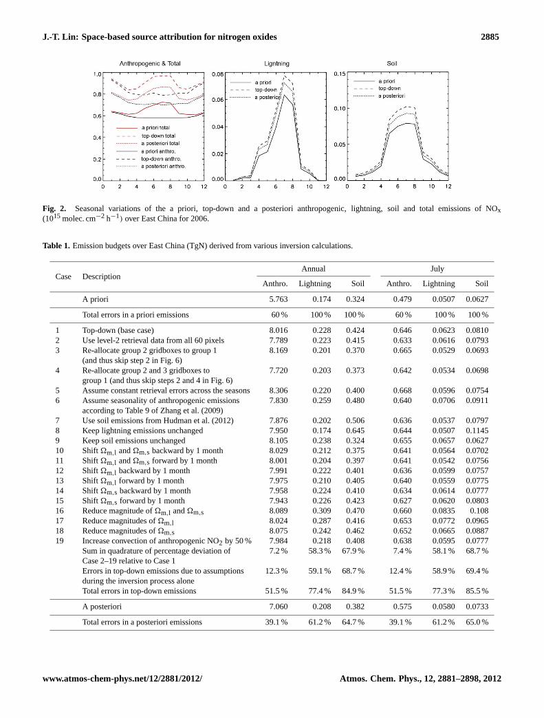
Table 1. Emission budgets over East China (TgN) derived from various inversion calculations.

Case DescriptionAnnual July

Anthro. Lightning Soil Anthro. Lightning Soil

A priori 5.763 0.174 0.324 0.479 0.0507 0.0627

Total errors in a priori emissions 60 % 100 % 100 % 60 % 100 % 100 %

1 Top-down (base case) 8.016 0.228 0.424 0.646 0.0623 0.08102 Use level-2 retrieval data from all 60 pixels 7.789 0.223 0.415 0.633 0.0616 0.07933 Re-allocate group 2 gridboxes to group 1 8.169 0.201 0.370 0.665 0.0529 0.0693

(and thus skip step 2 in Fig. 6)4 Re-allocate group 2 and 3 gridboxes to 7.720 0.203 0.373 0.642 0.0534 0.0698

group 1 (and thus skip steps 2 and 4 in Fig. 6)5 Assume constant retrieval errors across the seasons 8.306 0.220 0.400 0.668 0.0596 0.07546 Assume seasonality of anthropogenic emissions 7.830 0.259 0.480 0.640 0.0706 0.0911

according to Table 9 of Zhang et al. (2009)7 Use soil emissions from Hudman et al. (2012) 7.876 0.202 0.506 0.636 0.0537 0.07978 Keep lightning emissions unchanged 7.950 0.174 0.645 0.644 0.0507 0.11459 Keep soil emissions unchanged 8.105 0.238 0.324 0.655 0.0657 0.062710 Shift�m,l and�m,s backward by 1 month 8.029 0.212 0.375 0.641 0.0564 0.070211 Shift�m,l and�m,s forward by 1 month 8.001 0.204 0.397 0.641 0.0542 0.075612 Shift�m,l backward by 1 month 7.991 0.222 0.401 0.636 0.0599 0.075713 Shift�m,l forward by 1 month 7.975 0.210 0.405 0.640 0.0559 0.077514 Shift�m,s backward by 1 month 7.958 0.224 0.410 0.634 0.0614 0.077715 Shift�m,s forward by 1 month 7.943 0.226 0.423 0.627 0.0620 0.080316 Reduce magnitude of�m,l and�m,s 8.089 0.309 0.470 0.660 0.0835 0.10817 Reduce magnitudes of�m,l 8.024 0.287 0.416 0.653 0.0772 0.096518 Reduce magnitudes of�m,s 8.075 0.242 0.462 0.652 0.0665 0.088719 Increase convection of anthropogenic NO2 by 50 % 7.984 0.218 0.408 0.638 0.0595 0.0777

Sum in quadrature of percentage deviation of 7.2 % 58.3 % 67.9 % 7.4 % 58.1 % 68.7 %Case 2–19 relative to Case 1Errors in top-down emissions due to assumptions 12.3 % 59.1 % 68.7 % 12.4 % 58.9 % 69.4 %during the inversion process aloneTotal errors in top-down emissions 51.5 % 77.4 % 84.9 % 51.5 % 77.3 % 85.5 %

A posteriori 7.060 0.208 0.382 0.575 0.0580 0.0733

Total errors in a posteriori emissions 39.1 % 61.2 % 64.7 % 39.1 % 61.2 % 65.0 %



Table 2. Descriptions of VCDs of NO2 from individual sources derived from model simulations.

Case Description∗

1 �m Simulated by including emissions from all sources2 Simulated by including all but lightning emissions3 Simulated by including all but emissions from lightning and fertilizer associated

soil sources, i.e. only including anthropogenic, non-fertilizer soil and biomass burning sources4 Simulated by including emissions from anthropogenic and non-fertilizer soil sources only5 �m,a Simulated by including anthropogenic emissions only6 �m,l Case 1− Case 27 �m,s (Case 2− Case 3) + (Case 4− Case 5)8 �m,b Case 3− Case 4

∗ Emissions from all sources are always included for pollutants other than NOx.

3.2 Comparison between simulated and retrieved VCDsof NO2

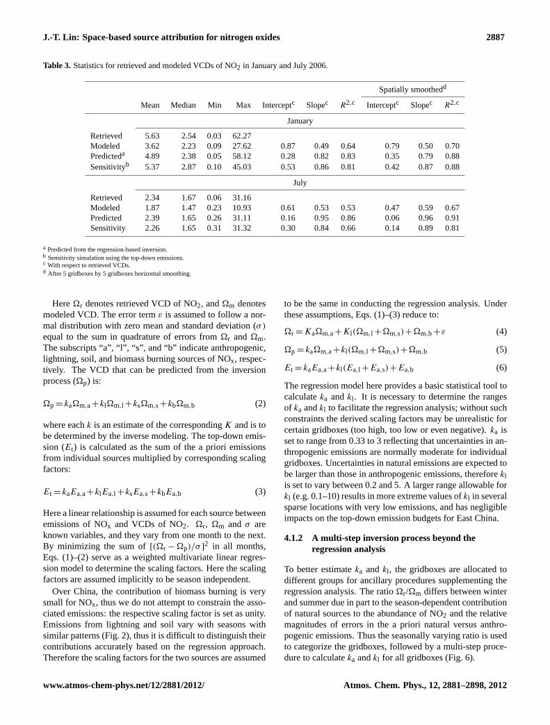
Figure 4 compares retrieved VCDs with simulated values(from all sources; Case 1 in Table 2) for January, April, July,October and annual average for 2006. Retrieved VCDs arelarge in regions with more advanced economic and industrialdevelopment and/or dense population, including the coastaland neighbor provinces from Beijing to Shanghai, the PearlRiver Delta and the Sichuan Basin. Spike values are evidentover major cities. In addition, retrieved VCDs vary acrossthe months significantly, reaching maximum values in Jan-uary and minimum values in July.

GEOS-Chem captures fairly well the spatial distributionsof retrieved VCDs in different seasons (Fig. 4). TheR2

for spatial correlation between modeled and retrieved VCDsreaches 0.64 for January and 0.53 for July (Table 3). Thesmaller correlation in July is in part because the nativehorizontal resolution of the CTM (0.667◦ long× 0.5◦ lat) isnot fine enough to capture the large spatial variation ofVCDs within short distances resulting from the short life-time of NOx (Martin et al., 2003; Lin et al., 2010a). Spa-tial smoothing of 5 gridboxes by 5 gridboxes (i.e. 1.25◦ longby 1.25◦ lat) results in a significant enhancement of model-retrieval correlation in July with theR2 increasing to 0.67.The improvement ofR2 due to the smoothing is moderate inJanuary, compared to July, since the lifetime of NOx is longerand the spatial variability of VCDs within short distances issmaller and better simulated by GEOS-Chem.

GEOS-Chem underestimates the magnitude of retrievedVCDs particularly over polluted regions in wintertime(Fig. 4). The range of simulated VCDs is also narrower thanthe retrieved range: spatially, the modeled maximum VCD islower than the retrieved maximum with the minimum beinghigher (Table 3). Averaged over East China, model VCDsare about 20 % lower than retrieved values in July and about36 % lower in January (Table 3).

4 Inversion of anthropogenic, lightning and soilemissions

4.1 Method

As discussed in Sect. 3.1, anthropogenic emissions of NOxin East China exhibit weak seasonality and natural emissionsreach maximum values in summer and minimum in winter(Fig. 2). In addition, the lifetime of NOx is shortest in sum-mer and longest in winter as a result of varying photochem-ical activity (Martin et al., 2003; Lin et al., 2010a; Lin andMcElroy, 2010). This results in minimum values in summerfor VCDs of NO2 of anthropogenic origin and maximum val-ues for NO2 from natural sources, as simulated by GEOS-Chem (Fig. 5). Averaged over East China, natural sourcescontribute to about 30 % of the total abundance of NO2 inJuly and August, in contrast to their negligible contributionsin winter months. This characteristic is exploited here to es-timate anthropogenic and natural emissions separately.

The inversion here involves a multi-step process based ona weighted multivariate linear regression analysis facilitatedby several supplementary procedures. It is done gridbox bygridbox to derive the respective emissions. The regressionis described in Sect. 4.1.1. The complete inversion processis described in Sect. 4.1.2 together with the supplementaryprocedures.

4.1.1 A weighted multivariate linear regression analysisfor each gridbox

Neglecting horizontal transport and assuming a linear rela-tionship between the total VCD of NO2 and VCDs from indi-vidual sources, the retrieved VCD of NO2 for a given gridbox(of 0.25◦ long× 0.25◦ lat) in a given month can be approxi-mated as the sum of modeled VCDs from individual emissionsources, multiplied by certain scaling factors, and a randomerror term:

�r = Ka�m,a+Kl�m,l +Ks�m,s+Kb�m,b+ε (1)

where�m =�m,a +�m,l +�m,s +�m,b.



Table 3. Statistics for retrieved and modeled VCDs of NO2 in January and July 2006.

Spatially smoothedd

Mean Median Min Max Interceptc Slopec R2,c Interceptc Slopec R2,c

January

Retrieved 5.63 2.54 0.03 62.27Modeled 3.62 2.23 0.09 27.62 0.87 0.49 0.64 0.79 0.50 0.70Predicteda 4.89 2.38 0.05 58.12 0.28 0.82 0.83 0.35 0.79 0.88Sensitivityb 5.37 2.87 0.10 45.03 0.53 0.86 0.81 0.42 0.87 0.88

July

Retrieved 2.34 1.67 0.06 31.16Modeled 1.87 1.47 0.23 10.93 0.61 0.53 0.53 0.47 0.59 0.67Predicted 2.39 1.65 0.26 31.11 0.16 0.95 0.86 0.06 0.96 0.91Sensitivity 2.26 1.65 0.31 31.32 0.30 0.84 0.66 0.14 0.89 0.81

a Predicted from the regression-based inversion.b Sensitivity simulation using the top-down emissions.c With respect to retrieved VCDs.d After 5 gridboxes by 5 gridboxes horizontal smoothing.

Here�r denotes retrieved VCD of NO2, and�m denotesmodeled VCD. The error termε is assumed to follow a nor-mal distribution with zero mean and standard deviation (σ)

equal to the sum in quadrature of errors from�r and�m.The subscripts “a”, “l”, “s”, and “b” indicate anthropogenic,lightning, soil, and biomass burning sources of NOx, respec-tively. The VCD that can be predicted from the inversionprocess (�p) is:

�p = ka�m,a+kl�m,l +ks�m,s+kb�m,b (2)

where eachk is an estimate of the correspondingK and is tobe determined by the inverse modeling. The top-down emis-sion (Et) is calculated as the sum of the a priori emissionsfrom individual sources multiplied by corresponding scalingfactors:

Et = kaEa,a+klEa,l +ksEa,s+kbEa,b (3)

Here a linear relationship is assumed for each source betweenemissions of NOx and VCDs of NO2. �r, �m and σ areknown variables, and they vary from one month to the next.By minimizing the sum of[(�r − �p)/σ ]

2 in all months,Eqs. (1)–(2) serve as a weighted multivariate linear regres-sion model to determine the scaling factors. Here the scalingfactors are assumed implicitly to be season independent.

Over China, the contribution of biomass burning is verysmall for NOx, thus we do not attempt to constrain the asso-ciated emissions: the respective scaling factor is set as unity.Emissions from lightning and soil vary with seasons withsimilar patterns (Fig. 2), thus it is difficult to distinguish theircontributions accurately based on the regression approach.Therefore the scaling factors for the two sources are assumed

to be the same in conducting the regression analysis. Underthese assumptions, Eqs. (1)–(3) reduce to:

�r = Ka�m,a+Kl(�m,l +�m,s)+�m,b+ε (4)

�p = ka�m,a+kl(�m,l +�m,s)+�m,b (5)

Et = kaEa,a+kl(Ea,l +Ea,s)+Ea,b (6)

The regression model here provides a basic statistical tool tocalculateka andkl . It is necessary to determine the rangesof ka andkl to facilitate the regression analysis; without suchconstraints the derived scaling factors may be unrealistic forcertain gridboxes (too high, too low or even negative).ka isset to range from 0.33 to 3 reflecting that uncertainties in an-thropogenic emissions are normally moderate for individualgridboxes. Uncertainties in natural emissions are expected tobe larger than those in anthropogenic emissions, thereforeklis set to vary between 0.2 and 5. A larger range allowable forkl (e.g. 0.1–10) results in more extreme values ofkl in severalsparse locations with very low emissions, and has negligibleimpacts on the top-down emission budgets for East China.

4.1.2 A multi-step inversion process beyond theregression analysis

To better estimateka andkl , the gridboxes are allocated todifferent groups for ancillary procedures supplementing theregression analysis. The ratio�r/�m differs between winterand summer due in part to the season-dependent contributionof natural sources to the abundance of NO2 and the relativemagnitudes of errors in the a priori natural versus anthro-pogenic emissions. Thus the seasonally varying ratio is usedto categorize the gridboxes, followed by a multi-step proce-dure to calculateka andkl for all gridboxes (Fig. 6).



37

1

Figure 3. 2 Fig. 3. (a)Seasonal variations of monthly mean near-surface (2 m)air temperature and precipitation observed from 284 meteorologicalstations over East China and modeled by GEOS-5. The observationdata are taken from the global hourly dataset (DS3505) archivedin the National Oceanic and Atmospheric Administration (NOAA)National Climatic Data Center (NCDC) (http://www7.ncdc.noaa.gov/CDO/cdo; see Lin et al., 2010b). Data from GEOS-5 are sam-pled at the meteorolgocal stations for consistency with the obser-vations. (b) Spatial distribution of the month-to-month correla-tion between a priori anthropogenic and natural (lightning + soil)emissions.

Gridboxes are assigned to group 1 if the ratio�r/�m for aselected winter month is smaller than the ratio for a selectedsummer month; otherwise they are assigned to group 2. Forgridboxes in group 1, the regression analysis is performed tocalculateka andkl (step 1 in Fig. 6). Results are discarded ifthe regression is not statistically significant at a significancelevel of 0.1 under the Chi-square test. Spatial interpolation(step 2 in Fig. 6) is then conducted iteratively to derivekl forall gridboxes: for a gridbox with undeterminedkl , the value

of kl is calculated as the geometric mean of values in the sur-rounding 24 gridboxes derived previously. For gridboxes ingroup 2, the regression analysis usually results in unrealisti-cally low values forkl and thus is used to estimateka only(step 3 in Fig. 6); the value ofkl has been determined at pre-vious steps. Again, the result is discarded if the regression isnot statistically significant.

The regression approach may not be appropriate for cer-tain gridboxes with unrealistically large�r/�m ratios in thewinter month. This is because the scaling factorka likely hasa significant seasonal dependence as a result of the seasonal-ity in anthropogenic emissions not fully accounted for in thea priori dataset. These gridboxes are therefore reassigned to athird group, where aka is derived for each month as the ratio[�r − kl(�m,l +�m,s)−�m,b]/�m,a (step 4 in Fig. 6). Ten-tatively, a gridbox is allocated to group 3 if the ratio�r/�mexceeds 3, or if the ratio exceeds 2 with�r being higher than6× 1015 molec. cm−2, in the winter month.

As a final step, spatial interpolation is conducted to obtainka for gridboxes of groups 1 and 2 where the regression is notstatistically significant (step 5 in Fig. 6).

In group allocation and subsequent inversion process, eachof three winter months (December, January and February) ispaired with each of two summer months (July and August)to generate a suite of six cases for winter-summer contrast.(June is not selected since the contribution of natural sourcesto the total abundance of NO2 is not as significant as that inJuly or August). Results from the six cases are combinedto obtain final values ofka and kl . Specifically, results ata given step available from any or all of the six cases aregeometrically averaged to obtain final values ofka andkl , ifand only if they have not been derived at earlier steps.

4.2 Scaling factors estimated for anthropogenic,lightning and soil sources

The scaling factors are determined at step 1 for most grid-boxes (Figs. 7 and 8). At this step, the values ofka are aroundunity in most areas, are consistently larger than 1 over thesouthwestern provinces, and vary between 1 and 2 in manyof the remaining areas (Fig. 7). By comparison,kl variesmore significantly from one location to the next (Fig. 8). Itreaches maximum values in southern Hebei Province andalong the northern coasts of the Bohai Sea, which are at-tributable in part to an underestimate in fertilizer-associatedsoil emissions in the a priori dataset (see Sect. 4.4 for de-tails). The value ofkl also has spike values at spotty locationsin other parts of East China where natural emissions are nor-mally very low. These spikes are likely artificial results ofthe inversion algorithm, errors in GEOS-Chem, and/or errorsin the satellite product; they however have negligible impactson emission budgets over East China.


http://www7.ncdc.noaa.gov/CDO/cdo

http://www7.ncdc.noaa.gov/CDO/cdo


38

1

Figure 4. 2

3

4

5

6

7

8

Fig. 4. VCDs of NO2 (1015molec. cm−2) for January, April, July, October and annual average for 2006 retrieved from OMI, simulated byGEOS-Chem with a priori emissions, predicted by the inversion approach, and simulated by GEOS-Chem with top-down emissions. Areasoutside the territory of China or without valid retrievals are shown in grey.



39

1

Figure 5. 2

3

4

5

6

7

8

9

10

11

12

13

14

15

16

17

18

19

20

Fig. 5. Seasonal variations of VCDs of NO2 (1015molec. cm−2) over East China for 2006 resulting from anthropogenic, lightning, soiland total emissions of NOx modeled by GEOS-Chem and predicted by the inversion. Also included is the seasonality of VCDs retrievedfrom OMI.

40

1

Figure 6. 2

3 Fig. 6. Description of the regression-based step-by-step inversionprocess after gridbox grouping. Values ofkl are determined atsteps 1 and 2 for all gridboxes andka at steps 1, 3, 4, 5. SeeSect. 4.1.2 for detailed analysis.

The special treatment at step 4 is taken mainly for grid-boxes in and around Shanxi Province and in parts of Ningxiaand Inner-Mongolia (Fig. 7). These places are main areas inChina for coal mining and coal-fired electricity generation.The large values ofka in these places, particularly in win-ter, suggest that the a priori dataset from INTEX-B likelyunderestimates anthropogenic sources related to use of coal,consistent with the findings of Wang et al. (2010).

The final values ofka andkl are determined at step 5 (seeFig. 7 for January) and step 2 (Fig. 8), respectively, for allgridboxes. They are used to calculate the top-down emis-sions for respective sources.

4.3 VCDs of NO2 predicted from the inversion process

Compared to simulation results, predicted VCDs are muchcloser to retrieved values (Fig. 4). The spatial correlationbetween predicted and retrieved VCDs is much higher thanthe correlation between simulated and retrieved VCDs, withthe R2 increasing from 64 % to 83 % in January and from53 % to 86 % in July (Table 3). Averaged over East China,predicted VCDs are within 15 % of retrieved values acrossthe seasons.

4.4 Top-down emissions

Figure 9 compares the top-down emissions of NOx for an-thropogenic, lightning and soil sources with respective a pri-ori emissions for July. Both top-down and a priori datasetssuggest significant anthropogenic sources over the coastalprovinces from Shanghai to Beijing and over the Pearl RiverDelta, resulting in large concentrations of NO2 (Fig. 10). Thetop-down anthropogenic emissions are much higher than thea priori emissions in cities and at locations with extensive useof coal, especially in the northern provinces.

In July, emissions from lightning are large in the north asa result of strong convection events associated with the sum-mer monsoon (Fig. 9). Soil emissions are greatest in ma-jor agricultural areas in Hebei, Henan, Shandong and partsof neighbor provinces (Fig. 9). The top-down estimates forlightning and soil emissions are much larger than the a pri-ori values at many places of the respective source regions.In particular, the significant increases in soil emissions oversouthern Hebei and along the northern coasts of the BohaiSea are not likely to be an artificial result of assumptionsembedded in the inversion process, as they persist duringvarious sensitivity tests (Cases 1–19 in Table 1). The in-creases are consistent with the new bottom-up estimates bySteinkamp and Lawrence (2011) and Hudman et al. (2012),and are contributed in part by the intensive fertilizer-derivedemissions that are underestimated in GEOS-Chem (Yienger



41

1

Figure 7. 2

3

4

5

6

7

Fig. 7. Scaling factors for anthropogenic emissions (ka) determined at steps 1, 3, 4 and 5 of the inversion process described in Fig. 6 andSect. 4.1.2. Step 2 does not affectka and thus is not presented. Results at steps 4 and 5 are for January in particular. Areas outside theterritory of China or with undeterminedka are shown in grey.

42

1

Figure 8. 2

3

4

5

6

7

8

9

10

11

12

13

14

15

16

17

18

Fig. 8. Scaling factors for lightning/soil emissions (kl ) determined at steps 1 and 2 of the inversion process described in Fig. 6 and Sect. 4.1.2.These two steps decidekl for all gridboxes. Areas outside the territory of China or with undeterminedkl are shown in grey.

and Levy, 1995; Wang et al., 1998; Steinkamp and Lawrence,2011). More detailed comparisons with Steinkamp andLawrence (2011) and Hudman et al. (2012) are conductedin Sect. 5.1.2.

The contribution of anthropogenic sources to the totalemissions of NOx in July is generally consistent between thea priori and top-down datasets (Fig. 9). The anthropogeniccontribution exceeds 80 % over large areas of East China,but is lower than 60 % over most of the northwest and Inner-Mongolia. It differs from the anthropogenic contribution to

the VCD of NO2 (Fig. 10). This is in part because lightningemissions occur at higher altitudes with longer lifetime ofNOx than near the ground, compensated by a reduced frac-tion of NO2 in NOx. Another factor is the use of averag-ing kernel in deriving model VCDs. The averaging kernelis larger for NO2 of lightning origin at higher altitudes andlower for NO2 derived from the ground (Eskes and Boersma,2003). Thus the contribution is enhanced for a given amountof lightning emissions to the total abundance of NO2, com-pared to the same amount of emissions from the ground. The



43

1

Figure 9. 2

3

4

5

6

7

8

9

10

11

12

13

14

Fig. 9. The a priori, top-down and a posteriori estimates of anthropogenic, lightning and soil emissions of NOx (1015molec. cm−2 h−1) andthe anthropogenic contributions (in percentage) to total emissions for July 2006 over East China. Areas outside the territory of China areshown in grey.

effect is evident particularly over the southwest. The in-verse modeling study by Lin et al. (2010a) showed that anassumed 100 % increase (0.57 TgN yr−1) in top-down light-ning emissions resulted in a 15 % reduction (0.86 TgN yr−1)

in top-down anthropogenic emissions for July 2008 over EastChina; that is, any NO2 molecule originating from lightningis 1.5 times as likely to be observed by OMI than a NO2molecule of anthropogenic origin, consistent with the analy-sis here. In addition, data for simulated VCDs are sampledat the time of day of satellite overpass from days with validretrieval data; while data for monthly emissions are averagedover all time of day in all days of the month. The differ-ent sampling methods and the day-to-day and diurnal vari-ations in natural emissions may introduce some differencesbetween anthropogenic contributions to total emissions andto total VCDs. Another possible cause is the neglect of hori-zontal transport likely introducing uncertainties in source at-tribution for relatively clean regions, e.g. at many places ofInner-Mongolia.

Table 1 compares the a priori and top-down emission bud-gets over East China for individual sources. Annually, theinversion results in budgets of 8.016 TgN, 0.228 TgN and

0.424 TgN for anthropogenic, lightning and soil emissions,respectively. These values are about 39 %, 31 % and 31 %larger than the corresponding a priori estimates. The top-down datasets also suggest that both lightning and soil emis-sions are less than 6 % of anthropogenic emissions. For July,the top-down budgets for lightning and soil emissions are0.0623 TgN and 0.0810 TgN, respectively, about 10 % and13 % of anthropogenic emissions estimated at 0.646 TgN.

4.5 Improved GEOS-Chem simulations using thetop-down emissions

The inversion approach presented here assumes a linear rela-tionship for a given gridbox between the total VCD of NO2and VCDs from individual sources and between emissions ofNOx and VCDs of NO2. It also neglects horizontal transport,which may introduce uncertainties in deriving emissions forindividual gridboxes. To evaluate the reliability of the in-version results, sensitivity simulations of GEOS-Chem wereconducted for January and July 2006 by using the top-downemissions to drive the CTM. As shown in Fig. 4, VCDs re-sulting from the sensitivity simulations reproduce the spatial



44

1

Figure 10. 2 Fig. 10. VCDs of NO2 (1015molec. cm−2) in July 2006 over East China resulting from anthropogenic, lightning and soil emissions ofNOx and the anthropogenic contributions (in percentage) to the total VCDs modeled by GEOS-Chem and predicted by the inversion. Areasoutside the territory of China or without valid retrievals are shown in grey.

distribution of retrieved VCDs in both months. TheR2 forspatial correlation reaches a high level of 81 % for Januaryand 66 % for July (Table 3). The smaller correlation in Julyis due to the short lifetime of NOx such that the CTM (at0.667◦ long× 0.5◦ lat) is not able to simulate the large spa-tial variation of NO2 within short distances, as discussedin Sect. 3.2. After (5 gridboxes by 5 gridboxes) horizontalsmoothing, theR2 increases to 88 % for January and 81 %for July (Table 3). Averaged over East China, the magnitudeof model VCD is about 10 % higher than the predicted valuein January and about 5 % lower in July (Table 3), indicatinga slight nonlinear relationship between emissions and VCDsthrough the impacts on other species (HOx, ozone, etc.) andconsequently on the lifetime of NOx and its partitioning intoNO and NO2.

4.6 Sensitivity of emission inversion to embeddedassumptions

This section evaluates the effects on the top-down emissionsof several important assumptions taken during the inversionprocess, particularly for assumptions on the seasonality ofvarious emission sources. The results are summarized inTable 1.

This study only includes 30 out of the 60 pixels from eachOMI scan with smaller sizes in order to better analyze thespatial distribution of nitrogen within short distances. Thetop-down emission budgets for individual sources are similarto results from a sensitivity calculation employing OMI datafrom all pixels (Case 2 in Table 1); the differences are largerfor individual locations (not shown).

The inversion approach allocates individual gridboxes tothree groups prior to the regression. The effect of group allo-cation was evaluated by two tests, one by re-allocating grid-boxes in group 2 to group 1 and the other by re-allocatinggridboxes in both group 2 and group 3 to group 1. The testssuggested that the effect of group allocation is less than 15 %for top-down lightning/soil emission budgets for East China(Cases 3 and 4 in Table 1) with much larger impacts for indi-vidual locations (not shown).

The regression accounts for the seasonal dependence ofretrieval errors. A sensitivity test assuming a time invari-ant relative error of 30 % resulted in decreases by less than5 % in top-down lightning/soil emissions (Case 5 in Table 1).Therefore the inversion approach is not sensitive to the sea-sonality of retrieval errors assumed here.

The regression here relies on assumptions on the seasonalvariations of individual emission sources. Anthropogenicemissions from power plants, industry and transportationdiffer slightly among seasons (Zhang et al., 2009), but areassumed here to be season independent for simulations ofGEOS-Chem. The assumption was evaluated by a sensi-tivity analysis taking into account the seasonality estimatedby Zhang et al. (2009). Specifically, modeled anthropogenicVCDs (�m,a) for individual months were scaled prior to theinversion by the seasonality of total anthropogenic emissionsderived from Table 9 of Zhang et al. (2009). This resulted inincreases by less than 15 % in top-down lightning/soil emis-sions (Case 6 in Table 1). The effect is smaller than 5 % fortop-down anthropogenic emissions.



Another test was taken to evaluate the effect of errors in theYienger and Levy (1995) soil emissions used as our a prioriestimate. Specifically, the updated emission data by Hudmanet al. (2012) (see Sect. 5.1.2 for specifications) were usedto adjust modeled VCDs from soil sources (�m,s) prior tothe inversion, by scaling the VCDs for individual gridboxeswith the ratios of Hudman et al. (2012) over Yienger andLevy (1995) soil emissions. As such, the annual top-downlightning emissions were reduced by 11 % and soil emissionsenhanced by 19 % (Case 7 in Table 1). This is because of dif-ferences in seasonality (timing and magnitude) between soilemissions estimated by Hudman et al. (2012) and by Yiengerand Levy (1995). The impacts of emission seasonality areanalyzed further below.

Jaegle et al. (2005), Wang et al. (2007) and Zhao andWang (2009) assumed lightning emissions to be simulatedwell by the CTM with no attempt to constrain them inversely.Under the same assumption, a sensitivity analysis was con-ducted by keeping lightning emissions unchanged during theinversion process here. This resulted in a 52 % increase inthe top-down soil emission budget on the annual basis and a41 % increase for July (Case 8 in Table 1).

If soil emissions are held unchanged during the inversionprocess, the top-down lightning emissions will be increasedby less than 6 % (Case 9 in Table 1).

The inversion relies on modeled seasonal variations oflightning and soil emissions for separation from anthro-pogenic emissions. Due to similarity in seasonality, light-ning and soil sources cannot be separated unambiguously fora given gridbox. A total of nine additional tests were per-formed to further analyze the sensitivity of inversion resultsto assumptions on the seasonality of lightning and soil emis-sions, including the timing and magnitude (Cases 10–18 inTable 1). To test the timing of the seasonality,�m,l and�m,swere shifted arbitrarily forward or backward by one month,separately or in combination, prior to the inversion process(Cases 10–15 in Table 1). As a result, top-down lightningand soil emissions are affected by up to 14 % on the regionalmean basis. Another three tests evaluate the magnitude ofthe seasonality, by lowering�m,l and�m,s, separately andin combination, by 20 % in spring (March, April, May) andfall (September, October, November) and 40 % in summer(June, July, August). These changes have significant impactson top-down lightning and soil emissions: by reducing�m,land�m,s simultaneously, top-down lightning and soil emis-sions were enhanced by about 33–34 % in July.

Convection lifts pollutants in the boundary layer to the up-per troposphere affecting the vertical distributions of vari-ous species. The magnitude of convection is highly param-eterized in current climate models and CTMs and thus con-tains large uncertainties (Tost et al., 2010). The importanceof model convection for simulated VCDs of NO2 originatesfrom the altitude dependences of the lifetime of NOx, thefraction of NO2 in NOx, and the averaging kernel that is ap-plied to the vertical distribution of NO2 (when comparing

with satellite retrievals). Its net effect can be estimatedroughly by comparing NO2 originating from a given amountof lightning emissions (i.e. located mostly at high altitudes)and NO2 from the same amount of anthropogenic emissions(i.e. located mostly in the boundary layer). As suggestedby Lin et al. (2010a) and discussed in detail in Sect. 4.4,any NO2 molecule originating from lightning is 1.5 times aslikely to be observed by OMI than a NO2 molecule of anthro-pogenic origin for July 2008 over East China. Thus, doublingthe magnitude of model convection and consequent changesin vertical distribution of NO2 will result in a net increase by50 % in modeled convection-associated VCD of NO2 (whenthe averaging kernel is taken into account). To evaluate theimpact of potential errors in model convection, a sensitivitytest enhanced by 50 % the magnitude of convection of an-thropogenic NO2 in July and August 2006, by tentatively in-creasing by 25 % modeled concentrations of anthropogenicNO2 above 500 hPa (Case 19 in Table 1). This effectivelyincreased modeled anthropogenic VCDs of NO2 over EastChina by about 7.5 % in both months. It consequently re-sulted in a slight reduction in top-down anthropogenic emis-sions with reductions by about 4–5 % in top-down lightningand soil emissions (Case 19 in Table 1).

Errors in top-down emissions attributable to the inversionprocedure are calculated as the sum in quadrature of percent-age deviations of all inversion results (Cases 2–19) relative tothe base estimate (Case 1), added in quadrature with errorsresulting from the nonlinearity between emissions of NOxand VCDs of NO2 that are not accounted for in the sensi-tivity tests. The nonlinearity derived errors are taken to beabout 10 % for East China as a whole, based on discussionsin Sect. 4.5. Thus, errors in top-down emissions for EastChina attributed to the inversion procedure are estimated tobe about 12 %, 59 % and 69 % for anthropogenic, lightningand soil sources, respectively (Table 1).

4.7 Total errors in the top-down emission budgets overEast China

The inverse estimate here is subject to errors in retrievals,errors in model simulations, and errors in the inversion pro-cedures as estimated from the sensitivity analyses. The totalerror in top-down emission budget over East China is takento be the sum in quadrature of the three errors, amounting toabout 52 %, 77 % and 85 % for anthropogenic, lightning andsoil sources, respectively (Table 1).

We do not attempt to estimate the total errors for individ-ual gridboxes as the model and retrieval errors available hereonly represent bulk estimates on the regional mean basis.



5 A posteriori emissions

The a posteriori emissions are estimated as the averageof the a priori and top-down emissions weighted by theinverse-square of their respective errors (Martin et al., 2003).Errors in the a priori emissions are taken to be 60 % for an-thropogenic sources (Wang et al., 2007; Zhao and Wang,2009) increasing to 100 % for lightning and soil sources ac-counting for the large range of current estimates (Boersmaet al., 2005; Jaegle et al., 2005; Schumann and Huntrieser,2007; Wang et al., 2007; Zhao and Wang, 2009; Lin etal., 2010a). Errors in the respective top-down emissions aretaken to be 52 %, 77 % and 85 %, as derived in Sect. 4.7.Note that the error estimates here are conducted for totalemissions in East China. Errors at individual locations maybe much larger for both a priori and top-down datasets; thederivation however requires more detailed information thatis not available currently. Therefore the error estimates forregional emission budgets are applied to individual loca-tions, as a simplified procedure, in deriving the a posterioriemissions.

The a posteriori emissions for 2006 over East Chinaamount to 7.060 TgN (±39 %) for anthropogenic sources, to0.208 TgN (±61 %) for lightning sources, and to 0.382 TgN(±65 %) for soil sources (Table 1). For July, the a posterioribudgets are 0.575 TgN (±39 %), 0.0580 TgN (±61 %), and0.0733 TgN (±65 %), respectively. The temporal and spatialdistributions of the a posteriori emissions are presented inFigs. 2 and 9 for comparison with the a priori and top-downemissions.

5.1 Comparison with previous estimates

That anthropogenic emissions inferred from space are largerthan bottom-up inventories for China is consistent with re-sults from many previous studies (Jaegle et al., 2005; Wanget al., 2007; Zhang et al., 2007; Lin and McElroy, 2011). Oura posteriori budget for anthropogenic emissions over EastChina is similar to the value of 0.565 TgN for July 2007 es-timated by Zhao and Wang (2009). This study further pin-points, at a higher resolution, cities and areas with extensiveuse of coal to be the main regions where bottom-up inven-tories likely underestimate anthropogenic emissions. Eval-uation of lightning emissions is more difficult due to thelarge uncertainty in current research (Boersma et al., 2005;Schumann and Huntrieser, 2007) and the significant interan-nual variability of lightning occurrences on the regional scale(Schumann and Huntrieser, 2007). Our a posteriori emis-sions are within the range of previous estimates (Boersma etal., 2005; Schumann and Huntrieser, 2007; Stavrakou et al.,2008).

Soil emissions of NOx over China are of great interest con-cerning the extensive use of fertilizers. A detailed analysisis conducted as follows for our a posteriori estimate of soilemissions.

5.1.1 Comparison with previous satellite-derived soilemission estimates

Wang et al. (2007) suggested that soil emissions are about0.85 TgN per year for 1997–2000 over East China, amount-ing to 23 % of anthropogenic emissions on the annual ba-sis and to as much as 43 % for summer months. In bet-ter agreement with our estimates for East China, Jaelge etal. (2005) found an annual budget of∼0.40 TgN for 2000,and Zhao and Wang (2009) suggested soil emissions to beabout 0.0883 TgN for July 2007 (L. Jaegle, personal commu-nication, 2011; C. Zhao and Y. Wang, personal communica-tion, 2011). The differences are derived mainly from satelliteproducts and methods to separate anthropogenic and naturalsources of NOx employed in individual studies.

5.1.2 Comparison with recent bottom-up estimates forsoil emissions

Two new bottom-up estimates have been conducted for soilemissions by Steinkamp and Lawrence (2011) and Hud-man et al. (2012), improving upon the work of Yienger andLevy (1995) used as our a priori emissions. The new esti-mates employ information from more recent and completefield measurements to estimate emission factors. They usesoil moisture rather than precipitation amount to separatedry and wet soil conditions. Hudman et al. (2012) also usesoil moisture to calculate the duration and strength of theN-pulsing. The two new estimates include updated infor-mation on fertilizer use and vegetation map. For fertilizeruse, Steinkamp and Lawrence (2011) account for its interan-nual variation based on the FAO statistics; while Hudman etal. (2012) use the latest available gridded dataset from Pot-ter et al. (2010) representative of the year 2000. The twostudies assume about 1.0 % and 0.62 %, respectively, of ni-trogen in fertilizers to be emitted as NOx, for better com-parisons with the observation-based estimate by Stehfest andBouwman (2006). Hudman et al. (2012) combine satellitemeasurements for the growing season of vegetation and at-tribute 75 % of fertilizer derived emissions to the first monthof the growing season. They also consider deposited nitro-gen species as an additional fertilizer-like source of NOx.Steinkamp and Lawrence (2011) update the leaf area index(LAI) data for calculating the canopy reduction factor; whileHudman et al. (2012) assume no canopy reduction.

Our a posteriori soil emissions at 0.382 TgN (±65 %) an-nually is within 25 % of the value of 0.504 TgN calculated byHudman et al. (2012), if canopy reduction is accounted for intheir estimate (R. Hudman, personal communication, 2011).Our emissions are also within the range of 0.18–0.97 TgNsuggested by Steinkamp and Lawrence (2011) (see their Ta-ble 7). In addition, the horizontal distribution of soil emis-sions is in broad agreement between our a posteriori datasetand the two new bottom-up estimates.



6 Conclusions

A regression-based multi-step inversion approach is pro-posed to estimate emissions of NOx from anthropogenic,lightning and soil sources for 2006 over East China on a0.25◦ long× 0.25◦ lat grid. It exploits information on VCDsof tropospheric NO2 retrieved from the OMI instrument byKNMI (the DOMINO product version 2). The nested GEOS-Chem model for East Asia is used to interpret the impacts ofindividual sources on VCDs of NO2 to facilitate the inver-sion analysis. The inversion is conducted gridbox by grid-box to derive the respective emissions. For any given grid-box, anthropogenic and natural sources are separated basedon their different seasonality; and lightning and soil emis-sions are considered together due to their similarity in sea-sonality. Differences in spatial patterns between lightningand soil emissions are used implicitly for source separationto some extent.

The inversion starts by allocating the gridboxes to threegroups based on analyses of the ratio of retrieved over mod-eled VCDs in winter and summer. A multivariate regres-sion analysis is used then to derive emissions from individ-ual sources for all months, taking advantage of the seasonalpatterns of different sources determined by the CTM. Ancil-lary procedures are taken to supplement the regression anal-ysis for gridboxes in different groups. Assumptions madeduring the inversion process contribute to errors in the top-down emission budgets for East China by∼12 % for anthro-pogenic sources,∼59 % for lightning sources and∼69 % forsoil sources. Sensitivity simulations of GEOS-Chem drivenby the top-down emission data reproduce the spatial distri-bution of VCDs retrieved from OMI, with theR2 for spatialcorrelation reaching 0.88 for January and 0.81 for July after(5 gridboxes by 5 gridboxes) horizontal smoothing.

The inversion results in an annual budget of 7.060 TgN(±39 %) for the a posteriori anthropogenic emissions of NOxover East China, about 23 % larger than the INTEX-B dataset(Zhang et al., 2009) used as our a priori emissions. Onthe 0.25◦ long× 0.25◦ lat grid, it is evident that the excessis greater over cities and areas with extensive use of coal,particularly in the north in winter.

The a posteriori budgets are 0.208 TgN (±61 %) and0.382 TgN (±65 %) for lightning and soil emissions, respec-tively, for 2006 over East China. Both values are about18 % higher than the respective a priori estimates, but areeach less than 6 % of the a posteriori anthropogenic emis-sions. Even for July, the a posteriori lightning and soilemissions are only about 10 % and 13 % of anthropogenicemissions, respectively. Our results for soil emissions areconsistent with recent bottom-up estimates by Steinkampand Lawrence (2011) and Hudman et al. (2012) and previ-ous inverse estimates by Jaegle et al. (2005), Stavrakou etal. (2008) and Zhao and Wang (2009). They are howeverabout half of the inverse estimate by Wang et al. (2007) who

suggested soil emissions to be more than 40 % of anthro-pogenic emissions in summer of 1997–2000.

In concluding, anthropogenic emissions are found to bethe dominant source of NOx over East China for 2006, evenin summer when natural sources reach maximum values. Thecontribution of anthropogenic emissions most likely has in-creased in more recent years due to their rapid growth (Linand McElroy, 2011). In the future, the anthropogenic con-tribution may continue to increase along with the rapid eco-nomic and industrial development, if emission control is nottaken successfully. The importance of nitrogen control hasbeen recognized by the Chinese government, resulting incontrol strategies targeting the power sector. However, thesuccessfulness of nitrogen control also depends on changesin emissions from other sectors, particularly the industrialsector for which the current inventories may be subject tomuch larger uncertainties than for the power sector (Zhao etal., 2011). Further research is required to evaluate the ef-fectiveness of nitrogen control and resulting impacts on thecontributions of anthropogenic versus natural sources to at-mospheric nitrogen burdens.

Acknowledgements.This research is supported by the NationalNatural Science Foundation of China, grant 41005078 and41175127. We acknowledge the free use of tropospheric NO2column data fromwww.temis.nl.

Edited by: A. Richter

References

Allen, D. J. and Pickering, K. E.: Evaluation of lightning flash rateparameterizations for use in a global chemical transport model,J. Geophys. Res., 107, 4711,doi:10.1029/2002jd002066, 2002.

Boersma, K. F., Eskes, H. J., Meijer, E. W., and Kelder, H. M.: Esti-mates of lightning NOx production from GOME satellite obser-vations, Atmos. Chem. Phys., 5, 2311–2331,doi:10.5194/acp-5-2311-2005, 2005.

Boersma, K. F., Eskes, H. J., Veefkind, J. P., Brinksma, E. J., vander A, R. J., Sneep, M., van den Oord, G. H. J., Levelt, P. F.,Stammes, P., Gleason, J. F., and Bucsela, E. J.: Near-real timeretrieval of tropospheric NO2 from OMI, Atmos. Chem. Phys.,7, 2103–2118,doi:10.5194/acp-7-2103-2007, 2007.

Boersma, K. F., Eskes, H. J., Dirksen, R. J., van der A, R. J.,Veefkind, J. P., Stammes, P., Huijnen, V., Kleipool, Q. L., Sneep,M., Claas, J., Leitao, J., Richter, A., Zhou, Y., and Brunner, D.:An improved tropospheric NO2 column retrieval algorithm forthe Ozone Monitoring Instrument, Atmos. Meas. Tech., 4, 1905–1928,doi:10.5194/amt-4-1905-2011, 2011.

Chen, D., Wang, Y., McElroy, M. B., He, K., Yantosca, R. M., andLe Sager, P.: Regional CO pollution and export in China simu-lated by the high-resolution nested-grid GEOS-Chem model, At-mos. Chem. Phys., 9, 3825–3839,doi:10.5194/acp-9-3825-2009,2009.

Eskes, H. J. and Boersma, K. F.: Averaging kernels for DOAS total-column satellite retrievals, Atmos. Chem. Phys., 3, 1285–1291,


www.temis.nl

http://dx.doi.org/10.1029/2002jd002066

http://dx.doi.org/10.5194/acp-5-2311-2005



http://dx.doi.org/10.5194/amt-4-1905-2011



2003,http://www.atmos-chem-phys.net/3/1285/2003/.

Hudman, R. C., Jacob, D. J., Turquety, S., Leibensperger, E. M.,Murray, L. T., Wu, S., Gilliland, A. B., Avery, M., Bertram, T.H., Brune, W., Cohen, R. C., Dibb, J. E., Flocke, F. M., Fried,A., Holloway, J., Neuman, J. A., Orville, R., Perring, A., Ren,X., Sachse, G. W., Singh, H. B., Swanson, A., and Wooldridge,P. J.: Surface and lightning sources of nitrogen oxides over theUnited States: Magnitudes, chemical evolution, and outflow, J.Geophys. Res., 112, D12S05,doi:10.1029/2006jd007912, 2007.

Hudman, R. C., Moore, N. E., Martin, R. V., Russell, A. R., Mebust,A. K., Valin, L. C., and Cohen, R. C.: A mechanistic modelof global soil nitric oxide emissions: implementation and spacebased-constraints, Atmos. Chem. Phys. Discuss., 12, 3555–3594,doi:10.5194/acpd-12-3555-2012, 2012.

Huntrieser, H., Schlager, H., Holler, H., Schumann, U., Betz, H.D., Boccippio, D., Brunner, D., Forster, C., and Stohl, A.: Light-ning produced NOx in tropical, subtropical and midlatitude thun-derstorms: New insights from airborne and lightning observa-tions, Geophys. Res. Abstr., EGU2006-A-03286, EGU GeneralAssembly 2006, Vienna, Austria, 2006.

Jaegle, L., Steinberger, L., Martin, R. V., and Chance, K.: Globalpartitioning of NOx sources using satellite observations: Relativeroles of fossil fuel combustion, biomass burning and soil emis-sions, Faraday Discuss., 130, 407–423,doi:10.1039/b502128f,2005.

Lin, J.-T. and McElroy, M. B.: Impacts of boundary layer mixingon pollutant vertical profiles in the lower troposphere: Impli-cations to satellite remote sensing, Atmos. Environ., 44, 1726–1739,doi:10.1016/j.atmosenv.2010.02.009, 2010.

Lin, J.-T. and McElroy, M. B.: Detection from space of a reductionin anthropogenic emissions of nitrogen oxides during the Chi-nese economic downturn, Atmos. Chem. Phys., 11, 8171–8188,doi:10.5194/acp-11-8171-2011, 2011.

Lin, J.-T., McElroy, M. B., and Boersma, K. F.: Constraint ofanthropogenic NOx emissions in China from different sectors:a new methodology using multiple satellite retrievals, Atmos.Chem. Phys., 10, 63–78,doi:10.5194/acp-10-63-2010, 2010a.

Lin, J.-T., Nielsen, C. P., Zhao, Y., Lei, Y., Liu, Y., and McEl-roy, M. B.: Recent Changes in Particulate Air Pollution overChina Observed from Space and the Ground: Effectivenessof Emission Control, Environ. Sci. Technol., 44, 7771–7776,doi:10.1021/es101094t, 2010b.

Martin, R. V., Jacob, D. J., Chance, K., Kurosu, T. P., Palmer, P.I., and Evans, M. J.: Global inventory of nitrogen oxide emis-sions constrained by space-based observations of NO2 columns,J. Geophys. Res., 108, 4537,doi:10.1029/2003JD003453, 2003.

Martin, R. V., Sioris, C. E., Chance, K., Ryerson, T. B., Bertram,T. H., Wooldridge, P. J., Cohen, R. C., Neuman, J. A., Swanson,A., and Flocke, F. M.: Evaluation of space-based constraints onglobal nitrogen oxide emissions with regional aircraft measure-ments over and downwind of eastern North America, J. Geophys.Res., 111, D15308,doi:10.1029/2005JD006680, 2006.

Moorthi, S. and Suarez, M. J.: Relaxed Arakawa-Schubert – A Pa-rameterization of moist convection for general-circulation mod-els, Mon. Weather Rev., 120, 978–1002, 1992.

Muller, J.-F. and Stavrakou, T.: Inversion of CO and NOx emissionsusing the adjoint of the IMAGES model, Atmos. Chem. Phys., 5,1157–1186,doi:10.5194/acp-5-1157-2005, 2005.

Murray, L. T., Jacob, D. J., Logan, J. A., and Koshak, W.: Improv-ing techniques for satellite-based constraints on the lightning pa-rameterization in a global chemical transport model, 11th Con-ference on Atmospheric Chemistry, January 14, 2009.

Murray, L. T., Jacob, D. J., and Logan, J. A.: Investigatinglightning-driven interannual variability in the oxidative capac-ity of the troposphere, Geophys. Res. Abstr., EGU2010-14332,EGU General Assembly 2010, Vienna, Austria, 2010.

Murray, L. T., Logan, J. A., Jacob, D. J., and Hudman, R. C.: Spatialand interannual variability in lightning constrained by LIS/OTDsatellite data for 1998–2006: implications for tropospheric ozoneand OH, to be submitted to J. Geophys. Res., 2012.

Olson, J.: World Ecosystems (WEI.4): Digital raster data on a10 minute geographic 1080× 2160 grid, in Global ecosystemsdatabase, version 1.0: Disc A, NOAA Natl. Geophys, Data Cen-ter, Boulder, Colorado, 1992.

Ott, L. E., Pickering, K. E., Stenchikov, G. L., Allen, D. J., De-Caria, A. J., Ridley, B., Lin, R.-F., Lang, S., and Tao, W.-K.: Production of lightning NO(x) and its vertical distributioncalculated from three-dimensional cloud-scale chemical trans-port model simulations, J. Geophys. Res.-Atmos., 115, D04301,doi:10.1029/2009jd011880, 2010.

Potter, P., Ramankutty, N., Bennett, E. M., and Donner, S. D.:Characterizing the Spatial Patterns of Global Fertilizer Ap-plication and Manure Production, Earth Interact., 14, 1–22,doi:10.1175/2009ei288.1, 2010.

Price, C., Penner, J., and Prather, M.: NOx from lightning, 1, Globaldistribution based on lightning physics, J. Geophys. Res., 102,5929–5941,doi:10.1029/96jd03504, 1997.

Richter, A., Burrows, J. P., Nuß, H., Granier, C., and Niemeier, U.:Increase in tropospheric nitrogen dioxide over China observedfrom space, Nature, 437, 129–132,doi:10.1038/nature04092,2005.

Rienecker, M. M., Suarez, M. J., Todling, R., Bacmeister, J.,Takacs, L., Liu, H.-C., Gu, W., Sienkiewicz, M., Koster, R. D.,Gelaro, R., Stajner, I., and Nielsen, E.: The GEOS-5 Data As-similation System – Documentation of Versions 5.0.1, 5.1.0, and5.2.0, NASA, 2008.

Sauvage, B., Martin, R. V., van Donkelaar, A., Liu, X., Chance,K., Jaegle, L., Palmer, P. I., Wu, S., and Fu, T.-M.: Re-mote sensed and in situ constraints on processes affecting trop-ical tropospheric ozone, Atmos. Chem. Phys., 7, 815–838,doi:10.5194/acp-7-815-2007, 2007.

Schumann, U. and Huntrieser, H.: The global lightning-inducednitrogen oxides source, Atmos. Chem. Phys., 7, 3823–3907,doi:10.5194/acp-7-3823-2007, 2007.

Stavrakou, T., Muller, J. F., Boersma, K. F., De Smedt, I.,and van der A, R. J.: Assessing the distribution and growthrates of NOx emission sources by inverting a 10-year recordof NO2 satellite columns, Geophys. Res. Lett., 35, L10801,doi:10.1029/2008gl033521, 2008.

Stehfest, E. and Bouwman, L.: N(2)O and NO emission fromagricultural fields and soils under natural vegetation: sum-marizing available measurement data and modeling of globalannual emissions, Nutr. Cycl. Agroecosys., 74, 207–228,doi:10.1007/s10705-006-9000-7, 2006.

Steinkamp, J. and Lawrence, M. G.: Improvement and evaluationof simulated global biogenic soil NO emissions in an AC-GCM,Atmos. Chem. Phys., 11, 6063–6082,doi:10.5194/acp-11-6063-


http://www.atmos-chem-phys.net/3/1285/2003/

http://dx.doi.org/10.1029/2006jd007912

http://dx.doi.org/10.5194/acpd-12-3555-2012

http://dx.doi.org/10.1039/b502128f

http://dx.doi.org/10.1016/j.atmosenv.2010.02.009



http://dx.doi.org/10.1021/es101094t

http://dx.doi.org/10.1029/2003JD003453

http://dx.doi.org/10.1029/2005JD006680


http://dx.doi.org/10.1029/2009jd011880

http://dx.doi.org/10.1175/2009ei288.1

http://dx.doi.org/10.1029/96jd03504

http://dx.doi.org/10.1038/nature04092



http://dx.doi.org/10.1029/2008gl033521

http://dx.doi.org/10.1007/s10705-006-9000-7



2011, 2011.Streets, D. G., Bond, T. C., Carmichael, G. R., Fernandes, S. D.,

Fu, Q., He, D., Klimont, Z., Nelson, S. M., Tsai, N. Y., Wang,M. Q., Woo, J. H., and Yarber, K. F.: An inventory of gaseous andprimary aerosol emissions in Asia in the year 2000, J. Geophys.Res.-Atmos., 108, 8809,doi:10.1029/2002jd003093, 2003.

Tost, H., Lawrence, M. G., Bruhl, C., Jockel, P., The GABRIELTeam, and The SCOUT-O3-DARWIN/ACTIVE Team: Uncer-tainties in atmospheric chemistry modelling due to convectionparameterisations and subsequent scavenging, Atmos. Chem.Phys., 10, 1931–1951,doi:10.5194/acp-10-1931-2010, 2010.

van der Werf, G. R., Randerson, J. T., Giglio, L., Collatz, G. J.,Kasibhatla, P. S., and Arellano Jr., A. F.: Interannual variabil-ity in global biomass burning emissions from 1997 to 2004, At-mos. Chem. Phys., 6, 3423–3441,doi:10.5194/acp-6-3423-2006,2006.

Wang, S. W., Streets, D. G., Zhang, Q. A., He, K. B., Chen,D., Kang, S. C., Lu, Z. F., and Wang, Y. X.: Satellite de-tection and model verification of NO(x) emissions from powerplants in Northern China, Environ. Res. Lett., 5, 044007,doi:10.1088/1748-9326/5/4/044007, 2010.

Wang, S. W., Zhang, Q., Streets, D. G., He, K. B., Martin, R. V.,Lamsal, L. N., Chen, D., Lei, Y., and Lu, Z.: Growth in NOxemissions from power plants in China: bottom-up estimates andsatellite observations, Atmos. Chem. Phys. Discuss., 12, 45–91,doi:10.5194/acpd-12-45-2012, 2012.

Wang, Y., Jacob, D. J., and Logan, J. A.: Global simulation of tropo-spheric O3-NOx-hydrocarbon chemistry 1. Model formulation,J. Geophys. Res., 103, 10713–10726, 1998.

Wang, Y., McElroy, M. B., Martin, R. V., Streets, D. G., Zhang,Q., and Fu, T.-M.: Seasonal variability of NOx emissions overeast China constrained by satellite observations: Implicationsfor combustion and microbial sources, J. Geophys. Res., 112,D06301,doi:10.1029/2006JD007538, 2007.

Yan, X. Y., Akimoto, H., and Ohara, T.: Estimation of nitrous ox-ide, nitric oxide and ammonia emissions from croplands in East,Southeast and South Asia, Glob. Change Biol., 9, 1080–1096,doi:10.1046/j.1365-2486.2003.00649.x, 2003.

Yan, X. Y., Ohara, T., and Akimoto, I.: Statistical modelingof global soil NO(x) emissions, Global Biogeochem. Cy., 19,GB3019,doi:10.1029/2004gb002276, 2005.

Yienger, J. J. and Levy, H.: Empirical model of global soil-biogenicNOx emissions, J. Geophys. Res., 100, 11447–11464, 1995.

Zhang, Q., Streets, D. G., He, K., Wang, Y., Richter, A., Bur-rows, J. P., Uno, I., Jang, C. J., Chen, D., Yao, Z., and Lei, Y.:NOx emission trends for China, 1995–2004: The view from theground and the view from space, J. Geophys. Res., 112, D22306,doi:10.1029/2007JD008684, 2007.

Zhang, Q., Streets, D. G., Carmichael, G. R., He, K. B., Huo, H.,Kannari, A., Klimont, Z., Park, I. S., Reddy, S., Fu, J. S., Chen,D., Duan, L., Lei, Y., Wang, L. T., and Yao, Z. L.: Asian emis-sions in 2006 for the NASA INTEX-B mission, Atmos. Chem.Phys., 9, 5131–5153,doi:10.5194/acp-9-5131-2009, 2009.

Zhao, C. and Wang, Y. H.: Assimilated inversion of NOx emissionsover east Asia using OMI NO2 column measurements, Geophys.Res. Lett., 36, L06805,doi:10.1029/2008gl037123, 2009.

Zhao, Y., Nielsen, C. P., Lei, Y., McElroy, M. B., and Hao, J.: Quan-tifying the uncertainties of a bottom-up emission inventory ofanthropogenic atmospheric pollutants in China, Atmos. Chem.Phys., 11, 2295–2308,doi:10.5194/acp-11-2295-2011, 2011.



http://dx.doi.org/10.1029/2002jd003093



http://dx.doi.org/10.1088/1748-9326/5/4/044007

http://dx.doi.org/10.5194/acpd-12-45-2012

http://dx.doi.org/10.1029/2006JD007538

http://dx.doi.org/10.1046/j.1365-2486.2003.00649.x

http://dx.doi.org/10.1029/2004gb002276

http://dx.doi.org/10.1029/2007JD008684


http://dx.doi.org/10.1029/2008gl037123


Documents

Satellite constraint for emissions of nitrogen oxides from