Embed Size (px)
Citation preview

P1: NBL/dat P2: NBL/ARY QC: NBL/BS T1: NBL
March 25, 1998 10:35 Annual Reviews AR055-08
Annu. Rev. Earth Planet. Sci. 1998. 26:219–53Copyright c© 1998 by Annual Reviews. All rights reserved
SATELLITE ALTIMETRY, THEMARINE GEOID, AND THE OCEANICGENERAL CIRCULATION
Carl Wunsch and Detlef StammerDepartment of Earth, Atmospheric, and Planetary Sciences, Massachusetts Institute ofTechnology, Cambridge, Massachussetts 02139; e-mail: [email protected],[email protected]
KEY WORDS: geodesy, gravity, climate
ABSTRACT
For technical reasons, the general circulation of the ocean has historically beentreated as a steady, laminar flow field. The recent availability of extremely high-accuracy and high-precision satellite altimetry has provided a graphic demon-stration that the ocean is actually a rapidly time-evolving turbulent flow field.To render the observations quantitatively useful for oceanographic purposes hasrequired order of magnitude improvements in a number of fields, including orbitdynamics, gravity field estimation, and atmospheric variability. With five yearsof very high-quality data now available, the nature of oceanic variability on allspace and time scales is emerging, including new findings about such diverse andimportant phenomena as mixing coefficients, the frequency/wavenumber spec-trum, and turbulent cascades. Because the surface elevation is both a cause andconsequence of motions deep within the water column, oceanographers soon willbe able to provide general circulation numerical models tested against and thencombined with the altimeter data. These will be complete three-dimensional time-evolving estimates of the ocean circulation, permitting greatly improved estimatesof oceanic heat, carbon, and other property fluxes.
INTRODUCTION
The most fundamental obstacles to determining the oceanic general circulationlie with its opacity to electromagnetic radiation and the volume of fluid it isnecessary to observe, relative to the speed and costs of oceanographic vessels.
2190084-6597/98/0515-0219$08.00
Ann
u. R
ev. E
arth
Pla
net.
Sci.
1998
.26:
219-
253.
Dow
nloa
ded
from
arj
ourn
als.
annu
alre
view
s.or
gby
MA
SSA
CH
USE
TT
S IN
STIT
UT
E O
F T
EC
HN
OL
OG
Y o
n 09
/19/
06. F
or p
erso
nal u
se o
nly.

P1: NBL/dat P2: NBL/ARY QC: NBL/BS T1: NBL
March 25, 1998 10:35 Annual Reviews AR055-08
220 WUNSCH & STAMMER
The electromagnetic opacity forces one to place instruments physically at thelocation of a desired measurement, and the ships necessary for deploymenthave been the fundamental observational tool. Fortunately for oceanographers,many features of the circulation, in particular the distribution of scalar fieldssuch as temperature or oxygen distribution, exhibit permanent large-scale struc-tures. This temporal stability has permitted the combination of observationsobtained over decades into large-scale charts and the interpretation of these“tracers” in terms of large-scale temporally stable flow fields, for example thelarge-scale structure seen in Figure 1a. The intellectual framework of generalocean circulation physics and chemistry has thus rested fundamentally on thehypothesis that the fluid dynamics was that of a nearly steady, laminar system.This interpretation has reached its apotheosis in the conceptual reduction of thesystem to a “global conveyor belt.”
In practice, however, it was known almost from the beginnings of the subject(e.g. Helland-Hansen & Nansen 1920) that the ocean was constantly changing.By the middle of the 1970s, it had become clear that the system was, in abasic sense, turbulent. Figure 1b shows one component of the fluid transport,as estimated by Macdonald (1995), lying between about 200 and 1000 m inthe Pacific Ocean during a particular ship crossing, and Figure 1c depicts thehodograph from a two-year current meter record. The extremely variable flowis unlikely to be a purely passive “noise” in which only some hypotheticallong-term average field governs the oceanic circulation. Large-scale featurescan easily be the consequence of the complex smaller scale, rapidly time-evolving flows, with their Lagrangian summations in space and time producingthe observed structures. If the latter depiction is more correct, purely ship-basedobservations can never produce observations adequate to understand the overallphysics (or chemistry and biology) of the system.
By the late 1970s, the rise of concern about climate change was also lead-ing to the demand from a wider community for prediction of future oceanicstates. Because predictions of turbulent fluids depend directly upon accurateinitial conditions, the question of how to observe the global-scale, turbulentsystem became urgent.
Space-based techniques are an obvious choice when studying a global-scalefluid. Unfortunately, the electromagnetic opacity means that all measurementsof the ocean from above the sea surface are restricted to properties at or near thesea surface itself: skin temperature, color, dielectric constant, scattering cross-section, etc. [So-called extremely low-frequency radiation (ELF) does penetratethe ocean, but at wavelengths and frequencies useless for the transmittal of infor-mation.] Unfortunately, the relationship between these measured surface prop-erties and the fluid flow at depth is complicated, indirect, and weak. Thus, mea-surements of properties such as the surface temperature have contributed in only
Ann
u. R
ev. E
arth
Pla
net.
Sci.
1998
.26:
219-
253.
Dow
nloa
ded
from
arj
ourn
als.
annu
alre
view
s.or
gby
MA
SSA
CH
USE
TT
S IN
STIT
UT
E O
F T
EC
HN
OL
OG
Y o
n 09
/19/
06. F
or p
erso
nal u
se o
nly.

P1: NBL/dat P2: NBL/ARY QC: NBL/BS T1: NBL
March 25, 1998 10:35 Annual Reviews AR055-08
OCEAN CIRCULATION AND GEOID 221
(a)
(b)
Figure 1 (a) A section (after Dietrich et al 1975) showing the large-scale patterns of oxygenconcentration in a section running meridionally through the Pacific Ocean. These patterns havetraditionally been interpreted to imply the dominance of a simple, large-scale, nearly unchangingflow field. (b) Instantaneous mass transports in the depth range roughly between 200 and 1000 mperpendicular to the three ship tracks, as estimated by Macdonald (1995). The very large spatialvariability (and an implied temporal variability) undermines the idea that a simple laminar flow fieldproduces the large-scale oceanic property distributions. (c) Hodograph plot (meridional componentof velocity,v, as a function of the zonal component,u) from two years of daily average velocitiesfrom a current-meter record at 41N, 175W, 135-m depth, in the North Pacific Ocean. The lackof temporal stability is evident.
Ann
u. R
ev. E
arth
Pla
net.
Sci.
1998
.26:
219-
253.
Dow
nloa
ded
from
arj
ourn
als.
annu
alre
view
s.or
gby
MA
SSA
CH
USE
TT
S IN
STIT
UT
E O
F T
EC
HN
OL
OG
Y o
n 09
/19/
06. F
or p
erso
nal u
se o
nly.

P1: NBL/dat P2: NBL/ARY QC: NBL/BS T1: NBL
March 25, 1998 10:35 Annual Reviews AR055-08
222 WUNSCH & STAMMER
(c)
Figure 1 (Continued)
minor ways to understanding of the circulation itself. (Surface temperature isvery important, however, as a boundary condition for the overlying atmosphere.)
When searching for a physical property of the sea surface that directly re-flects the three-dimensional, large-scale fluid flow, only the surface elevationemerges as a serious candidate. Consider that for oceanic flows on spatialscales exceeding a few tens of kilometers, the hydrostatic approximation is agood one. In a coordinate system (θ , λ, z), whereθ is colatitude andλ is lon-gitude, letz= 0 be a local gravitational equipotential defining the sea surfacewith the ocean at rest. Then any motion of the ocean generates a hypotheticallymeasurable deflection of the sea surface,z= η(θ , λ, t) (see Figure 2), such thatthe hydrostatic pressure perturbation atz= 0 is
ps(θ, λ, t) = gρη(θ, λ, t), (1)
whereρ is the fluid density andg is the local gravitational acceleration. Vari-ations inρ at the sea surface can be ignored for present purposes. Use ofEquation 1 for understanding large-scale oceanic motions depends upon thedemonstration that oceanic motions on time scales exceeding a few days andon spatial scales exceeding about 50 km do not form pressure boundary layers atthe sea surface. To the contrary, simple theory shows that elevationsη on thesetime and space scales reflect motions deep within the ocean rather than surfacemotions per se—in contrast with all other known surface properties. (A simpleanalogy to this idea can be obtained from contemplating the movement of fluidin a stirred cup of coffee. When the coffee has been set spinning, a knowledgeof the shape of the fluid surface plus some simple fluid dynamics permits one tocalculate the three-dimensional flow in the cup in detail, including the motion in
Ann
u. R
ev. E
arth
Pla
net.
Sci.
1998
.26:
219-
253.
Dow
nloa
ded
from
arj
ourn
als.
annu
alre
view
s.or
gby
MA
SSA
CH
USE
TT
S IN
STIT
UT
E O
F T
EC
HN
OL
OG
Y o
n 09
/19/
06. F
or p
erso
nal u
se o
nly.

P1: NBL/dat P2: NBL/ARY QC: NBL/BS T1: NBL
March 25, 1998 10:35 Annual Reviews AR055-08
OCEAN CIRCULATION AND GEOID 223
Figure 2 Schematic (not to scale) of the relationship between the sea surface elevationS, thegeoid heightN, and the oceanic density field. If the elevation changes,η, in S relative toN,are compensated by interior density gradients, one can produce a level-of-no-motion at depth.Generally speaking, the sense of the flow would reverse below this depth. Directions of flow areappropriate to the northern hemisphere. Note thatN is usually described as the deviation from theunderlying reference ellipsoid,E, but then notation often omits specific reference to the differencebetweenN and the true geoid heightN+E.
sidewall and bottom viscous boundary layers, with considerable accuracy. Theequations governing the ocean circulation are more complex than for a coffeecup, but the basic principle is identical.)
A corollary is equally important: Near-surface velocity boundary layers donot form pressure boundary layers. In particular, the intense, near-surfacedirectly wind-driven oceanic flow, which is idealized as an Ekman layer (seee.g. Gill 1982), is invisible to the altimeter. Thus,η reflects only that component
Ann
u. R
ev. E
arth
Pla
net.
Sci.
1998
.26:
219-
253.
Dow
nloa
ded
from
arj
ourn
als.
annu
alre
view
s.or
gby
MA
SSA
CH
USE
TT
S IN
STIT
UT
E O
F T
EC
HN
OL
OG
Y o
n 09
/19/
06. F
or p
erso
nal u
se o
nly.

P1: NBL/dat P2: NBL/ARY QC: NBL/BS T1: NBL
March 25, 1998 10:35 Annual Reviews AR055-08
224 WUNSCH & STAMMER
of the circulation extending to great depth in the ocean; flows confined nearthe sea surface are unseen by devices measuring the elevation. (The effect ofthe Ekman layer on the surface pressure signal needs to be reconsidered in thepresence of mean surface currents with strong shear.)
In this review, we outline the basic physical considerations of satellite al-timetry and describe the major results to date concerning the oceanic generalcirculation. The subject is unique perhaps in the breadth of physical elementsaffecting the measurement accuracy and precision, and thus satellite altimetryhas brought with it progress in many areas of geodesy, geophysics, meteorol-ogy, orbit physics, etc, which we can only touch on in passing. The literatureis already too large for us to attempt a comprehensive discussion of all relevantpapers, and because of the comparatively recent acquisition of long altimetricrecords, some of the most interesting work is still in progress. A more ex-tended discussion of the fundamentals can be found in books by Stewart (1985)or Rummel & Sans`o (1993).
DYNAMICAL PRELIMINARY
Information about the ocean circulation contained inη can be understood andexploited in a number of ways that vary greatly in their sophistication. Theocean contains many dynamical regimes, each of which has to be consideredseparately. To keep this review finite, we focus on the regime representing theopen ocean circulation, defined here roughly as describing the ocean in water ofdepths exceeding about 1000 m, on spatial scales larger than about 30 km (thereis some latitudinal dependence), with persistence times exceeding about oneday, at latitudes poleward of about 3. Such motions are nearly geostrophic—meaning that there is a close balance between the Coriolis force and the pressureforce, written as
2Ä sinφρv(φ, λ, z= 0) = gρ
a cosφ
∂η(φ, λ)
∂λ, (2)
−2Ä sinφρu(φ, λ, z= 0) = gρ
a
∂η(φ, λ)
∂φ, (3)
wherea is the Earth’s mean radius,Ä is the mean Earth rotation rate,z is thelocal vertical coordinate,φ = π/2− θ is latitude, andλ is again longitude.u isthe flow component directed zonally andv meridionally. That is, as long as|φ|exceeds about 3, the sea surface slope predicts the oceanic surface velocitywell, and vice-versa (3 distance from the equator is only a rough guideline—dependent on the noise level; geostrophic balance appears to be valid muchcloser to the equator). At 30 latitude, 1-cm change inη over a lateral distance
Ann
u. R
ev. E
arth
Pla
net.
Sci.
1998
.26:
219-
253.
Dow
nloa
ded
from
arj
ourn
als.
annu
alre
view
s.or
gby
MA
SSA
CH
USE
TT
S IN
STIT
UT
E O
F T
EC
HN
OL
OG
Y o
n 09
/19/
06. F
or p
erso
nal u
se o
nly.

P1: NBL/dat P2: NBL/ARY QC: NBL/BS T1: NBL
March 25, 1998 10:35 Annual Reviews AR055-08
OCEAN CIRCULATION AND GEOID 225
of 100 km produces a surface flow velocity of about 1 cm/s. Equations 2 and3 show that it is only the lateral gradient of sea surface elevation that is ofdynamical significance—not the elevation itself.1
The velocity implies a mass flux. Consider the meridional component of masstransport between two longitudes,λ1 andλ2, assuming the hydrostatic pressuregradient extends to the seafloor,z=−d, so thatu,v are depth independent:
Tv ≡∫ η
−d
∫ λ2
λ1
ρv(φ, λ, z)a cosφdλ
dz
= gρd∫ λ2
λ1
1
a2Ä sinφ cosφ
∂η
∂λa cosφdλ
= gρd
2Ä sinφ(η(λ2, φ)− η(λ1, φ))
(4)
(assuming|η| ¿ d). A similar expression exists for the zonal transport, with theslight complication of the meridional dependence of the Coriolis force through2Ä sinφ. It is an important peculiarity of geostrophic balance in an ocean ofuniform depth that the mass flux depends only on the elevation change,1η, andthe water depth and not the distance over which it occurs. Ifd≈ 4000 m andwith 1η= 1 cm, the total mass of fluid moving is about 7× 10⁹ kg/s [about7 Sverdrups (Sv) in the oceanographic unit of volume flux such that 1 m3 ofmass is nearly 103 kg]. To provide a context, the mass flux of the Gulf Streamat Florida is about 30 Sv, rising to about 70 Sv near Cape Hatteras. So, a 1-cmelevation change represents a significant movement of water. But becausesomething is already known about the ocean circulation, the measure of theutility of satellite altimetry is the degree to which it provides new information,not its redundant measure of what is already known. Wunsch (1981a) esti-mated that the time-average circulation was already known to the equivalent of10–25 cm over spatial scales ranging from 30–10,000 km. Thus, it appeared thataltimetry would provide much new information only if it could achieve absoluteaccuracies approaching 1 cm. This measure of accuracy is over-simplified—inparticular, it speaks neither to the large-scale time-dependent components thatwere essentially completely unknown, nor to the complex scale and geograph-ical dependence—but it proves useful in practice.
1Analogous, but different, analyses can be constructed for the three other major dynamicalregimes: the equatorial region, continental shelves and other shallow water, and high-frequencymotions with periods shorter than about 1/(2Ä sinφ). Each of these deserves its own review. Thecrucial issue is to have a dynamical model, no matter how complex, that permits computation ofthe flow field from the known elevationη. Geostrophic balance Equations 2 and 3 are a particularlysimple example of such a model. Similar models can be constructed, e.g. for gravity waves in deepor shallow water, and altimetry can be used in many different physical situations.
Ann
u. R
ev. E
arth
Pla
net.
Sci.
1998
.26:
219-
253.
Dow
nloa
ded
from
arj
ourn
als.
annu
alre
view
s.or
gby
MA
SSA
CH
USE
TT
S IN
STIT
UT
E O
F T
EC
HN
OL
OG
Y o
n 09
/19/
06. F
or p
erso
nal u
se o
nly.

P1: NBL/dat P2: NBL/ARY QC: NBL/BS T1: NBL
March 25, 1998 10:35 Annual Reviews AR055-08
226 WUNSCH & STAMMER
The assumption that the large-scale pressure gradient extends unattenuatedto the seafloor is also oversimplified. It would be true always if the oceanwere of uniform densityρ. In practice, surface elevation changes are oftenfound to be partially “compensated,” in the geophysical terminology, by densityadjustment at depth (Figure 2), so that the horizontal pressure gradients couldvanish at some depthz= zc(φ, λ). In a stratified ocean, an important parameteris the local vertical derivative of the density field∂ρ/∂z, usually measured asthe “buoyancy frequency” defined as
Nb(z) =[− g
ρ(φ, λ, z)
∂ρ(φ, λ, z)
∂z
]1/2
. (5)
Then it is a matter of simple fluid dynamics to show that density compensationof a surface elevation change over lateral distanceL can occur only on a verticalscale of order
H ≈ 2Ä sinφL
Nb. (6)
Away from the tropics, typical oceanic values forH are 2–3 km ifL is greaterthan about 100 km. Equation 6 has to be modified where there is a strongbackground oceanic flow, at low latitudes (see e.g. Gill 1982 or Pedlosky 1987),and for so-called steric effects. These last arise from local exchanges with theatmosphere of heat and fresh water, primarily on basin-wide scales at the annualperiod, and are compensated within about 100 m of the sea surface. But thebasic conclusion is that surface pressure gradients at long wavelengths andlow frequencies reflect oceanic motions at several kilometers depth and, ifuncompensated, right to the seafloor.
BASIC OBSERVATIONAL ELEMENTS
The fundamental geometry of space-borne altimetry is seen in Figure 3. Aradar altimeter is flown at radiusH (θ , λ, t) and determines the distanceh (θ ,λ, t) from the spacecraft to the physical sea surface by measuring the nadirround-trip travel time of a pulse emitted and received by the radar. IfH (θ , λ, t)is known, then the elevation of the sea surface relative to the center of the Earth,S(θ , λ, t) is obtained as
S(θ, λ, t) = H(θ, λ, t)− h(θ, λ, t) . (7)
If the ocean were at rest,S(θ , λ, t) would correspond to a gravitational pluscentrifugal equipotential at radiusrg(θ, λ) = N(θ, λ) + E(θ, λ), the “geoidheight,” whereE is a reference ellipsoid (Heiskanen & Moritz 1967). As in
Ann
u. R
ev. E
arth
Pla
net.
Sci.
1998
.26:
219-
253.
Dow
nloa
ded
from
arj
ourn
als.
annu
alre
view
s.or
gby
MA
SSA
CH
USE
TT
S IN
STIT
UT
E O
F T
EC
HN
OL
OG
Y o
n 09
/19/
06. F
or p
erso
nal u
se o
nly.

P1: NBL/dat P2: NBL/ARY QC: NBL/BS T1: NBL
March 25, 1998 10:35 Annual Reviews AR055-08
OCEAN CIRCULATION AND GEOID 227
Figure 3 Definition sketch of the geometry of the altimetric measurement of the sea surfacetopography.
much of the literature, we generally absorbE into N, so the difference,
η(θ, λ, t) = S(θ, λ, t)− N(θ, λ, t)
= H(θ, λ, t)− N(θ, λ, t)− h(θ, λ, t) ,(8)
is the desired oceanic surface elevation relative to the geoid height. Note thatthe geoid itself is a gravitational equipotential value, whereas the geoid heightis an elevation; a common practice, which we follow, is the slightly sloppyreference toN as the geoid.
This concept is attractively simple; in practice, because of the required ac-curacy, it is the most complex ocean observing system ever designed. For orbitstability, the spacecraft must fly at altitudes nearh≈ 1000 km above the surfaceof the Earth. Thus, the differences in Equation 8 must be known to within onepart in 108, which requires that the orbit radius andN(θ ,λ) each be determined at1 cm accuracy. The measurement ofh is made through a murky atmosphere withtime-varying components of water vapor and ionospheric free-electron content,which modify the speed of electromagnetic radiation by amounts equivalent toapparent fluctuations in sea level that are large compared to 1 cm. The sea sur-face itself is a complex three-dimensional conducting stochastic field, whoseinteraction with the incoming radar pulse greatly alters the pulse between thetime it leaves the spacecraft and its return there. These and other problems lead
Ann
u. R
ev. E
arth
Pla
net.
Sci.
1998
.26:
219-
253.
Dow
nloa
ded
from
arj
ourn
als.
annu
alre
view
s.or
gby
MA
SSA
CH
USE
TT
S IN
STIT
UT
E O
F T
EC
HN
OL
OG
Y o
n 09
/19/
06. F
or p
erso
nal u
se o
nly.

P1: NBL/dat P2: NBL/ARY QC: NBL/BS T1: NBL
March 25, 1998 10:35 Annual Reviews AR055-08
228 WUNSCH & STAMMER
to a long list of corrections that must be made to the basic measurements, whichare summarized below. That such a system is now successfully operating at the2- to 3-cm level of accuracy on many spatial scales, and is still improving, isa testament to a remarkable engineering and scientific accomplishment of thepast 15–20 years.
To use the data, one must have some understanding of the various sources oferror. In this review we attempt to provide for the reader an entr´ee into the liter-ature on the major error elements while retaining our focus on an understandingof the major scientific results to date. No claims to citation completeness aremade; in particular we generally omit references to the large halo of gray litera-ture that surrounds all spacecraft, confining ourselves mainly to the most recentdiscussions that lead a reader into the wider body of previous publications.
SOME HISTORY
The first space-borne altimeter known to us (we do not know what took placein the former Soviet Union) was flown for a few days on Skylab in 1973 (seeMcGoogan 1975). This mission did little more than show that features in thegeoid with amplitudes near 100 m could be observed and that radar altimeters“worked.”
The first altimeter to attract serious geodetic attention was flown on GEOS-3in 1975, at a time when the best marine geoid estimates contained errors oftens of meters. By simply settingη = 0, Equation 7 produces a geoid estimateN = S. With a radial orbit error of roughly 10 m (much greater than|η|)dominating the system, GEOS-3 usefully improved the geoid estimate but notthat of ocean circulation.
The SEASAT mission flew in 1978, but it was ill-fated, failing after onlythree months in orbit. It did, however, achieve an accuracy, after some years ofwork with the data, approaching 1–2 m, a significant improvement on GEOS-3but still inadequate for ocean circulation purposes. A summary of the literatureon GEOS-3 and SEASAT is provided by Douglas et al (1987).
Following SEASAT, another mission called GEOSAT was flown by the USNavy’s Trident submarine program with the stated purpose of improving knowl-edge of the geoid, again by simply settingη= 0. This mission was a classifiedone, but part of the mission was run in an unclassified mode and ultimatelymuch of the data became publicly available; these proved of sufficient qual-ity to be tantalizing in terms of what an altimetric mission purposely builtfor ocean circulation studies might do; it also gave a considerable communityexperience in handling altimetric data. [See Douglas & Cheney (1990), thecollections of papers in theJournal of Geophysical Research(95, C3, C10,1990), and Verron (1992) for a discussion of the GEOSAT results.] Although
Ann
u. R
ev. E
arth
Pla
net.
Sci.
1998
.26:
219-
253.
Dow
nloa
ded
from
arj
ourn
als.
annu
alre
view
s.or
gby
MA
SSA
CH
USE
TT
S IN
STIT
UT
E O
F T
EC
HN
OL
OG
Y o
n 09
/19/
06. F
or p
erso
nal u
se o
nly.

P1: NBL/dat P2: NBL/ARY QC: NBL/BS T1: NBL
March 25, 1998 10:35 Annual Reviews AR055-08
OCEAN CIRCULATION AND GEOID 229
many results from GEOSAT proved scientifically illuminating (Fu & Cheney1995) and papers continue to be published using the data, the subsequent flightof the so-called TOPEX/POSEIDON mission carried the technology so muchfurther that we describe GEOSAT results only in passing below. A number ofingenious schemes for error reduction in GEOSAT were developed; some ofthese will undoubtedly be revived in the future as investigators seek to extractthe last bit of information from TOPEX/POSEIDON and its successors.
THE TOPEX/POSEIDON MISSION
BeginningsIn the middle 1970s—even before the flight of SEASAT—a small group of vi-sionaries in France and the United States came to believe that satellite altimetrictechnology could be significantly improved over what was then possible and,should such improvements be put into practice, that understanding of the oceancirculation would be revolutionized by observing it globally for the first time.2
Obtaining the required accuracy and precision would necessitate improvements,in some cases by more than an order of magnitude, in all the elements makingup the altimetric system: orbit determination, gravity field, atmospheric watervapor, ionospheric electron content, the altimetric instrument itself, geodeticreference frames, ocean and load tides, understanding of surface scattering,etc.
Through more than 12 years of vicissitude, which we pass over in silence,such a mission was designed, approved, and ultimately flown as a joint French–United States effort called TOPEX/POSEIDON.3 This spacecraft was the firstever launched for the primary purpose of determining the general circulationof the oceans. In the meantime, the European Space Agency had launched itsfirst multi-purpose Environmental Research Satellite (ERS-1), which carriedan altimeter (Oriol-Pibernat 1990), but for various reasons, the data qualityproved much lower than that of TOPEX/POSEIDON, and the results of thelatter mission are the focus of the remainder of this review. Subsequently, someof the problems of ERS-1 were overcome with the 1995 launch of ERS-2, and
2For various reasons, the mission statement accepted a design goal of 13 cm (see TOPEXScience Working Group 1981), even though it was widely, if not universally, understood that suchan outcome would be disappointing and basically not very useful. In practice, TOPEX/POSEIDONshows that the global root-mean-square (rms) temporal variability is less than 10 cm.
3TOPEX is an acronym obtained from Ocean TOPography EXperiment. Contrary to widespreadbelief, POSEIDON is also an acronym, a dual one in French and English, from M Lefebvre: PremierObservatoire SpatialEtude Intensive Dynamique Ocean et Nivosphere (sic), and Positioning OceanSolid Earth Ice Dynamics Orbiting Navigator. The inability of the two space agencies to agree ona single, simple name left the cumbersome label as a souvenir of the difficulties of internationalcollaboration.
Ann
u. R
ev. E
arth
Pla
net.
Sci.
1998
.26:
219-
253.
Dow
nloa
ded
from
arj
ourn
als.
annu
alre
view
s.or
gby
MA
SSA
CH
USE
TT
S IN
STIT
UT
E O
F T
EC
HN
OL
OG
Y o
n 09
/19/
06. F
or p
erso
nal u
se o
nly.

P1: NBL/dat P2: NBL/ARY QC: NBL/BS T1: NBL
March 25, 1998 10:35 Annual Reviews AR055-08
230 WUNSCH & STAMMER
Figure 4 TOPEX/POSEIDON ground track over the ocean. This subsatellite pattern is repeatedwith 1-km lateral accuracy every 9.91859 days.
we are now in the era of multiple simultaneous altimetric missions. (At thetime of writing, ERS-1 is dormant, in orbit.)
The TOPEX/POSEIDON ConfigurationThe August 1992 launch of the TOPEX/POSEIDON spacecraft was into anorbit with an altitude of about 1300 km and a subsatellite ground track asdepicted in Figure 4. This ground track pattern repeats nearly exactly every 9.9days (usually called the 10-day repeat orbit). At the time of this writing, morethan four years of data have been obtained, with another four years possible.Technical details of the spacecraft can be found in a paper by Fu et al (1994)and the references therein.
Before discussing the results, we list the major corrections required to obtainthe existing 2- to 3-cm accuracy. At these levels, there are numerous effectscontributing errors near 1 cm root mean square (rms) to the total budget, and acomplete discussion is beyond our scope. Potential users should be aware thatexperts have labored to properly formulate the data handling, and their productsare now widely available in processed form (e.g. corrected, gridded, averaged,etc) so that others are spared a large complicated job. But all serious data usersmust have a working knowledge of the system basics.
PRECISION ORBIT DETERMINATION The spacecraft is tracked by three differ-ent systems: laser ranging, a ground-beacon Doppler system called DORIS
Ann
u. R
ev. E
arth
Pla
net.
Sci.
1998
.26:
219-
253.
Dow
nloa
ded
from
arj
ourn
als.
annu
alre
view
s.or
gby
MA
SSA
CH
USE
TT
S IN
STIT
UT
E O
F T
EC
HN
OL
OG
Y o
n 09
/19/
06. F
or p
erso
nal u
se o
nly.

P1: NBL/dat P2: NBL/ARY QC: NBL/BS T1: NBL
March 25, 1998 10:35 Annual Reviews AR055-08
OCEAN CIRCULATION AND GEOID 231
(Doppler Orbitography and Radio positioning Integrated by Satellite; Nouelet al 1988), and the Global Positioning System (GPS), with the latter often de-graded by military interference with the signals. Tapley et al (1994) and Smithet al (1996) described in detail how these tracking data are combined withorbit estimation equations and improvements in the knowledge of the gravityfield. At the present time, the residual rms orbital error is estimated to be about2 cm.
GRAVITY FIELD (GEOID) AND GEODETIC REFERENCE FRAMES The gravity fieldenters in the measurements in two ways: through the gravity perturbations af-fecting the spacecraft orbit and through the use of the reference surfaceN inEquation 8. A vigorous effort was made to greatly improve knowledge of theEarth’s gravity field (Tapley et al 1996), culminating in the most recent gravita-tional potential estimate (see Figure 5) called the Earth Geopotential Model 96(EGM96; Lemoine et al 1997). The geoid undulation derived from this model iscomplete to spherical harmonic degree 360, although the estimates of the latterdegrees are very uncertain. Preliminary tests of the geoid against oceanic circu-lation and independent orbit estimates suggest that the EGM96 error bars maybe somewhat optimistic. The comparatively high-altitude spacecraft orbit isaffected primarily by the long wavelengths (low spherical harmonic degrees),and the gravity field error is now a small component of the orbit error. A
Figure 5 EGM96 geoid height,N, relative to an underlying reference spheroid (Lemoine et al1997). Contours are in meters with a range from−105 to+82 m. Because|η| ¿ |N|, the surfaceS is visually indistinguishable fromN.
Ann
u. R
ev. E
arth
Pla
net.
Sci.
1998
.26:
219-
253.
Dow
nloa
ded
from
arj
ourn
als.
annu
alre
view
s.or
gby
MA
SSA
CH
USE
TT
S IN
STIT
UT
E O
F T
EC
HN
OL
OG
Y o
n 09
/19/
06. F
or p
erso
nal u
se o
nly.

P1: NBL/dat P2: NBL/ARY QC: NBL/BS T1: NBL
March 25, 1998 10:35 Annual Reviews AR055-08
232 WUNSCH & STAMMER
starting point for discussion of the high-accuracy geodetic reference frames forTOPEX/POSEIDON is Mueller’s paper (1989).
ATMOSPHERIC WATER VAPOR Because tropospheric water-vapor content vari-ability introduces spurious changes in apparent sea surface distance of up to30 cm (Chelton 1988), the TOPEX/POSEIDON spacecraft carries a three-frequency microwave radiometer that provides a direct measure of atmosphericwater vapor (see Ruf et al 1994, Stum 1994). The measurements are believedto be accurate to about 1 cm.
IONOSPHERE Variations in ionospheric free-electron content can produce spu-rious sea level variations of tens of centimeters. The dual frequency TOPEXaltimeter measures the free-electron population, leading to a correction with anaccuracy at the 1-cm level (see Imel 1994, Zlotnicki 1994).
TIDES Oceanic tides exist at semi-diurnal and diurnal periods, with smallcontributions at two weeks, one month, six months, one year, etc, which togetherproduce oceanic elevation changes on the order of 2–3 m. These are the largestcomponents of sea surface variability other than extreme surface waves. Withthe 10-day basic sampling of the repeat orbit, a semi-diurnal tide masqueradesas (or “aliases” to) periods near 60 days; it is essential to remove the tidalcomponents to render visible the much smaller signals of the general circulation.But TOPEX/POSEIDON is itself a high-precision global tide gauge, and thedeep ocean tides are now known, as a result of the mission, to accuracies at the1-cm level in elevation at many tidal frequencies (see Andersen et al 1995 andShum et al 1997). All previous open ocean tide models are obsolete, but theproblem is not completely closed (see Ray & Mitchum 1996 and below).
Although usually treated as an oceanic phenomenon distinct from the generalcirculation, tidal dissipation may play a major, conceivably dominant, role inmixing the ocean and hence in determining the strength of the so-called ther-mohaline circulation, which is so important to climate. With the high-accuracymodels now available from TOPEX/POSEIDON, it has finally become pos-sible to quantify and regionalize tidal dissipation, but the subject is rapidlychanging—see, for example, Lyard & Le Provost (1997), or Munk (1998).
SURFACE EFFECTS (SEA-STATE BIAS AND OTHERS)The “footprint” or diameterof the radar pulse at the sea surface is about 7 km in moderate sea states. So-called electromagnetic (EM) bias effects arise from the failure of the returningradar pulse to show maximum energy corresponding to the position of the meansea surface, as employed in large-scale dynamical equations (Chelton 1988).One effect arises because the power of back-scattered radiation is proportionalto the local radius of curvature of long waves; typically, such waves have broad
Ann
u. R
ev. E
arth
Pla
net.
Sci.
1998
.26:
219-
253.
Dow
nloa
ded
from
arj
ourn
als.
annu
alre
view
s.or
gby
MA
SSA
CH
USE
TT
S IN
STIT
UT
E O
F T
EC
HN
OL
OG
Y o
n 09
/19/
06. F
or p
erso
nal u
se o
nly.
P1: NBL/dat P2: NBL/ARY QC: NBL/BS T1: NBL
March 25, 1998 10:35 Annual Reviews AR055-08
OCEAN CIRCULATION AND GEOID 233
flat troughs and narrow sharp peaks, and hence the radar return is strongerfrom the troughs. A second bias of the same sign occurs because the surfaceroughness created by wind reduces the back-scattered power, and the positionsof these rough patches relative to crests and troughs depends in a complex wayon the sea state and wind field (P Gaspar, personal communication).
Historically, the EM bias has usually been expressed as a fraction of the“significant wave height”—an archaic, but historically important, depictionof waves in terms of the average of the highest third of the waves present.[Phillips (1977, p. 188) discussed the relationship between significant waveheight and more conventional statistical properties.] The bias values are around1–2% of the significant wave height. However, the single parameter represen-tation is known to be much too simple: The bias is dependent on the completewave spectrum and not simply its total power. Thus, additional parametershave recently been introduced as polynomials in wave height and wind speed(Gaspar et al 1994, Rodriguez & Martin 1994, Chelton 1994), and there arestrong dependences on EM wavelength (Walsh et al 1991, Stewart & Devalla1994).
Another effect is associated with the non-Gaussian nature of the wave heightdistribution. Correcting the sea-state bias effect as a function of wave heightassumes a symmetric wave height distribution. In practice, however, the skewedwave height distribution with a median shifted towards wave troughs introducesanother bias in measured sea level, which is referred to as the skewness bias.Other surface effects are related to off-nadir antenna pointing angles and theireffect on the estimate of wind speed and sea surface height. In regions of largeamplitude surface waves, particularly at high southern latitudes, the sea-statebias effects may well be the largest error; much more work will be required torender the surface effects negligible at the 1-cm level.
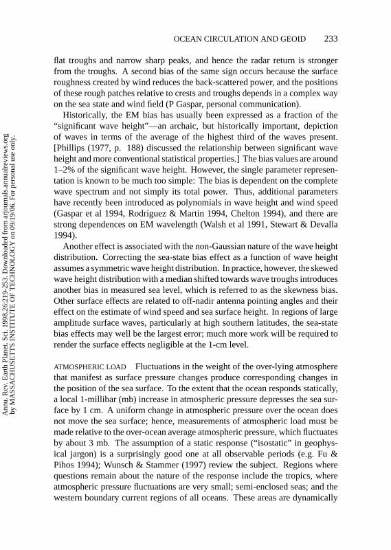
ATMOSPHERIC LOAD Fluctuations in the weight of the over-lying atmospherethat manifest as surface pressure changes produce corresponding changes inthe position of the sea surface. To the extent that the ocean responds statically,a local 1-millibar (mb) increase in atmospheric pressure depresses the sea sur-face by 1 cm. A uniform change in atmospheric pressure over the ocean doesnot move the sea surface; hence, measurements of atmospheric load must bemade relative to the over-ocean average atmospheric pressure, which fluctuatesby about 3 mb. The assumption of a static response (“isostatic” in geophys-ical jargon) is a surprisingly good one at all observable periods (e.g. Fu &Pihos 1994); Wunsch & Stammer (1997) review the subject. Regions wherequestions remain about the nature of the response include the tropics, whereatmospheric pressure fluctuations are very small; semi-enclosed seas; and thewestern boundary current regions of all oceans. These areas are dynamically
Ann
u. R
ev. E
arth
Pla
net.
Sci.
1998
.26:
219-
253.
Dow
nloa
ded
from
arj
ourn
als.
annu
alre
view
s.or
gby
MA
SSA
CH
USE
TT
S IN
STIT
UT
E O
F T
EC
HN
OL
OG
Y o
n 09
/19/
06. F
or p
erso
nal u
se o
nly.

P1: NBL/dat P2: NBL/ARY QC: NBL/BS T1: NBL
March 25, 1998 10:35 Annual Reviews AR055-08
234 WUNSCH & STAMMER
distinct from the oceanic interior, but the signal-to-noise ratios are also poorthere—and may well account for the apparent deviations from static response.Some uncertainty remains concerning the oceanic response at periods shorterthan about 10 days, but the variance is small.
POLAR MOTION Wobble of the rotation axis of the Earth [including the 14-month free (Chandler) wobble and the forced annual component] introduces atime-dependent centrifugal term into the apparent gravity seen by any observerfixed to the surface of the Earth (Wahr 1988). With present accuracies, theequivalent sea level change of order 2 cm is significant, and thus polar motionis determined and included as a correction.
SAMPLING AND ALIASING The fundamental sampling interval for TOPEX/POSEIDON is 10 days—the return time to any fixed location. Classical sam-pling theory (e.g. Bracewell 1978) shows that time-dependent motions occur-ring at periods shorter than 20 days will alias to longer periods. As an example,the 12.42-h principal lunar tide, M2, appears in a Fourier transform of the dataat a fixed location with an apparent period of 62 days. The choice of TOPEX/POSEIDON orbit was in large measure dictated by the need to prevent aliasingof tidal frequencies into important lower frequencies such as zero (the timeaverage) or the seasonal frequency—aliases that would have effectively pre-cluded study of important oceanographic phenomena (see discussion by Parkeet al 1987).
Oceanic variability occurs at all periods, from seconds to millions or billionsof years. The extent of the occurrence of energetically significant aliasing ofthe periods shorter than 20 days into apparent low-frequency variability in theTOPEX/POSEIDON data is a complex issue because of the very great regionaldifferences in the amplitudes and space/time scales of oceanic variability. Sim-ple spatial filtering can much reduce the aliasing, and in common with manygeophysical processes, the sea surface variability tends to have a “red” spec-trum. For such a spectrum, the rapid decay of energy with frequency rendersthe measurements comparatively immune to aliasing, with the tides as a no-table exception. The problem is exacerbated, however, by the dependence of theocean circulation on the spatial derivatives of the elevation rather than on theelevation itself—as the frequency spectrum of sea surface slope is much lessred than that for elevation. A full discussion is not yet available, but aspectsare described by Salby (1982), Wunsch (1989), Chelton & Schlax (1994), andGreenslade et al (1997). Eventually, a more complete description will becomenecessary.
The ability to sample the ocean adequately to avoid significant temporalaliasing must be distinguished from the related but different ability to produce
Ann
u. R
ev. E
arth
Pla
net.
Sci.
1998
.26:
219-
253.
Dow
nloa
ded
from
arj
ourn
als.
annu
alre
view
s.or
gby
MA
SSA
CH
USE
TT
S IN
STIT
UT
E O
F T
EC
HN
OL
OG
Y o
n 09
/19/
06. F
or p
erso
nal u
se o
nly.

P1: NBL/dat P2: NBL/ARY QC: NBL/BS T1: NBL
March 25, 1998 10:35 Annual Reviews AR055-08
OCEAN CIRCULATION AND GEOID 235
uniformly accurate physical-space maps of sea surface topography. Generallyspeaking, by using spatial filtering, the 10-day repeat orbit of TOPEX/POSEIDON is adequate to reduce serious aliasing from high-frequency non-tidal motions at the measurement positions. But because of the “diamondpattern” formed by the ground tracks in Figure 4, the sampling is inadequatefor production of accurate maps of short spatial scales of elevation associatedwith eddies in the interiors of the diamonds (the short spatial scales, whichare adequately sampled along track, cannot be extrapolated to the unsampledregions, but the long wavelengths can be usefully mapped). Temporal cover-age does remain an issue in some regions of rapid change, such as near themeandering Gulf Stream (see Minster & Gennero 1995) and in some tropicalregions. Should uniform high wavenumber mapping be required everywhereon the sea surface, then the only remedy is to fly additional altimeters; by goodfortune, coverage may be adequate in the next few years to permit such mapping(Greenslade et al 1997).
THE TIME-VARIABLE CIRCULATION
Figure 6a shows the time-averaged sea surface from four years (October 12,1992, to October 9, 1996) of TOPEX/POSEIDON data relative to the EGM96geoid, spatially filtered to remove any oceanic spatial structures with wave-lengths shorter than about 500 km. Such a surface contains any residual geoiderrors, including errors in the spherical harmonic expansion coefficients, aswell as errors of omission from coefficients simply set to zero (everythingabove spherical harmonic degree 360). Beginning with the earliest altimetricmissions, it was recognized that the time-dependent ocean variability could bedetermined independently of errors inN. One either forms a time-mean ¯η(θ, λ),
and works with anomalies1η = η − η or, less commonly, with the discretetime-derivativedη = [η(θ, λ, t +1t)− η(θ, λ, t)]/1t. In either case,N nolonger appears. (But at second order, errors inN affect the orbit determinationand can introduce spurious time variability into the measurement.) The ease ofthis removal of geoid error has led to a large literature on the time variabilityof the ocean circulation as seen at the sea surface. Figure 6b shows, for ex-ample, the spatially smoothed anomaly in one 10-day period of the flow fieldrelative to its four-year average.
Because of the novelty of the instrument, many papers have demonstrated bydirect comparison with more conventional instruments that the measurementswere accurate and believable. Thus, there are comparisons with, for exam-ple, tide gauges (Mitchum 1994), inverted echo sounders (Hallock et al 1995),current meters (Strub et al 1997, Wunsch 1997), atmospheric forcing clima-tologies (Chambers et al 1997, Stammer 1997b), and expendable temperature
Ann
u. R
ev. E
arth
Pla
net.
Sci.
1998
.26:
219-
253.
Dow
nloa
ded
from
arj
ourn
als.
annu
alre
view
s.or
gby
MA
SSA
CH
USE
TT
S IN
STIT
UT
E O
F T
EC
HN
OL
OG
Y o
n 09
/19/
06. F
or p
erso
nal u
se o
nly.

P1: NBL/dat P2: NBL/ARY QC: NBL/BS T1: NBL
March 25, 1998 10:35 Annual Reviews AR055-08
236 WUNSCH & STAMMER
measuring devices (XBTs; White & Tai 1995). There is no evidence for anyinconsistency beyond known error estimates and sampling disparities betweenin situ and altimetric measurements of the variability on time scales betweendays and years. (Global mean sea level has been a troubling exception; seeNerem et al 1997.)
The current meter data, in particular, have been used (Wunsch 1997) to un-derstand the vertical partitioning of the motions in the context of compensationin the vertical. Although the results are complicated in detail, and the coverageby current meters less than global, it appears that the sea level slope energyseen by the altimeter in low and middle latitudes is dominated by motionsin which there is first-order movement (compensation) by the interior densityfield. Thus, qualitatively, the altimeter primarily reflects movement of the deepisopycnals (surfaces of constant density) and only secondarily that of motionsextending unattenuated to the seafloor. High-latitude variability (poleward ofabout 40) appears more barotropic (uncompensated) owing to the weaker strat-ification and large values of|φ| in Equation 6; very strong seasonal changes inthe stratification also occur there.
Because of the dominant oceanographic paradigm of an unchanging generalcirculation, the novelty of being able to demonstrate oceanographic variabilityhas produced a very large literature, too large to review here, that displays thedegree of temporal variability in an immense variety of physical settings.Thegreatest importance of TOPEX/POSEIDON has been its vivid demonstrationthat the ocean is a global-scale fluid constantly evolving on all time and spacescales. Special attention has been paid to high-energy regions such as thewestern boundary currents, the Antarctic Circumpolar Current, interior fronts,regions of strong topographic gradients, and the Mediterranean Sea, but forreasons of space, we omit specific discussion of the results.
The Annual CycleThe seasonal cycle in the ocean is an important element in climate. Generallyspeaking, the oceanic response is the sum of a strong local effect (direct heatand moisture exchange with the atmosphere) plus a dynamical response fromremote disturbances, believed to be primarily wind-related (Gill & Niiler 1973).TOPEX/POSEIDON measurements directly display the very large-scale ther-mal response (e.g. White & Tai 1995, Chambers et al 1997, Stammer 1997b)plus dramatic propagating structures. Figure 7 shows the amplitude and phaseof the annual cycle of sea level. The very large amplitudes in the Kuroshioand Gulf Stream reflect the regions of intense wintertime air-sea exchange ofheat there. Although the northern and southern hemispheres are approximately180 out of phase, the ocean displays a complex spatial structure in its responseto annual forcing. Among a host of features, note that the northern-hemisphere
Ann
u. R
ev. E
arth
Pla
net.
Sci.
1998
.26:
219-
253.
Dow
nloa
ded
from
arj
ourn
als.
annu
alre
view
s.or
gby
MA
SSA
CH
USE
TT
S IN
STIT
UT
E O
F T
EC
HN
OL
OG
Y o
n 09
/19/
06. F
or p
erso
nal u
se o
nly.

P1: NBL/dat P2: NBL/ARY QC: NBL/BS T1: NBL
March 25, 1998 10:35 Annual Reviews AR055-08
OCEAN CIRCULATION AND GEOID 237
ocean generally has a larger amplitude than the southern. It is apparent in thealtimeter data that the annual cycle in the ocean shows very large variationsfrom year to year and is not a simple periodic phenomenon.
Second Order Moments (Including Spectra and RossbyWave Discussion)Although the altimeter is extremely useful in regional studies, its great noveltyis the ability to depict the global ocean. Several representations are required tofully understand the implications of the data. Letη′ = η−〈η〉, where the bracketdenotes the four-year average elevation; then Figure 8a depicts the great spatialvariability of〈η′2〉, and Figure 8b that of the slope variance(g/2Ä)2 〈(∂η′/∂s)2〉,with the bracket denoting a time average. The mean square ofη′ over four yearsis about 97 cm2, for an rms variability of less than 10 cm—which makes clearthe need for the elaborate error reduction procedure. The slope variance isrelated to the surface kinetic energy variance,KE, through
KE = g2
(2Ä sinφ)2
⟨(∂η′
∂s
)2⟩. (9)
Equation 9 represents the component of kinetic energy from the cross-trackgeostrophic velocity multiplied by 2 under the assumption of local isotropy(Stammer 1997a). These variances can be broken up into their contributionsby frequency band and (approximately only) by wavenumber band (Wunsch &Stammer 1995).
Figure 10 depicts the complex way in which the kinetic energy, as computedin Equation 9, shows an annual variability. These results display a spatialintricacy (e.g. in the high-latitude North Atlantic and the tropics) for whichonly the smallest beginnings of an explanation have as yet been attempted(White & Heywood 1995, Stammer & B¨oning 1996).
FREQUENCY/WAVENUMBER DEPICTION In view of the strong spatial inhomo-geneities visible in Figures 7–9, as well as the complex geometry of the oceanboundaries, a conventional frequency/wavenumber representation of the globaloceanic low-frequency variability is not the complete description that it wouldbe in a (Gaussian) spatially and temporally homogeneous field. Nonethe-less, the description remains useful and important. Figure 10 displays thefrequency/wavenumber power spectrum as computed by Wunsch & Stammer(1995), but now recomputed from four years of data rather than the two yearsavailable at that time. Until TOPEX/POSEIDON was flown, many of the space/time scales in these figures were simply unmeasurable by any known means.Apart from the quantitative description that is now available, a major conclusiondrawn from Figure 10 and other estimates is that the ocean varies on all space
Ann
u. R
ev. E
arth
Pla
net.
Sci.
1998
.26:
219-
253.
Dow
nloa
ded
from
arj
ourn
als.
annu
alre
view
s.or
gby
MA
SSA
CH
USE
TT
S IN
STIT
UT
E O
F T
EC
HN
OL
OG
Y o
n 09
/19/
06. F
or p
erso
nal u
se o
nly.

P1: NBL/dat P2: NBL/ARY QC: NBL/BS T1: NBL
March 25, 1998 10:35 Annual Reviews AR055-08
238 WUNSCH & STAMMER
Figure 10 (a) Frequency/wavenumber energy spectrum computed from a spherical harmonic fit,as described by Wunsch & Stammer (1995), but from four years of data vs two. Wavenumbersare actually in terms of spherical harmonic ordern, for which the wavelengths are approximately40,000 km/n. The total power integrates to 41 cm2 and contains no energy on spatial scales shorterthan about 400-km wavelength. The major low-frequency feature is the annual cycle, which isbroadband in wavenumber space. A small ridge near 60-day period has an rms amplitude of about0.9 cm and represents the residual uncorrected M2 and S2 semidiurnal tidal constituents, whichalias to this period. Much of this small residual is the surface manifestation of internal tides and isnot predictable. These unpredictable tidal elements may continue to require that future altimetricmissions fly in TOPEX/POSEIDON-like orbits to prevent the temporal aliases that are a featureof the Sun-synchronous orbits used for cheaper missions. (b) Frequency power density spectrumobtained froma by summing over all spherical harmonics. The annual, semi-annual, and 60-daytidal alias peaks are conspicuous. Some of the semi-annual peak is probably residual aliasingof diurnal tides. (c) Wavenumber power density spectrum, computed froma by summing overall frequencies and then converting (Wunsch & Stammer 1995) to the along-track great circlewavenumber spectrum of an equivalent homogeneous, isotropic process. Some high wavenumbershave been omitted because of the spatial filtering implicit in producinga.
Ann
u. R
ev. E
arth
Pla
net.
Sci.
1998
.26:
219-
253.
Dow
nloa
ded
from
arj
ourn
als.
annu
alre
view
s.or
gby
MA
SSA
CH
USE
TT
S IN
STIT
UT
E O
F T
EC
HN
OL
OG
Y o
n 09
/19/
06. F
or p
erso
nal u
se o
nly.
P1: NBL/dat P2: NBL/ARY QC: NBL/BS T1: NBL
March 25, 1998 10:35 Annual Reviews AR055-08
OCEAN CIRCULATION AND GEOID 239
and time scales; there are no spectral gaps, and there is no reason to believe thatany element of the circulation is strictly steady.
The MesoscaleOceanic kinetic energy (Figures 8b, 9) is dominated by the so-called mesoscale,which lies very roughly on spatial scales of 30–1000 km, with time scales of10–150 days. (There is no generally agreed upon definition; the motions corre-spond dynamically to the atmospheric “synoptic scale”—the weather systems.)Reviews of this subject can be found in Wunsch (1981b), Robinson (1983), andHolloway (1986b).
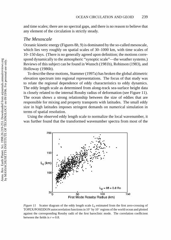
To describe these motions, Stammer (1997a) has broken the global altimetricelevation spectrum into regional representations. The focus of that study wasto relate the regional dependence of eddy characteristics to eddy dynamics.The eddy length scale as determined from along-track sea-surface height datais closely related to the internal Rossby radius of deformation (see Figure 11).The ocean shows a strong relationship between the size of eddies that areresponsible for mixing and property transports with latitudes. The small eddysize in high latitudes imposes stringent demands on numerical simulation interms of spatial resolution.
Using the observed eddy length scale to normalize the local wavenumber, itwas further found that the transformed wavenumber spectra from most of the
Figure 11 Scatter diagram of the eddy length scaleL0 estimated from the first zero-crossing ofTOPEX/POSEIDON autocorrelation functions in 10 by 10 regions of the world ocean and plottedagainst the corresponding Rossby radii of the first baroclinic mode. The correlation coefficientbetween the fields isr= 0.8.
Ann
u. R
ev. E
arth
Pla
net.
Sci.
1998
.26:
219-
253.
Dow
nloa
ded
from
arj
ourn
als.
annu
alre
view
s.or
gby
MA
SSA
CH
USE
TT
S IN
STIT
UT
E O
F T
EC
HN
OL
OG
Y o
n 09
/19/
06. F
or p
erso
nal u
se o
nly.

P1: NBL/dat P2: NBL/ARY QC: NBL/BS T1: NBL
March 25, 1998 10:35 Annual Reviews AR055-08
240 WUNSCH & STAMMER
world ocean—upon normalization by the local variance—are consistent witheach other in shape. An approximate universal rule for the energy distributionas a function of wavenumber can be written as
00(k) = 135k−0.7, 0.18≤ k ≤ 1.006,
135k−2.8, 1.006≤ k ≤ 2.057,
501k−4.6, 2.057≤ k ≤ 4.54.
(10)
Herek = k/k0, wherek0 is the wavenumber of the dominant local eddy scale.Other representations are possible too (Wunsch & Stammer 1995, Stammer1997a). Although the power laws in Equation 10 bear an intriguing resem-blance to the ones predicted by theories of geostraphic turbulance, there remainmajor theoretical issues in understanding the dynamical significance of thesedescriptions in terms of wave and turbulent interactions.
Rossby Wave ContributionsThe theoretical linear response of the ocean to atmospheric forcing at the periodswe are discussing is primarily in terms of so-called Rossby and topographicRossby waves plus the Kelvin wave, which is boundary or equatorially trapped.In idealized form, the waves exist as both “barotropic” (extending to the sea-floor unchanged) and “baroclinic” (compensated at a fixed intermediate depth;see Gill 1982). Because these waves have important dynamical consequences,and are a complete set for spectral representation, there have been a numberof attempts to demonstrate their existence in altimetric variability. Because ofthe completeness, the waves can represent arbitrary motions, whether linear ornot, in a topographically complex ocean with mean flows, and consequentlythe representation is of interest only if a very small number of waves canaccurately describe the ocean over large geographical areas. That is, one seeksto understand the extent to which expressions like Equation 10 are composedprimarily of linear wave-like phenomena or nonlinear “turbulent” ones. Alinear ocean is much easier to understand than a nonlinear one, and hence thedynamical distinction is important.
Attempts to find barotropic elements have tended to be inconclusive at best(Fu & Davidson 1995, Chechelnitsky 1996), except at high latitudes (see Fu& Smith 1996), presumably because barotropic modes in the altimeter recordare masked by the near-surface amplification of the baroclinic ones (Wunsch1997). Baroclinic motions have fast phase and group velocities in the tropicsrelative to mid-latitudes, which permits use in these regions of comparativelyshort records. Convincing demonstrations of important linear baroclinic waveresponse in the tropics have been provided by Boulanger & Menkes (1995),Boulanger & Fu (1996), and Jacobs et al (1994).
Ann
u. R
ev. E
arth
Pla
net.
Sci.
1998
.26:
219-
253.
Dow
nloa
ded
from
arj
ourn
als.
annu
alre
view
s.or
gby
MA
SSA
CH
USE
TT
S IN
STIT
UT
E O
F T
EC
HN
OL
OG
Y o
n 09
/19/
06. F
or p
erso
nal u
se o
nly.

P1: NBL/dat P2: NBL/ARY QC: NBL/BS T1: NBL
March 25, 1998 10:35 Annual Reviews AR055-08
OCEAN CIRCULATION AND GEOID 241
Chelton & Schlax (1996; see also Polito & Cornillon 1997) described theappearance of baroclinic Rossby waves at mid-latitudes in a band of frequenciesaround one half to two cycles per year. Cipollini et al (1997) show that in themid-latitude North Atlantic, the waves are strongly correlated with surfacetemperature anomalies. The most striking aspect of these results is that thewaves appear to have phase speeds systematically higher (up to a factor of two)than produced by the theory for linear free waves. Understanding whether thisanomaly is of dynamical significance, or whether it is a kinematic confusionof group and phase velocities in the presence of boundary reflections, forcing,and dissipation, is the subject of much current work (e.g. Killworth et al 1997,Qiu et al 1997). A quantitative estimate is not yet available of the fraction ofthe variability energy explicable by purely linear modes.
Jacobs & Mitchell (1996) have called attention to apparent low-frequencywave-like phenomena in the Southern Ocean [and described from non-altimetricdata by White & Peterson (1996)], proposing a coupling with the geographi-cally remote El Nino–Southern Oscillation in the ocean and atmosphere. Theevidence, while suggestive, is based on records scarcely longer than one cycle ofthe supposed phenomenon and is dependent upon the GEOSAT measurementsfor an extended record.
Eddy FluxesAn intense mesoscale eddy field in the ocean exists in mid-latitudes at periodsmuch too short to be described by linear baroclinic waves. The implied nonlin-earities show the possibility of significant eddy transports of momentum, heat,oxygen, and other chemical species. Before the advent of the altimeter data, theonly way to determine the importance of eddy properties was through the long,laborious, and expensive deployment of moored instruments at specific posi-tions in the ocean or through use of the erratic coverage by free drifters. Mostof the available estimates of eddy momentum flux from altimetry are still fromthe GEOSAT instrument (e.g. Wilkin & Morrow 1994), although Strub et al(1997) used TOPEX/POSEIDON data; these studies support suggestions thatnear major meandering current systems, such as the Gulf Stream and AntarcticCircumpolar Current, eddy momentum fluxes are very important.
Theories that relate eddy transport properties (temperature, salt) to the ther-modynamic mean state of a fluid were pioneered by Green (1970) for atmo-spheric conditions. These ideas, which are based on baroclinic instabilitymechanisms, have now been applied to the ocean (Visbeck et al 1997). Si-multaneously, the theory of geostrophic turbulence was extended to provideestimates of eddy transports of a tracer field, with the eddy transport parameter-ized in terms of the mean flow field (Holloway 1986a, Held & Larichev 1996).Stammer (1997c) recently used these ideas and the eddy scales calculated from
Ann
u. R
ev. E
arth
Pla
net.
Sci.
1998
.26:
219-
253.
Dow
nloa
ded
from
arj
ourn
als.
annu
alre
view
s.or
gby
MA
SSA
CH
USE
TT
S IN
STIT
UT
E O
F T
EC
HN
OL
OG
Y o
n 09
/19/
06. F
or p
erso
nal u
se o
nly.
P1: NBL/dat P2: NBL/ARY QC: NBL/BS T1: NBL
March 25, 1998 10:35 Annual Reviews AR055-08
242 WUNSCH & STAMMER
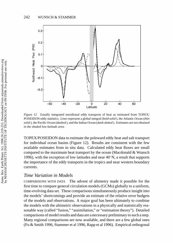
Figure 12 Zonally integrated meridional eddy transports of heat as estimated from TOPEX/POSEIDON eddy statistics.Linesrepresent a global integral (bold solid), the Atlantic Ocean (thinsolid), the Pacific Ocean (dashed), and the Indian Ocean (dash-dotted). Estimates are not obtainedin theshaded low-latitude area.
TOPEX/POSEIDON data to estimate the poleward eddy heat and salt transportfor individual ocean basins (Figure 12). Results are consistent with the fewavailable estimates from in situ data. Calculated eddy heat fluxes are smallcompared to the maximum heat transport by the ocean (Macdonald & Wunsch1996), with the exception of low latitudes and near 40N, a result that supportsthe importance of the eddy transports in the tropics and near western boundarycurrents.
Time Variation in ModelsCOMPARISONS WITH DATA The advent of altimetry made it possible for thefirst time to compare general circulation models (GCMs) globally to a uniform,time-evolving data set. These comparisons simultaneously produce insight intothe models’ shortcomings and provide an estimate of the relative error budgetsof the models and observations. A major goal has been ultimately to combinethe models with the altimetric observations in a physically and statistically rea-sonable way (called “fusion,” “assimilation,” or “estimation theory”). Detailedcomparisons of model results and data are a necessary preliminary to such a step.Many regional comparisons are now available, and there are a few global ones(Fu & Smith 1996, Stammer et al 1996, Rapp et al 1996). Empirical orthogonal
Ann
u. R
ev. E
arth
Pla
net.
Sci.
1998
.26:
219-
253.
Dow
nloa
ded
from
arj
ourn
als.
annu
alre
view
s.or
gby
MA
SSA
CH
USE
TT
S IN
STIT
UT
E O
F T
EC
HN
OL
OG
Y o
n 09
/19/
06. F
or p
erso
nal u
se o
nly.

Figure 6
Ann
u. R
ev. E
arth
Pla
net.
Sci.
1998
.26:
219-
253.
Dow
nloa
ded
from
arj
ourn
als.
annu
alre
view
s.or
gby
MA
SSA
CH
USE
TT
S IN
STIT
UT
E O
F T
EC
HN
OL
OG
Y o
n 09
/19/
06. F
or p
erso
nal u
se o
nly.

Figure 6 (a) Four-year average of the oceanic surface elevation, <η> = S − N, from TOPEX/POSEIDON data. Superimposed are the geostrophically computed velocity vec- tors implied by Equations 2 and 3; the near-equatorial and small values are omitted for clarity. Note that all structures with a spatial wavelength smaller than 500 km have been omitted because they would be dominated by geoid error. (b) Example of the anomaly of elevation η′ = η − <η>, relative to time mean <η> in (a) during one 10-day period (March 10−20, 1993). The geostrophic flow vectors corresponding to the elevation anomaly are superposed. Wavelengths shorter than about 500 km have again been omitted to permit some visual clarity. The actual anomaly field is far more complex and visually dominated by the omitted small scales. Figure 7 Amplitude (a) and phase (b) of the annual cycle of elevation in TOPEX/PO-SEIDON from four years of data. Amplitude is in centimeters, phase in degrees measured from January 1, 1993. Areas of extreme air/sea exchange produce large elevation changes as heat is added and removed by the atmosphere. The structures apparent in the quieter oceanic interior are related to wave-like motions. Note rough north/south phase shift by 180; the detailed structure in the phases particularly in the tropics and at high latitudes is apparent. (Next page) Figure 8 (a) Root mean square (rms) elevation anomaly <η> and (b) g2/(Ω)2<(∂η′/∂s)2> = (sin φ)2 •KE from four years of data. Units are in centimeters and (cm /s)2, respectively. The weighted kinetic energy is employed to avoid the equatorial singularity in the geo- strophic kinetic energy. The very great inhomogeneity in oceanic variability with space is apparent here, with the quietest areas showing variability of less than 2 cm in eleva- tion––close to the present noise level of the overall system.
Ann
u. R
ev. E
arth
Pla
net.
Sci.
1998
.26:
219-
253.
Dow
nloa
ded
from
arj
ourn
als.
annu
alre
view
s.or
gby
MA
SSA
CH
USE
TT
S IN
STIT
UT
E O
F T
EC
HN
OL
OG
Y o
n 09
/19/
06. F
or p
erso
nal u
se o
nly.

Figure 7
Ann
u. R
ev. E
arth
Pla
net.
Sci.
1998
.26:
219-
253.
Dow
nloa
ded
from
arj
ourn
als.
annu
alre
view
s.or
gby
MA
SSA
CH
USE
TT
S IN
STIT
UT
E O
F T
EC
HN
OL
OG
Y o
n 09
/19/
06. F
or p
erso
nal u
se o
nly.
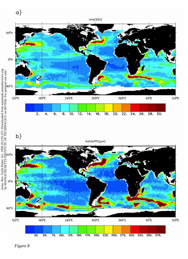
Figure 8
Ann
u. R
ev. E
arth
Pla
net.
Sci.
1998
.26:
219-
253.
Dow
nloa
ded
from
arj
ourn
als.
annu
alre
view
s.or
gby
MA
SSA
CH
USE
TT
S IN
STIT
UT
E O
F T
EC
HN
OL
OG
Y o
n 09
/19/
06. F
or p
erso
nal u
se o
nly.
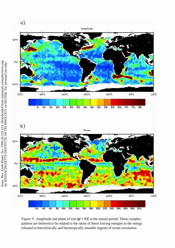
Figure 9 Amplitude and phase of (sin φ)2 • ΚΕ at the annual period. These complex patterns are believed to be related to the ratios of direct forcing energies to the energy released in baroclinically and barotropically unstable regions of ocean circulation.
Ann
u. R
ev. E
arth
Pla
net.
Sci.
1998
.26:
219-
253.
Dow
nloa
ded
from
arj
ourn
als.
annu
alre
view
s.or
gby
MA
SSA
CH
USE
TT
S IN
STIT
UT
E O
F T
EC
HN
OL
OG
Y o
n 09
/19/
06. F
or p
erso
nal u
se o
nly.

Figure 14
Ann
u. R
ev. E
arth
Pla
net.
Sci.
1998
.26:
219-
253.
Dow
nloa
ded
from
arj
ourn
als.
annu
alre
view
s.or
gby
MA
SSA
CH
USE
TT
S IN
STIT
UT
E O
F T
EC
HN
OL
OG
Y o
n 09
/19/
06. F
or p
erso
nal u
se o
nly.

Figure 14 Results from a global optimization of a GCM, surface forcing fields, and a year of TOPEX/POSEIDON data (from Stammer et al 1997). (a) Time–mean velocity es- timate v~ (cm/s) at 60-m depth, and the surface elevation η~ in centimeters. (b) Potential temperature θ~ (in degrees Centigrade) and flow vectors in centimeters per second (small flow vectors are omitted) at level 10 (610 m in the model). (c) Same as b, except at 2450 m (level 15). Figure 15 Changes required in the US National Center for Environmental Prediction (NCEP)-provided estimates in (a) the 10-day averaged freshwater flux field and (b) the heat flux as they emerge from the optimization for TOPEX/POSEIDON repeat cycle 21 (early September 1993). Contour intervals in a and b are 1 cm/year and 2 W m−2, respec- tively. These changes are acceptable within plausible guessed errors for the NCEP prod- uct and are required for consistency with the oceanographic measurements used to pro- duce the results in Figure 14.
Ann
u. R
ev. E
arth
Pla
net.
Sci.
1998
.26:
219-
253.
Dow
nloa
ded
from
arj
ourn
als.
annu
alre
view
s.or
gby
MA
SSA
CH
USE
TT
S IN
STIT
UT
E O
F T
EC
HN
OL
OG
Y o
n 09
/19/
06. F
or p
erso
nal u
se o
nly.

Figure 14
Ann
u. R
ev. E
arth
Pla
net.
Sci.
1998
.26:
219-
253.
Dow
nloa
ded
from
arj
ourn
als.
annu
alre
view
s.or
gby
MA
SSA
CH
USE
TT
S IN
STIT
UT
E O
F T
EC
HN
OL
OG
Y o
n 09
/19/
06. F
or p
erso
nal u
se o
nly.

P1: NBL/dat P2: NBL/ARY QC: NBL/BS T1: NBL
March 25, 1998 10:35 Annual Reviews AR055-08
OCEAN CIRCULATION AND GEOID 243
functions (EOFs), spectra, and spatial variability have all been used as descrip-tive tools. A summary would be that, even in the highest resolution models sofar, there are both quantitative and qualitative disparities, manifested primarilyas a failure of the models to display adequate variability on any time or lengthscale. We suspect, but cannot prove, that the low energies are largely a resultof a failure to achieve adequate spatial resolution, which is probably less than5 km at mid-latitudes, and to reduce the associated numerical friction. If theobserved low-frequency/low-wavenumber variability is the result of scale cou-pling in the fluid, either kinematic or dynamic (turbulent cascades), coarse res-olution models without observational constraints will systematically underpre-dict oceanic variability on all scales and, in particular, will underestimate eddytransports.
COMBINING DATA WITH MODELS: THE ESTIMATION PROBLEM Numerical mod-els can be regarded as a summary of our imperfect knowledge of the oceancirculation as reflected in the equations of motion and the known boundary andinitial conditions. Observations are another repository of information about thecirculation: information that is incomplete and noisy in different ways frommodels. The estimation problem seeks to combine the two types of informationinto a single best-estimate of the ocean circulation.
A great deal is known of the generic model/data problem, and entire text-books (Bennett 1992, Wunsch 1996) as well as hundreds of papers and meetingreports (e.g. Malanotte-Rizzoli 1996) exist on the problem in oceanographyalone, not to speak of the immense general literature on estimation theory. Asdescribed by Wunsch (1996), in numerical practice, most systematic approachesto the problem reduce to the equivalent of a least-squares analysis minimizingthe mean-square difference of the model output and the observations, suitablyweighted by the error covariance matrices of the data and of the model. Ad-justable or determinable parameters include the surface forcing (wind-stressand buoyancy fluxes), initial conditions, and model parameters such as frictioncoefficients. In nonglobal models, inflows through open sidewalls can be in-cluded as control parameters. Several different algorithms have been employedfor numerical minimization. Many of these algorithms fall into the generalclassifications of sequential (filters and smoothers), iterative (adjoint or Pon-tryagin Principle), and Monte Carlo, and all have their adherents; the readeris referred to the literature for details. Here we will state only that the majorpractical difficulties can be understood as (a) the very large problem dimensionfor global scale estimation, (b) model nonlinearity, and (c) inability to properlyspecify model error covariances.
Most efforts have been devoted to regional scales, using simple ad hocschemes with a focus on mapping the oceanic mesoscale. In these studies, thequestion of the correct weighting of model and data is ignored, and the model
Ann
u. R
ev. E
arth
Pla
net.
Sci.
1998
.26:
219-
253.
Dow
nloa
ded
from
arj
ourn
als.
annu
alre
view
s.or
gby
MA
SSA
CH
USE
TT
S IN
STIT
UT
E O
F T
EC
HN
OL
OG
Y o
n 09
/19/
06. F
or p
erso
nal u
se o
nly.

P1: NBL/dat P2: NBL/ARY QC: NBL/BS T1: NBL
March 25, 1998 10:35 Annual Reviews AR055-08
244 WUNSCH & STAMMER
is “nudged” toward the data through weights chosen subjectively or from sim-plified physical assumptions. Recently, more generally useful methods havecome into use [e.g. Morrow & De Mey (1995), who use a Lagrange multiplierformulation (adjoint method) of least-squares]. For adequate mapping of themesoscale by altimetry, multiple simultaneous missions are required; althoughthis confluence of missions may soon occur, mesoscale mapping at the presenttime represents an extreme use of the data, and we do not pursue it here.
A demonstration of a systematic approach to the basin-scale problem wasdescribed by Stammer & Wunsch (1996). A general circulation model wasformally linearized by numerically perturbing it in a sequence of regions anddepths; the resulting Green’s functions were employed as a new linear modelto represent the differences between the TOPEX/POSEIDON observations andthe forecast of those observations by the nonlinear model. [Great advantagesexist if linear estimation theory can be used rather than nonlinear methods. Theapparent success of the linearization for many ocean circulation problems con-trasts with the meteorological experience (e.g. Daley 1991).] The estimationproblem was then solved in terms of perturbations to the initial and boundarysystem conditions, with the full oceanic-state estimate as the original GCMvalues plus the linearized estimation values. A similar, but more elaborate,calculation also using tomographic data was carried out by Menemenlis et al(1997) for the Mediterranean Sea and by the Acoustic Thermometry of OceanClimate (ATOC) Consortium (paper in preparation) for the entire North PacificOcean. This subject is in its infancy, but it is rapidly emerging as a majorbranch of ocean circulation studies and will likely dominate the observationaldiscussion in the future.
THE ABSOLUTE AND TIME-INDEPENDENTCIRCULATIONS
The absolute circulation is defined from the instantaneous values of veloc-ity, temperature, salinity, and other state variables. The separation into time-average and temporal anomaly is often useful, but it can also be artificial andconfusing for several reasons. Because the spectra displayed above show noevidence for any low-frequency cut-off in oceanic variability, the time-averagedvalue can be an accident of the averaging interval. Furthermore, becausethe ocean circulation is a fluid flow governed by a nonlinear vector field the-ory, one cannot separate the dynamics into distinct time-dependent and time-independent components; the time-dependent flow generates mean or rectifiedflows, which are part of the time average. For this reason, it is better to speakof the absolute circulation at a fixed timet, whose average might be calculatedand interpreted. Employing altimetry in this way requires an accurate geoid.
Ann
u. R
ev. E
arth
Pla
net.
Sci.
1998
.26:
219-
253.
Dow
nloa
ded
from
arj
ourn
als.
annu
alre
view
s.or
gby
MA
SSA
CH
USE
TT
S IN
STIT
UT
E O
F T
EC
HN
OL
OG
Y o
n 09
/19/
06. F
or p
erso
nal u
se o
nly.

P1: NBL/dat P2: NBL/ARY QC: NBL/BS T1: NBL
March 25, 1998 10:35 Annual Reviews AR055-08
OCEAN CIRCULATION AND GEOID 245
The Geoid ProblemThe spatial variations inN relative to the reference ellipsoidE approach 100 m.N(0) is any geoid (height) estimate made wholly independent of altimetry.Such geoids—deduced from spacecraft tracking, marine and land gravity mea-surements, etc—have errors exceeding 10 m. The magnitude ofη is no morethan 1 or 2 m; thus,N(1) ≡ 〈S〉 is an improved geoid. The approximation isadequate for many geophysical and military purposes and was used to justifythe launch of GEOSAT.
Any information about the ocean circulation leads to an estimate of ¯η and afurther improved estimate of
N(2) = N(1)− η. (11)
Thus, there is a long and continuing symbiosis between altimetric measurementsof circulation and the problems of depicting and understanding the Earth’sgravity field. This relationship is of ever-growing importance, as efforts areunderway to radically improve estimates of the marine geoid through dedicatedspacecraft (e.g. Ganachaud et al 1997 and the references therein). In someregional studies (e.g. Porter et al 1996), the geoid height estimateN(2) hasbeen labeled a “synthetic” geoid. The terminology is misleading, as such anestimate is no more synthetic than any other. [Because there are correlations ofbottom topography with the geoid (e.g. Watts et al 1985), high spatial resolutionaltimetry can be used to reconstruct much of the seafloor structure; see Hwang& Parsons (1995) for an example. In principle, the process could be reversedso that knowledge of the seafloor topography and of the underlying tectonicswould be used to construct an accurate geoid. This procedure does not seem tohave been pursued systematically, however, and in general, because of altimetricmeasurements, the geoid is now better known than the seafloor topography overmuch of the oceans.]
The computation in Equation 11 does not help the physical oceanographer.Despite the progress made in the past 20 years in geoid estimation, we mustreturn to the problem described by Wunsch & Gaposchkin (1980): whether theindependent information available inN(0), S, andη can be used to simultane-ously estimate all three fields—thus improving knowledge of the absolute oceancirculation and of the geoid. [The interaction of physical oceanography andgeodesy has a long and not always illuminating history—see Sturges (1974),Balazs & Douglas (1979).]
The initial point of departure for a discussion of the marine geoid thus has to bean analysis of the existing accuracy with which the oceanic general circulationis understood and its manifestation as a sea surface slope. This discussion isin turn best divided into results dependent upon conventional oceanographicanalyses and those derived from GCMs.
Ann
u. R
ev. E
arth
Pla
net.
Sci.
1998
.26:
219-
253.
Dow
nloa
ded
from
arj
ourn
als.
annu
alre
view
s.or
gby
MA
SSA
CH
USE
TT
S IN
STIT
UT
E O
F T
EC
HN
OL
OG
Y o
n 09
/19/
06. F
or p
erso
nal u
se o
nly.
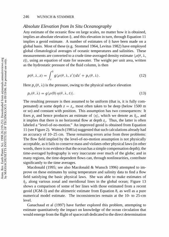
P1: NBL/dat P2: NBL/ARY QC: NBL/BS T1: NBL
March 25, 1998 10:35 Annual Reviews AR055-08
246 WUNSCH & STAMMER
Absolute Elevation from In Situ OceanographyAny estimate of the oceanic flow on large scales, no matter how it is obtained,implies an absolute elevation ˜η, and this elevation in turn, through Equation 11implies a geoid estimate. A number of estimates of ˜η have been made on aglobal basis. Most of these (e.g. Stommel 1964, Levitus 1982) have employedglobal climatological averages of oceanic temperatures and salinities. Thesemeasurements are converted to a crude time-averaged density estimate〈ρ(θ , λ,z)〉, using an equation of state for seawater. The weight per unit area, writtenas the hydrostatic pressure of the fluid column, is then
p(θ, λ, z) =∫ 0
zg〈ρ(θ, λ, z′)〉dz′ + ps(θ, λ) . (12)
Hereps(θ , λ) is the pressure, owing to the physical surface elevation
ps(θ, λ) = g〈ρ(0) η(θ, λ, t)〉. (13)
The resulting pressure is then assumed to be uniform (that is, it is fully com-pensated) at some depthz= zc, most often taken to be deep (below 1500 mor so) and constant with position. This assumption has two consequences: Itfixes ps and hence produces an estimate of〈η〉, which we denote as ˜ηρ , andit implies that there is no horizontal flow at depthzc. Thus, the latter is oftenlabeled a “level-of-no-motion.” An improved geoid is obtained from Equation11 (see Figure 2). Wunsch (1981a) suggested that such calculations already hadan accuracy of 10–25 cm. These remaining errors arise from three problems:The flow field implied by the level-of-no-motion assumption is not physicallyacceptable, as it fails to conserve mass and violates other physical laws (in otherwords, there is no evidence that the ocean has a simple compensation depth); thetime-averaged hydrography is very inaccurate over much of the globe; and inmany regions, the time-dependent flows can, through nonlinearities, contributesignificantly to the time averages.
Macdonald (1995; see also Macdonald & Wunsch 1996) attempted to im-prove on these estimates by using temperature and salinity data to find a flowfield satisfying the basic physical laws. She was able to make estimates ofηρ along various zonal and meridional lines in the global ocean; Figure 13shows a comparison of some of her lines with those estimated from a recentgeoid (JGM-3) and the altimetric estimate from Equation 8, as well as a purenumerical model estimate. The inconsistencies remain at the 10- to 25-cmlevel.
Ganachaud et al (1997) have further explored this problem, attempting toestimate quantitatively the impact on knowledge of the ocean circulation thatwould emerge from the flight of spacecraft dedicated to the direct determination
Ann
u. R
ev. E
arth
Pla
net.
Sci.
1998
.26:
219-
253.
Dow
nloa
ded
from
arj
ourn
als.
annu
alre
view
s.or
gby
MA
SSA
CH
USE
TT
S IN
STIT
UT
E O
F T
EC
HN
OL
OG
Y o
n 09
/19/
06. F
or p
erso
nal u
se o
nly.

P1: NBL/dat P2: NBL/ARY QC: NBL/BS T1: NBL
March 25, 1998 10:35 Annual Reviews AR055-08
OCEAN CIRCULATION AND GEOID 247
Figure 13 Comparison ofη from TOPEX/POSEIDON data and the so-called JGM-3 geoid (Tapleyet al 1997;dashed lines) with those from a hydrographic inversion (Macdonald 1995;solid lines),and with a global oceanic general circulation model (Stammer et al 1996;dash-dot lines) alongseveral zonal lines in the Pacific Ocean (latitudes 47N, 24N, etc). Agreement is generally at the10-cm level or better, but the discrepancies are oceanographically of first-order importance.
of N. The discussion is a complicated one, involving production of error co-variance matrices forN derived from hypothetical missions, as compared withthose from estimates of ˜ηρ . A summary conclusion is that major improvementsin the ocean circulation could be obtained if missions can meet very demandingdesign specifications.
Absolute Altimetry in ModelsAs with the temporal anomalies, the best use of altimetry is in combinationwith an accurate general circulation model. Conceptually, the use of absolutealtimetry is identical to the temporal anomaly data: minimization of an objectivefunction that represents the weighted mean square difference between the modeloutput and the observations. If the absolute altimetry is to be employed with a
Ann
u. R
ev. E
arth
Pla
net.
Sci.
1998
.26:
219-
253.
Dow
nloa
ded
from
arj
ourn
als.
annu
alre
view
s.or
gby
MA
SSA
CH
USE
TT
S IN
STIT
UT
E O
F T
EC
HN
OL
OG
Y o
n 09
/19/
06. F
or p
erso
nal u
se o
nly.
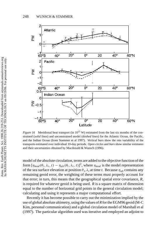
P1: NBL/dat P2: NBL/ARY QC: NBL/BS T1: NBL
March 25, 1998 10:35 Annual Reviews AR055-08
248 WUNSCH & STAMMER
Figure 16 Meridional heat transport (in 1015 W) estimated from the last six months of the con-strained (solid lines) and unconstrained model (dashed lines) for the Atlantic Ocean, the Pacific,and the Indian Ocean (from Stammer et al 1997).Vertical barsshow the rms variability of thetransports estimated over individual 10-day periods.Open circlesandbarsshow similar estimatesand their uncertainties obtained by Macdonald & Wunsch (1996).
model of the absolute circulation, terms are added to the objective function of theform [ηmod(θi , λi , t)− ηalt (θi , λi , t)]
2, whereηmod is the model representationof the sea surface elevation at positionθ i, λi at timet. Becauseηalt contains anyremaining geoid error, the weighting of these terms must properly account forthat error; in turn, this means that the geographical spatial error covariance,R,is required for whatever geoid is being used.R is a square matrix of dimensionequal to the number of horizontal grid points in the general circulation model;calculating and using it represents a major computational effort.
Recently it has become possible to carry out the minimization implied by theuse of global absolute altimetry, using the values ofRfor the EGM96 geoid (M-CKim, personal communication) and a global circulation model of Marshall et al(1997). The particular algorithm used was iterative and employed an adjoint to
Ann
u. R
ev. E
arth
Pla
net.
Sci.
1998
.26:
219-
253.
Dow
nloa
ded
from
arj
ourn
als.
annu
alre
view
s.or
gby
MA
SSA
CH
USE
TT
S IN
STIT
UT
E O
F T
EC
HN
OL
OG
Y o
n 09
/19/
06. F
or p
erso
nal u
se o
nly.

P1: NBL/dat P2: NBL/ARY QC: NBL/BS T1: NBL
March 25, 1998 10:35 Annual Reviews AR055-08
OCEAN CIRCULATION AND GEOID 249
the original model; the adjoint was generated using a special compiler (Giering& Kaminski 1997) that operates on the forward model code. Although thus farrestricted by computer limitations to 2 of horizontal resolution (the numberof model grid points is 180 by 80 horizontally by 21 vertically), it is possibleto produce estimates of the ocean circulation on a 10-day basis in such a waythat the model is consistent with the 10-day absolute surface topography, withtime-varying surface topography and with the known meteorological forcingand basic temperature and salinity data for the ocean (Stammer et al 1997).Figure 14 depicts the time–mean absolute velocity at 60, 610, and 2450 m;the corresponding absolute surface elevation (Figure 14a); and the temperaturefield during the year 1995 from a combined model/data optimization (compareto Figure 6a). Figure 15 shows, as an example of what is now possible, theestimated adjustment to the air-sea freshwater flux (Figure 15a) and heat flux(Figure 15b) required to render the model consistent with the observations.Figure 16 shows how the TOPEX/POSEIDON data modify the model estimateof the climatologically important meridional flux of heat. Results from thisform of model/data combination are not yet definitive, but they will become soover the next several years. The major issues are adequate computer power andthe need to more clearly formulate expressions of model error; data errors alsoremain inadequately known.
THE FUTURE
TOPEX/POSEIDON altimetry has demonstrated the first practical global ob-servation system for the oceanic general circulation. Remaining errors in thepresent system will gradually be reduced as understanding of the residual er-ror sources improves. The combination of TOPEX/POSEIDON data with thatfrom simultaneous missions of lower accuracy and precision (ERS-1 and 2 andGEOSAT-Follow-On) and more traditional in situ data will, over the next fewyears, provide a greatly improved estimate of oceanic variability on time scalesfrom a few days to a decade. As oceanic GCMs continue to improve, there willbe ever more accurate three-dimensional estimates of the absolute circulationon a frequent basis (perhaps weekly), with an emerging understanding on thelimits of oceanic forecast skill.
These things can all be expected with a considerable degree of confidencebecause they are dependent primarily upon data now in hand. The real un-certainty concerns the future of high-accuracy altimetric missions. Spacecraft,because of their great expense and public visibility, are flown in a political arenawhose wisdom is not easily predicted; furthermore, the vagaries of launch andon-board hardware and software failures render all such systems vulnerable topremature and catastrophic ends. At the present time, barring such failures,
Ann
u. R
ev. E
arth
Pla
net.
Sci.
1998
.26:
219-
253.
Dow
nloa
ded
from
arj
ourn
als.
annu
alre
view
s.or
gby
MA
SSA
CH
USE
TT
S IN
STIT
UT
E O
F T
EC
HN
OL
OG
Y o
n 09
/19/
06. F
or p
erso
nal u
se o
nly.

P1: NBL/dat P2: NBL/ARY QC: NBL/BS T1: NBL
March 25, 1998 10:35 Annual Reviews AR055-08
250 WUNSCH & STAMMER
satellite altimetry of the TOPEX/POSEIDON class appears assured for severalyears into the twenty-first century (current rubrics are Jason, ENVISAT, etc).As the data set grows, and our skill in interpreting it improves, we can antici-pate that study of the ocean circulation will finally become a true quantitativescience freed from the straitjacket of inadequate observation technology.
ACKNOWLEDGMENTS
P Gaspar, L-L Fu, D Chelton, and R Rapp provided many helpful comments.Supported in part by contracts from the National Aeronautics and Space Ad-ministration (NAG5-3724) and the Jet Propulsion Laboratory (958125).
Visit the Annual Reviews home pageathttp://www.AnnualReviews.org.
Literature Cited
Andersen OB, Woodworth PL, Flather RA.1995. Intercomparison of recent ocean tidemodels.J. Geophys. Res.100:25261–82
Balazs EI, Douglas BC. 1979. Geodetic level-ing and the sealevel slope along the Californiacoast.J. Geophys. Res.84:6195–6206
Bennett AF. 1992.Inverse Methods in Physi-cal Oceanography.Cambridge: CambridgeUniv. Press. 346 pp.
Boulanger J-P, Fu L-L. 1996. Evidence ofboundary reflection of Kelvin and first modeRossby waves from TOPEX/POSEIDON sealevel data.J. Geophys. Res.101:16361–71
Boulanger J-P, Menkes C. 1995. Propagationand reflection of long equatorial waves in thePacific Ocean during the 1992–1993 El Nino.J. Geophys. Res.100:25041–60
Bracewell RN. 1978.The Fourier Transformand Its Applications.New York: McGraw-Hill. 444 pp.
Chambers DP, Tapley BD, Stewart RH. 1997.Long-period ocean heat storage rates andbasin-scale heat fluxes from TOPEX.J. Geo-phys. Res.102:10525–33
Chechelnitsky M. 1996.Global barotropic vari-ability of the ocean in response to atmo-spheric forcing based on multichannel re-gression and Kalman filter techniques. MSthesis. Mass. Inst. Technol./Woods HoleOceanogr. Inst. Joint Program. 112 pp.
Chelton DB. 1988.WOCE/NASA Altimeter Al-gorithm Workshop. US WOCE Tech. Rep. 2.US Planning Off. World Ocean Circ. Exp.,Texas A & M Univ.,College Station, Texas.70 pp.
Chelton DB. 1995. The sea state bias in al-timeter estimates of sea level from colinear
analysis of TOPEX data.J. Geophys. Res.99:24995–5008
Chelton DB, Schlax MG. 1994. The resolutioncapability of an irregularly sampled dataset:with application to Geosat altimeter data.J.Atmos. Ocean Technol.11:534–50
Chelton DB, Schlax MG. 1996. Global obser-vations of oceanic Rossby waves.Science272:234–38
Cipollini P, Cromwell D, Jones MS, QuartlyGD, Challenor PG. 1997. Concurrent altime-ter and infrared observations of Rossby wavepropagation near 34N in the Northeast At-lantic.Geophys. Res. Lett.24:885–92
Daley R. 1991.Atmospheric Data Analysis.Cambridge: Cambridge Univ. Press. 457 pp.
Dietrich G, Kalle K, Krauss W, Siedler G.1975.General Oceanography, An Introduc-tion.Transl. S Roll, HU Roll. New York: Wi-ley. 626 pp. 2nd ed. (From German)
Douglas BC, Cheney RE. 1990. Geosat: Be-ginning a new era in satellite oceanography.J. Geophys. Res.95:2833–36
Douglas BC, McAdoo DC, Cheney RE. 1987.Oceanographic and geophysical applicationsof satellite altimetry.Rev. Geophys. (Suppl.US Natl. Rep. Int. Union Geod. Geophys.1983–1986)25:875–80
Fu L-L, Cheney RE. 1995. Application of satel-lite altimetry to ocean circulation studies:1987–1994.Rev. Geophys. (Suppl. US Natl.Rep. Int. Union Geod. Geophys., 1991–1994)32:213–23
Fu L-L, Christensen EJ, Yamarone CA, Lefeb-vre M, Menard Y, et al. 1994. TOPEX/POSEIDON mission overview.J. Geophys.Res.99:24369–82
Ann
u. R
ev. E
arth
Pla
net.
Sci.
1998
.26:
219-
253.
Dow
nloa
ded
from
arj
ourn
als.
annu
alre
view
s.or
gby
MA
SSA
CH
USE
TT
S IN
STIT
UT
E O
F T
EC
HN
OL
OG
Y o
n 09
/19/
06. F
or p
erso
nal u
se o
nly.

P1: NBL/dat P2: NBL/ARY QC: NBL/BS T1: NBL
March 25, 1998 10:35 Annual Reviews AR055-08
OCEAN CIRCULATION AND GEOID 251
Fu L-L, Davidson RA. 1995. A note on thebarotropic response of sea level to time-dependent wind forcing.J. Geophys. Res.100:24955–63
Fu L-L, Pihos G. 1994. Determining the re-sponse of sea level to atmospheric pressureusing TOPEX/POSEIDON data.J. Geophys.Res.99:24633–42
Fu L-L, Smith RD. 1996. Global ocean cir-culation from satellite altimetry and high-resolution computer simulation.Bull. Am.Meteorol. Soc.77:2625–36
Ganachaud A, Wunsch C, Kim M-C, Tapley B.1997. Combination of TOPEX/POSEIDONdata with a hydrographic inversion for deter-mination of the oceanic general circulation.Geophys. J. Int.128:708–22
Giering R, Kaminski T. 1997. Recipes for ad-joint code construction.ACM Trans. Math.Software.In press
Gaspar P, Ogor F, Le Traon P-Y, ZanifeO-Z. 1994. Estimating the sea state biasof the TOPEX and POSEIDON altimetersfrom cross-over differences.J. Geophys. Res.99:24981–94
Gill AE. 1982. Atmosphere-Ocean Dynamics.New York: Academic. 662 pp.
Gill AE, Niiler PP. 1973. The theory of the sea-sonal variability in the ocean.Deep-Sea Res.20:141–77
Green JSA. 1970. Transfer properties of thelarge-scale eddies and the general circulationof the atmosphere.Q. J. R. Meteorol. Soc.96:157–85
Greenslade DJM, Chelton DB, Schlax MG.1997. The midlatitude resolution capabilityof sea level fields constructed from single andmultiple satellite altimeter datasets.J. Atmos.Ocean. Technol.14:849–70
Hallock ZR, Jacobs GA, Mitchell JL. 1995.Kuroshio sea surface height fluctuations ob-served simultaneously with inverted echosounders.J. Geophys. Res.100:24987–94
Heiskanen WA, Moritz H. 1967.PhysicalGeodesy.San Francisco: Freeman. 364 pp.
Held I, Larichev VD. 1996. A scaling theoryfor horizontally homogeneous, baroclinicallyunstable flow on aβ-plane.J. Atmos. Sci.53:946–52
Helland-Hansen B, Nansen F. 1920. Tempera-ture variations in the North Atlantic Oceanand in the atmosphere.Smithson. Misc. Col-lect.70(4). 408 pp.
Holloway G. 1986a. Estimation of oceanic eddytransports from satellite altimetry.Nature323:243–44
Holloway G. 1986b. Eddies, waves, circulationand mixing: statistical geofluid mechanics.Annu. Rev. Fluid Mech.18:91–147
Hwang C, Parsons B. 1995. Gravity anomalydetermination from Seasat, Geosat, ERS-1
and TOPEX/ POSEIDON altimetry and shipgravity; a case study over the ReyjkanesRidge.Geophys. J. Int.122:551–68
Imel DA. 1994. Evaluation of the TOPEX/POSEIDON dual-frequency ionosphere cor-rection.J. Geophys. Res.99:24895–906
Jacobs GA, Hurlburt HE, Kindle JC, MetzgerEJ, Mitchell JL, et al. 1994. Decadal-scaletrans-Pacific propagation and warming ef-fects of an El Nino anomaly.Nature370:360–63
Jacobs GA, Mitchell JL. 1996. Ocean circula-tion variability associated with the Antarc-tic circumpolar wave.Geophys. Res. Lett.23:2947–50
Killworth P, Chelton DB, de Szoeke RA.1997. The speed of observed and theoreticallong extra-tropical planetary waves.J. Phys.Oceanogr.27:1946–66
Lemoine F, Smith DE, Kunz L, Smith R, PavlisEC, et al. 1997. The development of theNASA GSFC and NIMA Joint GeopotentialModel. Proc. Int. Symp. Gravity, Geoid andMarine Geodesy, IAG Symp., ed. H Fujimoto.Springer-Verlag. In press
Levitus S. 1982.Climatological Atlas of theWorld Ocean. NOAA Prof. Pap. 13.173 pp.(plus microfiche)
Lyard FH, Le Provost C. 1997. Energy budgetof the tidal hydrodynamics model FES94.1.Geophys. Res. Lett.24:687–90
Macdonald AM. 1995.Oceanic fluxes of mass,heat and freshwater: a global estimate andperspective.PhD thesis. Mass. Inst. Tech-nol./World Health Org. Int. 326 pp.
Macdonald A, Wunsch C. 1996. The globalocean circulation and heat flux.Nature382:436–39
Malanotte-Rizzoli P, ed. 1996.Modern Ap-proaches to Data Assimilation in Ocean Mod-eling. Amsterdam: Elsevier. 455 pp.
Marshall J, Adcroft A, Hill C, Perelman L,Heisey C. 1997. A finite-volume, incom-pressible Navier Stokes model for studies ofthe ocean on parallel computers.J. Geophys.Res.102:5753–66
McGoogan JT. 1975. Satellite altimetry applica-tions. IEEE Trans. Microwave Theory Tech-nique.MTT-23:970–78
Menemenlis D, Webb AT, Wunsch C, Send U,Hill C. 1997. Basin-scale ocean circulationfrom combined altimetric, tomographic andmodel data.Nature385:618–21
Minster J-F, Gennero M-C. 1995. High fre-quency variability of western boundary cur-rents using ERS 1 three-day repeat altimeterdata.J. Geophys. Res.100:22603–12
Mitchum GT. 1994. Comparison of TOPEX seasurface heights and tide gauge sea levels.J.Geophys. Res.99:24541–54
Morrow R, De Mey P. 1995. Adjoint assimi-
Ann
u. R
ev. E
arth
Pla
net.
Sci.
1998
.26:
219-
253.
Dow
nloa
ded
from
arj
ourn
als.
annu
alre
view
s.or
gby
MA
SSA
CH
USE
TT
S IN
STIT
UT
E O
F T
EC
HN
OL
OG
Y o
n 09
/19/
06. F
or p
erso
nal u
se o
nly.

P1: NBL/dat P2: NBL/ARY QC: NBL/BS T1: NBL
March 25, 1998 10:35 Annual Reviews AR055-08
252 WUNSCH & STAMMER
lation of altimetric, surface drifter, and hy-drographic data in a quasi-geostrophic modelof the Azores Current.J. Geophys. Res.100:25007–25
Mueller II. 1989. Reference coordinate systems:an update. InTheory of Satellite Geodesy andGravity Field Determination, ed. F Sans`o, RRummel,Lect. Notes Earth Sci., 25:153–93.Berlin: Springer-Verlag
Munk W. 1998. Once again, once again: tidalfriction. Prog. Oceanogr.In press
Nerem RS, Haines BJ, Hendricks J, Minster JF,Mitchum GT, White WB. 1997. Improveddetermination of global mean sea level vari-ations using TOPEX/POSEIDON altimeterdata.Geophys. Res. Lett.11:1331–34
Nouel F, Bardina J, Jayles C, Labrune Y, TruongB. 1988. DORIS: a precise satellite posi-tioning Doppler system. InAstrodynamics1987, Adv. Astron. Sci., ed. JK Soldner, AKMisra, RE Lindberg, W Williamson, 65:311–20. Springfield, VA: Am. Astron. Soc.
Oriol-Pibernat E. 1990. The ERS-1 satellite:oceanography from space. InMicrowave Re-mote Sensing for Oceanographic and MarineWeather-Forecast Models, ed. RA Vaughan,NATO ASI Ser. C298:339–53. Dordrecht:Kluwer
Parke ME, Stewart RH, Farless DL, CartwrightDE. 1987. On the choice of orbits for an alti-metric satellite to study ocean circulation andtides.J. Geophys. Res.92:11693–707
Pedlosky J. 1987.Geophysical Fluid Dynamics.New York: Springer-Verlag. 710 pp. 2nd ed.
Phillips OM. 1977.The Dynamics of the UpperOcean.Cambridge: Cambridge Univ. Press.336 pp. 2nd ed.
Polito PS, Cornillon P. 1997. Long baro-clinic Rossby waves detected by TOPEX/POSEIDON.J. Geophys. Res.102:3215–36
Porter DL, Glenn SM, Dobson EB, CrowleyMF. 1996. Extension and validation of a GulfStream GEOSAT synthetic geoid.J. Atmos.Ocean. Technol.13:514–31
Qiu B, Miao W, Muller P. 1997. Propaga-tion and decay of forced and free baroclinicRossby waves in off-equatorial oceans.J.Phys. Oceanogr.In press
Rapp RH, Zhang C, Yi Y. 1996. Analysis of dy-namic ocean topography using TOPEX dataand orthonormal functions.J. Geophys. Res.101:22583–98
Ray RD, Mitchum GT. 1996. Surface manifes-tation of internal tides generated near Hawaii.Geophys. Res. Lett.23:2101–4
Robinson AR, ed. 1983.Eddies in Marine Sci-ence.Berlin: Springer-Verlag. 609 pp.
Rodriguez ER, Martin JM. 1994. Assessmentof the TOPEX altimeter peformance us-ing waveform retracking.J. Geophys. Res.99:24971–80
Ruf CS, Keihm SJ, Subramanya B, JanssenMA. 1994. TOPEX/POSEIDON microwaveradiometer performance and in-flight calibra-tion. J. Geophys. Res.99:24915–26
Rummel R, Sans`o F, eds. 1993.Satellite Al-timetry in Geodesy and Oceanography. Lect.Notes Earth Sci. 50.Berlin: Springer-Verlag.479 pp.
Salby ML. 1982. Sampling theory for asynop-tic satellite observations. Part 1. Space-timespectra, resolution and aliasing.J. Atmos. Sci.39:2577–600
Shum C-K, Woodworth PL, Andersen OB, Eg-bert G, Francis O, et al. 1997. Accuracy as-sessment of recent ocean tide models.J. Geo-phys. Res.In press
Smith AJE, Visser PNAM, Ambrosius BAC,Wakker KF. 1996. TOPEX/Poseidon orbit er-ror assessment.J. Geod.70:546–53
Stammer D. 1997a. Global characteristics ofocean variability from regional TOPEX/POSEIDON altimeter measurements.J.Phys. Ocean27:1743–69
Stammer D. 1997b. Steric and wind-inducedchanges in TOPEX/POSEIDON large-scalesea surface topography variations.J. Geo-phys. Res.102:20987–1010
Stammer D. 1997c. On eddy characteristics,eddy transports and mean flow properties.J.Phys. Ocean.In press
Stammer D, B¨oning B. 1996. Generation anddistribution of mesoscale eddies in the NorthAtlantic Ocean. InThe Warm Water Sphereof the North Atlantic Ocean, ed. W Krauss,pp. 159–63. Berlin: Gebr¨uder Borntrager
Stammer D, Tokmakian R, Semtner A, WunschC. 1996. How well does a 1/4 global cir-culation model simulate large-scale oceanicobservations?J. Geophys. Res.101:25779–811
Stammer D, Wunsch C. 1996. The determi-nation of the large-scale circulation of thePacific Ocean from satellite altimetry usingmodel Green’s functions.J. Geophys. Res.101:18409–32
Stammer D, Wunsch C, Giering R, ZhangQK, Marotzke J, et al. 1997. The globalocean circulation estimated from TOPEX/POSEIDON altimetry and a general circula-tion model.Rep. No. 49 Cent. Global ChangeSci., Mass. Inst. Technol. 40 pp.
Stewart RH. 1985. Methods of SatelliteOceanography. Berkeley: Univ. Calif. Press.360 pp.
Stewart RH, Devalla B. 1994. Differential sea-state bias: a case study using TOPEX/PO-SEIDON data.J. Geophys. Res.99:25009–14
Stommel H. 1964. Summary charts of the meandynamic topography and current field at thesurface of the ocean, and related functions of
Ann
u. R
ev. E
arth
Pla
net.
Sci.
1998
.26:
219-
253.
Dow
nloa
ded
from
arj
ourn
als.
annu
alre
view
s.or
gby
MA
SSA
CH
USE
TT
S IN
STIT
UT
E O
F T
EC
HN
OL
OG
Y o
n 09
/19/
06. F
or p
erso
nal u
se o
nly.

P1: NBL/dat P2: NBL/ARY QC: NBL/BS T1: NBL
March 25, 1998 10:35 Annual Reviews AR055-08
OCEAN CIRCULATION AND GEOID 253
the mean wind-stress. InStudies on Oceanog-raphy Dedicated to Professor Hidaka inCommemoration of His Sixtieth Birthday, ed.K Yoshida, pp. 53–58. Seattle: Univ. Wash.Press
Strub PT, Chereskin TK, Niiler PP, James C,Levine MD. 1997. Altimeter-derived vari-ability of surface velocities in the CaliforniaCurrent System: 1. Evaluation of TOPEX al-timeter velocity resolution.J. Geophys. Res.102:12727–48
Stum J. 1994. A comparison between TOPEXmicrowave radiometer, ERS 1 microwave ra-diometer, and European Centre for MediumRange Weather Forecasting derived wettropospheric corrections.J. Geophys. Res.99:24927–40
Sturges W. 1974. Sea level slope along continen-tal boundaries.J. Geophys. Res.79:825–30
Tapley BD, Reis JC, Davis GW, Eanes RJ,Schutz BE, et al. 1994. Precision orbit de-termination for TOPEX/POSEIDON.J. Geo-phys. Res.99:24383–404
Tapley BD, Watkins MM, Ries JC, Davis GW,Eanes RJ, et al. 1996. The Joint GravityModel 3 model.J. Geophys. Res.101:28029–49
TOPEX Science Working Group. 1981.Satel-lite Altimetric Measurements of the Ocean.Natl. Aeronaut. Space Admin., Jet Prop. Lab.,Calif. Inst. Technol., Pasadena. 78 pp.
Verron J, ed. 1992. Satellite Altimetry forOceanography.Oceanol. Acta Spec. Iss.(From Data Processing to Data Assimilation)15:407–583
Visbeck M, Marshall J, Haine T, Spall M. 1997.On the specification of eddy transfer coeffi-cients in coarse resolution ocean circulationmodels. J. Phys. Ocean.27:381–402
Wahr JM. 1988. The Earth’s rotation.Annu. Rev.Earth Planet. Sci.16:231–49
Walsh EJ, Jackson FC, Hines DE, Piazza C,Hevizi LG, et al. 1991. Frequency depen-dence of electromagnetic bias in radar altime-ter sea surface measurements.J. Geophys.Res.96:20571–83
Watts AB, McKenzie DP, Parsons BE, RoufosseM. 1985. The relationship between gravityand bathymetry in the Pacific Ocean.Geo-phys. J.83:263–98
White MA, Heywood KJ. 1995. Seasonal andinterannual changes in the North Atlantic
subpolar gyre from Geosat and TOPEX/POSEIDON altimetry.J. Geophys. Res.100:24931–41
White WB, Peterson RG. 1996. An Antarc-tic circumpolar wave in surface pressure,wind, temperature and sea-ice extent.Nature380:699–702
White WB, Tai C-K. 1995. Inferring interan-nual changes in global upper ocean heat stor-age from TOPEX altimetry.J. Geophys. Res.100:24943–54
Wilkin J, Morrow RA. 1994. Eddy kineticenergy and momentum flux in the South-ern Ocean: comparison of a global eddy-resolving model with altimeter, drifter andcurrent-meter data.J. Geophys. Res.99:7903–16
Wunsch C. 1981a. An interim relative sea sur-face for the North Atlantic Ocean.Mar. Geod.5:103–19
Wunsch C. 1981b. Low frequency variability ofthe sea. InEvolution of Physical Oceanogra-phy: Scientific Surveys in Honor of HenryStommel, ed. BA Warren, C Wunsch, pp.342–74. Cambridge: MIT Press
Wunsch C. 1989. Sampling characteristics ofsatellite orbits.J. Atmos. Ocean. Technol.6:891–907
Wunsch C. 1996.The Ocean CirculationInverse Problem.Cambridge: CambridgeUniv. Press. 437 pp.
Wunsch C. 1997. The vertical partition of hor-izontal kinetic energy and the spectrum ofglobal variability.J. Phys. Ocean.27:1770–94
Wunsch C, Gaposchkin EM. 1980. On usingsatellite altimetry to determine the generalcirculation of the oceans with application togeoid improvement. Rev. Geophys. SpacePhys.18:725–45
Wunsch C, Stammer D. 1995. The globalfrequency-wavenumber spectrum ofoceanic variability estimated from TOPEX/POSEIDON altimetric measurements.J.Geophys. Res.100:24895–910
Wunsch C, Stammer D. 1997. Atmosphericloading and the “inverted barometer” effect.Rev. Geophys.35:79–107
Zlotnicki V. 1994. Correlated environmentalcorrections in TOPEX/POSEIDON, with anote on ionospheric accuracy.J. Geophys.Res.99:24907–14
Ann
u. R
ev. E
arth
Pla
net.
Sci.
1998
.26:
219-
253.
Dow
nloa
ded
from
arj
ourn
als.
annu
alre
view
s.or
gby
MA
SSA
CH
USE
TT
S IN
STIT
UT
E O
F T
EC
HN
OL
OG
Y o
n 09
/19/
06. F
or p
erso
nal u
se o
nly.

Annual Review of Earth and Planetary Science Volume 26, 1998
CONTENTSContemplation of Things Past, George W. Wetherill 1
Volcanism and Tectonics on Venus, F. Nimmo, D. McKenzie 23
TEMPERATURES IN PROTOPLANETARY DISKS, Alan P. Boss 53
THE IMPORTANCE OF PAHOEHOE, S. Self, L. Keszthelyi, Th. Thordarson 81
CHINESE LOESS AND THE PALEOMONSOON, Tungsheng Liu, Zhongli Ding 111
STELLAR NUCLEOSYNTHESIS AND THE ISOTOPIC COMPOSITION OF PRESOLAR GRAINS FROM PRIMITIVE METEORITES, Ernst Zinner
147
NOBLE GASES IN THE EARTH'S MANTLE, K. A. Farley, E. Neroda 189
SATELLITE ALTIMETRY, THE MARINE GEOID, AND THE OCEANIC GENERAL CIRCULATION, Carl Wunsch, Detlef Stammer 219
CHEMICALLY REACTIVE FLUID FLOW DURING METAMORPHISM, John M. Ferry, Martha L. Gerdes 255
CHANNEL NETWORKS, Andrea Rinaldo, Ignacio Rodriguez-Iturbe, Riccardo Rigon 289
EARLY HISTORY OF ARTHROPOD AND VASCULAR PLANT ASSOCIATIONS, Conrad C. Labandeira 329
Ecological Aspects of the Cretaceous Flowering Plant Radiation, Scott L. Wing, Lisa D. Boucher 379
The Re-Os Isotope System in Cosmochemistry and High-Temperature Geochemistry, Steven B. Shirey, Richard J. Walker 423
DYNAMICS OF ANGULAR MOMENTUM IN THE EARTH'S CORE, Jeremy Bloxham 501
FISSION TRACK ANALYSIS AND ITS APPLICATIONS TO GEOLOGICAL PROBLEMS, Kerry Gallagher, Roderick Brown, Christopher Johnson
519
Isotopic Reconstruction of the Past Continental Environments, Paul L. Koch 573
The Plate Tectonic Approximation: Plate Nonrigidity, Diffuse Plate Boundaries, and Global Plate Reconstructions, Richard G. Gordon 615
LABORATORY-DERIVED FRICTION LAWS AND THEIR APPLICATION TO SEISMIC FAULTING, Chris Marone 643
Seafloor Tectonic Fabric by Satellite Altimetry, Walter H. F. Smith 697
Ann
u. R
ev. E
arth
Pla
net.
Sci.
1998
.26:
219-
253.
Dow
nloa
ded
from
arj
ourn
als.
annu
alre
view
s.or
gby
MA
SSA
CH
USE
TT
S IN
STIT
UT
E O
F T
EC
HN
OL
OG
Y o
n 09
/19/
06. F
or p
erso
nal u
se o
nly.


