SAT solver management strategies in IC3: an …alanmi/publications/2017/fmsd17... · Form Methods Syst Des (2017) 50:39–74 DOI 10.1007/s10703-017-0272-0 SAT solver management strategies

Form Methods Syst Des (2017) 50:39–74DOI 10.1007/s10703-017-0272-0

SAT solver management strategies in IC3:an experimental approach

G. Cabodi1 · P. E. Camurati1 · A. Mishchenko2 ·M. Palena1 · P. Pasini1

Published online: 25 February 2017© Springer Science+Business Media New York 2017

Abstract This paper addresses the problem of handling SAT solving in IC3. SAT queriesposed by IC3 significantly differ in both character and number from those posed by otherSAT-based model checking algorithms. In addition, IC3 has proven to be highly sensitive tothe way its SAT solving requirements are handled at the implementation level. The scenariopictured above poses serious challenges for any implementation of the algorithm. Decidinghow to manage the SAT solving work required by the algorithm is key to IC3 performance.The purpose of this paper is to determine the best way to handle SAT solving in IC3. Firstwe provide an in-depth characterization of the SAT solving work required by IC3 in orderto gain useful insights into how to best handle its queries. Then we propose an experimentalcomparison of different strategies for the allocation, loading and clean-up of SAT solvers inIC3. Among the compared strategies we include the ones typically used in state-of-the-artmodel checking tools as well as some novel ones. Alongside comparing multiple versussingle SAT solver implementations of IC3, we propose the use of secondary SAT solversdedicated to handling certain types of queries. Different heuristics for SAT solver clean-up are evaluated, including new ones that follow the locality of the verification process.We also address clause database minimality, comparing different CNF encoding techniques.Though not finding a clear winner among the different sets of strategies compared, we outlineseveral potential improvements for portfolio-based verification tools with multiple enginesand tunings.

Keywords Formal verification · Hardware model checking · IC3 · Sat solving

A preliminary version [1] of this paper was presented at DIFTS’13 workshop http://www.cmpe.boun.edu.tr/difts13/.

B M. [email protected]

1 Dip. di Automatica Ed Informatica, Politecnico di Torino, Turin, Italy

2 Department of EECS, University of California, Berkeley, CA, USA

123

http://crossmark.crossref.org/dialog/?doi=10.1007/s10703-017-0272-0&domain=pdf

http://orcid.org/0000-0003-0605-9014

http://www.cmpe.boun.edu.tr/difts13/

http://www.cmpe.boun.edu.tr/difts13/

40 Form Methods Syst Des (2017) 50:39–74

1 Introduction

IC3 is a SAT-based invariant verification algorithm for bit-level UnboundedModel Checking(UMC), first proposed by Bradley [2]. Since its introduction in 2010, IC3 has immediatelygenerated strong interest in the model checking community and is now considered to be oneof the major recent breakthroughs in the field. The algorithm has proved to be impressivelyeffective in solving industrial-size verification problems. In our experience, in fact, IC3 isthe invariant verification algorithm able to solve the largest number of instances by itself,among the benchmarks of the last Hardware Model Checking Competitions (HWMCC) [3].

1.1 Motivations

Like other SAT-based invariant verification algorithms, IC3 operates by expressing queriesabout the reachable state space of the system under verification in the form of SAT problems.Solving those problems with the aid of a SAT solver provides answers to the original queries,that are then used to drive the verification process. Any implementation of IC3 can thus bethought of as composed of two layers. At the top layer, the verification algorithm drives thetraversal of the reachable state space by posing a series of SAT queries. At the bottom layer,the SAT solving framework interacts with a SAT solver in order to provide answers to thosequeries. From the implementation point of view, it is important to separate these layers bymeans of a clean interface, as shown in [4], so that both can be independently improved.

The SAT solving work required by IC3 presents some peculiar characteristics. First of all,unlike other SAT-based model checking algorithms (such as bounded model checking [5],k-induction [6,7] or interpolation [8]), IC3 typically requires to solve a very large number ofSAT problems per verification instance (in the order of the tens of thousands SAT queries perrun). Furthermore, as first noted by Bradley [9], the SAT queries posed by IC3 significantlydiffer in character from those posed by other SAT-based algorithms as they do not involve theuse of transition relation unrollings. These queries are thus significantly smaller and easier tosolve than the ones posed by other SAT-based algorithms. In addition, given the highly localnature of its verification process, IC3 has proved to be highly sensitive both to the internalbehaviours of SAT solvers and to the way its SAT solving requirements are handled at theimplementation level. Different SAT solver set-ups and/or configurations may, in fact, leadto widely varying results in terms of performance.

Besides algorithmic issues, the scenario pictured above poses serious challenges for anyimplementation of the algorithm. Choosing which SAT solver to use and how to manage theSAT solving work required are both critical aspects of IC3 implementation, directly affectingits performance. In such a scenario, a natural question arises, regarding whether or not thespecific characteristics of its SAT queries can be exploited to improve the overall perfor-mance of the algorithm. This can be done by either modifying the SAT solving proceduresto better fit IC3 needs or by defining better strategies to manage the SAT solving require-ments of the algorithm. Identifying the desirable characteristic of a SAT solver intended forIC3 and determining which is the most profitable way to handle SAT queries in IC3 arestill open problems. In this paper we address the latter problem, proposing and comparingdifferent implementation-level strategies for SAT queries management in IC3. Furthermore,we focus only on CNF-based SAT solvers as the algorithm naturally lends to a CNF repre-sentation of SAT problems and these are the solvers used in mainstream state-of-the-art IC3implementations.

In this context, the IC3 implementations available inmany state-of-the-art model checkingtools differ in several aspects, most notably: howmany SAT solvers to use and which queries

123

Form Methods Syst Des (2017) 50:39–74 41

are to be solved by each one, how to load SAT formulas in the different solvers and howlong the lifespan of each solver must be. We refer to these aspects as SAT solvers allocation,loading and clean-up respectively. Our aim is to identify the most efficient set of strategiesfor each of these aspects.

1.2 Contributions

Our first contribution is to provide an in-depth characterization of the SAT solving workrequired by IC3. First, we identified several types of SAT queries based on their role inside theverification process of the algorithm, as implemented in our model checking suite PdTRAV[10]. Then, we collected many useful statistics on each of them, running our implementationwith default settings over a large set of benchmarks. The purpose of such an evaluation is togain useful insights into how best to handle SAT queries in IC3. A second contribution ofthis paper is to propose novel strategies for SAT solver allocation and clean-up based on suchinsights. In particular, regarding SAT solver allocation, we propose the use of specialized SATsolvers, i.e., secondary solvers dedicated to handling certain types of queries. As far as SATsolvers clean-up is concerned,we propose new strategies for triggering clean-ups based on thelocality of the verification process. A third contribution of the paper is to provide a thoroughexperimental comparison of different strategies for the allocation, loading and clean-up ofSAT solvers in IC3. Such a comparisonwas conducted over a large set of benchmarks from theHWMCCsuite using three different state-of-the-artmodel checkers: PdTRAV[10],ABC [11]and nuXmv [12]. Among the compared strategies we included the ones commonly used bymany state-of-the-art model checking tools as well as the newly proposed ones. In particular,we compare multiple versus single SAT solver implementations of IC3, specialized SATsolvers strategies for various types of queries, several heuristics for SAT solvers clean-up,different CNF encoding techniques and on-demand transition relation loading. Although notfinding a clear winner among the different sets of strategies considered, we outline severalpotential improvements for a portfolio-based verification tool with multiple engines andtunings.

1.3 Related works

In recent years, many works improving on the original IC3 algorithm have been published,e.g. [13–15]. These works aim at improving IC3 at the algorithmic level by proposing dif-ferent variants and/or optimizations for many steps of the algorithm. In this paper we aimat improving performance of IC3 at the implementation level, addressing the way its SATsolving queries are handled by the underlying SAT solving framework.

A fundamentalwork on IC3, both from the algorithmic and the implementation standpoint,is [4], inwhich the authors introduce amore efficient implementation of the original algorithmalongside proposing numerous high-level optimizations. Another significant contribution ofthe paper is to provide a clean interface separating the top-level verification algorithm fromthe underlying SAT solver. The authors of [4] call their variant of the algorithm PropertyDirected Reachability (PDR). Many IC3 implementations in state-of-the-art model checkers,including the ones available in PdTRAV, ABC and nuXmv, are based on PDR.

The work closest to the one presented in this paper is Griggio and Roveri [16], in whichdifferent variants of IC3 are implemented in the same tool and empirically compared. Inthe paper, the authors mainly focus on algorithmic variations of IC3, evaluating differentoptimizations, data structures and/or alternative procedures for many of its steps in order toassess their impact on performance. Alongside these high-level variants of IC3, many low-

123


level modifications are evaluated as well. From the perspective of SAT solving management,the paper compares single versusmultiple SAT solver configurations, three different clean-upstrategies based on the number of incremental SAT calls and two different CNF encodingtechniques. The experimental evaluationwe provide in this paper is complementary to the onepresented in [16]. Instead of considering different algorithmic variants of IC3, we focus ondifferent strategies for handling its SATsolvingwork. In this sense,weprovide an independentevaluation of some of the low-level variants of IC3 compared by Griggio and Roveri, but wealso extend the scope of such a comparison to many other strategies not considered in [16].

Our work is largely motivated by the considerations outlined by Bradley [9]. In partic-ular, Bradley recognizes the high sensitivity of IC3 w.r.t. its SAT solving requirements andhighlights the opportunity for SAT and SMT researchers to directly address the problem ofimproving IC3 performance by exploiting the peculiar character of the SAT queries it poses.Based on our experience with the algorithm, we believe this can be done by either tackling theinternal behaviours of SAT solvers or the way SAT solving requirements of IC3 are handled.

1.4 Outline

In Sect. 2 we introduce the notation used and give some background on invariant verification,CNF encodings and IC3. Section 3 describes the SAT solving requirements of IC3. In Sect. 4we provide a characterization of the SAT queries posed by our implementation on the algo-rithm. Both common and novel approaches to the allocation, loading and clean-up of SATsolvers in IC3 are discussed in Sects. 5, 6 and 7 respectively. Experimental data comparingthese approaches are presented in Sect. 8. Finally, in Sect. 9 we draw some conclusions andgive summarizing remarks.

2 Background

This section reviews the needed background related to invariant verification, CNF encodings1

and IC3. We address invariant verification of Boolean circuits represented as And-InverterGraphs (AIGs). These circuits can be modeled as state transition systems that are implicitlyrepresented by Boolean formulas.

2.1 Boolean formulas and circuits

Definition 1 A literal is a Boolean variable or the negation of a Boolean variable. A clauseis a disjunction of literals whereas a cube is a conjunction of literals. A Boolean formula issaid to be in Conjunctive Normal Form (CNF) iff it is a conjunction of clauses.

Definition 2 A truth assignment for a Boolean formula F is a function τ : Bn → {�,⊥}

that maps variables in F to truth values. A truth assignment τ for F is complete iff everyvariable in F is assigned a truth value by τ , otherwise τ is partial.

Definition 3 A truth assignment τ satisfies a literal x , written τ |� x , iff τ(x) = �. Con-versely, a truth assignment τ satisfies a literal¬x iff τ(x) = ⊥. A truth assignment τ satisfiesa clause C , written τ |� C , iff at least a literal in C is satisfied by τ . A truth assignment τ

satisfies a CNF formula F , written τ |� F , iff each clause in F is satisfied by τ .

1 We provide in this section an informal and high-level description of CNF encoding techniques, we refer theinterested reader to the more rigorous and detailed description provided in [17].

123


Definition 4 ABoolean formula F is satisfiable iff there exists a truth assignment τ for F sothat τ |� F . Otherwise F is unsatisfiable. TwoBoolean formulas F andG are equi-satisfiableiff either both F and G are satisfiable or both are unsatisfiable.

With abuse of notation we sometimes represent a truth assignment as a set of literals ofdifferent variables. A truth assignment represented this way assigns each variable to the truthvalue satisfying the corresponding literal in the set. We also represent a clause (cube) as aset of literals, leaving the disjunction (conjunction) implicit when clear from the context.

Definition 5 A Boolean circuit is a directed acyclic graph C = (G, E) where each nodeg ∈ G is called a gate and can either be a Boolean variable x ∈ B, a Boolean constantc ∈ {�,⊥} or a Boolean n-ary function f : B

n → B of its n incoming gates:

g :=

⎧⎪⎨

⎪⎩

x with x ∈ B

c with c ∈ {�,⊥}f (g1, . . . , gn) with ∀gi ∈ {g1, . . . , gn} : ∃ (gi , g) ∈ E

If (g, g′) ∈ E , then g is a parent of g′ and g′ is a child of g. Each gate g ∈ G for whichg := f (g1, . . . , gn) is called a f -gate or a gate of type f . The fan-out (fan-in) of a gate is thenumber of antecedents (descendants, respectively) the gate has. A Boolean circuit C with ninputs and m outputs can be used to represent a Boolean function fC : B

n → Bm , according

to the definition of its gates.Boolean functions that typically occur as gate types are logical negation (¬), logical

conjunction (∧), logical disjunction (∨), logical exclusive disjunction (⊕) and if-then-else(I T E). As typical, we consider gates of type logical negation to be embedded in the edgesof the graph. Each edge (g, g′) ∈ E can be marked as negated. If that is the case, then eachoccurrence of g in the definition of g′ should be replaced with ¬g.

Definition 6 An AND-Inverter Graph (AIG) is a Boolean circuit C in which only binarylogical conjunctions and logical negations may appear as gate functions. Negations are con-sidered embedded in the edges of the graph.

Definition 7 AconstrainedBoolean circuit is a pair Cτ = 〈C, τ 〉, where C is a Boolean circuitand τ is a partial truth assignment over the outputs of C. The truth assignment τ representsa set of constraints that force some of the outputs of C to assume certain truth values.

2.2 CNF encoding techniques

Definition 8 A CNF encoding technique is a transformation that takes a Boolean circuit Cas input and produces a CNF formula F as output such that F is equi-satisfiable to fC .

A CNF encoding technique typically operates by first subdividing C into a set of functionalblocks, i.e., gates or groups of connected gates representing certain Boolean sub-functions.Then, for each of the functional blocks identified, a new Boolean variable yi is introducedto represent its output. Finally, for each functional block representing a function yi :=f (y1, . . . , yn), a set of clauses is derived by translating into CNF the formula:

yi ↔ f (y1, . . . , yn)

The final CNF formula F is obtained as the conjunction of these sets of clauses. VariousCNF encoding techniques are available in literature. Different CNF encoding techniquesmay

123


identify different types of functional blocks (representing different Boolean sub-functions)as well as translating a given functional block into different sets of clauses. The number offunctional blocks identified and the way each of them is translated into clauses, directly affectthe size of the CNF formula obtained, both in terms of variables and clauses.

The standard CNF encoding technique is called Tseitin encoding [18]. Such a techniquetranslates an AIG circuit C into a CNF formula F whose size is linear in the number of gatesof C. A new variable y is introduced for every AND gate of the circuit (i.e., no functionalblocks are recognized) and F is derived by translating each gate formula as follows:

y ↔ x1 ∧ x2 ⇐⇒ (y ∨ ¬x1 ∨ ¬x2) ∧ (¬y ∨ x1) ∧ (¬y ∨ x2)

A simple variant of Tseitin encoding, recognizing some simple functional blocks, canalso be used. Given an AIG circuit, basic functional blocks realizing n-ary conjunction, n-ary disjunction, binary exclusive disjunction and if-then-else can be easily detected. Suchfunctional blocks can then be translated into clauses as follows:

y ↔ x1 ∧ · · · ∧ xn ⇐⇒ (y ∨ ¬x1 ∨ · · · ∨ ¬xn) ∧ (¬y ∨ x1) ∧ · · · ∧ (¬y ∨ xn)

y ↔ x1 ∨ · · · ∨ xn ⇐⇒ (¬y ∨ x1 ∨ · · · ∨ xn) ∧ (y ∨ ¬x1) ∧ · · · ∧ (y ∨ ¬xn)

y↔ x1 ⊕ x2⇐⇒(¬y ∨ ¬x1 ∨ ¬x2) ∧ (¬y ∨ x1 ∨ x2) ∧ (y ∨ ¬x1 ∨ x2) ∧ (y∨ x1∨ ¬x2)

y↔ITE(s, x1, x2)⇐⇒(¬y∨ ¬s ∨ x1) ∧ (¬y ∨ s ∨ x2) ∧ (y ∨ ¬s ∨ ¬x1) ∧ (y∨ s∨ ¬x2)

Technology mapping encoding [19], pushes functional blocks identification even further.The circuit is partitioned into cells with k-inputs and a single output that fits the LUTs ofFPGA hardware. A new variable is then associated with each cell and conversion to clauses isperformed resorting to a pre-computed library ofCNF conversions for k-input LUT functions.

2.3 Transition systems

Definition 9 A transition system S is a triple 〈X, I, T 〉, where X is a set of Boolean variablesrepresenting the states of the system, I : B

n → B, n being the cardinality of X , is a Booleanformula over X representing the set of initial states of the system and T : B

n × Bn → B is

a Boolean formula over X × X ′ that represents the transition relation of the system.

Variables of X are called state variables of S. A state of S is thus represented by acomplete truth assignment s to its state variables. Boolean formulas over X represent setsof system states. We denote as Space(S) the state space of S. Given a Boolean formula Fover X and a complete truth assignment s such that s |� F , then s is a state contained inthe set represented by F and is thus called an F-state. Primed state variables X ′ representfuture states of S, i.e., states reached after a transition. Accordingly, Boolean formulas overX ′ represent sets of future states. We denote as s, s′ a complete truth assignment to X × X ′obtained by combining a complete truth assignment s to X and a complete truth assignments′ to X ′.

Definition 10 A Boolean formula F is said to be stronger than another Boolean formula Giff F → G, i.e., every F-state is also a G-state.

Definition 11 Given a transition system S = 〈X, I, T 〉, and a complete truth assignments, s′ to X × X ′, if s, s′ |� T then s is said to be a predecessor of s′ and s′ is said to be asuccessor of s. A sequence of states (s0, . . . , sn) is said to be a path in S iff si , s′

i+1 |� T forevery couple of adjacent states in the sequence (si , si+1), 0 ≤ i < n.

123


Definition 12 Given a transition system S = 〈X, I, T 〉, a state s is said to be reachable (inn steps) in S iff there exists a path (s0, . . . , sn), such that sn = s and s0 is an initial state (i.e.,s0 |� I ). We denote with Rn(S) the set of states that are reachable in S in at most n steps. Wedenote with R(S) the overall set of states that are reachable in S, i.e., R(S) = ⋃

i≥0 Ri (S).

We use transition systems to model the behaviour of hardware sequential circuits, whereeach state variable xi ∈ X corresponds to a latch, the set of initial states I is defined by resetvalues of latches and the transition relation T is the conjunction latches next-state functionsδi (represented as AIGs or CNFs).

2.4 Invariant verification and induction

Definition 13 Given a transition system S = 〈X, I, T 〉 and a Boolean formula P over X(called safety property or invariant), the invariant verification problem is the problem ofdetermining if P holds for every reachable state in S, i.e., ∀s ∈ R(S) : s |� P . An algorithmused to solve the invariant verification problem is called an invariant verification algorithm.

Definition 14 Given a transition system S = 〈X, I, T 〉, a Boolean formula F over X is saidto be an inductive invariant for S if the following two conditions hold:

– Base case: I → F– Inductive case: F ∧ T → F ′

ABoolean formula F over X is called an inductive invariant for S relative to another Booleanformula G if the following two conditions hold:

– Base case: I → F– Relative inductive case: G ∧ F ∧ T → F ′

Lemma 1 Given a transition system S = 〈X, I, T 〉, an inductive invariant F for S is anover-approximation to the set of reachable states R(S).

Definition 15 Given a transition system S = 〈X, I, T 〉, a Boolean formula P over X and aninductive invariant F for S, F is an inductive strengthening of P for S iff F is stronger thanP .

Lemma 2 Given a transition system S = 〈X, I, T 〉 and a Boolean formula P over X, if aninductive strengthening of P can be found, then the property P holds for every reachablestate of S. The invariant verification problem of P for S can be solved by finding an inductivestrengthening of P for S.

2.5 IC3

Given a transition system S = 〈X, I, T 〉 and a safety property P over X , IC3 aims at findingan inductive strengthening of P for S. To this end, it maintains a sequence of formulasFk = F0, F1, . . . Fk such that, for every 0 ≤ i < k, Fi is an over-approximation of the set ofstates reachable in at most i steps in S. Each of these over-approximations is called a timeframe and is represented by a set of clauses, denoted by clauses(Fi ). The sequence of timeframes Fk is called trace and is maintained by IC3 in such a way that the following conditionshold throughout the algorithm:

(C1) F0 = I(C2) Fi → Fi+1, for all 0 ≤ i < k

123


(C3) Fi ∧ T → F ′i+1, for all 0 ≤ i < k

(C4) Fi → P , for all 0 ≤ i < k

Condition (C1) states that the first time frame of the trace is simply assigned to the set ofinitial states of S. The remaining conditions state that, for every time frame Fi but the lastone: every Fi -state is also a Fi+1-state (C2), every successor of an Fi -state is an Fi+1-state(C3) and every Fi -state is safe (4), i.e., does not violate P . Condition (C2) is maintainedsyntactically, enforcing the condition clauses(Fi+1) ⊆ clauses(Fi ).

From these conditions, it is possible to derive the following lemmas:

Lemma 3 Let S = 〈X, I, T 〉 be a transition system, Fk = F0, F1, . . . Fk be a sequenceof Boolean formulas over X and let conditions (C1–C3) hold for Fk, then each Fi , with0 ≤ i < k, is an over-approximation to Ri (S), the set of states reachable within i steps in S.Lemma 4 Let S = 〈X, I, T 〉 be a transition system, P be a safety property over X,Fk = F0, F1, . . . Fk be a sequence of Boolean formulas over X and let conditions (C1–C4) hold for Fk, then P is satisfied up to k − 1 steps in S, i.e., there does not exist anycounterexample to P of length less or equal than k − 1 in S.

The main procedure of IC3, described in Algorithm 1 is composed of an initializationphase followed by two nested iterations. During initialization, the algorithm initializes theframe and ensures initial states are safe (lines 1–4). If that is not the case, a counterexample oflength 0 is found and the procedure outputs a failure. During each outer iteration (lines 6–19),the algorithm tries to prove that P is satisfied up to k steps in S, for increasing values of k. Tothis end, inner iterations of the algorithm refine the trace Fk computed so far, by adding newrelative inductive clauses to some of its time frames (lines 7–12). The algorithm iterates untileither an inductive strengthening of the property is produced (line 17) or a counterexampleto the property is found (line 10).

Input: S = 〈X, I, T 〉 ; P(X)

Output: SUCCESS or FAIL(σ ), with σ counterexample1: k ← 02: F0 ← I3: if ∃t : t |� F0 ∧ ¬P then4: return FAIL(σ )5: end if6: repeat7: while ∃t : t |� Fk ∧ ¬P do8: s ← Extend(t)9: if BlockCube(s, Q, Fk) = FAIL(σ ) then10: return FAIL(σ )11: end if12: end while13: Fk+1 ← ∅14: k ← k + 115: Fk ← Propagate(Fk)16: if Fi = Fi+1 for some 0 ≤ i < k then17: return SUCCESS18: end if19: until forever

Algorithm 1. High-level description of the algorithm IC3(S, P)

At outer iteration k, the algorithm has already computed a trace Fk such that conditions(C1–C4) hold. From Lemma 4, it follows that P is satisfied up to k − 1 steps in S. IC3 then

123


tries to prove that P is satisfied up to k steps as well, by enumerating Fk-states that violateP and trying to block them in Fk .

Definition 16 Blocking a state (or, more generally, a cube) s in a time frame Fk means toprove s unreachable within k steps in S and, consequently, to refine Fk so that s is excludedfrom it.

To enumerate each state of Fk that violates P (line 7), the algorithm looks for states t inFk ∧ ¬P . Such states are called bad states and can be found as satisfying assignments forthe following SAT query:

SAT ?(Fk ∧ ¬P) (Qtarget)

If a bad state t can be found (i.e., Qtarget is SAT), the algorithm tries to block it inFk . To increase performance of the algorithm, as suggested in [4], the bad state t found isfirst extended to a bad cube s by removing, if possible, some of its literals. The Extend(t)procedure (line 8), not reported here, performs this operation via either ternary simulations [4]or other SAT-based procedures [15]. The resulting cube s is stronger than t and it still violatesP , it is thus called a bad cube. The algorithm then tries to block the bad cube s rather than t .It is shown in [4] that, extending bad states into bad cubes before blocking them dramaticallyimproves IC3 performance. The bad cube s is blocked in Fk calling the BlockCube(s, Q, Fk)procedure (line 9), described in Algorithm 2.

Input: s: bad cube in Fk; Q: priority queue; Fk: traceOutput: SUCCESS or FAIL(σ ), with σ counterexample1: add a proof obligation (s, k) to the queue Q2: while Q is not empty do3: extract (s, j) with minimal j from Q4: if j > k or s �|� Fj then continue;5: if j = 0 then return FAIL(σ )6: if ∃t, v′ : t, v′ |� Fj−1 ∧ ¬s ∧ T ∧ s′ then7: p ← Extend(t)8: add (p, j − 1) and (s, j) to Q9: else10: c ← Generalize( j, s, Fk)11: if doInductivePush then12: while �t, v′ : t, v′ |� Fj ∧ c ∧ T ∧ ¬c′ do13: j ← j + 114: end while15: end if16: Fi ← Fi ∪ c for 0 < i ≤ j17: add ( j + 1, c) to Q18: end if19: end while20: return SUCCESS

Algorithm 2. Description of the BlockCube(s, Q, Fk) procedure

When no further bad states can be found, conditions (C1–C4) hold for k + 1 and IC3can safely move to the next outer iteration, i.e., trying to prove that P is satisfied up tok + 1 steps. Before moving to the next iteration, a new empty time frame Fk+1 is created(line 13). Initially clauses(Fk+1) = ∅, so that Fk+1 = Space(S). Note that Space(S) is avalid over-approximation to the set of states reachable within k + 1 steps in S.

123


After creating a new time frame, a phase called clause propagation takes place (line 15).During such a phase, IC3 tries to refine every time frame Fi , with 0 < i ≤ k, by checkingif some of its clauses can be pushed forward to the following time frame. Possibly, clausepropagation refines the outermost time frame Fk so that Fk ⊂ Space(S). The propagationphase can lead to twoadjacent time framesbecoming equivalent. If that happens, the algorithmhas found an inductive strengthening of P for S (equal to those time frames). Therefore,following Lemma 2, property P holds for for every reachable state of S and IC3 returns asuccessful result (line 16). ProcedurePropagate(Fk), described in Algorithm 4 and discussedlater, handles the clause propagation phase.

The purpose of procedure BlockCube(s, Q, Fk) is to refine the trace Fk in order to blocka bad cube s in Fk . To preserve condition (C3), prior to blocking a cube in a certain timeframe, IC3 has to recursively block predecessors of that cube in the preceding time frames.To keep track of the states (or cubes) that must be blocked in certain time frames, IC3 usesthe formalism of proof obligations.

Definition 17 Given a cube s and a time frame Fj , a proof obligation is a couple (s, j)formalizing the fact that s must be blocked in Fj .

Given a proof obligation (s, j), the cube s can either represent a set of bad states or a setof states that can reach a bad state in some number of transitions. The index j indicates theposition in the trace where s must be proved unreachable, or else the property fails.

Definition 18 A proof obligation (s, j) is said to be discharged when s becomes blocked inFj .

In order to discharge a proof obligation, new ones may have to be recursively discharged.This can be done through a recursive implementation of the cube blocking procedure. How-ever, in practice, handling proof obligations using a priority queue Q proved to be moreefficient [4] and it is thus the commonly used approach inmost state-of-the-art IC3 implemen-tations. While blocking a cube, proof obligations (s, j) are extracted from Q and dischargedfor increasing values of j , ensuring that every predecessor of a bad cube s will be blocked inFj ( j < k) before s will be blocked in Fk . In the BlockCube(s, Q, Fk) procedure, describedin Algorithm 2, the queue of proof obligations is initialized with (s, k), encoding the fact thats must be blocked in Fk (line 1). Then, proof obligations are iteratively extracted from thequeue and discharged (lines 2–19).

Prior to discharging a proof obligation (s, j), IC3 checks if that proof obligation stillneeds to be discharged. It is in fact possible for an enqueued proof obligation to becomedischarged as a result of some previous proof obligation discharging. To perform this check,the algorithm tests if s is still included in Fj (line 4). This can be done by posing the followingSAT query:

SAT ?(Fj ∧ s) (Qblocked)

If s is in Fj (i.e., Qblocked is SAT), the proof obligation (s, j) still needs to be discharged.Otherwise, s has already been blocked in Fj and the procedure can move on to the nextiteration.

If the proof obligation (s, j) still needs to be discharged, then IC3 checks if Fj is theinitial time frame (line 5). If so, the states represented by s are initial states that can reacha violation of property P . Thus, a counterexample σ to P can be constructed by following

123


the chain of proof obligations that led to (s, 0). In that case, the procedure terminates with afailure and returns the counterexample found.

To discharge a proof obligation (s, j), i.e., to block a cube s in Fj , IC3 tries to derive aclause c such that c ⊆ ¬s and c is inductive relative to Fj−1. The base case of induction(I → ¬s) holds by construction, whereas the algorithm must check whether or not therelative inductive case (Fj−1 ∧ ¬s ∧ T → ¬s′) holds. This can be done by proving that thefollowing SAT query is unsatisfiable (line 6):

SAT ?(Fj−1 ∧ ¬s ∧ T ∧ s′) (Qrelind)

If the inductive case holds (i.e., Qrelind is UNSAT), then the clause ¬s is inductive rela-tive to Fj−1 and can be used to refine Fj , ruling out s (lines 10–17). To pursue a strongerrefinement of Fj , the inductive clause found undergoes a process called inductive general-ization (line 10) prior to being added to the time frame. Inductive generalization is carried outby theGeneralize( j, s, Fk) procedure, described in Algorithm 3, which tries to minimize thenumber of literals in a clause c = ¬s while maintaining its inductiveness relative to Fj−1,in order to preserve condition (C2).

After an inductive clause is found and generalized, the algorithm can optionally try to pushit forward to the following time frame as far as relative induction continues to hold (lines11–15). This step, called inductive push, is not necessary for the algorithm to converge, butit may be useful in some cases. The resulting clause is added not only to Fj , but also to everytime frame Fi , 0 < i < j (line 16). Doing so discharges the proof obligation (s, j) rulingout s from every Fi with 0 < i ≤ j . Since the sets Fi with i > j are larger than Fj , s maystill be present in one of them and (s, j + 1) may become a new proof obligation. To addressthis issue, Algorithm 2 adds (s, j + 1) to the priority queue (line 17).

Otherwise, if the inductive case does not hold, there is a predecessor t of s in Fj−1 ∧¬s. Such predecessors are called counterexample to the inductiveness (CTIs). To preservecondition (C3), before blocking a cube s in a time frame Fj , every CTI of s must be blockedin Fj−1. Therefore, the CTI t is first extended into a cube p (line 7), and then both proofobligations (p, j − 1) and (s, j) are added to the queue (line 8).

Input: j : time frame index; s: cube such that ¬s is inductive relative to Fj−1; Fk: traceOutput: c: a sub-clause of ¬s1: c ← ¬s2: for all literals l in c do3: tr y ← the clause obtained by deleting l from c4: if �t, v′ : t, v′ |� Fj−1 ∧ tr y ∧ T ∧ ¬tr y′ then5: if �t |� I ∧ ¬tr y then6: c ← tr y7: end if8: end if9: end for10: return c

Algorithm 3. Iterative inductive generalization algorithm Generalize( j, s, Fk)

The Generalize( j, s, Fk) procedure (Algorithm 3) is used to perform inductive general-ization. Inductive generalization is a pivotal step of IC3 in which, given a clause ¬s relativeinductive to Fj−1, the algorithm tries to compute a subset c of¬s such that c is still inductiverelative to Fj−1. Using c to refine the time frames blocks not only the original bad cube s

123


but potentially also other states, thus allowing a faster convergence of the algorithm. Con-ceptually, inductive generalization works by dropping literals from the input clause whilemaintaining relative inductiveness w.r.t. Fj−1. Ideally, the procedure computes a minimalinductive sub-clause, i.e., a sub-clause that is inductive relative to Fj−1 and no further lit-erals can be dropped while preserving inductiveness [20]. However, as noted in [2], findinga minimal inductive sub-clause is often inefficient. Most implementations of IC3, therefore,fall back to an approximate version of such a procedure which is significantly less expensive,yet still able to drop a reasonable number of literals.

In the Generalize( j, s, Fk) procedure, a clause c initialized with ¬s (line 1) is used torepresent the current inductive sub-clause. For every literal of c, the candidate clause tr y isobtained by dropping that literal from c (line 3). Dropping literals from a relative inductiveclause can violate both the base and the inductive case. Therefore, the candidate clause tr ymust be checked for inductiveness relative to Fj−1. The algorithm checks if the relativeinductive case (Fj−1 ∧ tr y ∧ T → tr y′) still holds for tr y by posing the following SATquery:

SAT ?(Fj−1 ∧ tr y ∧ T ∧ ¬tr y′) (Qgen)

If the relative inductive case holds (i.e., Qgen is UNSAT), the algorithm also needs toprove the base of induction (I → tr y). This check (line 5) can either be done in a syntacticor semantic way. If the set of initial states I can be described as a cube, it is sufficient to checkwhether at least one of the literals of I appears in tr y with opposite polarity. This ensuresthat ¬tr y does not intersect I and, thus the base case holds. Otherwise, the base of inductionmust be checked explicitly by answering the following SAT query:

SAT ?(I ∧ ¬tr y) (QbaseInd)

If QbaseInd is UNSAT than the base case holds for tr y. If both the inductive case and thebase case still hold for the candidate clause tr y, the current inductive sub-clause c is updatedwith tr y (line 6).

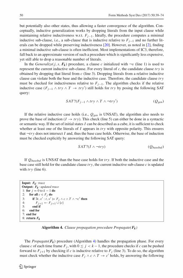
Input: Fk: traceOutput: Fk: updated trace1: for j = 0 to k − 1 do2: for all c ∈ Fj do3: if ∃t, v′ : t, v′ |� Fj ∧ c ∧ T ∧ ¬c′ then4: Fj+1 ← Fj+1 ∪ {c}5: end if6: end for7: end for8: return Fk

Algorithm 4. Clause propagation procedure Propagate(Fk)

The Propagate(Fk) procedure (Algorithm 4) handles the propagation phase. For everyclause c of each time frame Fj , with 0 ≤ j < k − 1, the procedure checks if c can be pushedforward to Fj+1 by checking if c is inductive relative to Fj (line 3). To do so, the algorithmmust check whether the inductive case Fj ∧ c ∧ T → c′ holds, by answering the following

123


SAT query:

SAT?(Fj ∧ c ∧ T ∧ ¬c′) (Qpush)

If the relative inductive case holds (i.e., Qpush is UNSAT), then c is relative inductive toFj and can thus be pushed forward to Fi+1. Otherwise, c can’t be pushed forward and theprocedure moves to the next iteration.

3 SAT solving requirements of IC3

In this section we analyse the SAT solving requirements of IC3 from the perspective ofits underlying SAT framework. From the standpoint of the SAT solving layer, the top-levelverification algorithm poses a sequence of SAT calls, each querying the satisfiability of adifferent CNF formula. A natural question arises regarding how different the CNF formulasof two subsequent SAT calls posed by IC3 are. Subsequent SAT calls may act on differenttime frames, thus involving different sets of frame clauses, may require the use of the propertyor the transition relation and may include some additional clauses and/or cubes. In general,thus, no strictly incremental or decremental pattern in the sequence of CNF formulas that IC3presents to the SAT framework can be identified. Some of the sub-formulas that compose IC3SAT queries are determined by the transition system and may appear unaltered in differentSAT calls. It is the case, for instance, of the property and transition relation clauses. Someother sub-formulas, such as time frames clauses, may appear in different SAT queries butthey grow incrementally as verification proceeds. Finally, some other sub-formulas are onlyrequired to answer a specific query. Examples of these query-specific clauses and cubes arethose appearing in relative induction checks.

A naïve approach to handle this sequence of SAT calls would be to use a new SAT solverinstance to handle each query, initializing it from scratch with the CNF formula of that query.Unfortunately, initializing a newSAT solver instance from scratch implies a certain overhead.Given the huge amount of SAT queries posed by a typical run of IC3, this approach would beprohibitively expensive for the algorithm. For this reason, state-of-the-art implementationsof IC3 resort to the use of SAT solvers exposing an incremental interface. Incremental SATinterfaces allow a sequence of SAT calls to be performed on a single solver, accommodatingthe loaded CNF formula between calls. This approach, besides reducing the overhead, alsoallows the SAT framework to reuse previously learned clauses when solving SAT queries.

Analysing the sequence of SAT calls posed by IC3, we can identify a set of features foran incremental SAT interface that are desirable for IC3. In particular, an incremental SATinterface for IC3 should support:

– Adding clauses to the CNF formula currently loaded in the solver;– Removing clauses from the CNF formula currently loaded in the solver;– Specifying variable assumptions to be used when solving the next SAT query.

Adding and removing clauses from the formula allow the SAT framework to use a singleincremental SAT solver instance to manage the whole sequence of SAT calls. In particular,the ability to remove clauses from the current CNF formula (alongside inferences derivingfrom such clauses) is required to handle query-specific clauses introduced by previous SATcalls (such as the candidate inductive clause in relative induction checks). Similarly, variableassumptions are needed as away to efficiently add query-specific cubes to the current formula.

123


Each literal of these cubes is treated as a variable assumption, enforced while solving theupcoming query and then forgotten by the solver.

Many SAT solvers, like MiniSAT [21], feature an incremental interface capable of addingnew clauses to the formula and to support variable assumptions. Removing clauses from theformula, however, is a complicated task andmany state-of-the-art SAT solvers do not directlysupport such a feature. This is because, when a clause C is being removed from the currentCNF formula, the solver must also track down and remove every learned clause deriving fromC . Although some solvers, such as zchaff [22], directly support clause removal, incrementalinterfaces such as the one exposed by MiniSAT are by far more common. In this work weassume the use of a SAT solver exposing a MiniSAT-like incremental interface.

Clause removal can be simulated through the use of variable assumptions and the intro-duction of additional variables, called activation variables, as described in [23]. The idea isthat clauses that may have to be removed from the solver are loaded augmented with a literal,called activation literal. Such a literal is obtained as the negation of a new variable, calledactivation variable. Activation variables are additional variables, introduced in the solver forthe purpose of clause removal and that should appear only in activation literals. Given a CNFformula F loaded into a SAT solver and a ∈ B an activation variable, we denote by Fa theset of clauses loaded with activation literal ¬a into the solver, i.e., the clauses of F in theform (C ∨ ¬a), where C is an original problem clause. The following lemma holds:

Lemma 5 Clauses in Fa do not influence the satisfiability of the formula F unless theiractivation variable a is asserted, i.e., assumed positive in the solver.

Considering the case in which a is not asserted, if a satisfying assignment τ for F \ Fa

exists, then the assignment τ ∧ a satisfies F . Vice-versa, if no satisfying assignment existsfor F \ Fa , then the same is true for F . Otherwise, if the activation variable a is asserted,activation literals in the clauses of Fa become falsified. Each clause of Fa , in the form(C∨¬a), thus reduces to the original clauseC and contributes with the rest of F to determinethe satisfiability of the loaded CNF formula.

Definition 19 Given a SAT solver S, a clause C and an activation variable a, we say that Cis a-activable in S iff the clause (C ∨ ¬a) is loaded into S. A clause C that is a-activable ina SAT solver S is said to be activated in S iff the literal a is assumed in S. A clause C thatis a-activable in a SAT solver S is said to be deactivated in S iff the unitary clause (¬a) isadded to S. Otherwise, C is said to be inactive.

Activated clauses become relevant for determining the satisfiability of the formula loadedin S. Deactivated clauses, instead, become satisfied (and are therefore made logically redun-dant) by the addition of a unitary clause asserting their activation literal. Note that everylearned clause derived by resolution from a deactivated clause will share its activation literaland therefore be deactivated as well. Whenever a SAT query has to be solved by a SATsolver S, if the query includes an a-activable clause C in S, then C has to be activated byadding a to its set of variable assumptions. Clause C remains activated as long as the queryis being solved, then it returns to the inactive state. Whenever a clause that is a-activable inS is not needed in the formula anymore, it must be deactivated. Deactivated clauses persistin the clause database of the solver until its periodical clause database cleaning procedureis executed. Inactive clauses are also redundant w.r.t. the loaded formula but they will notbe deleted by the solver during its periodical clause cleaning. Once a clause is deactivated itcannot be made inactive again.

The described approach to clause removal has the disadvantage of introducing one freshvariable in the solver per clause (or group of clauses) that must be removed. After a clause

123


is deactivated, depending on the solver implementation, its activation variable may stilloccupy some space in the internal data structures of the solver. Over time, the presenceof such variables can significantly degrade the SAT solver performance. Inactive clauses,albeit redundant w.r.t. the loaded formula, slow down the solver by occupying space in theclause database and in other data structures (the watch lists in particular). Also deactivatedclauses will continue to linger in the solver for some time, contributing to the solver slowdown meanwhile.

Given the highly local nature of its verification process, IC3 has proved to be highlysensitive both to the internal behaviours of SAT solvers and to the way its SAT solvingrequirements are handled at the implementation level. Different SAT solver setups and/orconfigurations may, in fact, lead to widely varying results in terms of performance. Alteringthe SAT solver configuration in any IC3 implementation may lead, for instance, to finddifferent CTIs during the cube blocking phase of the algorithm. These, in turn, may lead towhole different chains of proof obligations to be discharged. As a consequence, differentinductive lemmas can be derived and the algorithm may either converge faster or find itselfdwelling excessively on somepart of the state space, depending on the nature of those lemmas.

The scenario pictured above poses serious challenges for any implementation of the algo-rithm. Given a SAT solver exposing the required incremental interface, any implementationof IC3 must face the problem of deciding how to integrate the top-level algorithm with theunderlying SAT solving layer. In order to do so, three aspects must be considered:

– SAT solver allocation: decide howmany SAT solver instances to use and how to distributeSAT calls among them;

– SAT solver loading: decidewhich formula to incrementally load in each solver to correctlyanswer its SAT queries;

– SAT solver clean-up: decide when and how often each solver should be cleaned up toavoid performance degradation.

4 SAT queries in IC3

In order to gain some insight into how best to handle the SAT solving requirements of IC3, weanalysed the sequence of SAT queries it poses. Depending on the variant of IC3 considered,different sets of SAT queries may need to be answered.We base our analysis on the version ofthe algorithm presented in Sect. 2.5, which is also the one implemented in ourmodel checkingtool PdTRAV. Note that, although some of these queries can be considered structural to everyvariant of the algorithm, different variants of IC3 may involve different subsets of queries.

Three kinds of SAT queries can be identified:

– Queries that test the intersection between a set of states and a time frame;– Queries that check the inductive case for relative induction of a clause w.r.t. a time frame;– Queries that check the base case for relative induction of a clause w.r.t. a time frame.

We characterize each query both in terms of its kind and the role it plays in the verificationprocess. For instance, queries that check the relative inductive case for a clause play differentroles in the algorithm as they are used in several of its steps for different purposes: to find,generalize or push inductive lemmas. Following the description of the algorithm presentedin Sect. 2.5, we identify the queries reported in Table 1.

As previously stated, the base case for relative induction can be checked in either asyntactical or semantic way. Since the syntactic check is cheaper to perform, it is prioritizedin our implementation of the algorithm. In the problemswe consider the set of initial states can

123


Table 1 SAT queries breakdownin IC3 Name Role SAT query

Qtarget Target intersection SAT?(Fk ∧ ¬P)

Qblocked Blocked cube SAT?(Fi ∧ s)

Qrelind Relative induction SAT?(Fi ∧ ¬s ∧ T ∧ s′)Qgen Inductive generalization SAT?(Fi ∧ tr y ∧ T ∧ ¬tr y′)QbaseInd Base of induction SAT?(I ∧ ¬c)

QindPush Inductive push SAT?(Fj ∧ c ∧ T ∧ ¬c′)Qpush Clause propagation SAT?(Fi ∧ c ∧ T ∧ ¬c′)

always be represented as a cube. Therefore, the query QbaseInd will be excluded from the restof the analysis. From preliminary experiments, the inductive push optimization appears to bedetrimental to algorithm performance in the general case. Therefore we consider inductivepush disabled and exclude QindPush from the analysis. We also assume that the Extendprocedure described in Sect. 2.5 reduces proof obligation cubes using ternary simulation.

The following characteristics can be recognized for the different types of SAT queriesposed by IC3:

– Small-sized formulas each query includes at most a single instance of the transitionrelation;

– Large number of calls as the verification process of IC3 is highly localized, a large numberof reachability checks are required;

– Separate time frame contexts each SAT query focuses on a single time frame;– Related sequence of calls subsequent SAT calls arising from a given step of the algorithm

may expose a certain correlation.

On the one hand, given their small size, SAT queries posed by IC3 can be consideredtrivial to solve w.r.t. the ones posed by other SAT-based invariant verification algorithms. Onthe other hand, such a triviality is largely compensated by their number. This suggests thatIC3 implementations should prefer faster SAT solvers to more powerful ones. SAT queriesposed by IC3 operate on separate time frame contexts. This suggests that the most naturalstrategy for SAT solvers allocation would be to instantiate one SAT solver instance for eachtime frame and then use that instance to handle every SAT query regarding the particular timeframe. As mentioned is Sect. 3, in the general case, no strictly incremental or decrementalpattern in the sequence of SAT formulas posed by IC3 can be identified. However, restrictingthe focus only to some steps of the algorithm, some patterns can be observed. For instance,SAT calls performed during inductive generalization act on very similar formulas, where eachcall differs from the previous one only by one literal in a clause and one variable assumption.

We conducted an experimental characterization of IC3 SAT queries, running our imple-mentation of IC3 in its default configuration on the complete set of solved single propertybenchmarks of HWMCC 2014 and HWMCC 2015. The benchmark set is composed of 525different instances overall, of which 337 are UNSAT and 188 are SAT. In line with the com-petition settings, time and memory limits of 900s and 8GB respectively were enforced. InTable 2 we report the statistics collected. Data are presented differentiating between SATand UNSAT calls. For each type of SAT query we consider an average IC3 run and providethe number of calls performed and the total solving time. The first three columns report the

123


Table 2 Total number of calls and solving times of SAT queries in an average IC3 run

Query Avg. total number of calls Avg. total solving time (ms)

SAT UNSAT TOT % SAT UNSAT TOT %

Qtarget 324 20 344 0.61 1495 11 1506 0.41

Qblocked 2978 24 3002 5.31 2204 2 2206 0.59

Qrelind 1046 1933 2979 5.26 21,747 2532 24,279 6.55

Qgen 17,884 8473 26,357 46.57 70,104 5677 75,781 20.44

Qpush 15,781 8133 23,914 42.25 14,361 7889 22,250 6.00

Total 38,013 18,583 56,596 100 10,9912 16,110 126,021 33.99

average number of calls per query type and their percentage over the total number of calls.The last four columns report the total time spent, in an average run of IC3, solving queriesof each type as well as the percentage of execution time dedicated to each of them. Averagesare computed over the 525 instances of the benchmark set. Percentages of execution time arecomputed over the average execution time of the runs, equal to 370.75 s.

Concerning the volume of SAT calls for each query, we can derive the following consid-erations. A typical run of IC3 executes tens of thousands of SAT calls. SAT calls involvedin inductive generalization and clause propagation are by far the most frequent ones, rep-resenting almost 90% of the queries posed by an average execution of the algorithm. Thisis because, Qgen is called multiple times for each inductive clause found, potentially onetime for each of its literals. Also the query Qpush can be performed multiple times for everyinductive clause, potentially once or more for every propagation phase. As it may be expectedconsidering the procedure described in Sect. 2.5, the numbers of Qblocked and Qrelind callsare very close. Their disparity is mainly due to the benchmarks in which a counterexampleto the property is found. The number of target intersection calls is very small if compared tothe one of other queries. This suggests that IC3 does not need to explicitly enumerate a verylarge number of bad cubes before a time frame is proved safe.

Considering the proportion of SATs and UNSATs for each query, we can notice that forQblocked the number of UNSATs is extremely low. This suggests that proof obligation rarelybecomes discharged as a result of discharging a previously extracted one. Regarding Qrelind ,the higher number of UNSATs compared to SATs suggests that, when discharging a proofobligation, bad cubes are often found already relative inductive w.r.t. the previous time frame,i.e., the case in which a CTI is found is less frequent. In addition, it is interesting to noticethat both number and proportion between SATs and UNSATs for Qgen and Qpush are roughlythe same, suggesting that those queries are very similar in nature. For both query types, aSAT result is far more frequent than an UNSAT one. This means that many of the relativeinductive case checks performed during inductive generalization and clause propagation fail.

Analysing total solving times in Table 2, we can notice that, in an average run of IC3,about one third (34%) of the execution time is spent answering SAT queries. Most of thistime is spent answering inductive generalization queries, in particular the ones producing aSAT result. This suggests that, speeding up the solving time for this type of queries wouldgreatly improve overall algorithm performance. Despite presenting similar volumes of calls,queries Qgen and Qpush consume significantly different percentages of the execution time.

123


Table 3 Average solving time, number of decisions and CNF size of a single call for each query type

Query Avg. solving time (ms) Avg. number of decisions Avg. CNF size

SAT UNSAT SAT UNSAT Clauses Literals Variables

Qtarget 4.61 0.53 13,669 257 2205 5497 1187

Qblocked 0.74 0.07 1118 91 1047 2450 415

Qrelind 20.79 1.31 129,301 420 4396 11,736 2255

Qgen 3.92 0.67 3580 636 2573 7187 813

Qpush 0.91 0.97 1226 759 1074 2780 299

Average 6.19 0.71 29,779 432 2259 5930 994

In order to assess how difficult to solve the different queries are, in Table 3 we presentstatistics regarding the average solving time, number of decisions and size of single calls foreach query type. The size of each query is expressed in terms of the average number of clauses,variables and literals included in its CNF formula. Regarding average solving times of singlecalls, our measures suggest that solving satisfiable instances is by far more time consumingthan solving unsatisfiable ones. Solving time is tightly related to the number of decisionsrequired by each SAT query. Data reported in the third and fourth column of Table 3 showthat only a few decisions are needed to detect unsatisfiability, whereas recognizing satisfiableinstances requires a considerably higher number of decisions. Among the different types ofqueries, Qrelind appears to be the most difficult one to solve, both in terms of time and numberof decisions. This can be due in part to its size and in part to the fact that, differently fromQgen and Qpush, such a query often checks the relative induction of a certain clause w.r.t.a time frame for the first time. It is thus less likely for this type of queries to benefit fromprevious learning available in the solver.

In conclusion, Qrelind queries are the most difficult ones to solve but, given their limitednumber of calls, they do not burden the solver too much. Queries Qgen and Qpush are themost frequent ones, but Qgen seems to be significantly more difficult to solve than Qpush,resulting in a much more substantial load for the solver.

5 SAT solver allocation

The problem of SAT solver allocation in IC3 consists in deciding how many SAT solverinstances to employ and how to distribute the SAT solving work required by the algorithmamong them.Asmentioned in Sect. 3, the naïve approach comprising a throwawaySAT solverinstance for each query is not feasible. In order to limit the overhead due to SAT solver loadingand to exploit clause learning, we consider an incremental SAT solver exposing a MiniSAT-like interface. As noted in Sect. 4, many of the queries posed by IC3 share sub-formulas,primarily time frame clauses. On the one hand, solving queries that share a sub-formula usingthe same incremental SAT solver instance allows us to exploit clause learning and thus toavoid fruitless repetition of work. On the other hand, given the limitations of the incrementalSAT interface considered regarding clause removal, solving unrelated SAT queries with thesame solver instance can significantly degrade its performance over time.We aim at finding an

123


allocation of SAT queries to incremental SAT solver instances that achieves a good trade-offbetween these two opposing trends, allowing learning of useful clauses to be shared amongdifferent SAT calls but at the same time limiting performance degradation due to the presenceof redundant clauses and unused variables in the solver.

We distinguish two main approaches to SAT solver allocation:

– Monolithic solver a single solver is used to answer all queries;– One solver per time frame each time frame has its own dedicated solver.

In the monolithic solver approach, the set of clauses of each time frame must be loadedinto a single solver. Since SAT queries posed by IC3 act on separate time frame contexts,each time frame is assigned a different activation variable and its clauses are loaded inactiveinto the solver. To answer each SAT query, the appropriate time frame has to be activatedthrough literal assumptions. Similarly, the property is loaded inactive into the solver with itsown activation variable. If one solver per time frame is used, each solver is loaded only withthe set of clauses of its corresponding time frame and the inactive property clauses.

Both approaches have their advantages and shortcomings. On the one hand, using a mono-lithic solver allows learned clauses to be shared among every SAT query but the presence ofa large number of inactive clauses in the formula may degrade performance. On the otherhand, using one solver per time frame leads to symmetrical considerations. Deciding whichapproach is the best one is not trivial, as their performance results from a trade-off betweenthe aforementioned opposing trends and depends on the particular instance under verification.

Among state-of-the-art model checking tools, ABC and PdTRAV adopt the one solverper time frame approach, whereas nuXmv supports both approaches as well as an hybridapproach in which the first n time frames have their dedicated SAT solver and the remainingones share a single solver.

We propose the use of dedicated solvers to handle specific queries. For every solver,a secondary solver can be instantiated to handle all the queries of a specific type. Usingdedicated solvers to answer queries of a given type, will guarantee that any unnecessaryclause arising from them will not impact the performance of future queries of different types.Therefore, the main purpose of using dedicated solvers is not to directly affect solving timeof the queries being specialized, but rather to improve solving time of the other queries bypreventing many irrelevant clauses to accumulate in the solver, hindering its performance.

As noted in Sect. 4, inductive generalization and clause propagation are by far the mostfrequent SAT queries in IC3. Both types of query introduce a query-specific clause in thesolver, as well as some logic cones if lazy loading of the transition relation is used (seeSect. 6). Furthermore, some patterns can be recognized in the sequence of SAT calls per-formed during inductive generalization and clause propagation. SAT calls performed duringan execution of inductive generalization act on very similar formulas, where each call differsfrom the previous one only by a literal in a clause and a variable assumption. Regarding clausepropagation, we can identify correlations among the SAT checks performed in subsequentpropagation phases. When a clause fails to be propagated, the same clause will be checkedfor propagation w.r.t. the same time frame in the next propagation phase. These SAT callsonly differ by the inductive lemmas that were added to the given time frame between the twopropagation phases.

We suppose it would be beneficial for the algorithm to solve those queries using dedicatedsolvers. This way, the large number of deactivated clauses and unused variables arising fromthese queries would not impact on solving other queries. Note that, althought Qrelind querieshave a higher average solving time than Qpush ones, the formers are much less frequent thanthe latters and therefore the are not solved by dedicated solvers as they represent a lesser

123


source of irrelevant clauses. Furthermore, these related SAT queries would be solved by asolver whose internal state is not altered by the answering of other (unrelated) SAT calls inbetween. We call solvers dedicated to the handling of a particular type of query specializedsolvers. For each SAT solver used, a specialized solver is instantiated and maintained by theSAT solving framework. Depending of the SAT solver allocation strategy used, either a singlespecialized solver or one specialized solver per time frame are instantiated. We propose threedifferent specialized SAT solvers strategies:

– Specialized generalization each query of type Qgen is performedon the specialized solver;– Specialized push each query of type Qpush is performed on the specialized solver;– Specialized generalization+push both queries of type Qgen and Qpush are performed on

the specialized solver.

6 SAT solver loading

Prior to solving a SAT query, all the relevant clauses of its formula that are not alreadyloaded in the solver must be added to it. In order to minimize the number of loaded clausesto deactivate, we analyse the queries to identify what is the minimal subset of clauses thatare needed to answer each one. Many of the SAT queries posed by IC3 involve the use of thetransition relation. As mentioned in Sect. 2, the transition relation of the system is composedof many next-state function δi , one for each state variable xi , so that:

x ′i ≡ δi (X) ∀xi ∈ X

Each next-state function δi determines the next-state value of a state variable xi . Weassume these functions are represented as AIGs and that they can be transformed into CNFformulas by applying a CNF encoding technique. We refer to the CNF formula derived fromthe next-state function δi of a state variable xi as the logic cone of xi . Next-state functions ofdifferent state variables may share sub-formulas, i.e., their AIGs may share some gates and,as a consequence, their logic cones may share some clauses.

Analysing the SAT queries posed by IC3, we observe that, when a SAT query involvingthe use of the transition relation is posed, the next state variables of the system are alwaysconstrained by some cube c′. Such queries ask if there exists a state s of the system thatsatisfies some present-state constraints (such as the intersection of a time frame and a clause)and which can reach one of the states c′ in one transition. Being s a state that satisfies oneof these queries, since c′ is a cube, s must have a successor p′ such that p′ ∈ c′. Onlythe present state variables that appear in the logic cones of variables in c′ are relevant indetermining if such a state s exists. Therefore, only the logic cones of the variables in c′are needed to determine the satisfiability of the query. In order to minimize the size of theformula to be loaded into each solver, a common approach is to load, for every SAT callthat involves the transition relation, only the necessary logic cones. This loading strategy,called as lazy loading of transition relation, is used in various implementations of IC3, asthe ones of PdTRAV and ABC. Since different logic cones may share part of their clauses,the algorithm implementation must keep track of the portions of logic cones loaded in eachsolver. When a new logic cone must be loaded into a solver, only the clauses that it does notshare with any of the logic cones already loaded in the solver should be added.

In the general case, each query involving the transition relation may require different logiccones to be loaded into the solver. As verification proceeds, portion of unused logic conesaccumulate in the solver, degrading its performance as inactive clauses, deactivated clauses

123


and unused activation variables do. The size of logic cones to load depends on the particularCNF encoding technique employed to translate next-state functions of the transition relationinto CNF formulas. As mentioned in Sect. 2, different CNF encoding techniques may, infact, detect different functional blocks in the AIGs representing those functions as well astranslating a given functional block into different sets of clauses. Besides influencing thesize of the logic cones, choosing a CNF encoding technique also impacts on the propagationbehaviour inside the SAT solver [24].

We noticed that, disregarding the particular CNF encoding technique employed, the num-ber of logic cones clauses that need to be loaded into the solver can further be reduced byusing a particular CNF encoding scheme due to Plaisted and Greenbaum [25], henceforthcalled PG encoding. Given a next state cube c′ and the AIG representation C of the next-statefunctions of its variables, c′ can be seen as a set of constraints on the outputs of C. Therefore,the pair (C, c′) can be seen as a constrained Boolean circuit. PG encoding is a CNF encodingscheme that may be applied when translating a constrained Boolean circuit into a CNF for-mula with a given CNF encoding technique. The CNF formula obtained when applying PGencoding is a subset of the one obtained when applying the original CNF encoding techniqueby itself. Given a constrained circuit (C, c′) and a CNF encoding technique, translating Cinto a CNF formula F , PG encoding works by exploiting constraints on the outputs andtopological information on the circuit to remove some of the clauses of F , producing a CNFformula PG(F) that is equi-satisfiable to F . For some of the functional blocks detected bythe given CNF encoding technique, in fact, it is proved that an equi-satisfiable encoding canbe produced by only translating one of the two sides of their defining bi-implication (see[25] or [17]). PG encoding effectively reduces the size of CNF formulas, but it is not clearwhether or not it leads to worse propagation behaviour [26].

7 SAT solver clean-up

Inevitably, as verification proceeds, some redundant clauses and unused variables accumu-late in each solver degrading its performance. A solution to this problem is to periodicallydestroy each solver and to replace it with a fresh SAT solver instance. We refer to such anoperation as a SAT solver clean-up. Besides recollecting wasted memory in the SAT solverdata structures, this procedure has the added benefit to reset the internal state of the solverwhich over time might accumulate too much bias towards certain (possibly poor) choices.As a consequence, different bad cubes can be derived and blocked by IC3, leading the timeframes to be differently refined and, in turn, steering the overall verification process towarda different direction.

To clean up a SAT solver instance, a new instance is allocated and loaded with onlythose clauses that are actually pertinent to answer the upcoming SAT query. Local data ofthe solver, such as learned clauses, saved variable phases and score values of variables andclauses, are lost in the process. Therefore, cleaning up a SAT solver instance introduces acertain overhead, mainly because clauses pertinent to answer the upcoming SAT query mustbe loaded again in the solver and any useful inference previously derived by the solver mustbe derived again while solving the upcoming SAT call.

Deciding how frequently SAT solver instances must be cleaned up is an important aspectof IC3 implementation and can greatly influence the performance of the algorithm. Any IC3implementation must adopt a clean-up strategy, based on some heuristic measure, in order toachieve a trade-off between avoidance of performance degradation and clean-up overhead.The purpose of a clean-up strategy is to determine whether the number of irrelevant clauses

123


and/or variables (w.r.t. the upcoming query) currently loaded into a solver has become largeenough to justify a clean-up. To do so, we define a heuristic measure representing an estimateof the number of irrelevant clauses/variables currently loaded into a solver. Such a measureis then compared to some threshold and, if it exceeds it, the solver is cleaned up.

Clean-up strategies used in state-of-the-art model checking tools, such as ABC, PdTRAVand nuXmv, usually rely on loose estimates of the size of the irrelevant portion of the formulaloaded into each solver. Furthermore, these tools often use static thresholds to decide whetherthe computed estimates justify aSATsolver clean-up.BothPdTRAVandABCuse the numberof deactivated clauses as a measure of the number of irrelevant clauses in the solver (withouttaking into account unused logic cones), whereas nuXmv only considers the number ofincremental SAT calls.

We explore the use of novel clean-up heuristics, based on different measures of the numberof irrelevant clauses loaded into each solver and able to dynamically adjust the frequency ofclean-ups based on the locality of the verification process.

As stated before, upon receiving a new SAT call, two kinds of irrelevant clauses can bepresent into a SAT solver instance:

1. Deactivated and inactive clauses from previous inductive checks (such as Qrelind andQgen queries);

2. Portions of logic cones from previous SAT calls involving T that fall outside the logiccones of the upcoming query.

The actual number of irrelevant clauses in the solver depends both on the formula F cur-rently loaded into the solver and on the nature of the upcoming SAT query Q. We investigatethe use of a heuristic measure taking into account both sources of irrelevant clauses.

Given a SAT solver instance loaded with the formula F , and a SAT query Q(a) in whicha cube of activation literals a is assumed, the number of deactivated clauses d(F, a) in F issimply computed by adding a counter for each activation variable to the solver. Every timea clause with a given activation literal is added to the solver, the counter of the correspond-ing variable is incremented. The number of clauses of F currently deactivated for Q(a) iscomputed as the sum of the counters for each activation variable not in a.

Given a SAT solver instance loaded with the formula F and a SAT query Q(c′) whosesolution requires the logic cones of a cube c′ to be loaded in the solver, the number of irrelevanttransition relation clauses of F w.r.t. Q(c′), depends on F and the logic cones of c′. Logiccones of different state variables may, in fact, share some of their clauses, correspondingto the common gates in the AIG representation of their next-state function. The number oflogic cones clauses of F that are irrelevant to answer Q, denoted by u(F, c′), is computedas follows:

u(F, c′) = |T (F)| − |S(F, c′)|where |T (F)| is the number of transition relation clauses already loaded into the solver and|S(F, c′)| is the number of clauses that the logic cones of c′ share with the logic cones previ-ously loaded in the solver. In order to compute such a measure, the algorithm implementationmust keep track of the logic cones currently loaded in each solver and must be able to com-pute the number of shared clauses among different logic cones through an appropriate datastructure.

Given F and Q(c′), dividing u(F, c′) by the number of transition relation clauses in Fwe obtain the ratio of transition relation clauses in F that are irrelevant to solve the currentquery, denoted by U (F, c′):

123


U (F, c′) = u(F, c′)|T (F)|

We consider such a measure averaged on a sliding window W (U, n) of the last n SATcalls, in order to to dynamically adjust the frequency of clean-ups based on the locality of theverification process. As soon as the ratio of irrelevant transition relation clauses loaded in thesolver, averaged on the last n SAT calls, exceeds some predetermined threshold we assumethat the locality of the verification process has varied enough to deem the loaded logic conesfutile.

Given a solver instance loaded with F and a SAT query Q(c′), let |vars| be the totalnumber of variables in F , |act | be the number of activation variables in F , U (F, c′) be theratio of transition relation clauses in F that are irrelevant for c′ and W (X, n) be a slidingwindow containing the measures of X collected for the last n SAT calls of a solver. Weconsider the following four clean-up strategies:

|act| > 300 (H1)

|act| >1

2|vars| (H2)

avg(W

(U (F, c′), 1000

))> 0.5 (H3)

H2 || H3 (H4)

Clean-up strategy H1 is the default strategy implemented in PdTRAV and ABC. Eachsolver is cleaned up after a fixed number of variables are reserved for activation. Strategy H2,first proposed in [4], triggers SAT solvers clean-ups after half their variables are reservedfor activation. H3 is based on the heuristic measure proposed before and cleans up eachsolver after the average number of irrelevant transition relation clauses, computed over thelast thousand of calls, exceeds 50% of the total number of transition relation clauses. Finally,strategy H4combines the preceding two inorder to take into account both sources of irrelevantclauses.

8 Experimental results

We conducted an experimental evaluation of different SAT solver allocation, loading andclean-up strategies in IC3, considering the same set up described in Sect. 4.

Two sets of experiments were conducted on the IC3 implementation of three state-of-the-art model checking tools: PdTRAV, nuXmv and ABC. Section 8.1 shows results attainedwith PdTRAV on the full set of single property benchmarks of HWMCC 2014 and 2015. Asit turns out that most of the benchmarks can be considered easy model checking problems,Sect. 8.2 focuses on a core subset of experiments, onwhichwe present data for all threemodelcheckers. All experiments were performed by comparison with a baseline configurationof the tool. For PdTRAV and ABC, the default configuration was used as baseline; fornuXmv, the same baseline configuration considered in [16]was used.Asmostmodel checkersoperate some preprocessing (e.g., circuit reduction, signal and latch correspondence, phaseabstraction) before activating model checking engines, we performed off-line preprocessingwith PdTRAV, stored netlists on file, for fair comparison among the three model checkers.All of the three model checking tools considered make use of MiniSAT 2.2.0 as a back-endSAT solver. This helps us making more fair comparisons across the tools, excluding bias dueto the specific SAT solver implementation.

123


Table 4 Number of solved instances using specialized solvers w.r.t. baseline

Configuration Solved UNSAT SAT New UNSAT New SAT Lost UNSAT Lost SAT �baseline

Qgen spec. 311 225 86 4 1 4 3 −2

Qpush spec. 312 226 86 4 0 3 2 −1

Qgen + Qpush spec. 315 226 89 4 3 3 2 +2

Baseline 313 225 88 – – – – –

Virtual best 323 232 91 7 3 – – +10

Experimental results are reported by comparing different groups of techniques againstthe respective baseline. For each group, results are provided by means of a table, a sur-vival plot and a Venn’s diagram. Tables report the total number of solved instances andthe number of instances that are gained and lost by each technique w.r.t. the baseline. Foreach group, the corresponding table also reports the results of a virtual best configuration,obtained combining the results of all the compared techniques. Survival plots compare thenumber of solved instances of each technique in a group over time. Venn’s diagrams showhow the compared techniques relate in terms of mutually solved instances. For each tech-nique, within each group, we also provide a scatter plot to assess its impact on performancew.r.t. the baseline, using different graphical artefacts to represent different benchmark fam-ilies.

8.1 Experiments with PdTRAV on full benchmark set

We have run a full set of experiments over the 525 HWMCC 2014 and 2015 circuits, with a900s time limit and a 8GB memory limit. Experiments were run on an Intel Core i7−3770,with 8CPUs running at 3.40GHz, 16GB of main memory DDR III 1333, and hosting aUbuntu 12.04 LTS Linux distribution.

8.1.1 Experiments with specialized SAT solvers

We report the number of solver instances (differentiating SAT and UNSAT results) alongsidegains and losses and overall delta for each configuration w.r.t. our baseline.

As described before, we decided to specialize solvers in the context of Qgen and Qpush, inthree different configurations: only the former, only the latter and both at the same time. Wefocused our experiments on these two queries as they were the most frequent kind, as shownin Table 3.

Table 4 illustrates the role of specialized solvers, i.e., additional solvers per frame dedi-cated to a specific query, during IC3 runs. Such a table compares the three aforementionedspecialization configurations against our baseline, which instead uses a single unspecialisedsolver for each time frame.All the variants are rather close in terms of overall solved instances,but each of them is characterized by the presence of some unique solves, thus providing aslight contribution to the portfolio.

Figure 1 illustrates data distribution of solved instances for all the instances w.r.t. to thebaseline. Each sub-figure is dedicated to a specific variant, and each scatter plot represents themain circuit families with a different graphical style. Points that lie beneath the diagonal rep-

123


Fig. 1 Detailed comparison of different SAT solver specialization strategies versus the baseline. The baselineis always on the x-axis. Points below the diagonal characterize runs with a better performance. Points onborders represent time-outs. Different graphical artefacts visualize different benchmark families

(a)

050

100

150

200

250

300

320

0 25 50 75 100 125 150 175 200

Sol

ved

inst

ance

s

CPU Time [s]

BaselineGen

PushGenPush

300 400 500 600 700 800 900

(b)

Fig. 2 Detailed comparison of different specialized SAT solvers strategies on the complete benchmark set.a is a Venn’s diagram illustrating mutual coverage of solved instances among the compared strategies, b is asurvival plot illustrating distribution of solved instances over CPU time for each compared strategy

resent instances for which the alternative method performs better, in term of mere executiontime, than our baseline one. It is possible to notice that most of the points are rather close tothe diagonal, with few obvious exceptions. Analysing the full logs produced by PdTRAV, wenoticed that execution times for solved instances are rather close, regardless of the techniqueused. The main differences come from verification runs that end in time-out/memory-out forsome of the considered variants or, on the other hand, from unique solves.

Figure 2a presents the same results of Table 4 in a graphical way. Such a figure adoptsVenn’s diagrams to better illustrate the overlap among different techniques and to instantlyvisualize the subset on unique instances that each variant is capable of proving. Overlappingregions describe instances that are solved in common by different techniques, whereas outerlobes underline unique solves for each strategy.

Figure 2b illustrates data distribution of the number of solved instances w.r.t. increas-ing execution time. All the variants are plotted on the same survival chart to facilitate datacomparison. Once again, as already noticed while analysing scatter plots, it is rather straight-forward to remark how close all the variants are to one another. All the distributions presentedfollow somehow the same pattern. We can identify a large subset of easy instances that allthe proposed variants are capable of solving in a short amount of time, before encounteringharder instances.

123


Fig. 3 Detailed comparison of different CNF encodings versus the baseline

8.1.2 Experiments with CNF encodings

A second set of experiments evaluates the use of different encodings. Results were partlycontroversial, at least if compared with [16].

The baseline version of PdTRAV uses technology mapping encoding as proposed in [19].A run in PdTRAV using PG, with 900s time-out, showed a reduction in the number of solvedinstances from 313 to 302 (2 of which, a SAT instance and an UNSAT instance, previouslyunsolved). Overall, a decrease of performance, despite a reduction of dynamically loadedtransition relation clauses in the order of 20% for most of the considered circuits.

A first conclusion could be that PG encoding was not able to improve performance,suggesting it can indeed suffer of worst propagation behaviour. Nonetheless, it is interestingto observe that, combining the results of our baseline implementation with those obtainedwith PG encoding, the overall number of solved problems grows, albeit slightly, as the latterwas able to solve two instances that the former could not.

An interesting resultwas obtained using theTseitin encoding and an improved versionwithclauses for simple gate blocks (T and T+ for shortening, respectively). The two encodingsproved better than our baseline one, both in terms of sheer number of solved instances andin terms of solving time.

Figure 3 illustrates data distribution of solved instances w.r.t. to the baseline. On the onehand we can see that PG encoding tends to result in worse execution time that the baseline,with most of the points lying above the diagonal. On the other hand, T+, manages to improvethe baseline results for several instances.

Figure 4a presents the same results of Table 5 in a graphical way.Figure 4b illustrates data distribution of the number of solved instance w.r.t. increasing

execution time. All the variants are plotted on the same survival chart to facilitate datacomparison. Once again, it is surprising to observe the faster rate of convergence for the T+encoding, whereas PG stays constantly beneath the other two methods. Both axes feature anon-linear scale in order to better visualize the almost vertical slope on the left-hand side ofthe plot as well as the portion where the techniques start to plateau on its right-hand side. Inthis plot (and in all the following ones of the same kind) it is possible to notice a significantincrease of solved instances in the middle of the curve. This is due to a number of oski*instances, deriving from the same design, which are all solved roughly in the same amountof time.

We can conclude that T and T+ encodings seem to play better with incremental load oftransition relation clauses, as, though using more clauses that the baseline, due to a finergranularity. A different conclusion is driven in [16], probably due to the fact that the baseline

123


(a)

050

100

150

200

250

300

325

0 25 50 75 100 125 150 175 200

Sol

ved

inst

ance

s

CPU Time [s]

BaselinePGT+

T

300 400 500 600 700 800 900

(b)

Fig. 4 Detailed comparison of different specialized SAT solvers strategies on the complete benchmark set.a is a Venn’s diagram illustrating mutual coverage of solved instances among the compared strategies, b is asurvival plot illustrating distribution of solved instances over CPU time for each compared strategy

Table 5 Number of solved instances using different CNF encodings w.r.t. baseline


PG encoding 302 219 83 1 1 7 6 −11

Tseitin encoding 314 226 88 4 2 3 2 +1

Tseitin+encoding 320 233 87 8 0 1 1 +7

Baseline 313 225 88 – – – – –

Virtual best 327 236 91 10 3 – – +14

IC3 implementation in nuXmv does not use dynamic loading of the transition relation, thusproviding an ideal ground for a minimal clause set encoding.

8.1.3 Experiments with SAT solver clean-up strategies

The same set of experiments has been run taking into account different clean-up heuristics.Heuristic H1 is the clean-up heuristic used in the baseline version of PdTRAV. The static

threshold of 300 activation literals was determined experimentally. Heuristic H2 cleans upeach solver as soon as half its variables are used for activation literals. It can be seen as afirst simple attempt to adopt a dynamic clean-up threshold. Heuristic H3 is the first heuristicproposed to take into account the second source of irrelevant clauses described in Sect. 7,i.e., irrelevant portions of previously loaded cones. In H3 a solver is cleaned up as soon as thepercentage of irrelevant transition relation clauses loaded, averaged on a window of the last1000 calls, reaches 50%. Heuristic H4 takes into account both sources of irrelevant clauses,combining H2 and H3.

Table 6 shows a comparison among H1 (our baseline), H2, H3, and H4 respectively.Among dynamic threshold heuristics, both H2 and H3 take into account a single source ofirrelevant loaded clauses, respectively the deactivated clauses in H2 and the unused portions

123


Table 6 Test or restart strategies w.r.t. baseline

Configuration Solved UNSAT SAT NewUNSAT

NewSAT

LostUNSAT

LostSAT

�baseline

Variable activation (H2) 314 227 87 4 3 2 4 +1

Windowed (H3) 304 221 83 2 0 6 5 −9

Double threshold (H4) 310 226 84 4 1 3 5 −3

Baseline (H1) 313 225 88 – – – – –

Virtual best 321 230 91 5 3 – – +8

Fig. 5 Detailed comparison of different SAT solver restart strategies versus the baseline

of transition relation in H3. Data clearly indicates that H3 has worse performance. Thissuggests that deactivated clauses play a bigger role in degrading SAT solvers performancethan irrelevant transition relation clauses do. Taking into account only the latter source ofirrelevant clauses is not sufficient.

Figure 5 illustrates data distribution of solved instances for all the instances w.r.t. to thebaseline. In this figure, note that the points are still fairly close the diagonal, like in Fig. 1,but in this case data variance is a bit larger as restart strategies may significantly impact onoverall solving time.

Figure 6a presents the same results of Table 6 in a graphical way.Figure 6b illustrates data distribution of the number of solved instance w.r.t. increasing

execution time. All the variants are plotted on the same survival chart to facilitate datacomparison. In the context of restart strategies, despite a similar progression among datadistributions, it is possible to notice a faster convergence of our baseline technique, whichlies above all the other lines for roughly the first third of execution times. After this, all thetechniques, with the exception of the windowed approach, fight for the lead, with the variableactivation one proving the best, in terms of overall number of solved instances, in the end.

8.2 Experiments on core benchmark set

We noticed that, among the solved instances, a significant number could be handled in lessthan 10% of the allotted time (i.e., 90 s) by the baseline and all the variants alike. Such subsetof benchmarks, that we consider a core set for experimental evaluation, is composed of 223instances, of which 188 are UNSAT and 35 are SAT. All experimental data in this subsection,

123


(a)

050

100

150

200

250

300

320

0 25 50 75 100 125 150 175 200

Sol

ved

inst

ance

s

CPU Time [s]

BaselineWindowVarActDouble

300 400 500 600 700 800 900

(b)

Fig. 6 Detailed comparison of different SAT solver cleanup strategies on the complete benchmark set. a is aVenn’s diagram illustrating mutual coverage of solved instances among the compared strategies, b is a survivalplot illustrating distribution of solved instances over CPU time for each compared strategy

Table 7 Comparison of all the tested techniques purged of easy instances w.r.t. to baseline


NewSAT

LostUNSAT

LostSAT

�baseline

Generalize spec. 88 37 51 4 1 4 3 −2

Push spec. 89 38 51 4 0 3 2 −1

Gen+Push spec. 92 38 54 4 3 3 2 +2

Variable activation 91 39 52 4 3 2 4 +1

Windowed 81 33 48 2 0 6 5 −9

Double threshold 87 38 49 4 1 3 5 −3

PG 79 31 48 1 1 7 6 −11

T+ 97 45 52 8 0 0 1 +7

T 91 38 53 4 2 3 2 +1

Baseline 90 37 53 – – – – –

Virtual best 108 50 58 13 5 – – +18

obtained with PdTRAV, nuXmv and ABC, refer to this set. We propose the same kind ofvisual representation and data analysis presented in the previous section. Overall, pruningaway easy problems gives a better evaluation of the improvements obtained.

8.2.1 Experiments with PdTRAV

Table 7 compares the results of all the techniques we experimented with, w.r.t. the baseline,underlying gains and losses for each one. We deem that excluding the bulk of easy instancesfrom the presented results allows for a better representation of the impact of the differenttechniques in terms of overall achievable coverage.

123


(a)

0

20

40

60

80

100

0 100 200 300 400 500 600 700 800 900

Solv

ed in

stan

ces

CPU Time [s]

BaselinePGT+T

(b)

Fig. 7 Detailed comparison of different CNF encodings strategies on non-trivial instances. a is a Venn’sdiagram illustrating mutual coverage of solved instances among the compared strategies, b is a survival plotillustrating distribution of solved instances over CPU time for each compared strategy

(a)

0

20

40

60

80

100

0 100 200 300 400 500 600 700 800 900

Sol

ved

inst

ance

s

CPU Time [s]

BaselineGen

PushGenPush

(b)

Fig. 8 Detailed comparison of different specialized SAT solvers strategies on non-trivial instances. a isa Venn’s diagram illustrating mutual coverage of solved instances among the compared strategies, b is asurvival plot illustrating distribution of solved instances over CPU time for each compared strategy

Figure 7a, b visually represent as a Venn’s diagram and as a survival plot, respectively,the data reported in Table 7 for CNF encodings strategies. In this case, the survival plot iscreated with linear axis given the slope of the plotted curves. This holds for the followingsurvival plots as well.

Figure 8a, b visually represent as a Venn’s diagram and as a survival plot, respectively,the data reported in Table 7 for specialized SAT solvers strategies.

Figure 9a, b visually represent as a Venn’s diagram and as a survival plot, respectively,the data reported in Table 7 for SAT solver clean-up strategies.

8.2.2 Experiments with different SAT solver tunings

As stated before, IC3 is highly sensitive to the way its SAT solving requirements are handled.Besides choosing among different SAT solvers management strategies, another determiningfactor for the algorithm’s performance is deciding how to tune the internal behaviour of the

123


(a)

0

20

40

60

80

100

0 100 200 300 400 500 600 700 800 900

Sol

ved

inst

ance

s

CPU Time [s]

BaselineWindowVarActDouble

(b)

Fig. 9 Detailed comparison of different SAT solver clean-up strategies on non-trivial instances. a is a Venn’sdiagram illustrating mutual coverage of solved instances among the compared strategies, b is a survival plotillustrating distribution of solved instances over CPU time for each compared strategy

SAT solver. In order to evaluate the impact of different SAT solver tunings, we experimentedwith different settings for the clause deletion strategy of MiniSAT. In particular, we areinterested in assessing whether or not varying the aggressiveness of the clause deletionstrategy, instead or in conjunctionwith SAT solver restart strategies, could lead to a differencein terms of performance and/or coverage.

We isolated two parameters regulating the aggressiveness of the clause deletion strategyof MiniSAT: the deletion trigger threshold and the deletion ratio. The former defines thepercentage of learnt clauses, w.r.t. to the original number of problem clauses, required totrigger a cleanup of the clause database. The latter defines the minimum percentage of learntclauses to forget at each cleanup. Clauses are removed according to an activation-basedheuristics. In MiniSAT the default values for these thresholds are 33 and 50% respectively.

We have run a first set of experiments using different values for those thresholds, ona subset of the harder instances. Our goal was to evaluate the impact or more aggressiveand less aggressive deletion strategies on the overall procedure. We selected 20, 33 and100% as cleanup thresholds and 25, 50 and 75% as deletion ratio, for a total of nine differentexperimental configuration. Experiments were run on PdTRAV’s baseline configuration afterchanging the settings of the underlying MiniSAT solver.

Preliminary results proved to be rather consistent with our baseline. Taking into accountsolved instances, the execution times improved of more than 10 for 4.91% of the test cases,whereas they worsened of more than 10 for 5.72% of the cases. Almost 15% of previouslysolved instances, though, resulted in execution timeout. Nevertheless, the most favourableresults derived from anticipated cleanups (using cleanup triggers of 20 or 33% instead of50%) but less aggressive deletion (just 50% instead of 75%). Overall, the best combinationproved to be 20% as cleanup trigger and 50% deletion ratio, which increased the coverageof our baseline configuration by 2. This seems to suggest that non useful clauses quicklyaccumulate in the solver’s database, but, at the same time, the activity-based heuristic ofMiniSAT is effective in recognizing and deleting them.

On these premises, we conducted a second set of experiments, testing our winning combi-nation of cleanup thresholds on thewhole set of hard instances.We tested thismore aggressiveclause deletion strategy, called early clause deletion (ECD), in conjunction with PdTRAV’sbaseline configuration as well as the most performing ones among our specialization andrestarting strategies. Results are summarized in Table 8.

123


Table 8 Comparison of different configurations using early clause deletion w.r.t. to baseline


NewSAT

LostUNSAT

LostSAT

�baseline

Baseline+ECD 77 29 48 3 0 11 5 −13

Gen+Push spec.+ECD 81 31 50 3 0 9 3 −9

Variable activation+ECD 77 29 48 3 0 11 5 −13

Baseline 90 37 53 – – – – –

Table 9 Comparison of a subset of SAT solvers management techniques run in nuXmv


Single+spec 102 48 54 1 1 0 0 +2

Multi+spec 96 43 53 3 2 7 2 −4

VarAct 95 42 53 3 3 8 3 −5

Multi 97 42 55 3 4 8 2 −3

Baseline 100 47 53 – – – – –

Virtual best 109 52 57 5 4 – – +9

Introducing early clause deletion it was possible to increase PdTRAV coverage by threemore circuits. However, at the same time, the specific variants seemed to perform worse,on average, at least in terms of sheer number of solved instances. Nevertheless, it seemsplausible that a more careful tuning of the solver parameters (e.g., devising clause deletionstrategies specifically tailored for IC3) may lead to performance improvements. We leavesuch an investigation as future work.

8.2.3 Experiments with NuXmv

We have conducted a subset of the aforementioned experimental analysis on another state-of-the-art model checking tool, nuXmv, in order to gather more data. Furthermore, nuXmvnatively supports both single solver and multiple solvers approaches, whereas the former isnot currently available in PdTRAV. This allowed us to inquire further in this direction as well.

We have run nuXmv in both its single and multiple solvers variants, as well as introducingsome tweaks to the code to test some of our proposed techniques. We extended its capabilityto support specialized solvers, in order to test the best configurationwe found: Qgen and Qpush

specialized.We also introduced a different way to handle SAT solvers restart, introducing ourvariable activation strategies. Implementing also the windowed approach just to be able totest our double threshold strategy, seemed somewhat unnecessarily expensive. Furthermore,as the windowed approach impacts on the way the transition relation is loaded, it could haveled us to significantly alter the nature of the tools. This is something we wanted to avoid.

We took into account only a subset of the benchmarks, running experiments only on thesubset of non-trivial aforementioned instances.

Table 9 represents a summary of nuXmv runs against its own possible configurationsand the virtual best results. It is possible to notice how the single solver implementation of

123


0

20

40

60

80

100

0 100 200 300 400 500 600 700 800 900

Sol

ved

inst

ance

sCPU Time [s]

BaselineMulti

Multi+SpecSingle+Spec

VarAct

(a) (b)

Fig. 10 Experimental analysis with nuXmv. a Detailed comparison of different SAT solver managementstrategies, represented as Venn’s diagram, b detailed comparison of different SAT solver management strate-gies, represented as survival plot

Table 10 Comparison of a subset of SAT solvers management techniques run in ABC


NewSAT

LostUNSAT

LostSAT

�baseline

Monolithic 95 42 53 5 0 7 4 −6

R1 101 46 55 6 0 4 2 +0

R2 96 42 54 2 1 4 4 −5

Baseline 101 44 57 – – – – –

Virtual best 110 52 58 8 1 – – +9

nuXmv is the most performing one, with a further increase in solved instances when weenable specialized solvers. The differences among all runs are minimal, at least in terms ofsheer number of solved instances, but is still possible to notice a significant increase in termof overall coverage.

To better characterize the peculiarity of each tool and configuration, we use once moreVenn’s diagrams. At the same time, we plot as a survival plot the number of solved instancesover increasing solving time, to provide a feedback concerning techniques convergence.

Figure 10a graphically illustrates the regions of overlap among techniques as well as themore interesting unique solves. Furthermore, it is possible to infer the grade of orthogonalityamong tools and configurations, stemming from the subsets of mutually unsolved instances.

Figure 10b graphically illustrates as a survival plot the number of solved instances overincreasing verification time.

8.2.4 Experiments with ABC

We have conducted a subset of the aforementioned experimental analysis on ABC, as well.Following the same strategies used for nuXmv, we have excluded from further experimenta-tion the subset of trivial instances, focusing on the more interesting ones.

123


0

20

40

60

80

100

0 100 200 300 400 500 600 700 800 900

Sol

ved

inst

ance

s

CPU Time [s]

MonolithicR1R2R2

(a) (b)

Fig. 11 Experimental analysis with ABC. aDetailed comparison of different SAT solver management strate-gies, represented as Venn’s diagram, b detailed comparison of different SAT solver management strategies,represented as survival plot

Given the nature and structure of ABC, it was possible to run just a subset of the intendedexperiments, mainly focusing on restart strategies and transition relation loading.

Table 10 reports in row Baseline the default setting of ABC. Row Mono shows a runwithout dynamic transition relation clause loading (i.e., ABC with a monolithic approach).Row R1 shows a different period for solver clean-up (1000 variables instead of 300) whereasrow R2 shows a different restart strategy, mirroring the aforementioned variable activationapproach.

Figure 11a graphically illustrates the regions of overlap among techniques as well as themore interesting unique solves. Furthermore, it is possible to infer the grade of orthogonalityamong tools and configurations, stemming from the subsets of mutually unsolved instances.

Figure 11b graphically illustrates as a survival plot the number of solved instances overincreasing verification time.

Overall, results are in line with previous tools, showing that an increase in the number ofsolved problems (from 101 to 110), which indicate a potential improvement for a portfolio-based tool, able to concurrently exploit multiple settings.

9 Conclusions

The paper presents a detailed characterization and analysis of SAT queries posed by IC3,taking into account a subset of the most recent HWMCC benchmarks available. We alsodiscuss new ideas for solver allocation, loading and/or restarting. Experimental evaluation,performed considering three different state-of-the-art academic tools, shows lights and shad-ows as no breakthrough or clear winner emerges from the new ideas. Still, it is possible toappreciate the contribution each technique could bring to a portfolio-based model checkingenvironment.

PG encoding have shown to be less effective than expected. This is probably because thebenefits introduced in terms of loaded formula size are overwhelmed by the supposed worstpropagation behaviour of that formula, whereas finer grained encodings surpassed initialexpectations.

123


The use of specialized solvers seems to be effective when a static clean-up heuristic isused.

Our experiments showed that, when a dynamic clean-up heuristic is used, IC3 performancecan be improved by taking into account both deactivated clauses and irrelevant portions ofpreviously loaded cones.

The results are more interesting if we consider them from the standpoint of a portfolio-based tool, since the overall coverage (by the union of all set ups) is definitely higher.Evermore so if we focus on harder instances, rather that let the bulk of trivial ones obfuscateinteresting cases with their number.

So we believe that, despite the need for more effort in implementation, experimentation,and detailed analysis of case studies, this work contributes to the discussion of new devel-opments in research related to IC3. The lack of a winner-take-all technique is in line withmany related works and engineering efforts in the area of SAT-based model checking, andspecifically IC3. As a matter of fact, any specific optimization can improve on a set (or fam-ily) of model checking problems, while losing ground on other ones (as clearly confirmed byour experiments). Overall, given the intrinsic difficulty of characterizing families of bench-marks and relating them to best working techniques and setups, the improved portfolio canbe considered as the real final outcome.

Whereas other papers explore the area of algorithmic improvements within IC3 algo-rithms, or within SAT solvers, we focused on managing IC3 SAT queries in order to improveperformance, given a state-of-the-art general purpose SAT solver.

As future works we plan to follow two directions: devise better SAT solving manage-ment strategies and shift the focus on internal details of SAT solvers. The former requiresto keep investigating in the same direction of this paper, in order to identify a subset ofwinning SAT solver management schemes while considering solvers as black boxes. A pos-sible development in this direction would be to consider a more flexible incremental SATinterface capable of deleting clauses without the need of activation variables. This can bedone by taking advantage of resolution-based solvers as shown in [27], in the context ofMUS extraction. The latter requires to investigate in more depth how to tune a SAT solveror how to tailor its internal procedures to best fit IC3 needs. A possible follow-up work inthis direction could be to take into account different SAT solver implementations or solversbased on different forms of presenting the satisfiability problem. In particular it would beinteresting to investigate the use of hybrid SAT solvers such as CirCUs [28] in this con-text.

References

1. Cabodi G, Mishchenko A, Palena M (2013) Trading-off incrementality and dynamic restart of multiplesolvers in IC3. DIFTS, Portland

2. Bradley AR (2011) SAT-based model checking without unrolling. VMCAI, Austin3. Biere A, Jussila T (2008) The model checking competition web page. http://fmv.jku.at/hwmcc. Accessed

Feb 20174. Eén N, Mishchenko A, Brayton RK (2011) Efficient implementation of property directed reachability.

FMCAD, Austin, pp. 125–134. ISBN:978-0-9835678-1-35. Biere A, Cimatti A, Clarke EM, FujitaM, ZhuY (1999) SymbolicModel Checking using SAT procedures

instead of BDDs. In: Proceedings of the 36th design automation conference on New Orleans, Louisiana.IEEE Computer Society, June 1999, pp 317–320. DOI:10.1145/309847.309942

6. SheeranM, Singh S, Stålmarck G (2000) Checking safety properties using induction and a SAT solver. In:Hunt WA, Johnson SD (eds) Proceedings of the formal methods in computer-aided design series, LNCS,vol 1954. Springer, Austin, November 2000, pp 108–125. ISBN:3-540-41219-0

123

http://fmv.jku.at/hwmcc

http://dx.doi.org/10.1145/309847.309942


7. Bjesse P, Claessen K (2000) SAT-based verification without state space traversal. In: Proceedings ofthe formal methods in computer-aided design, series, LNCS, vol 1954. Springer, Austin, pp 372–389.ISBN:3-540-41219-0

8. McMillan KL (2003) Interpolation and SAT-basedmodel checking. In: Proceedings of the computer aidedverification, series. LNCS, vol 2725. Springer, Boulder, pp 1–13. doi:10.1007/978-3-540-45069-6_1

9. Bradley AR (2012) Understanding IC3. In: Cimatti A, Sebastiani R (eds) SAT series Lecture Notes inComputer Science, vol 7317. Springer, pp. 1–14. doi:10.1007/978-3-642-31612-8_1

10. Cabodi G, Nocco S, Quer S (2011) Benchmarking a model checker for algorithmic improvements andtuning for performance. Form Methods Syst Des 39(2):205–227. doi:10.1007/s10703-011-0123-3

11. Mishchenko A (2007) ABC: a system for sequential synthesis and verification. http://www.eecs.berkeley.edu/~alanmi/abc/. Accessed Feb 2017

12. Cavada R, Cimatti A, Dorigatti M, Griggio A, Mariotti A, Micheli A, Mover S, Roveri M, Tonetta S(2014) The nuxmv symbolic model checker. In: Biere A, Bloem R (eds) Proceedings of the computeraided verification, series. LectureNotes inComputer Science, vol 8559. Springer International Publishing,pp 334–342. doi:10.1007/978-3-319-08867-9_22

13. Hassan Z, Bradley AR, Somenzi F (2013) Better generalization in IC3. FMCAD, Portland, pp 57–16414. Vizel Y, Grumberg O, Shoham S (2012) Lazy abstraction and SAT-based reachability in hardware model

checking. FMCAD, Cambridge, pp 173–18115. Chockler H, Ivrii A, Matsliah A, Moran S, Nevo Z (2011) Incremental formal verification of hardware.

FMCAD, Austin, pp 135–14316. Griggio A, Roveri M (2015) Comparing different variants of the IC3 algorithm for hardware model

checking. IEEE Trans Comput Aided Des. doi:10.1109/TCAD.2015.248186917. Järvisalo M, Biere A, Heule M (2012) Simulating circuit-level simplifications on CNF. J Autom Reason

49(4):583–619. doi:10.1007/s10817-011-9239-918. Tseitin GS (1983) On the complexity of derivation in propositional calculus. In: Automation of reasoning:

2: classical papers on computational logic 1967–1970. pp 466–483. doi:10.1007/978-3-642-81955-1_2819. Eén N, Mishchenko A, Sörensson N (2007) Applying logic synthesis for speeding up SAT. Theory and

applications of satisfiability testing, series, LNCS, vol 4501. Springer, Lisbon, May 28–31 2007, pp272–286. doi:10.1007/978-3-540-72788-0_26

20. Bradley AR, Manna Z (2007) Checking safety by inductive generalization of counterexamples to induc-tion. FMCAD, Austin, pp 173–180. doi:10.1109/FAMCAD.2007.15

21. Eén N, Sörensson N (2016) The minisat SAT solver. http://minisat.se. Accessed Feb 201722. Moskewicz M, Madigan C, Zhao Y, Zhang L, Malik S (2001) Chaff: engineering an efficient SAT solver.

In: Proceedings of the 38th design automationConference on LasVegas, Nevada. IEEEComputer Society,June 2001. doi:10.1145/378239.379017

23. Eén N, Sörensson N (2003) Temporal induction by incremental sat solving. Electron Notes Theor ComputSci 89(4):543–560. doi:10.1016/S1571-0661(05)82542-3

24. Björk M (2009) Successful SAT encoding techniques. In: Journal on satisability, boolean modeling andcomputation. Addendum, IOS Press

25. Plaisted DA, Greenbaum S (1986) A structure-preserving clause form translation. J Symb Comput2(3):293–304. doi:10.1016/S0747-7171(86)80028-1

26. Eén N (2007) Practical sat: a tutorial on applied satisfiability solving. Slides of invited talk at FMCAD,2007. www.cs.utexas.edu/users/hunt/FMCAD/2007/presentations/practicalsat.html. Accessed 02 May2016

27. Nadel A, Ryvchin V, Strichman O (2013) Efficient MUS extraction with resolution. FMCAD, Portland,pp 197–200

28. Jin H, Somenzi F (2005) CirCUs: a hybrid satisfiability solver. In: Theory and applications of satisfiabilitytesting. Vancouver, BC, Canada, 2005. pp 211–223. doi:10.1007/11527695_17

123

http://dx.doi.org/10.1007/978-3-540-45069-6_1

http://dx.doi.org/10.1007/978-3-642-31612-8_1

http://dx.doi.org/10.1007/s10703-011-0123-3

http://www.eecs.berkeley.edu/~alanmi/abc/

http://www.eecs.berkeley.edu/~alanmi/abc/

http://dx.doi.org/10.1007/978-3-319-08867-9_22

http://dx.doi.org/10.1109/TCAD.2015.2481869

http://dx.doi.org/10.1007/s10817-011-9239-9

http://dx.doi.org/10.1007/978-3-642-81955-1_28

http://dx.doi.org/10.1007/978-3-540-72788-0_26

http://dx.doi.org/10.1109/FAMCAD.2007.15

http://minisat.se

http://dx.doi.org/10.1145/378239.379017

http://dx.doi.org/10.1016/S1571-0661(05)82542-3

http://dx.doi.org/10.1016/S0747-7171(86)80028-1

www.cs.utexas.edu/users/hunt/FMCAD/2007/presentations/practicalsat.html

http://dx.doi.org/10.1007/11527695_17

Documents

SAT solver management strategies in IC3: an …alanmi/publications/2017/fmsd17... · Form Methods Syst Des (2017) 50:39–74 DOI 10.1007/s10703-017-0272-0 SAT solver management strategies