SAS/IML Software: Changes and Enhancements, … ® Software: Changes and Enhancements, Release 8.1 The correct bibliographic citation for this manual is as follows: SAS Institute Inc.,

SAS/IML® Software: Changes and Enhancements,Release 8.1

The correct bibliographic citation for this manual is as follows: SAS Institute Inc.,SAS/IML® Software: Changes and Enhancements, Release 8.1, Cary, NC: SAS InstituteInc., 2000

SAS/IML® Software: Changes and Enhancements, Release 8.1

Copyright 2000 by SAS Institute Inc., Cary, NC, USA.

ISBN 1-58025-707-0

All rights reserved. Produced in the United States of America. No part of this publicationmay be reproduced, stored in a retrieval system, or transmitted, in any form or by anymeans, electronic, mechanical, photocopying, or otherwise, without the prior writtenpermission of the publisher, SAS Institute Inc.

U.S. Government Restricted Rights Notice. Use, duplication, or disclosure of thissoftware and related documentation by the U.S. government is subject to the Agreementwith SAS Institute and the restrictions set forth in FAR 52.227-19 Commercial ComputerSoftware-Restricted Rights (June 1987).

SAS Institute Inc., SAS Campus Drive, Cary, North Carolina 27513.

1st printing, May 2000

SAS and all other SAS Institute Inc. product or service names are registered trademarksor trademarks of SAS Institute Inc. in the USA and other countries. indicates USAregistration.

IBM® and all other International Business Machines Corporation product or servicenames are registered trademarks or trademarks of International Business MachinesCorporation in the USA and other countries.

Oracle® and all other Oracle Corporation product or service names are registeredtrademarks or trademarks of Oracle Corporation in the USA and other countries.

Other brand and product names are registered trademarks or trademarks of theirrespective companies.

Table of Contents

Chapter 1. Changes and Enhancements . . . . . . . . . . . . . . . . . . . . . . . . . . 1

Subject Index . . . . . . . . . . . . . . . . . . . . . . . . . . . . . . . . . . . . . . . 37

Syntax Index . . . . . . . . . . . . . . . . . . . . . . . . . . . . . . . . . . . . . . . . 39

Chapter 1Changes and Enhancements

Chapter Table of Contents

OVERVIEW . . . . . . . . . . . . . . . . . . . . . . . . . . . . . . . . . . . 3

FINANCIAL FUNCTIONS . . . . . . . . . . . . . . . . . . . . . . . . . . . 3

ROBUST REGRESSION . . . . . . . . . . . . . . . . . . . . . . . . . . . . 10

MULTIVARIATE TIME SERIES ANALYSIS . . . . . . . . . . . . . . . . . 29

REFERENCES . . . . . . . . . . . . . . . . . . . . . . . . . . . . . . . . . . 36

2 � Chapter 1. Changes and Enhancements

Chapter 1Changes and Enhancements

Overview

New financial functions, robust regression subroutines, and subroutines related tomultivariate time series analysis have been added. All necessary details such as argu-ments and operands are included.

Financial Functions

The following functions that compute information about financial quantities havebeen added:

CONVEXIT Function

calculates and returns a scalar containing the convexity of a noncontingent cashflow

CONVEXIT(times,flows,ytm)

The CONVEXIT function calculates and returns a scalar containing the convexity ofa noncontingent cash flow.

times is ann-dimensional column vector of times. Elements should be non-negative.

flows is ann-dimensional column vector of cash flows.

ytm is the per-period yield-to-maturity of the cash-flow stream. This is ascalar and should be positive.

Convexity is essentially a measure of how duration, the sensitivity of price to yield,changes as interest rates change:

C =1

P

d2P

dy2

With cash flows that are not yield-sensitive, and the assumption of parallel shifts to aflat term-structure, convexity is given by

C =

PKk=1 tk(tk + 1) c(k)

(1+y)tk

P (1 + y)2


whereP is the present value,y is the effective per period yield-to-maturity,K is thenumber of cash flows, and thek-th cash flow isc(k) tk periods from the present.

The statements

timesn=T(do(1,100,1));flows=repeat(10,100);ytm=0.1;convexit=convexit(timesn,flows,ytm);print convexit;

result in the following output:

CONVEXIT199.26229

DURATION Function

calculates and returns a scalar containing the modified duration of a noncontin-gent cash flow

DURATION(times,flows,ytm)

The DURATION function returns the modified duration of a noncontingent cash flowas a scalar.



ytm is the per-period yield-to-maturity of the cash-flow stream. This is ascalar and should be positive.

Duration of a security is generally defined as

D = �dPP

dy

In other words, it is the relative change in price for a unit change in yield. Sinceprices move in the opposite direction to yields, the sign change preserves positivityfor convenience. With cash flows that are not yield-sensitive, and the assumption ofparallel shifts to a flat term-structure, duration is given by

Dmod =

PKk=1 tk

c(k)(1+y)tk

P (1 + y)

whereP is the present value,y is the per period effective yield-to-maturity,K is thenumber of cash flows, and thek-th cash flow isc(k), tk periods from the present. This

FORWARD Function � 5

measure is referred to asmodified durationto differentiate it from the first durationmeasure ever proposed,Macaulay duration:

DMac =

PKk=1 tk

c(k)(1+y)tk

P

This expression also reveals the reason for the name duration, since it is a present-value-weighted average of the duration (that is, timing) of all the cash flows and ishence an “average time-to-maturity” of the bond.

For example, the statements below

times={1};ytm={0.1};flow={10};duration=duration(times,flow,ytm);print duration;

produce the output

DURATION0.9090909

FORWARD Function

calculates a column vector of forward rates given vectors of spot rates and times

FORWARD(times,spot–rates)

The FORWARD function returns ann� 1 vector of forward rates.

times is ann�1 column vector of times in consistent units. Elements shouldbe non-negative.

spot–rates is ann� 1 column vector of corresponding per-period spot rates. Ele-ments should be positive.

The FORWARD function transforms the given spot rates as

f1 = s1

fi =

�(1 + si)

ti

(1 + si�1)ti�1

� 1

ti�ti�1

� 1; i = 2; : : : ; n

For example, the following statements


spt={0.75};times={1};forward=forward(times,spt);print forward;

produce the following output:

FORWARD0.75

PV Function

calculates the present value of a vector of cash flows and returns a scalar

PV(times,flows,freq,rates)

The PV function returns a scalar containing the present value of the cash flows basedon the specified frequency and rates.

times is ann� 1 column vector of times. Elements should be non-negative.

flows is ann� 1 column vector of cash flows.

freq is a scalar that represents the base of the rates to be used for discount-ing the cash flows. If positive, it represents discrete compounding asthe reciprocal of the number of compoundings. If zero, it representscontinuous compounding. If -1, it represents per-period discount fac-tors. No other negative values are allowed.

rates is ann � 1 column vector of rates to be used for discounting the cashflows. Elements should be positive.

A general present value relationship can be written as

P =

KXk=1

c(k)D(tk)

whereP is the present value of the asset,fc(k)gk = 1; : : : ;K is the sequence ofcash flows from the asset,tk is the time to thek-th cash flow in periods from thepresent, andD(t) is the discount function for timet.

With per-unit-time-period discount factorsdt:

D(t) = dtt

With continuous compounding:

D(t) = e�rtt

RATES Function � 7

With discrete compounding:

D(t) = (1 + fr)�t=f

wheref > 0 is the frequency, the reciprocal of the number of compoundings per unittime period.

The following code presents an example of the PV function:

timesn=T(do(1,100,1));flows=repeat(10,100);freq=50;rate=repeat(0.10,100);pv=pv(timesn,flows,freq,rate);print pv;

The result is

PV266.4717

RATES Function

calculates a column vector of interest rates converted from one base to another

RATES(rates,oldfreq,newfreq)

The RATES function returns ann�1 vector of interest rates converted from one baseto another.

rates is ann� 1 column vector of rates. Elements should be positive.

oldfreq is a scalar that represents the old base. If positive, it represents dis-crete compounding as the reciprocal of the number of compoundings.If zero, it represents continuous compounding. If -1, it represents dis-count factors. No other negative values are allowed.

newfreq is a scalar that represents the new base. If positive, it represents discretecompounding as the reciprocal of the number of compoundings. Ifzero, it represents continuous compounding. If -1, it represents per-period discount factors. No other negative values are allowed.

Let D(t) be the discount function, which is the present value of a unit amount tobe receivedt periods from now. The discount function can be expressed in threedifferent ways:

with per-unit-time-period discount factorsdt:

D(t) = dtt


with continuous compounding:

D(t) = e�rtt

with discrete compounding:

D(t) = (1 + fr)�t=f

wheref > 0 is the frequency, the reciprocal of the number of compoundings per unittime period. The RATES function converts between these three representations.

For example, the following code uses the RATES function:

rates=T(do(0.1,0.3,0.1));oldfreq=0;newfreq=0;rates=rates(rates,oldfreq,newfreq);print rates;

The output is

RATES0.10.20.3

SPOT Function

calculates a column vector of spot rates given vectors of forward rates and times

SPOT(times,forward–rates)

The SPOT function returns ann� 1 vector of spot rates.

times is ann � 1 column vector of times in consistent units. Elementsshould be non-negative.

forward–rates is ann� 1 column vector of corresponding per-period forward rates.Elements should be positive.

The SPOT function transforms the given spot rates as

s1 = f1

si =��j=ij=1(1 + fj)

tj�tj�1� 1

ti � 1; i = 2; : : : ; n

where, by convention,t0 = 0.

For example, the following code

YIELD Function � 9

fwd={0.05};times={1};spot=spot(times,fwd);print spot;

produces the following output:

SPOT0.05

YIELD Function

calculates yield-to-maturity of a cash-flow stream and returns a scalar

YIELD(times,flows,freq,value)

The YIELD function returns a scalar containing yield-to-maturity of a cash flowstream based on frequency and value specified.



freq is a scalar that represents the base of the rates to be used for discount-ing the cash flows. If positive, it represents discrete compounding asthe reciprocal of the number of compoundings. If zero, it representscontinuous compounding. No negative values are allowed.

value is a scalar that is the discounted present value of the cash flows.

The present value relationship can be written as

P =

KXk=1

c(k)D(tk)

whereP is the present value of the asset,fc(k)gk = 1; :::;K is the sequence of cashflows from the asset,tk is the time to thek-th cash flow in periods from the present,andD(t) is the discount function for timet.

With continuous compounding:

D(t) = e�yt

With discrete compounding:

D(t) = (1 + fy)�t=f


wheref > 0 is the frequency, the reciprocal of the number of compoundings per unittime period, andy is the yield-to-maturity. The YIELD function solves fory.

For example, the following code

timesn=T(do(1,100,1));flows=repeat(10,100);freq=50;value=682.31027;yield=yield(timesn,flows,freq,value);print yield;

produces the following output:

YIELD0.0100001

Robust Regression

These are the new algorithms for robust regression analysis:

LTS Call

performs robust regression

CALL LTS( sc, coef, wgt, opt, y <, < x ><, sorb>>);

A new algorithm, FAST-LTS, was added to the LTS subroutine in SAS/IML Release8.1. The FAST-LTS algorithm is set as the default algorithm. The original algorithmis kept for convenience, and can be used temporarily by specifying optn[9]=1. Even-tually the original algorithm will be replaced with the new FAST-LTS algorithm.

The original algorithm for the LTS subroutine and the algorithm used in the LMSsubroutine are based on the PROGRESS program by Rousseeuw and Leroy (1987).Rousseeuw and Hubert (1996) prepared a new version of PROGRESS to facilitate itsinclusion in SAS software, and they have incorporated several recent developments.Among other things, the new version of PROGRESS now yields the exact LMS forsimple regression, and the program uses a new definition of the robust coefficientof determination (R2). Therefore, the outputs may differ slightly from those givenin Rousseeuw and Leroy (1987) or those obtained from software based on the olderversion of PROGRESS.

FAST-LTSLeast trimmed squares (LTS) regression is based on the subset ofh cases (out ofn)whose least squares fit possesses the smallest sum of squared residuals. The cover-ageh may be set betweenn=2 andn. The LTS method was proposed by Rousseeuw(1984, p. 876) as a highly robust regression estimator, with breakdown value(n�h)=n. It turned out that the computation time of the previous LTS algorithm grew toofast with the size of the data set, precluding their use for data mining. Rousseeuw and

LTS Call � 11

Van Driessen (1998) developed a new algorithm called FAST-LTS. The basic idea isan inequality involving order statistics and sums of squared residuals. Based on thisinequality, techniques called “selective iteration” and “nested extensions” are devel-oped in Rousseeuw and Van Driessen (1998). The new LTS algorithm implementsthese techniques to achieve faster computation. The intercept adjustment techniqueis also used in this new algorithm. For small data sets, FAST-LTS typically finds theexact LTS, whereas for larger data sets it gives more accurate results than the previousLTS algorithm and is faster by orders of magnitude. The new algorithm is describedbriefly as follows; refer to Rousseeuw and Van Driessen (1998) for details:

1. The defaulth is (n + p + 1)=2, wherep is the number of the independentvariables. You can choose any integerh with [(n + p + 1)=2] � h � n. TheLTS’s breakdown point(n� h+1)=n is reported. If you are sure that the datacontains less than25% of contamination, you can obtain a good compromisebetween breakdown value and statistical efficiency by puttingh = [:75n].

2. If p = 1 (univariate data), then compute the LTS estimator by the exact algo-rithm of Rousseeuw and Leroy (1987, pp. 171-172) and stop.

3. From here on,p � 2. If n < 600, draw a randomp-subset and compute the re-gression coefficients using thesep points (if the regression is degenerate, drawanotherp-subset). Compute the absolute residuals for all points in the data setand select the firsth points with smallest absolute residuals. From this selectedh-subset, carry out C-steps (Concentration step; refer to Rousseeuw and VanDriessen [1998] for details) until convergence. Repeat this procedure 500 or�np

�times (as determined byopt[5] of LTS Call) and find the ten (at most) so-

lutions with the lowest sums ofh squared residuals. For each of these ten bestsolutions, take C-steps until convergence and find the best final solution.

4. If n > 600, construct up to five disjoint random subsets with sizes as equalas possible, but not to exceed 300. Inside each subset, repeat the procedure instep 3500=5 = 100 times and keep the ten best solutions. Pool the subsets,yielding the merged set of sizenmerged. In the merged set, for each of the5� 10 = 50 best solutions, carry out two C-steps usingnmerged andhmerged =[nmerged(h=n)] and keep the ten best solutions. In the full data set, for each ofthese ten best solutions, take C-steps usingn andh until convergence and findthe best final solution.

OPTION ChangesThe previous LTS algorithm is used if optn[9] = 1; the FAST-LTS algorithm is set asdefault (or optn[9] = 0).

OUTPUT ChangesBecause of the change in algorithm, the output from the FAST-LTS algorithm is dif-ferent:

1. The “Complete Enumeration for LTS” table and the “Resistant Diagnostic”table do not apply for the FAST-LTS algorithm and are not displayed.

2. The analysis based on “Observations of Best Subset” of sizep, wherep isthe number of the independent variables, is replaced by the analysis based on


observations of the besth of the entire data set obtained after full iteration,which gives the exact LTS estimator and covariances for small data set (

�np

�<

500). LTS Objective Function, Preliminary LTS Scale, Robust R Squared, andFinal LTS Scale are also reported for the LTS estimator.

3. The LTS residuals are changed, because of the change of the LTS estimator.

4. The “Coef” vector does not include the best subset.

See the following illustrative example for details.

Illustrative ExampleThe following example shows the difference between the two algorithms. The secondoutput is generated by the FAST-LTS algorithm.

title1 ’Compare two algorithms for LTS’;

proc iml;reset noname;

x = {42, 37, 37, 28, 18, 18, 19, 20, 15};y = {80, 80, 75, 62, 62, 62, 62, 62, 58};optn = j(9, 1, .);optn[1]= 0; /* --- with intercept --- */optn[2]= 4; /* --- print all output --- */optn[3]= 3; /* --- compute LS and WLS --- */optn[8]= 3; /* --- covariance matrices --- */optn[9]= 1; /* --- Version 7 LTS --- */

call lts(sc, coef, wgt, optn, y, x);

print "sc is " sc, "coef is " coef;

optn[9]= 0; /* --- FAST-LTS algorithm --- */

call lts(sc, coef, wgt, optn, y, x);

print "sc is " sc, "coef is " coef;

quit;

Comparison of the outputs is summarized as follows:

1. The summary statistics for dependent and independent variables and the resultsof the classical (unweighted) least-squares estimation (outputs in Page 1 andfirst half of Page 2) do not change.

2. The “Complete Enumeration for LTS” table on page 1 and the “Resistant Di-agnostic” table on page 3 of the first output is eliminated. The analysis basedon “Observations of Best Subset” of sizep, wherep is the number of the inde-pendent variables, is replaced by the analysis based on observations of the besth of the entire data set obtained after full iteration.

LTS Call � 13

3. The best ten (at most) estimates before the final search are available by settinga proper option (see pages 2 and 3 of the second output). The first one is thebest with the smallest objective value.

4. The results of the weighted least squared estimation (page 4 for the first output,page 5 for the second output) do not change because the two algorithms detectthe same outliers in this simple example. Results will be changed if they detectdifferent outliers.

5. The “Coef” vector does not include the best subset (page 6 of the second out-put).


Output from Previous Algorithm for LTS

Compare two algorithms for LTS 1

LTS: The sum of the 6 smallest squared residuals will be minimized.

Median and Mean

Median Mean

VAR1 20 26Intercep 1 1Response 62 67

Dispersion and Standard Deviation

Dispersion StdDev

VAR1 7.4130110925 10.22252415Intercep 0 0Response 7.3806276975 8.7177978871

Unweighted Least-Squares Estimation

LS Parameter Estimates

Approx Pr >Variable Estimate Std Err t Value |t| Lower WCI Upper WCI

VAR1 0.80502392 0.10637482 7.57 0.0001 0.59653312 1.01351473Intercep 46.069378 2.94965086 15.62 <.0001 40.2881685 51.8505874

Sum of Squares = 66.218899522Degrees of Freedom = 7

LS Scale Estimate = 3.0756857429

Cov Matrix of Parameter Estimates

VAR1 Intercep

VAR1 0.0113156014 -0.294205637Intercep -0.294205637 8.7004402045

R-squared = 0.8910873363F(1,7) Statistic = 57.271681208

Probability = 0.0001297174

LTS Call � 15


LS Residuals

N Observed Estimated Residual Res / S

1 80.000000 79.880383 0.119617 0.0388912 80.000000 75.855263 4.144737 1.3475813 75.000000 75.855263 -0.855263 -0.2780724 62.000000 68.610048 -6.610048 -2.1491305 62.000000 60.559809 1.440191 0.4682516 62.000000 60.559809 1.440191 0.4682517 62.000000 61.364833 0.635167 0.2065128 62.000000 62.169856 -0.169856 -0.0552269 58.000000 58.144737 -0.144737 -0.047058

Distribution of Residuals

MinRes 1st Qu. Median

-6.610047847 -0.512559809 0.1196172249

Mean 3rd Qu. MaxRes

-2.36848E-15 1.0376794258 4.1447368421(no change)

------------------------------------------------------------------------------------

There are 36 subsets of 2 cases out of 9 cases.

All 36 subsets will be considered.

Complete Enumeration for LTS

BestSubset Singular Criterion Percent

10 1 0.084493 2718 1 0.084493 5028 2 0.084493 7736 2 0.084493 100

Minimum Criterion= 0.0844927545(eliminated)

------------------------------------------------------------------------------------

Least Trimmed Squares (LTS) MethodMinimizing Sum of 6 Smallest Squared Residuals.

Highest Possible Breakdown Value = 44.44 %Selection of All 36 Subsets of 2 Cases Out of 9

Among 36 subsets 2 are singular.

Observations of Best Subset

1 5

Estimated Coefficients

VAR1 Intercep

0.75 47.916666667



LTS Objective Function = 0.6236095645

Preliminary LTS Scale = 1.189465671

Robust R Squared = 0.825

Final LTS Scale = 0.8595864639

LTS Residuals


1 80.000000 79.416667 0.583333 0.6786212 80.000000 75.666667 4.333333 5.0411843 75.000000 75.666667 -0.666667 -0.7755674 62.000000 68.916667 -6.916667 -8.0465055 62.000000 61.416667 0.583333 0.6786216 62.000000 61.416667 0.583333 0.6786217 62.000000 62.166667 -0.166667 -0.1938928 62.000000 62.916667 -0.916667 -1.0664049 58.000000 59.166667 -1.166667 -1.357242



-6.916666667 -1.041666667 -0.166666667

Mean 3rd Qu. MaxRes

-0.416666667 0.5833333333 4.3333333333

(replaced)-----------------------------------------------------------------------------------

Resistant Diagnostic

ResistantN U Diagnostic

1 12.521981 5.6000002 12.521981 5.6000003 9.167879 4.1000004 13.339459 5.9655885 1.709204 0.7643796 1.709204 0.7643797 0.642081 0.2871478 1.697749 0.7592579 2.236068 1.000000

Median(U)= 2.2360679775(eliminated)

-----------------------------------------------------------------------------------

LTS Call � 17


Weighted Least-Squares Estimation

RLS Parameter Estimates Based on LTS


VAR1 0.76455907 0.03125286 24.46 <.0001 0.70330458 0.82581356Intercep 47.3985025 0.815574 58.12 <.0001 45.8000068 48.9969982

Weighted Sum of Squares = 3.3544093178Degrees of Freedom = 5

RLS Scale Estimate = 0.819073784


VAR1 Intercep

VAR1 0.0009767415 -0.02358133Intercep -0.02358133 0.6651609492

Weighted R-squared = 0.9917145853F(1,5) Statistic = 598.47009637

Probability = 2.1279132E-6There are 7 points with nonzero weight.

Average Weight = 0.7777777778

Weighted LS Residuals

N Observed Estimated Residual Res / S Weight

1 80.000000 79.509983 0.490017 0.598257 1.0000002 80.000000 75.687188 4.312812 5.265474 03 75.000000 75.687188 -0.687188 -0.838982 1.0000004 62.000000 68.806156 -6.806156 -8.309577 05 62.000000 61.160566 0.839434 1.024858 1.0000006 62.000000 61.160566 0.839434 1.024858 1.0000007 62.000000 61.925125 0.074875 0.091414 1.0000008 62.000000 62.689684 -0.689684 -0.842029 1.0000009 58.000000 58.866889 -0.866889 -1.058377 1.000000



-6.806156406 -0.77828619 0.074875208

Mean 3rd Qu. MaxRes

-0.27703827 0.6647254576 4.31281198

The run has been executed successfully.

(no change)-----------------------------------------------------------------------------------



sc is 636

27

0.62360961.18946570.8595865

0.8251.9073884

.0.8190738

3.35440930.9917146

598.4701......

coef is 0.75 47.9166671 5 ------------->eliminated

0.7645591 47.3985020.0312529 0.81557424.463648 58.116742.1279E-6 2.8538E-80.7033046 45.8000070.8258136 48.996998

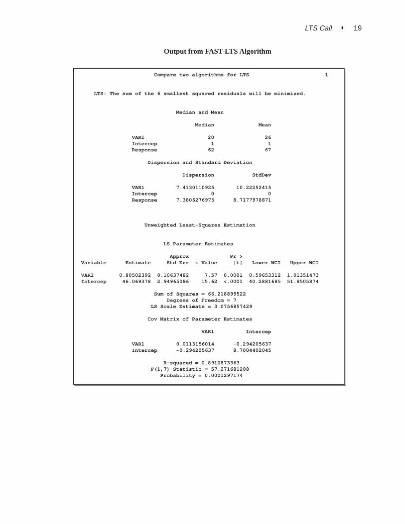
LTS Call � 19

Output from FAST-LTS Algorithm


LTS: The sum of the 6 smallest squared residuals will be minimized.

Median and Mean

Median Mean

VAR1 20 26Intercep 1 1Response 62 67

Dispersion and Standard Deviation

Dispersion StdDev

VAR1 7.4130110925 10.22252415Intercep 0 0Response 7.3806276975 8.7177978871

Unweighted Least-Squares Estimation

LS Parameter Estimates


VAR1 0.80502392 0.10637482 7.57 0.0001 0.59653312 1.01351473Intercep 46.069378 2.94965086 15.62 <.0001 40.2881685 51.8505874

Sum of Squares = 66.218899522Degrees of Freedom = 7

LS Scale Estimate = 3.0756857429


VAR1 Intercep

VAR1 0.0113156014 -0.294205637Intercep -0.294205637 8.7004402045

R-squared = 0.8910873363F(1,7) Statistic = 57.271681208

Probability = 0.0001297174



LS Residuals


1 80.000000 79.880383 0.119617 0.0388912 80.000000 75.855263 4.144737 1.3475813 75.000000 75.855263 -0.855263 -0.2780724 62.000000 68.610048 -6.610048 -2.1491305 62.000000 60.559809 1.440191 0.4682516 62.000000 60.559809 1.440191 0.4682517 62.000000 61.364833 0.635167 0.2065128 62.000000 62.169856 -0.169856 -0.0552269 58.000000 58.144737 -0.144737 -0.047058



-6.610047847 -0.512559809 0.1196172249

Mean 3rd Qu. MaxRes

-2.36848E-15 1.0376794258 4.1447368421

(no change)------------------------------------------------------------------------------------

Least Trimmed Squares (LTS) Method

The (at most) 10 Best Estimates

Objective Value [1]: 0.0428203092


VAR1 Intercep

0.7521545304 0.1250675364



VAR1 Intercep

0.7773132092 0.0679381212


LTS Call � 21



VAR1 Intercep

0.7857569344 0.0875053435



VAR1 Intercep

0.7454450208 0.1033087106



VAR1 Intercep

0.987904817 0.1606655488



VAR1 Intercep

0.1926222834 -0.081665104

Objective Value [7]: 1.797693E308

(added)-----------------------------------------------------------------------------------

Least Trimmed Squares (LTS) MethodMinimizing Sum of 6 Smallest Squared Residuals.

Highest Possible Breakdown Value = 44.44 %Selection of All 36 Subsets of 2 Cases Out of 9

Among 36 subsets 2 are singular.



The best half of the entire data set obtained after full iteration consists ofthe cases:

1 3 5 6 7 8


VAR1 Intercep

0.7488687783 47.945701357

LTS Objective Function = 0.6235087791

Preliminary LTS Scale = 1.1892734341

Robust R Squared = 0.819730444

Final LTS Scale = 0.8627851118

LTS Residuals


1 80.000000 79.398190 0.601810 0.6975202 80.000000 75.653846 4.346154 5.0373543 75.000000 75.653846 -0.653846 -0.7578324 62.000000 68.914027 -6.914027 -8.0136145 62.000000 61.425339 0.574661 0.6660536 62.000000 61.425339 0.574661 0.6660537 62.000000 62.174208 -0.174208 -0.2019148 62.000000 62.923077 -0.923077 -1.0698809 58.000000 59.178733 -1.178733 -1.366195



-6.914027149 -1.050904977 -0.174208145

Mean 3rd Qu. MaxRes

-0.416289593 0.5746606335 4.3461538462

(changed)------------------------------------------------------------------------------------

LTS Call � 23


Weighted Least-Squares Estimation

RLS Parameter Estimates Based on LTS


VAR1 0.76455907 0.03125286 24.46 <.0001 0.70330458 0.82581356Intercep 47.3985025 0.815574 58.12 <.0001 45.8000068 48.9969982

Weighted Sum of Squares = 3.3544093178Degrees of Freedom = 5

RLS Scale Estimate = 0.819073784


VAR1 Intercep

VAR1 0.0009767415 -0.02358133Intercep -0.02358133 0.6651609492

Weighted R-squared = 0.9917145853F(1,5) Statistic = 598.47009637

Probability = 2.1279132E-6There are 7 points with nonzero weight.

Average Weight = 0.7777777778

Weighted LS Residuals

N Observed Estimated Residual Res / S Weight

1 80.000000 79.509983 0.490017 0.598257 1.0000002 80.000000 75.687188 4.312812 5.265474 03 75.000000 75.687188 -0.687188 -0.838982 1.0000004 62.000000 68.806156 -6.806156 -8.309577 05 62.000000 61.160566 0.839434 1.024858 1.0000006 62.000000 61.160566 0.839434 1.024858 1.0000007 62.000000 61.925125 0.074875 0.091414 1.0000008 62.000000 62.689684 -0.689684 -0.842029 1.0000009 58.000000 58.866889 -0.866889 -1.058377 1.000000



-6.806156406 -0.77828619 0.074875208

Mean 3rd Qu. MaxRes

-0.27703827 0.6647254576 4.31281198

The run has been executed successfully.

(no change)------------------------------------------------------------------------------------



sc is 636

27

0.62350881.18927340.86278510.8197304

1.879.

0.81907383.35440930.9917146

598.4701......

coef is 0.7488688 47.9457010.7645591 47.3985020.0312529 0.81557424.463648 58.116742.1279E-6 2.8538E-80.7033046 45.8000070.8258136 48.996998

. .

(changed)------------------------------------------------------------------------------------

MCD Call

finds the minimum covariance determinant estimator

CALL MCD( sc, coef, dist, opt, x);

The MCD call is the robust (resistant) estimation of multivariate location and scatter,defined by minimizing the determinant of the covariance matrix computed fromhpoints. The algorithm for the MCD subroutine is based on the FAST-MCD algorithmgiven by Rousseeuw and Van Driessen (1999).

The MCD subroutine computes the minimum covariance determinant estimator.These robust locations and covariance matrices can be used to detect multivariateoutliers and leverage points. For this purpose, the MCD subroutine provides a tableof robust distances.

In the following discussion,N is the number of observations andn is the number ofregressors. The inputs to the MCD subroutine are as follows:

opt refers to an options vector with the following components (missing values

MCD Call � 25

are treated as default values):

opt[1] specifies the amount of printed output. Higher option values re-quest additional output and include the output of lower values.

opt[1]=0 prints no output except error messages.opt[1]=1 prints most of the output.opt[1]=2 additionally prints case numbers of the observations in

the best subset and some basic history of the optimiza-tion process.

opt[1]=3 additionally prints how many subsets result in singularlinear systems.

The default isopt[1]=0.

opt[2] specifies whether the classical, initial, and final robust covariancematrices are printed. The default isopt[2]=0. Note that the finalrobust covariance matrix is always returned incoef.

opt[3] specifies whether the classical, initial, and final robust correlationmatrices are printed or returned:

opt[3]=0 does not return or print.opt[3]=1 prints the robust correlation matrix.opt[3]=2 returns the final robust correlation matrix incoef.opt[3]=3 prints and returns the final robust correlation matrix.

opt[4] specifies the quantileh used in the objective function. The defaultis opt[5]= h =

�N+n+1

2

�. If the value ofh is specified outside

the rangeN2 + 1 � h � 3N4 + n+1

4 , it is reset to the closestboundary of this region.

opt[5] specifies the numberNRep of subset generations. This option isthe same as described for the LTS subroutines. Due to computertime restrictions, not all subset combinations can be inspected forlarger values ofN andn.

Whenopt[5] is zero or missing:

If N > 600, construct up to five disjoint random subsets withsizes as equal as possible, but not to exceed 300. Inside each sub-set, choose500=5 = 100 subset combinations ofn observations.

If N < 600, the number of subsets is taken from the followingtable.

n 1 2 3 4 5 6 7 8 9 10Nlower 500 50 22 17 15 14 0 0 0 0

n 11 12 13 14 15Nlower 0 0 0 0 0

If the number of cases (observations)N is smaller thanNlower,then all possible subsets are used; otherwise, 500 subsets are cho-


sen randomly. This means that an exhaustive search is performedfor opt[5]=�1. If N is larger thanNupper, a note is printed in thelog file indicating how many subsets exist.

x refers to anN � n matrixX of regressors.

Missing values are not permitted inx. Missing values inopt cause the default valueto be used.

The MCD subroutine returns the following values:

sc is a column vector containing the following scalar information:

sc[1] the quantileh used in the objective function

sc[2] number of subsets generated

sc[3] number of subsets with singular linear systems

sc[4] number of nonzero weightswi

sc[5] lowest value of the objective functionFMCD attained (smallestdeterminant)

sc[6] Mahalanobis-like distance used in the computation of the lowestvalue of the objective functionFMCD

sc[7] the cutoff value used for the outlier decision

coef is a matrix withn columns containing the following results in its rows:

coef[1] location of ellipsoid center

coef[2] eigenvalues of final robust scatter matrix

coef[3:2+n] the final robust scatter matrix foropt[2]=1 oropt[2]=3

coef[2+n+1:2+2n] the final robust correlation matrix foropt[3]=1 oropt[3]=3

dist is a matrix withN columns containing the following results in its rows:

dist[1] Mahalanobis distances

dist[2] robust distances based on the final estimates

dist[3] weights (=1 for small, =0 for large robust distances)

ExampleConsider Brownlee’s (1965) stackloss data used in the example for the MVE subrou-tine.

ForN = 21 andn = 4 (three explanatory variables including intercept), you obtaina total of 5,985 different subsets of 4 observations out of 21. If you decide not tospecifyoptn[5] , the MCD algorithm chooses500 random sample subsets:

MCD Call � 27

/* X1 X2 X3 Y Stackloss data */aa = { 1 80 27 89 42,

1 80 27 88 37,1 75 25 90 37,1 62 24 87 28,1 62 22 87 18,1 62 23 87 18,1 62 24 93 19,1 62 24 93 20,1 58 23 87 15,1 58 18 80 14,1 58 18 89 14,1 58 17 88 13,1 58 18 82 11,1 58 19 93 12,1 50 18 89 8,1 50 18 86 7,1 50 19 72 8,1 50 19 79 8,1 50 20 80 9,1 56 20 82 15,1 70 20 91 15 };

a = aa[,2:4];optn = j(8,1,.);optn[1]= 2; /* ipri */optn[2]= 1; /* pcov: print COV */optn[3]= 1; /* pcor: print CORR */

CALL MCD(sc,xmcd,dist,optn,a);

The first part of the output of this program is a summary of the MCD algorithm andthe finalh points selected:

Fast MCD by Rousseeuw and Van Driessen

Number of Variables 3Number of Observations 21Default Value for h 12Specified Value for h 12Breakdown Value 42.86- Highest Possible Breakdown Value -

The best half of the entire data set obtained after full iterationconsists of the cases:

4 5 6 7 8 9 10 11 12 13 14 20

The second part of the output is the MCD estimators of the location, scatter matrix,and correlation matrix:


MCD Location Estimate

VAR1 VAR2 VAR3

59.5 20.833333333 87.333333333Average of 12 Selected Points

MCD Scatter Matrix Estimate

VAR1 VAR2 VAR3

VAR1 5.1818181818 4.8181818182 4.7272727273VAR2 4.8181818182 7.6060606061 5.0606060606VAR3 4.7272727273 5.0606060606 19.151515152

Determinant = 238.07387929Covariance Matrix of 12 Selected Points

MCD Correlation Matrix

VAR1 VAR2 VAR3

VAR1 1 0.7674714142 0.4745347313VAR2 0.7674714142 1 0.4192963398VAR3 0.4745347313 0.4192963398 1

The MCD scatter matrix is multiplied by a factor to make itconsistent when all the data come from a single

Gaussian distribution.

Consistent Scatter Matrix

VAR1 VAR2 VAR3

VAR1 8.6578437815 8.0502757968 7.8983838007VAR2 8.0502757968 12.708297013 8.4553211199VAR3 7.8983838007 8.4553211199 31.998580526

Determinant = 397.77668436

The final output presents a table containing the classical Mahalanobis distances, therobust distances, and the weights identifying the outlying observations (that is, lever-age points when explainingy with these three regressor variables):

Classical Distances and Robust (Rousseeuw) DistancesUnsquared Mahalanobis Distance and

Unsquared Rousseeuw Distance of Each ObservationMahalanobis Robust

N Distances Distances Weight

1 2.253603 12.173282 02 2.324745 12.255677 03 1.593712 9.263990 04 1.271898 1.401368 1.000000

VARMACOV Call � 29

5 0.303357 1.420020 1.0000006 0.772895 1.291188 1.0000007 1.852661 1.460370 1.0000008 1.852661 1.460370 1.0000009 1.360622 2.120590 1.000000

10 1.745997 1.809708 1.00000011 1.465702 1.362278 1.00000012 1.841504 1.667437 1.00000013 1.482649 1.416724 1.00000014 1.778785 1.988240 1.00000015 1.690241 5.874858 016 1.291934 5.606157 017 2.700016 6.133319 018 1.503155 5.760432 019 1.593221 6.156248 020 0.807054 2.172300 1.00000021 2.176761 7.622769 0

Robust distances are based on reweighted estimates.

The cutoff value is the square root of the 0.975 quantileof the chi square distribution with 3 degrees of freedom.

Points whose robust distance exceeds 3.0575159206 havereceived a zero weight in the last column above.

There were 9 such points in the data.These may include boundary cases.

Only points whose robust distance is substantially largerthan the cutoff should be considered outliers.

Multivariate Time Series Analysis

These are the new functions for the creation and analysis of multivariate time series:

VARMACOV Call

computes the theoretical cross-covariance matrices for a stationaryVARMA( p; q) model

CALL VARMACOV( cov, phi, theta, sigma <, p, q, lag> );

The inputs to the VARMACOV subroutine are as follows:

phi specifies akmp � k matrix, �, containing the autoregressive coefficientmatrices, wheremp is the number of elements in the subset of the AR orderandk � 2 is the number of variables. All the roots ofj�(B)j = 0 shouldbe greater than one in absolute value, where�(B) is the finite order matrixpolynomial in the backshift operatorB, such thatBjyt = yt�j . You must


specify eitherphi or theta.

theta specifies akmq � k matrix containing the moving-average coefficient ma-trices, wheremq is the number of the elements in the subset of the MAorder. You must specify eitherphi or theta.

sigma specifies ak�k symmetric positive-definite covariance matrix of the inno-vation series. Ifsigmais not specified, then an identity matrix is used.

p specifies the subset of the AR order. The quantitymp is defined as

mp = nrow(phi)=ncol(phi)

wherenrow(phi) is the number of rows of the matrixphi andncol(phi) isthe number of columns of the matrixphi.

If you do not specifyp, the default subset isp= f1; 2; : : : ;mpg.

For example, consider a four-dimensional vector time series, andphi is a4 � 4 matrix. If you specifyp=1 (the default, sincemp = 4=4 = 1), theVARMACOV subroutine computes the theoretical cross-covariance matri-ces of VAR(1) asyt = �yt�1 + �t:

If you specify p=2, the VARMACOV subroutine computes the cross-covariance matrices of VAR(2) asyt = �yt�2 + �t:

Let phi = [�0

1; �0

2]0 be an8 � 4 matrix. If you specifyp= f1; 3g,

the VARMACOV subroutine computes the cross-covariance matrices ofVAR(3) asyt = �1yt�1 +�2yt�3 + �t: If you do not specifyp, the VAR-MACOV subroutine computes the cross-covariance matrices of VAR(2) asyt = �1yt�1 +�2yt�2 + �t:

q specifies the subset of the MA order. The quantitymq is defined as

mq = nrow(theta)=ncol(theta)

wherenrow(theta)is the number of rows of matrixthetaandncol(theta)isthe number of columns of matrixtheta.

If you do not specifyq, the default subset isq= f1; 2; : : : ;mqg.

The usage ofq is the same as that ofp.

lag specifies the length of lags, which must be a positive number. Iflag = h,the VARMACOV computes the cross-covariance matrices from lag zero tolagh. By default,lag = 12.

The VARMACOV subroutine returns the following value:

cov is a k(lag + 1) � k matrix that contains the theoretical cross-covariancematrices of the VARMA(p; q) model.

To compute the cross-covariance matrices of a bivariate (k = 2) VARMA(1,1) model

yt = �yt�1 + �t ��t�1

VARMALIK Call � 31

where

� =

�1:2 �0:50:6 0:3

�� =

��0:6 0:30:3 0:6

�� =

�1:0 0:50:5 1:25

�

you can specify

phi = { 1.2 -0.5, 0.6 0.3 };theta= {-0.6 0.3, 0.3 0.6 };sigma= { 1.0 0.5, 0.5 1.25};call varmacov(cov, phi, theta, sigma) lag=5;

VARMALIK Call

computes the log-likelihood function for a VARMA(p; q) model

CALL VARMALIK( lnl, series, phi, theta, sigma <, p, q, opt> );

The inputs to the VARMALIK subroutine are as follows:

series specifies ann� k matrix containing the vector time series (assuming meanzero), wheren is the number of observations andk � 2 is the number ofvariables.

phi specifies akmp � k matrix containing the autoregressive coefficient matri-ces, wheremp is the number of the elements in the subset of the AR order.You must specify eitherphi or theta.


sigma specifies ak � k covariance matrix of the innovation series. If you do notspecifysigma, an identity matrix wis used.

p specifies the subset of the AR order. See the VARMACOV subroutine.

q specifies the subset of the MA order. See the VARMACOV subroutine.

opt specifies the method of computing the log-likelihood function:

opt=0 requests the multivariate innovations algorithm. This algorithmrequires that the time series is stationary and does not containmissing observations.

opt=1 requests the conditional log-likelihood function. This algorithmrequires that the number of the observations in the time seriesmust be greater thanp+q and that the series does not containmissing observations.

opt=2 requests the Kalman filtering algorithm. This is the default and isused if the required conditions inopt=0 andopt=1 are not satis-fied.


The VARMALIK subroutine returns the following value:

lnl is a 3 � 1 matrix containing the log-likelihood function, the sum of logdeterminant of the innovation variance, and the weighted sum of squares ofresiduals. The log-likelihood function is computed as�0:5� (the sum oflast two terms).

The optionsopt=0andopt=2are equivalent for stationary time series without missingvalues. Settingopt=0 is useful for a small number of the observations and a highorder ofp andq; opt=1 is useful for a high order ofp andq; opt=2 is useful for a loworder ofp andq, or for missing values in the observations.

To compute the log-likelihood function of a bivariate (k = 2) VARMA(1,1) model

yt = �yt�1 + �t ��t�1

where

� =

�1:2 �0:50:6 0:3

�� =

��0:6 0:30:3 0:6

�� =

�1:0 0:50:5 1:25

�

you can specify

phi = { 1.2 -0.5, 0.6 0.3 };theta= {-0.6 0.3, 0.3 0.6 };sigma= { 1.0 0.5, 0.5 1.25};call varmasim(yt, phi, theta) sigma=sigma;call varmalik(lnl, yt, phi, theta, sigma);

VARMASIM Call

generates a VARMA(p,q) time series

CALL VARMASIM( series, phi, theta, mu, sigma, n <, p, q, initial, seed>);

The inputs to the VARMASIM subroutine are as follows:

phi specifies akmp � k matrix containing the autoregressive coefficient matri-ces, wheremp is the number of the elements in the subset of the AR orderandk � 2 is the number of variables. You must specify eitherphi or theta.


mu specifies ak� 1 (or 1�k) mean vector of the series. Ifmuis not specified,a zero vector is used.

sigma specifies ak� k covariance matrix of the innovation series. Ifsigmais notspecified, an identity matrix is used.

VNORMAL Call � 33

n specifies the length of the series. Ifn is not specified,n = 100 is used.



initial specifies the initial values of random variables. Ifinitial = a0, theny�p+1; : : : ;y0 and ��q+1; : : : ; �0 all take the same valuea0. If the ini-tial option is not specified, the initial values are estimated for the stationaryvector time series; the initial values are assumed as zero for the nonstation-ary vector time series.

seed specifies the random number seed. See the VNORMAL subroutine.

The VARMASIM subroutine returns the following value:

series is ann�k matrix containing the generated VARMA(p; q) time series. Wheneither theinitial option is specified or zero initial values are used, theseinitial values are not included inseries.

To generate a bivariate (k = 2) stationary VARMA(1,1) time series

yt � � = �(yt�1 � �) + �t ��t�1

where

� =

�1:2 �0:50:6 0:3

�� =

��0:6 0:30:3 0:6

�� =

�1020

�� =

�1:0 0:50:5 1:25

�

you can specify

phi = { 1.2 -0.5, 0.6 0.3 };theta= {-0.6 0.3, 0.3 0.6 };mu = { 10, 20 };sigma= { 1.0 0.5, 0.5 1.25};call varmasim(yt, phi, theta, mu, sigma, 100);

To generate a bivariate (k = 2) nonstationary VARMA(1,1) time series with the same�, �, and� in the previous example and the AR coefficient

� =

�1:0 00 0:3

�

you can specify

phi = { 1.0 0.0, 0.0 0.3 };call varmasim(yt, phi, theta, mu, sigma, 100) initial=3;


VNORMAL Call

generates a multivariate normal random series

CALL VNORMAL( series, mu, sigma, n <, seed>);

The inputs to the VNORMAL subroutine are as follows:

mu specifies ak � 1 (or 1 � k) mean vector, wherek � 2 is the number ofvariables. You must specify eithermuor sigma. If mu is not specified, azero vector is used.

sigma specifies ak�k symmetric positive-definite covariance matrix. By default,sigmais an identity matrix with dimensionk. You must specify eithermuor sigma. If sigmais not specified, an identity matrix is used.

n specifies the length of the series. Ifn is not specified,n = 100 is used.

seed specifies the random number seed. If it is not supplied, the system clock isused to generate the seed. If it is negative, then the absolute value is used asthe starting seed; otherwise, subsequent calls ignore the value ofseedanduse the last seed generated internally.

The VNORMAL subroutine returns the following value:

series is ann� k matrix that contains the generated normal random series.

To generate a bivariate (k = 2) normal random series with mean� and covariancematrix�, where

� =

�1020

�and � =

�1:0 0:50:5 1:25

�

you can specify

mu = { 10, 20 };sigma= { 1.0 0.5, 0.5 1.25};call vnormal(et, mu, sigma, 100);

VTSROOT Call

calculates the characteristic roots of the model from AR and MA characteristicfunctions

CALL VTSROOT( root, phi, theta<, p, q>);

The inputs to the VTSROOT subroutine are as follows:

VTSROOT Call � 35

phi specifies akmp � k matrix containing the autoregressive coefficient matri-ces, wheremp is the number of the elements in the subset of the AR orderandk � 2 is the number of variables. You must specify eitherphi or theta.




The VTSROOT subroutine returns the following value:

root is a k(pmax + qmax) � 5 matrix, wherepmax is the maximum order ofthe AR characteristic function andqmax is the maximum order of the MAcharacteristic function. The firstkpmax rows refer to the results of the ARcharacteristic function; the lastkqmax rows refer to the results of the MAcharacteristic function.

The first column contains the real parts,x, of eigenvalues of companion ma-trix associated with the AR(pmax) or MA(qmax) characteristic function; thesecond column contains the imaginary parts,y, of the eigenvalues; the thirdcolumn contains the moduli of the eigenvalues,

px2 + y2; the fourth col-

umn contains the arguments (arctan(y=x)) of the eigenvalues, measured inradians from the positive real axis. The fifth column contains the argumentsexpressed in degrees rather than radians.

To compute the roots of the characteristic functions,�(B) = I � �B and�(B) =I ��B, whereI is an identity matrix with dimension 2 and

� =

�1:2 �0:50:6 0:3

�� =

��0:6 0:30:3 0:6

�

you can specify

phi = { 1.2 -0.5, 0.6 0.3 };theta= {-0.6 0.3, 0.3 0.6 };call vtsroot(root, phi, theta);


References

Brownlee, K.A. (1965),Statistical Theory and Methodology in Science and Engi-neering, New York: John Wiley & Sons, Inc.

Rousseeuw, P.J. (1984), “Least Median of Squares Regression,”Journal of the Amer-ican Statistical Association, 79, 871–880.

Rousseeuw, P.J. and Hubert, M. (1997), “Recent Developments in PROGRESS,”L1-StatisticalProcedures and Related Topics, ed. by Y. Dodge, IMS LectureNotes, Monograph Series, No. 31, 201–214.

Rousseeuw, P.J. and Leroy, A.M. (1987),Robust Regression and Outlier Detection,New York: John Wiley & Sons, Inc.

Rousseeuw, P.J. and Van Driessen, K. (1998), “Computing LTS Regression for LargeData Sets,” Technical Report, University of Antwerp, submitted.

Rousseeuw, P.J. and Van Driessen, K. (1999), “A Fast Algorithm for the MinimumCovariance Determinant Estimator,”Technometrics, 41, 212–223.

Subject Index

CCONVEXIT function

calculating convexity of noncontingent cash flows,3

DDURATION function

calculating modified duration of noncontingentcash flows, 4

Fforward rates, 5

LLTS call

performs robust regression, 10

MMCD call, 24

PPV function

calculating present value, 6

RRATES function

converting interest rates, 7

SSPOT function

calculating spot rates, 8

VVARMACOV Call

computing cross-covariance matrices, 29VARMALIK Call

computing log-likelihood function, 31VARMASIM Call

generating VARMA(p,q) time series, 32VNORMAL Call

generating multivariate normal random series, 34VTSROOT Call

calculating characteristic roots, 34

YYIELD function

calculating yield-to-maturity of a cash-flow stream,

9

38 � Subject Index

Syntax Index

CCONVEXIT function, 3

DDURATION function, 4

FFORWARD function, 5

LLTS call, 10

MMCD call, 24

PPV function, 6

RRATES function, 7

SSPOT function, 8

VVARMACOV Call, 29VARMALIK Call, 31VARMASIM Call, 32VNORMAL Call, 34VTSROOT Call, 34

YYIELD function, 9

Your Turn

If you have comments or suggestions about SAS/IML® Software: Changes andEnhancements, Release 8.1, please send them to us on a photocopy of this page or sendus electronic mail.

For comments about this book, please return the photocopy toSAS InstitutePublications DivisionSAS Campus DriveCary, NC 27513email: [email protected]

For suggestions about the software, please return the photocopy toSAS InstituteTechnical Support DivisionSAS Campus DriveCary, NC 27513email: [email protected]

Welcome * Bienvenue * Willkommen * Yohkoso * Bienvenido

SAS® Institute Publishing Is Easy to Reach

Visit our Web page located at www.sas.com/pubs

You will find product and service details, including

• sample chapters

• tables of contents

• author biographies

• book reviews

Learn about

• regional user-group conferences• trade-show sites and dates• authoring opportunities

• custom textbooks

Explore all the services that SAS Institute Publishing has to offer!

Your Listserv Subscription Automatically Brings the News to YouDo you want to be among the first to learn about the latest books and services available from SAS InstitutePublishing? Subscribe to our listserv newdocnews-l and, once each month, you will automatically receive adescription of the newest books and which environments or operating systems and SAS release(s) that each bookaddresses.

To subscribe,

1. Send an e-mail message to [email protected].

2. Leave the “Subject” line blank.

3. Use the following text for your message:

subscribe NEWDOCNEWS-L your-first-name your-last-name

For example: subscribe NEWDOCNEWS-L John Doe

Create Customized Textbooks Quickly, Easily, and Affordably

SelecText® offers instructors at U.S. colleges and universities a way to create custom textbooks for courses thatteach students how to use SAS software.

For more information, see our Web page at www.sas.com/selectext, or contact our SelecText coordinators bysending e-mail to [email protected].

You’re Invited to Publish with SAS Institute’s User Publishing ProgramIf you enjoy writing about SAS software and how to use it, the User Publishing Program at SAS Instituteoffers a variety of publishing options. We are actively recruiting authors to publish books, articles, and samplecode. Do you find the idea of writing a book or an article by yourself a little intimidating? Consider writing witha co-author. Keep in mind that you will receive complete editorial and publishing support, access to our users,technical advice and assistance, and competitive royalties. Please contact us for an author packet. E-mail us [email protected] or call 919-677-8000, then press 1-6479. See the SAS Institute Publishing Web page atwww.sas.com/pubs for complete information.

See Observations®, Our Online Technical JournalFeature articles from Observations®: The Technical Journal for SAS® Software Users are now available online atwww.sas.com/obs. Take a look at what your fellow SAS software users and SAS Institute experts have to tellyou.You may decide that you, too, have information to share. If you are interested in writing for Observations, sende-mail to [email protected] or call 919-677-8000, then press 1-6479.

Book Discount Offered at SAS Public Training Courses!When you attend one of our SAS Public Training Courses at any of our regional Training Centers in the U.S., youwill receive a 15% discount on book orders that you place during the course.Take advantage of this offer at thenext course you attend!

SAS InstituteSAS Campus DriveCary, NC 27513-2414Fax 919-677-4444

* Note: Customers outside the U.S. should contact their local SAS office.

E-mail: [email protected] page: www.sas.com/pubsTo order books, call Fulfillment Services at 800-727-3228*For other SAS Institute business, call 919-677-8000*

Documents

SAS/IML Software: Changes and Enhancements, … ® Software: Changes and Enhancements, Release 8.1 The correct bibliographic citation for this manual is as follows: SAS Institute Inc.,