Embed Size (px)
Citation preview

SAPIENZA Universita di Roma
Tesi di Dottorato in Matematica
Dirpersive equations in Quantum Mechanics
Autore: Luca Fanelli
Relatore: Prof. P. D’Ancona

Contents
Introduction 3
Chapter 1. Decay estimates for the magnetic Dirac and wave equations 91. Introduction 92. The self-adjointness of the perturbed operators 133. The limiting absorption principle 154. Resolvent Estimates 245. Proof of Theorem 1.1 316. Proof of Theorem 1.2 337. Proof of Theorem 1.3 358. An appendix on Lorentz spaces 37
Chapter 2. Strichartz estimates and Kato-smoothing effect 411. Introduction 412. Resolvent Estimates 453. Proof of the Strichartz Estimates 564. Strichartz estimates for the free flows: an Appendix 62
Chapter 3. Dispersion via wave operators 671. Introduction 672. The high energy analysis 713. Fourier properties of the Jost Functions 744. The low energy analysis 79
Chapter 4. Nonlinear Schrodinger equations 871. NLS with time dependent coefficients 872. Strichartz estimates 913. Reduction to a nonlinear Schrodinger equation 934. Conservation laws 935. L2 global well-posedness 966. H1 local well-posedness 997. Global H1 theory 1048. Blow-up threshold for weakly coupled NLS 1069. Global existence results 10810. Gagliardo-Nirenberg inequality 10911. Blow-up results 112
1
2 CONTENTS
12. On the blow-up threshold 114
Bibliography 117

Introduction
It is a remarkable fact that evolution equations with different algebraic structures havesolutions with similar behaviors; throughout the standard classification of Partial DifferentialEquations in hyperbolic, parabolic and elliptic, the class off dispersive equations is an inter-esting family, which presents some typical and characterizing phenomena.
Among the others, dispersive equations include the following ones:
• the Schrodinger equation
(0.1)
{iut(t, x) + ∆xu(t, x) = 0 in R× Rn
u(0, x) = f(x);
• the wave equation
(0.2)
utt(t, x)−∆xu(t, x) = 0 in R× Rn
u(0, x) = f(x)ut(0, x) = g(x);
• the Klein-Gordon equation
(0.3)
utt(t, x)−∆xu(t, x) + u(t, x) = 0 in R× Rn
u(0, x) = f(x)ut(0, x) = g(x);
• the Dirac equation
(0.4)
{iut(t, x) +Hu(t, x) = 0 in R× R3
u(0, x) = f(x).
For the Schrodinger equation, the unknown u : R1+n → C is a complex-valued function; for thewave and Klein-Gordon equations u : R1+n → R is real-valued. Finally, for the Dirac equation,the unknown u : R1+3 → C4 is a spinor-valued function. The Dirac operator H is defined by
(0.5) H = −i3∑
j=1
αj∂j + β,
where the coefficients αj , β ∈M4×4(C) are the standard Hermitian 4× 4 Dirac matrices, whichare explicitly defined by
(0.6) α1 =
0 0 0 10 0 1 00 1 0 01 0 0 0
, α2 =
0 0 0 −i0 0 i 00 −i 0 0i 0 0 0
, α3 =
0 0 1 00 0 0 −11 0 0 00 −1 0 0
,
3
4 INTRODUCTION
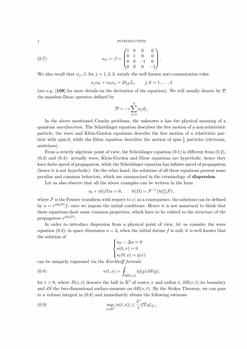
(0.7) α4 := β =
1 0 0 00 1 0 00 0 −1 00 0 0 −1
.
We also recall that αj , β, for j = 1, 2, 3, satisfy the well known anti-commutation rules
αjαk + αkαj = 2δjkI4, j, k = 1, . . . , 4
(see e.g. [108] for more details on the derivation of the equation). We will usually denote by Dthe massless Dirac operator defined by
D = −i3∑
j=1
αj∂j .
In the above mentioned Cauchy problems, the unknown u has the physical meaning of aquantum wavefunction. The Schrodinger equation describes the free motion of a non-relativisticparticle; the wave and Klein-Gordon equations describe the free motion of a relativistic par-ticle with spin-0, while the Dirac equation describes the motion of spin-1
2 particles (electrons,neutrinos).
From a strictly algebraic point of view, the Schrodinger equation (0.1) is different from (0.2),(0.3) and (0.4): actually wave, Klein-Gordon and Dirac equations are hyperbolic, hence theyhave finite speed of propagation, while the Schrodinger equation has infinite speed of propagation(hence it is not hyperbolic). On the other hand, the solutions of all these equations present somepeculiar and common behaviors, which are summarized in the terminology of dispersion.
Let us also observe that all the above examples can be written in the form
ut + ih(D)u = 0, h(D) = F−1 (h(ξ)F) ,
where F is the Fourier transform with respect to x; as a consequence, the solutions can be definedby u = eith(D)f , once we impose the initial conditions. Hence it is not unnatural to think thatthese equations show some common properties, which have to be related to the structure of thepropagators eith(D).
In order to introduce dispersion from a physical point of view, let us consider the waveequation (0.2); in space dimension n = 3, when the initial datum f is null, it is well known thatthe solution of
utt −∆u = 0u(0, x) = 0ut(0, x) = g(x)
can be uniquely expressed via the Kirchhoff formula
(0.8) u(t, x) =∫
∂B(x,t)− tg(y) dS(y),
for t > 0, where B(x, t) denotes the ball in R3 of center x and radius t, ∂B(x, t) its boundaryand dS the two-dimensional surface-measure on ∂B(x, t). By the Stokes Theorem, we can passto a volume integral in (0.8) and immediately obtain the following estimate
(0.9) supx∈R3
|u(t, x)| ≤ C
t‖∇g‖L1 ,

INTRODUCTION 5
for some C > 0 and for all times t > 0. Estimate (0.9) is interesting for large times, in fact itsays that the L∞-norm of u decays to 0 when t→ +∞. This is a very well known phenomenon,and it has a physical explanation. The energy
E(u, t) =12
∫R3
(|ut|2 + |∇u|2
)dx
is conserved under the wave flow, namely the identity
E(u, t) = E(u, 0)
holds for all times t ∈ R, on each solution u ∈ H1 of the equation. On the other hand, due to thefinite speed of propagation, if we start with a compactly supported initial datum, at each timet the solution is compactly supported (in space) in a bounded region whose diameter increasesas t. As a consequence, the solution tends to spread over this increasing region, and the energyconservation forces the intensity necessarily to decay.
This fact seems to be strictly related to the finite speed of propagation, but it is in fact (froma mathematical point of view) a consequence of the functional properties of the propagator ofthe equation.
For example, also the Schrodinger equation (0.1), which has infinite speed of propagation,has this property. The solution of (0.1) is uniquely determined by the propagator S(t) = eit∆,which is a unitary group of operators on L2, hence it conserves the mass (spacial L2-norm). Itcan be directly represented by its explicit convolution kernel, or by Fourier transforming withrespect to the space variable, we obtain the representation
(0.10) u(t, x) '∫
Rn
ei(t|ξ|2+x·ξ)f(ξ) dξ
for the solution of (0.1). The right hand side in (0.10) is an oscillatory integral (of the 1st kind),and by standard stationary phase methods (see e.g. [100]) it is possible to prove the dispersiveestimate
(0.11) supx∈Rn
|u(t, x)| ≤ C
tn/2‖f‖L1
(which is also immediate if we look at the kernel of eit∆). The last estimate is very similar to(0.9); in dimension n = 3 the Schrodinger solution decays faster than the wave one, with noloss of regularity with respect to the data. It is a fact that, if the initial datum is compactlysupported, the solution of the Schrodinger equation looses istantaneously this property, due tothe infinite speed of propagation; on the other hand, we can observe that most of the mass stayslocalized in a finite region, with increasing diameter. This, together with the L2-conservation,causes the same physical phenomenon which has been shown for the wave equation, and whichis described by estimate (0.11).
In both cases of wave and Schrodinger equation, for more general initial data, we can de-compose them into elementary wavepackets and observe that, during the evolution, the singlepackets travel independently with different speeds, but the same dispersive phenomena occurfor the total L∞-norm of the solution.

6 INTRODUCTION
In the last 30 years, dispersion has rapidly become one of the crucial tools in evolutionequations. This kind of physical phenomena can be summarized in a hierarchy of linear a prioriestimates for the solutions of the equations.
In this PhD thesis, we are interested in the above equations; we will focus our attention onthe following family of linear estimates:
• decay estimates• Strichartz estimates• Kato-smoothing estimates.
We give some examples, using the Schrodinger equation as a model.
0.1. Decay Estimates. Let us consider a solution u of (0.1); as we previously said, u satis-fies the L1−L∞ decay estimate (0.11). By interpolation between (0.1) and the L2-conservation,we immediately obtain the whole family of decay estimates for the Schrodinger equation
(0.12) ‖u(t)‖Lp ≤ Ct−n
2+n
p ‖f‖Lp′ , p ≥ 2,1p
+1p′
= 1.
Similar estimates hold for the wave, Klein-Gordon and Dirac equations, with a loss of derivativeson the initial data (see Chapter 1).
These estimates are well known and very interesting from a physical point of view. Theirinterest was historically motivated by the phenomenon itself; in the last years, once it wasdiscovered that decay estimates are basic to prove Strichartz estimates, they also became amathematical topic.
0.2. Strichartz Estimates. Strichartz estimates were introduced by R. Strichartz in [101],as a consequence of Fourier restriction theorems. In the fundamental papers [45], [47] by J.Ginibre and G. Velo, using the so called TT ∗ they proved Strichartz estimates as a consequenceof decay estimates. In the paper [66] by M. Keel and T. Tao the program was completed withthe proofs of the endpoint estimates.
The natural norms which are considered in this family of estimates are of mixed type, namelywe deal with Lp
tLqx-spaces. If u is the unique solution of the Schrodinger equation (0.1), then
the following estimates
(0.13) ‖u‖Lpt Lq
x= ‖eit∆f‖Lp
t Lqx≤ C‖f‖L2
hold for any couple (p, q) satisfying the Schrodinger admissibility condition2p = n
2 −nq
p ≥ 2 if n ≥ 3p > 2 if n = 2.
For the wave, Klein-Gordon and Dirac equation, similar estimates hold, with different admissi-bility conditions and different initial spaces (see the Appendix of Chapter 2).
Strichartz estimates represent the crucial instrument to perform fixed point arguments inthe study of nonlinear problems. One of the first examples of nonlinear application of Strichartzestimates was given in [46] for the nonlinear Schrodinger equation. Later, also for the nonlinearwave equation some critical problems were solved by this technique (see e.g. [52], [94]).

INTRODUCTION 7
0.3. Kato-smoothing and local smoothing estimates. The last family of estimateswe introduce are commonly referred to as smoothing effects. It is frequent for equations withinfinite speed of propagation that the solution is more regular then the initial data. The gainof derivatives, which is in fact related to the algebraic structure of the equations, is a veryinteresting fact, and is often a crucial improvement for nonlinear techniques.
The smoothing effect was discovered by T. Kato for the Kortweg-de Vries equation; for theSchrodinger equation, Kato and Yajima in [65] proved the well known inequality
(0.14) ‖〈x〉−12−|D|
12 eit∆f‖L2
t L2x≤ C‖f‖L2 ;
a stronger local version of the previous inequality (see the standard references [23], [109], [110])is the following:
(0.15) supR∈(0,+∞)
1R
∫ ∞
−∞
∫BR
∣∣∇ (eit∆f)∣∣2 dx dt ≤ C‖f‖H
12.
Here |D|12 = F−1(|ξ|
12F), F is the standard Fourier transform, BR is the ball of radius R
centered in 0, and H12 is the usual homogeneous Sobolev space with the norm
‖f‖H
12
= ‖|D|12 f‖L2 .
Both estimates (0.14) and (0.15) show that the unique solution of the free Schrodinger equationwith initial datum f gains half derivative in L2 with respect to f , if we look to a weighted L2
tL2x
norm.For the wave, Klein-Gordon and Dirac equations, we cannot expect a gain of derivatives on
the solutions, because of the finite speed of propagation; on the other hand, estimates whichare analogous to the previous ones for Schrodinger hold also for these equations, with the sameregularity for all times (see Chapter 2).
An example of application of Kato-smoothing-type estimates is given in Chapter 2, wherethey are a tool to prove Strichartz estimates.
0.4. Aim of the thesis and plan of the work. The aim of this PhD work was to studydispersive phenomena for some perturbations of the above mentioned equations. In particular,we are interested in:
• electromagnetic and electrostatic potentials (linear perturbations)• nonlinear perturbations.
When we deal with physical models in which particles interact with some external source, itis a fundamental problem to compare the asymptotic behavior of free and perturbed solutions.This is a physical motivation to investigate on dispersive estimates for equations with externalpotentials of electromagnetic type, which are usually represented by lower order terms in theequations.
From a mathematical point of view, it is clear that dispersive-type estimates have to beconsidered as a tool, more than a goal: they turn out to be crucial to prove existence anduniqueness results. In particular, the well-posedness problem for some nonlinear equations canbe easily solved by standard fixed point arguments in which Strichartz estimates are involved. In
8 INTRODUCTION
a sense, Strichartz estimates play the role which have the Sobolev embeddings in the nonlinearelliptic theory.
The first part of this thesis (Chapters 1,2,3) is devoted to linear equations with potentials.In Chapter 1 we prove some decay estimates for the wave and massless Dirac equations withmagnetic potentials (see also [31]), using functional techniques based on the Spectral Theoremand resolvent estimates. In Chapter 2, with similar techniques, we study Strichartz and Kato-smoothing estimates for Schrodinger, wave, Klein-Gordon, massless and massive Dirac equationswith magnetic potentials (see also [32]). Chapter 3 concludes the linear part of the work;here we present a different and indirect technique to prove linear dispersive estimates for 1DSchrodinger, wave and Klein-Gordon equations with an electric potential. It is based on themapping properties of the wave operators, which are at the core of Scattering Theory (see[30]). Chapter 4 completes the work, with two nonlinear applications. The first is a nonlinearSchrodinger equation with time dependent coefficients, possibly vanishing; we are interested inexistence and uniqueness results, and some Lorentz spaces version of Strichartz estimates arealso proved (see [38]). The second example is a system of two coupled nonlinear Schrodingerequations; here we prove existence, uniqueness and blow-up results, and we explicitly estimatea blow-up threshold for the the initial data (see also [40]).
Ringraziamenti e Dediche. Il mio primo ringraziamento va a Piero D’Ancona, per tuttoil tempo che mi ha dedicato, per la serieta e la portata del suo insegnamento e per essere statouna guida costante durante i quattro anni del mio dottorato.
Ringrazio tutti gli amici del Castelnuovo, per essermi stati, ognuno a modo suo, semprefamiliari e per aver reso questi anni indimenticabili.
Ringrazio la citta di Roma che mi ha ospitato; e chi, in modo gratuito e con il sorriso involto me l’ha insegnata e me l’ha fatta amare.
Un grazie speciale a mio padre, mia madre e mia sorella, che da lontano ed in silenzio, masempre presenti, hanno saputo rendere la mia vita piu semplice e piu bella.
Dedico questo lavoro al ricordo di Giulio Minervini. Fu il mio primo incontro in auladottorandi; di lui non dimentichero la risata contagiosa, l’umorismo caustico e l’insegnamentodell’ottimismo.

CHAPTER 1
Decay estimates for the magnetic Dirac and wave equations
1. Introduction
The first part of this thesis is devoted to the study of dispersive a priori estimates for solutionsof the perturbed equations. A very natural problem consists in extending the known estimatesfor the free equations to some typical perturbative equations coming out from physical models.In particular, we are interested to the case of electrostatic or electromagnetostatic potentials,for which some examples are given here and in the following chapters. In the present chapterwe treat Dirac and wave equations with electromagnetic potentials, and we prove some decayestimates for both the equations; the proofs of the main Theorem were given in [31].
Dispersive properties of evolution equations play a crucial role in the study of nonlinearproblems, and for this reason they have attracted a great deal of attention in recent years.In particular, for the Schrodinger and the wave equation a well established theory exists, see[47] and [66]. On the other hand, in the variable coefficient case the theory is very far fromcomplete. The simplest situtation is a perturbation with a term of order zero; this is alreadyvery interesting from the physical point of view (electrostatic potential). Several results areavailable for the equations
i∂tu−∆u+ V (x)u = 0, �u+ V (x)u = 0.
We cite among the others [17], [50], [49], [60], [84] [90] and the recent survey [92] for Schro-dinger; and [11], [12], [24], [33], [44] for the wave equation. We must also mention the waveoperator approach of Kato and Yajima (see [62], [5], [115], [116], [117]) which permits todeal with the above equations in a unified way, although under nonoptimal assumptions on thepotential in dimensions 1 and 3.
The next step in generality is a perturbation with a first order differential operator a(x) ·∇;from the physical point of view this corresponds to a magnetic potential. In this case only ahandful of results are available: Strichartz estimates for the 3D wave equation [25], provided thecoefficients are small and in the Schwartz class; and smoothing estimates for the 3D Schrodingerand wave operators [106]. The most general case of variable coefficients has been studied in[53], [88] and [97], where local Strichartz estimates have been proved, in various degrees ofcomplexity; see also [13].
In the present chapter, our main focus will be on the three dimensional wave equation withan electromagnetic potential
(1.1) utt − (∇+ iA(x))2u+B(x)u = 0, u : R× R3 → C,9

10 1. DECAY ESTIMATES FOR THE MAGNETIC DIRAC AND WAVE EQUATIONS
and the closely related massless Dirac system with a potential:
(1.2) iut −Du+ V (x)u = 0, u : R× R3 → C4.
Here A : R3 → R3, B : R3 → R, V (x) = V ∗(x) is a 4×4 complex matrix on R3, and the symbolD denotes the constant coefficient, elliptic, L2 selfadjoint operator
D =1i
3∑j=1
αk∂k,
where the Dirac matrices α1, α2, α3 have the following structure:
(1.3) α1 =
0 0 0 10 0 1 00 1 0 01 0 0 0
, α2 =
0 0 0 −i0 0 i 00 −i 0 0i 0 0 0
, α3 =
0 0 1 00 0 0 −11 0 0 00 −1 0 0
.
We neglect the physical constants (i.e., we set c = ~ = 1), and we consider the zero mass caseexclusively; the case of a positive mass, whose second order counterpart is the Klein-Gordonequation, has an additional term α4u with
(1.4) α4 =
1 0 0 00 1 0 00 0 −1 00 0 0 −1
.
The relation between massless Dirac and wave equation is readily explained: indeed, the Diracmatrices satisfy the commutation rules
α`αk + αkα` = 2δklI4
which imply immediatelyD2 = −∆I4,
where I4 is the 4×4 identity matrix. Thus we have the fundamental relation
(i∂t −D)(i∂t +D) = (∆− ∂2tt)I4,
which can be intepreted as follows: squaring the Dirac system produces a diagonal system ofwave equations (or, conversely: taking the square root of a wave equation produces a Diracsystem. According to the folklore, this was the route that led Dirac to his equation). When apotential is present in the Dirac system, the above reduction produces an electromagnetic waveequation in a natural way. A discussion of this can be found e.g. in [67] (Volume 4, Chapter 4);see also section 6 below.
Our goal here is to establish the decay rate of the spatial L∞ norm of the solution, withminimal assumptions on the potentials. The expected decay rate is t−1, both for the waveequation and the Dirac system. Indeed, known results for hyperbolic systems (for constantcoefficients see e.g. [70], [73], and for C∞0 perturbations thereof see [61]) suggest a t−
n−12 decay
rate in n space dimensions.Before stating our first result we introduce some basic notations. Under the assumptions of
Theorem 1.1 below, the perturbed laplacian
(1.5) H := −(∇+ iA(x))2 +B(x),
1. INTRODUCTION 11
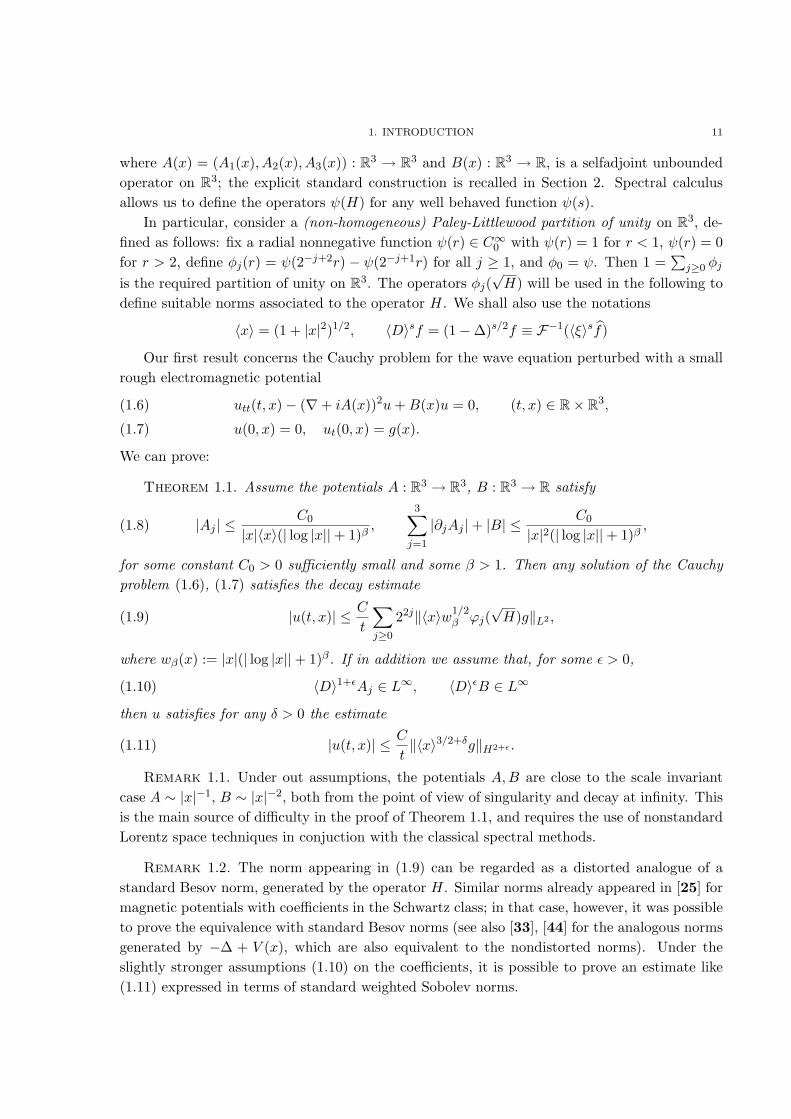
where A(x) = (A1(x), A2(x), A3(x)) : R3 → R3 and B(x) : R3 → R, is a selfadjoint unboundedoperator on R3; the explicit standard construction is recalled in Section 2. Spectral calculusallows us to define the operators ψ(H) for any well behaved function ψ(s).
In particular, consider a (non-homogeneous) Paley-Littlewood partition of unity on R3, de-fined as follows: fix a radial nonnegative function ψ(r) ∈ C∞0 with ψ(r) = 1 for r < 1, ψ(r) = 0for r > 2, define φj(r) = ψ(2−j+2r) − ψ(2−j+1r) for all j ≥ 1, and φ0 = ψ. Then 1 =
∑j≥0 φj
is the required partition of unity on R3. The operators φj(√H) will be used in the following to
define suitable norms associated to the operator H. We shall also use the notations
〈x〉 = (1 + |x|2)1/2, 〈D〉sf = (1−∆)s/2f ≡ F−1(〈ξ〉sf)
Our first result concerns the Cauchy problem for the wave equation perturbed with a smallrough electromagnetic potential
utt(t, x)− (∇+ iA(x))2u+B(x)u = 0, (t, x) ∈ R× R3,(1.6)
u(0, x) = 0, ut(0, x) = g(x).(1.7)
We can prove:
Theorem 1.1. Assume the potentials A : R3 → R3, B : R3 → R satisfy
(1.8) |Aj | ≤C0
|x|〈x〉(| log |x||+ 1)β,
3∑j=1
|∂jAj |+ |B| ≤ C0
|x|2(| log |x||+ 1)β,
for some constant C0 > 0 sufficiently small and some β > 1. Then any solution of the Cauchyproblem (1.6), (1.7) satisfies the decay estimate
(1.9) |u(t, x)| ≤ C
t
∑j≥0
22j‖〈x〉w1/2β ϕj(
√H)g‖L2 ,
where wβ(x) := |x|(| log |x||+ 1)β. If in addition we assume that, for some ε > 0,
(1.10) 〈D〉1+εAj ∈ L∞, 〈D〉εB ∈ L∞
then u satisfies for any δ > 0 the estimate
(1.11) |u(t, x)| ≤ C
t‖〈x〉3/2+δg‖H2+ε .
Remark 1.1. Under out assumptions, the potentials A,B are close to the scale invariantcase A ∼ |x|−1, B ∼ |x|−2, both from the point of view of singularity and decay at infinity. Thisis the main source of difficulty in the proof of Theorem 1.1, and requires the use of nonstandardLorentz space techniques in conjuction with the classical spectral methods.
Remark 1.2. The norm appearing in (1.9) can be regarded as a distorted analogue of astandard Besov norm, generated by the operator H. Similar norms already appeared in [25] formagnetic potentials with coefficients in the Schwartz class; in that case, however, it was possibleto prove the equivalence with standard Besov norms (see also [33], [44] for the analogous normsgenerated by −∆ + V (x), which are also equivalent to the nondistorted norms). Under theslightly stronger assumptions (1.10) on the coefficients, it is possible to prove an estimate like(1.11) expressed in terms of standard weighted Sobolev norms.
12 1. DECAY ESTIMATES FOR THE MAGNETIC DIRAC AND WAVE EQUATIONS
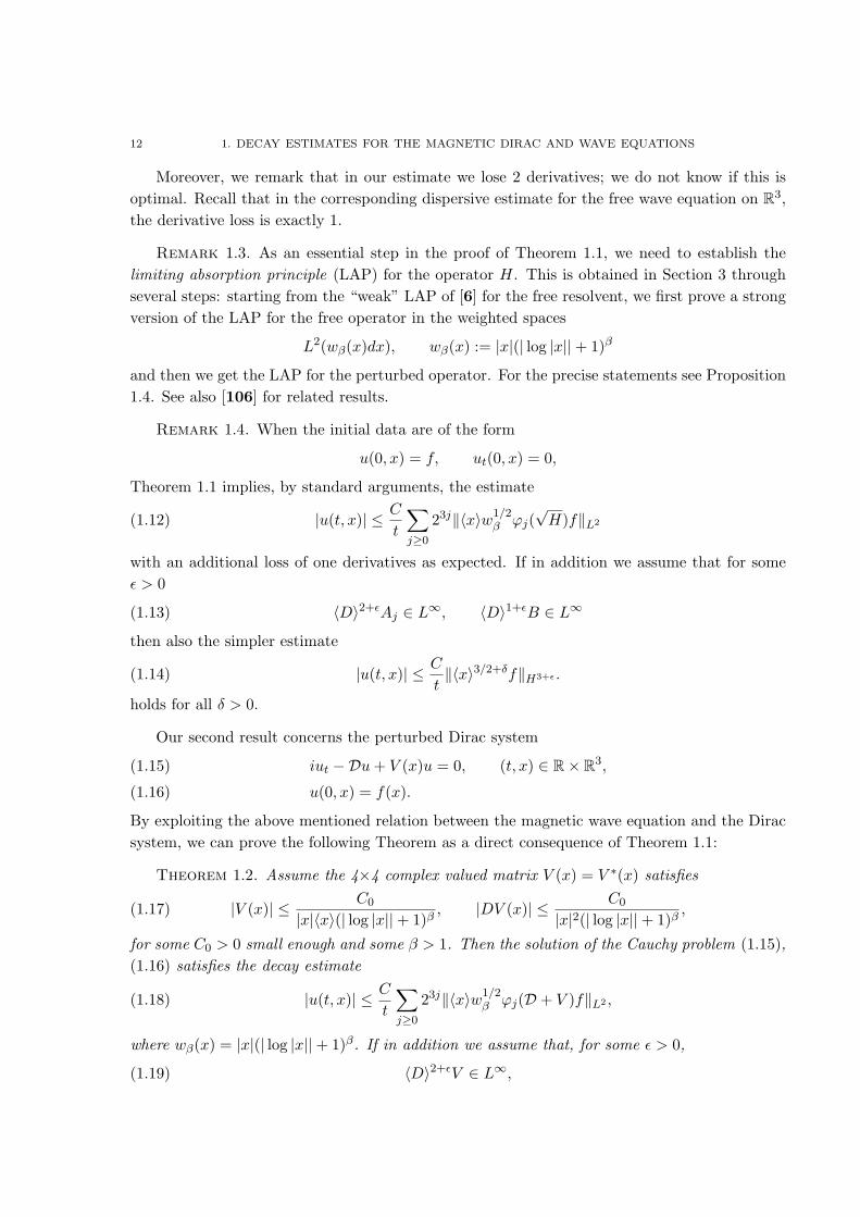
Moreover, we remark that in our estimate we lose 2 derivatives; we do not know if this isoptimal. Recall that in the corresponding dispersive estimate for the free wave equation on R3,the derivative loss is exactly 1.
Remark 1.3. As an essential step in the proof of Theorem 1.1, we need to establish thelimiting absorption principle (LAP) for the operator H. This is obtained in Section 3 throughseveral steps: starting from the “weak” LAP of [6] for the free resolvent, we first prove a strongversion of the LAP for the free operator in the weighted spaces
L2(wβ(x)dx), wβ(x) := |x|(| log |x||+ 1)β
and then we get the LAP for the perturbed operator. For the precise statements see Proposition1.4. See also [106] for related results.
Remark 1.4. When the initial data are of the form
u(0, x) = f, ut(0, x) = 0,
Theorem 1.1 implies, by standard arguments, the estimate
(1.12) |u(t, x)| ≤ C
t
∑j≥0
23j‖〈x〉w1/2β ϕj(
√H)f‖L2
with an additional loss of one derivatives as expected. If in addition we assume that for someε > 0
(1.13) 〈D〉2+εAj ∈ L∞, 〈D〉1+εB ∈ L∞
then also the simpler estimate
(1.14) |u(t, x)| ≤ C
t‖〈x〉3/2+δf‖H3+ε .
holds for all δ > 0.
Our second result concerns the perturbed Dirac system
iut −Du+ V (x)u = 0, (t, x) ∈ R× R3,(1.15)
u(0, x) = f(x).(1.16)
By exploiting the above mentioned relation between the magnetic wave equation and the Diracsystem, we can prove the following Theorem as a direct consequence of Theorem 1.1:
Theorem 1.2. Assume the 4×4 complex valued matrix V (x) = V ∗(x) satisfies
(1.17) |V (x)| ≤ C0
|x|〈x〉(| log |x||+ 1)β, |DV (x)| ≤ C0
|x|2(| log |x||+ 1)β,
for some C0 > 0 small enough and some β > 1. Then the solution of the Cauchy problem (1.15),(1.16) satisfies the decay estimate
(1.18) |u(t, x)| ≤ C
t
∑j≥0
23j‖〈x〉w1/2β ϕj(D + V )f‖L2 ,
where wβ(x) = |x|(| log |x||+ 1)β. If in addition we assume that, for some ε > 0,
(1.19) 〈D〉2+εV ∈ L∞,
2. THE SELF-ADJOINTNESS OF THE PERTURBED OPERATORS 13
then u satisfies for any δ > 0 the estimate
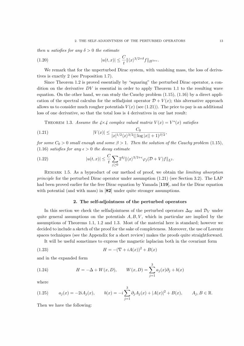
(1.20) |u(t, x)| ≤ C
t‖〈x〉3/2+δf‖H3+ε .
We remark that for the unperturbed Dirac system, with vanishing mass, the loss of deriva-tives is exactly 2 (see Proposition 1.7).
Since Theorem 1.2 is proved essentially by “squaring” the perturbed Dirac operator, a con-dition on the derivative DV is essential in order to apply Theorem 1.1 to the resulting waveequation. On the other hand, we can study the Cauchy problem (1.15), (1.16) by a direct appli-cation of the spectral calculus for the selfadjoint operator D + V (x); this alternative approachallows us to consider much rougher potentials V (x) (see (1.21)). The price to pay is an additionalloss of one derivative, so that the total loss is 4 derivatives in our last result:
Theorem 1.3. Assume the 4×4 complex valued matrix V (x) = V ∗(x) satisfies
(1.21) |V (x)| ≤ C0
|x|1/2〈x〉3/2(| log |x||+ 1)β/2,
for some C0 > 0 small enough and some β > 1. Then the solution of the Cauchy problem (1.15),(1.16) satisfies for any ε > 0 the decay estimate
(1.22) |u(t, x)| ≤ C
t
∑j≥0
24j‖〈x〉3/2+εϕj(D + V )f‖L2 .
Remark 1.5. As a byproduct of our method of proof, we obtain the limiting absorptionprinciple for the perturbed Dirac operator under assumption (1.21) (see Section 3.2). The LAPhad been proved earlier for the free Dirac equation by Yamada [119], and for the Dirac equationwith potential (and with mass) in [82] under quite stronger assumptions.
2. The self-adjointness of the perturbed operators
In this section we check the selfadjointness of the perturbed operators ∆W and DV underquite general assumptions on the potentials A,B, V , which in particular are implied by theassumptions of Theorems 1.1, 1.2 and 1.3. Most of the material here is standard; however wedecided to include a sketch of the proof for the sake of completeness. Moreover, the use of Lorentzspaces techniques (see the Appendix for a short review) makes the proofs quite straightforward.
It will be useful sometimes to express the magnetic laplacian both in the covariant form
(1.23) H = −(∇+ iA(x))2 +B(x)
and in the expanded form
(1.24) H = −∆ +W (x,D), W (x,D) =3∑
j=1
aj(x)∂j + b(x)
where
(1.25) aj(x) = −2iAj(x), b(x) = −i3∑
j=1
∂jAj(x) + |A(x)|2 +B(x), Aj , B ∈ R.
Then we have the following:
14 1. DECAY ESTIMATES FOR THE MAGNETIC DIRAC AND WAVE EQUATIONS
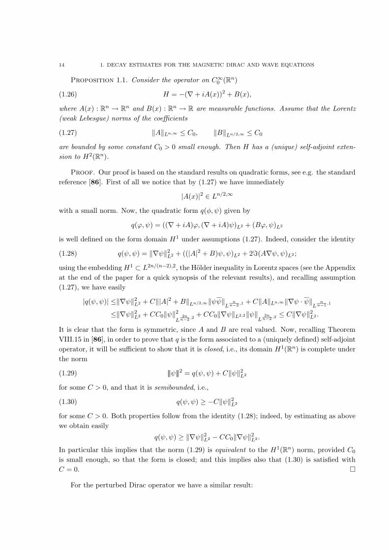
Proposition 1.1. Consider the operator on C∞0 (Rn)
(1.26) H = −(∇+ iA(x))2 +B(x),
where A(x) : Rn → Rn and B(x) : Rn → R are measurable functions. Assume that the Lorentz(weak Lebesgue) norms of the coefficients
(1.27) ‖A‖Ln,∞ ≤ C0, ‖B‖Ln/2,∞ ≤ C0
are bounded by some constant C0 > 0 small enough. Then H has a (unique) self-adjoint exten-sion to H2(Rn).
Proof. Our proof is based on the standard results on quadratic forms, see e.g. the standardreference [86]. First of all we notice that by (1.27) we have immediately
|A(x)|2 ∈ Ln/2,∞
with a small norm. Now, the quadratic form q(φ, ψ) given by
q(ϕ,ψ) = ((∇+ iA)ϕ, (∇+ iA)ψ)L2 + (Bϕ,ψ)L2
is well defined on the form domain H1 under assumptions (1.27). Indeed, consider the identity
(1.28) q(ψ,ψ) = ‖∇ψ‖2L2 + ((|A|2 +B)ψ,ψ)L2 + 2=(A∇ψ,ψ)L2 ;
using the embeddingH1 ⊂ L2n/(n−2),2, the Holder inequality in Lorentz spaces (see the Appendixat the end of the paper for a quick synopsis of the relevant results), and recalling assumption(1.27), we have easily
|q(ψ,ψ)| ≤‖∇ψ‖2L2 + C‖|A|2 +B‖Ln/2,∞‖ψψ‖
Ln
n−2 ,1 + C‖A‖Ln,∞‖∇ψ · ψ‖L
nn−1 ,1
≤‖∇ψ‖2L2 + CC0‖ψ‖2
L2n
n−2 ,2+ CC0‖∇ψ‖L2,2‖ψ‖
L2n
n−2 ,2 ≤ C‖∇ψ‖2L2 .
It is clear that the form is symmetric, since A and B are real valued. Now, recalling TheoremVIII.15 in [86], in order to prove that q is the form associated to a (uniquely defined) self-adjointoperator, it will be sufficient to show that it is closed, i.e., its domain H1(Rn) is complete underthe norm
(1.29) |||ψ|||2 = q(ψ,ψ) + C‖ψ‖2L2
for some C > 0, and that it is semibounded, i.e.,
(1.30) q(ψ,ψ) ≥ −C‖ψ‖2L2
for some C > 0. Both properties follow from the identity (1.28); indeed, by estimating as abovewe obtain easily
q(ψ,ψ) ≥ ‖∇ψ‖2L2 − CC0‖∇ψ‖2
L2 .
In particular this implies that the norm (1.29) is equivalent to the H1(Rn) norm, provided C0
is small enough, so that the form is closed; and this implies also that (1.30) is satisfied withC = 0. �
For the perturbed Dirac operator we have a similar result:

3. THE LIMITING ABSORPTION PRINCIPLE 15
Proposition 1.2. Let V (x) = V ∗(x) be a 4×4 complex valued matrix on R3. Assume that
(1.31) ‖V ‖L3,∞ ≤ C0,
for some C0 > 0 sufficiently small. Then the perturbed Dirac operator DV = D+V is self-adjointon H1(R3,C4).
Proof. The proof is analogous to the proof of Theorem 1.1. We define the quadratic formq : H1/2 ×H1/2 → C associated to the operator DV as
q(ϕ,ψ) := (Dϕ,ψ) + (V ϕ, ψ).
First we prove that the domain of q is H1/2. With the same arguments of the previous theoremwe estimate
|q(ϕ,ϕ)| ≤ ‖ϕ‖2H1/2 + C‖V ‖L3,∞‖ϕ2‖Ln/(n−1),1
≤ ‖ϕ‖2H1/2 + C‖V ‖L3,∞‖ϕ‖2
L2n/(n−1),2
≤ (1 + C‖V ‖L3,∞) ‖ϕ‖H1/2
(where we used the embedding H1/2 ⊂ L2n/(n−1),2). From this point on, the proof proceedsexactly as in Proposition 1.1 �
3. The limiting absorption principle
The essential tool in our proof will be the spectral theorem in the following version: givena selfadjoint (unbounded) operator A on L2 and a continuous bounded function f(λ) on R, theoperator f(A) can be defined as the L2 limit
(1.32) f(A)φ = − 1π· lim
ε↓0
∫f(λ)=R(λ+ iε)φdλ
for any φ ∈ L2. HereR(z) = (A−z)−1 denotes the resolvent operator of A (see e.g. [107]). Undersuitable assumptions on H, the limit operators R(λ± i0) = limε↓0R(λ± iε) are well defined asbounded operators in weighted L2 spaces; this is usually called the limiting absorption principle(see below for details). Thus we have also the simpler representation
(1.33) f(A)φ = − 1π·∫f(λ)=R(λ+ i0)φdλ.
Recalling the definition (1.25), consider now the operators
H = −∆ +W (x,D) ≡ −∆ +3∑
j=1
aj(x)∂j + b(x)
and
DV = D + V (x).
In Section 2 we proved that, under assumptions (1.27) on aj , b and V (x), both H and DV areselfadjoint operators on L2. In particular, the spectral formula (1.32) holds for both. We shalluse the following notations: the free resolvents will be written as
R0(z) = (−z −∆)−1, RD(z) = (−zI4 +D)−1
16 1. DECAY ESTIMATES FOR THE MAGNETIC DIRAC AND WAVE EQUATIONS
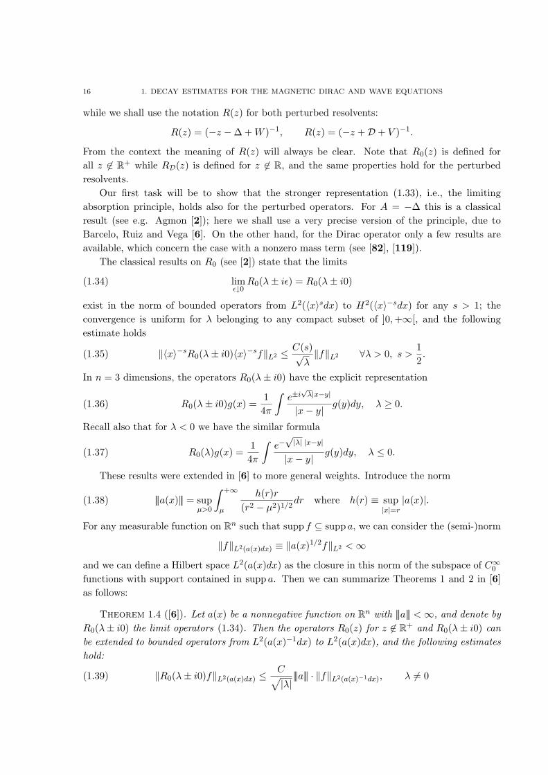
while we shall use the notation R(z) for both perturbed resolvents:
R(z) = (−z −∆ +W )−1, R(z) = (−z +D + V )−1.
From the context the meaning of R(z) will always be clear. Note that R0(z) is defined forall z 6∈ R+ while RD(z) is defined for z 6∈ R, and the same properties hold for the perturbedresolvents.
Our first task will be to show that the stronger representation (1.33), i.e., the limitingabsorption principle, holds also for the perturbed operators. For A = −∆ this is a classicalresult (see e.g. Agmon [2]); here we shall use a very precise version of the principle, due toBarcelo, Ruiz and Vega [6]. On the other hand, for the Dirac operator only a few results areavailable, which concern the case with a nonzero mass term (see [82], [119]).
The classical results on R0 (see [2]) state that the limits
(1.34) limε↓0
R0(λ± iε) = R0(λ± i0)
exist in the norm of bounded operators from L2(〈x〉sdx) to H2(〈x〉−sdx) for any s > 1; theconvergence is uniform for λ belonging to any compact subset of ]0,+∞[, and the followingestimate holds
(1.35) ‖〈x〉−sR0(λ± i0)〈x〉−sf‖L2 ≤C(s)√λ‖f‖L2 ∀λ > 0, s >
12.
In n = 3 dimensions, the operators R0(λ± i0) have the explicit representation
(1.36) R0(λ± i0)g(x) =14π
∫e±i
√λ|x−y|
|x− y|g(y)dy, λ ≥ 0.
Recall also that for λ < 0 we have the similar formula
(1.37) R0(λ)g(x) =14π
∫e−√|λ| |x−y|
|x− y|g(y)dy, λ ≤ 0.
These results were extended in [6] to more general weights. Introduce the norm
(1.38) |||a(x)||| = supµ>0
∫ +∞
µ
h(r)r(r2 − µ2)1/2
dr where h(r) ≡ sup|x|=r
|a(x)|.
For any measurable function on Rn such that supp f ⊆ supp a, we can consider the (semi-)norm
‖f‖L2(a(x)dx) ≡ ‖a(x)1/2f‖L2 <∞
and we can define a Hilbert space L2(a(x)dx) as the closure in this norm of the subspace of C∞0functions with support contained in supp a. Then we can summarize Theorems 1 and 2 in [6]as follows:
Theorem 1.4 ([6]). Let a(x) be a nonnegative function on Rn with |||a||| <∞, and denote byR0(λ± i0) the limit operators (1.34). Then the operators R0(z) for z 6∈ R+ and R0(λ± i0) canbe extended to bounded operators from L2(a(x)−1dx) to L2(a(x)dx), and the following estimateshold:
(1.39) ‖R0(λ± i0)f‖L2(a(x)dx) ≤C√|λ||||a||| · ‖f‖L2(a(x)−1dx), λ 6= 0

3. THE LIMITING ABSORPTION PRINCIPLE 17
(here of course R0(λ± i0) ≡ R0(λ) for λ < 0)
(1.40) ‖∇R0(λ± i0)f‖L2(a(x)dx) ≤ C|||a||| · ‖f‖L2(a(x)−1dx).
Moreover, the limiting absorption principle holds in the weak form: for all f, g ∈ L2(a(x)−1dx)
(1.41) limε↓0
(R0(λ± iε)f, g) = (R0(λ± i0)f, g).
Remark 1.6. It is not difficult to extend the estimates (1.39) and (1.40) to the whole complexplane. Indeed, fix two functions f, g ∈ C∞0 with support contained in supp a and consider onthe half plane
S = {z : =z > 0}the holomorphic function
(1.42) F (z) = z1/2(R0(z)f, g).
It is clear that F (z) is continuous on S up to the boundary, moreover it satisfies the estimate
(1.43) |F (x)| ≤ C|||a||| · ‖f‖L2(a(x)−1dx)‖g‖L2(a(x)−1dx)
on the boundary =z = 0, and finally it has a polynomial growth for |z| → +∞, as it easily followsfrom the explicit expression of R0(z) as a convolution operator (see [6]). By the Phragmen-Lindelof Theorem (see e.g. [100]) on the half plane we immediately obtain that estimate (1.43)holds on all of S. A similar argument can be applied in the lower half plane =z < 0. Inconclusion we obtain
(1.44) ‖R0(z)f‖L2(a(x)dx) ≤C√|z|
|||a||| · ‖f‖L2(a(x)−1dx)
for all f ∈ L2(a(x)−1dx) (see also part (ii) in Theorem 1, [6]). Notice that this estimate holdson the whole complex plane, in the sense that we apply it to R0(λ± i0) when z ∈ R+ .
If we apply the same argument to the function
G(z) = (∇R0(z)f, g)
we obtain in an analogous way the estimate
(1.45) ‖∇R0(z)f‖L2(a(x)dx) ≤ C |||a||| · ‖f‖L2(a(x)−1dx), z ∈ C.
We now specialize the theorem to a particular choice of weights. Precisely, consider thefamily of functions
(1.46) wβ(x) = |x|(| log |x||+ 1)β, β > 1.
As it is proved in [6] (see Proposition 1), the norms
|||w−1β ||| < +∞
are finite for all β > 1, hence we can apply 1.4 with the choice
a(x) = (wβ(x))−1 =1
|x|(| log |x||+ 1)β.
In this case it is possible to improve the above result and to obtain a stronger version of thelimiting absorption principle. To this end, we need the following Lemma, which is inspired by[2]:

18 1. DECAY ESTIMATES FOR THE MAGNETIC DIRAC AND WAVE EQUATIONS
Lemma 1.1. Let H be a Hilbert space, H ′ its dual, and H0 a second Hilbert space compactlyembedded in H ′. Let Tj , T (j = 1, 2, . . . ) be bounded operators in L(H,H ′) such that
(i) Tj , T are symmetric for the pairing 〈·, ·〉H′×H , i.e.,
〈Tf, g〉H′×H = 〈Tg, f〉H′×H ∀f, g ∈ H;
(ii) Tj , T ∈ L(H,H0) and, for some constant C independent of j,
‖Tj‖L(H,H0) ≤ C.
Assume that
(1.47) Tjf ⇀ Tf weakly in H ′ for all f ∈ H.
Then Tj → T in the operator norm of L(H,H ′).
Proof. Fix an f ∈ H; the sequence Tjf converges weakly to Tf in H ′, and is bounded inH0 by (ii), hence it admits a subsequence which converges in the norm of H ′, and the limit mustbe the same i.e. Tf . By applying the same argument to any subsequence of Tjf , we concludethat the entire sequence Tjf converges to Tf in the norm of H.
Now, let fj be any sequence which converges to f weakly in H. Then we have for all g ∈ H
〈Tjfj , g〉 = 〈Tjg, fj〉 → 〈Tf, g〉
since Tjg → Tg strongly in H ′ and fj ⇀ f weakly in H. In other words, for any fj ⇀ f weaklyin H we have that Tjfj ⇀ Tf weakly in H ′. But, as in the first step, we can remark that thesequence Tjfj is bounded in H0 and by compact embedding we obtain that the convergence isstrong: Tjfj → Tf in the norm of H ′.
By the same argument we obtain that, for any fj ⇀ f weakly in H, the sequence Tfj
converges to Tf in the norm of H ′.Finally, assume by contradiction that Tj does not converge to T in the operator norm of
L(H,H ′). This means that we can find a sequence fj ∈ H with norm ‖fj‖H = 1 such that
‖Tjfj − Tfj‖H′ > ε > 0
for some ε independent of j. By extracting a subsequence we can assume that fj ⇀ f weaklyin H, and by the above steps we immediately obtain a contradiction. �
Then we can prove:
Proposition 1.3. Let wβ(x), x ∈ Rn be one of the radial weights (1.46) for some fixedβ > 1. Then, for all λ 6= 0, the limits
(1.48) limε↓0
R0(λ± iε) = R0(λ± i0)
exist in the norm of bounded operators from L2(wβ(x)dx) to H2(wβ(x)−1dx) and satisfy theestimates
(1.49) ‖R0(λ± i0)f‖L2(w−1β dx) ≤
C(b)√|λ|
‖f‖L2(wβdx), ∀λ 6= 0,
(1.50) ‖∇R0(λ± i0)f‖L2(w−1β dx) ≤ C(b) ‖f‖L2(wβdx).

3. THE LIMITING ABSORPTION PRINCIPLE 19
Proof. We apply Lemma 1.1 with the choices: H = L2(wβ(x)dx), and hence H ′ =L2(wβ(x)−1dx) with the standard L2 pairing; H0 = H1(wβ0(x)
−1dx) for some arbitrary β0
with β > β0 > 1; the norm of H0 of course is
‖f‖2H0
= ‖w−1/2β0
f‖2L2 + ‖w−1/2
β0∇f‖2
L2 .
Finally, as operators Tj we shall take (any subsequence of) the resolvent operators R0(λ ± iε)as ε ↓ 0, while T = R0(λ± i0), for some fixed λ ∈ R.
We now check the assumptions of the lemma. The compact embedding of H0 into H ′ isclear. Also the symmetry of the operators in the sense of (i) is evident. The uniform bounds onTj , T as bounded operators from H to H ′ are simply the estimates (1.44), (1.45) applied withthe choice a(x) = wβ(x)−1. But it is clear that the estimate (1.44) implies also the followingestimate
(1.51) ‖R0(z)f‖L2(w−1β0
dx) ≤C(β0)√|z|
‖f‖L2(wβdx), ∀z 6= 0,
which is only apparently stronger, in view of the trivial embedding
L2(wβdx) ⊆ L2(wβ0dx).
In a similar way we have
(1.52) ‖∇R0(z)f‖L2(w−1β0
dx) ≤ C(β0) ‖f‖L2(wβdx).
These inequalities show that assumption (ii) of the Lemma is satisfied. Finally, assumption(1.47) is nothing but the weak limiting absorption principle of Barcelo, Ruiz, Vega (see (1.41)).
In conclusion, Lemma 1.1 implies that the limit (1.48) exists in the norm of bounded oper-ators from L2(wβdx) to L2(w−1
β dx). Moreover, by the identity
∆R0(z) = −I − zR0(z)
we obtain that the limit exists also in the norm of bounded operators from L2(wβdx) toH2(w−1
β dx). The estimates (1.49) and (1.50) follow from the corresponding estimates for generalz. �
3.1. The limiting absorption principle for the magnetic laplacian. In what follows,we shall focus on the case n = 3 exclusively. We follow the standard approach, based on theresolvent identity
R(z) = (−z −∆ +W (x,D))−1 = R0(z)(I +WR0(z))−1.
Thus the main step of the proof will consist in inverting the operator I + WR0 in suitableweighted spaces. We shall assume that the coefficients aj(x) and b(x) in W (x,D), defined as in(1.25), satisfy the assumptions
(1.53) |aj(x)| ≤C0
|x|〈x〉s(| log |x‖+ 1)β, |b(x)| ≤ C0
|x|2(| log |x‖+ 1)β
for some s ∈ [0, 1], β > 1 and some constant C0 small enough.Our result is the following:

20 1. DECAY ESTIMATES FOR THE MAGNETIC DIRAC AND WAVE EQUATIONS
Proposition 1.4. Assume the coefficients of W (x,D) =∑aj(x)∂j + b(x) satisfy (1.53) for
some C0 small enough, some s ∈ [0, 1] and some β > 1.Then the operator I + WR0 is invertible on the weighted space L2(wβ(x)〈x〉2sdx), and the
inverse operators (I + WR0(z))−1 are uniformly bounded for all z ∈ C. Moreover, the stronglimiting absorption principle holds for R(z), in the following sense:
(i) the boundary values
(1.54) limε↓0
R(λ± iε) = R(λ± i0)
exist in the norm of bounded operators from L2(wβ(x)dx) to H2(w−1β (x)dx);
(ii) the following estimate
(1.55) ‖R(z)f‖L2(wβ(x)dx) ≤C(β)√|z|
· ‖f‖L2(wβ(x)−1dx)
holds for all z ∈ C, z 6= 0.
Remark 1.7. In the case s = 0 we recover exactly the strong limiting absorption principleproved in Proposition 1.3 above for the free operator R0. The additional weight 〈x〉s wasconsidered in view of the estimates that will be needed in the following section.
Proof. Consider the operator
W (x,D)R0(z)f =∑
aj(x)∂jR0(z)f + b(x)R0(z)f ;
we estimate the two terms separately.First of all we have
‖w1/2β 〈x〉saj(x)∂jR0f‖L2 ≤ ‖wβ〈x〉saj‖L∞‖w−1/2
β ∂jR0f‖L2 ≤ C0‖w1/2β f‖L2
by estimate (1.52), and this implies trivially
(1.56) ‖w1/2β 〈x〉saj(x)∂jR0f‖L2 ≤ C0‖w1/2
β 〈x〉sf‖L2 .
In order to estimate the electric term, we recall that, from the explicit expression of the freeresolvent, we can write
|R0(z)f | ≤14π
∣∣∣∣ 1|x|
∗ |f |∣∣∣∣ .
Then we have
(1.57) ‖w1/2β b(x)R0(z)f‖L2 ≤ ‖w1/2
β b(x)‖L2‖R0(z)f‖L∞ ≤ ‖w1/2β b(x)‖L2 · C
∥∥∥∥ 1|x|
∗ |f |∥∥∥∥
L∞.
Recalling Young and Holder inequalities in Lorentz spaces (see Theorems 1.5, 1.6), we have∥∥∥∥ 1|x|
∗ |f |∥∥∥∥
L∞≤ C‖f‖L3/2,1 = C‖w−1/2
β w1/2β f‖L3/2,1 ≤ C‖w−1/2
β ‖L6,2‖w1/2β f‖L2 .
Since w−1/2β ∈ L6,2 for any β > 1 (Proposition 1.8), (1.57) gives
‖w1/2β b(x)R0(z)f‖L2 ≤ C‖w1/2
β b(x)‖L2 · ‖w1/2β f‖L2 .
Now, by assumption (1.53) on b(x) we have easily
‖w1/2β b(x)‖L2 ≤ CC0

3. THE LIMITING ABSORPTION PRINCIPLE 21
and we conclude that
(1.58) ‖w1/2β b(x)R0(z)f‖L2 ≤ CC0 · ‖w1/2
β f‖L2 .
In a similar way we have
(1.59) ‖w1/2β 〈x〉bR0(z)f‖L2 ≤ ‖w1/2
β 〈x〉b‖L6‖R0(z)f‖L3 ≤ ‖w1/2β 〈x〉b‖L6 · C
∥∥∥∥ 1|x|
∗ |f |∥∥∥∥
L3
and ∥∥∥∥ 1|x|
∗ |f |∥∥∥∥
L3
≤ C‖f‖L1 =C‖w−1/2β 〈x〉−1w
1/2β 〈x〉f‖L1
≤C‖w−1/2β 〈x〉−1‖L2‖w1/2
β 〈x〉f‖L2 .
As above, we notice that w−1/2β 〈x〉−1 ∈ L2 for any β > 1, hence we have from (1.59)
‖w1/2β 〈x〉bR0(z)f‖L2 ≤ C‖w1/2
β 〈x〉b‖L6 · ‖w1/2β 〈x〉f‖L2 .
Assumption (1.53) guarantees that
‖w1/2β 〈x〉b(x)‖L6 ≤ CC0
and, in conclusion,
(1.60) ‖〈x〉w1/2β b(x)R0(z)f‖L2 ≤ CC0 · ‖〈x〉w1/2
β f‖L2
If we interpolate between (1.58) and (1.60), we obtain the estimate
(1.61) ‖〈x〉sw1/2β b(x)R0(z)f‖L2 ≤ CC0 · ‖〈x〉sw1/2
β f‖L2
Summing up, from estimates (1.56) and (1.61) we get for all z ∈ C
(1.62) ‖〈x〉sw1/2β WR0(z)f‖L2 ≤ CC0 · ‖〈x〉sw1/2
β f‖L2 .
Then it is clear that we can invert the operator I + WR0 by a Neumann series on the spaceL2(〈x〉2swβdx). Hence, the standard representation
(1.63) R(z) = R0(z)(I +WR0(z))−1
is valid. To conclude the proof of the Proposition, it is now sufficient to remark that, fromproperty (1.48) of Proposition 1.3 and the uniform bounds on the norm of (I +WR0(z))−1 wehave just obtained (for s = 0), the limits in (1.54) exist in a weak sense. Proceeding as in theproof of Proposition 1.3, using Lemma 1.1, we deduce (i). Finally, (ii) is a consequence of (1.63)and the corresponding estimate (1.51) for R0. �
Remark 1.8. Note that the assumptions of the preceding proposition can be expressed interms of the original coefficients A,B as follows:
(1.64) |A(x)| ≤ C0
|x|〈x〉s(| log |x‖+ 1)β, |∇A(x)|+ |B(x)| ≤ C0
|x|2(| log |x‖+ 1)β
for some β > 1 and a constant C0 > 0 small enough.
22 1. DECAY ESTIMATES FOR THE MAGNETIC DIRAC AND WAVE EQUATIONS
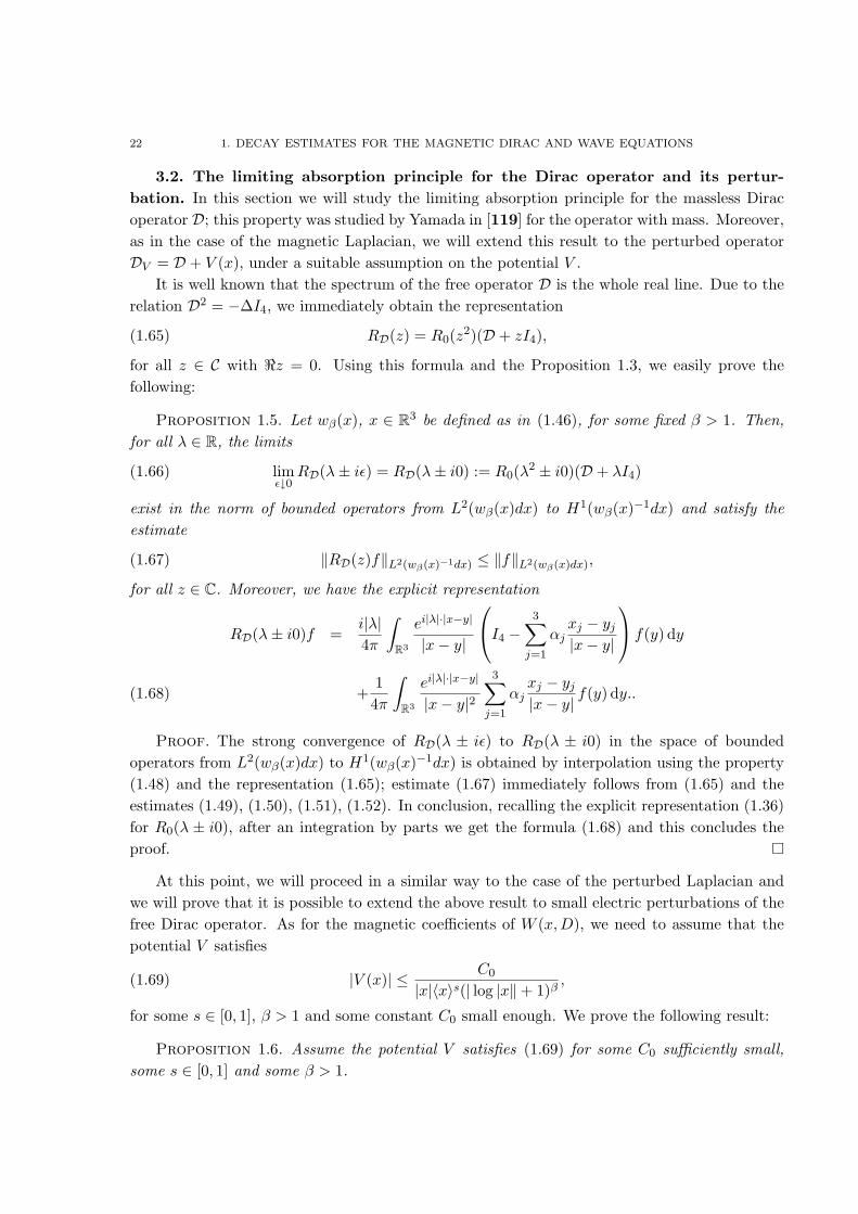
3.2. The limiting absorption principle for the Dirac operator and its pertur-bation. In this section we will study the limiting absorption principle for the massless Diracoperator D; this property was studied by Yamada in [119] for the operator with mass. Moreover,as in the case of the magnetic Laplacian, we will extend this result to the perturbed operatorDV = D + V (x), under a suitable assumption on the potential V .
It is well known that the spectrum of the free operator D is the whole real line. Due to therelation D2 = −∆I4, we immediately obtain the representation
(1.65) RD(z) = R0(z2)(D + zI4),
for all z ∈ C with <z = 0. Using this formula and the Proposition 1.3, we easily prove thefollowing:
Proposition 1.5. Let wβ(x), x ∈ R3 be defined as in (1.46), for some fixed β > 1. Then,for all λ ∈ R, the limits
(1.66) limε↓0
RD(λ± iε) = RD(λ± i0) := R0(λ2 ± i0)(D + λI4)
exist in the norm of bounded operators from L2(wβ(x)dx) to H1(wβ(x)−1dx) and satisfy theestimate
(1.67) ‖RD(z)f‖L2(wβ(x)−1dx) ≤ ‖f‖L2(wβ(x)dx),
for all z ∈ C. Moreover, we have the explicit representation
RD(λ± i0)f =i|λ|4π
∫R3
ei|λ|·|x−y|
|x− y|
I4 − 3∑j=1
αjxj − yj
|x− y|
f(y) dy
+14π
∫R3
ei|λ|·|x−y|
|x− y|23∑
j=1
αjxj − yj
|x− y|f(y) dy..(1.68)
Proof. The strong convergence of RD(λ ± iε) to RD(λ ± i0) in the space of boundedoperators from L2(wβ(x)dx) to H1(wβ(x)−1dx) is obtained by interpolation using the property(1.48) and the representation (1.65); estimate (1.67) immediately follows from (1.65) and theestimates (1.49), (1.50), (1.51), (1.52). In conclusion, recalling the explicit representation (1.36)for R0(λ ± i0), after an integration by parts we get the formula (1.68) and this concludes theproof. �
At this point, we will proceed in a similar way to the case of the perturbed Laplacian andwe will prove that it is possible to extend the above result to small electric perturbations of thefree Dirac operator. As for the magnetic coefficients of W (x,D), we need to assume that thepotential V satisfies
(1.69) |V (x)| ≤ C0
|x|〈x〉s(| log |x‖+ 1)β,
for some s ∈ [0, 1], β > 1 and some constant C0 small enough. We prove the following result:
Proposition 1.6. Assume the potential V satisfies (1.69) for some C0 sufficiently small,some s ∈ [0, 1] and some β > 1.

3. THE LIMITING ABSORPTION PRINCIPLE 23
Then the operator I + V RD is invertible on the weighted space L2(wβ(x)〈x〉2sdx), and theinverse operators (I + V RD(z))−1 are uniformly bounded for all z ∈ C. Moreover, the stronglimiting absorption principle holds for R(z), in the following sense:
(i) the limits
(1.70) limε↓0
R(λ± iε) = R(λ± i0)
exist in the norm of bounded operators from L2(wβ(x)dx) to H1(w−1β (x)dx);
(ii) the following estimate
(1.71) ‖R(z)f‖L2(wβ(x)−1dx) ≤ C(β) · ‖f‖L2(wβ(x)dx)
holds for all z ∈ C, z 6= 0.
Proof. The argument is the same of the proof of Proposition 1.4 for the magnetic part ofW . First we observe that, by hypothesis (1.69), we have
‖w1/2β 〈x〉sV (x)RDf‖L2 ≤ ‖wβ〈x〉sV (x)‖L∞‖w−1/2
β RDf‖L2 ≤ C0 · ‖w−1/2β f‖L2 .
Hence we obtain the estimate
‖w1/2β 〈x〉sV (x)RD(z)f‖L2 ≤ ‖w1/2
β 〈x〉sf‖L2 ,
uniformly in z ∈ C; thus we can invert the operator I +V RD by a Neumann series on the spaceL2(wβdx). Again, we can exploit the representation
(1.72) R(z) = RD(z)(I + V RD(z))−1.
By property (1.66) of Proposition 1.5 and the uniform bounds of (I + V RD)−1, it follows thatthe limits in (1.70) exist in a weak sense. Then we can procede as in the previous cases, usingLemma 1.1 and obtain (i). In conclusion, the estimate (ii) is an immediate consequence of (1.72)and the inequality (1.67). This concludes the proof. �
In the following we shall also need a weaker version of the last result: we shall require thatV satisfies
(1.73) |V (x)| ≤ C0
|x|1/2〈x〉s(| log |x‖+ 1)β/2,
for some s > 12 , β > 1 and some constant C0 small enough. Then we have
Corollary 1.1. Assume the potential V satisfies (1.53) for some C0 sufficiently small,s > 1
2 and β > 1.Then the operators I+V RD are invertible on the space L2(〈x〉2sdx), and the inverse operators
(I + V RD(z))−1 are uniformly bounded for all z ∈ C. Moreover, the strong limiting absorptionprinciple holds for R(z), in the following sense:
(i) the limits
(1.74) limε↓0
R(λ± iε) = R(λ± i0)
exist in the norm of bounded operators from L2(〈x〉2sdx) to H1(〈x〉−2sdx);
24 1. DECAY ESTIMATES FOR THE MAGNETIC DIRAC AND WAVE EQUATIONS
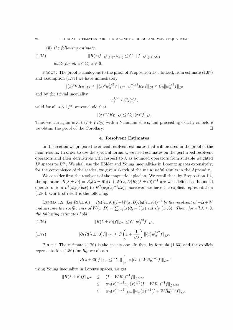
(ii) the following estimate
(1.75) ‖R(z)f‖L2(〈x〉−2sdx) ≤ C · ‖f‖L2(〈x〉2sdx)
holds for all z ∈ C, z 6= 0.
Proof. The proof is analogous to the proof of Proposition 1.6. Indeed, from estimate (1.67)and assumption (1.73) we have immediately
‖〈x〉sV RD‖L2 ≤ ‖〈x〉sw1/2β V ‖L∞‖w−1/2
β RDf‖L2 ≤ C0‖w1/2β f‖L2
and by the trivial inequalityw
1/2β ≤ Cs〈x〉s,
valid for all s > 1/2, we conclude that
‖〈x〉sV RD‖L2 ≤ C0‖〈x〉sf‖L2 .
Thus we can again invert (I + V RD) with a Neumann series, and proceeding exactly as beforewe obtain the proof of the Corollary. �
4. Resolvent Estimates
In this section we prepare the crucial resolvent estimates that will be used in the proof of themain results. In order to use the spectral formula, we need estimates on the perturbed resolventoperators and their derivatives with respect to λ as bounded operators from suitable weightedLp spaces to L∞. We shall use the Holder and Young inequalities in Lorentz spaces extensively;for the convenience of the reader, we give a sketch of the main useful results in the Appendix.
We consider first the resolvent of the magnetic laplacian. We recall that, by Proposition 1.4,the operators R(λ ± i0) = R0(λ ± i0)(I + W (x,D)R0(λ ± i0))−1 are well defined as boundedoperators from L2(wβ(x)dx) to H2(wβ(x)−1dx); moreover, we have the explicit representation(1.36). Our first result is the following:
Lemma 1.2. Let R(λ±i0) = R0(λ±i0)(I+W (x,D)R0(λ±i0))−1 be the resolvent of −∆+Wand assume the coefficients of W (x,D) =
∑aj(x)∂j + b(x) satisfy (1.53). Then, for all λ ≥ 0,
the following estimates hold:
(1.76) ‖R(λ± i0)f‖L∞ ≤ C‖w1/2β f‖L2 ,
(1.77) ‖∂λR(λ± i0)f‖L∞ ≤ C
(1 +
1√λ
)‖〈x〉w1/2
β f‖L2 .
Proof. The estimate (1.76) is the easiest one. In fact, by formula (1.63) and the explicitrepresentation (1.36) for R0, we obtain
‖R(λ± i0)f‖L∞ ≤ C · ‖ 1|x|
∗ |(I +WR0)−1f |‖L∞ ;
using Young inequality in Lorentz spaces, we get
‖R(λ± i0)f‖L∞ ≤ ‖(I +WR0)−1f‖L3/2,1
≤ ‖wβ(x)−1/2wβ(x)1/2(I +WR0)−1f‖L3/2,1
≤ ‖wβ(x)−1/2‖L6,2‖wβ(x)1/2(I +WR0)−1f‖L2 .

4. RESOLVENT ESTIMATES 25
The uniform bound for the operators (I+WR0)−1 proved in Proposition 1.4 and the observationthat w−1/2
β ∈ L6,2, for all β > 1 (see Proposition 1.8) are sufficient now to conclude the proof ofestimate (1.76).
In order to proceed with the proof of (1.77) we observe that from (1.36) we immediatelyobtain the following explicit representations, for all λ > 0:
(1.78) ∂λR0(λ± i0)f = R20(λ± i0)f = ± i
8π√λ
∫ ∞
0e±i
√λ|x−y|f(y)dy,
(1.79) ∂jR20(λ± i0)f = ± 1
8π
∫ ∞
0e±i
√λ|x−y|
∑ xj − yj
|x− y|f(y)dy.
At this point, differentiating in (1.63) we get
(1.80) ∂λR(λ± i0) = A+B
where
A = R20(λ± i0)(I +WR0(λ± i0))−1
and
B = R0(λ± i0)(I +WR0(λ± i0))−1WR20(λ± i0)(I +WR0(λ± i0))−1.
We treat separately the two terms. By (1.78), we estimate
‖Af‖L∞ ≤ C√λ‖(I +WR0)−1f‖L1
≤ C√λ‖〈x〉−1wβ(x)−1/2‖L2‖〈x〉wβ(x)1/2(I +WR0)−1f‖L2 .
We observe (Proposition 1.8) that 〈x〉−1wβ(x)−1/2 ∈ L2 for all β > 1 and, by the uniform boundfor the norms of (I +WR0)−1 in the space of bounded operators onto L2(〈x〉wβ(x)dx) for (seeProposition 1.4), we conclude that, for some C > 0
(1.81) ‖Af‖L∞ ≤ C√λ‖〈x〉wβ(x)1/2f‖L2 .
For the estimate of the term B, we start with some computation on the operator WR20. Using
the representation (1.79), we obtain
‖w1/2β aj∂jR
20f‖L2 ≤ ‖w1/2
β aj‖L2‖∂jR20f‖L∞ ≤ C · ‖w1/2
β aj‖L2‖f‖L1 .
By the above observation that
‖f‖L1 ≤ ‖〈x〉w1/2β (x)f‖L2 ,
it turns out that, if w1/2β aj ∈ L2, then
(1.82) ‖wβ(x)1/2aj(x)∂jR20f‖L2 ≤ C · ‖〈x〉w1/2
β (x)f‖L2 .
In a similar way, using (1.78), we have
‖w1/2β bR2
0f‖L2 ≤ ‖w1/2β b(x)‖L2‖R2
0f‖L∞ ≤ C√λ‖w1/2
β b‖L2‖f‖L1 .
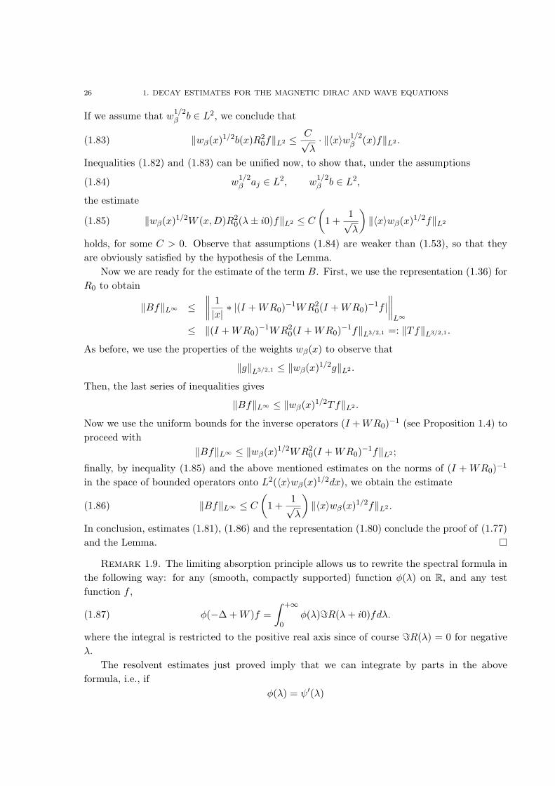
26 1. DECAY ESTIMATES FOR THE MAGNETIC DIRAC AND WAVE EQUATIONS
If we assume that w1/2β b ∈ L2, we conclude that
(1.83) ‖wβ(x)1/2b(x)R20f‖L2 ≤
C√λ· ‖〈x〉w1/2
β (x)f‖L2 .
Inequalities (1.82) and (1.83) can be unified now, to show that, under the assumptions
(1.84) w1/2β aj ∈ L2, w
1/2β b ∈ L2,
the estimate
(1.85) ‖wβ(x)1/2W (x,D)R20(λ± i0)f‖L2 ≤ C
(1 +
1√λ
)‖〈x〉wβ(x)1/2f‖L2
holds, for some C > 0. Observe that assumptions (1.84) are weaker than (1.53), so that theyare obviously satisfied by the hypothesis of the Lemma.
Now we are ready for the estimate of the term B. First, we use the representation (1.36) forR0 to obtain
‖Bf‖L∞ ≤∥∥∥∥ 1|x|
∗ |(I +WR0)−1WR20(I +WR0)−1f |
∥∥∥∥L∞
≤ ‖(I +WR0)−1WR20(I +WR0)−1f‖L3/2,1 =: ‖Tf‖L3/2,1 .
As before, we use the properties of the weights wβ(x) to observe that
‖g‖L3/2,1 ≤ ‖wβ(x)1/2g‖L2 .
Then, the last series of inequalities gives
‖Bf‖L∞ ≤ ‖wβ(x)1/2Tf‖L2 .
Now we use the uniform bounds for the inverse operators (I +WR0)−1 (see Proposition 1.4) toproceed with
‖Bf‖L∞ ≤ ‖wβ(x)1/2WR20(I +WR0)−1f‖L2 ;
finally, by inequality (1.85) and the above mentioned estimates on the norms of (I + WR0)−1
in the space of bounded operators onto L2(〈x〉wβ(x)1/2dx), we obtain the estimate
(1.86) ‖Bf‖L∞ ≤ C
(1 +
1√λ
)‖〈x〉wβ(x)1/2f‖L2 .
In conclusion, estimates (1.81), (1.86) and the representation (1.80) conclude the proof of (1.77)and the Lemma. �
Remark 1.9. The limiting absorption principle allows us to rewrite the spectral formula inthe following way: for any (smooth, compactly supported) function φ(λ) on R, and any testfunction f ,
(1.87) φ(−∆ +W )f =∫ +∞
0φ(λ)=R(λ+ i0)fdλ.
where the integral is restricted to the positive real axis since of course =R(λ) = 0 for negativeλ.
The resolvent estimates just proved imply that we can integrate by parts in the aboveformula, i.e., if
φ(λ) = ψ′(λ)
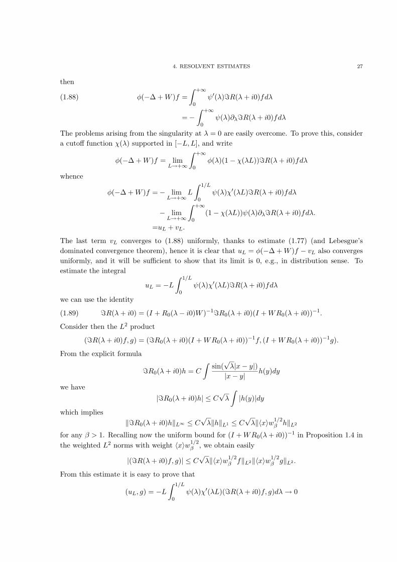
4. RESOLVENT ESTIMATES 27
then
φ(−∆ +W )f =∫ +∞
0ψ′(λ)=R(λ+ i0)fdλ(1.88)
=−∫ +∞
0ψ(λ)∂λ=R(λ+ i0)fdλ
The problems arising from the singularity at λ = 0 are easily overcome. To prove this, considera cutoff function χ(λ) supported in [−L,L], and write
φ(−∆ +W )f = limL→+∞
∫ +∞
0φ(λ)(1− χ(λL))=R(λ+ i0)fdλ
whence
φ(−∆ +W )f =− limL→+∞
L
∫ 1/L
0ψ(λ)χ′(λL)=R(λ+ i0)fdλ
− limL→+∞
∫ +∞
0(1− χ(λL))ψ(λ)∂λ=R(λ+ i0)fdλ.
=uL + vL.
The last term vL converges to (1.88) uniformly, thanks to estimate (1.77) (and Lebesgue’sdominated convergence theorem), hence it is clear that uL = φ(−∆ +W )f − vL also convergesuniformly, and it will be sufficient to show that its limit is 0, e.g., in distribution sense. Toestimate the integral
uL = −L∫ 1/L
0ψ(λ)χ′(λL)=R(λ+ i0)fdλ
we can use the identity
(1.89) =R(λ+ i0) = (I +R0(λ− i0)W )−1=R0(λ+ i0)(I +WR0(λ+ i0))−1.
Consider then the L2 product
(=R(λ+ i0)f, g) = (=R0(λ+ i0)(I +WR0(λ+ i0))−1f, (I +WR0(λ+ i0))−1g).
From the explicit formula
=R0(λ+ i0)h = C
∫sin(
√λ|x− y|)
|x− y|h(y)dy
we have
|=R0(λ+ i0)h| ≤ C√λ
∫|h(y)|dy
which implies‖=R0(λ+ i0)h‖L∞ ≤ C
√λ‖h‖L1 ≤ C
√λ‖〈x〉w1/2
β h‖L2
for any β > 1. Recalling now the uniform bound for (I +WR0(λ+ i0))−1 in Proposition 1.4 inthe weighted L2 norms with weight 〈x〉w1/2
β , we obtain easily
|(=R(λ+ i0)f, g)| ≤ C√λ‖〈x〉w1/2
β f‖L2‖〈x〉w1/2β g‖L2 .
From this estimate it is easy to prove that
(uL, g) = −L∫ 1/L
0ψ(λ)χ′(λL)(=R(λ+ i0)f, g)dλ→ 0

28 1. DECAY ESTIMATES FOR THE MAGNETIC DIRAC AND WAVE EQUATIONS
as L→ +∞, which concludes the argument.
We will prove now an analogue of Lemma 1.2 for the Dirac operator. In what follows,R(z) = (−zI4 +D+V )−1 denotes the resolvent of the perturbed Dirac operator. Our approachhere will be slightly different: we shall use the formula
(1.90) R(z) = RD(z) +RD(z)V (x)RD(z)(I + V (x)RD(z))−1,
valid for all z ∈ C (to be interpreted of course, for z = λ ∈ R, as the extended resolventsR(λ) := R(λ ± i0) on the weighted L2 spaces, as given by Proposition 1.6 and Corollary 1.1).When inserted in the spectral formula, the first term RD at the right hand side reproduces thesolution to the free Dirac equation, and the main part of our proof will be the estimate of secondterm
(1.91) Q := RDV RD(I + V RD)−1.
To this end, we shall need an explicit representation for RD(λ ± i0), which is easily obtainedfrom the formula
(1.92) RD(λ± i0) = R0(λ2 ± i0)(D + λI4).
Recalling (1.36), after an integration by parts we obtain
RD(λ± i0)f =iλ
4π
∫R3
e±iλ|x−y|
|x− y|
I4 ∓ 3∑j=1
αjxj − yj
|x− y|
f(y)dy
+14π
∫R3
e±iλ|x−y|
|x− y|23∑
j=1
αjxj − yj
|x− y|f(y)dy.(1.93)
¿From here we derive immediately an analogous representation for
R2D(λ) =
∂
∂λRD(λ);
indeed, differentiating (1.93) with respect to λ, we get
R2D(λ± i0)f =
λ
4π
∫R3
e±iλ|x−y|
∓I4 +3∑
j=1
αjxj − yj
|x− y|
f(y)dy
± i
4π
∫R3
e±iλ|x−y|
|x− y|
3∑j=1
αjxj − yj
|x− y|f(y)dy.(1.94)
We collect all the necessary estimates in the following lemma (we write for simplicity RD(λ)instead of RD(λ± i0) since the estimates are the same):
Lemma 1.3. Suppose that
(1.95) |V (x)| ≤ C0
|x|1/2〈x〉s(| log |x‖+ 1)β/2,
for some s > 32 , β > 1, C0 > 0. Then the following estimates hold for all ε > 0 small enough
and all λ ∈ R:
(1.96) ‖〈x〉1/2+εV R2D(λ)f‖L2 ≤ Cε · 〈λ〉 · ‖〈x〉3/2+εf‖L2 ,

4. RESOLVENT ESTIMATES 29
(1.97) ‖RD(λ)V RD(λ)f‖L∞ ≤ Cε · 〈λ〉2 · ‖〈x〉1/2+εf‖L2
(1.98) ‖R2D(λ)V RD(λ)f‖L∞ + ‖RD(λ)V R2
D(λ)f‖L∞ ≤ Cε · 〈λ〉2 · ‖〈x〉3/2+εf‖L2
for some C = Cε independent of λ.
Proof. In the following we shall use the shorthand notation, for s ∈ R,
(1.99) ‖f‖L2γ
:= ‖〈x〉γf‖L2
From the explicit representations (1.93) and (1.94) we have the simple pointwise estimates
(1.100) |RD(λ)f | ≤ C(|λ| · |x|−1 + |x|−2) ∗ f, |R2D(λ)f | ≤ C(|λ|+ |x|−1) ∗ f.
Since |x|−1 ∈ L3,∞, by the Young inequality in Lorentz spaces (see the Appendix) we get
‖V R2D(λ)f‖L2
γ≤ ‖V ‖L2
γ· |λ| · ‖1 ∗ f‖L∞ + ‖V ‖L2
γ‖|x|−1 ∗ f‖L∞
≤ ‖V ‖L2γ(|λ| · ‖f‖L1 + ‖f‖L3/2,1) .
By the obvious inequalities valid for all ε > 0
(1.101) ‖f‖L1 ≤ C(ε)‖f‖L23/2+ε
, ‖f‖L3/2,1 ≤ C(ε)‖f‖L21/2+ε
,
we arrive at the first estimate
(1.102) ‖V R2D(λ)f‖L2
γ≤ C(ε)‖V ‖L2
γ〈λ〉‖f‖L2
3/2+ε.
Since ‖V ‖L2γ<∞ by assumption (1.95) as soon as γ = 1/2+ε < s−1, we see that (1.96) follows
provided ε is suitably small.In a similar way, in order to prove (1.97) we use again (1.100) and we write (recall that
|x|−2 ∈ L3/2,∞)
‖RD(λ)V RD(λ)f‖L∞ ≤ C(|λ| · ‖|x|−1 ∗ V RDf‖L∞ + ‖|x|−2 ∗ V RDf‖L∞
)≤ C (|λ| · ‖V RD(λ)f‖L3/2,1 + ‖V RD(λ)f‖L3,1) .
For the first term we can write, recalling again (1.100),
‖V RD(λ)f‖L3/2,1 ≤ ‖V ‖L3/2,1 |λ| · ‖|x|−1 ∗ f‖L∞ + ‖V ‖L2‖|x|−2 ∗ f‖L6,2(1.103)
≤ ‖V ‖L3/2,1 |λ| · ‖f‖L3/2,1 + ‖V ‖L2‖f‖L2
≤ (‖V ‖L3/2,1 |λ|+ ‖V ‖L2) ‖f‖L23/2+ε
(see (1.101)), while for the second term we have
‖V RD(λ)f‖L3,1 ≤ ‖V ‖L3,1 |λ| · ‖|x|−1 ∗ f‖L∞ + ‖V ‖L6,2‖|x|−2 ∗ f‖L6,2(1.104)
≤ ‖V ‖L3,1 |λ| · ‖f‖L3/2,1 + ‖V ‖L6,2‖f‖L2
≤ (‖V ‖L3,1 |λ|+ ‖V ‖L6,2) ‖f‖L23/2+ε
where we have used (1.101) and the trivial inequality ‖f‖L2 ≤ ‖f‖L2γ, ∀γ > 0. Summing up, we
get
(1.105) ‖RD(λ)V RD(λ)f‖L∞ ≤ C · C(V )〈λ〉2‖f‖L23/2+ε
where the quantity
(1.106) C(V ) := ‖V ‖L3/2,1 + ‖V ‖L3,1 + ‖V ‖L6,2 + ‖V ‖L2 <∞
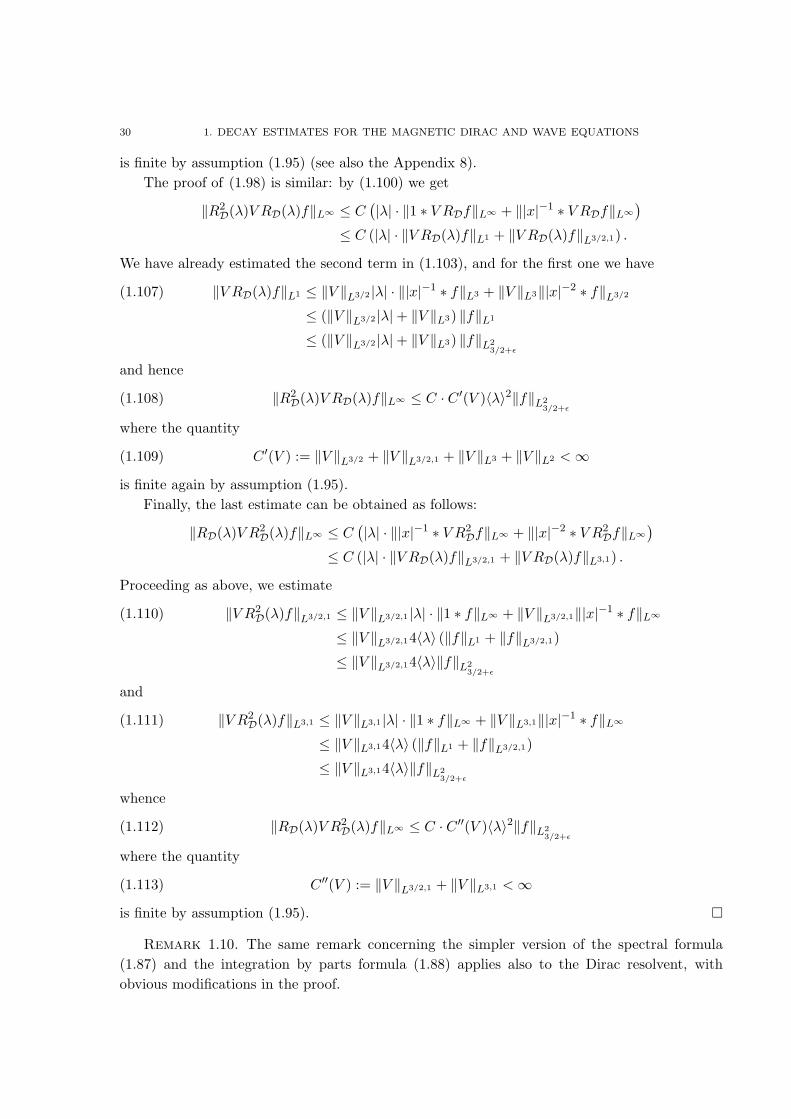
30 1. DECAY ESTIMATES FOR THE MAGNETIC DIRAC AND WAVE EQUATIONS
is finite by assumption (1.95) (see also the Appendix 8).The proof of (1.98) is similar: by (1.100) we get
‖R2D(λ)V RD(λ)f‖L∞ ≤ C
(|λ| · ‖1 ∗ V RDf‖L∞ + ‖|x|−1 ∗ V RDf‖L∞
)≤ C (|λ| · ‖V RD(λ)f‖L1 + ‖V RD(λ)f‖L3/2,1) .
We have already estimated the second term in (1.103), and for the first one we have
‖V RD(λ)f‖L1 ≤ ‖V ‖L3/2 |λ| · ‖|x|−1 ∗ f‖L3 + ‖V ‖L3‖|x|−2 ∗ f‖L3/2(1.107)
≤ (‖V ‖L3/2 |λ|+ ‖V ‖L3) ‖f‖L1
≤ (‖V ‖L3/2 |λ|+ ‖V ‖L3) ‖f‖L23/2+ε
and hence
(1.108) ‖R2D(λ)V RD(λ)f‖L∞ ≤ C · C ′(V )〈λ〉2‖f‖L2
3/2+ε
where the quantity
(1.109) C ′(V ) := ‖V ‖L3/2 + ‖V ‖L3/2,1 + ‖V ‖L3 + ‖V ‖L2 <∞
is finite again by assumption (1.95).Finally, the last estimate can be obtained as follows:
‖RD(λ)V R2D(λ)f‖L∞ ≤ C
(|λ| · ‖|x|−1 ∗ V R2
Df‖L∞ + ‖|x|−2 ∗ V R2Df‖L∞
)≤ C (|λ| · ‖V RD(λ)f‖L3/2,1 + ‖V RD(λ)f‖L3,1) .
Proceeding as above, we estimate
‖V R2D(λ)f‖L3/2,1 ≤ ‖V ‖L3/2,1 |λ| · ‖1 ∗ f‖L∞ + ‖V ‖L3/2,1‖|x|−1 ∗ f‖L∞(1.110)
≤ ‖V ‖L3/2,14〈λ〉 (‖f‖L1 + ‖f‖L3/2,1)
≤ ‖V ‖L3/2,14〈λ〉‖f‖L23/2+ε
and
‖V R2D(λ)f‖L3,1 ≤ ‖V ‖L3,1 |λ| · ‖1 ∗ f‖L∞ + ‖V ‖L3,1‖|x|−1 ∗ f‖L∞(1.111)
≤ ‖V ‖L3,14〈λ〉 (‖f‖L1 + ‖f‖L3/2,1)
≤ ‖V ‖L3,14〈λ〉‖f‖L23/2+ε
whence
(1.112) ‖RD(λ)V R2D(λ)f‖L∞ ≤ C · C ′′(V )〈λ〉2‖f‖L2
3/2+ε
where the quantity
(1.113) C ′′(V ) := ‖V ‖L3/2,1 + ‖V ‖L3,1 <∞
is finite by assumption (1.95). �
Remark 1.10. The same remark concerning the simpler version of the spectral formula(1.87) and the integration by parts formula (1.88) applies also to the Dirac resolvent, withobvious modifications in the proof.

5. PROOF OF THEOREM 1.1 31
5. Proof of Theorem 1.1
Let (ϕj)j=0,1,... be a standard Paley-Littlewood partition of the unity, with the properties
(1.114) ϕj(λ) = ϕ0(2−jλ), ϕ0 +∑j≥1
ϕj = 1,
for a suitable ϕ0 ∈ C∞0 . We consider the Cauchy problem
(1.115){utt(t, x)−∆u(t, x) +W (x,D)u = 0u(0, x) = 0, ut(0, x) = ϕj(
√−∆ +W )g(x),
The solution can be represented using the spectral formula as follows:
(1.116) u(t, x) =1
2πi
∫ +∞
0ϕj(
√λ)
sin(t√λ)√
λR(λ)gdλ,
and after an integration by parts (see Remark 1.9) this gives
(1.117) u(t, x) =C
t
∫ +∞
0cos(t
√λ)[∂λϕj(
√λ)R(λ)g + ϕj(
√λ)∂λR(λ)g
]dλ.
Thus, recalling estimates (1.76) and (1.77), we have
|u(t, x)| ≤ C
t‖〈x〉w1/2
β g‖L2
∫ +∞
0
(|∂λϕj(
√λ)|+
(1 +
1√λ
)|ϕj(
√λ)|)dλ
and a change of variables λ = 22jµ in the integral gives immediately
(1.118) |u(t, x)| ≤ C
t22j‖〈x〉w1/2
β g‖L2
with some constant C independent of j and g.If we now define as usual
ϕj = ϕj−1 + ϕj + ϕj+1, ϕ−1 = 0,
so that ϕj ≡ ϕjϕj , we see that the Cauchy problem (1.115) can be written equivalently
(1.119){utt(t, x)−∆u(t, x) +W (x,D)u = 0u(0, x) = 0, ut(0, x) = ϕj(
√−∆W )ϕj(
√−∆W )g(x),
hence our estimate (1.118) implies also the estimate
(1.120) |u(t, x)| ≤ C
t22j‖〈x〉w1/2
β ϕj(√−∆W )g‖L2 .
Finally, consider the original Cauchy problem (1.6), and decompose g as a sum
g =∑j≥0
ϕj(√−∆W )g(x).
By estimate (1.120) we obtain easily estimate (1.9).
(1.121) |u(t, x)| ≤ C
t
∑j≥0
22j‖〈x〉w1/2β ϕj(
√−∆W )g‖L2 .
The computations in the case of initial data of the form
u(0, x) = f, ut(0, x) = 0
are completely analogous, and we thus obtain estimate (1.12).
32 1. DECAY ESTIMATES FOR THE MAGNETIC DIRAC AND WAVE EQUATIONS
Remark 1.11. In view of the application to the Dirac system, the following remark will beuseful. If the initial datum g has the form
(1.122) g = (−∆W )sh
for some s > 0, a direct application of estimate (1.121) would give only
(1.123) |u(t, x)| ≤ C
t
∑j≥0
22j‖〈x〉w1/2β ϕj(
√−∆W )(−∆W )sh‖L2 .
Actually, if we go back to the spectral formula (1.117), we see that the solution can be written
(1.124) u(t, x) =C
t
∫ +∞
0λs/2 cos(t
√λ)[∂λϕj(
√λ)R(λ)h+ ϕj(
√λ)∂λR(λ)h
]dλ.
with an additional factor λs/2. Thus, proceeding as above, we arrive at the simpler estimate
(1.125) |u(t, x)| ≤ C
t
∑j≥0
2(2+s)j‖〈x〉w1/2β ϕj(
√−∆W )h‖L2 .
We now prove estimate (1.11) under the stronger assumption (1.10) on the potentialW (x,D).Consider first the case of initial data of the form
u(0, x) = 0, ut(0, x) = g.
We can write g as follows:
g = (1−∆ +W )−1−ε(1−∆ +W )1+εg
for some fixed ε > 0. Then the solution u can be represented as
u(t, x) =1
2πi
∫ +∞
0ψ(√λ)
sin(t√λ)√
λR(λ)hdλ
whereh = (1−∆ +W )1+εg, ψ(
√λ) = (1 + λ)1+ε.
Proceeding as above, after an integration by parts we arrive at
|u(t, x)| ≤ C
t‖〈x〉w1/2
β h‖L2
∫ +∞
0((1 + λ)−1−ε + (1 + λ)−2−ε)dλ
and hence
(1.126) |u(t, x)| ≤ C
t‖〈x〉w1/2
β (1−∆ +W )1+εg‖L2 ≤C
t‖〈x〉3/2+ε(1−∆ +W )1+εg‖L2 .
To conclude the proof of the Theorem, it remains to show that
(1.127) ‖〈x〉3/2+ε(1−∆ +W )1+εg‖L2 ≤ ‖〈x〉3/2+εg‖H2+2ε .
We start from the inequality
‖〈x〉s(1−∆ +W )f‖L2 ≤ ‖〈x〉sf‖H2
which is obviously valid for any s ≥ 0. By a standard complex interpolation argument, interpo-lating with the trivial inequality
‖〈x〉sf‖L2 ≤ ‖〈x〉sf‖L2
we obtain that‖〈x〉s(1−∆ +W )εf‖L2 ≤ ‖〈x〉sf‖H2ε
6. PROOF OF THEOREM 1.2 33
for all 0 ≤ ε ≤ 1 and all s ≥ 0. This implies
(1.128) ‖〈x〉s(1−∆ +W )1+εf‖L2 ≤ ‖〈x〉s(1−∆ +W )f‖H2ε ≤ ‖〈x〉sf‖H2+2ε + ‖〈x〉sWf‖H2ε .
The last term is of the form
(1.129) ‖〈x〉sW (x,D)f‖H2ε ≤ ‖〈x〉sa(x)Df‖H2ε + ‖〈x〉sb(x)f‖H2ε ;
in order to estimate it, we recall the Kato-Ponce inequality (see [64])
(1.130) ‖〈D〉q(vw)‖Lp ≤ C‖〈D〉qv‖Lp1‖w‖Lp2 + C‖v‖Lp3‖〈D〉qw‖Lp4
which is valid for all q ≥ 0, p−1 = p11 + p−1
2 = p−13 + p−1
4 . With the choices v(x) = a(x),w(x) = 〈x〉sDf(x), q = 2ε, p1 = p3 = ∞ and p2 = p4 = 2, we obtain
‖〈D〉2ε〈x〉sa(x)Df‖L2 ≤ C‖〈D〉2εa‖L∞‖〈x〉sDf‖L2 + C‖a‖L∞‖〈D〉2ε(〈x〉sDf)‖L2 .
Now it is clear that
‖〈D〉2ε(〈x〉sDf)‖L2 ≤ C‖〈x〉sf‖H1+2ε
(use again complex interpolation between the cases ε = 0 and ε = 1) and in conclusion we obtain
‖〈D〉2ε〈x〉sa(x)Df‖L2 ≤ C‖〈D〉2εa‖L∞‖〈x〉sf‖H1+2ε .
Here we have used the simple fact that
‖a‖L∞ ≤ C‖〈D〉2εa‖L∞ .
The corresponding estimate for the electric term is analogous (actually simpler):
‖〈D〉2ε〈x〉sb(x)f‖L2 ≤ C‖〈D〉2εb‖L∞‖〈x〉sf‖H2ε .
Recalling now (1.128) and (1.129) we conclude the proof of estimate (1.11).On the other hand, when the data are of the form
u(0, x) = f, ut(0, x) = 0
the computations are completely analogous and we obtain estimate (1.14) under the strongerassumptions (1.13) on the coefficients.
6. Proof of Theorem 1.2
Remark 1.12. We notice that Theorem 1.1 (and Remark 1.4) can be trivially extended toa system of wave equations of the form
(1.131) utt − (∇+ iA(x))2u+B(x)u = 0
where u(t, x) is a CN valued function and A1(x), A2(x), A3(x), B(x) are CN×N matrices whosecoefficients satisfy the assumptions of the Theorem. The resulting dispersive estimates haveexactly the same form as in the scalar case.
Consider now the Cauchy problem
(1.132){iut −Du− V (x)u = 0u(0, x) = f(x).

34 1. DECAY ESTIMATES FOR THE MAGNETIC DIRAC AND WAVE EQUATIONS
If we apply to the pertubed Dirac system the operator i∂t + D + V we obtain that u is also asolution of a 4×4 system of perturbed wave equations of the form (1.131) with
(1.133) Aj(x) = −12(αjV (x) + V (x)αj),
(1.134) B(x) = DV (x) + V (x)2 +A21 +A2
2 +A23 + i
∑∂jAj
and initial data
(1.135) u(0, x) = f, ut(0, x) = i−1(D + V )f.
Note that the perturbed operator
(1.136) −∆W = −(∇+ iA(x))2 +B(x)
is exactly the square of the operator D + V :
(1.137) −∆W = (D + V )2
and hence the initial data for (1.131) can be written
(1.138) u(0, x) = f, ut(0, x) = i−1(−∆W )1/2f.
We are in position to apply to the solution u the estimates already proved in Theorem 1.1;keeping Remark 1.11 into account, we arrive easily at the estimate
(1.139) |u(t, x)| ≤ C
t
∑j≥0
23j‖〈x〉w1/2β ϕj(D + V )f‖L2 ,
provided the coefficients aj(x) and b(x) satisfy the assumptions (1.8). Recalling the explicitform (1.133) of the coefficients in terms of V (x), we see that V must satisfy the conditions
|V (x)| ≤ C0
|x|〈x〉(| log |x||+ 1)β
from the magnetic term, and
|V (x)2|+ |DV (x)| ≤ C0
|x|2(| log |x||+ 1)β,
from the electric term, for some β > 1 and some small constant C0. Summing up, we obtainthat (1.139) holds under assumption (1.17).
The estimate in terms of the Sobolev norm can be obtained in exactly the same way as forthe perturbed wave equation. Indeed, proceeding as in (1.126) we arrive at the estimate
(1.140) |u(t, x)| ≤ C
t‖〈x〉3/2+ε(−∆W )3/2+εf‖L2 .
The same arguments used at the end of Section 5 give here
(1.141) |u(t, x)| ≤ C
t‖〈x〉3/2+εf‖H3+2ε
provided〈D〉1+2εAj ∈ L∞, 〈D〉1+2εB ∈ L∞,
which is implied by〈D〉2+2εV ∈ L∞.

7. PROOF OF THEOREM 1.3 35
7. Proof of Theorem 1.3
By exploiting the connection between the massless Dirac and the wave equation, it is easyto obtain an optimal dispersive estimate in the unperturbed case. In order to state it, we recallthe definition of the homogeneous Besov space Bs
1,1. The Besov norm is given by
‖v‖Bs1,1
=∑j∈Z
2js‖φj(√−∆)v‖L1 ,
where φj is a homogeneous Paley-Littlewood sequence, i.e., fixed a test function ψ(r) ∈ C∞0such that ψ(r) = 1 for r < 1, ψ(r) = 0 for r > 2, we have φj(r) = ψ(2−j+2r)−ψ(2−j+1r) for allj ∈ Z.
Now, let u(t, x) be a smooth solution of the free massless Dirac equation
(1.142) iut(t, x) = Du(t, x)
with initial data
(1.143) u(0, x) = f(x).
Then we have:
Proposition 1.7. The solution u(t, x) of problem (1.142),(1.143) satisfies the dispersiveestimate
(1.144) |u(t, x)| ≤ C
t‖f‖B2
1,1.
Proof. Recall the identity
(i∂t +D)(i∂t −D) = (∆− ∂2tt)I4;
if we apply the operator i∂t +D to the system (1.142) we see that u solves the Cauchy problemfor the wave equation
utt −∆u = 0
with initial datau(0, x) = f, ut(0, x) = i−1Df.
Then, as a consequence of the well known decay estimates for solutions to the free wave equation(see e.g. [95]), we obtain
|u(t, x)| ≤ C
t
(‖f‖B2
1,1+ ‖Df‖B1
1,1
)whence (1.144) follows immediately. �
The proof of Theorem 1.3 follows the same lines as the proof of Theorem 1.1. Consider theCauchy problem with frequency truncated data
(1.145){iut(t, x) = DV u(t, x)u(0, x) = ϕj(DV )f,
where (ϕj(λ))j=0,1,... is the standard Paley-Littlewood partition of the unity defined in (1.114).By means of spectral formula, we can represent the solution of (1.145) as
(1.146) u(t, x) =1
2πi
∫ +∞
−∞ϕj(λ)eiλtI[RV (λ)]f dλ.
36 1. DECAY ESTIMATES FOR THE MAGNETIC DIRAC AND WAVE EQUATIONS
Using the identity
(1.147) RV (λ) = RD −RDV RD(I + V RD)−1,
which is valid thanks to Corollary 1.1, we can split the integrals in (1.146) into two terms, thefirst one containing the contribution of the free resolvent RD and the second one containing thecontribution of the operator RDV RD(I + V RD)−1. The first term
A :=1
2πi
∫ +∞
−∞ϕj(λ)eiλt= [RD(λ)] f dλ
was estimated above (see (1.144)); it remains to estimate the term
(1.148) B = − 12πi
∫ +∞
−∞ϕj(λ)eiλt= [Q(λ)] f dλ,
where
Q(λ) := RD(λ)V RD(λ)(I + V RD(λ))−1.
After an integration by parts, we obtain
(1.149) B = − 12πt
[∫ +∞
−∞ϕj(λ)eiλt ∂
∂λI(Q(λ))f dλ+
∫ +∞
−∞ϕ′j(λ)eiλtI[Q(λ)]f dλ
];
an explicit computation shows that
∂Q
∂λ= R2
DV RD(I4 + V RD)−1 +RDV R2D(I4 + V RD)−1
+RDV RD(I4 + V RD)−1V R2D(I4 + V RD)−1.
Now we can apply Lemma 1.3: under assumption (1.21), estimates (1.96), (1.97) and (1.98) aresatisfied, and the Lemma gives
(1.150) ‖Q(λ)f‖L∞ ≤ C〈λ〉2‖〈x〉3/2+εf‖L2 ,
(1.151)∣∣∣∣∣∣∣∣ ∂∂λQ(λ)f
∣∣∣∣∣∣∣∣L∞
≤ C〈λ〉3‖〈x〉3/2+εf‖L2 ,
for some C > 0. Using (1.150) and (1.151) in (1.149) we arrive at the estimate
|B| ≤ C
t‖f‖L2
3/2+ε
[∫ +∞
−∞
(〈λ〉3|ϕj(λ)|+ 〈λ〉2
∣∣ϕ′j(λ)∣∣) dλ
].
Recalling that φj(λ) = φ0(2−jλ), after a change of variables 2−jλ = µ we easily obtain
(1.152) |B| ≤ C
t24j‖〈x〉3/2+εf‖L2 .
From this point on, we can proceed as in the proof of Theorem 1.1 and complete the proof ofTheorem 1.3.

8. AN APPENDIX ON LORENTZ SPACES 37
8. An appendix on Lorentz spaces
For the convenience of the reader, we recall here the definitions and the main properties ofthe Lorentz spaces Lp,q, in view of the applications needed in the proof of our results.
For any measurable function f : Rn → C and any s ≥ 0 we define the upper-level Efs as the
setEf
s := {x : |f(x)| > s}.The non-increasing rearrangement of f is then the function
f∗(t) := inf{s > 0 : |Efs | ≤ t}, t ∈ (0,+∞).
It is also useful to consider the average of f∗ defined by
f∗∗(t) =1t
∫ t
0f∗(r) dr.
The standard definition of the Lorentz spaces is the following:
Definition 1.1. For any 1 ≤ p < ∞ and 1 ≤ q ≤ ∞ we define the quasinorm ‖f‖Lp,q asfollows:
(1.153) ‖f‖Lp,q =
{[∫∞0 (t1/pf∗(t))q dt
t
]1/q, 1 ≤ q <∞
supt>0 t1/pf∗(t), q = ∞.
When p 6= 1, if we replace f∗ with f∗∗ in the above definitions we obtain an equivalent quasinormwhich is actually a norm (see [10], [19]). The Lorentz space Lp,q is defined by
(1.154) Lp,q = {f : ‖f‖Lp,q <∞}.
Moreover we defineL1,1 := L1, L∞,∞ = L∞.
The spaces L∞,q for 1 ≤ q < ∞ are usually left undefined (although L∞,1 is defined in [19] asthe closure of L∞ compactly supported functions in the L∞ norm).
With the above definitions, one obtains the elementary properties
Lp,p = Lp, 1 ≤ p ≤ ∞;
Lp,q1 ⊆ Lp,q2 , 1 < p <∞, 1 ≤ q1 ≤ q2 ≤ ∞(with continuous embedding). When the second index is ∞ we obtain the weak Lebesgue spaces(Marcinkiewicz spaces):
Lp,∞ = Lpw, 1 ≤ p ≤ ∞.
Moreover, the Lorentz spaces can be obtained by an equivalent construction using real interpo-lation:
Lp,q = (Lp0 , Lp1)θ,q, p−1 = (1− θ)p−10 + θp−1
1
providedp0 < p1, p0 < q ≤ ∞, 0 < θ < 1.
An alternative characterization of the Lorentz norm can be given using the so-called atomicdecomposition:

38 1. DECAY ESTIMATES FOR THE MAGNETIC DIRAC AND WAVE EQUATIONS
Lemma 1.4. Let f : Rn → C be a measurable function and let 1 ≤ p < ∞, 1 ≤ q ≤ ∞;then f ∈ Lp,q if and only if there exist a sequnce of sets (Ej)j∈Z and a sequence of numbersa = (aj)j∈Z such that |Ej | = O(2j), a ∈ lq and the following estimate
(1.155) |f(x)| ≤ C∑j∈Z
aj2−j/pχEj (x)
holds, for some C > 0.
It is possible to see that the best constant C in (1.155) is equivalent to the Lorentz norm ofthe function f .
The most useful properties of Lorentz spaces are the Holder and Young inequalities, whichextend the classical ones for Lebesgue spaces. These were originally proved by O’Neil in [80].We collect them in the following theorems:
Theorem 1.5 (Holder inequality). Let f ∈ Lp1,q1 , g ∈ Lp2,q2. The following estimates hold:
• if p1, p2, p ∈]1,∞[, q1, q2, q ∈ [1,∞], then
(1.156) ‖fg‖Lp,q ≤ C‖f‖Lp1,q1‖g‖Lp2,q2 , 1 > p−11 + p−1
2 = p−1, q−11 + q−1
2 ≥ q−1;
• if p1, p2 ∈ [1,∞[, q1, q2 ∈ [1,∞], then
(1.157) ‖fg‖L1 ≤ C‖f‖Lp1,q1‖g‖Lp2,q2 , p−11 + p−1
2 = 1, q−11 + q−1
2 ≥ 1.
We remark that the above statement does not cover the trivial inequality
(1.158) ‖fg‖Lp,q ≤ ‖f‖L∞‖g‖Lp,q
which is evidently true whenever Lp,q is defined.
Theorem 1.6 (Young inequality). Let f ∈ Lp1,q1 , g ∈ Lp2,q2. Then the following estimateshold:
• if p1, p2, p ∈]1,∞[, q1, q2, q ∈ [1,∞], then
(1.159) ‖f ∗ g‖Lp,q ≤ C‖f‖Lp1,q1‖g‖Lp2,q2 , p−11 + p−1
2 = 1 + p−1, q−11 + q−1
2 ≥ q−1;
• if p1, p2 ∈]1,∞[, q1, q2 ∈ [1,∞], then
(1.160) ‖f ∗ g‖L∞ ≤ C‖f‖Lp1,q1‖g‖Lp2,q2 , p−11 + p−1
2 = 1, q−11 + q−1
2 ≥ 1.
As before, we remark that the above statement does not cover the inequality
(1.161) ‖f ∗ g‖Lp,q ≤ C‖f‖L1‖g‖Lp,q
which is easily seen to be true in all cases when Lp.q is defined (e.g., by real interpolation).We conclude this section by studying the weight functions wβ(x) = |x|(| log |x||+ 1)β, with
β > 1 which plays a crucial role in our results; in the following proposition we determine preciselyto which Lorentz the powers w−s
β belong.
Proposition 1.8. For any s > 0, q ∈ [1,∞] we have w−sβ ∈ Ln/s,q, provided β > 1/sq.

8. AN APPENDIX ON LORENTZ SPACES 39
Proof. We will use the equivalent Lorentz norm (1.155). For any j ∈ Z consider the ballBj := B2j/n = {x : |x| ≤ 2j/n} and the rings Ej := Bj+1 \Bj ; it is clear that |Ej | = Cn2j , whereCn depends only on the dimension n. Then, for all x ∈ Rn we have the estimate
|w−sβ (x)| =
∑j∈Z
1|x|s(| log |x||+ 1)βs
χEj (x) ≤ C∑j∈Z
(|j| log 2 + 1)−βs2−js/nχEj (x).
The proof is concluded by the remark that the sequence aj = (|j| log 2 + 1)−βs is in lq if andonly if β > 1/sq. �

CHAPTER 2
Strichartz estimates and Kato-smoothing effect
1. Introduction
Following the previous chapter, we continue the investigation on equations with electromag-netic potentials; here we point our attention to the other dispersive-type estimates we presentedin the Introduction, namely Strichartz and Kato-smoothing estimates. In this chapter we presentsome results in this direction, concerning Schrodinger, Wave, Klein-Gordon and Dirac equations.The reference for the results in the present chapter is [32].
Strichartz estimates have become a standard tool in the study of linear and nonlinear evo-lution equations. They are available for a large class of constant coefficient equations, by themethods of [47] and [66]. In a sense, they represent the modern energy estimates, and areespecially effective for problems of low regularity and global existence for nonlinear equations.
Using the notations LpLq = Lp(Rt;Lq(Rnx)), ‖f‖ . ‖g‖ to mean ‖f‖ ≤ C‖g‖, and Hs
q andHs
q to denote the spaces with norms
‖f‖Hsq
= ‖〈D〉sf‖Lq , ‖f‖Hsq
= ‖|D|sf‖Lq .
where 〈D〉 = (1 −∆)1/2, |D| = (−∆)1/2, the Strichartz estimates for the Schrodinger equationtake the following form: for n ≥ 2,
‖eit∆f‖LpLq . ‖f‖L2 ,
provided the couple (p, q) is Schrodinger admissible:
(2.1)2p
+n
q=n
2, 2 ≤ p ≤ ∞,
2nn− 2
≥ q ≥ 2, q 6= ∞.
The couple (p, q) = (2, 2n/n− 2) is called the endpoint and is allowed when n > 2.For the wave equation the estimates can be written as follows: for n ≥ 3,
‖eit|D|f‖LpH
1q−
1p−
12
q
. ‖f‖L2 ,
provided the couple (p, q) is wave admissible:
(2.2)2p
+n− 1q
=n− 1
2, 2 ≤ p ≤ ∞,
2(n− 1)n− 3
≥ q ≥ 2, q 6= ∞.
The wave equation endpoint is (p, q) = (2, 2(n− 1)/(n− 3)) and is allowed in dimension n > 3.Finally for the Klein-Gordon equation we have: for n ≥ 2,
‖eit〈D〉f‖LpH
1q−
1p−
12
q
. ‖f‖L2 ,
provided (p, q) is Schrodinger admissible (see Section 4 for a proof of the last estimate, for whicha reference is not immediately available).
41
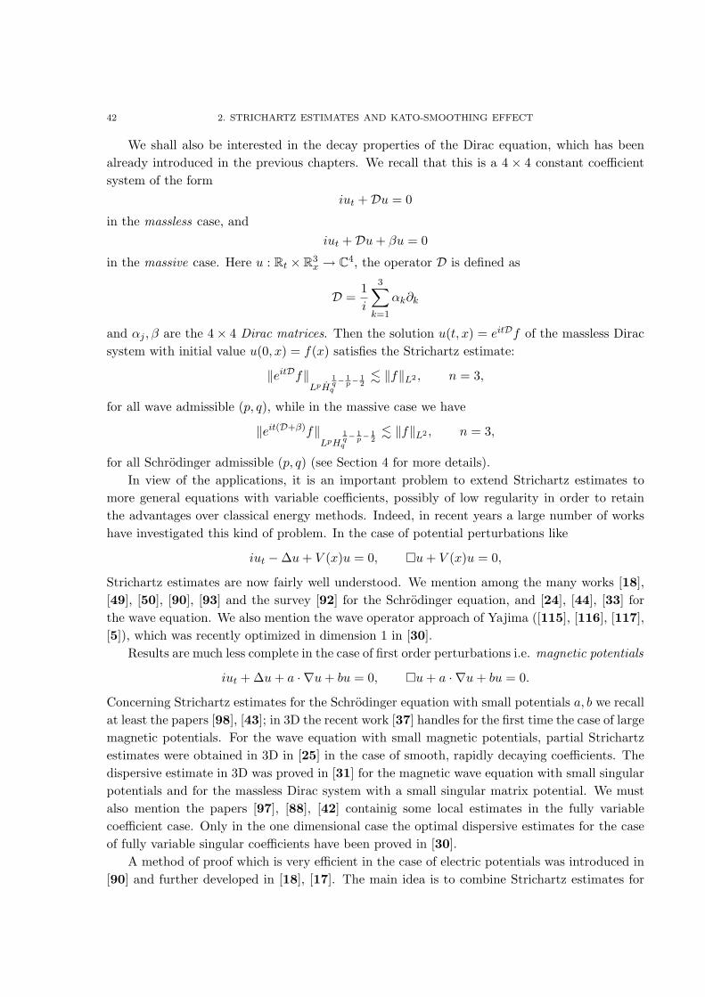
42 2. STRICHARTZ ESTIMATES AND KATO-SMOOTHING EFFECT
We shall also be interested in the decay properties of the Dirac equation, which has beenalready introduced in the previous chapters. We recall that this is a 4 × 4 constant coefficientsystem of the form
iut +Du = 0
in the massless case, andiut +Du+ βu = 0
in the massive case. Here u : Rt × R3x → C4, the operator D is defined as
D =1i
3∑k=1
αk∂k
and αj , β are the 4× 4 Dirac matrices. Then the solution u(t, x) = eitDf of the massless Diracsystem with initial value u(0, x) = f(x) satisfies the Strichartz estimate:
‖eitDf‖LpH
1q−
1p−
12
q
. ‖f‖L2 , n = 3,
for all wave admissible (p, q), while in the massive case we have
‖eit(D+β)f‖LpH
1q−
1p−
12
q
. ‖f‖L2 , n = 3,
for all Schrodinger admissible (p, q) (see Section 4 for more details).In view of the applications, it is an important problem to extend Strichartz estimates to
more general equations with variable coefficients, possibly of low regularity in order to retainthe advantages over classical energy methods. Indeed, in recent years a large number of workshave investigated this kind of problem. In the case of potential perturbations like
iut −∆u+ V (x)u = 0, �u+ V (x)u = 0,
Strichartz estimates are now fairly well understood. We mention among the many works [18],[49], [50], [90], [93] and the survey [92] for the Schrodinger equation, and [24], [44], [33] forthe wave equation. We also mention the wave operator approach of Yajima ([115], [116], [117],[5]), which was recently optimized in dimension 1 in [30].
Results are much less complete in the case of first order perturbations i.e. magnetic potentials
iut + ∆u+ a · ∇u+ bu = 0, �u+ a · ∇u+ bu = 0.
Concerning Strichartz estimates for the Schrodinger equation with small potentials a, b we recallat least the papers [98], [43]; in 3D the recent work [37] handles for the first time the case of largemagnetic potentials. For the wave equation with small magnetic potentials, partial Strichartzestimates were obtained in 3D in [25] in the case of smooth, rapidly decaying coefficients. Thedispersive estimate in 3D was proved in [31] for the magnetic wave equation with small singularpotentials and for the massless Dirac system with a small singular matrix potential. We mustalso mention the papers [97], [88], [42] containig some local estimates in the fully variablecoefficient case. Only in the one dimensional case the optimal dispersive estimates for the caseof fully variable singular coefficients have been proved in [30].
A method of proof which is very efficient in the case of electric potentials was introduced in[90] and further developed in [18], [17]. The main idea is to combine Strichartz estimates for

1. INTRODUCTION 43
the free equation with Kato smoothing estimates for the perturbed equation. The same methodis used in [37] for the 3D Schrodinger equation with a large magnetic potential.
Our goal here is to apply a suitable modification of this method in a systematic way to severalequations perturbed with magnetic potentials: Schrodinger, wave and Klein-Gordon equations,and the Dirac system with and without mass.
Thus consider a magnetic Schrodinger operator
(2.3) H = −(∇+ iA(x))2 +B(x),
which is selfadjoint under the following assumptions: Aj and B are real valued, and, denotingby B− (resp. B+) the negative (resp. positive) part of B,
(2.4) ‖B‖Ln/2,∞ <∞, ‖B−‖Ln/2,∞ < δ, ‖A‖Ln,∞ < δ
for some δ sufficiently small (see Lemma 2.1 below). Here Lp,∞ = Lpw denotes the Lorentz or
weak Lebesgue space. However, in order to state our results, it is more convenient to representthe operator in the form
(2.5) H ≡ −∆ +W (x,D) ≡ −∆ + a(x) · ∇+ b(x)
and to make the abstract assumption that H is selfadjoint. In view of (2.4), the following explicitconditions on a, b are sufficient (but not necessary) for the selfadjointness of H:
(2.6) a(x) is pure imaginary, =b = −i∇ · a
and
(2.7) ‖∇a‖Ln/2,∞ + ‖b‖Ln/2,∞ <∞, ‖<b−‖Ln/2,∞ < δ, ‖a‖Ln,∞ < δ
for a small enough δ.In what follows, we shall always assume that the coefficients a, b are measurable functions;
the assumptions on their decay at infinity and singularity at the origin are specified in eachsingle statement of our main results.
Our first result concerns smoothing estimates of Kato-Yajima type for the scalar Schrodinger,wave and Klein-Gordon equations. Besides being a necessary tool to prove the Strichartz es-timates, they have also an independent interest (see e.g. [8], [62], [65]). Notice in particularthat we allow a singularity at 0 in the coefficient, and that the electric potential can be large,while the magnetic term must satisfy a smallness condition. We shall use the following weightfunctions:
τε(x) =
{|x|
12−ε + |x| if n ≥ 3,
|x|12−ε + |x|1+ε if n = 2
and
wσ(x) = |x|(1 + | log |x||)σ, σ > 1.
Then we have:
Proposition 2.1 (Smoothing estimates for scalar equations). Let n ≥ 2. Assume theoperator
−∆ +W (x,D) = −∆ + a(x) · ∇+ b1(x) + b2(x)

44 2. STRICHARTZ ESTIMATES AND KATO-SMOOTHING EFFECT
is selfadjoint with
(2.8) |a(x)| ≤ δ
τεw1/2σ
, |b1(x)| ≤δ
τ2ε
, 0 ≤ b2(x) ≤C
τ2ε
for some δ, ε > 0 sufficiently small and some σ > 1, C > 0. Moreover assume that 0 is not aresonance for −∆ + b2.
Then the following smoothing estimates hold: for the Schrodinger equation
‖τ−1ε eit(−∆+W )f‖L2L2 + ‖τ−1
ε |D|1/2eit(−∆+W )f‖L2L2 . ‖f‖L2
while for the wave and Klein-Gordon equations
‖τ−1ε eit
√−∆+W f‖L2L2 + ‖τ−1
ε eit√
1−∆+W f‖L2L2 . ‖f‖L2 .
The assumption that 0 is not a resonance for −∆ + b2(x) here means: if (−∆ + b2)f = 0and 〈x〉−1f ∈ L2 then f ≡ 0.
We can then prove Strichartz estimates for the perturbed scalar equations as a consequenceof the above smoothing properties. Notice that we must require some additional regularity onthe magnetic coefficient a(x). Moreover, the use of the Christ-Kiselev lemma (see Section 3 fordetails) prevents us from reaching the endpoint.
Theorem 2.1 (Strichartz for Schrodinger). Let n ≥ 2, −∆ + W be as in Proposition 2.1and assume in addition that
(2.9) 〈x〉1+3εχ(x)aj(x) ∈ C12+2ε for some function χ & w1/2
σ .
Then, for any non-endpoint Schrodinger admissible couple (p, q), the following Strichartz esti-mate holds:
(2.10) ‖eit(−∆+W )f‖LpLq . ‖f‖L2 .
Theorem 2.2 (Strichartz for wave). Let n ≥ 3, −∆+W be as in Proposition 2.1 and assumein addition that
(2.11) |a(x)| ≤ C
τ2ε
, |b1 + b2 −∇ · a| ≤ C
|x|τε.
Then, for any non-endpoint wave admissible couple (p, q) the following Strichartz estimate holds:
(2.12) ‖eit√−∆+W f‖
LpH1q−
1p−
12
q
. ‖f‖L2 .
Theorem 2.3 (Strichartz for Klein-Gordon). Let n ≥ 2, −∆ +W be as in Proposition 2.1and assume in addition that
(2.13) |a(x)| ≤ C
τ2ε
, |b1 + b2 −∇ · a| ≤ C
〈x〉τε.
Then, for any non-endpoint Schrodinger admissible couple (p, q), the following Strichartz esti-mate holds:
(2.14) ‖eit√−∆+1+W ‖
LpH1q−
1p−
12
q
≤ C‖f‖L2 .
Our final results concern the Dirac system:
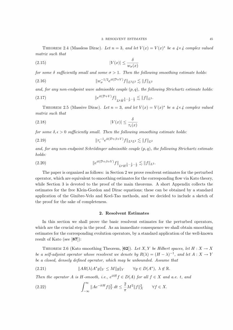
2. RESOLVENT ESTIMATES 45
Theorem 2.4 (Massless Dirac). Let n = 3, and let V (x) = V (x)∗ be a 4×4 complex valuedmatrix such that
(2.15) |V (x)| ≤ δ
wσ(x)
for some δ sufficiently small and some σ > 1. Then the following smoothing estimate holds:
(2.16) ‖w−1/2σ eit(D+V )f‖L2L2 . ‖f‖L2
and, for any non-endpoint wave admissible couple (p, q), the following Strichartz estimate holds:
(2.17) ‖eit(D+V )f‖LpH
1q−
1p−
12
. ‖f‖L2 .
Theorem 2.5 (Massive Dirac). Let n = 3, and let V (x) = V (x)∗ be a 4×4 complex valuedmatrix such that
(2.18) |V (x)| ≤ δ
τε(x)
for some δ, ε > 0 sufficiently small. Then the following smoothing estimate holds:
(2.19) ‖τ−1ε eit(D+β+V )f‖L2L2 . ‖f‖L2
and, for any non-endpoint Schrodinger admissible couple (p, q), the following Strichartz estimateholds:
(2.20) ‖eit(D+β+V )f‖LpH
1q−
1p−
12
. ‖f‖L2 .
The paper is organized as follows: in Section 2 we prove resolvent estimates for the perturbedoperator, which are equivalent to smoothing estimates for the corresponding flow via Kato theory,while Section 3 is devoted to the proof of the main theorems. A short Appendix collects theestimates for the free Klein-Gordon and Dirac equations; these can be obtained by a standardapplication of the Ginibre-Velo and Keel-Tao methods, and we decided to include a sketch ofthe proof for the sake of completeness.
2. Resolvent Estimates
In this section we shall prove the basic resolvent estimates for the perturbed operators,which are the crucial step in the proof. As an immediate consequence we shall obtain smoothingestimates for the corresponding evolution operators, by a standard application of the well-knownresult of Kato (see [87]):
Theorem 2.6 (Kato smoothing Theorem, [62]). Let X,Y be Hilbert spaces, let H : X → X
be a self-adjoint operator whose resolvent we denote by R(λ) = (H − λ)−1, and let A : X → Y
be a closed, densely defined operator, which may be unbounded. Assume that
(2.21) ‖AR(λ)A∗g‖Y ≤M‖g‖Y ∀g ∈ D(A∗), λ 6∈ R.
Then the operator A is H-smooth, i.e., eitHf ∈ D(A) for all f ∈ X and a.e. t, and
(2.22)∫ ∞
−∞‖Ae−itHf‖2
Y dt ≤2πM2‖f‖2
X ∀f ∈ X.

46 2. STRICHARTZ ESTIMATES AND KATO-SMOOTHING EFFECT
2.1. The magnetic Schrodinger operator. The following lemma gives sufficient condi-tions for the magnetic Schrodinger operator H = −(∇ + iA(x))2 + B(x) to be selfadjoint. Wesketch a proof since the assumptions on the coefficients are not completely standard:
Lemma 2.1. Let Aj(x), A = (A1, . . . , An) and B(x) be real valued functions satisfying
(2.23) ‖B+‖Ln/2,∞ < C, ‖B−‖Ln/2,∞ < δ, ‖A‖Ln,∞ < δ
for some C, δ > 0. Then, if δ is sufficiently small, the operator
(2.24) H = −(∇+ iA(x))2 +B(x)
can be uniquely defined as a selfadjoint nonnegative operator in L2, with form domain H1(Rn).Moreover we have
(2.25) ‖H1/2g‖L2 ' ‖g‖H1 .
Proof. The quadratic form
q(φ, ψ) = ((∇+ iA(x))φ, (∇+ iA(x))ψ)L2 + (B(x)φ, ψ)L2
is well defined on H1 × H1 under assumptions (2.23). Indeed, using the embedding H1 ⊂L2n/(n−2),2, Holder’s inequality in Lorentz spaces [80] and assumptions (2.23), we have
|q(ϕ,ϕ)| ≤‖∇ϕ‖2L2 + 2‖A‖Ln,∞‖∇ϕ · ϕ‖
Ln
n−1 ,1 + ‖|A|2 + |B|‖L
n2 ,∞‖ϕ2‖
Ln
n−2 ,1
.‖∇ϕ‖2L2 .
The form q is symmetric since A and B are real valued. By standard results (see e.g. [87],Theorem VIII.15), q is the form associated to a unique defined self-adjoint operator providedthe form is closed, i.e. its domain H1(Rn) is complete under the norm
(2.26) |||ϕ|||2 = q(ϕ,ϕ) + C‖ϕ‖2L2 ,
for some C > 0, and it is semibounded, i.e.
(2.27) q(ϕ,ϕ) ≥ −C‖ϕ‖2L2 ,
for some C > 0. To prove this we estimate the form from below as follows
q(ϕ,ϕ) = ‖∇ϕ‖2L2 + 2=(A · ∇ϕ,ϕ)L2 + ((|A|2 +B+)ϕ,ϕ)L2 − (B−ϕ,ϕ)L2
≥ ‖∇ϕ‖2L2 + 2=(A · ∇ϕ,ϕ)L2 − (B−ϕ,ϕ)L2 .
Proceeding as for the upper bound we obtain
(2.28) q(ϕ,ϕ) ≥ ‖∇ϕ‖2L2 − Cδ‖∇ϕ‖2
L2 & ‖∇ϕ‖2L2
for δ small enough. This proves the semiboundedness of the form and (2.25), which implies thatthe norm (2.26) is equivalent to the norm of H1 and hence the form is closed. �
We now investigate in some detail the properties of the resolvent operators
(2.29) R(z) = (−∆ +W − z)−1
R0(z) = (−∆− z)−1, Rb2(z) = (−∆ + b2(x)− z)−1.
The following weight functions will appear in our resolvent estimates (ε > 0, σ > 1):
(2.30) 〈x〉 = (1 + |x|2)12 , wσ(x) = |x|(1 + | log |x||)σ,

2. RESOLVENT ESTIMATES 47
and
(2.31) τε(x) =
{|x|
12−ε + |x| if n ≥ 3,
|x|12−ε + |x|1+ε if n = 2.
Notice that|x| ≤ τε(x), w
12σ (x) ≤ Cτε(x),
andτε(x) ≤ C〈x〉, for n ≥ 3, τε(x) ≤ C〈x〉1+ε, for n = 2
for some constant C = C(ε, σ).In order to estimate the resolvent R we shall use the formal identity
(2.32) R = R0(I + b2R0)−1(I + (a · ∇+ b1)Rb2)−1.
Our first goal will be to prove that the operators (I + b2R0)−1 and (I + (a · ∇+ b1)Rb2)−1 are
well defined and uniformly bounded in suitable weighted L2 spaces. In the following lemma, theassumption that 0 is not a resonance of −∆ + b(x) means that the only distribution solution fof the equation −∆f + bf = 0 belonging to L2(〈x〉−2dx) is f ≡ 0.
Lemma 2.2. Let b(x) be real valued and such that, for some ε, δ > 0 small enough (recall(2.31)),
(2.33) ‖τ2ε b+‖L∞ <∞, ‖τ2
ε b−‖L∞ < δ.
Assume that 0 is not a resonance for −∆+ b(x). Then I + bR0(z) is invertible with a uniformlybounded inverse on L2(τ2
ε dx):
(2.34) ‖τε(I + bR0(z))−1f‖L2 ≤ C‖τεf‖L2 .
Proof. We recall the following estimates for the free resolvent R0: fix any σ > 1, then forall z ∈ C
(2.35) ‖w−12
σ R0(z)f‖L2 ≤C√|z|‖w
12σ f‖L2 ,
(2.36) ‖w−12
σ ∇R0(z)f‖L2 ≤ C‖w12σ f‖L2 ,
(2.37) ‖ |x|−1R0f‖L2 ≤ C‖ |x|f‖L2 , n ≥ 3
(2.38) ‖ |x|−1+ε|D|εR0f‖L2 ≤ C‖ |x|1−ε|D|−εf‖L2 , n = 2 (0 < ε < 1/2)
(see [6], [31] for (2.35), (2.36), and [65] for (2.37)-(2.38)). As usual, for λ ∈ R+ the resolventR0(z) must be replaced with the limit operators R0(λ ± i0). By the elementary inequalities
|x| ≤ τε(x), w12σ (x) ≤ Cτε(x), we can condense the estimates (2.35) and (2.37) in the following
(weaker) one for n ≥ 3:
(2.39) ‖τ−1ε R0(z)f‖L2 ≤
C√〈z〉‖τεf‖L2 , for all z ∈ C.
In dimension n = 2 we deduce by duality from (2.38) the following
‖ |D|ε|x|−1+εR0f‖L2 ≤ C‖ |D|−ε|x|1−εf‖L2 ,

48 2. STRICHARTZ ESTIMATES AND KATO-SMOOTHING EFFECT
which implies, via Sobolev embedding and Holder inequality,
‖〈x〉−σ|x|−1+εR0f‖L2 ≤ C‖〈x〉σ|x|1−εf‖L2 , σ > ε
and hence (2.39) follows also for n = 2 (recall (2.31))Now, using assumption (2.33), we have
(2.40) ‖τεbR0(z)f‖L2 ≤ ‖τ2ε b‖L∞‖τ−1
ε R0(z)f‖L2 ≤C√〈z〉‖τ2
ε b‖L∞‖τεf‖L2 ,
with C as in (2.39); hence, if z is sufficiently large, namely so large that
〈z〉 > C2‖τ2ε b‖2
L∞ ,
we can invert the operator I + bR0 by a Neumann series in the weighted space L2(τ2ε dx), with
a uniform bound on the norm of the inverse.In the low frequency case
(2.41) 〈z〉 ≤ C2‖τ2ε b‖2
L∞ ,
the family of operators (I+ bR0(z)) is uniformly bounded in L2(τ2ε dx) by (2.40). We also notice
that bR0 is a compact operator on L2(τ2ε dx); indeed, R0 is a compact operator from L2(τ2
ε dx) toL2(τ−2
ε dx) (see (2.35)–(2.36)), while multiplication by b is bounded from L2(τ−2ε dx) to L2(τ2
ε dx).Thus by standard analytic Fredholm theory we can invert I + bR0(z) uniformly in z, providedI + bR0(z) is injective on L2(τ2
ε dx) for each fixed z. This is obvious for z outside R+, since byour assumptions the operator −∆ + b is nonnegative and selfadjoint, and is true by assumptionfor z = 0, hence we need only check the case z = λ > 0.
Thus let λ ≥ 0 and f ∈ L2(τ2ε dx) such that f+b(x)R0(λ+i0)f = 0 (the −i0 case is identical).
We notice that estimate (2.36) implies that R0(z)f ∈ H1loc and hence in particular R0(z)f is
in L2n/(n−2) locally. Since |b| . τ−2ε which is locally in Ln, we conclude that f = −bR0(λ)f
is locally in L2. Recalling that f ∈ L2(τ2ε dx) this implies f ∈ L2(〈x〉2dx). Thus we are in the
framework of the standard Agmon theory and we deduce that λ is an eigenvalue of −∆ + b(x);but this is excluded under our assumptions on b, for instance by the results of [58] (Theorem2.1).
In conclusion, we can invert (I + bR0(z)) in L2(τ2ε dx), for z 6= 0, with an uniform bound for
the inverse (I + bR0)−1, and this completes the proof. �
The preceding lemma allows us to construct the resolvent operator
(2.42) Rb(z) = R0(z)(I + bR0(z))−1,
which, in view of (2.34) and (2.39), is a bounded operator from L2(τ2ε dx) to L2(τ−2
ε dx) for allz ∈ C.
We have next:
Lemma 2.3. Consider the operator −∆ + a(x) · ∇ + b1(x) + b2(x) under the following as-sumptions: the operator is selfadjoint, b2 is real valued and nonnegative, and for some δ, ε > 0small enough, σ > 1,
(2.43) ‖τεw12σ a‖L∞ + ‖τ2
ε b1‖L∞ < δ, ‖τ2ε b2‖L∞ <∞.

2. RESOLVENT ESTIMATES 49
Moreover assume that 0 is not a resonance for −∆+ b2(x). Then I+(a ·∇+ b1)Rb2 is invertiblewith a bounded inverse on L2(τ2
ε dx):
(2.44) ‖τε(I + (a · ∇+ b1)Rb2)−1f‖L2 ≤ C‖τεf‖L2 .
Proof. Using assumptions (2.43), Holder inequality and estimate (2.36), we can write
‖τεa · ∇Rb2f‖L2 ≤ ‖τεa · ∇R0(I + b2R0)−1f‖L2
≤ ‖τεw12σ a‖L∞‖w
− 12
σ ∇R0(I + b2R0)−1f‖L2
. δ · ‖w12σ (I + b2R0)−1f‖L2
. δ · ‖τε(I + b2R0)−1f‖L2
and Lemma 2.2 gives finally
‖τεa · ∇Rb2f‖L2 . δ · ‖τεf‖L2 .
On the other hand, by (2.43) and estimate (2.39)
‖τεb1Rb2f‖L2 ≤ ‖τ2ε b1‖L∞‖τ−1
ε R0(I + b2R0)−1f‖L2
. δ · ‖τε(I + b2R0)−1f‖L2
and again by Lemma 2.2 we have
‖τεb1Rb2f‖L2 . δ · ‖τεf‖L2 .
Thus, if δ is sufficiently small, we can invert I + (a · ∇ + b1)Rb2 via a Neumann series, and weobtain (2.44). �
We collect and complete the above estimates in the following
Proposition 2.2. Consider the operator −∆ + W (x,D) ≡ −∆ + a(x) · ∇ + b1(x) + b2(x)under the assumptions: the operator is selfadjoint, b2 is real valued and nonnegative, and forsome δ, ε > 0 small enough, σ > 1,
(2.45) ‖τεw12σ a‖L∞ + ‖τ2
ε b1‖L∞ < δ, ‖τ2ε b2‖L∞ <∞.
Moreover assume that 0 is not a resonance for −∆+ b2(x). Then the resolvent operator R(z) =(−∆ +W − z)−1 satisfies the following estimates for all z ∈ C:
(2.46) ‖τ−1ε R(z)f‖L2 ≤
C√〈z〉‖τεf‖L2 ,
(2.47) ‖τ−1ε ∇R(z)f‖L2 ≤ C‖τεf‖L2 .
and
(2.48) ‖〈x〉−1R(z)f‖H1 ≤ C‖〈x〉f‖L2 , n ≥ 3;
replace the weights 〈x〉−1, 〈x〉 by 〈x〉−1−ε, 〈x〉1+ε respectively in dimension 2. As a consequence,the Schrodinger flow eit(−∆+W )f has the smoothing property
(2.49) ‖τ−1ε eit(−∆+W )f‖L2L2 + ‖τ−1
ε |D|1/2eit(−∆+W )f‖L2L2 ≤ C‖f‖L2 .

50 2. STRICHARTZ ESTIMATES AND KATO-SMOOTHING EFFECT
Remark 2.1. For the following applications it will be convenient to rewrite the (second)smoothing estimate above in the equivalent form
(2.50) ‖τ−1ε ∇|D|−1/2eit(−∆+W )f‖L2L2 ≤ C‖f‖L2 .
This follows immediately from the fact that ∂j |D|−1/2 = iRj |D|1/2, where Rj = i−1∂j |D|−1 isthe j-th Riesz operator, and on the other hand τ−1
ε is an A2 weight, as proved in Lemma 2.4below.
Proof. Estimates (2.46) and (2.47) are immediate consequences of (2.32), (2.36) and ofLemmas 2.2, 2.3. Moreover, (2.46) implies in particular
‖τ−1ε R(z)f‖L2 ≤ C‖τεf‖L2 ,
and the Kato smoothing theorem with the choices A = τ−1ε , X = Y = L2 gives the first estimate
in (2.49).To prove (2.48), write
‖〈x〉−1Rf‖H1 . ‖〈x〉−1Rf‖L2 + ‖〈x〉−2Rf‖L2 + ‖〈x〉−1∇Rf‖L2
. ‖〈x〉−1Rf‖L2 + ‖〈x〉−1∇Rf‖L2
The first term at the right hand side can be estimated by (2.46)
(2.51) ‖〈x〉−1Rf‖L2 ≤ C‖τ−1ε Rf‖L2 ≤ C‖τεf‖L2 ≤ C‖〈x〉f‖L2 ,
while the third term is bounded using (2.47):
(2.52) ‖〈x〉−1∇Rf‖L2 ≤ ‖τ−1ε ∇Rf‖L2 ≤ C‖τεf‖L2 ≤ C‖〈x〉f‖L2
and this proves (2.48).Now write (2.48) in the equivalent forms
‖〈D〉〈x〉−1R(z)〈x〉−1f‖L2 ≤ C‖f‖L2
and, by duality,‖〈x〉−1R(z)〈x〉−1〈D〉f‖L2 ≤ C‖f‖L2 .
The last two estimates state that the operator 〈x〉−1R(z)〈x〉−1 is bounded, uniformly in z ∈ C,from L2 to H1 and from H−1 to L2. By complex interpolation this implies that it is also boundedfrom H−1/2 to H1/2, i.e.,
‖〈D〉1/2〈x〉−1R(z)〈x〉−1〈D〉1/2f‖L2 ≤ C‖f‖L2
Then by Kato smoothing we obtain also the second estimate in (2.49).The proof for the case n = 2 is completely analogous. �
2.2. The wave and Klein-Gordon generators. We consider now the operator√−∆ +W ,
where as usualW = W (x,D) = a · ∇+ b, b = b1 + b2
which generates the flow eit√−∆+W of the perturbed wave equation. The free operator |D| :=√
−∆ is self-adjoint and nonnegative on L2, and can be handled as follows. If we denote itsresolvent by R|D|(z) = (|D| − z)−1, we have
(2.53) R|D|(z) = (|D|+ z)R0(z2).
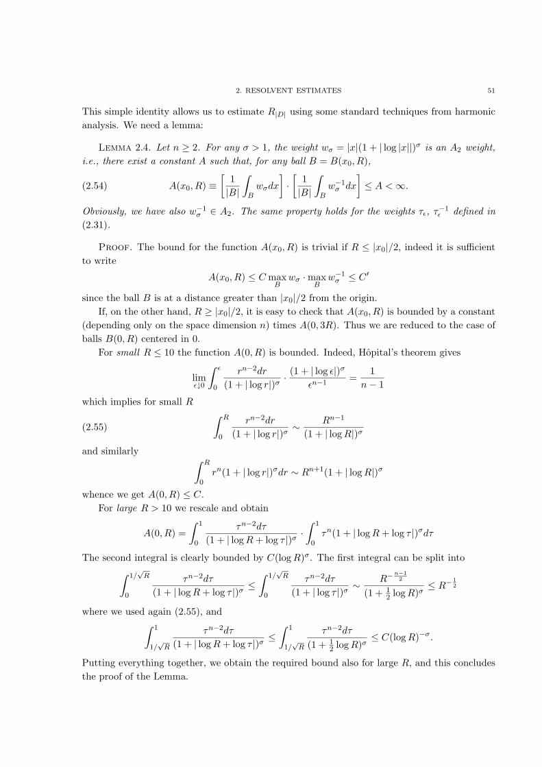
2. RESOLVENT ESTIMATES 51
This simple identity allows us to estimate R|D| using some standard techniques from harmonicanalysis. We need a lemma:
Lemma 2.4. Let n ≥ 2. For any σ > 1, the weight wσ = |x|(1 + | log |x||)σ is an A2 weight,i.e., there exist a constant A such that, for any ball B = B(x0, R),
(2.54) A(x0, R) ≡[
1|B|
∫Bwσdx
]·[
1|B|
∫Bw−1
σ dx
]≤ A <∞.
Obviously, we have also w−1σ ∈ A2. The same property holds for the weights τε, τ−1
ε defined in(2.31).
Proof. The bound for the function A(x0, R) is trivial if R ≤ |x0|/2, indeed it is sufficientto write
A(x0, R) ≤ CmaxB
wσ ·maxB
w−1σ ≤ C ′
since the ball B is at a distance greater than |x0|/2 from the origin.If, on the other hand, R ≥ |x0|/2, it is easy to check that A(x0, R) is bounded by a constant
(depending only on the space dimension n) times A(0, 3R). Thus we are reduced to the case ofballs B(0, R) centered in 0.
For small R ≤ 10 the function A(0, R) is bounded. Indeed, Hopital’s theorem gives
limε↓0
∫ ε
0
rn−2dr
(1 + | log r|)σ· (1 + | log ε|)σ
εn−1=
1n− 1
which implies for small R
(2.55)∫ R
0
rn−2dr
(1 + | log r|)σ∼ Rn−1
(1 + | logR|)σ
and similarly ∫ R
0rn(1 + | log r|)σdr ∼ Rn+1(1 + | logR|)σ
whence we get A(0, R) ≤ C.For large R > 10 we rescale and obtain
A(0, R) =∫ 1
0
τn−2dτ
(1 + | logR+ log τ |)σ·∫ 1
0τn(1 + | logR+ log τ |)σdτ
The second integral is clearly bounded by C(logR)σ. The first integral can be split into∫ 1/√
R
0
τn−2dτ
(1 + | logR+ log τ |)σ≤∫ 1/
√R
0
τn−2dτ
(1 + | log τ |)σ∼ R−
n−12
(1 + 12 logR)σ
≤ R−12
where we used again (2.55), and∫ 1
1/√
R
τn−2dτ
(1 + | logR+ log τ |)σ≤∫ 1
1/√
R
τn−2dτ
(1 + 12 logR)σ
≤ C(logR)−σ.
Putting everything together, we obtain the required bound also for large R, and this concludesthe proof of the Lemma.
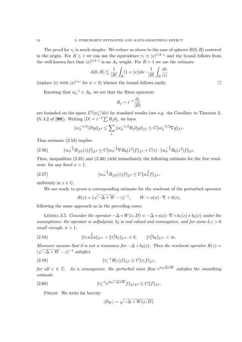
52 2. STRICHARTZ ESTIMATES AND KATO-SMOOTHING EFFECT
The proof for τε is much simpler. We reduce as above to the case of spheres B(0, R) centeredin the origin. For R ≤ 1 we can use the equivalence τε ' |x|1/2−ε and the bound follows fromthe well-known fact that |x|1/2−ε is an A2 weight. For R > 1 we use the estimate
A(0, R) .1|B|
∫B
(1 + |x|)dx · 1|B|
∫B
dx
|x|
(replace |x| with |x|1+ε for n = 2) whence the bound follows easily. �
Knowing that w−1σ ∈ A2, we see that the Riesz operators
Rj = i−1 ∂j
|D|
are bounded on the space L2(w−1σ dx) by standard results (see e.g. the Corollary to Theorem 2,
§V.4.2 of [99]). Writing |D| = i−1∑Rj∂j , we have
‖w−1/2σ |D|g‖L2 ≤
∑j
‖w−1/2σ Rj∂jg‖L2 ≤ C‖w−1/2
σ ∇g‖L2 .
Thus estimate (2.53) implies
(2.56) ‖w−12
σ R|D|(z)f‖L2 ≤ C‖w−12
σ ∇R0(z2)f‖L2 + C|z| · ‖w−12
σ R0(z2)f‖L2 .
Then, inequalities (2.35) and (2.36) yield immediately the following estimate for the free resol-vent: for any fixed σ > 1,
(2.57) ‖w−12
σ R|D|(z)f‖L2 ≤ C‖w12σ f‖L2 ,
uniformly in z ∈ C.We are ready to prove a corresponding estimate for the resolvent of the perturbed operator
R(z) = (√−∆ +W − z)−1, W = a(x) · ∇+ b(x),
following the same approach as in the preceding cases.
Lemma 2.5. Consider the operator −∆+W (x,D) ≡ −∆+a(x) ·∇+b1(x)+b2(x) under theassumptions: the operator is selfadjoint, b2 is real valued and nonnegative, and for some δ, ε > 0small enough, σ > 1,
(2.58) ‖τεw12σ a‖L∞ + ‖τ2
ε b1‖L∞ < δ, ‖τ2ε b2‖L∞ <∞.
Moreover assume that 0 is not a resonance for −∆+ b2(x). Then the resolvent operator R(z) =(√−∆ +W − z)−1 satisfies
(2.59) ‖τ−1ε R(z)f‖L2 ≤ C‖τεf‖L2 ,
for all z ∈ C. As a consequence, the perturbed wave flow eit√
∆+W satisfies the smoothingestimate
(2.60) ‖τ−1ε eit
√−∆+W f‖L2L2 ≤ C‖f‖L2 .
Proof. We write for brevity
|DW | =√−∆ +W (x,D).
2. RESOLVENT ESTIMATES 53
By the (Phragmen-Lindelof) maximum principle, it is sufficient to prove estimate (2.59) for realz = λ. We notice that by the same arguments used in the proof of Lemma 2.1, we have
‖|DW |g‖L2 ' ‖g‖H1 ;
thus for λ ≤ 0 we can write
‖(|DW | − λ)g‖2L2 = ‖|DW |g‖2
L2 + λ2‖g‖2L2 − 2λ(|DW |g, g)L2 & ‖g‖H1
by the nonnegativity of |DW |. This implies for all λ ≤ 0
‖R(λ)g‖H1 . ‖g‖L2 ,
whence by duality we have also‖R(λ)g‖L2 . ‖g‖H−1 ,
and interpolating we obtain
‖R(λ)g‖H1/2 . ‖g‖H−1/2 , λ ≤ 0.
Now, using the Hardy’s inequalities
‖|x|−1/2f‖L2 . ‖f‖H1/2 or equivalently ‖f‖H−1/2 . ‖|x|1/2f‖L2
we obtain the estimate
(2.61) ‖|x|−1/2R(λ)g‖L2 . ‖|x|1/2g‖L2 , λ ≤ 0
which implies (2.59) for z = −λ ≤ 0 (and is actually stronger).Consider now R(λ), λ ≥ 0; we use the identity
R(λ) = (|DW | − λ)−1 = 2λRW (λ2) + (|DW |+ λ)−1
where RW (λ) = (−∆ + W − λ)−1. The second term at the right hand side has already beenestimated, while the first one can be estimated using (2.46), and this concludes the proof of(2.59). The last inequality (2.60) is an application of Kato’s theorem as usual. �
We conclude this section with a study of the operator√−∆ + 1 +W associated with the
perturbed Klein-Gordon flow eit√−∆+1+W . In the free case W = 0 the operator reduces to
〈D〉 = (1−∆)1/2 and its resolvent
R〈D〉(z) = (〈D〉 − z)−1
can be handled in a similar way as R|D|.We start from estimates (2.36) and (2.39) which imply
〈z〉1/2‖τ−1ε R0(z)f‖L2 + ‖w−1/2
σ ∇R0(z)f‖L2 . ‖τεf‖L2 .
As above, using the fact that w−1σ is an A2 weight, we can replace ∇ with |D| in the left hand
side and hence (recalling that w12σ . τε) we arrive at
(2.62) 〈z〉1/2‖τ−1ε R0(z)f‖L2 + ‖τ−1
ε 〈D〉R0(z)f‖L2 . ‖τεf‖L2 .
Then using the identityR〈D〉(z) = (〈D〉+ z) ·R0(1− z2)
we obtain from (2.62) the estimate
(2.63) ‖τ−1ε R〈D〉(z)f‖L2 . ‖τεf‖L2 .
54 2. STRICHARTZ ESTIMATES AND KATO-SMOOTHING EFFECT
For the perturbed operator we have:
Lemma 2.6. Consider the operator −∆+W (x,D) ≡ −∆+a(x) ·∇+b1(x)+b2(x) under theassumptions: the operator is selfadjoint, b2 is real valued and nonnegative, and for some δ, ε > 0small enough, σ > 1,
(2.64) ‖τεw12σ a‖L∞ + ‖τ2
ε b1‖L∞ < δ, ‖τ2ε b2‖L∞ <∞.
Moreover assume that 0 is not a resonance for −∆+ b2(x). Then the resolvent operator R(z) =(√
1−∆ +W − z)−1 satisfies
(2.65) ‖τ−1ε R(z)f‖L2 ≤ C‖τεf‖L2 .
As a consequence, the perturbed Klein-Gordon flow eit√
∆+1+W satisfies the smoothing estimate
(2.66) ‖τ−1ε eit
√−∆+1+W f‖L2L2 ≤ C‖f‖L2 .
Proof. Writing
|DW | =√−∆ +W (x,D), 〈DW 〉 =
√1−∆ +W (x,D)
we notice that‖〈DW 〉f‖L2 ' ‖f‖L2 + ‖|DW |f‖L2 ' ‖f‖H1
by the same arguments used in the proof of Lemma 2.1 and the identity
‖〈DW 〉f‖2L2 = ((1−∆ +W )f, f).
Proceeding as in the proof of Lemma 2.5, we arrive at
‖R(λ)g‖H1/2 . ‖g‖H−1/2 , λ ≤ 0
for the resolvent R = (〈DW 〉 − z)−1, and by Hardy inequality as before we obtain half of(2.66).For positive λ we write
R(λ) = (〈DW 〉 − λ)−1 = 2λRW (λ2 − 1) + (〈DW 〉+ λ)−1
where RW (z) = (−∆+W − z)−1, and by (2.46) and the first part of the proof we obtain (2.65).Kato’s theorem gives (2.66) as usual. �
2.3. The magnetic Dirac operators. We now consider the resolvent of a perturbed Diracoperator D + V (x). The proofs here will be short since we shall rely on a few results proved in[31]; in particular, we recall that if V = V ∗ has a sufficiently small L3,∞ norm, hence under theassumptions of Theorem 2.4, the operator D+V is self-adjoint on L2(R3,C4), with form domainH1(R3,C4) and spectrum R. The same holds for the operator with nonzero mass D + β + V ,but the spectrum is R\]− 1, 1[.
Let us consider the massless case first. We shall use the notations
(2.67) RD(z) = (−D − zI4)−1, R(z) = (−D + V − zI4)−1
where I4 denotes the identity 4× 4-matrix. The following result is contained in Proposition 3.6of [31], apart from the smoothing estimate which is a standard consequence of Kato’s theoremas above:
2. RESOLVENT ESTIMATES 55
Proposition 2.3. Assume that the 4× 4 matrix V (x) = V ∗(x) satisfies
(2.68) ‖wσV ‖L∞ < δ,
for some δ sufficiently small and some σ > 0. Then D + V satisfies the limiting absorptionprinciple, i.e., the limit operators R(λ ± i0) exist in the topology of bounded operators fromL2(w1/2
σ dx) to H1(w1/2σ dx). Moreover the resolvent operator R = (−D+V − zI4)−1 satisfies the
estimate
(2.69) ‖w−1/2σ R(z)f‖L2 ≤ C‖w1/2
σ f‖L2 , z ∈ C.
As a consequence, the Dirac flow satisfies the smoothing estimate
(2.70) ‖w−1/2σ eit(D+V )f‖L2L2 ≤ C‖f‖L2 .
We consider now the operators with mass D+ β and D+ β+ V . We shall use the notations
Rβ(z) = (D + β − zI4)−1, R(z) = (D + β + V − zI4)−1.
From the identitiesD2 = −∆I4, (D + β)2 = (1−∆)I4,
we obtain the following representations in terms of R0(z) = (−∆− z)−1
RD(z) = R0(z2)(D + zI4), Rβ(z) = R0(z2 − 1)(D + β + zI4);
and hence we can write
(2.71) Rβ(z) = R0(z2 − 1)D +R0(z2 − 1)(β + zI4).
Then a straightforward application of estimate (2.62) gives
(2.72) ‖τ−1ε Rβ(z)f‖L2 ≤ C‖τεf‖L2 .
uniformly in z ∈ C.In the perturbed case we can prove
Proposition 2.4. Assume that the 4× 4 matrix V (x) = V ∗(x) satisfies
(2.73) ‖τ2ε V ‖L∞ < δ,
for some δ sufficiently small and ε > 0. Then the perturbed resolvent operator R(z) = (D+ β +V − zI4)−1 satisfies
(2.74) ‖τ−1ε R(z)f‖L2 ≤ C‖τεf‖L2 .
As a consequence, the flow eit(D+β+V ) satisfies the smoothing estimate
(2.75) ‖τ−1ε eit(D+β+V )f‖L2L2 ≤ C‖f‖L2 .
Proof. The operator V Rβ(z) is bounded on L2(τ2ε dx) with norm bounded by Cδ since
‖τεV Rβ(z)‖L2 ≤ ‖τ2ε V ‖L∞‖τ−1
ε Rβ(z)‖L2 ≤ Cδ‖τεf‖L2
by (2.73) and (2.72). Thus for δ small a Neumann expansion shows that (I +V Rβ(z))−1 is welldefined and uniformly bounded on L2(τ2
ε dx). Hence the usual representation
R(z) = Rβ(z)(I + V Rβ(z))−1
together with (2.72) gives (2.74), and (2.75) follows. �

56 2. STRICHARTZ ESTIMATES AND KATO-SMOOTHING EFFECT
3. Proof of the Strichartz Estimates
The method we shall follow is inspired by [90], [17] and consists in mixing Strichartz andsmoothing estimates for the free operator with smoothing estimates for the perturbed operator.The main tool will be the well-known Christ-Kiselev lemma [22], which can be stated as follows:given two Banach spaces X,Y and a bounded integral operator Tf =
∫RK(t, s)f(s)ds from
Lp(R, X) to Lp(R, Y ), then its truncated version Sf =∫ t0 K(t, s)f(s)ds is also bounded on the
same spaces, provided p < p (the Hilbert transform being a trivial counterexample for p = p).Thus to prove an estimate of the form∥∥∥∥∫ t
0ei(t−s)AF (s)ds
∥∥∥∥Lp
t Lqx
. ‖F‖Lp
t Lqx
it is sufficient to prove the untruncated estimate∥∥∥∥∫Rei(t−s)AF (s)ds
∥∥∥∥Lp
t Lqx
. ‖F‖Lp
t Lqx
but only if p < p, which in particular excludes endpoint-endpoint estimates where p = p = 2.
3.1. Schrodinger equation: proof of Theorem 2.1. Notice that u(t, x) = eit(−∆+W )f
satisfies the equation iut −∆u = −Wu, hence we can write
eit(∆−W )f = eit∆f −∫ t
0ei(t−s)∆W (x,D)u ds = I − II − III
with
I = eit∆f, II =∫ t
0ei(t−s)∆b(x)u ds, III =
∫ t
0ei(t−s)∆a(x) · ∇u ds.
The first term I can be estimated directly with standard Strichartz estimates:
(2.76) ‖eit∆f‖Lpt Lq
x≤ C‖f‖L2
for any admissible couple (p, q). In order to estimate the second term we resort to the Christ-Kiselev lemma and we are reduced to estimate the untruncated integral
II1 = eit∆∫e−is∆b(x)u ds.
To this end we apply first the Strichartz estimates for the free group, then the dual of thesmoothing estimate from Proposition 2.2 in the special case W = 0, i.e.,∥∥∥∥∫ e−is∆F (s)ds
∥∥∥∥L2
. ‖τεF‖L2L2
obtaining
‖II1‖LpLq .
∥∥∥∥∫ e−is∆bu ds
∥∥∥∥L2
. ‖τεbu‖L2L2 ≤ ‖τ2ε b‖L∞‖τεu‖L2L2 .
Then by assumption (2.45) and again the smoothing estimate (2.49) we conclude
(2.77) ‖II‖LpLq . ‖f‖L2
for any non-endpoint admissible couple (p, q).The last term III is more delicate. We reduce it as above to the untruncated form
III1 = eit∆∫e−is∆a · ∇u ds

3. PROOF OF THE STRICHARTZ ESTIMATES 57
and we apply to it the free Strichartz estimate and then the following dual smoothing estimate:
(2.78)∥∥∥∥∫ e−is∆F (s)ds
∥∥∥∥L2
. ‖|D|−1/2χF‖L2L2 ,
valid for any function χ(x) & wσ(x)1/2. Estimate (2.78) is proved as follows: from (2.36) wededuce, using the fact that wσ is an A2 weight, the equivalent property
‖w−1/2σ |D|1/2R0(z)f‖L2 ≤ C‖w1/2
σ |D|−1/2f‖L2
which implies, via Kato smoothing,
‖w−1/2σ |D|1/2eit∆f‖L2L2 ≤ ‖f‖L2 .
Since χ & w1/2σ this gives also
‖χ−1|D|1/2eit∆f‖L2L2 ≤ ‖f‖L2
and by duality we get (2.78). Thus we arrive at
(2.79) ‖III1‖LpLq . ‖|D|−1/2χa(x) · ∇u‖L2L2
Now assume we can prove the inequality
(2.80) ‖|D|−1/2χa(x) · ∇g‖L2 . ‖τ−1ε ∇|D|−1/2g‖L2 ;
then from (2.79) and the smoothing estimate (2.50) we finally obtain
(2.81) ‖III1‖LpLq . ‖τ−1ε ∇|D|−1/2u‖L2 . ‖f‖L2
which, together with (2.76) and (2.77), concludes the proof of the Theorem.It remains to check inequality (2.80). We rewrite it in the equivalent form
‖|D|−1/2χa(x)|D|1/2τεh‖L2 . ‖h‖L2 ,
i.e., we need to prove that the operator
(2.82) T = |D|−1/2χa(x)|D|1/2τε
is bounded on L2. We shall use the following lemma, where we shall make use of severalproperties of Lorentz spaces Lp,q (see [80]).
Lemma 2.7. Let α(x), β(x) be measurable functions on Rn such that for some 0 < δ < 1/2,some ρ ∈ [0, n/2− δ[, and a radial function γ(|x|), with γ(s) decreasing, we have
(i) |α(x)− α(y)| . |x− y|1/2+δ(γ(|x|) + γ(|y|)) and γ ∈ L2n
1+2ρ+2δ,∞
(ii) αβ ∈ L∞, |x|−ρβ(x) ∈ L∞ and |x|ργ(|x|) ∈ L2n
1+2δ,∞
Then the operator T = |D|−1/2α(x)|D|1/2β(x) is bounded on L2.The same result holds in the range ρ ∈ [0, n/2 + δ[ if we replace (i) with(i’) |α(x)− α(y)| ≤ 〈x− y〉−2δ|x− y|1/2+δ(γ(|x|) + γ(|y|)) and γ ∈ L
2n1+2ρ−2δ
,∞.
Proof. Since αβ is bounded, we can equivalently prove that the modified operator
T = T − αβ = |D|−1/2 · [α, |D|1/2] · β
is bounded on L2. Moreover, by the Sobolev embedding in Lorentz spaces (proved e.g. by realinterpolation)
‖|D|−1/2g‖L2 . ‖g‖L
2nn+1 ,2
58 2. STRICHARTZ ESTIMATES AND KATO-SMOOTHING EFFECT
it is sufficient to prove that the following reduced operator S satisfies
S = [α, |D|1/2] · β : L2n
n+1,2 → L2.
Now we observe that the commutator [α, |D|1/2] admits an explicit representation of the form
[α, |D|1/2]f = c(n)∫
Rn
α(x)− α(y)|x− y|n+1/2
f(y)dy
for a constant c(n) depending only on the space dimension. Indeed, by standard Fourier trans-form techniques we see that
[α, |D|z]f = c(z)∫
Rn
α(x)− α(y)|x− y|n+z
f(y)dy
and this formula is valid for <z < 0 under quite general assumptions on α; moreover ourassumptions show that the right hand side is a well defined and analytic function of z for<z < 1/2 + δ (as proved below), hence by analytic continuation the representation is valid alsoin this larger region and in particular for z = 1/2.
In order to estimate S we split it as S = S1 + S2 with
S1f = c
∫|y|≥2|x|
α(x)− α(y)|x− y|n+1/2
β(y)f(y)dy
S2f = c
∫|y|≤2|x|
α(x)− α(y)|x− y|n+1/2
β(y)f(y)dy
In the region |y| ≥ 2|x| we deduce by assumption (i) that
|α(x)− α(y)| ≤ 2|x− y|1/2+δγ(|x|)
since γ is decreasing; moreover we have |x− y| ' |y|, hence∣∣∣∣α(x)− α(y)|x− y|n+1/2
β(y)f(y)∣∣∣∣ . γ(|x|) |β(y)|
|y|ρ|f(y)|
|x− y|n−ρ−δ. γ(|x|) |f(y)|
|x− y|n−ρ−δ
using (ii). Thus, by Holder inequality in Lorentz spaces, we get
‖S1f‖L
2nn+1 ,2 . ‖γ‖
L2n
1+2ρ+2δ,∞
∥∥∥∥∫ |f(y)||x− y|n−ρ−δ
dy
∥∥∥∥L
2nn−2ρ−2δ
,2
(provided ρ < n/2− δ) and by (i) and Young inequality we arrive at
‖S1f‖L
2nn+1 ,2 . ‖|y|−n+ρ+δ‖
Ln
n−ρ−δ,∞‖f‖L2
which concludes. the estimate of the first piece S1.In the region |y| ≤ 2|x|, on the other hand, we can write∣∣∣∣α(x)− α(y)
|x− y|n+1/2β(y)f(y)
∣∣∣∣ . |β(y)||y|ρ
|y|ρ|γ(|y|/2)f(y)||x− y|n−δ
.|y|ρ|γ(|y|/2)f(y)|
|x− y|n−δ
so that by Young inequality
‖S2f‖L
2nn+1 ,2 .
∥∥∥∥∫ |y|ρ|γ(|y|/2)f(y)||x− y|n−δ
∥∥∥∥L
2nn+1 ,2
. ‖|y|δ−n‖L
nn−δ
,∞‖γ|y|ρf‖L
2nn+1+2δ
,2
and by Holder inequality we get
‖S2f‖L
2nn+1 ,2 . ‖|y|ργ‖
L2n
1+2δ,∞‖f‖L2
and this concludes the proof under assumptions (i)-(ii).

3. PROOF OF THE STRICHARTZ ESTIMATES 59
The case of assumptions (i’)-(ii) is almost identical. No change is necessary in the estimateof S2f , while for S1f it is sufficient to write
‖S1f‖L
2nn+1 ,2 . ‖γ‖
L2n
1+2ρ−2δ,∞
∥∥∥∥∫ |f(y)||x− y|n−ρ+δ
dy
∥∥∥∥L
2nn−2ρ+2δ
,2
which is true if ρ < n/2 + δ, and then proceed as above. �
Notice that if we restrict to the special choice β = |x|ρ, γ(x) = 〈x〉−λ, α(x) = χ(x)a(x), thefollowing conditions imply that (i), (ii), (i’) are all satisfied:
(2.83) 0 < δ <12, 0 ≤ ρ <
n
2+ δ, λ ≥ 1
2+ ρ+ δ
and
(2.84) 〈x〉λχ(x)a(x) ∈ C1/2+δ
(recall that ‖f‖Cµ = ‖f‖L∞ + supx 6=y |x − y|−µ|f(x) − f(y)|). All conditions in (i), (ii), (i’)are trivial to check apart from Holder continuity; actually we shall now see that the followingstronger inequality holds:
(2.85) |α(x)− α(y)| . min{1, |x− y|}1/2+δ(〈x〉−λ + 〈y〉−λ).
Indeed, when |x − y| ≥ 1 condition (2.85) follows from 〈x〉λχ(x)a(x) ∈ L∞ which is containedin (2.84). When |x− y| ≤ 1, we write
|α(x)− α(y)| ≤ A+B,
where
A = χ(x)a(x)〈x〉λ|〈x〉−λ − 〈y〉−λ|,
and
B = 〈y〉−λ|〈x〉λχ(x)a(x)− 〈y〉λχ(y)a(y)|.
Then we have directly from (2.84)
B . 〈y〉−λ|x− y|1/2+δ ≤ (〈x〉−λ + 〈y〉−λ)|x− y|1/2+δ
while for A we use the elementary inequality
|〈x〉−λ − 〈y〉−λ| . supξ∈[x,y]
|∇〈z〉−λ|z=ξ · |x− y| . (〈x〉−λ + 〈y〉−λ)|x− y|1/2+δ
together with the bound 〈x〉λχ(x)a(x) ∈ L∞.We can finally apply the lemma to the operator (2.82); since τε = |x|1/2−ε + |x| for n ≥ 3
and τε = |x|1/2−ε + |x|1+ε for n = 2, by the above computation it is sufficient to check conditions(2.83), (2.84) for ρ = 1/2 − ε and ρ = 1 (ρ = 1/2 − ε and ρ = 1 + ε in dimension 2). Wesee that the choices δ = 2ε and λ = 1 + 3ε work in all cases, thus it is sufficient to assume〈x〉1+3εχ(x)a(x) ∈ C1/2+2ε i.e. assumption (2.9). The proof is concluded.

60 2. STRICHARTZ ESTIMATES AND KATO-SMOOTHING EFFECT
3.2. Wave and Klein-Gordon equations: proof of Theorems 2.2, 2.3. Since u(t, x) =eit√−∆+W f solves the Cauchy problem
(2.86)
utt −∆u = −Wuu(0, x) = f(x)ut(0, x) = i
(√−∆ +W
)f(x),
we have the alternative representation
(2.87) eit√−∆+W f = cos(t|D|)f + i
sin(t|D|)|D|
√−∆ +Wf −
∫ t
0
sin((t− s)|D|)|D|
Wuds.
The first two terms satisfy the standard Strichartz estimates for the free wave equation (see(2.2) in the Introduction, and recall also (2.25)). For the third term we apply as usual theChrist-Kiselev lemma and we are reduced to the untruncated integral∫
sin((t− s)|D|)|D|
Wuds = I + II
where, writing c(x) = −∇ · a+ b1 + b2,
I =∫
sin((t− s)|D|)|D|
∇ · (a(x)u)ds, II =∫
sin((t− s)|D|)|D|
c(x)uds.
Consider I; clearly, it is sufficient and actually stronger to estimate the integral
I1 = |D|−1eit|D|∫e−is|D|∇ · (a(x)u)ds = |D|−1∇ · eit|D|
∫e−is|D|a(x)uds.
To this end we recall the standard Strichartz estimate
(2.88) ‖eit|D|f‖LpH
1q−
1p−
12
q
. ‖f‖L2
valid for any wave admissible couple (p, q). Moreover, the smoothing estimate (2.60) holds alsoin the free case W ≡ 0
(2.89) ‖τ−1ε eit|D|f‖L2L2 . ‖f‖L2
and by duality is equivalent to
(2.90)∥∥∥∥∫ e−is|D|F (s)ds
∥∥∥∥L2
. ‖τεF‖L2L2 .
Applying (2.88) and (2.90) to I1 we obtain, since the Riesz operators are bounded in all Lp with1 < p <∞,
‖I1‖LpH
1q−
1p−
12
q
. ‖τεa(x)u‖L2L2 ≤ ‖τ2ε a(x)‖L2‖τ−1
ε u‖L2L2 .
Using again the smoothing estimate (2.60) and assumption (2.11), we conclude
‖I1‖LpH
1q−
1p−
12
q
. ‖f‖L2 .
Consider now the second term II, or more generally
II1 = eit|D|∫|D|−1e−is|D|c(x)uds.
Proceeding as in [18], we shall use the following estimate from [8] (see also [56])
‖|x|−1|D|−1eit|D|f‖L2L2 . ‖f‖H−1/2

3. PROOF OF THE STRICHARTZ ESTIMATES 61
in the dual form:
(2.91)∥∥∥∥∫ |D|−1e−is|D|F (s)ds
∥∥∥∥H1/2
. ‖|x|F‖L2L2 .
Then, applying the Strichartz estimate for the wave equation (2.88) in the form
‖eit|D|f‖LpH
1q−
1p
q
. ‖f‖H
12
followed by (2.91), we obtain
‖II1‖LpH
1q−
1p−
12
q
. ‖|x|c(x)u‖L2L2 . ‖|x|τεc(x)‖L∞‖τ−1ε u‖L2L2 .
Recalling assumption (2.11) and the smoothing estimate (2.60) we finally obtain
‖II1‖LpH
1q−
1p−
12
q
. ‖f‖L2
which concludes the proof of Theorem 2.2.The proof of Theorem 2.3 is completely analogous, using the Strichartz estimate for the free
equation‖eit〈D〉f‖
LpH1q−
1p−
12
q
. ‖f‖L2 ,
which is valid for all Schrodinger admissible couple (p, q), and the following estimate from [8]:
‖〈x〉−1eit〈D〉f‖L2L2 . ‖f‖L2
which implies by duality ∥∥∥∥∫ e−is〈D〉F (s)ds∥∥∥∥
L2
. ‖〈x〉F‖L2L2
and hence also ∥∥∥∥∫ 〈D〉−1e−is〈D〉F (s)ds∥∥∥∥
H1/2
. ‖〈x〉F‖L2L2 .
This estimate replaces (2.91) in the above computation.
3.3. Dirac equation: proof of Theorems 2.4, 2.5. As proved in the Appendix, theStrichartz estimate for the free massless Dirac equation is the following:
(2.92) ‖eitDf‖LpH
1q−
1p−
12
q
. ‖f‖L2
for any wave admissible couple (p, q). On the other hand, as a special case of the smoothingestimate (2.70), we have
(2.93) ‖w−12
σ eitDf‖L2L2 . ‖f‖L2
and by duality we obtain
(2.94)∥∥∥∥∫ e−isDF (s)ds
∥∥∥∥L2
. ‖w12σF‖L2L2 .
Consider now the perturbed Dirac flow u = eit(D+V )f . An alternative representation of u isthe following:
(2.95) u(t, x) = eitDf − eitD∫ t
0e−isDV u(s)ds.

62 2. STRICHARTZ ESTIMATES AND KATO-SMOOTHING EFFECT
The term eitDf satisfies the free Strichartz estimates (2.97); in order to estimate the Duhamelterm as usual we apply the Christ-Kiselev lemma and switch to the untruncated integral. Then,using (2.20), (2.94) and Holder inequality, we have∥∥∥∥eitD ∫ e−isDV uds
∥∥∥∥LpH
1q−
1p−
12
q
.
∥∥∥∥∫ e−isDV uds
∥∥∥∥L2
. ‖w12σ V u‖L2L2 ≤ ‖wσV ‖L∞ · ‖w
− 12
σ u‖L2L2 .(2.96)
Recalling the smoothing estimate (2.70) we obtain∥∥∥∥eitD ∫ e−isDV uds
∥∥∥∥LpH
1q−
1p−
12
q
. ‖f‖L2
and this completes the proof of 2.4.The proof of Theorem 2.5 is completely analogous.
4. Strichartz estimates for the free flows: an Appendix
Strichartz estimates for the free Schrodinger and wave equations are well known, see theIntroduction for the precise statements. It is less easy to find in the literature optimal resultsfor Klein-Gordon and Dirac equations. Hence we devote this appendix to a quick proof of theestimates in these cases.
The massless Dirac flow is trivial since it can be reduced to the wave equation:
Proposition 2.5. Let n = 3. The following Strichartz estimates hold:
(2.97) ‖eitDf‖LpH
1q−
1p−
12
q
. ‖f‖L2
for any wave admissible couple (p, q).
Proof. By the identity
(i∂t +D)(i∂t −D) = −�I4,
we obtain that u(t, x) = eitDf satisfies the Cauchy problem
(2.98)
utt −∆I4u = 0u(0, x) = f(x)ut(0, x) = iDf(x)
and hence each component of u satisfies the same Strichartz estimates as for the 3D waveequation. �
The Klein-Gordon and massive Dirac equations need some work. We begin by the free Klein-Gordon flow u = eit〈D〉f . We shall apply a precise stationary phase result due to Hormander[55]:
Lemma 2.8. Assume that φ : Rn → R has a Fourier transform φ ∈ C∞ with the decayproperty
(2.99)∣∣∣Dαφ(ξ)
∣∣∣ ≤ Cα〈ξ〉−n2−1−|α| ∀ξ ∈ Rn, α ∈ Nn.

4. STRICHARTZ ESTIMATES FOR THE FREE FLOWS: AN APPENDIX 63
Then the following estimate holds: for some C > 0,
(2.100)∣∣∣eit〈D〉φ∣∣∣ ≤ C(|t|+ |x|)−
n2 .
Now, using an inhomogeneous dyadic decomposition {ψ0, ϕj(D)}j≥1 with the usual proper-ties: ψ0(ξ) supported in B(0, 1), ϕ0(ξ) = ψ0(ξ/2)− ψ0(ξ),
ϕj(ξ) = ϕ0(2−jξ), ψ0 +∑j≥1
ϕj = 1
we can localize the estimate as follows:
Lemma 2.9. The flow eit〈D〉f satisfies the localized dispersive estimate
(2.101) |eit〈D〉ϕj(D)f | ≤ C|t|−n2 2j(n
2+1)‖ϕj(D)f‖L1 ,
for each t ∈ R, x ∈ Rn, j ≥ 0 and some C > 0; here ϕj denotes ϕj−1 +ϕj +ϕj+1, with ϕ−1 = 0.
Proof. We can write
eit〈D〉ϕj(D)f = eit〈D〉〈D〉−n2−1〈D〉
n2+1ϕj(D)f = eit〈D〉F−1
(〈ξ〉−
n2−1)∗ (ϕj(D)f) ,
where F−1 denotes the inverse Fourier transform. Then, applying Lemma 2.8 with φ =F−1
(〈ξ〉−
n2−1), we obtain
(2.102)∣∣∣eit〈D〉ϕj(D)f
∣∣∣ ≤ C|t|−n2 ‖〈D〉
n2+1ϕj(D)f‖L1 .
Since〈D〉
n2+1ϕj(D)f = F−1
(〈ξ〉
n2+1ϕj(ξ)
)∗ f,
Young inequality gives
(2.103) ‖〈D〉n2+1ϕj(D)f‖L1 ≤ ‖F−1
(〈ξ〉
n2+1ϕj(ξ)
)‖L1‖f‖L1 .
Notice that we can replace in this computation f with ϕj(D)f since ϕj(D)ϕj(D) = ϕj(D).Thus to conclude the proof it is sufficient to get the following estimate:
(2.104) ‖F−1(〈ξ〉
n2+1ϕj(ξ)
)‖L1 ≤ C2j(n
2+1).
Using the scaling operators Sλφ(x) = φ(λx), we can write
F−1(〈ξ〉
n2+1ϕj(ξ)
)= F−1
(〈ξ〉
n2+1S2−jϕ0(ξ)
)= 2j(n
2+1)2jnS2jF−1
((2−2j + |ξ|2)
n2+1ϕ0(ξ)
)and hence
‖F−1(〈ξ〉
n2+1ϕj(ξ)
)‖L1 ≤ 2j(n
2+1)‖F−1
((2−2j + |ξ|2)
n2+1ϕ0(ξ)
)‖L1 .
Moreover, multiplying and dividing by 〈x〉2m for some integer m, we obtain
‖F−1((2−2j + |ξ|2)
n2+1ϕ0(ξ)
)‖L1 ≤ C‖〈x〉2mF−1
((2−2j + |ξ|2)
n2+1ϕ0(ξ)
)‖L2
= C‖(1−∆)m((2−2j + |ξ|2)
n2+1ϕ0(ξ)
)‖L2 ,(2.105)
provided
(2.106) m >n
4.
64 2. STRICHARTZ ESTIMATES AND KATO-SMOOTHING EFFECT
We shall choose m as the smallest integer satisfying (2.106). We are interested in the growthwith respect to j of the quantity
I := (1−∆)m((2−2j + |ξ|2)
n2+1ϕ0(ξ)
).
When n is even,(2−2j + |ξ|2
)n2+1 is a polynomial, and hence we obtain
‖I‖L2 ≤ C‖ϕ0‖L2
with C independent of j. When n is odd, it is clear that almost all the terms in the expansionof I are uniformly bounded in j, apart from the (possibly) worst one
II = ∆m(2−2j + |ξ|2
)n2+1.
We have the two possibilities
n = 4k + 3 or n = 4k + 1,
with m = k + 1. If n = 4k + 3, we have
|II| '∣∣∣D2k+2
((2−2j + |ξ|2)2k+ 5
2
)∣∣∣which expands in a sum of bounded terms. If n = 4k + 1, we have
|II| '∣∣∣D2k+2
((2−2j + |ξ|2)2k+ 3
2
)∣∣∣ . (2−2j + |ξ|2)−1/2 |ξ|2k+2 + bounded terms,
and also in this case we have a uniform bound in j. In conclusion, we have proved that
‖(1−∆)m((2−2j + |ξ|2)
n2+1ϕ0(ξ)
)‖L2 ≤ C,
for some C > 0, which implies (2.104), and the proof is complete. �
Remark 2.2. By interpolation between estimate (2.101) and the localized L2 conservation
(2.107) ‖eit〈D〉ϕj(D)f‖L2 ≤ ‖ϕj(D)f‖L2 ,
we obtain the following Lq − Lq′ decay estimates:
(2.108) ‖eit〈D〉ϕj(D)f‖Lq ≤ C|t|−n2+n
q 2j(n2+1)(1− 2
p)‖ϕj(D)f‖Lq′
for any q ≥ 2 with 1/q + 1/q′ = 1.
Starting from estimates (2.108) and using the standard techniques of [47], [66], in particularthe abstract Theorem 10.1 of [66], we obtain the full set of estimates including the endpointcase:
Theorem 2.7. The Klein-Gordon flow u = eit〈D〉f satisfies the Strichartz estimates
(2.109) ‖eit〈D〉f‖LpH
1q−
1p−
12
q
. ‖f‖L2
for any Schrodinger admissible couple (p, q).
Finally, the Dirac equation with mass can be handled in a similar way to Proposition 2.5:
Proposition 2.6. Let n = 3. The following Strichartz estimates hold:
(2.110) ‖eit(〈D〉+β)f‖LpH
1q−
1p−
12
q
. ‖f‖L2 ,
for any Schrodinger admissible couple (p, q).
4. STRICHARTZ ESTIMATES FOR THE FREE FLOWS: AN APPENDIX 65
Proof. As in the proof of Proposition 2.5, by the identity
(i∂t + (D + β))(i∂t − (D + β)) = (−�− 1)I4
we obtain that each component of u solves a Klein-Gordon equation with initial data f and(D + β)f . Thus estimate (2.110) follows immediately from the Strichartz estimates for theKlein-Gordon equation in space dimension n = 3. �


CHAPTER 3
Dispersion via wave operators
1. Introduction
To conclude the investigation on linear a priori estimates, we present in this chapter a slightlydifferent approach to this kind of problems. It comes from the Mathematical ScatteringTheory, and it is based on the study of the functional properties of the main object of thistopics, which is called Wave Operator. As we see in the following, the boundedness of thewave operators in suitable functional spaces can be used to obtain dispersive-type estimates forperturbed equations as simple corollaries of the known estimates for the free equations. Themain result of this Chapter (Theorem 3.1) has been proved in [30].
Let H0 = −d2/dx2 be the one-dimensional Laplace operator on the line, and consider theperturbed operator H = H0 + V (x). For a potential V (x) ∈ L1(R), the operator H can berealized uniquely as a selfadjoint operator on L2(R) with form domain H1(R). The absolutelycontinuous spectrum ofH is [0,+∞[, the singular continuous spectrum is absent, and the possibleeigenvalues are all strictly negative. Moreover, the wave operators
(3.1) W±f = L2 − lims→±∞
eisHe−isH0f
exist and are unitary from L2(R) to the absolutely continuous space L2ac(R) of H. A very useful
feature of W± is the intertwining property. If we denote by Pac the projection of L2 onto L2ac(R),
the property can be stated as follows: for any Borel function f ,
(3.2) W±f(H0)W ∗± = f(H)Pac
(see e.g. [36], [22]).Thanks to (3.2), one can reduce the study of an operator f(H), or more generally f(t,H),
to the study of f(t,H0) which has a much simpler structure. When applied to the operatorseitH , sin(t
√H)√
H, sin(t
√H+1)√
H+1, this method can be used to prove decay estimates for the Schrodinger,
wave and Klein-Gordon equations
iut −∆u+ V u = 0, utt −∆u+ V u = 0, utt − uxx −∆u+ u+ V u = 0,
provided one has some control on the Lp behaviour of W±, W ∗±. Indeed, if the wave operators
are bounded on Lp, the Lq − Lq′ estimates valid for the free operators extend immediately tothe perturbed ones via the elementary argument
‖eitHPacf‖Lq ≡ ‖W+eitH0W ∗
+f‖Lq ≤ C‖eitH0W ∗+f‖Lq ≤ Ct−α‖W ∗
+f‖Lq′ ≤ Ct−α‖f‖Lq′
Such a program was developed systematically by K.Yajima in a series of papers [115], [116],[117] where he obtained the Lp boundedness for all p of W±, under suitable assumptions onthe potential V , for space dimension n ≥ 2. The analysis was completed in the one dimensional
67

68 3. DISPERSION VIA WAVE OPERATORS
case in Artbazar-Yajma [5] and Weder [111]. We remark that in high dimension n ≥ 4 thedecay estimates obtained by this method are the best available from the point of view of theassumptions on the potential; only in low dimension n ≤ 3 more precise results have beenproved (see [49], [50], [90], [112], [118] and [33]). We also mention [51] for an interesting classof related counterexamples.
In order to explain the results in more detail we recall a few notions. The relevant potentialclasses are the spaces
(3.3) L1γ(R) ≡ {f : (1 + |x|)γf ∈ L1(R)}.
Moreover, given a potential V (x), the Jost functions are the solutions f±(λ, x) of the equation−f ′′+V f = λ2f satisfying the asymptotic conditions |f±(λ, x)−e±iλx| → 0 as x→ ±∞. WhenV (x) ∈ L1
1, the solutions f± are uniquely defined ([36]). Now consider the Wronskian
(3.4) W (λ) = f+(λ, 0)∂xf−(λ, 0)− ∂xf+(λ, 0)f−(λ, 0).
The function W (λ) is always different from zero for λ ∈ R \ 0, and hence for real λ it can onlyvanish at λ = 0. Then we say that 0 is a resonance for H when W (0) = 0, and that it is not aresonance when W (0) 6= 0. The first one is also called the exceptional case.
In [111] Weder proved that the wave operators are bounded on Lp for all 1 < p < ∞,provided V ∈ L1
γ for γ > 5/2 (see also the following remark). The assumption can be relaxedto γ > 3/2 provided 0 is not a resonance. It is natural to conjecture that these conditions maybe sharpened, also in view of the results Goldberg and Schlag [49] proved under the milderassumption γ = 2 in the general and γ = 1 in the nonresonant case.
Indeed, the main result of the present chapter is the following:
Theorem 3.1. Assume V ∈ L11 and 0 is not a resonance, or V ∈ L1
2 in the general case.Then the wave operators W±,W
∗± can be extended to bounded operators on Lp for all 1 < p <∞.
Moreover, in the endpoint L∞ case we have the estimate
(3.5) ‖W±g‖L∞ ≤ C‖g‖L∞ + C‖Hg‖L∞ ,
for all g ∈ L∞ ∩ Lp for some p < ∞ such that Hg ∈ L∞, where H is the Hilbert transform onR; the conjugate operators W ∗
± satisfy the same estimate.
Remark 3.1. The appearence of the Hilbert trasform (see the beginning of Section 4 for aquick reminder) at the endpoint p = ∞ is not a surprise. Indeed, Weder proved that, under theassumptions V ∈ L1
γ for γ > 5/2 in the general case and γ > 3/2 in the nonresonant case, thewave operator involves explicitly the Hilbert transform. More precisely, let χ(x) ∈ C∞(R) besuch that χ = 0 for x < 0 and χ = 1 for x > 1, then formula (1.12) in [111] states that
W± = W±,r ± χ(x)f+(0, x)HΨ(D)(c1 + c2P )± (1− χ(x))f−(0, x)HΨ(D)(c3 + c4P )
where the operators W±,r are bounded on L1 and L∞, Pf(x) := f(−x), Ψ(ξ) ∈ C∞0 is asuitable cutoff, and the constants cj can be expressed in terms of the transmission and reflectioncoefficients. From this decomposition it is clear that the wave operator in general can not bebounded on L∞, but only from L∞ to BMO. Notice also that the Hilbert transform termsvanish in the unperturbed case V ≡ 0.
1. INTRODUCTION 69
At the opposite endpoint p = 1, we get an even weaker result by duality (see Remark 3.8).Weder’s decomposition suggests that the stronger bound
(3.6) ‖W±g‖L1 ≤ C‖g‖L1 + C‖Hg‖L1
should be true (and is indeed true under his assumptions on the potential). Notice that (3.6)is equivalent to say that W± are bounded operators from the Hardy space H1 to L1, and byduality this would also imply that W± are bounded operators from L∞ to BMO.
Remark 3.2. Our proof is based on the improvement of some results of Deift and Trubowitz[36], combined with the stationary approach of Yajima [115], [5], and some precise Fourieranalysis arguments. Quite inspirational have been the papers [49] and [113], both for showingthere was room for improvement in the assumptions on the potential, and for the very effectiveharmonic analysis approach.
Remark 3.3. In the proof of Theorem 3.1 we split as usual the wave operator into highand low energy parts; the high energy part is known to be easier to handle since the resolventis only singular at frequency λ = 0. Here we can prove that the high energy part is bounded onLp for all p, including the cases p = 1 and p = ∞, under the weaker assumption V ∈ L1(R) (seeSection 2 and Lemma 3.1).
Remark 3.4. An essential step in the low energy estimate is a study of the Fourier propertiesof the Jost functions; this kind of analysis is classical (see [1]) and the fundamental estimateswere obtained by Deift and Trubowitz in [36]. In Section 3 we improve their results by showingthat the L1 norms of the Fourier transforms of the Jost functions satisfy a linear bound as|x| → +∞ instead of an exponential one as in [36]. In the resonant case we can prove aquadratic bound (see Lemmas 3.3, 3.4 and Corollary 3.1).
Remark 3.5. It is possible to continue the analysis and prove that the wave operators arebounded on Sobolev spaces W k,p, under the additional assumption V ∈ W k,1 (see also [111]where the boundedness from W k,∞ to BMOk is proved under stronger assumptions on thepotential), but we prefer not to pursue this question here.
Theorem 3.1 has several applications; here we shall focus on the dispersive estimates for theone dimensional Schrodinger and Klein-Gordon equations with variable rough coefficients.
Consider first the initial value problem
(3.7) iut − a(x)uxx + b(x)ux + V (x)u = 0, u(0, x) = f(x).
Then we obtain the following decay result, where the notation f ∈ L21 means (1 + |x|)f ∈ L2.
Notice that the following result can also be obtained as a consequence of the dispersive L∞−L1
estimate proved in [49] (and in [112] under stronger assumptions on the potential).
Proposition 3.1. Assume V ∈ L12, a ∈W 2,1(R) and b ∈W 1,1(R) with
(3.8) a(x) ≥ c0 > 0 a′, b ∈ L21, a′′, b′ ∈ L1
2
for some constant c0. Then the solution of the initial value problem (3.7) satisfies
(3.9) ‖Pacu(t, ·)‖Lq ≤ Ct1q− 1
2 ‖f‖Lq′ , 2 ≤ q <∞,1q
+1q′
= 1.

70 3. DISPERSION VIA WAVE OPERATORS
The same result holds if a = 1, b = 0 and V ∈ L11, provided 0 is not a resonance for H.
Proof. It is sufficient to perform the change of variables u(t, x) = σ(x)w(t, c(x)) with
(3.10) c(x) =∫ x
0a(s)−1/2ds, σ(x) = a(x)1/4 exp
(∫ x
0
b(s)2a(s)
ds
)to reduce the problem to a Schrodinger equation with a potential perturbation V (y) defined by
(3.11) V (c(x)) = V (x) +1
16a(x)(2b(x) + a′(x))(2b(x) + 3a′(x))− 1
4(2b(x) + a′′(x));
notice that V satisfies the assumptions of Theorem 3.1 provided (3.8) hold. Hence the solutionof the transformed problem satisfies a dispersive estimate like (3.9), and coming back to theoriginal variables we conclude the proof. �
Remark 3.6. The range of indices allowed in (3.9) is sufficient to deduce the full set ofStrichartz estimates, as it is well known. It is interesting to compare this with the result of Burqand Planchon [16] who proved the Strichartz estimates for the variable coefficient equation
iut − ∂x(a(x)∂xu) = 0
assuming only that a(x) is of BV class and bounded from below.
Remark 3.7. In view of the next application, we recall the definition of nonhomogeneousBesov spaces. Choose a Paley-Littlewood partition of unity, i.e., a sequence of smooth cutoffsφj ∈ C∞0 (R) with
∑j≥0 φj(λ) = 1 and suppφj = [2j−1, 2j+1] for j ≥ 1, suppφ0 = [−2, 2]. Then
the Bsp,r Besov norm is defined by
‖g‖rBs
p,r≡∑j≥0
2jsr‖φj(√H0)g‖r
Lp
with obvious modification for r = ∞. It is then natural to define the perturbed Besov normcorresponding to the selfadjoint operator H = H0 + V as
‖g‖rBs
p,r(V ) ≡∑j≥0
2jsr‖φj(√H)g‖r
Lp .
Now, from the Lp boundedness of the wave operators and the intertwining property in the form
φj(√H)W± = W±φj(
√H0)
we obtain immediately the Besov space bounds
(3.12) ‖W±f‖Bsp,r(V ) ≤ C‖f‖Bs
p,r, ‖W ∗
±f‖Bsp,r≤ C‖f‖Bs
p,r(V )
(in the second one we used the inequality ‖Pacφ(H)f‖Lp ≤ C‖φ(H)f‖Lp which is true since theeigenfunctions belong to L1 ∩ L∞).
We now consider the initial value problem for the one dimensional Klein-Gordon equation
(3.13) utt − a(x)uxx + u+ b(x)ux + V (x)u = 0, u(0, x) = 0, ut(0, x) = g(x).
Our second application is the following, proved in an identical way as Proposition 3.1:
2. THE HIGH ENERGY ANALYSIS 71
Proposition 3.2. Assume a = 1, b = 0 and V ∈ L12, or V ∈ L1
1 and 0 is not a resonance.Then the solution of the initial value problem (3.13) satisfies
(3.14) ‖Pacu(t, ·)‖Lq ≤ Ct1q− 1
2 ‖g‖B
12−
3q
q′,q (V ), 2 ≤ q <∞,
1q
+1q′
= 1.
The same decay rate is true for general coefficients a, b, V satisfying the assumptions of Propo-sition 3.1 (with the Besov norm replaced by a suitable norm of the initial data).
Proof. In the unperturbed case, (3.14) can be obtained as usual by interpolating the dis-persive L∞−B1/2
1,1 estimate with the conservation of the H1 norm i.e. the energy. The perturbedcase is handled by the change of variables (3.10) and an application of Theorem 3.1 as in theproof of Proposition 3.1. In the general case the Besov norm in (3.14) must be replaced by‖h‖
B12−
3q
q′,q (eV )with V as in (3.11) and h = (g/σ)|c−1(y). �
The rest of the paper is devoted to the proof of Theorem 3.1. We first analyze the highenergy part, in Section 2; Section 3 contains a detailed study of the Fourier properties of theJost functions, necessary for the analysis of the low energy part studied in Section 4.
2. The high energy analysis
In the estimate of the high frequency part of the wave operator we shall use the standardrepresentation as a distorted Fourier transform; considering e.g. the operator W−, we have
(3.15) W−g(x) =12π
∫ +∞
−∞
(∫ +∞
−∞ϕ(λ, x)e−iλy dλ
)g(y) dy,
where the generalized eigenfunction ϕ(λ, x) is defined as the solution to the Lippman-Schwingerequation (see e.g. [5], [111])
(3.16) ϕ(λ, x) = eiλx −R0(λ2 + i0)V ϕ(λ, x).
Here R0 denotes the free resolvent R0(z) = (−∆− z)−1; we recall that the limits
(3.17) R0(λ± i0) = limε→0
R0(λ± iε) =12i
∫e±iλ|x−y|
λf(y) dy,
exist in the norm of bounded operators from the weighted L21/2+ε to the weighted L2
−1/2−ε spaces,for any λ ∈]0,∞[ (see e.g. [2]). The strong singularity at λ = 0 is the main source of difficultiesin the study of the wave operator.
The perturbed resolvent RV (z) = (−∆ + V − z)−1 is related to R0 by the identity
(3.18) RV = R0(I + V R0)−1.
We recall that under the assumption V ∈ L11 the limiting absorption principle (3.17) holds also
for RV (see [6], [31]).By the representation (3.17) it is clear that for λ ≥ λ0 = ‖V ‖L1 the operator R0V is
bounded on L∞ with norm less than 1/2. In particular, for λ large enough, I + R0(λ2 + i0)V

72 3. DISPERSION VIA WAVE OPERATORS
can be inverted by a Neumann series, the solution φ(λ, x) of (3.16) is well defined and it can berepresented by a uniformly convergent series
(3.19) ϕ(λ, x) =∑n≥0
(−1)n(R0(λ2 + i0)V
)neikx, |λ| ≥ λ0 := ‖V ‖L1 , x ∈ R.
Now take a smooth cutoff function Φ ∈ C∞(R+) such that
0 ≤ Φ ≤ 1, Φ(λ2) = 0 for 0 ≤ λ ≤ λ0, Φ(λ2) = 1 for λ ≥ λ0 + 1
and consider the high energy part of the wave operator
W−Φ(H0)g(x) =12π
∫ +∞
−∞
∫ +∞
−∞ϕ(λ, x)e−iλyg(y)Φ(λ2) dλdy.
We split this operator into positive and negative frequencies, i.e., writing
χ(λ) =
{Φ(λ2) for λ > 0,0 for λ ≤ 0
ψ(λ) =
{Φ(λ2) for λ < 0,0 for λ ≥ 0
we define the operators(3.20)
Ag(x) =12π
∫ ∫ϕ(λ, x)e−iλyg(y)χ(λ) dλdy, Bg(x) =
12π
∫ ∫ϕ(λ, x)e−iλyg(y)ψ(λ) dλdy.
In the following we shall study the positive part Ag; clearly the estimate of the negative pieceBg is completely analogous. By (3.15) and (3.19), the integral kernel K(x, y) of the operator Acan be represented as
(3.21) K(x, y) =∑n≥0
(−1)n
∫ {(R0(λ2 + i0)V
)neiλ·}
(x) e−iλyχ(λ) dλ.
We shall estimate the terms of the series (3.21) separately. Notice that for n ≥ 2 we can writethem explicitly as(3.22)
Kn(x, y) =(i
2
)n ∫. . .
∫χ(λ)λn
eiλ(|x−y1|+|y1−y2|+···+|yn−1−yn|+yn−y)n∏
j=1
V (yj) dy1 . . . dyn dλ.
On the other hand, for n = 0, 1 we have the formal expressions
(3.23) K0(x, y) =∫eiλ(x−y)χ(λ) dλ, K1(x, y) =
i
2
∫ ∫χ(λ)λ
eiλ(|x−y1|+y1−y)V (y1) dy1 dλ
which can defined precisely by adding a cutoff on [0, L] and then sending L→ +∞ (see below).Denoting by An the operator with kernel Kn(x, y), we have
(3.24) Ag(x) = (2π)−1(A0g(x)−A1g(x) +
∑n≥2
Ang(x)).
Then we have:
Lemma 3.1. Assume V ∈ L1(R) and let 0 ≤ Φ ≤ 1 be a smooth function such that Φ(λ2) = 0for λ < ‖V ‖L1 and Φ(λ2) = 1 for λ > ‖V ‖L1 + 1. Then the high energy parts of the waveoperators W± are bounded on Lp for all 1 ≤ p ≤ ∞:
(3.25) ‖W±Φ(H0)g‖Lp ≤ C‖g‖Lp .
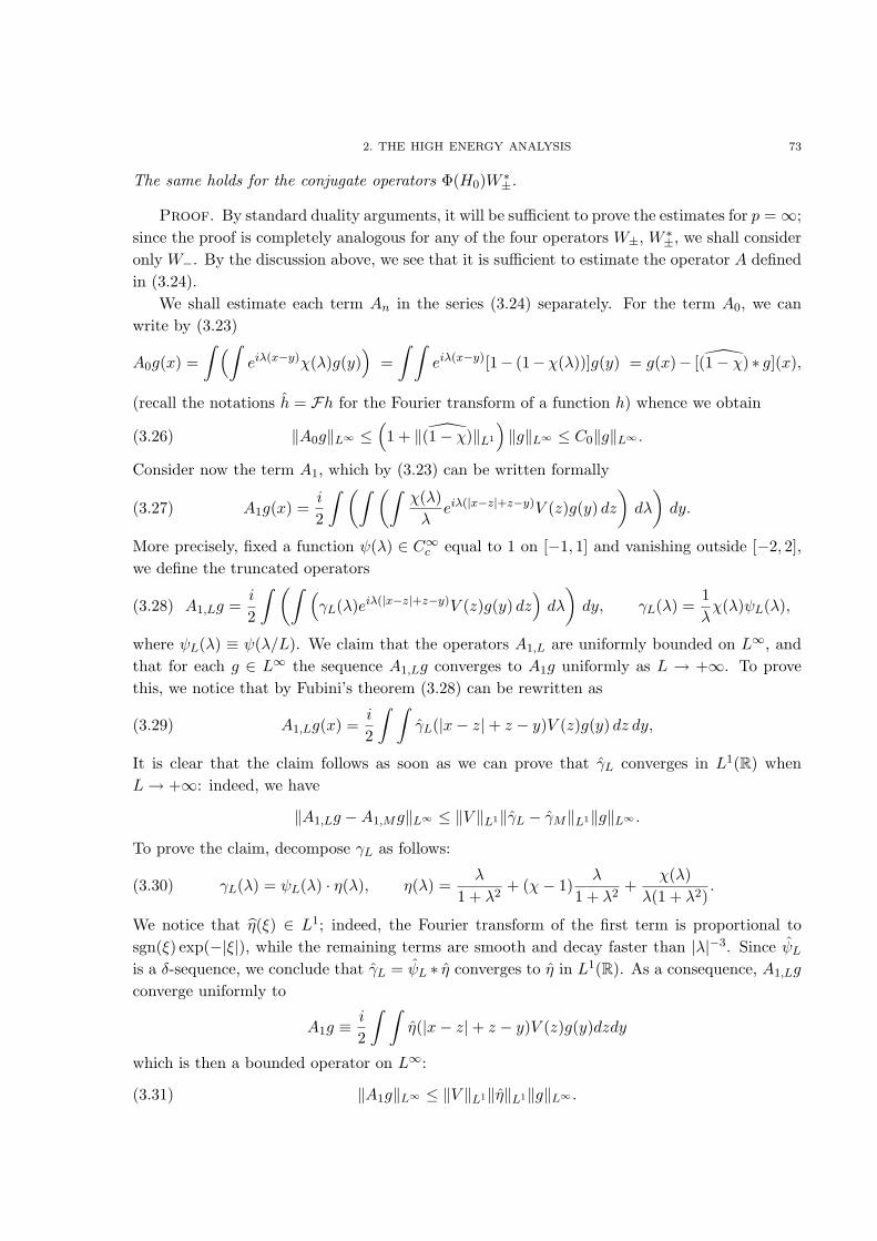
2. THE HIGH ENERGY ANALYSIS 73
The same holds for the conjugate operators Φ(H0)W ∗±.
Proof. By standard duality arguments, it will be sufficient to prove the estimates for p = ∞;since the proof is completely analogous for any of the four operators W±, W ∗
±, we shall consideronly W−. By the discussion above, we see that it is sufficient to estimate the operator A definedin (3.24).
We shall estimate each term An in the series (3.24) separately. For the term A0, we canwrite by (3.23)
A0g(x) =∫ (∫
eiλ(x−y)χ(λ)g(y))
=∫ ∫
eiλ(x−y)[1− (1−χ(λ))]g(y) = g(x)− [ (1− χ) ∗ g](x),
(recall the notations h = Fh for the Fourier transform of a function h) whence we obtain
(3.26) ‖A0g‖L∞ ≤(1 + ‖ (1− χ)‖L1
)‖g‖L∞ ≤ C0‖g‖L∞ .
Consider now the term A1, which by (3.23) can be written formally
(3.27) A1g(x) =i
2
∫ (∫ (∫χ(λ)λ
eiλ(|x−z|+z−y)V (z)g(y) dz)dλ
)dy.
More precisely, fixed a function ψ(λ) ∈ C∞c equal to 1 on [−1, 1] and vanishing outside [−2, 2],we define the truncated operators
(3.28) A1,Lg =i
2
∫ (∫ (γL(λ)eiλ(|x−z|+z−y)V (z)g(y) dz
)dλ
)dy, γL(λ) =
1λχ(λ)ψL(λ),
where ψL(λ) ≡ ψ(λ/L). We claim that the operators A1,L are uniformly bounded on L∞, andthat for each g ∈ L∞ the sequence A1,Lg converges to A1g uniformly as L → +∞. To provethis, we notice that by Fubini’s theorem (3.28) can be rewritten as
(3.29) A1,Lg(x) =i
2
∫ ∫γL(|x− z|+ z − y)V (z)g(y) dz dy,
It is clear that the claim follows as soon as we can prove that γL converges in L1(R) whenL→ +∞: indeed, we have
‖A1,Lg −A1,Mg‖L∞ ≤ ‖V ‖L1‖γL − γM‖L1‖g‖L∞ .
To prove the claim, decompose γL as follows:
(3.30) γL(λ) = ψL(λ) · η(λ), η(λ) =λ
1 + λ2+ (χ− 1)
λ
1 + λ2+
χ(λ)λ(1 + λ2)
.
We notice that η(ξ) ∈ L1; indeed, the Fourier transform of the first term is proportional tosgn(ξ) exp(−|ξ|), while the remaining terms are smooth and decay faster than |λ|−3. Since ψL
is a δ-sequence, we conclude that γL = ψL ∗ η converges to η in L1(R). As a consequence, A1,Lg
converge uniformly to
A1g ≡i
2
∫ ∫η(|x− z|+ z − y)V (z)g(y)dzdy
which is then a bounded operator on L∞:
(3.31) ‖A1g‖L∞ ≤ ‖V ‖L1‖η‖L1‖g‖L∞ .

74 3. DISPERSION VIA WAVE OPERATORS
To conclude the proof, it remains to estimate the operators An for n ≥ 2. By the explicitformula (3.22) we obtain
Ang(x) =in
2n
∫ψn(λ)eiλ(|x−y1|+|y1−y2|+···+|yn−1−yn|+yn−y)
n∏j=1
V (yj)g(y) dy1 . . . dyn dλ dy,
where ψn(λ) := χ(λ)/λn. By Fubini’s Theorem this can be written
Ang(x) =in
2n
∫ψn(|x− y1|+ |y1 − y2|+ · · ·+ |yn−1 − yn|+ yn − y)
n∏j=1
V (yj)g(y) dy1 . . . dyn dy,
and then we immediately get the inequality
(3.32) ‖Ang(x)‖L∞ ≤ 12n‖V ‖n
L1‖ψn‖L1‖g‖L∞ .
To compute the norm of ψn, introduce the scaling operators Sh defined as Shg(x) = g(hx); thenwe can write
ψn(λ) = λ−n0 · S1/λ0
(χ0(λ)λn
)where χ0(λ) := χ(λ · λ0), λ0 = ‖V ‖L1 .
and hence
‖ψn‖L1 = λ−n0 ‖F (χ0/λ
n) ‖L1 ≤ Cλ−n0 ‖〈ξ〉2F (χ0/λ
n) ‖L∞
≤ Cλ−n0 ‖(1−∆) (χ0/λ
n) ‖L1 ≤ C0n2λ−n
0 ≡ C0n2‖V ‖−n
L1
for some constant C0 independent of n and λ0 This inequality together with (3.32) gives
(3.33) ‖Ang(x)‖L∞ ≤ C0n22−n‖g‖L∞ .
By the estimates (3.26), (3.31), (3.33) and by formula (3.24) we conclude the proof of theLemma. �
3. Fourier properties of the Jost Functions
Throughout this section we shall assume that V ∈ L11(R) (at least).
The Jost functions f±(z, x) are defined as the solutions of −f ′′±(z, x) + V (x)f±(z, x) =z2f±(z, x) satisfying the asymptotic conditions
∣∣f±(z, x)− e±izx∣∣ → 0 as x → ±∞. It is well
known (see [36]) that f±(λ, x) are well defined for all λ, x ∈ R. Using the Jost functions itis possible to write the following explicit representation of the integral kernel of the perturbedresolvent RV (λ2 ± i0):
(3.34) K±(x, y) =1
2πif+(±λ, y)f−(±λ, x)
W (±λ)for x < y,
and x and y reversed for x > y; here W (λ) denotes the Wronskian of f+, f− defined in (3.4). Itis always true (see [36]) that W (λ) 6= 0 for any real λ 6= 0; thus the only possible real zero ofthe Wronskian is at λ = 0, and when W (0) = 0 we say that 0 is a resonance for −∆ + V .
The modified Jost functions m± are given by the relation f±(λ, x) = e±iλxm±(λ, x); equiva-lently, they can be characterized as the unique solutions of the equationsm′′
±(λ, x)±2iλm′±(λ, x) =
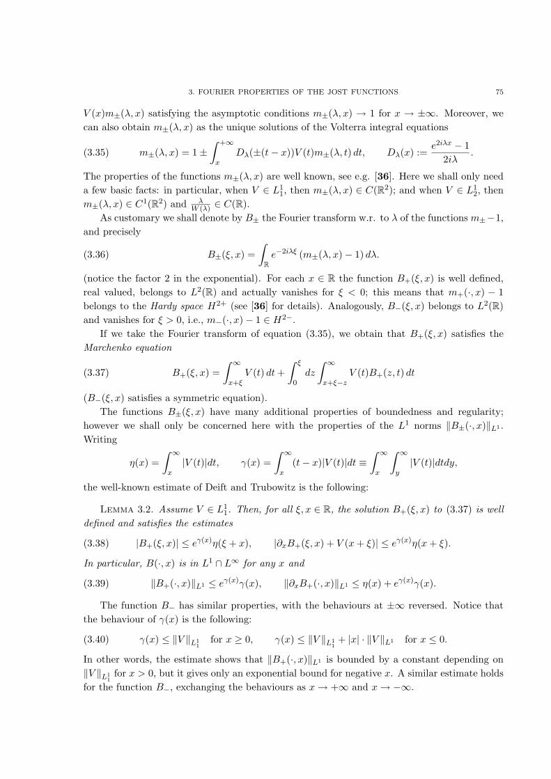
3. FOURIER PROPERTIES OF THE JOST FUNCTIONS 75
V (x)m±(λ, x) satisfying the asymptotic conditions m±(λ, x) → 1 for x → ±∞. Moreover, wecan also obtain m±(λ, x) as the unique solutions of the Volterra integral equations
(3.35) m±(λ, x) = 1±∫ +∞
xDλ(±(t− x))V (t)m±(λ, t) dt, Dλ(x) :=
e2iλx − 12iλ
.
The properties of the functions m±(λ, x) are well known, see e.g. [36]. Here we shall only needa few basic facts: in particular, when V ∈ L1
1, then m±(λ, x) ∈ C(R2); and when V ∈ L12, then
m±(λ, x) ∈ C1(R2) and λW (λ) ∈ C(R).
As customary we shall denote by B± the Fourier transform w.r. to λ of the functions m±−1,and precisely
(3.36) B±(ξ, x) =∫
Re−2iλξ (m±(λ, x)− 1) dλ.
(notice the factor 2 in the exponential). For each x ∈ R the function B+(ξ, x) is well defined,real valued, belongs to L2(R) and actually vanishes for ξ < 0; this means that m+(·, x) − 1belongs to the Hardy space H2+ (see [36] for details). Analogously, B−(ξ, x) belongs to L2(R)and vanishes for ξ > 0, i.e., m−(·, x)− 1 ∈ H2−.
If we take the Fourier transform of equation (3.35), we obtain that B+(ξ, x) satisfies theMarchenko equation
(3.37) B+(ξ, x) =∫ ∞
x+ξV (t) dt+
∫ ξ
0dz
∫ ∞
x+ξ−zV (t)B+(z, t) dt
(B−(ξ, x) satisfies a symmetric equation).The functions B±(ξ, x) have many additional properties of boundedness and regularity;
however we shall only be concerned here with the properties of the L1 norms ‖B±(·, x)‖L1 .Writing
η(x) =∫ ∞
x|V (t)|dt, γ(x) =
∫ ∞
x(t− x)|V (t)|dt ≡
∫ ∞
x
∫ ∞
y|V (t)|dtdy,
the well-known estimate of Deift and Trubowitz is the following:
Lemma 3.2. Assume V ∈ L11. Then, for all ξ, x ∈ R, the solution B+(ξ, x) to (3.37) is well
defined and satisfies the estimates
(3.38) |B+(ξ, x)| ≤ eγ(x)η(ξ + x), |∂xB+(ξ, x) + V (x+ ξ)| ≤ eγ(x)η(x+ ξ).
In particular, B(·, x) is in L1 ∩ L∞ for any x and
(3.39) ‖B+(·, x)‖L1 ≤ eγ(x)γ(x), ‖∂xB+(·, x)‖L1 ≤ η(x) + eγ(x)γ(x).
The function B− has similar properties, with the behaviours at ±∞ reversed. Notice thatthe behaviour of γ(x) is the following:
(3.40) γ(x) ≤ ‖V ‖L11
for x ≥ 0, γ(x) ≤ ‖V ‖L11+ |x| · ‖V ‖L1 for x ≤ 0.
In other words, the estimate shows that ‖B+(·, x)‖L1 is bounded by a constant depending on‖V ‖L1
1for x > 0, but it gives only an exponential bound for negative x. A similar estimate holds
for the function B−, exchanging the behaviours as x→ +∞ and x→ −∞.

76 3. DISPERSION VIA WAVE OPERATORS
A crucial tool in the study of the low energy case will be an essential improvement of the(3.39): indeed, we can prove that the norm of B+ (resp. B−) has at most a linear growth asx→ −∞ (resp. x→ +∞).
Lemma 3.3. Assume V ∈ L11; then the functions B±(ξ, x) satisfy the estimates
(3.41) ‖B±(·, x)‖L1 ≤ C for ±x ≥ 0, ‖B±(·, x)‖L1 ≤ C〈x〉 for ±x ≤ 0
for some constant C depending on ‖V ‖L11.
Proof. We prove the result for B+, the proof for B− is identical. The behaviour for positivex is already contained in the Deift-Trubowitz estimate. Now, starting from the Marchenkoequation (3.37), we integrate with respect to ξ from 0 to ∞ (recall that B± vanish for ξ < 0)and we have immediately
‖B+(·, x)‖L1 ≤√
2〈x〉 · ‖V ‖L11+∫ ∞
0dξ
∫ ξ
−∞dz
∫ ∞
x+ξ−z|V (t)| · |B+(z, t)| dt.
Setting z′ := ξ − z and exchanging the order of integration we obtain
(3.42) ‖B+(·, x)‖L1 ≤√
2〈x〉 · ‖V ‖L11+∫ ∞
x|V (t)| · (t− x) · ‖B+(·, t)‖L1 dt.
Now we remark that∫ ∞
xt|V (t)| · ‖B+(·, t)‖L1dt ≤
∫ ∞
0t|V (t)| · ‖B+(·, t)‖L1dt
which is obvious when x > 0 and is also evident for x < 0 since the integral from x to 0 isnegative. Using the Deift-Trubowitz estimate (3.39) we see that ‖B+(·, t)‖ ≤ C0 = C0(‖V ‖L1
1)
for t > 0, and hence in conclusion∫ ∞
xt|V (t)| · ‖B+(·, t)‖L1dt ≤ C1 ≡ C1(‖V ‖L1
1) for all x ∈ R.
Thus inequality (3.42) gives
‖B+(·, x)‖L1 ≤√
2〈x〉 · ‖V ‖L11+ C1(‖V ‖L1
1) + |x|
∫ ∞
x|V (t)| · ‖B+(·, t)‖L1dt
which implies
(3.43)1〈x〉
‖B+(·, x)‖L1 ≤ C2(‖V ‖L11) +
∫ ∞
x〈t〉|V (t)|‖B+(·, t)‖L1
〈t〉dt.
Applying Gronwall’s lemma for x < 0 we conclude the proof. �
In the resonant case W (0) = 0 it will be necessary to make the stronger assumption V ∈ L12.
In this case, we know that the Jost functions are C1 in both variables and we shall study thebehaviour of the functions
(3.44) C±(ξ, x) =∫
Re−2iλξ∂λm±(λ, x)dξ ≡ 2iξB±(ξ, x).
As above, a direct application of the Deift-Trubowitz estimate gives an optimal bound only ona half line. Indeed, if we multiply (3.38) by 2ξ and integrate in ξ we obtain
(3.45) ‖C+(·, x)‖L1 ≤ 2eγ(x)
∫ ∞
0ξ
∫ ∞
x+ξ|V (t)|dtdξ = eγ(x)
∫ ∞
x(t− x)2|V (t)|dt

3. FOURIER PROPERTIES OF THE JOST FUNCTIONS 77
after exchanging the order of integration. Recalling (3.40) we obtain that ‖C+(·, x)‖L1 ≤C(‖V ‖L1
2) for x ≥ 0, but we can only get an exponential growth for negative x (symmetric
result for C−).We can improve this estimate by a different argument:
Lemma 3.4. Assume V ∈ L12; then the functions C±(ξ, x) = 2iξB±(ξ, x) satisfy
(3.46) ‖C±(·, x)‖L1 ≤ C for ±x ≥ 0, ‖C±(·, x)‖L1 ≤ C〈x〉2 for ±x ≤ 0
for some constant C depending on ‖V ‖L12.
Proof. We will consider only C+; the proof for C− is identical. We have already provedabove the estimate of C+ on the positive half-line. To prove the estimate for x < 0 we startagain from Marchenko’s equation (3.37); if we multiply both sides by 2ξ and integrate in ξ weobtain
‖C+(·, x)‖L1 ≤ 2∫ ∞
0
∫ ∞
x+ξ|V (t)| · ξ dtdξ + 2
∫ ∞
0dξ
∫ ξ
0dσ
∫ ∞
x+ξ−σ|V (t)| · |B+(σ, t)| · ξ dt
≡ 2∫ ∞
x(t− x)2|V |dt+
∫ ∞
x|V |(t− x)2‖B+(·, t)‖L1dt+
∫ ∞
x|V |(t− x)‖C+(·, t)‖L1dt(3.47)
after a suitable rearrangement of the order of integration. Call the three integrals on the rightI, II, III respectively. For the first one we have obviously I ≤ 4〈x〉2‖V ‖L1
2. For the second one,
we remark that (t− x)2 ≤ x2 when x < t < 0, while (t− x)2 ≤ 2t2 + 2x2 when t > 0, so that
II ≤ x2
∫ 0
x|V (t)| · ‖B(·, t)‖L1dt+ 2
∫ ∞
0(t2 + x2)|V (t)| · ‖B(·, t)‖L1dt;
recalling (3.41), this implies
(3.48) II ≤ x2
∫ 0
x|V (t)|〈t〉dt · C(‖V ‖L1
1) + 2
∫ ∞
0(t2 + x2)|V (t)| · C(‖V ‖L1
1) ≤ 〈x〉2C(‖V ‖L1
2).
For the last term we proceed as follows: we write
III =∫ ∞
xt|V (t)|‖C+(·, t)‖L1dt− x
∫ ∞
x|V (t)|‖C+(·, t)‖L1dt
and, as above, we remark that the first integral increases if we replace the lower integration limitwith 0: ∫ ∞
xt|V (t)|‖C+(·, t)‖L1dt ≤
∫ ∞
0t|V (t)|‖C+(·, t)‖L1dt ≤ C(‖V ‖L1
2)
where we have used the bound for x > 0 already proved. Thus we have
(3.49) III ≤ C(‖V ‖L12) + 〈x〉
∫ ∞
x〈t〉2|V (t)| · 〈t〉−2‖C+(·, t)‖L1dt.
In conclusion we have proved that
(3.50) 〈x〉−2‖C+(·, x)‖L1 ≤ C(‖V ‖L12) +
∫ ∞
x〈t〉2|V (t)| · 〈t〉−2‖C+(·, t)‖L1dt.
Applying as before Gronwall’s lemma for x < 0, we conclude the proof of the Lemma. �

78 3. DISPERSION VIA WAVE OPERATORS
A useful consequence of (3.46) is an estimate of the Fourier transform of the functions
(3.51) n±(λ, x) =m±(λ, x)−m±(0, x)
λ
which are clearly related to the derivatives ∂λm±; the usefulness of these quantities in theresonant case had already been remarked in [5].
Corollary 3.1. Assume V ∈ L12; then the functions C±(ξ, x) =
∫R e
−2iλξn±(λ, x)dλ satisfy
(3.52) ‖C±(·, x)‖L1 ≤ C for ±x ≥ 0, ‖C±(·, x)‖L1 ≤ C〈x〉2 for ±x ≤ 0
for some constant C depending on ‖V ‖L12.
Proof. Since n±(λ, x) =∫ 10 ∂λm±(λs, x)ds, we can write, using Fubini’s theorem and the
rescaling properties of the Fourier transform,
C±(ξ, x) =∫ 1
0Fλ→ξ (∂λm±(λs, x)) ds =
∫ 1
0s−1C±(ξ/s, x)ds.
The integral Minkowski inequality now gives
‖C±(·, x)‖L1 ≤∫ 1
0s−1‖C±(·/s, x)‖L1ds ≡
∫ 1
0‖C±(·, x)‖L1ds ≡ ‖C±(·, x)‖L1
and by (3.46) the proof is concluded. �
We conclude this section by studying the Fourier properties of the Wronskian W (λ) definedin (3.4), which can be equivalently written
W (λ) = m+(λ, 0)∂xm−(λ, 0)− ∂xm+(λ, 0)m−(λ, 0)− 2iλm+(λ, 0)m−(λ, 0).
Notice that the following result is also proved in [49] by partly different arguments.
Lemma 3.5. Let χ(λ) ∈ C∞0 (R) be a smooth cutoff. If V ∈ L11(R) and W (0) 6= 0 then
(3.53) F(χ(λ)W (λ)
)∈ L1(R).
On the other hand, if V ∈ L12(R) and W (0) = 0 then
(3.54) F(χ(λ)λW (λ)
)∈ L1(R).
Proof. Let χ1 ∈ C∞0 (R) be a second cutoff such that χ1 ≡ 1 on the support of χ. By theDeift-Trubowitz estimates (see Lemma 3.2) we know that both m±(λ, 0) − 1 and ∂xm±(λ, 0)have Fourier transform in L1; then writing
χ1W (λ) ≡ χ1m+(λ, 0)∂xm−(λ, 0)− χ1∂xm+(λ, 0)m−(λ, 0)− 2iλχ1m+(λ, 0)m−(λ, 0)
we see that χ1W can be written as a sum of products in which each factor has a Fouriertransform in L1, and we conclude that χ1W has Fourier transform in L1.
Recall now that by Wiener’s Lemma, if a function a(λ) does not vanish on the support ofb(λ) and both a, b ∈ L1, we have also F(b/a) ∈ L1. This implies that∥∥∥∥Fλ→ξ
(χ(λ)W (λ)
)∥∥∥∥L1
ξ
≡∥∥∥∥Fλ→ξ
(χ(λ)
χ1(λ)W (λ)
)∥∥∥∥L1
ξ
<∞.
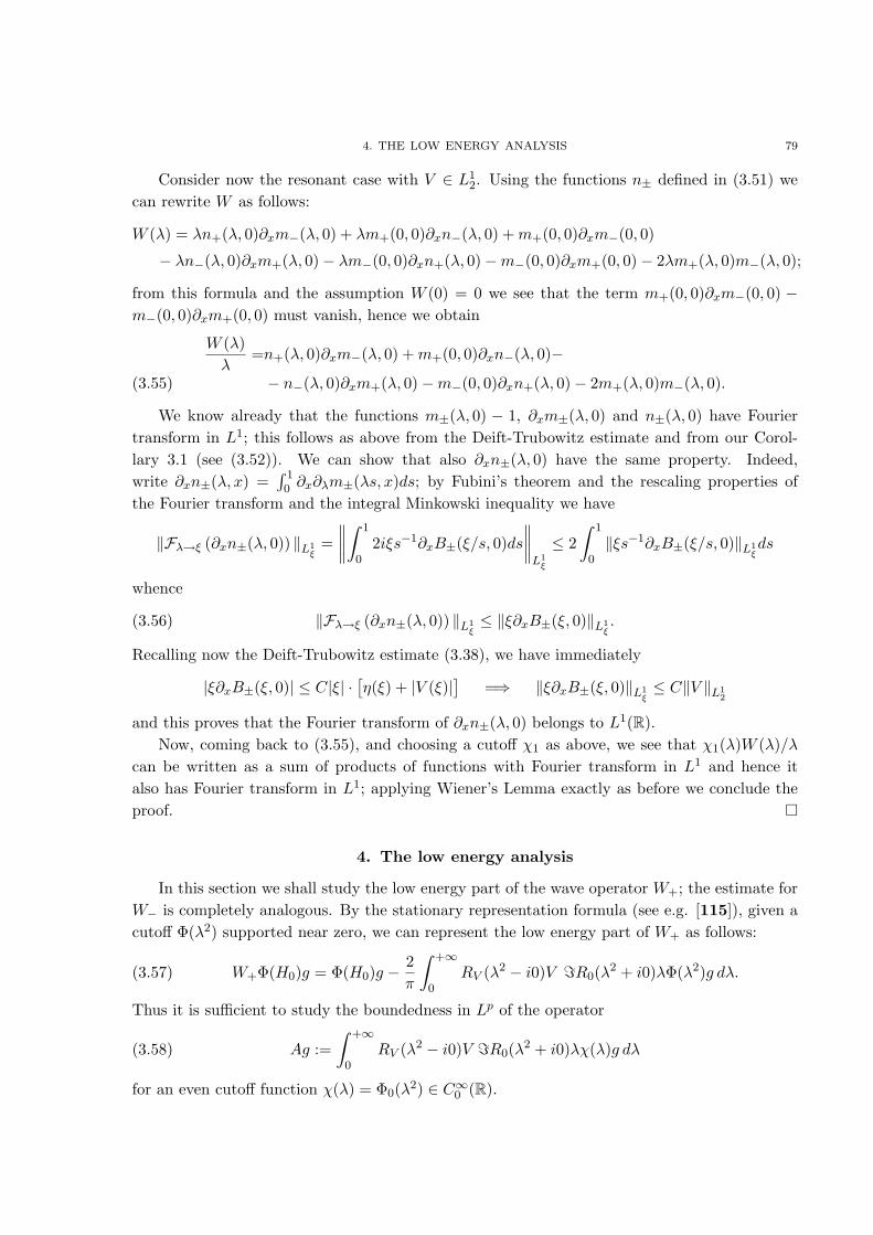
4. THE LOW ENERGY ANALYSIS 79
Consider now the resonant case with V ∈ L12. Using the functions n± defined in (3.51) we
can rewrite W as follows:
W (λ) = λn+(λ, 0)∂xm−(λ, 0) + λm+(0, 0)∂xn−(λ, 0) +m+(0, 0)∂xm−(0, 0)
− λn−(λ, 0)∂xm+(λ, 0)− λm−(0, 0)∂xn+(λ, 0)−m−(0, 0)∂xm+(0, 0)− 2λm+(λ, 0)m−(λ, 0);
from this formula and the assumption W (0) = 0 we see that the term m+(0, 0)∂xm−(0, 0) −m−(0, 0)∂xm+(0, 0) must vanish, hence we obtain
W (λ)λ
=n+(λ, 0)∂xm−(λ, 0) +m+(0, 0)∂xn−(λ, 0)−
− n−(λ, 0)∂xm+(λ, 0)−m−(0, 0)∂xn+(λ, 0)− 2m+(λ, 0)m−(λ, 0).(3.55)
We know already that the functions m±(λ, 0) − 1, ∂xm±(λ, 0) and n±(λ, 0) have Fouriertransform in L1; this follows as above from the Deift-Trubowitz estimate and from our Corol-lary 3.1 (see (3.52)). We can show that also ∂xn±(λ, 0) have the same property. Indeed,write ∂xn±(λ, x) =
∫ 10 ∂x∂λm±(λs, x)ds; by Fubini’s theorem and the rescaling properties of
the Fourier transform and the integral Minkowski inequality we have
‖Fλ→ξ (∂xn±(λ, 0)) ‖L1ξ
=∥∥∥∥∫ 1
02iξs−1∂xB±(ξ/s, 0)ds
∥∥∥∥L1
ξ
≤ 2∫ 1
0‖ξs−1∂xB±(ξ/s, 0)‖L1
ξds
whence
(3.56) ‖Fλ→ξ (∂xn±(λ, 0)) ‖L1ξ≤ ‖ξ∂xB±(ξ, 0)‖L1
ξ.
Recalling now the Deift-Trubowitz estimate (3.38), we have immediately
|ξ∂xB±(ξ, 0)| ≤ C|ξ| ·[η(ξ) + |V (ξ)|
]=⇒ ‖ξ∂xB±(ξ, 0)‖L1
ξ≤ C‖V ‖L1
2
and this proves that the Fourier transform of ∂xn±(λ, 0) belongs to L1(R).Now, coming back to (3.55), and choosing a cutoff χ1 as above, we see that χ1(λ)W (λ)/λ
can be written as a sum of products of functions with Fourier transform in L1 and hence italso has Fourier transform in L1; applying Wiener’s Lemma exactly as before we conclude theproof. �
4. The low energy analysis
In this section we shall study the low energy part of the wave operator W+; the estimate forW− is completely analogous. By the stationary representation formula (see e.g. [115]), given acutoff Φ(λ2) supported near zero, we can represent the low energy part of W+ as follows:
(3.57) W+Φ(H0)g = Φ(H0)g −2π
∫ +∞
0RV (λ2 − i0)V =R0(λ2 + i0)λΦ(λ2)g dλ.
Thus it is sufficient to study the boundedness in Lp of the operator
(3.58) Ag :=∫ +∞
0RV (λ2 − i0)V =R0(λ2 + i0)λχ(λ)g dλ
for an even cutoff function χ(λ) = Φ0(λ2) ∈ C∞0 (R).
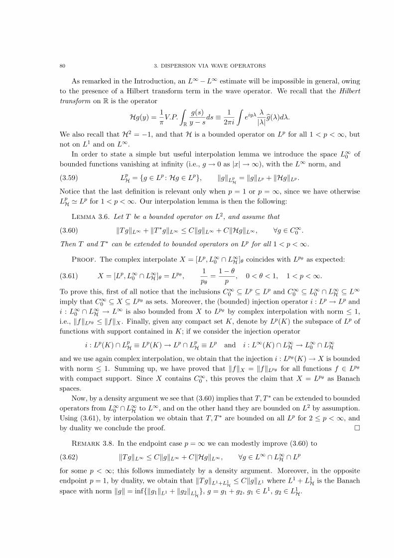
80 3. DISPERSION VIA WAVE OPERATORS
As remarked in the Introduction, an L∞−L∞ estimate will be impossible in general, owingto the presence of a Hilbert transform term in the wave operator. We recall that the Hilberttransform on R is the operator
Hg(y) =1πV.P.
∫R
g(s)y − s
ds ≡ 12πi
∫eiyλ λ
|λ|g(λ)dλ.
We also recall that H2 = −1, and that H is a bounded operator on Lp for all 1 < p < ∞, butnot on L1 and on L∞.
In order to state a simple but useful interpolation lemma we introduce the space L∞0 ofbounded functions vanishing at infinity (i.e., g → 0 as |x| → ∞), with the L∞ norm, and
(3.59) LpH = {g ∈ Lp : Hg ∈ Lp}, ‖g‖Lp
H= ‖g‖Lp + ‖Hg‖Lp .
Notice that the last definition is relevant only when p = 1 or p = ∞, since we have otherwiseLpH ' Lp for 1 < p <∞. Our interpolation lemma is then the following:
Lemma 3.6. Let T be a bounded operator on L2, and assume that
(3.60) ‖Tg‖L∞ + ‖T ∗g‖L∞ ≤ C‖g‖L∞ + C‖Hg‖L∞ , ∀g ∈ C∞0 .
Then T and T ∗ can be extended to bounded operators on Lp for all 1 < p <∞.
Proof. The complex interpolate X = [Lp, L∞0 ∩ L∞H ]θ coincides with Lpθ as expected:
(3.61) X = [Lp, L∞0 ∩ L∞H ]θ = Lpθ ,1pθ
=1− θ
p, 0 < θ < 1, 1 < p <∞.
To prove this, first of all notice that the inclusions C∞0 ⊆ Lp ⊆ Lp and C∞0 ⊆ L∞0 ∩ L∞H ⊆ L∞
imply that C∞0 ⊆ X ⊆ Lpθ as sets. Moreover, the (bounded) injection operator i : Lp → Lp andi : L∞0 ∩ L∞H → L∞ is also bounded from X to Lpθ by complex interpolation with norm ≤ 1,i.e., ‖f‖Lpθ ≤ ‖f‖X . Finally, given any compact set K, denote by Lp(K) the subspace of Lp offunctions with support contained in K; if we consider the injection operator
i : Lp(K) ∩ LpH ≡ Lp(K) → Lp ∩ Lp
H ≡ Lp and i : L∞(K) ∩ L∞H → L∞0 ∩ L∞Hand we use again complex interpolation, we obtain that the injection i : Lpθ(K) → X is boundedwith norm ≤ 1. Summing up, we have proved that ‖f‖X = ‖f‖Lpθ for all functions f ∈ Lpθ
with compact support. Since X contains C∞0 , this proves the claim that X = Lpθ as Banachspaces.
Now, by a density argument we see that (3.60) implies that T, T ∗ can be extended to boundedoperators from L∞0 ∩L∞H to L∞, and on the other hand they are bounded on L2 by assumption.Using (3.61), by interpolation we obtain that T, T ∗ are bounded on all Lp for 2 ≤ p < ∞, andby duality we conclude the proof. �
Remark 3.8. In the endpoint case p = ∞ we can modestly improve (3.60) to
(3.62) ‖Tg‖L∞ ≤ C‖g‖L∞ + C‖Hg‖L∞ , ∀g ∈ L∞ ∩ L∞H ∩ Lp
for some p < ∞; this follows immediately by a density argument. Moreover, in the oppositeendpoint p = 1, by duality, we obtain that ‖Tg‖L1+L1
H≤ C‖g‖L1 where L1 + L1
H is the Banachspace with norm ‖g‖ = inf{‖g1‖L1 + ‖g2‖L1
H}, g = g1 + g2, g1 ∈ L1, g2 ∈ L1
H.

4. THE LOW ENERGY ANALYSIS 81
We are now ready to prove our estimate of the low frequency part of the wave operator:
Lemma 3.7. Assume V ∈ L11 and the nonresonant condition W (0) 6= 0 is satisfied. Let
Φ(λ2) be a smooth compactly supported cutoff function. Then the low energy parts of the waveoperators W± satisfy the estimates
(3.63) ‖W±Φ(H0)g‖L∞ ≤ C (‖g‖L∞ + ‖Hg‖L∞) ∀g ∈ L1 ∩ L∞ ∩ L∞Hand hence can be extended to bounded operatos on Lp, for all 1 < p <∞. The same propertieshold for the conjugate operators Φ(H0)W ∗
±.
Proof. The proof for the operators W± and W ∗± is completely analogous, hence we shall
focus on the estimate for W+. By Lemma 3.6, it is sufficient to prove that W+Φ(H0) satisfies(3.63); moreover, using the stationary representation formula (3.57), the problem is reduced toestimating the operator A defined by (3.58).
By the explicit expression of the kernel of RV in terms of the Jost functions (3.34), we cansplit A as A = A1 +A2 where (forgetting constants)
(3.64) A1g(x) =∫ +∞
0dλ
∫x<y
dyf+(−λ, y)f−(−λ, x)
W (−λ)V (y)λχ(λ)=R0(λ2 + i0)g(y)
while A2 is given by a symmetric formula. In the following we shall estimate the operator A1;the proof for A2 is completely analogous.
By the relations f±(λ, x) = e±iλxm±(λ, x) and
m±(−λ, x) = m±(λ, x), W (−λ) = W (λ)
(see. e.g. [36]), we have
(3.65) A1g(x) =∫ +∞
0dλ
∫x<y
dym+(λ, y)m−(λ, x)
W (λ)V (y)eiλ(x−y)λχ(λ)=R0(λ2 + i0)g(y).
By Fubini’s Theorem we can exchange the order of integration and rewrite (3.65) as follows:(3.66)
A1g(x) =∫
x<yFλ→ξ
(m+(λ, y)m−(λ, x)
W (λ)χ(λ)1(0,+∞)(λ)=R0(λ2 + i0)g(y)
)∣∣∣∣∣ξ=x−y
V (y)dy
where F denotes the standard Fourier transform from the λ to the ξ variable and 1(0,+∞) is thecharacteristic function of the half line (0,+∞).
Now choose a C∞0 cutoff function ψ(λ) such that ψ ≡ 1 on suppχ ; then the function
G(λ, x, y) =m+(λ, y)m−(λ, x)
W (λ)χ(λ)1(0,+∞)(λ)=R0(λ2 + i0)g(y)
can be written as a product
(3.67) G(λ, x, y) = F1(λ, y)F2(λ, x)F3(λ)F4(λ, y)
where
F1(λ, y) = m+(λ, y)ψ(λ), F2(λ, x) = m−(λ, x)ψ(λ), F3(λ) =ψ(λ)W (λ)
andF4(λ, y) = χ(λ)1(0,+∞)(λ)=R0(λ2 + i0)g(y).

82 3. DISPERSION VIA WAVE OPERATORS
We are interested in the Fourier transform of G with respect to λ; this can be written as theconvolution of the transforms Fj , j = 1, 2, 3, 4.
By Lemma 3.5 (see (3.53)) we already know that
(3.68) ‖F3(ξ)‖L1ξ
= C0 <∞.
Consider now F1(ξ, y), which can be written
F1(ξ, y) = F((m+(λ, y)− 1)ψ1 + ψ1) = B+(−ξ/2, y) ∗ ψ1 + ψ1
(the inessential factor 1/2 comes from the nonstandard Fourier transform used in Definition(3.36), and the minus sign from the conjugation). Recalling Lemma 3.3, we get
‖F1(·, y)‖L1 ≤
{C for y ≥ 0C〈y〉 for y ≤ 0
‖F2(·, x)‖L1 ≤
{C for x ≤ 0C〈x〉 for x ≥ 0
for some C depending on ‖V ‖L11. Recalling that in (3.66) we have x < y, we can write
‖F(F1F2)‖L1ξ≤ ‖F1(·, y)‖L1‖F2(·, x)‖L1 ≤
C〈y〉 for x < y < 0C for x < 0 < y
C〈x〉 ≤ C〈y〉 for 0 < x < y
and in conclusion
(3.69) ‖F(F1F2)‖L1ξ≤ C(‖V ‖L1
1) · 〈y〉.
Coming back to G(λ, x, y), if we put together (3.68) and (3.69) and we use Young’s inequality,we have proved that, for x < y,
(3.70) ‖G(·, x, y)‖L∞ ≤ C(‖V ‖L11) · 〈y〉 · ‖F4(·, y)‖L∞ .
It remains to estimate
‖F4(·, y)‖L∞ ≡ supξ
∣∣Fλ→ξ
(χ(λ)1(0,+∞)(λ)λ=R0(λ2 + i0)g(y)
)∣∣ .We have
F(χ(λ)1(0,+∞)(λ)λ=R0(λ2 + i0)g(y)
)=
∫ ∞
0eiλξλχ(λ)=R0(λ2 + i0)g(y)dλ
≡ Ceiξ√
H0χ(√H0)g
by the spectral theorem. Now we remark that the function
U(ξ, y) = eiξ√
H0χ(√H0)g
is a solution of the one dimensional wave equation
Uξξ +H0U ≡ Uξξ − Uyy = 0,
with initial data
U(0, y) = U0(y) = χ(√H0)g, Uξ(0, y) = U1(y) = i
√H0χ(
√H0)g.
By the explicit representation formula of the solution to the wave equation we have then
U(ξ, y) =U0(ξ + y) + U0(ξ − y)
2+
12
∫ ξ+y
ξ−yU1(σ)dσ.

4. THE LOW ENERGY ANALYSIS 83
The first term is easy to bound:
(3.71)∣∣∣∣U0(ξ + y) + U0(ξ − y)
2
∣∣∣∣ ≤ ‖U0‖L∞ = ‖χ(√H0)g‖L∞ ≤ C‖g‖L∞
since χ(√H0) is bounded on L∞ as it is well known. On the other hand, we can write
U1(y) = i√H0χ(
√H0)g(y) =
∫eiλy|λ|χ(λ)g(λ)dλ ≡
∫eiλy(−iλ)χ(λ)
iλ
|λ|g(λ)dλ
and this implies, apart from a constant,
U1(y) =d
dyχ(√H0)Hg =⇒
∫ ξ+y
ξ−yU1(σ)dσ = χ(
√H0)Hg(ξ + y)− χ(
√H0)Hg(ξ − y).
In conclusion ∣∣∣∣12∫ ξ+y
ξ−yU1(σ)dσ
∣∣∣∣ ≤ ‖χ(√H0)Hg‖L∞ ≤ C‖Hg‖L∞
and summing up we have proved that
(3.72) ‖F4‖L∞ξ,y≤ C‖U‖L∞ξ,y
≤ C (‖g‖L∞ + ‖Hg‖L∞) .
By (3.66), (3.70) and (3.72) we finally obtain
‖A1g‖L∞ ≤ C(‖V ‖L11) · (‖g‖L∞ + ‖Hg‖L∞) .
The operator A2 can be estimated in a similar way, and this concludes the proof of the Lemma.�
We pass to the analysis of the resonant case W (0) = 0.
Lemma 3.8. Assume V ∈ L12 and we are in the resonant case W (0) = 0. Let Φ(λ2) be a
smooth compactly supported cutoff function. Then the following estimate holds:
(3.73) ‖W+Φ(H0)g‖L∞ ≤ C (‖g‖L∞ + ‖Hg‖L∞) ∀g ∈ L1 ∩ L∞ ∩ L∞Hwhere H is the Hilbert transform on R, and hence can be extended to bounded operators on Lp,for all 1 < p <∞. The same estimate holds for the conjugate operators Φ(H0)W ∗
±.
Proof. As in the proof of Lemma 3.7, the problem is reduced to estimating the L∞ normof Ag = A1g + A2g where Ajg are defined as above (see (3.65)). The new difficulty now is ofcourse the denominator W (λ) which vanishes at λ = 0. Thus we decompose Ag into severalterms:
Ag = I1 + I2 + II1 + II2 + III1 + III2
where, recalling the notation (3.51).
(3.74) I1 =∫ +∞
0dλ
∫x>y
dy−λ
W (−λ)n+(−λ, y)m−(−λ, x)eiλ(y−x)V (y)λχ(λ)=R0(λ2 + i0)g(y),
(3.75) II1 =∫ +∞
0dλ
∫x>y
dy−λ
W (−λ)m+(0, y)n−(−λ, x)eiλ(y−x)V (y)λχ(λ)=R0(λ2 + i0)g(y),
(3.76) III1 =∫ +∞
0dλ
∫x>y
dym+(0, y)m−(0, x)
W (−λ)V (y)eiλ(y−x)λχ(λ)=R0(λ2 + i0)g(y).
84 3. DISPERSION VIA WAVE OPERATORS
while as usual, I2, II2 and III2 have symmetric expressions with x and y interchanged. Wenotice the expression for III2 which will be necessary in the following:
(3.77) III2 =∫ +∞
0dλ
∫x<y
dym+(0, x)m−(0, y)
W (−λ)V (y)eiλ(x−y)λχ(λ)=R0(λ2 + i0)g(y)
Since W (0) = 0, we know that for λ = 0 the Jost functions f+(0, x) ≡ m+(0, x) andf−(0, x) ≡ m−(0, x) are linearly dependent, i.e.,
(3.78) m−(0, x) = c0 ·m+(0, x)
for some constant c0 6= 0. Moreover, by definition m±(0, x) → 1 as ±x→∞, and together with(3.78) this implies that m±(0, x) are bounded on R:
(3.79) |m±(0, x)| ≤ c1, x ∈ R.
Finally, when W (0) = 0 we have (see e.g. [5])
(3.80)∫ +∞
−∞V (y)m±(0, y)dy = 0.
The terms of type I and II are handled in a way very similar to the proof of Lemma 3.7.In order to estimate the term I1, we write it as
I1 =∫
x<yFλ→ξ (G(λ, x, y))|ξ=y−x V (y)dy, G(λ, x, y) = F1(λ, y)F2(λ, x)F3(λ)F4(λ, y),
where, choosing a C∞0 (R) cutoff function ψ such that ψ ≡ 1 on suppχ,
F1(λ, y) = n+(−λ, y), F2(λ, x) = m−(−λ, x)ψ(λ), F3(λ) =ψ(λ)λW (−λ)
and
F4(λ, y) = λχ(λ)1(0,+∞)(λ)=R0(λ2 + i0)g(y).
Then we have
supx<y
‖G(·, x, y)‖L∞ ≤ supx<y
(‖F1(·, y)‖L1 · ‖F2(·, x)‖L1 · ‖F3‖L1 · ‖F4(·, y)‖L∞
)Using Lemma 3.5 we see that ‖F3‖L1 = C0 <∞, and by Lemma 3.2 and Corollary 3.1 we obtainas before (by considering the three cases x < y < 0, x < 0 < y and 0 < x < y)
‖F1(·, y)‖L1 · ‖F2(·, x)‖L1 ≤ C(‖V ‖L12) · 〈y〉2 for x < y.
Thus we arrive at
‖G(·, x, y)‖L∞ ≤ C(‖V ‖L12) · 〈y〉2 · ‖F4(·, y)‖L∞
and the remaining term ‖F4(·, y)‖L∞ has already been estimated in (3.72). Summing up wehave proved that
|I1| ≤ C(‖V ‖L12) · (‖g‖L∞ + ‖Hg‖L∞) .
The estimate of I2 is completely analogous; the estimate of the terms II1 and II2 is even easier,keeping into account that the functions m±(0, x) are bounded on R (see (3.79)).
4. THE LOW ENERGY ANALYSIS 85
Consider now the more delicate terms III1, III2. Since m−(0, x) = c0 ·m+(0, x) we can putthe two integrals back together as follows:
III1 + III2 = c0
∫ +∞
0dλ
∫dym+(0, y)m+(0, x)
W (−λ)V (y)eiλ|y−x|λχ(λ)=R0(λ2 + i0)g(y).
We decompose this integral in a different way:
III1 + III2 = c0IV1 + c0IV2
where
(3.81) IV1 =∫ +∞
0dλ
∫dym+(0, y)m+(0, x)
W (−λ)V (y)
[eiλ|y−x| − eiλ|x|
]λχ(λ)=R0(λ2 + i0)g(y)
and
(3.82) IV2 =∫ +∞
0dλ
∫dym+(0, y)m+(0, x)
W (−λ)V (y)eiλ|x|λχ(λ)=R0(λ2 + i0)g(y).
Using the identity
eiλ|y−x| − eiλ|x| =∫ 1
0eiλ(s|x−y|+(1−s)|x|)ds · iλ · (|x− y| − |x|)
and Fubini’s theorem we can rewrite IV1 as follows:
IV1 =∫ 1
0ds
∫Fλ→ξ
(λ
W (−λ)λχ(λ)1(0,+∞)(λ)=R0(λ2 + i0)g(y)
)∣∣∣∣ξ=s|x−y|+(1−s)|x|
K dy
whereK = K(x, y) = im+(0, y)m+(0, x)V (y) (|x− y| − |x|) ;
notice that
(3.83) |K(x, y)| ≤ C|y| · |V (y)|
by (3.79). At this point, we can proceed as above using Lemma 3.5 and (3.72) to obtain∥∥∥∥Fλ→ξ
(λ
W (−λ)λχ(λ)1(0,+∞)(λ)=R0(λ2 + i0)g(y)
)∥∥∥∥L∞ξ
≤ C(‖V ‖L12) · (‖g‖L∞ + ‖Hg‖L∞) .
whence the estimate of IV1 follows immediately.To conclude the proof, it remains to estimate the term IV2. By property (3.80) we have
trivially
(3.84)∫ +∞
0dλ
∫dym+(0, y)m+(0, x)
W (−λ)V (y)eiλ|x|λχ(λ)=R0(λ2 + i0)g(0) ≡ 0
(indeed, in the inner integral only V (y) and m+(0, y) depend on y). Thus we can subtract (3.84)from IV2 and rewrite it in the form
IV2 =∫ +∞
0dλ
∫dym+(0, y)m+(0, x)
W (−λ)V (y)eiλ|x|λχ(λ)
[=R0(λ2 + i0)g(y)−=R0(λ2 + i0)g(0)
].
We now use the elementary identity
=R0(λ2 + i0)g(y)−=R0(λ2 + i0)g(0) =∫ y
0∂s
(=R0(λ2 + i0)g(s)
)ds

86 3. DISPERSION VIA WAVE OPERATORS
and we obtain, after applying Fubini’s theorem,
(3.85) IV2 =∫dy
∫ y
0dsm+(0, y)m+(0, x)V (y)
∫ +∞
0eiλ|x|
λχ(λ)W (−λ)
∂s
(=R0(λ2 + i0)g(s)
)dλ
Since
=R0(λ2 + i0)g(x) = − 14λ
∫ ∞
−∞(eiλ(x−y) + e−iλ(x−y))g(y)dy = − 1
4λ(eiλxg(λ) + e−iλxg(−λ))
we can write for λ > 0
∂x=R0(λ2 + i0)g(x) = − i
4λ· λ ·
(λ
|λ|eiλxg(λ) +
−λ| − λ|
e−iλxg(−λ))
and comparing the two identities and recalling the characterization of the Hilbert transform asa Fourier multiplier, we arrive at the formula
∂x=R0(λ2 + i0)g(x) = Cλ=R0(λ2 + i0)Hg(x)
for a suitable constant C. Thus, by (3.85), we obtain (apart from a constant)
IV2 =∫dy
∫ y
0dsm+(0, y)m+(0, x)V (y)
∫ +∞
0eiλ|x|
λ
W (−λ)λχ(λ)=R0(λ2 + i0)Hg(s)dλ
and this can be estimated exactly as the other terms considered above.The proof is concluded. �
CHAPTER 4
Nonlinear Schrodinger equations
The final chapter of this thesis is devoted to some nonlinear applications of the dispersive-type estimates we introduced in the previous part of the work. A lot of physical models areusually described by nonlinear equations, and the first natural mathematical questions for theseequations are related to existence and unicity of the solutions. Here we give two examples ofnonlinear Schrodinger equations, and point out the attention on existence, unicity and blow-upof the solutions. The reference for the details of this chapter are [38] and [40].
1. NLS with time dependent coefficients
The interest for nonlinear Schrodinger equations finds motivations in the great number ofphysical models they describe. Here we consider the following problem:
(4.1){iut(t, x) + a(t)∆u(t, x) = ±|u|γ−1u(t, x)u(0, x) = f(x),
where u : R × Rn → C, f : Rn → C, n ≥ 2, γ ≥ 1 and a(t) ≥ 0 is a real valued function. Inanalogy with the case a(t) ≡ 1, we frequently refer to defocusing equation when we take thepositive sign at the right hand side of (4.1), otherwise we speak of focusing equation.
It is well known that the Cauchy problem (4.1), in the case a(t) = 1, is well posed in L2 forγ < 1+ 4
n and in H1 for γ < 1+ 4n−2 ; in the critical cases, global well-posedness holds, provided
the initial data are small enough, while blow up phenomena can occur for the focusing equationwhen the initial datum is not assumed to be small (see [20], [46], [63]). If a(t) > 0 is strictlypositive, the same techniques used for the constant case a(t) = 1 permit to obtain the sameclassical results.
On the other hand, the literature for the case in which a(t) ≥ 0 can vanish is very small; thiscase can be regarded as a model for a nonrelativistic particle with variable speed of propagation(or equivalently with variable mass), and we are interested in the treatment of the case in whichthe speed can vanish (or equivalently the mass can explode). The motivation for our approach tothis kind of problem is strictly mathematical: the question is how the degeneration of operatora(t)∆ can influence the critical exponents γ for the well-posedness of the Cauchy problem (4.1).
The analogous situation for the semilinear wave equation was treated in [28] first, andfollowed in [29], [34], [39], [72]: the main step is to reduce the problem to a wave equation witha time-dependent potential of order zero, with a suitable change in the time variable, and thenfind suitable a priori energy estimates for the solution. The algebraic structure of Schrodingerequation permits to regard equation (4.1) as a standard nonlinear Schrodinger equation, asit is shown in Section 3; this gives the possibility to use the linear technology for the freeSchrodinger equation (namely Strichartz estimates), with some refinement, and it represents a
87

88 4. NONLINEAR SCHRODINGER EQUATIONS
strong difference with the case of the wave equation, in which the resulting potential does notallow to use classical linear estimates, because it is too singular.
In what follows, the coefficient a will satisfy the following assumptions:
(4.2) a ∈ C(R), a ≥ 0;
(4.3) a vanish on a discrete set Z = {tn}n=0,1,,... ⊂ R with maximum order λ > 0;
(4.4) ∃ε > 0 : a′(t) < 0, if ti − ε < t < ti, and a′(t) > 0, if ti < t < ti + ε, i ∈ N.
The small ε in (4.4) is uniform with respect to i; assumption (4.4) avoids the possibility that acould reach the zeroes with infinite oscillations. Moreover observe that the primitive function
(4.5) A(t) =∫ t
0a(s) ds
is well defined at each t ∈ R.The simplest example is given by
(4.6) a(t) = |t− t0|λ
with λ > 0.The natural questions of well-posedness of the Cauchy problem (4.1) in L2
x and H1x are solved
in the main theorems of this paper. The sketch of the proofs is standard: a contraction argumentbased on Strichartz-type estimates permits to prove local (in time) well-posedness in the naturalspaces, then the continuation to global solution is performed by means on the conservation lawsof equation (4.1), that are investigated in Section 4. The lack of energy conservation for thisequation (see Section 4) represent a strong difference with the case a(t) ≡ 1 and hence the proofof global well-posedness in C(R;H1) requires a more direct investigation on the lifespan of thelocal solutions (see Section 7).
In the special case when a is given by (4.6), the equation is invariant under the followingscaling
(4.7) vε(t, x) = εαu(εβt, εx),
with
(4.8) α =2
(λ+ 1)(γ − 1), β =
2λ+ 1
.
The mass is conserved by this scaling if
(4.9) γ = 1 +4
n(λ+ 1),
while the H1x-norm is conserved for
(4.10) γ = 1 +4
(n− 2)(λ+ 1).
This suggests that (4.9) and (4.10) should be the critical powers for the L2 and H1 well-posedness, respectively, and we can state our main results:
1. NLS WITH TIME DEPENDENT COEFFICIENTS 89
Theorem 4.1. Let n ≥ 2, a satisfy assumptions (4.2), (4.3), (4.4) and let λ > 0 be thehighest order of the zeroes of a. Assume that
1 ≤ γ < 1 +4
n(λ+ 1);
then, for each initial datum f ∈ L2 there exists a unique global solution u ∈ C(R;L2) of theCauchy problem (4.1).
In the critical caseγ = 1 +
4n(λ+ 1)
,
we have global well-posedness in C(R;L2), provided ‖f‖L2 < ε0, for some ε0 > 0 sufficientlysmall.
In the following Theorem we state the local H1 well-posedness for equation (4.1):
Theorem 4.2. Let n ≥ 2, a satisfy assumptions (4.2), (4.3), (4.4) and let λ > 0 be thehighest order of the zeroes of a. Assume that
1 ≤ γ < 1 +4
(n− 2)(λ+ 1);
then, for each initial datum f ∈ H1 there exists a unique local solution u ∈ C(I;H1) of theCauchy problem (4.1), where I is the greatest interval including the origin in which a does notvanish. In the critical case
γ = 1 +4
(n− 2)(λ+ 1)we have local well-posedness in C(I;H1), provided ‖f‖H1 < ε0, for some ε0 > 0 sufficientlysmall.
Remark 4.1. The result of previous theorem includes also the case in which a(0) = 0; inthat case the interval I contains the origin and does not contain any other zero point for thefuncion a. We also remark that the subcritical result in Theorem 4.2 is already known (see forexample Lemma 3.1 in [21]).
We conclude with the following global theorem (valid only in the sub-critical range):
Theorem 4.3. Let n ≥ 3 and let a satisfy assumptions (4.2), (4.3), (4.4) and let λ > 0 bethe highest order of the zeroes of a. Assume that
(4.11) 1 ≤ γ < 1 +4
(n− 2)(λ+ 1);
then, for each initial datum f ∈ H1 there exists a unique global solution u ∈ C(R;H1) of thedefocusing Cauchy problem (4.1).
In the case n = 2, the same result holds, under the more restrictive assumption
(4.12) 1 ≤ γ ≤ 1 +2(λ+ 1)
λ.
Let n ≥ 3 and let us impose the above assumptions, with the more restrictive condition
(4.13) 1 ≤ γ < 1 + min{
4(n− 2)(λ+ 1)
, 1 +4n
};

90 4. NONLINEAR SCHRODINGER EQUATIONS
then, for each initial datum f ∈ H1 there exists a unique global solution u ∈ C(R;H1) of thefocusing Cauchy problem (4.1).
In the case n = 2, the same result holds, under the more restrictive assumption
(4.14) 1 ≤ γ < min{
1 +2(λ+ 1)
λ, 1 +
4n
}.
Remark 4.2. Observe that Theorems 4.1 and 4.3 (that are in fact valid also for λ = 0) coverthe known results for a ≡ 1, also in the case n = 2 (in fact the critical exponent there is ∞).
The crucial role in the contraction argument for the local well-posedness is played byStrichartz estimates. We recall here some well known facts, starting with the following Def-inition:
Definition 4.1. Let n ≥ 2; a couple (p, q) is said to be Schrodinger admissible if thefollowing conditions are satisfied:
(4.15)2p
=n
2− n
q,
(4.16) p > 2 if n = 2, p ≥ 2 if n ≥ 3.
The Schrodinger propagator eit∆ is unitary on L2(Rn) and satisfies the following Strichartzestimates
(4.17) ‖eit∆f‖Lp(I;Lq) ≤ C‖f‖L2 ,
(4.18)∥∥∥∥∫ t
0ei(t−s)∆F (s, ·) ds
∥∥∥∥Lp(I;Lq)
≤ C‖F‖Lep′ (I;Leq′ ),
for all Schrodinger admissible couples (p, q), (p, q), with p′ and q′ the Holder conjugates (see[47], [66]).
In order to use a contraction argument, we need some refinement of estimates (4.17) and(4.18). In the last years, several papers (see e.g. [3], [79]) treated the question of extendingStrichartz estimates to the more general setting of Lorentz spaces Lp,r, that are usually alsodefined by real interpolation of Lp spaces (see [10]). In particular, it has been recently provedin [3] that, for any admissible pair (p, q), (p, q) and r with 2 < r ≤ p, we have
(4.19)∥∥∥∥∫ t
0ei(t−s)∆F (s)ds
∥∥∥∥Lp,r(I;Lq)
≤ C‖F‖Lep′,2(I;Leq′ )∩L2(I;L
2nn+2 ,2
).
The advantage of this estimate is that it reaches the endpoint, but the space Lep′,2(I;Leq′) ∩L2(I;L
2nn+2
,2) is too ”small” to be mapped in a generally bigger space and perform a contraction.Hence we need to prove directly a slightly different family of estimates, as stated in the followingTheorem:
Theorem 4.4. For any Schrodinger admissible pair (p, q), (p, q), with 2 < p, p <∞, and r, ssatisfying
(4.20) p′ ≤ s′ < r ≤ p, r ≥ 2

2. STRICHARTZ ESTIMATES 91
the following estimates hold:
(4.21) ‖eit∆f‖Lp,r(I;Lq,r) ≤ C‖f‖L2 ,
(4.22)∥∥∥∥∫ t
0ei(t−s)∆F (s, ·) ds
∥∥∥∥Lp,r(I;Lq,r)
≤ C‖F‖Lep′,s′ (I;Leq′,s′ ).
Remark 4.3. We find that estimates (4.21) and (4.22) are of independent interest. Theyinvolve Lorentz spaces, both t and x variables, and the nontrivial fact is that these spaces arenot characterized as real interpolation of mixed Lp
tLqx spaces, except for some very particular
cases (see for example [10], [26]); our proof is based on direct dispersive methods. Moreover,we remark that the space at the right hand side in (4.22) is bigger than the space at the righthand side in (4.19), hence (4.22) is stronger in this sense. On the other hand, Theorem 4.4 doesnot comprehend the endpoint estimate, that actually is not needed in the proof of the previouswell-posedness theorems.
The rest of the paper is organized as follows: Section 2 is devoted to the proof of Theorem4.4; in Section 3, by algebraic computations, we transform equation (4.1) into a nonlinearSchroedinger equation with constant coefficients for the linear part; in Section 4 we investigateon the conservation laws of equation (4.1), and in the final part (Sections 5, 6 and 7) we proveTheorems 4.1, 4.2 and 4.3.
2. Strichartz estimates
This section is devoted to the proof of the generalized Strichartz estimates in Theorem 4.4.We prove (4.21) and (4.22) by a standard TT ∗ method based on dispersive estimates (see [47]).For simplicity of notations, we denote the Schrodinger group by U(t) = eit∆. Let us start bythe well known decay
(4.23) ‖U(t)f‖Lq ≤ t−n
2+n
q ‖f‖Lq′ ,
for q ≥ 2, and 1/q + 1/q′ = 1. By interpolation of Lq-dispersive estimates, we immediatelyobtain their generalization to Lorentz spaces:
(4.24) ‖U(t)f‖Lq,r ≤ t−n
2+n
q ‖f‖Lq′,r ,
for all q, r such that2 < q <∞, r ≥ 1.
Hence we can estimate∥∥∥∥∫ t
0U(t− s)F (s, ·)ds
∥∥∥∥Lq,r
x
≤∫ t
0‖U(t− s)F (s, ·)‖Lq,r
xds
≤∫ t
0|t− s|−
n2+n
q ‖F (s, ·)‖Lq′,r
xds,(4.25)
by (4.24). Then, for the mixed norm we have:
(4.26)∥∥∥∥∫ t
0U(t− s)F (s, ·)ds
∥∥∥∥Lp,r(I;Lq,r)
≤∥∥∥|t|−n
2+n
q ∗ ‖F (s, ·)‖Lq′,r
x
∥∥∥Lp,r(I)
;

92 4. NONLINEAR SCHRODINGER EQUATIONS
by Young inequality in Lorentz spaces (see [80]), observing that
|t|−α ∈ L1α
,∞, α > 0,
we obtain
(4.27)∥∥∥∥∫ t
0U(t− s)F (s, ·)ds
∥∥∥∥Lp,r(I;Lq,r)
≤ ‖F‖Lp′,r(I;Lq′,r) ,
under the admissibility conditions2p
=n
2− n
q, 2 < p <∞.
Observe that the space at the right hand side of (4.27) is not the dual of the space at the lefthand side, in fact
(Lp,r)′ = Lp′,r′ .
We claim that estimate (4.27) can be improved, substituting r with r′ at the right hand side.To this aim, let us consider the operator
TF =∫U(t)F (t, ·)dt,
and
‖TF‖2L2 =
∫ (∫U(t)F (t, ·)dt
∫U(−s)F (s, ·)ds
)dx.
By Fubini’s Theorem we integrate with respect to s first and we use Holder inequality in Lorentzspaces in t and x to obtain
(4.28) ‖TF‖2L2 ≤ ‖F‖Lp′,r′ (I;Lq′,r′ )
∥∥∥∥∫ U(t− s)F (s, ·)ds∥∥∥∥
Lp,r(I;Lq,r)
;
applying (4.27) we get
(4.29) ‖TF‖2L2 ≤ ‖F‖Lp′,r′ (I;Lq′,r′ )‖F‖Lp′,r(I;Lq′,r).
Now, since r ≥ 2 (i.e. r′ ≤ r) by assumption (4.20), and since
Lp,r ⊂ Lp,s, r ≤ s,
by (4.29) we conclude
(4.30) ‖TF‖L2 ≤ ‖F‖Lp′,r′ (I;Lq′,r′ ),
for any Schrodinger admissible couple (p, q) with 2 < p < ∞ and r ≥ 2. Observe that U(t) isthe adjoint operator of T , hence the dual of estimate (4.30) reads
(4.31) ‖U(t)f‖Lp,r(I;Lq,r) ≤ ‖f‖L2 ,
and this proves (4.21). Mixing (4.21) and (4.30) we also obtain
(4.32)∥∥∥∥∫ U(t− s)F (s, ·)ds
∥∥∥∥Lp,r(I;Lq,r)
≤ ‖F‖Lep′,s′ (I;Leq′,s′ ),where the admissible pairs (p, q), (p, q) and the Lorentz exponents r, s ≥ 2 are unrelated. Toconclude the proof of (4.22) it is sufficient to apply Proposition 2.1 in [3], that is the Lorentzgeneralization of the well known result by Christ and Kiselev in the Lp setting (see [22]).

4. CONSERVATION LAWS 93
3. Reduction to a nonlinear Schrodinger equation
As a first step we reduce equation (4.1) into a nonlinear Schrodinger equation with constantcoefficients, by a suitable change of variables. Let us consider the function A(t), defined in(4.5); by the assumptions (4.2), (4.3), (4.4), A is strictly increasing, then the inverse function iswell-defined and continuous at each t ∈ R; we will denote with c(t) the inverse. Differentiating,we notice that c solves the Cauchy problem
(4.33){c′(t)a(c(t)) = 1c(0) = 0.
Then c is almost everywhere differentiable, except for the finite number of points whose imagesvia c are the zeroes of a. In such points, the first derivative c′ is singular, and we can easilyestimate the order of the singularities, with the following Lemma, whose proof is an immediateconsequence of assumptions (4.2), (4.3), (4.4):
Lemma 4.1. Let a satisfy assumptions (4.2), (4.3) and (4.4) and let λ be the highest orderof the zeroes of a; let us consider the set
Z := {t ∈ R : a(c(t)) = 0}.
Then, c′ has a pole in each t0 ∈ Z, and the highest order of these singularities is λ/(λ+ 1). Inparticular, for any real interval I, we have
(4.34) c′ ∈ Lλ+1
λ,∞(I).
Now, let u be a solution of (4.1), and let us define
(4.35) w(t, x) := u(c(t), x);
we easily check that w solves
(4.36){iwt + ∆w = ±c′(t)|w|γ−1ww(0, x) = f(x).
In what follows, we are going to look to solutions of (4.1) (or equivalently (4.36) of the integralform
(4.37) u(t) = eiA(t)∆f ± i
∫ t
0eiA(t−s)∆|u|γ−1u(s, ·) ds,
(4.38) w(t) = eit∆f ± i
∫ t
0ei(t−s)∆c′(s)|w|γ−1w(s) ds.
4. Conservation laws
The aim of this section is to present the main conservation properties of equation (4.1), tobe applied in the passage from local to global well-posedness.
We start by the conservation of mass, i.e. the L2x-norm of the solution. By a formal com-
putation, multiplying the equation in (4.1) by u, integrating and taking the imaginary parts ofthe resulting identity we obtain
(4.39) ‖u(t)‖L2 = ‖u(0)‖L2 .
94 4. NONLINEAR SCHRODINGER EQUATIONS
Clearly, this computation makes sense if some regularity property is assumed for u: more pre-cisely, if u is a, H1 solution of (4.1), the above identity holds. In view to prove the well-posednessof (4.1) in C(R;L2), we need to extend the a priori conservation (4.39) to a class of solutionswith less regularity. By the change of variables (4.35), it is sufficient to prove the property forany solution w of (4.36): we prove the following Lemma.
Lemma 4.2. Let U(t) = eit∆, f ∈ L2 and let w be a solution of the integral equation
(4.40) w(t) = U(t)f ± i
∫ t
0U(t− s)(c′(s)|w(s)|γ−1w(s))ds,
with w ∈ Lp,r(I;Lq,r), for some Schrodinger admissible pair (p, q), and r ≥ 2. Then the massof w is conserved, i.e. (4.39) holds.
Proof. The argument is identical to the one introduced by Ozawa in [81], Proposition 1;we write here the details for sake of completeness. Let us rewrite (4.40) as
(4.41) U(−t)w(t) = f ± i
∫ t
0U(−s)(c′(s)|w(s)|γ−1w(s))ds.
Since U(t) is unitary on L2 we have
‖w(t)‖2L2 = ‖U(−t)w(t)‖2
L2
= ‖f‖2L2 ± 2=
(f,
∫ t
0U(−s)c′(s)|w(s)|γ−1w(s)ds
)+∥∥∥∥∫ t
0U(−s)c′(s)|w(s)|γ−1w(s)ds
∥∥∥∥2
L2
.(4.42)
Following [81], we exchange the order of the time integral and the scalar product in the middleterm at the right hand side of (4.42), that turns to be equal to
(4.43) ±2=∫ t
0
(U(s)f, c′(s)|w(s)|γ−1w(s)
)ds;
this has to be interpreted as the duality coupling on(L∞(I;L2) ∩ Lp,r(I;Lq+1,r)
)×(L1(I;L2) + Lp′,r′(I;L
q+1q
,r′)),
with the choice
p =4(q + 1)n(q − 1)
.
Finally, a direct computation shows that the last term at the right hand side of (4.42) cancelsout the quantity (4.43) (see [81] for details), hence the proof is complete. �
In view to prove global H1-well-posedness for (4.1) we introduce the defocusing and focusingenergies Ed(t), Ef (t), defined by
(4.44) Ed(t)[u] =12a(t)‖∇u(t)‖2
L2 +1
γ + 1‖u(t)‖γ+1
Lγ+1 ,
(4.45) Ef (t)[u] =12a(t)‖∇u(t)‖2
L2 −1
γ + 1‖u(t)‖γ+1
Lγ+1 .
4. CONSERVATION LAWS 95
As for the mass, a formal computation consisting in multiplying the equation (4.1) by ut, inte-grating by parts with respect to x and taking the resulting real parts, we see that
(4.46) E′d(t)[u] =
12a′(t)‖∇u‖2
L2 ,
(4.47) E′f (t)[u] =
12a′(t)‖∇u‖2
L2 .
In terms of the solution w of (4.36), the energies are defined as
(4.48) Ed(t)[w] =12‖∇w(t)‖2
L2 +c′(t)γ + 1
‖w(t)‖γ+1Lγ+1 ,
(4.49) Ef (t)[w] =12‖∇w(t)‖2
L2 −c′(t)γ + 1
‖w(t)‖γ+1Lγ+1 ,
where c is defined by (4.33). The same formal computations as above lead to the identities
(4.50) E′d(t)[w] =
c′′(t)γ + 1
‖w‖γ+1Lγ+1 ,
(4.51) E′f (t)[w] =
c′′(t)γ + 1
‖w‖γ+1Lγ+1 ,
that are equivalent to (4.46) and (4.47). All these computations makes sense under the assump-tion of H2-regularity for u or equivalently w; as for the mass conservation we need to show thatidentities (4.46), (4.47), (4.50), (4.51) are true for H1-solutions of (4.1) or equivalently (4.36):hence we state the following Lemma:
Lemma 4.3. Let f ∈ H1 and let w be a solution of the integral equation (4.40), with w ∈Lp,r(I;W 1
q′r), for some Schrodinger admissible pair p, q, and r ≥ 2. Then (4.50) and (4.51)hold.
We omit here the details of the proof, that follows the same lines of Proposition 2 in [81];we only remark that the inverse change of (4.35) permits to obtain estimates (4.46) and (4.47)for solutions u of (4.1) satisfying the same assumptions of the previous Lemma.
It is clear from the above estimates that both in the defocusing and in the focusing case theenergy is not conserved, and this is a difference with the case a(t) ≡ 1. By (4.46), E′
d[u] hasthe sign of a′, hence it is clear that, by the assumptions on a, the energy cannot blow up in anypoint t. This gives the following information about the gradient of u:
(4.52) a(t)‖∇u‖2L2 ≤ Ed(t)[u] ≤ C.
As a consequence, the only points in which ‖∇u‖L2 can blow up are the zeroes of a, and the lefthand side of (4.52) is bounded for all t.
The situation for the focusing equation is different: using the Gagliardo-Niremberg inequality
(4.53) ‖u‖γ+1Lγ+1 ≤ C‖u‖2+(γ−1) 2−n
2
L2 ‖∇u‖(γ−1)n2
L2 ,
we see by (4.47) that the energy is bounded from below by
(4.54) Ef (t)[u] ≥ ‖∇u‖2L2
(12a(t)− C
γ + 1‖u‖2+(γ−1) 2−n
2
L2 ‖∇u‖(γ−1)n2−2
L2
).

96 4. NONLINEAR SCHRODINGER EQUATIONS
Now, suppose by contradiction that ‖∇u(t)‖L2 blows up at some t such that a(t) 6= 0. Then, ifγ < 1 + 4
n (in other words (γ − 1)n2 − 2 < 0), as the mass is conserved, the right hand side in
(4.54) is positive and we have the estimate
(4.55) ‖∇u(t)‖2L2 ≤ CEf (t)[u],
for some C > 0; hence also the energy blows up in t. By (4.47), (4.55) and the Gronwall’sLemma we see that Ef (t)[u] <∞, and this is a contradiction. As a consequence, the only pointsat which the energy can blow up are the zeroes of a. On the other hand, suppose that a(ti) = 0and
‖∇u(t)‖L2 →∞,
as t→ t−i , in such a way that
(4.56)12a(t)− C
γ + 1‖u‖2+(γ−1) 2−n
2
L2 ‖∇u‖(γ−1)n2−2
L2 ≥ 0,
if t is very close to ti (in other words let us assume that the H1-norm blows up sufficiently fast).Then, by (4.54) we get
(4.57) Ef (t)[u] ≥ Ca(t)‖∇u‖2L2 ;
hence the energy is positive and, by (4.47), we have Ef (ti) < ∞ (because a′ is negative at theleft of ti). This means that (4.52) holds also in this case, i.e.
(4.58) a(t)‖∇u‖2L2 ≤ C,
for all t. We traduce (4.52) and (4.58) in terms of w, in fact by (4.35), (4.33) and (4.33) weimmediately obtain the following a priori estimate:
(4.59) ‖∇w‖2L2 ≤ C(ti − c(t))−
λλ+1 ,
for each ti such that a(ti) = 0 and c(t) close to ti. This estimate will be crucial in the proofs ofthe global results.
5. L2 global well-posedness
This Section is devoted to the proof of Theorem 4.1. Let us consider a solution w of (4.36)and denote by g(w) = ±c′(t)|w|γ−1.
The solution of (4.36) is obtained as a fixed point of the map φ defined by:
(4.60) φ(w)(·) = U(t)f(·)− i
∫ t
0U(t− s)g(w(s, ·)) ds,
where as usual we denote U(t) = eit∆. In what follows, we will prove that φ is a contraction insuitable Banach spaces, by means of Strichartz estimates; we start with the critical case, thatis the simplest one.

5. L2 GLOBAL WELL-POSEDNESS 97
5.1. The critical case. Here we put our attention on the critical power
(4.61) γ = 1 +4
n(λ+ 1).
Let I = [−T, T ] be a real interval, and let us denote
(4.62) X = X(p, q) = L∞(I;L2) ∩ Lp,2(I;Lq,2),
for any Schrodinger admissible couple (p, q), with 2 < p < ∞; X is a Banach space with thenorm
‖F‖X = ‖F‖L∞(I;L2) + ‖F‖Lp,2(I;Lq,2).
Applying estimates (4.21) and (4.22), with the choice s′ = 2− ε, for a small ε > 0, we have
(4.63) ‖φ(w)‖X ≤ C(‖f‖L2 +
∥∥c′|w|γ∥∥Lp′,s′ (I;Lq′,s′ )
).
By Holder inequality in Lorentz spaces (see [80]), and recalling (4.34), we have
(4.64) ‖φ(w)‖X ≤ C(‖f‖L2 + ‖ |w|γ‖Ler′,s′ (I;Leq′,s′ )
),
where r′ is defined by
(4.65)1r′
=1p′− λ
λ+ 1;
combining (4.65) with the admissibility condition2p
=n
2− n
q, p > 2,
it turns out that r = r′/(r′ − 1) satisfies
(4.66)2r
=2λλ+ 1
+n
2− n
q,
in the range
(4.67) max{
2(λ+ 1)3λ+ 1
, 1}< r <
λ+ 1λ
.
By the definition of the Lorentz norms, we easily see that
‖ |h|α‖Lp,r(Rn) = ‖h‖αLpα,rα(Rn),
for any α ≥ 0; hence, coming back to (4.64), we have proved that
(4.68) ‖φ(w)‖X ≤ C(‖f‖L2 + ‖w‖γ
Ler′γ,s′γ(I;Leq′γ,s′γ)
).
Now, since the critical value of γ is bigger than 1, we can choice ε sufficiently small such ass′γ > 2; hence, by the embedding
Lp,r ↪→ Lp,s, r ≤ s,
we conclude that
(4.69) ‖φ(w)‖X ≤ C(‖f‖L2 + ‖w‖γ
Ler′γ,2(I;Leq′γ,2)
).
By simple algebraic computations, we see that the couple (p0, q0) defined by
(4.70) p0 = r′γ, q0 = q′γ

98 4. NONLINEAR SCHRODINGER EQUATIONS
satisfies the admissibility condition2p0
=n
2− n
q0
if and only if γ is the critical value in (4.61).
Remark 4.4. In Lemma 4.4, we will prove that the range condition p0 > 2 can be satisfied,by a suitable choice of r in the interval (4.67).
At this point, we come back to (4.69); with the choice (p, q) = (p0, q0), we have the followinginequality:
(4.71) ‖φ(w)‖X ≤ C(‖f‖L2 + ‖w‖γ
X
),
for some C > 0. It is clear from estimate (4.71) that the map φ has a convex closed invariantset, provided the initial datum f satisfies
‖f‖L2 ≤ ε0,
for some ε0 > 0 sufficiently small; with similar computations, we prove that φ is a contractionon X, then the local existence of a unique solution of (4.36). By the conservation of mass, weconclude that the solution is global in time.
The proof will be complete after the following Lemma:
Lemma 4.4. There exists a suitable choice of r in the range (4.67), such that the conditionp0 = r′γ > 2 is satisfied.
Proof. We distinguish the cases λ ≥ 1 and 0 < λ < 1.In the case λ ≥ 1, the condition (4.67) is
(4.72) 1 < r <λ+ 1λ
;
the function
r′ =r
r − 1is strictly decreasing with respect to r, and the lowest endpoint r = 1 obviously satisfies thecondition 2 < r′γ <∞; hence we can choose r greatest as possible in the range (4.72), in orderto obtain the lowest value of p0 > 2. We omit here the precise computations.
In the case 0 < λ < 1 the condition (4.67) becomes
(4.73)2(λ+ 1)3λ+ 1
< r <λ+ 1λ
;
as in the previous case, it is sufficient to prove that the lowest endpoint r = 2(λ + 1)/(3λ + 1)largely satisfies the range condition r′γ > 2. By a trivial computation we see that the inequality
2(λ+ 1)3λ+ 1
γ =2(λ+ 1)3λ+ 1
[1 +
4n(λ+ 1)
]> 2
is satisfied, for λ ∈ (0, 1), in any dimension n ≥ 1, hence we conclude as in the previous case.

6. H1 LOCAL WELL-POSEDNESS 99
5.2. The subcritical case. We pass to the study of the subcritical case
(4.74) 1 ≤ γ < 1 +4
n(λ+ 1).
Let us consider the map φ defined in (4.60); the computations in the previous Section work untilestimate (4.68); to pass to (4.69) we need to exclude the case γ = 1, for which we are not ableto choice ε in such a way that s′γ > 2. Anyway, the case γ = 1 can be easily recovered by anapproximation argument that is identical to the one presented at the end of Section 6.2.
Once we have (4.69), we can apply Holder inequality in Lorentz spaces, and we get
(4.75) ‖φ(w)‖X ≤ C(‖f‖L2 + ‖w‖γ
Lp,2(I;Leq′,2)T θ,
)where
(4.76) θ =1r′− γ
p
and T = sup I. Now we impose the conditions
θ > 0, q′γ = q,
that, in terms of r′ and p are the following:
(4.77) r′γ < p, q′γ = q.
Combining (4.77) with (4.66), (4.67) and the admissibility for the couple (p, q) we see that thisare compatible with the subcritical range (4.74). Moreover, with the same computations ofLemma 4.4, we check that there always exists a choice of r such that r′γ > 2.
In conclusion, we obtained the following estimate
(4.78) ‖φ(w)‖X ≤ C(‖f‖L2 + T θ‖w‖γ
X
);
it is clear that, if T is sufficiently small, φ has a closed convex invariant set, and with the samecomputations we prove that φ is a contraction in X; finally, by the conservation of mass weconclude that the solution is global in time.
6. H1 local well-posedness
We pass to the proof of Theorem 4.2. At this level, the proof does not make any differencebetween the defocusing and the focusing cases. As in the previous Section, we only have to showthe H1 local well-posedness for (4.36). Differentiating the equation (4.36) with respect to x, wesee that ∇w solves the system
(4.79)
{i (∇w)t + ∆(∇w) = ±c′(t)
(γ+1
2 |w|γ−1∇w + γ−12 |w|γ−3w2∇w
)∇w(0, x) = ∇f(x),
at each component. Hence, writing
(4.80) G(w) = ±γ + 12
|w|γ−1∇w +γ − 1
2|w|γ−3w2∇w,
if w is a solution of (4.36) then ∇w is a fixed point of the map
(4.81) φ(w) = U(t)∇f − i
∫ t
0U(t− s)c′(s)G(w(s, ·)) ds.

100 4. NONLINEAR SCHRODINGER EQUATIONS
Observe that we have the estimate
(4.82) |G(w)| ≤ C|w|γ−1|∇w|,
where the constant C > 0 depends on γ.
6.1. The critical case. We start with the critical case
(4.83) γ = 1 +4
(n− 2)(λ+ 1).
As before, let us consider a real interval I = [−T, T ] and the spaces X(p, q) introduced in (4.62).Let w be a solution of (4.36); by Strichartz estimates (4.21) and (4.22) applied to (4.81), wehave
(4.84) ‖φ(v)‖X(p,q) ≤ C‖∇f‖L2 + C∥∥c′|w|γ−1∇w
∥∥Lep′,s′ (I;Leq′,s′ ) ,
with the choice s′ = 2−ε, for some small ε > 0. After recalling (4.34), we apply Holder inequalityin Lorentz spaces and we obtain
(4.85) ‖φ(v)‖X(p,q) ≤ C‖∇f‖L2 + C∥∥|w|γ−1∇w
∥∥Ler′,s′ (I;Leq′,s′ ) ,
where r′ is defined in (4.65). Moreover, the conjugate r satisfies the admissibility condition(4.66) and the range condition (4.67).
We estimate the last term in inequality (4.85): by Holder inequalities in Lorentz and Lp
spaces, in both time and space variables, we have
(4.86)∥∥ |w|γ−1∇w
∥∥Ler′,s′ (I;Leq′,s′ ) ≤
∥∥|w|γ−1∥∥
Lr1,α(I;Lq1,α)‖∇w‖Lr2,2(I;Lq2,2) ,
under the following conditions:
(4.87)1r′
=1r1
+1r2,
1q′
=1q1
+1q2,
1α
+12≥ 1s′.
First, we impose the couple (r2, q2) to be Schrodinger admissible, i.e.
(4.88)2r2
=n
2− n
q2, r2 > 2 :
this permits to treat the term of order one in inequality (4.86). For the nonlinear term in (4.86),we need further conditions on the exponents r1, s, q1. If we impose that
(4.89) (γ − 1)r1 ≥ 1, (γ − 1)q1 ≥ 1, (γ − 1)α ≥ 1,
we get the identity
(4.90)∥∥ |w|γ−1
∥∥Lr1,α(I,Lq1,α)
= ‖w‖γ−1
L(γ−1)r1,(γ−1)α(I;L(γ−1)q1,(γ−1)α).
A crucial comment on the exponent α: by the third condition in (4.87), as s′ = 2 − ε andε is arbitrarily small, we can choose α arbitrarily big. In particular, let us take α such that(γ − 1)α > 2 (this is possible because the critical value of γ is strictly bigger than 1); by (4.90)and the Lorentz embeddings we can then estimate
(4.91)∥∥ |w|γ−1
∥∥Lr1,α(I,Lq1,α)
≤ ‖w‖γ−1
L(γ−1)r1,2(I;L(γ−1)q1,2).
Remark 4.5. In Lemma 4.5 we will prove that all the conditions we are imposing arecompatible, and hence we can choose the right exponents to have well-posedness in the suitablespaces.

6. H1 LOCAL WELL-POSEDNESS 101
Using (4.91), the inequality (4.86) gives
(4.92)∥∥ |w|γ−1∇w
∥∥Ler′,s′ (I;Leq′,s′ ) ≤ ‖w‖γ−1
L(γ−1)r1,2(I;L(γ−1)q1,2)‖∇w‖Lr2,2(I;Lq2,2).
By Sobolev embeddings in Lorentz spaces (see e.g. [105]), we estimate
(4.93) ‖w‖γ−1
L(γ−1)r1,2(I;L(γ−1)q1,2)≤ ‖∇w‖γ−1
L(γ−1)r1,2(I;Ly,2),
where
(4.94) 1− n
y= − n
(γ − 1)q1.
We are ready to impose the admissibility of the couple ((γ − 1)r1, y), i.e.
(4.95)2
(γ − 1)r1=n
2− n
y, (γ − 1)r1 > 2.
A simple algebraic computation shows that (4.66), (4.87), (4.88), (4.94) and (4.95) are satisfiedif and only if γ is the critical value in (4.83).
Finally, recollecting (4.85), (4.86) and (4.93), with the conditions (4.88) and (4.95), thereexist a Schrodinger admissible couple (p, q) such that
(4.96) ‖φ(v)‖X(p,q) ≤ C‖∇f‖L2 + C‖∇w‖γ−1X(p,q),
for some C > 0. The last estimate, together with Sobolev embeddings, proves that the map φ hasa closed convex invariant set in L∞(I;H1) ∩ Lp,1(I;W 1,q), provided ‖∇f‖L2 < ε0 is sufficientlysmall, for some Schrodinger admissible couple (p, q). With similar computations, we prove thatφ is a contraction on the same space, then there exists a local solution of (4.36); finally, by theenergy arguments discussed in the Introduction, we conclude that the solution exists until thefirst zero of a, in which the gradient can blow up.
The following Lemma concludes the proof, showing that all the conditions we imposed onthe exponents are compatible.
Lemma 4.5. There exists a nonempty range for r in which the conditions (4.66), (4.87),(4.88), (4.89) and (4.95) are compatible.
Proof. By (4.87), (4.89) and (4.95), we have
1r2>
1r′− γ + 1
2,
1q2≥ 1q′− γ + 1;
then, summing the last two inequalities, we estimate2r2
+n
q2>
2r′
+n
q′− (1 + n)(γ + 1),
and using (4.88) and the admissibility condition (4.66) we obtain
(4.97) γ ≥ 1 +2
(λ+ 1)(n+ 1).
The H1-critical value of γ satisfies the last inequality, because
γ = 1 +4
(n− 2)(λ+ 1)≥ 1 +
2(λ+ 1)(n+ 1)
,

102 4. NONLINEAR SCHRODINGER EQUATIONS
for each n, λ. The last effort we have to do is to control that the condition r2 > 2 in (4.88) canbe satisfied. By (4.87), (4.89) and (4.95) we have
(4.98)1r2> 1− 1
r− γ − 1
2;
the condition (4.98) has to be consistent with r2 > 2, then we observe that
(4.99) 1− 1r− γ − 1
2<
12⇔ r(2− γ) < 2.
In the case γ > 2, the condition (4.99) is obviously satisfied when r is in the range (4.67). Onthe other hand, in the case 1 ≤ γ ≤ 2, we easily verify that
max{
2(λ+ 1)3λ+ 1
, 1}<
22− γ
;
hence, the new range condition for r is
(4.100) max{
2(λ+ 1)3λ+ 1
, 1}< r < min
{λ+ 1λ
,2
2− γ
}.
Hence the proof is complete.
6.2. The subcritical case. We pass to the study of the subcritical nonlinearity
(4.101) 1 +2
(λ+ 1)(n+ 2)≤ γ < 1 +
4(n− 2)(λ+ 1)
.
The computations made for the H1-critical case in the previous Section work until estimate(4.93), provided we exclude the case γ = 1: then we have
(4.102) ‖φ(v)‖X(p,q) ≤ C‖∇f‖L2 + C‖∇w‖γ−1
L(γ−1)r1,2(I;Ly,2)‖∇w‖Lr2,2(I;Lq2,2),
for some C > 0. The exponents r1, r2, y, q2 satisfies conditions (4.66), (4.67), (4.87), (4.88),(4.89) and (4.94); the consistence of these conditions will be studied in Lemma 4.6.
To treat the nonlinear term in (4.102), we apply Holder inequality for Lorentz spaces, withrespect to time, and we get
(4.103) ‖∇w‖γ−1
L(γ−1)r1,2(I;Ly,2)≤ T θ‖∇w‖γ−1
Lp,2(I;Ly,2),
where
(4.104) θ =1r1− γ − 1
p
and T = sup I. Here the exponent p is fixed in the space X(p, q). We need to impose thecondition θ ∈ (0, 1], that means
(4.105)p
p+ 1≤ (γ − 1)r1 < p;
the inequality on the left of (4.105) is weaker than the condition (4.89) for r1, that will bediscussed in Lemma 4.6. Hence, we impose the conditions
(4.106) (γ − 1)r1 < p, y = q,
that with a simple algebraic computation turn out to be true for the subcritical values
1 ≤ γ < 1 +4
(n− 2)(λ+ 1).
6. H1 LOCAL WELL-POSEDNESS 103
Finally, by (4.102) and (4.103), there exists a Schrodinger admissible couple (p, q) such that
(4.107) ‖φ(v)‖X(p,q) ≤ C‖∇f‖L2 + CT θ‖∇w‖γX(p,q).
Now let us denote by
(4.108) M = 2C‖∇f‖L2
and by BM the ball of radius M in the Banach space X(p, q); by (4.107) we see that φ mapsBM into itself if
(4.109) T ≤ C1M1−γ
θ .
With the same computation we see that φ is a contraction on X(p, q) provided (4.109) holds:consequently, φ has a (unique) fixed point in X(p, q) and the local existence is proved. Thislocal solution can be uniquely extended in time until the first possible blow up point, by meansof the energy estimates in Section 4. Estimate (4.109) will be the crucial information to proveglobal existence in the following Section.
To complete the local theory we need the following Lemma, analogous to Lemma 4.5:
Lemma 4.6. There exists a nonempty range for r in which the conditions (4.66), (4.87),(4.88) and (4.89) are compatible.
Proof. The proof is identical to Lemma 4.5; here we don’t have the condition (4.95). By(4.87) and (4.89) we obtain
1r2≥ 1r′− γ + 1,
1q2≥ 1q′− γ + 1;
summing the last inequalities we get2r2
+n
q2≥ 2r′
+n
q′− (2 + n)(γ − 1).
By (4.88) and the admissibility (4.66) the last inequality gives
γ ≥ 1 +2
(λ+ 1)(n+ 2),
as required in the assumptions. Finally, as in Lemma 4.5 we prove that the condition r2 > 2can be satisfied, in a suitable range for r. In fact, by (4.87) and (4.89) we have
1r2≥ 2− 1
r− γ;
to be consistent with r2 > 2 we need that
2− 1r− γ <
12⇔ 1
r>
3− 2γ2
.
In the case γ ≥ 32 , the last condition is always satisfied in the range (4.67). On the other hand,
we easily see that
max{2(λ+ 1)3λ+ 1
, 1} < 23− 2γ
,
for any λ ≥ 0 and 1 ≤ γ < 32 . Hence, the required range for r is
(4.110) max{2(λ+ 1)3λ+ 1
, 1} < r ≤ min{λ+ 1λ
,2
3− 2γ},
104 4. NONLINEAR SCHRODINGER EQUATIONS
and the proof is complete.By means of Lemma 4.6 and the above computations, we have proved Theorem 4.2 in the
range
(4.111) 1 +2
(λ+ 1)(n+ 2)≤ γ < 1 +
4(λ+ 1)(n− 2)
.
Now, with a simple approximation argument, we treat the lower powers
(4.112) 1 ≤ γ < 1 +2
(λ+ 1)(n+ 2).
First, let us observe that
1 +2
(λ+ 1)(n+ 2)< 1 +
4(λ+ 1)(n)
,
for each λ ≥ 0, n ≥ 2. Hence, by Theorem 4.1, for any initial datum f ∈ H1, there existsa unique global solution w ∈ C(R;L2) of (4.36), when γ satisfies (4.112). Approximating thenonlinearity with a sequence of sufficiently regular functions, and applying the standard theory(see e.g. [20]), we produce a sequence of approximated local solutions wn ∈ C(I;H1), with theuniform bound
(4.113) ‖wn‖C(I;H1) ≤ C,
or some C > 0. Moreover, the sequence wn converges to w strongly in C(I;L2), and by (4.113)has a subsequence that converges weakly in C(I;H1). By the uniqueness of the limit we concludethe proof.
7. Global H1 theory
This final Section is devoted to the proof of the global Theorem 4.3. As discussed in theSection 4, the main difficulty is that the energy does not control the gradient of the solution,hence we cannot say a priori that, starting from an initial datum in H1, the solution remains inH1 for all times. Moreover, as it is clear from (4.109), the lifespan of the local solution goes to0 as the initial norm goes to ∞: hence we are not a priori able to say that, iterating the localexistence, the series of the lifespans diverges, in such a way that the solution is global.
On the other hand, the energy investigation of Section 4 produced the information (4.59)about the blow up rate of the gradient: by mixing (4.59) and (4.109) we show that our solutionis in fact global (under the assumptions of Theorem 4.3).
Let us denote by t0 the first zero of a. Let ε > 0 be small and t be such that t0 − c(t) < ε;by the local theory we know that the solution w is in H1 at the time t. Starting with the initialdatum in t, we iterate the proof of local solution: if we are able to cross the possible blow uppoint we have done. By (4.109) and (4.59) we obtain the lower bound
(4.114) T ≥ C(t0 − c(t))−λ(1−γ)2θ(λ+1) ,
where T is the new lifespan. We claim that the new solution cross the point t0, whose imagevia c is t0: this means that c(t) + T > t0, i.e.
(4.115) C(t0 − c(t))−λ(1−γ)2θ(λ+1) ≥ t0 − c(t).

7. GLOBAL H1 THEORY 105
If ε is sufficiently small, we can neglect the constants and (4.115) holds if
− λ(1− γ)2θ(λ+ 1)
≤ 1,
or equivalently
(4.116) θ ≥ λ(γ − 1)2(λ+ 1)
.
The condition (4.116) has to be compatible with θ ∈ (0, 1], then we impose
(4.117)λ(γ − 1)2(λ+ 1)
≤ 1 ⇒ γ < 1 +2(λ+ 1)
λ.
It is easy to verify that, if n ≥ 3, the critical exponent satisfies
(4.118) 1 +4
(n− 2)(λ+ 1)≤ 1 +
2(λ+ 1)λ
,
for each λ > 0; hence, by (4.116), we have a final condition on θ that is
(4.119)λ(γ − 1)2(λ+ 1)
≤ θ ≤ 1.
The upper inequality in (4.119) was already discussed in Section 6. As for the lower condition,by the definition (4.104) we have
(4.120)γ − 1p
≤ 1r1− λ(γ − 1)
2(λ+ 1).
We impose that
(4.121)1r1− λ(γ − 1)
2(λ+ 1)≥ δ > 0 ⇒ (γ − 1)r1 <
2(λ+ 1)λ
− δ
γ − 1,
for some small δ > 0. If we assume that
(4.122) p ≥ 2(λ+ 1)λ
,
inequality (4.121) is compatible with (4.89) and (4.106), and we have the final condition on r1:
(4.123) 1 ≤ (γ − 1)r1 <2(λ+ 1)
λ− δ
γ − 1.
We recall that, by (4.87), it is necessary that r1 ≥ r′; moreover the Holder conjugate r has tolive in the range (4.110). A simple computation shows that these conditions are compatible with(4.123). Assumption (4.122) is not restrictive, in fact, once we performed a fixed point argumentfor one choice of X(p0, q0), we can make the same, by interpolation, for all the choices p > p0.At this point, by (4.120) we get
(4.124) p ≥ 2r1(λ+ 1)(γ − 1)2(λ+ 1)− λ(γ − 1)r1
.
The right hand side of the last inequality is bounded by a great constant depending on δ, thatis fixed. Hence there is a suitable choice of p (sufficiently large) such that (4.124) is satisfied.
In conclusion, all the above considerations hold in dimension n = 2, provided the morerestrictive assumption (4.117) is satisfied by γ. This completes the proof.

106 4. NONLINEAR SCHRODINGER EQUATIONS
8. Blow-up threshold for weakly coupled NLS
We can pass to another nonlinear example. Let us consider the following Cauchy problemfor two coupled nonlinear Schrodinger equations
(4.125)
iφt + ∆φ+
(|φ|2p + β|ψ|p+1|φ|p−1
)φ = 0
iψt + ∆ψ +(|ψ|2p + β|φ|p+1|ψ|p−1
)ψ = 0
φ(0, x) = φ0(x) ψ(0, x) = ψ0(x),
where φ, ψ : R× Rn → C, φ0, ψ0 : Rn → C, p ≥ 0 and β is a real positive constant.This kind of problems arises as a model for propagation of polarized laser beams in bire-
fringent Kerr medium in nonlinear optics (see, for example, [76, 9, 41, 68] and the referencestherein for a complete discussion of the physics of the problem). The two functions φ and ψ
are the components of the slowly varying envelope of the electrical field, t is the distance in thedirection of propagation, x are the orthogonal variables and ∆ is the diffraction operator. Thecase n = 1 corresponds to propagation in a planar geometry, n = 2 is the propagation in a bulkmedium and n = 3 is the propagation of pulses in a bulk medium with time dispersion (in thiscase x includes also the time variable).
The focusing nonlinear terms in (4.125) describe the dependence of the refraction index ofthe material on the electric field intensity and the birefringence effects. The parameter β > 0has to be interpreted as the birefringence intensity and describes the coupling between the twocomponents of the electric field envelope. The case p = 1 (i.e. cubic nonlinearities in (4.125)) isknown as Kerr nonlinearity in the physical literature.
We are interested in a slightly more general model, in order to cover the physical cases andto discuss some results about Cauchy problem (4.125) from a more general point of view.
Our aim is to study the H1 × H1 well-posedness of problem (4.125), with respect to thenonlinearity, in analogy with the case of the single focusing nonlinear Schrodinger equation
(4.126)
{iψt + ∆ψ + |ψ|2pψ = 0ψ(0, x) = f(x),
for ψ : R1+n → C and f : Rn → C.The well known results for the single equation can be summarized as follows. By standard
scaling arguments it possible to claim that the critical exponent for theH1 local well-posedness of(4.126) is p = 2/(n− 2) (see [20]). Indeed, contraction techniques based on Strichartz estimates(see [47], [66]), permit to prove that (4.126) is locally well-posed in H1 for p < 2/(n − 2) (see[46], [20]).
To pass from local to global well-posedness, it is natural to introduce the energy functiongiven by
E(t) =12‖∇ψ‖2
2 −1
2p+ 2‖ψ‖2p+2
2p+2,
that is conserved along any solution ψ of (4.126). For p < 2/n the unique local H1 solution canbe extended globally in time by a continuation argument. In the critical case p = 2/n, we canalso extend local solutions to global ones, provided the initial data are not too large in the L2.Finally, for 2/n ≤ p < 2/(n− 2) without restriction on the data, it is possible to prove that the

8. BLOW-UP THRESHOLD FOR WEAKLY COUPLED NLS 107
L2 norm of the gradient, in general, blows up in a finite time (see e.g. the original work [48] or[20]).
By a physical point of view it is very interesting to determine the threshold for the initialmass of the wave packet, that is the L2 norm of the initial datum, which separates globalexistence and blow-up in the critical case. We recall that ψ = eitu(x) ∈ H1 is a ground statesolution for (4.126) if u is a nonzero critical point of the action functional
A(u) = E(u) +12‖u‖2
2 =12(‖∇u‖2
2 + ‖u‖22
)− 1
2 + 4/n‖u‖2+4/n
2+4/n,
having the smallest action level; clearly u solves
(4.127) −∆u+ u = |u|4/nu.
In [114], Weinstein proved that if the initial mass is smaller than a constant Cn, depending onlyon the space dimension n, than there exists a unique global H1 solution; moreover Cn is theL2 norm of any ground state solutions of (4.126) and can be numerically estimated. Moreoverwe want to point out that this kind of phenomena for the single equation present other kindof universality properties related, for example, to the blow-up profile (see [9, 77, 78] and thereferences therein).
Our main goal is to state the analogous result for the coupled system (4.125). The criticalexponent for the local H1×H1 well-posedness has to be again p = 2/(n−2); so for p < 2/(n−2)it is possible to prove that (4.125) possesses a unique local solution (see Remark 4.2.13 in [20]and Section 9 below). The natural energy for (4.125) is the following:
(4.128) E(t) =12(‖∇φ‖2
2 + ‖∇ψ‖22
)− 1
2p+ 2
(‖φ‖2p+2
2p+2 + 2β‖φψ‖p+1p+1 + ‖ψ‖2p+2
2p+2
).
Also here it is possible to prove that E(t) is conserved (see Section 9); hence the same techniquesfor the single equation can be applied to extend local solution to global ones. Now we can stateour first result.
Theorem 4.5. Assume that p < 2/n. Then the Cauchy problem (4.125) is globally wellposed in H1 × H1, i.e. for any (φ0, ψ0) ∈ H1 × H1 there exists a unique solution (φ, ψ) ∈C(R;H1 ×H1
).
Also here ground state solutions of (4.125) play a crucial role in the dynamics of the system.In this case they are solutions of the form (φ, ψ) = eit (u(x), v(x)), where the functions u and vhave to be a least action solution of a elliptic system (see (4.136) below).
Since the birefringence tends to split a pulse into two pulses in two different polarizationdirections, the properties of the ground state solutions of (4.125) depend strongly on the couplingparameter. If β is sufficiently small, that is the interaction is weak, any ground state is a scalarsolution, i.e. one of the two components is zero. On the other hand when the birefringence isstrong, β � 1, we have vector ground states, i.e. all the components are distinct from zero (see[4, 74]). This suggest that the also the blow-up phenomena, in the critical case, should dependon the parameter β. It is natural to claim that in a weak interaction regime the behaviour hasto be exactly the same of the single equation. Otherwise if β � 1, we expect that the analogousof the Weinstein threshold Cn should depend on β also. These claims are proved in the followingmain theorem.

108 4. NONLINEAR SCHRODINGER EQUATIONS
Theorem 4.6. Assume that p = 2/n. Then there exists a constant C = Cn,β such that theCauchy problem (4.125) is globally well posed in H1 ×H1 if
‖φ0‖22 + ‖ψ0‖2
2 < C.
Moreover there exists a pair (φ0, ψ0) such that ‖φ0‖22 + ‖ψ0‖2
2 = Cn,β and the correspondingsolution blows up in a finite time. The constant Cn,β has the following behaviour
(4.129)
Cn,β = Cn if β ≤ 22/n − 1,
Cn,β ≥ Cn(1 + β)22/n
if β ≥ 22/n − 1,
where Cn is the blow-up threshold of a single equation.
Remark 4.6. In the supercritical case the solution of the Cauchy problem for (4.125) existslocally in time, by the results in [20]. It is possible to prove that the solution exists globally intime if the assumption ‖φ0‖2, ‖ψ0‖2 � 1 is satisfied (see Theorem 6.1.1 in [20]).
Remark 4.7. As observed above, the Kerr nonlinearities (corresponding to p = 1) arephysically relevant; in this case the system (4.125) becomes
(4.130)
{iφt + ∆φ+
(|φ|2 + β|ψ|2
)φ = 0
iψt + ∆ψ +(|ψ|2 + β|φ|2
)ψ = 0.
The above results (Theorems 4.5 and 4.6) can be summarized in the following way:
i) if n = 1 the Cauchy problem (4.130) is globally (in time) well posed in H1 ×H1,ii) if n = 2 the cubic nonlinearity is critical, so the Cauchy problem (4.130) is globally
well posed for small data; moreover the blow-up threshold C2,β is constant for anyβ ≤ 1 and tends to infinity as β → +∞,
iii) if n ≥ 3 a solution of the Cauchy problem (4.130) exists globally in time provided theinitial datum is sufficiently small in L2 × L2.
The single equation with a Kerr nonlinearity has been studied also in bounded domains oron compact manifolds (see, for example, [14, 15] and the references therein). The study ofcoupled nonlinear Schrodinger equations in bounded domains or on compact manifolds shouldbe interesting in view to extend the results for a single equation.
The paper is organized in the following way: Section 9 is devoted to the proofs of theexistence results above, in Section 10 it is proved a Gagliardo-Nirenberg inequality (see (4.133))which is the fundamental tool to obtain Theorems 4.5 and 4.6. Section 11 deals with a blow-upresult which shows the sharpness of constant Cn,β, while in Section 12 the proof of Theorem 4.6is completed.
9. Global existence results
The first part of this work is devoted to the proof of Theorem 4.5. The theory for the singlenonlinear Schrodinger equation (4.126) was developed in [46] and [63]; the proof of the localwell-posedness is a contraction argument based on Strichartz estimates, and the conservation ofboth the mass and the energy allows to extend the local solution globally in time. The fixedpoint technique also works in the case of a system, hence problem (4.125) is locally well-posed
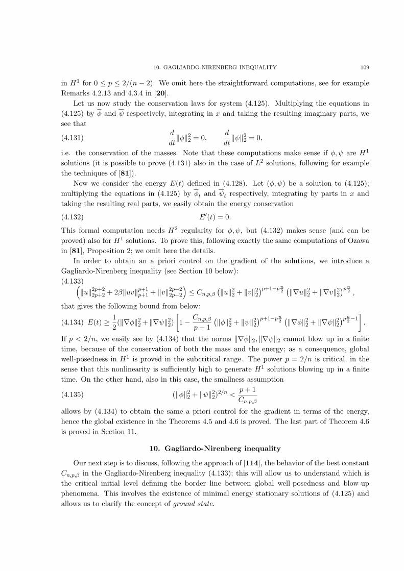
10. GAGLIARDO-NIRENBERG INEQUALITY 109
in H1 for 0 ≤ p ≤ 2/(n − 2). We omit here the straightforward computations, see for exampleRemarks 4.2.13 and 4.3.4 in [20].
Let us now study the conservation laws for system (4.125). Multiplying the equations in(4.125) by φ and ψ respectively, integrating in x and taking the resulting imaginary parts, wesee that
(4.131)d
dt‖φ‖2
2 = 0,d
dt‖ψ‖2
2 = 0,
i.e. the conservation of the masses. Note that these computations make sense if φ, ψ are H1
solutions (it is possible to prove (4.131) also in the case of L2 solutions, following for examplethe techniques of [81]).
Now we consider the energy E(t) defined in (4.128). Let (φ, ψ) be a solution to (4.125);multiplying the equations in (4.125) by φt and ψt respectively, integrating by parts in x andtaking the resulting real parts, we easily obtain the energy conservation
(4.132) E′(t) = 0.
This formal computation needs H2 regularity for φ, ψ, but (4.132) makes sense (and can beproved) also for H1 solutions. To prove this, following exactly the same computations of Ozawain [81], Proposition 2; we omit here the details.
In order to obtain an a priori control on the gradient of the solutions, we introduce aGagliardo-Nirenberg inequality (see Section 10 below):(4.133)(
‖u‖2p+22p+2 + 2β‖uv‖p+1
p+1 + ‖v‖2p+22p+2
)≤ Cn,p,β
(‖u‖2
2 + ‖v‖22
)p+1−p n2(‖∇u‖2
2 + ‖∇v‖22
)p n2 ,
that gives the following bound from below:
(4.134) E(t) ≥ 12(‖∇φ‖2
2 + ‖∇ψ‖22)[1−
Cn,p,β
p+ 1(‖φ‖2
2 + ‖ψ‖22
)p+1−p n2(‖∇φ‖2
2 + ‖∇ψ‖22
)p n2−1].
If p < 2/n, we easily see by (4.134) that the norms ‖∇φ‖2, ‖∇ψ‖2 cannot blow up in a finitetime, because of the conservation of both the mass and the energy; as a consequence, globalwell-posedness in H1 is proved in the subcritical range. The power p = 2/n is critical, in thesense that this nonlinearity is sufficiently high to generate H1 solutions blowing up in a finitetime. On the other hand, also in this case, the smallness assumption
(4.135) (‖φ‖22 + ‖ψ‖2
2)2/n <
p+ 1Cn,p,β
allows by (4.134) to obtain the same a priori control for the gradient in terms of the energy,hence the global existence in the Theorems 4.5 and 4.6 is proved. The last part of Theorem 4.6is proved in Section 11.
10. Gagliardo-Nirenberg inequality
Our next step is to discuss, following the approach of [114], the behavior of the best constantCn,p,β in the Gagliardo-Nirenberg inequality (4.133); this will allow us to understand which isthe critical initial level defining the border line between global well-posedness and blow-upphenomena. This involves the existence of minimal energy stationary solutions of (4.125) andallows us to clarify the concept of ground state.

110 4. NONLINEAR SCHRODINGER EQUATIONS
Consider the functional
Jn,p,β(u, v) =
(‖∇u‖2
2 + ‖∇v‖22
)pn/2 (‖u‖22 + ‖v‖2
2
)p+1−pn/2(‖u‖2p+2
2p+2 + 2β‖uv‖p+1p+1 + ‖v‖2p+2
2p+2
) , u, v ∈ H1;
the infimum of Jn,p,β on H1×H1 is clearly the reciprocal of the best constant Cn,p,β in (4.133).First of all we want to point out that, for any u, v ∈ H1 and for any µ, λ > 0, if we setuµ,λ(x) = µu(λx) and vµ,λ(x) = µv(λx) it follows
‖uµ,λ‖22 = µ2λ−n‖u‖2
2, ‖∇uµ,λ‖22 = µ2λ2−n‖∇u‖2
2,
‖vµ,λ‖22 = µ2λ−n‖v‖2
2, ‖∇vµ,λ‖22 = µ2λ2−n‖∇v‖2
2,
‖uµ,λ‖2p+22p+2 = µ2p+2λ−n‖u‖2p+2
2p+2, ‖vµ,λ‖2p+22p+2 = µ2p+2λ−n‖v‖2p+2
2p+2,
so thatJn,p,β(uµ,λ, vµ,λ) = Jn,p,β(u, v).
Assume that the infimum of Jn,p,β is achieved by (u, v): since the value of the functional isinvariant with respect to the above scalings, we can assume that the best constant in (4.133) isachieved by the pair (u, v) such that(
‖u‖22 + ‖v‖2
2
)=(‖∇u‖2
2 + ‖∇v‖22
)= 1.
Therefore (u, v) is a weak solution of the following system of two weakly coupled ellipticequations
−pn2
∆u+(2− n)p+ 2
2u =
1Cn,p,β
(|u|2p + β|u|p−1|v|p+1
)u
−pn2
∆v +(2− n)p+ 2
2v =
1Cn,p,β
(|v|2p + β|v|p−1|u|p+1
)v,
Now consider the pair (uµ,λ, vµ,λ), corresponding to the choice of parameters
µ =(
2Cn,p,β(2p+ 2− pn)
)1/2p
, λ =(
pn
(2p+ 2− pn)
)1/2
;
this pair solves the following elliptic system
(4.136)
{−∆uµ,λ + uµ,λ =
(|uµ,λ|2p + β|uµ,λ|p−1|vµ,λ|p+1
)uµ,λ
−∆vµ,λ + vµ,λ =(|vµ,λ|2p + β|vµ,λ|p−1|uµ,λ|p+1
)vµ,λ.
Note that the preceding system is variational in nature, so that any (weak) solution is a criticalpoint of the functional
In,p,β(u, v) =12(‖∇u‖2
2 + ‖∇v‖22 + ‖u‖2
2 + ‖v‖22
)− 1
2p+ 2
(‖u‖2p+2
2p+2 + β‖uv‖p+1p+1 + ‖v‖2p+2
2p+2
).
Recently the problem of existence of positive solutions for elliptic systems of this kind hasbeen studied by many authors (see, for example, [4, 7, 35, 71, 74, 96, 120]). In [74] particularattention is given to the existence and some qualitative properties of the ground state solutionsof (4.136): a ground state solution is a nontrivial solution (i.e. distinct from the pair (0, 0))which has the least critical level. In particular it is possible to prove existence of ground statesolutions for system (4.136) solving the following minimization problem
(4.137) inf(u,v)∈N
In,p,β(u, v),
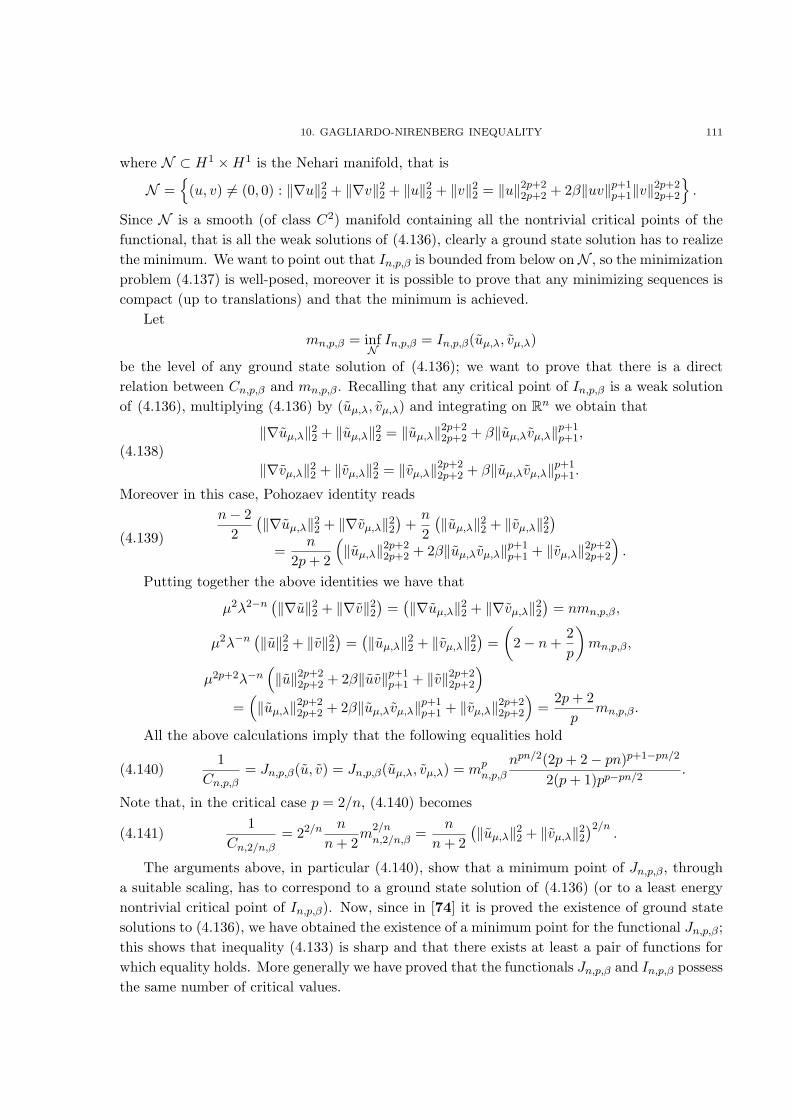
10. GAGLIARDO-NIRENBERG INEQUALITY 111
where N ⊂ H1 ×H1 is the Nehari manifold, that is
N ={
(u, v) 6= (0, 0) : ‖∇u‖22 + ‖∇v‖2
2 + ‖u‖22 + ‖v‖2
2 = ‖u‖2p+22p+2 + 2β‖uv‖p+1
p+1‖v‖2p+22p+2
}.
Since N is a smooth (of class C2) manifold containing all the nontrivial critical points of thefunctional, that is all the weak solutions of (4.136), clearly a ground state solution has to realizethe minimum. We want to point out that In,p,β is bounded from below onN , so the minimizationproblem (4.137) is well-posed, moreover it is possible to prove that any minimizing sequences iscompact (up to translations) and that the minimum is achieved.
Letmn,p,β = inf
NIn,p,β = In,p,β(uµ,λ, vµ,λ)
be the level of any ground state solution of (4.136); we want to prove that there is a directrelation between Cn,p,β and mn,p,β. Recalling that any critical point of In,p,β is a weak solutionof (4.136), multiplying (4.136) by (uµ,λ, vµ,λ) and integrating on Rn we obtain that
(4.138)‖∇uµ,λ‖2
2 + ‖uµ,λ‖22 = ‖uµ,λ‖2p+2
2p+2 + β‖uµ,λvµ,λ‖p+1p+1,
‖∇vµ,λ‖22 + ‖vµ,λ‖2
2 = ‖vµ,λ‖2p+22p+2 + β‖uµ,λvµ,λ‖p+1
p+1.
Moreover in this case, Pohozaev identity reads
(4.139)
n− 22
(‖∇uµ,λ‖2
2 + ‖∇vµ,λ‖22
)+n
2(‖uµ,λ‖2
2 + ‖vµ,λ‖22
)=
n
2p+ 2
(‖uµ,λ‖2p+2
2p+2 + 2β‖uµ,λvµ,λ‖p+1p+1 + ‖vµ,λ‖2p+2
2p+2
).
Putting together the above identities we have that
µ2λ2−n(‖∇u‖2
2 + ‖∇v‖22
)=(‖∇uµ,λ‖2
2 + ‖∇vµ,λ‖22
)= nmn,p,β,
µ2λ−n(‖u‖2
2 + ‖v‖22
)=(‖uµ,λ‖2
2 + ‖vµ,λ‖22
)=(
2− n+2p
)mn,p,β,
µ2p+2λ−n(‖u‖2p+2
2p+2 + 2β‖uv‖p+1p+1 + ‖v‖2p+2
2p+2
)=(‖uµ,λ‖2p+2
2p+2 + 2β‖uµ,λvµ,λ‖p+1p+1 + ‖vµ,λ‖2p+2
2p+2
)=
2p+ 2p
mn,p,β.
All the above calculations imply that the following equalities hold
(4.140)1
Cn,p,β= Jn,p,β(u, v) = Jn,p,β(uµ,λ, vµ,λ) = mp
n,p,β
npn/2(2p+ 2− pn)p+1−pn/2
2(p+ 1)pp−pn/2.
Note that, in the critical case p = 2/n, (4.140) becomes
(4.141)1
Cn,2/n,β= 22/n n
n+ 2m
2/nn,2/n,β =
n
n+ 2(‖uµ,λ‖2
2 + ‖vµ,λ‖22
)2/n.
The arguments above, in particular (4.140), show that a minimum point of Jn,p,β, througha suitable scaling, has to correspond to a ground state solution of (4.136) (or to a least energynontrivial critical point of In,p,β). Now, since in [74] it is proved the existence of ground statesolutions to (4.136), we have obtained the existence of a minimum point for the functional Jn,p,β;this shows that inequality (4.133) is sharp and that there exists at least a pair of functions forwhich equality holds. More generally we have proved that the functionals Jn,p,β and In,p,β possessthe same number of critical values.
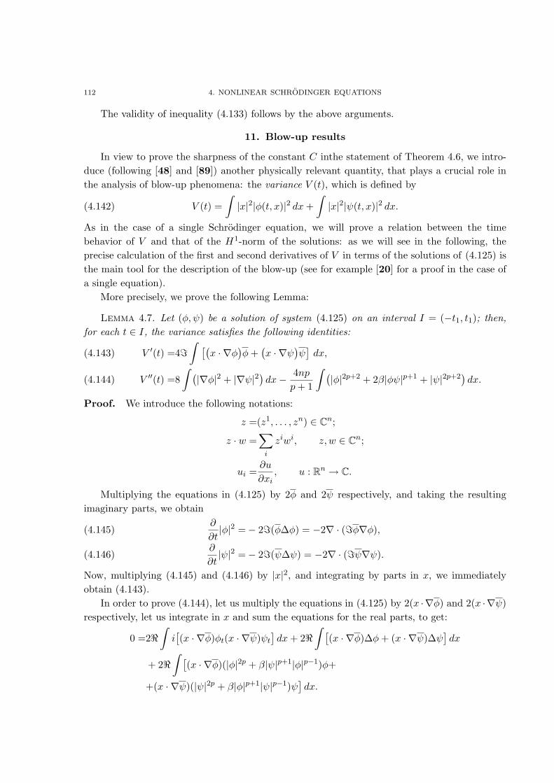
112 4. NONLINEAR SCHRODINGER EQUATIONS
The validity of inequality (4.133) follows by the above arguments.
11. Blow-up results
In view to prove the sharpness of the constant C inthe statement of Theorem 4.6, we intro-duce (following [48] and [89]) another physically relevant quantity, that plays a crucial role inthe analysis of blow-up phenomena: the variance V (t), which is defined by
(4.142) V (t) =∫|x|2|φ(t, x)|2 dx+
∫|x|2|ψ(t, x)|2 dx.
As in the case of a single Schrodinger equation, we will prove a relation between the timebehavior of V and that of the H1-norm of the solutions: as we will see in the following, theprecise calculation of the first and second derivatives of V in terms of the solutions of (4.125) isthe main tool for the description of the blow-up (see for example [20] for a proof in the case ofa single equation).
More precisely, we prove the following Lemma:
Lemma 4.7. Let (φ, ψ) be a solution of system (4.125) on an interval I = (−t1, t1); then,for each t ∈ I, the variance satisfies the following identities:
V ′(t) =4=∫ [(
x · ∇φ)φ+
(x · ∇ψ
)ψ]dx,(4.143)
V ′′(t) =8∫ (
|∇φ|2 + |∇ψ|2)dx− 4np
p+ 1
∫ (|φ|2p+2 + 2β|φψ|p+1 + |ψ|2p+2
)dx.(4.144)
Proof. We introduce the following notations:
z =(z1, . . . , zn) ∈ Cn;
z · w =∑
i
ziwi, z, w ∈ Cn;
ui =∂u
∂xi, u : Rn → C.
Multiplying the equations in (4.125) by 2φ and 2ψ respectively, and taking the resultingimaginary parts, we obtain
∂
∂t|φ|2 =− 2=(φ∆φ) = −2∇ · (=φ∇φ),(4.145)
∂
∂t|ψ|2 =− 2=(ψ∆ψ) = −2∇ · (=ψ∇ψ).(4.146)
Now, multiplying (4.145) and (4.146) by |x|2, and integrating by parts in x, we immediatelyobtain (4.143).
In order to prove (4.144), let us multiply the equations in (4.125) by 2(x ·∇φ) and 2(x ·∇ψ)respectively, let us integrate in x and sum the equations for the real parts, to get:
0 =2<∫i[(x · ∇φ)φt(x · ∇ψ)ψt
]dx+ 2<
∫ [(x · ∇φ)∆φ+ (x · ∇ψ)∆ψ
]dx
+ 2<∫ [
(x · ∇φ)(|φ|2p + β|ψ|p+1|φ|p−1)φ+
+(x · ∇ψ)(|ψ|2p + β|φ|p+1|ψ|p−1)ψ]dx.
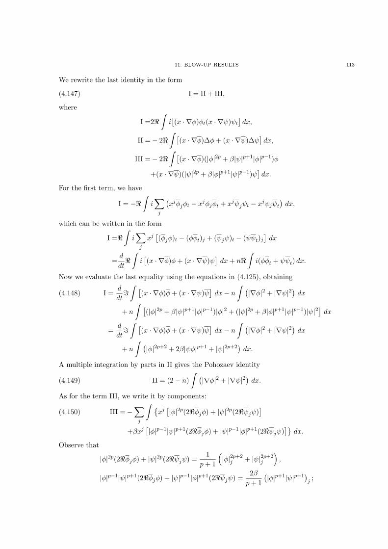
11. BLOW-UP RESULTS 113
We rewrite the last identity in the form
(4.147) I = II + III,
where
I =2<∫i[(x · ∇φ)φt(x · ∇ψ)ψt
]dx,
II =− 2<∫ [
(x · ∇φ)∆φ+ (x · ∇ψ)∆ψ]dx,
III =− 2<∫ [
(x · ∇φ)(|φ|2p + β|ψ|p+1|φ|p−1)φ
+(x · ∇ψ)(|ψ|2p + β|φ|p+1|ψ|p−1)ψ]dx.
For the first term, we have
I = −<∫i∑
j
(xjφjφt − xjφjφt + xjψjψt − xjψjψt
)dx,
which can be written in the form
I =<∫i∑
j
xj[(φjφ)t − (φφt)j + (ψjψ)t − (ψψt)j
]dx
=d
dt<∫i[(x · ∇φ)φ+ (x · ∇ψ)ψ
]dx+ n<
∫i(φφt + ψψt) dx.
Now we evaluate the last equality using the equations in (4.125), obtaining
I =d
dt=∫ [
(x · ∇φ)φ+ (x · ∇ψ)ψ]dx− n
∫ (|∇φ|2 + |∇ψ|2
)dx(4.148)
+ n
∫ [(|φ|2p + β|ψ|p+1|φ|p−1)|φ|2 + (|ψ|2p + β|φ|p+1|ψ|p−1)|ψ|2
]dx
=d
dt=∫ [
(x · ∇φ)φ+ (x · ∇ψ)ψ]dx− n
∫ (|∇φ|2 + |∇ψ|2
)dx
+ n
∫ (|φ|2p+2 + 2β|ψφ|p+1 + |ψ|2p+2
)dx.
A multiple integration by parts in II gives the Pohozaev identity
(4.149) II = (2− n)∫ (
|∇φ|2 + |∇ψ|2)dx.
As for the term III, we write it by components:
III =−∑
j
∫ {xj[|φ|2p(2<φjφ) + |ψ|2p(2<ψjψ)
](4.150)
+βxj[|φ|p−1|ψ|p+1(2<φjφ) + |ψ|p−1|φ|p+1(2<ψjψ)
]}dx.
Observe that
|φ|2p(2<φjφ) + |ψ|2p(2<ψjψ) =1
p+ 1
(|φ|2p+2
j + |ψ|2p+2j
),
|φ|p−1|ψ|p+1(2<φjφ) + |ψ|p−1|φ|p+1(2<ψjψ) =2βp+ 1
(|φ|p+1|ψ|p+1
)j;

114 4. NONLINEAR SCHRODINGER EQUATIONS
hence, integrating by parts in (4.150) we have
(4.151) III =n
p+ 1
∫ (|φ|2p+2 + |ψ|2p+2 + 2β|φ|p+1|ψ|p+1
)dx.
Finally, recollecting (4.147), (4.148), (4.149), (4.151) and (4.143), we complete the proof of(4.144).
Remark 4.8. Note that (4.144) can be rewritten, recalling the definition of E, in the fol-lowing equivalent form
(4.152) V ′′(t) = 16E(t)− 8np− 22p+ 2
∫ (|φ|2p+2 + 2β|φψ|p+1 + |ψ|2p+2
)dx.
In the critical case p = 2/n the equation above reduces to
V ′′(t) = 16E(t);
hence the variance V of any solution of (4.125) with negative initial energy vanish in a finitetime. For each h : Rn → C we can estimate
‖h‖2L2 = ‖|h|2‖L1 ≤ ‖|x|h‖L2
∥∥∥∥ h|x|∥∥∥∥
L2
,
by Cauchy-Schwartz inequality. As a consequence of the standard Hardy’s inequality we obtain
‖h‖2L2 ≤ ‖|x|h‖L2‖∇h‖L2 .
Applying the last inequality to any solution of of (4.125) with negative initial energy, since themass is conserved and the variance vanish in a finite time the L2 norm of the gradient needsnecessarely to blow up in a finite time.
Remark 4.9. Consider the following pair
e−i|x|2−44(1−t)
(1− t)n/2
(U
(x
1− t
), V
(x
1− t
)),
where (U, V ) is a ground state solution of (4.136). This is an explicit example of a blow-upsolution, which shows that Theorem 4.6 is sharp. Indeed the pair solves (4.125) and has initialvalue e−i(|x|2−4)/4(U(x), V (x)) which attains the critical blow-up threshold.
12. On the blow-up threshold
If p = 2/n, we have obtained the following characterization of the blow-up threshold
(4.153)1
Cn,2/n,β=
1Cn,β
=n
n+ 2(‖U‖2
2 + ‖V ‖22
)2/n,
where (U, V ) is a ground state solution of (4.136). In order to prove Theorem 4.6 we have toestimate the quantities involved in (4.153).
In [74] (see Theorem 2.5) it is proved that, if β < 22/n − 1, then any ground state of theelliptic system (4.136) is a scalar function, that is one of the components of the ground statesolution is zero. So we can assume, without loss of generality, that the ground state is (z, 0),where z ∈ H1 is the unique ground state solution (see [114]) of the equation
(4.154) −∆z + z = |z|4n z.

12. ON THE BLOW-UP THRESHOLD 115
This implies that the constant Cn,β = Cn depends only on n for any β ≤ 22/n − 1, sincethe coupling parameter β now does not play a role in the problem of selecting the groundstate solution. Moreover Cn is exactly the blow-up threshold for a single nonlinear Schrodingerequation, introduced and numerically computed in [114].
If β ≥ 22/n−1, Cn,β depends on n and β and its expression is unknown, but we can estimateit using a suitable test-pair. Let z be the unique positive ground state solution of
−∆z + z = (1 + β)|z|4n z,
it is easy to see that the pair (z, z) is a positive solution of (4.136) for any β; and the followinginequality holds
1Cn,β
=n
n+ 2(‖U‖2
2 + ‖V ‖22
)2/n ≤ n
n+ 2(2‖z‖2
2
)2/n.
Clearly we have an inequality since (z, z) could not be a ground state solution of (4.136).Using the scaling as in Section 10 we can estimate Cn,β with Cn. Recalling that z is the
ground state solution of (4.154) and noticing that the L2 norm of z is related to Cn (see (1.3)in [114] and also (4.141)) we obtain that
‖z‖24/n =
‖z‖24/n
1 + β=
n+ 2n(1 + β)Cn
.
Collecting the inequalities above we have
Cn,β ≥(
1 + β
22/n
)Cn,
so that the claim is proved.
Now we give some concluding remarks.
Remark 4.10. Note that it is possible to extend this argument to systems with more thantwo nonlinear Schrodinger equations, using some results about the elliptic counterpart containedin [4], Section 6.


Bibliography
[1] Z.S. Agranovich, V.A. Marchenko, The inverse scattering theory. Gordon and Breach, New York, 1963.[2] S. Agmon, Spectral properties of Schrodinger operators and Scattering Theory, Ann. Sc. Norm. Sup. Pisa Cl.
Sci. 2 (1975) no. 2, 151–218.[3] C. Ahn, Y. Cho, Y., Lorentz space extension of Strichartz estimates, Proc. Amer. Math. Soc. 133 (2005),
no. 12, 3497-3503.[4] A. Ambrosetti, E. Colorado, Standing waves of some coupled nonlinear Schrodinger equations, J. London
Math. Soc. 75 (2007), 67-82.[5] G. Artbazar, K. Yajima, The Lp-continuity of wave operators for one dimensional Schrodinger operators,
J. Math. Sci. Univ. Tokyo 7 (2000), 221–240.[6] J. A. Barcelo, A. Ruiz, L. Vega, Weighted Estimates for the Helmholtz Equation and Some Applications,
J. Funct. Anal. 150 (1997) no.2, 356–382.[7] T. Bartsch, Z.Q. Wang, Note on ground state of nonlinear Schrodinger systems, J. Partial Differential
Equations 19 (2006), 200-207.[8] M. Ben-Artzi, Regularity and smoothing for some equations of evolution. Nonlinear partial differential
equations and their applications. College de France Seminar, Vol. XI (Paris, 1989–1991), 1–12, Pitman Res.Notes Math. Ser., 299, Longman Sci. Tech., Harlow, 1994.
[9] L. Berge, Wave collapse in physics: principles and applications to light and plasma waves, Phys. Rep. 303(1998), 259-370.
[10] J. Bergh, J. Lofstrom, Interpolation spaces. Springer Verlag, Berlin, 1976.[11] M. Beals, Optimal L∞ decay for solutions to the wave equation with a potential Comm. Partial Differential
Equations 19 (1994) no. 7-8, 1319–1369, 1994.[12] M. Beals, W. Strauss, Lp estimates for the wave equation with a potential, Comm. Partial Differential Equa-
tions 18 (1993) no. 7-8, 1365–1397, 1993.[13] N. Burq, Smoothing effect for Schrodinger boundary value problems, Duke Math. J. 123 no. 2 (2004), 403–
427.[14] N. Burq, P. Gerard, N. Tzvetkov, Two singular dynamics of the nonlinear Schrodinger equation on a
plane domain, Geom. Funct. Anal. 13 (2003), 1-19.[15] N. Burq, P. Gerard, N. Tzvetkov, Bilinear eigenfunction estimates and the nonlinear Schrodinger equa-
tion on surfaces, Invent. math. 159 (2005), 187223.[16] N. Burq, F. Planchon, Smoothing and dispersive estimates for 1d Schrodinger equations with BV coeffi-
cients and applications, Preprint 2004.[17] N. Burq, F. Planchon, J. Stalker, S. Tahvildar-Zadeh, Strichartz estimates for the wave and
Schrodinger equations with the inverse-square potential, J. Funct. Anal. 203 (2003) no. 2, 519–549.[18] N. Burq, F. Planchon, J. Stalker, S. Tahvildar-Zadeh, Strichartz estimates for the wave and
Schrodinger equations with potentials of critical decay, Indiana Univ. Math. J. 53(6) (2004), 1665–1680.[19] A. P. Calderon, Spaces between L1 and L∞ and the theorem of Marcinkiewicz Studia Math. 26 (1966),
273–299.[20] T. Cazenave, An introduction to nonlinear Schrodinger equations, Textos de Metodos Matematicos 26,
Universidade Federal do Rio de Janeiro 1996.[21] T. Cazenave, F. B. Weissler, Rapidly decaying solution of the nonlinear Schrodinger equation, Comm.
Math. Phys. 147 (1992), no. 1, 75-100.[22] M. Christ, A. Kiselev, Scattering and wave operators for one-dimensional Schrodinger operators with
slowly decayng nonsmooth potentials, GAFA 12 (2002), 1174–1234.[23] P. Constantin, J.C. Saut Local smoothing properties of Schrodinger equations, Indiana Univ. Math. J. 38
(1989), 791-810.[24] S. Cuccagna, On the wave equation with a potential, Comm. Partial Differential Equations 25 (2000) no.
7–8, 1549-1565.
117

118 BIBLIOGRAPHY
[25] S. Cuccagna, P. Schirmer, On the wave equation with a magnetic potential, Comm. Pure Appl. Math. 54(2001) no. 2, 135–152.
[26] M. Cwikel, On (LP0(A0), LP1(A1))θ,q, Proc. Amer. Math. Soc. 44 (1974), 286-292.
[27] L. D’Ambrosio, S. Lucente, Nonlinear Liouville theorems for Grushin and Tricomi operators, J. DifferentialEquations, 123 (2003) 511-541.
[28] P. D’Ancona, A Note on a Theorem of Jorgens, Math. Z., 218 (1995), 239-252.[29] P. D’Ancona, A. Di Giuseppe, Global Existence with Large Data for a Nonlinear Weakly Hyperbolic Equa-
tion, Math. Nachr., 231 (2001), 5-23.[30] P. D’Ancona, L. Fanelli, Lp-boundedness of the wave operator for the one dimensional Schrodinger oper-
ators, Comm. Math. Phys. 268 (2006), 415–438.[31] P. D’Ancona, L. Fanelli, Decay estimates for the wave and Dirac equations with a magnetic potential,
Comm. Pure Appl. Math. 60 (2007), 357–392.[32] P. D’Ancona, L. Fanelli, Strichartz and smoothing estimates for dispersive equations with magnetic po-
tentials, to appear on Comm. Part. Diff. Eqns.[33] P. D’Ancona, V. Pierfelice, On the wave equation with a large rough potential, to appear on J. Funct.
Anal.[34] A. Di Giuseppe, Global existence with small data for a nonlinear wave equation with time dependent coeffi-
cients, personal communication.[35] D. de Figueiredo, O. Lopes, Solitary Waves for Some Nonlinear Schrodinger Systems, to appear in Ann.
Inst. H. Poincare Anal. Non Lineaire.[36] P. Deift, E. Trubowitz, Inverse scattering on the line, Comm. Pure and Appl. Math. 33 (1979), 121–251.[37] M. B. Erdogan M. Goldberg, W. Schlag, Strichartz and smoothing estimates for Schrodinger operators
with large magnetic potentials in R3, preprint 2006.[38] L. Fanelli, Semilinear Schrodinger equation with time dependent coefficients, to appear on Math. Nach.[39] L. Fanelli, S. Lucente, The critical case for a semilinear weakly hyperbolic equation, El. Journ. diff. eqns.,
Vol 2004(2004), no. 101, 1-13.[40] L. Fanelli, E. Montefusco, On the blow-up threshold for weakly coupled Nonlinear Schrodinger Equations,
J. Phys. A: Math. and Theor. 40 (2007), 14139-14150.[41] G. Fibich, G. Papanicolaou, Self-focusing in the perturbed and unperturbed nonlinear Schrdinger equation
in critical dimension, SIAM J. Appl. Math. 60 (2000), 183-240.[42] D. A. Geba, D. Tataru, Dispersive estimates for wave equations, Comm. Partial Differential Equations
30(4-6) (2005), 849–880.[43] V. Georgiev, A. Stefanov, M. Tarulli, Smoothing - Strichartz estimates for the Schrodinger equation
with small magnetic potential, preprint 2005.[44] V. Georgiev, N. Visciglia, Decay estimates for the wave equation with potential, Comm. Partial Differential
Equations 28 (2003) no. 7-8, 1325–1369.[45] Ginibre, J., and Velo, G., Smoothing properties and retarded estimates for some dispersive evolution
equations, Comm. Math. Phys. 144 (1992), 163–188.[46] J. Ginibre, G. Velo, On a Class of Nonlinear Schrodinger Equations. I. The Cauchy Problem, General
Case, J. Funct. Anal. 32 (1979), 1-32.[47] J. Ginibre, G. Velo, Generalized Strichartz inequalities for the wave equation, J. Funct. Anal. 133 (1995)
no. 1, 50–68.[48] R.T. Glassey, On the blowing up of solutions to the Cauchy problem for nonlinear Schrodinger equations,
J. Math. Phys. 18 (1977), 1794-1797.[49] M. Goldberg, W. Schlag, Dispersive estimates for Schrodinger operators in dimensions one and three,
Comm. Math. Phys. 251 (2004) no. 1, 157–178.[50] M. Goldberg, Dispersive estimates for the three-dimensional Schrodinger equation with rough potentials,
Preprint 2004.[51] M. Goldberg, M. Visan, A counterexample to dispersive estimates for Schrodinger operators in higher
dimensions, Preprint 2005.[52] M. Grillakis, J. Shatah, W. Strauss, Stability theory of solitary waves in the presence of symmetry. I,
J. Funct. Anal. 74 (1987), 160-197.[53] A. Hassell, T. Tao, J. Wunsch, Sharp Strichartz estimates on non-trapping asymptotically conic manifolds,
arxiv.org.[54] F. Hirosawa, M. Reissig, From Wave to Klein-Gordon Type Decay Rates, In “Nonlinear Hyperbolic Equa-
tions, Spectral Theory, and Wavelet transformations”, Oper. Theory Adv. Appl. 145, Birkhauser, Basel,2003, 95-155.

BIBLIOGRAPHY 119
[55] L. Hormander, The analysis of linear partial differential operators II. Grundlehren der MathematischenWissenschaften 257, Springer Verlag, Berlin 1983.
[56] T. Hoshiro, On weighted L2 estimates of solutions to wave equations, J. Anal. Math. 72 (1997) 127-140.[57] A. Jensen, S. Nakamura, Mapping properties of functions of Schrodinger operators between Lp-spaces and
Besov spaces, Adv. Stud. in Pure Math. 23 (1994), 187–209.[58] A. D. Ionescu, D. Jerison, On the absence of positive eigenvalues of Schrodinger operators with rough
potentials, Geom. Funct. Anal. 13 (2003) no. 5, 1029–1081.[59] K. Jorgens, Das Anfangswertproblem in Groem fr eine Klasse nichtlinearen Wellengleichungen, Math. Z.,
77 (1961), 295-308.[60] J.-L. Journe, A. Soffer, C. D. Sogge, Decay estimates for Schrodinger operators, Comm. Pure Appl.
Math. 44 (1991) no. 5, 573–604.[61] K. Kajitani, A. Satoh, Time decay estimates for linear symmetric hyperbolic systems with variable coeffi-
cients and its applications, preprint 2004.[62] T. Kato, Wave operators and similarity for some non-selfadjoint operators, Math. Annalen 162 (1966),
258–279.[63] T. Kato, On nonlinear Schrodinger equations, Ann. I.H.P. Physique Theorique 46 (1987), 113-129.[64] T. Kato, G. Ponce, Commutator estimates and the Euler and Navier - Stokes equations, Comm. Pure
Appl. Math. 41 (1988), 891–907.[65] T. Kato, K. Yajima, Some examples of smooth operators and the associated smoothing effect, Rev. Math.
Phys. 1 (1989), 481–496.[66] M. Keel, T. Tao, Endpoint Strichartz estimates, Amer. J. Math. 120 (1998) no. 5, 955–980.[67] L. D. Landau, E. M. Lifshitz, Course of theoretical physics, Pergamon Press, 1987.[68] M. Lakshmanan, T. Kanna, R. Radhakrishnan, Shape-changing collisions of coupled bright solitons in
birifringent optical fibers, Rep. Math. Phys. 46 (2000), 143-156.[69] R. T. Lewis, Singular Elliptic Operators of Second Order with Purely Discrete Spectra, Trans. Amer. Math.
Soc., 271 (1982), 653-666.[70] O. Liess, Decay estimates for the solutions of the system of crystal optics, Asymptotic Analysis 4 (1991) no.
1, 61–95.[71] T.C. Lin, J. Wei, Ground State of N Coupled Nonlinear Schrodinger equations in Rn, n ≤ 3, Comm. Math.
Phys. 255 (2005) 629-653.[72] S. Lucente, On a class of weakly hyperbolic equations, Annali Univ. Ferrara VII Sci. Mat., vol. LII (2006).[73] S. Lucente, G. Ziliotti, Global existence for a quasilinear maxwell system, Rend. Istit. Mat. Univ. Trieste
31 (2000) suppl. 2, 169–187.[74] L. A. Maia, E. Montefusco, B. Pellacci, Positive solutions for a weakly coupled nonlinear Schrodinger
system, J. Diff. Eqs. 229 (2006), 743-767.[75] J. Maly, L. Pick, An elementary proof of sharp Sobolev embeddings, Proc. Amer. Math. Soc. 130 (2002)
no. 2, 555–563[76] C.R. Menyuk, Nonlinear pulse propagation in birefringent optical fibers, IEEE J. Quantum Electron. 23
(1987), 174-176.[77] F. Merle, P. Raphael, On universality of blow-up profile for L2 critical nonlinear Schrdinger equation,
Invent. Math. 154 (2004), 565-672.[78] F. Merle, P. Raphael, Profiles and Quantization of the Blow Up Mass for Critical Nonlinear Schrodinger
Equation, Comm. Math. Phys. 253 (2005), 675-704.[79] K. Nakanishi, Asymptotically-free solutions for the short range nonlinear Schrodinger equation, SIAM J.
Math. Anal. 32 (2001), no. 6, 1265-1271.[80] R. O’Neil, Convolution operators and L(p, q) spaces, Duke Math. J. 30 (1963), 129–142.[81] T. Ozawa, Remarks on proofs of conservation laws for nonlinear Schrodinger equations, Calc. Var. P.D.E.
25 (2006), 403-408.[82] C. Pladdy, Y. Saito, T. Umeda, Resolvent estimates of the Dirac operator, Analysis 15 (1995) no. 2,
123–149.[83] F. Planchon, On the Cauchy problem in Besov spaces for a non-linear Schrodinger equation, Commun.
Contemp. Math. 2 (2000), no. 2, 243-254.[84] F. Planchon, J. Stalker, S. Tahvildar-Zadeh, Dispersive estimates for the wave equation with the
inverse-square potential, Discrete Contin. Dyn. Syst. 9 (2003), 1387–1400[85] J. Rauch, The u5-Klein-Gordon Equation, In “Nonlinear partial differential equations and their applica-
tions”, Coll. de France Semin., Vol. I, Res. Notes Math. Pitman Research Notes in Math. 53, Pitman 1981,335-364.

120 BIBLIOGRAPHY
[86] M. Reed, B. Simon, Methods of Modern Mathematical Physics vol. I: Functional Analysis. Academic Press,New York, San Francisco, London 1980.
[87] M. Reed, B. Simon, Methods of Modern Mathematical Physics vol. II: Fourier Analysis, Self-Adjointness.Academic Press, New York, San Francisco, London 1975.
[88] L. Robbiano, C. Zuily, Strichartz estimates for Schrodinger equations with variable coefficients, M em. Soc.Math. Fr. 101-102 (2005).
[89] D.C. Roberts, A.C. Newell, Finite-time collapse of N classical fields described by coupled nonlinearSchrodinger equations, Phys. Rev. E 74 (2006), 047602.
[90] I. Rodnianski, W. Schlag, Time decay for solutions of Schrodinger equations with rough and time-dependent potentials, Invent. Math. 155 (2004) no. 3, 451–513.
[91] T. Runst, W. Sickel, Sobolev Spaces of Fractional Order, Nemitskij operators and Nonlinear PartialDifferential Equations, Walther de Gryter, Berlin 1996.
[92] W. Schlag, Dispersive estimates for Schrodinger operators: A survey, preprint 2005.[93] W. Schlag, Dispersive estimates for Schrodinger operators in dimension two, Comm. Math. Phys. 257(1)
(2005), 87–117.[94] J. Shatah, M. Struwe, Regularity Result for Nonlinear Wave Equation, Ann. Math. 138 (1993), 503-518.[95] J. Shatah, M. Struwe, Geometric wave equations. New York University Courant Institute of Mathematical
Sciences, New York, 1998.[96] B. Sirakov, Least Energy Solitary Waves for a System of Nonlinear Schrodinger Equations in Rn, Comm.
Math. Phys. 271 (2007), 199-221.[97] G. Staffilani, D. Tataru, Strichartz estimates for a Schrodinger operator with nonsmooth coefficients,
Comm. Partial Differential Equations 27 (2002) no. 7-8, 1337–1372.[98] A. Stefanov, Strichartz estimates for the magnetic Schrodinger equation, preprint 2004.[99] E. Stein, Harmonic Analysis. Princeton University Press, Princeton, New Jersey, 1993.[100] E. Stein, R. Shakarchi, Complex analysis. Princeton University Press, Princeton 2003.[101] R. Strichartz, Restrictions of Fourier transforms to quadratic surfaces and decay of solutions of wave
equations, Duke Journal of Mathematics, 44 (1977), 705-714.[102] M. Struwe, Semilinear Wave Equations, Bull. Am. Math. Soc., 26 (1992), 53-84.[103] M. Struwe, Globally regular solutions to the u5-Klein-Gordon Equation, Ann. Sc. Norm. Super. Pisa, Cl.
Sci., IV Ser. 15 (1988), 495-513.[104] C. Sulem, P. L. Sulem, The nonlinear Schrodinger Equation. Self-Focusing and Wave Collapse., Springer-
Verlag New York 1999.[105] L. Tartar, Imbedding theorems of Sobolev spaces into Lorentz spaces, Boll. Unione Mat. Ital. Sez. B Artic.
Ric. Mat. (8) 1 (1998) no. 3, 479–500.[106] M. Tarulli Di Giallonardo, Resolvent estimates for scalar field with electromagnetic perturbation, El. J.
Diff. Eqns 2004 (2004), 1-18.[107] M. Taylor, Partial differential equations, Vol. II. Springer, New York 1996.[108] B. Thaller, The Dirac Equation, Springer-Verlag, Texts and Monographs in Physics 1992.[109] P. Sjolin Regularity of solutions to the Schrodinger equation, Duke Math. J., 55 (1987), 699-715.[110] L. Vega Schrodinger equations: pointwise convergence to the initial data, Proc. Amer. Math. Soc. 102
(1988), 874-878.[111] R. Weder, The Wk,p-continuity of the Schrodinger Wave Operators on the line, Comm. Math. Phys. 208
(1999), 507–520.
[112] R. Weder, Lp − Lp′estimates for the Schrodinger equations on the line and inverse scattering for the
nonlinear Schrodinger equation with a potential, J. Funct. Anal. 170 (2000), 37–68.[113] R. Weder, The Lp − Lp Estimate for the Schrodinger Equation on the Half-Line, J. Math. Anal. Appl.
281 (2003), 233–243.[114] M.I. Weinstein, Nonlinear Schrodinger Equations and Sharp Interpolation Estimates, Comm. Math. Phys.
87 (1983), 567-576.[115] K. Yajima, The W k,p-continuity of wave operators for Schrodinger operators, J. Math. Soc. Japan 47
(1995), 551–581.[116] K. Yajima, The W k,p-continuity of wave operators for Schrodinger operators III, even dimensional cases
m ≥ 4, J. Math. Sci. Univ. Tokyo 2 (1995), 311–346.[117] K. Yajima, Lp-boundedness of wave operators for two-dimensional Schrodinger operators, Comm. Math.
Phys. 208 (1999), 125–152.[118] K. Yajima, Dispersive estimate for Schrodinger equations with threshold resonance and eigenvalue, Comm.
Math. Phys. 259 (2005), 475–509.

BIBLIOGRAPHY 121
[119] O. Yamada, On the principle of limiting absorption for the Dirac operators, Publ. Res. Inst. Math. Sci. 8(1972/73), 557–577.
[120] J. Yang, Classification of the solitary waves in coupled nonlinear Schrodinger equations, Phys. D 108(1997), 92-112.