Are Bank Shareholders Enemies of Regulators or a Potential Source of Market Discipline?

Sangkyun Park and Stavros Peristiani*

Abstract: In moral hazard models, bank shareholders have incentives to transfer wealth from thedeposit insurer --that is, maximize put option value-- by pursuing riskier strategies. For safe banks withlarge charter value, however, the risk-taking incentive is outweighed by the possibility of losing chartervalue. Focusing on the relationship between book value, market value, and a risk measure, this paperdevelops a semi-parametric model for estimating the critical level of bank risk at which put option valuestarts to dominate charter value. From these estimates, we infer the extent to which the risk-takingincentive prevailed during 1986-92, a period characterized by serious banking problems and financialturmoil. We find that despite the difficult financial environment, shareholders’ risk-taking incentive wasconfined primarily to a small fraction of highly risky banks.

SANGKYUN PARK is an Economist at the Office of Management and Budget. STAVROSPERISTIANI is a Research Officer in the Research and Market Analysis Group of the Federal ReserveBank of New York.

*Corresponding author, Main 3 East, Federal Reserve Bank of New York, 33 Liberty Street, NewYork, NY 10045. E-mail: steve.peristiani@ny.frb.org. We wish to thank Gijoon Hong for excellentresearch assistance. The views expressed in this paper are those of the authors and do not necessarilyrepresent the views of the Federal Reserve Bank of New York, the Federal Reserve System or theOffice of Management and Budget.

1

1. INTRODUCTION

Many regulators and academic researchers have emphasized market discipline as a means

to improve the safety and soundness of the banking system. Perhaps this cannot be more true

than in today’s complex financial landscape. Because of ever increasing complexity of the

banking business, it is difficult to effectively regulate banks solely based on prescribed rules.

The importance of market discipline is underscored by the recent banking and financial crises in

several emerging markets as well as more industrialized countries worldwide. In many instances,

the inability of bank regulators and market forces to effectively discipline financial institutions

was deemed as the missing ingredient for ensuring financial stability. Not surprisingly, in the

last few years we have been witnessing a renewed interest among policy makers in enacting

changes that would encourage more market disclosure and transparency. The new capital

adequacy proposals of the Basel Committee for Banking Supervision consider market discipline,

along with capital requirements and supervision, as one of the three pillars to support the banking

system. Furthermore, directed by the Gramm-Leach-Bliley Act of 1999, the U.S. Treasury and

the Federal Reserve Board are considering using mandatory subordinated debt as a catalyst to

strengthen market discipline.

The interest in market discipline has largely been stimulated by the moral hazard

literature describing the conflict between shareholders and debtholders (or the deposit insurer in

the case of insured banks). In a moral hazard framework, bank managers act in the interest of

shareholders, who have voting power. Shareholders with limited liability have a put option, that

is, have the right to sell the bank’s assets at the face value of its liabilities. The value of the put

option increases with the bank’s risk, typically, reflected by a larger variance of the asset

2

portfolio and a lower capital ratio. If the shareholders of a bank are interested mainly in the put

option value, managers may accommodate them by increasing the bank’s risk. In this case,

shareholders are enemies of bank regulators, and the burden of market discipline falls on the

shoulders of debtholders.

Several studies of moral hazard have shown that bank shareholders are also responsive to

the bank’s charter value or intangible capital (e.g., Marcus (1984), Keeley (1990), Ritchken et al.

(1993), and Park (1997)). In the event of failure, shareholders have to forfeit charter value.

Their incentive to preserve the charter value should therefore outweigh their desire to increase

the put option value when the bank’s risk is low or moderate, while the opposite is true at high

levels of risk. Consequently, bank shareholders can be allies of regulators or a source of market

discipline when a bank is reasonably safe.

The moral hazard theory raises an intriguing empirical question: At what level of risk do

shareholders turn to enemies of regulators? Several empirical studies have attempted to shed

some light on the relative importance of put option value and charter value. Most notably,

Keeley’s (1990) study attributes the sharp rise in failure among banks and thrift institutions to the

gradual deterioration of bank charter value. Keeley argues that rapid deregulation of the banking

and thrift sectors during the 1980s coupled with intense competition from nonbank institutions

engendered a deterioration in the charter value of banks and thrifts. As a result of lower charter

value, shareholders were compelled to switch to riskier strategies, which in turn brought about

the increased incidences of bank failure in this period. Brewer and Mondschean (1994) compare

the behavior of low- and high-capital savings and loan associations (S&Ls). Their analysis finds

that poorly capitalized S&Ls exhibit a positive relationship between stock market returns and

3

junk bond holdings. This result indicates that the market may be looking favorably at high-risk

strategies for firms whose option value is likely to be higher than charter value. Demsetz,

Saidenberg and Strahan (1996) explore more directly the relationship between franchise value

and bank risk. The authors find a negative relationship between charter value and different stock

market measures of risk. In line with theoretical predictions, they also discover that banks with

higher charter values are motivated to take safer strategies and tend to hold more capital.

This paper differs from the previous empirical studies in that we focus on the tradeoff

between the put option value and charter value in relation to the level of bank risk. In particular,

our analysis aims to highlight the bipolar behavior of bank shareholders -- on one hand, as allies

of regulators, protecting their stake in a low-option value institution by penalizing risky

strategies, and on the other hand, as enemies of regulators, condoning more risk-taking strategies

for institutions whose option value outweighs charter value.

In this paper, we gauge bank risk by the failure probability estimated from actual bank

failure records. Condensing the measure of risk into a single dimension greatly simplifies our

analysis. The option value and the charter value are jointly inferred from the ratio of the market

value of the firm to the book value of its assets (commonly referred to as the Q ratio). A negative

relationship between the failure probability and the Q ratio would mean that the expected loss of

the charter value outweighs the increase in the option value, and a positive relationship would

indicate the opposite. As we will illustrate in the next section, the theoretical relationship

between bank risk and the Q ratio is nonlinear and convex, reflecting the changing relative

importance of charter value and put option value. Moral hazard theory, however, establishes the

functional relationship between bank risk and market-to-book value without the explicit benefit

4

of a structural model with a well defined parametric form. We resolve this challenge by using a

semi-parametric spline estimation technique to estimate the link between bank risk and the Q

ratio.

The principal findings of our analysis are interesting in several respects. For one, we

discover that the threshold at which the marginal contribution of the option value starts

outweighing the expected loss of the charter value is around the 17-percent annual probability of

failure. This point of transition is at a fairly high level because only a very small fraction of

bank holding companies (roughly 3 percent) attain failure scores that are greater than this

threshold level. Second, looking at a group of high-charter banks (characterized by a strong core

deposits base), we find that the Q ratio for these institutions decreases at a higher level of the

failure probability. This result is consistent with the theoretical prediction that banks with more

valuable charters are more averse to risk. Overall, our analysis suggests that moral hazard arising

from the shareholder-debtholder conflict was confined to a tiny subset of banks. Shareholders

are therefore mostly a source of discipline on incompetent and self-serving managers.

The rest of the paper is organized as follows. The next section presents a simple moral

hazard model that demonstrates the expected relationship between the failure probability and the

Q ratio. In the third section, we estimate the failure probability and its effect on the Q ratio. The

final section summarizes the paper’s findings.

1Unless the insurance premium fully reflects the riskiness of banks, risk-based premiumswould not change the qualitative results. Chan et al. (1992) show that “fair” pricing of depositinsurance is not possible under some plausible conditions.

5

2. EFFECTS OF FAILURE RISK ON SHAREHOLDERS’ WEALTH

A simple two-period model in this section shows the effect of bank risk on the option

value and the charter value and the expected relationship between the failure probability and the

Q ratio. In the model, the portfolio choice and the capital ratio determine the shareholders’

wealth by affecting the put option value and the charter value. In many ways, our framework is

very similar to theoretical models developed by Marcus (1984), Keeley (1990), Ritchken et al.

(1993), and Park (1997). Nevertheless, this section has two useful purposes. First, it provides

the reader a brief overview of the traditional moral hazard framework. More important, this

simple theoretical model allows us to formally establish the nonlinear tradeoff between market-

to-book value and bank risk.

2.1. Financial Structure of Banks

The liability of banks consists solely of deposits that are fully insured by the government.

Since the government-insured deposits are riskless, banks offer the risk-free rate of return on

deposits. For simplicity, the insurance premium is assumed to be zero.1

In this two-period model, banks invest deposits and their own capital at the beginning of

period 1, and the outcome of the investment becomes known at the beginning of period 2. Two

investment projects are available for banks; one is risk-free (e.g., short-term Treasury securities),

and the other is risky (e.g., loans). All agents are assumed to be risk neutral. The gross rate of

return on the risk-free investment is R per period, which is 1 plus the risk-free rate of return. The

6

D×R > (1�α) (D�K)R � α (D�K)ζ, (1)

ζ< (α�κ)Rα

� ζ�, (2)

p � �ζ�

0

g(ζ) dζ, (3)

return from the risky project is a random variable that is distributed between 0 and u with the

expected value R. Thus, both investments are zero net present value (NPV) projects.

2.2. Probability of Failure

A bank fails if its liability exceeds the asset at the beginning of the second period. For

simplicity, liquidation is assumed to be costless. Algebraically, a bank fails if:

where is the amount of deposits in period 1; is the amount of capital in period 1; is theD K ζ

realized return from the risky investment; and is the proportion of the bank's assets invested inα

the risky project. Solving (1) for , we find that the bank fails if:ζ

where is the capital ratio, that is, . κ K(D�K)

Since is a random variable, the probability of failure is defined as:ζ

where is the probability density function of . It is rather intuitive that this probabilityg(ζ) ζ

increases with and decreases with (see Park, 1997, for a more formal presentation).α κ

7

E(W) � �ζ�

0

0g(ζ)dζ�A�u

ζ�

[αζ�(1�α)R � (1�k)R]g(ζ)dζ, (4)

E(W) � κ×A×R � pA �(1�k)R�[(1�α)R � αE(ζ�ζ<ζ�)]�. (5)

OV � pA �(1�k)R � [(1�α)R � αE(ζ � ζ<ζ�)]� � p × AD. (6)

2.3. Put Option Value

Limited liability of shareholders produces a put option value. With limited liability, the

expected wealth of shareholders is

where represents total asset . Shareholders with limited liability receive nothing ifA (D�K)

equity becomes negative , otherwise they keep positive equity . Equation (4) can be(ζ�ζ�)

expressed as:

Here, represents the expected return from the risky project provided that is smallerE(ζ�ζ< ζ�) ζ

than , i.e., that the bank fails.ζ�

Since is the opportunity cost or the intrinsic value of capital, the option value(k×A×R)

arising from limited liability is defined as:

The option value is the failure probability times the expected asset deficiency (e.g., liabilityAD

minus asset) in the event of failure, which equals the expected loss of the deposit insurer. Since

both risky and riskless investments are zero net present value (NPV) projects, no one can gain in

expected value terms unless someone else loses. Thus, the expected loss of the insurer is the

expected gain of bank shareholders. It is a well known result that increases with andOV α

8

E(WC) � �ζ�

0

0×g(ζ) dζ � A�u

ζ�

[αζ � (1�α)R� (1�κ)R] g(ζ)dζ

��u

ζ�

CVg(ζ)dζ � κ×A×R � pD � (1�p)CV,

(7)

OVC � p (AD�CV). (8)

decreases with (Keeley, 1990; Marcus, 1984; Park, 1997; and Ritchken et al., 1993). Both κ p

and increase with and decrease with AD α κ

2.4. Charter Value

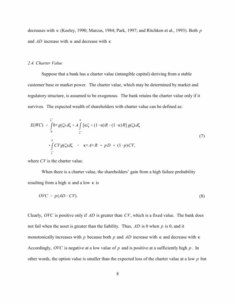
Suppose that a bank has a charter value (intangible capital) deriving from a stable

customer base or market power. The charter value, which may be determined by market and

regulatory structure, is assumed to be exogenous. The bank retains the charter value only if it

survives. The expected wealth of shareholders with charter value can be defined as:

where CV is the charter value.

When there is a charter value, the shareholders’ gain from a high failure probability

resulting from a high and a low isα κ

Clearly, is positive only if is greater than , which is a fixed value. The bank doesOVC AD CV

not fail when the asset is greater than the liability. Thus, is 0 when is 0, and itAD p

monotonically increases with because both and increase with and decrease with p p AD α κ

Accordingly, is negative at a low value of and is positive at a sufficiently high . InOVC p p

other words, the option value is smaller than the expected loss of the charter value at a low butp

2The book value may differ from the value of tangible capital because of inaccuratedepreciation schedule and delayed loss recognition. Although depreciation schedule is unlikelyto be correlated with the failure probability, the unrecognized loss may be positively related tothe failure probability. Thus, the empirical section controls for the unrecognized loss.

9

MV � BV � CV � OVC � N. (9)

outweighs the expected loss at a high . The shareholders’ wealth, therefore, decreases with p p

at first but reverses direction beyond a critical level at which . This inflection pointAD�CV

depends on the relative magnitude of the charter value and the option value.

2.5. Market Value Versus Book Value

The relative importance of the charter value and the option value of a bank can be

inferred from the relationship between the failure probability, the market value, and the book

value of the bank’s capital. The shareholders’ wealth consisting of tangible capital , the(k×A×R)

option value, and the charter value should be equal to the market value of the bank’s stock. In

contrast, the book value of capital does not normally include the option value and the charter

value of the bank.

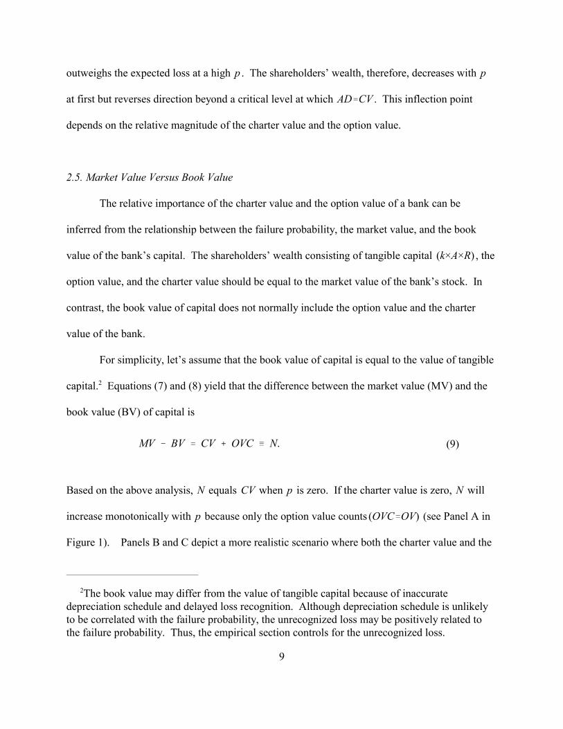
For simplicity, let’s assume that the book value of capital is equal to the value of tangible

capital.2 Equations (7) and (8) yield that the difference between the market value (MV) and the

book value (BV) of capital is

Based on the above analysis, equals when is zero. If the charter value is zero, will N CV p N

increase monotonically with because only the option value counts (see Panel A inp (OVC�OV)

Figure 1). Panels B and C depict a more realistic scenario where both the charter value and the

3The graphical illustrations provided in Figure 1 assume that is uniformly distributedζbetween 0 and , , , and . To change the level of bank risk, we vary the2R R�1.05 A�10 k�0.05value of between 0 to 1. Our example assumes a uniform distribution for analytical simplicity. αBecause the uniform distribution assigns an equal chance in the interval between (an[0,2R]extreme case of fat tails and hence very high option values), one of the simulation examplesrequires a fairly large charter value (150) to generate a steadily declining nonlinear relationshipbetween shareholder wealth and risk.

4For a bank with positive capital, the failure probability cannot be greater than 0.5 if itinvested in a zero NPV project with a symmetric return distribution.

10

option value matter. In these examples, decreases with at first and begins to rise with N p p

beyond a critical level, which represents the point at which the marginal expected loss of the

charter value equals to the marginal expected gain in the option value. The inflection point of p

depends on the initial magnitude of the charter value holding other parameters constant. Panel D

illustrates the other extreme scenario of a bank with very large charter value. Here, it is possible

that decreases with in the entire range of observable values, meaning that high-charterN p

institutions have the most to lose from gambling on risky strategies.3

The risky investment in the above analysis is a zero NPV project. In reality, an extremely

high failure probability may be caused by negative NPV projects.4 If this is the case, may stopN

rising or start decreasing again at a high because negative NPV projects decrease thep

shareholders’ wealth. A heavy regulatory burden on high-risk banks may also limit the increase

in .N

5Alternatively, this Q ratio measure equals {1 + (market value of equity - book value ofequity) / book value of assets}.

11

Qti � f(pti) � β Zti� � εti. (10)

3. A SEMI-PARAMETRIC MODEL FOR DETERMINING MARKET-TO-BOOK VALUE

3.1 An Empirical Model

Equation (9) provides a simple framework for estimating the relationship between charter

value, option value, and bank risk. Essentially, the value of a banking firm net of the opportunity

cost of capital (extra value) consists of the charter value plus the option value. In reality, neither

component of the extra value is observable. Instead, as illustrated quite vividly by the graphical

examples (Figure 1), one can infer a certain behavioral association between risk-taking and the

two components of bank value. In the more realistic scenario, we hypothesize that both charter

value and option value contribute to extra value.

Our empirical model is designed to capture the nonlinear and convex relationship

between shareholders’ wealth and bank risk. Like Keeley (1990) and Demsetz et al. (1997), we

measure the sum of the option value and the charter value by the Q ratio. More specifically, the

dependent variable in our analysis is the sum of the market value of equity and the book value of

liabilities divided by the book value of assets net of goodwill.5 The nonlinear relationship

between the Q ratio and its determinants are specified as the following semi-parametric model:

The key control in our nonlinear regression model is a variable measuring a bank’s risk . We(pti)

assume that the nonlinear relationship between a bank’s Q ratio and risk is determined by the

unknown function . f(�)

12

In addition to the non-parametric relationship between the Q ratio and , the empiricalpti

model includes other variables that may influence the Q ratio, defined by the vector . InZti

particular, the vector includes the log of asset size , core deposits as a percent of assets(ASSETti)

, commercial and industrial loans as percent of assets , delinquent assets(COREti) (CILOANSti)

as a fraction of loan loss reserves , and year dummies. CORE (loyal depositor base)(DELQTti)

and CILOANS (lending relationship) are included to capture cross-sectional variation in charter

value. The variable CORE is expected to have a positive effect on the Q ratio. The effect of

CILOANS, however, is ambiguous. At one level, lending relationships in banking can be viewed

as an important contributor to charter value. However, banks lending to businesses face

significant risks because commercial and industrial loans are often unsecured. Thus, an

excessive concentration of business loans may be viewed as a high-risk strategy and may also be

positively correlated with bank risk. The variable ASSET is a useful regressor because it can

potentially affect both the option value and the charter value; larger option value for larger banks

because of the “too-big-to fail” policy or larger charter value for larger banks because of more

market power and banking expertise. In either case, the sign of the variable is likely to be

positive. The variable DELQT is included in the model to capture hidden losses that would

negatively affect the Q ratio by unduly inflating the book value of equity. Finally, the

specification includes year dummies to capture varying stock market conditions over time.

3.2 Measuring Bank Risk by the Likelihood of Failure

The key explanatory factor in our analysis is a measure of bank riskiness . Previouspti

studies have taken different approaches to measuring bank risk relying on stock market based

13

y �

t i � xt�1, i�γ � υt i, (11)

measures of volatility or simply using capital ratios. In this paper, we construct a bank-specific

measure of solvency. A number of empirical papers in the literature on market discipline have

shown that statistical models can provide accurate ex ante measures of bank solvency (see

Gilbert (1987) for a review of the literature). Typically, these studies construct a score of bank

riskiness from historical failure information. Using a model of discrete choice, the dependent

variable (failure or nonfailure) would be regressed on the financial characteristics of the bank.

Recent studies have employed more elaborate econometric methods such as proportional hazard

models or survival analysis with competing risks (Cole and Gunther (1995)). Despite the added

level of complexity, these sophisticated models provide comparatively similar forecasting results.

In this study, we employ logistic regression to estimate the probability of failure for

banks. The premise in market discipline is that market participants (depositors, shareholders,

debtholders, and regulators) need to estimate the solvency of the depository institution from

publicly available information. Our goal in this paper is somewhat similar in the sense that we

seek to construct a measure of bank solvency that would accurately describe the current state of

the institution. Often studies of bank failure concentrate on long time horizons because their

main concern is evaluating failure prediction models for regulatory purposes. Regulators must

recognize the likelihood of failure as early as possible to be able to take preventive or corrective

action. In comparison, our framework is focused more on capturing the near-term behavior of

the bank. The logistic regression can be defined as:

14

yti � 1 if y �

t i � 0 (bank failure in t),yti � 0 if y �

t i > 0 (otherwise),

p̂ti � F(xti�;γ̂(t�1)), (12)

where

such that is a vector of financial characteristics of the bank in year (t-1). The dependentxt�1, i�

variable can be viewed as a latent index of bank solvency. Note that the logit model isy �

t i

estimated using information as of period because in most cases we do not have complete(t�1)

information on bank failures in the current year . Based on this model we estimate the(t)

financial health of the bank using financial information as of year . In particular, a forward-(t)

looking estimate of the likelihood of failure can be computed from

where represents the logistic distribution, and the superscript simply indicates thatF(�) (t�1)

model was estimated based on information from the previous year.

The logit model is estimated yearly for the period 1985-92. A large fraction of the bank

mergers in the 1980s were engineered by regulators to salvage poorly performing banks. To

avoid possible sample bias, we eliminated from our data all banks that were taken over during

the period (except of course for FDIC-assisted mergers that were counted as failures). Although

ultimately this paper investigates the relationship between charter value and bank riskiness at the

bank holding company (BHC) level, our prediction model for bank failure is estimated at the

bank level. It is practically impossible to accurately measure failure risk at the holding company

level because there were only a handful of publicly traded companies that failed. In contrast,

6We use total assets of the bank as weight for calculating the holding company scores. Wehave also experimented with alternative measures such as assigning to the BHC the score of itslead subsidiary. Overall, the results were very similar.

15

during 1985-92, there were roughly 1,200 bank failures. Thus, it is much easier to construct a

score of failure for bank subsidiaries than for their bank holding parent. An estimate of

probability of failure for the BHC is simply given by the weighted average of score of all its

subsidiaries.6

The explanatory variables consists of mainly financial ratios measuring thext�1, i�

fundamental risks of financial intermediation, which are typically used by regulators and

investors to evaluate the safety and soundness of banks. The set of explanatory variables

includes for instance measures of capital adequacy, asset quality, management quality,

profitability, and liquidity.

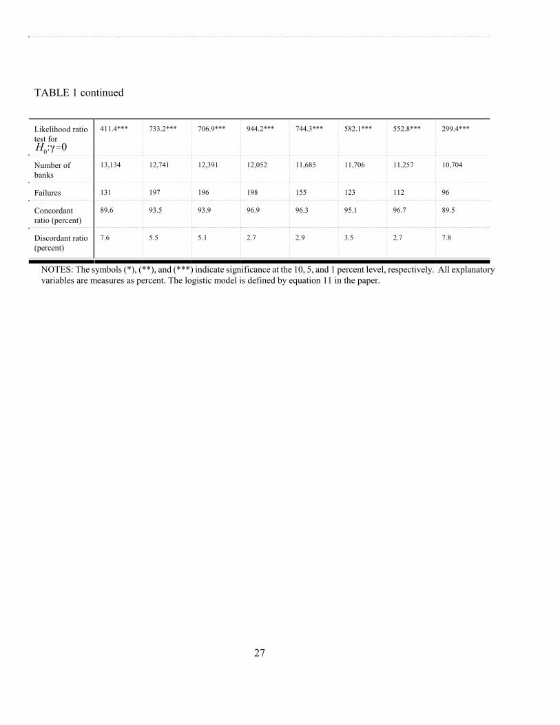
Table 1 presents estimates of the logistic regression for the period 1985-92. Although

coefficients are not always significant, they do exhibit the expected sign in most cases. As seen

from the table, measures of capital adequacy play a critical role in determining bank failure.

More important to our analysis, the logit models generate fairly accurate and reliable forecasts of

failure. The concordant ratio for most of the estimated logit regressions is close to or over 90

percent, meaning that model is able to classify correctly most of the observed responses.

Moreover, the different logistic regressions across time provide time-consistent forecasts in the

sense that the probability of failure for an insolvent bank rises significantly before it is closed by

regulators.

16

4. EFFECT OF THE FAILURE PROBABILITY ON THE MARKET-TO-BOOK RATIO

4.1 Data

Our data is an unbalanced sample of 337 publicly traded BHCs, with a total of 1,902

bank-year observations spanning the period 1986-92. To calculate the Q ratio for BHCs, we use

market value information from Standard and Poor’s COMPUSTAT database. As noted

previously, an estimate of the failure probability is produced at the bank level using information

from the Consolidated Report of Condition and Income for Banks (Call Reports), which is

available at the Board of Governors. The remaining information was obtained from the

Consolidated Financial Statement for Bank Holding Companies (FR Y-9C), also available from

the Board of Governors.

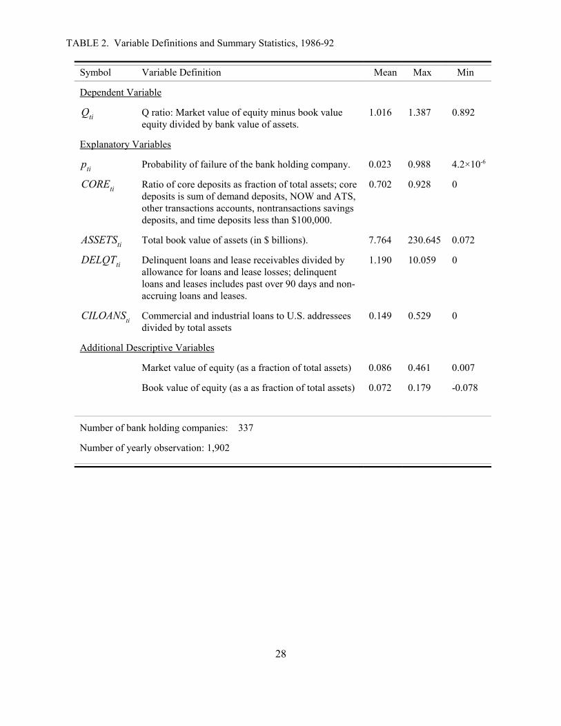
Table 2 provides summary statistics of the regression variables explaining the Q ratio

defined by equation (10). In line with other studies of firm value, our Q ratio averages close to

1.016. On the surface, the mean probability of failure in a given year is fairly high at 0.023. But

this of course is driven primarily by a handful of failing institutions with very large scores. The

median of the probability of failure is roughly 0.0056, meaning that the distribution of the

estimates of failure is skewed to the right.

4.1 The Nonlinear Effect of Bank Risk

We employ three different approaches to estimating the functional relationship between

firm value and bank risk defined by equation (10). The first empirical model asserts that isf(pti)

a simple linear function of the probability of failure. The second approach specifies as af(pti)

third-order polynomial. These two simplifications of our empirical model serve basically as

17

ESS� 1N�

T

t�1�N

i�1(Qti�f (pti)�β Zti�)

2. (13)

1N�

T

t�1�N

i�1(Qti�f (pti)�β Zti�)

2� λ�

b

a

( f (2)(p))2dp. (14)

convenient baselines against which we can compare the more complex spline estimator. In

contrast to linear specifications that minimize the error sum of squares of the model, the semi-

parametric spline estimator optimizes the error sum of squares as well as the “smoothness” of the

functional solution. More specifically, both the polynomial and linear estimators minimize

In comparison, the spline approach optimizes the tradeoff between ESS and a measure of the

“smoothness” of . In its simplest form, the minimization criterion can be defined as thef (pti)

sum of ESS plus a second component representing the penalty of roughness times the smoothing

parameter . Specifically,λ

Here, the roughness of is defined by the integral of the square of the second derivative off (�)

. The parameter determines the tradeoff between smoothness and goodness of fit. Anf (�) λ

excellent survey of the spline models, describing methods of estimation and other applications, is

given in Wahba (1990).

The first two columns of Table 3 present least square estimates of the simple parametric

versions of the model. In the linear case, the estimate coefficient value of is negative,pti

suggesting that the Q ratio continues to decline at higher levels of bank risk. The inadequacy of

the simple linear model is further underscored by the notable improvement in the fit of the

18

polynomial model. All of the three terms turn out to be statistically significant at the 1 percent

level. The estimates reveal a fairly strong nonlinear relationship between the Q ratio and the

failure probability.

Although the third-order degree polynomial provides a fairly good fit, a major limitation

of this approach is that it imposes an arbitrary functional specification. The spline model

resolves the estimation problem by evaluating both the nonparametric and parametric facets of

the model. In the third column, the root mean square error of the spline model is now slightly

larger than the polynomial model because this approach optimizes a different and broader

criterion.

Because the spline estimator for is nonparametric, the best way to demonstrate itsf (pti)

contribution is through a graph. Figure 2 plots the relationship between the Q ratio and the

probability of failure , assuming that the remaining parametric explanatory variables aref (pti)

evaluated at their mean. The figure clearly reveals a nonlinear pattern that is consistent with

theory and our simulation examples. The shape of the empirical spline function implies that both

charter value and put option value matter in the valuation of the bank. In line with a couple of

our theoretical simulation scenarios presented in Figure 1 (specifically Panels B and C), we

observe that at first the Q ratio declines with the increasing likelihood of failure. The Q ratio

gradually reaches a minimum after which it reverses direction and begins to rise again. The

reversal in the estimated Q ratio function allows us to locate the level of riskiness at which the

put option value of the insurance subsidy begins to dominate the loss of charter value.

7This probability threshold is pertinent only for the annualized logit regression model. As willbe shown later, the risk metric will be different for quarterly logistic regressions or for someother appropriate sample design variation.

19

Based on our full sample of BHCs, our results indicate that the critical threshold of

transition is around a yearly probability of failure of 0.17.7 It is interesting to note that roughly

3 percent of the bank observations in our sample have a failure probability higher than the

17-percent level threshold. This result suggests that shareholders had incentives to encourage

managers to pursue riskier strategies in only a handful of cases during the sample period. The

identification of the threshold probability also has an important implication for prompt corrective

action. In 1991, the FDIC Improvement Act (FDICIA) has introduced a range of prompt

corrective action rules requiring mandatory closure of banks failing to meet certain regulatory

standards. The primary objective of these prompt corrective action criteria is to minimize the

damages from insolvency. Interestingly, implicit in the prompt corrective action rules

implemented by FDICIA is the belief that bank regulators can close down a failing bank before it

goes beyond the turning point where the put option value exceeds the franchise value of the firm.

Perhaps the most intriguing implication of our empirical analysis is that risk is quite

detrimental to charter value. Safer banks are the ones with most to lose from higher risk. As

illustrated by Figure 2, investors are initially averse to risk-taking as any significant sign of

deteriorating financial conditions is readily disciplined. The aftermath of a more conspicuous

jump in the likelihood of failure (say from around zero to 0.05) is typically a sharp deterioration

in the bank’s Q ratio to typically below one. The high threshold level and the strong negative

relationship between bank risk and shareholders’ wealth for safe banks signify that regulators can

count on bank shareholders as a source of market discipline to a large extent.

20

The remaining parametric explanatory variables have the right sign and are usually

statistically significant. The strong explanatory power of DELQT may reflect bank managers’

incentives to delay the recognition of losses and to inflate the book value of capital. The

significance of CORE indicates a wide variation in charter value across banks.

Moral hazard theory predicts that the probability threshold at which the put option

overtakes charter value would be higher for banks with greater charter value. Given its empirical

significance, CORE seems to be a good proxy for charter value. Banks with higher core deposit

ratios are more likely to have greater charter values. We divide the sample into two groups of

equal size based on CORE (high-CORE and low-CORE banks). The two sub-samples produce

significantly different functional relationships between the failure probability and the Q ratio.

The probability transition threshold is smaller for low-CORE banks than that for their high-

CORE counterparts. This outcome affirms that the desire to take on more risk was probably

stronger among BHCs with weaker core deposit base. Having smaller charter values, these banks

have less to lose and are more likely to realize the marginal benefits of insurance subsidy from

taking on more risk. Perhaps as important is our finding that the nonlinear relationship between

risk and the Q ratio for high-CORE banks exhibits limited marginal benefits from greater risk as

it rises at much lower trajectory. Shareholders of high-CORE banks are therefore more reluctant

to accept riskier strategies that deplete charter value.

4.2 Robustness of Results

The surge in failures during the latter half of the 1980s was primarily concentrated in

smaller banks and thrifts. In reality, only a very small fraction of publicly traded bank holding

21

companies have actually failed in United States during this period, although several of the

weaker banks found refuge by merging with healthier institutions. Specifically, our panel of

BHCs includes only three failures. In part, our analysis has dealt with the rarity in BHC defaults

by estimating riskiness at the bank subsidiary level. Overall, we found that the likelihood of

failure for BHCs is quite small. Roughly 90 percent of bank observations had a probability of

failure less than 0.04. Put another way, the estimated semi-parametric function was determined

to a great length by a small fraction of bank observations with significant probabilities of failure.

The skewness in the distribution of failure scores raises a concern that our results may not

be robust to outlying observations. To address this issue, we re-estimated the spline model using

a jack-knife methodology. The jack-knife approach estimates the semi-parametric model by

omitting one observation from the sample at each iteration. Our objective here is not necessarily

to calculate the jack-knife estimate but instead to investigate if our findings are robust to outliers.

In particular, we want to find if there are any influential observations in our sample that can

drastically change the observed relationship between the Q ratio and risk. Figure 4 plots the

range for all possible jack-knife estimates of the semi-parametric relationship. This exercise

demonstrates that the relationship between market-to-book value and the risk of failure is very

robust and not influenced by any single observation. The range of the jack-knife estimates is

broader at higher scores of failure because observations in that zone have a larger impact on the

direction of . f (pti)

As a further test of robustness, we also estimated the semi-parametric model using

quarterly data. One apparent benefit of the quarterly sample is that it allows for a better mapping

of the market-to-book value and the risk of failure. Indeed, the quarterly sample provides more

8 In our quarterly approach, banks that fail in the latter quarters of the year (say the fourth andthird quarters) have to be treated as nonfailing in the earlier quarters. The increase in nonfailureslowers the odds ratio of the event of failure, resulting in a lower transition point.

22

information, especially for the intermediate range of probabilities of failure (typically, between

0.1 and 0.3). Unfortunately, the quarterly approach also complicates logistic estimation because

the ratio of failures to nonfailures is altered. To obtain quarterly scores of failure, we chose to

pool all four quarters in a year before we applied again logit estimation. Although the number of

failures is the same as those listed at the bottom of Table 1, the number of nonfailures has

roughly quadruple, meaning that the relative frequency of failure has declined. Despite these

differences, quarterly estimates of the semi-parametric model of the Q ratio yield essentially very

similar findings, declining first with increasing likelihood of failure but rising after a point.

Because the odds ratio is lower in the quarterly framework, the transition threshold at which the

put option value overtakes losses in charter value is now around 0.11.8

5. CONCLUSION

This paper has empirically examined how the put option value and the charter value of

banks interact with risk. Our analysis reveals a distinct convex nonlinear relationship between

the market-to-book ratio and the risk of failure. The paper’s theoretical framework attributes the

observed convex relationship to bank shareholders’ disparate affinity for risk. Initially,

shareholders penalize riskier strategies to preserve charter value. But once option value becomes

large enough to compensate for the loss of charter value, shareholders elect instead to reward risk

to further increase the put option value of the bank. The convex relationship between the Q ratio

and the likelihood of failure allows us to identify the threshold failure probability at which the

23

marginal benefit from the option value outweighs the expected loss of charter value. Based on

our empirical analysis, we find that this risk turning point is quite high for most banks. We

conclude, therefore, that during the period 1986-92, the interests of bank shareholders were

aligned with those of regulators and debtholders, except for a small subset of extremely risky

banks.

Based on this finding, regulators may be able to extract a useful signal about bank risk

from stock price movements, especially in conjunction with the book value of banks. However,

the banking sector has undergone a considerable change since the period of our study. The

enactment of the 1994 Riegle-Neal Act has allowed BHCs to expand nationwide. More recently,

the repeal of Glass-Steagall Act has removed many industry barriers to competition. Increased

competition may have lowered charter value, encouraging a less prudent behavior with regard to

risk among banks. At the same time, however, the put option value may have also decreased

because of other regulatory changes that promote prompt corrective action and risk-based deposit

insurance premiums. Thus, the net effect on the risk-taking incentives of bank shareholders is

unclear. Taken together, the evidence that the threshold failure probability was fairly high even

among banks with a relatively low charter value suggests that, even if banks have become less

prudent, the behavior of shareholders to encourage risky strategies may still be an exception than

a rule.

24

REFERENCES

Brewer, Elijah, and Thomas Mondschean. “An Empirical Test of the Incentive Effects of

Deposit Insurance: The Case of Junk Bonds at Savings and Loan Associations” Journal of

Money, Credit and Banking, (February 1994), 146-64.

Chan, Y. S., Stewart I. Greenbaum, and Anjan V. Thakor. “Is Fairly Priced Deposit Insurance

Possible?” Journal of Finance, (1992), 227-245.

Cole, Rebel A. and Jeffery W. Gunther. “Separating the Likelihood and Timing of Bank Failure,”

Journal of Banking and Finance, (September 1995), 1073-89.

Demsetz, Rebecca S., Marc R. Saidenberg, and Philip E. Strahan. “Banks with Something to

Lose: The Disciplinary Role of Franchise Value,” FRBNY Economic Policy Review,

(October 1996), 1-14.

Gilbert, Alton R. “Market Discipline of Bank Risk: Theory and Evidence,” Economic Review,

Federal Reserve Bank of St. Louis (January/February 1990), 3-17.

Keeley, Michael C. “Deposit Insurance, Risk, and Market Power in Banking,” American

Economic Review, (December 1990), 1183-1200.

Marcus, Alan J. “Deregulation and Bank Financial Policy,” Journal of Banking and Finance,

(1984), 557-565.

Park, Sangkyun. “Risk-Taking Behavior of Banks Under Regulation,” Journal of Banking and

Finance, (1997), 491-507.

Ritchken, Peter, James B. Thomson, Ramon P. DeGennnaro and Along Li. “On Flexibility,

Capital Structure and Investment Decisions for Insured Banks,” Journal of Banking and

Finance, (1993), 1133-1146.

25

Wahba, Grace. Spline Models for Observational Data. Society for Industrial and Applied

Mathematics: Philadelphia, PA, 1990.

26

TABLE 1. A logit model of bank failure, 1986-1992 (Wald statistics in parentheses)χ2

Dependent variable is the event of failure (y=1 for failure, y=0 for nonfailure)

IndependentVariables

1985 1986 1987 1988 1989 1990 1991 1992

Constant -7.9243*(2.90)

-1.9709(0.83)

-3.8655(1.38)

5.8327***(10.31)

3.8782(2.24)

0.3865(0.01)

5.7293**(5.47)

-0.5185(0.04)

Equity/assets -0.1873***(20.24)

-0.2393***(42.33)

-0.2781***(50.33)

-0.2891***(62.30)

-0.4439***(94.16)

-0.4729***(106.13)

-0.5043***(84.40)

-0.2656***(32.64)

Net loanreserves/assets

-0.0995***(7.99)

-0.1248***(18.24)

-0.1408***(17.81)

-0.1389***(14.17)

-0.0283(1.00)

-0.0663**(5.54)

-0.0152(0.09)

-0.1639***(9.65)

Net charge-offs/assets

0.0544(1.33)

-0.0100(0.08)

-0.0872**(3.88)

0.0332(0.57)

0.0666**(4.73)

-0.2437***(10.97)

-0.1458*(3.50)

0.000706(0.05)

Total loans/assets

0.0632(1.84)

0.00338(0.02)

0.0303(0.86)

-0.0738***(16.33)

-0.0403(2.56)

0.000974(0.00)

-0.0553**(5.19)

-0.0296(1.18)

C&I loans/assets

0.0238***(13.83)

0.0294***(27.80)

0.0164***(8.16)

0.0291***(23.84)

0.0188***(7.23)

0.0335***(24.65)

0.0368***(27.70)

0.0246***(8.67)

Real estateloans/assets

0.0111(1.53)

0.0012(0.02)

0.0141**(4.23)

0.0256***(12.49)

0.0332***(18.20)

0.0263***(12.01)

0.0236***(8.52)

0.0299***(16.21)

Other real estateloans/assets

0.0644(0.53)

0.1213**(5.82)

0.1853***(12.71)

0.1017***(6.82)

0.0954**(4.25)

0.1159**(5.59)

0.0722(2.28)

0.0863*(3.31)

Earned income(loans)/assets

0.9706***(69.91)

1.0263***(86.72)

0.4448***(7.97)

0.8176***(20.38)

0.6766***(10.57)

0.9687***18.57

-0.3050(0.70)

0.5521**(6.60)

Governmentbonds/assets

0.0159(0.98)

0.00245(0.04)

-0.0678***(38.64)

-0.0969***(65.59)

-0.0320**(5.94)

-0.00991(0.31)

-0.0412***(7.72)

0.00609(0.11)

Overheadexpenses/assets

0.4689**(5.03)

0.7970***(37.83)

0.8972***(11.63)

0.1354(0.30)

1.0647***(12.98)

0.8263***(49.61)

-0.0344(0.01)

0.7437***(7.93)

Noninterestexpenses/revenue

0.00548*(3.80)

0.00891(2.63)

-0.00523(0.28)

.000490(0.10)

-0.009(0.62)

-0.0121(1.50)

0.00492(0.13)

0.0174***(14.11)

Credit toinsiders/assets

0.0608**(4.24)

0.0771**(4.65)

0.00215(0.00)

-0.0126(0.10)

0.1150***(12.70)

0.0295(0.20)

-0.0307(0.10)

0.1269(2.32)

Return on assets -0.12**(4.10)

-0.1311**(5.81)

-0.1006(2.53)

-0.0709(1.31)

-0.1513**(5.09)

-0.3722***16.30

-0.4555***(19.80)

-0.0671(1.06)

Liquid assets/assets

-0.0092(0.04)

-0.0451*(3.58)

0.0383(1.37)

-0.0623***(10.33)

-0.0461*(3.14)

-0.0486(1.73)

-0.0493*(3.80)

-0.0782**(6.23)

Core deposits/assets

-0.037***(14.43)

-0.0494***(37.58)

-0.0529***(51.73)

-0.0520***(49.30)

-0.0331***(13.17)

-0.0308***(10.32)

-0.0629***(39.21)

-0.0176*(3.43)

State employmentgrowth

-0.1084*(3.12)

-0.1963***(14.80)

-0.3102***(67.73)

-0.3671***(76.66)

-0.6479***(20.35)

-0.4936***(25.68)

-0.1055*(3.13)

0.1647**(5.35)

27

TABLE 1 continued

Likelihood ratiotest forH0:γ�0

411.4*** 733.2*** 706.9*** 944.2*** 744.3*** 582.1*** 552.8*** 299.4***

Number ofbanks

13,134 12,741 12,391 12,052 11,685 11,706 11,257 10,704

Failures 131 197 196 198 155 123 112 96

Concordantratio (percent)

89.6 93.5 93.9 96.9 96.3 95.1 96.7 89.5

Discordant ratio(percent)

7.6 5.5 5.1 2.7 2.9 3.5 2.7 7.8

NOTES: The symbols (*), (**), and (***) indicate significance at the 10, 5, and 1 percent level, respectively. All explanatoryvariables are measures as percent. The logistic model is defined by equation 11 in the paper.

28

TABLE 2. Variable Definitions and Summary Statistics, 1986-92

Symbol Variable Definition Mean Max Min

Dependent Variable

Q ratio: Market value of equity minus book valueQtiequity divided by bank value of assets.

1.016 1.387 0.892

Explanatory Variables

Probability of failure of the bank holding company. 0.023 0.988 4.2×10-6pti

Ratio of core deposits as fraction of total assets; coreCOREtideposits is sum of demand deposits, NOW and ATS,other transactions accounts, nontransactions savingsdeposits, and time deposits less than $100,000.

0.702 0.928 0

Total book value of assets (in $ billions). 7.764 230.645 0.072ASSETSti

Delinquent loans and lease receivables divided byDELQTtiallowance for loans and lease losses; delinquentloans and leases includes past over 90 days and non-accruing loans and leases.

1.190 10.059 0

Commercial and industrial loans to U.S. addresseesCILOANStidivided by total assets

0.149 0.529 0

Additional Descriptive Variables

Market value of equity (as a fraction of total assets) 0.086 0.461 0.007

Book value of equity (as a as fraction of total assets) 0.072 0.179 -0.078

Number of bank holding companies: 337

Number of yearly observation: 1,902

29

TABLE 3. Estimating the relationship between the Q ratio and the probability of failure, 1986-92Dependent Variable = Q ratio (Market-to-Book Ratio)

Symbol Linear Model Polynomial Model Spline Model

CONSTANT 1.013***(80.40)

1.008***(80.93)

1.015***(80.85)

-0.031**pti(2.58)

-0.343***(-6.52)

0.962***p 2ti

(4.94)

-0.653***p 3ti

(-3.83)

0.016**COREti(2.13)

0.007(0.93)

0.013*(1.87)

0.0013**ASSETSti(1.99)

0.0019***(3.09)

0.0013**(2.08)

-0.0087***DELQTti(-8.67)

-0.0073***(-7.15)

-0.0087***(-8.59)

-0.0012CILOANSti(-0.10)

0.0095(0.77)

-0.0014(-0.12)

Sample size 1,902 1,902 1,902

Root MSE 0.0378 0.0374 0.0374

Adjusted 0.132 0.150R 2

Summary Statistics for Spline Estimation

Chi-square test for 36.41***f(pti)

Smoothing penalty 0.976

-2.426log10(n×λ)

NOTES: The symbols (*), (**), and (***) indicate significance at the 10, 5, and 1 percent level,respectively. Variable definitions are provided in Table 2. In addition to these explanatory variables,the regressions include yearly dummy variables that are not reported in the table. The effect of theprobability of failure in the linear model is simply defined as The third-order polynomialf(pti)�β1ptimodel assumes . Finally, in the spline model, is an undefinedf(pti)�β1pti�β2p

2ti�β3p

3ti f(pti)

nonparametric function.

Figure 1. Charter Value and Risk: Four Simulation Examples

A. Banks With No Charter Value (CV=0)

0 0.1 0.2 0.3 0.4 0.5 0.6 0.7 0.8 0.9 1

Alpha

E(WC)

C. Banks With Moderate Charter Value (CV = 2)

0 0.1 0.2 0.3 0.4 0.5 0.6 0.7 0.8 0.9 1

Alpha

E(WC)

B. Banks With Moderate Charter Value (CV = 5)

0 0.1 0.2 0.3 0.4 0.5 0.6 0.7 0.8 0.9 1Alpha

E(WC)

D. Banks With High Charter Value (CV =150)

0 0.1 0.2 0.3 0.4 0.5 0.6 0.7 0.8 0.9 1

Alpha

E(WC)

0.98

0.99

1.00

1.01

1.02

1.03

0 0.1 0.2 0.3 0.4

Probability of Failure

Q-Ratio

Figure 2. A Semi-Parametric Estimate of the Nonlinear Relationship Between the Q Ratio and Failure Probability

MIN at 0.17

Figure 3. Spline Estimates for Low- and High-CoreDeposit Banks

0.98

0.99

1.00

1.01

1.02

1.03

0 0.1 0.2 0.3 0.4 0.5

Probability of Failure

Low-Core Deposits

High-Core Deposits

MIN Low-Core at 0.17

MIN High-Core at 0.24

Q Ratio

0.980

0.990

1.000

1.010

1.020

1.030

0.00 0.10 0.20 0.30 0.40 0.50

Probability of Failure

Q-Ratio

Figure 4. Range of All Nonlinear Jacknife Estimates

Footnote: Shaded area represents all possible Jacknife estimates.