Embed Size (px)
Citation preview

Date: 30-09-2011 Approval status: Approved Page 1/260 This document is produced under the EC contract 233679. It is the property of the SANDRA Parties and shall not be
distributed or reproduced without the formal approval of the SANDRA Steering Committee
SANDRA D6.2.1 – AEROMACS PROFILE
RECOMMENDATION DOCUMENT
Document Manager: Snjezana Gligorevic DLR Editor
Programme: Seamless Aeronautical Networking Through Integration of Data Links, Radios and Antennas
Project Acronym: SANDRA Contract Number: FP7-AAT-2008-RTD-1 – Grant Agreement 233679 Project Coordinator: SELEX Communications SP Leader: Selex
Document Id N°: SANDRA_D6.2.1_20110930 Version: V2.0
Deliverable: SANDRA_D6.2.1_20110930 Date: 30/9/11 Status: Final draft
Document classification Internal
Approval Status Prepared by: Snjezana Gligorevic (DLR) Approved by: (SP Leader) Paolo Di Michele (SEL)
Approved by: (Coordinator) Angeloluca Barba (SEL)

SANDRA_D6.2.1_20110930
Date: 30-09-2011 Approval status: Approved Page 2/260 This document is produced under the EC contract 233679. It is the property of the SANDRA Parties and shall not be
distributed or reproduced without the formal approval of the SANDRA Steering Committee
CONTRIBUTING PARTNERS
Name
Company / Organization
Role / Title
Snjezana Gligorevic DLR Editor
Paola Pulini DLR Author
Lorenzo Taponecco UPI Author
Max Ehammer USBG Author
Domenico Cavallo UPI Author
Tommasso Pecorella SCOM Author
Roberto Agrone SCOM Author
REVISION TABLE
Version Date Modified Pages Modified Sections Comments
V0.1 July 2010 All All New document V1.2 May 2011 First draft V2.0 Sept 2011 All All Final draft

SANDRA_D6.2.1_20110930
Date: 30-09-2011 Approval status: Approved Page 3/260 This document is produced under the EC contract 233679. It is the property of the SANDRA Parties and shall not be
distributed or reproduced without the formal approval of the SANDRA Steering Committee
CONTENTS CONTRIBUTING PARTNERS .......................................................................................................... 2
REVISION TABLE ........................................................................................................................... 2
CONTENTS ..................................................................................................................................... 3
ABBREVIATIONS ......................................................................................................................... 14
1 INTRODUCTION ........................................................................................................... 17
2 REFERENCES ................................................................................................................ 18
SANDRA INTERNAL DOCUMENTATION ....................................................................................... 18
EXTERNAL DOCUMENTATION ..................................................................................................... 18
3 WIMAX ANALYSIS FOR AEROMACS USE ..................................................................... 23 3.1 OVERVIEW – WIMAX PHY PROFILES .......................................................................................... 23
4 PHY LAYER SIMULATIONS .......................................................................................... 27 4.1 JAVA SIMULATOR ................................................................................................................... 27 4.2 AIRPORT CHANNEL MODEL USED IN SIMULATIONS .......................................................................... 28 4.2.1 Simulation Parameters for Airport Surface ....................................................................... 28 4.3 SYSTEM PARAMETERS ............................................................................................................. 30 4.4 5 MHZ/512 SUBCARRIERS PROFILE ............................................................................................ 32 4.4.1 FL Performance ............................................................................................................. 33 4.4.2 RL Performance ............................................................................................................ 34 4.5 10 MHZ/1024 SUB-CARRIERS PROFILE ....................................................................................... 35 4.5.1 FL Performance ............................................................................................................. 35 4.5.2 RL Performance ............................................................................................................ 36 4.6 REMARKS ON SIMULATION RESULTS ............................................................................................ 37 4.6.1 Cyclic Prefix Duration ..................................................................................................... 37 4.6.2 System Bandwidth ......................................................................................................... 38 4.6.3 Packet Sizes.................................................................................................................. 39 4.7 HIGHER MODULATION SCHEMES ................................................................................................ 40 4.7.1 FL Case ........................................................................................................................ 40 4.7.2 RL Case ........................................................................................................................ 41 4.8 IMPACT OF SYNCHRONISATION ERRORS ON BER ............................................................................ 43 4.9 CONCLUSIONS ...................................................................................................................... 44
5 SYNCHRONIZATION AND RANGING ........................................................................... 46 5.1 FL SYNCHRONIZATION ............................................................................................................ 46 5.1.1 Detection of the Training Symbol .................................................................................... 46 5.1.2 Timing Estimation ......................................................................................................... 50 5.1.3 Estimation of the Fractional Frequency Offset .................................................................. 54 5.1.4 Estimation of the Integer Frequency Offset and Preamble Identification ............................. 58 5.2 RL SYNCHRONIZATION ............................................................................................................ 61 5.2.1 Synchronization Policy ................................................................................................... 61 5.2.2 Reverse Link Ranging Procedures ................................................................................... 62 5.2.3 Ranging Time Slots ....................................................................................................... 63 5.3 INITIAL RANGING AND HAND-OVER RANGING ................................................................................ 64 5.3.1 Description of the IR Procedure ...................................................................................... 65 5.3.2 Description of the HO Ranging Procedure ........................................................................ 67 5.3.3 Estimation of the Synchronization Parameters and Signal Power During Initial or HO Ranging 68 5.4 BANDWIDTH REQUEST RANGING AND PERIODIC RANGING ................................................................. 92 5.4.1 Description of the BR Ranging Procedure ........................................................................ 92 5.4.2 Description of the Periodic Ranging Procedure ................................................................. 93 5.4.3 Estimation of the Synchronization Parameters and Signal Power During Periodic Ranging .... 94

SANDRA_D6.2.1_20110930
Date: 30-09-2011 Approval status: Approved Page 4/260 This document is produced under the EC contract 233679. It is the property of the SANDRA Parties and shall not be
distributed or reproduced without the formal approval of the SANDRA Steering Committee
5.5 CONCLUSIONS ...................................................................................................................... 97
6 CHANNEL ESTIMATION ............................................................................................... 99 6.1 FL CHANNEL ESTIMATION ........................................................................................................ 99 6.1.1 AeroMACS Cluster Structure ........................................................................................... 99 6.1.2 FL Channel Estimation Methods .................................................................................... 100 6.1.3 Performance of the FL Channel Estimation Schemes ....................................................... 103 6.2 RL CHANNEL ESTIMATION ...................................................................................................... 111 6.2.1 AeroMACS Tile Structure .............................................................................................. 111 6.2.2 Joint FL timing and Channel Estimation Through 2D Linear Interpolation ......................... 112 6.2.3 Performance of the RL channel estimation scheme ......................................................... 114 6.3 OVERALL SYSTEM PERFORMANCE ............................................................................................. 119 6.3.1 FL Performance ........................................................................................................... 119 6.3.2 RL Performance .......................................................................................................... 121 6.4 CONCLUSIONS .................................................................................................................... 123
7 MULTIPLE ANTENNA TECHNIQUES ........................................................................... 125 7.1 OVERVIEW OF MULTIPLE ANTENNA TECHNIQUES .......................................................................... 125 7.1.1 Receive Diversity – SIMO ............................................................................................. 126 7.1.2 Transmit Diversity – MISO ........................................................................................... 131 7.1.3 Spatial Multiplexing ..................................................................................................... 135 7.2 DIVERSITY TECHNIQUES INCLUDED IN THE WIMAX STANDARD ........................................................ 136 7.2.1 Space-Time Coding ..................................................................................................... 136 7.2.2 Frequency Hopping Diversity Coding ............................................................................. 138 7.2.3 Transmission Formats A and B ..................................................................................... 138 7.3 MULTIPLE ANTENNA IN AEROMACS .......................................................................................... 139 7.3.1 Forward Link ............................................................................................................... 139 7.3.2 Reverse Link ............................................................................................................... 145 7.3.3 Simulation Results ....................................................................................................... 148 7.3.4 10 MHz Results ........................................................................................................... 151 7.4 CONCLUSIONS .................................................................................................................... 154
8 IMPLEMENTATION ANALYSIS ................................................................................... 155 8.1 FUNDAMENTALS OF DDS TECHNOLOGY ...................................................................................... 155 8.1.1 Theory of Operation .................................................................................................... 155 8.1.2 Trends in Functional Integration ................................................................................... 158 8.1.3 Analysis of the Sampled Output of a DDS Device ........................................................... 159 8.1.4 The Effect of DAC Resolution on Spurious Performance .................................................. 160 8.1.5 The Effects of Oversampling on Spurious Performance ................................................... 162 8.1.6 The Effect of Truncating the Phase Accumulator on Spurious Performance ....................... 162 8.1.7 Additional DDS Spur Sources ........................................................................................ 168 8.1.8 Wideband Spur Performance ........................................................................................ 169 8.1.9 Narrowband Spur Performance ..................................................................................... 170 8.1.10 Predicting and Exploiting Spur “Sweet Spots” in a DDS' Tuning Range ......................... 170 8.1.11 Jitter and Phase Noise Considerations in a DDS System .............................................. 170 8.1.12 Output Filtering Considerations ................................................................................. 171 8.2 REFERENCE CLOCK CONSIDERATIONS ........................................................................................ 174 8.2.1 Direct Clocking of a DDS .............................................................................................. 174 8.2.2 Using an Internal Reference Clock Multiplier Circuit ........................................................ 176 8.2.3 DDS Spurious-Free Dynamic Range Performance ........................................................... 176 8.3 IMPROVING SFDR WITH PHASE DITHERING ................................................................................ 177 8.4 DDS BASED TRANSMIT CHAIN ................................................................................................ 178 8.4.1 Description of Transmit Chain Characteristics ................................................................. 178 8.4.2 Full DDS Based Chain .................................................................................................. 180 8.4.3 Full FPGA Transmit Chain ............................................................................................. 181 8.5 BASEBAND DDS STAGE ......................................................................................................... 182 8.5.1 Interpolation Filter Stage ............................................................................................. 183 8.6 INTERMEDIATE FREQUENCY DDS STAGE .................................................................................... 187

SANDRA_D6.2.1_20110930
Date: 30-09-2011 Approval status: Approved Page 5/260 This document is produced under the EC contract 233679. It is the property of the SANDRA Parties and shall not be
distributed or reproduced without the formal approval of the SANDRA Steering Committee
8.6.1 Sine Cosine Value Generation Technique ....................................................................... 189 8.6.2 LUT Implementation .................................................................................................... 189 8.6.3 ROM Compression Algorithm ........................................................................................ 190 8.6.4 Sine Wave Approximation ............................................................................................ 191 8.6.5 Iterative Rotation Algorithm: CORDIC ........................................................................... 194 8.7 DAC CONVERSION STAGE ...................................................................................................... 198 8.8 PERFORMANCE CONSIDERATION AND CONCLUSION ........................................................................ 201
9 AEROMACS CONVERGENCE SUB-LAYER .................................................................... 202 9.1 CS OPTIONS ...................................................................................................................... 202
10 AEROMACS MAC ANALYSIS ....................................................................................... 203 10.1 MAC PDU FORMATS ............................................................................................................ 203 10.2 AUTOMATIC REPEAT REQUEST ................................................................................................. 204 10.2.1 ARQ Blocks ............................................................................................................. 205 10.2.2 ARQ Feedback ........................................................................................................ 206 10.2.3 Quality of Service (QoS) ........................................................................................... 208 10.2.4 Data Delivery Service ............................................................................................... 208 10.2.5 Request Grant Mechanisms ...................................................................................... 210
11 SIMULATIONS............................................................................................................ 211 11.1 TRAFFIC MODELS ................................................................................................................. 211 11.1.1 Airtraffic Model ....................................................................................................... 212 11.1.2 Ground Vehicle Traffic Model .................................................................................... 213 11.1.3 Application Modeling and Mapping ............................................................................ 214 11.2 SIMULATION SCENARIOS ........................................................................................................ 216 11.3 RESULTS ........................................................................................................................... 218 11.3.1 Discussion of Results ............................................................................................... 221 11.4 MAC SIMULATIONS .............................................................................................................. 221 11.4.1 Evaluation .............................................................................................................. 222 11.4.2 Simulation Parameter Settings .................................................................................. 222 11.5 SUMMARY AND CONCLUSION ................................................................................................... 238
12 AEROMACS SECURITY DESIGN ................................................................................. 239 12.1 WIMAX SECURITY FUNCTIONS ................................................................................................ 239 12.1.1 Privacy and Key Management Protocol ...................................................................... 239 12.1.2 Signalling and Data Protection .................................................................................. 239 12.1.3 AAA Framework ...................................................................................................... 239 12.2 AEROMACS SECURITY FEATURES ............................................................................................. 243 12.2.1 Privacy and Key Management Protocol ...................................................................... 243 12.2.2 Signalling and Data Protection .................................................................................. 243 12.2.3 AAA Framework ...................................................................................................... 246
APPENDIX A .............................................................................................................................. 250 SIMULATION RESULTS WITH 5 MHZ BANDWIDTH ................................................................................... 250 SIMULATION RESULTS WITH 10 MHZ BANDWIDTH .................................................................................. 253
APPENDIX B .............................................................................................................................. 256
APPENDIX B1 ............................................................................................................................ 256
APPENDIX B2 ............................................................................................................................ 256
APPENDIX B3 ............................................................................................................................ 257
APPENDIX B4 ............................................................................................................................ 257
APPENDIX B5 ............................................................................................................................ 258
APPENDIX C .............................................................................................................................. 260

SANDRA_D6.2.1_20110930
Date: 30-09-2011 Approval status: Approved Page 6/260 This document is produced under the EC contract 233679. It is the property of the SANDRA Parties and shall not be
distributed or reproduced without the formal approval of the SANDRA Steering Committee
LIST OF TABLES
Table 1: Main profiles characteristics. ................................................................................................. 23 Table 2: Profiles characteristics. ......................................................................................................... 24 Table 3: Resulting values for ∆f, ∆p and CP for the static profiles. ......................................................... 25 Table 4: Mobility system profiles characteristics. .................................................................................. 25 Table 5: Number of radio channels obtained with different system BWs................................................. 25 Table 6: Choice of model parameters per frame .................................................................................. 28 Table 7: System parameters (fix) ....................................................................................................... 31 Table 8: System parameters (variable) ............................................................................................... 31 Table 9: Simulation scenarios and packet sizes considered ................................................................... 32 Table 10: Parameters of the 5 MHz profile simulations ......................................................................... 32 Table 11: Parameters of the 10 MHz profile simulations ....................................................................... 35 Table 12: Parameters of the 10 MHz profile simulations ..................................................................... 119 Table 13: MSE relative to baseband generation of signal .................................................................... 184 Table 14: SFDR value for IF signal output ......................................................................................... 187 Table 15: MSE relative to IF generation of signal ............................................................................... 188 Table 16: Compression ratio for different Sunderland architecture ....................................................... 192 Table 17: Spurious Free Dynamic Range of different cosine generation method ................................... 193 Table 18: Spurious Free Dynamic Range of different cosine generation method ................................... 197 Table 19: Spurious Free Dynamic Range of different CORDIC implementation ...................................... 198 Table 20: SFDR of different algorithms for cosine generation .............................................................. 199 Table 21: MAC header informational elements of ARQ Type 0 or ARQ Type 2....................................... 206 Table 22: MAC header informational elements of ARQ Type 1 ............................................................. 207 Table 23: MAC header informational elements of ARQ Type 3 ............................................................. 207 Table 24: Example .......................................................................................................................... 207 Table 25: Aircraft dwell times in different positions (Source: Table 6-5, page 102 of [COCR]) ................ 212 Table 26: Arrival Scenarios .............................................................................................................. 213 Table 27: Departure Scenarios ......................................................................................................... 213 Table 28: Vehicle Scenarios ............................................................................................................. 214 Table 29: Mapping of application to appropriate positions .................................................................. 216 Table 30: Set of simulation scenarios ................................................................................................ 217 Table 31: Average offered load for ATC and AOC applications - airport region ...................................... 218 Table 32: Average offered load for ATC and AOC applications - single cell scenario .............................. 219 Table 33: Data size per DL/UL slot with various modulation and coding schemes ................................. 223 Table 34: Raw data rate in megabits per second considering a setting of 28 usable .............................. 223 Table 35: Important parameter values .............................................................................................. 225 Table 36: Break-down of bandwidth utilization for two different BER settings ....................................... 228 Table 37: Break-down of bandwidth-utilization for two different numbers of aircraft ............................. 229 Table 38: Break-down of bandwidth-utilization for different offered loads ............................................ 230 Table 39: Assigned priorities for real-traffic scenarios and per-priority B/W .......................................... 233 Table 40: Average latency for high layer packets in Scenario 28, FL direction ....................................... 238 Table 41: Average latency for high layer packets in Scenario 28, RL direction ...................................... 238 Table 42: Functional blocks involved in the authentication procedure .................................................. 241 Table 43: MAC management messages, from IEEE Std 802.16-2009 ................................................... 243

SANDRA_D6.2.1_20110930
Date: 30-09-2011 Approval status: Approved Page 7/260 This document is produced under the EC contract 233679. It is the property of the SANDRA Parties and shall not be
distributed or reproduced without the formal approval of the SANDRA Steering Committee
LIST OF FIGURES
Figure 1: Simulation chain scheme for the FL .......................................................................................................... 27 Figure 2: Proposed PDP for the LOS and NLOS scenarios ...................................................................................... 29 Figure 3: Frame structure in case of one user per frame transmission (left) and maximum number of users
per frame transmission (right) .......................................................................................................................... 30 Figure 4: Cluster structure (FL) .................................................................................................................................. 30 Figure 5: Tile structure (RL) ........................................................................................................................................ 31 Figure 6: BER and PER in FL, LOS channel ............................................................................................................... 33 Figure 7: BER in FL, NLOS channel ............................................................................................................................ 33 Figure 8: Comparison between performances in FL for LOS and NLOS channel, CP=1/8Ts, linear
interpolation ......................................................................................................................................................... 34 Figure 9: BER and PER for RL, LOS channel ............................................................................................................. 34 Figure 10: BER and PER for RL, NLOS channel ........................................................................................................ 35 Figure 11: BER and PER in FL, LOS channel............................................................................................................. 36 Figure 12: BER and PER in FL, NLOS channel .......................................................................................................... 36 Figure 13: BER and PER in RL, LOS channel ............................................................................................................ 37 Figure 14: BER and PER in RL, NLOS channel ......................................................................................................... 37 Figure 15: Impact of different CP values on BER, 10 MHz profile, FL, LOS channel .......................................... 38 Figure 16: Comparison between 5 MHz and 10 MHz profiles, FL, NLOS channel ............................................... 38 Figure 17: Comparison between 5 MHz and 10 MHz profiles, FL, LOS channel .................................................. 39 Figure 18: Impact of the packet size on BER and PER, 5MHz profile, RL, LOS channel .................................... 39 Figure 19: Impact of the packet size on BER and PER, 5MHz profile, FL, NLOS channel .................................. 40 Figure 20: Performance of 16-QAM and 64-QAM, 5MHz profile, FL, LOS channel ............................................. 40 Figure 21: Performance of 64-QAM modulation in FL with AWGN and SANDRA LOS channel, 5 MHz profile 41 Figure 22: Performance of different modulation schemes in FL with NLOS channel, 5 MHz profile ................ 41 Figure 23: Performance of 16-QAM and 64-QAM modulations in RL, LOS channel, 5MHz profile ................... 42 Figure 24: Evaluation of Doppler effect on 64-QAM performance in RL with LOS channel, 5 MHz profile ..... 42 Figure 25: Impact of different modulations in RL, NLOS channel, 5MHz profile ................................................. 42 Figure 26: Modeling of the timing offset for SNR=10dB (left) and performance results (right) ...................... 43 Figure 27: Impact of the frequency (left) and timing (right) offset on the performance in FL ........................ 44 Figure 28: Impact of the timing offset on the performance in RL ........................................................................ 44 Figure 29: Basic structure of the FL frame preamble ............................................................................................ 47 Figure 30: Metric M (d) obtained with SNR = 10 dB ............................................................................................. 49 Figure 31: Pfa and Pmd as a function of λ0 with SNR = 0 or 10 dB ................................................................. 50
Figure 32: Timing metric γ (d ) as obtained with SNR = 10 dB ............................................................................ 51 Figure 33: Probability density function of the timing estimate with SNR = 10 dB, M B = 1 and ν = 0 m/s .. 52 Figure 34: Probability density function of the timing estimate with SNR = 10 dB, M B = 4 and ν = 0 m/s 52 Figure 35: Probability density function of the timing estimate with SNR = 10 dB, M B = 1 and ν = 30 m/s
............................................................................................................................................................................... 53 Figure 36: Probability density function of the timing estimate with SNR = 10 dB, M B = 4 and ν = 30 m/s
............................................................................................................................................................................... 53 Figure 37: Probability of a timing error vs. the number of OFDMA blocks with Ng = 128 and SNR = 0 or 10
dB .......................................................................................................................................................................... 54 Figure 38: Frequency RMSE vs. SNR with M B = 1 , Ng = 128 and ν = 0 m/s ................................................... 57
Figure 39: Frequency RMSE vs. SNR with M B = 4 , Ng = 128 and ν = 0 m/s .................................................. 57
Figure 40: Frequency RMSE vs. SNR with 1BM = , Ng = 128 and ν = 30 m/s ................................................. 58
Figure 41 : Frequency RMSE vs. SNR with M B = 4 , Ng = 128 and ν = 30 m/s .............................................. 58
Figure 42: Probability of an estimation failure vs. SNR with Ng = 128 , M B = 1 and 4 and ν = 0 m/s ............. 61

SANDRA_D6.2.1_20110930
Date: 30-09-2011 Approval status: Approved Page 8/260 This document is produced under the EC contract 233679. It is the property of the SANDRA Parties and shall not be
distributed or reproduced without the formal approval of the SANDRA Steering Committee
Figure 43: Probability of an estimation failure vs. SNR with Ng = 128 , M B = 1 and 4 and ν = 30 m/s ............ 61 Figure 44: PRBS generator for ranging code generation ........................................................................................ 63 Figure 45: IR and HO time slot using two OFDMA symbols.................................................................................. 64 Figure 46: IR and HO time slot using four OFDMA symbols ................................................................................. 64 Figure 47: PR and BR time slot using one OFDMA symbol .................................................................................... 64 Figure 48: PR and BR time slot using three OFDMA symbols ............................................................................... 64 Figure 49: Frame structure in the AeroMACS system ............................................................................................ 65 Figure 50: Summary of the network entry process ................................................................................................. 66 Figure 51: Summary of the handover process ......................................................................................................... 67 Figure 52 – Ranging signals and DFT window positions for a ranging slot composed by two OFDMA symbols
............................................................................................................................................................................... 69 Figure 53: Probability density function of the timing error for the ML scheme with SNR = 12 dB and U = 1 .
............................................................................................................................................................................... 74 Figure 54: Probability density function of the timing error for the ML scheme with SNR = 12 dB and
U = 2 . ................................................................................................................................................................... 74 Figure 55: Probability density function of the timing error for the AH scheme with SNR = 12 dB and U = 1
............................................................................................................................................................................... 75 Figure 56: Probability density function of the timing error for the AH scheme with SNR = 12 dB and U = 2
............................................................................................................................................................................... 75 Figure 57: MSE of the timing error estimates vs. SNR withU = 1 and U = 2 ................................................... 76 Figure 58: MSE of the power estimates vs. SNR withU = 1 and U = 2 ............................................................. 76 Figure 59: Pfa and Pmd as a function of λ with SNR = 12 dB and U = 1 .......................................................... 77
Figure 60: Pfa and Pmd as a function of λ with SNR = 12 dB and U = 2 ......................................................... 78 Figure 61: MSE of the frequency estimates vs. SNR withU = 1 and U = 2 ....................................................... 78 Figure 62: MSE of the timing estimation error vs. mobile speed in km/h withU = 1 and U = 2 .................... 79 Figure 63: MSE of the power estimates vs. mobile speed in km/h withU = 1 and U = 2 ............................... 79 Figure 64: MSE of the timing estimation error vs. U with SNR = 12 dB .............................................................. 80 Figure 65: MSE of the power estimates vs. U with SNR = 12 dB .......................................................................... 81 Figure 66: Ranging signals and DFT window positions for a ranging slot composed by four OFDMA symbols
............................................................................................................................................................................... 82 Figure 67: MSE of the frequency estimates vs. SNR withU = 1 or 2 and four OFDMA symbols ..................... 86 Figure 68: Probability density function of the timing error for the AH scheme with SNR = 12 dB, U = 1 and
four OFDMA symbols .......................................................................................................................................... 86 Figure 69: Probability density function of the timing error for the AH scheme with SNR = 12 dB,U = 2 and
four OFDMA symbols .......................................................................................................................................... 87 Figure 70: MSE of the timing error estimates vs. SNR withU = 1 or 2 and four OFDMA symbols .................. 87 Figure 71: MSE of the power estimates vs. SNR withU = 1 or 2 and four OFDMA symbols ........................... 88 Figure 72: Pfa and Pmd as a function of λ with SNR = 12 dB, U = 1 and four OFDMA symbols ................. 88
Figure 73: Pfa and Pmd as a function of λ with SNR = 12 dB, U = 2 and four OFDMA symbols ................ 89 Figure 74: MSE of the timing estimation error vs. U with SNR = 12 dB and four OFDMA symbols ................ 89 Figure 75: MSE of the power estimates vs. U with SNR = 12 dB and four OFDMA symbols .............................. 90 Figure 76: MSE of the timing estimation error vs. mobile speed in km/h with SNR = 12 dB and four OFDMA
symbols ................................................................................................................................................................. 91 Figure 77: MSE of the power estimates vs. mobile speed in km/h with SNR = 12 dB and four OFDMA
symbols ................................................................................................................................................................. 91 Figure 78: Summary of the BR ranging process ...................................................................................................... 93 Figure 79: Summary of the periodic ranging process ............................................................................................. 94 Figure 80:AeroMACS cluster structure in the FL-PUSC. .......................................................................................... 99 Figure 81: Illustration of the 1D-CE1....................................................................................................................... 102 Figure 82: BER for a 4-QAM system endowed with 2D-CE in the FL-S1 scenario. .......................................... 104 Figure 83: BER for a 4-QAM system endowed with 1D-CE1 in the FL-S1 scenario. ......................................... 104 Figure 84: BER for a 4-QAM system endowed with 1D-CE2 in the FL-S1 scenario. ........................................ 105 Figure 85: BER for a 16-QAM system endowed with 2D-CE in the FL-S1 scenario. ........................................ 105

SANDRA_D6.2.1_20110930
Date: 30-09-2011 Approval status: Approved Page 9/260 This document is produced under the EC contract 233679. It is the property of the SANDRA Parties and shall not be
distributed or reproduced without the formal approval of the SANDRA Steering Committee
Figure 86: BER for a 16-QAM system endowed with 1D-CE1 in the FL-S1 scenario. ..................................... 106 Figure 87: BER for a 16-QAM system endowed with 1D-CE2 in the FL-S1 scenario. ..................................... 106 Figure 88 : BER for a 4-QAM system endowed with 2D-CE in the FL-S2 scenario. ......................................... 107 Figure 89: BER for a 16-QAM system endowed with 2D-CE in the FL-S2 scenario. ........................................ 107 Figure 90: Sensitivity to CFO errors of a 4-QAM system for different SNR values in the FL-S1 scenario. ... 108 Figure 91: Sensitivity to timing errors of a 4-QAM system for different SNR values in the FL-S1 scenario. 108 Figure 92: Sensitivity to CFO errors of a 16-QAM system for different SNR values in the FL-S1 scenario. .. 109 Figure 93: Sensitivity to timing errors of a 16-QAM system for different SNR values in the FL-S1 scenario.
............................................................................................................................................................................. 109 Figure 94 : Probability density function of the CFO estimate with SNR = 10 dB, Ng = 128 and M B = 2 . . 110
Figure 95: Probability density function of the timing estimate with SNR = 10 dB, Ng = 128 and M B = 2 .
............................................................................................................................................................................. 110 Figure 96: AeroMACS tile structure in the RL-PUSC .............................................................................................. 111 Figure 97: Sensitivity to CFO errors of a 4-QAM system for different SNR values in the RL-S1 scenario. .... 115 Figure 98: Sensitivity to CFO errors of a 16-QAM system for different SNR values in the RL-S1 scenario. .. 116 Figure 99 : Sensitivity to timing errors of a 4-QAM system for different SNR values in the RL-S1 scenario.
............................................................................................................................................................................. 116 Figure 100: Sensitivity to timing errors of a 16-QAM system for different SNR values in the RL-S1 scenario.
............................................................................................................................................................................. 117 Figure 101: BER for a 4-QAM system endowed with 2D-TCE in the RL-S1 scenario. ..................................... 117 Figure 102: BER for a 16-QAM system endowed with 2D-TCE in the RL-S1 scenario. ................................... 118 Figure 103: BER for a 4-QAM system endowed with 2D-TCE in the RL-S2 scenario. ..................................... 118 Figure 104: BER for a 16-QAM system endowed with 2D-TCE in the RL-S2 scenario. .................................... 119 Figure 105: BER of a 4-QAM system in the S1 scenario. ...................................................................................... 120 Figure 106: BER of a 4-QAM system in the S2 scenario. ...................................................................................... 120 Figure 107: BER of a 16-QAM system in the S1 scenario. .................................................................................... 121 Figure 108: BER of a 16-QAM system in the S2 scenario. .................................................................................. 121 Figure 109: BER of a 4-QAM system in the S1 scenario. .................................................................................... 122 Figure 110: BER of a 4-QAM system in the S2 scenario. .................................................................................... 122 Figure 111: BER of a 16-QAM system in the S1 scenario. .................................................................................... 123 Figure 112: BER of a 16-QAM system in the S2 scenario. .................................................................................... 123 Figure 113: Multiple input multiple output systems .............................................................................................. 125 Figure 114: 1x2 SIMO scheme ..................................................................................................................................... 127 Figure 115: Selection combining scheme ................................................................................................................ 127 Figure 116: Resulting SNR with selection combining ............................................................................................ 127 Figure 117: SC Performance over Rayleigh fading (figure taken from [Fehler! Verweisquelle konnte nicht
gefunden werden._07]) ................................................................................................................................... 128 Figure 118: 1x2 SIMO with MRC receiver scheme ................................................................................................. 128 Figure 119: MRC performance with Rayleigh fading (figure taken from [Fehler! Verweisquelle konnte nicht
gefunden werden.]) .......................................................................................................................................... 130 Figure 120: SIMO with interference scheme .......................................................................................................... 130 Figure 121: 2x1 MISO beamforming scheme ......................................................................................................... 131 Figure 122: MIMO beamforming scheme ................................................................................................................ 132 Figure 123: 2x1 STC Alamouti’s scheme ................................................................................................................. 133 Figure 124: Transmitter block scheme with delay diversity. ................................................................................ 134 Figure 125: CDD transmitter scheme ...................................................................................................................... 135 Figure 126: CDD receiver block scheme ................................................................................................................. 135 Figure 127: Spatial multiplexing scheme ................................................................................................................ 136 Figure 128: STC transmission chain scheme. ......................................................................................................... 137 Figure 129: Original frame structure (DL) based on clusters. ............................................................................. 137 Figure 130: Modified frame structure (DL) for the STC 2x1 case. ...................................................................... 138 Figure 131: FHDC transmission scheme .................................................................................................................. 138 Figure 132: AEROMACS subchannel structure in double TX antenna PUSC downlink. .................................... 140 Figure 133: WiMAX OFDMA-FL performance with proposed STC implementation, parking scenario (K=0 dB)
[Fehler! Verweisquelle konnte nicht gefunden werden.] ............................................................................ 142

SANDRA_D6.2.1_20110930
Date: 30-09-2011 Approval status: Approved Page 10/260 This document is produced under the EC contract 233679. It is the property of the SANDRA Parties and shall not be
distributed or reproduced without the formal approval of the SANDRA Steering Committee
Figure 134: Comparison between the performance of CDD and MRC in the DVB-T [Fehler! Verweisquelle konnte nicht gefunden werden.]..................................................................................................................... 144
Figure 135: WiMAX OFDM performance for Parking scenario (K=-10 dB) [PUL_10may] ................................ 147 Figure 136: Alamouti STC 2x1 performance evaluation in NLOS SANDRA channel scenario, 5MHz profile, FL
case. Packet size equal to 45 and 180 slots (left), 1slot (right). ................................................................ 150 Figure 137: Alternative STC implementation. Performance obtained with 5MHz profile, FL case and NLOS
SANDRA channel scenario. Packet size equal to 45 slots (left), 1slot (right). ......................................... 150 Figure 138: Performance evaluation of 2x1 PD in NLOS SANDRA channel scenario. 5MHz profile, RL case.
............................................................................................................................................................................. 151 Figure 139: MRC 1x2 performance evaluation in NLOS SANDRA channel scenario, 5MHz profile, RL case. 151 Figure 140: Alamouti STC 2x1 performance evaluation in NLOS SANDRA channel scenario, 10MHz profile,
FL case. ............................................................................................................................................................... 152 Figure 141: Antenna selection 2x1 performance evaluation in NLOS SANDRA channel scenario, 10MHz
profile, FL case .................................................................................................................................................. 152 Figure 142: MRC 2x1 performance evaluation in NLOS SANDRA channel scenario, 10MHz profile, FL case.
............................................................................................................................................................................. 153 Figure 143: MRC 1x2 performance evaluation in NLOS SANDRA channel scenario, 10MHz profile, RL case.
............................................................................................................................................................................. 153 Figure 144: Antenna selection 1x2 performance evaluation in NLOS SANDRA channel scenario, 10MHz
profile, RL case. ................................................................................................................................................. 154 Figure 145: Simple direct digital synthesizer .......................................................................................................... 156 Figure 146: Frequency-tunable DDS system .......................................................................................................... 156 Figure 147: Digital phase wheel ............................................................................................................................... 157 Figure 148: Signal flow through the DDS architecture ......................................................................................... 157 Figure 149: Spectral analysis of sampled output ................................................................................................... 160 Figure 150: Effect of DAC resolution ....................................................................................................................... 161 Figure 151: The Effect of oversampling on SQR .................................................................................................... 162 Figure 152: Phase truncation error and the phase wheel ................................................................................... 163 Figure 153: Tuning word patterns that yield maximum spur level ..................................................................... 164 Figure 154: Tuning word patterns that yield no phase truncation spurs ........................................................... 164 Figure 155: Accumulator sequence .......................................................................................................................... 165 Figure 156: Behaviour of the truncation word ....................................................................................................... 166 Figure 157: Spectrum of truncation word sequence ............................................................................................. 167 Figure 158: Nyquist zones and aliased frequency mapping ................................................................................. 169 Figure: 159 DDS output spectrum ........................................................................................................................... 171 Figure 160: Antialias filter ......................................................................................................................................... 172 Figure 161: Filter characteristic ................................................................................................................................ 173 Figure 162: Frequency response .............................................................................................................................. 173 Figure 163: Reference clock edge uncertainty adversely affects DDS output signal quality ........................... 174 Figure 164: DDS output response related to reference clock .............................................................................. 175 Figure 165: Typical DDS phase noise with and without clock multiplier function ............................................. 176 Figure 167: DDS block diagram ................................................................................................................................ 177 Figure 167: DDS block diagram ................................................................................................................................ 178 Figure 168: Transmit chain block scheme .............................................................................................................. 179 Figure 169: Detailed internal DDS core scheme .................................................................................................... 180 Figure 170: Full DDS based transmit chain ............................................................................................................ 181 Figure 171: Full FPGA functionality .......................................................................................................................... 181 Figure 172: Full FPGA based transmit chain .......................................................................................................... 181 Figure 173: Transmit chain A Phi method baseband based ................................................................................. 182 Figure 174: Transmit chain IQ method baseband based ...................................................................................... 183 Figure 175: DDS baseband model output spectrum comparison ........................................................................ 184 Figure 176: Magnitude response of interpolation FIR filters ................................................................................ 185 Figure 177: Replies suppression FIR filter response ............................................................................................. 186 Figure 178: Replies suppression filter output signal comparison ....................................................................... 187 Figure 179: IF signal output comparison ................................................................................................................ 188 Figure 180: Cosine value generation scheme ......................................................................................................... 189

SANDRA_D6.2.1_20110930
Date: 30-09-2011 Approval status: Approved Page 11/260 This document is produced under the EC contract 233679. It is the property of the SANDRA Parties and shall not be
distributed or reproduced without the formal approval of the SANDRA Steering Committee
Figure 181: ROM LUT output signals comparison .................................................................................................. 190 Figure 182: PSAC architecture based on amplitude compression ....................................................................... 191 Figure 183: Nicholas Sin theta-theta difference performance ( P=14, M=13) .................................................. 191 Figure 184: Sunderland’s architecture ..................................................................................................................... 192 Figure 185: Different Sunderland implementation comparison ........................................................................... 193 Figure 186: Sunderland algorithm vs. Dithering ROM Comparison ..................................................................... 193 Figure 187: Ideal adder, Sunderland algorithm and Dithering output comparison .......................................... 194 Figure 188: Spectra of LUT and CORDIC 20 signals comparison ........................................................................ 197 Figure 189: Spectra of different CORDIC implementation ................................................................................... 198 Figure 190: DAC input signal comparison ............................................................................................................... 199 Figure 191 : LUT implementation input output signal comparison ..................................................................... 199 Figure 192: DAC Dithered signal input output comparison .................................................................................. 200 Figure 193: DAC signal output comparison ............................................................................................................ 200 Figure 194: Different Sunderland DAC output signal comparison ....................................................................... 200 Figure 195: Different CORDIC iteration and DAC output signal comparison ..................................................... 201 Figure 197: Overview of different MAC PDU options ............................................................................................ 204 Figure 198: Example of differnt SDU with an ARQ block size of 32 byte ........................................................... 205 Figure 199: Example MAC PDU - MAC concatenation ........................................................................................... 205 Figure 200: Example MAC PDU - MAC packing ...................................................................................................... 206 Figure 201: The Unsolicited Grant Service usable for uplink transmissions....................................................... 208 Figure 202: The real-time Polling service usable for uplink transmissions ........................................................ 209 Figure 203: The non-real-time Polling Service usable for uplink transmissions ................................................ 209 Figure 204: The Best Effort service usable for uplink transmissions .................................................................. 209 Figure 205: Possible application instance trigger events during a flight ............................................................ 214 Figure 206: Application instance consists of dialogues ......................................................................................... 215 Figure 207: Message separation times within a single dialogue.......................................................................... 215 Figure 208: Simulation tool chain ............................................................................................................................. 221 Figure 209: Protocol stack of involved entities....................................................................................................... 222 Figure 210: Typical AeroMACS frame structure assumed for the evaluations ................................................... 223 Figure 211: Offered load for different channel conditions in Scenario 1 ............................................................ 226 Figure 212: Goodput for different channel conditions in Scenario 1 .................................................................. 226 Figure 213: Loss for different channel conditions in Scenario 1 .......................................................................... 227 Figure 214: Average FL Latency for high level packets in Scenario 1 ................................................................ 227 Figure 215: Averge RL Latency for high level packets in Scenario 1 .................................................................. 227 Figure 216: Offered load for different number of aircraft in Scenario 1 ............................................................ 228 Figure 217: Goodput for different number of aircraft in Scenario 1 ................................................................... 229 Figure 218: Loss for different number of aircraft in Scenario 1 .......................................................................... 229 Figure 219: Goodput for different offered loads in Scenario 1 ............................................................................ 230 Figure 220: Loss for different offered loads in Scenario 1 ................................................................................... 230 Figure 221: Number of ACK messages .................................................................................................................... 231 Figure 222: ACK message type 0 disabled .............................................................................................................. 232 Figure 223: ACK message type 0 and 3 disabled .................................................................................................. 232 Figure 224: ACK message type 0 and 2 disabled .................................................................................................. 233 Figure 225: Offered load for traffic Scenario 22_CELL_10_DEPARTURE_RAMP ............................................... 234 Figure 226: Goodput for traffic Scenario 22_CELL_10_DEPARTURE_RAMP ...................................................... 234 Figure 227: Loss for traffic Scenario 22_CELL_10_DEPARTURE_RAMP ............................................................. 234 Figure 228: Offered load for traffic Scenario 24_CELL_15_DEPARTURE_RAMP ............................................... 235 Figure 229: Goodput for traffic Scenario 24_CELL_15_DEPARTURE_RAMP ...................................................... 235 Figure 230: Loss for traffic Scenario 24_CELL_15_DEPARTURE_RAMP ............................................................. 235 Figure 231: Offered load for traffic Scenario 26_CELL_20_DEPARTURE_RAMP ............................................... 236 Figure 232: Goodput for traffic Scenario 26_CELL_20_DEPARTURE_RAMP ...................................................... 236 Figure 233: Loss for traffic Scenario 26_CELL_20_DEPARTURE_RAMP ............................................................. 236 Figure 234: Offered load for traffic Scenario 28_CELL_25_DEPARTURE_RAMP ............................................... 237 Figure 235: Goodput for traffic Scenario 28_CELL_25_DEPARTURE_RAMP ...................................................... 237 Figure 236: Loss for traffic Scenario 28_CELL_25_DEPARTURE_RAMP ............................................................. 237 Figure 237: WiMAX AAA framework entities ........................................................................................................... 240

SANDRA_D6.2.1_20110930
Date: 30-09-2011 Approval status: Approved Page 12/260 This document is produced under the EC contract 233679. It is the property of the SANDRA Parties and shall not be
distributed or reproduced without the formal approval of the SANDRA Steering Committee
Figure 238: A possible AeroMACS initial MS network procedure ......................................................................... 247 Figure 239: Channel estimation scheme for the FL STC 2x1 case. WiMAX standard implementation (left)
and STC-2 implementation. ............................................................................................................................. 260 Figure 240: STC-2 implementation schemes .......................................................................................................... 260

SANDRA_D6.2.1_20110930
Date: 30-09-2011 Approval status: Approved Page 14/260 This document is produced under the EC contract 233679. It is the property of the SANDRA Parties and shall not be
distributed or reproduced without the formal approval of the SANDRA Steering Committee
Abbreviations Abbreviation Explanation AAA Authentication, Authorization and Accounting AAC Airline Administrative Communication or Angle-to-Amplitude Conversion ACARS Aircraft Communication Addressing and Reporting System ACF Access Control Function AF Assured forwarding A/G Air-Ground AH Authentication Header (IPSec) AeroMACS Aeronautical Mobile Airport Communications System AM Adaptation Manager ANSP Air Navigation Service Provider AOC Aeronautical Operational Control APC Aeronautical Passenger Communication, or Aeronautical Public Correspondence API Application Programming Interface ARQ Automatic Repeat Request AS Application Server ASN Access Service Network ATC Air Traffic Control ATS Air Traffic Services BE Best effort BER Bit Error Rate BGAN Broadband Global Area Network (Inmarsat satellite system) BSM Broadband Satellite Multimedia BSN Block Sequence Number CC Convolutional Code CFM Confirm CID Connection Identifier CINR Carrier to Interference + Noise Ratio CMD Command CN Correspondent Node (an ES in the ground network) COCR Communications Operating Concept and Requirements for the Future Radio System COTS Commercial off the Shelf CORDIC Coordinate Rotation Digital Computer C-Plane Control Plane CPU Central Processing Unit CRC Cyclic Redundancy Checksum CRRM Collaborative Radio Resource Management CS Convergency Sub-layer CSN Connectivity Service Network DDS Direct Digital Synthesis DHCP Dynamic Host Configuration Protocol DiffServ Differentiated Services DNS Domain Name Service DSCP Differentiated Services Code Point DVB-S2 Digital Video Broadcasting - Satellite Second Generation EF Expedited forwarding ESP Encapsulating Security Payload ES End-System ETW Equivalent Tuning Word FCH Frame Control Header FER Frame Error Rate FPGA Field Programmable Gate Array FSK Frequency-Shift Keying GCD Greatest Common Divisor
SANDRA_D6.2.1_20110930
Date: 30-09-2011 Approval status: Approved Page 15/260 This document is produced under the EC contract 233679. It is the property of the SANDRA Parties and shall not be
distributed or reproduced without the formal approval of the SANDRA Steering Committee
Abbreviation Explanation G/G Ground-ground GMSH Grant Management Sub-Header GRR Grand Repetition Rate HA Home agent HIT Human Interaction Time HO Handover HUMAN High-speed Unlicensed Metropolitan Area Network HW Hardware ICD Interface control document ID Identity IETF Internet Engineering Task Force IF Intermediate Frequency IND Indication IP Internet protocol IPS Internet Protocol Suite IPsec IP security architecture IPv4 IP version 4 IPv6 IP version 6 IR Integrated Router ISI Inter Symbol Interference JRRM Joint Radio Resource Manager LOS Line-Of-Sight LSB Least Significant Bit MA Management Agent MAC Media Access Control MAN Metropolitan area network MIB Management Information Base MIH Media Independent Handover MIHF Media Independent Handover Function MO Managed Object M-Plane Management Plane MR Mobile Router MSB Most Significant Bit MSE Mean Square Error NEMO Network Mobility NET Network managementNLOS Non Line-Of-Sight NAP Network Access Provider NSP Network Service Provider NWG Network Working Group OFDM Orthogonal Frequency-Division Multiplexing OFDMA Orthogonal Frequency-Division Multiple Access PDP Packet Data Protocol PDU Packet Data Unit or Protocol Data Unit PEP Performance Enhancing Proxy PER Packet Error Rate PF Policy Function PHY Physical Layer PKM Privacy Key Management PLL Phase Locked Loop PM Policy Manager PPP Point-Point Protocol PRBS Pseudo Random Binry Sequence PROM Programmable Read Only Memory PS Packet Switcher

SANDRA_D6.2.1_20110930
Date: 30-09-2011 Approval status: Approved Page 16/260 This document is produced under the EC contract 233679. It is the property of the SANDRA Parties and shall not be
distributed or reproduced without the formal approval of the SANDRA Steering Committee
Abbreviation Explanation PSH Packing Sub-Header PUSC Partially Use of SubCarriers RF Radio Frequency QID Queue Identifier QoS Quality of Service RAN Radio Access Network RCTP Required Communication Technical Performance REQ Request RF Radio Frequency RM Resource Manager RoHC Robust Header Compression RR Resource Request RRM Radio resource management RS Radio Stack RSP Response SANDRA Seamless Aeronautical Networking through integration of Data links, Radios and
Antennas SAP Service access point SBB Swift Broadband SDU Service Data Unit SFDR Spurious-Free Dynamic Range SFM Service Flow Management SI-SAP Satellite independent SAP SLA Service Level Agreement SLC Satellite Link Control SNMP Simple Network Management Protocol SNR Signal-to-Noise Ratio S-OFDMA Scalable Orthogonal Frequency Division Multiple Access SRD Software Requirements Document SW Software TBC to be confirmed TCP Transport Control Protocol TDL Tapped Delay Line TFT Traffic Flow Template UDP User datagram protocol UMTS Universal Mobile Telecommunications System U-Plane User Plane USIM UMTS Subscriber Identity Module VDL2 VHF Digital Mode 2 VHF Very High Frequency (band) WiMAX Worldwide Interoperability for Microwave Access WSSUS Wide Sense Stationary Uncorrelated Scattering

SANDRA_D6.2.1_20110930
Date: 30-09-2011 Approval status: Approved Page 17/260 This document is produced under the EC contract 233679. It is the property of the SANDRA Parties and shall not be
distributed or reproduced without the formal approval of the SANDRA Steering Committee
1 Introduction SANDRA Work package 6.2 – Waveform profile design comprises of different tasks related not only to the physical layer but also to higher layer design. The future airport communications system profile (AeroMACS) should be based on IEEE 802.16-2009 (mobile WiMAX) standard – gathering from this standard the options and parameters suitable for ATC and AOS communication in the airport surface environment. The objectives of the WP 6.2 was the assessment of WiMAX profile via PHY/MAC/CS layer simulations, the identification of the procedures, functions, algorithms, parameters etc. tailored to aeronautical applications, and if necessary, assessment of the minor/major modifications to be inserted in the selected WiMAX technology (e.g. profile) so render it suitable for aeronautical applications. One of the risks identified inside the aeronautical community was that re-engineering of the already existing hardware (COTS) implementing the Physical (PHY) layer of the selected WiMAX profile could take a very long time and thus, could severely slow down the deployment of the AeroMACS solution. Therefor, the extensions or modifications to the PHY layer of WiMAX should be avoided if they are not ecential for the performance. The work performed consists of an analysis the available WiMAX profiles regarding their suitability for the future airport communications. Thereby, the focus was set on the main PHY layer profile characteristics, there strength and lacks under the AeroMACS point of view. The performances of the two proposed candidates are evaluated in realistic channel conditions and compared in simulations. Furthermore, channel estimation, synchronization and ranging analysis were performed. The multiple antenna option was also identified as a potential improvement worth consideration and is also evaluated in detail. Besides, WiMAX signal including all errors introduced by direct digital synthesis generation of OFDM waveforms is modelled and analysed. Convergency sub-layer and MAC layer assessment was also in the scope of the work. The simulations of the latter were perfromed on the system level aiming to prove that AeroMACS is capable to deal with the expected traffic at airports and the airport application and service requirements (e.g. throughput, delay). The simulations apply a realistic user (aircraft) traffic model for airports which takes into account relevant airport services and applications. Finally, enforcement mechanism relevant to security and safety requirement were also identified. The recommendations regarding the suitable AeroMACS profile with appropriate parameters and options selected from those available in the corresponding WiMAX standard are given in the conlusions of the corresponding chapter. Parallel to SANDRA project and work reported in this deliverable, related SESAR activities were running within 15.2.7 project aiming to define a final set of AeroMACS parameters and options. The 15.2.7 and WP6.2 inputs were flowed into EUROCAE Working Group (WG) 82. The EUROCAE WG-82 activities are complmented by RTCA (SC223) activities in US. The continual cooperation and coordination between WP6.2 and 15.2.7 task as well as discussions and information exchange within WG-82 influenced also the choice of the initial set of WiMAX profiles and parameters investigated. Especially the work on the PHY layer including synchronisation and ranging performances were not performed in SESAR but the results obtained in SANDRA project were used as inputs for further 15.2.7 activities. Also the traffic model developed for realistic simulations of higher layers and overall system performance were shared with SESAR partners in order to have a consolidated simulations and finally, to enable a better utilization of the individual results. In order to clarify the notation and unify with the aeronautical contects, in the following we will refer to the Uplink (UL) and Downlink (DL) defined in the WiMAX standard as the Reverse Link (RL) and Forward Link (FL), respectively. The reason for avoiding DL / UL notation is the distinction between the link direction meaning in terrestrial mobile standards (such as IEEE 802.16-2009) and operational use of data links in aeronautical communications. In operational discussions downlink means down linking the data towards the ground and uplink means sending data from ground towards the aircraft whih is opposite in the terrestrial concept. Hence, the notation ‘DL’ and ‘UL’ is used when referring to the existing WiMAX standard, and

SANDRA_D6.2.1_20110930
Date: 30-09-2011 Approval status: Approved Page 18/260 This document is produced under the EC contract 233679. It is the property of the SANDRA Parties and shall not be
distributed or reproduced without the formal approval of the SANDRA Steering Committee
replaced by ‘FL’ and ‘RL’ in AeroMACS context. Thereby, FL refers to the link from the control tower (in the document noted also as Base Station, BS) to the aircraft or service vehicles which participate in the communication (in the document noted as Mobie Terminal or Mobile Station, MS), while to RL represents the link from the aircraft or service vehicle to the control tower. The report is organized as follows. Section 3 summarizes the WiMAX profiles, underlying the most suitable for AeroMACS. Section 4 describes shortly the channel model and its implementation and analyse the performances of the two envisaged WiMAX profiles in conditions with and without line of sight between transmit and receive antennas. For the chosen profile, the performance with different modulations schemes is also presented. Section 5 provides an analysis of all the synchronization aspects and Section 6 the channel estimation analysis. Section 7 is dedicated to the multiple antennas options. Section 8 provides the implementation analysis with respect to digital signal generation. In Section 9, the convergence sub-layer options are discussed and in Section 10, the MAC layer. Then, Section 11 introduces traffic models used for MAC simulations and presents the simulation results. Section 12 is dedicated to AeroMACS security features.
2 References
SANDRA Internal Documentation • [D611] SANDRA D6.1.1 - Airport Data Link Requirements
• [D622] SANDRA D6.2.2 – Report on Modeling and Performance Simulations
External documentation • [WiM01] IEEE. Standard 802.16-2004. Part16: Air interface for fixed broadband wireless access
systems, October 2004. • [WiM02] IEEE. Standard 802.16e-2005. Part16: Air interface for fixed and mobile broadband wireless
access systems—Amendment for physical and medium access control layers for combined fixed and mobile operation in licensed band, December 2005.
• [WiM03] IEEE Standard for Local and metropolitan area networks, Part 16: Air Interface for Broadband
Wireless Access Systems, IEEE, 2009 • [WiF1] WiMAX ForumTM. Mobile WiMAX—Part I: A technical overview and performance evaluation,
White Paper, March 2006. www.wimaxforum.org. • [WiF2] WiMAX ForumTM. Mobile WiMAX—Part II: A comparative analysis. White Paper. April 2006.
www.wimaxforum.org. • [WiF3] WiMAX ForumTM. Mobile System Profile Specification, Release 1.5 TDD Specific Part, 2009-08-01 • [WiF4] WiMAX ForumTM. Mobile System Profile Specification, Release 1.5 Common Part, 2009-08-01. • [WiF5] WiMAX ForumTM. Mobile System Profile DRAFT-T23-001-R010v09-B_MSP.
• [SES1] SESAR WP15.2.7: AeroMACS System Requirements V0.3x, 26. March 2010.
• [SES2] SESAR WP15.2.7: IEEE 802.16E System Profile Analysis for FCI’s Airport Surface Operation, 30/09/09.
• [SES3] SESAR P15.2.7 WA1-T1.2/T1.3, System Profile Analysis, WMF Profile Item Review Document v0.2, 27/04/2010.

SANDRA_D6.2.1_20110930
Date: 30-09-2011 Approval status: Approved Page 19/260 This document is produced under the EC contract 233679. It is the property of the SANDRA Parties and shall not be
distributed or reproduced without the formal approval of the SANDRA Steering Committee
• [NAS09] NASA GRC 802-16 Initial Security Assessment Final Report Dec-22-2009.
• [COCR] EUROCONTROL/FAA: Communications Operating Concept and Requirements for the Future Radio System, COCR Version 2.0.
• [Gli09] S. Gligorevic, R. Zierhut, T. Jost, W. Wang, “Airport Channel Measurements at 5.2GHz”, Proc. EUCAP-2009, March 2009.
• [Gli10] S. Gligorevic, P. Pulini, “Simplified Airport Surface Channel Model Based on the WSSUS
Assumption”, Proc. of the 2010 Integrated Communication, Navigation and Surveillance Conference Conference (ICNS 2010), Herndon, USA, May 2010.
• [KE_01] T. Keller, L. Piazzo, L. Mandarini, and L. Hanzo, “Orthogonal Frequency Division Multiplex
Synchronization Techniques for Frequency Selective Fading Channels”, IEEE Journal on Selected Areas in Communications, vol. 19, pp. 999-1008, June 2001.
• [BE_97] J. van de Beek, J. Sandell, and P. Borjesson, “ML Estimation of Timing and Frequency Offset in
OFDM Systems”, IEEE Trans. on Signal Processing, vol. 45, pp. 1800-1805, July 1997. • [SCH_03] T. M. Schmidl and D. C. Cox, “Robust Frequency and Timing Synchronization for OFDM”,
IEEE Trans. on Communications, vol. 2, pp. 822-839, July 2003. • [SH_04] K. Shi and E. Serpedin, “Coarse Frame and Carrier Synchronization of OFDM Systems: A New
Metric and Comparison”, IEEE Trans. on Wireless Communications, vol. 3, pp. 1271-1284, July 2004. • [MO_99] M. Morelli and U. Mengali, “An Improved Frequency Offset Estimator for OFDM Applications”,
IEEE Communications Letters, vol. 3, pp. 75-77, March 1999. • [MO_00] M. Morelli, A. N. D’Andrea and U. Mengali, “Frequency Ambiguity Resolution in OFDM
Systems”, IEEE Communications Letters, vol. 4, pp. 134-136, April 2000. • [CH_04] C. Chen and J. Li, “Maximum Likelihood Method for Integer Frequency Offset Estimation of
OFDM Systems”, Electronics Letters, vol. 40, pp. 813-814, June 2004. • [PA_02] M. Park, N. Cho, J. Cho, and D. Hong, “Robust Integer Frequency Offset Estimator with
Ambiguity of Symbol Timing Offset for OFDM Systems”, Proc. of VTC 2002-Fall, pp. 2116-2120, Sept. 2002.
• [RI_96] J. Rinne, M. Renfors, “Pilot Spacing in Orthogonal Frequency Division Multiplexing Systems on
Practical Channels”, IEEE Trans. Consumer Electronics, vol. 42, n.4, pp. 959-962, Nov. 1996. • [TSE_05] D. Tse, P. Viswanath, “Fundamentals of Wireless Communication,” Cambridge University
Press, 2005 • [WIN_84] J. H. Winters, “Optimum combining in digital mobile radio with cochannel interference,” IEEE
J. Select. Areas Commun., vol. SAC-2, pp. 528–539, July 1984. • [CHI_08] M. Chiani, M. Win, “Multiple Antennas Systems from Optimum Combining to MIMO: an
Approach Based on Random Matrix Theory” Tutorial in ICC, Dresden, Germany, June 2008. • [CHI_03nov] M. Chiani, M. Z. Win, and A. Zanella, “Error probability for optimum combining of M-ary
PSK signals in the presence of interference and noise,” IEEE Trans. Commun., vol. 51, no. 11, pp. 1949–1957, Nov. 2003.
• [AND_07] J. G. Andrews, A. Ghosh, R. Muhamed, “Fundamentals of WiMAX,” Prentice Hall, 2007.

SANDRA_D6.2.1_20110930
Date: 30-09-2011 Approval status: Approved Page 20/260 This document is produced under the EC contract 233679. It is the property of the SANDRA Parties and shall not be
distributed or reproduced without the formal approval of the SANDRA Steering Committee
• [ALA_98] S. A. Alamouti, “A simple transmit diversity technique for wireless communications,” IEEE Journal on Select Areas in Communications, vol. 16, no. 8, Oct. 1998.
• [TAR_99] V. Tarokh, H. Jafarkhani and A. R. Calderbank, “Space-time block codes from orthogonal
designs”, IEEE Transactions on Information Theory, 48 (5), 1999, 1456–1467. • [TAR_99mar] V. Tarokh, H. Jafarkhani and A. R. Calderbank, “Space–Time Block Coding for Wireless
Communications: Performance Results,“ IEEE Journal on Selected Areasin Communications, vol. 17, n. 3, march 1999.
• [DAM_01] A. Damman, S. Kaiser, “Performance of Low Complex Antenna Diversity Techniques for
Mobile OFDM Systems,” In Proceedings 3rd International Workshop on Multi-Carrier Spread-Spectrum & Related Topics (MC-SS 2001), Oberpfaffenhofen, Germany, pages 53-64. Kluwer Academic Publishers, Sept. 2001. ISBN 0-7923-7653-6.
• [SES_94] N. Seshadri and J. H. Winters, “Two signaling schemes for improving the error performance
of frequency-division duplex (FDD) transmission systems using transmitter antenna diversity”, International Journal on Wireless Information Networks, 1(1), 1994, 49–60.
• [KAI_00] S. Kaiser, ”Spatial transmit diversity techniques for broadband OFDM systems,” in
Proceedings IEEE Global Telecommunications Conference (GLOBECOM 2000), November 2000, pp. 1824-1828.
• [CHI_02] M. Chiani, ”Evaluating the Capacity Distribution of MIMO Rayleigh Fading Channels”, IEEE
International Symposium on Advances in Wireless Communications, Victoria, Canada, September 23-24, 2002.
• [CHI_03oct] M. Chiani, M. Z. Win, and A. Zanella, “On the capacity of spatially correlated MIMO
Rayleigh fading channels,” IEEE Trans. Inform. Theory, vol. 49, no. 10, pp. 2363–2371, Oct. 2003. • [ZAN_05] A. Zanella, M. Chiani, and M. Z. Win, “MMSE reception and successive interference
cancellation for MIMO systems with high spectral efficiency,” IEEE Trans. Wireless Commun., vol. 4, 2005.
• [GIO_03] A. Giorgetti, P. J. Smith, M. Shafi and M. Chiani, ”MIMO Capacity, Level Crossing Rates and
Fades: The Impact of Spatial/Temporal Channel Correlation”, International Journal of Communications and Networks (special issue on Coding and signal processing for MIMO systems), vol. 5, no. 2, pp. 104-115, June 2003.
• [CHI_06] M. Chiani, M.Z. Win, and H. Shin, ‘‘Capacity of MIMO systems in the presence of
interference,’’ in Proc. IEEE Globecom 2006, San Francisco, Dec. 2006. • [SHI_06] H. Shin, M. Win, J. H. Lee, and M. Chiani, ‘‘On the capacity of doubly correlated MIMO
channels,’’ IEEE Trans. Wireless Commun., vol. 5, no. 8, pp. 2253--2266, Aug. 2006. • [FOS_96] G. J. Foschini, ‘‘Layered space-time architecture for wireless communication a fading
environment when using multiple antennas,’’ Bell Labs Tech. J., vol.1, pp.41--59, Autumn 1996. • [FOS_98] G.J. Foschini and M.J. Gans, ‘‘On limits of wireless communications in a fading environment
when using multiple antennas,’’ IEEE Wireless Personal Commun., vol.6, pp.311--335, Mar. 1998. • [WOL_98] P. W. Wolniansky, G. J. Foschini, G. D. Golden and R. A. Valenzuela, "V-BLAST: An
Architecture for Realizing Very High Data Rates over the Rich-Scattering Wireless Channel (Invited paper)," Proc. ISSSE-98, Pisa, Italy, Sep. 29, 1998.

SANDRA_D6.2.1_20110930
Date: 30-09-2011 Approval status: Approved Page 21/260 This document is produced under the EC contract 233679. It is the property of the SANDRA Parties and shall not be
distributed or reproduced without the formal approval of the SANDRA Steering Committee
• [PUL_10aug] P. Pulini, M. Chiani, “Improving the Forward Link of the Future Airport Data Link by Space-Time Coding,” InOwo’10, Hamburg, Aug 2010.
• [DAM_03] A. Damman, R. Raulefs, G. Auer, G. Bauch, “Comparison of Space-Time Block Coding and
Cyclic Delay Diversity for a Broadband Mobile Radio Air Interface,” In Proceedings 6th International Symposium on Wireless Personal Multimedia Communications (WPMC 2003), Yokosuka, Japan, volume 2, pages 411-415, Oct. 2003.
• [NICH_88] H. T. Nicholas III, H. Samueli, and B. Kim, “The optimization of direct digital frequency
synthesizer performance in the presence of finite word length effects,” in Proc. 42nd Annu. Frequency Control Symp., June 1988, pp. 357–363.
• [SUND84] D. A. Sunderland, R. A. Strauch, S. S. Wharfield, H. T. Peterson and C. R. Cole, “CMOS/SOS
frequency synthesizer LSI circuit for spread spectrum communications,” IEEE J. Solid-State Circuits, 1984, 19, pp. 497–505.
• [ESSEN98] K. A. Essenwanger, V. S. Reinhardt, “Sine output DDSs. A survey of the state of the art,” in
Proc. 1998 IEEE Int. Frequency Control Symp., May 1998, pp. 370–378. • [NICH_91] H. T. Nicholas III, H. Samueli, “A 150 MHz direct digital frequency synthesizer in 1.25-mm
CMOS with -90-dBc spurious performance,” IEEE J. Solid-State Circuits, vol. 26, no. 12, pp. 1959–1969, Dec. 1991.
• [KENT_95] G. W. Kent, N. H. Sheng, “A high purity, high speed direct digital synthesizer,” in Proc. 1995
IEEE Int. 49th. Frequency Control Symp., June 1995, pp. 207–211. • [VAND_05] J. Vandka, “Digital Synthesizers and Transmitters for Software Radio”, Editor Springer,
2005. • [NIC_87] Nicholas III, H. Samueli, “An Analysis of the Output Spectrum of Direct
Digital Frequency Synthesizers in the Presence of Phase-Accumulator Truncation”, 41st Annual Frequency Control Symposium, 1987.
• [VOLD59] J. Volder, “The CORDIC Computing Technique”, IRE Trans. Comput., Sept. 1959, pp.330-
334. • [WALT71] J. S. Walther, “A Unified Algorithm for Elementary Functions”, Proc. AFIPS Spring Joint
Computer Conference, pp.379-385, 1971. • [EHA_08] M. Ehammer, T. Gräupl, C. H. Rokitansky, “Applying SOA Concept to the Simulation of
Aeronautical Wireless Communication”, Spring Simulation Multi-Conference, April 2008. • [WOO_10] M. Wood, S. Lebourg, B. Syren, P. Huisman, SJU – AOC Datalink Dimensioning, Ed. 0.1,
2010.

SANDRA_D6.2.1_20110930
Date: 30-09-2011 Approval status: Approved Page 23/260 This document is produced under the EC contract 233679. It is the property of the SANDRA Parties and shall not be
distributed or reproduced without the formal approval of the SANDRA Steering Committee
3 WiMAX Analysis for AeroMACS Use The WiMAX standard 802.16e [WiM02] [WiM03] includes many profiles defined by the PHY layer, the MAC layer and the RF profiles. The PHY profiles define bandwidths (BWs), access schemes, frame structures, coding, modulation techniques and other characteristics. They are mainly divided in single-carrier and multi-carrier transmissions. The multi-carrier technique OFDM is designed to avoid Inter Symbol Interference (ISI) and is thus suitable to multipath propagation channels, such as the airport propagation channel. Hence, only the multi-carrier option is considered for AeroMACS profile. The WiMAX standard distinguishes furthermore between Orthogonal Frequency-Division Multiplexing (OFDM) profile and Orthogonal Frequency-Division Multiple Access (OFDMA) profile. Both profiles are considered in the preliminary WP6.2 considerations for AeroMACS suitability given in this section. Then, considering the analysis provided in this section, but also in the course of the parallel SESAR activities, the relevant set of profiles and parameters is reduced. Hence, later in Section 4, a detailed analysis is done regarding the airport propagation conditions and performing simulations to evaluate particular options and parameters. The 802.16e standard contains a wide range of techniques and parameters set. WiMAX Forum proposes to obtain this scope defining a limited number of system profiles and certification profiles. A system profile defines the subset of mandatory and optional physical and MAC layer features selected by WiMAX Forum from the IEEE 802.16-2004 or IEEE 802.16e-2005 standard. The mandatory and optional status of a particular feature within a WiMAX system profile may be different from what it is in the original IEEE standard. Currently, WiMAX Forum has two different system profiles: one based on [WiM01], OFDM PHY, called the fixed system profile; the other one based on [WiM02] scalable OFDMA PHY, called the mobility system profile. Actually, we refer to the latest version of the second system profile [WiM03]. A certification profile is defined as a particular instantiation of a system profile where the operating frequency, bandwidth, and duplexing mode are also specified. WiMAX equipments are certified for interoperability against a particular certification profile [WiF1, WiF2, WiF3]. In the following section, we take into account the preliminary consideration of SESAR 15.2.7 project, NextGen and ICAO decision. Therefore, the operating frequency and the duplex mode are out of the scope of this analysis. (For practical reason of interoperability and implementation, the AeroMACS profile should be reduced to a small set of mandatory and optional parameters.) Hence, we first discuss the available profile options with corresponding bandwidths.
3.1 Overview – WiMAX PHY Profiles
The WiMAX standard offers different profiles based on both the OFDM and OFDMA modulations. We refer to the profiles based on OFDM as the static system profiles, while the profiles based on the OFDMA are mobility system profiles. The following tables provide the profiles characteristics: Table 1 lists the WiMAX profiles with their main characteristics, while Table 2 provides the different profiles features.
Table 1: Main profiles characteristics. OFDM
(static system profile) OFDMA
(mobility system profile) Access TDMA OFDMA Duplexing mode
TDD/FDD TDD
Permutation mode
Diversity or distributed mode Contiguous or adjacent mode
PUSC (Partially Usage of Sub-
carriers)
FUSC (Full Usage of sub-carriers)
AMC (Adaptive modulation and
coding) Pilot position Fixed Fixed 2 fixed sets and 2
variable sets Fixed

SANDRA_D6.2.1_20110930
Date: 30-09-2011 Approval status: Approved Page 24/260 This document is produced under the EC contract 233679. It is the property of the SANDRA Parties and shall not be
distributed or reproduced without the formal approval of the SANDRA Steering Committee
FFT 256 128, 512*, 1024*, 2048 scalable OFDMA (SOFDMA) BW
Wireless MAN1
Wireless HUMAN2
Wireless MAN Wireless HUMAN
1.75 MHz 3.5
MHz* 7 MHz* 3 MHz
5.5 MHz
10 MHz* 1.25 MHz (128) 3.5 MHz (512)* 7 MHz (1024)* 5 MHz (512)**
8.75 MHz (1024)* 14 MHz (2048)
17.5 MHz (2048) 28 MHz (2048)
10 MHz (1025)* 20 MHz (2048)
* indicates the WiMAX certification profiles, ** indicates a certification profile created ad hoc by WiMAX forum but not present in the standard
Table 2: Profiles characteristics. OFDM OFDMA Frame size (ms) 2 2.5 4 5 8 10 12.5 20 2 2.5 4 5 8 10 12.5 20 CP/Ts 1/32 1/16 1/8 1/4 1/32 1/16 1/8 1/4 Modulation (for the sub-carriers)
BPSK* QPSK* 16QAM* 64QAM* QPSK* 16 QAM*
64-QAM**
Coding CON Concatenation Reed-Solomon with Convolutional
code*
CTC CC* CTC* BTC LDPC
* indicates a mandatory value or technique. ** 64 QAM modulation is mandatory only in FL, in RL it is optional.
Remarks on OFDM/OFDMA The OFDM and OFDMA profiles perform the multiple access in two different ways: the firsts use a TDMA access, while the seconds the OFDMA. For the airport applications both these methods can be suitable. The static profiles use both the TDD and the FDD duplexing modes, while the mobility profiles use only TDD. For the airport communication the TDD mode represents the best option. Indeed, the required synchronization is realizable in the airport area, which is relatively small without big delays; at the same time a FDD mode may not be suitable considering the limited allocated bandwidth for this communication system. The static profiles differentiate from the mobility ones for the different fixed number of sub-carriers (equal to 256), which offers less flexibility. The mobility profiles offer 4 different FFT sizes (128, 512, 1024 and 2048) reaching bigger BWs w.r.t the static profiles and allowing a better exploitation of the frequency selectivity of the channel. In this case the overall system bandwidth depends on the FFT size. The mobility profiles introduce the scalable OFDMA (S-OFDMA), which allows an easy change of the BW by setting different FFT sizes. During this operation the symbol time and the sub-carrier spacing remain fixed, bringing the minimum impact on the higher levels.
The static profiles have a fixed large space between pilot sub-carriers ∆p = 25 ∆f, where ∆f is the sub-carrier spacing, which in a multipath channel as the airport one may bring channel estimation problems. Table 3 provides information about the system parameters and the coherence time of the channel, showing that in most of the cases the pilot spacing ∆p is inefficient to properly track the channel behavior. The OFDM profiles do not offer enough flexibility. The OFDMA profiles offer more flexibility in terms of BW, FFT sizes and capacity, moreover, due to higher system bandwidth; they have a better robustness against the multipath effect. Hence, OFDMA profiles represent the better solution for the AeroMACS and will be solely considered in the following. Table 4 summarizes the mobility profiles with their characteristics.
1 Metropolitan Area Network (MAN) 2 High-speed Unlicensed Metropolitan Area Network (HUMAN)

SANDRA_D6.2.1_20110930
Date: 30-09-2011 Approval status: Approved Page 25/260 This document is produced under the EC contract 233679. It is the property of the SANDRA Parties and shall not be
distributed or reproduced without the formal approval of the SANDRA Steering Committee
Table 3: Resulting values for ∆f, ∆p and CP for the static profiles.
OFDM
BW/FFT ∆f [kHz] ∆p [kHz] Ts [μs] CP[µs]
¼TOFDM 1/8TOFDM 1/16TOFDM 1/32TOFDM
3.5 MHz/256 13.72 342.5 72.86 18.2 9.11 4.55 2.28 7 MHz/ 256 27.45 686.25 36.43 9.11 4.55 2.28 1.14 10 MHz/ 256 39.02 975.5 25.6 6.4 3.2 1.6 0.8
Table 4: Mobility system profiles characteristics. Radio band [GHz] BW [MHz] FFT size Purpose
2.3 - 2.4 5 512 Wireless HUMAN
10 1024
8.75 1024
2.305 – 2.320
2.345 – 2.360
3.5 512
5 512
10 1024
2.496 -2.690 5 512
10 1024
3.3 – 3.4 5 512
7 1024
10 1024
3.4 – 3.8
3.4 – 3.6
3.6 – 3.8
5 512
10 1024
8.75 1024
Remarks on the bandwidth The radio frequency allocated for the airport communication is included in the interval 5.091-5.150 GHz, for a total of 59 MHz. The system BW selection impacts on the number of the channels available and the unused bandwidth, therefore it is useful to account the radio channels impact in the BW selection. Table 5 provides the number of radio channels obtained with different system BWs, in the computing no guard band between channels and the official BW has been accounted. Except the cases with BW = 10 MHz and BW = 8.75 MHz, the other options all outcome in similar results, with a number of radio channel roughly 10 and an unused band of 3-4 MHz. However, only 5 and 10 MHz bandwidth are considered by SESAR and RTCA activities. The SESAR group proposed a grid for channel planning of 0.25 MHz, while the NextGen proposal is 5 MHz [SES1]. Furthermore, to increase the number of channels available for one airport, sectorised antenna and re-use factor have been proposed in [SES1].
Table 5: Number of radio channels obtained with different system BWs. BW 5 MHz 10 MHz 3.5 MHz 7 MHz 8.75 MHz
# radio channels 11 5 16 8 6

SANDRA_D6.2.1_20110930
Date: 30-09-2011 Approval status: Approved Page 27/260 This document is produced under the EC contract 233679. It is the property of the SANDRA Parties and shall not be
distributed or reproduced without the formal approval of the SANDRA Steering Committee
4 PHY Layer Simulations Considering the outcomes of the previous section, in the following we regard only the WiMAX OFDMA option profiles with 5 and 10 MHz bandwidth operating in the C-band (5091 – 5150 MHz) as TDD duplex. The WiMAX standard includes 8 frame size values between 2 and 20 ms. However, 5 ms is the only certified value for the frame size in WiMAX and therefore, the one considered for the AeroMACS profile. This section presents the results of the physical layer simulation of the potential AeroMACS profiles in an airport surface channel, modeled according to the measured propagation characteristics. Beside the profile i.e. bandwidth option, a comparison is done for two different length of the cyclic prefix. As the data packet duration has an impact on the Bit Error Rate (BER) performance, all simulations are performed with the smallest and the largest data size that results from a given simulation scenario. Furthermore, the performance of the higher order modulation schemes has been also investigated. Whereas Section 4.1 shows the block scheme of the system simulator realized in JAVA, Section 4.2 describes the channel model used and Section 4.3 entails the profile characteristics and extracts the related simulation parameters. The performances of the system are first independently presented for the two profiles with 5 MHz and 10 MHz and QPSK modulation in Sections 0 and 4.5 respectively. In Section 4.6, a comparison between profiles and remarks on the impact of the different parameters evaluated is included. For the 5 MHz profile, the simulation results obtained with 16-QAM and 64-QAM are presented in Section 4.7. All simulations assume perfect synchronization. Hence, the last section is dedicated to the impact of the synchronization error on the BER performance.
4.1 Java Simulator
The simulations presented in this framework are obtained using a java simulator reproducing the main physical layer characteristics of the OFDMA profile of the WiMAX standard. Figure 1 represents a block scheme of the used simulation chain for the FL case. As showed, the simulation chain includes convolutional coding, QPSK and OFDM modulation, frame composer, channel, channel estimation, soft demodulation and Viterbi decoding. The synchronization is generally assumed ideal. However, we also included simulations with real synchronization effects in Sect. 4.8. The simulation chain for the RL is basically equal to the one of the FL. The main differences consist in a different frame composer and channel estimator. The simulations are performed with fix Signal-to-Noise Ratio (SNR). Therefore, the simulation of the Carrier to Interference plus Noise Ratio (CINR) is not included in this analysis.
Figure 1: Simulation chain scheme for the FL

SANDRA_D6.2.1_20110930
Date: 30-09-2011 Approval status: Approved Page 28/260 This document is produced under the EC contract 233679. It is the property of the SANDRA Parties and shall not be
distributed or reproduced without the formal approval of the SANDRA Steering Committee
4.2 Airport Channel Model Used in Simulations
The channel model used for AeroMACS simulations is based on the measurements performed by DLR in 2007 at Munich airport. An evaluation of the channel characteristics with the measurement bandwidth of 120 MHz is provided in [Gli09]. In [Gli10], a separated evaluation is performed for different apron areas of the Munich airport and the channel characteristic is derived for 10 MHz bandwidth. The later is used for a Tapped Delay Line (TDL) channel model based on Wide Sense Stationary Uncorrelated Scattering (WSSUS) assumptions. A detailed description of the channel characteristics and of the TDL model used in AeroMACS simulations, including the explanation of all model parameters, is also given in [D622]. The following section explains how the model parameters are implemented in the computer simulations.
4.2.1 Simulation Parameters for Airport Surface
Two sets of parameters provided in [D622] for Line-Of-Sight (LOS) and Non Line-Of-Sight (NLOS) scenarios are summarized in Table 6. In both cases, some parameters are taken as fixed for the whole simulations, such as the number of harmonics HN used for generation of one path, and the Rice factor R for the LOS
scenario. Furthermore, the same maximum number of paths PN , and the same PDP are used for simplicity
in each frame. As the channel is assumed to be (WSSUS within 5 ms, all remaining channel model parameters are generated once per frame. Hence, K factor, tap delays , 1,..., 1k Pk Nτ = − , the number
of scatterers within one tap 0 ( )SN k , the Doppler shift ( )Dkf β and the Doppler spread of each scatterer
( )0, 1,...,k SNβσ β = , as well as the phase of each harmonic component ( )
,i kβθ are constant within one
frame but differ from one frame to the next.
Table 6: Choice of model parameters per frame Scenario LOS NLOS Number of harmonics HN 25 25
Rice factor R 9.5 - Max. number of paths PN 12 12
First tap delay 0τ [µs] 0 0
Tap delays kτ [µs], 1,...,8k = (0.1,1.2)U (0.1,1.2)U
Tap delays kτ [µs], 9,...,11k = (1.3,3)U (1.3,3)U
PDP See Figure 2 for LOS See Figure 1 for NLOS K factor (6,16)U ( 7, 3)U − −
# of scatterers in the first tap 0 ( 0)SN k = 1 1
# of scatterers per tap 0 ( ), 0SN k k ≠ between 1 and 3 1
Scatterer Doppler shift interval [ ; ]down upDk Dkf f [ / ; / ]v vλ λ− [0;0], one tap with 0Df ≠
Scatterer Doppler spread ( )kβσ between 5 and 60 Hz 0 Hz, Doppler shifted tap
with σ =5 Hz
4.2.1.1 LOS Area Model Parameters According to the PDP evaluation presented in [D622] and Figure 2, the multipath propagation is modeled with up to 8 paths with delays generated from the uniform distribution in interval 0.1 [ ] 1.2µsτ≤ ≤ ,
denoted (0.1,1.2)U , and three single paths with delays with generated from the uniform distribution

SANDRA_D6.2.1_20110930
Date: 30-09-2011 Approval status: Approved Page 29/260 This document is produced under the EC contract 233679. It is the property of the SANDRA Parties and shall not be
distributed or reproduced without the formal approval of the SANDRA Steering Committee
(1.3,3)U . Hence, with the LOS tap at 0τ =0 µs, the maximum number of taps we consider for channel
modeling is PN =12.
0 0.5 1 1.5 2 2.5 3-40
-20
0
delay [μ s]
PD
P [d
B]
NLOS
0 0.5 1 1.5 2 2.5 3-40
-20
0
delay [µs]P
DP
[dB
] LOS
Figure 2: Proposed PDP for the LOS and NLOS scenarios
The PDP used for the LOS channel model is presented in Figure 2 is given by
[ ]
[ ][ ][ ][ ]
11 11 0.1 µs 1.18 17 1.1 µs 1.8
dB14.5 4 1.8 µs 2.8
24 40 2.8 µs 3
LOSPDP
τ ττ τ
τ ττ τ
⎧ − − → ≤ <⎪ − − → ≤ <⎪= ⎨− + → ≤ <⎪⎪ − + → ≤ <⎩
. (Eq. 1)
K factor describes the power ration between the strongest path, which is in the LOS case always the first
path with a relative delay of 0τ =0 µs, and all delayed paths, [ ] log /LOS kk LOS
K dB P P≠
⎛ ⎞= ∑⎜ ⎟⎝ ⎠
. Accordingly,
after obtaining the amplitudes of all delay components, the amplitude of the first tap can be set according
to the K factor, 10K
k
−
=
= ∑PN 1
20 k
1
A A . In simulations of LOS scenario, K is randomly generated for each new
frame from a uniform distribution between 6 and 16 dB. To model the fading coefficient of each tap, we generate 0 ( )SN k scatterer, where 0 ( )SN k is randomly chosen between 1 and 3. The Doppler shifts of the
scatterers related to one tap are within a chosen interval [ ; ]down upDk Dkf f , where down
Dkf and upDkf can
take any value from max max[ ; ]D Df f− with max /Df v λ= . In simulations, a maximum v=144 km/h
(corresponding to fDmax=150 Hz) has been used. The scatterer spread ( )kβσ is randomly chosen between 5
and 60 Hz. Most reflections with a small relative delay come from a single object in the receiver or transmitter vicinity and can be modeled by one scatterer with a larger spread. It is possible that a number of remote reflecting objects contribute to one single tap, resulting in a few scatterers with a smaller spread, but causing a larger total Doppler spread on a single tap. Hence, we place the scatterers within a small interval up down
Dk Dkf f− for the earlier taps and increase the interval size up to 2 minus the maximum
chosen spread for the later taps.
4.2.1.2 NLOS Area Model Parameters
According to the delay spread evaluation (see [D622]), the random generation of the path delay according to the LOS scenario can be used also for the NLOS case. The NLOS PDP is given by

SANDRA_D6.2.1_20110930
Date: 30-09-2011 Approval status: Approved Page 30/260 This document is produced under the EC contract 233679. It is the property of the SANDRA Parties and shall not be
distributed or reproduced without the formal approval of the SANDRA Steering Committee
[ ] [ ][ ]
12.5 0 µs 0.8dB
2.1 14 0.8 µs 3NLOSPDPτ τ
τ τ⎧ − → ≤ <⎪= ⎨− − → ≤ <⎪⎩ (Eq.2)
K is randomly generated for each new frame from a uniform distribution between -7 and -3 dB. Furthermore, each tap is modeled as one scatterer with 0Df = Hz and zero spread. Reflections on moving objects around the parking position can be taken into account by assigning to one scatterer a small Doppler spread and 0Df = Hz.
4.3 System Parameters
The AeroMACS system adopts the OFDMA WiMAX profile with TDD duplexing mode. A frame of 5 ms duration is divided in FL and RL subframes according to Figure 3. Within the possible ratios between FL and RL subframe [WiM03], we chose for our investigation 29/18. In order to create the OFDM symbol in the frequency domain, the modulated symbols are organized in subchannels or slots, which are a logical set of subcarriers. Each slot (or subchannel) contains 48 data subcarriers and has a structure depending on the permutation mode. We focused only on the Partially Use of SubCarriers (PUSC) permutation mode, which is based on the organization of the subcarriers in structures called clusters and tiles. In the FL case, each slot is composed by two entities called clusters. The clusters contain 28 subcarriers (24 data plus 4 pilots) and have the structure depicted in Figure 4. Hence, the slot in the FL case has 56 total subcarriers grouped in two clusters not adjacent in the frame. In the RL case, the slots are composed by 6 entities called tiles and not adjacent in the frame. Each tile owns 12 subcarriers (8 data plus 4 pilots), which span over 4 adjacent subcarriers and 3 OFDM symbols, as depicted in Figure 5. Thus, the slots in the RL contain 72 subcarriers. In both FL and RL cases the clusters and tiles are interleaved in the frame, in order to provide a better performance.
Figure 3: Frame structure in case of one user per frame transmission (left) and maximum number of users
per frame transmission (right)
Figure 4: Cluster structure (FL)

SANDRA_D6.2.1_20110930
Date: 30-09-2011 Approval status: Approved Page 31/260 This document is produced under the EC contract 233679. It is the property of the SANDRA Parties and shall not be
distributed or reproduced without the formal approval of the SANDRA Steering Committee
Figure 5: Tile structure (RL)
Table 7 and Table 8 provide the main system parameters and options employed for the simulations. The following table summarizes the principal system parameters kept fix in the analysis, while the second table indicates the parameters changeable during the simulations. The number of OFDM symbols per frame depends on the CP, since the length of the frame is fix, equal to 5 ms. Indeed, in case of CP=1/8Ts (case a), the total symbol time T = 102.8 μs and the resulting number of OFDM symbols is 48; while, for CP=1/16Ts (case b), T = 97.1 μs with 51 OFDM symbols per frame.
Table 7: System parameters (fix) Parameters/Options Values System profile OFDMA Duplexing mode TDD (with a gap between FL and RL
transmission of 106 µs and a gap between RL and FL transmission of 60 µs)
Sampling factor 28/25 Frame length 5 ms OFDM symbol duration without guard interval
TS = 91.4 µs
Subcarrier spacing 10.94 kHz Coding Convolutional coding, rate 1/2 Polynomial generator (133,171) Ratio between FL/RL subframe 29/18
Table 8: System parameters (variable) Parameters Options BW 5 MHz 10 MHz FFT 512 1024 Sampling frequency 5.6 MHz 11.2MHz Modulation QPSK, 64-QAM, 16-QAM CP a) 1/8 Ts b) 1/16 Ts Total symbol time T = Ts+CP a) 102.8 μs b) 97.1 μs OFDMA symbols per frame a) 48 b)51 Packet length 1 slot (1) 45 slot (3) whole subframe (2)
The allocation of the slots to the users and hence the length of the packets includes the following cases:
1. The user has only 1 slot assigned (Figure 3, right). This corresponds to the smallest possible packet length. Here, the MAC overhead covers the whole packet so no user data transmission occurs; however, the transmission of the only header could be used for different scopes as transmission request. Assuming all the users having only 1 slot each assigned, we obtain the maximum number of users. Hence, the frame header (MAP slot), which depends on the number of users, is also the largest. We assume it equal to 11 OFDM symbols in FL and 0 in the RL.

SANDRA_D6.2.1_20110930
Date: 30-09-2011 Approval status: Approved Page 32/260 This document is produced under the EC contract 233679. It is the property of the SANDRA Parties and shall not be
distributed or reproduced without the formal approval of the SANDRA Steering Committee
2. The whole subrame is allocated to a unique user (Figure 3, left). This yields a reduction of the frame header, which is assumed minimum and equal to 3 OFDM symbols in the FL and 0 in the RL.
3. As an intermediate case, the simulations with 45 slots are also included for better evaluation of the
impact of the packet length on the system performance.
Figure 3 illustrates schematically the frame structure with first two cases of slot allocations, while Table 9 summarizes the resulting number of slots/users and data packet sizes related to these cases.
Table 9: Simulation scenarios and packet sizes considered BW/FFT 5 MHz/512 10 MHz/1024
Subframe FL RL FL RL CP = 1/8 Ts [samples] 64 128 CP = 1/16 Ts [samples] 32 64
1 us
er c
ase
(2)
# OFDM symbol used 26 (=29-3) 18 (=18-0) 26 (=29-3) 18 (=18-0)
# slots assigned 195 102 390 210 Data packet size using CC3, rate ½ and QPSK [bit] 9354 4890 18714 10074
Max
# u
sers
ca
se (
1) # OFDM symbol used 18 (=29-11) 18 (=18-0) 18 (=29-11) 18 (=18-0)
# slots assigned 1 (135 users)
1 (102 users)
1 (270 users)
1 (210 users)
Data packet size using CC2,rate ½ and QPSK [bit] 42 42 42 42
4.4 5 MHz/512 Subcarriers Profile
This subsection provides the simulation results of the profile with 5 MHz and 512 subcarriers for the basic set of parameters listed in Table 10. Linear interpolation between the pilot symbols in the frequency domain is used for channel estimation. For comparison, the ideal channel estimation case, where the generated channel coefficients are provided to the soft demodulator, is also included. Furthermore, perfect synchronization is assumed. The performance of the system is shown in term of BER and Packet Error Rate (PER) versus Eb/N0. The evaluated PER refers to the MAC packets, which in the considered simulation scenarios, matches 1 slot and one subframe. Thus, in the last case, the PER coincides with the Frame Error Rate (FER).
Table 10: Parameters of the 5 MHz profile simulations Scenario parameters used parameters/options Subframe FL RL # slots per user 1, 195 1, 102 Channel LOS, NLOS CP*T 1/8, 1/16 Coding/ rate Convolutional coding 1/2 Modulation QPSK Channel estimation Ideal (ID), linear interpolation (LIN) freq. domain
3 Six termination bits are added to the information bits before coding.

SANDRA_D6.2.1_20110930
Date: 30-09-2011 Approval status: Approved Page 33/260 This document is produced under the EC contract 233679. It is the property of the SANDRA Parties and shall not be
distributed or reproduced without the formal approval of the SANDRA Steering Committee
4.4.1 FL Performance
The following figures show the performance of the 5 MHz bandwidth profile in the FL case. Figure 6 provides the results obtained with the LOS channel scenario, different packet size values and CP equal to 1/8 Ts and 1/16 Ts. Besides the results obtained with linear channel interpolation, a representative case with ideal channel estimation is added for comparison. The imperfect channel estimation in this case introduces a loss of almost 1 dB with respect to the ideal case. The BER (PER) obtained with the smallest packet size (i.e. 1 packet) is outperformed by the bigger packet size case. In fact, as expected, the last case provides a better exploitation of the frequency diversity. Figure 7 represents BER and PER with the NLOS channel scenario. Since the lack of line of sight component, in this case the performance of the system is worst with respect to the previous case. The general behavior of the results in function of the parameters remains analogous. However, in this case the gap between the BER (PER) obtained with small and big packet sizes is amplified, as results of the decreased stationarity of the channel. Figure 8 clearly shows the main differences between the results obtained with LOS and NLOS channel scenario, comparing BER and PER in case of NLOS and LOS channel scenario, linear channel interpolation and CP=1/8 Ts.
0 5 10 1510-5
10-4
10-3
10-2
10-1
100
Eb/N
0 [dB]
BER
CP=1/8Ts,#slot=1 (LIN)CP=1/8Ts,#slot=1 (ID)CP=1/16Ts,#slot=1 (LIN)CP=1/8Ts,#slot=195 (LIN)CP=1/16Ts,#slot=195 (LIN)
0 5 10 1510-4
10-3
10-2
10-1
100
Eb/N
0 [dB]
PER
CP=1/8Ts,#slot=1 (LIN)CP=1/8Ts,#slot=1 (ID)CP=1/16Ts,#slot=1 (LIN)CP=1/8Ts,#slot=195 (LIN)CP=1/16Ts,#slot=195 (LIN)
Figure 6: BER and PER in FL, LOS channel
0 5 10 15 20 25 3010-6
10-5
10-4
10-3
10-2
10-1
100
Eb/N
0 [dB]
BER
CP=1/8Ts,#slot=1 (LIN)CP=1/8Ts,#slot=1 (ID)CP=1/16Ts,#slot=1 (LIN)CP=1/8Ts,#slot=195 (LIN)
0 5 10 15 20 25 3010-5
10-4
10-3
10-2
10-1
100
Eb/N
0 [dB]
PER
CP=1/8Ts,#slot=1 (LIN)CP=1/8Ts,#slot=1 (ID)CP=1/16Ts,#slot=1 (LIN)CP=1/8Ts,#slot=195 (LIN)
Figure 7: BER in FL, NLOS channel

SANDRA_D6.2.1_20110930
Date: 30-09-2011 Approval status: Approved Page 34/260 This document is produced under the EC contract 233679. It is the property of the SANDRA Parties and shall not be
distributed or reproduced without the formal approval of the SANDRA Steering Committee
0 5 10 15 20 25 3010-6
10-5
10-4
10-3
10-2
10-1
100
Eb/N
0 [dB]
BER
NLOS,#slot=1 (LIN)NLOS,#slot=195 (LIN)LOS,#slot=1 (LIN)LOS,#slot=195 (LIN)
0 5 10 15 20 25 3010-5
10-4
10-3
10-2
10-1
100
Eb/N
0 [dB]
PER
NLOS,#slot=1 (LIN)NLOS,#slot=195 (LIN)LOS, #slot=195 (LIN)LOS, #slot=1 (LIN)
Figure 8: Comparison between performances in FL for LOS and NLOS channel, CP=1/8Ts, linear
interpolation
4.4.2 RL Performance
This subsection provides the results obtained with the 5 MHz bandwidth profile in the RL case. Figure 9 shows the performance of the system with the LOS channel scenario, evaluating the effect of CP, packet size and imperfect channel estimation. In this case all the curves are definitely narrow. The difference between the results obtained with the different packet sizes is attenuated with respect to the FL case and also the loss due to the imperfect channel estimation decreases. Figure 10 shows BER and PER obtained with the NLOS channel scenario. In both the scenarios the impact of the packet size on the performance of the system is less marked. This can be explained considering the different frame structure of FL and RL. In the RL, in fact, an implicit better exploitation of the frequency diversity is offered, since the slot is divided in 6 tiles non adjacent in the frame, while in the FL the slot is composed by only 2 clusters (Figure 5).
0 5 10 15 2010-6
10-5
10-4
10-3
10-2
10-1
100
Eb/N
0 [dB]
BER
CP=1/8Ts,#slots=102 (LIN)CP=1/8Ts,#slots=1 (LIN)CP=1/16Ts,#slots=1 (LIN)CP=1/8Ts,#slots=1(ID)CP=1/8Ts,#slots=102 (ID)
0 5 10 15 2010-4
10-3
10-2
10-1
100
Eb/N
0 [dB]
PER
CP=1/8Ts,#slots=1(LIN)CP=1/8Ts,#slots=1(ID)CP=1/8Ts,#slots=102(LIN)CP=1/8Ts,#slots=102(ID)CP=1/16Ts,#slots=1(LIN)
Figure 9: BER and PER for RL, LOS channel

SANDRA_D6.2.1_20110930
Date: 30-09-2011 Approval status: Approved Page 35/260 This document is produced under the EC contract 233679. It is the property of the SANDRA Parties and shall not be
distributed or reproduced without the formal approval of the SANDRA Steering Committee
0 5 10 15 20 25 3010-6
10-5
10-4
10-3
10-2
10-1
100
Eb/N
0 [dB]
BER
CP=1/8Ts,#slot=1 (LIN)CP=1/8Ts,#slot=102 (LIN)CP=1/16Ts,#slot=1 (LIN)CP=1/8Ts,#slot=45 (LIN)
0 5 10 15 20 25 3010-4
10-3
10-2
10-1
100
Eb/N
0 [dB]
PER
CP=1/8Ts,#slot=1 (LIN)CP=1/8Ts,#slot=102 (LIN)CP=1/16Ts,#slot=1 (LIN)CP=1/8Ts,#slot=45 (LIN)
Figure 10: BER and PER for RL, NLOS channel
4.5 10 MHz/1024 Sub-carriers Profile
This subsection provides the performance of the profile characterized by 10 MHz and 1024 subcarriers for the basic set of parameters given in Table 11. The simulations are made with assumption of perfect synchronization and simple channel estimation based on the linear pilot tones interpolation in the frequency direction. The ideal channel estimation case is also included for comparison. The simulation results are shown in term of BER and PER versus Eb/N0 as in the 5 MHz profile evaluation.
Table 11: Parameters of the 10 MHz profile simulations Scenario parameters Used parameters/options
Subframe FL RL # slot per user 1, 390 1, 210 Channel LOS, NLOS CP*Ts 1/8, 1/16 Coding, rate Convolutional coding, 1/2 Modulation QPSK Channel estimation Ideal (ID), linear pilot interpolation (LIN)
4.5.1 FL Performance
The following figures show the performance of the 10 MHz bandwidth profile in the FL case. Figure 11 and Figure 12 provide the results obtained with the LOS and NLOS channel scenario, respectively. The impact on the system performance of different packet sizes and CP values (1/8 Ts and 1/16 Ts) are evaluated. The results are obtained with linear channel interpolation and are compared with ideal channel estimation. Similarly to the 5 MHz profile case, the smaller packet size case presents worst results. This is especially evident in the NLOS case, where the performance corresponding to the maximum packet size case totally outcomes the other case, as result of the better exploitation of the frequency diversity.

SANDRA_D6.2.1_20110930
Date: 30-09-2011 Approval status: Approved Page 36/260 This document is produced under the EC contract 233679. It is the property of the SANDRA Parties and shall not be
distributed or reproduced without the formal approval of the SANDRA Steering Committee
0 5 10 15 2010-5
10-4
10-3
10-2
10-1
100
Eb/N
0 [dB]
BER
FL-LOS,CP=1/8Ts,#slot=1 (LIN)FL-LOS,CP=1/8Ts,#slot=1 (ID)FL-LOS,CP=1/16Ts,#slot=1 (LIN)FL-LOS,CP=1/8Ts,#slot=390 (LIN)
0 5 10 15 2010-4
10-3
10-2
10-1
100
Eb/N
0 [dB]
PER
FL-LOS,CP=1/8Ts,#slot=1 (LIN)FL-LOS,CP=1/8Ts,#slot=1 (ID)FL-LOS,CP=1/16Ts,#slot=1 (LIN)FL-LOS,CP=1/8Ts,#slot=390 (LIN)
Figure 11: BER and PER in FL, LOS channel
0 5 10 15 20 25 3010-6
10-5
10-4
10-3
10-2
10-1
100
Eb/N
0 [dB]
BER
CP=1/8Ts,#slot=1 (LIN)CP=1/8Ts,#slot=1 (ID)CP=1/16Ts,#slot=1 (LIN)CP=1/8Ts,#slot=390 (LIN)CP=1/16Ts,#slot=390 (LIN)
0 5 10 15 20 25 3010-4
10-3
10-2
10-1
100
Eb/N
0 [dB]
PER
CP=1/8Ts,#slot=1 (LIN)CP=1/8Ts,#slot=1 (ID)CP=1/16Ts,#slot=1 (LIN)CP=1/8Ts,#slot=390 (LIN)CP=1/16Ts,#slot=390 (LIN)
Figure 12: BER and PER in FL, NLOS channel
4.5.2 RL Performance
This subsection provides the results of the 10 MHz bandwidth profile in the RL case. Figure 13 and Figure 14 shows the performance of the system in the LOS and NLOS channel scenario, respectively. Two packet sizes, linear pilot interpolation, CP=1/8Ts and CP=1/16Ts are used for the simulations. Similarly to the 5 MHz profile case (RL), the impact of the packet size on the performance is smaller in the RL with respect to the FL. Again, the frame structure of the RL, different from the one of the FL, plays a role in the better exploitation of the frequency diversity and hence in a better performance results in the single slot case.
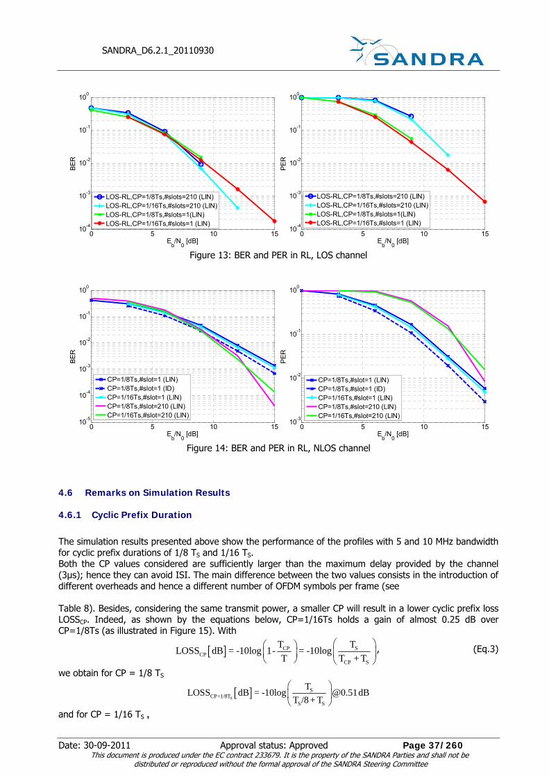
SANDRA_D6.2.1_20110930
Date: 30-09-2011 Approval status: Approved Page 37/260 This document is produced under the EC contract 233679. It is the property of the SANDRA Parties and shall not be
distributed or reproduced without the formal approval of the SANDRA Steering Committee
0 5 10 1510-4
10-3
10-2
10-1
100
Eb/N
0 [dB]
BER
LOS-RL,CP=1/8Ts,#slots=210 (LIN)LOS-RL,CP=1/16Ts,#slots=210 (LIN)LOS-RL,CP=1/8Ts,#slots=1(LIN)LOS-RL,CP=1/16Ts,#slots=1 (LIN)
0 5 10 1510-4
10-3
10-2
10-1
100
Eb/N
0 [dB]
PER
LOS-RL,CP=1/8Ts,#slots=210 (LIN)LOS-RL,CP=1/16Ts,#slots=210 (LIN)LOS-RL,CP=1/8Ts,#slots=1(LIN)LOS-RL,CP=1/16Ts,#slots=1 (LIN)
Figure 13: BER and PER in RL, LOS channel
0 5 10 1510-5
10-4
10-3
10-2
10-1
100
Eb/N
0 [dB]
BER
CP=1/8Ts,#slot=1 (LIN)CP=1/8Ts,#slot=1 (ID)CP=1/16Ts,#slot=1 (LIN)CP=1/8Ts,#slot=210 (LIN)CP=1/16Ts,#slot=210 (LIN)
0 5 10 1510-3
10-2
10-1
100
Eb/N
0 [dB]
PER
CP=1/8Ts,#slot=1 (LIN)CP=1/8Ts,#slot=1 (ID)CP=1/16Ts,#slot=1 (LIN)CP=1/8Ts,#slot=210 (LIN)CP=1/16Ts,#slot=210 (LIN)
Figure 14: BER and PER in RL, NLOS channel
4.6 Remarks on Simulation Results
4.6.1 Cyclic Prefix Duration
The simulation results presented above show the performance of the profiles with 5 and 10 MHz bandwidth for cyclic prefix durations of 1/8 TS and 1/16 TS. Both the CP values considered are sufficiently larger than the maximum delay provided by the channel (3μs); hence they can avoid ISI. The main difference between the two values consists in the introduction of different overheads and hence a different number of OFDM symbols per frame (see Table 8). Besides, considering the same transmit power, a smaller CP will result in a lower cyclic prefix loss LOSSCP. Indeed, as shown by the equations below, CP=1/16Ts holds a gain of almost 0.25 dB over CP=1/8Ts (as illustrated in Figure 15). With
[ ] CP SCP
CP S
T TLOSS dB = -10log 1- = -10logT T + T
⎛ ⎞⎛ ⎞⎜ ⎟⎜ ⎟
⎝ ⎠ ⎝ ⎠, (Eq.3)
we obtain for CP = 1/8 TS
[ ]S
SCP=1/8T
S S
TLOSS dB = -10log @0.51 dBT /8 + T
⎛ ⎞⎜ ⎟⎝ ⎠
and for CP = 1/16 TS ,

SANDRA_D6.2.1_20110930
Date: 30-09-2011 Approval status: Approved Page 38/260 This document is produced under the EC contract 233679. It is the property of the SANDRA Parties and shall not be
distributed or reproduced without the formal approval of the SANDRA Steering Committee
[ ]CP=1/16TSLOSS dB @0.26 dB .
However, more important will be the impact of the CP length on the synchronization performance.
0 2 4 6 8 10 1210-5
10-4
10-3
10-2
10-1
100
Eb/N
0 [dB]
BER
CP=1/8Ts,#slot=195 (LIN)CP=1/16Ts,#slot=195 (LIN)
Figure 15: Impact of different CP values on BER, 10 MHz profile, FL, LOS channel
4.6.2 System Bandwidth
This section compares the performance of 5 and 10 MHz profiles with LOS and NLOS channel scenarios in the FL case. The profiles generally present similar performance for both FL and RL. In the LOS channel scenario the results provided by the two scenarios are almost equivalent for all the packet sizes considered. In the NLOS channel scenario it is possible to observe a similar behavior for the smaller packet size. However, for the biggest packet sizes4 the 10 MHz bandwidth profile outperforms the 5 MHz profile. Indeed, the wider bandwidth of the system offers a better exploitation of the frequency selectivity provided by the channel. Figure 16 provides a comparison between the performance obtained with the two profiles in the FL case using CP=1/8Ts and the NLOS channel scenario. Figure 17 shows the comparison for the LOS channel scenario.
0 5 10 15 20 25 3010-6
10-5
10-4
10-3
10-2
10-1
100
Eb/N
0 [dB]
BER
10MHz,#slot=1 (LIN)10MHz,#slot=390 (LIN)10MHz,#slot=195 (LIN)5MHz,#slot=1 (LIN)5MHz,#slot=195 (LIN)
0 5 10 15 20 25 3010-5
10-4
10-3
10-2
10-1
100
Eb/N
0 [dB]
PER
10MHz,#slot=1 (LIN)10MHz,#slot=390 (LIN)10MHz,#slot=195 (LIN)5MHz,#slot=1 (LIN)5MHz,#slot=195 (LIN)
Figure 16: Comparison between 5 MHz and 10 MHz profiles, FL, NLOS channel
4 The case with BW=10MHz owns a maximum packet size bigger than the profile with BW=5MHz (390 slots against 195 slots), hence, in order to have a fair comparison the packet of 195 slots is considered also in the 10 MHz profile.

SANDRA_D6.2.1_20110930
Date: 30-09-2011 Approval status: Approved Page 39/260 This document is produced under the EC contract 233679. It is the property of the SANDRA Parties and shall not be
distributed or reproduced without the formal approval of the SANDRA Steering Committee
0 5 10 15 2010-5
10-4
10-3
10-2
10-1
100
Eb/N
0 [dB]
BER
10MHz,#slot=1 (LIN)10MHz,#slot=390 (LIN)5MHz,#slot=195 (LIN)5MHz,#slot=1 (LIN)
0 5 10 15 2010-4
10-3
10-2
10-1
100
Eb/N
0 [dB]
PER
10MHz,#slot=1 (LIN)10MHz,#slot=390 (LIN)5MHz,#slot=195 (LIN)5MHz,#slot=1 (LIN)
Figure 17: Comparison between 5 MHz and 10 MHz profiles, FL, LOS channel
4.6.3 Packet Sizes
Generally, the bigger packet sizes correspond to better performance due to a longer code. However, especially in the RL case, the differences between the results are very small. Figure 18 shows the impact of the packet size on the performance for the RL. In this case, for the NLOS channel scenario, three different packet sizes equal to 1, 45 and 102 slots are considered. All the curves are obtained with CP equal to 1/8 Ts, linear channel interpolation and the parameters provided in Table 10. The results don’t present large differences between the various cases. The blue and the red curves representing respectively the cases with 45 and 102 slots are equivalent. The smallest packet size case is outperformed by the other instances. However, its performance degradation is moderate; for a BER of 10-4 correspond to 1.4 dB (for the PER the difference is even smaller). In the FL case the effect of the packet size is similar. Though, in this case, the length of the packets has a bigger impact on the performance of the system (especially for the smallest packet size case).
0 5 10 15 20 2510
-6
10-5
10-4
10-3
10-2
10-1
100
Eb/N0 [dB]
BE
R
CP=1/8Ts,#slot=1 (LIN)CP=1/8Ts,#slot=102 (LIN)CP=1/8Ts,#slot=45 (LIN)
0 5 10 15 20 2510
-4
10-3
10-2
10-1
100
Eb/N0 [dB]
PE
R
CP=1/8Ts,#slot=1 (LIN)CP=1/8Ts,#slot=102 (LIN)CP=1/8Ts,#slot=45 (LIN)
Figure 18: Impact of the packet size on BER and PER, 5MHz profile, RL, LOS channel
Figure 19 provides a clear example of the influence of the packet sizes on the system performance in the FL. The figure shows the performance of the 5 MHz bandwidth profile in the NLOS channel scenario and compares the results obtained with packet sizes equal to 1, 10, 45, 60, 102, 150 and 195 slots. All the cases are obtained with QPSK modulation, convolutional coding with rate ½, linear channel estimation and CP=1/8 Ts. The case with packet size equal to one slot is completely outperformed by the other cases. However, the results obtained with respectively 10, 45, 60, 102 and 195 slots are almost equivalent. The reason of this result may be found in the structure of the FL frame, composed by clusters. The FL sub-channel (slot), in fact, is made by 2 non adjacent clusters. In the case of only one cluster this structure provides only limited diversity to the system, resulting in a poor performance. In the RL case, the sub-

SANDRA_D6.2.1_20110930
Date: 30-09-2011 Approval status: Approved Page 40/260 This document is produced under the EC contract 233679. It is the property of the SANDRA Parties and shall not be
distributed or reproduced without the formal approval of the SANDRA Steering Committee
channel is composed by six tiles. Hence, also in the case of 1 slot a better diversity exploitation is provide and therefore a better performance.
0 5 10 15 20 25 3010-6
10-5
10-4
10-3
10-2
10-1
100
Eb/N
0 [dB]
BER
CP=1/8Ts,#slot=1 (LIN)CP=1/8Ts,#slot=102 (LIN)CP=1/8Ts,#slot=10 (LIN)CP=1/8Ts,#slot=60 (LIN)CP=1/8Ts,#slot=150 (LIN)CP=1/8Ts,#slot=195 (LIN)CP=1/8Ts,#slot=45 (LIN)
0 5 10 15 20 25 3010-5
10-4
10-3
10-2
10-1
100
Eb/N
0 [dB]
PER
CP=1/8Ts,#slot=1 (LIN)CP=1/8Ts,#slot=102 (LIN)CP=1/8Ts,#slot=10 (LIN)CP=1/8Ts,#slot=45 (LIN)CP=1/8Ts,#slot=60 (LIN)CP=1/8Ts,#slot=150 (LIN)CP=1/8Ts,#slot=195 (LIN)
Figure 19: Impact of the packet size on BER and PER, 5MHz profile, FL, NLOS channel
4.7 Higher Modulation Schemes
In this subsection the impact of 64-QAM and 16-QAM modulations on the system performance is analyzed. The following simulation results show BER and PER obtained for FL and RL in the LOS and NLOS channel scenarios. The results are obtained with CP=1/8Ts, convolutional coding and different packet sizes.
4.7.1 FL Case
Figure 20 and Figure 21 show and compare the results obtained with QPSK, 16-QAM and 64-QAM modulations in the FL case for the 5 MHz profile. As expected, the higher modulation order curves are shifted on the right. With ideal channel estimation the 64-QAM modulation case looses almost 7 dB with respect to the QPSK case, while the 16-QAM 2.5 dB. In case of linear interpolation the 64-QAM curves present a floor due to the not perfect channel estimation. The floor is relatively high especially in the case with packet size equal to 1 slot. The 64-QAM modulation is indeed very sensitive to phase errors and a simple linear interpolation in the frequency direction in this case is not sufficient to assure good channel estimation. Figure 22 shows the results obtained in the NLOS channel scenario with linear channel interpolation. The performance is worst with respect to the LOS case; though, a similar behavior with high floor in the case with 64-QAM modulation is preserved.
0 5 10 15 20 25 3010-6
10-5
10-4
10-3
10-2
10-1
100
Eb/N
0 [dB]
BER
QPSK,1sl (LIN)QPSK,1sl (ID)64QAM,1sl (LIN)64QAM,1sl (ID)64QAM,195sl(LIN)64QAM,195sl (ID)16QAM,1sl (LIN)16QAM,1sl (ID)16QAM,195sl(LIN)
0 5 10 15 20 25 3010-5
10-4
10-3
10-2
10-1
100
Eb/N
0 [dB]
PER
QPSK,1sl(LIN)QPSK,1sl(ID)64QAM,1sl(LIN)64QAM,1sl(ID)64QAM,195sl(LIN)64QAM,195sl(ID)16QAM,1sl(LIN)16QAM,1sl(ID)16QAM,195sl(LIN)
Figure 20: Performance of 16-QAM and 64-QAM, 5MHz profile, FL, LOS channel

SANDRA_D6.2.1_20110930
Date: 30-09-2011 Approval status: Approved Page 41/260 This document is produced under the EC contract 233679. It is the property of the SANDRA Parties and shall not be
distributed or reproduced without the formal approval of the SANDRA Steering Committee
0 5 10 15 20 25 3010-6
10-5
10-4
10-3
10-2
10-1
100
Eb/N
0 [dB]
BER
64-QAM, 1slot (LIN)64-QAM, 1slot (ID)64-QAM, 195slots (LIN)64-QAM, 195slots (ID)64-QAM, 1slot (AWGN)
0 5 10 15 20 25 3010-3
10-2
10-1
100
Eb/N
0 [dB]
PER
64-QAM, 1slot (LIN)64-QAM, 1slot (ID)64-QAM, 195slots (LIN)64-QAM, 195slots (ID)64-QAM, 1slot (AWGN)
Figure 21: Performance of 64-QAM modulation in FL with AWGN and SANDRA LOS channel, 5 MHz profile
0 5 10 15 20 25 3010-6
10-5
10-4
10-3
10-2
10-1
100
Eb/N
0 [dB]
BER
QPSK,1sl(LIN)16-QAM,1sl(LIN)64-QAM,1sl(LIN)
0 5 10 15 20 25 3010-5
10-4
10-3
10-2
10-1
100
Eb/N
0 [dB]
PER
QPSK,1sl(LIN)16-QAM,1sl(LIN)64-QAM,1sl(LIN)
Figure 22: Performance of different modulation schemes in FL with NLOS channel, 5 MHz profile
4.7.2 RL Case
Figure 23 provides the performance of the RL in the LOS channel scenario with 64-QAM and 16-QAM modulations in comparison with QPSK modulation. Similarly to the FL case, in correspondence of ideal channel estimation the 64-QAM case presents a loose of almost 7-8 dB with respect to the QPSK case. Though, differently from the previously-evaluated FL case, the linear channel estimation cases don’t present any floor. The obtained result can be explained analyzing the structure of the RL frame. In frame based on tiles (Figure 5), the pilot sub-carriers are close (the pilot separation is 3 sub-carriers in frequency direction and 2 in time direction) which help the channel estimator to properly track the channel behavior. The FL frame presents pilot subcarriers more distant, which provides a less accurate tracking of the channel. Focusing on the RL and on the 64-QAM modulation case, Figure 24 shows the results obtained with the LOS scenario without Doppler effect. The black curve has been obtained assuming no Doppler spread and shift and linear channel estimation. The elimination of the Doppler effects reduces the selectivity of the channel reducing also the benefits introduced. The black curve presents indeed worst performance with respect to the magenta curve (same parameters but Doppler). In the considered case, in fact, no Inter-Carrier Interference (ICI) is present, since the subcarrier spacing of almost 10 kHz is far bigger of the

SANDRA_D6.2.1_20110930
Date: 30-09-2011 Approval status: Approved Page 42/260 This document is produced under the EC contract 233679. It is the property of the SANDRA Parties and shall not be
distributed or reproduced without the formal approval of the SANDRA Steering Committee
impact of the Doppler. Hence, Doppler effect in this case only brings a moderate increasing of the channel selectivity which brings a benefit on the performance of the OFDM system.
0 5 10 15 20 25 3010-6
10-5
10-4
10-3
10-2
10-1
100
Eb/N
0 [dB]
BER
QPSK,1sl(LIN)QPSK,1sl(ID)64-QAM,1sl(LIN)64-QAM,1sl(ID)64-QAM,102sl(LIN)16-QAM,1sl(LIN)16-QAM,1sl(ID)16-QAM,102sl(LIN)
0 5 10 15 20 25 3010-5
10-4
10-3
10-2
10-1
100
Eb/N
0 [dB]
PER
QPSK,1sl(LIN)QPSK,1sl(ID)64-QAM,1sl(LIN)64-QAM,1sl(ID)64-QAM,102sl(LIN)16-QAM,1sl(LIN)16-QAM,1sl(ID)16-QAM,102sl(LIN)
Figure 23: Performance of 16-QAM and 64-QAM modulations in RL, LOS channel, 5MHz profile
0 5 10 15 20 2510
-5
10-4
10-3
10-2
10-1
100
Eb/N0 [dB]
BE
R
64-QAM,1slot (LIN)64-QAM,1slot (ID)64-QAM,1sl,(LIN) NO-DOP
Figure 24: Evaluation of Doppler effect on 64-QAM performance in RL with LOS channel, 5 MHz profile
The evaluation of higher modulation orders in the NLOS channel scenario is showed in Figure 25 for packet length 1 slot and linear channel interpolation. In this case, the 16-QAM curve is 2.5 dB shifted on the right with respect to QPSK, while 64-QAM is 5 dB further on the right.
0 5 10 15 20 25 3010-6
10-5
10-4
10-3
10-2
10-1
100
Eb/N
0 [dB]
BER
QPSK,1sl(LIN)16-QAM,1sl(LIN)64-QAM,1sl(LIN)
0 5 10 15 20 25 3010-5
10-4
10-3
10-2
10-1
100
Eb/N
0 [dB]
PER
QPSK,1sl(LIN)16-QAM,1sl(LIN)64-QAM,1sl(LIN)
Figure 25: Impact of different modulations in RL, NLOS channel, 5MHz profile

SANDRA_D6.2.1_20110930
Date: 30-09-2011 Approval status: Approved Page 43/260 This document is produced under the EC contract 233679. It is the property of the SANDRA Parties and shall not be
distributed or reproduced without the formal approval of the SANDRA Steering Committee
4.8 Impact of Synchronisation Errors on BER
In the previous sections we evaluated the performance of the system with perfect synchronization. Instead of implementing the synchronisation algorithm in the JAVA simulator, a simplified block that introduces synchronisation errors has been added. In order to achieve realistic results, we modeled synchronization offsets according to values obtained by the synchronisation algorithm presented in Chapter 5. This section shows the impact of the modeled timing and frequency errors on the performance of the system. Later in Section 6.3, an overall performance of a system with implemented synchronisation and channel estimation algorithms will be presented. The results presented in Sect. 5.3 are similar to those presented in this section and thus, verify the simulation model applied. Regarding the synchronisation performance presented in Chapter 5, we considered the 10 MHz profile in the LOS channel scenario. Moreover, we used packets long 1slot, CP=1/8Ts, QPSK modulation and linear channel interpolation. The timing and the frequency offsets were empirically modeled with a Gaussian distribution which approximates the distributions of the offset values obtained from the synchronisation simulations performed according to Chapter 5. Figure 26 shows on the left hand the Gaussian approximation (red line) for SNR=10 dB having a mean µ=2ns and a variance σ=2.21. On the right hand, it shows the performance of the system using the timing offset model in comparison with the results obtained with real offset values. The model results, represented in green, overlap the curve obtained with realistic time offsets, proving the efficiency of the model. However, the synchronization algorithms perform very well and the impact of the offsets is negligible.
-60 -40 -20 0 20 40 600
0.02
0.04
0.06
0.08
0.1
0.12
0.14
0.16
0.18
0.2
ns
Real pdfGaussian approx.
0 2 4 6 8 10 12 14 16 18 2010-7
10-6
10-5
10-4
10-3
10-2
10-1
100
Eb/N0
BE
R
time off 0%time off VARIABLEtime offset gauss
Figure 26: Modeling of the timing offset for SNR=10dB (left) and performance results (right)
Figure 27 shows the results obtained for the FL. Frequency and timing offsets are simulated separately. Figure 28 provides the performance of the RL. In this case, also the ranging effects are accounted and in particular 4 different scenarios are considered. Besides the case with only one user (represented in blue), different numbers of multiple users are evaluated. The users utilize the same ranging code, hence, the probability of collision increases with the number of users. However, up to 7 interferes the performance of the system doesn’t degrades. In both FL and RL, the impact of the synchronization offsets is negligible, therefore the assumption made in the previous simulations holds.
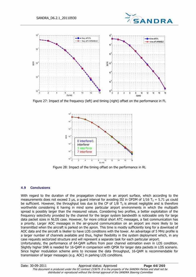
SANDRA_D6.2.1_20110930
Date: 30-09-2011 Approval status: Approved Page 44/260 This document is produced under the EC contract 233679. It is the property of the SANDRA Parties and shall not be
distributed or reproduced without the formal approval of the SANDRA Steering Committee
0 2 4 6 8 10 12 1410
-4
10-3
10-2
10-1
100
Eb/N0
BE
R
freq off 0%freq off VARIABLE
0 2 4 6 8 10 12 14 16 1810-6
10-5
10-4
10-3
10-2
10-1
100
Eb/N0
BE
R
time off 0%time off VARIABLE
Figure 27: Impact of the frequency (left) and timing (right) offset on the performance in FL
0 2 4 6 8 10 12 14 16 1810-6
10-5
10-4
10-3
10-2
10-1
100
Eb N0
BE
R
Figure 28: Impact of the timing offset on the performance in RL
4.9 Conclusions
With regard to the duration of the propagation channel in an airport surface, which according to the measurements does not exceed 3 µs, a guard interval for avoiding ISI in OFDM of 1/16 TS = 5.71 µs could be sufficient. However, the throughput loss due to the CP of 1/8 TS is almost negligible and is therefore worthwhile considering it having in mind some particular airport environments in which the multipath spread is possibly larger than the measured values. Considering two profiles, a better exploitation of the frequency selectivity provided by the channel for the larger system bandwidth is noticeable only for large data packet sizes in NLOS case. However, for more critical short ATC messages, a fast communication has a priority. Larger AOC messages in the air-ground communication on an airport are more likely to be transmitted when the aircraft is parked on the apron. This time is mostly sufficiently long for a download of AOC data and the aircraft is likelier to have LOS conditions with the tower. An advantage of 5 MHz profile is a larger number of channels available and thus, higher flexibility in the system deployment which, in any case requests sectorized structure and will represent a separate task for each particular airport. Unfortunately, the performance of 64-QAM suffers from poor channel estimation even in LOS condition. Slightly higher SNR is needed for 16-QAM in comparison with QPSK for larger data packets in LOS scenario. Since higher modulation scheme aims to increase the data throughput, 16-QAM is recommendable for transmission of larger messages (e.g. AOC) in parking LOS conditions.
0 interferer1 interferer 3 interferer 7 interferer

SANDRA_D6.2.1_20110930
Date: 30-09-2011 Approval status: Approved Page 45/260 This document is produced under the EC contract 233679. It is the property of the SANDRA Parties and shall not be
distributed or reproduced without the formal approval of the SANDRA Steering Committee
The performance of the system with 5 and 10 MHz bandwidth, with different cyclic prefix length, in different channel condition (LOS and NLOS) and for different modulation schemes is also listed in tabular form in Appendix A of this document. Whereas this performance analysis assumed perfect synchronisation and simple channel estimation, the following chapters are in particularly dedicated to these topics. Furthermore, a possible performance improvement by utilizing a multiple antenna scheme is also separately investigated in Chapter 7.

SANDRA_D6.2.1_20110930
Date: 30-09-2011 Approval status: Approved Page 46/260 This document is produced under the EC contract 233679. It is the property of the SANDRA Parties and shall not be
distributed or reproduced without the formal approval of the SANDRA Steering Committee
5 Synchronization and Ranging This chapter evaluates the synchronization algorithms applied for the PHY layer of AeroMACS system within SANDRA project. The fixed system parameters of the investigated AeroMACS profile are summarized in Table 7. The analysis of the synchronisation and ranging algorithm is performed for the system profile of 10 MHz and the corresponding (variable) parameter can be taken from Table 8. Section 5.3 illustrates the synchronization algorithms for the forward link while synchronization in the reverse link is investigated in Section 5.4. The major theoretical results are highlighted in the attached Appendices XX. The performance of the synchronization algorithms is computed by simulation and compared with theoretical analysis (when possible).
5.1 FL Synchronization
In FL, each MS receives the broadcast signal transmitted by the BS and performs the following operations:
1. it checks whether a training symbol is present or not in the received sample stream;
2. after the training symbol has been detected, it computes a timing estimate to identify the
beginning of the FL frame;
3. it computes an estimate of the Fractional Carrier Frequency Offset (FCFO);
4. it estimates the Integer Carrier Frequency Offset (ICFO) and identifies the BS on the basis of the
transmitted training symbol;
5. it performs channel estimation and equalization;
6. In the sequel, we will discuss all the aforementioned operations.
5.1.1 Detection of the Training Symbol The first task that MS must accomplish during the FL synchronization phase is the detection of the training symbol within the stream of received samples. As specified in [WiM01], the training symbol is placed at the beginning of each frame (training preamble) and contains N = 1024 subcarriers with indices
0,1, , 1n N= −K . Out of all available 1024 subcarriers, only a subset of 284 subcarriers are actually modulated by a Pseudo-Noise (PN) BPSK sequence. This sequence is selected among 114 possible choices and univocally identifies the transmitting BS. The modulated subcarriers are separated by a couple of unmodulated (null) subcarriers and there are 86 guard band subcarriers on each side of the signal spectrum. The indices of the modulated subcarriers during the frame preamble are given by
im = η0 + 3mN
−142 ≤ m ≤ 141 (Eq.4)
where η0 ∈{0,1,2} is an unknown parameter that designates the preamble carrier-set for identification of
the cell sector, while the notation n N denotes the modulo-n operation reducing n to the interval
[0, N −1] . Figure 29 illustrates the basic structure of the frame preamble assuming thatη0 = 0 . As it is seen, we have a first set of modulated subcarriers with indices running from 0 to 423 and belonging to the portion of spectrum placed at the right-hand side of the carrier frequency, while a second set of subcarriers with indices running from 598 to 1021 is placed at the left-hand side of the carrier frequency.

SANDRA_D6.2.1_20110930
Date: 30-09-2011 Approval status: Approved Page 47/260 This document is produced under the EC contract 233679. It is the property of the SANDRA Parties and shall not be
distributed or reproduced without the formal approval of the SANDRA Steering Committee
0 3 6 423 598 601 604 1021 Figure 29: Basic structure of the FL frame preamble
The training preamble is preceded by a CP containing Ng = 128 samples. The complex envelope of the
transmitted signal is thus given by
sp (t) =AN
apm=−142
141
∑ (m)e j2π (η0 +3m )t /Tu − Tg ≤ t ≤ Tu (Eq.5)
where { ( 142), ( 141), , (141)}p p p pa a a a= − − … is the sequence of pilot symbols belonging to the p-th
preamble (with 0,1, ,113p = K and ap (m) = ±1 ), while A = 2 2 accounts for the power boosting
applied to the pilot tones. It is worth observing that the integer η0 is univocally determined by the preamble index p as specified in [WiM01]. The samples of sp (t) at times tk = kTu / N take the form
sp (k) =AN
apm=−142
141
∑ (m)e j 2π k (η0 +3m)/ N − Ng ≤ k ≤ N −1. (Eq.6)
Expression (Eq.5) indicates that sp (t) is the product of a periodic signal with period Tu / 3 multiplied by a
complex exponential e j 2πη0 t /Tu . Unfortunately, such periodicity does not hold true for the corresponding samples sp (k) since N is not a multiple of three. However, we expect that samples corresponding to the
training preamble taken at a distance of Nc = N / 3⎢⎣ ⎥⎦ = 341 are highly correlated in practice.
We denote by fΔ the CFO normalized by the subcarrier spacing. The samples received at the MS and corresponding to the training preamble are thus given by
r(k) =AN
e j 2π ( fΔ +η0 )k / N ap (m)H (im )m=−142
141
∑ e j 6πmk / N + w(k) (Eq.7)
with im being defined as in (Eq.4). The quantities w(k) account for thermal noise and are modeled as
statistically independent and complex-valued Gaussian random variables with zero-mean and variance σw2 ,
while H (im ) is the channel frequency response over the im th subcarrier. Denoting by
[ (0), (1), , ( 1)]h h h L= −h K the Channel Impulse Response (CIR), we have
1
2 /
0( ) ( ) 0 1
Lj n NH n h e n Nπ
−−
=
= ≤ ≤ −∑ l
l
l (Eq.8)
where the energy of h is normalized such that
{ }2E ( ) 1H n = (Eq.9)
for 0,1, , 1n N= −K . To proceed further, we define the Nc − lag correlation of r(k) as
Rr (Nc ) = E{r(k + Nc )r∗(k)} . (Eq.10) Then, substituting (Eq.7) into (Eq.10) and modeling the pilot symbols as statistically independent random variables, we see that during the training preamble it is
Rr (Nc ) =A2
Ne j 2π ( fΔ +η0 )Nc / N e j 6πmNc / N
m=−142
141
∑ (Eq.11)

SANDRA_D6.2.1_20110930
Date: 30-09-2011 Approval status: Approved Page 48/260 This document is produced under the EC contract 233679. It is the property of the SANDRA Parties and shall not be
distributed or reproduced without the formal approval of the SANDRA Steering Committee
or, equivalently, Rr (Nc ) = 1.95 × e j 2π ( fΔ +η0 )Nc / N × e jπ / N . (Eq.12) On the other hand, the samples received at the MS and belonging to an OFDM data symbol are expressed by r(k) = e j2π fΔ k / N sR (k) + w(k) (Eq.13)
where sR (k) is the useful component of the received signal, which takes the form
sR (k) =1N
c(n)H (n)e j 2πnk / N
n=−420
420
∑ . (Eq.14)
In the above expression, the information symbols {c(n)} are modeled as statistically independent random
variables with zero mean and energy { }22 E ( )C c n= . Substituting (Eq.14) into (Eq.10) provides the
Nc − lag correlation corresponding to an OFDM data symbol in the form
Rr (Nc ) =C2
Ne j 2π fΔNc / N e j 2πnNc / N
n=−420
420
∑ (Eq.15)
which can also be rewritten as Rr (Nc ) = 2.1×10⁻⁴ × C2e
j 2π fΔNc / N . (Eq.16)
Comparing the results (Eq.12) and (Eq.16) reveals that Rr (Nc ) is significantly larger during the training
preamble than during an OFDM data symbol. This suggests that Rr (Nc ) can provide useful information
as to whether a training preamble is present or not in the received samples {r(k)} . Unfortunately, the
quantity Rr (Nc ) is not available at the receiver due to the presence of the statistical expectation in the
right-hand-side of (Eq.10). To overcome this difficulty, we replace Rr (Nc ) by the sample correlation function evaluated over an integration window spanning 2Nc samples. This function is defined as
C(d) =1
2Nc
r∗k=0
2 Nc −1
∑ (d + k)r(d + k + Nc ) (Eq.17)
where d is a time index which slides along in time as the receiver searches for the training preamble. The quantity C(d) is then normalized by an estimate of the received energy over the integration window,
which is obtained as
P(d) =1
2Nc
r(d + k) 2
k=0
2 Nc −1
∑ . (Eq.18)
This provides a metric
M (d) =C(d)
max{P(d),P(d + Nc )} (Eq.19)
which is virtually independent of the instantaneous received power. In order to reduce the implementation complexity, the quantities C(d) and P(d) can be iteratively computed as
C(d +1) = C(d) +1
2Nc
r∗(d + 2Nc )r(d + 3Nc ) − r∗(d)r(d + Nc )⎡⎣ ⎤⎦ (Eq.20)
P(d +1) = P(d) +1
2Nc
r(d + 2Nc ) 2− r(d) 2⎡
⎣⎤⎦ (Eq.21)
for 0,1,2,d = K , with
C(0) =1
2Nc
r∗k=0
2 Nc −1
∑ (k)r(k + Nc ) (Eq.22)

SANDRA_D6.2.1_20110930
Date: 30-09-2011 Approval status: Approved Page 49/260 This document is produced under the EC contract 233679. It is the property of the SANDRA Parties and shall not be
distributed or reproduced without the formal approval of the SANDRA Steering Committee
P(0) =1
2Nc
r(k) 2
k=0
2 Nc −1
∑ . (Eq.23)
Substituting (Eq.7) into (Eq.18) and computing the expectation yields
E{P(d)} =284 ⋅ A2
N+ σw
2 = 2.22 + σw2 . (Eq.24)
Bearing in mind (Eq.12) and (Eq.24), from (Eq.19) we see that for d = 0 (which corresponds to the peak of the timing metric) we have
E{M (0)} ≈1.95
2.22 + σw2 (Eq.25)
meaning that, at relatively large SNR values, the peak of M (d) is expected to be in the order of 0.85. This
conjecture is validated by the experimental results shown in Figure 30, illustrating the metric M (d) as a function of d. In this experiment, a silent period where nothing is transmitted is followed by a training preamble plus four OFDM data symbols. The mobile speed is fixed to 30 m/s while the SNR is set 10 dB. Throughout this report, we define the SNR as the ratio between the average power of the received signal
component { }22 E ( )s Rs kσ = during an OFDM data symbol and the average noise power σw2 . The
propagation channel is the NLOS channel model discussed in Section 4.2.1.2, which is characterized by 12 multipath components with a specified power delay profile. A new channel snapshot is generated at the frame beginning and the path gains are varied during the FL subframe according to the mobile speed v.
1.0
0.8
0.6
0.4
0.2
0.0
met
ric M
(d)
300025002000150010005000
d
SNR = 10 dBv = 30 m/s
Figure 30: Metric M (d) obtained with SNR = 10 dB
As it is seen, the metric M (d) has a peak in the neighborhood of the training preamble and exhibits a plateau whose duration is approximately equal to the CP length. A synch flag indicating the presence of the training symbol is thus obtained by comparing M (d) with a suitable threshold λ0 . More precisely, assume
that M (d0 −1) < λ0 and M (d0 ) > λ0 . Then, frame detection is declared at d = d0 , after which the receiver starts a synchronization procedure to acquire timing and frequency information as illustrated later. The threshold λ0 must be designed so as to achieve a reasonable tradeoff between the false alarm
probability Pfa (i.e., the probability of detecting a frame preamble when it is actually absent) and the
misdetection probability Pmd (i.e., the probability of not detecting a preamble when it is actually present).
Clearly, increasing λ0 reduces Pfa , but degrades the detection capability. A common approach for the

SANDRA_D6.2.1_20110930
Date: 30-09-2011 Approval status: Approved Page 50/260 This document is produced under the EC contract 233679. It is the property of the SANDRA Parties and shall not be
distributed or reproduced without the formal approval of the SANDRA Steering Committee
threshold design is based on the Neyman-Pearson criterion, according to which λ0 is selected so as to
achieve a target value of Pfa . In Appendix B1 it is shown that the false alarm probability is approximately
given by Pfa = exp(−2λ0
2Nc ) (Eq.26)
and turns out to be independent of the SNR level. Solving (Eq.26) with respect to λ0 yields
λ0 =ln(1 / Pfa )
2Nc
(Eq.27)
which can be used to select the threshold that corresponds to a specified false alarm probability. In Figure 31 we report numerical measurements illustrating Pfa and Pmd as a function of the threshold λ0 .
The SNR is either 0 or 10 dB. As is seen, Pfa is virtually independent of the SNR and attains the theoretical
analysis presented in (Eq.26). Vice versa, Pmd rapidly decreases as the SNR grows large. In order to
illustrate how the results of Figure 31 can be used, assume that we want to achieve a Pfa value of 10−10 ,
which corresponds to λ0 = 0.185 in (Eq.27). In such a case, for an SNR of 0 dB we see from Figure 31
that Pmd is approximately10−4 . This means that the probability of mis-detecting a training preamble during
an observation window spanning NF frames is approximately given by 10−4 NF and becomes vanishingly
small as NF increases. In other words, in case the training preamble is missed during a specific forward link frame, it will be detected with high probability in one of the subsequent frames.
10 -5
10-4
10 -3
10-2
10 -1
100
1.00.80.60.40.20.0
threshold, λ0
theory
Ng=128v = 30 m/s
SNR = 0dB SNR = 10dB
Pfa
Pmd
Figure 31: Pfa and Pmd as a function of λ0 with SNR = 0 or 10 dB
5.1.2 Timing Estimation
Assume that the metric M (d) overcomes the threshold λ0 at d = d0 . Then, the receiver starts a timing synchronization procedure whose goal is to identify the beginning of each OFDMA block so as to find the correct position of the DFT window. Since the CFO is still unknown in this phase, it is desirable that the timing recovery scheme be robust against possibly large frequency offsets. Unfortunately, M (d) cannot provide reliable timing information since the plateau region shown in Figure 30 reduces its localization capability. A popular approach for timing estimation in multicarrier systems relies on the autocorrelation

SANDRA_D6.2.1_20110930
Date: 30-09-2011 Approval status: Approved Page 51/260 This document is produced under the EC contract 233679. It is the property of the SANDRA Parties and shall not be
distributed or reproduced without the formal approval of the SANDRA Steering Committee
properties that the cyclic prefix induces on the time domain samples [KE_01], [BE_97]. In practice, the following N − lag autocorrelation function is used as timing metric
γ (d) = r(k=0
Ng −1
∑ d + k + N )r∗(d + k) d0 +1≤ d ≤ d0 + NT (Eq.28)
where NT = N + Ng is the block length (including the CP) expressed in sampling intervals. In practice,
γ (d) is recursively computed as
γ (d +1) = γ (d) + r(d + Ng + N )r∗(d + Ng ) − r(d + N )r∗(d) (Eq.29)
for 0 01, 2,d d d= + + K , with γ (d0 ) obtained as in (Eq.28). Since the CP is just a duplication of the last
Ng samples of the OFDM block, we expect that γ (d) exhibits a peak whenever the samples r(d + k)
with 0 ≤ k ≤ Ng −1 belong to the CP. This intuition is confirmed by the experimental results of Figure 32,
where γ (d) is shown as a function of the time index d for Ng = 128 and SNR = 10 dB. The CIR is
compliant with that in Section 4.2.1. As we can see, γ (d) is characterized by a sharp peak positioned at
the beginning of the received OFDMA block. Since the peak does not exhibit any plateau region, we expect that timing information can be achieved from γ (d) without any ambiguity.
150
100
50
0
timin
g m
etric
140012001000800600
time index, d
Ng=128SNR = 10 dBv = 30 m/s
Figure 32: Timing metric γ (d ) as obtained with SNR = 10 dB
It should be observed that, in applications where the CP length Ng is relatively small, accurate timing
recovery may be difficult to be gained as a consequence of the short integration window employed in (Eq.28). A possible remedy to this drawback consists of averaging γ (d) over a specified number M B of OFDM block. This produces the following modified metric
γ (d) = γ (d + mNT )m=0
M B −1
∑ (Eq.30)
in which γ (d) is still computed as in (Eq.28). The timing estimate is eventually found by locating the
global maximum of γ (d) over a time interval I = [d0 +1,d0 + NT ] , i.e.,
{ }ˆ arg max ( )d I
d dγ∈
= . (Eq.31)

SANDRA_D6.2.1_20110930
Date: 30-09-2011 Approval status: Approved Page 52/260 This document is produced under the EC contract 233679. It is the property of the SANDRA Parties and shall not be
distributed or reproduced without the formal approval of the SANDRA Steering Committee
Numerical results illustrating the probability density function (pdf) of d as obtained with Ng = 128 and
ν = 0 m/s are illustrated in Figure 33: and Figure 34 for M B = 1 and 4, respectively. Again, we let
SNR = 10 dB. In these experiments, the value d = 0 corresponds to the first sample of the CP and
represents the correct timing instant. As expected, the pdf of d becomes narrower as M B increases due to the improved accuracy of the corresponding timing estimate. While in an AWGN channel the mean of the metric peak is exactly placed at the start of the OFDM symbol (i.e., at d = 0 ), in a multipath channel it is delayed by some samples as a consequence of the channel dispersion. This is confirmed by the fact that
E{d} > 0 in Figure 33: and Figure 34. Similar conclusions apply when the mobile speed is set to 30 m/s, as it is witnessed by the results shown in Figure 35 and Figure 36.
0.35
0.30
0.25
0.20
0.15
0.10
0.05
0.00
pdf o
f tim
ing
estim
ate
-30 -20 -10 0 10 20 30
time index, d
Ng=128SNR = 10 dBMB = 1v = 0 m/s
Figure 33: Probability density function of the timing estimate with SNR = 10 dB, M B = 1 and ν = 0 m/s
0.35
0.30
0.25
0.20
0.15
0.10
0.05
0.00
pdf o
f tim
ing
estim
ate
-30 -20 -10 0 10 20 30
time index, d
Ng=128SNR = 10 dBMB = 4v = 0 m/s
Figure 34: Probability density function of the timing estimate with SNR = 10 dB, M B = 4 and ν = 0 m/s

SANDRA_D6.2.1_20110930
Date: 30-09-2011 Approval status: Approved Page 53/260 This document is produced under the EC contract 233679. It is the property of the SANDRA Parties and shall not be
distributed or reproduced without the formal approval of the SANDRA Steering Committee
0.35
0.30
0.25
0.20
0.15
0.10
0.05
0.00
pdf o
f tim
ing
estim
ate
-30 -20 -10 0 10 20 30
time index, d
Ng=128SNR = 10 dBMB = 1v = 30 m/s
Figure 35: Probability density function of the timing estimate with SNR = 10 dB, M B = 1 and ν = 30 m/s
0.35
0.30
0.25
0.20
0.15
0.10
0.05
0.00
pdf o
f tim
ing
estim
ate
-30 -20 -10 0 10 20 30
time index, d
Ng=128SNR = 10 dBMB = 4v = 30 m/s
Figure 36: Probability density function of the timing estimate with SNR = 10 dB, M B = 4 and ν = 30 m/s
It is known that IBI will be present during the payload section of the frame whenever the timing estimate
d lies outside the interval Jd = [L −1, Ng ] , where L is the CIR length expressed in sampling intervals.
Intuitively speaking, the probability of occurrence of IBI can be reduced by shifting the expected value of the timing estimate toward the middle point of Jd , which is given by (L −1+ Ng ) / 2 . This leads to the
following refined timing estimate
( )ˆ ˆ ˆE{ } ( 1 ) / 2fgd d d L N= − + − + . (Eq.32)
Extensive simulations indicate that E{d} equals the mean delay associated to the channel response. This
parameter is generally unknown at the receiver, but can roughly be approximated by (L −1) / 2 . Using this result into (Eq.32), yields the final timing estimate in the form
d ( f ) = d + Ng / 2 . (Eq.33)
The performance of the timing estimator is assessed in terms of probability of making a timing error, say
Pf . An error event is declared to occur whenever the estimate d ( f ) gives rise to IBI at the DFT output,

SANDRA_D6.2.1_20110930
Date: 30-09-2011 Approval status: Approved Page 54/260 This document is produced under the EC contract 233679. It is the property of the SANDRA Parties and shall not be
distributed or reproduced without the formal approval of the SANDRA Steering Committee
which amounts to saying that d ( f ) does not belong to Jd . Figure 37 illustrates Pf as a function of the
number M B of OFDMA blocks employed to get γ (d) in (Eq.30). The SNR is either 0 or 10 dB, while
Ng = 128 . As it is seen, with an SNR of 10 dB we can achieve a Pf value of approximately 10−5 by
letting M B = 2 , while 16 OFDMA blocks are required when SNR = 0 dB.
10-5
10-4
10-3
10-2
10 -1
prob
abili
ty o
f a ti
min
g er
ror,
Pf
161412108642
number of blocks, M B
Ng=128v = 30 m/s
SNR=0dB SNR=10dB
Figure 37: Probability of a timing error vs. the number of OFDMA blocks with Ng = 128 and SNR = 0 or 10
dB
5.1.3 Estimation of the Fractional Frequency Offset
The presence of a carrier frequency offset produces a shift of the received signal in the frequency domain. In multicarrier applications, it is expedient to decompose the frequency error fΔ into an integer part (ICFO), which is multiple of the subcarrier spacing Δf = 1 / Tu , plus a remaining fractional part (FCFO),
less than Δf / 2 in magnitude. This amounts to putting
f ε μΔ = + (Eq.34)
where μ is integer-valued and represents the ICFO, while ε is the FCFO belonging to the interval
(−0.5,+0.5) . If not properly compensated, the former results into a shift of the subcarrier indices at the DFT output, while the latter produces ICI and Multiple Access Interference (MAI) due to a loss of orthogonality among subcarriers. The frequency estimation algorithm provides an estimate of fΔ in the form
ˆ ˆ ˆf ε μΔ = + (Eq.35)
where ε and μ are the estimates of ε and μ , respectively. Here, we concentrate on the acquisition of ε , while the problem of estimating the integer offset μ is addressed later. Conventional methods for estimating the fractional offset operate in the time domain and measure the phase shift between the repetitive parts of a dedicated pilot block. A representative set of the results obtained in this area can be found in [SCH_03], [SH_04] and [MO_99]. Here, we follow the approach outlined in [BE_97], wherein the frequency error is retrieved by exploiting the redundancy associated to the
cyclic prefix. We begin by considering the timing metric γ (d) evaluated at the optimum time instant d
given in (Eq.31). Substituting (Eq.28) into (Eq.30) and letting dk ,m = d + k + mNT for notational

SANDRA_D6.2.1_20110930
Date: 30-09-2011 Approval status: Approved Page 55/260 This document is produced under the EC contract 233679. It is the property of the SANDRA Parties and shall not be
distributed or reproduced without the formal approval of the SANDRA Steering Committee
conciseness, we obtain
γ (d) = r(dk ,m + N )r∗(dk ,m )k=0
Ng −1
∑m=0
M B −1
∑ (Eq.36)
where r(k) are the received samples, which can be expressed as
r(k) = sR (k)e j 2π fΔ k / N + w(k) . (Eq.37)
In the above equation, w(k) is white Gaussian noise with zero-mean and variance σw2 , while sR (k) is the
useful signal component given in (Eq.14). To proceed further, we put (Eq.37)
into the equivalent form 2 /( ) [ ( ) ( )]j f k N
Rr k e s k w kπ Δ= + % (Eq.38)
where %w(k) = w(k)e− j 2π fΔ k / N has the same statistics of w(k) . Then, we assume that the samples
,ˆ{ ( ); 0,1, , 1}k m gr d k N= −K belong to the CP of the m-th OFDMA block. Such a situation occurs with unit
probability in the absence of thermal noise and for transmissions over an AWGN channel. In the presence of thermal noise and multipath propagation, it holds true with high probability provided that the timing
estimate d is sufficiently accurate. Hence, neglecting the contribution of IBI for simplicity, we have
,ˆ2 /
, , ,ˆ ˆ ˆ( ) [ ( ) ( )]k mj f d N
k m R k m k mr d e s d w dπ Δ= + % (Eq.39)
,ˆ2 ( ) /
, , ,ˆ ˆ ˆ( ) [ ( ) ( )]k mj f d N N
k m R k m k mr d N e s d w d Nπ Δ ++ = + +% (Eq.40)
which, combined with (Eq.36), yields
γ (d) = M BNgσ s2e j 2π fΔ (1+η) (Eq.41)
where
σ s2 =
1M BNg
sR (dk ,m )2
k=0
Ng −1
∑m=0
M B −1
∑ (Eq.42)
is the received signal energy, and
2
11
, , , , , ,0 0
1
ˆ ˆ ˆ ˆ ˆ ˆ[ ( ) ( ) ( ) ( ) ( ) ( )]gB
B g s
NM
k m k m k m k m k m k mm k
M N
s d w d s d w d N w d w d N
ησ−−
∗ ∗ ∗
= =
= ×
+ + + +∑ ∑ % % % %
(Eq.43)
is a disturbance term. Recalling that fΔ = ε + μ with μ being integer valued, from (Eq.41) we see that an estimate of the FCFO can be computed as
{ }1 ˆˆ arg ( )2
dε γπ
= (Eq.44)
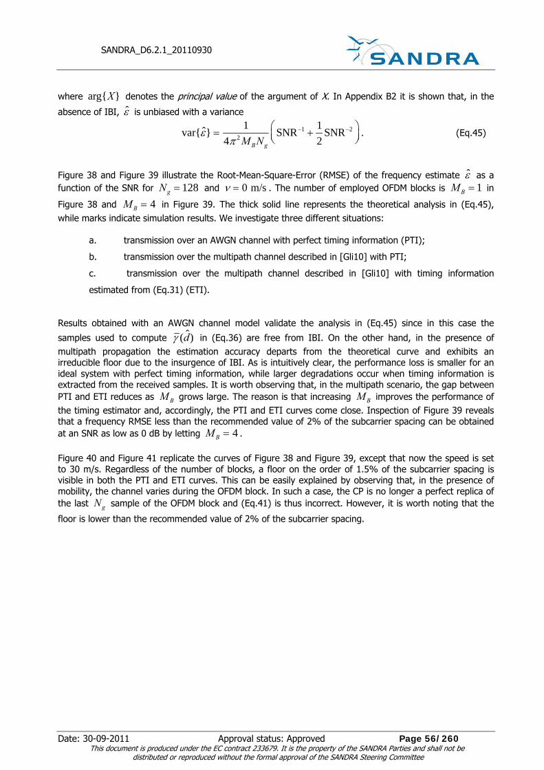
SANDRA_D6.2.1_20110930
Date: 30-09-2011 Approval status: Approved Page 56/260 This document is produced under the EC contract 233679. It is the property of the SANDRA Parties and shall not be
distributed or reproduced without the formal approval of the SANDRA Steering Committee
where arg{X} denotes the principal value of the argument of X. In Appendix B2 it is shown that, in the
absence of IBI, ε is unbiased with a variance
var{ε} =1
4π 2M BNg
SNR−1 +12
SNR−2⎛⎝⎜
⎞⎠⎟
. (Eq.45)
Figure 38 and Figure 39 illustrate the Root-Mean-Square-Error (RMSE) of the frequency estimate ε as a function of the SNR for Ng = 128 and ν = 0 m/s . The number of employed OFDM blocks is M B = 1 in
Figure 38 and M B = 4 in Figure 39. The thick solid line represents the theoretical analysis in (Eq.45), while marks indicate simulation results. We investigate three different situations:
a. transmission over an AWGN channel with perfect timing information (PTI);
b. transmission over the multipath channel described in [Gli10] with PTI;
c. transmission over the multipath channel described in [Gli10] with timing information
estimated from (Eq.31) (ETI).
Results obtained with an AWGN channel model validate the analysis in (Eq.45) since in this case the
samples used to compute γ (d) in (Eq.36) are free from IBI. On the other hand, in the presence of multipath propagation the estimation accuracy departs from the theoretical curve and exhibits an irreducible floor due to the insurgence of IBI. As is intuitively clear, the performance loss is smaller for an ideal system with perfect timing information, while larger degradations occur when timing information is extracted from the received samples. It is worth observing that, in the multipath scenario, the gap between PTI and ETI reduces as M B grows large. The reason is that increasing M B improves the performance of the timing estimator and, accordingly, the PTI and ETI curves come close. Inspection of Figure 39 reveals that a frequency RMSE less than the recommended value of 2% of the subcarrier spacing can be obtained at an SNR as low as 0 dB by letting M B = 4 . Figure 40 and Figure 41 replicate the curves of Figure 38 and Figure 39, except that now the speed is set to 30 m/s. Regardless of the number of blocks, a floor on the order of 1.5% of the subcarrier spacing is visible in both the PTI and ETI curves. This can be easily explained by observing that, in the presence of mobility, the channel varies during the OFDM block. In such a case, the CP is no longer a perfect replica of the last Ng sample of the OFDM block and (Eq.41) is thus incorrect. However, it is worth noting that the
floor is lower than the recommended value of 2% of the subcarrier spacing.

SANDRA_D6.2.1_20110930
Date: 30-09-2011 Approval status: Approved Page 57/260 This document is produced under the EC contract 233679. It is the property of the SANDRA Parties and shall not be
distributed or reproduced without the formal approval of the SANDRA Steering Committee
10-3
2
3
4
5678
10-2
2
3
4
5678
10 -1
frequ
ency
RM
SE
20151050
SNR, dB
theory AWGN (PTI) PTI ETI
MB=1Ng=128v = 0 m/s
Figure 38: Frequency RMSE vs. SNR with M B = 1 , Ng = 128 and ν = 0 m/s
10-3
2
3
4
5678
10-2
2
3
4
5678
10 -1
frequ
ency
RM
SE
20151050
SNR, dB
theory AWGN (PTI) PTI ETI
MB=4Ng=128v = 0 m/s
Figure 39: Frequency RMSE vs. SNR with M B = 4 , Ng = 128 and ν = 0 m/s

SANDRA_D6.2.1_20110930
Date: 30-09-2011 Approval status: Approved Page 58/260 This document is produced under the EC contract 233679. It is the property of the SANDRA Parties and shall not be
distributed or reproduced without the formal approval of the SANDRA Steering Committee
10-3
2
3
4
5678
10-2
2
3
4
5678
10 -1
frequ
ency
RM
SE
20151050
SNR, dB
theory AWGN (PTI) PTI ETI
MB=1Ng=128v = 30 m/s
Figure 40: Frequency RMSE vs. SNR with 1BM = , Ng = 128 and ν = 30 m/s
10-3
2
3
4
5678
10-2
2
3
4
5678
10 -1
frequ
ency
RM
SE
20151050
SNR, dB
theory AWGN (PTI) PTI ETI
MB=4Ng=128v = 30 m/s
Figure 41 : Frequency RMSE vs. SNR with M B = 4 , Ng = 128 and ν = 30 m/s
5.1.4 Estimation of the Integer Frequency Offset and Preamble Identification
In the considered AeroMACS profile, the subcarrier spacing is Δf = 10.94 kHz, while the carrier frequency is approximately 5 GHz. Assuming an overall oscillator instability of ±2 parts per million (ppm) at both the transmit and receive ends as specified in [WiM03], the maximum frequency offset between the received carrier and the local oscillator frequencies is ±20 kHz, which corresponds to fΔ = ±1.83 . This means that
the ICFO can take values in the set Jμ = {±2,±1,0} and must be estimated in some manner. Another
task that the receiver has to accomplish is the identification of the received training preamble in order to univocally detect the transmitting BS. As mentioned in Sect. 5.1.1, the training preamble is selected among 114 possible choices and is characterized by a pseudonoise sequence of 284 BPSK symbols modulating one every three subcarriers. The indices im (−142 ≤ m ≤ 141) of the modulated subcarriers are expressed in
(Eq.4), where η0 ∈{0,1,2} designates the cell sector. In this section we illustrate a method for jointly estimating the ICFO and the transmitted preamble sequence. A representative sample of ICFO recovery

SANDRA_D6.2.1_20110930
Date: 30-09-2011 Approval status: Approved Page 59/260 This document is produced under the EC contract 233679. It is the property of the SANDRA Parties and shall not be
distributed or reproduced without the formal approval of the SANDRA Steering Committee
techniques for OFDM can be found in [MO_00], [CH_04] and [PA_02].
We start using the timing estimate d ( f ) provided in (Eq.32) in order to select the N samples belonging to
the received training preamble, say r(k + d ( f ) ) with 0,1, , 1k N= −K . Next, we counter-rotate the
samples r(k + d ( f ) ) at an angular speed 2πε / N so as to compensate for the FCFO. This produces the frequency-corrected samples
ˆ( ) 2 /ˆ( ) ( ) 0,1, , 1f j k Nx k r k d e k Nπ ε−= + = −K (Eq.46)
which are then fed to the DFT unit, yielding the frequency-domain samples
1
2 /
0
1( ) ( ) 0,1, , 1N
j nk N
kX n x k e n N
Nπ
−−
=
= = −∑ K . (Eq.47)
To proceed further, we consider the situation where the p-th training preamble {ap (m);−142 ≤ m ≤ 141}
is transmitted (with 0,1, ,113p = K ) and define the following zero-padded sequence
ap(ZP ) (n) =
ap (m)0
if n = im
otherwise⎧⎨⎩
(Eq.48)
with im = η0 + 3mN
for −142 ≤ m ≤ 141 . Then, assuming ideal FCFO compensation and recalling that
the ICFO results into a shift of the subcarrier indices at the DFT output, we may write X(n) = AH (n + μ)bp (n + μ)e− j 2πδd (n+μ )/ N +W (n) (Eq.49)
where A = 2 2 is the power boosting factor and bp (n) is the periodic repetition of ap(ZP ) (n) with period
N. Also, W (n) is the contribution of the thermal noise while δd is the timing error, which appears as a
linear phase shift across the subcarriers. As anticipated, we aim at jointly estimating the ICFO μ ∈Jμ and
the training index {0,1, ,113}pp J∈ = K . One possible approach consists of looking for the global
maximum of the objective function
21
3( , ) ( ; ) ( 3; )
N
p pn
p Y n Y nμ μ μ−
∗
=
Φ = −∑ % %% % % % (Eq.50)
with respect to ( , ) pp J Jμμ ∈ ×% % , where ( ; )pY n μ% % is the product of the DFT output with the hypothesized
shifted sequence ( )pb n μ+% % , i.e,
( ; ) ( ) ( )p pY n X n b nμ μ= +% %% % . (Eq.51)
The estimated values of μ and p are thus given by
{ }( , )
ˆ ˆ( , ) arg max ( , )pp J J
p pμμ
μ μ∈ ×
= Φ% %
% % . (Eq.52)
The use of the metric ( , )pμΦ % % can be justified with the following arguments. Substituting (Eq.49) into (Eq.50) and neglecting for simplicity the thermal noise contribution, produces
21
4
3
( , ) ( ) ( 3) ( ) ( )N
p pn
p A H n H n d n d nμ μ μ μ μ−
∗
=
Φ = + + − + +∑ %% % % (Eq.53)

SANDRA_D6.2.1_20110930
Date: 30-09-2011 Approval status: Approved Page 60/260 This document is produced under the EC contract 233679. It is the property of the SANDRA Parties and shall not be
distributed or reproduced without the formal approval of the SANDRA Steering Committee
where dp (n) is the following differential sequence
dp (n) = bp (n)bp (n − 3) . (Eq.54)
On the other hand, since the channel response is expected to keep approximately constant over three adjacent subcarriers, we may reasonably put H (n + μ − 3) = H (n + μ) and rewrite (Eq.53) as
21
24
3
( , ) ( ) ( ) ( )N
p pn
p A H n d n d nμ μ μ μ−
=
Φ = + + +∑ %% % % . (Eq55)
At this stage we apply the Schwartz inequality to show that
21 24
3
( , ) ( ) ( )N
pn
p A H n d nμ μ μ−
=
⎡ ⎤Φ ≤ + +⎢ ⎥⎣ ⎦∑% % (Eq.56)
where the equality holds true if ( ) ( )p pd n d nμ μ+ = +% % or, equivalently, if ( , ) ( , )p pμ μ=% % . The above
result indicates that, in the absence of noise and in case of ideal FCFO compensation, the metric ( , )pμΦ % %
achieves a global maximum when ( , ) ( , )p pμ μ=% % , which justifies its use for the joint estimation of μ and p. In order to assess the performance of the estimator (Eq.52), we consider the probability that (μ, p) does
not coincide with the true values (μ, p) , say Pe = Pr{(μ, p) ≠ (μ, p)} . Figure 42 illustrates Pe as a
function of the SNR with ν = 0 m/s . Two different scenarios are investigated: 1) ideal synchronization parameters (ISP) and
2) estimated synchronization parameters (ESP).
In the former case the receiver is perfectly aligned in time with the incoming signal and has perfect
knowledge of the FCFO. In contrast, in the latter scenario the receiver exploits the timing estimate d ( f ) to select the N samples that are fed to the DFT device, while the quantity ε is used to compensate for the
FCFO. The estimates d ( f ) and ε are obtained from the observation of a number M B of OFDM symbols as specified in Sects. 5.1.2 and 5.1.3, respectively. Clearly, the best performance is achieved in case of perfect knowledge of the synchronization parameters. The loss of ESP with respect to ISP reduces as M B grows large as a consequence of the improved accuracy of the timing and FCFO estimates. As it is seen, with an SNR of 0 dB we can achieve a Pe value of approximately 10−5 by letting M B = 4 . Similar considerations
apply to the case where ν = 30 m/s , as it is witnessed by the results shown in Figure 43.

SANDRA_D6.2.1_20110930
Date: 30-09-2011 Approval status: Approved Page 61/260 This document is produced under the EC contract 233679. It is the property of the SANDRA Parties and shall not be
distributed or reproduced without the formal approval of the SANDRA Steering Committee
10-5
10-4
10-3
10-2
10 -1
P e
-10 -8 -6 -4 -2 0 2 4
SNR, dB
Ng=128v = 0 m/s
ISP ESP - MB=1 ESP - MB=4
Figure 42: Probability of an estimation failure vs. SNR with Ng = 128 , M B = 1 and 4 and ν = 0 m/s
10-5
10-4
10-3
10-2
10 -1
P e
-10 -8 -6 -4 -2 0 2 4
SNR, dB
Ng=128v = 30 m/s
ISP ESP - MB=1 ESP - MB=4
Figure 43: Probability of an estimation failure vs. SNR with Ng = 128 , M B = 1 and 4 and ν = 30 m/s
5.2 RL Synchronization
A peculiar feature of the RL system is that the waveform arriving at the BS is a mixture of signals transmitted by different terminals, each characterized by different timing and frequency errors. The latter cannot be estimated with the same methods employed in the FL because each user must be separated from the others before the synchronization process can be started. This makes synchronization in the RL much more challenging than in the forward link direction.
5.2.1 Synchronization Policy
To alleviate this problem, it is customary to adopt a particular synchronization policy wherein timing and frequency estimates computed by each terminal during the FL phase are employed not only to detect the FL data stream, but also as synchronization references for the RL transmission. Due to Doppler shifts and propagation delays, however, the RL signals arriving at the BS may still be affected by residual frequency and timing errors. To elaborate on this, let us assume that the BS starts to transmit the l th FL OFDMA block on the carrier frequency f0 . The block is received by the u-th user at B ut T τ= +l on the frequency

SANDRA_D6.2.1_20110930
Date: 30-09-2011 Approval status: Approved Page 62/260 This document is produced under the EC contract 233679. It is the property of the SANDRA Parties and shall not be
distributed or reproduced without the formal approval of the SANDRA Steering Committee
f0 + fD,u , where τ u and fD,u are the propagation delay and Doppler shift of the considered user,
respectively. The latter can be expressed as
τu =Δxu
c (Eq.57)
and
fD,u =f0vu
c (Eq.58)
where c = 3 ⋅108 m/s is the speed of light, vu represents the speed of the u-th terminal and, finally, Δxu is the distance between the considered terminal and the BS. As mentioned previously, during the RL phase each user aligns its RL signal to the BS time and frequency scales by exploiting synchronization information obtained during the FL phase. In particular, assuming that the FL synchronization parameters have been perfectly estimated, the RL OFDMA blocks are transmitted by the u-th user at times t = iTB + τ u
( 0,1,2,i = K ) on the frequency f0 + fD,u . Due to the propagation delay and Doppler shift, the BS
receives these blocks at iTB + 2τu on the frequency f0 + 2 fD,u , which results into timing and frequency
errors of 2τu and 2 fD,u , respectively.
Roughly speaking, the adoption of the illustrated synchronization policy greatly alleviates the RL synchronization problem since frequency and timing errors are expected to be much smaller than those encountered in a system wherein RL signals are not locked to the FL transmission. A consequence of this fact is that there is no need of any specific training block in the RL to assist the synchronization task. Interestingly, this policy makes RL synchronization even unnecessary as long as the Doppler shift is adequately smaller than the subcarrier spacing and the duration of the CP is so large to accommodate both the CIR duration and the two-way propagation delay 2τ u . In the AeroMACS system, the CP length is either
Tg = 5.71 ms or 11.42 ms. Assuming a CIR duration Th = 2.5 ms as specified in the ITU Vehicular-A
channel model and considering the most favourable situation of Tg = 11.42 ms, it is found that timing
synchronization in the RL can be avoided as long as the cell radius is smaller than Rmax = c(Tg − Th ) / 2 = 1340 m, which reduces to 480 m if Tg = 5.71 ms. Since these values seem too
stringent for the AeroMACS, we conclude that timing synchronization is mandatory in the RL direction. As far as the Doppler shift is concerned, considering a carrier frequency f0 = 5 GHz and recalling that the
maximum speed of the mobile terminals is vmax = 67 km/h, from (Eq.58) we get 2 fD,u = 620 Hz, which
exceeds the recommended value of 2% of the subcarrier spacing. This means that, in addition to timing adjustment, frequency synchronization is also necessary in the AeroMACS RL.
5.2.2 Reverse Link Ranging Procedures
The RL ranging function is used to accomplish some fundamentals tasks, which can be categorized as:
1) Initial Ranging (IR). This process is performed by any mobile terminal in order to get synchronized to the network before establishing a communication link with the BS;
2) Periodic Ranging (PR). This process is periodically accomplished by any active terminal in order to maintain the connection to the network;
3) Bandwidth Request (BR) ranging. It indicates the procedure by which an active terminal performs bandwidth contention and requests access to the shared spectrum resource;
4) Hand-Over ranging (HO). It defines the set of operations to manage the hand-over from one BS to another.
The fundamental mechanism of ranging involves the mobile terminal transmitting a CDMA code in a specified ranging channel on a randomly selected time slot. As stated in [WiM01], the MAC layer at the BS

SANDRA_D6.2.1_20110930
Date: 30-09-2011 Approval status: Approved Page 63/260 This document is produced under the EC contract 233679. It is the property of the SANDRA Parties and shall not be
distributed or reproduced without the formal approval of the SANDRA Steering Committee
defines a ranging channel as a group of six subchannels. Any subchannel is further separated into six tiles, with each tile comprising four adjacently positioned subcarriers. The ranging channel is thus composed by 144 subcarriers arranged into 36 tiles. The latter are distributed across the signal spectrum according to a specified permutation formula. A mobile terminal that intends to start a ranging transmission chooses a 144-length Pseudo-Random Binary Sequence (PRBS) generated by the linear feedback shift register shown in Figure 44, which implements the polynomial generator 1+ X1 + X 4 + X 7 + X15 . After BPSK mapping, the selected code sequence is modulated over the 144 ranging subcarriers and transmitted over the channel. Although the number of available codes is 256, each BS only uses a subgroup of these codes. The subgroup contains a number Nc = ′N + ′M + ′L + ′O of elements, where the first ′N codes are for IR,
the next ′M are for PR, the next ′L are for BR and, finally, the last ′O are reserved for HO. Initially, the BS will assign more codes for IR as the users within the cell start entering the network. If multiple users are transmitting a ranging signal, they are allowed to collide over the 144 ranging subcarriers.
code sequence
2 3 4 5 6 7 8 9 10 11 12 13 14 151initialization sequence
Figure 44: PRBS generator for ranging code generation
5.2.3 Ranging Time Slots
We denote by [ (0), (1), , (143)]p p p pb b b=b K the ranging code selected by a given mobile terminal,
where 1,2, , 256p = K is an index scanning all 256 available codes. Vector b p is extended to the length
N = 1024 by inserting an appropriate number of zeros. This produces the N − dimensional vector of frequency-domain samples [ (0), (1), , ( 1)]p p p pc c c N= −c K with entries
( ) if ( )
( )0 otherwise
p rp
b n ic n
=⎧= ⎨⎩
l l (Eq.59)
where ( )ri l is the frequency index of the l th ranging subcarrier. These samples are subsequently fed to
an N − point IDFT device yielding the signal [ (0), (1), , ( 1)]p p p ps s s N= −s K . The time slot employed for
IR and HO spans two consecutive OFDMA symbols and is obtained by concatenating two copies of s p in
the time domain. The resulting vector is then cyclically extended by inserting a prefix (CPr) and a postfix (CPo) of length Ng as illustrated in
Figure 45. The advantage of this structure is that it avoids any phase discontinuity over the whole ranging slot, with the first copy of s p acting as a sort of long prefix for the second copy. This way, orthogonality
among the ranging subcarriers is maintained even in the presence of large timing errors, which only appear as linear phase shifts at the DFT output. In order to improve the code detection capability and the synchronization accuracy, the BS can allocate two adjacent time slots for IR and HO. This leads to the slot architecture of Figure 46, which spans four OFDMA symbols. As it is seen, the mobile terminal transmits two consecutive codes c2 p and c2 p+1 by replicating the phase-continuous structure of
Figure 45, with the index 2 p of the starting code being an even integer.

SANDRA_D6.2.1_20110930
Date: 30-09-2011 Approval status: Approved Page 64/260 This document is produced under the EC contract 233679. It is the property of the SANDRA Parties and shall not be
distributed or reproduced without the formal approval of the SANDRA Steering Committee
CPr Code p Code p CPo
copy samples copy samples
Figure 45: IR and HO time slot using two OFDMA symbols
Code 2p
copy samples copy samples
Code 2pCPr CPo Code (2p+1)
copy samples copy samples
Code (2p+1)CPr CPo
Figure 46: IR and HO time slot using four OFDMA symbols The time slot employed for PR and BR comprises one single OFDMA symbol. As indicated in Figure 47, in such a case the ranging signal is obtained by simply appending a cyclic prefix of length Ng to s p . The
possibility of using one single copy of s p instead of two as in
Figure 45 comes from the fact that PR and BR are only performed by terminals that have already been synchronized to the network and, accordingly, they are aligned to the BS time-scale up to an error which is expected to be smaller than the cyclic prefix duration. The PR and BR procedure can also be extended over a period of three OFDMA symbols. In such a case, the mobile terminal transmits three consecutive codes with time-domain representations s3 p , 3 1p+s and s3 p+2 , where 3p is a multiple of three. These vectors
are preceded by the corresponding cyclic prefix and arranged as illustrated in Figure 48.
CPr Code p
copy samples Figure 47: PR and BR time slot using one OFDMA symbol
CPr Code 3p
copy samples
CPr Code (3p+1)
copy samples
CPr Code (3p+2)
copy samples
Figure 48: PR and BR time slot using three OFDMA symbols
5.3 Initial Ranging and Hand-Over Ranging
In order to fully understand the set of procedures governing the IR and HO processes, it is useful to illustrate the frame structure employed in the AeroMACS system. As shown in Figure 49, a frame consists of two portions, namely the FL and RL subframes. In the horizontal axis we report the FL and RL slots, which consists of two and three OFDMA symbols, respectively, while in the vertical axis we depict the logical number of the various subchannels, each containing a set of 24 distinct subcarriers. The FL subframe starts with the training preamble followed by the FL medium-access-protocol (FL-MAP) and RL medium-access-protocol (RL-MAP) messages, which provide information about the users’ allocated subchannels and time slots for FL and RL transmissions, respectively. The frame control header (FCH) specifies the information regarding the current frame and its FL-MAP. Next, FL data are transmitted at allocated subchannels and time slots. The RL subframe is separated from the FL packet by a Transmit/receive Transition Gap (TTG). As mentioned previously, any ranging channel is composed by a set of 144 subcarriers arranged into 36 tiles. The remaining portion of the signal bandwidth is employed for RL data transmission according to the subchannel allocation specified in the RL-MAP. After a Receive/transmit Transition Gap (RTG), the same

SANDRA_D6.2.1_20110930
Date: 30-09-2011 Approval status: Approved Page 65/260 This document is produced under the EC contract 233679. It is the property of the SANDRA Parties and shall not be
distributed or reproduced without the formal approval of the SANDRA Steering Committee
structure is repeated for another pair of FL and RL subframes. It is worth observing that, while a training preamble is employed in the FL direction to facilitate the synchronization process, no preamble is used in the RL subframe, where synchronization is achieved during the IR process as outlined in the following subsection.
slot OFDMA symbol number
FCH
DL-burst
DL-subframe UL-subframeTTG RTG
UL-burst
Initial Ranging& BW request
k k+1 k+3 k+15 k+17 k+20 k+26
UL-MAP
DL-MAP
PREAMBLE
Figure 49: Frame structure in the AeroMACS system
5.3.1 Description of the IR Procedure The initial ranging is a contention-based random access process providing network entry and RL synchronization. In Sect. 5.2 it was shown that, even assuming ideal FL synchronization, the waveforms transmitted by the mobile terminals arrive at the BS at different time instants depending on their relative position within the radio coverage area and with different Doppler shifts as a consequence of their relative motion. In these circumstances, the RL signals will interfere to each other at the BS receiver and the only way to separate them is by means of sophisticated multiuser detection schemes requiring remarkable computational complexity. To overcome this difficulty, the IEEE 802.16e standard specifies a synchronization procedure by which users that are entering the network can adjust their transmission parameters so that RL signals arrive at the BS synchronously and with approximately the same power level. The synchronization process is summarized in Figure 50 and develops through the following steps.
a. Each RT that intends to establish a communication link with the BS achieves FL synchronization using the procedures illustrated in Sect. 5.1. Then, it searches for the RL Channel Descriptor (RCD) and FL Channel Descriptor (FCD) messages that are regularly sent by the BS to provide information regarding the physical layer features, such as the adopted modulation type and Forward Error Correcting (FEC) code. The RT also acquires ranging channel information (i.e., available ranging opportunities, ranging subchannels and ranging codes) from the RL-MAP.
b. The synch parameters estimated in the FL are used as references in the subsequent RL phase, during which the RT randomly chooses an available ranging contention slot and sends a ranging request packet (RNG-REQ) to the BS in order to notify the request of network entry. The packet consists of one or two ranging codes, depending on whether the ranging signal is allowed to span two or four OFDMA symbols as depicted in Figure 45 and Figure 46, respectively. If multiple RTs transmit their ranging signal simultaneously, they are allowed to collide on the same ranging channel.
c. As a result of different locations and mobility, ranging signals transmitted by different RTs arrive at the BS with their specific transmission time delay and Doppler shift. After separating colliding codes,

SANDRA_D6.2.1_20110930
Date: 30-09-2011 Approval status: Approved Page 66/260 This document is produced under the EC contract 233679. It is the property of the SANDRA Parties and shall not be
distributed or reproduced without the formal approval of the SANDRA Steering Committee
the BS extracts the corresponding timing, frequency and power information, and allocates FL and RL resources to the identified codes for further transmission. For each detected code, the BS checks whether the estimated values of timing, frequency and power are adequately close to the specified requirements. In the affirmative case, the BS performs step e), otherwise it proceeds to step d).
d. The BS has no way of knowing which MS sent the RNG-REQ. Therefore, upon successfully detecting a CDMA code, it transmits a ranging response packet (RNG-RSP) with “Continue” status, indicating the detected code and the corresponding ranging opportunity (OFDMA symbol number and subchannel number) where it has been identified. It also provides instructions for timing, frequency and power adjustment so that the RL signal of the corresponding RT can arrive at the BS at the designated time and with the appropriate frequency and power level. Then, the RT shall continue the ranging process as done on the first entry by choosing a new code from the initial ranging domain, which is sent on the periodic ranging region with updated synch parameters. If the RT does not receive any response message from the BS, after a specified time it performs another ranging attempt using a new randomly selected ranging code and with a higher power level.
e. The BS transmits a RNG-RSP with “Success” notification so as to inform the RT that the IR procedure has been successfully completed. Then, the RT sends its identification information to the BS, which eventually performs authorization and registration of the new user.
Achieve downlink synchronizationand acquire ranging information
from UL-MAP
Send a RNG-REQ to the BSin order to notify the request
of network entry
Adjust uplink synchronizationparameters as specified in the
RNG-RSP
RT registration and authorization
Figure 50: Summary of the network entry process
The above discussion indicates that the main functions of the BS during the IR process may be classified as multiuser code identification and multiuser estimation of timing, frequency and power. Specific algorithms to accomplish these tasks will be discussed in the rest of this section. In doing so, we will assume that users other than those performing IR are already synchronized to the BS and, accordingly, they do not generate interference over the ranging channel. This is a reasonable assumption as achieving synchronization to the BS is mandatory before a given terminal can start its data transmission. On the other hand, ranging signals arriving at the BS are still unsynchronized and, in consequence, they will interfere with the data subchannels. Since this situation is unavoidable, each RT is required to start the IR process with a relatively low power level so as to limit the interference with the RL data signals as much as possible. If a RT fails to get a response message from the BS, it retransmits its ranging signal in a next available time-slot by incrementally increasing the power level until a response is detected. If the maximum power level is reached and still the RT cannot get a response from the BS, the RT repeats the IR process starting again from the minimum power level. In order to minimize the probability of a collision, the time

SANDRA_D6.2.1_20110930
Date: 30-09-2011 Approval status: Approved Page 67/260 This document is produced under the EC contract 233679. It is the property of the SANDRA Parties and shall not be
distributed or reproduced without the formal approval of the SANDRA Steering Committee
between two successive ranging attempts is typically randomized on the basis of some specified contention resolution method. The approach adopted in the IEEE 802.16e standard relies on the truncated Binary Exponential Backoff (BEB) algorithm, which can be summarized as follows. Before each ranging attempt, the RT uniformly chooses an integer number from the interval [0,Wi −1] , where Wi is the current value of the backoff window. The chosen number is referred to as backoff counter and indicates how many ranging slots the RT has to wait before transmitting its ranging code. For the first transmission attempt, the backoff window size is set to a specified value Wmin . In case of a collision, the RT cannot find its corresponding code in the RNG-RSP message and, after a certain timeout period, it doubles the backoff window value which, after i successive collisions, is equal to Wi = 2iWmin . The window is not doubled if it
reaches the maximum value Wmax = 2mWmin , where m is the maximum number of successive ranging attempts that can be accomplished without obtaining a RNG-RSP message. In case of a successful transmission (i.e., no collision is detected), the backoff window is set again to the minimum value Wmin . 5.3.2 Description of the HO Ranging Procedure In a cellular system with multiple BSs serving a wide geographical area, it may happen that a MS linked to a serving base station BS1 crosses the cell-boundary and moves toward a target base station BS2. In such a case, the signal from BS1 becomes weaker while the signal from BS2 becomes stronger, until the MS decides to drop the link to BS1 and establishes a new link to BS2. This process is called handover and itsmain steps are summarized in Figure 51.
Handoff decision and cell selection
Close all connections withthe serving BS
Achieve FL synch to the target BSand obtain information on the
Ranging channel
Perfrom ranging and adjustthe RL synch parameters
MS registration and authorizationfrom the target BS
Figure 51: Summary of the handover process
The serving BS periodically provides the information on its neighbouring BSs to all MSs within the cell. Meanwhile, the MS measures the strengths of the signals received from the neighbouring BSs. As soon as

SANDRA_D6.2.1_20110930
Date: 30-09-2011 Approval status: Approved Page 68/260 This document is produced under the EC contract 233679. It is the property of the SANDRA Parties and shall not be
distributed or reproduced without the formal approval of the SANDRA Steering Committee
the signal from the serving BS becomes too weak, the MS sends a handover request message to inform the surrounding BSs. The serving BS negotiates with its neighbouring BSs and selects a target BS. Next, the serving BS replies the handover response message to the MS. At this stage, the MS drops the current connection to the serving BS and starts the network re-entry process to the target BS. The key steps in the network re-entry process are practically the same performed during the IR procedure. More precisely, the MS first achieves FL synchronization with the target BS and acquires ranging channel information from the RL-MAP. Next, the MS performs the ranging process by randomly selecting a handover CDMA code, which is transmitted during a ranging slot. This way, the MS can adjust its transmission power and achieves accurate timing and frequency synchronization such that its RL transmission at the BS receiver is aligned with the frames received from other MSs. Once the ranging process is successfully terminated, the target BS executes the authorization and registration processes. Then, the MS sends the bandwidth request message to obtain one or more RL subchannels. The same truncated BEB algorithm employed for IR is also applied to the handover procedure to minimize the probability of collision during the ranging process. 5.3.3 Estimation of the Synchronization Parameters and Signal Power During Initial or HO
Ranging During the IR process, the BS must detect the received ranging codes and is also required to estimate the power and synchronization parameters for each RT. Similar functions are performed by the target BS during the HO ranging procedure. Possible solutions to these problems are now illustrated. In doing so, we separately discuss the cases in which the ranging slot is composed by two or four OFDMA symbols, respectively, as illustrated in Figure 45 and Figure 46.
5.3.3.1 Ranging Slot Composed by Two OFDMA Symbols In each FL subframe, the RL-MAP specifies the ranging subchannels (i.e., the ranging subcarriers and time-slots) that are available in the next RL frame. Using this information, the RT transmits its ranging code over a randomly chosen slot using the time and frequency synchronization parameters acquired in the previous FL subframes. The situation is depicted in Figure 52, where the ranging signals RS1, RS2 and RS3 of three different terminals arrive at the BS receiver with user-specific delays td ,u (u = 1,2, 3 ). The latter depend on the distances Δxu between the user
terminals and the BS according to
td ,u =2Δxu
c (Eq.60)
where c is the speed of light. For simplicity, in Figure 52 we have considered the situation where one ranging signal is transmitted in each ranging slot. The received signals have length 2TB + Th encompassing two OFDMA symbols plus the
time dispersion Th caused by multipath propagation. The BS employs its time scale to sample the received
signal with frequency fc and collects the resulting samples into adjacent segments of NT = N + Ng
elements, with each segment corresponding to a different OFDMA symbol. We assume that the cell radius is such that the propagation delay td ,u specified in (Eq.60) does not exceed the time interval TB − Th .
Recalling that TB is approximately 100 ms, this implies that the maximum cell radius is
Rmax = c(TB − Th ) / 2 = 15 km. In such a case, from Figure 52 we see that the first OFDMA symbol in each time slot contains incomplete parts of one or more ranging signals, while the second symbol contains a complete copy of the transmitted ranging code. Since a segment containing incomplete codes cannot provide accurate ranging information, the BS neglects the samples belonging to the first symbol of the ranging slot and only retains those in the second symbol. As indicated in Figure 52, after discarding the CP, the remaining block of N samples is passed to the DFT unit and only the DFT outputs corresponding to the ranging subcarriers are employed for further processing.

SANDRA_D6.2.1_20110930
Date: 30-09-2011 Approval status: Approved Page 69/260 This document is produced under the EC contract 233679. It is the property of the SANDRA Parties and shall not be
distributed or reproduced without the formal approval of the SANDRA Steering Committee
Slot #1 Slot #2 Slot #3
1 2 3 4 5 6 OFDMAsymbols
time
IR slots
RS1
RS2
RS3
discard CPand to DFT
discard CPand to DFT
discard CPand to DFT
td,1
td,3
td,2
Figure 52 – Ranging signals and DFT window positions for a ranging slot composed by two OFDMA symbols As mentioned previously, a ranging subchannel is composed by 144 subcarriers arranged into 36 tiles, each composed by four adjacent subcarriers. Without loss of generality, in the following discussion we concentrate on a specified subchannel of a given ranging slot and denote by im,v the index of the v-th
subcarrier in the m-th tile, with v = 0,1,2, 3 and 0,1, ,35m = K . The ranging signal transmitted by the u-th RT propagates through a multipath channel of order L and arrives at the BS receiver with a round trip propagation delay and a frequency error. We denote by du the timing delay expressed in sampling
intervals, while εu is the frequency error normalized by the subcarrier spacing. Due to the repetitive nature of the ranging signal illustrated in Figure 45, the timing delay does not produce any loss of orthogonality among subcarriers and only appears at the DFT output as a linear phase. In contrast, the presence of uncompensated frequency errors destroys the subcarrier orthogonality and gives rise to ICI. On the other hand, since the RL CFOs are confined within a small fraction of the subcarrier spacing, we can reasonably neglect the ICI. Hence, denoting by X(im,v )
the DFT output over the im,v th subcarrier and letting U be the total number of codes in the considered
subchannel, we have
X(im,v ) = Pu cu (u=1
U
∑ im,v )Hu (im,v )e j 2π (εu NT −duim ,v +φu )/ N +W (im,v ) (Eq.61)
where cu = {cu (im,v )} is the BPSK modulated ranging code selected by the u-th RT, Pu is the average
power received from the u-th RT and Hu (im,v ) is the channel frequency response over the considered
subcarrier normalized such that { }2
,E ( ) 1u m vH i = . The quantity φu is the accumulated phase at the
beginning of the ranging slot, while W (im,v ) is AWGN with average power σw2 . It is worth observing that
users allocated over data subchannels do not contribute to X(im,v ) since their signals are perfectly
synchronized to the BS references and do not produce any interference on the ranging channel. Since the channel length Th is much smaller than the symbol duration TB , the channel gains over adjacent subcarriers are highly correlated. Accordingly, we can approximate the signal model in (Eq.61) by

SANDRA_D6.2.1_20110930
Date: 30-09-2011 Approval status: Approved Page 70/260 This document is produced under the EC contract 233679. It is the property of the SANDRA Parties and shall not be
distributed or reproduced without the formal approval of the SANDRA Steering Committee
,2 /, , ,
1( ) ( ) ( ) ( )u m v
Uj d i N
m v u m v u m vu
X i c i m e W iπ−
=
≈ +∑ H (Eq.62)
where
H u (m) =
14
e j2π (εu NT +φu )/ N Pu Huv=0
3
∑ (im,v ) (Eq.63)
is the average channel gain of the u-th RT over the m-th tile. In the absence of channel distortions, the interference between ranging signals transmitted over the same subchannel can be significantly mitigated by exploiting the good cross-correlation property of the CDMA ranging codes. However, in a multipath scenario where the distance between different tiles may exceed the channel coherence bandwidth, the quantities H u (m) must be considered as statistically independent and, in consequence, the cross-correlation properties of the received codes are seriously compromised. This makes code detection a very challenging task in the presence of multipath distortions. The implemented ranging algorithm operates in two stages. In the first stage, it selects a specified number of ranging codes that are likely to be present in the received signal. The selected codes are then passed to the second stage, wherein the active codes are detected together with the corresponding power level and synchronization parameters.
5.3.3.1.1 First Stage of the Ranging Algorithm We denote by 1 1{ ; 1,2, , }C R= =cl l K the set of R1 CDMA codes reserved for the IR or HO ranging
process. Then, the first stage of the ranging algorithm selects a subset C2 of C1 containing R2 < R1 codes that are likely to be present in the considered subchannel. For this purpose, the BS computes the following quantities for each hypothesized code cl
35 3
, , 10 1
( ) ( ) ( 1) 1,2, ,m v m vm v
Z Y i Y i R∗
= =
= − =∑∑cl l l l K (Eq.64)
with
, , ,( ) ( ) ( )m v m v m vY i c i X i=l l . (Eq.65)
If the l th code is present in the received signal, after substituting (Eq.62) and (Eq.65) into (Eq.64) we get
35 22 /
0( ) 3 ( )j d N
mZ e m I Nπ−
=
= + +∑c l
l l l lH (Eq.66)
where Nl accounts for thermal noise, while Il is an interference term contributed by the transmitted
codes cu with indices u ≠ l . On the other hand, if cl is not present in the considered subchannel, the
quantity ( )Z cl reduces to
( )Z I N= +cl l l (Eq.67)
and can reasonably be modelled as a zero-mean Gaussian random variable by invoking the central limit theorem. Inspection of (Eq.66) and (Eq.67) indicates that a reasonable criterion for selecting the elements of C2 is to sort the quantities ( )Z cl in descending order of magnitude by creating a list
1(1) (2) ( ){ ( ), ( ), , ( )}p p p RI Z Z Z= c c cK such that Z(c p(u+1) ) ≤ Z(c p(u ) ) for 11, 2, , 1u R= −K . Then, the
codes in C2 are those associated to the quantities Z(c p(u ) ) appearing in the first R2 positions of the list

SANDRA_D6.2.1_20110930
Date: 30-09-2011 Approval status: Approved Page 71/260 This document is produced under the EC contract 233679. It is the property of the SANDRA Parties and shall not be
distributed or reproduced without the formal approval of the SANDRA Steering Committee
I. This amounts to putting 22 (1) (2) ( ){ , , , }p p p RC = c c cK . For notational simplicity, in the sequel the indices
{p(u)}u=1R2 corresponding to the selected codes are relabeled according to the map p(u)→ u , thereby
yielding 22 1 2{ , , , }RC = c c cK .
5.3.3.1.2 Second Stage of the Ranging Algorithm The second stage of the ranging algorithm starts with the estimation of the timing errors and power levels of the R2 codes selected in the first stage. More precisely, the BS employs the DFT outputs X(im,v ) to
estimate the quantities dl and [ (0), (1), , (35)]l l l lK= H H HH for each 2C∈cl . For this purpose, it
is convenient to isolate the contribution of cl in (Eq.62), yielding
,2 /, , ,( ) ( ) ( ) ( )m vj d i N
m v m v m vX i c i m e D iπ−= +l
l l lH (Eq.68)
where ,( )m vD il is a disturbance term given by
,2 /, , ,
1
( ) ( ) ( ) ( )u m vU
j d i Nm v u m v u m v
uu
D i c i m e W iπ−
=≠
= +∑l
l
H . (Eq.69)
Then, after modelling Dl (im,v ) as a zero-mean Gaussian random variable by virtue of the central limit
theorem, we can apply the Maximum Likelihood (ML) criterion to get estimates of dl and lH . As shown
in Appendix B3, this leads to the following ML estimators
,
max
235 32 /( )
,0 0 0
ˆ arg max ( ) m vj d i NMLm vd d m v
d Y i e π
≤ ≤ = =
⎧ ⎫⎪ ⎪= ⎨ ⎬⎪ ⎪⎩ ⎭∑ ∑ l
l
%
l l% (Eq.70)
( )
,3 ˆ2 /( )
,0
1ˆ ( ) ( ) 0,1, ,354
MLm vj d i NML
m vv
m Y i e mπ
=
= =∑ l
l l KH (Eq.71)
where ,( )m vY il is defined in (Eq.65) and dmax is the maximum expected value of the propagation delay,
which is related to the cell radius and to the channel delay spread. The power level Pl associated to the
code cl is eventually estimated from ( )ˆ MLlH as
235
( ) ( )
0
1 ˆˆ ( )36
ML ML
mP m
=
= ∑l lH . (Eq.72)
Inspection of (Eq.70) reveals that timing recovery is the most demanding task as it involves an exhaustive
search over the set of integers max{0,1, , }d d∈l% K . On the other hand, once ( )ˆ MLdl is available the power
estimate is obtained with affordable complexity as indicated in (Eq.71) and (Eq.72). In order to simplify the timing recovery process, we observe that the objective function in the right-hand-side of (Eq.70) is the sum of 36 periodograms, each corresponding to a different tile. This result is a direct consequence of the adopted signal model wherein the quantities H l (m) are treated as unknown parameters taking independent values over different tiles. An alternative suboptimal approach is to consider a channel model where the coherence bandwidth is so large to make these parameters highly correlated. In such a case, the timing metric would reduce to a single periodogram, leading to the following estimation algorithm

SANDRA_D6.2.1_20110930
Date: 30-09-2011 Approval status: Approved Page 72/260 This document is produced under the EC contract 233679. It is the property of the SANDRA Parties and shall not be
distributed or reproduced without the formal approval of the SANDRA Steering Committee
,
max
235 32 /( )
,0 0 0
ˆ arg max ( ) m vj d i NAHm vd d m v
d Y i e π
≤ ≤ = =
⎧ ⎫⎪ ⎪= ⎨ ⎬⎪ ⎪⎩ ⎭∑∑ l
l
%
l l% (Eq.73)
where the acronym AH stands for “ad-hoc” timing estimator. It is worth observing that (Eq.73) can be rewritten in the equivalent form
{ }max
2( )
0ˆ arg max ( )AH
k dd y k
≤ ≤=l l (Eq.74)
where
1
2 /
0( ) ( )
Nj nk N
ny k Y n e π
−
=
= ∑l l (Eq.75)
is the N-point IDFT of the sequence [ (0), (1), , ( 1)]Y Y Y N= −Yl l l lK defined as
, ,( ) if( )
0 otherwise.m v m vY i n i
Y n=⎧
= ⎨⎩
l
l (Eq.76)
Compared to the ML estimator, ( )ˆ AHdl is obtained with much less complexity as it only involves an IDFT
operation. Obviously, the power estimate ( )ˆ AHPl is still computed from (Eq.71) and (Eq.72) after replacing ( )ˆ MLdl with ( )ˆ AHdl . The quantity ( )ˆ AHPl is subsequently employed to decide whether the code c l ∈C2 is
present or not in the received signal. For this purpose, we normalize ( )ˆ AHPl by the average power received
in the considered ranging subchannel and compare the result with a specified threshold λ , which must be designed so as to achieve a desired trade-off between the false-alarm probability Pfa and the misdetection
probability Pmd . Mathematically, after letting
( )
35 3 2
,0 0
ˆ1 ( )
144
AH
m vm v
P
X i= =
Γ =
∑∑l
l (Eq.77)
for each 2C∈cl we make the following test
is detectedis not detected.
λλ
Γ > ⇒⎧⎨Γ < ⇒⎩
cc
l l
l l
(Eq.78)
At this stage the problem arises of estimating the frequency error of each detected code. For this purpose, we still resort to the ML approach under the assumption that the timing error has been accurately recovered. Denoting by [ (0), (1), , ( 1)]x x x N= −x K the time-domain samples at the input of the receive DFT unit, from (Eq.68) we have
,35 3 ˆ2 ( ) /2 /
,0 0
1( ) ( ) ( ) ( )m vj i k d Nj k Nm v
m vx k e c i m e k
Nππ ε ζ−
= =
= +∑∑ ll
l l lH (Eq.79)
where dl is the estimate provided by either the ML or AH timing recovery scheme, while ( )kζ l is a
disturbance term collecting the contribution of all RL waveforms other than the l th ranging signal. Our goal is the joint estimation of ε l and lH . Following the derivations in Appendix B4, we obtain

SANDRA_D6.2.1_20110930
Date: 30-09-2011 Approval status: Approved Page 73/260 This document is produced under the EC contract 233679. It is the property of the SANDRA Parties and shall not be
distributed or reproduced without the formal approval of the SANDRA Steering Committee
max
352( )
0
ˆ arg max ( ; )ML
m
mε ε
ε ε≤
=
⎧ ⎫= Ω⎨ ⎬⎩ ⎭∑
ll l
%% (Eq.80)
where εmax is the maximum expected CFO value and ( ; )m εΩ l% is expressed by
,3 ˆ2 /( )
, ,0
1( ; ) ( ; ) ( )4
m vj d i Nrotm v m v
v
m X i c i e πε ε=
Ω = ∑ l
l l l% % (Eq.81)
with ( ),( ; )rot
m vX i ε l% being the DFT of the received time-domain samples counter-rotated at an angular
speed 2 / Nπε l% , i.e.,
,1
2 ( ) /( ),
0
1( ; ) ( ) m vN
j k i Nrotm v
kX i x k e
Nπ εε
−− +
=
= ∑ l%
l% . (Eq.82)
Inspection of (Eq.80) reveals that frequency recovery is computationally demanding as it requires a grid search over the CFO uncertainty range.
5.3.3.1.3 Performance of the Ranging Algorithm We now provide numerical results to assess the performance of the illustrated ranging algorithm. The DFT size is N = 1024 with a cyclic prefix composed of Ng = 64 samples. The sampling period is 89.28 ns,
corresponding to a subcarrier spacing of 10.94 kHz. In addition to the null DC subcarrier, there are 92 and 91 unmodulated subcarriers for the left and right guard bands, respectively. The remaining 840 subcarriers are grouped into tiles, each containing 4 adjacent subcarriers. Throughout simulations we adopt the non-line-of-sight channel model discussed in Section 4.2.1.2, which is characterized by 12 multipath components with a specified power delay profile. We assume the cell radius is R = 3 km, corresponding to a maximum round-trip delay of 2Rfc / c = 224 samples. Then, assuming a channel delay spread of 3 μs,
we can fix dmax = 256 while dl takes values in the set {0,1, , 256}K with equal a-priori probabilities. Although otherwise specified, the number of codes transmitted in the considered ranging subchannel is either U = 1 or 2 while the users’ frequency offsets are uniformly distributed in the interval ε l ≤ 1 ⋅10−2 .
Although a new channel snapshot is generated at each simulation run, the CIR energy is normalized so that the SNR of the ranging signals is fixed irrespective of the channel realization (i.e., no fading is present). Although otherwise specified, we assume that the SNR is the same for each ranging signal. The number of codes reserved for the IR or HO ranging process is set to R1 = 32 and only 8 of them are selected in the first stage of the ranging algorithm for further processing.
Figure 53 and Figure 54 illustrate the pdf of the timing estimation error Δd = d − d for a specific ranging signal as obtained with the ML estimator. The SNR is fixed to 12 dB and the number of simultaneously
active ranging codes is U = 1 or 2, respectively. The value Δd = 0 corresponds to the first sample of the CP and represents the correct timing instant. As expected, the pdf is narrower when U = 1 since in this case the absence of interference from other codes improves the accuracy of the timing estimate. It is also
seen that E{Δd} > 0 as a consequence of the time dispersion induced by the multipath channel. Recalling
that IBI will occur during the RL transmission as long as Δd lies outside the interval Jd = [L −1, Ng ]
(with L being the CIR length expressed in sampling intervals), it is convenient to pre-advance the timing estimate by a quantity Ng / 2 as in (Eq.33), leading to a refined estimate
d ( f ) = d + Ng / 2 . (Eq.83)

SANDRA_D6.2.1_20110930
Date: 30-09-2011 Approval status: Approved Page 74/260 This document is produced under the EC contract 233679. It is the property of the SANDRA Parties and shall not be
distributed or reproduced without the formal approval of the SANDRA Steering Committee
Figure 55 and Figure 56 provide the pdf of Δd as obtained with the AH scheme under the same operating conditions of Figure 53 and Figure 54, respectively. Compared with ML, we see that AH leads to much more concentrated histograms, which translates into improved estimation accuracy. One possible explanation is that the ML estimator has been derived under the assumption that the channel gains take independent values over different tiles, while they are actually correlated. Interestingly, the histograms of the AH scheme with U = 1 or 2 are nearly the same, thereby exhibiting improved resistance against interference as compared with ML. For this reason, in the sequel we only concentrate on the AH algorithm, while the ML scheme is not considered any further.
500
400
300
200
100
0
pdf o
f the
tim
ing
estim
atio
n er
ror
-30 -20 -10 0 10 20 30
Timing estimation error
ML-TE, ML-FE SNR = 12 dB, U = 1, R = 2
Figure 53: Probability density function of timing error for the ML scheme with SNR = 12 dB and U = 1
500
400
300
200
100
0
pdf o
f the
tim
ing
estim
atio
n er
ror
-30 -20 -10 0 10 20 30
Timing estimation error
ML-TE, ML-FE SNR = 12 dB, U = 2, R = 2
Figure 54: Probability density function of timing error for the ML scheme with SNR = 12 dB and U = 2

SANDRA_D6.2.1_20110930
Date: 30-09-2011 Approval status: Approved Page 75/260 This document is produced under the EC contract 233679. It is the property of the SANDRA Parties and shall not be
distributed or reproduced without the formal approval of the SANDRA Steering Committee
500
400
300
200
100
0
pdf o
f the
tim
ing
estim
atio
n er
ror
-30 -20 -10 0 10 20 30
Timing estimation error
AH-TE, ML-FE SNR = 12 dB, U = 1, R = 2
Figure 55: Probability density function of timing error for the AH scheme with SNR = 12 dB and U = 1
500
400
300
200
100
0
pdf o
f the
tim
ing
estim
atio
n er
ror
-30 -20 -10 0 10 20 30
Timing estimation error
AH-TE, ML-FE SNR = 12 dB, U = 2, R = 2
Figure 56: Probability density function of timing error for the AH scheme with SNR = 12 dB and U = 2
The performance of the AH scheme is evaluated measuring the Mean Square Error (MSE) of the timing
estimation errors, say E{|d −d |2} . Figure 57 illustrates the MSE vs. SNR for U = 1 and U = 2 , respectively. As it is seen, only marginal differences can be observed between U = 1 and U = 2 for SNR values larger than 8 dB. The accuracy of the AH power level estimator is assessed in terms of MSE of the corresponding power

SANDRA_D6.2.1_20110930
Date: 30-09-2011 Approval status: Approved Page 76/260 This document is produced under the EC contract 233679. It is the property of the SANDRA Parties and shall not be
distributed or reproduced without the formal approval of the SANDRA Steering Committee
estimates, say E{[Pl(AH ) − Pl ]2} . In Figure 58, the MSE is reported as a function of the SNR with either
U = 1 or 2. We see that good performance is achieved in the presence of a single ranging signal, while worse results are obtained with U = 2 .
30
25
20
15
10
5
MSE
of t
he ti
min
g es
timat
ion
erro
r
24201612840
SNR, dB
AH-TE, ML-FE R = 2
U = 1 U = 2
Figure 57: MSE of timing error estimates vs. SNR withU = 1 and U = 2
10 -3
10 -2
10 -1
10 0
10 1
MSE
of t
he p
ower
est
imat
es
24201612840
SNR, dB
U = 1 U = 2
AH-TE, ML-FE R = 2
Figure 58: MSE of power estimates vs. SNR withU = 1 and U = 2

SANDRA_D6.2.1_20110930
Date: 30-09-2011 Approval status: Approved Page 77/260 This document is produced under the EC contract 233679. It is the property of the SANDRA Parties and shall not be
distributed or reproduced without the formal approval of the SANDRA Steering Committee
Figure 59 illustrates Pfa and Pmd as a function of the threshold λ under the assumption that only one
code with SNR = 12 dB is present in the considered ranging slot. The thick solid line represents the theoretical value of Pfa . The latter is computed in Appendix B5 and is expressed by
Pfa = e−MVλ (MVλ)m
m!m=0
M −1
∑ (Eq.84)
where M = 36 is the number of tile in the ranging subchannel and V = 4 is the number of subcarriers per tile. As it is seen, numerical measurements indicate that the theoretical analysis in (Eq.84) is optimistic. A possible explanation is that in deriving the result (Eq.84) we have replaced the sample mean in the denominator of Γl with its expected value. This operation is reasonable as long as the number of additive
terms in the sample mean is large enough, which might not be the case for a ranging channel comprising only 144 subcarriers. The results of Figure 59 indicate that there is a large range of λ -values for which both Pfa and Pmd are adequately small. The situation is different when two users are transmitting in the
same ranging slot. Such a situation is investigated in Figure 60, where it is seen that there is no possibility to reduce Pfa and Pmd below 10−4 .
10 -4
10 -3
10 -2
10 -1
10 0
P fa
& P
md
1.00.90.80.70.60.50.40.30.20.1
Threshold, λ
AH-TE, ML-FE SNR = 12 dB, U = 1, R = 2
Pmd
Pfa
Figure 59: Pfa and Pmd as a function of λ with SNR = 12 dB and U = 1

SANDRA_D6.2.1_20110930
Date: 30-09-2011 Approval status: Approved Page 78/260 This document is produced under the EC contract 233679. It is the property of the SANDRA Parties and shall not be
distributed or reproduced without the formal approval of the SANDRA Steering Committee
10 -4
10 -3
10 -2
10 -1
10 0
P fa
& P
md
1.00.90.80.70.60.50.40.30.20.1
Threshold, λ
AH-TE, ML-FE SNR = 12 dB, U = 2, R = 2
Pmd
Pfa
Figure 60: Pfa and Pmd as a function of λ with SNR = 12 dB and U = 2
10 -6
10 -5
10 -4
10 -3
MSE
of t
he fr
eque
ncy
estim
ates
24201612840
SNR, dB
U = 1 U = 2
AH-TE, ML-FE R = 2
Figure 61: MSE of the frequency estimates vs. SNR withU = 1 and U = 2
Figure 61 shows the MSE of the frequency estimate ε l provided in (Eq.80) as a function of the SNR with either U = 1 or 2. The maximum of the frequency metric is found through a grid search over the interval
%ε l ∈[−0.01;0.01] with step 310ε −Δ =% . It turns out that the MSE decreases with the SNR when U = 1 ,
whereas for U = 2 it approaches the value 10−4 independently of the SNR level. From the above results, it follows that performing CFO estimation is useless as the Root Mean Square (RMS) of the frequency estimate is approximately 2 ×10⁻² and, accordingly, it is larger than the maximum expected CFO value

SANDRA_D6.2.1_20110930
Date: 30-09-2011 Approval status: Approved Page 79/260 This document is produced under the EC contract 233679. It is the property of the SANDRA Parties and shall not be
distributed or reproduced without the formal approval of the SANDRA Steering Committee
εmax = 10−2 . For this reaon, the CFO estimation algorithm is not investigated any further in the sequel. All previous measurements have been conducted by keeping the channel responses fixed during one simulation run. We now assess the impact of channel variations on the system performance. In Figure 62, we show the MSE of the timing error estimates as a function of the mobile speed in Km/h when the SNR is fixed to 12 dB and the number of ranging users is either 1 or 2. As seen, passing from 0 to 20 Km/h deteriorates the estimation accuracy of the timing estimator while no further degradations are observed for a mobile speed up to 100 Km/h. In Figure 63, we plot the MSE of the power estimates in the same operating conditions of Figure 62. From the results of Figure 63 it follows that the power estimation algorithm is robust to a mobile speed up to 100 Km/h for U = 1 or 2.
10 0
10 1
10 2
MSE
of t
he ti
min
g es
timat
ion
erro
r
100806040200
Mobile speed, km/h
AH-TE, ML-FE SNR = 12 dB, R = 2
U = 1 U = 2
Figure 62: MSE of timing estimation error vs. mobile speed in km/h withU = 1 and U = 2
10 -4
10 -3
10 -2
10 -1
10 0
10 1
MSE
of t
he p
ower
est
imat
es
100806040200
Mobile speed, km/h
U = 1 U = 2
AH-TE, ML-FE SNR = 12 dB, R = 2
Figure 63: MSE of power estimates vs. mobile speed in km/h withU = 1 and U = 2

SANDRA_D6.2.1_20110930
Date: 30-09-2011 Approval status: Approved Page 80/260 This document is produced under the EC contract 233679. It is the property of the SANDRA Parties and shall not be
distributed or reproduced without the formal approval of the SANDRA Steering Committee
In Figure 64 and Figure 65 we illustrate the performance of the ranging scheme when the number of ranging users varies between 1 and 8. For this purpose, two different scenarios are envisaged:
1) all the other active ranging terminals are characterized by the same SNR specified for the investigated one;
2) all the SNRs of the other ranging terminals are reduced by a factor of ¼ with respect to the SNR
of investigated one.
From the results of Figure 64 and Figure 65 it is seen that increasing U may largely deteriorate the performance of the ranging algorithm especially when Scenario 1 is considered. Although better results are achieved in Scenario 2, we may conclude that the proposed ranging scheme is not robust to the multiple access interference when the number of ranging users is larger than 2.
10 -1
10 0
10 1
10 2
10 3
MSE
of t
he ti
min
g es
timat
ion
erro
r
87654321
U
Scenario 1 Scenario 2
AH-TE, ML-FE SNR = 12 dB
Figure 64: MSE of timing estimation error vs. U with SNR = 12 dB

SANDRA_D6.2.1_20110930
Date: 30-09-2011 Approval status: Approved Page 81/260 This document is produced under the EC contract 233679. It is the property of the SANDRA Parties and shall not be
distributed or reproduced without the formal approval of the SANDRA Steering Committee
10 -3
10 -2
10 -1
10 0
10 1
MSE
of t
he p
ower
est
imat
es
87654321
U
Scenario 1 Scenario 2
AH-TE, ML-FE SNR = 12 dB
Figure 65: MSE of power estimates vs. U with SNR = 12 dB
5.3.3.2 Ranging Slot Composed by Four OFDMA Symbols
We now consider the case in which the ranging signal spans four OFDMA symbols and is obtained by concatenating the time-domain samples originated by two contiguous codes c2 p and c2 p+1 as shown in
Figure 46. The waveforms transmitted by the RTs arrive at the BS receiver with user-specific delays td ,u
( 1,2,u = K) and frequency errors εu . Figure 66 illustrates a typical situation where two RTs are transmitting their ranging signals RS1 and RS2 on two distinct ranging slots, each comprising four OFDMA symbols. The received waveform is sampled with frequency fc and the resulting samples are arranged into
adjacent segments of NT elements, with each segment corresponding to a distinct OFDMA symbol in the
BS time-scale. Again, we assume that the cell radius is such that the propagation delay td ,u is less than
TB − Th . In this hypothesis, from Figure 66 we see that in each time slot both the second and fourth segments contain complete copies of the transmitted codes, while incomplete copies are present in the first and third segments. The latter are thus discarded, so that only the samples belonging to the second and fourth segments are employed for further processing. After eliminating the CP, the samples in each of these segments are passed to the N − point DFT unit. The DFT outputs corresponding to the ranging subcarriers are subsequently exploited for detecting the active codes and for estimating the corresponding power and synchronization parameters.

SANDRA_D6.2.1_20110930
Date: 30-09-2011 Approval status: Approved Page 82/260 This document is produced under the EC contract 233679. It is the property of the SANDRA Parties and shall not be
distributed or reproduced without the formal approval of the SANDRA Steering Committee
Slot #1 Slot #2
1 2 3 4 5 6 OFDMAsymbols
time
IR slots
RS1
RS2
discard CPand to DFT
td,2
code c2
code c4 code c5
td,1
discard CPand to DFT
discard CPand to DFT
discard CPand to DFT
7 8
code c3
Figure 66: Ranging signals and DFT window positions for a ranging slot composed by four OFDMA symbols In the following derivations, we concentrate on a specific ranging slot and select the ranging subcarriers with indices im,v , where 0,1, ,35m = K is still the tile index while v = 0,1,2, 3 is used to enumerate the
subcarriers in a given tile. We also denote by X(im,v;r) the DFT output obtained from the r-th segment of
the ranging slot, with r = 2 or 4. Then, denoting by U the number of ranging signals in the considered subchannel, from (Eq.61) we have
X(im,v;r) = Pu c2u−1+ r /2 (u=1
U
∑ im,v )Hu (im,v )e j2π [(r−1)εu NT −duim ,v +φu ]/ N +W (im,v;r) (Eq.85)
where W (im,v;r) is AWGN with average power σw2 and Hu (im,v ) is independent of r as we have assumed
that the channel keeps constant over the ranging slot. Again, we observe that data subchannels do not contribute to X(im,v;r) since their corresponding signals are perfectly synchronized to the BS time scale
and, in consequence, they are orthogonal to the ranging subchannel. Recalling that the channel gains over adjacent subcarriers are highly correlated, we can approximate (Eq.85) as
X(im,v;r) ≈ Pu c2u−1+ r /2 (
u=1
U
∑ im,v )H u (m;r)e− j 2πduim ,v / N +W (im,v;r) (Eq.86)
where
H u (m;r) =
14
e j 2π [(r−1)εu NT +φu ]/ N Pu Huv=0
3
∑ (im,v ) (Eq.87)
still represents the average channel gain of the u-th RT over the m-th tile. Then, similarly to what was done in Sect. 5.3.3.1, we divide the ranging algorithm into the following two stages.
5.3.3.2.1 First Stage of the Ranging Algorithm
For notational conciseness, we denote by 2 2 1[ , ]+=a c cl l l the pair of consecutive codes modulating a
generic ranging signal and let 1 1{ ; 1,2, , }A R= =al l K be the set of R1 code pairs reserved for the IR or
HO ranging process. In its first stage, the ranging algorithm selects a subset A2 ⊂ A1 of R2 code pairs that are likely to be present in the considered subchannel. For this purpose, the BS computes the following quantities for each 1A∈al

SANDRA_D6.2.1_20110930
Date: 30-09-2011 Approval status: Approved Page 83/260 This document is produced under the EC contract 233679. It is the property of the SANDRA Parties and shall not be
distributed or reproduced without the formal approval of the SANDRA Steering Committee
35 3
, , 1{2,4} 0 1
( ) ( ; ) ( 1; ) 1, 2, ,m v m vr m v
Z Y i r Y i r R∗
∈ = =
= − =∑ ∑∑al l l l K (Eq.88)
with
, 2 1 / 2 , ,( ; ) ( ) ( ; )m v r m v m vY i r c i X i r− +=l l . (Eq.89)
Using the same approach outlined in Sect. 5.3.3.1.1, a list
1(1) (2) ( ){ ( ), ( ), , ( )}p p p RI Z Z Z= a a aK is next
generated wherein the variables in (Eq.88) are sorted in a descending order of magnitude such that
Z(a p(u+1) ) ≤ Z(a p(u ) ) for 11, 2, , 1u R= −K . Then, the selected code pairs are those associated to the
quantities Z(a p(u ) ) placed in the first R2 positions of the list I, yielding 22 (1) (2) ( ){ , , , }p p p RA = a a aK .
After relabeling the indices {p(u)}u=1R2 according to the map p(u)→ u , we can rewrite the subset of
selected code pairs as 22 1 2{ , , , }RA = a a aK .
5.3.3.2.2 Second Stage of the Ranging Algorithm In the second stage, the ranging algorithm exploits the DFT outputs X(im,v;r) to get estimates of dl and
( ) [ (0; ), (1; ), , (35; )]r r r rl l l lKH = H H H for each selected code pair 2A∈al . Following the same
arguments of Appendix B3, the ML solution to this problem is found to be
,
max
235 32 /( )
,0 {2,4} 0 0
ˆ arg max ( ; ) m vj d i NMLm vd d r m v
d Y i r e π
≤ ≤ ∈ = =
⎧ ⎫⎪ ⎪= ⎨ ⎬⎪ ⎪⎩ ⎭∑ ∑ ∑ l
l
%
l l% (Eq.90)
( )
,3 ˆ2 /( )
,0
1ˆ ( ; ) ( ; ) 0,1, ,35 and 2,44
MLm vj d i NML
m vv
m r Y i r e m rπ
=
= = =∑ l
l l KH (Eq.91)
where Yl (im,v;r) is defined in (Eq.89). The power level Pl is eventually computed as
235
( ) ( )
{2,4} 0
1 ˆˆ ( ; )72
ML ML
r m
P m r∈ =
= ∑ ∑l lH . (Eq.92)
The complexity associated to the ML solution can be reduced by resorting to the AH approach outlined in Sect. 5.3.3.1.2. This produces
,
max
235 32 /( )
,0 {2,4} 0 0
ˆ arg max ( ; ) m vj d i NAHm vd d r m v
d Y i r e π
≤ ≤ ∈ = =
⎧ ⎫⎪ ⎪= ⎨ ⎬⎪ ⎪⎩ ⎭∑ ∑∑ l
l
%
l l% (Eq.93)
which can be equivalently reformulated as
max
2( )
0 {2,4}
ˆ arg max ( ; )AH
k d rd y k r
≤ ≤∈
⎧ ⎫= ⎨ ⎬
⎩ ⎭∑l l (Eq.94)

SANDRA_D6.2.1_20110930
Date: 30-09-2011 Approval status: Approved Page 84/260 This document is produced under the EC contract 233679. It is the property of the SANDRA Parties and shall not be
distributed or reproduced without the formal approval of the SANDRA Steering Committee
where ( ; )y k rl is the N-point IDFT of the sequence ( ) [ (0; ), (1; ), , ( 1; )]r Y r Y r Y N r= −Yl K defined as
, ,( ; ) if( ; )
0 otherwise.m v m vY i r n i
Y n r=⎧
= ⎨⎩
l
l (Eq.95)
The power estimate ( )ˆ AHPl is then computed from (Eq.91) and (Eq.92) after replacing ( )ˆ MLdl with ( )ˆ AHdl .
In order to decide whether the code pair 2A∈al is present or not in the received signal, we normalize ( )ˆ AHPl by the average power in the considered ranging subchannel. This produces the test statistic
( )
35 3 2,
{2,4} 0 0
ˆ1 ( ; )
288
AH
m vr m v
P
X i r∈ = =
Γ =
∑ ∑∑l
l (Eq.96)
which is next exploited in the following binary test
is detectedis not detected
λλ
Γ > ⇒⎧⎨Γ < ⇒⎩
aa
l l
l l
(Eq.97)
with λ being a suitably designed threshold. The last task that the BS must accomplish is the estimation of the frequency error for each detected code pair. One possibility is to extend the ML approach described in Sect. 5.3.3.1.2, which leads to
max
352( )
{2,4} 0
ˆ arg max ( ; , )ML
r mm r
ε εε ε
≤∈ =
⎧ ⎫= Ω⎨ ⎬
⎩ ⎭∑ ∑
ll l
%% (Eq.98)
where ( ; , )m r εΩ l% is defined as
,3 ˆ2 /( )
, ,0
1( ; , ) ( ; , ) ( )4
m vj d i Nrotm v m v
vm r X i r c i e πε ε
=
Ω = ∑ l
l l l% % . (Eq.99)
In the above equation, dl is the estimate provided by either the ML or AH timing recovery scheme,
while ( ),( ; , )rot
m vX i r ε l% is computed as
,1
2 ( ) /( ),
0
1( ; , ) ( ; ) m vN
j k i Nrotm v
k
X i r x k r eN
π εε−
− +
=
= ∑ l%
l% (Eq.100)
where ( ) [ (0; ), (1; ), , ( 1; )]r x r x r x N r= −x K are the received time-domain samples belonging to the r-th
segment. In practice, the quantities ( ),( ; , )rot
m vX i r ε l% are obtained by counter-rotating the elements of
x(r) at an angular speed 2 / Nπε l% and feeding the resulting samples to the N − point DFT device.
An alternative scheme for CFO recovery can be derived by observing that, since the channel gain can be considered as nearly constant over any tile (i.e., H (im,v ) ≈ H (im,0 ) for v = 1,2, 3 ), from (Eq.87) it follows
that 2 ( ) /,0( ;2) ( )Tj N N
mm e P H iπ ε φ+≈ l l
l l lH and 2 (3 ) /,0( ;4) ( )Tj N N
mm e P H iπ ε φ+≈ l l
l l lH .
These relations suggest a simple method to retrieve ε l by measuring the phase shift between the
estimated vectors ˆ (2)lH and ˆ (4)lH . Using this line of reasoning, we arrive at the following Correlation

SANDRA_D6.2.1_20110930
Date: 30-09-2011 Approval status: Approved Page 85/260 This document is produced under the EC contract 233679. It is the property of the SANDRA Parties and shall not be
distributed or reproduced without the formal approval of the SANDRA Steering Committee
Based (CB) frequency estimator
ε l
(CB) =1
4πNT
arg H l (m; 4)H l∗(m;2)
m=0
35
∑⎧⎨⎩
⎫⎬⎭
. (Eq.101)
It is worth observing that, while computing ε l(ML ) requires a grid-search over the CFO uncertainty range,
the CB method provides the frequency estimate in closed form, thereby avoiding any time-consuming search.
5.3.3.2.3 Performance of the Ranging Algorithm The performance of the illustrated ranging algorithms is now assessed by means of numerical analysis under the same simulation set-up described in Sect. 5.3.3.1.3. Specifically, we set N = 1024 , Ng = 64 ,
R = 3 km, ε l ≤ 5 ×10⁻² and {0,1, , 246}d ∈l K . Furthermore, we adopt the non-line-of-sight channel
model presented in 4.2.1.2 and assume that for each channel snapshot the CIR energy is normalized so that the SNR of the ranging signals is fixed to a specified value. We assume that R1 = 32 code pairs are reserved for the IR or HO ranging process and only 8 of them are selected during the first stage of the ranging algorithm. For timing and power estimation, we only concentrate on the AH algorithm as it is simpler to implement than the ML scheme while providing better results. We start evaluating the accuracy of the ML-FE and CB-FE schemes for CFO recovery. The MSEs of both schemes as a function of the SNR are shown in Figure 67. We observe that ML largely outperforms the CB-FE approach with either U = 1 or 2. As for two OFDMA symbols, however, the estimation accuracy of ML-FE is not satisfactory since its RMS is smaller than the maximum CFO only for SNR values larger than 12 dB. On the basis of these results, CB-FE is not considered any further in the sequel.
Figure 68 and Figure 69 illustrate the pdf of the timing estimation error Δd = d − d for a specific ranging signal as obtained with AH-TE. The SNR is fixed to 12 dB and the number of simultaneously active ranging codes is U = 1 or 2, respectively. As observed in Figure 55 and Figure 56 for R = 2 , only marginal differences are observed in passing from U = 1 to U = 2 . Figure 70 illustrates the MSE of the timing error estimates as a function of the SNR with either U = 1 or 2. Comparing these results with those in Figure 57, we see that enlarging the ranging slot from two to four OFDMA symbols leads to a remarkable improvement of the system performance when two ranging signals are present for SNR values smaller than 8 dB.

SANDRA_D6.2.1_20110930
Date: 30-09-2011 Approval status: Approved Page 86/260 This document is produced under the EC contract 233679. It is the property of the SANDRA Parties and shall not be
distributed or reproduced without the formal approval of the SANDRA Steering Committee
10 -6
10 -5
10 -4
10 -3
MSE
of t
he fr
eque
ncy
estim
ates
24201612840
SNR, dB
CB - FE U = 1 CB - FE U = 2 ML - FE U = 1 ML - FE U = 2
AH-TE, R = 4
Figure 67: MSE of frequency estimates vs. SNR withU = 1 or 2 and four OFDMA symbols
800
600
400
200
0
pdf o
f the
tim
ing
estim
atio
n er
ror
-30 -20 -10 0 10 20 30
Timing estimation error
AH-TE, ML-FE SNR = 12 dB, U = 1, R = 4
Figure 68: Probability density function of timing error for the AH scheme with SNR = 12 dB, U = 1 and four
OFDMA symbols

SANDRA_D6.2.1_20110930
Date: 30-09-2011 Approval status: Approved Page 87/260 This document is produced under the EC contract 233679. It is the property of the SANDRA Parties and shall not be
distributed or reproduced without the formal approval of the SANDRA Steering Committee
800
600
400
200
0
pdf o
f the
tim
ing
estim
atio
n er
ror
-30 -20 -10 0 10 20 30
Timing estimation error
AH-TE, ML-FE SNR = 12 dB, U = 2, R = 4
Figure 69: Probability density function of timing error for the AH scheme with SNR = 12 dB,U = 2 and four
OFDMA symbols
30
25
20
15
10
5
MSE
of t
he ti
min
g es
timat
ion
erro
r
24201612840
SNR, dB
AH-TE, ML-FE R = 4
U = 1 U = 2
Figure 70: MSE of timing error estimates vs. SNR withU = 1 or 2 and four OFDMA symbols

SANDRA_D6.2.1_20110930
Date: 30-09-2011 Approval status: Approved Page 88/260 This document is produced under the EC contract 233679. It is the property of the SANDRA Parties and shall not be
distributed or reproduced without the formal approval of the SANDRA Steering Committee
10 -3
10 -2
10 -1
10 0
10 1
MSE
of t
he p
ower
est
imat
es
24201612840
SNR, dB
U = 1 U = 2
AH-TE, ML-FE R = 4
Figure 71: MSE of power estimates vs. SNR withU = 1 or 2 and four OFDMA symbols
The Pfa and Pmd are reported in Figure 72 and Figure 73 as a function of the threshold λ assuming that
two ranging signals with SNR = 12 dB are present in the same ranging slot. Again, the thick solid line represents the theoretical value of Pfa computed with the methods shown in Appendix B5. Compared with
Figure 59 and Figure 60, we observe a dramatic improvement of the system performance. Specifically, when using a ranging signal composed by four OFDMA symbols there is a range of threshold values for which both Pfa and Pmd can be kept below 10−4 even when U = 2 .
10 -4
10 -3
10 -2
10 -1
10 0
P fa
& P
md
1.00.90.80.70.60.50.40.30.20.1
Threshold, λ
AH-TE, ML-FE SNR = 12 dB, U = 1, R = 4
Pmd Pfa
Figure 72: Pfa and Pmd as a function of λ with SNR = 12 dB, U = 1 and four OFDMA symbols

SANDRA_D6.2.1_20110930
Date: 30-09-2011 Approval status: Approved Page 89/260 This document is produced under the EC contract 233679. It is the property of the SANDRA Parties and shall not be
distributed or reproduced without the formal approval of the SANDRA Steering Committee
10 -4
10 -3
10 -2
10 -1
10 0
P fa
& P
md
1.00.90.80.70.60.50.40.30.20.1
Threshold, λ
AH-TE, ML-FE SNR = 12 dB, U = 2 , R = 4
Pmd Pfa
Figure 73: Pfa and Pmd as a function of λ with SNR = 12 dB, U = 2 and four OFDMA symbols
In Figure 74 and Figure 75 we report the performance of the ranging scheme when multiple ranging signals are present.
10 -1
10 0
10 1
10 2
10 3
MSE
of t
he ti
min
g es
timat
ion
erro
r
87654321
U
Scenario 1 Scenario 2
AH-TE, ML-FE SNR = 12 dB, R = 4
Figure 74: MSE of timing estimation error vs. U with SNR = 12 dB and four OFDMA symbols

SANDRA_D6.2.1_20110930
Date: 30-09-2011 Approval status: Approved Page 90/260 This document is produced under the EC contract 233679. It is the property of the SANDRA Parties and shall not be
distributed or reproduced without the formal approval of the SANDRA Steering Committee
10 -3
10 -2
10 -1
10 0
10 1
MSE
of t
he p
ower
est
imat
es
87654321
U
Scenario 1 Scenario 2
AH-TE, ML-FE SNR = 12 dB, R = 4
Figure 75: MSE of power estimates vs. U with SNR = 12 dB and four OFDMA symbols
The effects of channel variations are evaluated in Figure 76 and Figure 77 where we report the MSE of the timing and power estimates as a function of the mobile speed when the SNR is again fixed to 12 dB. Compared to the results of Figure 62 and Figure 63 only slight differences are observed meaning that passing from two to four OFDM symbols does provide any robustness against channel variations. To summarize, from the results shown in this section we may conclude that extending the duration of the ranging signal from two to four OFDMA symbols is advantageous as it increases the BS capability of detecting the ranging codes. On the other hand, it does not provide significant advantages in the estimation of the synchronization parameters. In addition, one possible disadvantage is that, for a fixed duration of the time period allocated to the ranging process and for a fixed number of users trying to perform initial or handover ranging, the probability of collision over a same ranging slot is increased by approximately a factor of two.

SANDRA_D6.2.1_20110930
Date: 30-09-2011 Approval status: Approved Page 91/260 This document is produced under the EC contract 233679. It is the property of the SANDRA Parties and shall not be
distributed or reproduced without the formal approval of the SANDRA Steering Committee
10 0
10 1
10 2
MSE
of t
he ti
min
g es
timat
ion
erro
r
100806040200
Mobile speed, km/h
AH-TE, ML-FE SNR = 12 dB, R = 4
U = 1 U = 2
Figure 76: MSE of timing estimation error vs. mobile speed in km/h with SNR = 12 dB and four OFDMA
symbols
10 -4
10 -3
10 -2
10 -1
10 0
10 1
MSE
of t
he p
ower
est
imat
es
100806040200
Mobile speed, km/h
U = 1 U = 2
AH-TE, ML-FE SNR = 12 dB, R = 4
Figure 77: MSE of power estimates vs. mobile speed in km/h with SNR = 12 dB and four OFDMA symbols
SANDRA_D6.2.1_20110930
Date: 30-09-2011 Approval status: Approved Page 92/260 This document is produced under the EC contract 233679. It is the property of the SANDRA Parties and shall not be
distributed or reproduced without the formal approval of the SANDRA Steering Committee
5.4 Bandwidth Request Ranging and Periodic Ranging
5.4.1 Description of the BR Ranging Procedure
In the AeroMACS system, the BS is responsible for scheduling data transmissions in the FL and for resource allocation in the RL. Accordingly, any MS that intends to transmit data in the RL direction must compete with the other MSs in order to get the desired channel resources. The corresponding process is called Bandwidth Request (BR) ranging and is summarized in Figure 78. In its basic form, it develops through the following steps.
a) The RT searches the RL-MAP message in the FL subframe to get information about the ranging opportunities available in the subsequent RL subframe. Then, it randomly selects a ranging subchannel and transmits a BR ranging signal. The latter consists of one or three ranging codes, depending on whether the ranging signal is allowed to span one or three OFDMA symbols as depicted in Figure 47 and Figure 48, respectively.
b) In each ranging slot, the BS receives the superposition of codes and detects whether a code is present or not. As a response to every detected ranging code, the BS assigns a Bandwidth Rrequest Transmission Opportunity (BRTO) in the RL-MAP of the next frame. Since the BS does not know which MS transmitted the detected ranging code, the BRTO is allocated to the ranging subchannel-ranging code pair.
c) Any RT that cannot find the BRTO associated to its ranging subchannel-ranging code pair will continuously check the RL-MAP messages until the expiration of a specified timeout. Then, the RT performs a retransmission procedure according to the truncated BEB algorithm.
d) Once the RT recognizes that a BRTO associated to its ranging subchannel-ranging code pair is present in one of the following RL-MAPs, it uses the allocated BRTO to transmit a BR message which informs the BS about the amount of data it has presently to transmit.
e) After receiving the BR message, the BS allocates the requested bandwidth to the RT in the following frames.
The illustrated BR ranging procedure takes at least two frames until the RL data transmission can be started and is prone to three different problems. The first one is that a collision may occur between two RTs using the same ranging code in the same ranging subchannel. In such a case, the BS detects the ranging code and allocates a BRTO in one of the next RL-MAPs. Both RTs find their ranging subchannel-ranging code pair in the BS response message and transmits their bandwidth request over the same BRTO. Due to such a collision, the BS is not able to assign any subchannel to the RTs. After a certain period, the RTs recognize that they did not receive any channel allocation from the BS and restart the BR ranging procedure by transmitting a new ranging code. Another problem is related to a detection failure, which occurs when the BS fails to detect a ranging code that is not collided as a consequence of high interference and/or multipath distortions. In these circumstances, the RT cannot find any BRTO allocation for its ranging subchannel-ranging code pair in the following RL-MAPs and, in consequence, it restarts the BR ranging process after a specified timeout. A last problem is represented by false detections, i.e., the BS identifies a ranging code that is not transmitted by any RT. The consequence of a false detection is that the BS schedules a BRTO in the next frame which will remain unused, thereby wasting precious system resources.

SANDRA_D6.2.1_20110930
Date: 30-09-2011 Approval status: Approved Page 93/260 This document is produced under the EC contract 233679. It is the property of the SANDRA Parties and shall not be
distributed or reproduced without the formal approval of the SANDRA Steering Committee
RT obtains ranging channelinformation from the UL-MAP
and transmits a BR ranging signal
BS sends response messageand assigns a BRTO
RT uses the BRTO to transmit a bandwidth request message
BS allocates the requestedbandwidth to the RT
Figure 78: Summary of the BR ranging process
5.4.2 Description of the Periodic Ranging Procedure
Periodic Ranging (PR) is a process by which any MS can periodically adjust its transmission parameters in order to keep synchronized with the BS. Figure 79 illustrates the key steps of this procedure, which can be summarized as follows.
a) Each MS has a timer which is used to start the PR process. Following a successful PR, the timer is set to the value T4.
b) When the ranging timer expires, the MS randomly selects a ranging slot in the periodic ranging region and sends a PR request by transmitting one or three successive PR codes, depending on whether the ranging signal is allowed to span one or three OFDMA symbols as depicted in Figure 47 and Figure 48, respectively.
c) Upon successfully receiving one or more PR codes, the BS broadcasts a ranging response message indicating the detected codes as well as the ranging slot where the codes have been identified. The response message also contains a status notification and all the necessary information to perform time, power and possibly frequency corrections.
d) If the MS does not receive a ranging response message within a specified period T3, the MS updates the contention window size using the truncated BEB algorithm and transmits a new PR code in a random transmission opportunity within the PR region.
e) Upon receiving a response message with “Continue” status form the BS, the MS adjusts the synchronization parameters and repeats the PR process with a new randomly chosen PR code.
f) Receiving a response message with “Success” status terminates the PR process. In such a case, the MS shall reset the PR timer to the original value T4.

SANDRA_D6.2.1_20110930
Date: 30-09-2011 Approval status: Approved Page 94/260 This document is produced under the EC contract 233679. It is the property of the SANDRA Parties and shall not be
distributed or reproduced without the formal approval of the SANDRA Steering Committee
RT waits for expiration of the periodic ranging timer
After expiration of the timer, theRT transmits a PR code usinga time-slot in the PR region
BS sends a response messagewith a status notification
Upon ‚continue‘ status notification, theMS adjusts the synch parameters
and repeats the PR process
Upon ‚success‘ status notification,the PR process terminates and
the MS restarts the PR timer Figure 79: Summary of the periodic ranging process
5.4.3 Estimation of the Synchronization Parameters and Signal Power During Periodic
Ranging During the PR process, the BS must detect the received ranging codes and also retrieves the corresponding power level and synchronization parameters. Code detection is also required during the BR ranging procedure. Solutions to these problems can be directly derived from those employed in the IR process. For the sake of clarity, we separately discuss the cases in which the ranging slot is composed by one or three OFDMA symbols, respectively, as illustrated in Figure 47 and Figure 48.
5.4.3.1 Ranging slot composed by one OFDMA symbol
The signal received by the BS in the RL is sampled with frequency fc and the resulting samples are
partitioned into adjacent segments of NT elements, with each segment corresponding to one distinct OFDMA symbol. After discarding the CP, the remaining block of N samples is passed to the DFT unit and the DFT outputs corresponding to the PR subcarriers are subsequently employed for further processing. During the PR process, the timing errors are assumed to be relatively small as they have been previously corrected by means of the IR procedure. Hence, we can reasonably assume that signals transmitted in the RL by the RTs are quasi-synchronous with the BS time scale and, accordingly, the DFT output corresponding to the ranging subcarriers are mathematically expressed as in (Eq.61). It follows that code detection as well as timing, power and frequency estimation can be accomplished with the same methods employed for IR and illustrated in Sect. 5.3.3.1.
5.4.3.2 Ranging slot composed by three OFDMA symbols When the ranging slot is composed by three OFDMA symbols, the PR signal is obtained by concatenating the time-domain samples originated by three contiguous codes c3 p , c3 p+1 and c3 p+2 as shown in
Figure 48. Again, the received waveform is sampled with frequency fc and arranged into adjacent

SANDRA_D6.2.1_20110930
Date: 30-09-2011 Approval status: Approved Page 95/260 This document is produced under the EC contract 233679. It is the property of the SANDRA Parties and shall not be
distributed or reproduced without the formal approval of the SANDRA Steering Committee
segments of NT elements. After eliminating the CP, the samples in each of these segments are passed to the N − point DFT unit. The DFT outputs corresponding to the ranging subcarriers are subsequently exploited for detecting the active codes and for estimating the corresponding power and synchronization parameters. We concentrate on a specific ranging slot and select the ranging subcarriers with indices im,v , where
0,1,...,35m = and v = 0,1,2, 3 . We also denote by X(im,v;r) the DFT output obtained from the r-th
segment of the ranging slot, with r = 1,2 or 3. Then, from (Eq.61) we have
X(im,v;r) = Pu c3u+ r−1(u=1
U
∑ im,v )Hu (im,v )e j 2π [(r−1)Δεu NT −Δduim ,v +φu ]/ N +W (im,v;r) (Eq.102)
where Δdu and Δεu are the residual timing and frequency errors after the IR process. Since the channel gains over adjacent subcarriers are highly correlated, we can approximate (Eq.102) as
X(im,v;r) ≈ Pu c3u+ r−1(
u=1
U
∑ im,v )H u (m;r)e− j 2πΔduim ,v / N +W (im,v;r) (Eq.103)
where H u (m;r) is obtained from (Eq.87) after replacing εu by Δεu , yielding
H u (m;r) =
14
e j 2π [(r−1)Δεu NT +φu ]/ N Pu Huv=0
3
∑ (im,v ) . (Eq.104)
Then, as it was done for the IR process in Sect. 5.3.3.1, we decompose the ranging algorithm into the following two stages.
5.4.3.2.1 First Stage of the Ranging Algorithm We denote by 3 3 1 3 2[ , , ]+ +=b c c cl l l l the triplet of consecutive codes modulating a generic ranging signal
and let 1 1{ ; 1,2, , }B M= =bl l K be the set of M1 code triplets reserved for the PR process. During the
first stage, the ranging algorithm selects a subset B2 ⊂B1 of M 2 code triplets that are likely to be present
in the considered subchannel. For this purpose, the following quantities are computed for each 1B∈bl
3 35 3
, , 11 0 1
( ) ( ; ) ( 1; ) 1,2, ,m v m vr m v
Z Y i r Y i r M∗
= = =
= − =∑∑∑bl l l l K (Eq.105)
with
, 3 1 , ,( ; ) ( ) ( ; )m v r m v m vY i r c i X i r+ −=l l . (Eq.106)
A list 1(1) (2) ( ){ ( ), ( ), , ( )}p p p MI Z Z Z= b b bK is next generated wherein the variables in (Eq.105) are
sorted in a descending order of magnitude such that Z(b p(u+1) ) ≤ Z(b p(u ) ) for 11, 2, , 1u M= −K .
Then, the selected code triplets are those associated to the quantities Z(b p(u ) ) placed in the first M 2
positions of the list I, yielding 22 (1) (2) ( ){ , , , }p p p MB = b b bK . After relabeling the indices {p(u)}u=1
M2
according to the map p(u)→ u , we can rewrite the subset of selected code pairs as
22 1 2{ , , , }MB = b b bK .
5.4.3.2.2 Second Stage of the Ranging Algorithm In the second stage, the ranging algorithm exploits the DFT outputs X(im,v;r) to get estimates of Δdl

SANDRA_D6.2.1_20110930
Date: 30-09-2011 Approval status: Approved Page 96/260 This document is produced under the EC contract 233679. It is the property of the SANDRA Parties and shall not be
distributed or reproduced without the formal approval of the SANDRA Steering Committee
and ( ) [ (0; ), (1; ), , (35; )]r r r rl l l lKH = H H H for each selected code triplet 2B∈bl . Using the same
methods of Sect. 5.3.3.2.2, we arrive at the following AH estimator
,
max
23 35 32 /( )
,0 1 0 0
ˆ arg max ( ; ) m vj d i NAHm vd d r m v
d Y i r e πΔ
≤Δ ≤Δ = = =
⎧ ⎫⎪ ⎪Δ = ⎨ ⎬⎪ ⎪⎩ ⎭∑ ∑∑ l
l
%
l l% (Eq.107)
( )
,3 ˆ2 /(AH)
,0
1ˆ ( ; ) ( ; ) 0,1, ,35 and 1,2,34
AHm vj d i N
m vv
m r Y i r e m rπΔ
=
= = =∑ l
l l KH (Eq.108)
where ,( ; )m vY i rl is defined in (Eq.106). The power level Pl is then computed as
23 35
( ) ( )
1 0
1 ˆˆ ( ; )108
AH AH
r mP m r
= =
= ∑∑l lH . (Eq.109)
The timing estimator (Eq.107 can be equivalently reformulated as
max
32( )
0 1
ˆ arg max ( ; )AH
k d r
d y k r≤ ≤Δ
=
⎧ ⎫Δ = ⎨ ⎬⎩ ⎭∑l l (Eq.110)
where ( ; )y k rl is the N-point IDFT of the sequence
, ,( ; ) if( ; )
0 otherwise.m v m vY i r n i
Y n r=⎧
= ⎨⎩
l
l (Eq.111)
The test statistic employed to decide whether the code triplet 2B∈bl is present or not in the received
signal is given by
( )
3 35 3 2
,1 0 0
ˆ1 ( ; )
432
AH
m vr m v
P
X i r= = =
Γ =
∑∑∑l
l (Eq.112)
and it is next exploited in the following binary test
is detectedis not detected
λλ
Γ > ⇒⎧⎨Γ < ⇒⎩
bb
l l
l l
(Eq.113)
with λ being a suitably designed threshold. Once the active codes have been detected, CFO recovery can be accomplished by resorting to the CB approach in a way similar to (Eq.101). More precisely, recalling that the channel gain is nearly constant over any tile (i.e., H (im,v ) ≈ H (im,0 ) for v = 1,2, 3 ), from (Eq.104) it follows that
2 [( 1) ]/,0( ; ) ( )u T uj r N N
mm r e P H iπ ε φ− Δ +≈l l lH for r = 1,2, 3 . This relation suggests the following two
alternative correlation-based CFO estimators
35
( 1)
0
1 ˆ ˆˆ arg ( ;3) ( ;1)4
CB
mT
m mN
επ
∗
=
⎧ ⎫Δ = ⎨ ⎬⎩ ⎭∑l l lH H (Eq.114)
35
( 2)
0
1 ˆ ˆ ˆ ˆˆ arg ( ;2) ( ;1) ( ;3) ( ;2)2
CB
mT
m m m mN
επ
∗ ∗
=
⎧ ⎫⎡ ⎤Δ = +⎨ ⎬⎢ ⎥⎣ ⎦⎩ ⎭∑l l l l lH H H H (Eq.115)

SANDRA_D6.2.1_20110930
Date: 30-09-2011 Approval status: Approved Page 97/260 This document is produced under the EC contract 233679. It is the property of the SANDRA Parties and shall not be
distributed or reproduced without the formal approval of the SANDRA Steering Committee
5.5 Conclusions
This chapter deals with the timing and frequency synchronization problem in the AeroMACS system. After having summarized the main system parameters in Sect. 2, we illustrate the synchronization algorithms for the forward link (FL) in Sect. 3. The proposed FL synchronization procedure consists of four steps. First, the mobile station (MS) checks whether a training symbol (placed at the beginning of each frame) is present or not in the received sample stream. This is made by exploiting the time-domain periodic structure of the training symbol. Subsequently, once the training symbol has been detected, the MS computes a timing estimate to identify the beginning of the FL frame so as to find the correct position of the DFT window. The approach we follow, which is popular for the multicarrier system, relies on the autocorrelation properties that the cyclic prefix induces on the received time domain samples. Once the timing synchronization has been completed, we concentrate on the estimate of the frequency offset. Following a common procedure for multicarrier systems, we decompose the frequency error into an integer part (ICFO), which is multiple of the subcarrier spacing, plus a remaining fractional part (FCFO). Then, in the third step the FCFO is recovered in the time domain bymeasuring the phase shift between the repetitive parts of a dedicated pilot block. The last step is devoted to jointly estimate the ICFO and identify the BS on the basis of the transmitted training symbol. The performance of the aforementioned synchronization algorithms has been assessed by means of computer simulations, which show good estimation accuracy in every considered scenario. The validation of the proposed synchronization algorithms is confirmed by the simulation results shown in Section 6.3.1 of the Channel Estimation chapter. Indeed, in that section we observe that there is no practical difference between the performance obtained in the presence of residual synchronization errors and those pertaining to a perfectly synchronized system. In Sect. 4 we have considered the reverse link (RL), in which uplink synchronization and power control is achieved by means of a network entry procedure called Initial Ranging (IR). In its basic form, the IR procedure is a contention-based random access process which can be summarized as follows. Firstly, ranging terminals (RTs) that intend to establish a communication link with the BS attain downlink synchronization through some dedicated control channels. The synch parameters estimated in the downlink are used by each RT as references in the subsequent uplink phase, during which the RT randomly chooses an available ranging slot and sends a ranging request packet to the BS in order to notify the request of network entry. The packet consists of one or two ranging codes, depending on whether the ranging signal is allowed to span two or four OFDMA symbols. If multiple RTs transmit their ranging signal simultaneously, they are allowed to collide on the same ranging channel. As a result of different positions within the radio coverage area, ranging signals transmitted by different RTs arrive at the BS with their specific transmission time delay. At the receiving side, the BS is required to extract timing and power information for each identified code. Then, it will broadcast a response message indicating which codes have been detected and giving the corresponding instructions for timing and power adjustment. The message will also contain a status notification by which the RT is informed as to whether its ranging process has been successfully completed or not. In the latter case, the RT repeats the ranging procedure until success notification. The above discussion indicates that code identification as well as multiuser timing and power estimation are the main tasks of the BS during the IR process. For this purpose, in Sect. 4 we have proposed two different algorithms. The first one relies on the assumption that the channel frequency response keeps constant over a small set of subcarriers and operates according to the maximum-likelihood (ML) method. The second approach is based on ad-hoc (AH) reasoning and relies on a channel model wherein the coherence bandwidth is so large to make the channel frequency response over all ranging subcarriers highly correlated. The performance of the proposed ranging algorithms has been assessed by computer simulations in terms of code detection capability as well as timing and power estimation accuracy under different operating conditions. It turns out that AH exhibits improved resistance against interference as compared with the ML approach when two ranging terminals are simultaneously entering the network. When more than two ranging terminals are considered, a substantial degradation of the system performance is observed. Extending the duration of the ranging signal from two to four OFDMA symbols is advantageous in terms of detection capability but does not provide significant advantages in the estimation of the synchronization parameters whenever interference is present. In addition, one possible disadvantage is that, for a fixed duration of the time period allocated to the ranging process and for a fixed number of users trying to perform initial or handover ranging, the probability of collision over the same ranging slot is increased by approximately a factor of two. The validation of the proposed synchronization algorithms is confirmed by the simulation results shown in

SANDRA_D6.2.1_20110930
Date: 30-09-2011 Approval status: Approved Page 98/260 This document is produced under the EC contract 233679. It is the property of the SANDRA Parties and shall not be
distributed or reproduced without the formal approval of the SANDRA Steering Committee
Section 6.3.2 of the Channel Estimation chapter. Indeed, in that section we can observe that there is no practical difference between the performance obtained in the presence of the residual synchronization errors and those pertaining to a perfectly synchronized system.

SANDRA_D6.2.1_20110930
Date: 30-09-2011 Approval status: Approved Page 99/260 This document is produced under the EC contract 233679. It is the property of the SANDRA Parties and shall not be
distributed or reproduced without the formal approval of the SANDRA Steering Committee
6 Channel Estimation In OFDMA transmissions, the effect of channel distortion on each subcarrier is represented by a single complex-valued coefficient affecting the amplitude and phase of the corresponding information symbol. Coherent detection of the transmitted data can be performed only after this multiplicative distortion has been compensated for. This operation is known as channel equalization and is normally accomplished in the frequency domain as long as an estimate of the channel response is available at the receiver side for all active users on their assigned subcarriers. Hence, channel estimation and equalization play a critical role in the design of an OFDMA system. Although many channel estimation techniques are available in the literature, it is important to derive an estimation technique that is specifically tailored for the pilot arrangement employed in the AeroMACS system and involving low computational and hardware complexity. This chapter is organized in four sections. In Sect. 5.1 we present three channel estimation schemes for the FL transmission. They are all based on the Least-Squares (LS) principle and their accuracy is assessed by means of computer simulations under the assumption of ideal timing and frequency synchronization. In Sect. 5.2 we address the channel estimation task in the RL. Finally, in Sect. 5.3 we assess the overall error-rate performance of the AeroMACS system in the presence of residual timing and frequency synchronization errors in both the forward and reverse links.
6.1 FL Channel Estimation
This Section deals with the channel estimation problem in the FL, i.e., from BS to the users’ terminals. After illustrating the structure of the AeroMACS cluster employed in the FL, some low-complexity estimation schemes are derived by resorting to the LS principle. 6.1.1 AeroMACS Cluster Structure In the AeroMACS standard, there are three types of subcarriers:
a. data subcarriers carrying information symbols;
b. pilot subcarriers, carrying known pilots which are exploited for channel estimation and
synchronization purposes;
c. null subcarriers, which have no power allocated to them and including DC carriers and guard bands
placed at the spectrum edges.
In the FL PUSC, the active subcarriers (carrying data or pilot) are divided into physical clusters containing 14 adjacent subcarriers over 2 consecutive OFDMA symbols. In each symbol, 2 subcarriers are allocated for pilots, while the remaining 12 subcarriers are used for data transmission. Figure 80 illustrates the cluster structure and the position of the pilot subcarriers, which is different for even and odd OFDMA symbols [WiM01].
even symbol
odd symbol
frequency
time
pilot data Figure 80:AeroMACS cluster structure in the FL-PUSC

SANDRA_D6.2.1_20110930
Date: 30-09-2011 Approval status: Approved Page 100/260 This document is produced under the EC contract 233679. It is the property of the SANDRA Parties and shall not be
distributed or reproduced without the formal approval of the SANDRA Steering Committee
The physical clusters are renumbered into logical clusters and allocated to the active users. The minimum frequency-time resource unit is one subchannel, which is composed by two clusters for a total of 28 subcarriers. It is worth observing that clusters allocated to a specific user are typically not adjacent to each other in the frequency direction and the spaces between them are not regular, which results into highly unequally-spaced pilots. For this reason, it is convenient to perform channel estimation on a cluster-by-cluster basis as, in general, channel knowledge on a given cluster does not provide any useful information about the channel realization over other clusters assigned to the same user and taking different frequency positions. 6.1.2 FL Channel Estimation Methods At the receiver side, the incoming samples are converted into the frequency domain through an N-point discrete Fourier transform (DFT) operation. Assuming ideal timing and frequency synchronization, the DFT of the kth received symbol takes the form ( ) ( ) ( ) ( ) 0,1, , 1k k k kX n c n H n w n n N= + = −K (Eq.116)
where ( )kH n is the channel frequency response over the n-th subcarrier, ( )kc n is the transmitted (data
or pilot) symbol and ( )kw n represents the thermal noise contribution, which is modeled as a white
Gaussian process with power σw2 . In the FL subframe, the pilots are known BPSK symbols with amplitude
4 / 3 , accounting for a power boosting of 2.5 dB. In practice, the channel response is first estimated at the pilot positions as
ˆ( )( )( ) m
mm
X ppc
Hp
= (Eq.117)
where (m, p) are the time-frequency coordinates of one of the available pilot tones. Interpolation techniques are next employed to obtain the channel response over the information-bearing subcarriers as discussed in the rest of this Section.
6.1.2.1 FL Channel Estimation Through 2D Linear Interpolation
To simplify the notation, we focus on a single cluster and consider two consecutive symbols with time index
0,1k = and frequency index 0,1, ,13n = K . The channel response over the considered cluster is assumed to vary linearly in both the time and frequency directions. This amounts to putting Hk (n) = ak + bn + c (Eq.118)
where θ = [a,b,c]T are suitable coefficients that must be estimated according to some optimization criterion. For this purpose, we come back to Figure 80 and observe that the time-frequency coordinates of the four available pilots in the cluster are {(0,0);(1,4);(1,8);(0,12)} . Arranging the channel estimates at
the pilot positions into a vector H = [H0 (0), H1(4), H1(8), H0 (12)]T , from (Eq.118) we have
H = Aθ + w (Eq.119)
where A is the following matrix
A =
0 0 11 4 11 8 10 12 1
⎡
⎣
⎢⎢⎢⎢
⎤
⎦
⎥⎥⎥⎥
(Eq.120)
while w accounts for the noise contribution. The unknown vector θ can be estimated from (Eq.119) by

SANDRA_D6.2.1_20110930
Date: 30-09-2011 Approval status: Approved Page 101/260 This document is produced under the EC contract 233679. It is the property of the SANDRA Parties and shall not be
distributed or reproduced without the formal approval of the SANDRA Steering Committee
resorting to the LS approach. This produces
θ = (AT A)−1AT H (Eq.121)
or equivalently,
a =12
−H0 (0) + H1(4) + H1(8) − H0 (12)⎡⎣ ⎤⎦
b =140
−3H0 (0) − H1(4) + H1(8) + 3H0 (12)⎡⎣ ⎤⎦
c =120
19H0 (0) + 3H1(4) − 3H1(8) + H0 (12)⎡⎣ ⎤⎦ .
(Eq.122)
The channel estimates over the considered cluster are eventually obtained in the form
Hk (n) = ak + bn + c (Eq.123)
with [a, b, c]T as given in (Eq.122). For notational conciseness, in the sequel we refer to (Eq.122)-(Eq.123) as the 2D channel estimator (2D-CE).
6.1.2.2 FL Channel Estimation Through 1D Linear Interpolation in the Frequency Domain
In low-mobility applications, the channel response is expected to keep approximately constant over two consecutive OFDMA symbols. In this hypothesis, interpolation in the time-domain is not necessary and the
same channel estimate 0 1ˆ ˆ( ) ( ) ( )ˆH n n H nH == can be used for both symbols in the considered cluster. In
order to keep the computational complexity as low as possible, we employ the method suggested in [RI_96], where channel estimates obtained over two consecutive pilot carriers are interpolated so as to determine the channel response for data subcarriers located in between the pilots. The resulting channel estimation algorithm can be summarized as follows:
1. Estimate the channel response on the pilot subcarriers as indicated in (Eq.117), thereby
obtaining the quantities ˆ ( )H p where 0,4,8,12p = according to the pilot grid shown in Figure 80.
2. Employ the four estimated values H (p) to find all the other channel gains through a linear interpolation in the frequency direction
ˆ ˆ ( )·(( ) ( )) 4pH n n p p n pH p β − < <= ++ (Eq.124)
where ˆ ˆ( ) [ ( 4) ( )] / 4p H p H pβ = + − .
3. Extrapolate from subcarrier 12n = the channel estimate for subcarrier 13n = by letting
ˆ ˆ(13) (12)H H= .
The diagram of Figure 81 summarizes the proposed approach, which is referred to as 1D-channel estimator no. 1 (1D-CE1).

SANDRA_D6.2.1_20110930
Date: 30-09-2011 Approval status: Approved Page 102/260 This document is produced under the EC contract 233679. It is the property of the SANDRA Parties and shall not be
distributed or reproduced without the formal approval of the SANDRA Steering Committee
even symbol
odd symbol
frequency
time
pilot interpolated values
extrapolated values replicated values Figure 81: Illustration of the 1D-CE1
6.1.2.3 FL Channel Estimation Through 1D Parabolic Interpolation in the Frequency Domain
We still assume a low-mobility application where the same channel estimate 0 1
ˆ ˆ( ) ( ) ( )ˆH n n H nH == is
used for both symbols in the considered cluster. In order to improve over 1D-CE1, we suggest a parabolic interpolation in the frequency direction. This amounts to modeling the channel response as 2( ) ( 6) ( 6) 0,1, ,13H n a n b n c n= − + − + = K (Eq.125)
where θ = [a,b,c]T are suitable coefficients. For this purpose, we arrange the channel estimates ˆ ( )H p
at the pilot positions into a vector H = [H (0), H (4), H (8), H (12)]T . Then, from (Eq.125) we have
H = Bθ + w (Eq.126)
where B is defined as
B =
36 −6 14 −2 14 2 136 6 1
⎡
⎣
⎢⎢⎢⎢
⎤
⎦
⎥⎥⎥⎥
(Eq.127)
while w still accounts for the noise contribution. Using the LS approach, the unknown vector θ is estimated from (Eq.126) in the form
θ = (BT B)−1BT H (Eq.128)
or, equivalently,
a =1
64H (0) − H (4) − H (8) + H (12)⎡⎣ ⎤⎦
b =140
−3H (0) − H (4) + H (8) + 3H (12)⎡⎣ ⎤⎦
c =1
16−H (0) + 9H (4) + 9H (8) − H (12)⎡⎣ ⎤⎦ .
(Eq.129)
The channel estimates over the cluster are eventually obtained as
2 ˆˆ ˆ ˆ( ) ( 6) ( 6) 0,1, ,13H n a n b n c n= − + − + = K (Eq.130)
with [a, b, c]T as given in (Eq.129). We refer to (Eq.129)-(Eq.130) as the 1D-channel estimator no. 2 (1D-

SANDRA_D6.2.1_20110930
Date: 30-09-2011 Approval status: Approved Page 103/260 This document is produced under the EC contract 233679. It is the property of the SANDRA Parties and shall not be
distributed or reproduced without the formal approval of the SANDRA Steering Committee
CE2).
6.1.3 Performance of the FL Channel Estimation Schemes
The performance of the illustrated channel estimation methods is assessed by means of numerical analysis. Throughout simulations, we adopt the NLOS channel model discussed in [D622], which is characterized by 12 multipath components with a specified power delay profile. A new channel snapshot is generated at the frame beginning and the path gains are varied during the FL subframe according to the mobile speed v. The system performance is investigated in terms of BER using 4-QAM and 16-QAM constellation symbols. As specified in [WiM01], we consider a Bit-Interleaved Coded-Modulation (BICM) based on the industry-standard convolutional code with rate 1 / 2 and generator polynomial (131,171). The FFT size is N = 1024 , while the number of active subcarriers is 840. The latter are divided into 30 subchannels, which are assigned to the active users. Two boundary cases have been investigated. In the first one, which we denote by Scenario#1 (S1), the BS assigns all subchannels to one user. This provides the user with the maximum degree of frequency diversity as its data occupy all the available bandwidth. In the second case, which is referred to as Scenario#2 (S2), each user gets only one subchannel and, in consequence, it is expected to suffer from a significant reduction of the diversity gain as compared to S1. Figure 82, Figure 83 and Figure 84 illustrate the BER for a 4-QAM system as a function of Eb / N0 , where
Eb is the average received energy for information bit, while N0 is the one-sided noise power spectral density. The results have been obtained over a static channel in the S1 scenario. Three different values of the mobile speed v = 30 , 50 and 100 m/s are considered. The channel estimates are provided by 2D-CE in Figure 82, while 1D-CE1 and 1D-CE2 are employed in Figure 83 and Figure 84, respectively. The curve labelled PCK refers to an ideal receiver having perfect knowledge of the channel response over each subcarrier and can be used as a benchmark to the system performance. Compared to PCK, all the considered schemes entail a loss of approximately 2 dB when the channel is static, which may be interpreted as the loss induced by channel estimation errors. Furthermore, we see that 2D-CE exhibits a remarkable resilience against channel variations as the BER obtained with a mobile speed of 100 m/s is only marginally worse than that pertaining to a static channel. Conversely, 1D-CE1 and 1D-CE2 provide good results as long as the terminal speed is less than 50 m/s, while an error floor is present at v = 100 m/s. The results in Figure 85, Figure 86 and Figure 87 are obtained in the same operating conditions of Figure 82, Figure 83 and Figure 84, respectively, except that now the channel symbols belong to a 16-QAM constellation. In this case, the impact of channel variations is much more detrimental than in a 4-QAM system. Specifically, we see that a floor is present in the BER curves even at v = 50 m/s if the channel estimates are obtained through 1D interpolation. Since 2D-CE provides much better results than the alternative 1D schemes with both 4-QAM and 16-QAM constellations, in the sequel 1D interpolation is not considered any further and only 2D-CE will be adopted for channel estimation.

SANDRA_D6.2.1_20110930
Date: 30-09-2011 Approval status: Approved Page 104/260 This document is produced under the EC contract 233679. It is the property of the SANDRA Parties and shall not be
distributed or reproduced without the formal approval of the SANDRA Steering Committee
10-5
10-4
10-3
10-2
10-1
100
BE
R
302520151050
Eb/N0, dB
PCK v = 0 m/s v = 30 m/s v = 50 m/s v = 100 m/s
NLOS4-QAM2D-CE
Figure 82: BER for a 4-QAM system endowed with 2D-CE in the FL-S1 scenario
10-5
10-4
10-3
10-2
10-1
100
BER
302520151050
Eb/N0, dB
PCK v = 0 m/s v = 30 m/s v = 50 m/s v = 100 m/s
NLOS4-QAM1D-CE1
Figure 83: BER for a 4-QAM system endowed with 1D-CE1 in the FL-S1 scenario
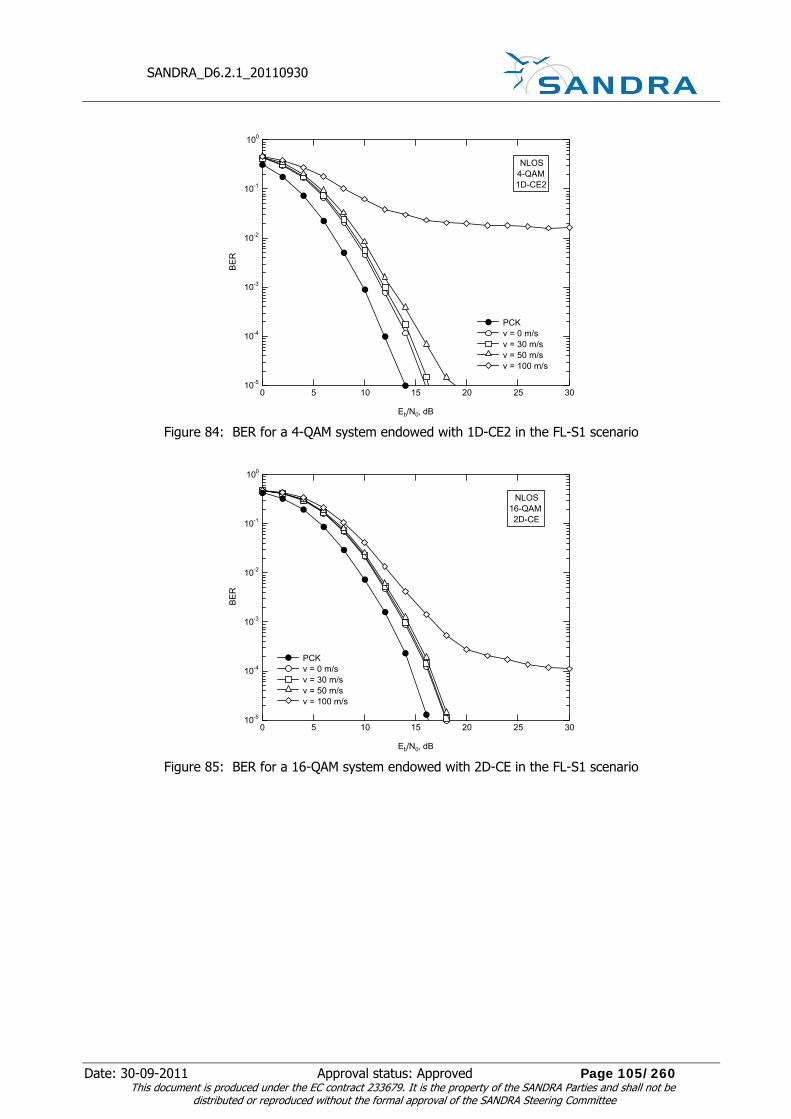
SANDRA_D6.2.1_20110930
Date: 30-09-2011 Approval status: Approved Page 105/260 This document is produced under the EC contract 233679. It is the property of the SANDRA Parties and shall not be
distributed or reproduced without the formal approval of the SANDRA Steering Committee
10-5
10-4
10-3
10-2
10-1
100
BER
302520151050
Eb/N0, dB
PCK v = 0 m/s v = 30 m/s v = 50 m/s v = 100 m/s
NLOS4-QAM1D-CE2
Figure 84: BER for a 4-QAM system endowed with 1D-CE2 in the FL-S1 scenario
10-5
10-4
10-3
10-2
10-1
100
BER
302520151050
Eb/N0, dB
PCK v = 0 m/s v = 30 m/s v = 50 m/s v = 100 m/s
NLOS16-QAM2D-CE
Figure 85: BER for a 16-QAM system endowed with 2D-CE in the FL-S1 scenario

SANDRA_D6.2.1_20110930
Date: 30-09-2011 Approval status: Approved Page 106/260 This document is produced under the EC contract 233679. It is the property of the SANDRA Parties and shall not be
distributed or reproduced without the formal approval of the SANDRA Steering Committee
10-5
10-4
10-3
10-2
10-1
100
BER
302520151050
Eb/N0, dB
PCK v = 0 m/s v = 30 m/s v = 50 m/s v = 100 m/s
NLOS16-QAM1D-CE1
Figure 86: BER for a 16-QAM system endowed with 1D-CE1 in the FL-S1 scenario
10-5
10-4
10-3
10-2
10-1
100
BER
302520151050
Eb/N0, dB
PCK v = 0 m/s v = 30 m/s v = 50 m/s v = 100 m/s
NLOS16-QAM1D-CE2
Figure 87: BER for a 16-QAM system endowed with 1D-CE2 in the FL-S1 scenario
The performance of 2D-CE in the S2 scenario is shown in Figure 88 and Figure 89 for 4-QAM and 16-QAM systems, respectively. The main difference between these results and those illustrated in Figure 82 and Figure 85 pertaining to the S1 scenario is that the slope of the BER curves is now significantly reduced, which can be explained by observing that in the S2 case the system cannot exploit all the frequency diversity offered by the propagation channel. It is also worth noting that the BER curves in Figure 89 are plagued by an irreducible error floor even when the channel is static. In such a case, the floor cannot be ascribed to channel variations but it is rather a consequence of the assumption that the channel response varies linearly in the frequency direction. Since such an assumption is also employed in the S1 scenario, we expect that an error floor occurs even in the S1 case and it is not visible in the previous figures just because it appears at very low BER values. Figure 90 and Figure 91 illustrate the sensitivity of a 4-QAM system to CFO and timing errors, respectively, in the S1 scenario. We consider several values of Eb / N0 , with the mobile speed being fixed to 30 m/s. Similar results are reported in Figure 92 and Figure 93 for a 16-QAM constellation. The CFO is normalized to the subcarrier spacing, while a timing error equal to zero in Figure 91 and Figure 93 indicates that the DFT window at the receiver side starts just at the beginning of the CP. As it is seen, the BER achieves a

SANDRA_D6.2.1_20110930
Date: 30-09-2011 Approval status: Approved Page 107/260 This document is produced under the EC contract 233679. It is the property of the SANDRA Parties and shall not be
distributed or reproduced without the formal approval of the SANDRA Steering Committee
global minimum when the timing error is 128 (equal to the CP length). In such a case, the DFT window is perfectly aligned with the useful part of the OFDM symbol.
10-5
10-4
10-3
10-2
10-1
100
BE
R
302520151050
Eb/N0, dB
PCK v = 0 m/s v = 30 m/s v = 50 m/s v = 100 m/s
NLOS4-QAM2D-CE
Figure 88 : BER for a 4-QAM system endowed with 2D-CE in the FL-S2 scenario
10-5
10-4
10-3
10-2
10-1
100
BE
R
302520151050
Eb/N0, dB
PCK v = 0 m/s v = 30 m/s v = 50 m/s v = 100 m/s
NLOS16-QAM2D-CE
Figure 89: BER for a 16-QAM system endowed with 2D-CE in the FL-S2 scenario

SANDRA_D6.2.1_20110930
Date: 30-09-2011 Approval status: Approved Page 108/260 This document is produced under the EC contract 233679. It is the property of the SANDRA Parties and shall not be
distributed or reproduced without the formal approval of the SANDRA Steering Committee
10-7
10-6
10-5
10-4
10-3
10-2
10-1
100
BER
-0.2 -0.1 0.0 0.1 0.2
residual CFO error
Eb/N 0=10dB Eb/N 0=12dB Eb/N 0=14dB Eb/N 0=16dB Eb/N 0=18dB
4-QAMNg=128
v = 30 m/s2D-CE
Figure 90: Sensitivity to CFO errors of a 4-QAM system for different SNR values in the FL-S1 scenario
10-7
10-6
10-5
10-4
10-3
10-2
10-1
100
BER
150100500-50
residual timing error
Eb/N 0=10dB Eb/N 0=12dB Eb/N 0=14dB Eb/N 0=16dB Eb/N 0=18dB
4-QAMNg=128
v = 30 m/s2D-CE
Figure 91: Sensitivity to timing errors of a 4-QAM system for different SNR values in the FL-S1 scenario

SANDRA_D6.2.1_20110930
Date: 30-09-2011 Approval status: Approved Page 109/260 This document is produced under the EC contract 233679. It is the property of the SANDRA Parties and shall not be
distributed or reproduced without the formal approval of the SANDRA Steering Committee
10-6
10-5
10-4
10-3
10-2
10-1
100
BER
-0.2 -0.1 0.0 0.1 0.2
residual CFO error
Eb/N 0=10dB Eb/N 0=12dB Eb/N 0=14dB Eb/N 0=16dB Eb/N 0=18dB
16-QAMNg=128
v = 30 m/s2D-CE
Figure 92: Sensitivity to CFO errors of a 16-QAM system for different SNR values in the FL-S1 scenario
10-6
10-5
10-4
10-3
10-2
10-1
100
BER
150100500-50
residual timing error
Eb/N 0=10dB Eb/N 0=12dB Eb/N 0=14dB Eb/N 0=16dB Eb/N 0=18dB
16-QAMNg=128
v = 30 m/s2D-CE
Figure 93: Sensitivity to timing errors of a 16-QAM system for different SNR values in the FL-S1 scenario
At this stage it is interesting to reconsider the timing and frequency estimators derived in Chapter 5 and compare their accuracy with the sensitivity of the AeroMACS to synchronization errors. For this purpose, in Figure 94 and Figure 95 we show the probability density function (pdf) of the CFO and timing estimates, respectively. These results are obtained at SNR = 10 dB by correlating the last part of the OFDM symbol with the corresponding CP. The correlation is then averaged over M B = 2 OFDMA symbols. The mobile
speed is 30 m/s and the CP has length Ng = 128 . Since the normalized CFO values are (with high
probability) smaller than 2 ⋅10−2 , from the results shown in Figure 90 and Figure 92 we expect that the system is quite robust against residual CFOs. A similar conclusion applies to residual timing errors, which do not exceed a few units and, accordingly, are expected to have a negligible impact on the error-rate performance.

SANDRA_D6.2.1_20110930
Date: 30-09-2011 Approval status: Approved Page 110/260 This document is produced under the EC contract 233679. It is the property of the SANDRA Parties and shall not be
distributed or reproduced without the formal approval of the SANDRA Steering Committee
0.5
0.4
0.3
0.2
0.1
0.0
pdf o
f CFO
est
imat
e
-0.2 -0.1 0.0 0.1 0.2
CFO
Ng=128SNR = 10 dBMB = 2v = 30 m/s
Figure 94 : Probability density function of the CFO estimate with SNR = 10 dB, Ng = 128 and M B = 2
0.35
0.30
0.25
0.20
0.15
0.10
0.05
0.00
pdf o
f tim
ing
estim
ate
-30 -20 -10 0 10 20 30
time index, d
Ng=128SNR = 10 dBMB = 2v = 30 m/s
Figure 95: Probability density function of the timing estimate with SNR = 10 dB, Ng = 128 and M B = 2
As mentioned in Chapter 4, it is convenient to shift the timing estimate by Ng / 2 samples starting from
the beginning of the CP in order to reduce the probability of occurrence of IBI at the output of the receiver DFT. Such a timing delay produces a linear phase shift of the channel response in the frequency domain, which translates into a sinusoidal variation of the real and imaginary parts of Hk (n) with the frequency
index n. This would compromise the basic assumption that Hk (n) is subject to linear variations over any cluster, thereby resulting into a substantial degradation of the channel estimation accuracy. To overcome this problem, the channel estimates at the pilot positions are counter-rotated in order to compensate for the phase shift produced by the superimposed timing delay, yielding
H ' = [H0 (0), H1(4)e j 4φ , H1(8)e j 8φ , H0 (12)e j12φ ]T (Eq.131)
with

SANDRA_D6.2.1_20110930
Date: 30-09-2011 Approval status: Approved Page 111/260 This document is produced under the EC contract 233679. It is the property of the SANDRA Parties and shall not be
distributed or reproduced without the formal approval of the SANDRA Steering Committee
φ =2πΔτNTc
(Eq.132)
and Δτ = (Ng / 2)Tc . Then, the channel parameters θ = [a,b,c]T are estimated as
θ = (AT A)−1AT H ' (Eq.133)
and the channel response over the cluster is eventually obtained in the form
Hk (n) = ak + bn + c( )e− jnφ . (Eq.134)
6.2 RL Channel Estimation
In this section we address the channel estimation task in the RL, i.e., from the users’ terminals to the BS. After illustrating the pilot arrangement employed in the AeroMACS uplink subframe, the 2D-CE scheme will be adapted to the time-frequency pilot grid employed in the RL. 6.2.1 AeroMACS Tile Structure In the RL PUSC, three consecutive OFDMA symbols form a slot, while a tile is defined as a set of four adjacent subcarriers belonging to the same slot. As shown in Figure 96, each tile has four pilots at its corners, while the remaining 8 subcarriers are used for data transmission. The pilots are taken from a BPSK constellation and are generated in a pseudo-random fashion. All the active subcarriers in the signal bandwidth are divided into six groups, each containing the same number of tiles. A tile is chosen from each group according to a pseudo-random permutation rule, and the selected tiles are joined together to construct a subchannel, which represents the minimum frequency-time resource unit allocated to an uplink user. A subchannel is thus composed of six disjoint tiles in the frequency direction, which are transmitted during the same time slot. In order to increase the time diversity offered by the wireless channel, the tiles of a specified subchannel are permuted after three symbol periods. This way, a deep long-term channel fade can extend its effect only to a relatively short time period.
time
pilot data
frequency
k=2
k=1
k=0
n=2 n=3n=1n=0
Figure 96: AeroMACS tile structure in the RL-PUSC
A disadvantage of the illustrated allocation scheme is that it greatly complicates the channel estimation task. Since the tiles of a given subchannel may be located far away in the frequency domain, channel knowledge on a given tile does not provide any useful information about the channel realization over the other tiles, similarly to what was observed in the FL. However, while in the FL it is possible to exploit the channel correlation in the time direction (if necessary), this is not feasible in the RL because the physical locations of the tiles change every time slot, thereby making very difficult to track the channel variations. In other words, while in the FL the channel estimates obtained over clusters located on the same frequency band and belonging to successive time slots can be interpolated to improve the estimation accuracy, in the

SANDRA_D6.2.1_20110930
Date: 30-09-2011 Approval status: Approved Page 112/260 This document is produced under the EC contract 233679. It is the property of the SANDRA Parties and shall not be
distributed or reproduced without the formal approval of the SANDRA Steering Committee
RL this is not feasible as these tiles are generally assigned to different uplink users. For all these reasons, channel estimation in the RL must necessarily be accomplished on a tile-by-tile basis.
6.2.2 Joint FL timing and Channel Estimation Through 2D Linear Interpolation
Timing synchronization in the RL is achieved by means of a contention-based initial ranging by which a user that intends to establish a communication link with the BS transmits a BPSK pseudo-random code over a set of 144 specific subcarriers (ranging channel). If multiple users transmit their ranging signal simultaneously, they are allowed to collide on the same ranging channel. In such a situation the accuracy of the timing estimates may be poor as a consequence of the multiuser interference. For this reason, in the RL it might be convenient for the BS to compute a refined timing estimate while performing the channel estimation task. To see how this comes about, we consider a situation where the user is assigned M tiles enumerated by an index m = 0,1,K, M −1 . Without loss of generality, we concentrate on the m-th tile with subcarrier indices n = 0,1,2, 3 and time indices k = 0,1,2 . Assuming ideal frequency synchronization, the DFT output over the tile is given by , , , ,( ) ( ) ( ) ( ) 0,1,2,3 ; 0,1, 2k m k m k m k mX n c n H n w n n k= + = = (Eq.135)
where Hk ,m(n) still denotes the channel frequency response over the n-th subcarrier of the k-th OFDMA
symbol, ck ,m(n) is the transmitted symbol (data or pilot) and wk ,m(n) is AWGN with power σw
2 . In the
RL, the pilots are taken from a BPSK constellation with unit power, i.e., ck ,m(n) ∈{±1}. The channel
response is firstly estimated at the four pilot positions as
,,
,
( )( ) {0,2} and {0,3}ˆ
( )kk m
mm
k
X nn k nH
c n= ∈ ∈ . (Eq.136)
To proceed further, we assume that the channel response over each tile varies linearly in both the time and frequency directions except for the phase shift induced by the timing error. This yields Hk ,m (n) = (amk + bmn + cm ) e jnφ (Eq.137)
where the phase φ is related to the residual timing error Δτ . We call
Hm = [H0,m (0), H2,m (0), H0,m (3), H 2,m (3)]T a vector collecting the channel estimates evaluated at the
pilot positions for the m-th cluster. Then, letting θm = [am ,bm ,cm ]T , from (Eq.136) we have
Hm = Ω(φ)Dθm + wm m = 0,1,K, M −1 (Eq.138)
where wm accounts for the noise contribution, while Ω(φ) = diag{1,1,e j 3φ ,e j 3φ} and
D =
0 0 12 0 10 3 12 3 1
⎡
⎣
⎢⎢⎢⎢
⎤
⎦
⎥⎥⎥⎥
. (Eq.139)
The LS method for the joint estimation of (φ,θ) with θ = [θ0T θ1
T L θM −1T ]T leads to the minimization of
the objective function
Λ( %φ, %θ) = Hm − Ω( %φ)D%θm
2
m=0
M −1
∑ (Eq.140)
with respect to (%φ, %θ) . Minimizing with respect to %θm yields

SANDRA_D6.2.1_20110930
Date: 30-09-2011 Approval status: Approved Page 113/260 This document is produced under the EC contract 233679. It is the property of the SANDRA Parties and shall not be
distributed or reproduced without the formal approval of the SANDRA Steering Committee
θm ( %φ) = (DH D)−1DHΩH ( %φ)Hm m = 0,1,K, M −1 (Eq.141)
which is then substituted back into (Eq.140). This produces
Ψ( %φ) = − Hm
HΩ( %φ)EΩH ( %φ)Hmm=0
M −1
∑ (Eq.142)
where we have defined
E = D(DH D)−1DH . (Eq.143)
After straightforward computations, we can rewrite Ψ( %φ) as
Ψ( %φ) = −
14
R(0) −12ℜe R(1)e− j 3 %φ + R(2){ } (Eq.144)
with
R(0) = 3 H0,m (0)2+ H1,m (4)
2+ H1,m (8)
2+ H 0,m (12)
2⎡⎣⎢
⎤⎦⎥m=0
M −1
∑
R(1) = H2,m (3) − H0,m (3)⎡⎣ ⎤⎦m=0
M −1
∑ H 2,m∗ (0) − H0,m
∗ (0)⎡⎣ ⎤⎦
R(2) = H 2,m (0)H0,m∗ (0) + H 2,m (3)H0,m
∗ (3)⎡⎣ ⎤⎦m=0
M −1
∑ .
(Eq.145)
The timing estimate is thus given by
φ =13
arg{R(1)} (Eq.146)
while the channel parameters are estimated as
θm = (DH D)−1DHΩH (φ)Hm m = 0,1,K, M −1 (Eq.147)
or, equivalently,
am =14
−H 0,m (0) + H2,m (0) − H 0,m (3)e− j 3φ + H 2,m (3)e− j 3φ⎡⎣ ⎤⎦
bm =16
−H 0,m (0) − H2,m (0) + H 0,m (3)e− j 3φ + H 2,m (3)e− j 3φ⎡⎣ ⎤⎦
cm =14
3H 0,m (0) + H2,m (0) + H 0,m (3)e− j 3φ − H 2,m (3)e− j 3φ⎡⎣ ⎤⎦ .
(Eq.148)
The channel response over the m-th tile is eventually obtained in the form
H k ,m (n) = (amk + bmn + cm )e jnφ (Eq.149)
with [am , bm , cm ]T as given in (Eq.148).
It is worth observing that, in the absence of thermal noise, the objective function Ψ( %φ) in (Eq.144) takes the form
Ψ( %φ) = K − 4 am
2
m=0
M −1
∑ cos[3(φ − %φ)] (Eq.150)
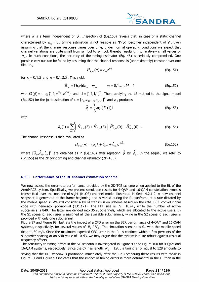
SANDRA_D6.2.1_20110930
Date: 30-09-2011 Approval status: Approved Page 114/260 This document is produced under the EC contract 233679. It is the property of the SANDRA Parties and shall not be
distributed or reproduced without the formal approval of the SANDRA Steering Committee
where K is a term independent of %φ . Inspection of (Eq.150) reveals that, in case of a static channel
characterized by am = 0 , timing estimation is not feasible as Ψ( %φ) becomes independent of %φ . Even assuming that the channel response varies over time, under normal operating conditions we expect that channel variations are quite small from symbol to symbol, thereby resulting into relatively small values of am . In such conditions, the accuracy of the timing estimator (Eq.146) is seriously compromised. One possible way out can be found by assuming that the channel response is (approximately) constant over one tile, i.e., Hk ,m (n) = cme jnφ (Eq.151)
for k = 0,1,2 and n = 0,1,2,3 . This yields
Hm = Ω(φ)dcm + wm m = 0,1,K, M −1 (Eq.152)
with Ω(φ) = diag{1,1,e j 3φ ,e j 3φ} and d = [1,1,1,1]T . Then, applying the LS method to the signal model
(Eq.152) for the joint estimation of c = [c0 ,c1,K,cM −1]T and φ , produces
φc =13
arg{Rc (1)} (Eq.153)
with
Rc (1) = H 2,m (3) + H0,m (3)⎡⎣ ⎤⎦m=0
M −1
∑ H 2,m∗ (0) + H0,m
∗ (0)⎡⎣ ⎤⎦ . (Eq.154)
The channel response is then evaluated as
H k ,m (n) = (amk + bmn + cm )e jnφc (Eq.155)
where [am , bm , cm ]T are obtained as in (Eq.148) after replacing φ by φc . In the sequel, we refer to (Eq.155) as the 2D joint timing and channel estimator (2D-TCE).
6.2.3 Performance of the RL channel estimation scheme We now assess the error-rate performance provided by the 2D-TCE scheme when applied to the RL of the AeroMACS system. Specifically, we present simulation results for 4-QAM and 16-QAM constellation symbols transmitted over the non-line-of-sight (NLOS) channel model illustrated in Sect. 4.2.1.2. A new channel snapshot is generated at the frame beginning and is varied during the RL subframe at a rate dictated by the mobile speed v. We still consider a BICM transmission scheme based on the rate 1 / 2 convolutional code with generator polynomial (131,171). The FFT size is N = 1024 , while the number of active subcarriers is 840. The latter are divided into 35 subchannels, which are allocated to the active users. In the S1 scenario, each user is assigned all the available subchannels, while in the S2 scenario each user is provided with only one subchannel. Figure 97 and Figure 98 illustrate the impact of a CFO error on the BER performance of 4-QAM and 16-QAM systems, respectively, for several values of Eb / N0 . The simulation scenario is S1 with the mobile speed fixed to 30 m/s. Since the maximum expected CFO error in the RL is confined within a few percents of the subcarrier spacing at an SNR value of 10 dB, we may argue that the system is quite robust against residual frequency offsets. The sensitivity to timing errors in the S1 scenario is investigated in Figure 99 and Figure 100 for 4-QAM and 16-QAM systems, respectively. Since the CP has length Ng = 128 , a timing error equal to 128 amounts to
saying that the DFT window is positioned immediately after the CP. Comparing these results with those in Figure 91 and Figure 93 indicates that the impact of timing errors is more detrimental in the FL than in the

SANDRA_D6.2.1_20110930
Date: 30-09-2011 Approval status: Approved Page 115/260 This document is produced under the EC contract 233679. It is the property of the SANDRA Parties and shall not be
distributed or reproduced without the formal approval of the SANDRA Steering Committee
RL since in the former case the BER curves rapidly depart from their global minimum as the timing error increases, while in the RL the BER keeps close to its minimum over a much larger interval of timing errors. This behaviour can be explained by observing that a timing offset Δτ produces a linearly increasing phase shift in the frequency domain which compromises the assumption of a linear variation of the channel frequency response over the FL cluster or RL tile. Recalling that the cluster is composed by 14 subcarriers while the tile only contains four adjacent subcarriers, it is easily understood that the impact of the aforementioned phase shift on the channel estimation accuracy is much more pronounced in the FL than in the RL. It is also worth pointing out that IBI will be present at the DFT output whenever Δτ / Tc lies
outside the interval Jd = [L −1, Ng ] , thereby leading to a performance loss that increases with the
magnitude of the timing error. This concept is validated by the results shown in Figure 99 and Figure 100, where the BER curves approach their global minimum and are nearly flat over the interval Jd . In order to reduce the probability of insurgence of IBI, timing adjustment during the ranging procedure must be made such that the receive DFT window at the BS starts (on average) in the middle point of the CP of the incoming OFDMA symbols.
10-7
10-6
10-5
10-4
10-3
10-2
10-1
100
BER
-0.2 -0.1 0.0 0.1 0.2
residual CFO error
Eb/N 0=10dB Eb/N 0=12dB Eb/N 0=14dB Eb/N 0=16dB Eb/N 0=18dB
4-QAMNg=128
v = 30 m/s
Figure 97: Sensitivity to CFO errors of a 4-QAM system for different SNR values in the RL-S1 scenario

SANDRA_D6.2.1_20110930
Date: 30-09-2011 Approval status: Approved Page 116/260 This document is produced under the EC contract 233679. It is the property of the SANDRA Parties and shall not be
distributed or reproduced without the formal approval of the SANDRA Steering Committee
10-6
10-5
10-4
10-3
10-2
10-1
100
BER
-0.2 -0.1 0.0 0.1 0.2
residual CFO error
Eb/N 0=10dB Eb/N 0=12dB Eb/N 0=14dB Eb/N 0=16dB Eb/N 0=18dB
16-QAMNg=128
v = 30 m/s
Figure 98: Sensitivity to CFO errors of a 16-QAM system for different SNR values in the RL-S1 scenario
10-7
10-6
10-5
10-4
10-3
10-2
10-1
100
BE
R
150100500-50
residual timing error
Eb/N 0=10dB Eb/N 0=12dB Eb/N 0=14dB Eb/N 0=16dB Eb/N 0=18dB
4-QAMNg=128
v = 30 m/s
Figure 99 : Sensitivity to timing errors of a 4-QAM system for different SNR values in the RL-S1 scenario

SANDRA_D6.2.1_20110930
Date: 30-09-2011 Approval status: Approved Page 117/260 This document is produced under the EC contract 233679. It is the property of the SANDRA Parties and shall not be
distributed or reproduced without the formal approval of the SANDRA Steering Committee
10-7
10-6
10-5
10-4
10-3
10-2
10-1
100
BE
R
150100500-50
residual timing error
Eb/N 0=10dB Eb/N 0=12dB Eb/N 0=14dB Eb/N 0=16dB Eb/N 0=18dB
16-QAMNg=128
v = 30 m/s
Figure 100: Sensitivity to timing errors of a 16-QAM system for different SNR values in the RL-S1 scenario
Figure 101 and Figure 102 illustrate the BER performance in the S1 scenario for 4-QAM and 16-QAM systems, respectively. These results are similar to those obtained in the FL and shown in Figure 82 and Figure 85, except that in the RL a higher floor is visible at a mobile speed of 100 m/s as compared to the FL. This can be explained by recalling that each time slot spans three consecutive OFDMA symbols in the RL and only two OFDMA symbols in the FL, thereby making channel variations much more severe over the RL tile than over the FL cluster. The error-rate obtained in the S2 scenario is reported in Figure 103 and Figure 104 for 4-QAM and 16-QAM constellations, respectively. Compared to the corresponding FL results shown in Figure 88 and Figure 89, we still observe a higher error floor at a mobile speed of 100 m/s, while improved performance is obtained at lower values of v. The reason is that in the FL only two clusters are joined together to form a subchannel, while any subchannel in the RL is decomposed into six tiles that are pseudo-randomly positioned across the signal spectrum. Since the channel gains can be considered as statistically independent over different tiles or clusters, the increased fragmentation of the RL subchannel gives the opportunity for the system to better exploit the frequency diversity offered by the propagation channel.
10-5
10-4
10-3
10-2
10-1
100
BE
R
302520151050
Eb/N0, dB
PCK v = 0 m/s v = 30 m/s v = 50 m/s v = 100 m/s
NLOS4-QAM2D-CE
Figure 101: BER for a 4-QAM system endowed with 2D-TCE in the RL-S1 scenario

SANDRA_D6.2.1_20110930
Date: 30-09-2011 Approval status: Approved Page 118/260 This document is produced under the EC contract 233679. It is the property of the SANDRA Parties and shall not be
distributed or reproduced without the formal approval of the SANDRA Steering Committee
10-5
10-4
10-3
10-2
10-1
100
BER
302520151050
Eb/N0, dB
PCK v = 0 m/s v = 30 m/s v = 50 m/s v = 100 m/s
NLOS16-QAM2D-CE
Figure 102: BER for a 16-QAM system endowed with 2D-TCE in the RL-S1 scenario
10-5
10-4
10-3
10-2
10-1
100
BER
302520151050
Eb/N0, dB
PCK v = 0 m/s v = 30 m/s v = 50 m/s v = 100 m/s
NLOS4-QAM2D-CE
Figure 103: BER for a 4-QAM system endowed with 2D-TCE in the RL-S2 scenario
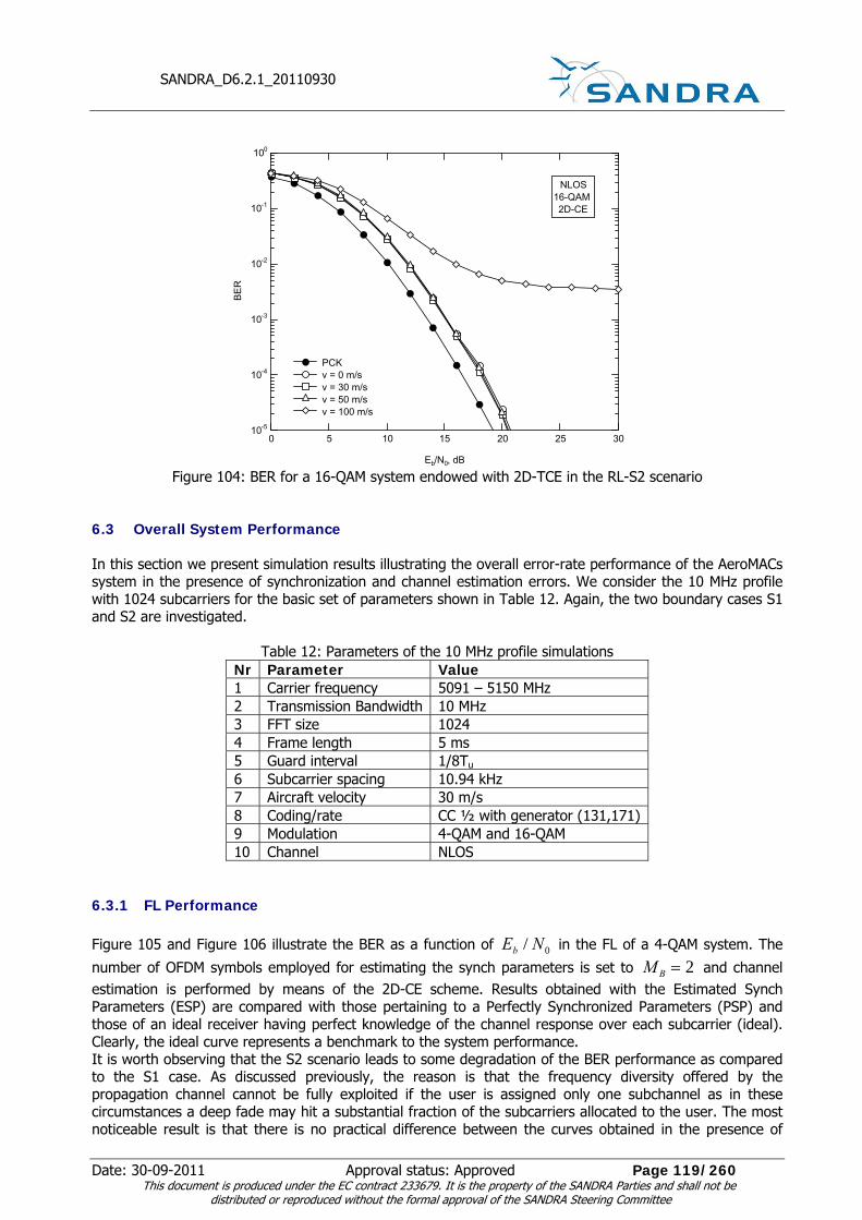
SANDRA_D6.2.1_20110930
Date: 30-09-2011 Approval status: Approved Page 119/260 This document is produced under the EC contract 233679. It is the property of the SANDRA Parties and shall not be
distributed or reproduced without the formal approval of the SANDRA Steering Committee
10-5
10-4
10-3
10-2
10-1
100
BE
R
302520151050
Eb/N0, dB
PCK v = 0 m/s v = 30 m/s v = 50 m/s v = 100 m/s
NLOS16-QAM2D-CE
Figure 104: BER for a 16-QAM system endowed with 2D-TCE in the RL-S2 scenario
6.3 Overall System Performance
In this section we present simulation results illustrating the overall error-rate performance of the AeroMACs system in the presence of synchronization and channel estimation errors. We consider the 10 MHz profile with 1024 subcarriers for the basic set of parameters shown in Table 12. Again, the two boundary cases S1 and S2 are investigated.
Table 12: Parameters of the 10 MHz profile simulations Nr Parameter Value 1 Carrier frequency 5091 – 5150 MHz 2 Transmission Bandwidth 10 MHz 3 FFT size 1024 4 Frame length 5 ms 5 Guard interval 1/8Tu 6 Subcarrier spacing 10.94 kHz 7 Aircraft velocity 30 m/s 8 Coding/rate CC ½ with generator (131,171) 9 Modulation 4-QAM and 16-QAM 10 Channel NLOS
6.3.1 FL Performance Figure 105 and Figure 106 illustrate the BER as a function of Eb / N0 in the FL of a 4-QAM system. The
number of OFDM symbols employed for estimating the synch parameters is set to M B = 2 and channel estimation is performed by means of the 2D-CE scheme. Results obtained with the Estimated Synch Parameters (ESP) are compared with those pertaining to a Perfectly Synchronized Parameters (PSP) and those of an ideal receiver having perfect knowledge of the channel response over each subcarrier (ideal). Clearly, the ideal curve represents a benchmark to the system performance. It is worth observing that the S2 scenario leads to some degradation of the BER performance as compared to the S1 case. As discussed previously, the reason is that the frequency diversity offered by the propagation channel cannot be fully exploited if the user is assigned only one subchannel as in these circumstances a deep fade may hit a substantial fraction of the subcarriers allocated to the user. The most noticeable result is that there is no practical difference between the curves obtained in the presence of

SANDRA_D6.2.1_20110930
Date: 30-09-2011 Approval status: Approved Page 120/260 This document is produced under the EC contract 233679. It is the property of the SANDRA Parties and shall not be
distributed or reproduced without the formal approval of the SANDRA Steering Committee
synchronization errors and those pertaining to the perfectly synchronized system. This means that the designed synchronization algorithms entail a negligible loss in the error-rate performance of the AeroMACS system. A similar conclusion applies to a 16-QAM system, as it can be inferred from the results shown in Figure 107 and Figure 108.
10-5
10-4
10-3
10-2
10-1
100
BE
R
302520151050
Eb/N0
Ideal PSP ESP
S1 scenario4-QAMNg=128MB = 2
v = 30 m/s2D-CE
Figure 105: BER of a 4-QAM system in the S1 scenario
10-5
10-4
10-3
10-2
10-1
100
BE
R
302520151050
Eb/N0
Ideal PSP ESP
S2 scenario4-QAMNg=128MB = 2
v = 30 m/s2D-CE
Figure 106: BER of a 4-QAM system in the S2 scenario

SANDRA_D6.2.1_20110930
Date: 30-09-2011 Approval status: Approved Page 121/260 This document is produced under the EC contract 233679. It is the property of the SANDRA Parties and shall not be
distributed or reproduced without the formal approval of the SANDRA Steering Committee
10-5
10-4
10-3
10-2
10-1
100
BE
R
302520151050
Eb/N0
Ideal PSP ESP
S1 scenario16-QAMNg=128MB = 2
v = 30 m/s2D-CE
Figure 107: BER of a 16-QAM system in the S1 scenario
10-5
10-4
10-3
10-2
10-1
100
BE
R
302520151050
Eb/N0
Ideal PSP ESP
S2 scenario16-QAMNg=128MB = 2
v = 30 m/s2D-CE
Figure 108: BER of a 16-QAM system in the S2 scenario
6.3.2 RL Performance
We now assess the overall performance of the RL AeroMACS system. Frequency recovery is not accomplished in the RL as the CFO estimates computed by the user terminal during the downlink phase are accurate enough and can be used in the subsequent uplink phase. In contrast, timing estimation and compensation is achieved by means of the IR procedure under the assumption that U codes are simultaneously active in the ranging channel. In our simulations we set U = 1, 4, or 8 , while channel estimation is performed by means of the 2D-TCE scheme. Similarly to what we made for the FL, results obtained with the estimated parameters (ESP) are compared with those pertaining to a perfectly synchronized system (PSP) and those provided by an ideal receiver having perfect knowledge of the channel response over each subcarrier. Figure 109 and Figure 110 illustrate the BER as a function of Eb / N0 in the RL of a 4-QAM system under the S1 and S2 scenarios, respectively. Although some performance degradation is observed in passing from the S1 to the S2 case, such degradation is not as evident as in the FL. The reason is that in the RL there is

SANDRA_D6.2.1_20110930
Date: 30-09-2011 Approval status: Approved Page 122/260 This document is produced under the EC contract 233679. It is the property of the SANDRA Parties and shall not be
distributed or reproduced without the formal approval of the SANDRA Steering Committee
a greater fragmentation of the subchannels, which allows the system to better exploit the channel frequency diversity. It is worth pointing out that no practical difference is visible between the curves obtained in the presence of synchronization errors and those pertaining to the perfectly synchronized system. This means that the IR synchronization algorithms entail a negligible loss in the error-rate performance of the AeroMACS system. The BER for a 16-QAM system is shown in Figure 111 and Figure 112. The results are similar to those in Figure 109 and Figure 110 except for the ESP curve with U = 8 . In the latter case, we observe a remarkable performance loss between the PSP and ESP curves in both the S1 and S2 scenarios. However, it is worth noting that letting U = 8 amounts to saying that 8 users are simultaneously trying to perform network entry by choosing the same IR subchannel, a situation which is expected to occur with low probability in the AeroMACS system.
10-5
10-4
10-3
10-2
10-1
100
BE
R
302520151050
Eb/N0
Ideal PSP ESP (U=1) ESP (U=4) ESP (U=8)
S1 scenario4-QAMNg=128
v = 30 m/s2D-TCE
Figure 109: BER of a 4-QAM system in the S1 scenario
10-5
10-4
10-3
10-2
10-1
100
BE
R
302520151050
Eb/N0
Ideal PSP ESP (U=1) ESP (U=4) ESP (U=8)
S2 scenario4-QAMNg=128
v = 30 m/s2D-TCE
Figure 110: BER of a 4-QAM system in the S2 scenario

SANDRA_D6.2.1_20110930
Date: 30-09-2011 Approval status: Approved Page 123/260 This document is produced under the EC contract 233679. It is the property of the SANDRA Parties and shall not be
distributed or reproduced without the formal approval of the SANDRA Steering Committee
10-5
10-4
10-3
10-2
10-1
100
BE
R
302520151050
Eb/N0
Ideal PSP ESP (U=1) ESP (U=4) ESP (U=8)
S1 scenario16-QAMNg=128
v = 30 m/s2D-TCE
Figure 111: BER of a 16-QAM system in the S1 scenario
10-5
10-4
10-3
10-2
10-1
100
BE
R
302520151050
Eb/N0
Ideal PSP ESP, 1_1, time_fine ESP, 4_1, time_fine ESP, 8_1, time_fine
S2 scenario16-QAMNg=128
v = 30 m/s2D-TCE
Figure 112: BER of a 16-QAM system in the S2 scenario
6.4 Conclusions
This chapter deals with the channel estimation problem in the AeroMACS system. Although many channel estimation techniques are available in the literature, we focused on deriving an estimation technique that is specifically tailored for the pilot arrangement employed in the AeroMACS system and involving low computational and hardware complexity. In Sect. 2 we present three channel estimation schemes for the FL transmission, namely, 2D-CE, 1D-CE1 and 1D-CE2, all based on the least-squares (LS) principle. In particular, the 2D-CE assumes that the channel response over the cluster varies linearly in both the time and frequency directions; 1D-CE1 assumes that the channel response keeps approximately constant over two consecutive OFDMA symbols and varies linearly in the frequency direction; 1D-CE2 assumes that the channel response keeps approximately constant over two consecutive OFDMA symbols and varies in a parabolic manner in the frequency direction. The accuracy of the aforementioned estimation methods has been assessed by means of computer simulations under the assumption of ideal timing and frequency

SANDRA_D6.2.1_20110930
Date: 30-09-2011 Approval status: Approved Page 124/260 This document is produced under the EC contract 233679. It is the property of the SANDRA Parties and shall not be
distributed or reproduced without the formal approval of the SANDRA Steering Committee
synchronization. We found that, compared to an ideal receiver having perfect knowledge of the channel response, all the considered schemes entail a loss of approximately 2 dB when the channel is static. Furthermore, we see that 2D-CE, differently from the 1D-CE schemes, exhibits a remarkable resilience against channel variations induced by the mobile speed. In Sect. 3 we address the channel estimation task in the reverse link (RL). Since 2D-CE provides much better results than the alternative 1D scheme, we considered only 2D-CE for channel estimation. Actually, since in the reverse link the accuracy of the timing estimates may be poor as a consequence of the multiuser interference, we derived a joint timing and channel estimation (2D-TCE) scheme in order to refine the timing estimate. Eventually, in Sect. 4 we assess the overall error-rate performance of the AeroMACS system in the presence of residual timing and frequency synchronization errors in both the forward and reverse links. Results obtained with the estimated synch parameters (ESP) are compared with those pertaining to a perfectly synchronized system (PSS). The most noticeable result is that there is no practical difference between the curves obtained in the presence of synchronization errors and those pertaining to the ideal system. This means that the designed synchronization algorithms entail a negligible loss in the error-rate performance of the AeroMACS system.
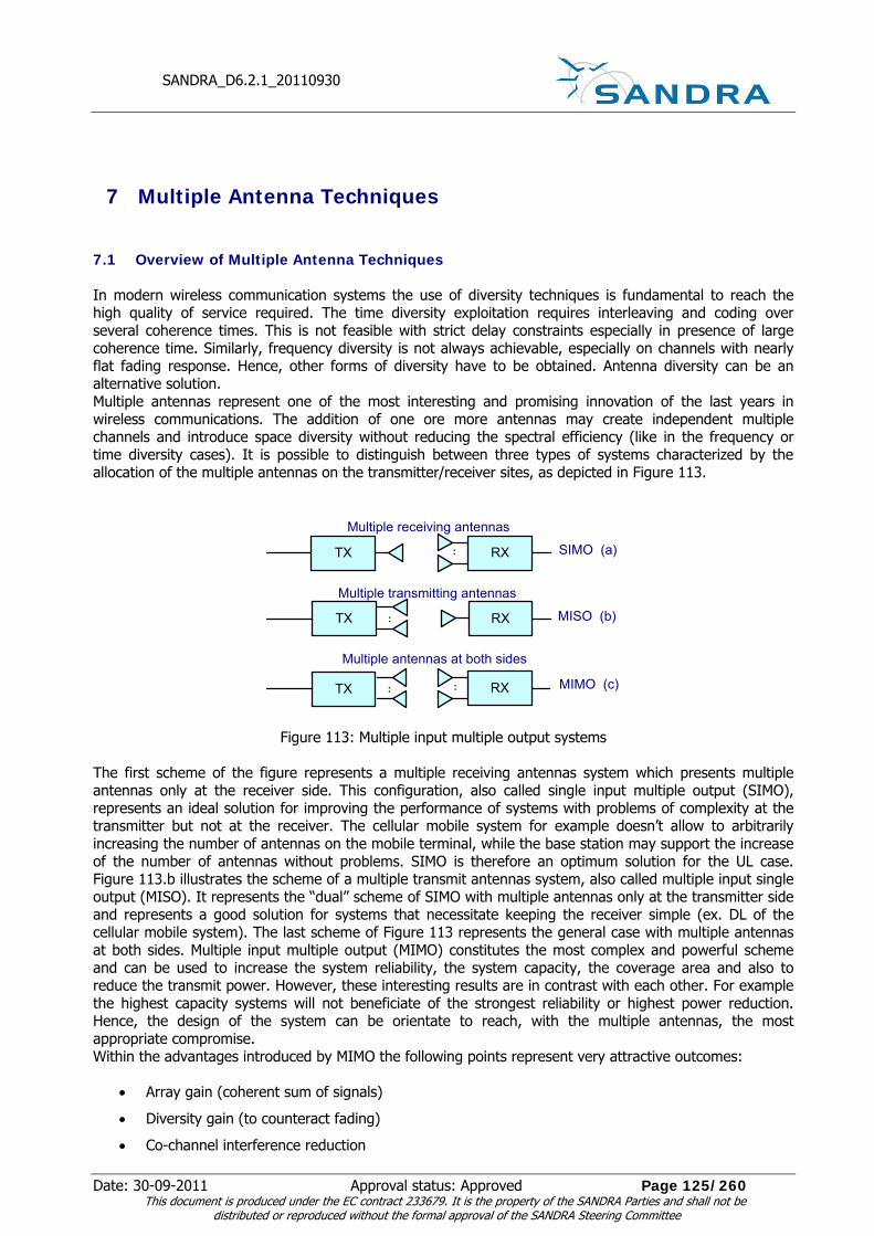
SANDRA_D6.2.1_20110930
Date: 30-09-2011 Approval status: Approved Page 125/260 This document is produced under the EC contract 233679. It is the property of the SANDRA Parties and shall not be
distributed or reproduced without the formal approval of the SANDRA Steering Committee
7 Multiple Antenna Techniques
7.1 Overview of Multiple Antenna Techniques
In modern wireless communication systems the use of diversity techniques is fundamental to reach the high quality of service required. The time diversity exploitation requires interleaving and coding over several coherence times. This is not feasible with strict delay constraints especially in presence of large coherence time. Similarly, frequency diversity is not always achievable, especially on channels with nearly flat fading response. Hence, other forms of diversity have to be obtained. Antenna diversity can be an alternative solution. Multiple antennas represent one of the most interesting and promising innovation of the last years in wireless communications. The addition of one ore more antennas may create independent multiple channels and introduce space diversity without reducing the spectral efficiency (like in the frequency or time diversity cases). It is possible to distinguish between three types of systems characterized by the allocation of the multiple antennas on the transmitter/receiver sites, as depicted in Figure 113.
TX RX..
Multiple receiving antennas
TX RX.. MISO (b)
TX .. RX.. MIMO (c)
SIMO (a)
Multiple transmitting antennas
Multiple antennas at both sides
Figure 113: Multiple input multiple output systems The first scheme of the figure represents a multiple receiving antennas system which presents multiple antennas only at the receiver side. This configuration, also called single input multiple output (SIMO), represents an ideal solution for improving the performance of systems with problems of complexity at the transmitter but not at the receiver. The cellular mobile system for example doesn’t allow to arbitrarily increasing the number of antennas on the mobile terminal, while the base station may support the increase of the number of antennas without problems. SIMO is therefore an optimum solution for the UL case. Figure 113.b illustrates the scheme of a multiple transmit antennas system, also called multiple input single output (MISO). It represents the “dual” scheme of SIMO with multiple antennas only at the transmitter side and represents a good solution for systems that necessitate keeping the receiver simple (ex. DL of the cellular mobile system). The last scheme of Figure 113 represents the general case with multiple antennas at both sides. Multiple input multiple output (MIMO) constitutes the most complex and powerful scheme and can be used to increase the system reliability, the system capacity, the coverage area and also to reduce the transmit power. However, these interesting results are in contrast with each other. For example the highest capacity systems will not beneficiate of the strongest reliability or highest power reduction. Hence, the design of the system can be orientate to reach, with the multiple antennas, the most appropriate compromise. Within the advantages introduced by MIMO the following points represent very attractive outcomes:
• Array gain (coherent sum of signals)
• Diversity gain (to counteract fading)
• Co-channel interference reduction

SANDRA_D6.2.1_20110930
Date: 30-09-2011 Approval status: Approved Page 126/260 This document is produced under the EC contract 233679. It is the property of the SANDRA Parties and shall not be
distributed or reproduced without the formal approval of the SANDRA Steering Committee
• Spatial multiplexing (to achieve high spectral efficiency).
The array gain is one of the easiest forms of gain achievable by the MIMO systems. It is typical of systems with multiple receiving antennas since it comes from the coherent sum of received signals. The array gain GA is linearly proportional to the number of antennas (GA [dB] = 10*log10NR) and can be obtained also in case of statistically correlated channels. Diversity gain results from the multiple independent channels between the transmitter and the receiver. By averaging over different independent signal paths, the probability that the overall gain is small decreases. Being a result of the statistical richness of those channels, the diversity gain disappears if the channels are correlated. Moreover, it may be obtained by all the types of configuration: SIMO, MISO and MIMO. Differently form the array gain, the diversity gain saturates with the increasing number of antennas [TSE_05]. Several systems operating in congested bands (for example the VHF) suffer from co-channel interference. Multiple antennas in these cases can be used for reducing the interferences of undesired signals over the same bandwidth [WIN_84], [CHI_08], [CHI_03nov], [Errore. L'origine riferimento non è stata trovata.]. Last, but very important, MIMO may be used for achieving a high spectral efficiency system. The different “sub-channels” created by the multiple antennas may be used for transmitting different data streams in parallel and creating a spatial multiplexing. Spatial multiplexing exploits the multipath richness of the environment and increases the capacity of the system. Differently from the previous benefit introduced by multiple antennas, spatial multiplexing can be only done with true MIMO systems (i.e. with multiple antennas at both sides). The wireless channels commonly present a slow and a fast fading component. The fast fading caused by the scattered environment negatively affects the performance of a single input single output (SISO) system, but can be exploited by MIMO for achieving diversity and hence, increasing the reliability or the capacity. In a scattered environment, in fact, it is possible to obtain independently faded replicas of the signal by different means. The physical separation of the antennas (spatial separation) is the simplest way. The required distance between antennas depends on the local scattering and on the carrier frequency. For a mobile on the ground with many scatterers, a distance S between one wave length and a quarter of it may be sufficient (S>λ/4). For high towers the required distance is much bigger, up to several wavelengths. Other efficient ways of obtaining independent replicas of the signals are polarization and angle direction. These techniques produce different types of diversity and provide respectively polarization and direction (or angle) diversity. In the following sections the main characteristics of the MIMO systems will be described, focusing on the simpler cases of transmit diversity and receive diversity. Detailed descriptions of the 1x2 SIMO and 2x1 MISO systems will be also provided. For completeness an overview to the spatial multiplexing and V-BLAST concepts will be also included at the end of the chapter. Co-channel interference cancellation techniques will not be analyzed in this document; a detailed description may be found in [WIN_84], [CHI_08], [CHI_03nov].
7.1.1 Receive Diversity – SIMO
One of the simplest ways to obtain antenna diversity is the addition of one or more antennas only at the receiver side of the system. This SIMO scheme permits to increase the SNR of the system combining the received versions of the signal. The simplest receive diversity case 1x2 SIMO, with 1 antenna at the transmitter side and 2 at the receiver side, is represented in Figure 114. It is possible to characterize the system using a vector form summarizing the two received signals y1 = x h1 + n1 and y2 = x h2 + n2 with a unique vector y = x h + n, where the vectors h and n represent respectively the channel gains and the noise contributions.

SANDRA_D6.2.1_20110930
Date: 30-09-2011 Approval status: Approved Page 127/260 This document is produced under the EC contract 233679. It is the property of the SANDRA Parties and shall not be
distributed or reproduced without the formal approval of the SANDRA Steering Committee
Figure 114: 1x2 SIMO scheme As previously mentioned, in the multiple receiving antenna case, beside the diversity gain, there is an array (or power) gain. Being not related to the statistical properties of the channels, it increases the system’s SNR also in case of correlated channels as in LOS channels. The array gain is linearly proportional to the number of antennas (SNRxNr) and doesn’t have saturation. For example in the case of two antennas it introduces a 3-dB gain and for every doubling of antennas adds other 3-dB gain. The most common ways to combine the received signals are selection combining and maximal ratio combining.
7.1.1.1 Selection Combining
Selection Combining (SC) represents the simplest algorithm for exploiting the antenna diversity. It instantly analyzes the received power over all the branches corresponding to the different antennas and then selects the one with highest power. Figure 115 and Figure 116 show respectively the scheme of SC and an example of total SNR. The useful energy of the branches non-selected is lost. It is clear that the SC algorithm is not optimum, however, its simple implementation constitutes the main strength point. Figure 117 provides the average bit error probability of SC over Rayleigh fading channel.
Figure 115: Selection combining scheme
Figure 116: Resulting SNR with selection combining

SANDRA_D6.2.1_20110930
Date: 30-09-2011 Approval status: Approved Page 128/260 This document is produced under the EC contract 233679. It is the property of the SANDRA Parties and shall not be
distributed or reproduced without the formal approval of the SANDRA Steering Committee
Figure 117: SC Performance over Rayleigh fading (figure taken from [AND_07])
7.1.1.2 Weight and Combine and Maximum Ratio Combining
Weight and combine algorithms exploit better the overall received energy with respect to SC, by weighting and then adding all the signals corresponding to all the branches of the system receiver
*1
Nry y wi ii= ×∑
=. (Eq.156)
Maximum Ratio Combining (MRC) is a weight and combine algorithm with the weights chosen proportional to the channel (wi = hi). A generic 1x2 SIMO system receiver with MRC is represented in Figure 118. The received signals y1 and y2 are multiplied by the conjugate values of the corresponding channel coefficients. It is therefore necessary to have at the receiver full channel information (amplitude and phase). The multiplication of the signal by h1/2
* means that the phase delay introduced by the channel is fully compensated and that the signals are coherently added.
Figure 118: 1x2 SIMO with MRC receiver scheme
The SNR of the system can be obtained considering the two SNRs corresponding to the two branches (SNR1 and SNR2).
2*21 1 1
1 2 2
( )( )E x h x h hSNR E x
σ σ
⎡ ⎤× ×⎣ ⎦ ⎡ ⎤= = ×⎣ ⎦
(Eq.157)

SANDRA_D6.2.1_20110930
Date: 30-09-2011 Approval status: Approved Page 129/260 This document is produced under the EC contract 233679. It is the property of the SANDRA Parties and shall not be
distributed or reproduced without the formal approval of the SANDRA Steering Committee
22 2
2 2
hSNR E x
σ⎡ ⎤= ×⎣ ⎦
. (Eq.158)
The transmitted signal can be obtained by the ML approach,
2ˆ ˆarg max ( | , ) arg min -x
x p y x h Þ x xh y= = . (Eq.157)
Applying 2 2
1 1 2 2( - ) ( - )0
x h y x h yx
⎡ ⎤∂ × + ×⎣ ⎦ =∂
we obtain
1 1 2 222 2
1 2
ˆTy h y h h yx
h h h× + ×
= =+
, (Eq.158)
while in the complex case the value of x is given by 2ˆHh yxh
= . (Eq.159)
The received signal is the sum of the transmitted signal and a variable part following a Gaussian process with zero mean, i.e.
22
1 1
1ˆ / ( ( ) )Nr Nr
H Hi i i i i i
i i
x y h h h x n hh= =
⎛ ⎞= × = + ×⎜ ⎟⎝ ⎠∑ ∑ and
2
2~ 0,n Nhσ⎛ ⎞
⎜ ⎟⎜ ⎟⎝ ⎠
. (Eq.160)
Therefore we can obtain with the previous equations the total SNR of the system,
2 22
2 22
ˆ ˆ
/out
E x E xSNR h
h σσ
⎡ ⎤ ⎡ ⎤⎣ ⎦ ⎣ ⎦= = (Eq.161)
Explicitly for two branches, the total SNR is the sum of the two SNRs corresponding to the single ways,
2 21 2 1 22 2
t tout
P PSNR h h SNR SNRσ σ
= × + × = + , (Eq.162)
with 2
tP E x⎡ ⎤= ⎣ ⎦ .
MRC provides both array and diversity gain. In presence of correlated channel (i.e. in LOS cases) there is only the array gain that in this example amounts to 3 dB. It is possible to show that the total SNR is the maximum possible SNR; therefore this algorithm is called maximal ratio combiner. Though, it should be noted that MRC may not be optimal in some cases, since it completely ignores the interference powers. In these cases other receivers may perform better, as illustrated in the next section. Figure 119 provides the performance of MRC over Rayleigh fading for a BPSK system with respectively 1, 2, and 4 branches (starting from the right). The figure representing the average bit error probability (BEP) versus the average SNR shows the large improvement introduced in all the cases by MRC. The slope of the charts is doubled for every multiplication of the number of antennas. For a cellular system with interference limits, like WiMAX or AeroMACS, MRC might be strongly preferred to SC, despite its bigger complexity. Although MRC and SC present similar results (Figure 119 and Figure 118), (they have in fact the same diversity order); MRC introduces an array gain which can be very useful in some power limitation situations or LOS cases. Moreover, in frequency-selective fading channels, MRC can exploit all the frequency diversity, while a selection algorithm would simply select the best average received signal keeping potentially deep fades at certain frequencies.

SANDRA_D6.2.1_20110930
Date: 30-09-2011 Approval status: Approved Page 130/260 This document is produced under the EC contract 233679. It is the property of the SANDRA Parties and shall not be
distributed or reproduced without the formal approval of the SANDRA Steering Committee
Figure 119: MRC performance with Rayleigh fading (figure taken [AND_07])
7.1.1.3 SIMO with Interference
In the previous cases SIMO has been analyzed in condition of no interference. In this case a more realistic situation is considered and an interference signal xI is added to the SIMO system as represented in Figure 120. Assuming the interfering signal xI a random variable with zero mean, the received signal y is given by
I Iy hx h x n hx n= + + = + % . (Eq.163)
The overall noise I In h x n= +% is not “white” as in the previous case and has an auto-covariance matrix equal to
2 2( )HI I IR E x h h Iσ⎡ ⎤= +⎣ ⎦ . (Eq.164)
In order to maximize the Signal to Interference Noise Ratio (SINR) the received signal is multiplied by
-1/2R , and then the MRC principle is applied. The resulting scheme is equivalent to the Minimum Mean Square Error (MMSE) receiver and is called Optimum Combining (OC) receiver.
Figure 120: SIMO with interference scheme

SANDRA_D6.2.1_20110930
Date: 30-09-2011 Approval status: Approved Page 131/260 This document is produced under the EC contract 233679. It is the property of the SANDRA Parties and shall not be
distributed or reproduced without the formal approval of the SANDRA Steering Committee
7.1.2 Transmit Diversity – MISO
The multiple transmit antennas system presents multiple antennas only at the transmitter side. The MISO configuration can be particularly useful in the DL of system where the addition of antennas is feasible only on the base station. Transmit diversity schemes offer two ways of realization respectively based on open loop and close loop scheme. Close and open loop indicate the presence of a return link with Channel State Information (CSI) or not. The close loop scheme offers the advantage of the coherent sum of the different signals and hence an array gain, though the CSI at the transmitter side is often difficult to obtain, especially in presence of rather fast channels. The open loop scheme applying Space Time Coding (STC) has been only lately introduced [ALA_98] and offers a good alternative for all the systems that cannot have CSI at the transmitter side.
7.1.2.1 MISO Beamforming (Close Loop)
The MISO close loop system is based on the instantaneous transmission of weighted versions of the signal. The weights are proportional to the channel and therefore channel state information is required. Figure 121 provides a simple scheme of a 2x1 MISO system.
α1
α2
xy
nh2
h1
Figure 121: 2x1 MISO beamforming scheme
Here, 1α and 2α are the weighting factors and are chosen accordingly to satisfy 2 2
1 2 1α α+ = in order to
keep an average transmitted power 2
tP E x⎡ ⎤= ⎣ ⎦ . The received signal y is given by
1 1 2 2( )y h h x nα α= + + . (Eq.165)
Taking = *1 1α kh , = *
2 2α kh , with k =1/ h we obtain
2 21 2h h
y x n h x nh+
= + = + , and 2
22
| |OUT
E xSNR h
σ
⎡ ⎤⎣ ⎦= . (Eq.166)
This is exactly the same result obtained for the SIMO 2x1 MRC case. Though, in this case the transmitter must know phase and amplitude of both the channels (CSI at TX) which are difficult to obtain.
In this case the transmitter adjusts the transmit vector toward the receiver in terms of channel propagation vectors and therefore it is called beamforming. The beamforming doesn’t refer to the direction but to the propagation vectors (including multipath).

SANDRA_D6.2.1_20110930
Date: 30-09-2011 Approval status: Approved Page 132/260 This document is produced under the EC contract 233679. It is the property of the SANDRA Parties and shall not be
distributed or reproduced without the formal approval of the SANDRA Steering Committee
7.1.2.2 Extensions Towards MIMO: MIMO Beamforming (Eigenbeamforming)
Figure 122: MIMO beamforming scheme The MISO 2x1 beamforming case can be generalized obtaining the beamforming MIMO case depicted in Figure 122. The system with Nt transmit antennas and Nr receive antennas is described by
1 1 11 12 1 1
2 2 21 22 2 2
y x h h ny x h h n
αα
⎡ ⎤ ⎡ ⎤ ⎡ ⎤ ⎡ ⎤ ⎡ ⎤= × × +⎢ ⎥ ⎢ ⎥ ⎢ ⎥ ⎢ ⎥ ⎢ ⎥
⎣ ⎦ ⎣ ⎦ ⎣ ⎦ ⎣ ⎦ ⎣ ⎦ (Eq.167)
or y x H n y x h nα= × × + = = × +% , (Eq.168)
where %h =Hα and α represents the transmit weigthing factor vector. Imposing21 tÞ E x Pα ⎡ ⎤= =⎣ ⎦ ,
indicating the receive weighting factors with ⋅ %w =k h the SNR becomes
( )2
2tPSNR hα
σ= % . (Eq.169)
The optimum α which maximizes SNR is equal to the eigenvector of HH H corresponding to the largest eigenvalue of HH H (λMAX). The resulting SNR is given by
2
2
| |OUT MAX
E xSNR λ
σ
⎡ ⎤⎣ ⎦= . (Eq.170)
Having CSI at receiver and transmitter sides, the MIMO beamforming case provides the maximum SNR.
7.1.2.3 Space-Time Coding (Open-Loop)
STC scheme introduced by Alamouti in [ALA_98] offers a solution for all the systems where it is impossible to have reliable CSI at the transmitter side. This open loop system transmits at the same time over the different antennas combinations of the signals to transmit and it provides the same diversity gain offered by the classical maximal-ratio receive combining scheme or the beamforming with an equal number of branches. The unique requirement of the system concerns the coherence time of the channel. It is necessary to have a sufficiently slow channel, in order to allow the decoding of the signal transmitted over two (or more) antennas and consecutive time instances. In the case 2x1, the two transmitting antennas at a certain symbol period t1 transmit two different signals s1 and s2, respectively. In the following symbol period t2 the first antenna transmits s2
*, while the second one −s1*, as indicated in Figure 123.

SANDRA_D6.2.1_20110930
Date: 30-09-2011 Approval status: Approved Page 133/260 This document is produced under the EC contract 233679. It is the property of the SANDRA Parties and shall not be
distributed or reproduced without the formal approval of the SANDRA Steering Committee
Figure 123: 2x1 STC Alamouti’s scheme Assuming the channel constant over the transmission of the two symbols s1 and s2 (h1 (t1) ≈ h1 (t2) = h1 and h2 (t1) ≈ h2 (t2) = h2), the received signals r1 = r (t1) and r2 = r (t2) become
1 1 1 2 2 1y x h x h n= + + (Eq.171)
* *2 2 1 1 2 2-y x h x h n= + (Eq.172)
1 1 2 1 1* * *2 2 1 2 2-
y h h x ny h h x n
⎛ ⎞ ⎛ ⎞⎛ ⎞ ⎛ ⎞= +⎜ ⎟ ⎜ ⎟⎜ ⎟ ⎜ ⎟
⎝ ⎠ ⎝ ⎠⎝ ⎠ ⎝ ⎠ or with vectors y Hx n= + .
They can be easily decomposed in order to obtain the original symbols multiplying them by HH . If H is
orthogonal then 2HH H h I= and
2HH y h x n= + , (Eq.173) * *
1 1 1 2 2ˆ -x y h y h= , (Eq.174) * *
2 1 2 2 1x y h y h= + . (Eq.175)
Focusing on the symbol s1, it is easy to demonstrate that the resulting SNR is the same as the one obtained
for MRC,
2
21 2
E xSNR h
σ
⎡ ⎤⎣ ⎦= .
The diversity gain is 2 for the detection of each symbol, as in a 1x2 SIMO system. However, in this case the total transmitted power is twice as that transmitted by the 1x2 MRC, so there is a loose of 3 dB (corresponding to the price paid for not having a coherent sum). There isn’t in fact array gain without CSI at the transmitter. Generalized to orthogonal design in [TAR_99][TAR_99mar], the Alamuti scheme is perfectly suitable for OFDM systems. In this case, besides the coding in time direction (STC), it is possible to perform a frequency direction coding called Space Frequency Coding (SFC).
7.1.2.4 Extension Toward MIMO: MIMO STC
The MIMO 2x2 case is a generalization of the 2x1 case. In this case the total number of antennas is 4: 2 transmit and 2 receive. The receiver is composed by two “STC branches” combined with MRC. The 2x2 scheme reach a diversity order 4, the double of the 2x1 STC scheme. As showed in [ALA_98] for a Rayleig fading, this scheme provides curve with a double slope with respect to the 2x1 STC case. Moreover, exploiting a coherent sum of the signals, the 2x2 scheme provides an additional array gain. The result is also similar to the ones provided by a 1x4 SIMO MRC scheme. However, the SIMO case presents a bigger array gain coming by the 4 receive antennas (2x2 has an array gain only over 2 antennas).

SANDRA_D6.2.1_20110930
Date: 30-09-2011 Approval status: Approved Page 134/260 This document is produced under the EC contract 233679. It is the property of the SANDRA Parties and shall not be
distributed or reproduced without the formal approval of the SANDRA Steering Committee
7.1.2.5 Delay and Phase Diversity
In the multiple transmit antennas case the multicarrier systems offer the possibility of using also other diversity techniques as Delay Diversity (DD), Phase Diversity (PD) and Cyclic Delay Diversity (CDD). All these techniques artificially increase the frequency and the time selectivity of the channel by introducing additional constructive delayed and phase shifted signals. DD, PD and CDD are conditionally equal as is showed in [[DAM_01] and have the considerable advantage of being implementable by existing standards.
7.1.2.5.1 Delay Diversity
The Delay diversity scheme, introduced in [SES_94] and described in [KAI_00], is based on the instantaneous transmission of delayed replicas of the OFDM signal. The multiple antennas transmit instantaneously Nt versions of the signal. Each one differing for a specific delay δn (n=1…Nt-1). In order to assure frequency selective fading the delays have to satisfy the requirement δn ≥ kn/B, with the constant factor k ≥1 and B the total bandwidth of the system. Figure 124 shows the block diagram of an OFDM system with Nt transmit antennas and DD. Before the shifting, an additional cyclic prefix as guard interval may be inserted. The UC blocks stands for up-conversion from the baseband into the RF-band and the δs represent simple time shifts. The main disadvantaged of this system consist in the increase of the total delay spread and therefore in the necessity of increasing the cyclic prefix which reduces the spectral efficiency of the system.
Figure 124: Transmitter block scheme with delay diversity
7.1.2.5.2 Phase Diversity
The phase diversity system is based on the transmission of shifted version of the signals. The signals corresponding to each antennas are shifted by Φn,u (the indexes n=1,…Nt-1 and u=0,…Nc-1 represent the antenna number and the sub-carrier specific phase offset [KAI_00]) before the OFDM transformation. A frequency selective fading channel over the system bandwidth B is assured by the fulfillment of Φn,u ≥ 2π u/Nc; while the increasing of the frequency diversity by multiple transmit antennas is assured by a phase offset satisfying Φn,u ≥ 2π k n u/Nc (with the constant K ≥1). This system overpasses the problem of the spectral efficiency reduction; though, multiplies the number of the IFFT transformation blocks by the number of antennas.
Cyclic Delay Diversity CDD represents an efficient implementation of PD which doesn’t require the addition of IFFT blocks at the transmitter side. CDD exploits the cyclic property of the Fourier transform and avoids increasing the number of IFFT operations. As showed in the Figure 125 scheme, the OFDM symbols of the CDD signal can be generated from the reference signal just by applying a cyclic time shift δcyc to the OFDM signal and by subsequent insertion of the cyclic prefix.

SANDRA_D6.2.1_20110930
Date: 30-09-2011 Approval status: Approved Page 135/260 This document is produced under the EC contract 233679. It is the property of the SANDRA Parties and shall not be
distributed or reproduced without the formal approval of the SANDRA Steering Committee
Figure 125: CDD transmitter scheme It is also possible to apply CDD to the receiver side of the system (because of linearity) applying the shifts to all the branches and then summing all the components (Figure 126).
DC Remove CP
DC Remove CP +
DC Remove CP
IOFDMδcyc 1
δcyc Nt-1
Figure 126: CDD receiver block scheme
CDD provides signals identical to PD, with only a restriction in the selection of the delays. The equivalence between PD and CDD is a property of the DFT, however, PD requires a more complex implementation with Nt OFDM operations. If the delays δcyc n are multiple of the sampling time, CDD is implementable with a small increase of the complexity.
7.1.3 Spatial Multiplexing
The spectral efficiency of all the previous cases is the same as for SISO systems and it is possible to assign it a factor 1. The transmit diversity cases are mainly used to counteract the fading with beamforming and STC techniques. However, MIMO can also be used to increase the capacity of a system. In this case the multipath is exploited for transmitting different parallel streams, improving the spectral efficiency of the system. A generic system with two transmit antennas and 2 or more receive antennas in a multipath channel can separate the transmitted signals if the propagation vectors are linearly independent; hence, if the channel matrix has rank 2 (for example if the scattering is rich there is probability 1 to have these conditions satisfied). In this case it is possible to transmit two different signals over the same frequency band at the same time and the spectral efficiency of the system has factor 2. An NxN MIMO system can have a factor N in spectral efficiency. Hence, the multiple antennas are used to transmit parallel streams of data creating a spatial multiplexing (or more appropriately a multipath multiplexing). MIMO permits to reach a high spectral efficiency. Detailed description of spatial multiplexing systems and analysis of the capacity in different channels may be found in [TAR_99], [CHI_02], [CHI_03oct], [ZAN_05], [GIO_03], [CHI_06], [SHI_06].

SANDRA_D6.2.1_20110930
Date: 30-09-2011 Approval status: Approved Page 136/260 This document is produced under the EC contract 233679. It is the property of the SANDRA Parties and shall not be
distributed or reproduced without the formal approval of the SANDRA Steering Committee
...
...
Figure 127: Spatial multiplexing scheme
7.1.3.1 V BLAST Architecture
The Bell Labs Layered Space-Time (BLAST) architecture [FOS_96], [FOS_98] represents an extremely efficient tool for wireless communications in rich multipath environments. BLAST systems employ an equal number of antennas at transmitter and receiver, and have been designed for systems without CSI at the transmitter in Rayleigh fading scenarios. There are two basic types of BLAST architectures: diagonal (D-BLAST) and vertical (V-BLAST) [WOL_98] distinguished by the antennas over which the data streams are transmitted. D-BLAST assigns periodically a different antenna to the data stream, while V-BLAST respectively transmits the Nt streams on the Nt antennas. Due to the fix allocation antenna-stream, V-BLAST may have asymmetrical performance for the streams if the channel is invariant during the transmission. The receiver has to separate the received signals to obtain again the different streams transmitted. Ordering the sub-streams per SNR, the one with the highest value is selected. V-BLAST receiver is based on three iterative steps: ordering of the sub-streams in order to select the sub-stream with the largest signal-to-noise ratio; interference annulling (Zero Forcing (ZF), MMSE...), to reduce the effect of other signals and interference cancellation, to delete the previously detected symbols.
7.2 Diversity Techniques Included in the WiMAX Standard
WiMAX systems are able to achieve frequency diversity through the use of multicarrier modulation (OFDM and OFDMA). Though, in some cases (especially in presence of slow fading) a pure OFDM system doesn’t provide sufficiently good performance. Antenna diversity techniques are able to provide large improvement to the reliability of the system and to the capacity. Despite the cost associated with additional antennas and their accompanying RF chains, the gain introduced is so enormous that the important role of multiple antennas in future WiMAX systems is unquestionable. The 2009 version of the IEEE 802.16 standard [WiM01] includes a few antenna diversity techniques for improving the performance and the capacity of the system. The STC and Frequency Hopping Diversity Coding (FHDC) schemes based on the Alamouti’s scheme are proposed for obtaining diversity gain and will be discussed in the following section.
7.2.1 Space-Time Coding
Space–time coding 2x1 and 4x1 are considered for improving the performance of the FL. Figure 128 provides a detailed block scheme of the transmission chain for a 2x1 STC case.

SANDRA_D6.2.1_20110930
Date: 30-09-2011 Approval status: Approved Page 137/260 This document is produced under the EC contract 233679. It is the property of the SANDRA Parties and shall not be
distributed or reproduced without the formal approval of the SANDRA Steering Committee
Figure 128: STC transmission chain scheme In order to apply STC to the WiMAX system, the frame is modified. The introduction of the frame modification assures the channel estimation of all the different channel components and allows an easy encoding of adjacent symbols. Figure 129 and Figure 130 illustrate the original and modified frame structure in the DL PUSC, i.e. FL, for the 2x1 case. The modified cluster has a double size with respect to the original one and presents the pilot sub-carriers in different position. The pilot sub-carriers correspond to only one antenna and in correspondence of pilot tones allocated to a certain antenna the symbols on other antennas are blanked. This procedure assures a correct channel estimation of both channels. Moreover, this modification permits to apply the STC encoding to consecutive symbols within the same cluster.
Figure 129: Original frame structure (DL) based on clusters

SANDRA_D6.2.1_20110930
Date: 30-09-2011 Approval status: Approved Page 138/260 This document is produced under the EC contract 233679. It is the property of the SANDRA Parties and shall not be
distributed or reproduced without the formal approval of the SANDRA Steering Committee
Figure 130: Modified frame structure (DL) for the STC 2x1 case 7.2.2 Frequency Hopping Diversity Coding Frequency Hopping Diversity Coding (FHDC) or Space Frequency Coding (SFC) is the application of the Alamouti’s scheme to the frequency domain (OFDM carriers) and provides the same diversity gain of maximum ratio combining. FHDC basically consists in a STC performed in the frequency direction. As showed in Figure 131 the encoded symbols S1 and S2 are transmitted over adjacent subcarriers (x, x+1) and the received signals y0 and y1 are represented by the following equations
y0 = hx,0 S1 – hx,1 S2*
y1 = hx+1,0 S2 + hx+1,1 S1
*, (Eq.176)
where hx,0, hx,1, hx+1,0, hx+1,1 represent the channel coefficients over the different subcarriers (x, x+1) at the istance 0 or 1. The frame structure introduced for the STC (Figure 130) can be used also in this case.
Figure 131: FHDC transmission scheme
7.2.3 Transmission Formats A and B STC (Sect. 7.2.1) and FHDC (Sect. 6.2.2) have two transmission formats allowed. The two cases hold different diversity and capacity and are described by the matrixes A and B,

SANDRA_D6.2.1_20110930
Date: 30-09-2011 Approval status: Approved Page 139/260 This document is produced under the EC contract 233679. It is the property of the SANDRA Parties and shall not be
distributed or reproduced without the formal approval of the SANDRA Steering Committee
*1 2
*2 1
-( )( )
S SA
S S⎡ ⎤
= ⎢ ⎥⎣ ⎦
, (Eq.177)
1
2
SB
S⎡ ⎤
= ⎢ ⎥⎣ ⎦
. (Eq.178)
The first case described by the matrix A has a space time coding rate equal to 1 and correspond to the classic STC (or FHDC) case where the capacity of the system remains invariants with respect to a single antenna system and the diversity gain is equal to 2. The second format represented by the vector B double the capacity of the system, transmitting two different symbols over the same band at the same time. This case has a space time coding rate equal to 2 and corresponds to a simple special multiplexing case.The reliability of the system depends on the number of receiving antennas.
7.3 Multiple Antenna in AeroMACS
The future airport mobile surface communication system requires satisfying the highest requirements of efficiency, reliability, robustness and quality of service. The exploitation of diversity techniques is fundamental for obtaining these results. In NLOS slow fading environment like the parking scenario, the time diversity cannot be exploited without introducing big delays. Since the use of OFDM modulation is not sufficient to provide optimum results in all the channel conditions, other forms of diversity should to be obtained. Antenna diversity (or spatial diversity) can be an alternative solution. MIMO techniques certainly constitute an appealing solution for AeroMACS. Though, the aeronautical airport case imposes strictly constrains on the number of usable antennas and the increase of system complexity (especially on the aircraft), limiting the number of the possible solutions. Avoiding to increase the number of antennas on the aircraft, the unique solutions remain transmit diversity for the FL and receive diversity for the RL. The simplest improvement consists in the introduction of a second antenna on the base station. The separation between antennas in this case, considering the lack of scatteres should be several to tens wavelengths and hence S> n λ = n 57.69 mm with n a constant integer depending on the airport configuration. Assuming n=100, the distance between antennas should be S>0.58 m, which does not represent physical limit on the base station. The presence of the second antenna on the base station permits to implement a 2x1 MISO scheme in the FL and a 1x2 SIMO scheme in the RL. Both these scheme exploit the diversity gain provided by the statistical richness of the channels between transmit and receive antennas; hence, require uncorrelated channels. In correlated channels as in LOS cases (e.g. taxi or runway scenario) the diversity gain disappears, making the use of antenna diversity less efficient or even useless. The ideal case for the antenna diversity techniques is therefore the parking scenario, characterized by slow fading and NLOS conditions and corresponding to the worst performance of the system. It is important to note that the array gain (which is related to the coherent sum of the signals and not to the channel) is present in all the scenarios. In the next subsections the FL and RL cases will be analyzed in detail.
7.3.1 Forward Link
The aeromacs cluster structure for the DL PUSC is shown in Figure 132. This structure is used in all the MISO schemes considered below.

SANDRA_D6.2.1_20110930
Date: 30-09-2011 Approval status: Approved Page 140/260 This document is produced under the EC contract 233679. It is the property of the SANDRA Parties and shall not be
distributed or reproduced without the formal approval of the SANDRA Steering Committee
Figure 132: AeroMACS subchannel structure in double TX antenna PUSC downlink In the following discussion, the physical clusters are renumbered into logic clusters and allocated to active users. The smallest time-frequency unit allocated to one user is the subchannel, that is composed of two clusters for a total of 96 data and 16 pilot subcarriers. In general, clusters allocated to a user are not adjacent in frequency domain and the relative frequency spacing is not regular. Using WiMAX profile with 1024 subcarriers, there are 840 active subcarriers numbered with index 0 ≤ n ≤ 1023 , except for n = 512 (DC). These 840 active subcarriers are divided into 60 clusters (corresponding to 30 subchannels).
7.3.1.1 Space Time Coding in FL
For the MISO scheme, STC constitutes a preferred candidate than beamforming. It provides diversity order two and avoids the requirement of channel state information at the transmitter, which is a critical issue on variable channels. In AeroMACS the overall frames last 5 ms, and the coherence time TCHO ≥ 2 ms, making the CSI not easy to obtain at the transmitter. Nevertheless, STC doesn’t beneficiate of the coherent sum of the signals and can improve the performance of the system only with uncorrelated channel and hence, in NLOS conditions. As mentioned before, the parking scenario represents the ideal case of application of STC. In this case in fact, the channel is mainly characterized by the fast fading and is an optimum scenario for the exploitation of space diversity. Moreover, the poor performance of the system in this case may greatly beneficiate from the introduction of a diversity gain. In LOS conditions (i.e. taxi scenario), STC looses its gain (and hence the outcoming improvement) because of the correlation of the channels and becomes anymore usefull. Now, we consider in detail the 2x1 STC prescribed by the IEEE 802.16 standard. The allocation of Ns symbols
{a0 ,a1,K,aNs −1} on the subcarriers assigned to a user is performed by
dividing the sequence {a0 ,a1,K,aNs −1} into adjacent segments of length 48. We consider the first
segment {a0 ,a1,K,a47} and we number with logic indices n = 0,1,K,23 the data subcarriers of the corresponding subchannel. Let 2 p and 2 p +1 be the temporal indices of two consecutive OFDM symbols in the time domain. The symbol allocation on the subcarriers is performed as follows. During the OFDM symbol with even index 2 p , on the n-th subcarrier the symbols an and an+24 are transmitted from antenna 0 and antenna 1, respectively. During the OFDM symbol with odd index 2 p +1, on the same
subcarrier the symbols −an+24∗ and an
∗ are transmitted from antenna 0 and 1, respectively. This coding rule is represented by a space-time matrix as follows

SANDRA_D6.2.1_20110930
Date: 30-09-2011 Approval status: Approved Page 141/260 This document is produced under the EC contract 233679. It is the property of the SANDRA Parties and shall not be
distributed or reproduced without the formal approval of the SANDRA Steering Committee
*
24*
24
- 0,1, , 23n n
n n
a an
a a+
+
⎡ ⎤= …⎢ ⎥
⎣ ⎦ (Eq.179)
where vertical dimension represents the space (the first row is relative to antenna 0, the second row to antenna 1), while horizontal dimension represents the time (first column refers to OFDM symbol with index 2 p , second column refers to OFDM symbol with index 2 p +1). These data segments are finally sent to an IDFT unit (1024 points) and transmitted through the channel on two consecutive OFDM symbols. In
order to normalize the transmitted power, symbols are scaled by a factor 1 / 2 . At the receiver, the samples X2 p (n) and X2 p+1(n) at the output of the DFT can be written as
[ ]2 0 1 24 2
* *2 1 0 24 1 2 1
1( ) ( ) ( ) ( )21( ) - ( ) ( ) ( )2
p n n p
p n n p
X n H n a H n a w n
X n H n a H n a w n
+
+ + +
= + +
⎡ ⎤= + +⎣ ⎦
(Eq.180)
where H0 (n) and H1(n) are the channel frequency responses at the first and second receiving antenna,
respectivey, while w2 p (n) and w2 p+1(n) are independent zero mean Gaussian noise samples each with
variance σ 2 . The space-time decoder computes the following statistics
* *0 2 1 2 1
* *24 1 2 0 2 1
2 ( ) ( ) ( ) ( )( )
2 ( ) ( ) - ( ) ( )( )
n p p
n p p
Y H n X n H n X nn
Y H n X n H n X nn
ρ
ρ
+
+ +
⎡ ⎤= +⎣ ⎦
⎡ ⎤= ⎣ ⎦
(Eq.181)
where
2 2
0 1( ) ( ) ( )n H n H nρ = + . (Eq.181)
Substituting (Eq.180) in (Eq.181) we obtain
0
24 24 1
( ) ( )( ) ( )
n n
n n
Y n a W nY n a W n
ρρ+ +
= += +
(Eq.182)
where W0 (n) and W1(n) are zero mean Gaussian noise samples each with variance 2σ 2 . Next, the
outputs of the space-time decoder {Yn ,Yn+24 } , for n = 0,1,K,23 , are organized in a vector
{Y0 ,Y1,K,Y47} associated to the segment of symbols {a0 ,a1,K,a47} . This operation is performed for all
the segments correspondings to the Ns channel symbols and eventually produces the vector
{Y0 ,Y1,K,YNs −1} . We observe that Yl represents a soft estimate of ρ(il )al , where il is the index
associated with al . Vector {Y0 ,Y1,K,YNs −1} is then sent to a metric calculator followed by a de-
interleaver and a Viterbi decoder. In [PUL_10aug] (see Appendix C) a novel implementation of 2x1 STC is proposed for the FL of the OFDMA WiMAX and simulation results in the airport environment are presented. The novel implementation preserves the original structure of the WiMAX frame reducing the required modification at the minimum. Figure 133 shows the results obtained in terms of BER versus Eb/N0 in the parking scenario with Rice factor K=0 dB. The STC (indicated with 2x1) provides large improvement with respect to the system with no antenna diversity (1x1).

SANDRA_D6.2.1_20110930
Date: 30-09-2011 Approval status: Approved Page 142/260 This document is produced under the EC contract 233679. It is the property of the SANDRA Parties and shall not be
distributed or reproduced without the formal approval of the SANDRA Steering Committee
Figure 133: WiMAX OFDMA-FL performance with proposed STC implementation, parking scenario (K=0 dB)
[PUL_10aug]
7.3.1.2 Antenna Selection
As explained above, antenna selection can be used only in the presence of a return link (between BS and MS) with channel state information. In particular, for each subcarrier the BS must know what is the TX antenna corresponding to the largest channel gain. The allocation of the Ns symbols
{a0 ,a1,K,aNs −1} on the subcarriers assigned to the considered user is
done by dividing the sequence {a0 ,a1,K,aNs −1} into adjacent segments of length 48 . We consider the
segment 0 1 47{ , , , }a a aK and we number with logic index 0,1, , 23n = K the corresponding data
subcarriers of the subchannel. Let 2 p and 2 p +1 be the temporal indices of two consecutive OFDM symbols in the time domain. Symbols allocation on the subcarriers is performed as follows. During the OFDM symbol with index 2 p , symbol an is transmitted on the n-th subcarrier using antenna
m , where
{ }0,1
ˆ arg max ( )ii
m H n=
= . (Eq.183)
During the OFDM symbol with index 2 p +1, the same antenna and subcarrier are used to transmit symbol
an+24 . At the receiver side, the outputs of the DFT unit corresponding to the considered subchannel are organized in a vector 0 1 47{ , , , }X X XK , which corresponds to the segment of symbols 0 1 47{ , , , }a a aK . This
operation is performed for all the segments corresponding to the Ns symbols {a0 ,a1,K,aNs −1} and
eventually produces the vector 0 1 1{ , , , }sNX X X −K . Observe that Xl represents a soft estimate of
Hm (il )al , where il is the index of the subcarrier associated to al and { }0,1
ˆ arg max ( )ii
m H i=
= l . Vector
{X0 , X1,K, XNs −1} is then sent to a metric calculator followed by a de-interleaver and a Viterbi decoder.

SANDRA_D6.2.1_20110930
Date: 30-09-2011 Approval status: Approved Page 143/260 This document is produced under the EC contract 233679. It is the property of the SANDRA Parties and shall not be
distributed or reproduced without the formal approval of the SANDRA Steering Committee
7.3.1.3 Transmit MRC (Beamforming)
In the transmit MRC scheme, knowledge of the channel gains from each TX antenna is required at the BS for each subcarrier. The allocation of the Ns channel symbols {a0 ,a1,K,aNs −1} on the subcarriers assigned to the user under
consideration is done by dividing the sequence {a0 ,a1,K,aNs −1} into adjacent segments of length 48 .
We consider the segment 0 1 47{ , , , }a a aK and we number with logic index 0,1, , 23n = K the data
subcarriers of the corresponding subchannel. Let 2 p and 2 p +1 the temporal indices of two consecutive OFDM symbols in the time domain. The symbol allocation on the subcarriers is performed as follows: During the OFDM symbol with index 2 p , the two antennas transmit on the n-th subcarrier the precoded symbols
si (n) =Hi
∗(n)ρ(n)
an i = 0,1 (Eq.184)
while, during the OFDM symbol with index 2 p +1, they transmit
si (n) =Hi
∗(n)ρ(n)
an+24 i = 0,1 (Eq.185)
Where ρ(n) = Hi (n) 2
i=0
1
∑ .
At the receiver, the outputs of the DFT corresponding to the considered subchannel are organized in a vector 0 1 47{ , , , }X X XK , which corresponds to the segment of symbols 0 1 47{ , , , }a a aK . This operation is
performed for all the segments corresponding to the Ns symbols {a0 ,a1,K,aNs −1} and eventually
produces the vector {X0 , X1,K, XNs −1} . It is worth observing that
Xl = ρ(il )al + w(il ) (Eq.186)
represents a soft estimate of ρ(il )al where il is the index of the subcarrier associated to al and w(il )
Gaussian noise sample with zero mean and variance σ 2 . Vector {X0 , X1,K, XNs −1} is then sent to a
metric calculator followed by a de-interleaver and a Viterbi decoder.
7.3.1.4 Cyclic Delay Diversity
CDD can easily be implemented in the existing WiMAX OFDMA systems without changing the standards. Though, with 2 transmit antennas this antenna diversity technique provides significant performance improvement only in combination with other antenna diversity techniques as MRC [DAM_01]. Figure 134, provided in [DAM_01], shows the performance of CDD using 2 transmit antennas in comparison with an equivalent system with a 1x2 MRC receiver. Showing the BER performance versus SNR (Es/N0), Figure 134 provides the results for an indoor and an outdoor channel for a DVB-T system with 4-QAM modulation and code rate 1/2. Focusing on the outdoor channel (which could be considered as reference for the airport case), MRC (1x2) outperforms the reference system of about 6.3 dB in SNR at a BER of 10-4. With transmitter CDD (2x2), an additional gain of ~0.8 dB can be achieved. CDD increases in fact the channel selectivity. It is interesting to note, that the gains in the outdoor channel are smaller with respect to the indoor case. This could be explained considering the smaller maximum delay of the channel τmax. In fact, with smaller τmax it is possible to achieve higher CDD gain [DAM_01].

SANDRA_D6.2.1_20110930
Date: 30-09-2011 Approval status: Approved Page 144/260 This document is produced under the EC contract 233679. It is the property of the SANDRA Parties and shall not be
distributed or reproduced without the formal approval of the SANDRA Steering Committee
Figure 134: Comparison between the performance of CDD and MRC in the DVB-T [DAM_01]
Other investigations on the performance of CDD in comparison with space time block coding (STBC) have been presented in [DAM_03], showing that STBCs outperform CDD in almost all the scenarios. However, the main advantages of CDD stay in their compatibility with standards, lower implementation complexity and in the choice of an arbitrary number of transmit antennas.
7.3.1.5 Channel Estimation
When the BS uses two transmit antennas, each cluster is composed of four consecutive OFDM symbols as shown in Figure 132. As is seen, inside a cluster there are four pilot symbols transmitted by each antenna for a total of eight pilot symbols. Channel estimation is performed with a bidimensional linear interpolation (2D-CE) method, operating simultaneously in time and frequency. To this purpose, let Hi (k,n) be the channel frequency response for the i-th transmit antenna (with i = 0,1) on the n-th subcarrier during the k-th OFDM block. For simplicity, we assume perfect timing synchronization and we focus on a specific cluster with temporal indices k = 0,1,2,3 and frequency indices 0,1, ,13n = K . Therefore, using a 2D linear model we have Hi (k,n) = aik + bin + ci (Eq.187)
where θi = [ai ,bi ,ci ]T is the vector of the coefficients that need to be estimated. To this purpose,
observe that the time-frequency coordinates of the four pilot symbols of the cluster are {(3,0);(1,4);(0,8);(2,12)} for antenna 0 and {(2,0);(0,4);(1,8);(3,12)} for antenna 1. To proceed
further, we define by H0 = [H0 (3,0), H0 (1, 4), H0 (0,8), H0 (2,12)]T and
H1 = [H1(2,0), H1(0, 4), H1(1,8), H1(3,12)]T two vectors whose elements are the estimates of the channel responses at the pilot positions. Then, from (Eq.187) one gets
Hi = Aiθi + wi i = 0,1 (Eq.188)
where A0 and A1 are the following matrices

SANDRA_D6.2.1_20110930
Date: 30-09-2011 Approval status: Approved Page 145/260 This document is produced under the EC contract 233679. It is the property of the SANDRA Parties and shall not be
distributed or reproduced without the formal approval of the SANDRA Steering Committee
A0 =
3 0 11 4 10 8 12 12 1
⎡
⎣
⎢⎢⎢⎢
⎤
⎦
⎥⎥⎥⎥
A1 =
2 0 10 4 11 8 13 12 1
⎡
⎣
⎢⎢⎢⎢
⎤
⎦
⎥⎥⎥⎥
(Eq.189)
and wi represents the thermal noise contribution. Vectors θ0 e θ1 can be estimated from (Eq.188) by resorting to LS techniques. Accordingly, one gets
θi = (AiT Ai )
−1AiT Hi i = 0,1 (Eq.190)
or, equivalently,
a0 =142
9H0 (3,0) − 7H0 (1, 4) −13H0 (0,8) +11H0 (2,12)⎡⎣ ⎤⎦
b0 =1
168−9H0 (3,0) − 7H0 (1, 4) − H0 (0,8) +17H0 (2,12)⎡⎣ ⎤⎦
c0 =14
H0 (3,0) + 3H0 (1, 4) + 3H0 (0,8) − 3H0 (2,12)⎡⎣ ⎤⎦
(Eq.191)
and
a1 =142
11H1(2,0) −13H1(0, 4) − 7H1(1,8) + 9H1(3,12)⎡⎣ ⎤⎦
b1 =1
168−17H1(2,0) + H1(0, 4) + 7H1(1,8) + 9H1(3,12)⎡⎣ ⎤⎦
c1 =128
13H1(2,0) +19H1(0, 4) + 7H1(1,8) −11H1(3,12)⎡⎣ ⎤⎦
(Eq.192)
Estimates of the channel gains for the whole cluster are eventually given by
Hi (k,n) = aik + bin + ci i = 0,1 . (Eq.193)
7.3.2 Reverse Link In systems with one transmit antenna and two receive antennas the tile structure is the same as illustrated in Section 6.2.1 and Figure 96, and the transmitter structure is the same as in conventional SISO schemes.
At the receiver, let X p,0 (n) and
X p,1(n) be the outputs of the DFT at the first and the second antenna,
respectively, for the p-th OFDM block and the n-th subcarrier. Accordingly, we have:
X p,0 (n) = H0 (n)ap (n) + wp,0 (n) (Eq.192)
X p,1(n) = H1 (n)ap (n) + wp ,1(n) (Eq.193)
where ap (n) is the channel symbol, H0 (n) and H1 (n) represent the channel frequency responses at
the first and second antenna, respectively, and wp ,0 (n) and wp,1(n) are zero mean gaussian samples with
variance σ 2 .

SANDRA_D6.2.1_20110930
Date: 30-09-2011 Approval status: Approved Page 146/260 This document is produced under the EC contract 233679. It is the property of the SANDRA Parties and shall not be
distributed or reproduced without the formal approval of the SANDRA Steering Committee
7.3.2.1 MRC SIMO with MRC represents a very good candidate for improving the performance of the RL (DL) of AeroMACS. This scheme maintains unchanged the transmitter side of the system; hence, doesn’t require any modification to the standard or on the aircraft (which would constitute the bigger issue). The unique changes concern the transmitter side (i.e. the control tower), and are limited to the second antenna (or more depending on the chosen number), its relative chain (down converter (DC) plus inverse fast Fourier transform (IFFT) blocks) and to the combiner. None of which may represent a physic limit for the control tower. Keeping the increase of complexity at the minimum, 1x2 MRC case constitutes the simplest SIMO case. However, it provides a significant performance improvement with the introduction of a diversity order equal to 2 and an array gain. A 1x4 MRC scheme should also be an alternative for the RL. In this case the complexity would increase since other 2 antennas and relative chains would be necessary; though, also the outcoming improvement would be bigger. The array gain introduced by 1x4 SIMO with MRC is equal to 6 dB, while the diversity order is 4. Similarly to the FL case, the best scenario for the use of SIMO is the parking scenario. In this case in fact it is possible to fully exploit the diversity gain for improving the performance of the system (which in this scenario is particulary poor). Beside the parking scenario, MRC improves also the performance of the system in scenarios with correlated channels. Hence, it should be used in all the scenarios. We now consider the MRC scheme in detail. The output samples from the two DFT blocks are combined to maximize the signal-to-noise ratio. With perfect channel estimation we have:
Yp (n) = X p,0 (n)H0
*(n) + X p ,1(n)H1*(n) (Eq.194)
After substituting (Eq.192) and (Eq.193) in (Eq.194) we obtain:
Yp (n) = ap (n)ρ(n) + wp (n) (Eq.195)
where
ρ(n) = H0 (n)
2+ H1 (n)
2 (Eq.196)
while the noise term wp (n) has the following expression:
( ) * *0 ,0 1 ,1( ) ( ) ( ) ( )p p pw n H n w n H n w n= + . (Eq.197)
The outputs of the combiner corresponding to the considered subchannel are organized in a vector
0 1 47{ , , , }Y Y YK , which corresponds to the segment of symbols 0 1 47{ , , , }a a aK . This operation is
performed for all the segments corresponding to the Ns symbols {a0 ,a1,K,aNs −1} and eventually
produces the vector 0 1 1{ , , , }sNY Y Y −K . It is worth observing that Yl represents a soft estimate of ρ(il )al
where il is the index of the subcarrier associated to al . Vector 0 1 1{ , , , }sNY Y Y −K is then sent to a metric
calculator followed by a de-interleaver and a Viterbi decoder. In [Errore. L'origine riferimento non è stata trovata.] an example of performance of 1x2 SIMO with MRC in the airport environment is provided for the WiMAX OFDM profile. Although the performance isn’t obtained for the WiMAX profile selected for AeroMACS, it is possible to evaluate the type of improvement introduced by 1x2 MRC. Figure 1355 shows the BER versus Eb/N0 in the parking scenario with Rice factor
5 The figure provides the performance of the system in the parking scenario with and without 1x2 MRC. The results have been obtained using different distances between pilot subcarriers (hence different number of pilot subcarriers and slightly different frame structures). The red line represents the frame structure of

SANDRA_D6.2.1_20110930
Date: 30-09-2011 Approval status: Approved Page 147/260 This document is produced under the EC contract 233679. It is the property of the SANDRA Parties and shall not be
distributed or reproduced without the formal approval of the SANDRA Steering Committee
K=-10 dB. The MRC case (indicated with SIMO) provides large improvement; in particular the continuous blue chart shows a gain of almost 10 dB for a BER of 10-2 with respect to its SISO system.
Figure 135: WiMAX OFDM performance for Parking scenario (K=-10 dB) [Errore. L'origine riferimento
non è stata trovata.]
7.3.2.2 Antenna Selection
When the antenna selection scheme is used, for each tile the receiver selects the antenna with the largest gain. This is done by considering only the channel estimates corresponding to the four pilot positions. More precisely, for the generic tile shown in Figure 96, assuming perfect channel estimation, the following quantities are computed
αm = H m (0,0) + H m (0, 3) + H m (2,0) + Hm (2, 3) m = 0,1 . (Eq.198)
Then, the selection is performed as { }
0,1ˆ arg max m
mm α
== %
%
. (Eq.199)
The samples at the output of the selected DFT unit are given by Yp (n) = ap (n)H öm(n) + wp (n) .
These values are then sent to a metric calculator followed by a de-interleaver and a Viterbi decoder.
7.3.2.3 Channel Estimation
When BS uses two receive antennas each tile is composed by three consecutive OFDM symbols as shown in Figure 96. Each tile carries four pilot symbols. As in FL we perform the channel estimation with a bidimensional linear interpolation (2D-CE) operating simultaneously in time and frequency. We concentrate on a generic tile with subcarrier indices n = 0,1,2, 3 , time indices k = 0,1,2 and antenna indices m = 0,1 . Assuming ideal timing and frequency synchronization, the DFT outputs over the tile are given by ( , ) ( , ) ( , ) ( , ) 0,1,2,3 ; 0,1, 2; 0,1m mmX k n c k n H k n w k n n k m= + = = = (Eq.200)
the standard (OFDM profile) with pilot distance ∆p equal to 25∆f , while the magenta and the blue lines two proposed variants with ∆p = 10∆f and ∆p = 5∆f.

SANDRA_D6.2.1_20110930
Date: 30-09-2011 Approval status: Approved Page 148/260 This document is produced under the EC contract 233679. It is the property of the SANDRA Parties and shall not be
distributed or reproduced without the formal approval of the SANDRA Steering Committee
where Hm(k,n) denotes channel frequency response over the n-th subcarrier of the k-th OFDM symbol
for the antenna m , c(k,n) are the transmitted symbols (data or pilot) and wm(k,n) is AWGN with
variance σw2 . In the RL, the pilots are taken from a BPSK constellation with unit power, i.e.,
c(k,n) ∈{±1}. The channel response is first estimated at the four pilot positions as
( , )( , ) {0,2}; {0,3}; {0,1}. ˆ
( , )mmX k nk n k nHk
mnc
= ∈ ∈ ∈ (Eq.201)
Next, the 2D-CE approach is applied to get the channel response over the information-bearing subcarriers. For this purpose, we still assume that channel response over each tile varies linearly in both the time and frequency directions. This yields Hm (k,n) = amk + bmn + cm (Eq.202)
where k = 0,1,2 is the time index, n = 0,1,2,3 is the frequency index, m = 0,1 is the antenna index. We
define by Hm = [Hm (0,0), Hm (2,0), Hm (0,3), Hm (2,3)]T a vector collecting the channel estimates
evaluated at the four pilot positions for each antenna m . Let θm = [am ,bm ,cm ]T , then from (Eq.202) we have
Hm = Aθm + wm m = 0,1 (Eq.203)
where wm accounts for the noise contribution and A is the following matrix
A =
0 0 12 0 10 3 12 3 1
⎡
⎣
⎢⎢⎢⎢
⎤
⎦
⎥⎥⎥⎥
(Eq.204)
Vectors θm can be estimated from model (Eq.203) by resorting to LS techniques. Accordingly, we obtain
θm = (AT A)−1AT Hm m = 0,1 (Eq.205)
or, equivalently,
am =14
−Hm (0,0) + Hm (2,0) − Hm (0,3) + Hm (2,3)⎡⎣ ⎤⎦
bm =16
−Hm (0,0) − Hm (2,0) + Hm (0,3) + Hm (2,3)⎡⎣ ⎤⎦
cm =14
3Hm (0,0) + Hm (2,0) + Hm (0,3) − Hm (2,3)⎡⎣ ⎤⎦ .
(Eq.206)
The channel response over the whole tile is finally obtained in the form
Hm (k,n) = amk + bmn + cm (Eq.207)
7.3.3 Simulation Results In this section a selection of simple MIMO schemes is applied to the AeroMACS system and the resulting performances are shown. The simulation results are obtained considering the 5 MHz profile with 512

SANDRA_D6.2.1_20110930
Date: 30-09-2011 Approval status: Approved Page 149/260 This document is produced under the EC contract 233679. It is the property of the SANDRA Parties and shall not be
distributed or reproduced without the formal approval of the SANDRA Steering Committee
subcarriers and the 10 MHz profile with 1024 subcarriers, convolutional coding, QPSK (4-QAM) and 16-QAM modulations, CP=1/8Ts and the NLOS SANDRA channel scenario. Ideal channel estimation and linear pilot interpolation in the frequency domain (Appendix C.3-C.4) are used. The results are separately presented for the 5 MHz and 10 MHz and for FL and RL. For the FL case the Alamouti STC 2x1 scheme is chosen as first candidate. Besides the STC implementation proposed in the WiMAX standard, a different implementation which doesn’t require the modification of the frame structure is included (Appendix C.4). Results for antenna selection and MRC schemes are also presented. Moreover, a 2x1 phase diversity transmission scheme is considered. In the RL case, the MRC 1x2 receiver is chosen and implemented for both the 5MHz and 10MHz profiles. For the 10MHz profile the performance with antenna selection receiver is also included.
7.3.3.1 5 MHz Results The results presented in this section show the performance of the system with 5MHz and 512 subcarriers in presence of multiple antennas. The simulation results are obtained using convolutional coding with rate ½, QPSK modulation, CP=1/8Ts, ideal channel estimation (ID) and linear pilot ointerpolation in frequewncy domain (Appendix C.4). Forward link – STC 2x1 Figure 136 shows the performance obtained with STC 2x1 in the 5 MHz profile. The figure on the right presents the results relative to packet length 1 slot, while the figure on the left illustrates the cases with bigger packet lengths (i.e. 45 and 180 slot). The maximum packet length equal to 180 slots corresponds to a whole subframe of 24 OFDM symbols6. The cases with 45 and 180 slots provide almost the same results. The introduction of antenna diversity doubles the slope of the curves, introducing a gain of roughly 4 dB for a BER equal to 10-4 and linear channel estimation. The case with packet length 1 slot gains only 1.5 dB. The reason of this different behaviour is in the new frame structure with different clusters introduced to perform STC. The new frame associates to every slot a unique bigger cluster and not two as in the normal single antenna case. This modification introduces a loss of frequency diversity, resulting in performance degradation in the case of packet long only 1 slot. The blue curve allows a better evaluation of the impact of antenna diversity. In fact, it has been obtained considering the clusters of the slot not interleaved in the frame. Hence, comparing the continuous magenta curve with the blue one, the gain introduced by STC results 3.5 dB for a BER equal to 10-3. Figure 137 shows the performance obtained with a different STC implementation and compares it with the implementation proposed by the WiMAX standard. The alternative implementation (see Appendix C) is indicated in the figure with STC-2. Figure 137 (left) shows the results for packet length equal to 45 slots. In the real channel estimation case, STC-2 provides a gain of 0.5 dB (BER=10-3), while in the ideal channel estimation case the gain is negligible. The case with packet size 1 slot (right) shows a stronger gain of STC-2. Indeed, the preservation of the frame structure with slots composed by 2 different clusters provides better frequency diversity and better performance, especially in the case with packet of only 1 slot. However, the greater advantage of this alternative implementation of Alamouti STC 2x1 scheme is the preservation of the original WiMAX frame structure.
6 The STC implementation in the WiMAX standard requires a number of OFDM symbols in the subframe multiple of 4, since the new cluster spans over 4 OFDM symbols and not 2 as in the normal case.

SANDRA_D6.2.1_20110930
Date: 30-09-2011 Approval status: Approved Page 150/260 This document is produced under the EC contract 233679. It is the property of the SANDRA Parties and shall not be
distributed or reproduced without the formal approval of the SANDRA Steering Committee
0 5 10 15 20 25 3010-6
10-5
10-4
10-3
10-2
10-1
100
Eb/N
0 [dB]
BER
STC LIN,45slSTC ID,45slSTC ID,180slSTC,LIN 180sl1x1 LIN, 195sl1x1 LIN 45sl
0 5 10 15 20 25 3010-6
10-5
10-4
10-3
10-2
10-1
100
Eb/N
0 [dB]
BER
STC 2x1 LIN,1slSTC 2x1 ID,1sl1x1 LIN, 1sl*1x1 LIN, 1sl
Figure 136: Alamouti STC 2x1 performance evaluation in FL, NLOS channel scenario, 5MHz profile, packet
size equal to 45 and 180 slots (left), 1slot (right)
0 5 10 15 20 25 3010-6
10-5
10-4
10-3
10-2
10-1
100
Eb/N
0 [dB]
BER
STC LIN,45slSTC ID,45slSTC-2 LIN,45slSTC-2 ID,45 sl1x1 LIN 45sl
0 5 10 15 20 25 3010-6
10-5
10-4
10-3
10-2
10-1
100
Eb/N
0 [dB]
BER
STC LIN,1slSTC ID,1slSTC-2 LIN,1slSTC-2 ID, 1sl1x1 LIN, 1sl*1x1 LIN, 1sl
Figure 137: Alternative STC implementation. Performance obtained with 5MHz profile, in FL, NLOS channel with packet size equal to 45 slots (left), 1slot (right)
Forward link – PD 2x1 Besides Alamouti STC 2x1, in the FL, a phase diversity transmission scheme with 2 antennas has been considered. The signal transmitted over the second antenna has been multiplied by e-jΦ, where
, 2m nc
kmnN
πΦ = , k≥1, being m and n the antenna and subcarrier indexes, respectively, while NC is the FFT
size equal to 512 subcarriers. The constant k must be major of 1 and the optimum value shall be adjusted by simulation. Figure 138 shows the performance obtained with transmit phase diversity 2x1 and compares it with the results obtained with STC 2x1 (right figure). Different k values from 2 to 20 are evaluated; displaying that possible choice for k could be 10 or 2. However, in the higher part of the figure (i.e. lower BER values) the performance given by PD is outperformed by the single antenna case. This because for low BER values the change of slope introduced by the phase shift is not sufficient to counteract the loss of 3 dB due to the power used for the transmission on the second antenna.

SANDRA_D6.2.1_20110930
Date: 30-09-2011 Approval status: Approved Page 151/260 This document is produced under the EC contract 233679. It is the property of the SANDRA Parties and shall not be
distributed or reproduced without the formal approval of the SANDRA Steering Committee
0 5 10 15 20 25 3010-6
10-5
10-4
10-3
10-2
10-1
100
Eb/N
0 [dB]
BER
k=2, 1sl LINk=10, 1sl LINk=20, 1sl LINk=10, 45sl LINk=2, 45sl LINk=10, 45sl ID1x1 LIN,1sl1x1 LIN,45sl
0 5 10 15 20 25 3010-6
10-5
10-4
10-3
10-2
10-1
100
Eb/N
0 [dB]
BER
PD,k=10, 45sl LINPD,k=10, 45sl ID1x1 LIN,45slSTC LIN,45slSTC ID,45sl
Figure 138: Performance evaluation of 2x1 PD in RL, NLOS channel, 5MHz profile Reverse link – MRC 1x2 Figure 139 provides the performance of the system with a MRC 1x2 receiver in comparison with the corresponding single antenna system for the 5 MHz profile. The results are obtained with packet size 1, 45 and 102 slots and linear and ideal channel estimation. In all the cases the introduction of the MRC receiver brings a considerable gain, doubling the slope of the curves and introducing an array gain of 3 dB. Considering the packet length of 45 slots, the gain for BER equal to 10-4 is roughly 7 dB.
0 5 10 15 20 25 3010-8
10-6
10-4
10-2
100
Eb/N
0 [dB]
BER
1x1 LIN,1slot1x1 LIN,102slot1x2 MRC LIN, 1sl1x2 MRC LIN,45slot1x2 MRC ID,45slot1x1 LIN,45slot
Figure 139: MRC 1x2 performance evaluation in RL, NLOS channel, 5MHz profile
7.3.4 10 MHz Results
For the 10 MHz profile, the system performance is investigated using 4-QAM and 16-QAM modulations and linear channel estimation (7.3.1.5). Two boundary cases have been investigated. In the first one, which we denote by scenario #1 (S1), the BS assigns all the subchannels to one user. This provides the user with the maximum degree of frequency diversity as its data occupy all the available bandwidth. In the second case, which is referred to as scenario #2 (S2), each user gets only one subchannel. A detailed description of the methods is provided in Appendix C.1-C.2 Forward link – STC 2x1 Figure 140 illustrates the BER for a system using Alamouti coding as a function of Eb/N0, where Eb is the average received energy for information bit, while N0 is the one-sided noise power spectral density. The results have been obtained over a static channel (v = 0 m/s) for both S1 and S2. The figure on the left

SANDRA_D6.2.1_20110930
Date: 30-09-2011 Approval status: Approved Page 152/260 This document is produced under the EC contract 233679. It is the property of the SANDRA Parties and shall not be
distributed or reproduced without the formal approval of the SANDRA Steering Committee
shows the performance of an ideal receiver with perfect channel knowledge, while on the right figure the channel estimates are provided by the 2D-CE method.
10-5
10-4
10-3
10-2
10-1
100
BE
R
302520151050
Eb/N0
16-QAM, S1 16-QAM, S2 4-QAM, S1 4-QAM, S2
ALAMOUTIPCK
v = 0 m/s
10-5
10-4
10-3
10-2
10-1
100
BE
R302520151050
Eb/N0
16-QAM, S1 16-QAM, S2 4-QAM, S1 4-QAM, S2
ALAMOUTI2D-CE
v = 0 m/s
Figure 140: Alamouti STC 2x1 performance evaluation in FL, NLOS channel, 10MHz profile
In all considered scenarios, we can observe a loss of approximately 3-4 dB due to the channel estimation errors and a loss of about 2dB (independently of SNR). Furthermore, as expected the S1 BER curves have a different slope compared to the S2 ones. This is due to the fact that when all the subchannels are used (S1) the system can exploit all the frequency diversity offered by the propagation channel. For example, the loss of S2 compared to S1 (with 2D-CE) is around 4 dB for a BER of 10-3 while is greater than 6 dB for a BER of 10-5. Forward link – antenna selection 2x1 Figure 141 shows the performance obtained with the antenna selection scheme. The simultation conditions are the same as in Figure 140. We can observe that for S1 the performance of this scheme is very close to that of the Alamouti scheme. However, In the PCK case, the Alamouti scheme is slightly better than antenna selection (around 1 dB for a BER of 10-5), while with the 2D-CE the two schemes have virtually the same performance for SNR > 12dB. On the other hand, in S2 the Alamouti scheme is better than antenna selection (with a 4 dB gain at BER=10-5).
10-5
10-4
10-3
10-2
10-1
100
BE
R
302520151050
Eb/N0
16-QAM, S1 16-QAM, S2 4-QAM, S1 4-QAM, S2
ANTENNA SELECTIONPCK
v = 0 m/s
10-5
10-4
10-3
10-2
10-1
100
BE
R
302520151050
Eb/N0
16-QAM, S1 16-QAM, S2 4-QAM, S1 4-QAM, S2
ANTENNA SELECTION2D-CE
v = 0 m/s
Figure 141: Antenna selection 2x1 performance evaluation in FL, NLOS channel, 10MHz profile

SANDRA_D6.2.1_20110930
Date: 30-09-2011 Approval status: Approved Page 153/260 This document is produced under the EC contract 233679. It is the property of the SANDRA Parties and shall not be
distributed or reproduced without the formal approval of the SANDRA Steering Committee
Forward link – MRC 2x1 Figure 142 shows the performance obtained with the MRC scheme. As is seen, MRC outperforms Alamouti and antenna selection schemes in both S1 and S2. With PCK the gain of MRC is around 3 dB in all cases, while when the 2D-CE estimator is used the gain is 3dB for the 4-QAM and is about 4 dB for 16-QAM. Figure 143 shows the performance of the MRC scheme. Compared to the SISO scheme (see the results reported in section 6.2.3) a considerable gain is observed in all the scenarios. The loss of 2D-CE compared to PCK is around 2-3 for both S1 and S2 scenarios.
10-5
10-4
10-3
10-2
10-1
100
BER
302520151050
Eb/N0
16-QAM, S1 16-QAM, S2 4-QAM, S1 4-QAM, S2
TX MRC PCK
v = 0 m/s
10-5
10-4
10-3
10-2
10-1
100
BE
R
302520151050
Eb/N0
16-QAM, S1 16-QAM, S2 4-QAM, S1 4-QAM, S2
TX MRC2D-CE
v = 0 m/s
Figure 142: MRC 2x1 performance evaluation in FL, NLOS channel, 10MHz profile
10-5
10-4
10-3
10-2
10-1
100
BE
R
302520151050
Eb/N 0
MRCPCK
v = 0 m/s
16-QAM, S1 16-QAM, S2 4-QAM, S1 4-QAM, S2
10-5
10-4
10-3
10-2
10-1
100
BE
R
302520151050
Eb/N 0
MRC2D-CE
v = 0 m/s
16-QAM, S1 16-QAM, S2 4-QAM, S1 4-QAM, S2
Figure 143: MRC 1x2 performance evaluation in RL, NLOS channel, 10MHz profile Reverse link – Antenna selection 1x2 Figure 144 shows the results for antenna selection. The performance of this scheme is very similar to the one of MRC (although slightly worse). With PCK the difference between antenna selection and MRC is less than 1 dB for 4-QAM and less than 0.5 dB for 16-QAM, while with 2D-CE the gap is less than 0.5 dB for 4-QAM and negligible for 16–QAM.

SANDRA_D6.2.1_20110930
Date: 30-09-2011 Approval status: Approved Page 154/260 This document is produced under the EC contract 233679. It is the property of the SANDRA Parties and shall not be
distributed or reproduced without the formal approval of the SANDRA Steering Committee
10-5
10-4
10-3
10 -2
10-1
10 0
BE
R
302520151050
Eb/N 0
ANTENNA SELECTIONPCK
v = 0 m/s
16-QAM, S1 16-QAM, S2 4-QAM, S1 4-QAM, S2
10-5
10-4
10-3
10-2
10-1
100
BE
R
302520151050
Eb/N 0
ANTENNA SELECTION2D-CE
v = 0 m/s
16-QAM, S1 16-QAM, S2 4-QAM, S1 4-QAM, S2
Figure 144: Antenna selection 1x2 performance evaluation in RL, NLOS channel, 10MHz profile
7.4 Conclusions
The use of multiple antenna techniques represents beyond any doubt an important feature for inproving the performance of AeroMACS in NLOS situations as the parking scenario. Focusing only on the case where a second antenna is located on the control tower, while a single antenna is available on the aircraft, we distinguish two cases: MISO in the FL and SIMO in the RL. For the MISO scheme, STC constitutes a preferred candidate with respect to beamforming and antenna selection. It provides the maximum diversity order (equal to two) and avoids the requirement of channel state information at the transmitter. Though, STC doesn’t beneficiate of the array gain and can improve the performance of the system only in NLOS conditions as the parking scenario. CDD can easily be implemented in the existing WiMAX OFDMA systems without changing the standards. However, its implementation should be associated to other diversity theqniques since with 2 transmit antennas CDD provides slight performance improvement. Concerning the RL SIMO, the MRC scheme represents an ideal candidate for improving the performance of AeroMACS. This scheme maintains unchanged the transmitter side of the system; hence, doesn’t require any modification to the standard or on the aircraft (which would constitute the bigger issue). The unique changes concern the transmitter side (i.e. the control tower), and are limited to the second antenna (or more in the eventuality of a choice of a bigger number of antennas and hence bigger diversity order), its relative chain and to the combiner. None of which may represent a physic limit for the control tower. Keeping the increase of complexity at the minimum, 1x2 MRC case constitutes the simplest SIMO case. However, it provides the maximum allowed diversity order (equal to 2) plus an array gain. Hence, besides the parking scenario, MRC improves also the performance of the system in other scenarios.

SANDRA_D6.2.1_20110930
Date: 30-09-2011 Approval status: Approved Page 155/260 This document is produced under the EC contract 233679. It is the property of the SANDRA Parties and shall not be
distributed or reproduced without the formal approval of the SANDRA Steering Committee
8 Implementation Analysis
The experienced growth in the use of digital networks has led to the need for the design of new communication networks with higher capacity. High performance connectivity needs to pay particular attention to the PHY layer design and value accurately the error introduced by digital generation of this type of waveforms. The Direct Digital Synthesis (DDS) technology is the most used solution for cost-competitive, high-performance, functionally-integrated, and small package-sized system as AeroMACS standard. In this chapter we analize all errors introduced by the usage of this Digital to Analog (D/A) signal generation mode and propose some transmit chain configurations suitable for this type of communication system.
8.1 Fundamentals of DDS Technology
DDS is a technique for using digital data processing blocks as a means to generate a frequency- and phase- tunable output signal referenced to a fixed-frequency precision clock source. In essence, the reference clock frequency is “divided down” in DDS architecture by the scaling factor set forth in a programmable binary tuning word. The tuning word enables a DDS implementation to provide superior output frequency tuning resolution. Today’s cost-competitive, high-performance, functionally-integrated, and small package-sized DDS products are fast becoming an alternative to traditional frequency-agile analog synthesizer solutions. The integration of a high-speed, high-performance, D/A converter and DDS architecture onto a single chip (forming what is commonly known as a Complete-DDS solution) enabled this technology to target a wider range of applications and provide, in many cases, an attractive alternative to analog-based PLL synthesizers. For many applications, the DDS solution holds some distinct advantages over the equivalent agile analog frequency synthesizer employing PLL circuitry. DDS advantages:
• Micro-Hertz tuning resolution of the output frequency and sub-degree phase tuning capability, all under complete digital control.
• Extremely fast “hopping speed” in tuning output frequency (or phase), phase-continuous frequency
hops with no over/undershoot or analog-related loop settling time anomalies. • The DDS digital architecture eliminates the need for the manual system tuning and tweaking
associated with component aging and temperature drift in analog synthesizer solutions. • The digital control interface of the DDS architecture facilitates an environment where systems can be
remotely controlled, and minutely optimized, under processor control. • When utilized as a quadrature synthesizer, DDS afford unparalleled matching and control of I and Q
synthesized outputs.
8.1.1 Theory of Operation In its simplest form, a direct digital synthesizer can be implemented from a precision reference clock, an address counter, a Programmable Read Only Memory (PROM), and a D/A converter (see Figure 145).

SANDRA_D6.2.1_20110930
Date: 30-09-2011 Approval status: Approved Page 156/260 This document is produced under the EC contract 233679. It is the property of the SANDRA Parties and shall not be
distributed or reproduced without the formal approval of the SANDRA Steering Committee
Figure 145: Simple direct digital synthesizer
In this case, the digital amplitude information that corresponds to a complete cycle of a sinewave is stored in the PROM. The PROM is therefore functioning as a sine lookup table. The address counter steps through and accesses each of the PROM’s memory locations and the contents (the equivalent sine amplitude words) are presented to a high-speed D/A converter. The D/A converter generates an analog sinewave in response to the digital input words from the PROM. The output frequency of this DDS implementation is dependent on:
• The frequency of the reference clock; • The sinewave step size that is programmed into the PROM.
While the analog output fidelity, jitter, and AC performance of this simplistic architecture can be quite good, it lacks tuning flexibility. The output frequency can only be changed by changing the frequency of the reference clock or by reprogramming the PROM. Neither of these options supports high-speed output frequency hopping. With the introduction of a phase accumulator function into the digital signal chain, this architecture becomes a numerically-controlled oscillator which is the core of a highly-flexible DDS device.
Figure 146: Frequency-tunable DDS system
As Figure 146 shows, an N-bit variable-modulus counter and phase register are implemented in the circuit before the sine lookup table, as a replacement for the address counter. The carry function allows this function as a “phase wheel” in the DDS architecture. To understand this basic function, visualize the sinewave oscillation as a vector rotating around a phase circle (see Figure 147). Each designated point on the phase wheel corresponds to the equivalent point on a cycle of a sine waveform. As the vector rotates around the wheel, visualize that a corresponding output sinewave is being generated. One revolution of the vector around the phase wheel, at a constant speed, results in one complete cycle of the output sinewave. The phase accumulator is utilized to provide the equivalent of the vector’s linear rotation around the phase wheel. The contents of the phase accumulator correspond to the points on the cycle of the output sinewave. The number of discrete phase points contained in the “wheel” is determined by the resolution, N, of the phase accumulator. The output of the phase accumulator is linear and cannot directly be used to generate a sinewave or any other waveform except a ramp. Therefore, a phase-to-amplitude lookup table is used to convert a truncated version of the phase accumulator’s instantaneous output value into the sinewave amplitude information that is presented to the D/A converter.

SANDRA_D6.2.1_20110930
Date: 30-09-2011 Approval status: Approved Page 157/260 This document is produced under the EC contract 233679. It is the property of the SANDRA Parties and shall not be
distributed or reproduced without the formal approval of the SANDRA Steering Committee
Figure 147: Digital phase wheel Most DDS architectures exploit the symmetrical nature of a sinewave and utilize mapping logic to synthesize a complete sinewave cycle from 1⁄4 cycle of data from the phase accumulator. The phase-to-amplitude lookup table generates all the necessary data by reading forward then back through the lookup table (as is shown in Figure 148).
Figure 148: Signal flow through the DDS architecture The phase accumulator is actually a modulus M counter that increments its stored number each time it receives a clock pulse. The magnitude of the increment is determined by a digital word M contained in a “delta phase register” that is summed with the overflow of the counter. The word in the delta phase register forms the phase step size between reference clock updates; it effectively sets how many points to skip around the phase wheel. The larger the jump size, the faster the phase accumulator overflows and completes its equivalent of a sinewave cycle. For an N=32-bit phase accumulator, a M value of 0000...0001 (one) would result in the phase accumulator overflowing after 322 reference clock cycles (increments). If the M value is changed to 0111...1111, the phase accumulator will overflow after only 12 clock cycles, or two reference clock cycles. This control of the jump size constitutes the frequency tuning resolution of the DDS architecture. The relationship of the phase accumulator and delta phase accumulator form the basic tuning equation for DDS architecture:
2
CLKOUT N
FTW ff ⋅= (Eq.208)
OUTf = Output frequency of the DDS
CLKf = Internal reference clock frequency (system clock)
FTW = Binary Frequency Tuning Word

SANDRA_D6.2.1_20110930
Date: 30-09-2011 Approval status: Approved Page 158/260 This document is produced under the EC contract 233679. It is the property of the SANDRA Parties and shall not be
distributed or reproduced without the formal approval of the SANDRA Steering Committee
N = Length in bits of the phase accumulator To synthesize a particular output frequency with a finite length representation the following relations must be used:
2 0.5
NOUT
CLK
fFTWf
⎢ ⎥⋅= +⎢ ⎥⎣ ⎦
(Eq.209)
2log 0.5MIN
CLK
OUT
fNf
⎢ ⎥⎛ ⎞= +⎢ ⎥⎜ ⎟⎜ ⎟Δ⎢ ⎥⎝ ⎠⎣ ⎦
(Eq.300)
( 1) ( 1 )2 2MIN
CLK CLKOUT OUT OUT N N
f ff f FTW f FTW FTW FTWΔ = ⋅ + − ⋅ = ⋅ + − = (Eq.301)
Changes to the value of FTW in the DDS architecture result in immediate and phase-continuous changes in the output frequency. In practical application, the M value, or frequency tuning word, is loaded into an internal serial or byte-loaded register which precedes the parallel-output delta phase register. This is generally done to minimize the package pin count of the DDS device. Once the buffer register is loaded, the parallel-output delta phase register is clocked and the DDS output frequency changes. Generally, the only speed limitation to changing the output frequency of a DDS is the maximum rate at which the buffer register can be loaded and executed. Obviously, a parallel byte load control interface enhances frequency hopping capability. The methods to write and load the FTW register is one of the main issues discussed in this chapter.
8.1.2 Trends in Functional Integration
One of the advantages to the digital nature of DDS architecture is that digital functional blocks can readily be added to the core blocks to enhance the capability and feature set of a given device. For general purpose use, a DDS device will include an integrated digital to analog converter function to provide an analog output signal. This “complete-DDS” approach greatly enhances the overall usefulness and “user-friendliness” associated with the basic DDS devices. DDS devices are readily available with integrated 10-bit D/A converters supporting internal reference clock speeds to 180 MHz. The present state of the art for a complete-DDS solution is at 400 MHz clock speeds with an integrated 14-bit D/A converter. Along with the integrated D/A converter, DDS solutions normally contain additional digital blocks that perform various operations on the signal path. These blocks provide a higher level of functionality in the DDS solution and provide an expanded set of user-controlled features. The block diagram of an expanded-feature DDS device contains:
• A programmable reference clock multiplier function include at the clock input, multiplies the frequency of the external reference clock, thereby reducing the speed requirement on the precision reference clock. The reference clock multiplier function also enhances the ability of the DDS device to utilize available system clock sources.
• The addition of an adder after the phase accumulator enables the output sinewave to be phase-delayed in correspondence with a phase tuning word. The length of the adder circuit determines the number of bits in the phase tuning word, and therefore, the resolution of the delay. In this architecture, the Phase Tuning Word (PTW) is 14-bits.
• An Inverse SINC block inserted before the D/A converter compensates for the sin xx response of
the quantized D/A converter output, and thereby provides a constant amplitude output over the Nyquist range of the DDS device
• A digital multiplier inserted between the Sine look-up table and the D/A converter enables amplitude modulation of the output sinewave. The width of the digital multiplier word determines the resolution of the output amplitude step size.

SANDRA_D6.2.1_20110930
Date: 30-09-2011 Approval status: Approved Page 159/260 This document is produced under the EC contract 233679. It is the property of the SANDRA Parties and shall not be
distributed or reproduced without the formal approval of the SANDRA Steering Committee
• An additional high-speed D/A converter can be included to provide the cosine output from the DDS. This allows the DDS device to provide I and Q outputs which are precisely matched in frequency, quadrature phase, and amplitude. The additional D/A converter may also be driven from the control interface and used as a control DAC for various applications.
• A high-speed comparator function can be integrated which facilitates use of the DDS device as a clock generator. The comparator is configured to convert the sinewave output from the DDS D/A converter into a square wave.
• Frequency/phase registers can be added which allow frequency and phase words to be pre-programmed and their contents executed via a single control pin. This configuration also supports Frequency-Shift Keying (FSK) modulation with the single-pin input programmed for the desired “mark” and “space” frequencies.
DDS devices are available that incorporate all of this functionality (and more) and support internal clock rates up to 400 MHz. The growing popularity in DDS solutions is due to the fact that all of this performance and functionality is available at a reasonable price and in a comparatively small package.
8.1.3 Analysis of the Sampled Output of a DDS Device
An understanding of sampling theory is necessary when analyzing the sampled output of a DDS based signal synthesis solution. The spectrum of a sampled output is illustrated in Figure 149. In his example, the sampling clock CLOCKf is 300 MHz and the fundamental output frequency OUTf is 80 MHz.
The Nyquist Theorem dictates that there is a minimum of two samples per cycle required to reconstruct the desired output waveform. Images responses are created in the sampled output spectrum at
CLOCK OUTf f± . The 1st image response occurs in this example at CLOCK OUTf f− or 220 MHz. The 3rd, 4th,
and 5th images appear at 380 MHz, 520 MHz, 680 MHz, and 820 MHz (respectively). Notice that nulls appear at multiples of the sampling frequency. In the case of the OUTf frequency exceeding the CLOCKf frequency, the 1st image response will appear
within the Nyquist bandwidth (2
CLOCKfDC − ) as an aliased image. The aliased image cannot be filtered
from the output with the traditional Nyquist anti-aliasing filter. In typical DDS applications, a low pass filter is utilized to suppress the effects of the image responses in the output spectrum. In order to keep the cut-off requirements on the low pass filter reasonable, it is an accepted rule to limit the OUTf bandwidth to approximately 40% of the CLOCKf frequency. This facilitates
using an economical low pass filter implementation on the output.
As can be seen in Figure 149, the amplitude of the OUTf and the image responses follows a sin xx roll off
response. This is due to the quantized nature of the sampled output.

SANDRA_D6.2.1_20110930
Date: 30-09-2011 Approval status: Approved Page 160/260 This document is produced under the EC contract 233679. It is the property of the SANDRA Parties and shall not be
distributed or reproduced without the formal approval of the SANDRA Steering Committee
Figure 149: Spectral analysis of sampled output
The amplitude of the fundamental and any given image response can be calculated using the sin xx
formula. Per roll off response function, the amplitude of the fundamental output will decrease inversely to
increases in its tuned frequency. The amplitude roll off due to sin xx in a DDS system is –3.92 dB over its
DC to Nyquist bandwidth. As was previously said, DDS architectures can include an inverse SINC filtering
which pre-compensates for the sin xx roll off and maintains a flat output amplitude (± .1 dB) from the D/A
converter over a bandwidth of up to 45% of the clock rate or 80% of Nyquist.
It is important to note in the sin xx response curve shown in Figure 149 that the amplitude of the 1st
image is substantial: it is within 3dB of the amplitude of the fundamental at .033OUT CLOCKf f= ⋅ . It is
important to generate a frequency plan in DDS applications and analyze the spectral considerations of the
image response and the sin xx amplitude response at the desired and CLOCKf frequencies.
The other anomalies in the output spectrum, such as integral and differential linearity errors of the D/A converter, glitch energy associated with the D/A converter, and clock feed-through noise, will not follow the sin x
x roll-off response. These anomalies will appear as harmonics and spurious energy in the output
spectrum and will generally be much lower in amplitude than the image responses. The general noise floor of a DDS device is determined by the cumulative combination of substrate noise, thermal noise effects, ground coupling, and a variety of other sources of low-level signal corruption. The noise floor, spur performance, and jitter performance of a DDS device is greatly influenced by circuit board layout, the quality of its power supplies, and the quality of the input reference clock. Each of these subjects will be addressed individually in following sections.
8.1.4 The Effect of DAC Resolution on Spurious Performance
The resolution of a DAC is specified by the number of its input bits. For example, the resolution of a DAC with 10 input bits is referred to as having “10-bit resolution”. The impact of DAC resolution is most easily understood by visualizing the reconstruction of a sine wave.

SANDRA_D6.2.1_20110930
Date: 30-09-2011 Approval status: Approved Page 161/260 This document is produced under the EC contract 233679. It is the property of the SANDRA Parties and shall not be
distributed or reproduced without the formal approval of the SANDRA Steering Committee
Figure 150: Effect of DAC resolution Consider Figure 150 in which a 4-bit DAC (quantized black trace) is used to reconstruct a perfect sine wave (smooth red trace). The vertical lines are time markers and identify the instants in time at which the DAC output is updated to a new value. Thus, the horizontal distance between the vertical lines represents the sample period. Note the deviation between the DAC output signal and the perfect sine wave. The vertical distance between the two traces at the sampling instants is the error introduced by the DAC as a result of its finite resolution. This error is known as quantization error and gives rise to an effect known as quantization distortion. To understand the nature of the quantization distortion, note the sharp edges in the DAC output signal. These sharp edges imply the presence of high frequency components superimposed on the fundamental. It is these high frequency components that constitute quantization distortion. In the frequency domain, quantization distortion errors are aliased within the Nyquist band and appear as discrete spurs in the DAC output spectrum. As the DAC resolution increases the quantization distortion decreases; i.e., the spurious content of the DAC output spectrum decreases. This makes sense because an increase in resolution results in a decrease in quantization error. This, in turn, results in less error in the reconstructed sine wave. Less error implies less distortion; i.e., less spurious content. In fact, the relationship between DAC resolution and the amount of distortion is quantifiable. If the DAC is operated at its full-scale output level, then the ratio of Signal power to Quantization noise power Ratio (SQR) is given by:
[ ]SQR 1.76 6.02 N dB= + ⋅ , (Eq.302)
where N is the number of bits of DAC resolution. For example, an 8-bit DAC exhibits an SQR of 49.92dB. It should be noted that the SQR equation only specifies the total noise power due to quantization errors. It does not provide any information as to the distribution of the spurs or the maximum spur level, only the combined power of all the spurs relative to the fundamental. A second point to consider is that the SQR equation applies only if the DAC operates at full-scale. At output levels below full scale the power in the fundamental is reduced, but the quantization error remains constant. The net effect is a reduction in SQR; that is, the quantization noise becomes more significant relative to the fundamental. The effect of operating the DAC at less than full-scale is quantifiable and is given as:
( ) [ ]A 20log FFS dB= (Eq.303)
Where FFS is the fraction of full-scale at which the DAC operates. Thus, the SQR equation becomes:
( )[ ]SQR 1.76 6.02 N A 1.76 6.02 N 20log FFS dB= + ⋅ + = + ⋅ + (Eq.304)
Continuing the previous example, if DAC operates at 70% of full-scale (A=0.7) the resulting SQR is 46.82dB (a 3.1dB reduction from the original SQR performance).

SANDRA_D6.2.1_20110930
Date: 30-09-2011 Approval status: Approved Page 162/260 This document is produced under the EC contract 233679. It is the property of the SANDRA Parties and shall not be
distributed or reproduced without the formal approval of the SANDRA Steering Committee
8.1.5 The Effects of Oversampling on Spurious Performance
In oversampling, a sample rate is used that is higher than that required by the Nyquist criteria. Remember, Nyquist requires that the bandwidth of the sampled signal be constrained to 1⁄2 of the sample rate. If the bandwidth of the sampled signal is intentionally constrained to a fraction of the Nyquist requirement, then the sample rate is in excess of the Nyquist requirement and oversampling is employed.
Figure 151: The Effect of oversampling on SQR
Figure 151 shows how oversampling improves SQR. The amount of quantization noise power is dependent on the resolution of the DAC. It is a fixed quantity and is proportional to the shaded area. In the oversampled case, the total amount of quantization noise power is the same as in the Nyquist sampled case. Since the noise power is the same in both cases (it’s constant), and the area of the noise rectangle is proportional to the noise power, then the height of the noise rectangle in the oversampled case must be less than the Nyquist sampled case in order to maintain the same area. Note that in the band of interest the area of the noise rectangle is less for the oversampled case. Thus, for a given amount of signal power in the band of interest, the signal to noise ratio is greater when oversampling is employed. The effect of oversampling is quantifiable and is given as:
[ ]C 10 log OSS
S
FdB
F⎛ ⎞
= ⋅ ⎜ ⎟⎝ ⎠
, (Eq.305)
where SF is the Nyquist sampling rate and OSSF is the oversampling rate. The modified SQR equation is:
( ) ( ) [ ]SQR 1.76 6.02 N A C 1.76 6.02 N 20log FFS 10log F / F OSS S dB= + ⋅ + + = + ⋅ + + . (Eq.306)
Returning to the previous example, if we operate the DAC at 70% of full-scale and oversample by a factor of 3, the SNR becomes 51.59dB. This constitutes an overall improvement of 1.67dB over the original full-scale SQR performance. In this case, oversampling more than compensated for operating the DAC at only 70% of full-scale.
8.1.6 The Effect of Truncating the Phase Accumulator on Spurious Performance
Phase truncation is an important aspect of DDS architectures. Consider a DDS with a 32-bit phase accumulator. To directly convert 32 bits of phase to corresponding amplitude would require 322 entries in a lookup table. If each entry is stored with 8-bit accuracy, then 4-gigabytes of lookup table memory would be required. Clearly, it would be impractical to implement such a design.

SANDRA_D6.2.1_20110930
Date: 30-09-2011 Approval status: Approved Page 163/260 This document is produced under the EC contract 233679. It is the property of the SANDRA Parties and shall not be
distributed or reproduced without the formal approval of the SANDRA Steering Committee
The solution is to use a fraction of the most significant bits of the accumulator output to provide phase information. For example, in a 32-bit DDS design, only the upper most 12 bits might be used for phase information. The lower 20 bits would be ignored (truncated) in this case. To understand the implications of truncating the phase accumulator output it is helpful to use the concept of the “digital phase wheel”. Consider a simple DDS architecture that uses an 8-bit accumulator of which only the upper 5 bits are used for resolving phase. The phase wheel depiction of this particular model is shown in Figure 152. With an 8-bit accumulator, the phase resolution associated with the accumulator is 1/256th of a full circle, or 1.41° (360/28). In Figure 152, the accumulator phase resolution is identified by the outer circle of tic marks. If only the most significant 5 bits of the accumulator are used to convey phase information, then the resolution becomes 1/32nd of a full circle, or 11.25° (360/25). These are identified by the inner circle of tic marks. Now let us assume that a tuning word value of 6 is used. That is, the accumulator is to count by increments of 6. The first four phase angles corresponding to 6-count steps of the accumulator are depicted in Figure 152. Note that the first phase step (6 counts on the outer circle) falls short of the first inner tic mark. Thus, a discrepancy arises between the phase of the accumulator (the outer circle) and the phase as determined by 5-bit resolution (the inner circle). This discrepancy results in a phase error of 8.46° (6 x 1.41°), as depicted by arc E1 in the figure. On the second phase step of the accumulator (6 more counts on the outer circle) the phase of the accumulator resides between the 1st and 2nd tic marks on the inner circle. Again, there is a discrepancy between the phase of the accumulator and the phase as determined by 5 bits of resolution. The result is an error of 5.64° (4 x 1.41°) as depicted by arc E2 in the figure. Similarly, the 3rd phase step of the accumulator results in an error of 2.82° (2 x 1.41°). On the 4th phase step, however, the accumulator phase and the 5-bit resolution phase coincide resulting in no phase error. This pattern continues each time the accumulator increments by 6 counts on the outer circle. Obviously, the phase errors introduced by truncating the accumulator will result in errors in amplitude during the phase-to-amplitude conversion process inherent in the DDS. It turns out that these errors are periodic. They are periodic because, regardless of the tuning word chosen, after a sufficient number of revolutions of the phase wheel, the accumulator phase and truncated phase will coincide.
Figure 152: Phase truncation error and the phase wheel
Since these amplitude errors are periodic in the time domain, they appear as line spectra (spurs) in the frequency domain and are what is known as phase truncation spurs. It turns out that the magnitude and distribution of phase truncation spurs is dependent on three factors [NIC_87]:
1. Accumulator size (A bits)
2. Phase word size (P bits); i.e., the number of bits of phase after truncation
3. Tuning word (T)

SANDRA_D6.2.1_20110930
Date: 30-09-2011 Approval status: Approved Page 164/260 This document is produced under the EC contract 233679. It is the property of the SANDRA Parties and shall not be
distributed or reproduced without the formal approval of the SANDRA Steering Committee
8.1.6.1 Phase Truncation Spur Magnitude
Certain tuning words yield no phase truncation spurs at all while others yield spurs with the maximum possible level. If the quantity, A-P, is 4 or more (usually the case for any practical DDS design), then the maximum spur level turns out to be very closely approximated by [ ]–6.02 P dBc⋅ (i.e., 6.02 P⋅ decibels
below the level of the tuning word frequency). So, a 32-bit DDS with a 12-bit phase word will yield phase truncation spurs of no more than –72 dBc regardless of the tuning word chosen. Tuning words that yield the maximum spur level are those that satisfy the following:
( )( ) ( )A P A P 1GCD T, 2 2− − −= (Eq.307)
Where GCD(X, Y) is the Greatest Common Divisor of both X and Y. In order for this equation to be true, a tuning word bit pattern for the tuning word must be as shown in Figure 153 below.
Figure 153: Tuning word patterns that yield maximum spur level An A-bit word is shown, which corresponds to a phase accumulator with A bits of resolution. The upper P bits constitute the phase word (the bits that are to be used for conversion from phase to amplitude). The lower A-P bits are truncated, that is, ignored as far as phase resolution is concerned. The tuning word, T, is made up of the A-1 least significant bits (the most significant bit of the tuning word must be a 0 to avoid
the problem of aliasing). As shown in the above figure, any tuning word with a 1 in bit position ( )A P 12 − − and 0’s in all less significant bit positions will yield the worst case phase truncation spur level (-6.02P dBc). At the other extreme are tuning words that yield no phase truncation spurs. Such tuning words must satisfy,
( )( ) ( )A P A PGCD T, 2 2− −= (Eq.308)
In order for this equation to be true, the tuning word bit pattern must be as shown in Figure 154 below.
Thus, tuning words that yield no phase truncation spurs are characterized by a 1 in bit position ( )A P2 −
and 0’s in all less significant bit positions. All other tuning word patterns that do not fit the two categories above will yield phase truncation spur levels between the two extremes.
Figure 154: Tuning word patterns that yield no phase truncation spurs

SANDRA_D6.2.1_20110930
Date: 30-09-2011 Approval status: Approved Page 165/260 This document is produced under the EC contract 233679. It is the property of the SANDRA Parties and shall not be
distributed or reproduced without the formal approval of the SANDRA Steering Committee
8.1.6.2 Phase Truncation Spur Distribution
To precisely analyze the distribution of phase truncation spurs is quite complicated. A detailed analysis may be found in [NIC_87]. Rather than delve into the details of the analysis, a more intuitive presentation follows. Remember, first of all, that the DDS core consists of an accumulator which recursively adds the tuning word value. Several iterations of this process are shown in Figure 155. Initially, the accumulator contains the value of the tuning word (in this case, an arbitrary binary number which has been assigned the variable, K). On each successive cycle of the DDS system clock, the tuning word is added to the previous contents of the accumulator. Remember, however, that the accumulator is modulo A2 , so bits that would carry beyond the Most Significant Bit (MSB) are simply dropped. As the accumulator sequence proceeds the value of the accumulator will eventually return to the original tuning word value and the sequence will repeat. The number of steps (or clock cycles) required to accomplish this is known as the Grand Repetition Rate (GRR). The formula for determining the GRR is:
( )A AGRR 2 / GCD T, 2= (Eq.309)
For example, in case shown, A is 20 and T is 182.898 (base 10), which yields a GRR of 524.288. From this result it can be seen that over a half a million clock cycles are required before the accumulator begins to repeat its sequence. Although this may seem like a long repetition period, keep in mind that some DDS cores use 48-bit accumulators (A=48), which can yield enormous GRR values.
Figure 155: Accumulator sequence Refer, once again, to Figure 155. The P-bits of the phase word are passed along to the phase-to amplitude conversion portion of the DDS, which is used to produce the output waveform. However, the B-bits of the truncation word are not passed along to the phase-to-amplitude converter. Therefore, if the full A bits of the accumulator represent the true phase, but only P-bits of the phase word are used for determining amplitude, then the output signal is essentially in error by the value of the truncation word. Thus, the output signal can be thought of as a composite of a full resolution signal (that which would be obtained with no phase truncation) and an error signal due to the B-bits of the truncation word. The error signal, then, is a source of spurious noise. Since the error signal is defined by the truncation word, then analysis of the behaviour of the truncation word should allow some insight into the nature of the error signal. Thus, we shall focus on only the truncation word and ignore the phase word. If only the truncation bits are considered, it is possible to determine the period over which the truncation word repeats; i.e., the GRR of the truncation word. For example, for the conditions given in Figure 155, the value of A becomes 12 (the number of truncation bits). The truncation word behaves as a B-bit accumulator with an Equivalent Tuning Word (ETW) given by,

SANDRA_D6.2.1_20110930
Date: 30-09-2011 Approval status: Approved Page 166/260 This document is produced under the EC contract 233679. It is the property of the SANDRA Parties and shall not be
distributed or reproduced without the formal approval of the SANDRA Steering Committee
ETW T mod 2B= , (Eq.310)
where T is the original tuning word. The result of this operation is nothing more than the value of the truncation word portion of the original tuning word. For the given example the ETW is 2.674 (base 10). So, with A=12 and T=2674, the GRR is 2.048. Thus, every 2.048 clock cycles, the truncation word will repeat the pattern of its sequence. So, at this point, we know we have an error signal that is periodic over a time interval of 2.048 clock cycles. But what is the behaviour of the truncation word within this period? That question can be answered by noting that the “capacity” of the truncation word is 2B. Dividing the capacity by the ETW determines the number of clock cycles required to cause the accumulator to overflow. The capacity of the truncation word is easily calculated because in the example given B is 12. This yields a truncation word capacity of 122 = 4096 . Before we divide by the ETW, however, notice that the MSB of the ETW is a 1. This implies an overflow period of less than 2 clock cycles, which, in turn, implies that the frequency produced would be an alias. So, we must adjust the ETW by subtracting it from the capacity of the truncation word (4096). So, the adjusted ETW is 1422 (4096 – 2674). If the MSB of the ETW had been a 0, the alias adjustment procedure would not have been necessary. Now that we know the capacity of the truncation word and the properly adjusted ETW, we can determine the overflow period of the truncation word as:
B2 4096= = = 2.88045
1422 1422Capacity
ETW (Eq.311)
This value is the average number of clock cycles required for the truncation word to overflow. Since we know that the GRR of the truncation word is 2048 clocks and that it takes 2.88≈ clocks for the truncation word to overflow, then the number of overflows that occurs over the period of the GRR is:
/ ( / ) 2048 / (4096 /1422) 711Number of Overflows GRR Capacity ETW= = = (Eq.312)
Figure 156: Behaviour of the truncation word With this information it is possible to visualize the behaviour of the truncation word as shown in Figure 156.
Note that the truncation word accumulates up to a maximum value of B2 . It has the shape of a sawtooth waveform with a period of 4096 /1422 clock cycles. It should be apparent that the sawtooth shape results from the overflow characteristic of the accumulator. Also note that the complete sequence of truncation word values repeats after a period of 2048 clock cycles. Since the behaviour of the truncation word is periodic in the time domain, then its Fourier transform is periodic in the frequency domain. Also, the truncation word sequence is a real sequence, so the Fourier transform may be represented by half as many frequency points as there are periodic time domain points (because the Fourier transform of a real time

SANDRA_D6.2.1_20110930
Date: 30-09-2011 Approval status: Approved Page 167/260 This document is produced under the EC contract 233679. It is the property of the SANDRA Parties and shall not be
distributed or reproduced without the formal approval of the SANDRA Steering Committee
domain sequence is symmetric about the origin in the frequency domain). Hence, there will be 1024 discrete frequencies associated with the behaviour of the truncation word, and these frequencies constitute the truncation spurs. Furthermore, the spectrum of the truncation word sequence will be related to that of a sawtooth waveform. The fundamental frequency of the sawtooth is ( )/SF ETW Capacity⋅ or 0.3472 FS⋅ for the example given.
The spectrum of a sawtooth waveform is comprised of harmonics of its fundamental. Since we know that there are 1024 discrete frequencies associated with the truncation word sequence, then the spectrum consists of triangle waveform with 1024 frequencies spaced at intervals of 0.3472 SF⋅ . This spans a
frequency range of 355.5 SF⋅ . This, of course, results in aliasing of the higher order harmonics into the
Nyquist bandwidth, / 2SF . Figure 157 below illustrates this phenomenon.
The upper trace of Figure 157 shows the partial spectrum of the sawtooth waveform. The middle trace shows the remapping of the spectral lines due to aliasing. Note that aliasing causes spurs in frequency bands that are odd integer multiples of / 2SF to map directly into the region of / 2SF .
While spurs that occur in frequency bands that are even multiples of / 2SF map as mirror images into the
region of / 2SF . Such is the nature of the aliasing phenomenon. The bottom trace of the figure shows only
the region / 2SF (the Nyquist band) with the remapped spectral lines. This is the actual truncation spur spectrum produced by the DDS. Keep in mind however, that Figure 157 only displays the frequency range of 0 to 3 SF⋅ . The full spectrum of the sawtooth waveform actually spans 355.5 SF⋅ . Thus, there are many more truncation spurs present than are actually shown in Figure 157 (the intent of Figure 157 is to demonstrate the concept rather than to be exhaustively accurate).
Figure 157: Spectrum of truncation word sequence
8.1.6.3 Phase Truncation Summary
In summary, truncation of the phase accumulator results in an error in the DDS output signal. This error signal is characterized by the behaviour of the truncation word (the truncation word being the portion of the phase accumulator which contains the truncated bits). Furthermore, the truncation error signal causes discrete frequency spurs to appear in the DDS output and these spurs are referred to as phase truncation spurs. The magnitude of the phase truncation spurs has an upper bound that is determined by the number of bits in the phase word P. The value of that upper bound is –6.02P dBc and this upper bound occurs for a specific class of tuning words. Namely, those tuning words for which the truncated bits are all 0’s except for

SANDRA_D6.2.1_20110930
Date: 30-09-2011 Approval status: Approved Page 168/260 This document is produced under the EC contract 233679. It is the property of the SANDRA Parties and shall not be
distributed or reproduced without the formal approval of the SANDRA Steering Committee
the most significant truncated bit. However, a second class of tuning words results in no phase truncation spurs. These are characterized by all 0’s in the truncation word and a 1 in at least the LSB position of the phase word. All other classes of tuning words produce phase truncations spurs with a maximum magnitude less than –6.02P dBc. The distribution of the truncation words is not as easily characterized as the maximum magnitude. However, it has been explained that the truncation word portion of the accumulator can be thought of as the source of an error phase signal. This error signal is of the form of a sawtooth waveform with a frequency of:
( )/ 2BSF ETW⋅ (Eq.313)
where SF is the DDS system clock frequency, ETW is the equivalent tuning word represented by the
truncated bits (after alias correction), and B is the number of truncation bits. The number of harmonics of this frequency which must be considered for the analysis for phase truncation spurs is given by:
( )B 1 B2 / GCD ETW, 2− . (Eq.314)
The result is a spectrum which spans many multiples of Fs. Therefore, a remapping of the harmonics of the sawtooth spectrum must be performed due to aliasing. The result of the remapping places all of the spurs of the sawtooth spectrum within the Nyquist band (Fs/2). This constitutes the distribution of the phase truncation spurs as produced by the DDS.
8.1.7 Additional DDS Spur Sources
The previous two sections addressed two of the sources of DDS spurs; DAC resolution and phase truncation. Additional sources of DDS spurs include:
• DAC nonlinearity;
• Switching transients associated with the DAC;
• Clock feedthrough.
DAC nonlinearity is a consequence of the inability to design a perfect DAC. There will always be an error associated with the expected DAC output level for a given input code and the actual output level. DAC manufacturers express this error as DNL (differential nonlinearity) and INL (integral nonlinearity). The net result of DNL and INL is that the relationship between the DAC’s expected output and its actual output is not perfectly linear. This means that an input signal will be transformed through some nonlinear process before appearing at the output. If a perfect digital sine wave is fed into the DAC, the nonlinear process causes the output to contain the desired sine wave plus harmonics. Thus, a distorted sine wave is produced at the DAC output. This form of error is known as harmonic distortion. The result is harmonically related spurs in the output spectrum. The amplitude of the spurs is not readily predictable as it is a function of the DAC linearity. However, the location of such spurs is predictable, since they are harmonically related to the tuning word frequency of the DDS. For example, if the DDS is tuned to 100 kHz, then the 2nd harmonic is at 200 kHz, the 3rd at 300 kHz, and so on. Generally, for a DDS output frequency of OUTf , the nth harmonic is at
OUTn f⋅ . Remember, however, that a DDS is a sampled system operating as some system sample rate, SF .
So, the Nyquist criteria are applicable. Thus, any harmonics greater than / 2SF will appear as aliases in the
frequency range between 0 and / 2SF (also known as the first Nyquist zone). The 2nd Nyquist zone covers
the range from / 2SF to SF The 3rd Nyquist zone is from SF to 1.5 SF⋅ and so on. Frequencies in the
ODD Nyquist zones map directly onto the 1st Nyquist zone, while frequencies in the EVEN Nyquist zones map in mirrored fashion onto the 1st Nyquist zone. This is shown pictorially in Figure 158.

SANDRA_D6.2.1_20110930
Date: 30-09-2011 Approval status: Approved Page 169/260 This document is produced under the EC contract 233679. It is the property of the SANDRA Parties and shall not be
distributed or reproduced without the formal approval of the SANDRA Steering Committee
Figure 158: Nyquist zones and aliased frequency mapping The procedure, then, for determining the aliased frequency of the thN harmonic is as follows:
1. Let R be the remainder of the quotient ( ) /OUT SN f F⋅ , where N is an integer.
2. Let NSPUR be the aliased frequency of the thN harmonic spur.
3. Then NSPUR R= if ( F 2SR ≤ ⁄ ), otherwise N SSPUR F R= − .
The above algorithm provides a means of predicting the location of harmonic spurs that result from nonlinearities associated with a practical DAC. As mentioned earlier, the magnitude of the spurs is not predictable because it is directly related to the amount of non-linearity exhibited by a particular DAC (i.e., non-linearity is DAC dependent). Another source of spurs is switching transients that arises within the internal physical architecture of the DAC. Non-symmetrical rising and falling switching characteristics such as unequal rise and fall time will also contribute to harmonic distortion. The amount of distortion is determined by the effective ac or dynamic transfer function. Transients can cause ringing on the rising and/or falling edges of the DAC output waveform. Ringing tends to occur at the natural resonant frequency of the circuit involved and may show up as spurs in the output spectrum. Clock feedthrough is another source of DDS spurs. Many mixed signal designs include one or more high frequency clock circuits on chip. It is not uncommon for these clock signals to appear at the DAC output by means of capacitive or inductive coupling. Obviously, any coupling of a clock signal into the DAC output will result in a spectral line at the frequency of the interfering clock signal. Another possibility is that the clock signal is coupled to the DAC’s sample clock. This causes the DAC output signal to be modulated by the clock signal. The result is spurs that are symmetric about the frequency of the output signal. Proper layout and fabrication techniques are the only insurance against these forms of spurious contamination. The spectral location of clock feedthrough spurs is predictable since a device’s internal clock frequencies are usually known. Therefore, clock feedthrough spurs are likely to be found in the output spectrum coincident with their associated frequencies (or their aliases) or at an associated offset from the output frequency in the case of modulation.
8.1.8 Wideband Spur Performance
Wideband spurious performance is a measure of the spurious content of the DDS output spectrum over the entire Nyquist band. The worst-case wideband spurs are generally due to the DAC generated harmonics. Wideband spurious performance of a DDS system depends on the quality of both the DAC and the architecture of the DDS core. As discussed earlier, the DDS core is the source of phase truncation spurs. The spur level is bounded by the number of non truncated phase bits and the spur distribution is a function

SANDRA_D6.2.1_20110930
Date: 30-09-2011 Approval status: Approved Page 170/260 This document is produced under the EC contract 233679. It is the property of the SANDRA Parties and shall not be
distributed or reproduced without the formal approval of the SANDRA Steering Committee
of the tuning word. Generally speaking, phase truncation spurs will be arbitrarily distributed across the output spectrum and must be considered as part of the wideband spurious performance of the DDS system.
8.1.9 Narrowband Spur Performance
Narrowband spurious performance is a measure of the DDS output spectrum over a very narrow band (typically less than 1% of the system clock frequency) centred on the DDS output frequency. Narrowband spurious performance depends mostly on the purity of the DDS system clock. To a lesser degree, it depends on the distribution of spurs associated with phase truncation. The latter is only a factor, however, when phase truncation spurs happen to fall very near the DDS output frequency. If the DDS system clock suffers from jitter, then the DDS will be clocked at non-uniform intervals. The result is a spreading of the spectral line at the DDS output frequency. The degree of spreading is proportional to the amount of jitter present. Narrowband performance is further affected when the DDS system clock is driven by a Phase Locked Loop (PLL). The nature of a PLL is to continuously adjust the frequency and phase of the output clock signal to track a reference signal. This continuous adjustment exhibits itself as phase noise in the DDS output spectrum. The result is a further spreading of the spectral line associated with the output frequency of the DDS.
8.1.10 Predicting and Exploiting Spur “Sweet Spots” in a DDS' Tuning Range
In many DDS applications the output frequency need not be constrained to a single specific frequency. Rather, the designer is given the liberty to choose any frequency within a specified band that satisfies the design requirements of the system. Oftentimes, these applications specify fairly stringent spurious noise requirements, but only in a fairly narrow passband surrounding the fundamental output frequency of the DDS. In these applications, the output signal is usually bandpass filtered so that only a particular band around the fundamental output frequency is of critical importance. In these instances, the designer can select a DDS output frequency that lies within the desired bandwidth but yields minimal spurious noise within the passband. As mentioned earlier, harmonic spurs (such as those due to DAC nonlinearity) fall a predictable locations in the output spectrum. Knowledge of the location of these spurs (and their aliases) can aid the designer in the choice of an optimal output frequency. Simply chose a fundamental frequency that yields harmonic spurs outside of the desired passband. This topic was detailed regarded in Section 8.1.7. Also, knowledge of the location of phase truncation spurs can prove helpful. Choosing the appropriate tuning word can result in minimal spurs in the passband of interest, with the larger phase truncation spurs appearing out of band. This topic was detailed in the section titled, “The Effect of Truncating the Phase Accumulator on Spurious Performance”. Using the above techniques, the designer can select the output frequency which results in minimum spurious noise within the desired passband. This may have the affect of increased out of band noise, but in many applications bandpass filters are employed to suppress the out of band signals. The net result is a successful implementation of a DDS system. Many times designers pass over a DDS solution because of the lack-luster spurious performance often associated with a DDS system. By employing the above techniques coupled with the improvements that have been made in DDS technology, the designer can now use a DDS in applications where only analog solutions would have been considered.
8.1.11 Jitter and Phase Noise Considerations in a DDS System
The maximum achievable spectral purity of a synthesized sinewave is ultimately related to the purity of the system clock used to drive the DDS. This is due to the fact that in a sampled system the time interval between samples is expected to be constant. Practical limitations, however, make perfectly uniform sampling intervals an impossibility. There is always some variability in the time between samples leading to deviations from the desired sampling interval. These deviations are referred to as timing jitter. There are

SANDRA_D6.2.1_20110930
Date: 30-09-2011 Approval status: Approved Page 171/260 This document is produced under the EC contract 233679. It is the property of the SANDRA Parties and shall not be
distributed or reproduced without the formal approval of the SANDRA Steering Committee
two primary mechanisms that cause jitter the system clock. The first is thermal noise and the second is coupling noise. Thermal noise is produced from the random motion of electrons in electric circuits. Any device possessing electrical resistance serves as a source for thermal noise. Since thermal noise is random, its frequency spectrum in infinite. In fact, in any given bandwidth, the amount of thermal noise power produced by a given resistance is constant. This fact leads to an expression for the noise voltage, noiseV , produced by a resistance, R, in a bandwidth, B. It is given by the equation:
( )4 noiseV kTRB= (Eq.315)
Figure: 159 DDS output spectrum
Where noiseV is the RMS voltage, k is Boltzmann’s constant [ ]231.38 10 /Joules K−⋅ ° , T is absolute
temperature in degrees Kelvin (°K), R is the resistance in ohms, and B is the bandwidth in hertz. So, in a 3000 Hz bandwidth at room temperature (300°K) a 50Ω resistor produces a noise voltage of 49.8 rmsnV . The important thing to note is that it makes no difference where the central frequency of the 3 kHz bandwidth is located. The noise voltage of the room temperature 50Ω resistor is 49.8 rmsnV whether measured at 10 kHz or 10 MHz (as long as the bandwidth of the measurement is 3 kHz). The implication here is that whatever circuit is used to generate the system clock it will always exhibit some finite amount of timing jitter due to thermal noise. Thus, thermal noise is the limiting factor when it comes to minimizing timing jitter. The second source of timing jitter is coupled noise. Coupled noise can be in the form of locally coupled noise caused by crosstalk and/or ground loops within or adjacent to the immediate area of the circuit. It can also be introduced from sources far removed from the circuit. Interference that is coupled into the circuit from the surrounding environment is known as EMI (Electromagnetic Interference). Sources of EMI may include nearby power lines, radio and TV transmitters, and electric motors, just to name a few. The frequency of the jitter can easily be determined by the separation of the sidebands from the fundamental. The magnitude of the jitter can be determined by the relative amplitude of the sidebands. The following formula can be used to convert from dBc to the peak jitter magnitude:
( )/ 20 10 /dBcPeak Jitter Magnitude π⎡ ⎤= ⎣ ⎦ . (Eq.316)
This value is relative to the period of the fundamental. Thus, the absolute jitter magnitude is found by multiplying this result by the period of the fundamental. This implies that the actual sampling instants fluctuate around the ideal sampling time points in a random manner. The broadening of the fundamental is known by the term, phase noise.
8.1.12 Output Filtering Considerations
Fundamentally, a DDS is a sampled system. As such, the output spectrum of a DDS system is infinite. Although the device is “tuned” to a specific frequency, it is inferred that the tuned frequency lies within the Nyquist band ( 0 / 2OUT Sf F≤ ≤ ). In actuality, the output spectrum consists of OUTf and its alias
frequencies as shown below in Figure: 159.

SANDRA_D6.2.1_20110930
Date: 30-09-2011 Approval status: Approved Page 172/260 This document is produced under the EC contract 233679. It is the property of the SANDRA Parties and shall not be
distributed or reproduced without the formal approval of the SANDRA Steering Committee
The sinc (or sin xx ) envelope is a result of the zero-order-hold associated with the output circuit of the
DDS (typically a DAC). The images of OUTf continue indefinitely, but with ever decreasing magnitude as a
result of the sinc response. In the Figure: 159, only the result of generating the fundamental frequency by means of the sampling process has been considered. Spurious noise due to harmonic distortion, phase truncation, and all other sources has been ignored for the sake for clarity.
Figure 160: Antialias filter
In most applications, the aliases of the fundamental are not desired. Hence, the output section of the DDS is usually followed by a lowpass “antialiasing” filter. The frequency response of an idea antialias filter would be unity over the Nyquist band ( 0 / 2Sf F≤ ≤ ) and 0 elsewhere (see Figure 160). However, such a filter is not physically realizable. The best one can hope for is a reasonably flat response over some percentage of the Nyquist band (say 90%) with rapidly increasing l attenuation up to a frequency of / 2SF , and sufficient attenuation for frequencies beyond. This, unfortunately, results in the sacrifice of some portion of the available output bandwidth in order to allow for the non-ideal response of the antialias filter. The antialias filter is a critical element in the design of a DDS system. The requirements which must be imposed on the filter design are very much dependent on the details of the DDS system. Before discussing the various types of DDS systems, it is beneficial to review some of the basic filter types in terms of their time domain and frequency domain characteristics. First of all, it is important to clarify the relationship between the time and frequency domains as applied to filters. In the time domain, we are concerned with the behaviour of the filter over time. For example, we can analyze a filter in the time domain by driving it with a pulse and observing the output on an oscilloscope. The oscilloscope displays the response of the filter to the input pulse in the time domain (see Figure 161-a.). When dealing with filters (or any linear system, for that matter) there is a special case of time domain response that is fundamental in characterizing filter performance. This special case is known as impulse response. Impulse response is conceptually identical to the time domain figure above. The only difference is that the rectangular pulse is replaced by an ideal impulse (i.e., an infinitely large voltage spike of zero time duration). Obviously, the concept of an ideal impulse is theoretical in nature, but the response of a filter to such an input would constitute that filter’s impulse response. The impulse response of a hypothetical filter is depicted below in Figure 161-b). Usually, when describing the behaviour of a filter, a frequency domain point of view is chosen instead of a time domain point of view. In this case, the earlier oscilloscope analogy can not be used to observe the behaviour of the filter. Instead, a spectrum analyzer must be employed, because it is capable of measuring magnitude vs. frequency (whereas an oscilloscope measures amplitude vs. time). A filter’s frequency response is a measure of how much signal the filter will pass at a given frequency. A hypothetical lowpass filter response is shown in Figure 162.

SANDRA_D6.2.1_20110930
Date: 30-09-2011 Approval status: Approved Page 173/260 This document is produced under the EC contract 233679. It is the property of the SANDRA Parties and shall not be
distributed or reproduced without the formal approval of the SANDRA Steering Committee
(a) Time Domain Response
(b) Impulse Response
Figure 161: Filter characteristic
Figure 162: Frequency response
Typical filter parameters of interest are the cut-off frequency ( Cf ), the stop band frequency ( Sf ), the
maximum passband attenuation ( MAXA ) and the minimum stop band attenuation ( MINA ). Mathematically, there is a direct link between impulse response and frequency response; namely, the Fourier transform. If a filter’s impulse response is known (that is, its time domain behaviour), then the Fourier transform of the impulse response yields the filter’s frequency response (its frequency domain behaviour). Likewise, the Inverse Fourier transform of a filter’s frequency response yields its impulse response. Thus, the Fourier transform (and its inverse) is the platform by which we can translate our viewpoint between the time and frequency domains. Group delay is a measure of the rate at which signals of different frequencies propagate through the filter. Generally, the group delay at one frequency is not the same as that at another frequency; that is, group delay is typically frequency dependent. This can cause a problem when a filter must carry a group of frequencies simultaneously in its passband. Since the different frequencies propagate at different rates the signals tend to spread out from one another in time. This becomes a problem in wideband data communication applications where it is important that multi-frequency signals sent through a filter arrive at the output of the filter at the same time. There are many classes of filters that exist in technical literature. However, for most applications the field can be narrowed to three basic filter families. Each is optimized for a particular characteristic in either the time or frequency domain. The three filter types are the Chebyshev, Gaussian, and Legendre families of responses. Filter applications that require fairly sharp frequency response characteristics are best served by the Chebyshev family of responses. However, it is assumed that ringing and overshoot in the time domain do not present a problem in such applications. Conversely, filter applications that require smooth time domain characteristics (minimal overshoot and ringing and constant group delay) are best served by the Gaussian family of filter responses. In these applications it is assumed that sharp frequency response transitions are not required. For those applications that lie in between these two extremes, the Legendre filter family is a good choice.

SANDRA_D6.2.1_20110930
Date: 30-09-2011 Approval status: Approved Page 174/260 This document is produced under the EC contract 233679. It is the property of the SANDRA Parties and shall not be
distributed or reproduced without the formal approval of the SANDRA Steering Committee
8.2 Reference Clock Considerations
8.2.1 Direct Clocking of a DDS
The output signal quality of a direct digital synthesizer is dependent upon the signal quality of the reference clock that is driving the DDS. Important quality aspects of the clock source, such as frequency stability (in PPM), edge jitter (in ps or ns), and phase noise (in dBc/Hz) will be reflected in the DDS output. One quality, phase noise, is actually reduced according to:
( )1020 log OUT CLKF F⋅ (Eq.317)
This means that a 10 MHz output signal will have 20 dB less phase noise than the 100 MHz reference clock that “created” it. The figure below illustrates how DDS processing is affected by phase noise and jitter of the input clock. Figure 163 shows how phase noise, expressed in the time domain as period jitter with units of percent, is relative to the period of the waveform, and that absolute edge jitter is unaffected by changes in frequency or period. The “DDS Reference Clock” signal in Figure 163 shows that edge jitter is a much higher percentage of the total period than the same edge jitter in the “Squared-up Clock Output”. This accounts for phase noise improvement through frequency division even though the same amount of edge jitter is present on both clock periods.
Figure 163: Reference clock edge uncertainty adversely affects DDS output signal quality Reference clock edge jitter has nothing to do with the accuracy of the phase increment steps taken by the phase accumulator. These step sizes are fixed by the frequency “tuning” word and are mathematically manipulated with excellent precision regardless of the quality of the clock. In order for the digital phase step to be properly positioned in the analog domain, two criteria must be met:
• Appropriate amplitude (this is the DAC’s job)
• Appropriate time (the clock’s job)
The Complete-DDS IC’s provide an appropriately accurate DAC to translate the digital phase steps to an analog voltage or current. But that is only half of the job. The remaining half involves accurate timing of these amplitude steps that constitute the output sine wave. This is where minimum clock edge jitter and low phase noise are required to support the precise capabilities of DDS.

SANDRA_D6.2.1_20110930
Date: 30-09-2011 Approval status: Approved Page 175/260 This document is produced under the EC contract 233679. It is the property of the SANDRA Parties and shall not be
distributed or reproduced without the formal approval of the SANDRA Steering Committee
(a) Good and poor clock phase noise
(b) DDS output response
Figure 164: DDS output response related to reference clock The phase noise improvement of the DDS output relative to the input clock becomes more apparent in the frequency domain. Figure 164 (a) is a screen-capture from a spectrum analyzer showing the phase noise of two different DDS reference clocks. The phase noise/jitter of 100 MHz DDS clock source 1 is much more pronounced than that of clock source 2. Figure 164 (b) shows the 10 MHz DDS output response to the two clock sources. Output 1 shows a 20 dB (10X improvement) in phase noise relative to clock 1. Output 2 shows less phase noise than clock 2, although 20 dB is not apparent since the noise floor of the instrument is limiting the measurement. Notice the presence of low level output “spurs” on the skirt of output 2. These spurious signals are due to the necessary truncation of phase bits in the DDS phase-to-amplitude stage and the algorithm used to perform the transformation. These spurious signals are also present in output 1 but the signal’s excessive phase noise is masking their presence. This demonstrates why phase noise is important in maintaining good signal-to-noise ratio in radio and other noise-sensitive systems. There is a point at which the DDS can not mirror the quality of the input clock. For example, typical phase noise contribution of a DDS & DAC might be 130 dBc Hz− at a 1 kHz offset from the carrier. If the
reference clock phase noise is better than 130 dBc Hz− then regardless of the reference oscillator’s good
phase noise performance, the DDS & DAC output will never be better than 130 dBc Hz− at a 1 kHz offset. This DDS specification is listed as “Residual Phase Noise”. One should not “over-design” with regard to the reference oscillator’s phase noise specification. The DDS output phase noise performance will never exceed that of its inherent phase noise. Overall DDS output phase noise is the sum of the phase noise of the reference clock source (after it has been enhanced by the frequency division quality of the DDS) and the residual phase noise of the DDS. For example: A reference clock oscillator has a phase noise of 110 dBc Hz− at a 1 kHz offset. The OUT CLKF F ratio is 1/10 and therefore the output phase noise reduction is –20dB. This reduction in phase noise makes the reference oscillator’s phase noise at 10 MHz output equal to that of the residual phase noise of the DDS (which is given as 130 dBc Hz− at a 1 kHz offset). Adding 130 dBc Hz− to 130 dBc Hz− gives a
doubling of noise power and equals 127 dBc Hz− . Even if the reference clock phase noise was
200 dBc Hz− the overall DDS output phase noise will still be approximately 130 dBc− .

SANDRA_D6.2.1_20110930
Date: 30-09-2011 Approval status: Approved Page 176/260 This document is produced under the EC contract 233679. It is the property of the SANDRA Parties and shall not be
distributed or reproduced without the formal approval of the SANDRA Steering Committee
Figure 165: Typical DDS phase noise with and without clock multiplier function
8.2.2 Using an Internal Reference Clock Multiplier Circuit
Many Analog Devices DDS and digital modulator products have on-chip reference clock multiplier circuits. These multipliers, which can be engaged or bypassed, allow lower frequency clock oscillators to be used to clock the DDS at much higher frequencies. Programmable or fixed multiplier values from 4× to 20× are available. They are desirable because they can easily solve a high-speed clocking problem or allow synchronization of the DDS to a “master clock” of another existing system clock. They permit simplified applications and reduce the cost of supplying a high frequency clock oscillator. The Reference Clock Multiplier feature is not the optimum solution for every application though. There is a trade-off in terms of output signal quality whenever Reference clock frequency multiplication is involved. Multiplication will degrade reference oscillator phase noise within the PLL loop bandwidth by
( )1020 log OUT CLKF F⋅ , where OUTF is the multiplied output frequency and CLKF is the reference clock. For
example, a 6× clock multiplier will degrade the input clock phase noise of a 110 dBc− oscillator by 15.5 dB which results in a 94.5 dBc− reference clock phase noise. Furthermore, the PLL loop filter characteristics may cause “peaking” of the phase noise response near cut-off. Figure 165 demonstrates typical DDS output phase noise degradation in a device which has the entire loop filter on-chip. Other DDS devices with sections of the loop filter off-chip will generally not demonstrate peaking in the filter response.
8.2.3 DDS Spurious-Free Dynamic Range Performance
Use of reference clock multiplication also has an impact on Spurious-Free Dynamic Range7 (SFDR). Even considering the performance tradeoffs, the good performance, convenience and cost savings of an on-chip reference clock multiplier support its use for many, if not most, DDS applications. However, for the very best SFDR and phase noise performance, direct clocking of a DDS with a good quality clock oscillator (or sine source) is necessary.
7 Ratio between the power of the greatest undesired frequency component and the power in the desired sinusoid.

SANDRA_D6.2.1_20110930
Date: 30-09-2011 Approval status: Approved Page 177/260 This document is produced under the EC contract 233679. It is the property of the SANDRA Parties and shall not be
distributed or reproduced without the formal approval of the SANDRA Steering Committee
8.3 Improving SFDR with Phase Dithering
(a)
(b)
Figure 166: DDS block diagram
In Section 8.1.4, the effects of phase truncation in the architecture of a DDS were covered. The net result is that phase truncation can result in spurs in the DDS output spectrum depending on the choice of the tuning word. In some applications, it is desirable to reduce the spur energy at all costs. Phase dithering offers a means of reducing spur energy. However, this is at the expense of an elevated noise floor and increased phase noise. Figure 166 is a simple functional block diagram of a DDS. In Figure 166(a) the T-bit tuning word feeds the input to the accumulator. The most significant A-bits of the accumulator output are fed to the Angle-to-Amplitude Conversion (AAC) block, which then drives a D-bit DAC. The assumption is made that T A D> > . Figure 166(b) shows the relationship of the various word widths in the DDS. Note that the bits at the output of the accumulator constitute a word size A that is a subset of the tuning word size T. Similarly, the output of the AAC constitutes a word size D that is a subset of the accumulator output word size A. The relationship between the various word sizes in Figure 166(b) is typical of DDS architectures. Phase dithering requires that the phase values generated by the accumulator contain a certain amount of noise. This can be accomplished by adding a small random number to each phase value generated at the output of the accumulator. This method is shown Figure 167. In the phase dithering model, a PRBS generator is used to produce a new R-bit random number with each update of the accumulator. The PRBS numbers are scaled by powers of 2 (left- or right-shifted) to fit into the desired range of the P-bit word at the output of the accumulator. The random number is positioned so that its MSB is less than the Least Significant Bit (LSB) of the A-bit word at the input to the AAC. It should be noted that shifting the random number so that it overlaps the A-bit word is not recommended. Doing so defeats the purpose of having A-bits of phase resolution in the first place, since it adds noise that is greater than the quantization noise associated with the A-bit word. The position of the R-bit word has significant impact on the magnitude of the phase dithering. This should be obvious since left-shifting the random number increases its impact when summed with the P-bit word taken from the output of the accumulator. Typically, the MSB of the random number is positioned one bit less than the LSB of the A-bit word that is fed to the AAC. The width of the random number has an impact on the way in which the random phase is spread across the output spectrum of the DDS. Typically, a 3 or 4 bit random number is sufficient.

SANDRA_D6.2.1_20110930
Date: 30-09-2011 Approval status: Approved Page 178/260 This document is produced under the EC contract 233679. It is the property of the SANDRA Parties and shall not be
distributed or reproduced without the formal approval of the SANDRA Steering Committee
(a)
(b)
Figure 167: DDS block diagram
8.4 DDS Based Transmit Chain
In the following, we consider two types of architecture for digital generation of the possible selected AeroMACS certification profiles which are based on composition of different DDS systems. The software modelling of each component in the transmit chain has been performed in order to understand how to generate a S-OFDMA signal with good dynamic spectral performance. The two architectures exploit a full digital baseband stage implemented with two different methods, an intermediate frequency step full DDS based and a radio frequency front end based on Integration of DDS with PLL’s for due to high operative output frequency. An analysis of distortions introduced in every stage is also performed. Moreover, we focuse on project of the DAC interpolation stage-based on a FIR filter chain8-and simulation and performance evaluation of different amplitude to sine value conversion method (CORDIC algorithm and ROM Table implementation) to compress the memory size. We also consider a Full FPGA DDS architecture which involves a complete on board signal processing, an high operative speed at the price of large chip area consumption and high level algorithm coding. This additional circuit complexity and hardware effort is supposed to be partially compensated for by a corresponding increase of the system performance.
8.4.1 Description of Transmit Chain Characteristics
Every digital communication protocol requires a PHY layer which implements different stages from baseband to RF front-end. Starting from a bit source, through different digital processing block responsible of modulation, coding and packaging, the digital signal cross the Intermediate Frequency (IF) conversion stage and a further RF analog up conversion.
8 based on 3 FIR filter.

SANDRA_D6.2.1_20110930
Date: 30-09-2011 Approval status: Approved Page 179/260 This document is produced under the EC contract 233679. It is the property of the SANDRA Parties and shall not be
distributed or reproduced without the formal approval of the SANDRA Steering Committee
Figure 168: Transmit chain block scheme As shown in Figure 168, in the proposed scheme we take in account composition of different DDS systems to generate a S-OFDMA baseband signal and then a reference local oscillator signal for further up-conversion. Unlike the largely used communication signal generation, transmit chains which use an analog mixing step as up conversion stage, we implemented a full digital baseband plus intermediate frequency stage to exploit the numerical nature of DDS system and achieve a lower generation error level. This type of operation of course include an oversampling stage used to achieve the number of sample- or master clock signal rate- useful to make a digital mixer up conversion step. A real value multiplier is used to obtain the mixing effect on the sequence and a typical DAC stage is inserted to obtain the analog output to send in the Radio frequency up conversion stage. The identified methods for baseband signal composition are based on exploitation of complex representation of the IF signal,
{ } ( ){ }[2 ( )] [2 )]( ) ( ) ( ) ( )IF IFj f t t j f tIF I Qs t e A t e e s t j s t eπ φ π+= ℜ ⋅ = ℜ + ⋅ ⋅ . (Eq.318)
The signal ( )A t is called the envelope of ( )IFs t , and ( )tφ is called the phase of ( )IFs t .The signals ( )Is t
and ( )Qs t are the phase and quadrature component (IQ component)of the signal ( )IFs t .
Exploding the relation (Eq.318), the intermediate frequency signal ( )IFs t can be rewritten as:
[ ] [ ] [ ]( ) ( ) cos 2 ( ) ( ) cos 2 ( ) sin 2IF IF I IF Q IFs t A t f t t s t f t s t f tπ φ π π= ⋅ + = ⋅ − ⋅ . (Eq.319)
In this way exploiting a continuous amplitude and phase modulation we can generate with a single DDS system the intermediate frequency digital output. In contrast, multiple carrier communications system would typically sum the oscillator outputs together, before passing the single output signal to the DAC. In Figure 169 is shown a typical DDS internal block scheme and the signal applied as input to every branch. This diagram describes in particular the DDS system model which is proposed and used to simulate the signal generation error performance.

SANDRA_D6.2.1_20110930
Date: 30-09-2011 Approval status: Approved Page 180/260 This document is produced under the EC contract 233679. It is the property of the SANDRA Parties and shall not be
distributed or reproduced without the formal approval of the SANDRA Steering Committee
Figure 169: Detailed internal DDS core scheme
8.4.2 Full DDS Based Chain
The proposed full DDS system is shown in Figure 170. As we can see starting from a complex sequence of sample in output of a software simulator or an operative physical layer, we need to use the DDS technology to create a signal ready to be transmitted on air. The transmit chain is subdivided in four stages; every one is responsible to manage the input signal to obtain a modified version of it useful to next stage. A WiMAX signal generator provides the complex baseband signal and considers ( )ss nT% 9 as the complex
envelop of ( )IF ss nT . We exploit two type of baseband modulation method to create the output digital
signal: • Amplitude and Phase A-Ф method (A phi);
• Phase and Quadrature I-Q method (IQ).
The first one exploit the continuous amplitude and phase modulation functionality allowed from DDS board and the second one uses two branches with an amplitude modulation. We will see in more precise manner the creation of baseband signal later in the document. Third stage is the DAC stage which is responsible of digital to analog conversion useful to put as input of the last frequency up-conversion stage. The RF stage is based on PLL and mixer up-converter modulator used to achieve the operative band that is 5091-5150 MHz. This type of test DDS system functionality will be simulated as implemented on a flexible board FPGA (Field Programmable Gate Array) which allows simplifying the attribution of error due to every phenomenon described before. This capacity is due to numerical and digital nature of this board that implements exactly what is designed in software and allows in this way the repeatability and exactly prediction of system behaviour.
9 1
sTot
TB
= with TotB the total band of baseband signal equal to 25_28Ch Choversample factor B B× = ×
with ChB the selected band of channel.

SANDRA_D6.2.1_20110930
Date: 30-09-2011 Approval status: Approved Page 181/260 This document is produced under the EC contract 233679. It is the property of the SANDRA Parties and shall not be
distributed or reproduced without the formal approval of the SANDRA Steering Committee
Figure 170: Full DDS based transmit chain
8.4.3 Full FPGA Transmit Chain
Another type of transmit chain uses a complete FPGA solution. In this case all the operation from modulation and coding stage, creation of OFDM packets with insertion of pilot and null tone and IFFT stage and serialization, to digital IF modulation is implemented onboard to achieve a better dynamic behaviour.
Figure 171: Full FPGA functionality In Figure 171 is shown an exploded internal block diagram, as we can see from an information symbol source through a parallelization step the symbol are grouped in burst and sent to packetization which insert pilot tone and null carrier in the position as the certification profile impose. The packet is sent in the band guard insertion step and to an IFFT. This sequence of symbol is re-serialized and sent to a digital modulator based on frequency digital synthesis features. As output of this processing stage we can directly convert this sequence to analog signal through a DAC stage and sent this signal to the RF stage to be sent on air (see Figure below).
Figure 172: Full FPGA based transmit chain

SANDRA_D6.2.1_20110930
Date: 30-09-2011 Approval status: Approved Page 182/260 This document is produced under the EC contract 233679. It is the property of the SANDRA Parties and shall not be
distributed or reproduced without the formal approval of the SANDRA Steering Committee
Full FPGA solution is a typical Software Defined Radio (SDR) application, and allows a very fast reconfiguration of the transmit chain due to traffic load and to different certification profile definitions. This type of implementation has limits due to large chip area consumption because it needs a very large number of elementary logic gate slices to implement such complicated communication standard as WiMAX. Another problem is about high level algorithm coding needs, because this type of board is useful to have relative simple operation at very high operative speed. In this case the overall algorithm is complex and need very refined implementation to obtain substantial improvement from this choice. This additional low level software and hardware complexity will be compensated for by a corresponding increase of the system flexibility, costs and overall performance.
8.5 Baseband DDS Stage
In order to assess the system performance in a real airport environment, a PHY-layer implementation in Simulink® software of WiMAX Profile has been made and simulations have been carried out. Specifically, we implemented the algorithms for the assignment of pilot subcarriers in PUSC and resource allocation. Next, we identified two main DDS architectures for digital generation of WiMAX-like signals compliant with the selected certification profile The Simulink® model implements a flexible signal generator with possibility of choosing the channel bandwidth, number of OFDM symbols per burst, Cyclic Prefix factor length and type of used modulation. The simulator generates an IEEE 802.16e standard compliant signal with further possibility to save the generated sequences and for example process them in Matlab® environment. In Figure 173 and Figure 174 are shown the two different types of reconstruction method for baseband complex signal as means to exploit the amplitude and phase modulation characteristic offered by DDS system to obtain an IF signal representative of first step WiMAX signal modulation. To implement the different type of methods we need to extract amplitude and phase component (phase and quadrature for IQ method) from software WiMAX signal model output and use an interpolation stage to achieve the clock speed (100 MHz in commercial board therefore used in our simulator) of system and have the component of modulation to IF stage. Actually the baseband and IF stage is, as shown in Figure 173, implemented on the same board and the exploded structure shown above explain the different step in baseband stage processing.
Figure 173: Transmit chain A Phi method baseband based

SANDRA_D6.2.1_20110930
Date: 30-09-2011 Approval status: Approved Page 183/260 This document is produced under the EC contract 233679. It is the property of the SANDRA Parties and shall not be
distributed or reproduced without the formal approval of the SANDRA Steering Committee
Figure 174: Transmit chain IQ method baseband based
To reconstruct the complex envelope, we consider the output signal of model a sampling version of
( ( )( ) ( ) ( ) ( )j tI Qs t A t e s t j s tφ= ⋅ = + ⋅% .
With 2 2( ) ( ) ( ) ( )I QA t s t s t s t= = + ; ( ) 1 ( )( ) tan
( )q
I
s tt phase s(t)
s tφ −= =
And { }( ) ( )Is t e s t=ℜ ; { }( ) ( )Qs t m s t= ℑ .
If we assume ( ) ( )c
c t nTs nT s t
==% % as input stream of the baseband stage and after extraction of the
component useful to realize the modulation method chosen we obtain:
( ( )( ) ( ) ( ) ( )clkj mTclk clk I clk Q clks mT A mT e s mT j s mTφ= ⋅ = + ⋅% with
1clk
clk
Tf
= .
As we can see in Figure 174, a DDS system has two different input pin to make a continuous amplitude and phase modulation useful to have a real intermediate frequency signal as output. Amplitude and phase method use only a DDS system board but the extraction of modulus and phase component of complex signal needs a higher computation load whereas the IQ method needs only real and imaginary component of complex signal to work. The computational overload can be justified by a smaller chip area occupancy of a single DDS system and as a consequence a smaller power consumption, economical and heat dissipation saving.
8.5.1 Interpolation Filter Stage
All the present systems are designed for high performance and operative speed therefore to achieve the sampling rate of the system we need to interpolate the digital stream output.
The stream output in accordance with the standard is ( )ss nT% with 1
sTot
TB
= and the sample rate of
system is 1
clkclk
Tf
= and so the oversample factor is clk
s
fOvsmplf
≈ . The oversample or interpolation
process is based on a FIR filters combination useful to insert value based on the type of interpolation strategy between two adjacent samples. In Figure 175, it is possible to compare the model output signal spectrum with the oversample version of itself and the different baseband methods to reconstruct the complex envelope. It’s worth noting that a power loss at the edges of spectrum due to the value interpolation needs a further spectral flatness compensation before the first up conversion. The simulations shown are carried out with
100clkf MHz= , 11.2tot sB f MHz= = , 10Ovsmpl = , 14Amplitude bit = , 14Phase bit = .

SANDRA_D6.2.1_20110930
Date: 30-09-2011 Approval status: Approved Page 184/260 This document is produced under the EC contract 233679. It is the property of the SANDRA Parties and shall not be
distributed or reproduced without the formal approval of the SANDRA Steering Committee
Figure 175: DDS baseband model output spectrum comparison
Table 13: MSE relative to baseband generation of signal Baseband A phi method Baseband IQ method
MSE 5 e-09 9.91 e-09
Numeric values are obtained with the relation shown below with:
2
_ _1
1 N
bb Aphi bb bb Aphii
MSE S SN =
= −∑ (Eq.320)
and 2
_ _1
1 N
bb IQ bb bb IQi
MSE S SN =
= −∑ , (Eq.321)
where
( )bb clkS s mT= % , ( ( ))_ ( ) clkj mT
bb Aphi clkS A mT e φ= ⋅ , _ ( ) ( )bb IQ I clk Q clkS s mT j s mT= + ⋅ .
The simulations show that the A phi approach is more accurate than IQ and this better behaviour is due to complete exploitation of amplitude and phase modulation capability of DDS board, in fact it is worth noting that A phi halves the baseband generation error rate and this indicates that the most important and predominant phenomenon is the amplitude truncation for finite representation of value. The FIR filters cascade must have a behaviour that allows once a time chosen an interpolation strategy to be dependent only on sample rate. Their frequency response is shown in Figure 176.
(a) WiMAX model output
(b) Oversampled version of model output
(c) A Phi method output
(d) IQ method output

SANDRA_D6.2.1_20110930
Date: 30-09-2011 Approval status: Approved Page 185/260 This document is produced under the EC contract 233679. It is the property of the SANDRA Parties and shall not be
distributed or reproduced without the formal approval of the SANDRA Steering Committee
We choose a linear interpolation strategy for our cascade and so as shown in the figure, combine three different stage with its own impulsive response due to sampling rate and chosen the oversample factor, that can be any integer value multiple of 2, it is possible to oversample an input digital stream in order to match the clock frequency sample rate. As know from oversampling theory the spectral replies due to interpolation must be suppressed and a particular FIR filter has been designed. Its filtering performance is shown in Figure 177. Figure 178 shows the oversampled and unfiltered version of the input signal with the FIR filter response in (a), and its filtered version in (b). As we can see in figures the behaviour of different method of reconstruction of baseband signal is more or less the same with a noise floor near to 80 dB− respect the ideal level the in band flat spectrum of 0 dB .
(a) Magnitude response of filters
(b) 2× Interpolating filter response
(c) 4× Interpolating filter response
(d) 8× Interpolating filter response
Figure 176: Magnitude response of interpolation FIR filters

SANDRA_D6.2.1_20110930
Date: 30-09-2011 Approval status: Approved Page 186/260 This document is produced under the EC contract 233679. It is the property of the SANDRA Parties and shall not be
distributed or reproduced without the formal approval of the SANDRA Steering Committee
(a) Magnitude response (b) Phase response
Figure 177: Replies suppression FIR filter response
(a) Model output oversampled signal
(b) Filtered model output signal
(c) A phi method oversample signal
(d) Filtered A phi method signal

SANDRA_D6.2.1_20110930
Date: 30-09-2011 Approval status: Approved Page 187/260 This document is produced under the EC contract 233679. It is the property of the SANDRA Parties and shall not be
distributed or reproduced without the formal approval of the SANDRA Steering Committee
(e) IQ method oversampled signal
(f) Filtered IQ method signal
Figure 178: Replies suppression filter output signal comparison
8.6 Intermediate Frequency DDS Stage
Once an oversampled version of digital stream is present at the input of the IF stage, as shown in Figure 173 and Figure 174, the function of the IF stage is to tune the baseband complex signal ( )clks mT% to the
intermediate frequency. The signal of interest can be expressed as
[ ][ ] [ ]
( ) ( ) cos 2 ( )
( ) cos 2 ( ) sin 2IF clk clk IF clk clk
I clk IF clk Q IF clk
s mT A mT f mT mT
s mT f mT s t f mT
π φ
π π
= ⋅ +
= ⋅ − ⋅ (Eq.322)
with the well know relations from the complex representation of a signal
{ }{ }
( ( )
( ( )
( ) ( )
( ) ( )
clk
clk
j mTI clk
j mTQ clk
s t e A mT e
s t m A mT e
φ
φ
= ℜ ⋅
= ℑ ⋅ (Eq.323)
or in complex form
{ }( ){ }
[2 ( )]
[2 )]
( ) ( )
( ) ( )
IF clk clk
IF clk
j f mT mTIF clk clk
j f mTI clk Q clk
s mT e A mT e
e s mT j s mT e
π φ
π
+= ℜ ⋅
=ℜ + ⋅ ⋅ (Eq.324)
The IF step has to tune the DDS system to the chosen frequency (that in our case is set to 30 MHz) and with the continuous amplitude and phase modulation capacity create the desired digital signal at its output. As shown in Figure 179, the suppression filter allows a better behaviour than the unfiltered version and the digital IF signal spectra are ready to be send to digital analog conversion stage. From the figures we obtain the spurious performance of the method used to create the IF signal output shown in Table 14.
Table 14: SFDR value for IF signal output Oversampled baseband signal A phi method signal IQ method signal
SFDR -70 dBc -70 dBc -68 dBc
To value the goodness of the various methods proposed, we calculate MSE of the signal generated and use the oversampled version as reference.

SANDRA_D6.2.1_20110930
Date: 30-09-2011 Approval status: Approved Page 188/260 This document is produced under the EC contract 233679. It is the property of the SANDRA Parties and shall not be
distributed or reproduced without the formal approval of the SANDRA Steering Committee
Table 15 shows values obtained and we can note that the A phi method doubles MSE the IQ method and this is due to the fact that in the second one only the amplitude information, representative of the two quadrature signal, is used and so the error is ascribable to the finite representation of values that is a truncation error.
Table 15: MSE relative to IF generation of signal IF A phi method IF IQ method
MSE 2.5013 e-09 4.9585 e-09
(a) IF signal comparison (b) A phi method IF signal comparison
(c) IQ method IF signal comparison
Figure 179: IF signal output comparison Numeric values in Table 15 are obtained with the following relations:
2
__
1
2
_ _1
1
1
Nif if Aphi
if Aphii
N
if IQ if if IQi
S SMSEN
MSE S SN
=
=
−=
= −
∑
∑ (Eq.325)
Here ( )if IF clkS s mT= is the reference oversampled version of baseband signal with

SANDRA_D6.2.1_20110930
Date: 30-09-2011 Approval status: Approved Page 189/260 This document is produced under the EC contract 233679. It is the property of the SANDRA Parties and shall not be
distributed or reproduced without the formal approval of the SANDRA Steering Committee
[ ]_ ( ) cos 2 ( )if Aphi clk IF clk clkS A mT f mT mTπ φ= ⋅ +
and [ ] [ ]_ ( ) cos 2 ( ) sin 2if IQ I clk IF clk Q clk IF clkS s mT f mT s mT f mTπ π= ⋅ − ⋅ .
In the next paragraph a deeper description of main problem and the technology solution adopted to generate the IF sinusoidal tone that is used to modulate the baseband signal in the simulation carried out to test the transmit chain chosen.
8.6.1 Sine Cosine Value Generation Technique The IF DDS system as first work has to supply as output a sinusoidal single tone signal, as precise as possible in terms of spectral purity and phase jitter. We investigate two type of cosine value generation, one is the classic Read Only Memory Look-Up Table (ROM LUT) implementation with a few compression methods to limit the memory size and the other one is the classic rotational iterative method (CORDIC algorithm). Figure 180 shows the generation scheme implementation which describes the different methodologies used to generate sine and cosine value useful to module the complex envelope signal. CORDIC algorithm involves a small look-up table number of bits without requiring any multiplier, but involves a poor frequency resolution with an increasing circuit complexity, and a ROM table implementation with its high scale integration, low power consumption, high frequency resolution. However, we need large chip area due to rather large ROM to achieve acceptable spectral purity.
Figure 180: Cosine value generation scheme
8.6.2 LUT Implementation The number of bit to represent the FTW decides the size of the ROM memory, but number of truncated bit is important to maintain a low level of spurious component. The spectral purity of the conventional DDFS is determined by the phase to amplitude converter resolution. Unfortunately, a large resolution means a large ROM size and consequently higher power consumption, slower access time and increasing cost. The challenge in DDFS architectures is to reduce significantly the ROM size without decreasing SFDR. For N word ROM, the ROM size is equal to 2Nk ⋅ bits where k represents the length in the ROM. In literature, several techniques are used to reduce the ROM size or to design a ROM-less DDFS architecture especially for wireless applications.

SANDRA_D6.2.1_20110930
Date: 30-09-2011 Approval status: Approved Page 190/260 This document is produced under the EC contract 233679. It is the property of the SANDRA Parties and shall not be
distributed or reproduced without the formal approval of the SANDRA Steering Committee
In Figure 181 is shown the simulation carried out on no compression amplitude ROM used as reference to compare the other method. As we can see at this level the Dithering algorithm method to spread the spurious component is very efficient. The simulation parameters are:
100clkf MHz= , 30OUTf MHz= , 32Accumulator bit = , 19P bit = , 4Dithering bit = , 2Dithering position = .
Figure 181: ROM LUT output signals comparison
8.6.3 ROM Compression Algorithm
The most elementary technique of compression is to store only / 2π radians of sine information, and to generate the ROM sample for the full range of 2π by exploiting the quarter wave symmetry of the sine function. The methods for compressing the quarter wave memory exploit various techniques depending on spurious performance and circuital complexity needed. Some are based on trigonometric identity approximation (Sunderland method and its modifications), Sine amplitude compression (Nicholas) or use Taylor series expansion. Another and highly used method is the CORDIC algorithm, which uses an iterative computation method, as we will see in the next paragraph. The penalties paid for different methods are the increased circuit complexity and the distortion due to the sine memory compression. The decrease in LUT capacity is paid by the additional logic necessary to generate the complements of the accumulator and lookup table output. The two most significant phase bits are used to decode the quadrant, while the remaining 2k − bits are used to address a one quadrant sine lookup table. The most significant bit determines the required sign of the result, and the second most significant bit determines whether the amplitude is increasing or decreasing. The accumulator output is used “as is” for the first and the third quadrants. For the second and the fourth quadrant, the phase bits must be complemented so that the slope of the saw tooth is inverted. In Most practical DDS digital implementations, numbers are represented in 2’s complement format. Therefore, the 2’s complementing must be used to take the absolute value of the quarter phase and multiply the output of the look up table by -1. However, it can be shown that, if a 1 2 LSB offset is introduced into a number that is to be complemented, then 1’s complement or may be used in place of 2’s complement or without introducing an error. This provides savings in hardware since a 1’s complementor may be implemented as a set of simple exclusive-OR gates.

SANDRA_D6.2.1_20110930
Date: 30-09-2011 Approval status: Approved Page 191/260 This document is produced under the EC contract 233679. It is the property of the SANDRA Parties and shall not be
distributed or reproduced without the formal approval of the SANDRA Steering Committee
8.6.4 Sine Wave Approximation The first sinewave approximation method goes as follows: instead of storing ( ) sin( )f θ θ= using W bit,
one can store ( ) sin( ) 2g θ θ θ π= − , hence the name sine-phase difference algorithm found in [NICH_88]. This so-called sine amplitude compression method involves using a simple circuit to calculate a very coarse approximation of the sine function, and to store the residual error in a ROM whose contents are added to the approximation. This is illustrated in Figure 182. The effect is to reduce the dynamic range of the ROM data, leading to considerable memory savings since fewer bits must be stored for each one of the ROM samples. Depending on the accuracy of the approximation, the ROM data width is reduced by a certain number of bits, d, and the ROM size is reduced by a factor equal to (L–d)/L.
Figure 182: PSAC architecture based on amplitude compression
Figure 183: Nicholas Sin theta-theta difference performance ( P=14, M=13)
It has been shown in [NICH_88] that this new function ( )g θ only needs M 2− bit to get the same amplitude quantization for the sinewave (see Figure 183 for an example). The only drawback is the need for an adder at the output of the LUT. The second sinewave approximation method is called the Sunderland technique. This method named after its author [SUND_84], makes use of trigonometric identities. Its approach is to segmenting the phase word into three slices A, B and C, with A and C the most and least significant slices, respectively, and making the approximation:

SANDRA_D6.2.1_20110930
Date: 30-09-2011 Approval status: Approved Page 192/260 This document is produced under the EC contract 233679. It is the property of the SANDRA Parties and shall not be
distributed or reproduced without the formal approval of the SANDRA Steering Committee
sin sin( )sin( )cos cos( )sinsin( )cos cos cos sin sin sin sinsin( ) cos sin
A B CA B C A B CA B C A B C A B CA B A C
θ = + += + + += + + −
+ +
(Eq.326)
Again this approximation is valid given the relative values of A, B and C. Again, the ROM outputs are added together to yield the sine approximation, as shown in Figure 184. The ROM size, using the Sunderland technique, is reduced by a factor dependent on number of decomposition P bit compared to conventional DDFS. Different compression ratio is shown in Table 16. The P bits of the phase are divided in this way:
• A, the four most significant bits (with 0 A / 2π≤ ≤ );
• B, the following four bits (with ( ) 30 B / 2 / 2P
π≤ ≤ );
• C, the four least significant bits (with ( )230 C / 2 / 2P
π⎛ ⎞
≤ ≤ ⎜ ⎟⎝ ⎠
).
As we can see in Equation (Eq.326) is then approximated by ( ) ( ) ( ) ( )sin A B C sin A+ B cos A sin C+ + ≈ + . Using two LUTs (one for ( )sin A+ B and one
for ( ) ( )cos A sin C ) leads to a significant amount of compression. The ( )sin A+B LUT uses 232 MP
× bit
(with 1M P= − to limit the amplitude quantization error introduced by phase word truncation). The second LUT is filled with small numbers, thus requiring less than M bit (actually 2 3P bit).
Figure 184: Sunderland’s architecture Several improvements to this architecture have been presented (see [NICH_88]) and the compression ratio of the modified Sunderland technique leads to a 59:1 compression ratio [ESSEN_98]. The same method has been used in [NICH_91] with a 128:1 compression ratio and in [KENT_95] with a 165:1 compression ratio.
Table 16: Compression ratio for different Sunderland architecture Sunderland 12 Sunderland 15 Sunderland 18
ROM size Compression factor 51:1 101:1 200:1
The figures above show the behaviour of different implementation of Sunderland technique and the application of Dithering algorithm to attenuate the spurious components. As we can see, the Dithering algorithm application has a worse impact in this case with respect to not compressed ROM LUT reference performance (see Figure 187 ).

SANDRA_D6.2.1_20110930
Date: 30-09-2011 Approval status: Approved Page 193/260 This document is produced under the EC contract 233679. It is the property of the SANDRA Parties and shall not be
distributed or reproduced without the formal approval of the SANDRA Steering Committee
The gain in terms of spurious content cannot justify the use of this technique, see Table 17.
Table 17: Spurious Free Dynamic Range of different cosine generation method Sunderland 12 Sunderland 15 Sunderland 18
SFDR -85 dBc -104 dBc -120 dBc
Figure 185: Different Sunderland implementation comparison
Figure 186: Sunderland algorithm vs. Dithering ROM Comparison

SANDRA_D6.2.1_20110930
Date: 30-09-2011 Approval status: Approved Page 194/260 This document is produced under the EC contract 233679. It is the property of the SANDRA Parties and shall not be
distributed or reproduced without the formal approval of the SANDRA Steering Committee
(a) Sunderland 12
(b) Dithered signal
(c) Sunderland 15
(d) Dithered signal
(e) Sunderland 18
(f) Dithered signal
Figure 187: Ideal adder, Sunderland algorithm and Dithering output comparison
8.6.5 Iterative Rotation Algorithm: CORDIC
The name CORDIC stands for Coordinate Rotation Digital Computer. Volder [VOLD_59] developed the underlying method of computing the rotation of a vector in a Cartesian coordinate system and evaluating the length and angle of a vector. The CORDIC method was later expanded for multiplication, division, logarithm, exponential and hyperbolic functions. The various function computations were summarised into a unified technique in [WALT_71].
The resulting vector nz of the rotation of a vector [ ]0 0Tx y by an angle θ in Cartesian coordinates
can be computed by the following matrix operation [PIRS_98]:

SANDRA_D6.2.1_20110930
Date: 30-09-2011 Approval status: Approved Page 195/260 This document is produced under the EC contract 233679. It is the property of the SANDRA Parties and shall not be
distributed or reproduced without the formal approval of the SANDRA Steering Committee
0
0
cos sinsin cos
n
n
x xy y
θ θθ θ
−⎡ ⎤ ⎡ ⎤⎡ ⎤=⎢ ⎥ ⎢ ⎥⎢ ⎥⎣ ⎦⎣ ⎦ ⎣ ⎦
. (Eq.327)
Using the identity: 2cos 1 tanθ θ= + and factoring out cosθ equation (Eq.327) can be modified as follows:
0
20
1 tan1tan 11 tan
n
n
x xy y
θθθ
−⎡ ⎤ ⎡ ⎤⎡ ⎤=⎢ ⎥ ⎢ ⎥⎢ ⎥
+ ⎣ ⎦⎣ ⎦ ⎣ ⎦. (Eq.328)
In the CORDIC method, the rotation by an angle θ is implemented as an iterative process, consisting of micro-rotations during which the initial vector is rotated by pre-determined step angles iα . Any angle θ
can be represented to a certain accuracy by a set of n step angles iα . Specifying a direction of rotation or
sign iσ , the sum of the step angles iα approximates a given angle θ as follows:
1
0
n
i ii
θ σ α−
=
= ⋅∑ , { }1,1iσ ∈ − . (Eq.329)
The sign of the difference between the angle θ and the partial sum of step angles 1
0
i
j jj
θ σ α−
=
− ⋅∑ controls
the sign iσ of the step angles iα . An auxiliary variable iz is introduced that contains the accumulated
partial sum of step angles and is used to determine the sign of the next micro-rotation. To simplify the computation of the matrix product given by (Eq.328), the step angles iα are chosen such that tan iα
represents a series of powers of 2: tan 2 i
iα−= , 0,1,2,....., 1i n= − (Eq.330)
The CORDIC method can be employed in two different modes, known as the “rotation” mode and the “vectoring mode”. In the rotation mode, the co-ordinate components of a vector and an angle of rotation are given and the co-ordinate components of the original vector, after rotation through a given angle, are computed. In the vectoring mode, the co-ordinate components of a vector are given and the magnitude and angular argument of the original vector are computed [VOLD_59]. The rotation mode of the CORDIC algorithm has three inputs that are initialised to the co-ordinate components of the vector 0 0,x y and the angle of rotation 0z θ= and is described by the following
iteration equations:
1
1
1
2
2
arctan 2
ii i i i
ii i i i
ii i i
x x y
y y x
z z
σ
σ
σ
−+
−+
−+
= −
= −
= −
(Eq.331)
where 1 if 01 if 0
ii
i
zz
σ− <⎧
= ⎨+ ≥⎩ and 0,1,2,....., 1i n= − (Eq.332)
The outputs of the rotation mode nx , ny and nz are given by the following expressions, nx and ny being
the co-ordinates of the rotated (by the angle θ ) vector:
0 0 0 0
0 0 0 0
( cos sin )( cos sin )
0
n n
n n
n
x K x z y zy K y z x zz
= −
= −=
(Eq.333)
where1
2
0
1 2n
in i
i
K k−
−
=
= = +∏ with 21 2 iik −= + (Eq.334)

SANDRA_D6.2.1_20110930
Date: 30-09-2011 Approval status: Approved Page 196/260 This document is produced under the EC contract 233679. It is the property of the SANDRA Parties and shall not be
distributed or reproduced without the formal approval of the SANDRA Steering Committee
A CORDIC micro-rotation is not a pure rotation but a rotation-extension. The constant nK , given by (Eq.334), is referred to as a scale factor, and represents the increase in magnitude of the vector during the rotation process. When the number of iterations/micro-rotations is fixed the scale factor is a constant approaching the value of 1.647 as the number of iterations goes to infinity. The elementary functions sine and cosine can be computed using the rotation mode of the CORDIC algorithm if the initial vector is of unit length and is aligned with the abscissa. The computation of sinθ and cosθ is based on equations (Eq.331) and (Eq.332) with input values 0x , 0 0y = and 0z θ= . The outputs after n iterations are as follows:
0 0 0 0
0 0 0 0
( cos sin ) cos( cos sin ) sin
0
n n n
n n n
n
x K x z y z Ky K y z x z Kz
θθ
= − == − ==
(Eq.335)
An additional operation of division is required to obtain the values of sinθ and cosθ from as a result of the increase in magnitude of the vector by the factor nK during rotation (postscaling). However, since the
scale factor is a constant for a given number of iterations n , the operation of division can be eliminated by setting the magnitude of the initial vector to the reciprocal value of the scale factor, i.e. 0 1 nx K=
(prescaling). In applying the rotation mode CORDIC to DDFS, it is crucial to understand how seemingly independent parameters can affect each other. Suppose that angle in radiant is given in b fractional bits. Now we want to determine how many iterations
are necessary to properly resolve the angle precision. The Unit in Last Place (ULP) 2 b− in the angle representation is meaningful only when it can be resolved by the iteration. That is, at the final iteration where 1i n= − , 1nα − should be equal to or less than 2 b− . That ensure that the final error in angle is less
than 2 b− . The value arctan 2 iiα
−= can be approximated as 2 i− for large value of i. Therefore, ( 1)2 n− − should be equal to or less than 2 b− . So, the minimum n is 1b + , which is the minimum number of
iteration to correctly resolve the given angle. Finally, if n iterations are to be made, the datapath width w should at least be n bits (fractional). This is because, for n iterations, the largest shift is 1n − , and only when w n≥ , can the largest shift contribute to the iteration. CORDIC sin/cos generator can be another source of error, in addition to the phase and amplitude quantization error, due to its arithmetic nature. This is in contrast to the ROM lookup table sin/cos generator where there is no computation involved in sin/cos generation since pre-computed values are utilized. It is generally known that the CORDIC algorithm approximately adds one bit of precision at each iteration and it is has been observed that the error that occurs from the CORDIC arithmetic can be further decomposed into two parts; the quantization error in the datapath and the angle approximation error in the representation of the given angle by the summation of the prescribed angle. The quantization error can be shown to have the bound:
11
0
e enn
n n i jj i j
E k−−
= =
⎛ ⎞≤ + ⎜ ⎟
⎝ ⎠∑ ∏ (Eq.336)
where nE is the total error vector due to the quantization at iteration n , and en is the error vector
incurred from iteration n . The total error passed to the next iteration stage is the sum of the quantization error at the stage and the error passed from the previous stage. Note that the bound for nE is also a bound for the errors of both
sin/cos components, but the inverse is not necessarily true. For the Datapath quantization, we considered truncation technique is considered. When there are w
fractional bits available in the datapath, in the case of truncation the bound becomes 2 w− .

SANDRA_D6.2.1_20110930
Date: 30-09-2011 Approval status: Approved Page 197/260 This document is produced under the EC contract 233679. It is the property of the SANDRA Parties and shall not be
distributed or reproduced without the formal approval of the SANDRA Steering Committee
In truncation, w bits are kept without any additional operation. However truncation does not only doubles the error bound respect for example rounding, that need a further circuitry, but causes also a DC bias in the output because in always truncates toward negative infinity. In general prescaling is preferred over postscaling due to the simplicity in implementation, even though postscaling tends to produce small errors. Also note that, at the second iteration when quantizing 0x and
0y , there can be no error introduced because 0x and 0y are valid within the datapath and just added to
yield 1x and 1y .
Figure 188: Spectra of LUT and CORDIC 20 signals comparison
For truncation, the number of bits truncated depends on the index j :
01e
n
absolute error inK
= (Eq.337)
1e 0=
1
1e 2 2 , 2,3,.....,
w jk
jk w
j n+ −
−
= +
= =∑ (Eq.338)
The spectral behaviour of the CORDIC algorithm depends on number of bit to represent the angle and the number of iteration to calculate the value of his cosine. We implement a modified version of classic CORDIC to boost value calculation and to obtain a better precision. In Figure 188 is shown the different behaviour of the LUT implementation with P bit of ROM addressing and a CORIDIC algorithm with follow simulation parameters:
100clkf MHz= , 30OUTf MHz= , 32Accumulator bit = , 20Niter = , 1 19iterb N= − = , 19P bit = . SFDR is shown in Table 18.
Table 18: Spurious Free Dynamic Range of different cosine generation method Ideal Output LUT implementation CORDIC 20 algorithm
SFDR -180 dBc -117 dBc -112 dBc
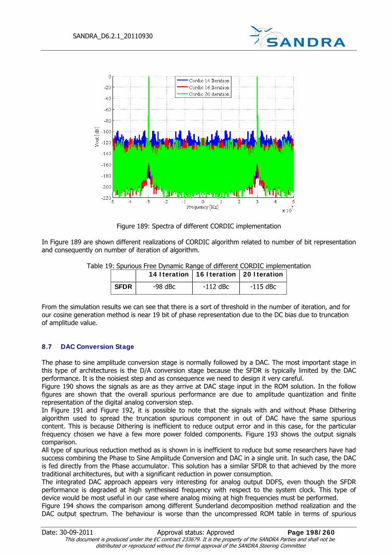
SANDRA_D6.2.1_20110930
Date: 30-09-2011 Approval status: Approved Page 198/260 This document is produced under the EC contract 233679. It is the property of the SANDRA Parties and shall not be
distributed or reproduced without the formal approval of the SANDRA Steering Committee
Figure 189: Spectra of different CORDIC implementation In Figure 189 are shown different realizations of CORDIC algorithm related to number of bit representation and consequently on number of iteration of algorithm.
Table 19: Spurious Free Dynamic Range of different CORDIC implementation 14 Iteration 16 Iteration 20 Iteration
SFDR -98 dBc -112 dBc -115 dBc
From the simulation results we can see that there is a sort of threshold in the number of iteration, and for our cosine generation method is near 19 bit of phase representation due to the DC bias due to truncation of amplitude value.
8.7 DAC Conversion Stage
The phase to sine amplitude conversion stage is normally followed by a DAC. The most important stage in this type of architectures is the D/A conversion stage because the SFDR is typically limited by the DAC performance. It is the noisiest step and as consequence we need to design it very careful. Figure 190 shows the signals as are as they arrive at DAC stage input in the ROM solution. In the follow figures are shown that the overall spurious performance are due to amplitude quantization and finite representation of the digital analog conversion step. In Figure 191 and Figure 192, it is possible to note that the signals with and without Phase Dithering algorithm used to spread the truncation spurious component in out of DAC have the same spurious content. This is because Dithering is inefficient to reduce output error and in this case, for the particular frequency chosen we have a few more power folded components. Figure 193 shows the output signals comparison. All type of spurious reduction method as is shown in is inefficient to reduce but some researchers have had success combining the Phase to Sine Amplitude Conversion and DAC in a single unit. In such case, the DAC is fed directly from the Phase accumulator. This solution has a similar SFDR to that achieved by the more traditional architectures, but with a significant reduction in power consumption. The integrated DAC approach appears very interesting for analog output DDFS, even though the SFDR performance is degraded at high synthesised frequency with respect to the system clock. This type of device would be most useful in our case where analog mixing at high frequencies must be performed. Figure 194 shows the comparison among different Sunderland decomposition method realization and the DAC output spectrum. The behaviour is worse than the uncompressed ROM table in terms of spurious

SANDRA_D6.2.1_20110930
Date: 30-09-2011 Approval status: Approved Page 199/260 This document is produced under the EC contract 233679. It is the property of the SANDRA Parties and shall not be
distributed or reproduced without the formal approval of the SANDRA Steering Committee
content but we have to remember that the level achieved can justify the more appreciable memory saving that as we have seen car be of 200:1 for 18 bit decomposition. The last figure shows a particular behaviour, as we can see that the DAC spurious contribute is relatively independent from the CORDIC solution adopted. In Table 20, we can see that the DAC spurious contribute is more high in ROM based method whereas the iterative nature of CORDIC algorithm allows a better overall behaviour with the best SFDR on the output signal.
Table 20: SFDR of different algorithms for cosine generation
ROM LUT implementation Sunderland algorithm CORDIC algorithm
SFDR -85.9 dBc -68.5 dBc -91.2 dBc
Figure 190: DAC input signal comparison
Figure 191 : LUT implementation input output signal comparison

SANDRA_D6.2.1_20110930
Date: 30-09-2011 Approval status: Approved Page 200/260 This document is produced under the EC contract 233679. It is the property of the SANDRA Parties and shall not be
distributed or reproduced without the formal approval of the SANDRA Steering Committee
Figure 192: DAC Dithered signal input output comparison
Figure 193: DAC signal output comparison
Figure 194: Different Sunderland DAC output signal comparison

SANDRA_D6.2.1_20110930
Date: 30-09-2011 Approval status: Approved Page 201/260 This document is produced under the EC contract 233679. It is the property of the SANDRA Parties and shall not be
distributed or reproduced without the formal approval of the SANDRA Steering Committee
Figure 195: Different CORDIC iteration and DAC output signal comparison
8.8 Performance Consideration and Conclusion
As demonstrated in this chapter the DDS technology with general modification on operative functioning is suitable for WiMAX and thus, also AeroMACS signal generation and its use in airport environment but as seen, a designer is faced with a wide array of choices for cosine generation step due to space and power consumption needs for the type of utilization. The ROM solutions presented can be taken in account in this condition because the high operative frequency enables a high system clock and use of faster memory to obtain lower error level. The simulations demonstrated that the proposed architectures can reach the IEEE 802.16 signal generation error performance request and this technology will allow a better cost dependent design to cover large areas and can permit a better BS location to improve the system overall performances.

SANDRA_D6.2.1_20110930
Date: 30-09-2011 Approval status: Approved Page 202/260 This document is produced under the EC contract 233679. It is the property of the SANDRA Parties and shall not be
distributed or reproduced without the formal approval of the SANDRA Steering Committee
9 AeroMACS Convergence Sub-layer The Convergence Sub-layer (CS) of the IEEE 802.16 standard specifies the interface towards higher layer protocols. The standard provides a variety of convergence sub-layer options in order to provide the possibility to interface with a versatile set of higher layer protocols. A main function of the convergence sub-layer is the acceptance and interpretation of Service Data Units (SDU) received from higher layers. Based on a manageable policy, SDUs are mapped to specific service flows. Additionally, header compression techniques or any other appropriate processing may be conducted by the convergence sub-layer protocol. The AeroMACS draft profile intends to support the IP CS (specifically IPv6), additionally the support of Ethernet is discussed. In principle the issue of the convergence sub-layer seems straight forward - either AeroMACS supports higher layer protocol A, higher layer protocol B, or even both. However, recalling the principle design issues of layered communication protocol architectures there may be problems considering the two options of the packet based convergence sub-layer, namely IP CS and Ethernet CS. The required service differs from the IP point of view and may cause problems when considering IP over AeroMACS. Using IP CS would require managing each individual connection to a mobile station as a point to point link. In contrast an Ethernet CS would model a point to multi-point link. Consequently the service offered toward IP is different.
9.1 CS Options
The Network Working Group (NWG) of the WiMAX Forum™ has defined network architecture for IEEE 802.16 sub-networks, thereby, considering topics at layers above those defined by the 802 standards. The Internet Engineering Task Force (IETF) in cooperation with the WiMAX Forum has worked out a Request For Comment (RFC) "Transmission of IPv6 via the IPv6 Convergence Sub-layer over IEEE 802.16 Networks" which provides a full conformant IPv6 connectivity through an IP point to point link. This solution fits the general business use case where each subscriber resides in its own sub-network. However, the requirements of the sub-network in an aeronautical environment might be different than the one of an ordinary business use case. Running IPv6 over AeroMACS shall be fully compliant to the IP standard, thereby; IP multicast shall be supported preferably in an efficient manner. It might also be desirable to support multicast at link layer which is difficult with point to point links. Furthermore, an RFC 5692 "Transmission of IP over Ethernet over IEEE 802.16 Networks" has been published discussing a possible way of operating IP over Ethernet over WiMAX. However, Ethernet in this case does also not support multicast at link layer. Hence, Ethernet frames that are broadcast or multicast are being replicated and then carried via unicast transport connection on the IEEE 802.15 access link. Supporting an Ethernet CS would still provide the opportunity to exploit the efficient multicast support of an Ethernet link while sitll being able to create separate sub-networks for individual aircraft. However, the additional Ethernet header would also increase the overhead via the wireless link. Dependent on the deployment and use case of AeroMACS it could be beneficial to introduce a possibility to implement a native multicast capability. However, in both cases IP or ETH CS a special non standard solution would be required to realize such a feature. Considering the additonal requirements necessary to be implemented at the ground in order to support an Ethernet based communication environment for AeorMACS, IP CS seems to be the better choice.

SANDRA_D6.2.1_20110930
Date: 30-09-2011 Approval status: Approved Page 203/260 This document is produced under the EC contract 233679. It is the property of the SANDRA Parties and shall not be
distributed or reproduced without the formal approval of the SANDRA Steering Committee
10 AeroMACS MAC Analysis The IEEE 802.16 standard specifies a point to point and connection oriented link, i.e. each SDU received from an interfacing higher layer is mapped to a unique and unidirectional service flow with specific Quality of Service (QoS) parameters. Thereby, the interfacing higher layer can be one of several different types. The MAC common part sub-layer operates in a point to multipoint environment. BS is the only user of the Downlink (DL) resources, whereas MSs have to share the Uplink (UL) resources. All Mobile Stations are able to receive DL transmissions. Based on the Connection Identifier (CID) carried within the generic MAC header of each MAC PDU a MS is able to determine whether a MAC PDU is destined to it or not. A central concept of the IEEE 802.16 standard is the usage of transport connections which allows the utilization of QoS at MAC level. Each service flow has specific QoS parameters initialized at connection setup. Thereby, different data delivery strategies can be utilized (e.g. best effort, polling, etc.). At system initialization two pairs of management connections, namely the basic connection and the primary management connection, have to be established between MS and BS. A third management connection, the secondary management connection, may be established, too. However, such a connection is only mandatory for managed "subscriber stations". In certain circumstances especially if remote airport equipment is being used such a secondary management connection would probably make sense. However, the basic management connection shall be used to transmit short and time urgent MAC management messages while the primary management connection shall be used to exchange longer and delay tolerant MAC management messages.
This chapter describes elements related to the data exchange protocol relevant to the performance of the
AeroMACS communication system.
10.1 MAC PDU Formats
The IEEE 802.16 standard offers various options for fragmenting and reassembling MAC SDUs. Thereby, a MAC SDU may be of variable or fixed length. In the case of AeroMACS a variable length of MAC SDUs shall be allowed. Generally, a MAC Protocol Data Unit (PDU) shall be of the form as depicted in Figure 196. Each MAC PDU starts with a fixed length header of 6 bytes (the generic MAC header). A MAC PDU typically contains payload and shall then be appended by a 4 bytes Cyclic Redundancy Checksum (CRC). The payload itself may further contain several sub-headers. The fragmentation sub-header is used if an entire MAC SDU does not fit into a single MAC PDU. The packing sub-header is used if several MAC SDUs are packed together into a single MAC PDU. Multiple MAC PDUs may also be concatenated during a single burst. If the MAC PDU does not contain payload data, MAC header needs no CRC as the MAC header itself contains a header checksum. The generic MAC header contains the Connection Identifier (CID) of the connection with which the PDU is associated. The MAC PDU does not contain any source or destination address in its header.

SANDRA_D6.2.1_20110930
Date: 30-09-2011 Approval status: Approved Page 204/260 This document is produced under the EC contract 233679. It is the property of the SANDRA Parties and shall not be
distributed or reproduced without the formal approval of the SANDRA Steering Committee
Figure 196: Overview of different MAC PDU options
10.2 Automatic Repeat Request
Generally, Automatic Repeat Request (ARQ) protocols are used to synchronize data flows between sending and receiving entities. Thereby, the flow control procedure takes care that the data source is not overloading the data sink. Also erroneous data packets are indicated to the source (through negative acknowledgments). The IEEE 802.16 standard offers four different types of ARQ, namely, go-back-n, selective-reject, and two combinations of go-back-n and selective-reject. Go-back-n may also be called as cumulative ARQ. An ARQ information element has at least a size of 4 byte and at most of 12 byte. The basic components of an ARQ information element are the CID field and the Block Sequence Number (BSN) field. The CID identifies the transport connection and the BSN is differently used dependent on the ARQ type.
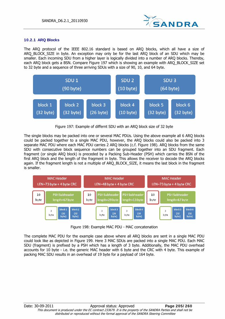
SANDRA_D6.2.1_20110930
Date: 30-09-2011 Approval status: Approved Page 205/260 This document is produced under the EC contract 233679. It is the property of the SANDRA Parties and shall not be
distributed or reproduced without the formal approval of the SANDRA Steering Committee
10.2.1 ARQ Blocks
The ARQ protocol of the IEEE 802.16 standard is based on ARQ blocks, which all have a size of ARQ_BLOCK_SIZE in byte. An exception may only be for the last ARQ block of an SDU which may be smaller. Each incoming SDU from a higher layer is logically divided into a number of ARQ blocks. Thereby, each ARQ block gets a BSN. Compare Figure 197 which is showing an example with ARQ_BLOCK_SIZE set to 32 byte and a sequence of three arriving SDUs with a size of 90, 10, and 64 byte.
Figure 197: Example of differnt SDU with an ARQ block size of 32 byte The single blocks may be packed into one or several MAC PDUs. Using the above example all 6 ARQ blocks could be packed together to a single MAC PDU, however, the ARQ blocks could also be packed into 3 separate MAC PDU where each MAC PDU carries 2 ARQ blocks (c.f. Figure 198). ARQ blocks from the same SDU with consecutive block sequence numbers can be grouped together into an SDU fragment. Each fragment (or single ARQ block) is preceded by a Packing Sub-Header (PSH) which carries the BSN of the first ARQ block and the length of the fragment in byte. This allows the receiver to decode the ARQ blocks again. If the fragment length is not a multiple of ARQ_BLOCK_SIZE, it means the last block in the fragment is smaller.
Figure 198: Example MAC PDU - MAC concatenation The complete MAC PDU for the example case above where all ARQ blocks are sent in a single MAC PDU could look like as depicted in Figure 199. Here 3 MAC SDUs are packed into a single MAC PDU. Each MAC SDU (fragment) is prefixed by a PSH which has a length of 3 byte. Additionally, the MAC PDU overhead accounts for 10 byte - i.e. the generic MAC header with 6 byte and the CRC with 4 byte. This example of packing MAC SDU results in an overhead of 19 byte for a payload of 164 byte.

SANDRA_D6.2.1_20110930
Date: 30-09-2011 Approval status: Approved Page 206/260 This document is produced under the EC contract 233679. It is the property of the SANDRA Parties and shall not be
distributed or reproduced without the formal approval of the SANDRA Steering Committee
Figure 199: Example MAC PDU - MAC packing
10.2.2 ARQ Feedback
After transmitting a block, the transmitter waits for a time of ARQ_RETRY_TIMEOUT for the arrival of an acknowledgment from the receiver. After that the block is resent a window of BSNs is maintained which spans from the first BSN of a block which has not been acknowledged yet to the last such BSN. When a block with the BSN of the window start is received, the window start is advanced. The receiver can send positive as well as negative acknowledgments about the blocks it has or has not received. It keeps a window of BSNs from the first BSN of a block which has been received to the last such block. When all BSNs belonging to an SDU are received that SDU is passed on to the upper layer and the BSNs are marked as received, with the window start updated accordingly.
10.2.2.1 ACK Type 0 (Selective ACK entry) and ACK Type 2 (Cumulative with Selective ACK entry)
The BSN corresponds to the first bit in the ACK Map. The ACK Maps span from 16 to 48 bits corresponding to the BSN and the succeeding BSNs. Each bit set to 1 indicates a positive acknowledgment. If ACK Type is 2 instead of 0 then the first bit must be set to 1 and the BSN is interpreted as a cumulative ACK, with the remaining bits indicating selective ACKs like with type 0. For example to acknowledge all blocks up to 1010 and then blocks 1012 and 1015, the BSN could be set to 1010 and the ACK Map could be set to binary 1010010000000000. The same could be achieved by setting the BSN to 1000 and the ACK Map to binary 111111111101001. The difference is that in the first case there are negative acknowledgments for blocks 1016 up to 1025 inclusive which may not be wanted. In the second case the 1-bits for BSNs 1000 to 1009 do not matter on the other hand as the intention was to acknowledge all BSNs up to 1010 anyway.
Table 21: MAC header informational elements of ARQ Type 0 or ARQ Type 2 CID 16 (bit) LAST 1 (bit) ACK Type=0 or 2 2 (bit) BSN 11 (bit) n=Number of ACK Maps 2 (bit) n+1 times Selective ACK Map 16 (bit) Total size 48/64/80/96 (bits)
10.2.2.2 ACK Type 1 (Cumulative ACK entry)
The BSN is a cumulative ACK entry. All blocks up to and including this BSN are acknowledged as having been received.

SANDRA_D6.2.1_20110930
Date: 30-09-2011 Approval status: Approved Page 207/260 This document is produced under the EC contract 233679. It is the property of the SANDRA Parties and shall not be
distributed or reproduced without the formal approval of the SANDRA Steering Committee
Table 22: MAC header informational elements of ARQ Type 1 CID 16 (bit)LAST 1(bit) ACK Type=1 2 (bit) BSN 11 (bit)reserved=0 2 (bit) Total size 32 (bit)
10.2.2.3 ACK Type 3 (Cumulative ACK with Block Sequence ACK entry)
Table 23: MAC header informational elements of ARQ Type 3
CID 16 (bit) LAST 1 (bit) ACK Type=3 2 (bit) BSN 11 (bit) n=Number of ACK Maps 2 (bit) n+1 times Sequence Format 1 (bit)
Sequence ACK MapSequence Lengths 15 (bit)
Total size 48/64/80/96 (bit)
The BSN is a cumulative ACK entry, like with type 1 and 2. In addition a number of block sequences is present. There are 1 to 4 maps with each either containing two sequences with the lengths given in 6 bit or three sequences with the lengths given in 4 bit. Each sequence specifies a number of consecutive BSN entries, with the first sequence starting at the cumulative BSN plus one. (Which is always a NACK, otherwise the cumulative BSN could be increased by one.) The Sequence ACK Map specifies if each sequence contains positive or negative acknowledgment of the contained BSNs. For example to acknowledge all blocks up to and including BSN 1000 and then BSNs 1020 to 1025, 1030 to 1050 and 1070 and 1071 the IE could look like this:
Table 24: Example CID LAST ACK Type 3 BSN 1000 n=Number of ACK Maps 2 Map 1 Sequence Format 0
Sequence ACK MapSequence Lengths
01 binary 19, 6
Map 2 Sequence Format 0 Sequence ACK MapSequence Lengths
01 binary 4, 21
Map 3 Sequence Format 0 Sequence ACK MapSequence Lengths
01 binary 19, 2
Total size 48/64/80/96

SANDRA_D6.2.1_20110930
Date: 30-09-2011 Approval status: Approved Page 208/260 This document is produced under the EC contract 233679. It is the property of the SANDRA Parties and shall not be
distributed or reproduced without the formal approval of the SANDRA Steering Committee
The first map starts at BSN+1 which is 1001. The start of the other 5 maps is found by adding the lengths of the previous maps, so they start at 1020, 1026, 1030, 1051, 1070.
10.2.3 Quality of Service (QoS)
Quality of Service in IEEE 802.16 is supported through the concept of unicast transport connections. These transport connections are called service flows, where each service flow utilizes a particular set of QoS parameters. The standard provides several QoS parameters to be adjusted; for instance maximum sustained traffic rate, maximum traffic burst, minimum reserved traffic rate, maximum latency, etc. - in principle latency, jitter, and throughput assurance. Service flows are either provisioned or dynamically added by the base station or optionally by the mobile station. How to provision service flows is out of the scope of the IEEE 802.16 standard, consequently it is also not specified in the AeroMACS draft profile. Certain service flows may be added dynamically for instance after the network entry procedure. The standard provides options to create, change, and delete a service flow dynamically. Such procedures can be either initiated by the base station or by the mobile station. The WiMAX mobile profile makes these options mandatory to be supported by the base station. The capability to dynamically create or change a service flow is optional for a mobile station; however, the deletion of a service flow is mandatory. The AeroMACS profile intends to support only the dynamic service flow creation, change, and deletion procedures to be initiated by the base station. How these service flows are initiated and / or triggered is not specified by the AeroMACS profile. QoS parameters of ATC traffic flows shall probably be regulated while QoS parameters of AOC traffic flows may be provider dependent.
10.2.4 Data Delivery Service
There are different possibilities to provide bandwidth to a mobile station, realized through a scheduling service. Uplink request and grant scheduling is performed by the base station in order to provide each MS with bandwidth for uplink transmissions or opportunities to request bandwidth. By specifying a scheduling type and its associated QoS parameters, the BS scheduler can anticipate the throughput and latency needs for the uplink traffic and provide polls and/or grants at the appropriate times. The different scheduling services are:
• Unsolicited Grant Service (UGS)
• real-time Polling Service (rtPS)
• non-real-time Polling Service (nrtPS)
• Best Effort (BE)
The unsolicited grant service is intended for real-time applications which generate fixed-rate data. Among others QoS parameters such as tolerated jitter, minimum reserved traffic rate, maximum latency, and the unsolicited grant interval are defined. This means that a service flow with a data delivery service of UGS gets periodically UL resources assigned without requesting them each time.
Figure 200: The Unsolicited Grant Service usable for uplink transmissions

SANDRA_D6.2.1_20110930
Date: 30-09-2011 Approval status: Approved Page 209/260 This document is produced under the EC contract 233679. It is the property of the SANDRA Parties and shall not be
distributed or reproduced without the formal approval of the SANDRA Steering Committee
The real-time Polling service (rtPS) is intended for real time applications with variable bit rates. Among others QoS parameters such as maximum latency, minimum reserved traffic rate, traffic priority, and the polling interval are defined. In this case the resource scheduler polls a mobile station regularly at fixed intervals. These polls may be used to request bandwidth.
Figure 201: The real-time Polling service usable for uplink transmissions
The non-real-time Polling Service (nrtPS) is intended for applications which require guaranteed data rate but are insensitive to delays. QoS parameters such as minimum reserved traffic rate, maximum sustained traffic rate, and traffic priority are defined. In this case the unicast polls are issued at a variable interval length (dependent on the available resources). The polls may be used to request bandwidth.
Figure 202: The non-real-time Polling Service usable for uplink transmissions
The Best Effort service is intended for applications with no rate or delay requirements. In this case bandwidth request ranging opportunities are provided to transmit bandwidth request ranging codes. If a bandwidth request range code is successfully received by a base station it polls the associated mobile station.
Figure 203: The Best Effort service usable for uplink transmissions
For the downlink direction similar QoS classes can be utilized. However, these are called slightly different but have comparable QoS parameters. The scheduler does not need to consider any polls or ranging opportunities for the downlink, though. The different QoS classes or data delivery services are:

SANDRA_D6.2.1_20110930
Date: 30-09-2011 Approval status: Approved Page 210/260 This document is produced under the EC contract 233679. It is the property of the SANDRA Parties and shall not be
distributed or reproduced without the formal approval of the SANDRA Steering Committee
• UGS
• Real-Time Variable Rate (RT-VR) service
• Non-Real-Time Variable Rate (NRT-VR) service
• BE service
What kind of QoS class a specific application or set of applications will require is dependent on the requirements. How the different data delivery services and scheduling strategies are implemented is not specified by the standard. Thus, they are vendor dependent. In any case the communication service provider has to assure that safety related communication is preferred over non safety related communication. It might be that a simple priority scheme with a best effort service is sufficient.
10.2.5 Request Grant Mechanisms
A mobile station is required to support at least three different connections. That is, two management connections which are set up at network entry and one data bearer to transmit user data. Every connection with a QoS service other than UGS needs to adapt its resource requirements. This is done through bandwidth requests. This is a mechanism where a mobile station indicates to the base station that it requires uplink resources. Bandwidth requests are either sent as standalone Bandwidth Request (BR) headers or as a Piggy Back Request (i.e. included in the Grant Management Sub-Header (GMSH)). Bandwidth Requests may be either incremental or aggregated. When a BS receives an incremental BR, it shall add the quantity of bandwidth requested to its current perception of the bandwidth needs of the connection. When the BS receives an aggregate BR, it shall replace its perception of the bandwidth needs of the connection with the quantity of bandwidth requests. Piggybacked bandwidth requests are always incremental. The base station issues resource grants towards a mobile station based on the basic CID (i.e. basic management connection). This means that a mobile station is able to utilize the concept of bandwidth stealing where a certain amount of requested bandwidth for a specific QoS class may be utilized differently. However, the resource requests are based on the transport connection which requires bandwidth. If a base station polls a mobile station, it typically assigns enough resources to issue a bandwidth request.

SANDRA_D6.2.1_20110930
Date: 30-09-2011 Approval status: Approved Page 211/260 This document is produced under the EC contract 233679. It is the property of the SANDRA Parties and shall not be
distributed or reproduced without the formal approval of the SANDRA Steering Committee
11 Simulations This chapter presents results of the joint activity of SANDRA SP6 WP6.2 and SJU WP15.2.7 of the AeroMACS data traffic modeling and load analysis. It discusses traffic models, simulation scenarios, and respective results. Furthermore, AeroMACS MAC simulations related to data exchange have been conducted. The various scenarios and results are presented within this chapter. In order to assess the performance of AeroMACS properly an assumption on the data traffic load was necessary. The data traffic load model proposed here was used as input for the AeroMACS communication profile definition. Thereby, the airport data load model describes the characteristics of the envisaged Air Traffic Control (ATC), Aeronautical Operational Control (AOC), and Network management (NET) services as anticipated by [COCR]. In order to simulate this model the following inputs were necessary:
• Air traffic model: This is the simulation of the aircraft movement on the airport. Departing aircraft moving from ramp to runway, arriving aircraft moving from runway to ramp, and ground vehicles.
• Supported applications: This are the data link applications envisaged for the airport domain and their trigger events. Note that most aeronautical data link applications are triggered by events related to the progress of the flight. The events are provided by the air traffic model.
• Scenarios: These are the different use cases of the airport data link. This relates mostly to the amount of aircraft serviced, and the various sets of supported applications.
The output of the data traffic model is the statistical description of the expected offered load at application layer (ISO/OSI layer 7). The offered load is the amount of data produced by the applications – this does not include any overhead of the transport layer, network layer, or data link layer. In addition to the statistical description, the data traffic model is also provided as a XML file to support the further utilization of the data – for instance as input (i.e. load generator) for protocol simulations.
11.1 Traffic Models
The data model described within this document shall reflect the characteristics of the used ATC applications, AOC applications, and NET traffic applications for aircraft and ground vehicles located at an airport. Input for this estimation has been taken from [COCR] and [WOO_10]. The gained results are based on different inputs, namely:
• the mobility model for aircraft,
• the mobility model for ground vehicles,
• the supported applications, and
• the different scenarios.
The mobility models for aircraft (i.e. moving aircraft) and ground vehicles are necessary in order to distribute the produced data traffic over time. Additionally, certain ATC and AOC applications have an order of events and are utilized only in certain positions (i.e. RAMP, GROUND, TOWER - compare next sub-chapter). The supported set of applications and their trigger events is necessary to associate an application with a certain time window. Furthermore, different scenarios shall allow a sensitivity analysis of the average offered load. The output of the data traffic model is a statistical description of the average offered load at application layer (ISO/OSI layer 7). Offered load is the amount of data solely produced by applications – this does not include any overhead which might be caused by a Transport Layer, Network Layer, or the Data Link Layer itself. However, [COCR] considers an overhead of 77 or 78 byte (assuming an ATN stack), which is also reflected within the presented results.

SANDRA_D6.2.1_20110930
Date: 30-09-2011 Approval status: Approved Page 212/260 This document is produced under the EC contract 233679. It is the property of the SANDRA Parties and shall not be
distributed or reproduced without the formal approval of the SANDRA Steering Committee
11.1.1 Airtraffic Model
Within the model an aircraft traverses the following positions when departing from an airport and arriving at an airport, respectively:
• RAMP
• GROUND
• TOWER
Thereby, RAMP denotes the time an aircraft stays at the gate before departure; GROUND denotes the time from push back until the time of taxiing to the runway is completed; TOWER denotes the time after control is handed over from ground to tower until take-off. Thereby, take-off is NOT included as the airport communication system will not support high speeds. Typical dwell times of an aircraft in the respective zones were taken from [COCR]. Note that [COCR] distinguishes between two phases (i.e. Phase 1 and Phase 2). Where the first phase (Phase 1) is based on existing or emerging data communications services and completes around 2020. The second phase (Phase 2) represents a new paradigm in the use of data communication. Data communications services are introduced that replace or supplement those in Phase 1, and data communications is the primary means of air-ground communication. Data communications supports increased automation in the aircraft and on the ground. A fully operational Phase 2 concept is anticipated for the year 2030. Note that for this evaluation only Phase 2 has been assumed. Table 25 shows the different average dwell times of an aircraft within a given position (i.e. RAMP, GROUND, or TOWER). [COCR] further distinguishes between an high density (HD) airport and a low density (LD) airport. The dwell times in the respective positions are also different for arriving aircraft (ARR) and departing aircraft (DEP). Within this evaluation only high density airports were considered.
Table 25: Aircraft dwell times in different positions (Source: Table 6-5, page 102 of [COCR])
APT domain RAMP GROUND TOWER P2-HD DEP 1800 sec [30 min] 720 sec [12 min] 270 sec [4.5 min]P2-HD ARR 360 sec [6 min] 480 sec [8 min] 270 sec [4.5 min]P2-LD DEP 900 sec [15 min] + 360 sec [6 min] = 1260 sec [21 min] 150 sec [2.5 min]P2-LD ARR 180 sec [3 min] + 240 sec [4 min] = 420 sec [7 min] 150 sec [2.5 min]
The intention of this work was the creation of aircraft mobility models with a given average amount of aircraft. Assuming the amount of aircraft in a scenario is N, then a certain amount of aircraft (A/C) is departing (D) and arriving (A). These models apply
N = x*A + y*D (Little's Law) (Eq.339) with
• A - arrival process length (in seconds) - should be a Uniform Distribution +/- 10% of the mean
value.
• A_HD = 360 sec + 480 sec + 270 sec = 1110 sec (Phase 2 High Density)
• D - departure process length (in seconds) - should be a Uniform Distribution +/- 10% of the mean
value.
• D_HD = 1800 sec + 720 sec + 270 sec = 2790 sec (Phase 2 High Density)
• X - A/C arrival rate (x/sec).
• Y - A/C departure rate (y/sec).
• N - A/C on airport

SANDRA_D6.2.1_20110930
Date: 30-09-2011 Approval status: Approved Page 213/260 This document is produced under the EC contract 233679. It is the property of the SANDRA Parties and shall not be
distributed or reproduced without the formal approval of the SANDRA Steering Committee
Now the assumption of a more or less constant number N of aircraft within the simulation of the airport scenario holds. The equation (Eq.339) has two unknowns, namely x and y. Therefore, we have to assume a relationship between x and y (e.g. x == y, 2x == y, etc.), in order to get the arrival rates for both. Table 26 and Table 27 show values used for the different scenarios. The first column indicates the average number of simulated aircraft within a scenario. The second column shows the relationship of the arrival rate of arriving aircraft x and the arrival rate of departing aircraft y. The third and fourth columns indicate the calculated arrival and departure rates of aircraft per second, respectively. And the fifth and sixth columns show the average number of simulated aircraft for arrivals and departures, respectively.
Table 26: Arrival Scenarios
Number of aircraft Y == ?*X
Arrival Rate X
DepartureRate Y
Simulated Arrivals
Simulated Departures
1 0,2 0,0006 0,0001 0,67 0,33 10 0,2 0,0060 0,0012 6,65 3,35 15 0,2 0,0090 0,0018 9,98 5,02 20 0,2 0,0120 0,0024 13,31 6,69 25 0,2 0,0150 0,0030 16,64 8,36 30 0,2 0,0180 0,0036 19,96 10,04 50 0,2 0,0300 0,0060 33,27 16,73 100 0,2 0,0600 0,0120 66,55 33,45 200 0,2 0,1199 0,0240 133,09 66,91
The mobility scenarios have been chosen in such a way that either more aircraft are arriving than departing and vice versa. The proportion is roughly 2/3 to 1/3. The derived arrival and departure rates are used as input for an exponential distribution in order to model the aircraft arrival processes. In total two arrival processes were implemented one for arriving aircraft and one for departing aircraft.
Table 27: Departure Scenarios Number of aircraft Y == ?*X
Arrival Rate X
Departure Rate Y
Simulated Arrivals
Simulated Departures
1 1 0,0003 0,0003 0,28 0,72 10 1 0,0026 0,0026 2,85 7,15 15 1 0,0038 0,0038 4,27 10,73 20 1 0,0051 0,0051 5,69 14,31 25 1 0,0064 0,0064 7,12 17,88 30 1 0,0077 0,0077 8,54 21,46 50 1 0,0128 0,0128 14,23 35,77 100 1 0,0256 0,0256 28,46 71,54 200 1 0,0513 0,0513 56,92 143,08
11.1.2 Ground Vehicle Traffic Model
A similar approach has been used for the mobility model of ground vehicles. The average vehicle dwell time has been modeled to be roughly 1800 second per instance. 75 % of this time a ground vehicle stays in the RAMP area and 25 % of this time it stays in the GROUND are. Vehicles are not regarded in the TOWER area. The dwell time in this case can be seen more as a time window where vehicles may use certain data applications.

SANDRA_D6.2.1_20110930
Date: 30-09-2011 Approval status: Approved Page 214/260 This document is produced under the EC contract 233679. It is the property of the SANDRA Parties and shall not be
distributed or reproduced without the formal approval of the SANDRA Steering Committee
Table 28: Vehicle Scenarios
Number of vehicles Average dwell time Arrival rate
1 1800 0,0006 4 1800 0,0022 6 1800 0,0033 8 1800 0,0044 10 1800 0,0056 20 1800 0,0111 40 1800 0,0222
11.1.3 Application Modeling and Mapping
The data traffic model consists of several applications, where each application has individual characteristics. A specific air traffic application may be used several times during the duration of a flight. It may be used never, too. In general a service is triggered for a given period of time. It is important to note that each trigger is a combination of an event (e.g. moving from RAMP to GROUND) and the duration of the flight phase until the next trigger event (e.g. residing at the ramp until push-back is initiated). Within this context we call the triggering event plus the trigger duration of an application instance (see Figure 204).
Figure 204: Possible application instance trigger events during a flight An application instance contains of 1 to n dialogues, where a dialogue may consist of 0 to f FL messages and 0 to r RL messages. An aeronautical data communication service may start its dialogues within a service instance either at the beginning, at the end, or (in absence of a specification) at a random point during the service instance duration (Figure 205). If a service instance consists of more than one dialogue the dialogues are evenly distributed with a random offset (up to +/-10% of the service instance duration).

SANDRA_D6.2.1_20110930
Date: 30-09-2011 Approval status: Approved Page 215/260 This document is produced under the EC contract 233679. It is the property of the SANDRA Parties and shall not be
distributed or reproduced without the formal approval of the SANDRA Steering Committee
Figure 205: Application instance consists of dialogues
FL and RL messages may be separated by the Human Interaction Time (HIT) (if applicable) and the Required Communication Technical Performance (RCTP) one way latency. The RCTP is the required 95% percentile latency of any aeronautical data link technology, specified in [COCR]. The maximum execution time is calculated through the separation time of consecutive FL and RL messages. This interval time is calculated through the RCTP one way latency and (if applicable) HIT multiplied by two (Figure 206). This models an interactive application data exchange (i.e. a message and a response) performed over a data link technology providing the minimum latency requirements specified in [COCR] (i.e. which are defined by the RCTP). The human interaction time is only included if the application message generation is human dependent.
Figure 206: Message separation times within a single dialogue
In total 16 ATC services, 43 AOC services, and 2 NET services for aircraft were modeled. Additionally, 7 AOC services for vehicles were considered. Aircraft trigger different applications dependent on whether an aircraft is arriving or departing and on the aircraft's current position (i.e. RAMP, GROUND; TOWER). Not every aircraft triggers all applications as certain applications are equipment dependent or are used only in certain update cycles (for instance the AOC E-CHARTS application). Vehicles trigger applications which are mapped to a specific position (compare Table 29). Departing aircraft may trigger 13 ATC services and 35 AOC services while residing at the RAMP position; 4 ATC services and 2 NET services while moving at the GROUND position; and 2 ATC services and 2 AOC services within the TOWER position. Arriving aircraft may trigger 1 ATC service and 6 AOC services while residing at the RAMP position, 4 ATC services and 5 AOC services while moving within the GROUND position; and 2 ATC services and 2 AOC services within the TOWER position. Vehicles may trigger 6 AOC services while residing in the RAMP position and 7 AOC services while moving within the GROUND position. Table 29 gives an overview of the different applications and their mapping to the various positions. It clearly shows that most applications are triggered for aircraft which are residing at the RAMP position and which are preparing their flight (i.e. which are departing). Data intensive applications are the AOC applications "Electronic Flight Folder Exchange (EFF)", "Electronic Library Update (UPLIB)", and "E-CHARTS". Also the "Flight Journal Documentation (FLTJOURNAL)" and "Flight Operational Quality Assurance (FOQA)" contribute significantly to the offered load.

SANDRA_D6.2.1_20110930
Date: 30-09-2011 Approval status: Approved Page 216/260 This document is produced under the EC contract 233679. It is the property of the SANDRA Parties and shall not be
distributed or reproduced without the formal approval of the SANDRA Steering Committee
Table 29: Mapping of application to appropriate positions RAMP GROUND TOWER
DEPARTURE ARRIVAL DEPARTURE ARRIVAL DEPARTURE ARRIVAL
ATC ACM, COTRAC
(interactive), COTRAC
(wilco), DCL, D-FLUP,
DLL, D-OTIS, D-RVR,
D-SIG, D-SIGMENT,
FLIPCY, FLIPINT, PPD
ACM ATC, ACM,
D-TAXI,
SURV
ACL, ACM,
D-TAXI,
SURV
ACM, SURV ACM, SURV
AOC AOCDLL, FLTPLAN,
LOADSHT, OOOI,
SWLOAD, TECHLOG,
UPLIB, WXGRAPH,
WXTEXT, BRFCD,
DOOR, ACLOG,
AIRWORTH, BAGGAGE,
NOTAM, CATERING,
DEICING, CREW-L,
CREW-RPS, CREW-BUL,
EFF, EFFU, E-BILL, E-
CHARTS, CREW-REG,
FLOWCON, FOQA,
HANDLING, LOADDOC,
NOTOC, PASSENGER,
PREFLT-INS,
SWLOAD25, SWCONF,
TAKEOFF-CALC
CABINLOG,
FLTLOG,
OOOI,
SWLOAD,
ETS-
REPORT,
REFUEL,
N/A TECHLOG,
EFFU,
CREW-TIME,
FLTJOURNAL,
FOQA
OOOI,
WXRT
OOOI,
AUTOLAND-
REG
NET N/A N/A NETCONN,
NETKEEP
N/A N/A N/A
VC V-PLAN, DV-ALERT, AOPCL, ADLI,
DMSG, BWTI
V-PLAN, DV-ALERT,
DS-ALERT, AOPCL,
ADLI, DMSG, BWTI
N/A
11.2 Simulation Scenarios
Table 30 shows the 32 simulation scenarios which have been derived in order to show the different data traffic appearances. One group of scenarios considers the overall airport region and the other group of scenarios considers a single cell only. In the first group of scenarios the average number of aircraft N in the aircraft traffic model was 50, 100, and 200. The different positions of RAMP, GROUND, and TOWER were

SANDRA_D6.2.1_20110930
Date: 30-09-2011 Approval status: Approved Page 217/260 This document is produced under the EC contract 233679. It is the property of the SANDRA Parties and shall not be
distributed or reproduced without the formal approval of the SANDRA Steering Committee
considered separately. There are always pairs of simulation scenarios where one denotes the arrival scenario and one the departure scenario. In the arrival scenario more aircraft are arriving than departing and vice versa. Aircraft and vehicle were simulated according to the model described above, however data applications were only generated for the respective position (i.e. RAMP, GROUND, or TOWER). The average amount of vehicles for the first group of scenarios was 10, 20, and 40. For vehicles there is no difference between an arrival or departure scenario. The second group of scenarios considered the single cell situation. Different amounts of aircraft and vehicles were considered mainly for the RAMP position. For the GROUND and TOWER positions 25 aircraft and 10 ground vehicles for the single cell scenario were modeled. This makes sense as the radio coverage of GROUND and TOWER position cells have to be larger than RAMP position cells. ATC applications are not data intensive therefore all ATC applications were considered within the scenarios. Since certain AOC applications are quite data intensive, some of the scenarios did not include all AOC applications. These AOC applications were the Electronic Flight Folder Exchange (EFF) application, the Update Electronic Library (UPLIB) application, and the E-CHARTS application. The EFF application is modeled with application data messages of 2 megabyte for the download direction (aircraft to ground) and 10 megabyte for the upload direction (ground to aircraft). The EFF application is only triggered for aircraft which are preparing their flight at the RAMP position. The UPLIB application is modeled with an application data message of 40 megabyte for the upload direction. This application is triggered only by 10% of all simulated aircraft which are preparing their flight at the RAMP position. The E-CHARTS application is modeled with an application data message of 150 megabyte for the upload direction. The E-CHARTS application is triggered by 1% of all simulated departing aircraft at the RAMP position. The simulation duration was 4 hours for all scenarios where effectively 60 % of the time were evaluated (i.e. 20 % at the beginning and end of the simulation were not considered in order to avoid simulation artifacts). The evaluated figures in the subsequent chapters represent cumulated samples over the simulated time, where the sample size was 1 second. NOTE: ATC surveillance is included for all scenarios. The surveillance application is only triggered at the GROUND and TOWER positions.
Table 30: Set of simulation scenarios
# Scenario Name ~A/C ~VC Airport AreaSet of Services
AOC EFF UPLIB E-CHARTS1 HD_Phase2_50_RAMP_ARRIVAL 50 10 RAMP_ARR 2 HD_Phase2_50_RAMP_DEPARTURE 50 10 RAMP_DEP 3 HD_Phase2_50_GND_ARRIVAL 50 10 GND_ARR X 4 HD_Phase2_50_GND_DEPARTURE 50 10 GND_DEP X 5 HD_Phase2_50_TWR_ARRIVAL 50 10 TWR_ARR X 6 HD_Phase2_50_TWR_DEPARTURE 50 10 TWR_DEP X 7 HD_Phase2_100_RAMP_ARRIVAL 100 20 RAMP_ARR X 8 HD_Phase2_100_RAMP_DEPARTURE 100 20 RAMP_DEP X 9 HD_Phase2_100_GND_ARRIVAL 100 20 GND_ARR X 10 HD_Phase2_100_GND_DEPARTURE 100 20 GND_DEP X 11 HD_Phase2_100_TWR_ARRIVAL 100 20 TWR_ARR X 12 HD_Phase2_100_TWR_DEPARTURE 100 20 TWR_DEP X 13 HD_Phase2_200_RAMP_ARRIVAL 200 40 RAMP_ARR X 14 HD_Phase2_200_RAMP_DEPARTURE 200 40 RAMP_DEP X X X X 15 HD_Phase2_200_GND_ARRIVAL 200 40 GND_ARR X 16 HD_Phase2_200_GND_DEPARTURE 200 40 GND_DEP X 17 HD_Phase2_200_TWR_ARRIVAL 200 40 TWR_ARR X 18 HD_Phase2_200_TWR_DEPARTURE 200 40 TWR_DEP X 19 1CELL_1_RAMP_ARRIVAL 1 1 RAMP_ARR X 20 1CELL_1_RAMP_DEPARTURE 1 1 RAMP_DEP X X X X

SANDRA_D6.2.1_20110930
Date: 30-09-2011 Approval status: Approved Page 218/260 This document is produced under the EC contract 233679. It is the property of the SANDRA Parties and shall not be
distributed or reproduced without the formal approval of the SANDRA Steering Committee
# Scenario Name ~A/C ~VC Airport AreaSet of Services
AOC EFF UPLIB E-CHARTS21 1CELL_10_RAMP_ARRIVAL 10 4 RAMP_ARR X 22 1CELL_10_RAMP_DEPARTURE 10 4 RAMP_DEP X X X X 23 1CELL_15_RAMP_ARRIVAL 15 6 RAMP_ARR X 24 1CELL_15_RAMP_DEPARTURE 15 6 RAMP_DEP X X X X 25 1CELL_20_RAMP_ARRIVAL 20 8 RAMP_ARR X 26 1CELL_20_RAMP_DEPARTURE 20 8 RAMP_DEP X X X X 27 1CELL_25_RAMP_ARRIVAL 25 10 RAMP_ARR X 28 1CELL_25_RAMP_DEPARTURE 25 10 RAMP_DEP X X X X 29 1CELL_25_GND_ARRIVALS 25 10 GND_ARR X 30 1CELL_25_GND_DEPARTURES 25 10 GND_DEP X 31 1CELL_25_TWR_ARRIVALS 25 10 TWR_ARR X 32 1CELL_25_TWR_DEPARTURES 25 10 TWR_DEP X
11.3 Results
Table 31 and Table 32 summarize the results of all scenarios. The tables show the average offered load in kilobits per second for ATS applications and AOC applications. The considerably high variation of the offered load is discussed within this chapter.
Table 31: Average offered load for ATC and AOC applications - airport region Scenario Average offered
load ATC (Kbits/sec)
Average offered
load AOC (Kbits/sec)
Scenario 01 (50 A/C, 10 VC) RAMP arrival no A/C AOC
Overall 1,06 0,51 FL 0,43 0,42 RL 0,62 0,10
Scenario 02 (50 A/C, 10 VC) RAMP departure no A/C AOC
Overall 1,92 0,48 FL 0,78 0,39 RL 1,15 0,09
Scenario 03 (50 A/C, 10 VC) GROUND arrival service exempted
Overall 2,18 21105,04 (~21 MBit) FL 2,02 350,45 RL 0,16 20754,6
Scenario 04 (50 A/C, 10 VC) GROUND departure service exempted
Overall 2,15 11153,57 (~11 MBit) FL 2,01 178,92 RL 0,14 10975,6
Scenario 05 TOWER arrival services exempted
Overall 1,11 279,11 FL 1,08 0,0 RL 0,03 279,18
Scenario 06 (50 A/C, 10 VC) TOWER departure services exempted
Overall 0,9 596,1 FL 0,88 0,0 RL 0,02 596,1
Scenario 07 (100 A/C, 20 VC) RAMP arrival services exempted
Overall 1,91 311,27 FL 0,78 274,27 RL 1,14 37,05
Scenario 08 (100 A/C, 20 VC) RAMP departure services exempted
Overall 3,20 471,62 FL 1,29 408,09 RL 1,91 63,53
Scenario 09 (100 A/C, 20 VC) GROUND arrival
Overall 4,53 43608,33 (~43 MBit) FL 4,19 710,03

SANDRA_D6.2.1_20110930
Date: 30-09-2011 Approval status: Approved Page 219/260 This document is produced under the EC contract 233679. It is the property of the SANDRA Parties and shall not be
distributed or reproduced without the formal approval of the SANDRA Steering Committee
Scenario Average offered
load ATC (Kbits/sec)
Average offered
load AOC (Kbits/sec)
services exempted RL 0,34 42898,30 Scenario 10 (100 A/C, 20 VC) GROUND departure services exempted
Overall 3,52 18976,7 (~19 MBit) FL 3,28 312,77 RL 0,24 18665,55
Scenario 11 (100 A/C, 20 VC) TOWER arrival services exempted
Overall 2,17 538,39 FL 2,11 0,0 RL 0,06 538,39
Scenario 12 (100 A/C, 20 VC) TOWER departure services exempted
Overall 1,55 1019,44 (~1 MBit) FL 1,51 0,0 RL 0,04 1019,44
Scenario 13 (200 A/C, 40 VC) RAMP arrival all
Overall 3,0 475,49 FL 1,2 415,98 RL 1,81 59,51
Scenario 14 (200 A/C, 40 VC) RAMP departure all
Overall 6,06 14312,19 (~14 MBit) FL 2,44 12344,90 RL 3,62 1967,29
Scenario 15 (200 A/C, 40 VC) GROUND arrival all
Overall 8,98 91467,77 (~91,5 MBit)FL 8,30 1489,78 RL 0,68 89985,80
Scenario 16 (200 A/C, 40 VC) GROUND departure all
Overall 6,75 35476,70 (~35,5 MBit)FL 6,29 586,90 RL 0,46 34889,80
Scenario 17 (200 A/C, 40 VC) TOWER arrival all
Overall 4,39 960,08 (~0,9 MBit) FL 4,28 0,0 RL 0,11 960,08
Scenario 18 (200 A/C, 40 VC) TOWER departure all
Overall 2,96 1933,09 (~1,9 MBit) FL 2,89 0,0 RL 0,08 1933,09
Table 32: Average offered load for ATC and AOC applications - single cell scenario Scenario Average offered
load ATC (Kbits/sec)
Average offered
load AOC (Kbits/sec)
Scenario 19 (1 A/C, 1 VC) RAMP arrival services exempted
Overall 0,0 0,23 FL 0,0 022 RL 0,0 0,01
Scenario 20 (1 A/C, 1 VC) RAMP departure
Overall 0,04 56,69 FL 0,02 47,64 RL 0,02 9,35
Scenario 21 (10 A/C, 4 VC) RAMP arrival services exempted
Overall 0,14 20,71 FL 0,06 18,32 RL 0,08 2,43
Scenario 22 (10 A/C, 4 VC) RAMP departure
Overall 0,41 1039,82 (~1 MBit) FL 0,16 902,07 RL 0,24 139,24
Scenario 23 (15 A/C, 6 VC) RAMP arrival services exempted
Overall 0,31 52,66 FL 0,12 46,34 RL 0,18 6,32
Scenario 24 (15 A/C, 6 VC) Overall 0,66 1448,01 (~1,4 MBit)

SANDRA_D6.2.1_20110930
Date: 30-09-2011 Approval status: Approved Page 220/260 This document is produced under the EC contract 233679. It is the property of the SANDRA Parties and shall not be
distributed or reproduced without the formal approval of the SANDRA Steering Committee
Scenario Average offered
load ATC (Kbits/sec)
Average offered
load AOC (Kbits/sec)
RAMP departure
FL 0,27 1232,34 RL 0,39 215,77
Scenario 25 (20 A/C, 8 VC) RAMP arrival services exempted
Overall 0,40 74,78 FL 0,16 66,31 RL 0,24 8,48
Scenario 26 (20 A/C, 8 VC) RAMP departure
Overall 0,84 1867,43 (~1,8 MBit) FL 0,34 1619,49 RL 0,50 248,22
Scenario 27 (25 A/C, 10 VC) RAMP arrival services exempted
Overall 0,47 79,26 FL 0,19 69,42 RL 0,28 9,84
Scenario 28 (25 A/C, 10 VC) RAMP departure
Overall 1,02 2317,97 (~2,3 MBit) FL 0,41 1992,86 RL 0,60 325,45
Scenario 29 (25 A/C, 10 VC) GROUND arrival
Overall 1,23 12262,15 (~12 MBit)FL 1,14 196,97 RL 0,09 12066,22
Scenario 30 (25 A/C, 10 VC) GROUND departure
Overall 1,05 5833,0 (~5,8 MBit) FL 0,98 95,58 RL 0,07 5737,92
Scenario 31 (25 A/C, 10 VC) TOWER arrival
Overall 0,58 141,97 FL 0,57 0,0 RL 0,02 141,97
Scenario 32 (25 A/C, 10 VC) GROUND departure
Overall 0,44 287,38 FL 0,43 0,0 RL 0,01 287,38

SANDRA_D6.2.1_20110930
Date: 30-09-2011 Approval status: Approved Page 221/260 This document is produced under the EC contract 233679. It is the property of the SANDRA Parties and shall not be
distributed or reproduced without the formal approval of the SANDRA Steering Committee
11.3.1 Discussion of Results
Many scenarios have been considered and the numbers vary quite a lot. Therefore, this section summarizes the results briefly. Note that the data load contributions of surface vehicles and NET applications are very low, therefore, they are not discussed within this section. The results show quite clearly that ATC data traffic is well below 10 kbps, regardless in which scenario. Differences exist only for AOC data traffic. First consider the airport RAMP scenarios where 50, 100, and 200 simultaneous aircraft within the airport area were considered. The AOC data load without data intensive applications is well below one megabit per second (also considering the 200 aircraft case). However, if the data intensive applications are included within the simulations (c.f. simulation scenario 14) the average offered load increases significantly - i.e. up to 12 MBit/sec on the forward link direction. Taking a look at the airport GROUND scenarios where 50, 100, and 200 simultaneous aircraft within the airport area were considered one recognizes that the average offered load literally explodes to more than 90 MBit/sec. The reasons therefore are the AOC applications "Flight Journal Documentation" and "Flight Operational Quality Assurance" (FOQA). These applications are post flight procedures and are initiated directly after landing. The FOQA application is already in place today, however, most airlines retrieve the data via manual process. The airport TOWER scenarios did not show any surprising results. The only application which significantly contributes to the average offered load is the "Real Time Weather Reports for Met Office" (WXRT), which is initialized in the TOWER zone before takeoff. The sector based results show no big qualitative difference in comparison to the airport scenarios.
11.4 MAC Simulations
In principle there are two different sets of WiMAX functions defined by the Mobile System [WiF3] - i.e. a set of functions to establish point to point connections over which data can be exchanged and a set of functions to support mobility. Within this sub-chapter a performance evaluation regarding data exchange functions is given. In order to perform the evaluation a tool chain as depicted below has been used. Thereby, the parameter set is defined through simulation scenarios. The simulation itself is built according to requirements defined by simulation scenarios. The statistic program uses the XML based output data produced by the simulation as input to generate HTML reports which shall contain all necessary statistics in order to assess the different functions of the AeroMACS MAC layer. A similar approach has been conducted in several projects using the method described in [EHA_08].
Figure 207: Simulation tool chain The principle approach is to create a reference scenario with mandatory functionalities. Based on the reference scenario the different MAC functionalities shall be assessed. This simulation effort shall concentrate on the MAC layer as depicted in the figure below. The data transported through the connection (MS to BS) shall be elaborated in a separate task. Therefore, the application data is an INPUT parameter. Also the relevant parameters of the Physical Layer are considered as INPUT - the BER will be used as input value (modelled through a uniform distribution).

SANDRA_D6.2.1_20110930
Date: 30-09-2011 Approval status: Approved Page 222/260 This document is produced under the EC contract 233679. It is the property of the SANDRA Parties and shall not be
distributed or reproduced without the formal approval of the SANDRA Steering Committee
Figure 208: Protocol stack of involved entities
11.4.1 Evaluation
In order to assess the characteristics of a data link design properly various general performance evaluations are conducted on the system. These evaluations examine:
• the link behavior with different channel conditions, i.e. a constant amount of users transmits a constant amount of data with error probabilities from low to high,
• the link behavior with various load conditions, i.e. a constant amount of users transmits a varying amount of data from low to high load, thereby assuming a stable channel condition (constant bit error probability), and
• the link behavior with diverse population conditions, i.e. the amount of users subscribed to the data link system is alternated from low to high, assuming a constant load per user and a stable channel condition.
Thereby, different aspects such as latency, throughput, or loss are investigated. Note that in the simulation results we used a different terminology for data traffic - i.e. FL is related to DL and RL is related to UL data traffic.
11.4.2 Simulation Parameter Settings
In the simulation environment the DL subframe and the UL subframe consist of a number of OFDM symbols where a reasonable setting is assumed to have 29 OFDM symbols for the DL and 18 OFDM symbols for the UL. However, the individual setting is dependent on the service provider. Valid values can be taken from the WiMAX Forum™ [WiF3]. The standard supports multiple schemes for dividing the time & frequency resources among users, this may also be called sub-channelization. AeroMACS shall be based on the pseudo-random permutation for frequency diversity (i.e. PUSC). The available spectrum has to be utilized by the resource scheduler through an integer number of DL and UL slots, respectively. A slot is a logical n x m rectangle where n is the number of sub-carriers and m is the number of contiguous OFDM symbols. All slots, no matter which sub-channelization scheme is being used, contain 48 data symbols. Thereby, a DL slot consists of 2 OFDM symbols and 28 subcarriers. As the total usable amount of subcarriers is 420 for the DL, this results in 210 usable DL slots per 5 ms frame in the downlink direction (considering 28 OFDM symbols plus 1 OFDM symbol used for the DL Prefix). In contrast a UL slot consists of 3 OFDM symbols and 24 subcarriers. For the uplink direction the total usable amount of subcarriers is 408, consequently there are 102 usable UL slots per 5 ms frame in the uplink direction (assuming 18 OFDM symbols).

SANDRA_D6.2.1_20110930
Date: 30-09-2011 Approval status: Approved Page 223/260 This document is produced under the EC contract 233679. It is the property of the SANDRA Parties and shall not be
distributed or reproduced without the formal approval of the SANDRA Steering Committee
Dependent on the coding and modulation scheme different throughput can be achieved. The modulation schemes are QPSK and 16 QAM for both directions as well as 64 QAM for the DL direction. 64 QAM is still an option for the UL direction. Dependent on the robustness of the coding scheme different theoretical throughput values can be achieved.
Table 33: Data size per DL/UL slot with various modulation and coding schemes DL UL
QPSK 16 QAM 64 QAM QPSK 16 QAM (64 QAM) CC 1/2 48 bit 96 bit 144 bit 48 bit 96 bit (144 bit) CC 2/3 64 bit 128 bit 192 bit 64 bit 128 bit (192 bit) CC 3/4 72 bit 144 bit 216 bit - - - CC 5/6 80 bit 160 bit 240 bit 80 bit 160 bit (240 bit)
Table 34: Raw data rate in megabits per second considering a setting of 28 usable OFDM DL symbols and 18 usable OFDM UL symbols
DL (28 OFDM symbols) UL (18 OFDM symbols) QPSK 16 QAM 64 QAM QPSK 16 QAM (64 QAM)
CC 1/2 2,016 Mbit 3,859 Mbit 6,048 Mbit 0,979 Mbit 1,958 Mbit (2,9 Mbit) CC 2/3 2,572 Mbit 5,376 Mbit 8,064 Mbit 1,305 Mbit 2,611 Mbit (3,9 Mbit) CC 3/4 3,024 Mbit 6,048 Mbit 9,072 Mbit - - - CC 5/6 3,360 Mbit 6,720 Mbit 10,08 Mbit 1,632 Mbit 3,264 Mbit (4,9 Mbit)
A broad range of combinations exists, however, most likely is a combination with robust coding (i.e. CC with rate 1/2) with modulation of QPSK or 16 QAM for the UL and 16 QAM or 64 QAM for the DL. Within the simulation QPSK with rate 1/2 is assumed for both FL and RL data transmissions. Each 5 ms AeroMACS frame starts with a DL Prefix which occupies one entire OFDM symbol. The Frame Control Header (FCH) follows immediately the DL Prefix and contains information about the following DL Map. The DL Map and the UL Map are important management elements which tell MSs how the upcoming frame is to be used to exchange either data or management information. The mentioned elements of DL Prefix, FCH, DL Map, and UL Map appear in each DL subframe. The UL direction needs to schedule ranging opportunities for MSs in order to keep synchronized with BS and in order to request bandwidth if a MS needs to do so. The remaining bandwidth may be used to transmit user data. Figure 209 shows a typical AeroMACS frame structure used fo the simulation campaign.
Figure 209: Typical AeroMACS frame structure assumed for the evaluations

SANDRA_D6.2.1_20110930
Date: 30-09-2011 Approval status: Approved Page 224/260 This document is produced under the EC contract 233679. It is the property of the SANDRA Parties and shall not be
distributed or reproduced without the formal approval of the SANDRA Steering Committee
11.4.2.1 ARQ Parameters
ARQ is a critical element of the simulation environment. In following, a brief overview of the ARQ specific parameters which are adjustable within the simulation environment is given. AM_L2_ARQ_ACKType The ARQ acknowledgment type is used to enable a subset out of the four available acknowledgment types. For example when only acknowledgments of type 2 are sent this simulates a case where there is no need to implement an algorithm for selecting the best ACK Type or selecting a certain ACK Type – instead just the combined cumulative with selective type is used. AM_L2_ARQ_BLOCK_SIZE The size of an ARQ block defines the granularity at which SDUs can be fragmented into blocks. A connection can negotiate a size between 16 and 1024 bytes. In the simulation it must be small enough to allow packing of at least one ARQ block such that the PDU does not exceed the maximum fragment size. Using small sizes does not necessarily increase overhead as the block fragmentation is a logical fragmentation only and multiple blocks can follow a single PSH sub-header. However the maximum block window size is 1024 so for example a block size of 16 bytes limits the maximum ARQ queue to 16KB. AM_L2_ARQ_RETRY_TIMEOUT This parameter specifies how long to wait until a block (or discard message) is resent if it was not acknowledged. AM_L2_ARQ_BLOCK_LIFETIME Specifies how long to keep resending a block before discarding it. After the timeout a discard message for the block is sent to the receiver. This discard message needs to be acknowledged and is periodically resent until acknowledged. AM_L2_ARQ_PIGGYBACK_ACKS_RL/FL If this parameter is disabled, acknowledgments are sent as separate PDUs. This adds overhead for the generic MAC header and CRC, but means the acknowledgments are much less likely to be lost due to bit errors. AM_L2_UseGMSH If this parameter is set to false, no GMSH sub-headers are used. This means additional overhead for MAC_BR packets whenever bandwidth is requested. At the same time b/w requests are unlikely to get lost due to bit errors that way. AM_L2_ARQ_DELIVER_IN_ORDER If this parameter is set, a high level packet is only received if all earlier packets have either been received or discarded. Without it a packet is delivered as soon as all of its blocks have been received.
11.4.2.2 Simulation Scenario 1
The reference simulation scenario demonstrates basic data exchange capabilities of the WiMAX protocol. The basic set of options necessary are the fragmentation and re-assembly options, the ARQ implementation with the different acknowledgment types, a dynamic service flow addition capability, and the basic resource request and resource grant options. The basic idea is to establish a data connection which has a QoS of "Best Effort". Additionally, this data connection shall support ARQ. Almost every time an aircraft has to transmit a data packet a resource request has to be issued - this is realized through the transmission of a CDMA ranging code via the ranging slot dedicated for periodic or bandwidth request ranging. If an aircraft has resources available it can also transmit a bandwidth request piggy-backed via GMSH. The maximum PDU size is critical, especially if BER is high.

SANDRA_D6.2.1_20110930
Date: 30-09-2011 Approval status: Approved Page 225/260 This document is produced under the EC contract 233679. It is the property of the SANDRA Parties and shall not be
distributed or reproduced without the formal approval of the SANDRA Steering Committee
Parameter Settings For this simulation scenario syntethic data streams have been uesed as input. Thereby, a generic traffic generation where 80 % of the packets are large (i.e. 1500 byte) and 20 % of the packets are small (i.e. 100 byte) has been used. The simulations are conducted in such a way that a constant amount of aircraft is generated at the beginning of each simulation run. Therefore, the mean inter arrival time is very small. Every simulation setting is conducted several times with different initial seeds. In such a way it is possible to retrieve confidence intervals. Table 35 lists important parameter settings of this scenario.
Table 35: Important parameter values Parameter Name Parameter Value
Simulation Time 500 seconds
Aircraft mean arrival time 0,5 seconds
DCD interval 100 ms
UCD interval 40 ms
Initial Ranging Interval 250 ms
BW Ranging Interval 100 ms
BW Ranging Slots 4
Message Data Stream 01 RL (1500 byte) 80%
Message Data Stream 02 RL (100 byte) 20 %
Message Data Stream 01 FL (1500 byte) 80 %
Message Data Stream 02 RL (100 byte) 20 %
ARQ Block Size 128 byte
ARQ Retry Timeout 500 ms
ARQ Block Lifetime 5 seconds
ARQ MAX Fragment Size 612 byte
Results Figure 210 shows the offered simulation load for various bit error rates between 10-7 and 10-3. The parameter setting considers 20 aircraft transmitting a total load of 1200 kbit/s in the FL and 600 kbit/s in the RL direction. Because higher layer packets which are still queued at the end of the simulation are marked as unsent instead of lost, the offered higher layer load is slightly lower for bad channel conditions than for good channel conditions. On the other hand the offered load of the data link layer load increases due to the growing number of lost and subsequently resent packets.

SANDRA_D6.2.1_20110930
Date: 30-09-2011 Approval status: Approved Page 226/260 This document is produced under the EC contract 233679. It is the property of the SANDRA Parties and shall not be
distributed or reproduced without the formal approval of the SANDRA Steering Committee
Figure 210: Offered load for different channel conditions in Scenario 1 Figure 211 shows the goodput for different channel conditions in Scenario 1. Goodput indicates all packets arrived without error, for the same scenario. The same information as percentage of the offered load is show in Figure 212. The maximum fragment size was set to 612 bytes independent of BER for this simulation which causes loss of about half of the 1500 byte packets at a BER of 5*10-5 in both directions.
Figure 211: Goodput for different channel conditions in Scenario 1 Figure 213 shows the average and 95%-percentile FL latency for 1500-byte packets at various bit error rates, measuring the time from creation of each packet to successful reception at the receiver. Figure 214 shows the same for RL. In addition to transmission of the data in this case time is also needed for requesting bandwidth – either in a GMSH header piggybacked to other RL traffic or else in a BR header during a ranging slot.

SANDRA_D6.2.1_20110930
Date: 30-09-2011 Approval status: Approved Page 227/260 This document is produced under the EC contract 233679. It is the property of the SANDRA Parties and shall not be
distributed or reproduced without the formal approval of the SANDRA Steering Committee
Figure 212: Loss for different channel conditions in Scenario 1
Figure 213: Average FL Latency for high level packets in Scenario 1
Figure 214: Averge RL Latency for high level packets in Scenario 1
Table 36 shows a break-down of the used bandwidth for two runs out of Scenario1, one with a BER of 10-6 and the other with a BER of 5*10-5. The application load is the offered load received by higher layers. The resent application data indicates the amount of data which had to be resent due to bit errors within a given PDU. The row indicating acknowledgements accounts for the bandwidth which was necessary to convey acknowledgments, either stand-alone or piggybacked, without the MAC header in the former case. Similarly the amount of bandwidth consumed for BR and GSMH headers in the RL direction does not include header overhead. The headers row accounts for all MAC headers and additional sub-headers transferred via the

SANDRA_D6.2.1_20110930
Date: 30-09-2011 Approval status: Approved Page 228/260 This document is produced under the EC contract 233679. It is the property of the SANDRA Parties and shall not be
distributed or reproduced without the formal approval of the SANDRA Steering Committee
wireless medium. Broadcast includes management items such as the DL Prefix, DCD, UCD, DL MAP and UL MAP messages. Ranging lists the bandwidth reserved to stations for initial ranging and bandwidth request ranging.
Table 36: Break-down of bandwidth utilization for two different BER settings BER 10-6 BER 5*10-5 FL RL FL RL kbit/s kbit/s kbit/s kbit/sApplication load 1170 586 1170 586 Resent appl. data 5 2 355 120 Acknowledgments 6 4 9 5 Headers 54 32 60 34 Bandwidth requests - 10 - 17 Broadcast 144 - 144 - Ranging - 50 - 50 Sum 1379 684 1738 812
Figure 215 shows the offered load for a simulation with the number of aircraft ranging from 10 to 80 and a BER of 10-6. Each aircraft receives/transmits packets amounting to 20 kbit/s and 10 kbit/s, respectively. Figure 216 shows the resulting goodput and Figure 217 the loss in percent. There is no discernible effect in the FL direction up to 80 aircraft – with enough bandwidth it does not matter much wether data is sent to the same or different recipients. In the RL direction however packet loss increases beginning at 65 aircraft in this simulation. This can be explained by the inability of our used scheduler to distribute sufficient bandwidth to all aircraft. Outstanding bandwidth requests are honored in a random order which causes ARQ blocks to time out (ARQ_BLOCK_LIFETIME is set to 5 seconds) without getting sent. The result is increasing loss of high level packets. Table 37 shows a bandwidth breakdown for two of the runs used in the simulation, in the same way as Table 36.
Figure 215: Offered load for different number of aircraft in Scenario 1

SANDRA_D6.2.1_20110930
Date: 30-09-2011 Approval status: Approved Page 229/260 This document is produced under the EC contract 233679. It is the property of the SANDRA Parties and shall not be
distributed or reproduced without the formal approval of the SANDRA Steering Committee
Figure 216: Goodput for different number of aircraft in Scenario 1
Figure 217: Loss for different number of aircraft in Scenario 1
Table 37: Break-down of bandwidth-utilization for two different numbers of aircraft 10 aircraft 60 aircraft FL RL FL RL kbit/s kbit/s kbit/s kbit/sApplication load 201 99 1176 573 Resent appl. data 1 0 5 2 Acknowledgments 1 1 7 4 Headers 9 5 55 33 Bandwidth requests - 1 - 17 Broadcast 132 - 147 - Ranging - 50 - 50 Sum 344 156 1390 679
Figure 218 shows the goodput for different offered loads with 20 aircraft and a BER of 10-6. As can be seen also in Figure 219, there is no loss yet with these settings up to 1400 kbit/s FL and 700 kbit/s RL.

SANDRA_D6.2.1_20110930
Date: 30-09-2011 Approval status: Approved Page 230/260 This document is produced under the EC contract 233679. It is the property of the SANDRA Parties and shall not be
distributed or reproduced without the formal approval of the SANDRA Steering Committee
Figure 218: Goodput for different offered loads in Scenario 1
Table 38: Break-down of bandwidth-utilization for different offered loads FL RL FL RL kbit/s kbit/s kbit/s kbit/s
Offered simulation load 360 180 1240 620 Application load 361 176 1217 604 Resent appl. data 2 1 5 2 Acknowledgments 2 1 7 4 Headers 17 32 56 33 Bandwidth requests - 10 - 13 Broadcast 134 - 144 - Ranging - 50 - 50 Sum 516 270 1429 706
Figure 219: Loss for different offered loads in Scenario 1

SANDRA_D6.2.1_20110930
Date: 30-09-2011 Approval status: Approved Page 231/260 This document is produced under the EC contract 233679. It is the property of the SANDRA Parties and shall not be
distributed or reproduced without the formal approval of the SANDRA Steering Committee
11.4.2.3 Simulation Scenario 2 (ARQ)
This simulation scenario examines the type of acknowledgment message the implementation takes. The scenario contains 20 aircraft where each generates a data rate of 50 kbit/s for FL traffic and 20 kbit/s for RL traffic. The figures show different behavior when decreasing the channel quality (from left to right). Figure 220 shows a setting where all acknowledgment types are enabled. At low bit error rates the most common acknowledgment type is type 1 (i.e. cumulative acknowledgment). This is reasonable as a cumulative acknowledgment is most efficient if no ARQ blocks are missing considering the last received BSN number. In case packets are re-ordered, type 0 acknowledgments (i.e. selective acknowledgments) become more efficient. If the channel quality decreases cumulative acknowledgements become ineffective and type 3 acknowledgements (i.e. cumulative with block sequence ACK entry) are utilized in addition to type 0 acknowledgments. At high BER, type 3 acknowledgements are used more often than type 0 acknowledgments as this type requires less bandwidth if the gaps between consecutive correctly received BSNs increases. Figure 221 shows the results of a run with the same settings, however, type 0 acknowledments are not allowed. In this case type 2 (i.e. cummulative with selective ACK entry) messages are used instead, with the cumulative BSN set to a number which can be cumulatively acknowledged. Otherwise the behavior is quite similar to the one shown in Figure 220.
Figure 220: Number of ACK messages

SANDRA_D6.2.1_20110930
Date: 30-09-2011 Approval status: Approved Page 232/260 This document is produced under the EC contract 233679. It is the property of the SANDRA Parties and shall not be
distributed or reproduced without the formal approval of the SANDRA Steering Committee
Figure 221: ACK message type 0 disabled
Figure 222 and Figure 223 show the results with the same settings, but only acknowledgment type 1 and acknowledmgent type 2 are allowed in the former and type 1 and type 3 are allowed in the latter case. In general acknowledgement type 1 shall be always supported. Additionally, either type 2 or type 3 should be supplemented. At high BER, throughput is slightly better if acknowledgment type 1 and 3 (cumulative with block sequence ACK entry) are supported compared to acknowledgment type 1 and 2 (cumulative with selective ACK entry).
Figure 222: ACK message type 0 and 3 disabled

SANDRA_D6.2.1_20110930
Date: 30-09-2011 Approval status: Approved Page 233/260 This document is produced under the EC contract 233679. It is the property of the SANDRA Parties and shall not be
distributed or reproduced without the formal approval of the SANDRA Steering Committee
Figure 223: ACK message type 0 and 2 disabled
11.4.2.4 Simulation Scenario 3 (QoS with real data traffic)
In this scenario we evaluate performance for four real-traffic simulations using input sets of increasing traffic (see Table 30 and Table 32). The shown graphs use the higher layer data packets from the simulated real-data traffic as input to a simulation run. (The average bandwidth over the whole simulation duration is used here which is lower than the per-phase values as used above.) A lower priority is assigned to large application layer packets, as shown in the first three colulmns of Table 39. The scheduler always assigns available bandwidth to packets with higher priorities first. Figure 224 shows the offered load for various bit error rates for Scenario 22. High level packets which are canceled by the simulation (when they are still queued for sending when the aircraft/vehicle logs out) are not included in the offered load which causes it to drop for high error rates. The sharp drop in the FL direction at 10-4 in particular is caused by low priority messages not getting sent anymore as seen in the last two columns of Table 39. While almost none of the smaller messages are lost, most of the large low priority traffic never completely leaves the queue before the aircraft logs off or the simulation ends, at a bit error rate of 5*10-3. The goodput and resulting loss in percent for the remaining packets can be seen in Figure 225 and Figure 226.
Table 39: Assigned priorities for real-traffic scenarios and per-priority B/W in Scenario 22 with a BER of 5*10-3
Message (bytes) Average FL B/W in Scenario 22 (kbit/s)
Priority FL RL Offered in scenario
Delivered with BER=5*10-3
1 (lowest)
UPLIB (40 M), EFF (10 M), SWLOAD (1000 K), EFFU (1000 K), CREW-BUL (100 K)
EFF (2000 K) 569,07 32,98
2 E-BILL (25000), WXGRAPH (21077), REFUEL (20000), BRFCD (10000), PASSENGER (10000)
SWCONF (25000),
EFFU (10000), CATERING (10000)
4,72 4,62
3 All others 1,42 1,41

SANDRA_D6.2.1_20110930
Date: 30-09-2011 Approval status: Approved Page 234/260 This document is produced under the EC contract 233679. It is the property of the SANDRA Parties and shall not be
distributed or reproduced without the formal approval of the SANDRA Steering Committee
Figure 224: Offered load for traffic Scenario 22_CELL_10_DEPARTURE_RAMP
Figure 225: Goodput for traffic Scenario 22_CELL_10_DEPARTURE_RAMP
Figure 226: Loss for traffic Scenario 22_CELL_10_DEPARTURE_RAMP
Figure 228 and Figure 229 show goodput and loss for traffic Scenario 24 and Figure 231 and Figure 232 show the same for traffic Scenario 26. The difference between the scenarios is an increased amount of aircraft and increased amount of traffic.

SANDRA_D6.2.1_20110930
Date: 30-09-2011 Approval status: Approved Page 235/260 This document is produced under the EC contract 233679. It is the property of the SANDRA Parties and shall not be
distributed or reproduced without the formal approval of the SANDRA Steering Committee
Figure 227: Offered load for traffic Scenario 24_CELL_15_DEPARTURE_RAMP
Figure 228: Goodput for traffic Scenario 24_CELL_15_DEPARTURE_RAMP
Figure 229: Loss for traffic Scenario 24_CELL_15_DEPARTURE_RAMP

SANDRA_D6.2.1_20110930
Date: 30-09-2011 Approval status: Approved Page 236/260 This document is produced under the EC contract 233679. It is the property of the SANDRA Parties and shall not be
distributed or reproduced without the formal approval of the SANDRA Steering Committee
Figure 230: Offered load for traffic Scenario 26_CELL_20_DEPARTURE_RAMP
Figure 231: Goodput for traffic Scenario 26_CELL_20_DEPARTURE_RAMP
Figure 232: Loss for traffic Scenario 26_CELL_20_DEPARTURE_RAMP
Figure 234 and Figure 235 show results for Scenario 28 which has the highest bandwidth of the four examined real-traffic scenarios. An offered load of close to 1500 kbit/s can be successfully transmitted in FL with the used connection settings at the lowest error rates. In the RL direction there is enough bandwidth to transmit all offered packets up to a BER of 10-4.
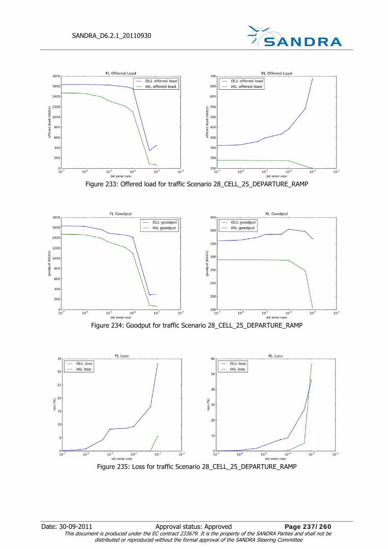
SANDRA_D6.2.1_20110930
Date: 30-09-2011 Approval status: Approved Page 237/260 This document is produced under the EC contract 233679. It is the property of the SANDRA Parties and shall not be
distributed or reproduced without the formal approval of the SANDRA Steering Committee
Figure 233: Offered load for traffic Scenario 28_CELL_25_DEPARTURE_RAMP
Figure 234: Goodput for traffic Scenario 28_CELL_25_DEPARTURE_RAMP
Figure 235: Loss for traffic Scenario 28_CELL_25_DEPARTURE_RAMP

SANDRA_D6.2.1_20110930
Date: 30-09-2011 Approval status: Approved Page 238/260 This document is produced under the EC contract 233679. It is the property of the SANDRA Parties and shall not be
distributed or reproduced without the formal approval of the SANDRA Steering Committee
Table 40 shows the latency for higher layer packets in FL direction for 4 different bit errors rates, broken down per COCR category. The priorities depend on the size as shown before and therefore packets from 10 000 to 100 000 bytes and packets larger than 100 000 bytes are listed separately. Table 41 shows the same information for the RL direction. This simple priority scheme seems to be enough to ensure that latency of the smaller packets is not affected significantly in the presence of the high bandwidth traffic.
Table 40: Average latency for high layer packets in Scenario 28, FL direction Secenario 28 average FL latency (ms) Priority 1.00e-07 BER 1.00e-06 BER 1.00e-05 BER 1.00e-04 BER DG-C 2.93 ± 0.00 2.93 ± 0.00 11.39 ± 15.23 59.47 ± 6.79 DG-D 5.72 ± 4.10 7.36 ± 2.41 38.55 ± 54.28 202.00 ± 62.38 DG-F 3.11 ± 0.00 4.11 ± 8.99 10.08 ± 8.90 71.93 ± 116.66 DG-J 4.90 ± 0.01 9.13 ± 6.97 47.57 ± 25.40 271.13 ± 69.60 DG-J (≥10k) 58.19 ± 25.35 99.56 ± 16.39 402.18 ± 24.73 973.19 ± 63.45 DG-K 10.85 ± 1.91 18.49 ± 1.08 97.04 ± 15.20 466.05 ± 0.12 DG-K (≥100k) 598595 ± 2857 614350 ± 2193 758054 ± 2985 887373 ± 18080 DG-K (≥10k) 58.37 ± 15.38 102.22 ± 5.05 392.56 ± 134.07 984.18 ± 171.48DG-L 8.36 ± 1.80 13.77 ± 8.77 71.17 ± 26.20 323.88 ± 36.97
Table 41: Average latency for high layer packets in Scenario 28, RL direction Scenario 28 average RL latency (ms) Priority 1.00e-07 BER 1.00e-06 BER 1.00e-05 BER 1.00e-04 BER DG-C 38.55 ± 1.45 38.95 ± 2.55 49.73 ± 11.58 141.35 ± 23.78 DG-D 42.09 ± 2.88 43.84 ± 13.81 67.01 ± 32.97 244.04 ± 8.44 DG-F 51.56 ± 4.18 58.70 ± 5.37 107.22 ± 12.06 503.50 ± 62.96 DG-J 39.46 ± 0.23 41.26 ± 0.45 58.60 ± 2.65 197.73 ± 5.71 DG-K 43.58 ± 0.45 48.11 ± 0.36 83.66 ± 23.31 327.79 ± 29.48 DG-K (≥100k) 27112 ± 409 32269 ± 1568 68431 ± 2082 126814 ± 2423 DG-K (≥10k) 96.09 ± 34.57 114.95 ± 31.08 311.55 ± 34.55 850.27 ± 155.26 DG-L 42.98 ± 0.95 44.52 ± 0.59 60.25 ± 24.06 182.32 ± 60.96 DG-L (≥10k) 180.87 ± 35.26 226.30 ± 83.38 523.55 ± 9.92 1256.64 ± 201.08
11.5 Summary and Conclusion
During the course of the SANDRA project a data traffic load analysis has been conducted which showed that applications with significant load requirements would justify the introduction of a broadband wireless communication system for airport surface communications. Furthermore, MAC performance simulations have shown performance figures to be expected by a future AeroMACS system. The implementation of the MAC layer in our simulation provided performance results for throughput and latency with standard settings. Additionally, we have investigated the various ARQ options defined by the IEEE 802.16 standard. The different aspects of the distinct ARQ options have been shown through simulation results. Furhtermore, a simulation scenario has used data traffic profiles as input. The results of the MAC simulation campaign showed reasonable values as long as the channel quality was acceptable, i.e. BER was less than 10-5.

SANDRA_D6.2.1_20110930
Date: 30-09-2011 Approval status: Approved Page 239/260 This document is produced under the EC contract 233679. It is the property of the SANDRA Parties and shall not be
distributed or reproduced without the formal approval of the SANDRA Steering Committee
12 AeroMACS Security Design The AeroMACS security is derived from the WiMAX security. In this chapter the WiMAX security is described and analyzed. For identified security issues some possible solutions are proposed. To obtain this target the following steps have been applied:
1. The WiMAX Forum security choices are indicated. They are detailed in the WiMAX ForumTM Mobile System Profile [WiF5] to define the security features implemented by the WiMAX terminals.
2. These features are analyzed considering the SESAR AeroMACS System Requirement Document [SES1] and the assessment of security provisions of the IEEE 802.16 standard released by the NASA [NAS09].
12.1 WiMAX Security Functions
12.1.1 Privacy and Key Management Protocol
WiMAX ForumTM (WMF) has decided to support Privacy Key Management (PKM) version 2 (PKMv2). This protocol, defined the first time in [WiM02] solves some shortcomings of the first version (PKMv1). Derivation of the authorization key, initially done only by BS, is now derived by the contribution of both parties using well known standards such as RSA and EAP. Additionally, BS is extended with a certificate, allowing for mutual authentication with the MS, which was missing in PKMv1. Finally, nonces, arbitrary numbers used only once to sign a cryptographic communication, are incorporated in order to avoid replay attacks.
12.1.2 Signalling and Data Protection
WiMAX Forum has decided to support CCM (Counter with Cipher Block Chaining Message Authentication Code) for Data Encryption which is considered the most secure cryptographic suite defined in the IEEE 802.16-2009 standard. In this way, the integrity and confidentiality of user data are guaranteed. One of major lacks of security in the IEEE 802.16-2009 standard, is related to the MAC management messages. The integrity of the MAC management messages is only supported after initial registration, and MAC messages are not protected from modification or involuntary changes. Moreover the MAC management messages are always sent on air in clear mode without any warranty of confidentiality. WMF did not solve these issues.
12.1.3 AAA Framework
AAA stands for Authentication, Authorization and Accounting. In the telecommunications networks these words are associated with the following functions:
• Authentication. It refers to the process where an entity (e.g. MS) is authenticated from the network by providing evidence that it holds a specific identity such as an identifier associated with credentials (e.g. password, digital certificates).
• Authorization. This function determines whether a particular entity is authorized to perform a given activity in a network, typically inherited from authentication when logging on to an application or service.
• Accounting. It refers to the tracking of network resource consumption by users making activities for the purpose of capacity and trend analysis, cost allocation, billing.
The Authentication function assumes that the entity to authenticate is provisioned with one or more credentials. There are two types of credentials. A device credential is used for authenticating the terminal device to the network. A user credential is used for authenticating the user of the access service to the network. A device credential could also be used as a user credential. That is possible when the user is

SANDRA_D6.2.1_20110930
Date: 30-09-2011 Approval status: Approved Page 240/260 This document is produced under the EC contract 233679. It is the property of the SANDRA Parties and shall not be
distributed or reproduced without the formal approval of the SANDRA Steering Committee
uniquely identified (e.g. using the MAC address of the device). In that special case, a single credential provisioned in the device can be used for authenticating both the device and the user at the same time. Credentials may come in different forms, such as username-password pair, SIM card, X.509 certificates, etc. The WiMAX AAA framework is based on IETF specifications (RFC 2865 and RFC 2866) and the WiMAX Forum standards support only the Extensible Authentication Protocol (EAP - RFC 3748) like authentication method although the IEEE 802.16-2009 supports also RSA methods. Figure 236 presents the WMF entities engaged in the AAA activities.
Figure 236: WiMAX AAA framework entities
Access Service Network (ASN) is defined as a complete set of network functions needed to provide radio access to a WiMAX user. ASN comprises network elements such as one or more Base Station(s), and one or more ASN Gateway(s). Connectivity Service Network (CSN) is defined as a set of network functions that provide IP connectivity services to the WiMAX user(s). Network Access Provider (NAP) is a business entity that provides WiMAX radio access infrastructure to one or more WiMAX Network Service Providers (NSPs). A NAP could implement this infrastructure using one ASN. Network Service Provider (NSP) is a business entity that provides IP connectivity and WiMAX services to WiMAX users compliant with the Service Level Agreement it establishes with WiMAX users. To provide these services, an NSP establishes contractual agreements with one or more NAPs. Additionally, an NSP MAY also establish roaming agreements with other NSPs and contractual agreements with third-party application providers (e.g., ASP or ISPs) for providing WiMAX services to users. From a WIMAX user standpoint, an NSP MAY be classified as Home NSP (H-NSP or H-CSN) or Visited NSP (V-NSP or V-CSN). The WiMAX AAA network access authentication procedure is used for authorizing the MS to receive the WiMAX access service. The procedure involves authentication of user and optionally device credentials. The functional blocks that are involved in the authentication procedure are presented below.

SANDRA_D6.2.1_20110930
Date: 30-09-2011 Approval status: Approved Page 241/260 This document is produced under the EC contract 233679. It is the property of the SANDRA Parties and shall not be
distributed or reproduced without the formal approval of the SANDRA Steering Committee
Table 42: Functional blocks involved in the authentication procedure Entity Function MS Acts as the EAP peer. NAS Consists of the EAP authenticator and is the receiver of service authorization attributes. It resides
in the ASN (ASN-GW). VAAA The AAA proxy that resides in the V-CSN. HAAA The AAA server that resides in the H-CSN. The EAP authentication server typically resides within
this AAA server. The AAA server has access to the user profiles and is also involved in the authentication of the mobility operations.
Other AAA proxies such as those in transit networks are not considered. It is assumed that transit proxies are trusted and act in a pass-through fashion and do not modify the RADIUS packets other than modifications made for routing purposes. After successful network access authentication, the HAAA delivers authorization attributes to the NAS.
Each EAP authentication involves executing an EAP method (e.g., EAP-TLS, EAP-TTLS, EAP-AKA). There are three EAP methods foreseen in the WiMAX AAA framework:
• EAP-TLS for device authentication based on X.509 certificates (RFC 5216)
• EAP-TTLS for user authentication (RFC5281)
• EAP-AKA for user authentication (RFC 4187)
12.1.3.1 EAP-TLS
In the WiMAX AAA framework whether or not to perform device authentication using EAP-TLS is up to the operator's policy. The EAP-TLS conversation will typically begin with the authenticator (NAS) and the peer (MS) negotiating EAP. The authenticator will then typically send an EAP-Request/Identity packet to the peer, and the peer will respond with an EAP-Response/Identity packet to the authenticator, containing the peer's user-Id. From this point forward, while nominally the EAP conversation occurs between the EAP authenticator and the peer, the authenticator could act as a pass-through device, with the EAP packets received from the peer being encapsulated for transmission to a backend authentication server (AAA server). During the successive phase of the EAP method the peer will send the own X.509 certificate to the server and the server could send the own X.509 certificate to the peer, if mutual authentication is enabled.
The core of this method is that there is certificate X.509 installed in the MS and is what gives EAP-TLS its authentication strength. A compromised password is not enough to break into EAP-TLS enabled systems because the intruder still needs to have the peer-side private key. The disadvantages to support X.509 certificate are that:
• It is necessary a Certification Authority to validate them
• The certificates expire and must be changed,
• The certificates must be purchased.
In particular the procedure to securely distribute, change and revoke the certificates can be cumbersome and prevent an easy deployment of the terminals.

SANDRA_D6.2.1_20110930
Date: 30-09-2011 Approval status: Approved Page 242/260 This document is produced under the EC contract 233679. It is the property of the SANDRA Parties and shall not be
distributed or reproduced without the formal approval of the SANDRA Steering Committee
12.1.3.2 EAP-TTLS
When it is used, the MS and AAA SHALL support TTLS version 0 and MS-CHAPv2 as a tunneled authentication protocol. When EAP-TTLS is used, the user credential shall be the identifier and password used for MSCHAPv2. EAP-TTLS is an EAP method that encapsulates a TLS session, consisting of a handshake phase and a data phase. During the handshake phase, the server is authenticated to the client (or client and server are mutually authenticated) using standard TLS procedures and keying material is generated in order to create a cryptographically secure tunnel for information exchange in the subsequent data phase. During the data phase, the client is authenticated to the server (or client and server are mutually authenticated) using an arbitrary authentication mechanism encapsulated within the secure tunnel (the WMF requires the MS-CHAPv2 mechanism). With this method the client is not required to be authenticated via a certificate to the server. This greatly simplifies the setup procedure as a certificate does not need to be installed on every client.
12.1.3.3 EAP-AKA
The EAP-AKA is a mechanism for authentication and session key distribution that uses the 3rd generation Authentication and Key Agreement mechanism, specified for Universal Mobile Telecommunications System (UMTS) and CDMA2000. AKA is based on challenge-response mechanisms and symmetric cryptography and it typically runs in a UMTS Subscriber Identity Module (USIM) or a CDMA2000 (Removable) User Identity Module ((R)UIM).
EAP-AKA works in the following manner:
• The identity module and the H-CSN have agreed on a secret key beforehand.
• The actual authentication process starts by having the HAAA produce an authentication vector, based on the secret key and a sequence number. The authentication vector contains a random part RAND, an authenticator part AUTN used for authenticating the network to the identity module, an expected result part XRES, a 128-bit session key for integrity check IK, and a 128-bit session key for encryption CK.
• The RAND and the AUTN are delivered to the identity module in the MS.
• The identity module verifies the AUTN, again based on the secret key and the sequence number. If this process is successful (the AUTN is valid and the sequence number used to generate AUTN is within the correct range), the identity module produces an authentication result RES and sends it to the home environment.
• The HAAA verifies the correct result from the identity module. If the result is correct, IK and CK can be used to protect further communications between the identity module and the HAAA.
EAP-AKA supports directly mutual authentication between HAAA and MS but requires that in each devices it is installed an USIM. The most important advantage of using USIM for authentication is that they may be used with different devices (e.g. MS) without losing the information stored on them.

SANDRA_D6.2.1_20110930
Date: 30-09-2011 Approval status: Approved Page 243/260 This document is produced under the EC contract 233679. It is the property of the SANDRA Parties and shall not be
distributed or reproduced without the formal approval of the SANDRA Steering Committee
12.2 AeroMACS Security Features
12.2.1 Privacy and Key Management Protocol
AeroMACS supports PKMv2 like WiMAX.
12.2.2 Signalling and Data Protection
The AeroMACS privacy and confidentiality requirements can be easily met with standard WiMAX encryption systems, and it is not expected to need stronger encryption techniques. Improving the encryption and association mechanisms would be possible, but it would mean to also modify some protocols and drivers compared to the legacy WiMAX devices. Although this is possible, the direct and indirect costs of this approach do not seems to be justified, especially considering the compliance, conformity and vulnerability testing to be performed on the new devices. The only important difference with respect to the WiMAX is on the minimum required compliance. PKMv2 should be considered mandatory and the use of PKMv1 should be prohibited. WiMAX standard security, however, is lacking in two main aspects, one at physical layer and one in the control (signaling) layer. About the physical layer, i.e., against jamming and other radio interference sources, it is not possible to derive further security measure beside the ones already covered by the airport area regulations. Usually local regulations cover this kind of problems, prohibiting or limiting the possible interference sources in the airport proximity. In case of voluntary jamming, e.g., whereas the Risk Assessment process can identify a possibility of voluntary jamming (basically in countries where there is a lack of regulations or similar), the only successful option is to limit the AeroMACS use to non-critical data transport and/or to use backup channels and technologies according to the kind of disturbance. This kind of attack (voluntary or involuntary) is usually mitigated by the WiMAX dynamic frequency selection mechanisms. Thus, in order to be effective, it should encompass a large number of frequencies. Due to this specificity and the need for very unusual transmission devices, the probability of such an attack is classified as unlikely. Nevertheless, whereas deemed necessary, airports and operators should adopt techniques to physically identify any jamming source. The control (signaling) channel represents the other major issue. As noted previously, the MAC management messages are not authenticated until the user is registered. Moreover they can be forged and, thus, are perfect to attack the user and create Denial of Services. The summary of MAC management messages is given in Table 43.
Table 43: MAC management messages, from IEEE Std 802.16-2009 Type Message name Message description Connection 0 UCD UL channel descriptor Fragmentable broadcast 1 DCD DL channel descriptor Fragmentable broadcast 2 DL-MAP DL access definition Broadcast 3 UL-MAP UL access definition Broadcast 4 RNG-REQ Ranging request Initial ranging or basic 5 RNG-RSP Ranging response Initial ranging or basic 6 REG-REQ Registration request Primary management 7 REG-RSP Registration response Primary management 8 — Reserved — 9 PKM-REQ Privacy key management request Primary management

SANDRA_D6.2.1_20110930
Date: 30-09-2011 Approval status: Approved Page 244/260 This document is produced under the EC contract 233679. It is the property of the SANDRA Parties and shall not be
distributed or reproduced without the formal approval of the SANDRA Steering Committee
10 PKM-RSP Privacy key management response Primary management or broadcast10
11 DSA-REQ Dynamic service addition request Primary management 12 DSA-RSP Dynamic service addition response Primary management 13 DSA-ACK Dynamic service addition acknowledge Primary management 14 DSC-REQ Dynamic service change request Primary management 15 DSC-RSP Dynamic service change response Primary management 16 DSC-ACK Dynamic service change acknowledge Primary management 17 DSD-REQ Dynamic service deletion request Primary management 18 DSD-RSP Dynamic service deletion response Primary management 19 - 20
— Reserved —
21 MCA-REQ Multicast assignment request Primary management 22 MCA-RSP Multicast assignment response Primary management 23 DBPC-REQ DL burst profile change request Basic 24 DBPC-RSP DL burst profile change response Basic 25 RES-CMD Reset command Basic 26 SBC-REQ SS basic capability request Basic 27 SBC-RSP SS basic capability response Basic 28 CLK-CMP SS network clock comparison Broadcast 29 DREG-CMD De/Reregister command Basic 30 DSX-RVD DSx received message Primary management 31 TFTP-CPLT Config file TFTP complete message Primary management 32 TFTP-RSP Config file TFTP complete response Primary management 33 ARQ-Feedback Stand-alone ARQ feedback Basic 34 ARQ-Discard ARQ discard message Basic 35 ARQ-Reset ARQ reset message Basic 36 REP-REQ Channel measurement report request Basic 37 REP-RSP Channel measurement report response Basic 38 FPC Fast power control Broadcast 39-43 Reserved — — 44 AAS-FBCK-REQ AAS feedback request Basic 45 AAS-FBCK-RSP AAS feedback response Basic 46 AAS_Beam_Select AAS beam select message Basic 47 AAS_BEAM_REQ AAS beam request message Basic 48 AAS_BEAM_RSP AAS beam response message Basic 49 DREG-REQ SS deregistration message Basic 50 MOB_SLP-REQ Sleep request message Basic 51 MOB_SLP-RSP Sleep response message Basic or broadcast 52 MOB_TRF-IND Traffic indication message Broadcast 53 MOB_NBR-ADV Neighbour advertisement message Broadcast, Primary
management
54 MOB_SCN-REQ Scanning interval allocation request Basic
10 For SSs and BSs that support PKMv2, PKM-RSP is sometimes transmitted on the broadcast connection.

SANDRA_D6.2.1_20110930
Date: 30-09-2011 Approval status: Approved Page 245/260 This document is produced under the EC contract 233679. It is the property of the SANDRA Parties and shall not be
distributed or reproduced without the formal approval of the SANDRA Steering Committee
55 MOB_SCN-RSP Scanning interval allocation response Basic 56 MOB_BSHO-REQ BS HO request message Basic 57 MOB_MSHO-REQ MS HO request message Basic 58 MOB_BSHO-RSP BS HO response message Basic 59 MOB_HO-IND HO indication message Basic 60 MOB_SCN-REP Scanning result report message Primary management 61 MOB_PAG-ADV BS broadcast paging message Broadcast 62 MBS_MAP Multicast and broadcast service MAP message —
63 PMC_REQ Power control mode change request message Basic
64 PMC_RSP Power control mode change response message Basic
65 PRC-LT-CTRL Setup/Tear-down of long-term MIMO precoding Basic
66 MOB_ASC-REP Association result report message Primary management 67 MOB_MIH-MSG MIH Payload Transfer message Primary management 68 SII-ADV Service Identity Information Advertisement
broadcast message Fragmentable broadcast
69 LBS-ADV Location information broadcast for LBS Broadcast
Basic connection: Connection that is established during MS initial ranging and used to transport delay-intolerant MAC layer management messages. The messages are not protected until the authentication procedure is completed. Broadcast connection: The management connection used by BS to send MAC layer management messages on DL to all MSs. The broadcast connection is identified by a well-known connection identifier (CID). A fragmentable broadcast connection is a connection that allows fragmentation of broadcast MAC management messages. These messages are not protected because the broadcast connection is always unciphered. Primary management connection: A connection that is established during initial subscriber station (SS) ranging and used to transport delay-tolerant MAC layer management messages. These messages are always protected because the Primary Connection is ciphered. Adding a cryptographic mechanism to protect them seems to be unfeasible, as it would require changes in the devices that would make it hard to adopt legacy WiMAX elements in AeroMACS devices. The only feasible approach is to consider the presence of spurious MAC management packets as a symptom of the presence of a rogue terminal attempting to attack the system. The response to such an event might range from switching off the AeroMACS system, to limiting the transmission to some kind of data (e.g., high priority), to active multilateration of the rogue device. AeroMACS can cope with the spurious messages with internal mechanisms, or by programming special reactions to unexpected messages (e.g., fast BS switching, network re-join, etc., see also [NAS09]), however the increased network overhead, battery use and ultimately the increased network latency for the associated and attacked devices, should lead to the conclusion that those kind of attacks can not be underestimated. Moreover the “internal” mitigation mechanisms can hide a network attack, thus it is imperative to log any unexpected MAC control message and to gather periodically those information.

SANDRA_D6.2.1_20110930
Date: 30-09-2011 Approval status: Approved Page 246/260 This document is produced under the EC contract 233679. It is the property of the SANDRA Parties and shall not be
distributed or reproduced without the formal approval of the SANDRA Steering Committee
12.2.3 AAA Framework
The AeroMACS AAA framework will be based on the WiMAX AAA one. The open points remained to be solved in order to drive the standardization of the AeroMACS AAA framework are the authentication method to be used and the presence of multiple domains that could deliver services to the AeroMACS MS.
12.2.3.1 Authentication Methods
In [SES1], it is indicated that AeroMACS supports the WiMAX AAA framework with the following notes:
• It is proposed to stick to the WiMAX forum profiles and thus we do not consider device authentication. Nevertheless the need for user and device authentication will be investigated in SESAR as well as the methodology to implement device authentication.
• RSA is not currently supported by the WiMAX Forum, only EAP is supported. However RSA is more
robust and could be preferred to EAP depending on the results of the Security analysis, which will be conducted in the frame of SESAR.
The first bullet highlights the main issue for the definition of the AeroMACS AAA framework. In the WiMAX networks, much like in the 3GPP ones, it is possible to buy a MS from the operator or from a store and to use it with the credentials agreed with the operator. For this reason solutions like EAP-TTLS in which the subscriber need only to use the own credentials to access to the networks irrespective of the terminal (e.g. the mobile phone market) are preferable. EAP-AKA is as well a perfectly valid system, as from an operational point of view the user will acquire from the operator an USIM, effectively providing user’s authentication to the operator. The EAP-AKA seems as well more robust as the User will not risk to loose or forget the authentication data, and the operator can bind any number of USIMs to a single user. For AeroMACS AAA framework the main advantages to use EAP-AKA are:
• It is possible to change the USIM/(R)UIM without changing the software of the MS.
• It is possible to change the security algorithm without changing the software of the MS but only changing the USIM/(R)UIM. • A MS without USIM/(R)UIM is not able to enter in the AeroMACS network.
• It is possible to develop the MS in a way that if it is stolen or if someone tries to extract the USIM/(R)UIM, MS and USIM/(R)UIM will become unusable (anti tampering protection).
To increase the level of security it is possible to use EAP-AKA’ in the place of EAP-AKA. EAP-AKA’ is an extension to EAP-AKA mechanism that aims at limiting the effects of a compromised access network nodes and devices. The goal is met by defining a new key derivation function that binds the keys derived to the name of the access network. EAP-AKA’ is particularly interesting for WiFi or WiMAX systems, where user’s mobility cannot ensure the use of a trusted access infrastructure. The use of EAP-AKA’ over EAP-AKA in AeroMACS is mainly dependent on threats evaluation. Using EAP-AKA’ could be unnecessary if the assumption that AeroMACS infrastructures are controlled and trusted holds.
12.2.3.2 Multiple Domains
An AeroMACS MS could receive services from different Application Domains and it is necessary that the MS is authenticated from each of them. The MS is authenticated by its Home CSN using the standard WiMAX Forum procedure and in this way it is able to use services supplied directly by the Home CSN. The WMF

SANDRA_D6.2.1_20110930
Date: 30-09-2011 Approval status: Approved Page 247/260 This document is produced under the EC contract 233679. It is the property of the SANDRA Parties and shall not be
distributed or reproduced without the formal approval of the SANDRA Steering Committee
Forum procedures do not consider additional authentication procedures for services supplied from other Application Domains. In this paragraph is described a possible solution to solve this issue. Figure 237 describes a possible AeroMACS initial MS network procedure comprising MS-to-Network EAP authentication process and multiple Domain authentications.
MS
(1) DL channel acquisition, MAC synchronisation (DL-MAP) and obtaining
UL channel parameters
(2) Initial Ranging and PHY adjustments process (RNG-REQ/ RSP)
(8) EAP Authentication Method(e.g. EAP-TTLS, EAP-TLS, EAP-AKA)
(9) EAP Success is indicated and security
context is acquired
(5) PKMv2-RSP/EAP Transfer (EAP Request/ Identity)
(6) PKMv2-REQ/EAP-Transfer(EAP Response/ Identity -NAI)
(11) PKMv2-RSP/EAP-Transfer(EAP Success)
(14) PKMv2-RSP/SA-TEK-Challenge
(15) PKMv2-REQ/SA-TEK-Request
(16) PKMv2-RSP/SA-TEK-Response
(17) PKMv2-REQ/Key-Request
(18) PKMv2-RSP/Key-Reply
(4) AuthRelay_EAP_Transfer(EAP Payload: EAP Request/Identity)
(7) AuthRelay_EAP_Transfer(EAP Response / Identity-NAI)
(12) Key_Change_Directive(AK Context)
(13) Key_Change_Ack
(10) AuthRelay_EAP_Transfer(EAP Payload, EAP-Success)
(21) IP Address Allocation
Authenticator / ASN-GW
Visited - AAA Server
Home -AAA Server
DHPCServer
Domain X AAABS
(22) Domain X Authentication procedure
(23) Domain Y Authentication procedure
Domain Y AAA
(3) MS Pre Attachment Procedure (SBC-REQ/RSP, MS_PreAttachment_Req/RSP/ACK)
(19) MS Registration Procedure
(20) Data Path Establishment
Figure 237: A possible AeroMACS initial MS network procedure

SANDRA_D6.2.1_20110930
Date: 30-09-2011 Approval status: Approved Page 248/260 This document is produced under the EC contract 233679. It is the property of the SANDRA Parties and shall not be
distributed or reproduced without the formal approval of the SANDRA Steering Committee
AeroMACS MS Network Entry starts:
STEP1: DL channel acquisition, MAC synchronization and obtaining UL channel parameters.
STEP2: Initial Ranging round trips, RNG-REQ/ RNG-RSP message exchange.
STEP3: Pre-Attachment procedure. MS starts Basic Capabilities negotiation where MS and BS among other
parameters negotiate the PKM protocol version and Authorization Policy.
STEP4: The Authenticator (in ASN/ASN GW) initiates EAP authentication procedure with MS. The trigger
for it, it’s the successful end of the MS Pre-Attachment procedure.
STEP5: The BS relays the EAP Request/ Identity to the MS.
STEP6: MS responds with EAP Response/ Identity message providing Identity.
STEP7: BS relays EAP payload received to the Authenticator over Authentication Relay protocol.
STEP8: The Authenticator analyses the Identity provided by the MS. Depending on the domain the MS
could be locally authenticated (the MS is in its Home Network) or not (the MS is in a Visited Network). If
the MS is in a Visited Network EAP payload are forwarded to the MS’ Home AAA server via the Visited AAA
server. In order to deliver the EAP payload to the AAA server, the Authenticator forwards the EAP message
via a collocated AAA client using RADIUS Access-Request message.
The EAP authentication process (tunneling EAP authentication method) is performed between the MS and
the Authentication server via the Authenticator in ASN/ASN-GW. BS provides “relay” of EAP payload from
PKMv2 EAP-Transfer messages to AR_EAP_Transfer and vice versa. The Authenticator in ASN/ASN-GW acts
in pass through mode and forwards the EAP messages received as a payload from the BS in
AR_EAP_Transfer messages to the AAA server using RADIUS Access-Request messages and vice versa.
There can be multiple EAP message exchanges between the MS and AAA server.
EAP peers (supplicant in MS and authentication server) negotiate the EAP method (e.g. EAP-AKA, EAP-
TTLS, EAP-TLS) and perform it.
STEP9: The Authenticator receives indication about the successful completion of EAP-based authentication,
the MS authorization profile and the required security context.
STEP10: The Authenticator forwards EAP results (EAP-Success or EAP-Failure message) to BS.
STEP11: The BS relays EAP payload to the MS in PKMv2 EAP-Transfer/ PKM-RSP message. This message
indicates the results of EAP authentication round to the Supplicant in the MS. The BS continues waiting for
the explicit indication of EAP authentication completion from the Authenticator.
STEP12: The Authenticator in ASN/ASN-GW sends Key_Change_Directive message to the BS to indicate
completion of the EAP authentication process.
STEP13: BS receiving Key_Change_Directive from Authenticator will acknowledge it by Key_Change_Ack
message.
STEPS 14, 15, 16: PKMv2 3-way handshake (SA-TEK-Challenge/Request/Response exchange) is
conducted between BS and MS to verify the AK to be used and to establish the Security Association(s) pre-
provisioned for the MS
STEPS 17, 18: MS acquires the valid TEK keys using PKMv2 Key-Request/ Reply exchange between MS
and BS for each SA

SANDRA_D6.2.1_20110930
Date: 30-09-2011 Approval status: Approved Page 249/260 This document is produced under the EC contract 233679. It is the property of the SANDRA Parties and shall not be
distributed or reproduced without the formal approval of the SANDRA Steering Committee
STEP19: When PKMv2 3-way handshake is completed, MS proceeds with 802.16e Registration procedure
by sending REG-REQ message. This message will carry the MS supported capabilities (such as CS
capabilities, Mobility parameters and Handover support, etc.).
STEP20: The ASN-GW starts to configure the BS and the MS using the MS QoS profile received by the
Home AAA at step 9. The BS verifies whether there are sufficient radio resources and it decides whether
the request should be accepted or not. In case of acceptance, the configuration is sent to the MS. MS
accepts or rejects the configuration according to the standard. At this step all the Service Flows are
configured and ready, irrespective of the application domains associated with them.
STEP21: IP address allocation procedure. When the MS will have a valid IP address all Services Flows
associated with services directly provided by the Home CSN could be immediately used.
STEP22: Application-level Services authentication procedure between MS and Domain X AAA11. When this
procedure is properly terminated all Service Flows associate with services provided by Domain X CSN could
be used.
STEP23: Application-level Services authentication procedure between MS and Domain Y AAA12. When this
procedure is properly terminated all Service Flows associate with services provided by Domain Y CSN could
be used.
About the last two steps, we shall remark that application-level services (e.g., VoIP, APC flows, etc.) can
require an AAA procedure. Those are functionally and logically disjoint from the AeroMACS AAA. Any
service is free, with this regard, to “trust” the lower level authentication or to require a new authentication
in order to be used, eventually with a CSN different then the one authenticating the AeroMACS device. This
approach is fully compliant with the current Internet approach, where the authentication to the access
network does not necessarily imply the authentication to the services provided by other application-level
service providers.
In brief the main advantages of this solution are:
• For each MSs, the service flows configuration is centralized in the Home AAA.
• Each application domain, different from the home, can choose the own authentication method
transparently regarding other domains.
11 This procedure is out of scope for AeroMACS 12 This procedure is out of scope for AeroMACS

SANDRA_D6.2.1_20110930
Date: 30-09-2011 Approval status: Approved Page 250/260 This document is produced under the EC contract 233679. It is the property of the SANDRA Parties and shall not be
distributed or reproduced without the formal approval of the SANDRA Steering Committee
APPENDIX A
Following tables summarize BER results for 5 and 10 MHz profiles in LOS and NLOS conditions and with
different modulation schemes.
Simulation Results with 5 MHz Bandwidth
5 MHz, QPSK, CP=1/8Ts, LOS
FL RL
BER BER
Eb/N0[dB] 1slot/LIN Eb/N0[dB] 1slot/LIN
0 3,654E-01 0 4,206E-01
3 1,836E-01 3 2,873E-01
6 4,852E-02 6 7,493E-02
9 9,352E-03 9 9,838E-03
12 1,231E-03 12 8,869E-04
15 1,567E-04 15 2,971E-04
18 8,281E-05
Eb/N0[dB] 1slot/ID Eb/N0[dB] 1slot/ID
0 3,074E-01 0 3,849E-01
3 1,088E-01 3 2,020E-01
6 2,479E-02 6 4,539E-02
9 3,645E-03 9 5,462E-03
12 4,748E-04 12 4,735E-04
15 5,390E-05 15 3,905E-05
Eb/N0[dB] 195slot/LIN Eb/N0[dB] 102 slot/LIN
0 4,533E-01 0 4,784E-01
3 2,104E-01 3 3,344E-01
6 2,903E-02 6 9,104E-02
9 2,323E-03 9 9,178E-03
12 1,447E-04 12 6,349E-04
15 1,209E-07 15 3,659E-05
2,658E-06
Eb/N0[dB]
0
3
6
9
12
15
18
21
24

SANDRA_D6.2.1_20110930
Date: 30-09-2011 Approval status: Approved Page 251/260 This document is produced under the EC contract 233679. It is the property of the SANDRA Parties and shall not be
distributed or reproduced without the formal approval of the SANDRA Steering Committee
5 MHz, QPSK, CP=1/16Ts, LOS Eb/N0[dB] 1slot/LIN Eb/N0[dB] 1 slot/ID 0 3,608E-01 0 4,142E-01
3 1,749E-01 3 2,521E-01
6 4,174E-02 6 6,875E-02
9 6,790E-03 9 8,810E-03
12 1,140E-03 12 7,943E-04
15 1,357E-04 15 6,757E-05
5 MHz, QPSK, CP=1/8Ts, NLOS FL RL BER BER
Eb/N0[dB] 1slot/LIN Eb/N0[dB] 1slot/LIN
0 3,876E-01 0 4,257E-01
5 1,663E-01 3 3,132E-01
10 3,409E-02 6 1,595E-01
15 4,338E-03 9 4,920E-02
20 6,206E-04 12 1,110E-02
25 7,107E-05 15 1,693E-03
30 9,000E-06 18 2,198E-04
Eb/N0[dB] 1slot/ID
0 3,200E-01
5 1,120E-01
10 1,954E-02
15 2,736E-03
20 1,948E-04
Eb/N0[dB] 195 slot/LIN Eb/N0[dB] 102slot/LIN
0 4,511E-01 0 4,805E-01
5 1,607E-01 3 3,801E-01
10 1,246E-02 6 1,829E-01
12,5 1,845E-03 9 5,019E-02
15 2,767E-04 12 8,144E-03
17,5 3,328E-05 15 9,051E-04
20 2,362E-06 18 6,768E-05
21
Eb/N0[dB] 45 slot/LIN Eb/N0[dB] 45slot/LIN
0 1,731E-01 0 4,784E-01
5 1,419E-02 3 3,843E-01
15 3,353E-04 6 1,841E-01
9 4,970E-02
Eb/N0[dB] 102slot/LIN 12 7,923E-03
0 4,536E-01 15 9,448E-04
5 1,713E-01 18 7,496E-05
10 1,307E-02 21 7,289E-06
15 4,273E-04
20 4,151E-06
Eb/N0[dB] 60slot/LIN
0 4,573E-01
5 1,746E-01

SANDRA_D6.2.1_20110930
Date: 30-09-2011 Approval status: Approved Page 252/260 This document is produced under the EC contract 233679. It is the property of the SANDRA Parties and shall not be
distributed or reproduced without the formal approval of the SANDRA Steering Committee
10 1,611E-02
15 3,586E-04
Eb/N0[dB] 10slot/LIN
0 4,513E-01
5 1,772E-01
10 1,630E-02
12,5 3,361E-03 5 MHz, QPSK, CP=1/16Ts, NLOS Eb/N0[dB] 1slot/LIN Eb/N0[dB] 1slot/LIN
0 3,793E-01 0 4,227E-01
5 1,589E-01 3 3,040E-01
10 3,297E-02 6 1,437E-01
15 4,857E-03 9 4,737E-02
20 5,479E-04 12 9,710E-03
25 6,821E-05 15 1,524E-03
18 1,756E-04 5 MHz , 64-QAM, CP=1/8Ts, LOS FL RL BER BEREb/N0[dB] 1slot/LIN Eb/N0[dB] 1slot/LIN 0 4,912E-01 0 4,974E-01 3 4,740E-01 3 4,800E-01 6 4,242E-01 6 4,424E-01 9 2,761E-01 9 3,004E-01 12 1,751E-01 12 1,077E-01 15 9,582E-02 15 2,385E-02 18 7,452E-02 18 3,180E-03 21 3,494E-02 21 3,030E-04 24 3,157E-02 24 27 4,002E-06 Eb/N0[dB] 1slot/ID Eb/N0[dB] 1slot/ID 0 4,863E-01 0 3 4,390E-01 3 4,772E-01 6 3,659E-01 6 4,294E-01 9 1,391E-01 9 2,823E-01 12 4,769E-02 12 9,789E-02 15 7,435E-03 15 1,620E-02 18 9,732E-04 18 1,762E-03 21 1,189E-04 21 1,800E-04 24 24 1,681E-05 Eb/N0[dB] 195slot/LIN Eb/N0 102slot/LIN 0 4,980E-01 5 4,776E-01 3 4,602E-01 10 2,702E-01 6 2,114E-01 15 2,417E-02 9 2,036E-02 20 4,539E-04 12 2,920E-03 15 1,533E-03 18 1,372E-03 Eb/N0[dB] 195slot/ID 0 4,966E-01 5 4,338E-01 10 1,259E-01 15 3,480E-03 20 6,465E-06

SANDRA_D6.2.1_20110930
Date: 30-09-2011 Approval status: Approved Page 253/260 This document is produced under the EC contract 233679. It is the property of the SANDRA Parties and shall not be
distributed or reproduced without the formal approval of the SANDRA Steering Committee
5 MHz , 16-QAM, CP=1/8Ts, LOS Eb/N0 1slot/LIN Eb/N0 1slot/LIN
0 4,397E-01 0 4,677E-01
5 1,843E-01 5 2,729E-01
10 2,140E-02 10 2,130E-02
15 2,219E-03 15 4,822E-04
20 4,332E-04 20 8,079E-06
25 1,905E-04
Eb/N0 1slot/ID Eb/N0 1slot/ID
0 4,125E-01 0 4,614E-01
5 1,268E-01 5 2,280E-01
10 1,086E-02 10 1,395E-02
15 4,758E-04 15 3,128E-04
20 1,537E-05 20 4,079E-06
Eb/N0 195slot/LIN Eb/N0 102slot/LIN
0 4,785E-01 0 4,939E-01
5 1,936E-01 5 3,128E-01
10 1,198E-02 10 2,067E-02
12,5 1,842E-03 15 2,696E-04
15 3,020E-04 20 2,488E-06
17,5 4,425E-05
Eb/N0 45slot/LIN
0 4,799E-01
5 2,088E-01
10 1,443E-02
12,5 2,675E-03
15 4,613E-04
Simulation Results with 10 MHz Bandwidth
10 MHz, QPSK, CP=1/8Ts, LOS
FL RL
BER BER
Eb/N0[dB] 1slot/LIN Eb/N0[dB] 1slot/LIN
0 3,740E-01 0 4,120E-01
3 1,809E-01 3 2,551E-01
6 4,425E-02 6 8,511E-02
9 7,838E-03 9 1,485E-02
12 1,123E-03 12
15 1,544E-04 15
18 2,575E-05 18
Eb/N0[dB] 1 slot/ID

SANDRA_D6.2.1_20110930
Date: 30-09-2011 Approval status: Approved Page 254/260 This document is produced under the EC contract 233679. It is the property of the SANDRA Parties and shall not be
distributed or reproduced without the formal approval of the SANDRA Steering Committee
0 2,881E-01
3 1,107E-01
6 2,307E-02
9 3,360E-03
Eb/N0[dB] 390 slot/LIN Eb/N0[dB] 210 slot/LIN
0 4,479E-01 0 4,819E-01
2,5 2,635E-01 3 3,386E-01
5 6,052E-02 6 9,039E-02
7,5 7,794E-03 9 9,345E-03
10 8,270E-04
12,5 7,206E-05
10 MHz, QPSK, CP=1/16Ts, LOS Eb/N0[dB] 1slot/LIN Eb/N0[dB] 1slot/LIN
0 3,505E-01 0 2,514E-01
3 1,704E-01 3 7,600E-02
6 4,440E-02 6 1,230E-02
9 7,510E-03 9 1,655E-03
12 9,731E-04 12 1,710E-04
15 15 10MHz, QPSK, CP=1/8Ts, NLOS
FL RL
BER BER
Eb/N0[dB] 1slot/LIN Eb/N0[dB] 1slot/LIN
0 3,854E-01 0 4,187E-01
5 1,703E-01 3 3,118E-01
10 3,786E-02 6 1,516E-01
15 5,659E-03 9 4,793E-02
20 5,633E-04 12 7,924E-03
15 1,393E-03
Eb/N0[dB] 1 slot/ID Eb/N0[dB] 1slot/ID
0 3,104E-01 0
5 1,144E-01 3 2,585E-01
10 2,041E-02 6 1,069E-01
15 2,933E-03 9 2,920E-02
20 2,380E-04 12 4,881E-03
15 6,921E-04
Eb/N0[dB] 390 slot/LIN Eb/N0[dB] 210 slot/LIN
0 4,606E-01 0 4,865E-01
5 1,528E-01 3 3,936E-01
10 5,669E-03 6 1,759E-01
15 3,915E-05 9 3,333E-02
20 1,205E-06 12 3,254E-03
15 3,971E-05
Eb/N0[dB] 195 slot/LIN
0 4,723E-01

SANDRA_D6.2.1_20110930
Date: 30-09-2011 Approval status: Approved Page 255/260 This document is produced under the EC contract 233679. It is the property of the SANDRA Parties and shall not be
distributed or reproduced without the formal approval of the SANDRA Steering Committee
5 1,574E-01
10 6,144E-03
15 3,965E-05 10MHz, QPSK, CP=1/16Ts, NLOS Eb/N0[dB] 1slot/LIN Eb/N0[dB] 1 slot/ID
0 3,751E-01
5 1,572E-01 3 2,990E-01
10 3,669E-02 6 1,401E-01
15 5,731E-03 9 4,160E-02
20 5,877E-04 12 6,936E-03
25 5,476E-05 15 1,168E-03

SANDRA_D6.2.1_20110930
Date: 30-09-2011 Approval status: Approved Page 256/260 This document is produced under the EC contract 233679. It is the property of the SANDRA Parties and shall not be
distributed or reproduced without the formal approval of the SANDRA Steering Committee
APPENDIX B
Appendix B1 In this Appendix we highlight the major steps leading to the false alarm probability in the detection of the frame preamble. For this purpose, we write the received samples as r(k) = rR (k)+ jrI (k) and assume
that rR (k) and rI (k) are statistically independent and Gaussian distributed with zero mean and variance
σ r2 . By invoking the Central Limit Theorem (CLT), we can reasonably model the real and imaginary parts
of the correlation C(d) defined in (Eq.17) as statistically independent Gaussian random variables with zero
mean and variance σ c2 = σ r
4 / Nc . Accordingly, the magnitude of C(d) is a chi-square random variable with two degrees of freedom and a distribution function
{ } 2 2F( ) Pr ( ) 1 exp[ /(2 )]cz C d z z σ= ≤ = − − . (Eq.B1.1)
To simplify the analysis, we replace the denominator in (Eq.B1.1) with the expectation E{P(d)} which, in the absence of any frame preamble, takes the form E{P(d)} = 2σ r
2 . (Eq.B1.2)
The false alarm probability is thus given by
{ }20 0Pr{ ( ) } Pr ( ) 2fa rP M d C dλ λ σ= > = > (Eq.B1.3)
or, bearing in mind (Eq.B1.1),
Pfa = 1− F(2λ0σ r2 ) = exp(−2λ0
2Nc ) . (Eq.B1.4)
Appendix B2
In this Appendix we compute the variance of the frequency estimate ε given in (Eq.44). For this purpose, we use (Eq.41) and (Eq.43), which hold true provided that IBI is negligible. Letting η = ηR + jηI and
assuming that η is much less than unity, from (Eq.41) and (Eq.43) it follows that
ε = ε +1
2πηI . (Eq.B2.1)
On the other hand, inspection of (Eq.43) indicates that η is zero-mean. Hence, taking the expectation in
both sides of (Eq.B2.1), it turns out that ε is unbiased with variance
{ }22
1ˆvar{ } E4 Iε ηπ
= (Eq.B2.2)
or, equivalently,
{ }2 22
1ˆvar{ } E e[ ]8
ε η ηπ
= −ℜ (Eq.B2.3)
where we have used the identity ηI = (η −η∗) / (2 j) . To proceed further, we use (Eq.43) and observe
that the noise terms %w(dk ,m ) and
%w(dk ,m + N ) are statistically independent for different values of k and
m with zero-mean and variance σw2 . Hence, after standard calculations it is found that { }2E 0η = and
{ }2 1 22 1E SNR SNRB g B gM N M N
η − −= + . (Eq.B2.4)

SANDRA_D6.2.1_20110930
Date: 30-09-2011 Approval status: Approved Page 257/260 This document is produced under the EC contract 233679. It is the property of the SANDRA Parties and shall not be
distributed or reproduced without the formal approval of the SANDRA Steering Committee
Finally, substituting these results into (Eq.B2.3) leads to (Eq.45).
Appendix B3 In this Appendix we derive the ML estimates of the quantities dl and
[ (0), (1), , (35)]l l l lKH = H H H starting from the DFT outputs X(im,v ) corresponding to the ranging
subcarriers. Using the model of X(im,v ) specified in (Eq.68), the log-likelihood function for the joint
estimation of the unknown parameters is found to be
,
235 32 /
, ,0 0
( , ) ( ) ( ) ( ) m vj d i Nm v m v
m vd X i c i m e π−
= =
Λ = − −∑∑ l%
l l l l% %% H H (Eq.B3.1)
where ( , )dl l%% H denotes a trial value of ( , )dl lH and we have skipped irrelevant terms and
multiplicative factors independent of ( , )dl l%% H . The ML estimates of the unknown parameters are found
as the location where ( , )dΛ l l%% H achieves its global maximum. We begin by keeping
%dl fixed and
maximize with respect to l%H . This yields
,3
2 /,
0
1ˆ ( ; ) ( )4
m vj d i Nm v
vm d Y i e π
=
= ∑ l%
l l l%H (Eq.B3.2)
with ,( )m vY il being defined in (Eq.65). Next, substituting (Eq.B3.2) into (Eq.B3.1) leads to the concentrated
likelihood function for dl in the form
35 35 32 2
,0 0 0
ˆ( ) 4 ( ; ) ( )c m vm m v
d m d X i= = =
Λ = −∑ ∑∑l l l% %H . (Eq.B3.3)
The ML estimate of dl is found by looking for the maximum of ( )c dΛ l% with
%dl varying in the set
max{0,1, , }dK . Then, collecting (Eq.B3.2) and (Eq.B3.3)it follows that maximizing ( )c dΛ l% is equivalent to
maximizing the objective function
,
235 32 /
,0 0
( ) ( ) m vj d i Nm v
m vd Y i e π
= =
′Λ = ∑ ∑ l%
l l% (Eq.B3.4)
as indicated in (Eq.70). The ML estimate of ( )mlH is eventually computed from (Eq.B3.2) by replacing
dl% with the timing estimate ( )ˆ MLdl .
Appendix B4 In this Appendix we highlight the major steps leading to the joint ML estimation of the quantities ε l and
[ (0), (1), , (35)]l l l lKH = H H H starting from the received time-domain samples
[ (0), (1), , ( 1)]r r r N= −r K . After skipping some irrelevant factors and additive terms, from (Eq.79) the log-likelihood function for the unknown parameters is found to be
,
21 35 32 ( ) /2 /
,0 0 0
1( , ) ( ) ( ) ( ) m vN
j i k d Nj k Nm v
k m vr k e c i m e
Nππ εε
−−
= = =
Λ = − −∑ ∑∑ ll%%
l l l l% %% H H (Eq.B4.1)

SANDRA_D6.2.1_20110930
Date: 30-09-2011 Approval status: Approved Page 258/260 This document is produced under the EC contract 233679. It is the property of the SANDRA Parties and shall not be
distributed or reproduced without the formal approval of the SANDRA Steering Committee
with ( , )ε l l%% H denoting a trial value of ( , )ε l lH . In order to locate the global maximum of ( , )εΛ l l
%% H ,
we begin by keeping %ε l fixed and maximize with respect to l%H . This yields
ˆ ( ; ) ( ; )m mε ε= Ωl l l% %H (Eq.B4.2)
where ( ; )m εΩ l% is defined in (Eq.81). Next, substituting (Eq.B4.2) into (Eq.B4.1) and performing standard
computations, we obtain the concentrated likelihood function for ε l in the form
35 1
2 2
0 0
( ) 4 ( ; ) ( )N
cm k
m r kε ε−
= =
Λ = Ω −∑ ∑l l% % . (Eq.B4.3)
The CFO estimate is found by looking for the maximum of ( )c εΛ l% with respect to ε l
% . From (Eq.B4.2) and
(Eq.B4.3) it follows that maximizing ( )c εΛ l% is equivalent to maximizing the objective function
35
2
0( ) ( ; )
mmε ε
=
′Λ = Ω∑l l% % (Eq.B4.4)
over the interval maxε ε≤l% as indicated in (Eq.81). Finally, the ML estimate of ( )mlH is obtained from
(Eq.B4.2) after replacing ε l% with ε l .
Appendix B5 In this Appendix we evaluate the false alarm probability of the binary test (Eq.78) for the detection of the ranging code cl . For this purpose, we rewrite (Eq.77) as
1 2( )
01 1 2
,0 0
1 ˆ ( )
1 ( )
MAH
mM V
m vm v
mM
X iMV
−
=− −
= =
Γ =∑
∑∑
l
l
H (Eq.B5.1)
where M = 36 is the number of tile in the ranging subchannel and V = 4 the number of subcarriers per
tile. The DFT output X(im,v ) is expressed in (Eq.61), while the estimate (AH)ˆ ( )mlH is obtained from
(Eq.71) after replacing ( )ˆ MLdl with ( )ˆ AHdl , yielding
( )
,1 ˆ2 /(AH)
, ,0
1ˆ ( ) ( ) ( )AH
m vV
j d i Nm v m v
v
m c i X i eV
π−
=
= ∑ l
l lH . (Eq.B5.2)
To proceed further, assume that cl is not present in the received ranging signal. Then, by invoking the
central limit theorem, we can reasonably model the quantities (AH)ˆ ( )mlH in (Eq.B5.2) as circularly
symmetric and statistically independent Gaussian random variables for 0,1, , 1m M= −K , each having zero-mean and variance
{ }22ˆ ,
1 E ( )m vX iV
σ =H
(Eq.B5.3)
with
{ }2 2,
1
E ( )K
m v w kk
X i Pσ=
= +∑ . (Eq.B5.4)

SANDRA_D6.2.1_20110930
Date: 30-09-2011 Approval status: Approved Page 259/260 This document is produced under the EC contract 233679. It is the property of the SANDRA Parties and shall not be
distributed or reproduced without the formal approval of the SANDRA Steering Committee
It follows that the numerator of Γl in (Eq.B5.1), say zl , is a chi-square random variable with 2M
degrees of freedom and pdf
p(z) =
MVσ
H2 (M −1)!
MVσ
H2 z
⎛
⎝⎜
⎞
⎠⎟
M −1
exp −MVσ
H2 z
⎛
⎝⎜
⎞
⎠⎟ z ≥ 0 . (Eq.B5.5)
To simplify the analysis, we replace the sample mean in the denominator of Γl by the expectation of
X(im,v )2, which is equal to
Vσ
H2 according to (Eq.B5.3). The false alarm probability is thus given by
{ }2ˆPr{ } PrfaP z Vλ λ σ= Γ > >l l H
(Eq.B5.6)
or, using (Eq.B1.1),
Pfa =MV
σH2 (M −1)!
MVσ
H2 z
⎛
⎝⎜
⎞
⎠⎟
M −1
exp −MVσ
H2 z
⎛
⎝⎜
⎞
⎠⎟
λVσH2
+∞
∫ dz . (Eq.B5.7)
Replacing the integration variable z by y = Mz /σ
H2 yields
Pfa =1
(M −1)!yM −1 exp −y( )
MVλ
+∞
∫ dy (Eq.B5.8)
which eventually leads to the result reported in (Eq.84).

SANDRA_D6.2.1_20110930
Date: 30-09-2011 Approval status: Approved Page 260/260 This document is produced under the EC contract 233679. It is the property of the SANDRA Parties and shall not be
distributed or reproduced without the formal approval of the SANDRA Steering Committee
APPENDIX C The channel estimation algorithms used for the Alamouti STC 2x1 implementation proposed in the standard (right figure) and for the alternative implementation STC-2 (left figure) are schematically illustrated in Figure 238. In both cases, the pilot interpolation in frequency domain is performed applying a first pilot interpolation in time direction and then a frequency interpolation. The frequency interpolation is made exploiting the values obtained in the first interpolation, according to the schemes of Figure 238.
Figure 238: Channel estimation scheme for the FL STC 2x1 case. WiMAX standard implementation (left) and STC-2 implementation
The alternative Alamouti STC 2x1 implementation [PUL_10aug] (STC-2) preserves the original frame structure of the system limiting the modifications required to the system. Figure 239 describes the implementation schemes.
Data sub-carrierPilot sub-carrier 1st antenna
xi,j
Pilot sub-carrier 2nd antenna
xi,j+1 xi,j+2 xi,j+3
xi+1,j
xi+2,j
xi+3,j
xi,j+..
...
xi,j xi,j+1 xi,j+2 xi,j+3
P1 xi+1,j+1 xi+1,j+2 xi+1,j+3
xi+2,j* xi+2,j+1
* xi+2,j+2* xi+2,j+3
*
P2 xi+3,j+1* xi+3,j+2
* xi+3,j+3*
P1
xi+1,j+..
P2
xi+3,j+..*
...
xi+2,j xi+2,j+1 xi+2,j+2 xi+2,j+3
P1 xi+3,j+1 xi+3,j+2 xi+3,j+3
-xi,j* -xi,j+1
* -xi,j+2* -xi,j+3
*
P2
P1
xi+3,j+..
P2
-xi+1,j+1* -xi+1,j+2
* -xi+1,j+3* -xi+1,j+..
*
...
1st antenna
2nd antenna
f
t ...
generic frame
xi+1,j+..xi+1,j+1 xi+1,j+2 xi+1,j+3
xi+2,j+1
xi+3,j+1 xi+3,j+2
xi+2,j+2 xi+2,j+3 xi+2,j+..
xi+3,j+..xi+3,j+3
f
tBlanked sub-carrier
f
t
Figure 239: STC-2 implementation schemes


![ICT-248891 STP FREEDOM - cordis.europa.eu · [Huawei-ePico] ePico3801 MML Command Reference(V200R010C00_03) ICT-248891 STP Document number: D6.2.1 Title of Deliverable: Trial Report](https://img.dokumen.tips/doc/110x75/5b1a6e8a7f8b9a3c258da759/ict-248891-stp-freedom-huawei-epico-epico3801-mml-command-referencev200r010c0003.jpg)