Sampling Methods for Stochastic Programming - …homepages.cae.wisc.edu/~linderot/classes/ie495/lecture17.pdf · IE 495 Lecture 17 Sampling Methods for Stochastic Programming Prof

IE 495 Lecture 17

Sampling Methods for Stochastic Programming

Prof. Jeff Linderoth

March 19, 2003

March 19, 2003 Stochastic Programming Lecture 17 Slide 1

Outline

• ReviewMonte Carlo Methods¦ Estimating the optimal objective function value¦ Lower Bounds¦ Upper Bounds¦ Examples

• Variance Reduction¦ Latin Hypercube Sampling

• Convergence of Optimal Solutions¦ Examples


Monte Carlo Methods

minx∈S

f(x) ≡ EP g(x; ξ) ≡∫

Ω

g(x; ξ)dP (ξ)

• Draw ξ1, ξ2, . . . ξN from P

• Sample Average Approximation:

fN (x) ≡ N−1N∑

j=1

g(x, ξj)

• fN (x) is an unbiased estimator of f(x) (E[fN (x)] = f(x)).• We instead minimize the Sample Average Approximation:

minx∈S

fN (x)


Lower Bound on the Optimal Objective Function Value

v∗ = minx∈S

f(x)

vN = minx∈S

fN (x)

Thm:

E[vN ] ≤ v∗

• The expected optimal solution value for a sampled problem ofsize N is ≤ the optimal solution value.


Estimating E[vN ]

• Generate M independent SAA problems of size N .

• Solve each to get v jN

LN,M ≡ 1M

M∑

j=1

v jN

• The estimate LN,M is an unbiased estimate of E[vN ].

√M [LN,M − E(vN )] → N (0, σ2

L)

• σ2L ≡ Var(vN )

? This variance depends on the sample!


Condence Interval

s2L(M) ≡ 1

M − 1

M∑

j=1

(v j

N − LN,M

)2

[LN,M − zαsL(M)√

M,LN,M +

zαsL(M)√M

]

• These only apply if the v jN are i.i.d. random variables.

• But somehow, if I could choose the samples such that they werei.i.d, and the variance among the v j

N was reduced, I would geta tighter condence interval.


Upper Bounds

f(x) ≥ v∗ ∀x ∈ S

• Generate T independent batches of samples of size N

E

f j

N(x) := N−1

N∑

i=1

g(x, ξi,j)

= f(x), for all x ∈ X.

UN,T (x) := T−1T∑

j=1

f j

N(x)


More Condence Intervals

√T

[UN,T (x)− f(x)

] ⇒ N(0, σ2U (x)), as T →∞,

• σ2U (x) ≡ Var

[fN (x)

]

• Estimate σ2U (x) by the sample variance estimator s2

U (x, T )

s2U (x, T ) ≡ 1

T − 1

T∑

j=1

[f j

N(x)− UN,T (x)

]2

.

[UN,T (x)− zαsU (x; T )√

T,UN,T (x) +

zαsU (x; T )√T

]


Better Living Through Sampling

? Again, if I could reduce Var[fN (x)

], while keeping f j

Ni.i.d, I

would get a tighter condence interval.

? That is what Variance Reduction Techniques are all about.

? We can reduce the variance in our estimator by better sampling


A Neopyhte's Guide to Sampling Techniques

• The main goal is to reduce Var(fN (x)) or (Var(vN )).

• Uniform (Monte Carlo) Sampling¦ Sampling with replacement

• Latin Hypercube Sampling¦ Sampling without replacement

• Importance Sampling (Dantzig and Infanger)

• Control Variates

• Common Random Number Generation


Latin Hypercube Sampling An example

• Suppose Ω = ω × ω × ω, where ω has the followingdistribution:¦ P (ω = A) = 0.5, P (ω = B) = 0.25, P (ω = C) = 0.25

• |Ω| = 27. We would like to draw a sample of size N = 4.

L.H. Sampleω1 B C A Aω2 A A B Cω3 A C A B

M.C. Sampleω1 A A A Bω2 A A B Cω3 A C A B

• The variance of fN (x) for the L.H. sample will likely be less


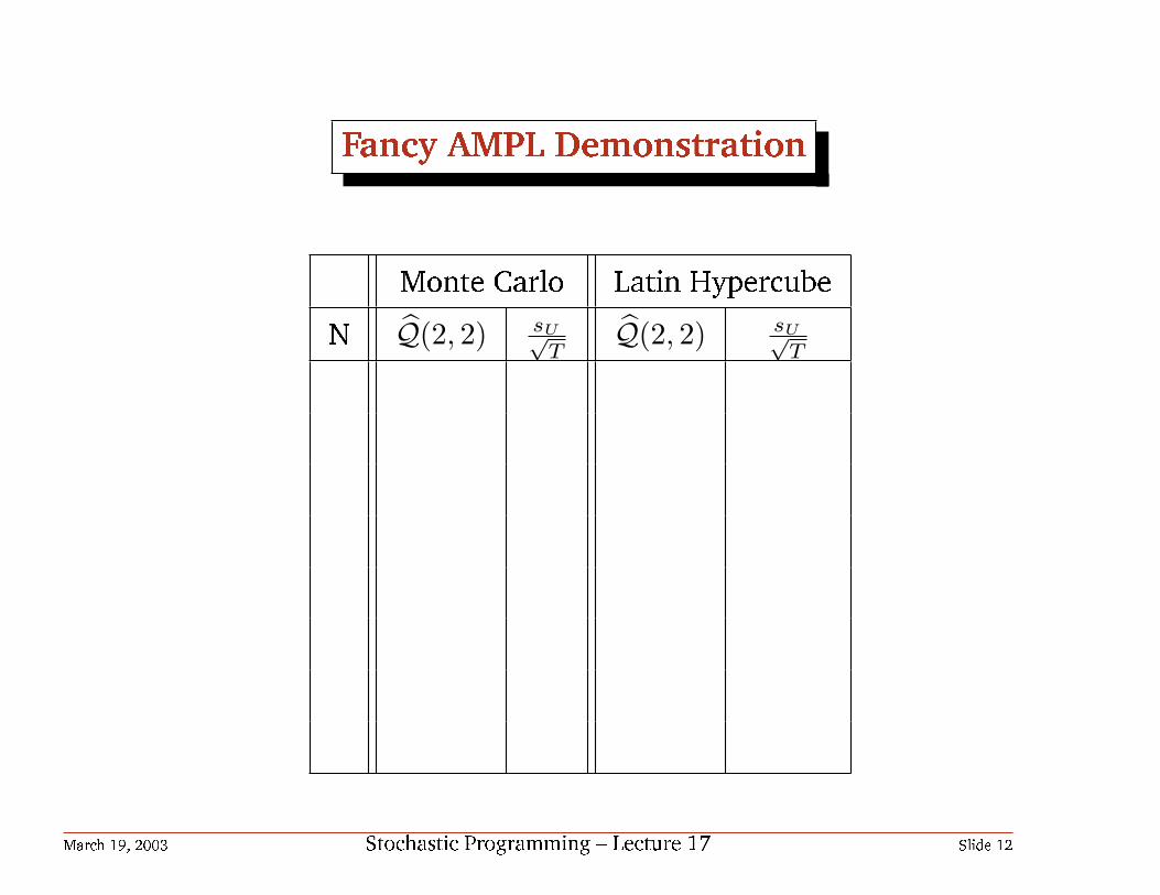
Fancy AMPL Demonstration

Monte Carlo Latin HypercubeN Q(2, 2) sU√

TQ(2, 2) sU√

T


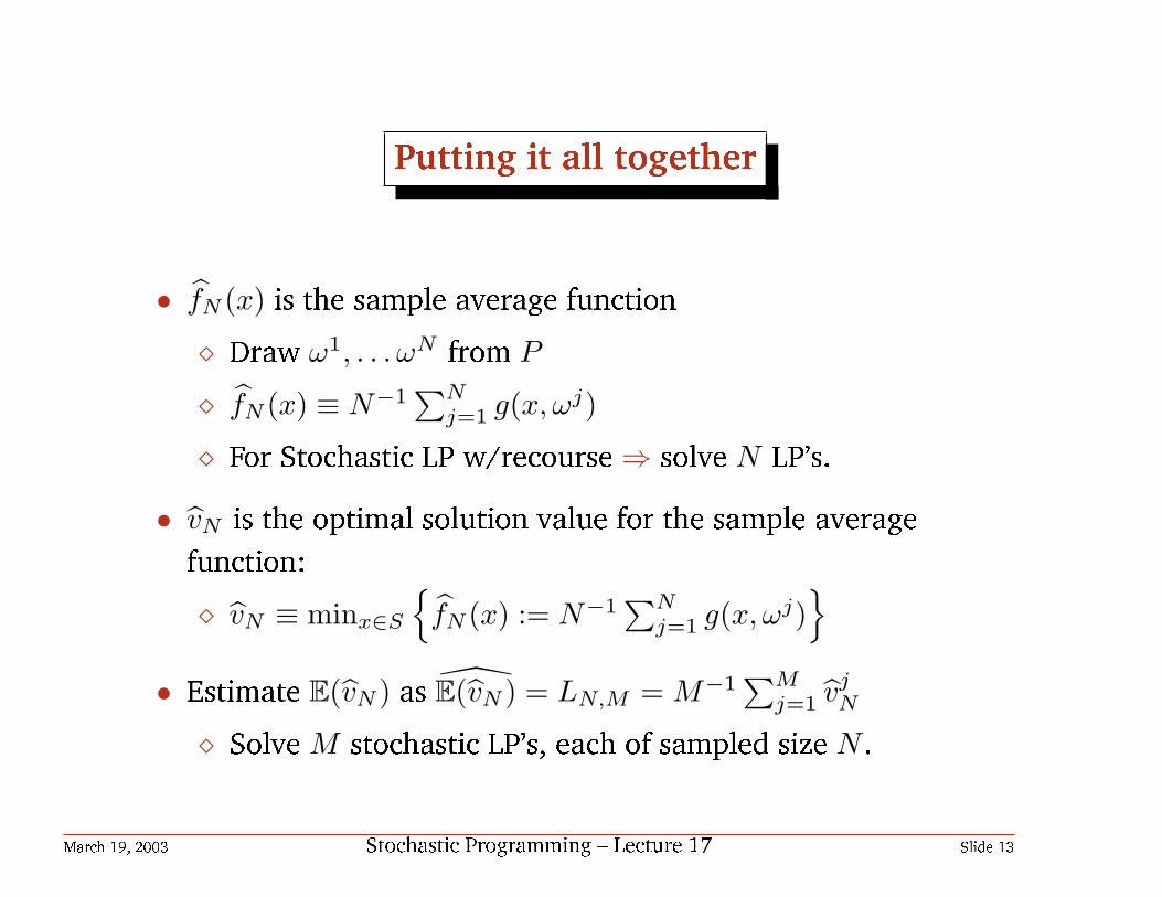
Putting it all together

• fN (x) is the sample average function¦ Draw ω1, . . . ωN from P

¦ fN (x) ≡ N−1∑N

j=1 g(x, ωj)

¦ For Stochastic LP w/recourse ⇒ solve N LP's.

• vN is the optimal solution value for the sample averagefunction:¦ vN ≡ minx∈S

fN (x) := N−1

∑Nj=1 g(x, ωj)

• Estimate E(vN ) as E(vN ) = LN,M = M−1∑M

j=1 vjN

¦ Solve M stochastic LP's, each of sampled size N .


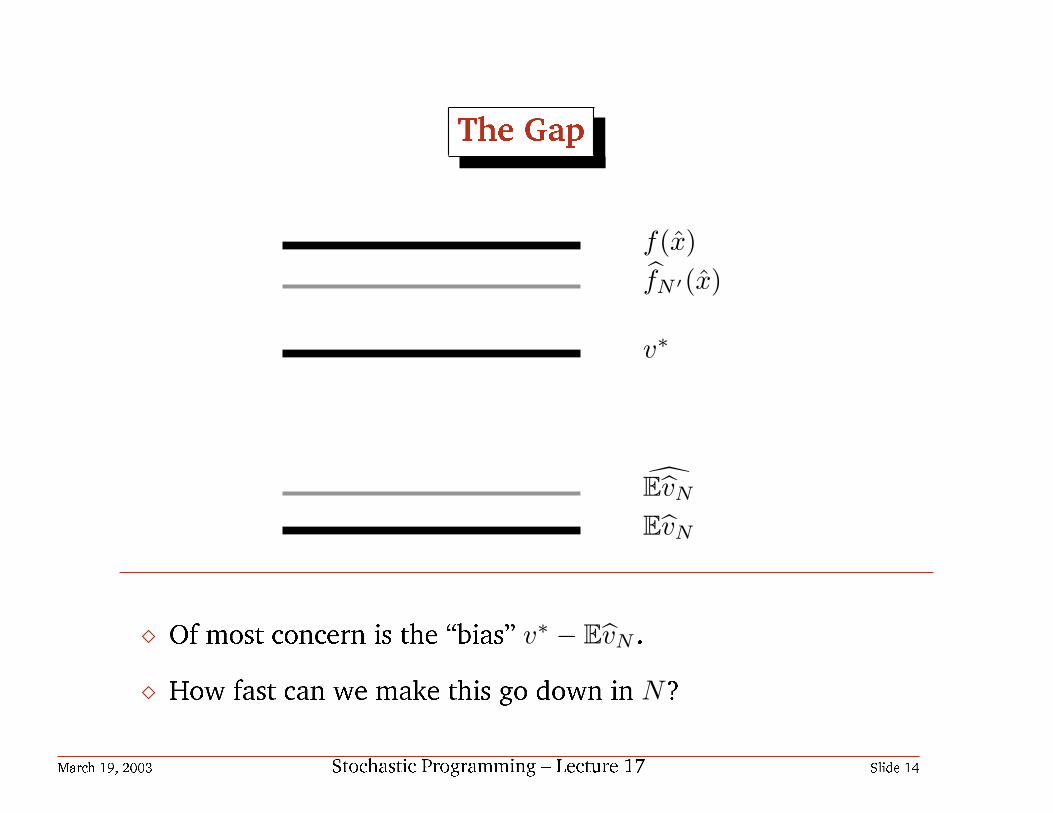
The Gap

f(x)fN ′(x)

v∗

EvN

EvN

¦ Of most concern is the bias v∗ − EvN .

¦ How fast can we make this go down in N?


A Biased Discussion

• Some problems are ill-conditioned¦ It takes a large sample to get an accurate estimate of the

solution

• Variance reduction can help reduce the bias¦ You get the right small sample


An experiment

• M times Solve a stochastic sampled approximation of size N .(Thus obtaining an estimate of E(vN )).

• For each of the M solutions x1, . . . xM , estimate f(x) by solvingN ′ LP's.

• Test InstancesName Application |Ω| (m1, n1) (m2, n2)

LandS HydroPower Planning 106 (2,4) (7,12)gbd ? 6.46× 105 (?,?) (?,?)

storm Cargo Flight Scheduling 6× 1081 (185, 121) (?,1291)20term Vehicle Assignment 1.1× 1012 (1,5) (71,102)

ssn Telecom. Network Design 1070 (1,89) (175,706)


Convergence of Optimal Solution Value

• 9 ≤ M ≤ 12, N ′ = 106

• Monte Carlo Sampling

Instance N = 50 N = 100 N = 500 N = 1000 N = 5000

20term 253361 254442 254025 254399 254324 254394 254307 254475 254341 254376gbd 1678.6 1660.0 1595.2 1659.1 1649.7 1655.7 1653.5 1655.5 1653.1 1655.4

LandS 227.19 226.18 226.39 226.13 226.02 226.08 225.96 226.04 225.72 226.11storm 1550627 1550321 1548255 1550255 1549814 1550228 1550087 1550236 1549812 1550239

ssn 4.108 14.704 7.657 12.570 8.543 10.705 9.311 10.285 9.982 10.079

• Latin Hypercube Sampling

Instance N = 50 N = 100 N = 500 N = 1000 N = 5000

20term 254308 254368 254387 254344 254296 254318 254294 254318 254299 254313gbd 1644.2 1655.9 1655.6 1655.6 1655.6 1655.6 1655.6 1655.6 1655.6 1655.6

LandS 222.59 222.68 225.57 225.64 225.65 225.63 225.64 225.63 225.62 225.63storm 1549768 1549879 1549925 1549875 1549866 1549873 1549859 1549874 1549865 1549873

ssn 10.100 12.046 8.904 11.126 9.866 10.175 9.834 10.030 9.842 9.925


20term Convergence. Monte Carlo Sampling

251500

252000

252500

253000

253500

254000

254500

255000

255500

10 100 1000 10000

Val

ue

N

Lower BoundUpper Bound


20term Convergence. Latin Hypercube Sampling

253800

254000

254200

254400

254600

254800

255000

10 100 1000 10000

Val

ue

N



ssn Convergence. Monte Carlo Sampling

2

4

6

8

10

12

14

16

18

10 100 1000 10000

Val

ue

N



ssn Convergence. Latin Hypercube Sampling

8

8.5

9

9.5

10

10.5

11

11.5

12

12.5

13

10 100 1000 10000

Val

ue

N



storm Convergence. Monte Carlo Sampling

1.544e+06

1.545e+06

1.546e+06

1.547e+06

1.548e+06

1.549e+06

1.55e+06

1.551e+06

1.552e+06

1.553e+06

1.554e+06

1.555e+06

10 100 1000 10000

Val

ue

N



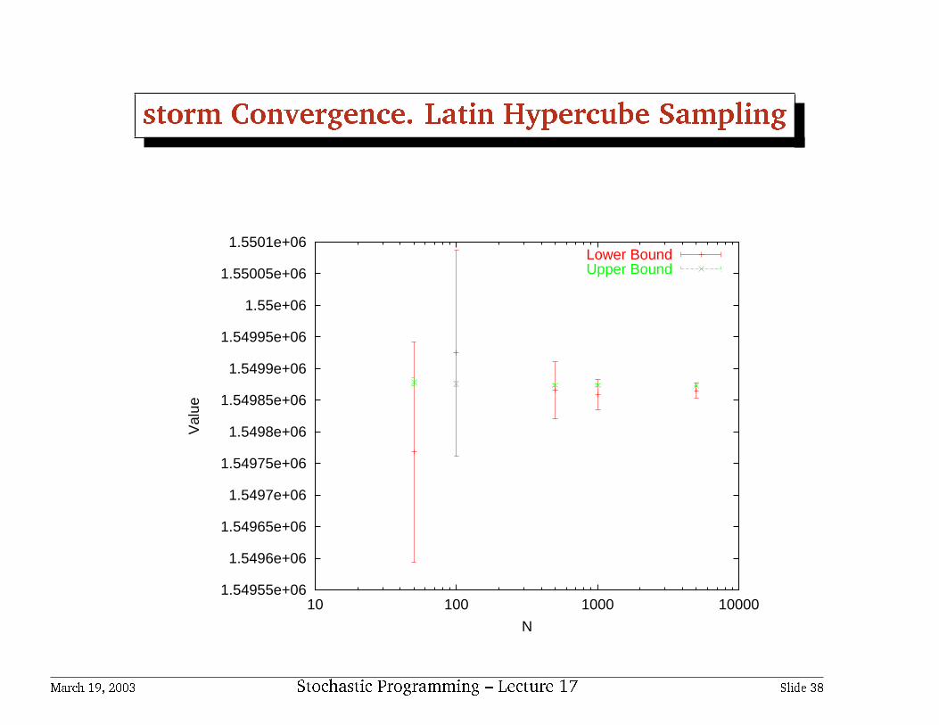
storm Convergence. Latin Hypercube Sampling

1.54955e+06

1.5496e+06

1.54965e+06

1.5497e+06

1.54975e+06

1.5498e+06

1.54985e+06

1.5499e+06

1.54995e+06

1.55e+06

1.55005e+06

1.5501e+06

10 100 1000 10000

Val

ue

N



gbd Convergence. Monte Carlo Sampling

1500

1550

1600

1650

1700

1750

1800

10 100 1000 10000

Val

ue

N



gbd Convergence. Latin Hypercube Sampling

1625

1630

1635

1640

1645

1650

1655

1660

1665

10 100 1000 10000

Val

ue

N



Convergence of Optimal Solutions

• A very interesting recent result of Shapiro and Homem-de-Mellosays the following:

• Suppose that x? is the unique optimal solution to the trueproblem

• Let xN be the solution to the sampled approximating problem

• Under certain conditions (like 2-stage stochastic LP withrecourse with nite support), the event (xN = x?) happenswith probability 1 for N large enough.

? The probability of this event approaches 1 exponentially fast asN →∞!!


Convergence of Optimal Solutions

• There exists a constant β such that

limN→∞

N−1 log[1− P (x = x∗)] ≤ −β.

• This is a qualitative result indicating that it might not benecessary to have a large sample size in order to solve the trueproblem exactly.

• Determining a proper size N is of course difcult and problemdependent¦ Some problems are well conditioned a small sample sufces¦ Others are ill conditioned


Function Shape

0

0.1

0.2

0.3

0.4

0.5

0.6

0.7

0.8

0.9

1

0 2 4 6 8 10

exp(-2*x)exp(-0.5*x)exp(-0.1*x)


Problem Conditioning

• With the help of some heavy-duty analysis, Shapiro,Homem-de-Mello, and Kim go on to give a quantitativeestimate of a stochastic program's condition.

• g′ω(x∗, d) is the directional derivative of g(·, ω) at x? in thedirection d

• f ′(x?, d) is the directional derivative of f(·) at x? in thedirection d

• The condition number κ of the true problem is

κ ≡ supd∈TS(x?)\0

Var [g′ω(x?, d)][f ′(x?, d)]2


Properties of κ

κ ≡ supd∈TS(x?)\0

Var [g′ω(x?, d)][f ′(x?, d)]2

• κ is related to the exponential convergence rate β ≈ 1/(2κ).? The sample size N required to achieve a given probability of

the event (xN = x?) is roughly proportional to κ

• If f ′(x?, d) is 0 (the optimal solution is not unique), then thecondition number is essentially innite.¦ (This is not really true).

• If f ′(x?, d) is small (f is at in the neighborhood of theoptimal solution), then κ is large

• You can also make similar statements about ε optimal solutions.


Examples

• Shapiro and Homem-de-Mello give a simple example of a wellconditioned problem where the condition number can becomputed exactly.

? For a problem with 51000 scenarios a sample of size N ≈ 400 isrequired in order to nd the true optimal solution withprobability 95%!!!

? Some real problems...

Instance |Ω| κ N≥ (95%)CEP1 216 17.45 54APL1P 1280 1105.6 3363


Distance of ssn solutions

0.00 396.72 176.90 481.92 286.11 477.05396.72 0.00 465.13 743.21 528.69 326.39176.90 465.13 0.00 501.36 381.06 495.92481.92 743.21 501.36 0.00 698.67 934.41286.11 528.69 381.06 698.67 0.00 712.62477.05 326.39 495.92 934.41 712.62 0.00

• For large sample size (N = 5000), L.H. Sampling, thesolutions xN are very far apart, even though the objectivefunctions are close to being the same.

• f(x?) is at ⇒ This instance is ill-conditioned.

• We will require a large sample size to get an ε-optimal solution


ssn Convergence. Latin Hypercube Sampling

8

8.5

9

9.5

10

10.5

11

11.5

12

12.5

13

10 100 1000 10000

Val

ue

N



Distance of 20term solutions

0.00 259.36 700.39 87504.49 77043.47 68975.66259.36 0.00 413.07 88080.16 77726.57 69723.88700.39 413.07 0.00 84761.87 74631.07 67052.76

87504.49 88080.16 84761.87 0.00 2419.97 4485.8277043.47 77726.57 74631.07 2419.97 0.00 1017.7768975.66 69723.88 67052.76 4485.82 1017.77 0.00

• This instance is also ill-conditioned


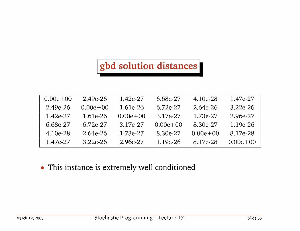
gbd solution distances

0.00e+00 2.49e-26 1.42e-27 6.68e-27 4.10e-28 1.47e-272.49e-26 0.00e+00 1.61e-26 6.72e-27 2.64e-26 3.22e-261.42e-27 1.61e-26 0.00e+00 3.17e-27 1.73e-27 2.96e-276.68e-27 6.72e-27 3.17e-27 0.00e+00 8.30e-27 1.19e-264.10e-28 2.64e-26 1.73e-27 8.30e-27 0.00e+00 8.17e-281.47e-27 3.22e-26 2.96e-27 1.19e-26 8.17e-28 0.00e+00

• This instance is extremely well conditioned


gbd Convergence. Latin Hypercube Sampling

1625

1630

1635

1640

1645

1650

1655

1660

1665

10 100 1000 10000

Val

ue

N



Distance of storm solutions

0.00e+00 3.51e-04 1.34e-05 1.11e-04 4.79e-05 5.27e-053.51e-04 0.00e+00 2.35e-04 8.94e-05 1.54e-04 1.47e-041.34e-05 2.35e-04 0.00e+00 4.73e-05 1.07e-05 1.30e-051.11e-04 8.94e-05 4.73e-05 0.00e+00 1.31e-05 1.08e-054.79e-05 1.54e-04 1.07e-05 1.31e-05 0.00e+00 1.12e-075.27e-05 1.47e-04 1.30e-05 1.08e-05 1.12e-07 0.00e+00

• This instance is also well conditioned


storm Convergence. Latin Hypercube Sampling

1.54955e+06

1.5496e+06

1.54965e+06

1.5497e+06

1.54975e+06

1.5498e+06

1.54985e+06

1.5499e+06

1.54995e+06

1.55e+06

1.55005e+06

1.5501e+06

10 100 1000 10000

Val

ue

N



Conclusions

• Sometimes theory and practice do actually coincide

• You don't need to solve the whole problem or consider allscenarios!¦ Using sampled approximations, you can quickly get good

solutions (and bounds) to difcult stochastic programs¦ Variance reduction techniques will be very helpful¦ For rare event scenarios, likely importance sampling is the

way to go


Next Time

• Interior Sampling Methods¦ Stochastic Decomposition


Documents

Sampling Methods for Stochastic Programming - …homepages.cae.wisc.edu/~linderot/classes/ie495/lecture17.pdf · IE 495 Lecture 17 Sampling Methods for Stochastic Programming Prof