ORIGINAL PAPER

Sampling density and spatial analysis: a methodological pXRF studyof the geochemistry of a Viking-Age house in Ribe, Denmark

Pernille L. K. Trant1,2 & Søren M. Kristiansen1,2& Anders V. Christiansen1

& Barbora Wouters2,3,4 & Søren M. Sindbæk2

Received: 17 February 2020 /Accepted: 23 November 2020# Springer-Verlag GmbH Germany, part of Springer Nature 2021

AbstractThis study explores the significance of spatial sampling resolution on portable X-ray fluorescence (pXRF) analysis of anarchaeological settlement site with favorable preservation conditions and clearly defined stratigraphic contexts as a benchmarkstudy to interpret geochemical mapping of anthropogenic elemental markers. We present geochemical elemental mapping of aViking-Age house floor in Denmark based on an unprecedented sampling density of a 0.25-m grid. In order to establish a fast,cost-efficient, comparable approach of how different sizes of data resolution affect the spatial elemental patterns, the data isanalysed using three different grid sizes: 0.25 m × 0.25 m, 0.5 m × 0.5 m, and 1.0 m × 1.0 m. We analysed each grid size withselected anthropogenic markers (CaO, Cu, P2O5, and Sr) using ordinary kriging. The CaO, P2O5, and Sr patterns display a stronginter-correlation between data points up to a distance of 1–1.5 m from one another. At the highest resolution (0.25-m grid), all ofthe elements display a high degree of detail in the variation of the elements across the indoor surface with low standard deviations.Hence, the precise position of hot and coldspots, and spread of bounded concentration zones, is easily recognized in the maps.With the low resolution (1.0-m grid), the borders between high and low concentrations become more blurred and the indicationsof smaller hotspots (possible activity areas) are completely lost. Especially, Cu displays a high degree of clustering, which thehigh-resolution sampling could best reveal. This benchmark study shows that it is realistic to perform large-scale geochemicalsurveys of archaeological settlements using pXRF spectrometry in a standard archaeological excavation context, but also thatsampling distances of 0.5 m × 0.5 m or finer are best suited to in indoor contexts.

Keywords VikingAge . Urbanisation . Indoor activity . Sampling design . Geochemistry . Anthropogenic elemental markers

Introduction

The organization and use of space in domestic contexts hasbecome a central topic in archaeological investigations as away of exploring activities and organization of families andhouseholds in past societies (e.g. Cook et al. 2014; Crabtreeet al. 2017; Croix 2015; Macphail et al. 2016; Milek 2012;Milek et al. 2014; Rondelli et al. 2014; Smith et al. 2001;

Sulas et al. 2019). Recent studies have approached these is-sues through the spatial distribution of artefacts or ecofacts,and increasingly also geoarchaeological methods includingmicromorphology (e.g. Barrett et al. 2007; Milek 2012;Milek and Roberts 2013; Milek and French 2007; Save et al.2020; Skre 2007). Activities can also be recognized by anthro-pogenic elemental signatures in soil geochemical maps(Woodruff et al. 2009). Case studies have shown conclusiveevidence of the correlation between elemental signatures andthe use of domestic space in ethnographic contexts (e.g. Doreand Varela 2010; Rondelli et al. 2014). Much further work isnevertheless needed to understand how geochemical signa-tures are captured, combined, and preserved in archaeologicalcontexts.

On in situ surfaces, even ancient human activity will leavechemical traces or disturbances as either an enrichment ordepletion of the geochemical signature in the substrate, as longas the floor is not entirely impermeable (Mikołajczyk andMilek 2016; Pîrnău et al. 2020; Save et al. 2020; Sulas et al.

* Pernille L. K. Trantpernille@trant.dk

1 Department of Geoscience, Aarhus University, Aarhus, Denmark2 Centre for Urban Network Evolutions, Aarhus University,

Aarhus, Denmark3 Research Foundation Flanders – FWO, Brussels, Belgium4 Maritime Cultures Research Institute, Vrije Universiteit Brussel,

Brussels, Belgium

Archaeological and Anthropological Sciences (2021) 13:21 https://doi.org/10.1007/s12520-020-01243-7

2019). In this case, the geochemical signal will be recorded inthe occupation deposits formed, and can thus be detectedusing different geochemical methods. Previous studies haveapplied different geochemical methods to measure fluctua-tions in element concentrations across a surface and presentedthe results as isopleth maps (e.g. Milek and Roberts 2013;Milek et al. 2014). However, as noted by Dore and Varela(2010) this approach has limitations regarding the interpreta-tion of use of space and visualization of the geochemical data(Dore and Varela 2010). Thus, Dore and Varela (2010) sug-gested a new approach for spatial analysis of multivariatedatasets using interpolation methods. This was applied withsome modifications, to an outdoor area on a farmstead inIceland by Mikołajczyk and Milek (2016), and revealed dif-ferent activity areas providing information about the function-al character and evolution of each area.

Traditionally, laboratory methods such as inductivelycoupled plasma atomic emission spectroscopy (ICP-AES) ormass spectroscopy (ICP-MS), loss on ignition (LOI), magnet-ic susceptibility, and X-ray fluorescence (XRF) have beenused to study changes in elemental concentrations at archae-ological sites (e.g. Cook et al. 2014; Linderholm 2007;Macphail et al. 2004; Milek and Roberts 2013; Milek et al.2014; Sulas et al. 2019; Wilson et al. 2005, 2008). Morerecently, quicker and more cost-efficient methods that replacewet chemistry for the analysis of soil elements and permitlarge-scale routine soil mapping, such as portable X-ray fluo-rescence (pXRF), have been included in pedogenesis andgeoarchaeological studies (e.g. Abrahams et al. 2010; Horáket al. 2018; Lubos et al. 2016; Mikołajczyk and Milek 2016;O’Rourke et al. 2016; Pîrnău et al. 2020; Save et al. 2020;Šmejda et al. 2018; Stockmann et al. 2016). As a result, thismethod has been recognized as an effective tool for soil anal-ysis in studies of pedogenesis (Stockmann et al. 2016) andmapping of the use of space in archaeological contexts(Fleisher and Sulas 2015). Other handheld instruments, suchas laser-induced breakdown spectroscopy (LIBS), magneticsusceptibility, and visible near- and mid-infrared spectroscopy(vis-NIRS and MIRS), are also developing fast in adjacentsciences (Nicolodelli et al. 2019; Zhao et al. 2019), and arepromising tools for supporting on-site archaeological interpre-tation, either as stand-alone methods, in combination withpXRF, or together with geophysics (Cannell et al. 2018;Fleisher and Sulas 2015).

The application of fast methods such as pXRF also offersthe opportunity to apply thorough spatial geostatistical analy-ses (e.g. Fleisher and Sulas 2015; Lubos et al. 2016; Pîrnăuet al. 2020; Rondelli et al. 2014; Thompson et al. 2018).Geostatistical estimation and interpolation such as kriging,which includes spatial data variation, allows for detailed stud-ies of correlation between parameters as well as the uncer-tainties introduced by interpolation to provide unbiased esti-mates with minimum variance (Oliver and Webster 2014). A

key part of kriging is modelling of the semivariogram, whichis a measure for the spatial dependencies and structures arisingfrom the underlying spatial variation held in the data. Krigingis then applied to predict values of a given soil parameter inunsampled locations using the semivariogram model(Entwistle et al. 2007; Webster and Oliver 1990). Kriging isthe most widely applied technique for geostatistical modellingof spatial contexts, and different kriging methods have differ-ent potential in predicting the spatial variability (Rondelli et al.2014). The method is not yet widely applied to archaeologicalsites, but several studies have already demonstrated its poten-tial (e.g. Cook et al. 2005; Entwistle et al. 2007; Haslam andTibbett 2004; Wells et al. 2007; Wells 2010).

It is well known that the archaeological record includestraces of human activities in the sediments’ elemental compo-sition. However, there is a general lack of studies regardingthe spatial resolution to which we can study small-scale vari-ations in elemental concentrations across indoor areas. Themethodology for investigating activity areas based on geo-chemistry has recently further been developed andestablished in work conducted by Dore and Varela (2010)and Mikołajczyk and Milek (2016). Some anthropogenic ele-ments might only be correlated to one or two activities (e.g.Sulas et al. 2019), and as a result the corresponding elementalpattern can be limited in extent and, thus, might display ahotspot tendency. Here, a hotspot is considered to be a smallcollection of samples with concentrations much higher thanthe mean, i.e. Cu at > 50% mean in this study. Detection ofsuch indoor hotpots needs to be evaluated in terms of itsrecognisability as a result of the sampling density, as humanindoor activities leave behind different soil patterns comparedto e.g. stabled animal husbandry (Macphail et al. 2004).

Our aim is to study the optimal sampling resolution basedon pXRF elemental measurements on a site with relativelyfavorable indoor preservation conditions and clearly definedstratigraphic contexts as a benchmark study to understandgeochemical investigations in less well-preserved settings. Indoing so, this methodological study thus evaluates how dif-ferent sampling densities (meaning different resolutions ofsampling grids) affect the visualization of the spatial distribu-tion of elements across an indoor surface, and how dense thesampling should be for the samples to be statistically correlat-ed. An additional rationale is a cost-efficient application withan increased potential use in daily routine fieldwork in a con-text of developer-funded archaeology.

Materials and methods

Study area

The trading town or emporium Ribe (Fig. 1) emerged in theearly 8th century as a part of the maritime trading network in

21 Page 2 of 17 Archaeol Anthropol Sci (2021) 13:21

the northern Wadden Sea (Croix 2015). By the end of the 8thcentury, it had grown into a dense, permanent settlement withtwo parallel rows of plots with wattle houses, divided by anarrow street and ditches in-between. Together with tradingactivities, the site housed a range of specialist crafts includingcopper-alloy metalworking (Croix 2015; Feveile 2006, 2012;Feveile and Jensen 2000; Jensen 1991).

Ribe is located approximately 5.5 km inland at a pointwhere a dry, sandy Ice Age hill island meets the marshlandof the Wadden Sea coast (Fig. 1). During the Viking Age,Ribe was accessible by ship from the Wadden Sea on thestream Ribe Å (Feveile 2010). The Viking-Age part of Ribesouth of the stream is placed on a small outwash bank ofglacial age (Mertz 1977) covered by aeolian sand depositedaround 2000 BP (Dalsgaard 2005). The marshland west of thetown provides grazing areas for livestock (Mertz 1977) andpotentially clay as building materials.

During 2017 and 2018, the Northern EmporiumExcavation Project conducted a full stratigraphic excavationof a central part of Viking-Age Ribe (Sindbæk 2018). Theexcavation was located at what is today known as“Posthustorvet” (the area between the Art Museum, Sct.Nikolaj Gade 10, and the former Post Office) in the centreof modern-day Ribe and close to earlier excavations (see

Feveile 2006; Sindbæk 2018). The excavation covered almostthe full extent of one building plot (Plot 1), including ditcheson both sides, the front part of the opposite plot (Plot 2), andthe street separating both plots. On Plot 1, the excavationuncovered several clay layers belonging to different succes-sive buildings and activity phases from the earliest stages ofthe settlement. The clay layers seem to reflect ‘passive’ floorlayers (sensu Gé et al. 1993), constructed for the purpose oflevelling and stability or the complete rebuilding of the houseson top of older structures. These clay floors, and the associatedoccupation deposits formed on top of them, can provide valu-able information about the activities that took place insidehouses at this early stage of urbanisation in Viking-AgeDenmark.

The Northern Emporium excavation of Ribe applied anexcavation strategy encompassing systematic 3D laser scan-ning, and intensive and large-scale micromorphological sam-pling as an integrated part of the excavation record (Croixet al. 2019). Similar high-definition excavation strategies areanticipated to be more widespread and an understanding ofcost-efficiency in the targeted sampling of excavation units isincreasingly important for archaeological field practices.

To test the application of high-resolution multi-proxy anal-yses for the use of urban spaces, we chose to target an

Northern Emporium Excavation

Earthworks

200 mN

MarshGrassland plainMoorland plainGlacial sandMorainChurches

from the Viking Age/Medieval Age

Ribe

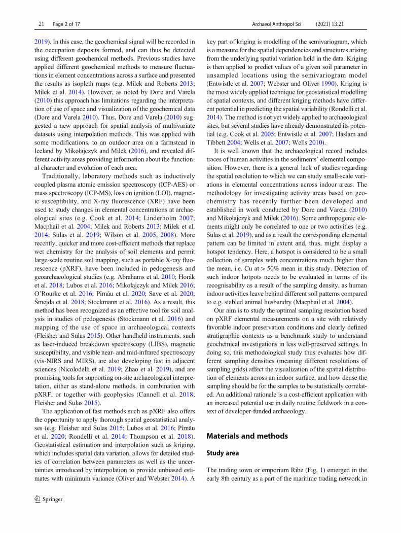
Fig. 1 Left: Reconstruction of the townscape of Ribe’s emporium in theViking Age. The red circle marks the approximate location of theNorthern Emporium Excavation. The market site (from ca. 700 ADonwards) is represented by two rows of parallel plots on either side of amedian street. The earthworks only appear after the middle of the ninth

century. The grave field to the east was mostly in use in the eighth andearly ninth centuries. Graphics: Morten Søvsø and Louise Hilmar. Right:The geology of the southwestern part of Denmark with the location ofRibe and important findings from the Viking Age in the area. Modifiedafter Feveile (2010)

Archaeol Anthropol Sci (2021) 13:21 Page 3 of 17 21

archaeologically interpreted indoor occupation deposit withthorough sampling for geochemistry along a dense grid. Thesubsequent excavation showed that most of the sampled layersbelonged to the upper phase of the house designated as “K22”,but due to indistinctness in the stratigraphy, some limitedareas contain remains from the lower phase of a youngerhouse “K23” comprising a workshop for non-ferrous metal-working recognized during excavation (Fig. 2). Difficulties inseparating different layers of clay arose from the sinking anddeformation of the stratigraphy due to underlying features richin organic matter. The sampled floor layers measure approx-imately 7 × 10 m, and are radiocarbon dated to the period c.780–820 CE (Philippsen et al., in prep.).

The targeted occupation deposits (Figs. 2 and 3) oc-curred in the excavation as thin, dark-brown layers witha thickness varying from a few millimeters to a couple ofcm directly overlying the clay floors. Table 1 includes thefull description of recognized excavation units. On-site,two side aisles, a middle aisle, and two front rooms weredistinguished according to differences in sediment colourand texture.

The main part of the targeted occupation deposits belongto house K22 phase c. K22c includes the following strati-graphic units: lowermost are the clay floors defining theoutline of the house (excavation units A280–A283 andA285, see Fig. 2), a collapsed baking oven (i.a. A276) andactivity, sand and ash layers (among others A262 andA263). Of these excavation units, only the occupation de-posits A262 and A263, the hearth A273, and the bakingoven A276 were sampled for geochemistry (Fig. 3).

At the time of sampling, K22c was disturbed by youngerfeatures from the lowermost phase of house K23 (excavationunits A264 and A273). House K23 consists of a sequence oflayers including among others its lowermost clay floors, ahearth, and two occupation deposits. From K23, only one ofthe occupation deposits (A264) and the hearth (A273) wereincluded in the sampling.

In addition to the layers from within house K22c and K23,the sampling also covered an outdoor area (A266) south of thehouse interpreted as a shallow ditch or pathway, whichcontained large amounts of animal bones in a dark homoge-neous matrix, as well as part of the road northeast of the house(A243) which was observed as dark sediment with a patch oflight sand (A265, see Fig. 3).

Sampling and sample preparation

Undisturbed sediments from the two houses, K22c and K23and adjacent shallow ditch, road, and back area, were bulksampled across the entire surface along a 0.25-m × 0.25-mgrid (Fig. 3a). Due to post-depositional processes, the sitewas significantly sloping towards the side aisles and ditches.As a result, an artificial horizontal grid was projected onto thesloping surface using coordinates and a Trimble SX10(DGPS) high-density 3D laser scanning total station. On everygrid point, a skewer was placed to mark the intersections, andsub-cm precise, real-time coordinates of each sample in thegrid were recorded. All sediment samples were taken up to a10-cm radius around each grid point and care was taken not toinclude any underlying layers. Sampling bias was minimized

Fig. 2 House phase K22c with disturbance from house K23 (occupationdeposit A264 and the sunken feature hearth A273). House phase K22c isdefined by the clay floors A280–A283 and A285. The sampled

occupation deposits A262 and A263 that overlie the clay floors and thebaking oven A276 are also shown. The shown house phase was radio-carbon dated to the period c. 780–820 CE

21 Page 4 of 17 Archaeol Anthropol Sci (2021) 13:21

by securing that all samples were collected by the same indi-viduals during three days only. Each bulk soil sample weighedapproximately 150 g and was numbered according to the grid.In total, 1059 bulk samples were collected.

All 1059 samples were air dried at low temperature (ap-proximately 27 °C), gently powdered with a ceramic mortarand pestle and 2-mm dry sieved to remove any components> 2 mm. Finally, approximately 30 ml of each sample wasrepresentatively subsampled making sure all size fractionswere included, ground using a Retsch RS200 to ensure homo-geneity, and stored in medicine glasses.

Laboratory analyses

All 1059 soil samples were analysed in the laboratory using astandardized set-up and a Bruker S1 Titan 800 portable XRFscanner with an Rh anode tube and a maximum voltage of 50kV/39 μA. The instrument works with a collimation standard of5 mm and a five position motorized filter changer. For the anal-yses, the chosen application was the mining mode “GeoChem”with method “GeoChem General”, which includes full supportfor light elements through dual phase measurements. Precedingthe main analysis, a reference sample with known elementalvalues was measured several times in order to choose the phasesettings that gave the best replication with shortest exposuretimes. Based on this, the phase settings were selected to 30 sfor both the first and second phase. The reference sample was

measured in between samples to account for possible drifting inthe instrument. Each sample was analysed three times and theresulting mean of each element was used.

Samples were analysed for 38 different elements as standard.From these, four elements (calcium, copper, phosphorus, andstrontium) were selected for further study. These elements wereselected since they are already known as indicators of differentindoor activities (Milek andRoberts 2013; Sulas et al. 2019). Therationale for selecting four elements only in this methodologicalstudy is that they cover the overall variations expected from bothnatural and anthropogenic sources (e.g. Sulas et al. 2019). First,phosphorus is found to be the best ethnographic and archaeolog-ical indicator in most geochemical studies and is associated witha variety of sources, such as foodstuffs in general, dung, marinefoodstuffs, household waste, middens, and hearths (Mikołajczykand Milek 2016; Milek and Roberts 2013; Sulas et al. 2017;Sulas et al. 2019). Next, copper is a tracer of metalworking butalso household waste, middens, and hearths (Fleisher and Sulas2015; Sulas et al. 2017, 2019). Calcium and strontium are poten-tial indicators of the texture and the mineralogical assemblageassociated with the variations in the parent soil materials in thelocal, naturally acidic soils, but in these purely anthropogenicdeposits they should be regarded as anthropogenic markers fore.g. plant nutrients and bone (foodstuffs in general), wood ash,general household waste, middens, and hearth deposits (Cooket al. 2014; Fleisher and Sulas 2015; Mikołajczyk and Milek2016; Milek and Roberts 2013; Sulas et al. 2017, 2019). The

Table 1 Description of excavation units recognized on-site from house K22c and K23

Unitno.

Thickness Description Interpretation

A262 5–7 cm Heterogeneous mixture of greyish brown sand rich in organic matter; and greenish clayey silt.Boundaries range from sharp to diffuse. Moderate to strong bioturbation. Inclusions ofsmaller flint gravel within the sand.

Activity deposit in K22 phase c

A263 3–5 cm As A262 Activity deposit in house K22phase c

A264 Lamination of predominantly orange-coloured sand; grey silty clay with temper of horizontallybedded organic matter and traces of organic bedding (woven grass or hay/straw); andcharcoal-rich sand. Inclusions of large burnt clay and/or daub aggregates, glass slag, cal-cined bone (up to 5 cm), metal finds, and a metal-filled crucible. Wavy to somewhat diffuseboundaries.

Activity deposit in house K23

A273 5–10 cm Homogeneous, orange-red, compacted clay with traces of burning and hardening at the verytop.

Hearth in house K23

A276 10–12 cm The bottom level consisted of greenish-yellow unburnt clay. In the middle was a distinctsurface of yellow to orange clay with traces of burning. The top was represented by a5-cm-thick layer yellow to orange clay with traces of burning and a lumpy, but still compactstructure.

Remains of collapsed baking ovenin house K22 phase c

A280 0–5 cm Two thin, homogeneous, greenish-yellowish silty clay layers separated by a thin, dark-brownsand layer containing ash.

Part of clay floor in house K22phase c

A281 0–5 cm Porous, homogeneous red to orange silty clay of varying thickness, thinnest in the middlewhere the layer was almost worn away in some places.

Part of clay floor in house K22phase c

A282 0–5 cm A homogenous, only sporadically preserved, yellowish grey, thin, silty clay. Part of clay floor in house K22phase c

A283 0–5 cm A lamination of several thin, homogeneous yellowish grey silty clay layers separated by thindark-brown sand layers containing organic matter and ash.

Part of clay floor in house K22phase c

Archaeol Anthropol Sci (2021) 13:21 Page 5 of 17 21

archaeological interpretation of the full set of elements in our gridhas to be based on a multi-scalar, multi-method approach and isthus not discussed here.

No natural reference material analyses are included in thispaper. Since (a) the main aim is to discuss relative enrichment

patterns vs. sampling grid size, and (b) as the EuropeanGEMAS project data (Reimann et al. 2018) are derived fromagricultural and from grassland soils, which in Denmark sharethe same intensive land use history for > 200 years with addi-tion of lime, marl, inorganic fertilizers, and slurry (Pedersen1995; Schjonning et al. 1994; Westh 1909), the expectationthat grassland represents natural soil properties is highly un-certain. Archaeologically, relevant natural, undisturbed soilsappear to be extremely rare in Denmark outside protectedheathlands and ancient woodlands (Kristiansen andDalsgaard 2000; Nielsen et al. 2019; Thomsen andAndreasen 2019), and no heathlands nor ancient woodlandsare found on comparable parent materials surrounding Ribe.

Geostatistical analyses

In order to compare how different data sampling densities affectthe spatial elemental patterns, two new grids were created basedon the original 0.25-m × 0.25-m sample grid, creating in totalthree grids: 0.25 m × 0. 25 m, 0.5 m × 0.5 m, and 1.0 m × 1.0 m(hereafter denoted 0.25-m, 0.5-m, and 1.0-m grid, respectively).For each grid size, each element (CaO, Cu, P2O5, and Sr) wasanalysed on its own. Descriptive statistics of elemental dataconstituting the three different grid resolutions are shown inTable 2. No transformation was applied to the data prior tokriging, and the individual data points were computed as thearithmetic mean of the three measurements per sample.

The spatial analyses were conducted using ordinary kriging inthe software program “R” version 3.4.3 with the following add-on packages: sp, gstat, and raster; see Pebesma (2004, 2014) fordetails on kriging using the gstat package in R. A key part of thekriging procedure is the estimation of the so-calledsemivariogram. In the R-package, modelling of the different pa-rameters (model, sill, range, and nugget) is allowed when fittingthe semivariogram model. In turn, the semivariogram model isused for calculating the predicted (kriged) elemental concentra-tions, which are then shown as surface covering maps of thedifferent elements as the output. Eachmap of predicted elementalconcentrations is accompanied by a map of the standard devia-tion (% points) of the predicted values (weight %).

The semivariogram describes half of the mean variancebetween all possible point-pairs in the dataset as a functionof distance or lag. The semivariogram values, γ, for the sam-pled parameter z are calculated at regular lags, h, as describedbelow (Pebesma 2014):

γ hð Þ ¼ 1

2N∑N

i¼1 zi−ziþh½ �2 ð1Þ

where N is the number of pairs within the given lag inter-val, h; zi is the measurement of the regionalized variable takenat location i; and zi + h is another measurement taken h lagintervals away.

Fig. 3 Location of the three grids applied, a 0.25 m × 0.25 m, b 0.5 m ×0.5 m, and c 1.0 m × 1.0 m and all sampled excavation units. The sampledexcavation units cover the occupation deposits (A262 and A263) and thebaking oven (A276) from house phase K22c with disturbance from anoccupation deposit (A264) and the sunken feature hearth (A273) fromhouse K23. Part of the road (A243 and A265) and the southern ditch(A266) were also covered by the geochemistry sampling

21 Page 6 of 17 Archaeol Anthropol Sci (2021) 13:21

In order to obtain comparable results, modelling of thesemivariogram parameters was based only on the 0.25-m griddataset, since this sampling density contains spatial informa-tion starting from 0.25 m, but includes all the information onthe 0.5 and the 1.0 sampling scale. Hence, for sampling dis-tances over 1.0 m, the semivariograms should theoretically bethe same and the observed differences arise because we havefewer data for the coarser grids and hence a more uncertainrepresentation of the underlying true spatial statistics. The0.25 fitted variogram model was therefore applied for theprediction maps of the 0.5-m and 1.0-m grids as well. Theprediction grids for all cases are set at a 2-cm resolution toensure that all relevant spatial details are captured.

We decided to fit the semivariogram model manually asopposed to automatic fitting with, for instance, a non-linearinversion. The rationale behind this is that it was prioritized tofit the first 2–3 data points (meaning up to a distance of 0.75 m)as well as possible, even though this might compromise thefitting for the data points on a larger distance. This approachwas chosen because the semivariograms (Fig. 4) mainly displaycorrelation up to around 1 m, while no or very little correlationexists between data points of a greater distance. Correlationbetween samples is a necessity for meaningful predictions ofelemental concentrations in-between samples. The fittedsemivariogram model parameters can be found in Table 3.

Results

Semivariograms

The semivariograms (Fig. 4) inform us about the spatial cor-relation of the measured data values in the grid points. Thepoints are the experimental semivariance values and the solidline displays the fitted semivariogram model based on the0.25-m grid points. When the experimental semivariances

are small, the data are strongly correlated at that distance andvice-versa for large semivariances. When the semivariogramflattens out, the correlation becomes smaller and approaches avalue linked to the variance of the mean of all samples.

For three of the elements (CaO, P2O5, and Sr) and two ofthe grid resolutions (0.25 m and 0.5 m) (Fig. 4), thesemivariograms show a steep slope up to a distance of 1–1.5m. Hence, the CaO, P2O5, and Sr sample values are correlatedwithin a 1–1.5-m distance from one another. Beyond 1.5 m,the elements loose their correlation. Thus, at a distance greaterthan 1–1.5 m, the sample points no longer provide usefulinformation for the prediction of the elemental concentration.

The semivariograms (CaO, P2O5, and Sr) for the lowest res-olution grid (1.0 m) do not display the same degree of correlationbetween sample points as the two higher resolution grids (0.25mand 0.5 m). This tendency is due to the resolution of thedataset—all correlated information lies within a distance of 1 m.

Prediction of elemental concentrations and theiruncertainties

Figures 5, 6, and 7 show both the predicted elemental concen-trations and the standard deviation on the predicted values forCaO, P2O5, and Sr respectively. In the following, we willevaluate and compare the results visually. In the highest reso-lution (0.25-m grid), all of the elements display a large degree

Table 2 Descriptive statistics of elemental data (%) for all three grid resolutions

Element No. of samples Min Max Mean Standard deviation

CaO (0.25 m) 1059 0.742 12.984 3.593 1.270

Cu (0.25 m) 1059 0.002 1.116 0.042 0.068

P2O5 (0.25 m) 1059 0.840 9.821 3.693 1.164

Sr (0.25 m) 1059 0.007 0.059 0.026 0.006

CaO (0.5 m) 277 0.835 10.711 3.549 1.308

Cu (0.5 m) 277 0.004 0.432 0.040 0.058

P2O5 (0.5 m) 277 0.916 9.020 3.590 1.160

Sr (0.5 m) 277 0.011 0.059 0.025 0.006

CaO (1.0 m) 74 1.213 10.711 3.603 1.624

Cu (1.0 m) 74 0.005 0.325 0.035 0.054

P2O5 (1.0 m) 74 1.081 9.018 3.618 1.365

Sr (1.0 m) 74 0.011 0.059 0.026 0.008

Table 3 Model parameters of the best semivariogram-fit for each ele-ment based on the 0.25-m × 0.25-m grid

Element Sill Model Range Nugget

CaO 1.56801 Spherical 1.25 0.5704163

Cu 0.006732696 Exponential 2 0.0007280126

P2O5 1.419789 Exponential 0.7 0.3056974

Sr 4.133472e−05 Exponential 0.7 1.207976e−05

Archaeol Anthropol Sci (2021) 13:21 Page 7 of 17 21

of detail in the behaviour of the elements across the surface.The borders between high and low concentrations are alsovery clear; hence, the precise position and spreading of bound-ed concentration zones are easily recognized in the graphics.The 0.25-m grid resolution also displays low standard devia-tions between data points across the entire surface for CaO,P2O5, and Sr. The low standard deviation of the predictedconcentrations indicates that this resolution is very well suitedfor prediction of precise elemental concentrations and, thus, aprecise indication of the location of different possible indooractivity areas.

For the 0.5-m grid, the predicted elemental concentrationsstill show the location of areas with high and low concentra-tions relatively precisely, but the smaller areas are lost and thesignal is more unclear. For the 0.5-m grid resolution, the stan-dard deviations of the predicted elemental concentrations be-come larger than for the highest resolution; thus, the predictedmaps are somewhat less accurate.

When the lowest resolution (1.0-m grid) is compared tothe highest resolution (0.25-m grid), it is clear that thelow-resolution dataset only shows main trends in the pre-diction of the elemental concentrations. With the low res-olution, the borders between high and low concentrationsbecome more blurred and the indications of smaller(possible) activity areas are completely lost. This lowerresolution prediction is also followed by larger standarddeviations when moving away from the observationpoints, and, hence, predicted values far from an observa-tion point are more uncertain than the ones predicted bythe highest resolution data set (0.25 m). In addition, sincethe semivariances on the 1.0-m grid (Fig. 4) are larger, asemivariogram model fitted to the 1.0-m grid instead ofthe 0.25-m grid would yield even larger uncertainties onthe predicted concentrations. As the semivariograms inFig. 4 demonstrate, the data values do not display corre-lation at a distance beyond 1–1.5 m. This also shows that

Fig. 4 Semivariograms showing the spatial correlation for CaO, Cu, P2O5, and Sr in the three grid resolutions (respectively 0.25 m × 0.25m, 0.5 m × 0.5m, and 1.0 m × 1.0 m) and the fitted models

21 Page 8 of 17 Archaeol Anthropol Sci (2021) 13:21

the low-resolution data do not produce reliable predictionmaps since the data points are on the outer limit of infor-mation about the neighboring data points. Another obser-vation is that because the semivariograms indicate rough-ly the same spatial correlation lengths across the differentelements, the uncertainty maps on the predictions are very

similar. If, for example, one of the semivariograms hadbeen flatter with smaller values (i.e. less spatial variation),the uncertainty maps would have revealed smaller uncer-tainties moving away from an observation point.

Two features, “A” and “B”, are marked in Figs. 5, 6,and 7, showing potential activity zones not recognized

Fig. 5 Predicted surface elemental concentrations and variance on the predictions for CaO in the 0.25-m × 0.25-m grid (a and b), 0.5-m × 0.5-m grid (cand d), and 1.0-m × 1.0-m grid (e and f)

Archaeol Anthropol Sci (2021) 13:21 Page 9 of 17 21

during excavation. Feature A is an area of approximately1.5 × 0.5 m crossing the central aisle with elevated ele-mental concentrations. With the high resolution (0.25 m),this feature is very distinct in all predicted maps of CaO,P2O5, and Sr. When the resolution is decreased to the 0.5-m grid, the feature becomes less evident and with the

lowest (1.0 m) resolution, it is no longer possible to rec-ognize this area as an independent and possible activityzone. Feature B encompasses an area with depleted con-centrations of all three elements stretching approximately3 × 1.5 m along the central aisle. Feature B is most prom-inent for P2O5 and Sr, while it is somewhat less clear in

Fig. 6 Predicted surface elemental concentrations and variance on the predictions for P2O5 in the 0.25-m × 0.25-m grid (a and b), 0.5-m × 0.5-m grid (cand d), and 1.0-m × 1.0-m grid (e and f)

21 Page 10 of 17 Archaeol Anthropol Sci (2021) 13:21

the predictions of CaO. However, this seems to be due tothe surrounding higher concentration areas, which aremore pronounced for P2O5 and Sr, since concentrationsof CaO are below the mean in this Feature. As was thecase for Feature A, the high 0.25-m grid resolution clearly

demonstrates Feature B as different regarding the relativeconcentrations. When lowering the resolution, Feature Bbecomes less pronounced and with the 1.0-m grid, it isdifficult to separate this as a distinct feature with depletedconcentrations.

Fig. 7 Predicted surface elemental concentrations and variance on the predictions for Sr in the 0.25-m × 0.25-m grid (a and b), 0.5-m × 0.5-m grid (c andd), and 1.0-m × 1.0-m grid (e and f)

Archaeol Anthropol Sci (2021) 13:21 Page 11 of 17 21

Hotspots

As described in “Introduction”, some elements might onlyreflect a few different activities, and, thus, can display a“hotspot tendency”. Here, this is the case for copper andas Fig. 8 shows, the distribution of high-concentrationcopper is restricted to the central part of the western sideaisle belonging to house K23, marked as Feature “C”.Elsewhere, the concentration is very low, with only smallcopper accumulations spread across the eastern part of thehouse.

With the high-resolution dataset (0.25-m grid), the pre-cise extent and concentration levels of Feature C can bediscerned. It is clear that the distribution of the highestcopper concentrations is very limited in extent, but thatthese are supported by high Cu-concentrations northeastof the hotspot. As the grid resolution is lowered (0.5-mgrid), the hotspot area appears larger in extent and thevery high copper concentrations in the centre of thehotspot are lost. The low-resolution 1.0-m grid only pro-vides information about the area in which the hotspot islocated, and not about its actual magnitude and extent.Additionally, the smaller copper accumulations outsideof Feature C is no longer visible with the 1.0-m grid.

Discussion

How sampling density affects the outcome: fieldprotocol and geostatistics

In archaeological research, the choice of interpolation griddensity versus sampling density is a compromise especial-ly based on the state of preservation of the deposits, andthe excavation methods. The sampling density, samplingdesign, and geostatistics to interpolate the data are of par-amount importance for the interpretation of mapping ofany soil property, and we do not know a priori if thedistribution of an element represents activity patterns pre-served in situ or is biased by complex depositional andpost-depositional processes (Webster 2000). The in-creased availability of rapid, non-destructive, and simul-taneous multi-element analyses of exposed surfaces in thefield and on soil samples in the laboratory furthermorerequires good sampling practice. In our case, the hetero-geneity and error types involved in sampling and process-ing were minimized by (a) collecting small compositesamples, (b) applying representative mass reduction, (c)non-contaminating crushing, and (d) unbiased mixing be-fore subsampling, as required in good sampling of hetero-geneous materials (Esbensen et al. 2010). In Ribe’s well-defined stratigraphy, a near ideal field sampling protocolwas possible despi te s ignif icant t runcat ion and

bioturbation (see e.g. voids on Figs. 5, 6, 7, and 8). Oneven more strongly bioturbated sites, in other climatezones, or with more heavily disturbed stratigraphy, how-ever, greater difficulties are expected in this first step ofthe representative sampling. Nevertheless, the samplingdensity resulting from our clearly defined stratigraphiccontexts is very likely to be applicable in other anthropo-genic and archaeological studies of indoor contexts.

The choice of kriging for interpolation can result inlocal anomalies being smoothed out, while another sideeffect is that the interpolated data can be below or abovethe original data point(s). However, in both cases, thekriged values will be the most likely estimate as the sam-pled values are inherently uncertain as indicated by thesize of the nugget value. In the case of mapping indoorspace, this is likely of little concern in non-enriched areaswhere values cluster very much around an expected aver-age background value or larger hotspots; whereas in caseswhere only few samples are at the extremes, this type ofeffect may disturb our ability to detect very smallhotspots. Hence, close inspection of both absolute mapcolours and their standard deviation scale (Figs. 5, 6, 7,and 8) has to be considered carefully. Adding inversedistance weighting maps may help circumvent some ofthese problems, but can give rise to other, more seriousissues, such as the ‘bulls eye’ effect, where hot- andcoldspots may seem over-represented.

Considering the elemental maps of CaO, P2O5, and Srin our study, the semivariograms in Fig. 4 show that thespatial correlations level out between 1 and 1.5 m of sam-pling space. This implies that the small-scale variationreflected by especially calcium is similar to the most an-thropogenically influenced element, phosphorus, belowthis sampling distance. The metal copper, likely reflectingmetalworking, by contrast, does not have a flat correlationbeyond the local maximum of 3–4 m (Fig. 4). This islikely due to the high degree of clustering of this element(Fig. 8) and the presence of a hotspot, i.e. the archaeolog-ical area of interest.

It is not a priori known what the indoor correlation ofelements is like, and, thus, knowledge from geochemicalstudies based on outdoor areas, which have different ori-gins and preservation conditions, cannot be used to makeassumptions about the spatial resolution of anthropogenicelemental markers in indoor settings. This study has dem-onstrated that it is possible to determine even small-scalechanges in the elemental concentrations at resolutions ashigh as 0.25 m in indoor areas.

The semivariogram and kriging approach gave us im-portant information about (1) degrees of correlation andcorrelation distances through the semivariograms, whichin itself can be of value for the overall interpretation ofthe elemental distribution; (2) predicted maps, which

21 Page 12 of 17 Archaeol Anthropol Sci (2021) 13:21

include information about the spatial variation of theactual data values incorporated in such a way that themaps can be thought of as the “most likely estimate”given the samples at hand; and (3) uncertainties associ-ated with the predicted values, which in any given point

provide information about the degree to which the pre-dicted value can be trusted. None of these items can beobtained with more traditional interpolation methodssuch as inverse distance, nearest neighbor or splineinterpolation.

Fig. 8 Predicted surface elemental concentrations and variance on the predictions for Cu in the 0.25-m × 0.25-m grid (a and b), 0.5-m × 0.5-m grid (c andd), and 1.0-m × 1.0-m grid (e and f)

Archaeol Anthropol Sci (2021) 13:21 Page 13 of 17 21

Archaeological implications: grid size choice

During excavation, it was established that there had beencopper-alloy working in building K23. Based on the geo-chemical results, this metalwork is reflected in excavation unitA264 as revealed by the copper hotspot, also denoted asFeature C. Thus, here the geochemical data support the ar-chaeological findings and provide additional knowledge aboutthe spatial distribution and extent of these activities. On-sitefindings of both artefacts and recognition of differences in thedeposits (i.e. colour or texture) do not always imitate the pre-cise distribution and size of a given activity. This is demon-strated by the Cu distribution here, which shows the preciselocation where the metalworking was taking place and howlarge an area it covered. The results from this study show thatit is crucial to apply high-density geochemical sampling toobtain a better understanding of the use of smaller spaces.Not only does the sampling density affect the detail in whichwe can resolve possible locations of rooms and the activitiesthat have taken place there but it also determines which con-texts can be recognized using geochemistry. Sampling with alow resolution (1.0-m grid) might not detect smaller areassuch as hearths (e.g. excavation units A273 and A276 inFig. 2c), which are reflected as higher concentrations ofCaO, P2O5, and Sr (Figs. 5, 6, and 7), with more than one ortwo samples, which makes it impossible to determine if suchgeochemical readings are outliers (i.e. resulting from analysisor instrumental errors) or actual indications for archaeologicalactivities. Unless the analysis is subject to a repeated error,outliers are not expected to cluster together in several samples,but rather be expressed as one or two erroneous readings.Some elements are related to only a couple of different activ-ities, e.g. Cu, and to areas with special functions (Sulas et al.2019). In such cases, they might display a hotspot tendency inindoor areas related to the activity. As also demonstrated byFeature A and B, representing possible activity areas of bothenhanced and depleted concentrations, lowering the resolutionremoves the distinctness of such features. Feature A shows anarrow band of high concentrations of CaO, P2O5, and Srcrossing the central aisle and (possibly) linking the easternand western side aisles. Since these three elements are allcommon anthropogenic markers (e.g. Mikołajczyk andMilek 2016; Milek and Roberts 2013; Sulas et al. 2017,2019), an area with elevated concentrations with a suite ofthese elements might indicate intensive use of the area, assuggested by Cook et al. (2014). The band could then possiblyindicate the preferred passageway between the two side aisles.In contrast to Feature A, Feature B shows an area with deplet-ed elemental concentrations of all three common anthropo-genic markers, especially visible in P2O5 and Sr. Areas witha general depletion of common elements could indicate thatthis was an area that was generally kept clean through e.g.sweeping (Fleisher and Sulas 2015), and hence preventing

accumulation. However, it has to be noted that interpretationsshould be based on a larger suite of elements than those in-cluded in this study, and other methods such as micromor-phology to strengthen the interpretation.

Studies from Northwestern Europe (e.g. Abrahams et al.2010; Mikołajczyk and Milek 2016) have shown that pXRFcan be applied to distinguish activities in outdoor areas, suchas on ancient farms and in coastal areas. However, previousstudies of indoor space in Northwestern Europe have mainlycomprised more costly multi-element methods such as ICP-AES (e.g. Milek and Roberts 2013; Wilson et al. 2008), andwere conducted on a lower resolution scale of sampling.Applying quick and cost-efficient methods such as pXRFfor the geochemical analysis offers the opportunity to includelarger datasets and perform multiple measurements of eachsample.

Smith et al. (2001) applied 0.25-m grid sampling fortotal phosphorus and magnetic susceptibility at the exca-vation of floors in Norse longhouses from Kilpheder inthe Outer Hebrides. However, as in the case of others whochose to apply larger grid densities (e.g. Mikołajczyk andMilek 2016; Milek and Roberts 2013; Milek et al. 2014;Oonk et al. 2009; Sulas et al. 2019), the choice of sam-pling grid size or a specific rationale was not made ex-plicit. As demonstrated in both the semivariograms andpredicted elemental maps, the 0.25-m grid resolution dis-plays very good correlation between sampling points anda very large degree of detail in the spatial element chang-es (e.g. as pointed out by Feature A, B and C in Figs. 5, 6,7 and 8). However, since this high-resolution samplingalso requires an extensive amount of time spent both on-site and in the laboratory compared to a 0.5-m grid, werecommend sampling in a 0.5-m grid for indoor spaces asa best-practice standard for developer-funded excavations.This is because the 0.5-m grid equally covers the correla-tion distances observed in the semivariograms, and stilldisplays most of the details in the predicted maps. Onecould consider including higher resolution sampling, suchas the 0.25-m grid, in specific (smaller) areas of interest,for instance if there are substantiated indications of geo-chemical hotspots based on on-site finds of artefacts, oron a larger scale where applicable, for example in the caseof research excavations. Finally, if the variogram param-eters are known beforehand, it is possible to optimize thesampling scheme to minimize sampling errors. However,this is rarely the case, and as a result, the application ofspatial coverage schemes should be recommended be-cause they rely only on the simple scattering of samples,as also pointed out by Wadoux et al. (2019).

With the results presented here, we hope to elucidate thatthe choice of sampling design should be carefully consideredwhen excavating indoor spaces to obtain statistically reliableresults from the geochemical record.

21 Page 14 of 17 Archaeol Anthropol Sci (2021) 13:21

Conclusion

Applying fast and cost-efficient methods such as pXRF to thestudy of activity areas allows us to work on larger datasetsand, thus, to increase the sampling resolution. This study dem-onstrates that a closer spacing between samples than common-ly applied is needed for the samples to be spatially correlatedto one another when studying indoor spaces, and hence forthem to be useful for archaeological interpretations indeveloper-funded excavations.

The archaeological implications of the choice of sam-pling grid size, ranging from 0.25 m × 0.25 m to 1.0 m ×1.0 m, in this case illustrate the potential of increasing thesampling density to secure statistically well-founded ele-mental maps showing the detail in which we can resolvepossible locations of past activities. Sampling using ahigh-density grid allows for better predictions of surfaceconcentrations with reduced uncertainties on the predic-tions. High-resolution sampling also provides an opportu-nity for enhanced understanding of hotspots andcoldspots, and enables the prediction of precise and small-er activity areas and the borders between them. The geo-chemical maps predicted in this study support archaeolog-ical findings such as the workshop for non-ferrous metal-working, but also add information about their spatial ex-tent, which needs to be interpreted in conjunction with allarchaeological evidence to fully make use of the potentialof soil elemental mapping.

Based on the results of this study, we recommend as abest-practice standard for suspected archaeological indoorareas to sample on a grid with a maximum distance of 0.5m between sample points, and preferably even smallerdistances in the case of suspected areas of interest, or inthe case of research excavations. As a result, it is possibleto obtain statistically reliable measurements and predic-tions of element concentrations when examining activityhorizons in indoor deposits.

Acknowledgements The authors would like to thank the entire excava-tion teamworking on the Northern Emporium excavation project. Specialthanks to Thomas Ljungberg for significant guidance and help with thegeostatistical data processing in R, and to the students who assisted withlaboratory work. We would also like to thank Dr. Karen Milek for dis-cussion and inputs in the early stage of this study. Finally, thank you tothree anonymous reviewers who provided helpful comments andsuggestions.

Funding The excavation and the Northern Emporium Project werefunded by a Semper Ardens grant from the Carlsberg Foundation. Thiswork was supported by the Danish National Research Foundation underthe grant DNRF119 - Centre of Excellence for Urban NetworkEvolutions (UrbNet), and a postdoctoral research fellowship(12S7318N) of the Research Foundation Flanders – FWO.

Data availability The data that support the findings of this study areavailable on request from the corresponding author.

References

Abrahams PW, Entwistle JA, Dodgshon RA (2010) The Ben Lawershistoric landscape project: simultaneous multi-element analysis offormer settlement and arable soils by X-ray fluorescence spectrom-etry. J Archaeol Method Theory 17:231–248. https://doi.org/10.1007/s10816-010-9086-8

Barrett JH, Hall A, Johnstone C, Kenward H, & O’Connor T, Ashby S(2007) Interpreting the plant and animal remains from Viking-ageKaupang. In D. Skre (Ed.), Kaupang in Skiringssal. KaupangExcavation Project Publication Series (Vol. 1, pp. 283–319).Aarhus University Press, Aarhus.

Cannell RJS, Gustavsen L, Kristiansen M, Nau E (2018) Delineating anunmarked graveyard by high-resolution GPR and pXRFprospection: the Medieval Church Site of Furulund in Norway.Comput Appl Archaeol 1(1):1–18

Cook SR, Clarke AS, Fulford MG (2005) Soil geochemistry and detec-tion of early roman precious metal and copper alloy working at theroman town of Calleva Atrebatum (Silchester, Hampshire, UK). JArchaeol Sci 32(5):805–812

Cook SR, Clarke AS, Fulford MG, Voss J (2014) Characterising the useof urban space: a geochemical case study from Calleva Atrebatum(Silchester, Hampshire, UK) Insula IX during the late first/earlysecond century AD. J Archaeol Sci 50(1):108–116. https://doi.org/10.1016/j.jas.2014.07.003

Crabtree PJ, Reilly E, Wouters B, Devos Y, Bellens T, Schryvers A(2017) Environmental evidence from early urban Antwerp: new datafrom archaeology, micromorphology, macrofauna and insect re-mains. Quat Int 460:108–123. https://doi.org/10.1016/j.quaint.2017.08.059

Croix S (2015) Permanency in early medieval emporia: reassessing Ribe.Eur J Archaeol 18(3):497–523. https://doi.org/10.1179/1461957114y.0000000078

Croix S, Deckers P, Feveile C, KnudsenM, Qvistgaard SS, Sindbæk SM,Wouters B (2019) Single context, metacontext, and high definitionarchaeology: integrating new standards of stratigraphic excavationand recording. J Archaeol Method Theory 26:1591–1631. https://doi.org/10.1007/s10816-019-09417-x

Dalsgaard K (2005) Fygesandsaflejringer ved Ribe. In C. Feveile (Ed.),Ribe Studier - Det ældste Ribe: Udgrvaninger på nrodsiden af RibeÅ 1984-2000 (1.1, pp. 93–105). Jsyk Arkæologisk Selskab/DenAntikvariske Samling.

Dore CD, Varela SLL (2010) Kaleidoscopes, palimpsests, and clay: re-alities and complexities in human activities and soil chemical/residue analysis. J Archaeol Method Theory 17(3):279–302.https://doi.org/10.1007/s10816-010-9092-x

Entwistle JA, McCaffrey KJW, Dodgshon RA (2007) Geostatistical andmulti-elemental analysis of soils to interpret land-use history in theHebrides, Scotland. Geoarchaeology 22(4):381–415. https://doi.org/10.1002/gea.20158

Esbensen KH, Guyot A, Westad F, Houmøller LP (2010) Multivariatedata analysis: in practice: an introduction to multivariate data anal-ysis and experimental design, 5th edn. Aalborg University

Feveile C (2006) Ribe on the north side of the river, 8th–12th century–—overview and Interpretation. In C. Feveile (Ed.), Ribe Studier. DetÆldste Ribe. Udgravninger på nordsiden af Ribe Å 1984–2000.Bind 1.1 (pp. 65–91). Jysk Arkæologisk Selskab.

Feveile C (2010) Landskabet; Ribe opstår 700-865. In S. B. Christiansen(Ed.), Ribe Bys Historie: 710-1520 (1st ed., pp. 20–38). Ribe, DanskCenter for Byhistorie.

Feveile C (2012) Ribe: Emporia and town in 8th–9th century. In S.Gelichi & R. Hodges (Eds.), From One Sea to Another. TradingPlaces in the European and Mediterranean Early Middle Ages.Proceedings of the International Conference Comacchio, 27–29March 2009 (pp. 111–122). Brepols Publishers.

Archaeol Anthropol Sci (2021) 13:21 Page 15 of 17 21

Feveile C, Jensen S (2000) Ribe in the 8th and 9th century: a contributionto the archaeological chronology of North Western Europe. ActaArchaeologica 71(1–2):9–24. https://doi.org/10.1034/j.1600-0390.2000.d01-2.x

Fleisher J, Sulas F (2015) Deciphering public spaces in urban contexts:geophysical survey, multi-element soil analysis, and artifact distri-butions at the 15th-16th-century AD Swahili settlement of SongoMnara, Tanzania. J Archaeol Sci 55:55–70. https://doi.org/10.1016/j.jas.2014.12.020

Gé T, CourtyM-A,MatthewsW,Wattez J (1993) Sedimentary formationprocesses of occupation surfaces. In: Goldberg P, Nash DT,Petraglia MD (eds) Formation Processes in ArchaeologicalContext. Prehistory Press, Madison (Wisconsin), pp 149–163

Haslam R, Tibbett M (2004) Sampling and analyzing metals in soils forarchaeological prospection: a critique. Geoarchaeology 19(8):731–751. https://doi.org/10.1002/gea.20022

Horák J, Janovský M, Hejcman M, Šmejda L, Klír T (2018) Soil geo-chemistry of medieval arable fields in Lovětín near Třešť,Czech Republic. Catena 162(April 2017):14–22. https://doi.org/10.1016/j.catena.2017.11.014

Jensen S (1991) Dankirke - Ribe. Fra handelsgård til handelsplads. In:Mortensen P, Rasmussen BM (eds) Fra stamme til stat i Danmark. 2:Høvdingesamfund og Kongemagt (pp. 73–87) Jysk ArkæologiskSelskab

Kristiansen SM, Dalsgaard K (2000) Soil evolution in the remnants ofnatural forest vegetation: an example from an old oak-lime coppiceforest in Denmark. Geografisk Tidsskrift 100:27–37

Linderholm J (2007) Soil chemical surveying: a path to a deeper under-standing of prehistoric sites and societies in Sweden.Geoarchaeology 22(4):417–438. https://doi.org/10.1002/gea.20159

Lubos C, Dreibrodt S, Bahr A (2016) Analysing spatio-temporal patternsof archaeological soils and sediments by comparing pXRF and dif-ferent ICP-OES extraction methods. J Archaeol Sci Rep 9:44–53.https://doi.org/10.1016/j.jasrep.2016.06.037

Macphail RI, Cruise GM, Allen MJ, Linderholm J, Reynolds P (2004)Archaeological soil and pollen analysis of experimental floor de-posits; with special reference to Butser Ancient Farm, Hampshire,UK. J Archaeol Sci 31(2):175–191

Macphail RI, Bill J, Crowther J, Haită, ConstantinLinderholm J, PopoviciD, Rødsrud CL (2016) European ancient settlements – a guide totheir composition and morphology based on soil micromorphologyand associated geoarchaeological techniques; introducing the con-trasting sites of Chalcolithic Borduşani-Popină, Borcea River,Romania and Viking Age. Quat Int 460:30–47. https://doi.org/10.1016/j.quaint.2016.08.049

Mertz EL (1977) Ribe og omegns jordbundsforhold: En ingeniør-geologisk beskrivelsw (By-geologi). C.A. Reitzels Forlag.

Mikołajczyk Ł, Milek K (2016) Geostatistical approach to spatial, multi-elemental dataset from an archaeological site in Vatnsfjörður,Iceland. J Archaeol Sci Rep 9:577–585. https://doi.org/10.1016/j.jasrep.2016.08.036

Milek KB (2012) Floor formation processes and the interpretation of siteactivity areas: an ethnoarchaeological study of turf buildings atThverá, northeast Iceland. J Anthropol Archaeol 31(2):119–137.https://doi.org/10.1016/j.jaa.2011.11.001

Milek KB, Roberts HM (2013) Integrated geoarchaeological methods forthe determination of site activity areas: a study of a Viking Agehouse in Reykjavik, Iceland. J Archaeol Sci 40(4):1845–1865.https://doi.org/10.1016/j.jas.2012.10.031

Milek K, French C (2007) Soils and sediments in the settlement andharbour at Kaupang. In: Skre D (ed) Kaupang in Skiringssal,Kaupang Excavation Project Publication Series. Aarhus UniversityPress, Aarhus, pp 321–360

Milek K, Zori D, Connors C, Baier W, Baker K, & Byock J (2014)Interpreting social space and social status in the Viking Age houseat Hrísbrú using integrated geoarchaeological and microrefuse

analyses. In D. Zori & J. Byock (Eds.), Viking Archaeology inIceland: The Mosfell Archaeological Project (pp. 143–162).10.1484/M.CURSOR-EB.1.102218

Nicolodelli G, Cabral J, Menegatti CR, Marangoni B, Senesi GS (2019)Recent advances and future trends in LIBS applications to agricul-tural materials and their food derivatives: An overview of develop-ments in the last decade (2010–2019). Part I. Soils and fertilizers.TrAC - Trends Analyt Chem 115:70–82

Nielsen NH, Kristiansen SM, Ljungberg T, Enevold R, & Løvschal M(2019) Low and variable: manuring intensity in Danish Celtic fields.Journal of Archaeological Science: Reports, 27. https://doi.org/10.1016/j.jasrep.2019.101955

O’Rourke SM, Minasny B, Holden NM, McBratney AB (2016)Synergistic Use of Vis-NIR, MIR, and XRF Spectroscopy for thedetermination of soil geochemistry. Soil Sci Soc Am J 80(4):888–899. https://doi.org/10.2136/sssaj2015.10.0361

OliverMA,Webster R (2014) A tutorial guide to geostatistics: computingand modelling variograms and kriging. Catena 113:56–69

Oonk S, Slomp CP, Huisman DJ, Vriend SP (2009) Effects of site lithol-ogy on geochemical signatures of human occupation in archaeolog-ical house plans in the Netherlands. J Archaeol Sci 36(6):1215–1228. https://doi.org/10.1016/j.jas.2009.01.010

Pebesma EJ (2004) Multivariable geostatistics in S: The gstat package.Comput Geosci 30(7):683–691. https://doi.org/10.1016/j.cageo.2004.03.012

Pebesma EJ (2014) gstat user ’ s manual. Retrieved from Gstat user’smanual 2.5.1 website: http://www.gstat.org/

Pedersen JB (1995) De danske Kalk- og Mergelselskaber: Kalk ogmergel gennem tiderne. De Danske Kalk- Og Mergelselskaber,Viborg, 95.

Pîrnău RG, Patriche CV, Roşca B, Vasiliniuc I, Vornicu N, Stanc S(2020) Soil spatial patterns analysis at the ancient city of Ibida(Dobrogea, SE Romania), via portable X-ray fluorescence spec-trometry and multivariate statist ical methods. Catena189(February):1–12. https://doi.org/10.1016/j.catena.2020.104506

Reimann C, Fabian K, Birke M, Filzmoser P, Demetriades A, Négrel P,Oorts K,Matschullat J, Caritat P, The GEMAS Project Team (2018)GEMAS: establishing geochemical background and threshold for53 chemical elements in European agricultural soil. ApplGeochem 88:302–318

Rondelli B, Lancelotti C, Madella M, Pecci A, Balbo A, Pérez JR, InserraF, Gadekar C, Ontiveros MAC, Ajithprasad P (2014) Anthropicactivity markers and spatial variability: an ethnoarchaeological ex-periment in a domestic unit of Northern Gujarat (India). J ArchaeolSci 41:482–492. https://doi.org/10.1016/j.jas.2013.09.008

Save S, Kovacik J, Demarly-Cresp F, Issenmann R, Poirier S, SedlbauerS, Teyssonneyre Y (2020) Large-scale geochemical survey bypXRF spectrometry of archaeological settlements and features:new perspectives on the method. Archaeol Prospect 27:1–16.https://doi.org/10.1002/arp.1773

Schjonning P, Christensen BT, Carstensen B (1994) Physical andchemical-properties of a sandy loam receiving animal manure, min-eral fertilizer or no fertilizer for 90 years. Eur J Soil Sci 45(3):257–268

Sindbæk SM (2018) Northern Emporium: the archaeology of urban net-works inVikingAge Ribe. In R.& S. S. Raja (Eds.), UrbanNetworkEvolutions. Towards a high-definition archaeology (pp. 161–166).Aarhus, Aarhus University Press.

Skre Dagfinn. (2007). Kaupang in Skiringssal. Kaupang ExcavationProject Publication Series (1. Norske). Aarhus University Press.

Šmejda L, Hejcman M, Horák J, Shai I (2018) Multi-element mapping ofanthropogenically modified soils and sediments at the Bronze toIron Ages site of Tel Burna in the southern Levant. Quat Int 483:111–123. https://doi.org/10.1016/j.quaint.2017.11.005

Smith H, Marshall P, Pearson MP (2001) Reconstructing house activityareas. In U. Albarella (Ed.), Environmental Archaeology: Meaning

21 Page 16 of 17 Archaeol Anthropol Sci (2021) 13:21

and Purpose (pp. 249–270). https://doi.org/10.1007/978-94-015-9652-7

Stockmann U, Cattle SR, Minasny B, McBratney AB (2016) Utilizingportable X-ray fluorescence spectrometry for in-field investigationof pedogenesis. Catena 139:220–231. https://doi.org/10.1016/j.catena.2016.01.007

Sulas F, Fleisher J, Wynne-Jones S (2017) Geoarchaeology of urbanspace in tropical island environments: Songo Mnara, Tanzania. JArchaeol Sci 77:52–63. https://doi.org/10.1016/j.jas.2016.06.002

Sulas F, Kristiansen SM, Wynne-Jones S (2019) Soil geochemistry,phytoliths and artefacts from an early Swahili daub house, UngujaUkuu, Zanzibar. J Archaeol Sci 103(May 2018):32–45. https://doi.org/10.1016/j.jas.2019.01.010

Thompson AE, Meredith CR, Prufer KM (2018) Comparinggeostatistical analyses for the identification of neighborhoods, dis-tricts, and social communities in archaeological contexts: a casestudy from two ancient Maya centers in southern Belize. JArchaeol Sci 97(June):1–13. https://doi.org/10.1016/j.jas.2018.06.012

Thomsen E, Andreasen R (2019) Agricultural lime disturbs natural stron-tium isotope variations: implications for provenance and migrationstudies. Sci Adv (3):5, eaav8083

Wadoux AMJ, Marchant BP, Lark RM (2019) Efficient sampling forgeostatistical surveys. Eur J Soil Sci 70:975–989. https://doi.org/10.1111/ejss.12797

Webster R (2000) Is soil variation random? Geoderma 97:149–163.https://doi.org/10.1016/S0016-7061(00)00036-7

Webster R, Oliver MA (1990) Statistical methods in soil and land re-source survey. Oxford University Pres

Wells EC, Novotny C, Hawken JR (2007) Predictive modeling of soilchemical data by ICP-OES reveals the uses of ancient

Mesoamerican plazas. In: Glascock MD, Speakman RJ, Popelka-Filcoff RS (eds) Archaeological chemistry: Analytical techniquesand archaeological interpretation. American Chemical Society,Washington, DC, pp 210–230

Wells EC (2010) Sampling design and inferential bias in archaeologicalsoil chemistry. J Archaeol Method Theory 17:209–230. https://doi.org/10.1007/s10816-010-9087-7

Westh TC (1909) Eng og mose, mergel. In: Jacobsen A (ed) Hedebogen -korte populære bidrag om heden i fortiden, nutiden og fremtiden(pp. 72–79) København

Wilson CA, Davidson DA, Cresser MS (2005) An evaluation of multiel-ement analysis of historic soil contamination to differentiate spaceuse and former function in and around abandoned farms. TheHolocene 15 (7) :1094–1099. ht tps: / /doi .org/10.1191/0959683605hl881rr

Wilson CA, Davidson DA, Cresser MS (2008) Multi-element soil anal-ysis: an assessment of its potential as an aid to archaeological inter-pretation. J Archaeol Sci 35:412–424. https://doi.org/10.1016/j.jas.2007.04.006

Woodruff LG, CannonWF, Eberl DD, Smith DB, Kilburn JE, Horton JD,Garrett RG, Klassen RA (2009) Continental-scale patterns in soilgeochemistry and mineralogy: results from two transects across theUnited States and Canada. Appl Geochem 24(8):1369–1381. https://doi.org/10.1016/j.apgeochem.2009.04.009

Zhao C, Zhang Y, Wang CC, Hou M, Li A (2019) Recent progress ininstrumental techniques for architectural heritage materials. HeritSci 7(1):7–36

Publisher’s note Springer Nature remains neutral with regard to jurisdic-tional claims in published maps and institutional affiliations.

Archaeol Anthropol Sci (2021) 13:21 Page 17 of 17 21