SAMPLING DECISIONS IN OPTIMUM EXPERIMENTAL DESIGN IN …

SAMPLING DECISIONS IN OPTIMUM EXPERIMENTAL DESIGNIN THE LIGHT OF PONTRYAGIN’S MAXIMUM PRINCIPLE

SEBASTIAN SAGER∗

Abstract. Optimum Experimental Design (OED) problems are optimization problems in whichan experimental setting and decisions on when to measure – the so-called sampling design – are to bedetermined such that a follow-up parameter estimation yields accurate results for model parameters.In this paper we use the interpretation of OED as optimal control problems with a very particularstructure for the analysis of optimal sampling decisions.

We introduce the information gain function, motivated by an analysis of necessary conditionsof optimality. We highlight differences between problem formulations and propose to use a linearpenalization of sampling decisions to overcome the intrinsic ill-conditioning of OED.

Key words. Optimal design of experiments, Optimal control, Mixed integer programming

AMS subject classifications. 62K05, 49J15, 90C11

1. Introduction. Modeling, simulation and optimization has become an inde-spensable tool in science, complementary to theory and experiment. It builds ondetailed mathematical models that are able to represent real world behavior of com-plex processes. In addition to correct equations problem specific model parameters,such as masses, reaction velocities, or mortality rates, need to be estimated. Themethodology optimum experimental design (OED) helps to design experiments thatyield as much information on these model parameters as possible.

OED has a long tradition in statistics and practice, compare the textbook [16].References to some algorithmic approaches are given, e.g., in [1, 20]. Algorithms forOED of nonlinear dynamic processes are usually based on the works of [3, 9, 10]. Asinvestigated in [13], derivative based optimization strategies are the state-of-the-art.The methodology has been extended in [11] to cope with the need for robust designs.In [12] a reformulation is proposed that allows an application of Bock’s direct multipleshooting method. An overview of model-based design of experiments can be found in[6]. Applications of OED to process engineering are given in [2, 21].

OED of dynamic processes is a non-standard optimal control problem in the sensethat the objective function is a function of either the Fisher information matrix, orof its inverse, the variance-covariance matrix. The Fisher matrix can be formulatedas the time integral over derivative information. This results in an optimal controlproblem with a very specific structure. In this paper we analyze this structure to shedlight on the question under which circumstances it is optimal to measure.

Notation. When analyzing OED problems with the maximum principle, oneencounters one notational challenge. We have an objective function that is a functionof a matrix, however the necessary conditions are usually formulated for vector-valuedvariables. We have two options: either we redefine matrix operations as the inverse,trace or determinant for vectors, or we need to interpret matrices as vectors anddefine a scalar product for matrix-valued variables that allows to multiply them withLagrange multipliers and obtain a map to the real numbers. We decided to usethe second option. In the interest of better readability we use bold symbols for allmatrices. Inequalities and equalities are always meant to hold componentwise, alsofor matrices.

∗Interdisciplinary Center for Scientific Computing, Heidelberg, Germany,http://mathopt.de, [email protected]

1

2 Sebastian Sager

Definition 1.1. (Scalar Product of Matrices)The map 〈·, ·〉 : (λ,A) 7→ 〈λ,A〉 ∈ R with two matrices λ and A ∈ R

m×n is definedas

〈λ,A〉 =

m∑

i=1

n∑

j=1

λi,j Ai,j .

Partial derivatives are often written as subscripts, e.g. Hλ = ∂H∂λ

. In our analysiswe encounter the necessity to calculate directional derivatives of matrix functions withrespect to matrices. In order to conveniently write them, we define a map analogouslyto the case in R

n.Definition 1.2. (Matrix-valued Directional Derivatives)

Let a differentiable map Φ : Rn×n 7→ Rn×n be given, and let A,∆A ∈ R

n×n. Thenthe directional derivative is denoted by

(

∂Φ(A)

∂A·∆A

)

k,l

:=m∑

i=1

n∑

j=1

∂Φ(A)k,l∂Ai,j

∆Ai,j = limh→0

Φ(A+ h∆A)k,l − Φ(A)k,lh

for 1 ≤ k, l ≤ n, hence ∂Φ(A)∂A

·∆A ∈ Rn×n.

Let a differentiable map φ : Rn×n 7→ R be given, and let A,∆A ∈ Rn×n. Then

the directional derivative limh→0φ(A+h∆A)−φ(A)

his denoted by

⟨

∂φ(A)

∂A,∆A

⟩

=∂φ(A)

∂A·∆A :=

m∑

i=1

n∑

j=1

∂φ(A)

∂Ai,j

∆Ai,j ,

hence⟨

∂φ(A)∂A

,∆A⟩

= ∂φ(A)∂A

·∆A ∈ R. In the following we use the map Φ(·) for

the inverse operation, and the map φ(·) for either trace, determinant, or maximumeigenvalue function.

Outline. The paper is organized as follows. In Section 2 we revise results fromoptimal control theory. In Section 3 we formulate the OED problem as an optimalcontrol problem. In Section 4 we apply the integer gap theorem to show that thereis always an ǫ-optimal solution with integer measurements, if the measurement gridis fine enough. We apply the maximum principle to OED in Section 5, and deriveconclusions from our analysis. Two numerical examples are presented in Section 6,before we summarize in Section 7. Useful lemmata are provided for convenience inthe Appendix.

2. Indirect approach to optimal control. The basic idea of indirect ap-proaches is first optimize, then discretize. In other words, first necessary conditionsfor optimality are applied to the optimization problem in function space, and in asecond step the resulting boundary value problem is solved by an adequate discretiza-tion, such as multiple shooting. The necessary conditions for optimality are given bythe famous maximum principle of Pontryagin. Assume we want to solve the optimalcontrol problem of Bolza type

miny,u

Φ(y(tf)) +∫

TL(y(τ), u(τ)) dτ

subject toy(t) = f(y(t), u(t), p), t ∈ T ,u(t) ∈ U , t ∈ T ,0 ≤ c(y(tf)),y(0) = y0,

(2.1)

Sampling Decisions in OED in the Light of Pontryagin’s Maximum Principle 3

on a fixed time horizon T = [0, tf ] with differential states y : T 7→ Rny , fixed model

parameters p ∈ Rnp , a bounded feasible set U ∈ R

nu for the control functions u : T 7→R

nu and sufficiently smooth functions Φ(·), L(·), f(·), c(·). To state the maximumprinciple we need the concept of the Hamiltonian.

Definition 2.1. (Hamiltonian, Adjoint states, End-point Lagrangian)The Hamiltonian of optimal control problem (2.1) is given by

H(y(t), u(t), λ(t), p) := −L(x(t), u(t)) + λ(t)T f(y(t), u(t), p) (2.2)

with variables λ : T 7→ Rny called adjoint variables. The end–point Lagrangian func-

tion ψ is defined as

ψ(y(tf), µ) := Φ(y(tf))− µT c(y(tf)) (2.3)

with non-negative Lagrange multipliers µ ∈ Rnc

+ . The maximum principle in itsbasic form, also sometimes referred to as minimum principle, goes back to the earlyfifties and the works of Hestenes, Boltyanskii, Gamkrelidze, and of course Pontryagin.Although we refer to it as maximum principle for historic reasons, we chose to usea formulation with a minimization term which is more standard in the optimizationcommunity. Precursors of the maximum principle as well as of the Bellman equationcan already be found in Caratheodory’s book of 1935, compare [14] for details.

The maximum principle states the existence of adjoint variables λ∗(·) that satisfyadjoint differential equations and transversality conditions. The optimal control u∗(·)is characterized as an implicit function of the states and the adjoint variables — aminimizer u∗(·) of problem (2.1) also minimizes the Hamiltonian subject to additionalconstraints.

Theorem 2.2. (Maximum principle)Let problem (2.1) have a feasible optimal solution (y∗, u∗)(·). Then there exist adjointvariables λ∗(·) and Lagrange multipliers µ∗ ∈ R

nc

+ such that

y∗(t) = Hλ(y∗(t), u∗(t), λ∗(t), p) = f(y∗(t), u∗(t), p), (2.4a)

λ∗T (t) = −Hy(y∗(t), u∗(t), λ∗(t), p), (2.4b)

y∗(0) = y0, (2.4c)

λ∗T (tf) = −ψy(y∗(tf), µ

∗), (2.4d)

u∗(t) = argminu∈U

H(y∗(t), u, λ∗(t), p), (2.4e)

0 ≤ c(y(tf)), (2.4f)

0 ≤ µ∗, (2.4g)

0 ≤ µ∗T c(y(tf)). (2.4h)

for t ∈ T almost everywhere. For a proof of the maximum principle and further refer-ences see, e.g., [5, 15]. Although formulation (2.1) is not the most general formulationof an optimal control problem, it covers the experimental design optimization taskas we formulate it in the next section. However, one may also be interested in thecase where measurements are not performed continuously over time, but rather atdiscrete points in time. To include such discrete events on a given time grid, we need

4 Sebastian Sager

to extend (2.1) to

miny,u,w

Φ(y(tf)) +∫

TL(y(τ), u(τ)) dτ +

∑nm

k=1 Ltr(wk)

subject toy(t) = f(y(t), u(t), p), t ∈ T k,y(t+k ) = f tr(y(t−k ), wk, p), k = 1 . . . nm,u(t) ∈ U , t ∈ T ,wk ∈ W , k = 1, . . . , nm,0 ≤ c(y(tf)),y(0) = y0,

(2.5)

on fixed time horizons T k = [tk, tk+1], k = 0, . . . , nm − 1 with t0 = 0 and tnm= tf .

In addition to (2.1) we have variables w = (w1, . . . , wnm) with wk ∈ W ⊂ R, a second

smooth Lagrange term function Ltr(·) and a smooth transition function f tr(·) thatcauses jumps in some of the differential states.

The boundary value problem (2.4) needs to be modified by additional jumps inthe adjoint variables, e.g., for k = 1 . . . nm

λ∗T (t+k ) = λ∗T (t−k )−Htry (y

∗(t−k ), w∗k, p, λ

∗(t+k )) (2.6)

w∗k = arg min

wk∈WHtr(y(t−k ), wk, p, λ

∗(t+k )), (2.7)

with the discrete time Hamiltonian

Htr(y(t−k ), wk, p, λ∗(t+k )) := −Ltr(wk) + λT (t+k ) f

tr(y(t−k ), wk, p). (2.8)

A derivation and examples for the discrete time maximum principle can be found,e.g., in [22].

One interesting aspect about the global maximum principle (2.4) is that the con-straint u ∈ U has been transferred towards the inner minimization problem (2.4e).This is done on purpose, so no assumptions need to be made on the feasible controldomain U . The maximum principle also applies to nonconvex and disjoint sets U , suchas, e.g., U = 0, 1 in mixed-integer optimal control. For a disjoint set U of moderatesize the pointwise minimization of (2.4e) can be performed by enumeration betweenthe different choices, implemented as switching functions that determine changes inthe minimum. This approach, the Competing Hamiltonians approach, has to ourknowledge first been successfully applied to the optimization of operation of subwaytrains with discrete acceleration stages in New York by [4].

In this study we are not interested in applying the maximum principle directly tothe disjoint set U , but rather to its convex hull. We are interested in the question whenthe solutions of the two problems coincide, and which exact problem formulations arefavorable in this sense. Having analyzed problem structures with the help of themaximum principle, we switch to direct, first-discretize then-optimize approaches toactually solve optimum experimental design problems. Using the convex hull simplifiesthe usage of modern gradient-based optimization strategies.

3. Optimum Experimental Design Problems. In this section we formulatethe problem classes of experimental design problems we are interested in.

3.1. Problem Formulation: Discrete Time. We are interested in optimalparameter values for a model-measurements fit. Assuming an experimental setup isgiven by means of control functions ui(·) and sampling decisions wi that indicate


whether a measurement is performed or not for nexp experiments, we formulate thisparameter estimation problem as

minx,p

12

nexp∑

i=1

nih

∑

k=1

nit

∑

j=1

wik,j

(ηik,j−hi

k(xi(tij)))

2

σik,j

2

s.t. xi(t) = f(xi(t), ui(t), p), t ∈ T ,xi(0) = xi0.

(3.1)

Here nexp, nih, n

it indicate the number of independent experiments, number of different

measurement functions per experiment, and number of time points for possible mea-surements per experiment, respectively. The nexp · nx dimensional differential statevector (xi)(i=1,...,nexp) with x

i : T 7→ Rnx is evaluated on a finite time grid tij. The

states xi(·) of experiment i enter the model response functions hik : Rnx 7→ Rnhik .

The variances are denoted by σik,j ∈ R, the sampling decisions wi

k,j ∈ Ω denote how

many measurements are taken at time tij . If only one measurement is possible thenΩ = 0, 1. We are also interested in the possibility of multiple measurements, thenwe have Ω = 0, 1, . . . , wmax. The measurement errors leading to the measurementvalues ηik,j are assumed to be random variables free of systematic errors, independentfrom one another, attributed with constant variances, distributed around a mean ofzero, and distributed according to a common probability density function. All theseassumptions lead to this special form of least squares minimization.

In the interest of a clearer presentation we neglect time-independent controlvalues, such as initial values, consider only an unconstrained parameter estimationproblem, assume we only do have one single measurement function per experiment,nh = ni

h = 1, and define all variances to be one, σik,j = 1. We need the following

definitions.

Definition 3.1. (Solution of Variational Differential Equations)

The matrix-valued maps Gi(·) = dxi

dp(·) : T 7→ R

nx×np are defined as the solutions of

the Variational Differential Equations

Gi(t) = fx(xi(t), ui(t), p)Gi(t) + fp(x

i(t), ui(t), p), Gi(0) = 0 (3.2)

obtained from differentiating xi(t) = xi0+∫

Tf(xi(τ), ui(τ), p) dτ with respect to time

and parameters p ∈ Rnp . As they denote the dependency of differential states upon

parameters, we also refer to Gi(·) as sensitivities. Note that throughout the paper theordinary differential equations are meant to hold componentwise for the matrices onboth sides of the equation.

Definition 3.2. (Fisher Information Matrix)The matrix F = F (tf) ∈ R

np×np defined by

F (tf) =

nexp∑

i=1

nit

∑

j=1

wij

(

hix(x

i(tij))Gi(tij)

)Thix(x

i(tij))Gi(tij)

is called (discrete) Fisher information matrix.

Definition 3.3. (Covariance Matrix)The matrix C = C(tf) ∈ R

np×np defined by

C(tf) = F−1(tf)

6 Sebastian Sager

is called (discrete) covariance matrix of the unconstrained parameter estimation prob-lem (3.1).

We assume that we have nexp experiments for which we can determine controlfunctions ui(·) and sampling decisions wi in the interest to optimize a performanceindex, which is related to information gain with respect to the parameter estimationproblem (3.1). As formulated in the groundbreaking work of [9], the optimum ex-perimental design task is then to optimize over u(·) and w. The performance indexis a function φ(·) of either the Fisher information matrix F (tf) or of it’s inverse, thecovariance matrix C(tf).

Definition 3.4. (Objective OED Functions)We call

• φFA(F (tf)) := − 1np

trace (F (tf)) the Fisher A-criterion,

• φFD(F (tf)) := −(det (F (tf)))1

np the Fisher D-criterion,• φFE(F (tf)) := −minλ : λ is eigenval of F (tf) the Fisher E-criterion,• φCA(F (tf)) :=

1np

trace (F−1(tf)) the A-criterion,

• φCD(F (tf)) := (det (F−1(tf)))1

np the D-criterion,• φCE(F (tf)) := maxλ : λ is eigenval of F (tf) the E-criterion,

and write φ(F (tf)) for any one of them in the following. If φ ∈ φFA, φFD, φ

FE we

speak of a Fisher objective function, otherwise if φ ∈ φCA, φCD, φ

CE of a Covariance

objective function. Note that maximizing a function (which we want to do forthe Fisher information matrix) is equivalent to minimizing its negative. Additionallythere are typically constraints on state and control functions, plus restrictions on thesampling decisions, such as a maximum number of measurements per experiment.

In this paper we follow the alternative formulation of [12], in which the sensitivitiesGi(·) and the Fisher information matrix function F (·) are included as states in onestructured optimal control problem. The performance index φ(·) then has the formof a standard Mayer type functional. The optimal control problem reads

minxi,Gi,F ,zi,ui,wi

φ(F (tf))

subject toxi(t) = f(xi(t), ui(t), p),


i(t), ui(t), p),

F (tij) = F (tij−1) +nexp∑

i=1

wij

(

hix(x

i(tij))Gi(tij)

)T (

hix(x

i(tij))Gi(tij)

)

,

zi(tij) = zi(tij−1) + wij ,

xi(0) = x0,Gi(0) = 0,F (0) = 0,z(0) = 0,

ui(t) ∈ U ,wi

j ∈ W ,0 ≤ M i − zi(tf)

(3.3)

for experiment number i = 1 . . . nexp, time index j = 1 . . . nit, and t ∈ T almost

everywhere. Note that the Fisher information matrix F (tf) is calculated as a discretetime state, just as the measurement counters zi(·). The values M i ∈ R give an upperbound on the possible number of measurements per experiment. Of course also other


problem formulations, e.g., a penalization of measurements via costs in the objectivefunction, are possible. In our study we examplarily treat the case of an explicitlygiven upper bound.

The set W is either W = Ω or its convex hull W = conv Ω, i.e., either W =0, . . . , wmax or W = [0, wmax]. In the first setting we refer to (3.3) as a mixed-integer optimal control problem (MIOCP). In the second case we use the term relaxedoptimal control problem. It is the main aim of this paper to shed more light onthe question under which circumstances the optimal solution of the relaxed problem(which is the outcome of most numerical approaches) is identical to the one of theMIOCP.

3.2. Problem Formulation: Continuous Measurements. It is interestingto also look at the case in which measurements are not performed at a single point intime, but over a whole interval. The continuous data flow would result in a slightlymodified parameter estimation problem

minx,p

12

nexp∑

i=1

tf∫

0

wi(t) · (ηi(t)−hi(xi(t)))2

σi(t)2 dt

s.t. xi(t) = f(xi(t), ui(t), p), t ∈ T ,xi(0) = xi0.

(3.4)

This results in a modified definition of the Fisher information matrix.Definition 3.5. (Fisher Information Matrix)

The matrix F = F (tf) ∈ Rnp×np defined by

F (tf) =

nexp∑

i=1

tf∫

0

wi(t)(

hix(x

i(t))Gi(t))T

hix(x

i(t))Gi(t) dt

is called (continuous) Fisher information matrix. All other definitions from Sec-tion 3.1 are identical. This allows us to formulate the optimum experimental designproblem as


φ(F (tf))

subject toxi(t) = f(xi(t), ui(t), p),


i(t), ui(t), p),

F (t) =nexp∑

i=1

wi(t)(

hix(x

i(t))Gi(t))T (

hix(x

i(t))Gi(t))

,

zi(t) = wi(t),

xi(0) = x0,Gi(0) = 0,F (0) = 0,z(0) = 0,

ui(t) ∈ U ,wi(t) ∈ W ,0 ≤ M i − zi(tf).

(3.5)

Comparing (3.5) to the formulation (3.3) with measurements on the discrete timegrid, one observes that now the states F (·) and zi(·) are specified by means of ordi-

8 Sebastian Sager

nary differential equations instead of difference equations, and the finite-dimensionalcontrol vector w now is a time-dependent integer control function w(·).

The two formulations have the advantage that they are separable, and henceaccessible for the direct multiple shooting method, [12]. In addition, they fall intothe general optimal control formulations (2.5) and (2.1), respectively, and allow foran application of the maximum principle.

4. Applying the Integer Gap Lemma to OED. A first immediate advantageof the formulation (3.5) as a continuous optimal control problem is that we can applythe integer gap lemma proposed in [17]. In the interest of an easier presentation letus assume wmax = 1. We first recall the Sum Up Rounding strategy. We considergiven measurable functions αi : [0, tf ] 7→ [0, 1] with i = 1 . . . nexp and a time grid0 = t0 < t1 < · · · < tm = tf on which we approximate the controls αi(·). We write∆tj := tj+1 − tj and ∆t for the maximum distance

∆t := maxj=0...m−1

∆tj = maxj=0...m−1

tj+1 − tj. (4.1)

Let then a function ω(·) : [0, tf ] 7→ 0, 1nexp be defined by

ωi(t) = pi,j , t ∈ [tj , tj+1) (4.2)

where for i = 1 . . . nexp and j = 0 . . .m− 1 the pi,j are binary values given by

pi,j =

1 if∫ tj+1

0αi(τ)dτ −

∑j−1k=0 pi,k∆tk ≥ 0.5∆tj

0 else. (4.3)

We can now formulate the following corollary.Corollary 4.1. (Integer Gap)

Let (xi∗,Gi∗,F ∗, zi∗, ui∗, αi∗)(·) be a feasible trajectory of the relaxed problem (3.5)with the measurable functions αi∗ : [0, tf ] → [0, 1] replacing wi(·) in problem (3.5),with i = 1 . . . nexp.

Consider the trajectory (xi∗,Gi∗,F SUR, zi,SUR, ui∗, ωi,SUR)(·) which consists ofcontrols ωi,SUR(·) determined via Sum Up Rounding (4.2-4.3) on a given time gridfrom αi∗(·) and differential states (F SUR, zi,SUR)(·) that are obtained by solving theinitial value problems in (3.5) for the fixed differential states (xi∗,Gi∗)(·) and ωi,SUR(·).

Then for any δ > 0 there exists a grid size ∆t such that

|zi,SUR(tf)− zi∗(tf)| ≤ δ, i = 1, . . . , nexp. (4.4)

Assume in addition that constants C,M ∈ R+ exist such that the functions

f i(xi∗,Gi∗) :=(

hix(x

i(t))Gi(t))T (

hix(x

i(t))Gi(t))

are differentiable with respect to time and it holds

∥

∥

∥

∥

d

dtf i(xi∗,Gi∗)

∥

∥

∥

∥

≤ C

for all i = 1 . . . nexp, t ∈ [0, tf ] almost everywhere and f i(xi∗,Gi∗) are essentiallybounded by M . Then for any δ > 0 there exists a grid size ∆t such that

|φ(F SUR(tf))− φ(F ∗(tf))| ≤ δ. (4.5)


Proof. Follows from Corollary 8 in [17] and the fact that all assumptions onthe right hand side function are fulfilled. Note that the condition on the Lipschitzconstant is automatically fulfilled, because z(·) and F (·) do not enter in the righthand side of the differential equations.

Corollary 4.1 implies that the exact lower bound of the OED problem (3.5) can beobtained by solving the relaxed problem in which wi(t) ∈ conv Ω instead of wi(t) ∈ Ω.In other words, anything that can be done with fractional sampling can also be donewith an integer number of measurements. However, the price might be a so-calledchattering behavior, i.e., frequent switching between yes and no.

5. Analyzing Relaxed Sampling Decisions. An observation in practice isthat the relaxed samplings wi(t) ∈ conv Ω are almost always wi(t) ∈ Ω. To geta better understanding of what is going on, we apply the maximum principle fromTheorem (2.2). We proceed with the continuous case of the control problem (3.5).The vector of differential states of the general problem (2.1) is then given by

y(·) =

xi(·)Gi(·)F (·)zi(·)

(i=1...nexp)

with i = 1 . . . nexp. Hence y(·) is a map y : T 7→ Rny with dimension ny =

nexpnx + nexpnxnp + npnp + nexp. Note that some components of this vector arematrices that need to be “flattened” in order to write y as a vector. We define theright hand side function f : Rny×nexpnu×nexp×np 7→ R

ny as

f(y(t), u(t), w(t), p) :=

f(xi(t), ui(t), p)fx(x

i(t), ui(t), p)Gi(t) + fp(xi(t), ui(t), p)

nexp∑

i=1

wi(t)(

hix(x

i(t))Gi(t))T (

hix(x

i(t))Gi(t))

wi(t)

(5.1)

again with multiple entries for all i = 1 . . . nexp. We define λxi ,λGi ,λF , λzi to becorresponding adjoint variables with dimensions nx, nx × np, np × np, and 1, respec-tively, and λ as the compound of these variables. Note that λGi and λF are treatedas matrices, just like their associated states Gi and F . The Hamiltonian is then givenas

H(y(t), u(t), w(t), λ(t), p) =⟨

λ(t), f(y(t), u(t), w(t), p)⟩

=nexp∑

i=1

λTxif i(·) +

nexp∑

i=1

⟨

λGi ,f ix(·)G

i + f ip(·)

⟩

+

⟨

λF ,nexp∑

i=1

wi(

hix(·)G

i)T (

hix(·)G

i)

⟩

+nexp∑

i=1

λziwi,

(5.2)

where we are leaving away the time arguments (t) and argument lists of f and h. Notethat Definition 1.1 of the scalar product allows to use the matrices λGi ∈ R

nx×np andλF ∈ R

np×np in a straight-forward way.

Corollary 5.1. (Maximum principle for OED problems)Let problem (3.5) have a feasible optimal solution (y∗, u∗, w∗). Then there exist adjoint

10 Sebastian Sager

variables λ∗(·) and Lagrange multipliers µ∗ ∈ Rnexp such that for t ∈ T it holds almost

everywhere

y∗(t) = f(y∗(t), u∗(t), w∗(t), p), (5.3a)

˙λxi

∗T(t) = λTxif

ix(·) +

∂

∂xi

(⟨

λGi ,f ix(·)G

i + f ip(·)

⟩)T

(5.3b)

+∂

∂xi

(⟨

λF , wi(

hix(·)G

i)T (

hix(·)G

i)

⟩)T

,

˙λGi

∗T(t) =

⟨

λGi ,f ix(·)

⟩

(5.3c)

+∂

∂Gi

(

wi⟨

λF ,(

hix(·)G

i)T (

hix(·)G

i)

⟩)T

,

λF

∗T(t) = 0, (5.3d)

˙λzi

∗T(t) = 0, (5.3e)

y∗(0) = y0, (5.3f)

λxi∗T (tf) = 0, (5.3g)

λ∗T

Gi (tf) = 0, (5.3h)

λ∗TF (tf) = −

∂φ(F (tf))

∂F, (5.3i)

λzi∗T (tf) = −

−∂µ∗i (M

i − zi(tf))

∂z= −µ∗

i , (5.3j)

(u∗, w∗)(t) = arg minu∈Unexp ,w∈Wnexp

H(y∗(t), u, w, λ∗(t), p), (5.3k)

0 ≤M − z(tf), (5.3l)

0 ≤ µ∗, (5.3m)

0 ≤ µ∗T (M − z(tf)). (5.3n)

with i = 1 . . . nexp and y, λ, f defined as above.

Proof. Follows directly from applying the maximum principle (2.4) to the controlproblem (3.5) and taking the partial derivatives of the Hamiltonian (5.2) and theobjective function φ(·) of the OED control problem with respect to the state variablesxi(·),Gi(·),F (·) and zi(·).

This corollary serves as a basis for further analysis. A closer look at (5.3k) andthe Hamiltonian reveals structure.

Corollary 5.2. The Hamiltonian H decouples with respect to ui(·) and wi(·)for all experiments i = 1 . . . nexp. Hence the optimal controls ui∗(·) and wi∗(·) can bedetermined independently from one another for given states y∗(·), adjoints λ∗(·) andparameters p.

Proof. Follows directly from equation (5.2) and the fact that f i(·) and the partialderivatives f i

x(·) and f ip(·) do not depend on the sampling functions wi(·). Let wT =

(w1,∗T (t), . . . , wi−1,∗T (t), wiT , wi+1,∗T (t), . . . , wnexp,∗T )(t), then

wi∗(t) = argminwi∈W H(y∗(t), u∗(t), w, λ∗(t), p)

= argminwi∈W

⟨

λF∗, wi

(

hix(·)G

i∗)T (

hix(·)G

i∗)

⟩

+ λ∗ziwi.

(5.4)


Likewise, the experimental controls ui∗(·) are given as

ui∗(t) = argminui∈U H(y∗(t), u, w∗(t), λ∗(t), p)

= argminui∈U λ∗Txi f i(·) +

⟨

λGi

∗,f ix(·)G

i∗ + f ip(·)

⟩

(5.5)

because the measurement function h(·) and its partial derivative do not depend ex-plicitly on u(·).

We would like to stress that the decoupling of the control functions holds onlyin the sense of necessary conditions of optimality, and for given optimal states andadjoints. Clearly they may influence one another indirectly. We come back to thisissue in Section 5.1.

A closer look at equation (5.4) reveals that the sampling control function w(·)enters linearly into the Hamiltonian. This implies that the sign of the switchingfunction determines whether w(·) ∈ [0, wmax] is at its lower or upper bound, whichcorresponds in our case to integer feasibility, w(·) ∈ 0, wmax.

Definition 5.3. (Local and Global Information Gain)The matrix P i(t) ∈ R

np×np

P i(t) := P (xi(t),Gi(t)) :=(

hix(x

i(t))Gi(t))T (

hix(x

i(t))Gi(t))

is called local information gain matrix of experiment i. Note that P i(t) is positivesemi-definite, and positive definite if the matrix hi

x(xi(t))Gi(t) has full rank np.

If F ∗−1(tf) exists, we call

Πi(t) := F ∗−1(tf)Pi(t)F ∗−1(tf) ∈ R

np×np

the global information gain matrix. We use Corollary 5.2 as a justification toconcentrate our analysis on the case of a single experiment. Hence we leave thesuperscript i away for notational convenience, assuming nexp = 1, and come back tothe multi experiment case in Section 5.2.

Definition 5.4. (Switching function)The derivative of the Hamiltonian (5.2)

Hw(t) :=∂H(·)

∂w= 〈λF (t),P (t)〉 + λz(t)

is called switching function with respect to w(·). The derivative

Hu(t) :=∂H(·)

∂u=

∂

∂u

(

λ∗Tx f(·) +⟨

λG∗,fx(·)G

i∗ + fp(·)⟩)

is called switching function with respect to u(·).We are now set to investigate the conditions for either measuring or not at a time

t for different objective functions. From now on we assume that (y∗, u∗, w∗, λ∗, µ∗)(·)is an optimal trajectory of the relaxed optimal control problem (3.5) with nexp = 1and W = [0, wmax], and hence a solution of the boundary value problem (5.3).

Lemma 5.5. (Maximize trace of Fisher matrix)Let φ(F (tf)) = φFA(F (tf)) = −trace(F (tf)) be the objective function of the OED

problem (3.5), and let w∗(·) be an optimal control function. If

trace (P (t)) > µ∗

12 Sebastian Sager

for t ∈ (0, tf), then there exists a δ > 0 such that w∗(t) = wmax almost everywhere on[t− δ, t+ δ].

Proof. As w∗(t) is the pointwise minimizer of the Hamiltonian and according toCorollary 5.2 it decouples from the other control functions, and as it enters linearly, itis at its upper bound of wmax whenever the sign of the switching function is positive.The switching function is given by

Hw(t) =⟨

λ∗

F (t),P (t)⟩

+ λ∗z(t).

With Corollary 5.1 we have

Hw(t) =

⟨

−∂φ(F (tf))

∂F,P (t)

⟩

− µ∗

=

⟨

−∂−trace(F (tf))

∂F,P (t)

⟩

− µ∗.

Applying Lemma A.2 from the Appendix we obtain

Hw(t) = trace (P (t))− µ∗.

As trace (P (t)) is differentiable with respect to time, there exists a time interval ofpositive measure around t where this expression is also positive, which concludes theproof.

Lemma 5.6. (Minimize trace of Covariance matrix)For the assumptions of Lemma 5.5, but the objective function

φ(F (tf)) = φFC(F (tf)) = trace(C(tf)),

the sufficient condition for w∗(t) = wmax in an optimal solution is that

trace (Π(t)) > µ∗

holds.Proof. The argument is similar to the one in Lemma 5.5. We have

Hw(t) = −

⟨

∂trace(F ∗−1(tf))

∂F,P (t)

⟩

− µ∗

= −

⟨

∂trace(F ∗−1(tf))

∂F−1,∂F ∗−1(tf)

∂FP (t)

⟩

− µ∗

Note here that the expression ∂F ∗−1(tf )∂F

P (t) is a matrix in Rnp×np by virtue of Defi-

nition 1.2. Applying Lemma A.2 from the Appendix we obtain

Hw(t) = −trace

(

∂F ∗−1(tf)

∂FP (t)

)

− µ∗

To evaluate the directional derivative of the inverse operation we apply Lemma A.3and obtain

Hw(t) = trace(

F ∗−1(tf)P (t)F ∗−1(tf))

− µ∗

which concludes the proof, as Π(t) = F ∗−1(tf)P (t)F ∗−1(tf).


Lemma 5.7. (Minimization of max eigenvalue of Covariance matrix)For the assumptions of Lemma 5.5, but the objective function

φ(F (tf)) = φCE(F (tf)) = maxλ : λ is eigenvalue of C(tf)),

the sufficient condition for w∗(t) = wmax in an optimal solution is that, if λmax is asingle eigenvalue,

vTΠ(t)v > µ∗

holds, where v ∈ Rnp is an eigenvector of C(tf) to λmax with norm 1.

Lemma 5.8. (Minimization of determinant of Covariance matrix)For the assumptions of Lemma 5.5, but the objective function

φ(F (tf)) = φCD(F (tf)) = det(C(tf)),

the sufficient condition for w∗(t) = wmax in an optimal solution is that

det(C∗(tf))

np∑

i,j=1

(F ∗(tf))i,j (Π(t))i,j > µ∗

holds. The proofs of Lemmata 5.7 and 5.8 and for other objective functions aresimilar to the one in Lemma 5.6, making use of the Appendix Lemmata A.4 and A.5.

The local information gain matrix P (t) is positive definite, whenever the mea-surement function is sensitive with respect to the parameters. This attribute carriesover to the matrix state F (·) in which P (t) is integrated, to the covariance matrixfunction (as the inverse of a positive definite matrix is also positive definite), and tothe product of positive definite matrices. The considered functions of P (t) and Π(t)are hence all positive values, compare, e.g., Lemma A.1.

This implies for non-existent constraints on the number of measurements withµ∗ = 0 the trivial conclusion that measuring all the time with w(t) ≡ wmax is optimal.

In the more interesting case when the constraint c(z∗(tf)) = M − z∗(tf) ≥ 0 isactive, the Lagrange multiplier µ∗ indicates the threshold. The Lagrange multipliersare also called shadow prices, as they indicate how much one gains from increasing aresource. In this particular case relaxing the measurement bound M would yield theinformation gain µ∗ in the objective function φ(·).

The main difference between using the Fisher information matrix F (·) and thecovariance matrix C(·) = F−1(·), e.g., in Lemmata 5.5 and 5.6, lies in the local P (t)and global Π(t) = F−1(tf)P (t)F−1(tf) information gain matrices that yield a suffi-cient criterion, respectively. The fact that the sufficient criterion for a maximizationof the Fisher information matrix does not depend on the value of F−1(tf) has animportant consequence. Modifying the value of w(t), e.g., by rounding, does not haveany recoupling effect on the criterion itself. Therefore, whenever w(t) 6∈ 0, wmax ondifferent time intervals, one can round these values up and down (making sure that∫

Tw(τ) dτ keeps the value of M) to obtain a feasible integer solution with the same

objective function value. This is not the case when we have a Covariance objectivefunction, as measurable modifications of w(t) have an impact on F (tf) and hence alsoon F−1(tf) and the sufficient criterion.

The procedure for the case with finitely many measurements that enter as non-continuous jumps in finite difference equations (3.3) is very similar to the one above,only some definitions would need to be modified. The main results are identical and

14 Sebastian Sager

we have the same criteria to validate whether the control values wij are on their upper

bound of wmax or not. The main difference is that measurements in the continuoussetting average the information gain on a time interval, whereas point measurementsare on the exact location of the maxima of the global information gain function.

5.1. Singular Arcs. As we saw above, the sampling controls w(t) enter linearlyinto the control problem. If for control problems with linear controls the switchingfunction is zero on an interval of positive measure, one usually proceeds by takinghigher order time derivatives of the switching function to determine an explicit rep-resentation of this singular control, which may occur if at all in even degree timederivatives as shown by [8]. This approach is not successful for sampling functions inexperimental design problems.

Lemma 5.9. (Infinite order of singular arcs)

Let nu = 0. For all values j ∈ N the time derivatives Sj := dj

dtj Hw(t) neverdepend explicitly on w(·).

Proof. The switching functions above are functions of either P (t) or in the case ofa Covariance objective function of F ∗−1(tf)P (t)F ∗−1(tf). Taking the time derivativeonly affects P (t). We see that in

dP (t)

dt=

d (hx(x(t))G(t))T(hx(x(t))G(t))

dt

= 2 (hx(x(t))G(t))T d (hx(x(t))G(t))

dt

= 2 (hx(x(t))G(t))T(

hxx(x(t))x(t)G(t) + hx(x(t))G(t))

= 2 (hx(x(t))G(t))T(hxx(x(t))f(x(t), u(t), p)G(t)

+ hx(x(t))(fx(x(t), u(t), p)G(t) + fp(x(t), u(t), p)))

only time derivatives of x(·) and G(·) appear. Also in higher order derivatives F (·)and z(·) never enter, and as nu = 0 no expressions from a singular control u∗(·) mayappear, hence also w(·) never enters in any derivative.

The assumption that nu = 0 is rather strong though. It is an open and interestingquestion, whether one can construct non-trivial instances of OED control problemsfor which the joint control vector (u,w)(·) is a singular control. This would implythat the interplay of the singular controls results in a constant value of the globalinformation gain matrix Π(t) on a measurable time interval.

5.2. L1 Penalization and Sparse Controls. We are interested in how changesin the formulation of the optimization problem influence the role of the global infor-mation gain functions. We first consider a L1 penalty term in the objective function.We are going back to the multi-experiment case and use the upperscript i = 1 . . . nexp.

Corollary 5.10. (Switching function for L1 penalty)

Let Holdwi (·) denote the switching function for problem (3.5) and Hpenalty

wi (·) theswitching function with respect to wi(·) for problem (3.5) with an objective functionthat is augmented by a Lagrange term,


φ(F (tf)) +

∫

T

nexp∑

i=1

ǫiwi(τ) dτ.

Then it holds

Hpenaltywi (t) = Hold

wi (t)− ǫi


Proof. By definition (2.2) of the Hamiltonian we have

Hpenalty(t) = Hold(t)−

nexp∑

i=1

ǫiwi(t)

which already concludes the proof.Corollary 5.10 allows a direct connection between the penalization parameter ǫ

and the information gain function. For the minimization of the trace of the covariancematrix, compare Lemma 5.6, this implies that a sufficient condition for wi∗(t) = wmax

is

trace(

Πi(t))

> ǫi + µi∗.

As a consequence, an optimal sampling design never performs measurements when thevalue of the trace of the information gain function is below the penalization parameterǫi.

The case is similar for the time discrete OED problem (3.3). Assume we extendthe objective with a penalization term

nexp∑

i=1

nit

∑

j=1

Ltr(wij) =

nexp∑

i=1

nit

∑

j=1

ǫi wij ,

then the derivative of the discrete Hamiltonian (2.8) with respect to the control wij is

again augmented by −ǫi.

5.3. L2 Penalization and Singular Arcs. An alternative penalization is a L2

penalization of the objective function with a Lagrange term

∫

T

nexp∑

i=1

ǫi wi(τ)2 dτ.

This formulation has direct consequences. As the controls ui(·) and wi(·) decouple,compare Corollary 5.2, the optimal sampling design may be on the boundary of itsdomain, or can be determined via the necessary condition that the derivative of theHamiltonian with respect to wi(·) is zero, i.e.,

wi(t) =1

ǫitrace

(

Πi(t))

− µi∗

for the case of the minimization of the trace of the covariance matrix. This impliesthat wi(·) may be a singular control with fractional values w(t) ∈ (0, wmax). Hence,we discourage to use this formulation.

6. Numerical Examples. In this section we illustrate several effects with nu-merical examples. Our analysis so far has been based on the so-called first optimize,then discretize approach. Now we solve the numerical OED problems with direct orfirst discretize, then optimize methods. In particular, we use the code MS MINTOC

that has been developed for generic mixed-integer optimal control problems by theauthor. It is based on Bock’s direct multiple shooting method, adaptive control dis-cretizations, and switching time optimization. A comprehensive survey of how this

16 Sebastian Sager

algorithm works can be found in [19]. Note however that there are many specificstructures that can, should or even have to be exploited to take into account thespecial structure of the OED control problems in an efficient implementation. It isbeyond the scope of this paper to go into details, instead we refer to [7, 12] for a moredetailed discussion.

Having obtained an optimal solution, it is possible to evaluate the functions Πi(t)for an a posteriori analysis. This is what we do in the following. As we have derivedan explicit formula for the switching functions Πi(t) in terms of primal state variables,we do not even have to use discrete approximations of the adjoint variables.

Although the algorithm has also been applied to higher-dimensional problems,such as the bimolecular catalysis benchmark problem of [9], we focus here on twosmall-scale academic benchmark problems, that allow us to illustrate many of theinteresting features of optimal sampling designs.

6.1. One-dimensional academic example. We are interested in estimatingthe parameter p ∈ R of the initial value problem

x(t) = p x(t), t ∈ [0, tf ], x(0) = x0.

We assume x0 and tf to be fixed and are only interested in when to measure, with anupper bound M on the measuring time. We can measure the state directly, h(x(t)) =x(t). The experimental design problem (3.5) then simplifies to

minx,G,F,z,w

1F (tf )

subject tox(t) = p x(t),

G(t) = p G(t) + x(t),

F (t) = w(t) G(t)2,z(t) = w(t),

x(0) = x0, G(0) = F (0) = z(0) = 0,

w(t) ∈ W ,0 ≤ M − z(tf)

(6.1)

with tf = 1, M = 0.2wmax.Although problem (6.1) is as easy as an optimum experimental design problem

can be, it allows already to investigate certain phenomena that may occur. First,assume that x0 = 0. This implies x(t) = G(t) = 0 for all t ∈ T , and hence thedegenerated case in which G(·) ≡ 0 and the inverse of the Fisher information matrixdoes not even exist. If we were to maximize a function of the Fisher informationmatrix, the sampling design would be a singular decision, as there is no sensitivitywith respect to the parameter throughout.

If we choose an initial value of x0 6= 0, this degenerated case does not occur:obviously a 0 < τ < tf exists such that

∫ τ

0 x(t) dt 6= 0 and hence also G(τ) 6= 0 andtherefore F (tf) > 0. The global information function for (6.1) is given by

Π(t) =G(t)2

F (tf)2.

As the matrix is one-dimensional, all considered criteria carry directly over to this

expression. The switching function for (6.1) is given by Hw = G2(t)F 2(tf )

− µ. Hence it


0

0.2

0.4

0.6

0.8

1

1.2

0 0.2 0.4 0.6 0.8 1

Time t

Linear model, p=-0.5

State x(·)Sensitivity G(·)Sampling w(·)

0

0.2

0.4

0.6

0.8

1

1.2

0 0.2 0.4 0.6 0.8 1

Time t

Linear model, p=-2

State x(·)Sensitivity G(·)Sampling w(·)

Fig. 6.1. Linear optimum experimental design problem (6.1) with one state and one samplingfunction for different values of p. Left: p = −0.5, right: p = −2.

is clear that a singular arc with Hw = 0 can only occur on an interval [τs, τe] whenG(τ) = 0 for τ ∈ [τs, τe] almost everywhere. With G(τ) = pG(τ) + x(τ) this wouldimply that also x(·) is constant on [τs, τe], which is impossible for x0 6= 0. Thereforeproblem (6.1) with x0 6= 0 always has a bang-bang solution with respect to w(·).

We choose x0 = 1 in the following. If G(·) happens to be a positive, monotonicallyincreasing function on T , then we can deduce that the optimal sampling w(·) is givenby a 0 − 1 arc, where the switching point is determined by the value of M . Such ascenario is obtained for the expected optimal parameter value of p = −0.5, compareFigure 6.1 left.

The switching structure depends not only on functions and initial values, butmay also depend on the very value of p itself. An example with an optimal 0− 1− 0solution is depicted in Figure 6.1 right for the value of p = −2. Here the optimalsampling is

w(t) =

0 t ∈ [0, τ ] ∪ [τ + 0.2, 1]wmax t ∈ [τ, τ + 0.2]

(6.2)

Figure 6.1 also illustrates the connection between the discrete-time measurementsin Section 3.1 and the measurements on intervals as in Section 3.2. If the intervalwidth is reduced, the solutions eventually converge to a single point (argmaxt∈T Π(t))and coincide with the optimal solution of (3.3).

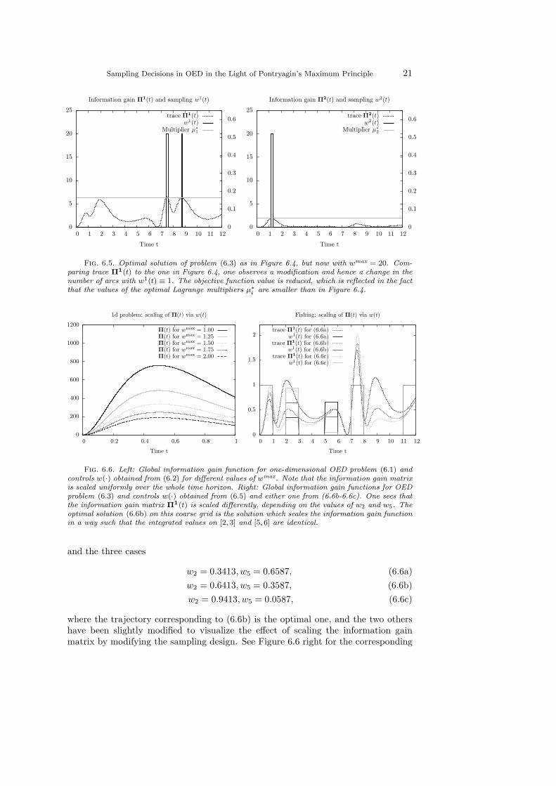
One interesting feature of one-dimensional problems is that the effect of additionalmeasurements is a pure scaling of Π(t), but not a qualitative change that would resultin measurements at different times. In other words: it is always optimal to measureas much as possible at the point / interval in time where Π(t) has its maximum value.The measurement reduces the value of Π(t), but its maximum remains in the sametime point. This is visualized in Figure 6.6 left, where the optimal sampling (6.2) fordifferent values of wmax results in differently scaled Π(t). We see in the next sectionthat this is not necessarily the case for higher-dimensional OED problems.

18 Sebastian Sager

6.2. Lotka Volterra. We are interested in estimating the parameters p2, p4 ∈ R

of the Lotka-Volterra type predator-prey fish initial value problem

x1(t) = p1 x1(t)− p2x1(t)x2(t)− p5u(t)x1(t), t ∈ [0, tf ], x1(0) = 0.5,

x2(t) = −p3 x2(t) + p4x1(t)x2(t)− p6u(t)x2(t), t ∈ [0, tf ], x2(0) = 0.7,

where u(·) is a fishing control that may or may not be fixed. The other parameters,the initial values and tf = 12 are fixed, in consistency with a benchmark problem inmixed-integer optimal control, [18]. We are interested in how to fish and when tomeasure, again with an upper bound M on the measuring time. We can measure thestates directly, h1(x(t)) = x1(t) and h

2(x(t)) = x2(t). We use two different samplingfunctions, w1(·) and w2(·) in the same experimental setting. This can be seen eitheras a two-dimensional measurement function h(x(t)), or as a special case of a multipleexperiment, in which u(·), x(·), and G(·) are identical. The experimental designproblem (3.5) then reads

minx,G,F ,z1,z2,u,w1,w2

trace(

F−1(tf))

subject tox1(t) = p1 x1(t)− p2x1(t)x2(t)− p5u(t)x1(t),x2(t) = −p3 x2(t) + p4x1(t)x2(t)− p6u(t)x2(t),˙G11(t) = fx11(·) G11(t) + fx12(·) G21(t) + fp12(·),˙G12(t) = fx11(·) G12(t) + fx12(·) G22(t),˙G21(t) = fx21(·) G11(t) + fx22(·) G21(t),˙G22(t) = fx21(·) G12(t) + fx22(·) G22(t) + fp24(·),˙F11(t) = w1(t)G11(t)

2 + w2(t)G12(t)2,

˙F12(t) = w1(t)G11(t)G12(t) + w2(t)G12(t)G22(t),˙F22(t) = w1(t)G21(t)

2 + w2(t)G22(t)2,

z1(t) = w1(t),

z2(t) = w2(t),

x(0) = (0.5, 0.7),G(0) = F (0) = 0,z1(0) = z2(0) = 0,

u(t) ∈ U , w1(t) ∈ W , w2(t) ∈ W ,0 ≤ M − z(tf)

(6.3)

with tf = 12, p1 = p2 = p3 = p4 = 1, and p5 = 0.4, p6 = 0.2 and fx11(·) =∂f1(·)/∂x1 = p1 − p2x2(t) − p5u(t), fx12(·) = −p2x1(t), fx21(·) = p4x2(t), fx22(·) =−p3+p4x1(t)−p6u(t), and fp12(·) = ∂f1(·)/∂p2 = −x1(t)x2(t), fp24(·) = ∂f2(·)/∂p4 =x1(t)x2(t).

Note that the state F21(·) = F12(·) has been left out for reasons of symmetry.We start by looking at the case where the control function u(·) is fixed to zero. Inthis case the states and the sensitivities are given as the solution of the initial valueproblem, independent of the sampling functions w1(·) and w2(·). Figure 6.2 showsthe trajectories of x(·) and G(·).

We set W = [0, 1] and M = (4, 4). The optimal solution for this control problemis plotted in Figure 6.3. It shows the sampling functions w1(·) and w2(·) and the trace


0.5

1

1.5

2

0 1 2 3 4 5 6 7 8 9 10 11 12

Time t

Differential states

Biomass Prey x1(t)Biomass Predator x2(t)

-4

-3

-2

-1

0

1

2

3

4

0 1 2 3 4 5 6 7 8 9 10 11 12

Time t

Sensitivities dx/dp

G11(t)G12(t)G21(t)G22(t)

Fig. 6.2. States and sensitivities of problem (6.3) for u(·) ≡ 0 and p2 = p4 = 1.

of the global information gain matrices

Π1(t) = F−1(tf)

(

G11(t)2 G11(t)G12(t)

G11(t)G12(t) G21(t)2

)

F−1(tf) (6.4a)

Π2(t) = F−1(tf)

(

G12(t)2 G12(t)G22(t)

G12(t)G22(t) G22(t)2

)

F−1(tf) (6.4b)

with F−1(tf) =

(

F11(tf) F12(tf)F12(tf) F22(tf)

)−1

.

0

0.2

0.4

0.6

0.8

1

1.2

0 1 2 3 4 5 6 7 8 9 10 11 120

0.002

0.004

0.006

0.008

0.01

0.012

Time t

Information gain Π1(t) and sampling w1(t)

trace Π1(t)w1(t)

Multiplier µ∗1

0

0.2

0.4

0.6

0.8

1

1.2

0 1 2 3 4 5 6 7 8 9 10 11 120

0.002

0.004

0.006

0.008

0.01

0.012

Time t


trace Π2(t)w2(t)

Multiplier µ∗2

Fig. 6.3. Optimal solution of problem (6.3) for u(·) ≡ 0 and p2 = p4 = 1. Left: measurement ofprey state h1(x(t)) = x1(t). Right: measurement of predator state h2(x(t)) = x2(t). The dotted linesshow the traces of the functions (6.4) over time, their scale is given at the right borders of the plots.One clearly sees the connection between the timing of the optimal sampling, the evolution of theglobal information gain matrix, and the Lagrange multipliers of the total measurement constraint.

Comparing this solution that measures at the time intervals when the interval overthe trace of Π(t) is maximal to a simulated one with all measurements at the firstfour time intervals, the main effect of the measurements seems to be a homogeneous

20 Sebastian Sager

downscaling over time, comparable to the one-dimensional case in the last example.The value of what could be gained by additional measurements is reduced by a factorof ≈ 10. These values for both measurement functions are, as we have seen in thelast section, identical to the Lagrange multipliers µ∗

i . The numerical result for theseLagrange multipliers are also plotted as horizontal lines in Figure 6.3. As one expectsthey are identical to the maximal values of the trace of Π(t) outside of the timeintervals in which measurements take place.

0

0.2

0.4

0.6

0.8

1

1.2

0 1 2 3 4 5 6 7 8 9 10 11 120

0.1

0.2

0.3

0.4

0.5

0.6

Time t


trace Π1(t)w1(t)

Multiplier µ∗1

0

0.2

0.4

0.6

0.8

1

1.2

0 1 2 3 4 5 6 7 8 9 10 11 120

0.1

0.2

0.3

0.4

0.5

0.6

Time t


trace Π2(t)w2(t)

Multiplier µ∗2

Fig. 6.4. Optimal solution of problem (6.3) for u(·) ≡ 0 and p2 = 1, p4 = 4. The traces ofthe information gain functions have more local maxima, hence the sampling is distributed in time.Note that the Lagrange multipliers indicate entry and exit of the functions into the intervals ofmeasurement.

The same is true for the optimal solution for problem (6.3), again with u(·) ≡ 0and M = (4, 4), but now p4 = 4. The difference in parameters results in strongeroscillations and differences between the two differential states. The optimal samplinghence needs to take the heavy oscillations into account and do measurements onmultiple intervals in time, see Figure 6.4. As one can observe, the optimal solution isa sampling design such that the values of the traces of Π(t) at the border points ofthe wi ≡ 1 arcs are identical to the values of the corresponding Lagrange multipliers.Hence, performing a measurement does have an inhomogeneous (over time) effect onthe scaling of Π(t). The coupling between measurements at different points in time,and also between different experiments, takes place via the transversality conditionsof the adjoint variables.

The inhomogeneous scaling can also be observed in Figure 6.5, where a samplingdesign for wmax = 20 is plotted. One sees that fewer measurement intervals are chosenand that the shape of the local information gain function Π1(t) is different from theone in Figure 6.4.

The same effect – an inhomogeneous scaling of the information gain function – isthe reason why fractional values w(·) 6∈ 0, 1may be obtained as optimal values whenfixed time grids are used with piecewise constant controls. We use the same scenarioas above, hence u(·) ≡ 0, M = (4, 4), and p4 = 4. Additionally we fix w2(·) ≡ 0 andconsider a piecewise constant control discretization on the grid ti = i with i = 0 . . . 12.We consider the trajectories for w1(t) = wi when t ∈ [ti, ti+1], i = 0 . . . 11 with

w0 = w7 = w11 = 1, w1 = w3 = w4 = w6 = w7 = w8 = w10 = 0 (6.5)


0

5

10

15

20

25

0 1 2 3 4 5 6 7 8 9 10 11 120

0.1

0.2

0.3

0.4

0.5

0.6

Time t


trace Π1(t)w1(t)

Multiplier µ∗1

0

5

10

15

20

25

0 1 2 3 4 5 6 7 8 9 10 11 120

0.1

0.2

0.3

0.4

0.5

0.6

Time t


trace Π2(t)w2(t)

Multiplier µ∗2

Fig. 6.5. Optimal solution of problem (6.3) as in Figure 6.4, but now with wmax = 20. Com-paring trace Π1(t) to the one in Figure 6.4, one observes a modification and hence a change in thenumber of arcs with w1(t) ≡ 1. The objective function value is reduced, which is reflected in the factthat the values of the optimal Lagrange multipliers µ∗

iare smaller than in Figure 6.4.

0

200

400

600

800

1000

1200

0 0.2 0.4 0.6 0.8 1

Time t

1d problem: scaling of Π(t) via w(t)

Π(t) for wmax = 1.00Π(t) for wmax = 1.25Π(t) for wmax = 1.50Π(t) for wmax = 1.75Π(t) for wmax = 2.00

0

0.5

1

1.5

2

0 1 2 3 4 5 6 7 8 9 10 11 12

Time t

Fishing: scaling of Π(t) via w(t)

trace Π1(t) for (6.6a)w1(t) for (6.6a)

trace Π1(t) for (6.6b)w1(t) for (6.6b)

trace Π1(t) for (6.6c)w1(t) for (6.6c)

Fig. 6.6. Left: Global information gain function for one-dimensional OED problem (6.1) andcontrols w(·) obtained from (6.2) for different values of wmax. Note that the information gain matrixis scaled uniformly over the whole time horizon. Right: Global information gain functions for OEDproblem (6.3) and controls w(·) obtained from (6.5) and either one from (6.6b-6.6c). One sees thatthe information gain matrix Π1(t) is scaled differently, depending on the values of w2 and w5. Theoptimal solution (6.6b) on this coarse grid is the solution which scales the information gain functionin a way such that the integrated values on [2, 3] and [5, 6] are identical.

and the three cases

w2 = 0.3413, w5 = 0.6587, (6.6a)

w2 = 0.6413, w5 = 0.3587, (6.6b)

w2 = 0.9413, w5 = 0.0587, (6.6c)

where the trajectory corresponding to (6.6b) is the optimal one, and the two othershave been slightly modified to visualize the effect of scaling the information gainmatrix by modifying the sampling design. See Figure 6.6 right for the corresponding

22 Sebastian Sager

information gain functions. One sees clearly the inhomogeneous scaling. The optimalsolution (6.6b) on this coarse grid is the solution which scales the information gainfunction in a way such that the integrated values on [2, 3] and [5, 6] are identical. Toget an integer feasible solution with w(·) ∈ 0, 1 we therefore recommend to refinethe measurement grid rather than rounding.

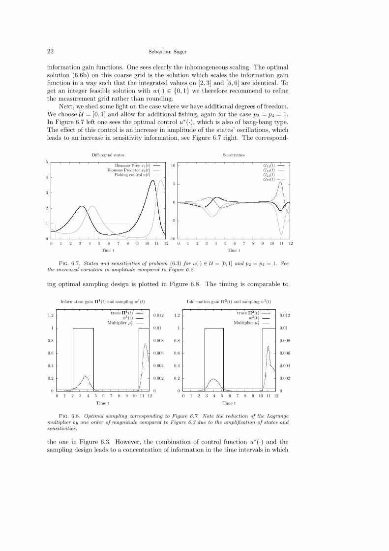
Next, we shed some light on the case where we have additional degrees of freedom.We choose U = [0, 1] and allow for additional fishing, again for the case p2 = p4 = 1.In Figure 6.7 left one sees the optimal control u∗(·), which is also of bang-bang type.The effect of this control is an increase in amplitude of the states’ oscillations, whichleads to an increase in sensitivity information, see Figure 6.7 right. The correspond-

0

1

2

3

4

5

0 1 2 3 4 5 6 7 8 9 10 11 12

Time t

Differential states

Biomass Prey x1(t)Biomass Predator x2(t)

Fishing control u(t)

-10

-5

0

5

10

0 1 2 3 4 5 6 7 8 9 10 11 12

Time t

Sensitivities

G11(t)G12(t)G21(t)G22(t)

Fig. 6.7. States and sensitivities of problem (6.3) for u(·) ∈ U = [0, 1] and p2 = p4 = 1. Seethe increased variation in amplitude compared to Figure 6.2.

ing optimal sampling design is plotted in Figure 6.8. The timing is comparable to

0

0.2

0.4

0.6

0.8

1

1.2

0 1 2 3 4 5 6 7 8 9 10 11 120

0.002

0.004

0.006

0.008

0.01

0.012

Time t


trace Π1(t)w1(t)

Multiplier µ∗1

0

0.2

0.4

0.6

0.8

1

1.2

0 1 2 3 4 5 6 7 8 9 10 11 120

0.002

0.004

0.006

0.008

0.01

0.012

Time t


trace Π2(t)w2(t)

Multiplier µ∗2

Fig. 6.8. Optimal sampling corresponding to Figure 6.7. Note the reduction of the Lagrangemultiplier by one order of magnitude compared to Figure 6.3 due to the amplification of states andsensitivities.

the one in Figure 6.3. However, the combination of control function u∗(·) and thesampling design leads to a concentration of information in the time intervals in which


measurements are being done. This is best seen by comparing the values of the La-grange multipliers in Figure 6.3 of µ∗ ≈ (1.8, 2.6)10−3 versus the ones of Figure 6.8with µ∗ ≈ (3, 3.6)10−4 which are one order of magnitude smaller.

As a last illustrating case study we consider an additional L1 penalty of thesampling design in the objective function as discussed in Section 5.2. We considerproblem (6.3) for u(·) ≡ 0 and p2 = p4 = 1 and M = ∞. The objective function nowreads

minx,G,F ,z1,z2,u,w1,w2

trace(

F−1(tf))

+

∫

T

ǫ(w1(τ) + w2(τ)) dτ (6.7)

with ǫ = 1.

0

0.2

0.4

0.6

0.8

1

1.2

0 1 2 3 4 5 6 7 8 9 10 11 12

Time t


trace Π1(t)w1(t)

Penalty ǫ

0

0.2

0.4

0.6

0.8

1

1.2

0 1 2 3 4 5 6 7 8 9 10 11 12

Time t


trace Π2(t)w2(t)

Penalty ǫ

Fig. 6.9. Optimal sampling for problem (6.3) with objective function augmented by linearpenalty term

∫Tǫ(w1(τ) + w2(τ)) dτ . The sampling functions wi(t) are at their upper bounds of 1

if and only if trace Πi(t) ≥ ǫ = 1.

As can be seen in Figure 6.9, the L1 penalization has the effect that the optimalsampling functions are given by

wi(t) =

wmax trace Πi(t) ≥ ǫ0 else

(6.8)

This implies that the value of ǫ in the problem formulation can be used to directlyinfluence the optimal sampling design. Especially for ill-posed problems with smallvalues in the information gain matrix Π(t) this penalization is beneficial from a nu-merical point of view, as it avoids flat regions in the objective function landscape thatmight lead to an increased number of iterations. Also it allows a direct economicinterpretation by coupling the costs of a single measurement to the information gain.To give an idea on the impact on the number of iterations until convergence we con-sider an instance with both measurement functions, u(·) ∈ [0, 1] and M = (6, 6).Dependent on the penalization value ǫ in (6.7) we get the following number of SQPiterations (with default settings) with the optimal control code MUSCOD-II:

ǫ 0 10−3 10−2 10−1 1 10SQP iterations 312 275 286 255 116 15

The optimal solutions are of course different, hence a comparison is somewhatarbitrary. However, it at least gives an indication of the potential.

24 Sebastian Sager

We discourage to use a L2 penalization as discussed in Section 5.3. It oftenresults in sensitivity seeking arcs with values in the interior of W , and there is nouseful economic interpretation.

7. Conclusions. We have applied the integer gap theorem and the maximumprinciple to an optimal control formulation of a generic optimum experimental designproblem. Thus we were able to analyze the role of sampling functions that determinewhen measurements should be performed to maximize the information gain with re-spect to unknown model parameters. We showed the similarity between a continuoustime formulation with measurements on intervals of time, and a formulation withmeasurements at single points in time. We defined the information gain functionsthat apply to both formulations as the result of a theoretical analysis of the necessaryconditions of optimality. Based on information gain functions we were able to shedlight on several aspects, both theoretical as by means of two numerical examples.

Differences between Fisher and Covariance Objective Function. Weshowed that the information gain matrix for a Fisher objective function has a localcharacter, whereas the one for a covariance objective function includes terms thatdepend on differential states at the end of the time horizon. This implies that mea-surements effect the information gain function in the covariance objective case, butnot in the Fisher objective case. This noncorrelation for a maximization of a functionof the Fisher information matrix has direct consequences: integral-neutral roundingof fractional solutions does not have any influence on the objective function. It alsomeans that other experiments do not influence the choice of the measurements. Third,providing a feedback law in the context of first optimize then discretize methods ispossible. All this is usually not true for Covariance Objective Functions.

Scaling of Global Information Gain Function by Measuring. Takingmeasurements changes the global information matrix Π(t). The impact may be inform of a uniform downscaling, but also as a nonhomogeneous over time modification.In the latter case it is not optimal to take as many measurements as possible in onesingle point of time, as is the case for a Fisher objective function or one-dimensionalproblems, if one allows more than one measurement per time point / interval. Thecoupling between the information function and the measurement functions takes placevia the transversality conditions, thus the impact also carries over to other experimentsand measurement functions.

Role of Lagrange multipliers. We showed that the Lagrange multipliers ofconstraints that limit the total number of measurements on the time horizon give athreshold for the information gain function. Whenever the function value is higher,measurements are performed, otherwise the value of w is 0.

Role of additional control functions. We used a numerical example to ex-amplarily demonstrate the effect of additional control functions on the shape of theinformation gain function.

Role of fixed grids and piecewise constant approximations. For the prac-tically interesting case that optimizations are performed on a given measurement gridwe showed that fractional solutions may be optimal. We recommend to further refinethe measurement grid instead of rounding.

Penalizations and ill-posed problems. By its very nature, optimal solutionsresult in small values of the global information gain function. This explains why OEDproblems are often ill-posed if the upper bounds on the total amount of measurementsare chosen too high: additional measurements only yield small contributions to theobjective function once the other measurements have been placed in an optimal way.


As a remedy to overcome this intrinsic problem of OED we propose to use L1 penal-izations of the measurement functions. We showed that the penalization parametercan be directly interpreted in terms of the information gain functions. Therefore sucha formulation would couple the costs of a measurement to a minimum amount of in-formation it has to yield, which makes sense from a practical point of view. Of course,the value of ǫ can also be decreased in a homotopy.

8. Acknowledgements. The author would like to thank the work groups ofGeorg Bock, Johannes Schloder, and Stefan Korkel for helpful and stimulating dis-cussions.

Appendix A. Useful Lemmata.In this Appendix we list several useful lemmata we use throughout the paper.Lemma A.1. (Positive trace)

If A ∈ Rn×n is positive definite, then trace(A) > 0.

Proof. As A is positive definite, it holds xTAx > 0 for all x ∈ Rn, in particular

for all unit vectors. Hence it follows aii > 0 for all i = 1 . . . n and thus triviallytrace(A) =

∑ni=1 aii > 0.

Lemma A.2. (Derivative of trace function)Let A be a quadratic n× n matrix. Then

⟨

∂trace(A)

∂A,∆A

⟩

= trace(∆A). (A.1)

Proof.⟨

∂trace(A)

∂A,∆A

⟩

= limh→0trace(A+ h∆A)− trace(A)

h

= limh→0h trace(∆A)

h= trace(∆A).

Lemma A.3. (Derivative of inverse operation)Let A ∈ GLn(R) be an invertible n× n matrix. Then

∂A−1

∂A·∆A = −A−1∆AA−1. (A.2)

Lemma A.4. (Derivative of eigenvalue operation)Let λ(A) be a single eigenvalue of the symmetric matrix A ∈ R

n×n. Let z ∈ Rn be an

eigenvector of A to λ(A) with norm 1. Then it holds⟨

∂λ(A)

∂A,∆A

⟩

= zT∆Az. (A.3)

Lemma A.5. (Derivative of determinant operation)Let A ∈ R

n×n be a symmetric, positive definite matrix. Then it holds

⟨

∂det(A)

∂A,∆A

⟩

= det(A)

n∑

i,j=1

A−1i,j ∆Ai,j . (A.4)

Proofs for the Lemmata A.3, A.4, and A.5 can be found in [9].

26 Sebastian Sager

REFERENCES

[1] A.C. Atkinson, A.N. Donev, and R.D. Tobias, Optimum experimental designs, with SAS,Oxford University Press, 2007.

[2] A. Bardow, W. Marquardt, V. Goke, H. J. Koss, and K. Lucas, Model-based measurementof diffusion using raman spectroscopy, AIChE journal, 49 (2003), pp. 323–334.

[3] I. Bauer, H.G. Bock, S. Korkel, and J.P. Schloder, Numerical methods for optimumexperimental design in DAE systems, J. Comput. Appl. Math., 120 (2000), pp. 1–15.

[4] H.G. Bock and R.W. Longman, Computation of optimal controls on disjoint control sets forminimum energy subway operation, in Proceedings of the American Astronomical Society.Symposium on Engineering Science and Mechanics, Taiwan, 1982.

[5] A.E. Bryson and Y.-C. Ho, Applied Optimal Control, Wiley, New York, 1975.[6] G. Franceschini and S. Macchietto, Model-based design of experiments for parameter pre-

cision: State of the art, Chemical Engineering Science, 63 (2008), pp. 4846–4872.[7] D. Janka, Optimum experimental design and multiple shooting, master’s thesis, Universitat

Heidelberg, 2010.[8] H.J. Kelley, R.E. Kopp, and H.G. Moyer, Singular extremals, in Topics in Optimization,

G. Leitmann, ed., Academic Press, 1967, pp. 63–101.[9] S. Korkel, Numerische Methoden fur Optimale Versuchsplanungsprobleme bei nichtlinearen

DAE-Modellen, PhD thesis, Universitat Heidelberg, Heidelberg, 2002.[10] S. Korkel and E. Kostina, Numerical methods for nonlinear experimental design, in Mod-

elling, Simulation and Optimization of Complex Processes, Proceedings of the InternationalConference on High Performance Scientific Computing, Hans Georg Bock, E. Kostina, H. X.Phu, and R. Rannacher, eds., Hanoi, Vietnam, 2004, Springer, pp. 255–272.

[11] S. Korkel, E. Kostina, H.G. Bock, and J.P. Schloder, Numerical methods for optimalcontrol problems in design of robust optimal experiments for nonlinear dynamic processes,Optimization Methods and Software, 19 (2004), pp. 327–338.

[12] S. Korkel, A. Potschka, H.G. Bock, and S. Sager, A multiple shooting formulation foroptimum experimental design, Mathematical Programming, (2012). (submitted).

[13] S. Korkel, H. Qu, G. Rucker, and S. Sager, Derivative based vs. derivative free optimiza-tion methods for nonlinear optimum experimental design, in Proceedings of HPCA2004Conference, August 8-10, 2004, Shanghai, 2005, Springer, pp. 339–345.

[14] H.J. Pesch and R. Bulirsch, The maximum principle, Bellman’s equation and Caratheodory’swork, Journal of Optimization Theory and Applications, 80 (1994), pp. 203–229.

[15] L.S. Pontryagin, V.G. Boltyanski, R.V. Gamkrelidze, and E.F. Miscenko, The Mathe-matical Theory of Optimal Processes, Wiley, Chichester, 1962.

[16] F. Pukelsheim, Optimal Design of Experiments, Classics in Applied Mathematics 50, SIAM,2006. ISBN 978-0-898716-04-7.

[17] S. Sager, H.G. Bock, and M. Diehl, The integer approximation error in mixed-integer op-timal control, Mathematical Programming, (2011). (accepted).

[18] S. Sager, H.G. Bock, M. Diehl, G. Reinelt, and J.P. Schloder, Numerical methods foroptimal control with binary control functions applied to a Lotka-Volterra type fishing prob-lem, in Recent Advances in Optimization, A. Seeger, ed., vol. 563 of Lectures Notes inEconomics and Mathematical Systems, Heidelberg, 2006, Springer, pp. 269–289. ISBN978-3-5402-8257-0.

[19] S. Sager, G. Reinelt, and H.G. Bock, Direct methods with maximal lower bound for mixed-integer optimal control problems, Mathematical Programming, 118 (2009), pp. 109–149.

[20] K. Schittkowski, Experimental design tools for ordinary and algebraic differential equations,Mathematics and Computers in Simulation, 79 (2007), pp. 521–538.

[21] J. Schoneberger, H. Arellano-Garcia, H. Thielert, S. Korkel, and G. Wozny, Opti-mal experimental design of a catalytic fixed bed reactor, in Proceedings of 18th EuropeanSymposium on Computer Aided Process Engineering - ESCAPE 18, B. Braunschweig andX. Joulia, eds., 2008.

[22] S.P. Sethi and G.L. Thompson, Optimal Control Theory: Applications to Management Sci-ence and Economics, Springer, 2nd edition ed., 2005. ISBN-13: 978-0387280929.

Documents

SAMPLING DECISIONS IN OPTIMUM EXPERIMENTAL DESIGN IN …