Embed Size (px)
Citation preview

Sampling and Consideration of
Variability (Temporal and Spatial) For Monitoring of
Recreational Waters
U.S. Environmental Protection Agency Office of Water
EPA-823-R-10-005
December 2010

This page is intentionally blank.

U.S. Environmental Protection Agency—Office of Water
December 2010 i
Contents Executive Summary .................................................................................................................................... 1 CHAPTER 1 Introduction and Background ............................................................................................ 5
1.1. Purpose .......................................................................................................................................... 5 1.2. EPA Monitoring Research for New or Revised Recreational Water Quality Criteria .................. 5 1.3. Summary of Previous EPA Recommended Water Quality Criteria ............................................. 5
1.3.1. Previous EPA Recreational Ambient Water Quality Criteria ............................................... 6 1.3.2. Current EPA Recreational AWQC........................................................................................ 6 1.3.3. EPA National BEACH Guidance and Required Performance Criteria for Grants ............... 6
1.4. Organization of this Report ........................................................................................................... 7 CHAPTER 2 Findings on Indicator Density and Temporal Variability ............................................... 9
2.1. Variability with Time Scales Less than 1 Hour .......................................................................... 10 2.1.1. Coastal Sites ........................................................................................................................ 10 2.1.2. River and Stream Sites ........................................................................................................ 10 2.1.3. Summary ............................................................................................................................. 11
2.2. Diurnal Variations ....................................................................................................................... 11 2.2.1. Coastal Sites ........................................................................................................................ 12 2.2.2. River and Stream Sites ........................................................................................................ 13 2.2.3. Summary ............................................................................................................................. 13
2.3. Variations Related to Tidal Processes ......................................................................................... 13 2.4. Variability Attributable to Rainfall and Runoff (Event-Scale Variability) ................................. 15
2.4.1. River and Stream Sites ........................................................................................................ 15 2.4.2. Coastal Sites ........................................................................................................................ 16 2.4.3. Summary ............................................................................................................................. 17
2.5. Monthly and Seasonal Variability ............................................................................................... 18 2.5.1. River and Stream Sites ........................................................................................................ 18 2.5.2. Coastal Sites ........................................................................................................................ 20 2.5.3. Summary ............................................................................................................................. 20
2.6. Predictive Power of Prior Day’s Indicator Density ..................................................................... 21 CHAPTER 3 Findings on Indicator Density and Spatial Variability .................................................. 23
3.1. Indicator Density Variation with Water Depth at the Point of Sample Collection ..................... 25 3.1.1. Coastal Sites ........................................................................................................................ 25 3.1.2. River and Stream Sites ........................................................................................................ 28 3.1.3. Summary ............................................................................................................................. 28
3.2. Indicator Density Variation with Depth Below Surface of Sample Collection .......................... 30 3.2.1. Inland Sites .......................................................................................................................... 30 3.2.2. Coastal Sites ........................................................................................................................ 31 3.2.3. Summary ............................................................................................................................. 31
3.3. Along-Shore Spatial Variability .................................................................................................. 31 3.4. Longitudinal Spatial Variation, Streams and Lakes .................................................................... 36 3.5. Cross-Sectional Variations in Indicator Densities in Streams .................................................... 38 3.6. Beach Features Promoting Non-Homogeneity in Indicator Density .......................................... 39 3.7. Inferences from Single and Composite Samples ........................................................................ 40
CHAPTER 4 Development of Monitoring Approach ............................................................................ 43 4.1. Factors to Consider for Monitoring Plan Development .............................................................. 43 4.2. Site Characterization ................................................................................................................... 43
4.2.1. Sanitary Surveys ................................................................................................................. 43

U.S. Environmental Protection Agency—Office of Water
December 2010 ii
4.2.2. Pilot Studies ........................................................................................................................ 44 4.3. Monitoring Approaches and Statistics for Assessing Water Quality .......................................... 46
4.3.1. Statistical Considerations: Variability, Confidence Estimates, and Sample Numbers ....... 47 4.3.2. Statistical Considerations for Spatial Sampling. ................................................................. 48 4.3.3. Statistical Considerations for Temporal Sampling. ............................................................ 49
4.4. Summary of Monitoring Approaches and Considerations .......................................................... 50 4.4.1. Review of Indicator Density Variability ............................................................................. 50 4.4.2. Where to Sample ................................................................................................................. 51 4.4.3. When to Sample .................................................................................................................. 52 4.4.4. How to Sample .................................................................................................................... 53 4.4.5. How Often to Sample .......................................................................................................... 53
CHAPTER 5 References........................................................................................................................... 55
Tables Table 1. Summary statistics for distribution of E. coli density over 24 hours for three streams ................ 11 Table 2. Fraction of exceedances missed for different sampling schemes ................................................. 21
Figures Figure 1. Distribution of indicator sources in a coastal setting near a point source. ................................... 23 Figure 2. Transport processes in the surf zone (plan view). ....................................................................... 24 Figure 3. Indicator density variation with water depth at sample collection, 9:00 a.m. samples,
EMPACT Study (E. coli for West Beach and Belle Isle and Enterococcus for other beaches) ....................................................................................................................................... 27
Figure 4. Indicator density variation with water depth at sample collection, 2:00 p.m. samples, EMPACT Study (E. coli for West Beach and Belle Isle and Enterococcus for other beaches) ....................................................................................................................................... 27
Figure 5. Dispersion, advection, and removal in the surf zone ................................................................... 32 Figure 6. Variation in fecal coliform density downstream of a sewage outfall. ......................................... 37 Figure 7. E. coli density along cross-stream transects of the Charles River. .............................................. 39 Figure 8. Illustration of beach features promoting non-uniform indicator density in parts of a beach. ...... 40 Figure 9. Illustration of uneven fecal pollution loading and potential sample locations. ........................... 45 Figure 10. Illustration of beach features interfering with mixing. .............................................................. 45 Figure 11. Confidence intervals tighten with increasing number of samples. ............................................ 47

U.S. Environmental Protection Agency—Office of Water
December 2010 iii
Abbreviations and Acronyms AFRI acute febrile respiratory illness ANN artificial neural network (model) ANOVA analysis of variance AWQC ambient water quality criteria BEACH Act Beaches Environmental Assessment and Coastal Health Act CAFO concentrated animal feeding operation CFU colony forming unit CL confidence limit CPSP Critical Path Science Plan CSO combined sewer overflow CV coefficient of variation CWA Clean Water Act DGD discrete growth distribution DPLSR dynamic partial least-squares regression (model) EMC event mean concentration EMPACT Environmental Monitoring for Public Access and Community Tracking EPA U.S. Environmental Protection Agency EU European Union FIB fecal indicator bacteria GI gastrointestinal HCGI highly credible gastrointestinal illness LOAEL lowest observed adverse effect level MF membrane filtration MPN most probable number MS4 municipal separate storm sewer system MSE mean sum of errors MTF multiple tube fermentation NEEAR National Epidemiological and Environmental Assessment of Recreational NOAEL no-observed-adverse-effect level NPDES National Pollutant Discharge Elimination System NPS nonpoint source (pollution) NRC National Research Council OLSR ordinary least squares regression (model) ORP oxidation reduction potential PC prospective cohort PCR polymerase chain reaction POTW publicly owned (sewage/wastewater) treatment works

U.S. Environmental Protection Agency—Office of Water
December 2010 iv
qPCR quantitative polymerase chain reaction QPCRCE qPCR cell equivalents RMSE root mean square error ROC receiver operating characteristic (analysis) SSM single sample maximum SSO sanitary sewer overflow TMA transcription-mediated amplification TMDL total maximum daily load U.K. United Kingdom WHO World Health Organization (United Nations) WQS water quality standard[s] WWTP wastewater treatment plant

U.S. Environmental Protection Agency—Office of Water
December 2010 1
Executive Summary This report reviews the literature on temporal and spatial variability of fecal indicator organism density at recreational sites and the implications of variability for the design of sampling plans. For all sites, the greatest temporal variability in indicator densities is from rain events. For coastal water quality sampling locations, the greatest spatial variabilities are those related to sample depth and site features, such as the alignment of fecal pollution sources with a beach. For inland recreational sites, along-stream variability is most important. For coastal sites, pilot monitoring and sanitary surveys are useful tools for collecting site information. These should be performed before development of monitoring plans and sampling microbial water quality in the morning, at waist depth, and at multiple locations selected according to the site characteristics. For inland sites, sample locations can be selected on the basis of known or suspected locations of fecal pollution sources and the locations where recreational activity is likely.
Methodology A literature review was performed to identify and compile the information used to develop this report. The review included specific searches for information on physical and biological processes at temporal and spatial scales relevant to indicator organism variability for coastal and inland waters. On the basis of the results of the review, the report summarizes key findings to help in the design of appropriate recreational water quality sampling schemes that are protective of human health.
This report emphasizes research and findings primarily from studies using culture-based methods. Non-culture-based methods (e.g., quantitative polymerase chain reaction) are mentioned and discussed where information is available. Such information, however, is not well described in the literature. Accordingly, this report acknowledges the expected future importance and relevance of non-culture-based methods for developing and implementing EPA’s new or revised recreational water quality criteria. In addition, the attributes of current fecal indicators and available enumeration methods, along with their inherent uncertainties, are not discussed in this report, despite their importance in interpreting monitoring results.
Summary of Key Findings The literature review revealed that several factors influence temporal and spatial variability of fecal indicators in recreational waters, although with different degrees of importance. The ranking of those factors is illustrated in Exhibit 1. Discrete events (e.g., precipitation events or combined sewer overflow [CSO] discharges) have by far the greatest impact on temporal variability, while sample depth and along-stream sampling have the greatest impact on spatial variability for coastal and inland sites, respectively. Most important, specific knowledge of a recreational site is crucial, and appropriate site investigation is paramount to achieving an accurate and comprehensive understanding of the factors influencing fecal pollution and associated risks to human health at that site.

U.S. Environmental Protection Agency—Office of Water
December 2010 2
Temporal variability This report points to the global importance of climatic features (e.g., temperature, storm events, day/night duration, tide intensity) on indicator variability along with the indirect consequences on loading through increased recreational activities and associated risks in warmer seasons and locales. The importance of human-made events (e.g., treated wastewater effluent discharges) is also highlighted.
Spatial variability: coastal sites The sample depth, related to the swimmer’s distance from the shoreline (e.g., ankle- and waist-depth) exhibits higher spatial variability than along-shore variations or variations with depth at which a sample is drawn. Site features that either promote or prevent mixing can have a strong influence on the distribution of indicators along a coastline. The impact of site features highlights the importance of sanitary surveys in developing monitoring schemes.
Spatial variability: inland sites Variability along (longitudinally) streams and estuaries is generally greater than that associated with vertical depth of sampling from the water surface or cross-stream variability. As with coastal sites, this finding emphasizes the importance of identifying fecal pollution sources through a sanitary survey before developing water quality monitoring plans.
Statistical assessment of water quality Along-shore variation of indicator density at coastal sites appears best characterized by a lognormal distribution. When interpreting the results of multiple samples taken at a site, the geometric mean of indicator densities is considered the best metric for characterizing water quality, because the geometric has been demonstrated to correlate with incidence of illness in epidemiological studies conducted at coastal sites. In general, for large sites requiring multiple samples to characterize water quality, discrete sampling at multiple points is suggested; although, using composite sampling could provide a valuable tradeoff between cost and effort and precision for assessing fecal indicator densities.
Exhibit 1. Ranking of factors influencing variability of fecal indicators in natural systems
Note: Temporal variability at a short time scale is ranked lowest, except for samples obtained at ankle depth and shallower.

U.S. Environmental Protection Agency—Office of Water
December 2010 3
Monitoring Considerations All the above factors influencing the variability of fecal indicator densities need to be taken into account when designing a monitoring scheme for a specific recreational site. On the basis of the factors illustrated in Exhibit 1 and specific features at a site, the following approach can be used to help design a monitoring plan (Exhibit 2). Pilot monitoring studies and sanitary surveys are the best tools available for collecting data required to develop effective site-specific monitoring plans.
Exhibit 2. Monitoring considerations for recreational waters
HOW Multiple approaches for choice of location and number of samples, based on site specific constraints and historical data:
Power-curve approach sampling based on
site-specific variance Limited sampling based on constraints
Composite sampling
WHEN Morning samples yield conservative results relating water quality to human health effects when using culture methods, whereas the use of qPCR methods yields results that are relatively stable throughout the day. Sample collection frequency could be related to site charac-terization, site usage, or practical constraints.
WHERE Area allowing best and most efficient characterization:
Link to fecal pollution No native sources Small variability
Coastal
Knee-deep or greater Knowledge of
hydrodynamics
Inland
Knowledge of stream Top 6 inches of water
column

U.S. Environmental Protection Agency—Office of Water
December 2010 4
This page is intentionally blank.

U.S. Environmental Protection Agency—Office of Water
December 2010 5
CHAPTER 1 Introduction and Background 1.1. PURPOSE The purpose of this document is to meet one of the elements (Project P-12) in the U.S. Environmental Protection Agency’s (EPA’s) Critical Path Science Plan for Development of New or Revised Recreational Water Quality Criteria (CPSP) (USEPA 2007a).1 The intent of Project P-12 is to provide detailed reference information so that EPA can “design and evaluate a monitoring approach that will characterize the quality of beach waters that takes into account the spatial and temporal variability associated with water sampling.” After publication of its new or revised recreation water quality criteria, EPA expects to use information from this report and other materials to develop implementation recommendations.
1.2. EPA MONITORING RESEARCH FOR NEW OR REVISED RECREATIONAL WATER QUALITY CRITERIA
In 2002 EPA published Environmental Monitoring for Public Access and Community Tracking (EMPACT) Beaches Project: Time-Relevant Beach and Recreational Water Quality Monitoring and Reporting (USEPA 2002a) and in 2005 the EMPACT Beaches Project: Results from a Study on Microbiological Monitoring in Recreational Waters (USEPA 2005). Both of those projects were part of the EMPACT Program. Given its obvious relevance to this report, data from the EMPACT Program is discussed and analyzed in Chapter 4 of this report.
EPA has also been conducting the National Epidemiological and Environmental Assessment of Recreational (NEEAR) Water Study,2 which is a series of prospective cohort (PC) epidemiological studies beginning in 2002 at several Great Lakes (freshwater) recreational beaches and continuing at marine beaches. The purpose of the NEEAR epidemiology studies is to determine the association of swimming illness with fecal indicator levels in recreational waters.
1.3. SUMMARY OF PREVIOUS EPA RECOMMENDED WATER QUALITY CRITERIA
A brief review of the microbiological guidelines and standards/criteria for recreational waters and their context for development and implementation, as addressed by the EPA, is presented below.
1 Report is at http://www.epa.gov/waterscience/criteria/recreation/plan/index.html. 2 Further information about the NEEAR Water Study is at http://www.epa.gov/nheerl/neear/index.html.

U.S. Environmental Protection Agency—Office of Water
December 2010 6
1.3.1. PREVIOUS EPA RECREATIONAL AMBIENT WATER QUALITY CRITERIA The ambient water quality criteria (AWQC) for the United States that were proposed in 1968 and recommended again in 1976 were established on the basis of the epidemiological studies conducted during the late 1940s and early 1950s by the U.S. Public Health Service (Stevenson 1953). Those criteria for recreational waters were, “As determined by multiple-tube fermentation or membrane filter procedures and based on a minimum of not less than five samples taken over not more than a 30-day period, the fecal coliform content of primary contact recreation waters shall not exceed a log mean of 200/100 millilters [mL], nor shall more than 10 percent of total samples during any 30-day period exceed 400/100 mL.”
1.3.2. CURRENT EPA RECREATIONAL AWQC EPA’s current water quality criteria for recreational exposure to surface waters (USEPA 1986) are based on the observed occurrence of gastrointestinal (GI) illness associated with swimming in fresh (USEPA 1984) or marine (USEPA 1983) recreational waters as determined through several PC epidemiology studies conducted in the 1970s and early 1980s.
For marine recreational waters, based on a statistically significant number of samples (generally not less than five samples equally spaced over a 30-day period), a steady state (i.e., dry weather conditions) geometric mean indicator density of 35 CFU (colony forming units)/100 mL of enterococci was recommended; for fresh recreational waters, a steady state geometric mean indicator density of 33 CFU/100 mL for enterococci or 126 CFU/mL for Escherichia coli was recommended. In addition, no single sample should exceed a one-sided confidence limit (CL) value calculated for each indicator according to four different levels of beach usage (i.e., established single sample maximums [SSMs]). In this regard, the 1986 bacteria criteria recommended different SSMs depending on beach usage levels. The levels correspond to the following four SSMs: designated bathing beach for the 75 percent (most protective) CL, moderate use for bathing for the 82% CL, light use for bathing for the 90 percent CL, and infrequent use for bathing for the 95 percent CL. Thus, where a given recreational area has a greater potential for more people to be exposed, a higher degree of protectiveness (i.e., a lower SSM) was recommended.
Those recommended criteria are in effect and required for use at coastal and Great Lakes waters designated for swimming or similar water contact activities, except where the state or territory has in place EPA-approved criteria that are as protective of human health as EPA’s 1986 recommendations (USEPA 2004). EPA also published a fact sheet (USEPA 2006a) that addresses questions regarding the appropriate risk level (or levels) a state may choose when adopting into the state’s water quality standards (WQS) bacteria criteria to protect its coastal recreation waters. Another fact sheet (USEPA 2006b) addresses the appropriate use of the SSM values component of EPA’s 1986 bacteria criteria in coastal recreation waters.
1.3.3. EPA NATIONAL BEACH GUIDANCE AND REQUIRED PERFORMANCE CRITERIA FOR GRANTS
EPA’s National Beach Guidance and Required Performance Criteria for Grants (USEPA 2002b) provides performance criteria for monitoring and assessment of coastal recreation waters

U.S. Environmental Protection Agency—Office of Water
December 2010 7
adjacent to beaches, and for prompt public notification of any exceedance or likelihood of exceedance of applicable WQS for pathogens and pathogen indicators for coastal recreation waters. It also outlines the eligibility requirements for monitoring and notification program implementation grants under CWA section 406(b).
That beach guidance document provides EPA’s current requirements and recommendations for monitoring beach waters. Chapter 3 of that guidance establishes procedures for states to evaluate and rank their beaches according to risk or usage (or both) and establish a priority tiering system. Chapter 4 of that document requires that states develop a Tiered Monitoring Plan, consistent with the priority ranking of their beaches. Requirements and recommendations are included for a variety of monitoring circumstances and other monitoring/assessment issues. For each of the tiers, it offers recommendations such as when to conduct basic sampling; when to conduct additional sampling; where to collect samples; what depth to collect samples, and such. More detailed monitoring considerations are discussed in Appendix H of the document. Chapter 5 of that document sets forth the public notification requirements and recommendations for a tiered notification system.
1.4. ORGANIZATION OF THIS REPORT To prepare this report, a detailed literature search and retrieval was conducted. Chapter 2 provides findings from the literature on temporal variability of indicator density for all relevant time scales. Chapter 3 provides findings from the literature on spatial variability of indicator density at all relevant length scales and directions. Chapter 4 draws and builds on Chapters 2 and 3 to describe when, where, and how monitoring could be conducted such that it is consistent with and accounts for the spatial and temporal variability inherent in fecal indicator organism densities in natural systems. Last, on the basis of findings from the literature and analyses, Chapter 4 also lays out factors to consider in determining where to sample, when to sample, and how to sample for recreational microbial water quality purposes.
It is important to note that culture-derived quantification methods (e.g., membrane filtration, Enterolert® and Colilert®) are the only EPA-approved methods for regulatory monitoring of fecal indicators. Therefore, the majority of the phenomena described in this report relate indicator variability (temporal and spatial) for indicator densities enumerated via culture methods. It is not suggested that variability will be the same when different methods are used, only that the body of literature available for assessing variability for culture-independent methods is relatively small. Particularly in the case of the quantitative polymerase chain reaction assay (qPCR), the variability of the indicator signal in both space and time can differ from that of the culture signal. The persistence of genetic material differs from that of live, viable cells; the uncertainty of molecular methods could be significantly different from that of culture methods. However, in the past decade, culture-independent enumeration methods (e.g., qPCR) have grown widely in use and sophistication and are likely to become standardized as a regulatory monitoring tool, mainly thanks to their rapidity and ability to enumerate non-culturable organisms. Thus, relevant information related to such methods is cited where appropriate in this report. As discussed in Section 4.8, work is under way to assess the inherent variability of the methods for use as a monitoring tool for recreational waters.

U.S. Environmental Protection Agency—Office of Water
December 2010 8
This page is intentionally blank.

U.S. Environmental Protection Agency—Office of Water
December 2010 9
CHAPTER 2 Findings on Indicator Density and Temporal Variability
This chapter discusses the temporal variability of indicator organism density. The phenomena described in this chapter and Chapter 3 form the basis for considerations and suggestions in Chapter 4 about where, when, and how recreational water quality sampling should be conducted. More specifically, this section presents findings from a literature review of published studies on the temporal variability of indicator density for relevant time scales, sorted by waterbody type (coastal versus inland rivers and streams).
Temporal variability in indicator density—at time scales ranging from minutes to months—has been observed in time series analyses of indicator density. Variations with time scales on the order of minutes are important because such considerations influence the number of samples needed to accurately characterize microbial water quality and the confidence with which to ascribe results of sampling events. Variations with times scales on the order of tens of minutes are important because they have the same time scale as that of typical recreational use episodes. Variations with time scales on the order of a day are important because their knowledge allows comparison between samples taken at different times of the day or between samples taken on successive days.
The tradeoff between sampling cost and effort and protection of public health is illustrated by Fleisher (1985, 1990). In those two studies, reanalysis of total coliform data collected over a 3-year period shows that variability in indicator density resulted in potential mis-classification of water quality for 33 percent, 64 percent, and 71 percent of sampling dates for the first, second, and third years of the study, respectively. Reanalysis entailed classifying sample results as above or below the criterion on the basis of their 95 percent confidence interval, rather than a simple arithmetic mean or geometric mean of samples taken over a given period (for more discussion of arithmetic mean versus geometric mean, see Section 4.1.1). The authors also found that contradictory water quality determinations could often be made on the basis of morning and afternoon sample results. Method uncertainty and temporal variability both contributed to the overall uncertainty in water quality. The observations led Fleisher (1990) to recommend replicate samples be drawn at bathing sites and that replicate laboratory analyses be performed on sample splits.
The use of lognormal distribution for describing the distribution of indicator densities at a site or between sites is described in greater detail in sections that follow, and thus is only briefly discussed below. In general, time series non-log-transformed indicator data are characterized by long tails at high indicator organism densities. The long tails result from the very high indicator densities associated with rain events and the frequency with which such events occur. Thus, the temporal distribution of indicators at a coastal site is often assumed well characterized by a lognormal distribution. For example, results from enumeration of enterococci in 11,000 bathing water samples collected from marine sites in the U.K. were fit with a lognormal distribution with a mean of 0.9337 (i.e., a geometric mean of 9 enterococci/100 mL), standard deviation of 0.8103 and a 95th percentile value of 2.267 (i.e., 185 enterococci/100 mL) (Kay et al. 2004). Kim and Grant (2004) also found that a lognormal distribution provided a good fit to a relatively large

U.S. Environmental Protection Agency—Office of Water
December 2010 10
(n = 860) data set of enterococci observations (goodness of fit was assessed via a Kolmogorov-Smirnov test for normality); however, the distribution mean and standard deviation were not reported.
2.1. VARIABILITY WITH TIME SCALES LESS THAN 1 HOUR
2.1.1. COASTAL SITES At two marine beaches, Boehm (2007) noted very high variability in enterococci density at time scales less than 1 hour. The high short-time-scale temporal variability was determined to not be the result of method uncertainty (the Enterolert® most probable number (MPN) method was used for bacteria enumeration in that study) and was not random (white noise). Rather, enterococci time series were found to be fractal, with variability in densities related to physical and biological processes occurring at the sample locations. For samples drawn at 10-minute intervals, average variability (as change in concentration between consecutive samples) was 60 percent and as high as 700 percent. To achieve a coefficient of variation of 50 percent around the one-hour mean, the number of samples at the four sampling points (on two beaches) evaluated in the study was estimated to be 6, 5, 4, and 4, respectively. To achieve a 20 percent coefficient of variation, the number of samples was estimated to be 39, 31, 25, and 25 for the four sampling locations.
For samples taken at 1-minute intervals at a single sample location (samples taken at ankle depth on incoming waves and analyzed via Enterolert®, with results reported as MPN/100 mL), Boehm (2007) again observed high variability, with an average enterococci density change between consecutive samples of 34 MPN/100 mL/minute and a maximum change of 140 MPN/100 mL/minute. To achieve coefficients of variation of 20 percent and 50 percent relative to the 10-minute mean enterococci density, 10 and 2 samples would have to be drawn, respectively.
In an earlier study of short time-scale temporal variation in indicator density, Boehm et al. (2002) noted high variability between samples taken at 10-minute intervals. Samples in that study were collected at ankle depth for incoming waves. Many observances of samples significantly below WQS followed by samples significantly exceeding the same WQS were reported. Transport of pulses of enterococci via rip currents (time scale on the order of hours) was inferred from observation of elevated enterococci densities at five locations along the beach. The authors estimated that, for the water quality monitored during the studies, 70 percent of single sample exceedances (104 MPN/100 mL) have durations of less than 1 hour, and 40 percent have durations of less than 10 minutes.
2.1.2. RIVER AND STREAM SITES Variability over short time scales has been observed at inland streams and at coastal sites. Meays et al. (2006) studied E. coli variability in three streams—two in areas dominated by agricultural and forested land use and one downstream of an area of recreational use. The mean, minimum, maximum and standard deviation of E. coli density (data not log-transformed) for samples drawn at 15-minute intervals for 24-hour monitoring are presented in Table 1. Both between-sample and longer time scale variabilities were observed in E. coli densities. A period of elevated E. coli

U.S. Environmental Protection Agency—Office of Water
December 2010 11
density was observed during the afternoon hours at the site with the highest mean E. coli density, which was attributed to a rainfall event that occurred on the morning of the study.
Table 1. Summary statistics for distribution of E. coli density over 24 hours for three streams
Creek Mean Minimum Maximum Standard deviation
Duteau Creek (primarily agricultural and forest land use)
4 0 13 2.3
Deer Creek (primarily agricultural and forest land use)
19 6 79 11.8
BX Creek (downstream from a recreation area)
156 22 696 181.4
Source: Meays et al. 2006
Because variability differs between streams and arises from a complex set of factors, the authors recommend that an understanding of the sources for a site (e.g., by executing a sanitary survey) be developed before designing and implementing monitoring programs.
2.1.3. SUMMARY Significant short time-scale variability has been observed at shallow (ankle-depth) coastal sites (Boehm 2007). Extreme variability in indicator density is generally limited to shallow sites and is likely related to mobilization of sediment-associated indicator bacteria by wave action. Short-term variability is less pronounced at locations with greater water depth. Two strategies for overcoming short time-scale variability when assessing bacteriological water quality are to select sample sites with less variability (e.g., sites at greater water depth) or to use composite samples if sampling at locations with high variability cannot be avoided or is required.
Short-term variability (time scales of less than 1 hour) has also been observed in streams. Event-scale and diurnal variability are generally greater than short-term variability in streams; although, sudden loading can result in rapid changes in stream indicator density. Because short time-scale variability in streams is less significant than other variabilities, short time-scale fluctuations are not a significant factor in developing sampling plans for stream sites.
2.2. DIURNAL VARIATIONS Several studies have identified diurnal variation in indicator density in marine and freshwater coastal environments, streams, and non-flowing inland waters (e.g., Brenniman et al. 1981; Boehm et al. 2002; Whitman et al. 2004a; Whitman and Nevers 2004b; Noble et al. 2005; Liu et al. 2006; Meays et al. 2006; Rosenfeld et al. 2006; Traister and Anisfeld 2006; He et al. 2007). All other factors being equal, when measured by culture methods, fecal indicator bacteria demonstrate a predictable pattern of highest density in the morning, decreasing density during the day (often by several orders of magnitude), reaching the lowest density in the mid-afternoon, and followed by a sharp rebound of density in the late evening. The decrease of indicator bacteria during daylight hours results from inactivation of organisms by incident solar radiation (Sinton et al. 2002) and

U.S. Environmental Protection Agency—Office of Water
December 2010 12
possibly from increased removal of organisms via predation (Menon et al. 2003; Boehm et al. 2005a). The rapid rebound of indicator density during evening hours remains incompletely understood (Boehm 2007). Although the likely cause of rapid rebound is resuscitation of viable but non-culturable cells, it is possible that other processes such as replenishment of viable indicators from other sources (sediments, influent waters) also play a role.
In contrast to indicator diurnal variation by culture methods, indicator density diurnal variation for qPCR methods is lower, with relatively stable indicator density reported for samples taken throughout the day (e.g., as observed at Great Lakes beaches by Wade et al. 2006). This is apparently due to the different persistence and sensitivity to light molecular material versus viable culture cells. Those differences result in differences in diurnal variation in indicator densities when measured by the two techniques. In studies of light and dark marine water mesocosms, Walters et al. (2009) found that decay rates of naked genetic material were the same in both types of mesocosms, whereas inactivation of culturable cells was faster in light mesocosms than dark ones. Further, the persistence of naked genetic material was significantly longer than that of intact viable cells in marine water and in sewage. The findings suggest that variability of indicators as measured by qPCR is likely different from that of indicators as measured by culture-based methods. That difference is expected to be pronounced for diurnal variability of indicator densities in streams, inland lakes, and coastal sites.
2.2.1. COASTAL SITES In a comparison of fecal coliform, total coliform, and enterococci survival in marine environments and mesocosms, Boehm et al. (2002) found that mesocosm indicator organism densities declined when mesocosms were exposed to natural sunlight, but they did not rebound during evening and nighttime hours. In contrast, bacteria populations in the surf zone exposed to the same solar radiation rebounded rapidly, reaching morning density levels by approximately 8:00 in the evening. Reasons for differences between mesocosm and in situ populations include rapid replenishment of bacteria from sediments or other sources, or growth outpacing inactivation/removal in situ during periods of low solar radiation intensity. In general, because of the predictable variation in microbiological water quality during the course of a day, morning water quality assessments are good predictors of afternoon water quality determinations. For example, in a study of marine beaches, Corbett et al. (1993) found that a strong correlation existed between passing water quality determination (in this case, geometric mean fecal coliform count less than 300/100 mL) in a morning test and subsequent pass in an afternoon test, while there was a 50 percent chance of water quality failing the afternoon test on days when the morning test resulted in a failure.
However, in support for EPA epidemiological studies conducted at inland (Great Lakes) bathing beaches, Haugland et al. (2005) and Wade et al. (2008) observed that, in contrast to culture-based method results, qPCR counts of enterococci in Great Lakes waters were relatively constant during the day, which is consistent with the explanation provided at the end of Section 1.3.

U.S. Environmental Protection Agency—Office of Water
December 2010 13
2.2.2. RIVER AND STREAM SITES Traister and Anisfeld (2006) observed diurnal variation of E. coli in five temperate streams except on days in which loads of E. coli from rainfall/runoff masked the die-off of bacteria in the afternoon. The daily fluctuations in E. coli density on streams were found to be more pronounced on slower-flowing, less shaded stream reaches than on smaller, more shaded ones. Meays et al. (2006) observed that stream indicator density response to rainfall was much greater than diurnal variability due to UV radiation or temperature effects and die-off.
A potential anthropogenic cause for diurnal indicator density fluctuations is the variable loading of surface waters of raw (untreated) and treated sewage. Bordalo (2003) observed that fecal coliform density in raw sewage discharged to a river 3.3 kilometers (km) upstream of its mouth exhibited high temporal variability, reaching a peak concentration around 1012 CFU/100 mL around 9:00 a.m., a second, less distinguishable peak around 108 CFU/100 mL around 8:00 p.m., and a low value of less than 10 CFU/100 mL at 10:00 p.m. Indicator density and loadings for treated sewage are also expected to vary with time of day, although not as radically as for raw sewage.
2.2.3. SUMMARY Regardless of the cause of diurnal fluctuations in indicator density as measured using culture-based methods, the universal observance of the fluctuations dictates that sampling should be conducted at the same time each day if water quality is to be compared between days and that sampling in the morning provides the most conservative measure of the health risk posed by recreational water. An additional benefit of morning sampling is delivery and analysis of the samples at laboratories early in the day. That allows the availability of results of 24-hour tests before the beginning of recreational activities on the following day for culture methods and can expedite reporting of results from qPCR methods.
Sampling strategies that account for diurnal variations in indicator density include the following (Whitman and Nevers 2004b):
• Collecting samples at a standard time of day at which maximum exposure is anticipated. • Using early morning samples for developing conservative estimates of water quality. • Using adaptive sampling (collecting supplemental samples on the basis of the results of
earlier sampling events).
2.3. VARIATIONS RELATED TO TIDAL PROCESSES Tides influence indicator organism density via dilution (during flooding tides); through drainage of indicator organisms from sands, sediments, and coastal wetlands (during ebb tides) by establishing a connection between the tidal waters and nearhore surface waters; and through tidal currents (Boehm and Weisberg 2005b). The extent to which tides influence indicator density depends on the size of the tide because dilution is directly related to the tide height and because the distribution of indicator organisms in nearshore sediments and waters varies spatially. To determine which elements of the tidal cycle (spring versus neap and ebb versus flowing) have the greatest influence on indicator (enterococci) density at marine beaches in Southern California, Boehm and Weisberg performed statistical analyses of a large database of indicator density and

U.S. Environmental Protection Agency—Office of Water
December 2010 14
tide conditions. On the basis of observation of signals in indicator density associated with tidal phenomena and on an N-factor analysis of variance (ANOVA), the authors concluded that spring tides and the spring-ebb tide cycle were associated with rises in indicator density at the majority of beaches studied, regardless of the proximity to known point sources of fecal pollution. Those results indicate that the presence of indicator organisms at coastal sites during spring tides and the spring-ebb tide cycle may not have a direct relationship to sources of fecal pollution. Rather, they may be related to other sources or reservoirs of indicators, including birds, and organisms stored or growing in sediments, wrack, and water within the beach aquifer.
In a study of another Southern California beach, Boehm at el. (2003) used the increased incidence of indicator bacteria in the water column during ebb tide to deduce that shore—rather than offshore or intermittent—sources of indicator bacteria were the likely cause of frequent exceedances of WQS at that beach. The finding is consistent with and explained by subsequent research (Santoro and Boehm 2007; Yamahara et al. 2007), in which enterococci densities in sediments decreased significantly when tides submerged the sediments, presumably mobilizing loosely bound bacteria from sediments and introducing them to the water column. Rough estimates of the number of enterococci mobilized from sediments during a rising tide were very close to estimates of the increase in number of enterococci in the water column during the same period.
In a study of the same shoreline, other researchers (Rosenfeld et al. 2006) confirmed the association of higher indicator densities with spring tides. The trend was observed before and after disinfection was initiated at a wastewater treatment plant (WWTP) discharging to a deep-water outfall in the study area. The lack of change in indicator relationship with tides after implementation of disinfection suggests that interaction of tidal processes with the outfall plume is not responsible for indicator loads along the section of beach studied. The association of elevated indicator density with spring tides was also observed at Hong Kong beaches (Cheung et al. 1991). Contrary to other findings, indicator densities at Hong Kong beaches tended to be low during ebb tides. The observed fecal indicator density trends were attributed to the transport of fecal pollution to the beaches from sources outside the beaches.
A less direct, though still important, influence of tides on indicator density was shown by Boehm et al. (2004) in a study of the covariation between sea surface temperature and total coliform density along a 23-km stretch of Southern California coast. Water temperature was found to have a fortnightly variation, potentially resulting in upwelling and subsequent transport of offshore pollutant plumes toward shore. Because the source and transport mechanisms are complex, the authors could not conclusively verify their importance and recommended further investigation.
In summary, low tides are associated in most cases with higher indicator organism densities at coastal sites. This association is a result of mobilization of indicators from sediments as tide waters recede. In a minority of circumstances, such as when rising tides cause waters with high indicator density to become hydrologically connected to coastal waters, high tides can be associated with high indicator densities. In general, tidal variability is minor compared with diurnal variability and rainfall event-related variability. Approaches for accounting for tidal variation of indicator density in developing sampling schemes include (1) sampling without regard to tidal cycles, or (2) sampling at low tide or the portion of the tidal cycle during which indicator density is highest (all other factors being equal).

U.S. Environmental Protection Agency—Office of Water
December 2010 15
2.4. VARIABILITY ATTRIBUTABLE TO RAINFALL AND RUNOFF (EVENT-SCALE VARIABILITY)
Rainfall and subsequent runoff can increase indicator density through loading (e.g., wash-off of indicators with surface flow, washout of indicators from beach sands or river bank sediments, initiation of combined sewer overflow [CSO] or sanitary sewer overflow [SSO] events), or can decrease it by dilution (Gentry et al. 2006; Koirala et al. 2008; Vidon et al. 2008). The complex relationship between hydrology and indicator density results in frequent poor correlation between hydrologic variables (e.g., stream flow and precipitation) and indicator organism density but better correlation between hydrologic variables and indicator load (Gentry et al. 2006; Vidon et al. 2008). As noted by Petersen et al. (2005), “bacterial pollution is characterized in terms of concentrations, but concentration data may be misleading if not related to the flows from each source as loads are additive, while concentrations are not.”
2.4.1. RIVER AND STREAM SITES Traister and Anisfeld (2006) noted that stream E. coli density varied greatly between storms and was not simply related to precipitation depth. They also reported that change in E. coli density can be related to land use, with more urbanized stream reaches showing a smaller response (change in density) for a given storm than less urbanized reaches.
Åström et al. (2009) developed a predictive model for indicator and pathogen density for a large river receiving indicator and pathogen loads from WWTP effluent and CSO and SSO discharges. Triangular distributions were assumed for the density of indicators (E. coli, spores of Clostridia spp. [potential pathogenic organisms], and somatic coliphages) and of pathogens (norovirus, Giardia, Cryptosporidium) in raw sewage and dilution of microorganism loads by runoff were assumed lognormally distributed. A Monte Carlo simulation of water quality in the receiving water indicated the importance of single emergency events (SSO events) occurring in dry or wet weather. The model tended to underpredict median indicator and pathogen densities but overpredict the upper 95 percent confidence level for densities.
The response of stream indicator density (the pollutograph) to rainfall events varies significantly from storm to storm (Dorner et al. 2007) and within storms (Baxter-Potter and Gilliland 1988; Jamieson et al. 2005). Although correlated with stream flow, indicator density varies with stream flow in a complex manner. For example, intensive monitoring of fecal coliform density during a single storm demonstrated consistently higher density of the indicator for a given stream discharge during the rising limb of the hydrograph than the falling limb (Baxter-Potter and Gilliland 1988; Olyphant and Whitman 2004). During the early portion of storms, wash-off of indicators into streams is high, whereas loads are lower later in storms because surface sources of microorganisms are depleted (Traister and Anisfeld 2006; Dorner et al. 2007). In studies of indicator density changes in streams during storms, Jamieson et al. (2005), Edwards et al. (1997), and Haack et al. (2003) also observed higher indicator density associated with the rising limb of the hydrograph. Jamieson et al. (2005) speculated that indicator densities are higher during the rising limb because there is a greater availability of particle-associated bacteria to be resuspended; during the falling limb, most of the bacteria available for resuspension have been depleted. The importance of resuspension of sediment indicators was also noted by Edwards et al. (1997) and McDonald et al. (1982). During controlled releases of water from reservoirs

U.S. Environmental Protection Agency—Office of Water
December 2010 16
during dry periods, pollutographs of fecal coliforms and total coliforms similar to those associated with storms are observed (i.e., high densities during the rising limb and lower densities during recession) (McDonald et al. 1982). That observation emphasizes the importance of resuspension in the mass balance of indicator organisms in streams.
Rainfall influences on indicator densities in both streams and coastal sites near the mouths of streams have been observed in relatively undeveloped watersheds and in those dominated by stormwater or publicly owned treatment works (POTW) discharges. In an agriculture- and woodland-dominated watershed in Jersey, U.K., indicator density (total coliforms, E. coli, and streptococci [enterococci]) was strongly influenced by rain events at coastal and inland sites, with enterococci density increasing by more than three orders of magnitude at the outlet of the stream after one storm (Wyer et al. 1995a). Wyer and colleagues concluded that indicator organism loading from captive birds (swans and ducks) played an important role in elevation of indicator densities during storm events in that watershed. That conclusion was based on a sanitary survey and comparison of indicator densities at key locations in the catchment. Interestingly, in that study, a significant reduction in indicator density was observed downstream of the bird sources; the decrease was attributed to sedimentation and is further evidence of the complex interactions between precipitation, loading, and geography that give rise to temporal changes in indicator organism density.
The importance of individual source contributions in determining the indicator density can vary with rainfall. For example, using combined water quality data and microbial source tracking (MST) data, Shehane et al. (2005) observed that a coastal stream was more affected by animal sources during a period of drought and more affected by human sources during periods of normal precipitation. In that same study, it was shown that a composite index based on measurements of multiple indicator organisms was a better indicator of water quality and correlated better with rainfall than any individual indicator organism; that finding is consistent with the observation that multiple sources influence the water quality and that their relative importance changes temporally.
Thresholds at which rainfall and runoff produce large changes in fecal indicator density differ between rivers and for a given river according to the conditions antecedent to the rainfall. For an estuary along the North Carolina coast, it was determined that indicator (fecal coliform and Enterococcus) density was significantly different after storms with net precipitation greater than or equal to 2.5 centimeters (cm) when rainfall was less than 2.5 cm and that rainfall amounts above 3.81 cm were associated with indicator densities above an action level (Coulliette and Noble 2008). The difference was observed at stations relatively near the coast (within 250 meters [m]) and for stations further offshore.
2.4.2. COASTAL SITES The effect of the duration of a rainfall event on fecal indicator bacteria on a coastal site is variable. For a coastal beach in harbors receiving stormwater runoff in urbanized areas, rainfall in the prior 24 hours accounted for 5 to 10 times more variability in a regression model than rainfall in other periods (prior 48 hours, 22 hours, and so on) (Hose et al. 2005). Chigbu et al. (2005) observed that, in an estuary on the Gulf of Mexico, the time required for fecal coliform density in the estuary to fall to a geometric mean of 14 fecal coliforms MPN per 100 mL ranged

U.S. Environmental Protection Agency—Office of Water
December 2010 17
from 0.3 to 12.9 days. Haramoto et al. (2006) found that E. coli levels in marine coastal sites fell to pre-storm levels within a few days of the rain event in Tokyo Bay.
The influence of rainfall events on beach water quality along the California coast was observed to be much higher near storm drains, particularly those in urbanized areas, and to persist for more than 36 hours after a large storm (Noble et al. 2003a). After a large (spatially) storm of total precipitation between 2.7 and 7.8 cm, 87 percent of beaches in close proximity to urban runoff outlets failed to meet WQS (10,000 MPN or CFU per 100 mL total coliforms, 400 MPN or CFU per 100 mL fecal coliforms, or 104 MPN or CFU per 100 mL enterococci) on the basis of single samples, with enterococci standard exceeded in 100 percent of samples exceeding either of the other two standards. The extent of shoreline exceeding criteria following the storm was 10 times greater than for dry weather. Among samples whose indicator density exceeded criteria, the indicator density was generally far in excess of the standard. In contrast, exceedances during dry weather tend to be only slightly above criteria. This study indicates both the importance of rainfall events on coastal sites and the persistence of effects of rainfall on water quality for a significant period following the end of rain. Put differently, dilution cannot be assumed to completely mitigate rainfall effects at coastal sites or to ensure rapid return of indicator density to pre-storm levels.
The lag between a rainfall event and a subsequent change in indicator density at a coastal site can vary significantly with the orientation of the site to stormwater outfalls, river mouths, or other point or contained sources of indicator organisms. Haack et al. (2003) noted that on the Grand Traverse Bay, Lake Michigan, a 48–72 hour lag existed between rainfall and elevated E. coli density at southern shoreline beaches, but no such lag was observed for western and eastern shoreline beaches.
Rainfall and runoff suspend indicator organism loads from sands and sediments on beaches and release them from external sources such as storm drains and stream discharges. Whitman et al. (2006) observed E. coli response to a rainfall event for hydrologically connected sand, pore water, and lake water. E. coli density in all three media increased in the early stage of the rainfall event, and sand E. coli density fell sharply and faster than density in the other two media after the rainfall event. That observation indicates the potential for high loading of indicator organisms originating from beach sands or stream sediments early in storms, and lower loadings after sediments and sands are depleted, late in rain events. The observation is consistent with the findings of Yamahara et al. (2007), who observed mobilization of enterococci during a rising tide or because of wave action, followed by reduced loading as sediment indicator bacteria were depleted.
2.4.3. SUMMARY Event scale variability causes the greatest variability (including both temporal and spatial variabilities) in indicator density for coastal and inland waters. During events, indicator densities at all types of sites can undergo orders-of-magnitude changes, and events account for a large fraction of indicator organism loadings to drinking water source waters,3 inland lakes and 3 Although the main intent of this section is describing variability in recreational waters, several studies on drinking water reservoir loading are cited and described because they provide data that informs the understanding of inland lake loading and indicator variability.

U.S. Environmental Protection Agency—Office of Water
December 2010 18
reservoirs, and coastal sites. For inland sites, indicator densities correlate poorly with rainfall amounts and stream gage due to dependence of indicator response (pollutograph) on factors such as antecedent rainfall (which relates to soil capacity to retain stormwater and the number of indicator organisms available for runoff into receiving waters) and the input of indicator bacteria from sources such as CSO discharges. In general, indicator density peaks during the rising limb of the storm hydrograph when loading to the stream is high and streams are turbulent, promoting resuspension of sediment-associated indicators. The lag period between the beginning of rainfall events and sharp rises in indicator density varies among sites, with small, flashy streams exhibiting shorter lag periods and coastal sites exhibiting longer lag periods. Generally, indicator densities decline faster than the hydrograph because of depletion of indicators from land surfaces and other reservoirs as they are washed out. The time required for the indicator density in a stream or lake to recede to pre-storm levels is highly variable among drainages and even for a given drainage. Similar trends have been observed for coastal sites: indicator densities rise quickly during storms because of loading from stormwater runoff, nearshore sands, and increased wave action and mobilization of indicators from sediments. Presumably, dilution would cause event-scale variability to be less at coastal sites than on streams, though poor mixing in the vicinity of stream mouths and stormwater outfalls appears to contribute to extreme event-driven changes in indicators.
2.5. MONTHLY AND SEASONAL VARIABILITY
2.5.1. RIVER AND STREAM SITES On an inland lake near the Texas-Oklahoma border and with relatively low rainfall during summer months, E. coli density was variable, but generally lower during summer months than winter months (An et al. 2002). At the Texas-Oklahoma site, low summer month densities likely are due to low loading as a result of lower rainfall (those months tended to be drier than other seasons) and higher die-off and removal via predation with increasing water temperature. Observations made in the study can differ from those of lakes in other regions of the United States with different seasonal rain patterns. Note that low loading of lakes during summer is not inconsistent with typically high indicator densities in streams during summer months—although indicator density can be high, stream discharge is often low during summer months. Monthly mean water temperature was not reported in that study, precluding the comparison of rainfall and temperature effects. In contrast, in a small stream without point sources of fecal pollution in an area with more even yearly distribution of rainfall (northern Indiana), E. coli density was generally higher during summer months than winter months. At that site, the peak E. coli occurrence (based on weekly sampling) was during warmer months (in the late summer) (Byappanahalli et al. 2003).
The combined effects of indicator organism loading (including from nonpoint sources where growth can occur along with sedimentation/resuspension) and dilution determine the indicator density at a station and time (Gentry et al. 2006; Vidon et al. 2008). Thus, Vidon and colleagues observed that in two agriculture-dominated watersheds, E. coli density (number of bacteria per volume of stream water) did not change significantly with season, although E. coli loading (number of bacteria per time) was higher during winter months than summer months. Obiri-Danso and Jones (1999) observed relatively steady levels of fecal streptococci in two

U.S. Environmental Protection Agency—Office of Water
December 2010 19
highly polluted streams during a 12-month period, despite wide differences in loading during the period. Die-off rates for E. coli and fecal streptococci (similar to enterococci) are similar and dependent on the same factors. Higher loading during winter months could indicate more direct connection between E. coli sources (e.g., failed septic systems) and receiving waters or could be the result of improved survival of E. coli at lower temperature. Koirala et al. (2008) observed a seasonal trend in total coliform density in a stream in a mixed-use watershed in Tennessee. Interpretation of their results warrants caution in the context of this report, because many non-fecal sources of total coliforms exist. However, because that study was one of few identified in which longer-term indicator trends were described for inland streams, the findings and implications of the study are presented here. Monthly geometric mean total coliforms were highest during summer months (periods of high temperature [possible regrowth] and low flow [low dilution]). On the basis of time series analysis, Koirala and colleagues also noted total coliform density exhibited long-term persistence (period from 4 weeks to 1 year), perhaps related to stocks of total coliforms in stream sediments or stream bank soils. Seasonal trends in E. coli for multiple stations were observed in a mixed-use watershed (Traister and Anisfeld 2006), with apparent increases in E. coli during summer months for samples taken under baseflow conditions.
Likewise, Tiefenthaler et al. (2009) observed higher enterococci and E. coli densities during baseflow in unaffected streams in Southern California during summer months and attributed the trend to summer conditions promoting growth or regrowth in streams, to increased loads from sources such as wildlife and birds, or to reduced streamflow (lower dilution) during summer months. Reischer et al. (2008) observed seasonally high E. coli density during summer and early fall on an Alpine spring-fed stream, with the highest loadings to the stream coming from summertime rain events. In that study, seasonality in the detection of ruminant-specific BacR marker was also observed and attributed to seasonal variation in the discharge of springs to the stream (dilution). Edwards et al. (1997) observed high fecal coliform and fecal streptococcus densities during summertime on two streams whose watersheds were primarily pasture lands and deciduous forest; although, the authors noted that periodic observations of indicator organisms in the fall and spring were at the same level as those observed in the summer. Those high spring and fall observations might have been associated with wet weather, indicating that rainfall and runoff play a more significant role in variability of indicator density than season. As with the total coliform trends observed by Koirala et al. (2008) above, the findings of Edwards and colleagues should be interpreted with the understanding that many potential non-fecal sources of fecal coliforms and fecal streptococci exist.
Seasonal variations tend to be more pronounced for smaller streams and headwaters than near the mouth of streams or for large streams (Shanks et al. 2006). A tropical stream in Hawaii exhibited higher fecal indicator densities roughly in December to March than in the rest of the year (Roll and Fujioka 1997). In their MST study of a catchment with agricultural and POTW impacts, Shanks et al. (2006) observed different seasonal variations in indicator density and source-specific indicators on different parts of the drainage. The differences could be, in part, attributed to source and to rainfall/runoff. Indicators are loaded sporadically from agriculture, with loading occurring during rainfall and dependent on die-off of indicators in land-applied waste between rain events. POTW loading is relatively steady (independent of rain events) and expected to exhibit seasonal variations that differ from agricultural loadings.

U.S. Environmental Protection Agency—Office of Water
December 2010 20
2.5.2. COASTAL SITES In an estuary in North Carolina, both fecal coliforms and enterococci densities (determined via Enterolert® and Colilert® with E. coli assumed to comprise the majority of fecal coliforms) were generally highest during summer months and lowest during winter months (Coulliette and Noble 2008). Trowbridge and Jones (2009) also observed higher fecal coliform densities in an estuary during summer months. Higher summer indicator organism densities in estuaries are likely caused by the same factors promoting higher summer indicator densities in streams: lower flow rates [lower dilution] during relatively dry summer months; and higher loading (possible growth in sediments and higher loadings from agricultural and wildlife sources) during higher-temperature summer months. Sayler et al. (1975) observed lower summertime indicator densities and maximum densities in December on the Chesapeake Bay, with the exception of a sampling location at the bay mouth where high densities were observed in the summertime.
On the basis of a study of E. coli occurrence in upland soils and stream headwaters, downstream waters, beach soils and sediments and coastal waters, Whitman et al. (2006) demonstrate that soils upland from beaches can serve as steady nonpoint sources of fecal indicator bacteria that persist throughout the year. Like E. coli and other indicators growing in beach sands, the occurrence on a beach of those indicators from nonpoint watershed sources does not necessarily coincide with fecal pollution events, whose loading and seasonality can be significantly different from those of the non-enteric, environmental population.
In a one-year study of Southern California beach sites (Turbow et al. 2003), seasonal variation in enterococci densities differed from that typically observed in temperate climate streams; higher indicator densities were observed during late winter and early spring at the California coastal sites, whereas higher densities in temperate streams and estuaries were reported for summer months when temperature is high and rainfall low. Interestingly, Tiefenthaler et al. (2009) report higher enterococci counts in reference (natural) streams in Southern California during summer months. That observation is at odds with the observed seasonal trend at coastal sites and points to the importance of anthropogenic indicator bacteria sources and complex dynamics at the coastal sites. Pednekar et al. (2005) were able to attribute 69 percent of variation in total coliform density at a Southern California bay to rainfall, indicating that stormwater runoff is the most significant source of indicator bacteria in urbanized areas of Southern California.
2.5.3. SUMMARY Most U.S. inland streams experience higher indicator densities during the summer than the winter. That phenomenon arises from generally lower precipitation and runoff during summer months combined with greater loading from sources such as wildlife and domestic animals (particularly those with seasonal access to streams) and bacteria growing in nearshore soils or sediments. In locales with tropical climates such as Hawaii, Puerto Rico, south Florida and others, differences in seasonal precipitation trends and other climatic factors can give rise to peak indicator density in a season other than summer. For sites where the recreational use season spans only summer months, variation in indicator density with season does not influence design of monitoring programs. Similarly, seasonal and monthly variability of fecal indicators at coastal sites is difficult to assess and tends to be linked to the wide range of climates existing along the U.S. shoreline and its indirect consequences on indicator density (e.g., loading patterns that vary

U.S. Environmental Protection Agency—Office of Water
December 2010 21
with season). At both inland and coastal settings, site type, seasonal, and monthly variability of fecal indicator organisms is of lesser significance than event-scale variability.
2.6. PREDICTIVE POWER OF PRIOR DAY’S INDICATOR DENSITY Leecaster and Weisberg (2001) analyzed a large data set of total coliform and fecal coliform data from samples collected at Southern California beaches in an attempt to associate sample collection frequency with misidentification of indicator density in exceedance of standards. No consideration was made of the lag time between sampling and completion of analysis. The number of missed exceedances for four sampling schemes is presented in Table 2. An explanation for the poor performance of the schemes considered is the frequency of exceedances of single-day duration; approximately 70 percent of exceedances lasted only one day. The exceedances were characterized by water quality only slightly exceeding standards. Given the variabilities and uncertainties associated with sample collection and analysis, there is a high probability for misclassification of water quality for samples whose indicator level is near the standard.
In a study of the impact of deep-water outfalls on marine beach water quality, Armstrong et al. (1996) recognized that loading of fecal pollution at monitored beaches was episodic, despite a relatively constant flux of indicator organisms in the presumptive sources (outfalls) of beach indicators. In that same study, the predictive power of rainfall on the day of sampling and indicator density from samples drawn two days before sampling was found to be greater than that of rainfall alone or visual indicators of pollution alone. The improvement was not quantified, and the authors noted factors that could confound the improvement in fit of general linear models using sampling day rainfall and two days’ prior indicator density as covariates.
Olyphant and Whitman (2004) performed a regression analysis to determine the relationship between E. coli density on a given sample day and E. coli density on the prior day at the same time for samples taken at a Great Lakes beach. The resulting correlation coefficient was not statistically different from zero, indicating virtually no correlation in E. coli density for successive days. Correlation was, however, observed between E. coli density in samples taken at different times on the same day. On the basis of those result, the authors note the need for a warning system that operates semi-continuously.
Table 2. Fraction of exceedances missed for different sampling schemes
Sampling scheme % Missed exceedances
5 days per week (weekdays only) 20%
3 times per week 45%
Once per week 75%
Once per month 95%
Source: Adapted from Leecaster and Weisberg 2001

U.S. Environmental Protection Agency—Office of Water
December 2010 22
This page is intentionally blank.

U.S. Environmental Protection Agency—Office of Water
December 2010 23
CHAPTER 3 Findings on Indicator Density and Spatial Variability
This chapter discusses variations in indicator organism density and uncertainty attributable to spatial factors. The phenomena described in this chapter support the suggestions made in Chapter 4 regarding where and how recreational water quality sampling should be conducted. More specifically, this chapter presents findings from a literature review of published studies on spatial variability of indicator density at all relevant length scales and directions. Spatial variability within a site relates to the alignment of sources within the site (Figure 1), advection, and the distribution of mixing on the site.
As described below, transport processes in coastal settings are complex and highly variable. The most important transport processes are shown in Figure 2, a schematic illustrating water transport at a coastal site.. Those processes include along-shore flow (littoral drift), turbulent dispersion, offshore transport in jet plumes, and rip tides. Turbulent dispersion, rip tides, and along-shore flow all disperse indicators, although at different length scales and with different mechanisms. As described in Section 4.1.1, rip tides might play an important role in the dispersion and transport of fecal pollution plumes. Rip tides might remove indicators from the surf zone, then redeposit them at a location further up or down the coast from the location where they were extracted, resulting in irregular, patchy indicator distribution along a beach. Tidal flows (not shown in Figure 2) also play significant roles in the determination of indicator density and distribution along a beach. Tidal influences and conditions promoting high and low indicator densities are described in Section 2.3.
Figure 1. Distribution of indicator sources in a coastal setting near a point source.

U.S. Environmental Protection Agency—Office of Water
December 2010 24
Figure 2. Transport processes in the surf zone (plan view).
It is clear from Figures 1 and 2 that spatial variations in indicators in coastal settings are related to the distribution of sources in the setting and the fluid dynamic processes occurring at the setting at the time. Ideally, beach features related to fecal indicator sources and transport could be ascertained from a survey and monitoring of a beach and models of the sources and fluid dynamic processes could be used to predict indicator densities at the beach. Although that approach has been used for large beaches with many visitors and significant economic impacts (Boehm et al. 2003; Liu et al. 2006), the approach is a significant undertaking and cannot be taken for most recreation sites.
Estimating dispersion for a site is difficult, because all sites have multiple sources of dispersion with differing time scales and because the factors promoting dispersion vary in both space and time. Jin et al. (2003) developed a deterministic mathematical model for transport of E. coli from a stormwater discharge into Lake Pontchartrain and used the model with E. coli density data collected in the jet plume to estimate dispersion coefficient. Dispersion in the jet plume was nearly isotropic, with a dispersion coefficient around 0.87 square meters per second (m2/s). Clarke et al. (2007) determined that dispersion coefficients for along-shore dispersion in the surf zone of marine coastal sites are highly variable, with relatively low values in the absence of rip currents (0.003 to 0.455 m2/s) and values orders of magnitude higher when there are rip currents (1.2 to 54.0 m2/s). Other reported values for dispersion coefficient in the surf zone (all reported in Clarke et al. 2007) are 0.2 to 0.4 m2/s for a beach with a 20- to 30-m surf zone and with breaker height around 1.2 m, 0.08 to 0.3 m2/s for a beach with a 5- to 7-m surf zone and breaker heights between 0.35 and 0.45 m, and 2 to 6 m2/s for a beach with a 70- to 80-m surf zone and breaker heights between 0.6 and 0.8 m. One study (Grant et al. 2005) reported dispersion coefficient in the surf zone in the along-shore direction in the range 40 to 80 m2/s. It was not possible to assess why dispersion observed in that study was so much higher than in other studies in similar environments.

U.S. Environmental Protection Agency—Office of Water
December 2010 25
Various statistical distributions have been proposed for describing spatial variability of indicators in the along-shore direction at coastal sites, the most important of which are the Poisson distribution, the negative binomial distribution, and the lognormal distribution. The Poisson distribution describes well-mixed (homogeneous) sites, whereas the negative binomial distribution describes sites with a high degree of heterogeneity. The lognormal distribution has been suggested as adequately describing the along-shore variability for coastal sites (USEPA 2005). The lognormal distribution n is the most familiar of the distributions for the regulated community and is relatively easy to use in common spreadsheet programs.
3.1. INDICATOR DENSITY VARIATION WITH WATER DEPTH AT THE POINT OF SAMPLE COLLECTION
The most significant factors contributing to indicator density differences along transects extending perpendicular to the shore (i.e., the sampling zone) at a coastal site or perpendicular to the streamlines of inland flowing waters are the following:
• Proximity to sources (especially sediments). • Settling. • Mixing. • Dilution.
Outside the mixing zones of point sources, the processes governing the distribution of indicators along a transect are (a) generation of indicators from sediments, (b) dispersion of indicators to lower-density waters, (c) settling of indicators, and (d) dilution. Resuspension of fecal indicators from sediments into the water column occurs in relatively shallow water where mixing (turbulent kinetic energy) is vigorous and dilution is relatively low.
The importance of the various factors listed above can vary depending on the analytical method used for enumerating the indicator. For example, the proximity to source can have different level of influence depending on whether one uses a qPCR or a culture technique; genetic material and culturable cells from the same source can have different persistences.
3.1.1. COASTAL SITES Factors that have been used for selecting water depth at sampling locations for coastal sites include the depth at which adults are most likely to ingest water, depth at which children are most likely to ingest water, and the increasing likelihood that sediments will be disturbed and influence sample indicator density for samples taken at shallow locations (Kleinheinz et al. 2006).
Four studies of variation in indicator density with water depth at Great Lakes beaches produced a general indication that indicator density decreases with increasing distance from shore, although results of the studies are somewhat contradictory. In a study of two Lake Erie beaches, Brenniman et al. (1981) did not identify a significant relationship between water depth at the sample collection location and the indicator density. One of the beaches monitored in that study was approximately 1,600 m west of a large wastewater plant discharge and 300 m from the nearest stormwater discharge. The second beach was believed to have no fecal pollution sources in the vicinity of the beach. At both beaches, three samples were collected along a transect

U.S. Environmental Protection Agency—Office of Water
December 2010 26
extending from the center life guard station. All samples were collected 10 cm below the water surface and at knee depth, chest depth, and at the furthest location (from the shore) at which swimming was allowed. Samples were also collected at chest depth at the western and eastern extents of the beaches. Samples were collected three times per day (9:00 a.m., 12:00 p.m., and 3:00 p.m.) on both weekend days for three consecutive weekends (total number of samples taken at each location, n = 18).
Samples were analyzed for total coliforms, fecal coliforms, E. coli, fecal streptococci, P. aeruginosa, and total staphylococci. The authors compared mean concentrations at sample sites via ANOVA and determined that there was no significant difference in indicator densities related to sample location. They speculated that the mixing in the two beaches was thorough and cautioned against assuming homogeneous indicator density in the bathing area for beaches where dispersion of pollution might be poor. Haack et al. (2003) also found no variation in indicator density with water depth at point of sample collection for beaches on the Grand Traverse Bay of Lake Michigan. In that study, samples collected at ankle depth and knee depth were compared and no significant difference related to sample depth was noted (based on t-test) for either E. coli or enterococci. As in the study by Brenniman et al. (1981), beaches had relatively low average enterococci densities. In addition, Haack and colleagues noted that the beaches studied were primarily coarse sand, a medium believed to harbor relatively low numbers of indicator bacteria.
Contrary to the lack of association between sample collection water depth and indicator density observed by Brenniman et al. (1981), Whitman et al. (2004b) observed consistent dependence of E. coli density with depth of water at sample locations for a Chicago Lake Michigan beach. The difference in indicator density at different water depths was observed for samples taken at different times of day and for samples taken under different weather conditions (sunny versus non-sunny). Using hourly E. coli density data, Whitman and colleagues estimated the first-order E. coli decay constant to be k = 0.468 hr-1 for samples drawn at a water depth of 45 cm and k = 0.418 hr-1 for samples drawn at a water depth of 90 cm. Note that those are net decay rates and include effects such as sedimentation and predation in addition to inactivation (or conversion to viable but nonculturable state). Like other researchers, Whitman et al. (2004b) observed rapid rebound of E. coli densities at night. The authors state that the two most plausible explanations for the rebound are replenishment from sources such as beach sands and resuscitation of nonculturable cells. On the basis of results of in situ microcosm experiments, replenishment is regarded as the more likely cause of nighttime rebound.
Similar to the work of Whitman et al. (2004b), EPA’s EMPACT study (USEPA 2005) found depth of water at the sample location (referred to as a zone in the original study) was the single most important influence on indicator density. Other factors explored in that study were horizontal (shore-wise) location, depth at which the sample was drawn, and time of day. Beaches in that study included a Lake Michigan freshwater beach, one beach on a slow-flowing portion of the Detroit River, two marine beaches, and one estuarine beach. Samples were taken at 15 cm (ankle depth), 50 cm (knee depth), and 150 cm (chest depth). For freshwater sites (West Beach and Belle Isle) the indicator was E. coli enumerated via the modified mTEC agar membrane filter method. For the other beaches (marine and estuarine) the indicator was Enterococcus, analyzed by the mEI agar membrane filter method (Method 1600). Geometric mean indicator densities at ankle, knee, and chest depth for samples taken at the five beaches in the morning are shown in Figure 3, and geometric means for samples taken at 2:00 p.m. are shown in Figure 4. Although all beaches exhibited an association of indicator density with zone, the impact was more pronounced at

U.S. Environmental Protection Agency—Office of Water
December 2010 27
Source: USEPA 2005
Figure 3. Indicator density variation with water depth at sample collection, 9:00 a.m. samples, EMPACT Study (E. coli for West Beach and Belle Isle and Enterococcus for other beaches)
Source: USEPA 2005
Figure 4. Indicator density variation with water depth at sample collection, 2:00 p.m. samples, EMPACT Study (E. coli for West Beach and Belle Isle and Enterococcus for other beaches)

U.S. Environmental Protection Agency—Office of Water
December 2010 28
beaches with higher indicator concentrations. Clear trends toward lower indicator density with increasing depth at which sample is drawn are seen for both morning and afternoon samples.
In a reanalysis of the EMPACT Beaches study data using the random forest means of decisional analysis, Parkhurst et al. (2005) confirmed the importance of water depth at point of sampling and noted that the three predictors strongly related to indicator density were water depth at sampling point, day of the week, and density 24 hours earlier. That finding is important because it applies to the five very different beaches monitored and analyzed in the EMPACT study and because the random forest method is believed to be an effective method for distinguishing between explanatory variables whose effects could be nonlinear and correlated.
Kleinheinz et al. (2006) used a sampling grid similar to that employed by Brenniman et al. (1981) in a study of five Lake Michigan beaches and five Lake Superior beaches. Samples were taken at depths of 30 cm, 60 cm and 120 cm along a transect from the center of the beaches and at 30 cm and 60 cm on transects at the beach edges. Samples were collected three times a week at Lake Michigan beaches and twice a week at Lake Superior beaches. Samples were collected at the same time of day (unspecified) at sample locations at a depth of 15 cm–30 cm below the water surface. ANOVA was used to determine whether mean E. coli concentrations at different depths were significantly different. Significant variation in mean E. coli density with sample location depth was observed for 60 percent of Lake Michigan beaches and for the Lake Michigan data pooled by sample depth. For Lake Superior beaches, only 20 percent of beaches exhibited significant differences in indicator density with sample location depth, although pooled Lake Superior data did show a significant difference in indicator density related to sample location depth. Differences between Lake Superior and Lake Michigan beaches were attributed to the relatively low density of E. coli at Lake Superior beaches.
The trend toward exponential reduction in indicator bacteria with depth of sample location was also observed for a marine bay in Southern California (Boehm et al. 2003) and for a Lake Michigan beach in Chicago (Whitman and Nevers 2004b). In the marine beach study, the density of three indicator bacteria (total coliforms, E. coli and enterococci) were roughly one order of magnitude less at locations in waist-deep water than at locations with ankle-deep water. In the Lake Michigan study, shallower stations had consistently higher indicator counts; those higher counts were believed to be a result of the release of indicator bacteria (E. coli) from nearshore beach sands.
3.1.2. RIVER AND STREAM SITES The literature review identified no studies providing detailed information on the dependence of indicator density on depth of water at the sample collection site.
3.1.3. SUMMARY The studies discussed indicate that, for coastal sites, there is a general trend toward decreasing indicator density with water column depth at the sample location. That finding indicates the importance of consistency in water column depth at sample location. Whitman and Nevers (2004b) suggest that sampling at a shallow depth (e.g., 45 cm) results in water quality estimates that are protective of human health, including the health of children who tend to swim at

U.S. Environmental Protection Agency—Office of Water
December 2010 29
shallower depths than adults. Sampling at shallow depths, as suggested by Whitman and Nevers (2004b) could result in an overly conservative estimate of water quality; because nearshore sands are an important source of bacterial indicators that might not be directly related to fecal pollution, sampling at shallow depths has the potential to overstate risk relative to measured indicator density. On the other hand, as noted by Heaney et al. (2009), an association between contact with sands and GI illness was observed at multiple beaches (freshwater and marine). That finding indicates that indigenous indicator bacteria, perhaps in sands, soils, or sediments, might be associated with nonpoint fecal pollution sources and associated pathogenic organisms. In that and other considerations, the distinction between pathogens (whose dose is related to health effects) and indicators (whose presence is an indication of fecal pollution but is not associated with a dose) should be used in relating indicator density to health effects.
The relationship between indicator density and human health effects is complex, given • That indicators are related to the presence of fecal pollution and do not cause illness,
per se. • The non-static nature of recreational activities. • Differences in ingestion rates among individuals and between age groups. • Variability in indicator density, particularly variations in indicator density with depth at
which samples are collected.
It is hypothesized that (1) the best indications of water quality are those shown to correlate best with human health outcomes in epidemiological studies and (2) that sampling/monitoring locations should be chosen on the basis of correlation between water quality at those locations and observed human health outcomes from epidemiological studies when this information is available. Among epidemiology studies reporting depth at which indicator densities were measured, associations between human health outcomes and water quality were observed when samples were taken at both knee and waist depth. On the basis of indicator bacteria (total staphylococci, fecal coliforms, and fecal streptococci [enterococci]) in samples collected at a water depth of 50 cm, Seyfried et al. (1985) found obvious trends and strong correlations between total staphylococci and fecal coliform densities and the adjusted odds of illness. There was also an apparent trend toward increased odds of illness with increasing fecal streptococcus density, though the correlation of illness and fecal streptococcus density was not as strong as that for the other indicators. Wade et al. (2006, 2008) determined that the incidence of GI illness correlated with for the geometric mean of samples collected at knee and waist depth. The relationship between indicator density at shin and waist depth was observed for samples analyzed via membrane filtration and via qPCR, with stronger relationships observed for the qPCR data.
Observed relationships between indicator density at knee to waist depth and human health effects, lower short-term variability (temporal) in indicator density at greater water depths, and the importance of consistent sampling at a single water depth, suggest that sampling in waist-deep water might be a practical approach that balances the need for a practical sampling location in terms of ability to collect a sample with sampling at a depth where water quality appears to relate to human health. That option might not be available for all settings because of surf and other local factors. Water quality (as the geometric mean of knee and waist depth samples) was strongly associated with odds of GI illness in children (Wade et al. 2006), indicating that although children tend to spend more time in waters shallower than waist depth, indicator

U.S. Environmental Protection Agency—Office of Water
December 2010 30
densities based on samples collected deeper than waters where children concentrate their time are still predictive of health effects for children. Those considerations notwithstanding, note that the prevalent practice at California Pacific Ocean beaches is to sample at ankle depth because of the practical limitations of sampling in deeper water (Weisberg, Steven, Southern California Coastal Water Research Project. 2010. Personal communication), which could result in overly conservative estimates of fecal indicators.
A more recent study notes the importance of exposure to beach sands in the odds of illness for children and adults (Heaney et al. 2009). The beach sands study implies that indicators from sands (runoff) and possibly sediments could be associated with nonpoint fecal pollution sources. This finding does not appear to affect the selection of in-water sampling location.
3.2. INDICATOR DENSITY VARIATION WITH DEPTH BELOW SURFACE OF SAMPLE COLLECTION
Fewer studies describing the variation in indicator density with depth in the water column were identified in the literature search other than those documenting indicator density variation with water depth at the sample collection location. In this context, depth of sample collection denotes the vertical distance into the water column from the water surface at which a sample is collected, independently from the distance to the shoreline, while water depth at sample collection location is directly characterized by the distance from the shore where a sample is collected, and the swimmer’s location (e.g., ankle or waist depth).
3.2.1. INLAND SITES Indicator (E. coli) density at inland lakes was, in general, found to increase with depth at which the sample was drawn (Canale et al. 1991; An et al. 2002; Brookes et al. 2005), although in a study of fecal streptococci in inland lakes in Scotland, higher indicator counts were observed at 30-cm depth than at 100 cm (PHLS Water Surveillance Group 1995). In the case of the higher indicator density near the water surface, additional information about the sample location and its proximity to a lake inlet should be considered. Potential reasons for higher concentrations near lake bottoms are lower temperature (and die-off), association of bacteria with particles, high indicator density in the sediments relative to that in the water column, and density/stratification effects. In a study of an inland lake (An et al. 2002), E. coli density was found to be generally higher in the water column within one foot (ft) of the lake bottom than at one ft below the water surface, although significant instances were observed in which the concentration near the water surface was significantly higher than that near the lake bottom. Two studies (Canale et al. 1991; Brookes et al. 2005) of inland lakes indicate the relationship between difference in temperature between inflowing waters and lake/reservoir waters and increased indicator density at greater depth. In both of those studies, indicator-laden influent waters had lower temperature than the average lake and reservoir temperature. Under those conditions, plumes of influent water sank, resulting in higher indicator density with increasing depth and higher indicator density near the mouth of the influent river. In another study of an inland lake (Dan and Stone 1991), fecal coliform and enterococci densities were consistently higher near the lake bottom than in surface waters at stations along the length of the lake. The researchers attributed the higher indicator density at greater depths to sedimentation. In a mixed-used reservoir in California, enterococci,

U.S. Environmental Protection Agency—Office of Water
December 2010 31
fecal coliform, and E. coli densities were generally higher near the lake bottom than for surface samples for all sites sampled in an intensive monitoring effort (Davis et al. 2005). That trend held for both shallow and deep sites and during periods of stratification. In cooler months during which there was no stratification, enterococci density did not vary with water depth.
3.2.2. COASTAL SITES In contrast to the variation of indicator densities with depth in inland lakes and reservoirs, Boehm et al. (2003) found that indicator density (total coliform, E. coli, and enterococci) had little relation to the depth at which a sample was drawn in a marine coastal setting. In that study, indicator densities corresponding to surface water and one-m depth were compared for offshore sites and indicator densities at ankle depth and waist depth were compared for shoreline samples. In a study of a marine beach with particularly low enterococci density, Le Fevre and Lewis (2003) observed a statistically significant difference in enterococci density between samples taken at a depth of 10 cm from the surface and 10 cm from the bottom in the surf zone at a water depth of 1.0 m–1.5 m but did not observe a difference related to depth at which the sample was taken for offshore sites. The authors surmised the difference between offshore and surf zone sights was related to resuspension of indicators from sediments.
In EPA’s EMPACT (USEPA 2005) studies of variability at freshwater and marine beaches, Wymer found that geometric means (over the duration of the study and over all transects for each type of depth sample) of indicator densities at different depths were not significantly different. However, they observed that 44 percent of the time, exceedance of the standard was observed at one depth, it was not observed at the other, despite the number of exceedances for each of the depths being the same.
3.2.3. SUMMARY The variation in indicator density with depth of sample collection appears to be much smaller than other spatial variabilities, such as variability with distance from shore (depth at location of sample collection) or along-shore or stream-wise variability (described below). For inland lakes, there is a general trend toward higher indicator density at the bottom of the water column, probably because of increased bacterial mortality at the water surface and persistence of indicator bacteria in lake sediments. In inland lakes, the configuration of influent streams and the difference between influent water temperature and ambient lake temperature might influence the distribution of indicators in the water column. At coastal sites, differences in indicator density associated with depth in the water column could be assumed minor. Given those findings and the greater likelihood of recreational activity and incidental water ingestion occurring near the water surface, samples taken a short depth below the water surface appear to offer an adequate measure of water quality and human exposure.
3.3. ALONG-SHORE SPATIAL VARIABILITY Tracer experiments have demonstrated the importance of littoral drift, dispersion, mixing via rip currents, and tidal processes in the transport of chemicals and microorganisms at coastal sites (e.g., Clarke et al. 2007) and have shown that such processes exhibit high spatial and temporal

U.S. Environmental Protection Agency—Office of Water
December 2010 32
variability. The flow features are illustrated in Figure 5. In their tracer study, Clarke and colleagues injected dye into the discharge of streams and storm drains into the ocean and observed the passage of the tracer at stations 25, 50, and 100 m from the dye injection point. Tracer concentrations at the station 100 m from the dye injection point indicate bulk advective flow and dispersion of the plume. On four different days, the rates of bulk flow and dispersion were very different; the minimum and maximum times for the plume to pass the 100-m station were less than 10 minutes and more than 30 minutes, respectively. Rip currents were found to have a significant role in tracer transport along the coast. Rip currents were observed visually as transport of the dye offshore and resulted in rapid decrease in dye concentration between adjacent stations. Along-shore dispersion was estimated on the basis of a dye transport model and found to be as many as four orders of magnitude higher when rip currents were observed than when they were not.
Figure 5. Dispersion, advection, and removal in the surf zone
Dye dispersion experiments conducted in coastal waters of Southern California beaches (Clarke et al. 2007) indicated that tracer transport occurred via alongshore advection accompanied by dispersion and other mixing phenomena related to rip currents. When present, rip currents were observed to withdraw tracer from the nearshore region and reintroduced the dye to the nearshore region at a down-current location.

U.S. Environmental Protection Agency—Office of Water
December 2010 33
In their study of two Lake Erie beaches, Brenniman et al. (1981) did not find significant differences in indicator concentration between transects at the center and edges of the either of the beaches. In that study, one of the beaches was not near any known point fecal pollution sources, while the other beach was in the vicinity of a large WWTP outfall and several stormwater outfalls. Homogeneity of indicators in the waters of the beach near point pollution sources is somewhat surprising and indicates that both alignment of fecal pollutions sources and mixing warrant consideration when assessing whether indicators will be homogeneously distributed in the waters. In a similar study of 10 Lake Michigan and Lake Superior beaches, Kleinheinz et al. (2006) also found no significant variation in indicator density between horizontal (along-shore) samples. Point and nonpoint fecal pollution sources for the 10 beaches were not described.
In a study of three Lake Erie beaches, Bertke (2007) observed relatively low spatial variability in samples taken at the center and limits of the beach for two beaches. At the third beach, the range of indicator concentrations for most sampling events was 0.5 to 1.0 logs (data presented graphically). The beach with high apparent variability was not well described in the report. The fecal pollution sources believed to be in the vicinity of the beach were stormwater runoff and wild birds. The author did not state whether indicator densities were consistently higher at a location on the third beach. A sanitary survey would help in interpretation of indicator densities at the beach with high variability.
When a point source of fecal pollution is near a bathing beach, gradients in fecal indicator bacteria might be observed. For example, in a study of the impact of stormwater on beach water quality (Ahn et al. 2005), significant spatial variations in total coliform, fecal coliform, and enterococci densities were observed around the outlet of a large river into marine waters. Indicator density was observed to be dependent on distance from the stormwater discharge, wave direction, and transport and dilution of the fecal pollution plume by rip currents. The influence of the stormwater discharge was observed to extend less than 5 km on each side of the river mouth (criteria for making this determination were not described). A similar general trend in spatial variability in indicator density related to a point source (storm drain) was observed for a marine coastal beach (Boehm 2007). Despite the general tendency toward higher enterococci density nearer the storm drain, Boehm noted high temporal variability in indicator density resulted in periodic observance of lower indicator density at the location nearer the storm drain. Elmanama et al. (2006) found consistently higher fecal indicator (fecal coliform and fecal streptococci) densities in the vicinity of outfalls for untreated sewage than at other locations on a marine beach.
Boehm (2003) and Boehm et al. (2005a) developed a simple model for approximating the variation in indicator density for a beach near a point source of fecal indicators. Under the assumptions of well-mixed water in the surf zone (along a transect), steady and known inactivation rate, grazing rate and net along-shore transport velocity, the pollutant density, N (organisms per water volume), varies with distance along the beach from the point source, y, according to the relation
[Equation 1] ( )efflyNN −=0ln

U.S. Environmental Protection Agency—Office of Water
December 2010 34
where N0 is indicator density at the point source discharge and leff is the effective length scale for microbial fate and transport. As seen in equation 1, leff is the distance over which the indicator density is reduced to e-1 (37 percent) of its value at the source. Processes considered in that study determining the reduction of indicator organisms from a point source (and determining the effective length scale) are dilution (via transfer with waters outside the surf zone due to rip tides), die-off, and grazing. Along-shore dispersion was not explicitly included in the model; rather, along-shore transport was assumed dominated by littoral drift, whose transport velocity was calculated via the Longuet-Higgens equation. Including dispersion explicitly in the formulation would produce faster decay of the indicator density with distance from the point source. Boehm et al. (2003, 2005a) estimated the effective indicator decay length scale by linear regression of total coliform (Boehm 2003) and enterococci observations (Boehm et al. 2005a) to equation 1. The effective length scale was highly variable, ranging and dependent on prevailing wave direction and differing between beaches studied. Total coliform effective length scales near drains were determined to be largely in the range of 3,000-4,500 m, although at least 6 percent of estimated leff were > 10,000 m. For the second drain studied, effective length scale was much less (typically > 2,000 m). The authors questioned the validity of the model for the second drain because of the presence of a jetty in the study area. For Enterococcus studies, length scale for one site during upcast flow was quite low (< 10 m). For other sites, effective length was much different during up- and downcast periods. Under all conditions, the majority of estimates for effective length were in the range 1,000 m < leff < 5,000 m, with some estimates as high as 13,000 m.
The highest spatial variability along a coast corresponds to the lowest effective length scale. An estimate of the variation in concentrations that can be expected at a beach similar to those studied by Boehm (2003) and Boehm et al. (2005a) could be developed using equation 1 and for several estimates of the effective length scale. Referring to the edge of a beach nearest a point source as y1, the beach edge furthest from the point source as y2, and the length (span) of the beach as lbeach, equation 1 leads to the following estimate of the change in indicator density along the beach:
[Equation 2] ( )eff
beach
eff ll
lyyNN −=
−−= 12
12ln
For a hypothetical beach’s span of 250 m, equation 2 predicts the ratio of the lowest to the highest indicator density observed at the beach is 0.78 when effective length scale is 1,000 m, 0.95 when the length scale is 5,000 m, and 0.98 when the effective length scale is 13,000 m.
The forgoing model for spatial variation in indicator density along a beach presents opportunities for use in developing monitoring strategies. First, the relation presented in equation 2 can be used to assess whether a beach is homogenous (well mixed) or heterogeneous. If characteristic length scale data were available for a given beach, estimation of the range of indicator densities expected to arise at that beach could be estimated. If the difference in indicator density along the beach span were sufficiently small (say 90 percent), the beach could be considered homogeneous and a single sample location could produce data representative of conditions for the entire beach. Alternatively, if equation 2 were validated for a beach, the distribution of concentrations across the beach could be estimated using results of a single sample and equation 2.

U.S. Environmental Protection Agency—Office of Water
December 2010 35
Spatially resolved total coliform densities along a Southern California beach were observed to decay rapidly with distance along the beach from a point source (Chen et al. 1991). At ebb tide, total coliform density was observed to decay from a value of > 900 MPN/100 mL at the discharge of a duck pond to the surf zone to < 10 MPN/100 mL at a location approximately 750 m from the discharge of the duck pond. The short distance over which the fecal pollution influenced the beach was attributed to the beginning of flood tide and dilution of high indicator density waters.
Spatial variation in indicator density somewhat contradictory to that of equation 1 was observed by Rosenfeld et al. (2006). In a study of fecal indicator organism variability in the vicinity of the Santa Ana River (the presumptive point source of fecal pollution) and an offshore WWTP outfall, Rosenfeld and colleagues found that peak indicator densities (fecal coliform, total coliform, and enterococci) were frequently observed in a band approximately 900 m–3,700 m north of the river and outfall. In addition, bands of elevated enterococci were observed almost simultaneously from 2,700 m south of the river discharge into the ocean to 4,600 m north of the river discharge. Turbow et al. (2003) also observed bands of high enterococci density north of the Santa Ana river mouth but in their one-year study found the station with the highest mean enterococci density was at the river mouth.
Along-shore variability in water column fecal indicators can arise from non-uniform loading of indicators from nonpoint sources. Bonilla et al. (2007) conducted high-resolution observations of enterococci in dry and wet sands at a marine beach to quantify the variability in indicator density and to determine the spreading rate of enterococci from a single source such as a bird pellet. Extreme variability in enterococci density (as organisms per 100 grams [g] of sand) was observed over a 2-m distance. At the most extreme, densities of ND to 17,672/100 g were observed within a 2-m distance. Those findings indicate the potential for differential loading of beaches from nonpoint sources; although, in the same study, the variability in observed indicator densities in the water column was far below that observed for the sands. For example, if birds or wildlife favor a site on a beach, enterococci density at that site could be high and could contribute to high loadings of the water column. Non-uniform loading from diverse surface water sources of fecal pollution was observed in a study of the Rhode River sub-estuary of the Chesapeake Bay (Carney et al. 1975). In that study, peak indicator (fecal coliform) density occurred in different months for stations at different locations in the estuary. Stations near streams emanating from watersheds with high agricultural use tended to have higher indicator density during summer months, whereas the indicator density for sites near the middle of the estuary and at the mouth had the highest observed density in springtime months.
E. coli density was observed to vary between sites on an inland lake (reservoir) where there is significant recreational activity (including boating) (An et al. 2002). In that study, potential causes for spatial variation in indicator density were resuspension in regions of heavy power boat use, direct loading of fecal indicators during recreational activities, and preference of waterfowl for certain regions in the reservoir. Other studies documenting spatial variability of indicators in inland lakes noted a trend toward high indicator density in the vicinity of influent indicator-laden streams and decreasing indicator density with distance from the stream (e.g., Dan and Stone 1991; Brookes et al. 2005; Davis et al. 2005). As high-indicator density waters enter lakes and reservoirs, dilution, predation, inactivation, and sedimentation all play roles in the reduction of indicator populations.

U.S. Environmental Protection Agency—Office of Water
December 2010 36
Spatial variations in indicator density could be related to bather loading and activities such as resuspension of indicators in sediments or liberation of indicators from sands. Experiments conducted with volunteers indicated that mean number of enterococci shed by bathers during a 15-minute swimming episode was 5.5×10⁵ CFU (an estimate comparable to those made in earlier studies) and that between 1.8 and 16 percent of the enterococci were from sands that adhered to bathers during recreation (Elmir et al. 2007). Depending on the turbulent dispersion in swimming areas, the density of enterococci in the vicinity of individual swimmers or groups of swimmers might be much higher than the background density of indicators in a swimming area.
3.4. LONGITUDINAL SPATIAL VARIATION, STREAMS AND LAKES Mixing and loading are two primary causes for longitudinal variations in microbial water quality along streams. Variability along a stream related to loading could arise from point sources (e.g., Fernández-Molina et al. 2004) or nonpoint sources (Baxter-Potter and Gilliland 1988). In their review paper, Baxter-Potter and Gilliland (1988) note that factors such as livestock management, manure handling, land use, and antecedent soil conditions are important in determining the spatial and temporal distribution of indicators in agricultural watersheds. A general trend of relatively low indicator density in headwaters and increasing indicator density with river mile has been reported (e.g., Haack et al. 2003; Petersen et al. 2005, 2006; Shanks et al. 2006), although land use in the headwaters can influence indicator density significantly. In an extensive study of temperate streams in Oregon (Shanks et al. 2006), longitudinal changes (increases) in E. coli density could be related directly to land use (concentrated animal feed operations, residential) and point sources. Point and nonpoint fecal pollution inputs were related to longitudinal variations in fecal coliform density on the Rio Grande River (Ryu et al. 2005), with increases in indicator density related to runoff from dairy farms and urban areas and decreases in indicator density associated with river reaches without an apparent indicator source.
Indicator density in the water column and sediments can vary differently along a river reach. For example, in a 17-month study (sampling frequency not provided) Goyal et al. (1977) observed the fecal coliform densities shown in Figure 6. Water samples were drawn at the surface and sediment samples were collected using an Eckman dredge. Along the river reach studied, water column fecal coliform density fell sharply between the first and second stations, possibly to a value relatively near the background concentration (upstream of the sewage outfall). In contrast, the sediment concentration decayed logarithmically (note that Figure 6 is a semi-log plot) with distance from the sewage outfall and was consistently much higher than the density in the water column.
Association of indicators with particles and settling and mixing processes might also give rise to variation in indicator density along a river. For example, indicator (E. coli, enterococci, somatic coliphage, Clostridium perfringens) densities and pathogen (Cryptosporidium and Giardia) densities were measured along transects at four locations in a reservoir, including the dam headwall (Brookes et al. 2005). Non-uniformities in indicator density observed in the reservoir were related to the process of mixing of inflowing river water with reservoir water and settling of particle-associated organisms near the dam headwall, a location of relatively low flow. During the study, river temperature water was lower than that of the receiving reservoir, resulting in stratification of influent river water. During storms, river water indicator density was elevated, resulting in higher microorganism density deeper in the reservoir.

U.S. Environmental Protection Agency—Office of Water
December 2010 37
Source: Goyal et al. 1977
Figure 6. Variation in fecal coliform density downstream of a sewage outfall.
Along a small stream (greatest depth < 20 cm and greatest width < 3.5 m) with no known point fecal pollution inputs, E. coli was observed to be significantly higher at downstream sites than at upstream ones (Byappanahalli et al. 2003). The lowest observed E. coli densities were in a marsh and its receiving waters. Two potential causes of lower marsh concentrations are low velocities promoting settling of particle associated bacteria and longer detention times and increased solar radiation dose. In contrast, Roll and Fujioka (1997) observed higher indicator organism (fecal coliforms, total coliforms, and enterococci) densities at upstream locations on a tropical (Hawaiian) stream. The trend was attributed to the storage and growth of indicator organisms in stream sediments and bank soils and was noted by the authors as a reason to choose Clostridium perfringens as an alternate indicator for tropical waters.
Land use in the vicinity of first-order, tidally influenced streams in South Carolina was a strong determinant of the spatial distribution in the streams (DiDonato et al. 2009); for second and third order streams the relationship was weaker or nonexistent. An explanation for the greater sensitivity of first-order streams to indicator loads is the relatively low capacity for dilution in comparison with that in higher-order streams. The wide variation in observed indicator densities among streams in the same watershed was also noted by Dorner et al. (2007), who ascribed the differences to different sources and loadings associated with subwatersheds. The reach with the highest observed E. coli densities was dominated by agricultural (livestock) land use; the second-highest densities were observed on an urban reach with abundant ducks and geese.

U.S. Environmental Protection Agency—Office of Water
December 2010 38
The types of fecal indicators can exhibit different spatial variations along streams. For example, in tidally influenced streams (Mill et al. 2006), enterococci density was much higher in upstream reaches of the creek than at the mouth of the creek, whereas E. coli density was more uniform. Those trends were observed during both flood and ebb tides.
Indicator density spatial variability in estuaries often relates to the configuration of streams discharging to an estuary or bay. Chigbu et al. (2005) noted a general trend toward lower indicator density with distance away from the mouths of rivers discharging to an estuary in the Gulf of Mexico. A similar trend was observed for Newport Bay in Southern California (Pednekar et al. 2005); indicator density was highest in streams feeding the bay, lower at the mouth of the streams, and lowest at the bay location farthest from the mouths of streams. Sayler et al. (1975) observed the highest fecal indicator bacteria (total coliforms, fecal coliforms, and fecal streptococci) at the discharge of the Susquehanna River to the Chesapeake Bay and indicator density generally decreasing in the direction of the mouth of the bay. For the Sydney Harbor, Australia, non-metric multidimensional scaling showed that indicator counts were generally lower in the vicinity of the harbor mouth than at points further upstream (Hose et al. 2005).
Like estuaries, distribution of water quality in inland lakes is generally determined by the configuration of inlets and outlets and the distribution of nonpoint sources of fecal indicator bacteria. A study of five inland lakes in Scotland (PHLS Water Surveillance Group 1995) showed that indicator bacteria (E. coli and fecal streptococci) counts were consistently higher near inlets for all the lakes with clearly identifiable inlets. However, the spatial variability in indicator density in lakes is less than the temporal variability associated with rainfall events.
3.5. CROSS-SECTIONAL VARIATIONS IN INDICATOR DENSITIES IN STREAMS In a study of canal waters in coastal Texas (Goyal et al. 1977), the distribution of fecal coliforms at the surface across a stream was found to be uniform, but the sediment fecal coliform densities in the middle of the cross section were significantly higher than that in sediments near the banks. Masopust (2005) performed a highly resolved survey of E. coli in the Charles River after two storms. Transects along the river and across the river were sampled at 25-m spacing between sample locations. Two of the cross-stream transects (D and E) were immediately downstream of CSOs and a third transect (C) was more than 300 m downstream of the nearest CSO. Plots showing the variation in E. coli density at the three transects for storm 1 (S1) and storm 2 (S2) are shown in Figure 7. The two storms had very different characteristics: one storm followed an extended rainy period and was lower intensity; the second storm followed a drier period and was higher intensity. During and immediately after storm 1, the E. coli density was essentially uniform across the river at all three cross-river transects. During and after storm 2, the E. coli density was uniform across the stream for the transect significantly downstream of all CSOs, but it was non-uniform for the transects near CSOs. That finding indicates that loading and mixing can result in highly non-uniform distributions of indicators across rivers and that such non-uniformity can persist some distance downstream from the source.

U.S. Environmental Protection Agency—Office of Water
December 2010 39
Source: Masopust 2005
Figure 7. E. coli density along cross-stream transects of the Charles River.
3.6. BEACH FEATURES PROMOTING NON-HOMOGENEITY IN INDICATOR DENSITY
Features of beaches promoting non-uniform distribution of indicator bacteria are breakwaters or groins, exposure to sunlight, or type of use (Bertke 2007) and degree of shelter (Yamahara et al. 2007). For example, Bordalo (2003) reports not only significant differences in bacterial water quality, but in temperature and salinity for two beaches separated by a 250-m jetty. A schematic drawing showing the beach and relevant features is presented in Figure 8. Observed trends at both beaches (response to rainfall events, diurnal variation in indicator density, variations with tidal cycle) were similar, but one beach had consistently higher indicator density. The beach with the consistently higher density was confined on both sides by jetties, whereas the other beach was described as more open to the ocean. Higher densities in the confined waters can be explained by reduced dilution arising from the inhibition of mixing by the jetties.
On a Lake Michigan beach, breakwaters are also believed to influence mixing, retaining indicators (and other pollution) originating from terrestrial sources (beach sands, runoff) and carried in along-shore currents at Chicago beaches (Whitman and Nevers 2008). Further, among the 23 Lake Michigan beaches studied by the researchers, E. coli densities exhibited similar time variation at all beaches but three during a 5-year study; it was surmised that the physical features of the three beaches, particularly the presence of breakwaters, were the cause of the different temporal fluctuations observed at those beaches. Among the 23 beaches studied, an additional physical feature of the beach influencing indicator density and temporal fluctuations was the beach location relative to the mouth of the Chicago River—beaches south of the river mouth had consistently higher E. coli densities than those north of the mouth.

U.S. Environmental Protection Agency—Office of Water
December 2010 40
The mobilization of indicator bacteria from sands and sediments is related to waves, which, in turn, are related to the beach physical configuration. Yamahara et al. (2007) used an N-way ANOVA to determine which factors influenced presence/absence and density of enterococci and E. coli in beach sands at multiple beaches along the California coast. Among other factors, presence and density were most influenced by wave action and presence of a source. Sheltered beaches (low wave action) with an indicator organism source had the highest sand enterococci densities among beaches studied.
Again, note that the relationships observations discussed above are based almost entirely on the analysis of cultural data. The extent to which those observations can be extrapolated to qPCR observations has not, for the most part, been discussed in the literature.
3.7. INFERENCES FROM SINGLE AND COMPOSITE SAMPLES The use of composite samples offers the potential of improved characterization of beach water quality via use of multiple sample locations without the additional analysis costs. Concerns over the use of composite samples generally relate to the following:
• Sampling errors (because the portions of a composite sample amount to samples of smaller volume than typical individual samples with higher sampling error).
• Use of an arithmetic mean (the density of indicators in composite samples is the arithmetic mean of the indicator densities of the samples composited) as a water quality measure rather than the geometric mean.
Several studies evaluated the potential benefits of composite sampling over use of the geometric mean of a small number of samples for assessing water quality.
In a study of three Lake Erie beaches, Bertke (2007) determined that (1) no significant difference existed in E. coli concentration between the average of multiple point samples and the E. coli density in a single composite sample, (2) the water quality assessment (whether the beach should be closed) was similar when composite and multiple point sampling was employed, and (3) use of composite samples is considerably less costly than use of multiple samples, regardless of the
Source: Bordalo 2003
Figure 8. Illustration of beach features promoting non-uniform indicator density in parts of a beach.

U.S. Environmental Protection Agency—Office of Water
December 2010 41
level of sampling. Samples in the study were drawn at a water depth of approximately one m and were collected approximately 30 cm below the water surface. Two of the beaches investigated in the study had relatively low spatial variation in indicator density across the beach on given sample days; one of the beaches, however, had a 0.5- to 1-log variation in indicator density for samples taken at multiple locations along the beach. Fecal pollution at the beach with high spatial variability had unknown origin, but it was thought to include stormwater runoff and birds. The observation that the arithmetic mean of multiple samples was not significantly different from the density in the composite sample indicates that sampling variability was not an impediment to using composite samples for these beaches. The other two observations (similar water quality assessment for composite samples and multiple samples and lower cost of composite sampling) suggest that composite sampling may provide a favorable policy option balancing precise determination of water quality via geometric mean and sample analysis costs.
A more recent study of Lake Michigan beaches (Reicherts and Emerson 2009) had similar findings to those of Bertke (2007). In their study, sampling events were conducted weekly and composed of collecting three samples at different locations on a beach. Composite samples were made by sampling equal volumes from the three samples collected at each sampling event. The arithmetic average of E. coli density from the three samples used to create the composite sample was not significantly different from that of the composite sample, indicating that sampling error was not significant. In a retrospective analysis of water quality data from multiple Lake Michigan beaches, Reicherts and Emerson (2009) found 26 occurrences (2 percent of sample days) on which the geometric mean exceeded 300 CFU/100 mL (the standard used in the study). The composite samples (arithmetic mean) also exceeded 300 CF/100 mL for all 26 samples. The arithmetic mean exceeded the standard for an additional six sampling events (0.5 percent) on which the geometric mean was below the standard. The authors suggest this tradeoff (0.5 percent of events incorrectly classified versus a reduction in analysis costs by two-thirds) is favorable, particularly because using composite samples (arithmetic means) produces a more conservative estimate of water quality than using geometric means (the more appropriate measure of water quality for beaches with lognormal spatial indicator distribution).
The EMPACT report (USEPA 2005) provide a mathematical analysis of differences in composite samples and geometric means of multiple individual samples. First, the authors note that, if the spatial distribution of indicators at a site is known to be lognormal, the geometric mean estimates the median of the distribution while the mean is estimated by the arithmetic mean. These two parameters of the log normal distribution are related by Median = Mean × 10-1.15V where V is the variance of the log10 densities. That relationship could be used to estimate the geometric mean (median) using the arithmetic mean (mean) from a composite sample. Use of the relation requires a priori knowledge of the variance from sufficient historical results of individual samples. The EMPACT report further suggests that the variance be based on observations from at least 50 samples. In a subsequent analysis of the influence of spatial variability on the use of composite sampling, Wymer (Wymer 2007) noted that the number of composite samples required to achieve equal precision to a given number of individual samples is a function of sampling variance (variance of log10[indicator density] per 100 mL). Note that the number of composite samples need not be constrained to the number of individual samples, as was done in the studies by Bertke (2007) and Reicherts and Emerson (2009). At beaches with low sampling variance (e.g., 0.1) the number of composite samples to provide equivalent precision to three individually analyzed samples is five. In such a case,

U.S. Environmental Protection Agency—Office of Water
December 2010 42
analysis costs are reduced by two-thirds. When the sampling variance is 0.3, compositing 17 samples yields an estimate with precision equivalent to that of 9 individually analyzed samples. Although few beaches collect 9 samples for analysis, in this example, the cost of analyzing a single composite of 17 samples is one-ninth the cost of analyzing 9 individual samples.
In summary, composite sampling appears to offer a suitable tradeoff between analysis resource constraints and accurate estimation of beach water quality. The results of composite samples can be compared against samples as a conservative estimator of water quality, or they can be converted to an equivalent geometric mean under the assumption of lognormal distribution of indicators across the beach with known variance. In any event, locations for sampling, whether via individual samples or composite samples, should be based on site-specific data obtained in a sanitary survey or other means and on historic indicator data obtained from pilot studies with high-density sampling.

U.S. Environmental Protection Agency—Office of Water
December 2010 43
CHAPTER 4 Development of Monitoring Approach
This chapter builds on the findings reported in Chapters 2 and 3 describing when, where, and how monitoring could be conducted such that it is consistent with and accounts for the spatial and temporal variability inherent in fecal indicator organism densities in recreational waters.
4.1. FACTORS TO CONSIDER FOR MONITORING PLAN DEVELOPMENT Monitoring programs to evaluate health risk and demonstrate that water quality is appropriate for the site should be designed with due consideration of the following factors:
• The variability in water quality at the site. • The degree to which that variability is known. • Other practical concerns such as optimizing the public health benefit of limited resources,
access to sampling points, and ability to deliver samples to laboratories within acceptable holding times.
4.2. SITE CHARACTERIZATION Regardless of the site type, a monitoring approach should be developed on the basis of site-specific data for indicator variability at the site; likely fecal pollution sources; and, if possible, the correlation of indicator density with other measurable features of the site, such as rainfall or wind speed. Such data could be generated by using a sanitary survey, which would also be useful in advance of a pilot monitoring study, or studies conducted for developing predictive models.
This section presents several approaches to monitoring. In all cases, the variability of indicator density at a specific site and the number of samples taken on a sample event determine how results of the sampling event are compared to WQSs. The variability in indicator density at a site can be evaluated via use of sanitary surveys, developing predictive models, and pilot monitoring programs.
4.2.1. SANITARY SURVEYS Sanitary surveys entail identifying fecal pollution sources with the potential for affecting a site and features of the site that can be used in risk management (USEPA 2002b). The results of the survey can be used in developing sampling plans, in risk management, or as inputs or information for use in predictive models (USEPA 2002b, 2008). Results from sanitary surveys inform where to sample and can provide an indication of the minimum number of samples required to characterize water quality on a beach.
When developing sampling plans, it is useful to identify the following elements of sanitary surveys:
• Fecal pollution sources with the potential to load beaches unevenly.

U.S. Environmental Protection Agency—Office of Water
December 2010 44
• Features hampering mixing (along the beach). • Temporal variations in fecal pollution sources (e.g., seasonal or weekly variations in
bather density).
Suspected uneven fecal pollution loading indicates the desirability of sampling on multiple transects along the beach, with one sample location chosen as the location either nearest the fecal pollution source or at the location expected to receive the greatest fecal pollution loading. Other sampling locations could be chosen either because they are at the location on the beach farthest from the fecal pollution source (for small beaches) or at a locations typically sampled, such as the beach center or a transect with the highest incidence of swimming. A simplified illustration of uneven loading and associated sampling locations is presented in Figure 9. For this beach, the location of a fecal pollution source near the beach suggests that samples should be taken at the northernmost edge of the swimming area and at another location, such as a high swimmer density area, or the southernmost edge of the swimming area (shown flags).
When sanitary surveys identify features that hamper mixing at a beach (e.g., jetties, breakwaters), samples should be taken in all the distinct regions of the beach. Information from a sanitary survey alone might not be sufficient to assess whether beach features hinder mixing significantly. Beach managers might need to supplement the survey with a modeling study, tracer experiments, or other activities to adequately characterize transport at a site. Figure 10 illustrates such a scenario. At that site, beaches are separated by breakwaters along the discharge of a channel connecting Muskegon Lake with Lake Michigan. Long-shore currents and uneven distribution of the channel effluent to the beaches, north and south of the channel, can cause significant differences in indicator density on opposite sides of the breakwater. In such a case, the potential for significant differences on opposite sides of the breakwater is obvious. It might be identified in the course of a sanitary survey, perhaps by analyzing satellite images. In other cases, the need to sample different sections of a beach might not be obvious.
Sanitary surveys also canm produce information about the preferred timing and frequency of sampling. In a sanitary survey developed for the Great Lakes (USEPA 2008), surveyors were asked to use historic observations to produce a qualitative assessment of the correlation between environmental conditions and bacteria levels. Surveyors also characterized variations in populations of swimmers, shorebirds, wildlife, and domestic animals during the bathing season. Among those, the key data differ between sites but are generally the rainfall and swimmer density and, for coastal sites, the wave height, wind direction, and information regarding prevailing currents.
4.2.2. PILOT STUDIES Historic data alone might not suffice to adequately characterize the temporal or spatial variations of indicator density at the scales needed to develop a comprehensive monitoring plan. Therefore, pilot monitoring studies should be considered to develop additional quantitative data to help decide how often to sample and how many locations should be sampled per sampling event. Pilot study designers should evaluate the heterogeneity of indicator density along a given beach.

U.S. Environmental Protection Agency—Office of Water
December 2010 45
Figure 9.
Illustration of uneven fecal pollution loading and potential sample locations.
Figure 10. Illustration of beach features interfering with
mixing.
Prior research indicates that variation of indicator density with water depth at sample location and variation in indicator density with the depth (below the water surface) at which samples are drawn are relatively consistent among sites. Given that optimal sample collection water depth appears to be between shin and waist depth and optimal sample collection depth appears to be 10 cm–30 cm below the water surface, most pilot studies might not require designs with sampling at multiple water depths and sample collection depths. Exceptions include sites for which sanitary surveys indicate spatial variability differs from typical sites or sites where sampling might need to occur at a depth other than knee depth. For example, if sampler safety dictates sampling at ankle depth, the temporal variability of indicator density in ankle-depth samples should be characterized as a component of monitoring plan development.
Ideally, a pilot study would involve a relatively high density of samples taken per sample day and would be conducted for a sufficient number of days that the conditions spanning those expected during a recreational season would be encountered. To determine whether indicators are homogeneously distributed at a site, one should assess the indicator density distribution among samples taken at different along-shore positions. A Fisher’s dispersion test can be used to determine whether the samples indicate dispersion (heterogeneity). It is possible that the inference drawn from the Fisher’s dispersion test differs from one sampling event to the next. The conservative assumption is that the indicators are not homogeneously distributed on a beach and that, except for relatively small swimming areas, a single sample does not characterize water quality adequately.
A pilot study can provide some of the most important information for developing operational monitoring plans for beaches that are monitored on daily—the along-shore spatial variability of indicators. A typical assumption is that indicators are lognormally distributed in the along-shore

U.S. Environmental Protection Agency—Office of Water
December 2010 46
direction. Thus, the standard deviation for the spatial distribution of the log-transformed indicator density could be used either to estimate the number of samples that should be collected to achieve an estimate of the indicator density at the beach with a given precision or to estimate the precision with which a set of one or more observations predicts the mean indicator density.
The along-shore variability of indicator density is likely to differ among sample days during a pilot monitoring study. Several options could be used for selecting a representative along-shore variance for use in developing sampling and analysis plans. The best estimate of variance to use is, arguably, the variance observed when water quality for the sampling event was marginal (with respect to a single-sample criterion). In most cases, it can be assumed that variability increased with increasing indicator density. When water quality is poor (indicator density approaches or exceeds a single-sample criterion) the choice of representative variance is irrelevant; regardless of the choice of variance, the mean density of the samples indicates exceedance of the criterion. Likewise, at low indicator density, unless a site is subject to extremely high spatial variability, the inference from a set of samples will be that the water quality meets a criterion. Thus, the variance at marginal water quality (e.g., 90 percent of the criterion) appears to be the critical variance for selecting number of samples or for making inferences on the basis of a single sample.
Alternatives to using the variance at marginal quality as the characteristic variance include the following:
• Use of an average variance based on all samples taken during the pilot study. • Assumption that the along-shore variances for all sample days are characterized by an F-
distribution. • Use of a choice of the characteristic variance based on the daily variance estimates and
using a confidence interval.
The latter method for estimating characteristic variance assumes the variances are for samples for a normal (or lognormal) distribution. For along-shore variability, that is not strictly true, since the along-shore indicator density is lognormally distributed and the temporal distribution of indicators (distribution of the daily geometric mean) is also lognormally distributed.
Pilot studies can provide an indication of temporal variability at a site and spatial variability, although limitations on study duration can make the historical record of indicator densities at a site a better data set for establishing temporal variability. If other data (rainfall depths, wind directions) are collected with indicator density data, pilot studies can be used to develop relationships such as rainfall rating curves that associate indicator density with rainfall depth or other event conditions. Again, because pilot studies could be limited in duration, historic indicator records might be better suited than pilot study data for developing such curves, assuming that environmental data are available for their corresponding indicator densities.
4.3. MONITORING APPROACHES AND STATISTICS FOR ASSESSING WATER QUALITY
This section discusses methodologies and statistical approaches for assessing water quality. Monitoring plans will include specification of the spatial and temporal sampling strategies. Both
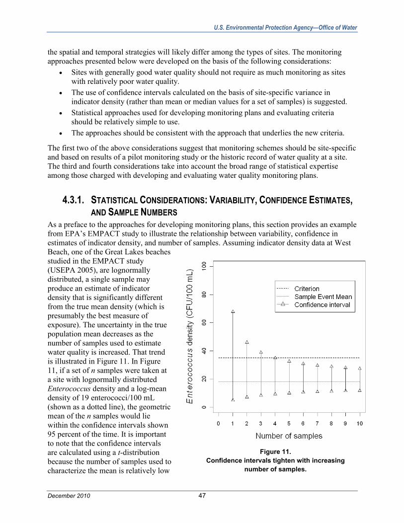
U.S. Environmental Protection Agency—Office of Water
December 2010 47
the spatial and temporal strategies will likely differ among the types of sites. The monitoring approaches presented below were developed on the basis of the following considerations:
• Sites with generally good water quality should not require as much monitoring as sites with relatively poor water quality.
• The use of confidence intervals calculated on the basis of site-specific variance in indicator density (rather than mean or median values for a set of samples) is suggested.
• Statistical approaches used for developing monitoring plans and evaluating criteria should be relatively simple to use.
• The approaches should be consistent with the approach that underlies the new criteria.
The first two of the above considerations suggest that monitoring schemes should be site-specific and based on results of a pilot monitoring study or the historic record of water quality at a site. The third and fourth considerations take into account the broad range of statistical expertise among those charged with developing and evaluating water quality monitoring plans.
4.3.1. STATISTICAL CONSIDERATIONS: VARIABILITY, CONFIDENCE ESTIMATES, AND SAMPLE NUMBERS
As a preface to the approaches for developing monitoring plans, this section provides an example from EPA’s EMPACT study to illustrate the relationship between variability, confidence in estimates of indicator density, and number of samples. Assuming indicator density data at West Beach, one of the Great Lakes beaches studied in the EMPACT study (USEPA 2005), are lognormally distributed, a single sample may produce an estimate of indicator density that is significantly different from the true mean density (which is presumably the best measure of exposure). The uncertainty in the true population mean decreases as the number of samples used to estimate water quality is increased. That trend is illustrated in Figure 11. In Figure 11, if a set of n samples were taken at a site with lognormally distributed Enterococcus density and a log-mean density of 19 enterococci/100 mL (shown as a dotted line), the geometric mean of the n samples would lie within the confidence intervals shown 95 percent of the time. It is important to note that the confidence intervals are calculated using a t-distribution because the number of samples used to characterize the mean is relatively low
Figure 11.
Confidence intervals tighten with increasing number of samples.

U.S. Environmental Protection Agency—Office of Water
December 2010 48
(usually less than 30). Figure 11 shows that to state with 97.5 percent confidence that the observed sample mean is below the criterion (35 enterococci per 100 mL; shown as a dashed line), it would be necessary to take four samples.
Figure 11 shows that when microbial water quality is good, a relatively small number of samples is required to conclude with a given level of confidence that the mean indicator density is below a specified criterion. In this illustration, the criterion is associated with a confidence level. This confidence level accounts for variability inherent at a site and might be selected on the basis of a tradeoff between beach closures and management of human health risk.
In actual practice, the number of samples is likely to vary according to beach characteristics and the sources of pollution at a beach. The analysis of one of the few sets of results from EPA epidemiology studies conducted to assess the relationship between GI illness and qPCR monitoring results has shown that six samples collected at a single sample time are usually sufficient to maintain an adequate correlation with GI illness (Wade et al. 2006).
4.3.2. STATISTICAL CONSIDERATIONS FOR SPATIAL SAMPLING. Building on that background information, several approaches can be used to choose the number of samples taken per sampling event. Those approaches include the following:
• Selecting the number of samples on the basis of a power curve (considering the difference from the criterion that must be detected and the acceptable type I and type II errors).
• Acquiring a composite sample composed of a sufficient number of subsamples to provide a precision approaching some specified value (e.g., an equivalent to a specified number of individual samples).
• Selecting a small number of samples (as few as one) on the basis of economic or other constraints.
The use of a power curve for establishing the number of samples required along a beach per sampling event is described in detail by Wymer (USEPA 2005; Wymer, 2007). Briefly, low (typically 0.05) and high (typically 0.95) acceptable risks are assigned to illness rates above and below the rate selected as acceptable for primary contact recreation. Those low and high indicator illness rates can be converted to indicator densities via health effects relations developed in epidemiological studies, and the resulting indicator densities constitute a tolerance interval or a detectable difference that must be possible with the number of samples selected in a monitoring plan. Assuming the along-shore (between transect) spatial variance, V, at the site has been established through a pilot monitoring study or via adopting a reference value for sites with similar features and fecal pollution sources, the number of samples, n, required to limit type I errors to α and to be consistent with a tolerance interval of L is given by (Devore 1991):
[Equation 3] 21
22
×=
Lzn σα

U.S. Environmental Protection Agency—Office of Water
December 2010 49
where zα is the upper αth percentile of the standard normal distribution. As described above, the spatial variance can be estimated from data from pilot monitoring and can be chosen on the basis of some average variance observed among sampling events or on the basis of a value observed when water quality was marginal.
When inferences are based on a single sample, the tolerance interval cannot be specified but rather will be determined on the basis of type I errors. If estimates of the spatial along-shore variance are based on a relatively small number of samples, the upper confidence level estimate for the indicator density based on a single sample in which the density was found to be x organisms per 100 mL is given by
[Equation 4] σα 2zx +
where x is the log-mean indicator density for the samples and, σ is an estimate standard deviation of the log-transformed densities. Because the number of samples is not chosen consistent with a tolerance interval, the single sample results in a higher incidence of false positives (indicator density assessed as above the standard when it is not) than if more samples were used.
As noted in the discussion of composite samples presented in Section 4.3, the precision of a composite sample can be raised by increasing the number of sub-samples composing the composite sample. So an alternative approach to estimating the sample size via equation 3 is to use a composite sample with a sufficient number of sub-samples to give the same precision as the number of individual samples as calculated in equation 3.
4.3.3. STATISTICAL CONSIDERATIONS FOR TEMPORAL SAMPLING. As noted above, sites are assessed differently and have different temporal sampling requirements. Sampling schemes could be regular, random, or event driven/adaptive. For sites with many swimmers and high economic consequences associated with closing beaches, the objective of sampling is to assess the water quality on the day the sample is drawn. That is particularly relevant for samples analyzed via rapid methods; the value in the rapid method lies in the ability to use information from the sample to inform swimmers of potential water quality problems before (on the day) they swim.
Two temporal sampling approaches appear appropriate for sites with designated beaches: sampling at a regular interval (preferably day) and event-driven sampling. Here, event-driven sampling refers to sampling conducted when a prior indicator measurement, environmental condition at the site, or an anomalous event such as a sewage spill indicate a high potential for exceedance of a target indicator level. Studies that have lead to developing predictive models (e.g., Kinzelman et al. 2004; Nevers and Whitman 2005), which demonstrated that variables such as rainfall, wind direction, wind speed and wave height can account for a significant portion of the variability in observed indicator densities. In event-driven sampling, the occurrence of conditions associated with increased indicator density can be used to trigger sampling. Once samples indicate an exceedance of the target indicator level, the site should be considered out of compliance until a subsequent sample indicates water quality within the target level and event conditions are no longer present. Selecting the level of an environmental variable at which sampling should be triggered can be done on the basis of a pilot sampling study or historical data

U.S. Environmental Protection Agency—Office of Water
December 2010 50
and through use of constructs such as a rainfall rating curve. In a rainfall rating curve, historical indicator densities measured at a site are plotted against rainfall amounts. Ideally, such a curve will demonstrate a clear relationship between indicator density and rainfall in the vicinity of the indicator density of concern.
4.4. SUMMARY OF MONITORING APPROACHES AND CONSIDERATIONS In summary, except at beaches with historical data on both temporal and spatial indicator variability, development of site-specific sampling plans should be considered as part of an approach to site characterization using a sanitary survey and a pilot monitoring study as first steps. Those studies will identify how fecal pollution sources are aligned with respect to the beach and whether any beach features divide the site into hydrologically distinct zones that should be sampled separately. After variability is assessed, one can use several options for spatial and temporal sampling to establish whether water quality meets a specified target.
On the basis of findings from the literature and analyses, summary information is provided below for where to sample, when to sample, and how to sample.
4.4.1. REVIEW OF INDICATOR DENSITY VARIABILITY Indicator densities exhibit high variability at multiple time and length scales. While conditions can cause variability to differ between sites, the relative magnitudes of temporal variations in indicator density for both coastal and inland sites at different time scales are the following:
Event variability refers to the change in indicator density associated with rain events. Among the documented temporal variabilities, event scale variability is, by far, the greatest. Indicator organism density can change multiple logs during a single precipitation event. Indicator loading also varies significantly during rain events, although not necessarily following the same temporal pattern as indicator density variations. Because event variability is so great, beach managers might use alternatives to indicator counts for assessing water quality after and during events. For example, historic rainfall and indicator data might be used to estimate a rainfall depth threshold at which beaches are likely to be out of compliance.
Although site variations can alter the relative dependence of indicator density on sample location, the general dependence of indicator density variability with location for coastal sites is expected to be the following:

U.S. Environmental Protection Agency—Office of Water
December 2010 51
For inland water sites, the variation is expected to be the following:
The physical alignment of both coastal and inland sites with features that promote or inhibit mixing and point sources of fecal indicator organisms plays a significant role in the distribution of indicators at those sites. These features can be identified during a sanitary survey of recreational sites. Site features that appear important to identify during sanitary surveys include the presence of the following:
• Jetties, dams, or other features that influence mixing at a site or promote retention of indicators at a site.
• Point sources, particularly POTW discharges, in the vicinity of the site. • Nonpoint sources, particularly livestock operations and areas where wild birds and
animals congregate, near sites.
4.4.2. WHERE TO SAMPLE Sampling locations should be selected on the basis of the ability of a small number of samples to adequately describe water quality at the site. Site-specific sampling plans should take into account historic water quality and variability and the presence of physical features (point sources, bird nesting areas, structures that influence mixing, and such) known to affect distribution of indicators. Sanitary surveys offer a vehicle for identifying important physical features and an alternative to intensive sampling as a means for assessing spatial variability. In general, samples should be drawn from where water quality can be best characterized. Those are locations where indicator organisms are most likely to be associated with a fecal pollution source (e.g., away from areas where resuspended or indigenous organisms might be suspended) and at locations where variability is not excessive. Such an approach will optimize monitoring such that samples properly reflect the water quality of the site and are related to health effects data.
Where to Sample: Coastal Sites
Water column depth zone. The water column depth zone can be considered an area parallel to the shore where one collects a sample. Taking a sample in the zone where the water depth is approximately knee deep or greater appears to offer some advantages. Indicator density tends to

U.S. Environmental Protection Agency—Office of Water
December 2010 52
vary less in deeper waters than in shallower zones. In addition, correlations between indicator organism density measured at that depth tend to have better correlations with GI illness incidence rates. Indicator density in shallower water is higher than that in deeper areas because of the resuspension of indicator organisms growing or sheltered in sediments. Resuspended indicators might not be indicative of fresh fecal pollution and, therefore, samples with a high number of resuspended organisms might not provide a good means to assess water quality. In some cases, considerations other than the locations for optimal sampling can play a role in selecting the appropriate sample depth zone. In California marine waters, for example, samples are taken at ankle depth in part to protect the safety of the sampler from the threat posed by incoming waves.
Depth of sample collection below surface. Collecting one’s sample near the water surface offers some advantages. The depth for the collection device (i.e., distance below the water surface) appears to be less critical than the depth zone (e.g. knee depth) where sampling is conducted. Some studies have demonstrated higher indicator density near bottom sediments than in overlying waters and their findings support sampling in the top 15 cm (~ 6 inches) of the water column. Additional positive features of sampling near the water surface include ease of sample collection and avoidance of water in the vicinity of sediments where resuspension of indicator bacteria is possible.
Sample locations in the along-shore direction should be chosen on the basis of knowledge of the mixing characteristic of the beach and location of sources of fecal contamination as determined by sanitary surveys. When there are beach features influencing hydrodynamics (mixing), regions of the beach with different hydraulics cannot be expected to have similar indicator densities and, hence, should be sampled separately.
Where to Sample: Inland Sites
For streams, except in the vicinity of point sources, indicator density is expected to vary in the downstream direction (because of indicator inactivation in the water column or resuspension from sediments) and to be higher near the sediments than at the water surface. Sampling of streams within the top 15 cm of water allows characterization of water quality at the most likely site of human exposure and away from resuspended indicator organisms that might not be indicative of recent fecal pollution events. In the downstream direction, monitoring locations can be selected on the basis of knowledge of the location of point and nonpoint sources of pollution.
4.4.3. WHEN TO SAMPLE Collection of samples in the morning appears to offer the best balance between practicality and generation of data that protects human health. If culture methods are used for enumerating indicator bacteria, morning samples could generate results that would allow posting of health advisories the next day or two. If qPCR or other rapid methods are used, the faster evaluation of samples might allow same day notification. However, practical limitations (such as sample transport and other factors) could delay such notifications.
Diurnal variation in indicator density is observed in both inland and coastal waters, with the variation in indicator density possibly higher for coastal sites where there is less shading and greater water surface are than for inland sites.

U.S. Environmental Protection Agency—Office of Water
December 2010 53
In general, when culture methods are used for indicator bacteria enumeration, high indicator densities are observed at least until 8:00 a.m. and perhaps later for some sites. Depending on the insolation on a given day and at a site, the lowest indicator density typically occurs between 2:00 and 3:00 p.m., according to culture results. Such a diurnal trend might not apply to indicator density measurements made using qPCR or might apply to a different extent.
4.4.4. HOW TO SAMPLE Sampling should target areas of beaches in closer proximity to fecal pollution sources and portions of the beach with significantly different mixing should be sampled separately. From a monitoring perspective, the most important information derived from pilot monitoring studies is along-shore spatial variance characteristic for a site. The along-shore variance can be estimated on the basis of an aggregate measure of daily along-shore variances observed during the pilot study or on the basis of a characteristic variance such as the variance observed when water quality is marginal (approaching a level of concern).
Operational beach monitoring could be configured on the basis of (1) a power curve approach (acceptance sampling), with the number of samples selected according to site-specific variance estimate and a tolerance interval selected using a range of tolerable risks and an epidemiological relationship between indicator density and human health effects, or (2) a composite sampling strategy in which the number of samples composited is chosen to provide a precision approaching that associated with the number of samples estimated using the power curve approach. In each case, inferences about water quality are based on comparison of some confidence interval around sampling for a sampling event estimate of variance with a target value. Confidence intervals about sample means are based on site-specific variance estimates derived in site characterization.
With regard to the actual number of samples required to adequately characterize water quality for public health protection at beaches, the number is likely to vary according to beach characteristics and the sources of pollution at a beach.
4.4.5. HOW OFTEN TO SAMPLE Although literature on this topic based on qPCR data is limited to EPA studies and those of a few other researchers, the analysis of the results from EPA’s epidemiology studies conducted to assess the relationship between GI illness and qPCR monitoring results has shown that six samples collected at a single sample time are usually sufficient to maintain an adequate correlation with GI illness. Further research based on the statistical analyses of results from qPCR water quality determinations will be required to further elucidate these relationships.
The available basis for research on all aspects of the representativeness of qPCR sampling results will be augmented by the implementation and widespread use of qPCR for monitoring at recreational beaches. Additional focused statistical analysis of results from qPCR water quality determinations, including qPCR monitoring data from current epidemiology and other studies being and recently conducted by EPA and other agencies, would further inform the temporal, spatial, and statistical basis for sampling requirements for the protection of public health at beaches.

U.S. Environmental Protection Agency—Office of Water
December 2010 54
This page is intentionally blank.

U.S. Environmental Protection Agency—Office of Water
December 2010 55
CHAPTER 5 References Ahn, J.H., S.B. Grant, C.Q. Surbeck, P.M. DiGiacomo, N.P. Nezlin, and S. Jiang. 2005. Coastal
water quality impact of stormwater runoff from an urban watershed in Southern California. Environmental Science and Technology 39(16):5940-5953.
An, Y.J., D.H. Kampbell, and G.P. Breidenbach. 2002. Escherichia coli and total coliforms in water and sediments at lake marinas. Environmental Pollution 120(3):771-778.
Armstrong, I., S. Higham, G. Hudson, and T. Colley. 1996. The Beachwatch pollution monitoring programme: Changing priorities to recognize changed circumstances. Marine Pollution Bulletin 33(7-12):249-259.
Åström, J., T.J. Pettersson, T.A. Stenström, and O. Bergstedt. 2009. Variability analysis of pathogen and indicator loads from urban sewer systems along a river. Water Science and Technology 59(2):203-212.
Baxter-Potter, W.R., and M.W. Gilliland. 1988. Bacterial pollution run-off from agricultural lands. Journal of Environmental Quality 17(1):27-34.
Bertke, E.E. 2007. Composite analysis for Escherichia coli at coastal beaches. Journal of Great Lakes Research 33(2):335-341.
Boehm, A.B. 2003. Model of microbial transport and inactivation in the surf zone and application to field measurements of total coliform in northern Orange County, California. Environmental Science and Technology 37(24):5511-5517.
Boehm, A.B. 2007. Enterococci concentrations in diverse coastal environments exhibit extreme variability. Environmental Science and Technology 41(24):8227-8232.
Boehm, A.B., S.B. Grant, J.H. Kim, S.L. Mowbray, C.D. McGee, C.D. Clark, D.M. Foley, and D.E. Wellman. 2002. Decadal and shorter period variability of surf zone water quality at Huntington Beach, California. Environmental Science and Technology 36(18):3885-3892.
Boehm, A.B., J.A. Fuhrman, R.D. Mrse, and S.B. Grant. 2003. Tiered approach for identification of a human fecal pollution source at a recreational beach: Case study at Avalon Bay, Catalina Island, California. Environmental Science and Technology 37(4):673-680.
Boehm, A.B., D.B. Lluch-Cota, K.A. Davis, C.D. Winant, and S.G. Monismith. 2004. Covariation of coastal water temperature and microbial pollution at interannual to tidal periods. Geophysical Research Letters 31(6).
Boehm, A.B., D.P. Keymer, and G.G. Shellenbarger. 2005a. An analytical model of enterococci inactivation, grazing, and transport in the surf zone of a marine beach. Water Research 39:3565-3578.

U.S. Environmental Protection Agency—Office of Water
December 2010 56
Boehm, A.B., and S.B. Weisberg. 2005b. Tidal forcing of enterococci at marine recreational beaches at fortnightly and semidiurnal frequencies. Environmental Science and Technology 39(15):5575-5583.
Bonilla, T.D., K. Nowosielski, M. Cuvelier, A. Hartz, M. Green, N. Esiobu, D.S. McCorquodale, J.M. Fleisher, and A. Rogerson. 2007. Prevalence and distribution of fecal indicator organisms in South Florida beach sand and preliminary assessment of health effects associated with beach sand exposure. Marine Pollution Bulletin 54(9):1472-1482.
Bordalo, A.A. 2003. Microbiological water quality in urban coastal beaches: The influence of water dynamics and optimization of the sampling strategy. Water Research 37(13):3233-3341.
Brenniman, G.R., S.H. Rosenberg, and R.L. Northrop. 1981. Microbial sampling variables and recreational water quality standards. American Journal of Public Health 71(3):283-289.
Brookes, J.D., M.R. Hipsey, M.D. Burch, R.H. Regel, L.G. Linden, C.M. Ferguson, and J.P. Antenucci. 2005. Relative value of surrogate indicators for detecting pathogens in lakes and reservoirs. Environmental Science and Technology 39(22):8614-8621.
Byappanahalli, M.N., M. Fowler, D. Shively, and R.L. Whitman. 2003. Ubiquity and persistence of Escherichia coli in a midwestern coastal stream. Applied and Environmental Microbiology 69(8):4549-4555.
Canale, R.P., M.T. Auer, E.M. Owens, T.M. Heidtke, and S.W. Effler. 1991. Modeling fecal coliform bacteria - II. Model development and application. Water Research 27(4):703-714.
Carney, J.F., C.E. Carty, and R.R. Colwell. 1975. Seasonal occurrence and distribution of microbial indicators and pathogens in the Rhode River of Chesapeake Bay. Applied and Environmental Microbiology 30(5):771-780.
Chen, C.W., L.E. Gomez, C.L. Chen, and D.B. Jacobsen. 1991. Investigation of beach contamination using tracer. Journal of Environmental Engineering 117(1):101-115.
Cheung, W.H.S., K.C.K. Chang, and R.P.S. Hung. 1991. Variations in microbial indicator densities in beach waters and health-related assessment of bathing water quality. Epidemiology and Infection 106(2):329-344.
Chigbu, P., S. Gordon, and T.R. Strange. 2005. Fecal coliform disappearance rates in a north-central Gulf of Mexico estuary. Estuarine, Coastal and Shelf Science 65(1-2):309-318.
Clarke, L.B., D. Ackerman, and J. Largier. 2007. Dye dispersion in the surf zone: Measurements and simple models. Continental Shelf Research 27:650-669.
Corbett, S.J., G.L. Rubin, G.K. Curry, and D.G. Kleinbaum. 1993. The health effects of swimming at Sydney beaches. The Sydney Beach Users Study Advisory Group. American Journal of Public Health 83(12):1701-1706.
Coulliette, A.D., and R.T. Noble. 2008. Impacts of rainfall on the water quality of the Newport River Estuary (Eastern North Carolina, USA). Journal of Water and Health 6(4):473-482.

U.S. Environmental Protection Agency—Office of Water
December 2010 57
Dan, T.B.-B., and L. Stone. 1991. The distribution of fecal pollution indicator bacteria in Lake Kinneret. Water Research 25(3):263-270.
Davis, K.A., M.A. Anderson, and M.V. Yates. 2005. Distribution of indicator bacteria in Canyon Lake, California. Water Research 39:1277-1288.
Devore, J.L. 1991. Probability and Statistics for Engineering and the Sciences. Duxbury Press, Belmont, CA.
DiDonato, G.T., J.R. Stewart, D.M. Sanger, B.J. Robinson, B.C. Thompson, A.F. Holland, and R.F. Van Dolah. 2009. Effects of changing land use on the microbial water quality of tidal creeks. Marine Pollution Bulletin 58(1):97-106 E-published ahead of print.
Dorner, S.M., W.B. Anderson, T. Gaulin, H.L. Candon, R.M. Slawson, P. Payment, and P.M. Huck. 2007. Pathogen and indicator variability in a heavily impacted watershed. Journal of Water and Health 5(2):241-257.
Edwards, D.R., M.S. Coyne, T.C. Daniel, P.F. Vendrell, J.F. Murdoch, and P.A.J. Moore. 1997. Indicator bacteria concentrations of two northwest Arkansas streams in relation to flow and season. Transactions of the American Society of Agricultural Engineers 40(1):103-109.
Elmanama, A.A., S. Afifi, and S. Bahr. 2006. Seasonal and spatial variation in the monitoring parameters of Gaza Beach during 2002-2003. Environmental Research 101(1):25-33.
Elmir, S.M., M.E. Wright, A. Abdelzaher, H.M. Solo-Gabriele, L.E. Fleming, G. Miller, M. Rybolowik, M.T. Peter Shih, S.P. Pillai, J.A. Cooper, and E.A. Quaye. 2007. Quantitative evaluation of bacteria released by bathers in a marine water. Water Research 41(1):3-10.
Fernández-Molina, M.C., A. Alvarez, and M. Espigares. 2004. Presence of hepatitis A virus in water and its relations with indicators of fecal contamination. Water, Air, and Soil Pollution 159(1):197-208.
Fleisher, J.M. 1985. Implications of coliform variability in the assessment of the sanitary quality of recreational waters. Journal of Hygiene 94(2):193-200.
Fleisher, J.M. 1990. The effects of measurement error on previously reported mathematical relationships between indicator organism density and swimming-associated illness: A quantitative estimate of the resulting bias. International Journal of Epidemiology 19(4):1100-1106.
Gentry, R.W., J.F. McCarthy, A.C. Layton, L.D. McKay, D.E. Williams, S.R. Koirala, and G.S. Sayler. 2006. Escherichia coli loading at or near base flow in a mixed-use watershed. Journal of Environmental Quality 35(6):2244-2249.
Goyal, S.M., C.P. Gerba, and J.L. Melnick. 1977. Occurrence and distribution bacterial indicators and pathogens in canal communities along the Texas coast. Applied and Environmental Microbiology 34(2):139-149.
Grant, S.B., J.H. Kim, B.H. Jones, T.M. Jenkins, J. Wasyl, and C. Cudaback. 2005. Surf-zone entrainment, along-shore transport, and human health implications of pollution from tidal outlets. Journal of Geophysical Research 110:20.

U.S. Environmental Protection Agency—Office of Water
December 2010 58
Haack, S.K., L.R. Fogarty, and C.C. Wright. 2003. Escherichia coli and Enterococci at beaches in the Grand Traverse Bay, Lake Michigan: Sources, characteristics, and environmental pathways. Environmental Science and Technology 37(15):3275-3283.
Haramoto, E., H. Katayama, K. Oguma, Y. Koibuchi, H. Furumai, and S. Ohgaki. 2006. Effects of rainfall on the occurrence of human adenoviruses, total coliforms, and Escherichia coli in seawater. Water Science and Technology 54(3):225-230.
Haugland, R.A., S.C. Siefring, L.J. Wymer, K.P. Brenner, and A.P. Dufour. 2005. Comparison of Enterococcus measurements in freshwater at two recreational beaches by quantitative polymerase chain reaction and membrane filter culture analysis. Water Research 39(4):559-568.
He, L.-M., J. Lu, and W. Shi. 2007. Variability of fecal indicator bacteria in flowing and ponded waters in Southern California: Implications for bacterial TMDL development and implementation. Water Research 41(14):3132-3140.
Heaney, C.D., E. Sams, S. Wing, S. Marshall, K. Brenner, A.P. Dufour, and T.J. Wade. 2009. Contact with beach sand among beachgoers and risk of illness. American Journal of Epidemiology 170(2):164-172.
Hose, G.C., G. Gordon, F.E. McCullough, N. Pulver, and B.R. Murray. 2005. Spatial and rainfall related patterns of bacterial contamination in Sydney Harbour Estuary. Journal of Water and Health 3(4):349-358.
Jamieson, R.C., D.M. Joy, H. Lee, R. Kostaschuk, and R.J. Gordon. 2005. Resuspension of sediment-associated Escherichia coli in a natural stream. Journal of Environmental Quality 34:581-589.
Jin, G., A.J. Englande, and A. Liu. 2003. A preliminary study on coastal water quality monitoring and modeling. Journal of Environmental Science and Health, Part A Toxic/Hazardous Substances and Environmental Engineering 38(3):493-509.
Kay, D., J. Bartram, A. Prüss, N. Ashbolt, M.D. Wyer, J.M. Fleisher, L. Fewtrell, A. Rogers, and G. Rees. 2004. Derivation of numerical values for the World Health Organization guidelines for recreational waters. Water Research 38(5):1296-1304.
Kim, J.H., and S.B. Grant. 2004. Public mis-notification of coastal water quality: A probabilistic evaluation of posting errors at Huntington Beach, California. Environmental Science and Technology 38(9):2497-2504.
Kinzelman, J., S.L. McLellan, A.D. Daniels, S. Cashin, A. Singh, S. Gradus, and R. Bagley. 2004. Non-point source pollution: Determination of replication versus persistence of Escherichia coli in surface water and sediments and correlation of levels to readily measurable environmental parameters. Journal of Water and Health 2(2):103-114.
Kleinheinz, G.T., C.M. McDermott, M.C. Leewis, and E. Englebert. 2006. Influence of sampling depth on Escherichia coli concentrations in beach monitoring. Water Research 40(20):3831-3837.

U.S. Environmental Protection Agency—Office of Water
December 2010 59
Koirala, S.R., R.W. Gentry, E. Perfect, J.S. Schwartz, and G.S. Sayler. 2008. Temporal variation and persistence of bacteria in streams. Journal of Environmental Quality 37(4):1559-1566.
Le Fevre, N.M., and G.D. Lewis. 2003. The role of resuspension in enterococci distribution in water at an urban beach. Water Science and Technology 47(3):205-210.
Leecaster, M.K., and S.B. Weisberg. 2001. Effect of sampling frequency on shoreline microbiology assessments. Marine Pollution Bulletin 42(11):1150-1154.
Liu, L., M.S. Phanikumar, S.L. Molloy, R.L. Whitman, D.A. Shively, M.B. Nevers, D.J. Schwab, and J.B. Rose. 2006. Modeling the transport and inactivation of E. coli and enterococci in the near-shore region of Lake Michigan. Environmental Science and Technology 40(16):5022-5028.
Masopust, P. 2005. High-Resolution spatial and Temporal Variability and Patterns of Escherichia coli in the Charles River. Master of Science thesis. Northeastern University, Civil and Environmental Engineering. Boston, MA.
McDonald, A., D. Kay, and T. Jenkins. 1982. Generation of fecal and total coliform surges by stream flow manipulation in the absence of normal hydrometeorological stimuli. Applied and Environmental Microbiology 44(2):292-300.
Meays, C.L., K. Broersma, R. Nordin, A. Mazumder, and M. Samadpour. 2006. Diurnal variability in concentrations and sources of Escherichia coli in three streams. Canadian Journal of Microbiology 52(11):1130-1135.
Menon, P., G. Billen, and P. Servair. 2003. Mortality rates of autochthonous and fecal bacteria in natural aquatic systems. Water Research 37:4151-4158.
Mill, A., T. Schlacher, and M. Katouli. 2006. Tidal and longitudinal variation of fecal indicator bacteria in an estuarine creek in south-east Queensland, Australia. Marine Pollution Bulletin 52:881-891.
Nevers, M.B., and R.L. Whitman. 2005. Nowcast modeling of Escherichia coli concentrations at multiple urban beaches of southern Lake Michigan. Water Research 39(20):5250-5260.
Noble, R.T., S.B. Weisberg, M.K. Leecaster, C.D. McGee, J.H. Dorsey, P. Vainik, and V. Orozco-Borbon. 2003. Storm effects on regional beach water quality along the Southern California shoreline. Journal of Water and Health 1(1):23-31.
Noble, M.A., J.P. Xu, L.K. Rosenfeld, C.D. McGee, and G.L. Robertson. 2005. Temporal and spatial patterns for surf zone bacteria before and after disinfection of the Orange County sanitation district effluent. Oceans 1-3:382-387.
Obiri-Danso, K., and K. Jones. 1999. Distribution and seasonality of microbial indicators and thermophilic campylobacters in two freshwater bathing sites on the River Lune in northwest England. Journal of Applied Microbiology 87(6):822-832.
Olyphant, G.A., and R.L. Whitman. 2004. Elements of a predictive model for determining beach closures on a real time basis: The case of 63rd Street Beach Chicago. Environmental Monitoring and Assessment 98(1-3):175-190.

U.S. Environmental Protection Agency—Office of Water
December 2010 60
Parkhurst, D.F., K.P. Brenner, A.P. Dufour, and L.J. Wymer. 2005. Indicator bacteria at five swimming beaches—Analysis using random forests. Water Research 39(7):1354-1360.
Pednekar, A.M., S.B. Grant, Y. Jeong, Y. Poon, and C. Oancea. 2005. Influence of climate change, tidal mixing, and watershed urbanization on historical water quality in Newport Bay, a saltwater wetland and tidal embayment in Southern California. Environmental Science and Technology 39(23):9071-9082.
Petersen, T.M., H.S. Rifai, M.P. Suarez, and A.R. Stein. 2005. Bacteria loads from point and nonpoint sources in an urban watershed. Journal of Environmental Engineering 131(10):1414-1425.
Petersen, T.M., M.P. Suarez, H.S. Rifai, P. Jensen, Y.C. Su, and R. Stein. 2006. Status and trends of fecal indicator bacteria in two urban watersheds. Water Environment Research 78(12):2340-2355.
PHLS Water Surveillance Group. 1995. Preliminary study of microbiological parameters in eight inland recreational waters. Letters in Applied Microbiology 21(4):267-271.
Reischer, G.H., J.M. Haider, R. Sommer, H. Stadler, K.M. Keiblinger, R. Hornek, W. Zerobin, R.L. Mach, and A.H. Farnleitner. 2008. Quantitative microbial faecal source tracking with sampling guided by hydrological catchment dynamics. Environmental Microbiology 10(10):2598-2608.
Roll, B.M., and R.S. Fujioka. 1997. Sources of faecal indicator bacteria in a brackish, tropical stream and their impact on recreational water quality. Water Science and Technology 35(11-12):179-186.
Rosenfeld, L.K., C.D. McGee, G.L. Robertson, M.A. Noble, and B.H. Jones. 2006. Temporal and spatial variability of fecal indicator bacteria in the surf zone off Huntington Beach, CA. Marine Environmental Research 61(5):471-93.
Ryu, H., A. Alum, M. Alvarez, J. Mendoza, and M. Abbaszadegan. 2005. An assessment of water quality and microbial risk in Rio Grande Basin in the United States-Mexican border region. Journal of Water and Health 3(2):209-218.
Santoro, A.E., and A.B. Boehm. 2007. Frequent occurrence of the human-specific Bacteroides fecal marker at an open coast marine beach: Relationship to waves, tides and traditional indicators. Environmental Microbiology 9(8):2038-2049.
Sayler, G.S., J.D. Nelson Jr., A. Justice, and R.R. Colwell. 1975. Distribution and significance of fecal indicator organisms in the Upper Chesapeake Bay. Applied and Environmental Microbiology 30(4):625-638.
Seyfried, P.L., R.S. Tobin, N.E. Brown, and P.F. Ness. 1985. A prospective study of swimming-related illness. II. Morbidity and the microbiological quality of water. American Journal of Public Health 75(9):1071-1075.
Shanks, O.C., C. Nietch, M. Simonich, M. Younger, D. Reynolds, and K.G. Field. 2006. Basin-wide analysis of the dynamics of fecal contamination and fecal source identification in Tillamook Bay, Oregon. Applied and Environmental Microbiology 72(8):5537-5546.

U.S. Environmental Protection Agency—Office of Water
December 2010 61
Shehane, S.D., V.J. Harwood, J.E. Whitlock, and J.B. Rose. 2005. The influence of rainfall on the incidence of microbial faecal indicators and the dominant sources of faecal pollution in a Florida river. Journal of Applied Microbiology 98(5):1127-1136.
Sinton, L.W., C.H. Hall, P.A. Lynch, and R.J. Davies-Colley. 2002. Sunlight inactivation of fecal indicator bacteria and bacteriophages from waste stabilization pond effluent in fresh and saline waters. Applied and Environmental Microbiology 68(3):1122-1131.
Stevenson, A.H. 1953. Studies of bathing water quality and health. American Journal of Public Health 45:529-539.
Tiefenthaler, L.L., E.D. Stein, and G.S. Lyon. 2009. Fecal indicator bacteria (FIB) levels during dry weather from Southern California reference streams. Environmental Monitoring and Assessment 155(1-4):477-492.
Traister, E., and S.C. Anisfeld. 2006. Variability of indicator bacteria at different time scales in the Upper Hoosic River watershed. Environmental Science and Technology 40(16):4990-4995.
Trowbridge, P.R., and S.H. Jones. 2009. Detecting water quality patterns in New Hampshire’s estuaries using National Coastal Assessment probability-based survey data. Environmental Monitoring and Assessment 150(1-4):129-142.
Turbow, D.J., N.D. Osgood, and S.C. Jiang. 2003. Evaluation of recreational health risk in coastal waters based on Enterococcus densities and bathing patterns. Environmental Health Perspectives 111(4):598-603.
USEPA (U.S. Environmental Protection Agency). 1983. Health Effects Criteria for Marine Recreational Waters. EPA-600/1-80-031 U.S. Environmental Protection Agency, Cincinnati, OH.
USEPA (U.S. Environmental Protection Agency).1984. Health Effects Criteria for Fresh Recreational Waters. EPA-600-1-84-004 U.S. Environmental Protection Agency, Office of Research and Development, Cincinnati, OH.
USEPA (U.S. Environmental Protection Agency). 1986. Ambient Water Quality for Bacteria. EPA440/5-84-002 U.S. Environmental Protection Agency, Washington, DC.
USEPA (U.S. Environmental Protection Agency). 2002a. Environmental Monitoring for Public Access and Community Tracking (EMPACT) Beaches Project: Time-Relevant Beach and Recreational Water Quality Monitoring and Reporting. EPA/625/R-02/017 U.S. Environmental Protection Agency, Washington, DC.
USEPA (U.S. Environmental Protection Agency). 2002b. National Beach Guidance and Required Performance Criteria for Grants. EPA-823-B-02-004 U.S. Environmental Protection Agency, Washington DC.
USEPA (U.S. Environmental Protection Agency). 2004. Water Quality Standards for Coastal and Great Lakes Recreation Water. Federal Register 69(220): 67217-67243. U.S. Environmental Protection Agency.

U.S. Environmental Protection Agency—Office of Water
December 2010 62
USEPA (U.S. Environmental Protection Agency). 2005. EMPACT Beaches Project: Results from a Study on Microbiological Monitoring in Recreational Waters. EPA 600/R-04/023 U.S. Environmental Protection Agency, Office of Research and Development, National Exposure Research laboratory, Cincinnati, OH.
USEPA (U.S. Environmental Protection Agency). 2006a. Water Quality Standards For Coastal Recreation Waters: Considerations for States as They Select Appropriate Risk Levels. EPA-823-F-06-012 U.S. Environmental Protection Agency, Washington, DC.
USEPA (U.S. Environmental Protection Agency). 2006b. Water Quality Standards for Coastal Recreation Waters: Acceptable Risk Levels in Great Lakes Waters. EPA-823-F-06-013 U.S. Environmental Protection Agency, Washington, DC.
USEPA (U.S. Environmental Protection Agency). 2007a. Critical Path Science Plan for Development of New of Revised Recreational Water Quality Criteria. EPA 823-R-08-002 U.S. Environmental Protection Agency, Washington, DC.
USEPA (U.S. Environmental Protection Agency). 2008. Great Lakes Beach Sanitary Survey User Manual. EPA-823-B-06-001 U.S. Environmental Protection Agency, Office of Water, Washington, DC.
Vidon, P., L.P. Tedesco, J. Wilson, M.A. Campbell, L.R. Casey, and M. Gray. 2008. Direct and indirect hydrological controls on E. coli concentration and loading in midwestern streams. Journal of Environmental Quality 37(5):1761-1768.
Wade, T.J., R.L. Calderon, E. Sams, M. Beach, K.P. Brenner, A.H. Williams, and A.P. Dufour. 2006. Rapidily measured indicators of recreational water quality are predictive of swimming-associated gadtrointestinal illness. Environmental Health Perspectives 114(1):24-28.
Wade, T.J., R.L. Calderon, K.P. Brenner, E. Sams, M. Beach, R.A. Haugland, L. Wymer, and A.P. Dufour. 2008. High sensitivity of children to swimming-associated gastrointestinal illness. Epidemiology 19(3):375-383.
Walters, S.P., K.M. Yamahara, and A.B. Boehm. 2009. Persistence of nucleic acid markers of health-relevant organisms in seawater microcosms: Implications for their use in assessing risk in recreational waters. Water Research 43(19):4929-4939.
Whitman, R.L., M.B. Nevers, G.C. Korinek, and M.N. Byappanahalli. 2004a. Solar and temporal effects on Escherichia coli concentration at a Lake Michigan swimming beach. Applied and Environmental Microbiology 70(7):4276-4285.
Whitman, R.L., and M.B. Nevers. 2004b. Escherichia coli sampling reliability at a frequently closed Chicago Beach: Monitoring and management implications. Environmental Science and Technology 38(16):4241-6.
Whitman, R.L., M.B. Nevers, and M.N. Byappanahalli. 2006. Examination of the watershed-wide distribution of Escherichia coli along southern Lake Michigan: An integrated approach. Applied and Environmental Microbiology 72(11):7301-7310.

U.S. Environmental Protection Agency—Office of Water
December 2010 63
Whitman, R.L., and M.B. Nevers. 2008. Summer E. coli patterns and responses along 23 Chicago beaches. Environmental Science and Technology 42(24):9217-9224.
Wyer, M.D., D. Kay, G.F. Jackson, H.M. Dawson, J. Yeo, and L. Tanguy. 1995a. Indicator organism sources and coastal water quality: A catchment study on the island of Jersey. Journal of Applied Bateriology 78(3):290-296.
Wymer, L. 2007. The lognormal distribution and use of the geometric mean and arithmetic mean in recreational water quality measurement In Statistical Framework for Recreational Quality Criteria and Modeling, pp. 91-112. John Wiley and Sons, West Sussex, U.K.
Yamahara, K.M., A.C. Layton, A.E. Santoro, and A.B. Boehm. 2007. Beach sands along the California coast are diffuse sources of fecal bacteria to coastal waters. Environmental Science and Technology 41:4515-4521.