Saline groundwater – surface water interaction in coastal

Saline groundwater – surface water interaction in coastal lowlands

Joost R. Delsman

© 2015 Joost Reinbert Delsman and IOS Press

All rights reserved. No part of this book may be reproduced, stored in a retrieval system, or transmitted, in any form or by any means, without prior written permission from the publisher.

Reuse of the knowledge and information in this publication is welcomed on the understanding that due credit is given to the source. However, neither the publisher nor the author can be held responsible for any consequences resulting from such use.

ISBN 978-1-61499-517-3 (print)ISBN 978-1-61499-518-0 (online)DOI 10.3233/978-1-61499-518-0-i

PublisherIOS Press BVNieuwe Hemweg 6B1013 BG AmsterdamNetherlandsfax: +31 20 687 0019e-mail: [email protected]

Distributor in the USA and CanadaIOS Press, Inc.4502 Rachael Manor DriveFairfax, VA 22032USAfax: +1 703 323 3668e-mail: [email protected]

PRINTED IN THE NETHERLANDS

VRIJE UNIVERSITEIT

Saline groundwater – surface water interaction in coastal lowlands

ACADEMISCH PROEFSCHRIFT

ter verkrijging van de graad Doctor aan

de Vrije Universiteit Amsterdam,

op gezag van de rector magnificus

prof.dr. F.A. van der Duyn Schouten,

in het openbaar te verdedigen

ten overstaan van de promotiecommissie

van de Faculteit der Aard- en Levenswetenschappen

op maandag 15 juni 2015 om 15.45 uur

in de aula van de universiteit,

De Boelelaan 1105

door

Joost Reinbert Delsman

geboren te Waalwijk

promotor: prof.dr. P.J. Stuijfzand

copromotoren: dr.ir. G.H.P. Oude Essink dr. J. Groen

Thesis committee: prof.dr.ir. N.C. van de Giessen prof.dr. habil. S. Uhlenbrook prof.dr.ir. M.F.P. Bierkens prof.dr.ir. S.E.A.T.M. van der Zee dr. H.P. Broers

VII

Contents

1 Introduction ................................................................................................................................... 1Motivation ...................................................................................................................................................2Hydrology of polder catchments in the Netherlands ..........................................................................4Surface water salinization ........................................................................................................................6Thesis objective and research questions ...............................................................................................9Thesis outline ........................................................................................................................................... 11

2 Paleo-modeling of coastal saltwater intrusion during the Holocene: ............................ 13 an application to the Netherlands

Abstract ..................................................................................................................................................... 14Introduction ............................................................................................................................................. 15Site description ........................................................................................................................................ 17Results ....................................................................................................................................................... 23Discussion ................................................................................................................................................. 30Conclusion ................................................................................................................................................ 33Acknowledgments .................................................................................................................................. 33

3 Investigating summer flow paths in a Dutch agricultural field using .............................. 35high frequency direct measurementsAbstract ..................................................................................................................................................... 36Introduction ............................................................................................................................................. 37Materials and Methods .......................................................................................................................... 38Results ....................................................................................................................................................... 46Discussion ................................................................................................................................................. 60Conclusion ................................................................................................................................................ 63Acknowledgements ................................................................................................................................ 63Appendix: EC - Total Dissolved Solids (TDS) Conversion ................................................................. 64

4 Uncertainty estimation of end-member mixing using generalized likelihood ............. 67 uncertainty estimation (GLUE), applied in a lowland catchment

Abstract ..................................................................................................................................................... 68Introduction ............................................................................................................................................. 69Materials and Methods .......................................................................................................................... 71Results ....................................................................................................................................................... 79Discussion ................................................................................................................................................. 86Conclusion ................................................................................................................................................ 88Acknowledgments .................................................................................................................................. 88

VIII

5 The value of diverse observations in conditioning a real-world field-scale ................... 91 groundwater flow and transport model

Abstract ..................................................................................................................................................... 92Introduction ............................................................................................................................................. 93Methods .................................................................................................................................................... 94Results ..................................................................................................................................................... 100Discussion and Conclusions................................................................................................................ 114Acknowledgements .............................................................................................................................. 116

6 Fast calculation of groundwater exfiltration salinity in a lowland catchment .............119 using a lumped celerity / velocity approach

Abstract ................................................................................................................................................... 120Introduction ........................................................................................................................................... 121Study area and previous modeling ................................................................................................... 122Model description ................................................................................................................................. 125Model application ................................................................................................................................ 130Results ..................................................................................................................................................... 132Discussion ............................................................................................................................................... 136

7 Synthesis and outlook .............................................................................................................139Introduction ........................................................................................................................................... 140Synthesis ................................................................................................................................................. 141Recommendations for further research ........................................................................................... 146

8 Implications for freshwater management in the Netherlands ........................................151Introduction ........................................................................................................................................... 152Surface water flushing ......................................................................................................................... 154Modeling surface water salinization ................................................................................................. 157

References ......................................................................................................................................... 159

Summary ........................................................................................................................................... 177

Samenvatting ................................................................................................................................... 179

Dankwoord ........................................................................................................................................ 181

Curriculum Vitae ............................................................................................................................... 183

List of publications .......................................................................................................................... 184

CHAPTER1Introduction

2

Chapter 1

MoTIVaTIoN

About one quarter of the global population lives in the vicinity of the world’s coastlines, owing to easy access to transport connections and fish stocks, fertile inlands and mild relief [Nicholls and Small, 2002]. Population in these areas is largely dependent on fresh groundwater resources, for domestic, industrial and agricultural use. Groundwater in coastal areas is, however, often saline, as a result of sea water intrusion [Werner et al., 2013], often exacerbated by over-exploitation of coastal aquifers [Custodio and Bruggeman, 1987], past marine transgressions [Stuyfzand and Stuurman, 1994; Post and Kooi, 2003], sea spray [Custodio, 1992], infiltration of saline surface water [Smith and Turner, 2001], or intrusion after catastrophic storm surges or tsunamis [Illangasekare et al., 2006; Oude Essink et al., 2014]. As water is considered non-potable at chloride concentrations of over 0.25 g/L [EU, 1998], and most crops require salinities (total dissolved solids, TDS) of under 2 g/L [Tanji and Kielen, 2002], only 1 – 5% mixing with sea water (average sea water salinity is 35 g/L) suffices to render groundwater unfit for domestic or agricultural use.

increasingpopulationdensity

subsidenceover-extraction

over-extraction

decreasingriver discharges

sea level rise

salt water

intrusion

upconing

salt waterintrusion

saline groundwaterexfiltration

economicdevelopment

increased evapotranspiration

saline

paleo-water

Figure 1.1 | Overview of threats to coastal aquifers.

The salinization of coastal aquifers is therefore a growing concern, especially given the prospects of global change [Ferguson and Gleeson, 2012]. Increasing population density, continuing economic development and urbanization, temperature increase and the resulting sea level rise (SLR) and changing precipitation patterns [IPCC, 2013] are likely to influence coastal aquifers in a myriad of

1

3

Introduction

ways (Figure 1.1) [Ferguson and Gleeson, 2012; Taylor et al., 2013; Van Lanen et al., 2013]. Increasing coastal population densities and economic development increase the need for freshwater [Wada et al., 2013a, 2013b]. Unless properly managed, this increased need will cause over-exploitation of aquifers and the subsequent salinization of extraction wells [Custodio, 2002]. Over-exploitation of aquifers, along with increased drainage, additionally accelerates soil subsidence [Showstack, 2014] and increases sea water intrusion along coastal margins. Temperature rise increases evapotranspiration [IPCC, 2013], both locally, increasing agricultural water demand, and upstream, decreasing river discharges delivering freshwater to coastal areas [Forzieri et al., 2014]. Sea level rise increases the intrusion of sea water in coastal aquifers [Werner and Simmons, 2009; Ferguson and Gleeson, 2012]. In addition, the long memory of groundwater systems ensures the continuing effects of past stresses to coastal aquifers, for instance doubling the exfiltration of salts in the coastal region of the Netherlands over the coming century as a result of past land reclamation and drainage activities [Oude Essink et al., 2010]. In low elevation areas, where hydraulic gradients ensure the upward flow of groundwater, saline groundwater may move toward the ground surface and eventually exfiltrate to surface water. This situation is not uncommon in deltaic coastal areas, where increased (artificial) drainage has lowered the land surface to elevations below mean sea level (m.s.l.). Notable examples can be found in the Mississippi delta in Louisiana, USA, the Ganges-Brahmaputra delta in Bangladesh, or the Rhine-Meuse delta in the Netherlands. Surface water is generally readily available in low-lying delta areas and is therefore often the prime source of water for drinking water production, and agricultural and industrial use. In addition, surface water supports vital, freshwater-dependent aquatic ecosystems. The exfiltration of saline groundwater may render receiving surface waters unfit for the above purposes and threaten its supported functions. Climate change will likely increase surface water salinization, as decreasing freshwater recharge and increasing upward flow of saline groundwater increase the shallow occurrence and exfiltration of saline groundwater [De Louw et al., 2011a]. However, the hydrological processes and physiographic factors that control saline groundwater exfiltration are not fully understood, hampering successful mitigation strategies. Understanding the exfiltration of saline groundwater to surface water is therefore the prime objective of this thesis.In the Netherlands, about one-quarter of the country is situated below m.s.l.. The Netherlands may in that sense be regarded a laboratory for vulnerable coastal areas worldwide, at risk of sinking below m.s.l. due to the combined effects of soil subsidence and SLR [Showstack, 2014] . Exfiltration of saline groundwater is indeed common throughout the coastal region of the Netherlands [Van Rees Vellinga et al., 1981; De Louw, 2013]. Salinization of surface water is commonly mitigated by flushing of ditches and canals with extraneous freshwater, diverted from the rivers Rhine and Meuse, during the agricultural growing season. Both the projected decrease of freshwater availability from these rivers [Forzieri et al., 2014] and increase of surface water salinization [Oude Essink et al., 2010] threaten the sustainability of current water management practice, and prompted water managers to seek alternative strategies [Delta Programme Commissioner, 2013]. The research presented in this thesis focuses on the Netherlands, given the common occurrence of saline groundwater exfiltration, and the immediate need for alternative mitigation strategies.

4

Chapter 1

HyDRoLoGy oF PoLDER CaTCHMENTS IN THE NETHERLaNDS

Polders are artificially drained, embanked tracts of low elevated land. Totaling around 3000 nationwide, they are a common occurrence in the Netherlands. While the Netherlands are most commonly associated with polders, polders are found in coastal areas across the world. Other European examples are located in Belgium, Germany, France, UK, Italy, Slovenia, Poland and Lithuania, but polders can also be found in Bangladesh, India, Korea, Japan, Guyana, Canada and USA [Wikipedia, 2014]. Polders originated as reclaimed lakes, embanked floodplains or embanked and drained marshlands. Either because by nature of their origin as lake beds, or due to post-embankment soil subsidence relative to their surroundings, surface elevation of polders is generally situated below the surrounding area. This low elevation necessitates the artificial drainage of excess water by means of pumps, or sluices that only operate during low tides. Dutch history of water management started as early as 800 AD, marked by the drainage of coastal salt marshes; embanking floodplains, thus creating the first polders, started around 1000 AD [Pons et al., 1973; Van de Ven, 1993]. Lake reclamation occurred in three separate periods, driven by the availability of technology and the economic situation [Schultz, 1992]. Windmills were used for widespread lake reclamation in the 17th century; the introduction of steam-powered pumps allowed the reclamation of larger and deeper lakes, and gave rise to a second period of lake reclamation in the 19th century. The reclaimed lakes studied in this thesis (Figure 1.5), Schermer (reclaimed in 1635 AD) and Haarlemmermeer (1852 AD), stemmed from these two periods respectively. Land surface elevation in reclaimed polders is generally significantly lower than in other polders. A final period in the 20th century saw the reclamation of large tracts of the IJsselmeer [Schultz, 1992], but land reclamation (e.g., for the expansion of Amsterdam, or the harbor of Rotterdam) continues to this day. The geohydrological situation in Dutch polders can be generalized to a leaky confining layer of Holocene clayey and peaty deposits, overlying an aquifer of Pleistocene sands (Figure 1.2) [Van der Meulen et al., 2013]. Dominant land use in polders is still mostly agriculture, although ongoing urbanization and economic development have had a pronounced impact. A dense network of artificial ditches and canals drains the Holocene confining layer; water is subsequently pumped out from the polder onto the “boezem”, a receiving system of canals. Polders are hydrologically semi-enclosed entities; surface water is exchanged with the boezem through artificial hydraulic structures (pumps, weirs, sluices), additionally a significant regional groundwater flux either enters or exits the polder. Reclaimed, and hence deep, polders experience a significant groundwater inflow, generally in the same order of magnitude as the precipitation surplus [Van Rees Vellinga et al., 1981]. Polder water levels are controlled within a narrow margin; the maintained level is generally lower in winter (to buffer discharge peaks) than in summer (to increase water availability). Water from the boezem is diverted into polders to replenish precipitation deficits during the growing season, roughly from April to October. Polders experiencing water quality problems, mostly due to the exfiltration of saline groundwater, additionally take in water from the boezem to flush and dilute the salinity levels in its waterways. The boezem acts as a collector system, and either discharges the collective polder discharges to the main rivers or directly to the sea, or takes in water from the main rivers to replenish water shortages.

1

5

Introduction

intakeculvert

intakeculvert

pump

polder

Pleistocene aquife

r

Holocene confining layer

upward groundwater flow

boezemcanal polder

polder

tile drainage

Figure 1.2 | Schematic overview of polder-boezem system.

The prevailing paradigm governing water management in the Netherlands has gradually shifted over the past decades. This paradigm shift was driven by increasing awareness of the present and climate change-related future vulnerability of the water system to flooding, water scarcity and water quality problems [van der Brugge et al., 2005]. A traditional engineering perspective historically prevailed in water management with a strong focus on optimally supporting water-related functions. This perspective was reflected in, for instance, the tightly controlled water levels and large drainage depths in agricultural regions, and in the widespread channel straightening of brooks and rivers. These measures resulted, however, in increased soil subsidence, accelerated runoff and discharge peaks, decreased soil water storage, increased nutrient loads and a generally poor ecological status. In response, water management focus has shifted to improving the general resilience of the water system, introducing the “retain-store-discharge” water management paradigm in 2000 [Ministerie van Verkeer en Waterstaat, 2000]. The “Delta Programme” was initiated in 2012 to anticipate possible consequences of climate change on water management and to design possible adaptation strategies, considering both flood safety and freshwater availability [Delta Programme Commissioner, 2013].

6

Chapter 1

SURFaCE waTER SaLINIzaTIoN

Various sources contribute to surface water salinity. Sea water intrusion in rivers, the landward migration of a saltwater wedge due to density differences, is the major salinity source in open water estuaries [Savenije, 2005]. Where ship locks separate salt and freshwater, salt creep through locks still presents a significant input of salt in the river system unless additional measures are implemented [Keetels et al., 2011]. Further inputs derive from the upstream weathering of rocks and anthropogenic sources, such as agricultural fertilizer use, salt mining and other industrial waste discharges and waste water treatment plant effluent [Buhl et al., 1991]. In polder-boezem systems in the coastal zone of the Netherlands, however, exfiltration of brackish to saline groundwater presents the main input of salts to the surface water system [Van Rees Vellinga et al., 1981; De Louw et al., 2010]. In these areas, surface water salinity is therefore closely linked to the distribution of salts in groundwater.

Paleo-geography and groundwater salinityThe classic conceptualization of the occurrence of saline coastal groundwater considers a steady-state sharp-interfaced saltwater wedge underlying fresh groundwater and extending inland from the present-day coastline [e.g., Henry, 1959; Custodio and Bruggeman, 1987]. This steady-state conceptualization is, however, increasingly recognized to be an oversimplification of the transient processes dominating coastal margins [Werner et al., 2013]. Heterogeneity in the subsurface [Simmons et al., 2001] fluid density variations occur because of changes in the solute or colloidal concentration, temperature, and pressure of the groundwater. These include seawater intrusion, high-level radioactive waste disposal, groundwater contamination, and geothermal energy production. When the density of the invading fluid is greater than that of the ambient one, density-driven free convection can lead to transport of heat and solutes over larger spatial scales and significantly shorter time scales than compared with diffusion alone. Beginning with the work of Lord Rayleigh in 1916, thermal and solute instabilities in homogeneous media have been studied in detail for almost a century. Recently, these theoretical and experimental studies have been applied in the study of groundwater phenomena, where the assumptions of homogeneity and isotropy rarely, if ever, apply. The critical role that heterogeneity plays in the onset as well as the growth and/or decay of convective motion is discussed by way of a review of pertinent literature and numerical simulations performed using a variable-density flow and solute transport numerical code. Different styles of heterogeneity are considered and range from continuously \”trending\” heterogeneity (sinusoidal and stochastic permeability distributions, dispersive and kinematic mixing along the interface [Lu et al., 2009; De Louw et al., 2013b], tidal and wave run-up effects [Vandenbohede and Lebbe, 2006; Pauw et al., 2014b], geochemical reactions [Moore, 1999], and episodic events like storm surges and tsunamis [Illangasekare et al., 2006] all influence the distribution of fresh and saline groundwater in coastal aquifers. Moreover, migrating coastlines during the Quaternary have significantly impacted coastal aquifers, resulting in both the common occurrence of saline water far inland [Van Weert et al., 2009], and in considerable fresh groundwater reserves offshore [Post et al., 2013]. Salinity in the coastal groundwater of the Netherlands has been shown to predominantly derive from sea water infiltration during Holocene marine transgressions [Stuyfzand, 1993; Post and Kooi, 2003; Post et al., 2003; Post, 2004] and is therefore closely linked to the paleo-geographic evolution

1

7

Introduction

of the coastal zone. Rising sea levels during the Holocene progressively shifted the coastline landward, until the present-day coastline was exceeded around 6500 BC; maximum extent of marine transgression was reached around 3850 BC. Duration of marine inundation was long enough to enable widespread salinization of underlying aquifers by free-convective infiltration of seawater [Kooi et al., 2000; Post and Kooi, 2003]. Sediment availability subsequently began to match the decreasing rate of sea level rise, causing a shift to a prograding coastline [Vos et al., 2011]. The development of sand barriers and dunes prevented flooding in the central and later southern parts of the Dutch coast, allowing meteoric recharge to freshen the hinterland and promoting the widespread accumulation of peat. Subsequent inundations around 800 AD renewed marine conditions in the southern part of the coastline. Marine conditions in the North and South prevailed to around 1500 AD [Vos et al., 2011]. Peat development was at a maximum around 1000 AD, reaching a maximum thickness of 6 m (elevation of 2 m m.s.l.) [Vos, 1998]; hydraulic gradients promoted the infiltration of meteoric water [Stuyfzand, 1993]. Anthropogenic drainage and peat mining subsequently resulted in rapid degradation of these peat deposits and soil subsidence. Anthropogenic influence grew in importance from 1500 AD onwards, through land cultivation, improved agricultural drainage, river embankment, land reclamation and urban development.

Groundwater – surface water interaction and the exfiltration of saline groundwaterPrecipitation follows a variety of flow routes before it enters the surface water system [Sophocleous, 2002]. It directly enters the surface water system, is intercepted by vegetation and subsequently evaporates, infiltrates in the soil, or, when it cannot infiltrate, ponds and flows as surface run-off into the stream. Infiltrated precipitation increases soil moisture and slowly percolates through to groundwater, or may bypass the soil matrix via preferential flow routes [Beven and Germann, 2013]. Polder groundwater levels are shallow, generally within one or two meters below ground surface (b.g.s.). The shallow groundwater response to precipitation is therefore rapid, although low antecedent moisture conditions may attenuate this response [Brauer et al., 2011]. The rapid response of the pressure gradient to the rising groundwater levels result in the rapid discharge of “old” water in a precipitation event [Kirchner, 2003]. The water droplets from this precipitation event that reached the groundwater will, however, only exfiltrate after travelling along a specific groundwater flow path. [McDonnell and Beven, 2014] refer to this difference as the difference between celerity (the propagation of the pressure wave) and velocity (the movement of water droplets). The flow path followed by each water droplet through the subsurface determines its chemical signature and they combine to determine the chemistry of groundwater exfiltration. Several researchers measured flow route contributions to lowland catchment nutrient loads and found nitrate load to be dominated by exfiltration to tile drains [Van den Eertwegh et al., 2006; Tiemeyer et al., 2008; Rozemeijer et al., 2010; Van der Velde et al., 2010a], while phosphorus load was dominated by overland flow [Rozemeijer et al., 2010; Van der Velde et al., 2010a]. The exfiltration of groundwater to surface water in densely drained polder catchments has been described by classical drainage theory [Hooghoudt, 1940; Kraijenhoff van de Leur, 1958; Ernst, 1962]. Drainage formulas calculate optimal drainage densities under given climatic and geohydrological conditions, but have also long been successfully applied in rainfall-runoff modeling of lowland streams [e.g., Arnold et al., 1993; Karvonen et al., 1999]. A lumped rainfall-runoff model using two

8

Chapter 1

linear reservoirs was recently developed specifically for lowland and polder areas by [Brauer et al., 2014]. None of these approaches, however, differentiate between different origins and travel times of exfiltrated water, necessitating different model formulations to simulate the exfiltration of solutes. Complex process models exist that describe coupled flow and transport of solutes (MODFLOW-MT3D [Zheng, 2009], HydroGeoSphere [Therrien et al., 2010]), but require the, often ill-posed [Tarantola, 2006], estimation of significant numbers of parameters. Stream chemistry can alternatively be modeled as a time-varying mixture of different end-members, provided that end-member concentrations are constant in time and known a priori [Iorgulescu et al., 2005, 2007; De Louw et al., 2011a]. [Van der Velde et al., 2010b] used time-varying groundwater travel times to model the exfiltration of chloride and nitrate in a lowland catchment.

Figure 1.3 | Preferential exfiltration of saline groundwater at a ditch bank in polder Haarlemmermeer (photo: L. Del Val-Alonso).

The exfiltration of saline groundwater studied in this thesis differs in some respects from the more commonly studied exfiltration of nutrients in agricultural catchments. First, solutes are derived from deep regional groundwater flow paths, resulting in a downward-increasing subsurface concentration gradient. Second, chloride, the dominant anion in saline groundwater, is a conservative ion; chemical processes as denitrification and complexation are hence of only minor importance. Finally, density differences between saline groundwater and overlying freshwater may affect flow path distributions [Simmons, 2005], although [De Louw et al., 2013b] considered density differences in polder catchments insignificant given the steep local hydraulic gradients. Temporal dynamics of saline groundwater exfiltrating in tile drains in polder catchments were studied by [De Louw et al., 2013b] and [Velstra et al., 2011]. Both studies found salinity of exfiltration water to decrease during discharge events; they attributed this decrease to the admixing of precipitation, utilizing fast

1

9

Introduction

preferential flow routes [Velstra et al., 2011; De Louw et al., 2013b]. Boils are small, preferential flow routes of saline groundwater that directly connect the underlying aquifer to the ground surface, and have been intensively studied by De Louw and coworkers [De Louw et al., 2010, 2011a, 2013a; Vandenbohede et al., 2014a]. Boils are the dominant source of salt load to surface water in some deep polders in the Netherlands [De Louw et al., 2010], as strong local hydraulic gradients attract deeper, more saline groundwater by saltwater upconing [De Louw et al., 2013a].

THESIS obJECTIVE aND RESEaRCH qUESTIoNS

The main objective of this thesis is to identify the processes and physiographic factors controlling the spatial variability and temporal dynamics of the exfiltration of saline groundwater to surface water and hence the contribution of saline groundwater to surface water salinity. Research presented in this thesis is focused on the coastal zone of the Netherlands, where the exfiltration of saline water is a common occurrence and presents immediate and future problems for regional freshwater availability [Delta Programme Commissioner, 2013]. Moreover, research focuses on the agricultural growing season (April – October), when freshwater demand is highest, availability lowest and salinity-related problems are consequently at their maximum.

Ch 2

Ch 4

Ch 3, 5, 6

Figure 1.4 | Temporal and spatial scales considered in the different chapters of this thesis.

Time scales associated with the temporal variability of saline groundwater exfiltration span multiple orders of magnitude; from exfiltration salinity variations within a precipitation event [Velstra et al., 2011; De Louw et al., 2013b], to the paleo-geographic controls on the groundwater salinity distribution, influencing exfiltration on millennial time scales. Spatial variations similarly occur over widely varying spatial scales. Both groundwater flow patterns associated with polder elevation differences and paleo-geography-related groundwater salinity variations operate on the regional scale [Oude Essink et al., 2010]. Contrastingly, shallow groundwater salinity may vary vertically

10

Chapter 1

from fresh to saline water within centimeters [De Louw et al., 2011b], and most boils are only a few centimeters in diameter [De Louw et al., 2010]. The different chapters in this thesis span these temporal and spatial scales (Figure 1.4).

Above considerations led to the formulation of the following research questions:1. Regarding the long time scale controls on groundwater salinity:

a. What influence exerted the Holocene paleo-geographic evolution of the coastal region of the Netherlands on the regional groundwater salinity distribution? (Chapter 2)

2. Regarding the identification of processes controlling annual to event-scale saline groundwater exfiltration and surface water salinity:b. What local-scale processes control the temporal salinity dynamics of different groundwater

exfiltration flow routes? (Chapter 3)c. What catchment-scale processes control surface water salinity and can flow route

contributions be deduced using environmental tracers in a heavily impacted agricultural catchment? (Chapter 4)

3. Regarding the modeling of saline groundwater exfiltration and surface water salinity:d. Can uncertainty in a complex field-scale coupled flow and transport model be constrained

using different observational data types and are the processes controlling the exfiltration of saline groundwater adequately represented in the model? (Chapter 5)

e. To what extent can a fast, lumped modeling approach capture the dominant controls on groundwater exfiltration salinity and can this approach be used to predict surface water salinity? (Chapter 6)

Different modeling and monitoring approaches were applied at a range of temporal and spatial scales to answer these research questions, on different locations in the coastal zone of the Netherlands (Figure 1.5). An agricultural field, measuring 125 x 35 m, in the polder Schermer was instrumented to physically separate and measure water and salt fluxes to tile drains and an agricultural ditch from May 2012 to October 2013. Various environmental tracers were continuously monitored at the outlet of a polder catchment in the Haarlemmermeer from October 2011 – October 2012. Spatial patterns were investigated in this polder catchment by sampling selected canals and ditches, and by detailed measurements of surface water electrical conductivity (EC) in all catchment canals and ditches. Numerical modeling approaches applied in this thesis also covered various spatial and temporal scales, and ranged from conceptual to rigorously conditioned, and from complex and distributed to simple and lumped. A conceptual paleo-hydrogeological model was constructed to describe the Holocene development of groundwater salinity over a transect perpendicular to the Dutch coast, crossing the Haarlemmermeer polder (Figure 1.5). Further modeling efforts were concentrated on the Schermer field site, where both a complex, variable-density groundwater flow and transport model, and a simple lumped modeling approach was applied. Research presented in this thesis was part of and supported by the Knowledge for Climate research program Climate Proof Freshwater Supply, subtheme Adapting freshwater supply and buffering

1

11

Introduction

capacity of the coupled groundwater-surface water system. Measurements in the Schermer polder were additionally supported by the SKB project New alternatives for sustainable agricultural soil use and water management.

Transect chapter 2

Field site chapters 3, 5, 6

Study area chapter 4D

B

NL

Amsterdam

Alkmaar

Hilversum

Haarlem

NorthSea

LakeIJssel

NorthSea

polderHaarlemmermeer

polderSchermer

Leiden

0 5 10 Km

Figure 1.5 | Study locations.

THESIS oUTLINE

The five research questions are addressed in subsequent chapters, most chapters are based on a paper published in or submitted to a peer-reviewed scientific journal. Chapter 2 describes the simulation of the Holocene evolution of groundwater salinity using a paleo-hydrogeological model of the coastal region of the Netherlands. Chapter 3 presents results of high frequency measurements of the different flow route contributions to salinity in an agricultural ditch. A novel method of addressing the uncertainty of using environmental tracers to separate flow route contributions to discharge in a heavily impacted agricultural catchment is presented in Chapter 4. Chapter 5 presents a coupled groundwater flow and solute and heat transport model of the field site introduced in Chapter 3, and evaluates the value of different monitoring results to constrain the uncertainty in the model. Gained understanding of processes controlling the salinity of groundwater exfiltration is the basis of the lumped model concept presented in Chapter 6. The model is used to simulate observed exfiltration salinities presented in Chapter 3. Finally, Chapter 7 summarizes and discusses results presented in the previous chapters and outlines directions for further research. Chapter 8 outlines water management implications of the research presented in this thesis.

CHAPTER2Paleo-modeling of coastal saltwater intrusion during the Holocene: an application to the Netherlands

Delsman, J. R., Hu-a-ng, K. R. M., Vos, P. C., De Louw, P. G. B., Oude Essink, G. H. P., Stuyfzand, P. J., & Bierkens, M. F. P. (2014). Paleo-modeling of coastal saltwater intrusion during the Holocene: an application to the Netherlands. Hydrol. Earth Sys. Sci., 18, 3891–3905. doi:10.5194/hess-18-3891-2014

14

Chapter 2

abSTRaCT

Coastal groundwater reserves often reflect a complex evolution of marine transgressions and regressions, and are only rarely in equilibrium with current boundary conditions. Understanding and managing the present-day distribution and future development of these reserves and their hydrochemical characteristics therefore requires insight into their complex evolution history. In this paper, we construct a paleo-hydrogeological model, together with groundwater age and origin calculations, to simulate, study and evaluate the evolution of groundwater salinity in the coastal area of the Netherlands throughout the last 8.5 ky of the Holocene. While intended as a conceptual tool, confidence in our model results is warranted by a good correspondence with a hydrochemical characterization of groundwater origin. Throughout the modeled period, coastal groundwater distribution never reached equilibrium with contemporaneous boundary conditions. This result highlights the importance of historically changing boundary conditions in shaping the present-day distribution of groundwater and its chemical composition. As such, it acts as a warning against the common use of a steady-state situation given present-day boundary conditions to initialize groundwater transport modeling in complex coastal aquifers or, more general, against explaining existing groundwater composition patterns from the currently existing flow situation. The importance of historical boundary conditions not only holds true for the effects of the large-scale marine transgression around 5 ky BC that thoroughly reworked groundwater composition, but also for the more local effects of a temporary gaining river still recognizable today. Model results further attest to the impact of groundwater density differences on coastal groundwater flow on millennial timescales and highlight their importance in shaping today’s groundwater salinity distribution. We found free convection to drive large-scale fingered infiltration of seawater to depths of 200 m within decades after a marine transgression, displacing the originally present groundwater upwards. Subsequent infiltration of fresh meteoric water was, in contrast, hampered by the existing density gradient. We observed discontinuous aquitards to exert a significant control on infiltration patterns and the resulting evolution of groundwater salinity. Finally, adding to a long-term scientific debate on the origins of groundwater salinity in Dutch coastal aquifers, our modeling results suggest a more significant role of pre-Holocene groundwater in the present-day groundwater salinity distribution in the Netherlands than previously recognized. Though conceptual, comprehensively modeling the Holocene evolution of groundwater salinity, age and origin offered a unique view on the complex processes shaping groundwater in coastal aquifers over millennial timescales.

2

15

Paleo-modeling of coastal saltwater intrusion during the Holocene: an application to the Netherlands

INTRoDUCTIoN

While fresh groundwater reserves in coastal areas are a vital resource for millions of people, they are vulnerable to salinization, given both their proximity to the sea and the usually large demands on freshwater by the larger population densities in coastal areas [Custodio and Bruggeman, 1987; Barlow and Reichard, 2009; Post and Abarca, 2009; Ferguson and Gleeson, 2012; Werner et al., 2013]. Reported impacts of salinizing coastal aquifers include the salinization of abstraction wells [Stuyfzand, 1996; Custodio, 2002], decrease of agricultural yield [Pitman and Läuchli, 2002], degrading quality of surface waters [De Louw et al., 2010], and adverse effects on vulnerable ecosystems [Mulholland et al., 1997], issues that will only intensify in the future, given the prospects of global change [Ranjan et al., 2006; Kundzewicz et al., 2008; Oude Essink et al., 2010]. The above issues have sparked a surge in renewed scientific interest in the “classic” saltwater intrusion process, i.e., the development of a landward-protruding saline groundwater wedge under the influence of groundwater density differences, as reviewed by Werner et al. [2013]. Given their vulnerability, sustainable management of coastal fresh groundwater reserves is of paramount importance. A prerequisite is an accurate description of the present-day distribution of fresh groundwater reserves. That accurate description is, however, difficult to obtain: measurements are sparse, especially at greater depths, while salinity varies within short distances, driven by relatively minor head gradients that vary over time [De Louw et al., 2011b]. And although recent advances in airborne geophysics [Siemon et al., 2009; Faneca Sànchez et al., 2012; Gunnink et al., 2012; Sulzbacher et al., 2012] are promising, the availability of airborne data is still limited and its reliability decreases with depth. Variable density groundwater modeling may be used to assess coastal freshwater resources and management strategies [e.g., Nocchi & Salleolini, 2013; Oude Essink et al., 2010]. However, as a result of the density feedback of solute concentration on groundwater flow, this requires an adequate description of the initial solute concentration: a vicious circle of having to know the salinity distribution to model the salinity distribution. A frequent workaround is the assumption of steady state, obtained by a spin-up period applying current boundary conditions [e.g., Souza & Voss, 1987; Vandenbohede et al., 2011; Vandenbohede & Lebbe, 2002]. However, given the usually long timescales involved, coastal groundwater systems are rarely in equilibrium, often still reflecting events occurring thousands or even millions of years ago [e.g., Groen et al., 2000; Post et al., 2003; Stuyfzand, 1993]. Paleo-hydrogeologic modeling, or the transient modeling of the long-term co-evolution of landscape and groundwater flow, may provide a way out of this vicious circle. This involves starting a model run at a reference point in time where the salinity distribution is either more or less known, or is certain not to influence the present-day salinity distribution. Successful use of paleo-hydrogeologic modeling is difficult however, given the long timescales considered, the often limited availability of data on paleo-boundary conditions and the impossibility of validating past time frames [Van Loon et al., 2009], on top of the “normal” difficulties in hydrogeologic (transport) modeling [Konikow, 2010].Paleo-hydrogeologic modeling has been previously applied to study the influence of groundwater during glacial cycles [Piotrowski, 1997; Bense and Person, 2008; Lemieux and Sudicky, 2009; Person et al., 2012], to better explain the observed pattern in groundwater ages using carbon dating [Sanford and Buapeng, 1996], to study the degradation of fen areas in the Netherlands [Schot and Molenaar,

16

Chapter 2

1992; Van Loon et al., 2009], and to relate archeological settlements to historic phreatic groundwater levels [Zwertvaegher et al., 2013]. Applications of paleo-hydrogeologic modeling in variable-density flow situations are scarce however, and are limited to the evolution of fresh- and saltwater over the last century [Oude Essink, 1996; Nienhuis et al., 2013] or millennium [Lebbe et al., 2012; Vandevelde et al., 2012], using available historic information.

Model transect

Coastline

Head data (n=382)

Chloride data (n=474)> 20 m MSL15 - 20 m MSL10 - 15 m MSL5 - 10 m MSL2.5 - 5 m MSL0 - 2.5 m MSL2.5 - 0 m BSL5 - 2.5 m BSL10 - 5 m BSL15 - 10 m BSL20 - 15 m BSL> 20 m BSL

North Sea

AmsterdamA

B

LakeIJssel

polderHaarlemmermeer

polderHorstermeer

Coastaldunes

Ice-pushedridge

D

B

NL

A'

0 105 km

b)

a)

A' BHolocene

Pleistocene

Figure 2.1 | Location of studied transect (A – B), elevation and main topographical features (a), and a lithological cross-section along the transect (A’ – B) (b), dashed line in (b) demarcates Pleistocene and Holocene deposits.

In this paper, we apply paleo-hydrogeologic modeling to study the processes controlling the Holocene evolution of groundwater salinity in a representative deltaic coastal aquifer: the coastal region of the Netherlands. The studied region (Section 2.3) has a complex paleo-geographic history of marine trans- and regressions, peat accumulation and degradation, and more recently land reclamation, drainage and groundwater abstraction. The groundwater salinity distribution still reflects this complex history [Stuyfzand, 1993; Post et al., 2003; Oude Essink et al., 2010], and both the paleo-geographic evolution [Vos et al., 2011] and the distribution of aquifer properties [Weerts

2

17


et al., 2005] are relatively well known. As such, the region is well suited to a paleo-hydrogeologic modeling approach. In addition, societal interest in the region’s groundwater salinity distribution is spurred by a deterioration of surface water quality through exfiltration of brackish groundwater, adversely affecting agriculture and vulnerable ecosystems [Van Rees Vellinga et al., 1981; De Louw et al., 2010; Oude Essink et al., 2010]. While salinity is the prime focus of the present paper, the approach presented is considered relevant for the many other societally relevant groundwater constituents in coastal aquifers, like nutrients [Van Rees Vellinga et al., 1981; Stuyfzand, 1993] or arsenic [Harvey et al., 2006; Michael and Voss, 2009].

SITE DESCRIPTIoN

Study areaWe studied an approximately west-to-east-oriented transect, located some 10 km south of the city of Amsterdam, the Netherlands (Figure 2.1). The 65 km long transect is oriented perpendicular to the coastline and extends from 12 km offshore to the midpoint of an ice-pushed ridge, forming a regional groundwater divide. The transect is exemplary for this part of the coastal region of the Netherlands, intersecting coastal sand dunes, reclaimed lakes, managed fen areas and the aforementioned ice-pushed ridge. Elevations along the transect range from 5 m below mean sea level (b.s.l.) in the deep polder areas, to locally 35 m and 30 m above mean sea level (m.s.l.) for the dune area and ice-pushed ridge, respectively. Present-day climate is categorized as moderate maritime, with temperatures that average 10 °C, an average annual precipitation total of 840 mm, and an average annual Makkink reference evapotranspiration total [Makkink, 1957] of 590 mm [KNMI, 2010]. The hydrogeology of the area is characterized by 300 m thick deposits of predominantly Pleistocene marine, glacial and fluvial deposits, forming alternating sandy aquifers and clayey aquitards (Figure 2.1b). The Maassluis formation comprises the oldest Pleistocene deposits and includes sandy and clayey sediments of marine origin, limited dated samples indicate remaining connate marine groundwater [Post et al., 2003]. An aquiclude of Tertiary clays is present below these deposits [Dufour, 2000]. Excluding the coastal dune area, Holocene deposits are generally no more than 10 m thick, thinning out in an easterly direction. A more elaborate description of these Holocene deposits and their genesis is presented below. Present-day groundwater flow is directed from the elevated dune and ice-pushed ridge areas towards the deep polder areas in the center of the transect. Water management in the central part is aimed at keeping groundwater levels at an optimal level for agriculture, within 1 – 2 m below the ground surface, and requires an extensive network of canals, ditches and subsurface drains to drain excess precipitation and exfiltrating groundwater. Flow direction reverses during summer, when freshwater from the river Rhine is redirected to compensate for precipitation deficits and salinity increases.

18

Chapter 2

2000 AD1850 AD

1500 AD1500 BC

3850 BC5500 BC

a)

Embanked areaReclaimed areaUrban areaPleistocene deposits

Tidal flatsSalt marshDune area (high)Dune area (low)

Beach barrierPeatFresh water lakeFloodplain

Model transectPresent coastlineWater courseSea

c)

e) f)

d)

b)

g)

time [ky AD]

sea

leve

l [m

MS

L]

a

bc d

ef

Legend

Figure 2.2 | Overview of Holocene paleo-geographical development (a-f) and sea level rise (g), adapted from Van de Plassche [1982]. Red dots and letters in (g) refer to corresponding paleo-geographical map a-f. For reference, note that the extent of the paleo-geographical maps equals the extent of Figure 2.1a.

Holocene paleo-geographical developmentAn overview of the Holocene paleo-geographical development of the area is presented in Figure 2.2. At the end of the Pleistocene, up to about 13000 BC, the area was characterized by sandy plains with braided rivers, sloping gently from the ice-pushed ridge towards the contemporaneous coastline. Because of post-glacial sea level rise during the early Holocene, groundwater levels started to rise in the coastal zone and promoted the widespread formation of peat. The continuing sea level rise resulted around 6500 BC in the submersion of these peat deposits, when an open barrier system with barriers and a tidal basin formed to a maximum extent of about three-quarters of the studied transect (transgression phase). Around 3950 BC the Dutch coast became a closed system, when

2

19


sediment availability had begun to match the decreased sea level rise rate (regression phase). The coast now changed into a prograding system that extended into the North Sea until 2500 BC. The tidal areas silted up and freshened, stimulating large-scale peat development behind the coastal barriers. Peat development was at a maximum around 1000 AD, reaching a maximum thickness of 6 m (elevation of 2 m m.s.l.). Subsequently, peat extraction and anthropogenic drainage resulted in rapid peat degradation, a lowering of the ground surface and the eventual formation of several freshwater lakes. Increased sand availability in the coastal zone around 900 AD led to the formation of an extended and higher coastal dune system [Jelgersma et al., 1970]. Anthropogenic influence grew in importance from 1500 AD onwards, through land cultivation, improved agricultural drainage, river embankment and urban development. Large-scale land reclamation projects were carried out on most freshwater lakes in the 19th century, resulting in the deep polders of Haarlemmermeer (1852 AD) and Horstermeer (1888 AD). Groundwater abstraction started in the coastal dunes and the ice-pushed ridge in the mid-1800s. Subsequent salinization problems prompted the abandonment of most abstraction wells in the coastal dunes in favor of the current Rhine water infiltration scheme in use since 1957, whereby water is infiltrated in infiltration ponds and extracted using recovery canals and horizontal drains.

Hydrochemical facies analysis (HyFa)In the 1980s, about 20 piezometer nests in the western part of the studied transect, each with four to fifteen 1 m long monitor well screens, were sampled and analyzed on main constituents, trace elements and environmental tracers (locations and depths in Figure 2.6a). Stuyfzand [1993, 1999] used the resulting data set (with many more data from monitor wells along the Dutch coast) to depict the spatial distribution of groundwater bodies with a specific origin (hydrosomes), and their hydrochemical facies (distinct hydrochemical zones within each hydrosome). Environmental tracers (Cl/Br ratio, 18O, 3H, 14C, SO4 and HCO3) were used to discern the following hydrosomes, in order of increasing salinity: (i) fresh dune groundwater (rainwater infiltrated in coastal dunes) (D in Figure 2.6), (ii) fresh, artificially recharged Rhine River water, (iii) slightly brackish polder water (a mix of rainwater, Rhine River water and exfiltrated Holocene transgression water, which after mixing infiltrated via canals and ditches on a higher topographical level than the deep polders from which the mix originated (P), (iv) two types of brackish groundwater, which infiltrated during the Holocene transgression (LC/Lm), (v) brackish to saline paleogroundwater upconing from deep marine Tertiary aquitards (M), and (vi) intruding North Seawater (S) (Figure 2.6a). Within each hydrosome a variety of hydrochemical facies was discerned by combination of four aspects: (a) the redox level, as deduced from the concentrations of O2, NO3, SO4, Fe, Mn and CH4; (b) the calcite saturation index; (c) a pollution index (POLIN) based on six equally weighted quality aspects; and (d) the Base EXchange index (BEX), defined as the sum of the cations Na, K, and Mg (in meq L-1), corrected for a contribution of sea salt.

Paleo-hydrogeological modelingTo model the evolution of groundwater salinity throughout the Holocene, we used the variable density groundwater modeling software SEAWAT [Langevin and Guo, 2006] to set up a 2D model for the described transect (A-B in Figure 2.1a, conceptual outline in Figure 2.3). We assumed a Dirichlet boundary condition (sea level) on the western side, and no-flow boundaries (groundwater divide

20

Chapter 2

and geohydrological base, taken as the top of Tertiary clays (below the Maassluis formation, Figure 2.1b) [Dufour, 2000]) on the eastern and bottom side of the transect respectively. The assumption of no-flow on the eastern side is motivated by the elevated position of the ice-pushed ridge in its surroundings during the entire modeled period and is supported by model results of the national groundwater model of the Netherlands [De Lange et al., 2014]. The model domain was divided into six hundred fifty-one, 100 m wide, model cells in the horizontal, and 102 layers in the vertical, whose thicknesses increase with depth (thickness 1 m in upper 60 m, increasing to 10 m at maximum depth) in the vertical. Cell-specific geohydrological properties were taken from national geohydrological databases REGIS [Vernes and Van Doorn, 2005] and GEOTOP [Stafleu et al., 2011; Van der Meulen et al., 2013] (both available from http://www.dinoloket.nl). GEOTOP provides detailed (100x100x0.5m) estimates of lithology to a depth of 50 m, we applied REGIS-derived formation-specific hydraulic properties for the deeper subsurface. We assumed a homogeneous aquifer seaward of the present coastline, given the limited availability of geohydrological information. Information on present-day water management was obtained from the Netherlands Hydrological Instrument model De Lange et al. [2014], available from http://www.nhi.nu).

no �

ow b

ound

ary

no �ow boundary

65 km

300

m

recharge drainage varying per time-slice

ground surfacevarying per time-slice

cons

tant

hea

d (s

ea le

vel)

constant head(sea level varying per time-slice)

extent shown in model results

uniform propertiesKh: 30 m/dKv: 3 m/d

cell varying propertiesdx: 100mdz: 1m - 10m

Figure 2.3 | Conceptual model representation.

We used chloride to represent salinity, as chloride is the dominant anion in Dutch coastal groundwater and density is linearly related to it within naturally occurring concentrations. To better understand the evolution of groundwater salinity, we included several fictitious inert tracers, representing the various inputs to the groundwater system, as additional mobile species in the simulation. These tracers were given a concentration of one when they entered the model domain, or were present during model start. We refer to these fictitious tracers as origin tracers in the remainder of this paper. Furthermore, we modeled direct groundwater age [Goode, 1996] by including an additional specie with a negative zero-th order decay term [Zheng, 2009]. This specie is zero when entering the model domain, then gains one for every year spent inside the model. An overview of the different origin tracers and their relation to hydrosomes (Section 2.3.3) is presented in Table 2.1. Longitudinal dispersivity was set to 1 m, the lower bound found for similar settings in experimental work reviewed by Gelhar et al. (1992), and similar to values used in comparable settings [Lebbe, 1999; Oude Essink et

2

21


al., 2010]. Horizontal and vertical transversal dispersivities were assumed 0.1 and 0.01 m respectively [Zheng and Wang, 1999], and we assigned a uniform molecular diffusion coefficient of 10-9 m2/s. We did not attempt to calibrate our model, recognizing that calibration would only be possible for the most recent periods, and a rigorous sensitivity analysis was impossible given the long calculation times. We regard our model therefore primarily as a conceptual tool. Still, we assessed the validity of the model by comparing model results to measured heads and chloride measurements, tritium-derived groundwater ages and a hydrochemical interpretation of groundwater origin (HYFA, see section 2.3.3). Available radiocarbon measurements were proven impossible to use for accurate dating in this area, due to the large contribution of heterogeneously aged sedimentary carbon sources to inorganic carbon dissolved in groundwater [Post, 2004].

Table 2.1 | Description of modeled origin tracers and relation to hydrosomes.

Tracer Description Related hydrosome

Maassluis Water present in the Maassluis formation (Weerts et al. [2005], see Figure 2.1b) at start of modeling. Note that this tracer is applied irrespective of the pre-model history of water in this formation, and should not be confused with connate Maassluis water, enclosed at deposition of this formation 2.5 My ago

Maassluis (M)

Transgression Seawater infiltrating from the surface east of x-coordinate 95 km during transgression phase, i.e., before 3300 BC.

Holocene transgression – coastal type (LC)

Sea Seawater, excluding infiltrating transgression water

Actual North Sea (S)

Recharge Infiltrating meteoric recharge, excluding re-charge marshlands

Dune (D) west of x-coordinate 105 km, polder (P) east of 105 km. (Note that the HYFA analysis does not include the area east of x-coordinate 110 km).

Recharge marshlands

Infiltrating meteoric recharge in marshlands between the coastal dunes and ice-pushed ridge, between 3300 BC and 1500 AD

Holocene transgression – ancient marsh type (Lm1), and Holocene transgression – young marsh type (Lm2). The two are differentiated based on the 4 ky age contour obtained by direct age calculations [Goode, 1996] and mixing with transgression origin.

Surface water Infiltrating surface water Polder (P)

Initial Groundwater present at model start, excluding Maassluis, sea and transgression water

–

22

Chapter 2

Table 2.2 | Description of model time slices.

Time slice Description

6500 BC – 4500 BC Sea level rise, linearly from 22 to 8 m b.s.l. (10 stress periods). Maximum transgression extent reached. Tidal area develops over Pleistocene surface, “basal” peat deposits left mostly intact. Surface drainage.

4500 BC – 3300 BC Sea level rise, linearly from 8 to 5 m b.s.l. (10 stress periods). Open system with strong marine influence. Deposition of marine clay and sand. Peat extent expands.

3300 BC – 2100 BC Sea level at 3.5 m b.s.l.. Closed system, freshening of hinterland. Peat development behind barriers, peat elevation 3 m b.s.l..

2100 BC – 700 BC Sea level at 2 m b.s.l.. Peat development accelerates, peat domes rise to 1 m m.s.l..

700 BC – 500 AD Sea level at 1 m b.s.l.. Peat elevation 1.5 m m.s.l.. River Vecht system develops (0.7 m b.s.l.).

500 AD – 1500 AD Sea level at 1 m b.s.l.. Maximal peat elevation: 2 m m.s.l.. “young dunes” develop, coastal dunes rise to 12 m m.s.l.

1500 AD – 1850 AD Sea level at 0.3 m b.s.l.. Rapid degradation of peat due to peat extraction and anthropogenic drainage (0 m m.s.l.). Freshwater lakes develop. Water level River Vecht 0.05 m b.s.l..

1850 AD – 1900 AD Sea level at 0.1 m b.s.l.. Reclamation of Haarlemmermeer (1852 AD) and Horstermeer (1882 AD). Anthropogenic drainage through canals and ditches.

1900 AD – 1950 AD Sea level at 0.05 b.s.l.. Subsurface drains introduced. Groundwater (over-) abstraction in coastal dunes.

1950 AD – 2010 AD Present-day situation, sea level at 0 m.s.l.. Groundwater abstraction in ice-pushed ridge, groundwater abstraction in coastal dunes decreased.

Table 2.3 | References for paleo-model implementation.

Property References

Surface level Vernes and Van Doorn, 2005; Vos, 1998; Vos et al., 2011

Sea level rise Beets et al., 2003; Denys and Baeteman, 1995; Jelgersma, 1961; Kiden, 1995; Ludwig et al., 1981; Plassche, 1982

Geohydrological properties Van Asselen et al., 2010; Kechavarzi et al., 2010; Stafleu et al., 2013; Vernes and Van Doorn, 2005

Recharge KNMI, 2010; Van Loon et al., 2009

Drainage De Lange et al., 2014; Van Loon et al., 2009

Vecht River system Bos, 2010

Reclaimed areas Dufour, 2000; Schultz, 1992

Groundwater abstractions Van Loon, 2010; Oude Essink, 1996

The geographical changes throughout the Holocene were implemented using 10 successive time slices, with each time slice representing a distinct period in the paleo-geographical evolution (Figure 2.2, Table 2.2). Model start was set at 6500 BC, marking the start of marine influence in the area. Conditions during a time slice were assumed constant, with the exception of the rapidly rising sea level (implemented using 10 stress periods) during the first 2 time slices (transgression phase). The model state (head and concentration) at the end of each time slice was used as the starting state for the subsequent time slice; model cells not present in a previous time slice were given the state

2

23


of the previously uppermost model cell per column. Specific to each time slice were its sea level, surface elevation, near-surface geohydrological properties, drainage structure and groundwater abstractions, which were reconstructed based on the depositional history reflected in the near-surface geological record and various literature sources (Table 2.3). In addition to reconstructed larger-scale drainage structures as e.g. the river Vecht, we applied infinite drainage at the model surface to represent small streams and creeks. As little erosion has taken place since the start of modeling, and compaction of clay was not considered significant, the near-surface geological record provided a good approximation of the historical landscape. An important exception is the build-up and subsequent degradation of peat domes; we derived model parameters for peat elevations and extent from a detailed reconstruction located in a similar setting just north of Amsterdam [Vos, 1998]. Geohydrological properties for historical surface sediments were assumed to equal their current (buried) properties, except for uncompacted peat deposits, set in accordance to relevant literature values [Kechavarzi et al., 2010]. As no long-term precipitation record exist for the Netherlands, and annual temperatures have remained approximately constant over the past 7 ky [Davis et al., 2003], we chose to apply a constant uniform recharge of 0.7 mm/d, equal to the current long-term average, for all time slices. We did not differentiate recharge amounts for vegetation types, given the lack of data on past vegetation patterns. North Sea chloride concentration was kept at a constant 16 g/L over the entire model time, the present average concentration. Initial chloride concentration (at 6500 BC) was set to 16 g/L below the area initially inundated by the sea, and zero throughout the remainder of the model, as the 100 ky period of the Weichselian glacial stage preceding the modeled period is expected to have caused extensive freshening of the Pleistocene aquifers [Post et al., 2003]. The only exception is the low permeable Maassluis formation at the bottom of the transect, where limited dated samples indicate only partial freshening of this connate marine groundwater [Post et al., 2003]. The initial concentration in the Maassluis formation was therefore assumed to be 10 g/L, the approximate upper limit of measured concentrations [Stuyfzand, 1993]. In addition to the described scenario, four additional sensitivity runs were performed to explore two main model uncertainties: dispersivity and the chloride concentration of water present in the Maassluis formation at model start. Dispersivities were decreased 10-fold, and the initial Maassluis concentration was set to 0 g/L, 5 g/L and 15 g/L in these runs respectively, all other parameters remaining unchanged.

RESULTS

Sensitivity runsSEAWAT model run time simulating 8.5 ky and including seven additional mobile species was approximately 3 days on a standard single cpu, no convergence problems were encountered including at time slice transitions. The performed sensitivity runs did not reveal a significant influence of dispersivity on the general shape of the present-day salinity distribution. A 10-fold decrease in dispersivity did, however, result in a narrower transition zone between fresh and saline groundwater, most importantly beneath the coastal dunes (100 m to 25 m). Further inland, the width of the transition zone decreased from around 50 m to around 25 m. While measurements

24

Chapter 2

indicate a narrow transition zone beneath the coastal dunes, they suggest a wide transition zone further inland and are therefore inconclusive in regards to the “better” value. The Maassluis sensitivity runs revealed a clear dependence of the modeled historical trajectory and present-day location of Maassluis water on its initial chloride concentration. While the general processes acting on this water type remain the same, the extent to which Maassluis water is transported through the subsurface is negatively related to its chloride concentration. At 15 g/L, the density difference between infiltrating transgression water and resident Maassluis water clearly provides less incentive for flow than at 0 g/L. As a result, while a significant fraction of Maassluis water is still present at its original location in the 15 g/L run at model end, it is almost completely displaced in the 0 g/L run, with the 5 g/L and 10 g/L scenarios in between those extremes. Comparison with the HYFA results of Stuyfzand (1993), although based on only limited samples at the relevant depths, suggests an initial Maassluis concentration of around 10 g/L, showing agreement in the relatively shallow occurrence of Maassluis at a depth of 100 m around x-coordinate 112 km.

Figure 2.4 | Comparison of measured versus modeled heads. Locations (Figure 2.1) were selected within a trapezoidal buffer (0.5 km at the surface to 5 km at 300 m depth) around and projected orthogonally onto the modeled transect. Measurement values are the average of time series of head measurements from 1990 AD onwards containing at least 25 measurements.

Model validationWe compared modeled heads with averaged heads measured in 382 piezometers located along the modeled transect (RMSE of 1.4 m, Figure 2.4, locations in Figure 2.1). Visual inspection revealed a concentration of absolute errors in the coastal dune area: the RMSE of modeled versus measured heads excluding the dune area is a mere 0.7 m. RMSE normalized to the range of observed values (NRMSE) is in both cases 11%. Larger absolute deviations in the coastal dune area were expected given the large head variation over short distances caused by the varied relief, the concentration of well fields and the presence of an artificial recharge installation, factors implemented in the model only in a simplified way. Chloride measurements are available in the study area from 1891

2

25


AD onwards, which we compared to concomitant model results (RMSE, NRMSE of 2.7 g/L, 16%, respectively, 1.5 g/L, 22% excluding the coastal dunes, locations in Figure 2.1). These relatively large RMSEs reflect the difficulty in obtaining good fits between measured and modeled values along a transect due to the large spatial variation in (modeled) chloride concentrations over short distances. Nevertheless, the measured groundwater chloride distribution is approximated quite well (Figure 2.5), with the model capturing both the depth of the Badon Ghijben-Herzberg (BGH)-type lens below the coastal dunes and the upward movement of chloride below the inland deep polder areas, even including the occurrence of very localized brackish groundwater below the Horstermeer. Discrepancies around x-coordinates 113 and 125 are likely due to the orthogonal projection of chloride measurements on the model transect, and caused by local head gradients not included in the chosen model transect. And while the several tens-of-meters-wide transition zone between fresh and saline water inland is well-captured by the model, the width of the transition zone beneath the BGH lens below the dunes is overestimated by the applied model-wide dispersion parameters. A comparison of available tritium measurements with the modeled 1952 age contour was hampered by the necessary orthogonal projection of the sparsely available tritium measurements on the modeled transect. Notwithstanding, tritium ages generally confirmed the modeled vertical extent of both post-1952 groundwater in infiltration areas around the deep polder Horstermeer, the coastal dunes and the ice-pushed ridge area, and pre-1952 groundwater beneath the exfiltrating deep polder Haarlemmermeer. Age calculation results were omitted from this paper for the sake of brevity, but are included in the film available as supplementary information.

Figure 2.5 | Chloride measurements versus modeled chloride concentration at 2010 AD. Measurements were selected within a trapezoidal buffer (2 km (b) at the surface to 5 km at 300 m depth) around and projected orthogonally onto the modeled transect.

We compared the present-day distribution of modeled origin tracers to results of a hydrochemical facies analysis (HYFA) (section 2.3.3; Stuyfzand [1993, 1999]) along the model transect, approximately between x-coordinates 95 and 110 km (Figure 2.6). HYFA uses the hydrochemistry of groundwater

26

Chapter 2

to identify groundwater bodies (hydrosomes) and the hydrochemical zones within them, and thus provides clues to their respective histories. This comparison therefore provides a comprehensive, independent model test. Various discrepancies exist between the distribution of modeled origin tracers and measured distribution of hydrosomes. Discrepancies are largest at depths greater than 150 m b.s.l. beneath the coastal dunes, and below 80 m b.s.l. in the deep polder area. This is due to the depth limits of observation wells (differing in both zones), giving rise to uncertainties in both the hydrochemical, hydraulic and hydrogeological data underlying the HYFA analysis and in the structure of the model. The differences call for further model optimizations where the hydrochemical patterns are very reliable, for instance regarding the advance of the intruding North Seawater, shape of the fresh dune water lens and transition zone below it, and the presence of polder water in the central parts of the deep polder Haarlemmermeer. Overall however, the comparison shows a clear correspondence between the position of modeled origin tracers and hydrosomes, in both relatively recent (seawater wedge, infiltrating dune water) and older water types (Maassluis water, and water infiltrated during transgression and after extensive peat formation).

Figure 2.6 | Position of hydrosomes, inferred from hydrochemical facies analysis (adapted from Figure 4.6 in Stuyfzand [1993]) (a) and from modeled origin tracers (b). Capitals denote discerned hydrosomes: D = dune (also containing nested artificial recharge hydrosome; not shown), LC = Holocene transgression (L) – coastal type, Lm1 = L - ancient marsh type, Lm2 = L - young marsh type, M = Maassluis, P = polder, S = (actual) North Sea. See Section 2.3.3 for a description of discerned hydrosomes, and Table 2.1 for the mapping of origin tracers to hydrosomes, dots and dashed lines in (a) denote locations of piezometers used in HYFA.

Evolution of groundwater salinity An overview of the modeled evolution of the groundwater chloride distribution is presented in Figure 2.7; a film of the evolution of chloride, age and origin tracers is available as supplementary information. Before 4500 BC, the coastline shifted gradually landward to a maximum of about three-quarters of the model transect (x-coordinate 129 km), receding to x-coordinate 125 km in 3300 BC. Saline water infiltrated below the zone of marine influence through free convection, showing classic fingering patterns [Elder, 1967]. Infiltration of marine water was influenced significantly by the presence of aquitards between 50 and 100 m b.s.l. and below 150 m b.s.l.. Infiltration in the absence of these aquitards (around x-coordinate 105 km) was rapid, reaching a depth of 150 m within decades. However, where infiltration water encountered aquitards, the concentration gradient driving free convection and hence infiltration rates decreased. Infiltration water subsequently

2

27


expanded horizontally (e.g., Figure 2.7, x-coordinate 115 km), forcing the resident freshwater to flow upwards, resulting in an effective stop to infiltration in this region. Although salinization rates were significantly lower in low-permeable strata, the time available was enough to also completely salinize the aquitards between 50 and 100 m b.s.l..

Figure 2.7 | Modeled evolution of groundwater chloride concentration (a – g). White lines are contours of the stream function, contour intervals are equal for all time slices. Except for a) (starting concentration), transect times correspond to paleo-geographical maps in Figure 2.2.

Infiltration of transgression water halted completely after the coastal barriers closed around 3300 BC and the inland area freshened. Salinization of deeper layers continued as density differences resulted

28

Chapter 2

in a further downward movement and horizontal spreading of the infiltrated water. A BGH-type freshwater lens developed underneath the coastal barriers within centuries and expanded when the elevation of the coastal dunes increased significantly around 900 AD. The widespread gradual build-up of peat between 3300 BC and 1500 AD elevated the land between the coastal dunes and the ice-pushed ridge to approximately 3 m above contemporaneous sea level, resulting in extensive infiltration of meteoric freshwater. Maximum infiltration depth varied between 20 and 100 m and was reached after about 4 millennia of infiltration. Rates of forced convection of meteoric infiltration water were much lower than those observed for free convection of transgression water, especially where low-permeable strata and underlying saline groundwater impedes downward flow. Infiltration rates were considerably reduced after 1500 AD, caused by peat degeneration and the resulting decrease in hydraulic gradients. After the development of the Vecht river system around 500 AD (Figure 2.7, x-coordinate 130 km), the gaining river Vecht started to attract regional groundwater flow resulting in upconing of the deeper brackish groundwater to about 50 m b.s.l.. Lake reclamations around 1850 AD caused large vertical upward hydraulic gradients, shifting groundwater flow patterns towards the deep polders The reclamation of the Horstermeer transported the upconed water beneath the Vecht river eastward and further upwards, where it eventually exfiltrated. Effects of the reclamation of the Haarlemmermeer are most pronounced where the aquitards between 50 m and 100 m b.s.l. are absent, and brackish groundwater exfiltrates (between x-coordinate 103 and 108 km). There, groundwater flows upward at a rate of approximately 0.5 m/y, momentarily slowed down between 1900 and 1950 by the overextraction in the dune area. Groundwater below the remaining part of the Haarlemmermeer is still fresh up to a depth of 50 m b.s.l., owing to the lower upward flow rates due to the presence of aquitards and larger distance to the coastal dunes. The depth and shape of the BGH-type freshwater lens beneath the coastal dunes is not straightforwardly determined by the BGH approximation, but is influenced by both the occurrence of low-permeable sediments below the dunes and groundwater abstraction. Moreover, the freshwater lens is displaced eastward as a result of the steep hydraulic gradient towards the Haarlemmermeer.

Total salt presentWe calculated the total amount of chloride present in the model (SP), east of the present-day coastline, and the contribution of the different sources of chloride to SP (Figure 2.8). SP of transgression origin was the dominant input of chloride (60%), Maassluis origin contributed 24%, while seawater intrusion accounted for 17% of SP. SP predominantly increased before 4500 BC, owing to the infiltration of transgraded seawater. As the sea level rose and the coastline progressively moved landward, the passing of discontinuities in these aquitards caused a distinctive accelerating and decelerating pattern in the increase of SP in the model. Infiltration of transgression water reduced after 4500 BC, when the continued deposition of marine clays started to pose a considerable resistance to vertical flow. Infiltration of transgression water halted completely after the coastal barriers closed around 3300 BC, the continuing increase of SP until 2100 BC is due to a landward migration of coastal barriers. Subsequent infiltration of meteoric water slowly decreased SP until around 1500 AD. Extensive drainage, land reclamation and groundwater abstraction resulted in the reversal of groundwater gradients and promoted the landward migration of seawater intrusion,

2

29


increasing SP in the groundwater system. The steep increase in SP of sea origin between 1900 and 1950 was caused by groundwater (over-) abstraction in the coastal dunes.

Figure 2.8 | Contribution of transgression, sea, and Maassluis to total salt present (SP). Only the model domain east from x-coordinate 95 km is considered. Vertical dashed lines denote time slice transitions, discontinuities at transitions result from changing numbers of active model cells. Legend percentages are percentages at model end.

origin tracersThe modeled origin tracers provided a comprehensive overview of the evolution of groundwater types of different origin (Figure 2.9). As already noted, widespread infiltration of transgression water occurred through free convection between 6500 and 3300 BC. The infiltration had a pronounced effect on other tracers, as resident older water was pushed upwards around the infiltrating fingers. This mechanism is most readily apparent in the evolution of Maassluis water, mobilized from its original position below 170 m b.s.l. upwards to the ground surface (Figure 2.9b). After marine infiltration stopped, the mobilized Maassluis water moved gradually downward, while the Maassluis water still present at greater depths was slowly displaced upwards by the more saline transgression water due to density differences. This combination resulted in its fairly compact present position below around 80 m b.s.l. and east of x-coordinate 115 km. The upward movement of groundwater after the reclamation of polder Haarlemmermeer, put forward by Stuyfzand [1993] to explain the present-day position of Maassluis water, was shown to be only of minor influence. The infiltration of meteoric infiltration water caused the submarine groundwater discharge of earlier transgression water seaward of the coastal dunes (Figure 2.9d, x coordinate 95 km), owing to a regional seaward flow system underlying the coastal dunes. The influence of the classic seawater intrusion mechanism, the landward-intruding seawater wedge (origin tracer sea), was limited to about five km from the coastline, in general agreement with results of Stuyfzand [1993]. Maassluis water constituted the third input of chloride, mainly contributing to chloride concentrations in the eastern part of the model transect.

30

Chapter 2

Figure 2.9 | Modeled evolution of groundwater origin (a – g). White lines are contours of the stream function, contour intervals are equal for all time slices. Except for a (starting situation), transect times correspond to paleo-geographical maps in Figure 2.2.

DISCUSSIoN

While the paleo-geographical development of the Netherlands is relatively well documented, based on numerous investigations of the near-surface geology, carbon dating and archeological evidence [Vos and Gerrets, 2005; Weerts et al., 2005; Vos et al., 2011], such reconstructions necessarily entail a significant degree of interpretation and hence uncertainty. This uncertainty is only enlarged in a paleo-hydrogeological model, both through model simplification and the introduction of additional

2

31


uncertain parameters (e.g., climate, sea salinity, historical surface elevation, and hydraulic parameters of the subsurface). In addition, the employed 2D approach neglects variation perpendicular to the model transect, and the use of time slices introduces discrete and significant jumps in the gradually changing geology and hydrology. Finally, the chosen model discretization prevents the inclusion of boils, highly localized conduits penetrating the low-permeable Holocene strata [De Louw et al., 2010], that contribute significantly to the exfiltration of salts in the polder Haarlemmermeer [Delsman et al., 2013]. We did not attempt to quantify the uncertainty in our model, and therefore do not claim its validity other than as a conceptual tool. Nevertheless, judging from comparisons to measured heads, chloride concentrations, age patterns and, perhaps most assuring, hydrochemical facies analysis, the model appears to explain the present-day distribution of both groundwater salinity and origin quite well. We are confident, therefore, that the important processes occurring over the modeled period, responsible for the present-day salinity distribution on the scale considered, are well represented by the paleo-hydrogeological model. The influence of variable density on groundwater flow patterns has been widely demonstrated in either idealized small-scale numerical or sandbox experiments [e.g., Simmons et al., 2001; Post & Kooi, 2003; Post & Simmons, 2009; Jakovovic et al., 2011] or in numerical studies describing present-day salinization patterns in real-world aquifers [e.g., Oude Essink et al., 2010; Nocchi & Salleolini, 2013; Cobaner et al., 2012]. However, reports on the long-term effects of these processes in real-world aquifers over the timescales considered here have remained scarce. Post & Kooi [2003] investigated the ability of free convective infiltration to salinize high-permeable aquifers, and reported possible infiltration velocities of several meters per year. With infiltrating saltwater reaching 150 m depth within decades where aquitards are absent, our results confirm these findings. In addition, they show the importance of these “infiltration hotspots” for the salinization of regions underlying low-permeable strata [Simmons et al., 2001]. Our results further signify that aquitards at greater depths can effectively impede infiltration in overlying strata, with effects still visible in the present-day salinity distribution. However, we did not find aquitards that effectively resist salinization or freshening [Groen et al., 2000]: the timescales considered are evidently long enough, and hydraulic gradients high enough in the considered setting to eventually lead to salinization or freshening. Mixing zones between salt- and freshwater have been reported to vary widely in geologic settings across the world [Werner et al., 2013], resulting from diffusive processes and kinetic mass transfer [Lu et al., 2009]. Measurements indicate that mixing zones even vary widely within our modeled transect, from a narrow zone of some meters around the BGH lens beneath the coastal dunes, to a wide vertical mixing zone of several tens of meters inland. We attribute this variation to the difference between the relatively steady evolution of the BGH lens, resulting in a transition width controlled by molecular diffusion and pore-scale transversal dispersion [Paster and Dagan, 2007], versus the highly transient evolution history of groundwater salinity on the landward side. Wide mixing zones associated with vertical seawater intrusion result from the slow mixing of small-scale (meters) seawater fingers with the intermediary freshwater after the fingers reach the aquifer bottom and flow effectively stops [Kooi et al., 2000]. Model-wide dispersivity values could not satisfactorily simulate both these extremes. A dual-domain approach [Lu et al., 2009] could perhaps yield better results.

32

Chapter 2

The present-day salinity distribution in the coastal zone of the Netherlands has been widely recognized to result from free-convective infiltration during Holocene transgressions, widespread peat development and subsequent degradation, and the increasing anthropogenic influence in the more recent past [Stuyfzand, 1993; Post, 2004]. Our modeling results clearly support this evolution history, but provide a more detailed overview of the processes involved, signifying the role of aquitards, the ice-pushed ridge flow system, and pre-model Maassluis water. The role of (connate) salt present in the Maassluis formation in explaining the present-day salinity distribution has been the subject of some controversy over the past decades, with some authors attributing the presence of brackish groundwater in Pleistocene aquifers to upwards diffusion of salts from this formation [Volker, 1961; Meinardi, 1991]. Our results indicate that: (1) some salt must have been initially (i.e. at model start, 6500 BC) present in this formation to explain the present-day occurrence of this water type, (2) this salt was rapidly mobilized during the marine transgression in the Holocene, and (3) pre-model salt still contributes with a significant percentage to the present-day salinity distribution. The evolution of salinity in the Maassluis formation throughout the trans- and regression periods during the Quaternary clearly deserves further study. Regional-scale numerical modeling studies to understand present-day or predict future variable density flow in real-world aquifers are faced with the problem of applying an initial salinity distribution, inherently unknown as measurements are sparse and salinity varies on short-length scales. An often-applied approach is the assumption of steady state, conditioned on present-day boundary conditions [e.g., Souza and Voss, 1987; Vandenbohede and Lebbe, 2002]. Such an approach is clearly not warranted for coastal aquifers as the one considered here, as the present-day salinity distribution is almost entirely determined by the significant paleo-geographical changes occurring throughout the Holocene. Moreover, neither the salinity distribution nor, consequently, the head distribution was, throughout the modeled period, ever in steady state. A second approach is the construction of the initial salinity distribution based on available measurements, generally by three-dimensional interpolation of available point measurements of salinity [Van der Meij and Minnema, 1999; Oude Essink et al., 2010]. This approach necessarily disregards the many small-scale salinity variations not represented by measurements, resulting in an initial salinity distribution not in equilibrium with applied boundary conditions and, consequently, in difficult-to-detect model artifacts. Recent advances have been made in the application of airborne geophysical techniques (AEM) to map groundwater salinity variations over larger scales as input to numerical models [Faneca Sànchez et al., 2012]. While this technique is very promising, adequate separation of the contribution of lithology and salinity in the acquired signal requires elaborate ground-truthing [Gunnink et al., 2012], and the resolution of AEM is too coarse to delineate small-scale features and its accuracy decreases with depth. The primarily conceptual paleo-geographical modeling approach presented in this paper cannot yet claim to provide an alternative to the above approaches. Ultimately however, the incorporation of the presented approach within a rigorous uncertainty framework, calibrated to an increasing amount of present-day salinity data supplemented with airborne techniques, may prove successful in adequately describing present-day salinity distributions.

2

33


CoNCLUSIoN

We successfully modeled the effect of paleo-geographical changes throughout the Holocene on the intrusion and redistribution of salts in a representative coastal aquifer. This approach refined our current understanding of the evolution of the salinity distribution in the coastal region of the Netherlands, and yielded insights into the long-term, real-world effects of processes previously investigated in idealized experimental settings. Not once reaching steady state throughout the Holocene, our results attest to the long-term dynamics of salinity in coastal aquifers. The implications of our results extend beyond understanding the present-day distribution of salinity, as the proven complex history of coastal groundwater holds important clues for understanding the distribution of other societally relevant groundwater constituents like nutrients [Van Rees Vellinga et al., 1981; Stuyfzand, 1993] and arsenic [Harvey et al., 2006; Michael and Voss, 2009].

aCkNowLEDGMENTS

We thank Jeroen Schokker for providing GeoTop data, and Kim Cohen and Wim de Lange for the valuable discussions on paleo-geography and groundwater flow. We thank two anonymous reviewers whose constructive comments helped improve this paper. This work was carried out within the Dutch Knowledge for Climate program.

3CHAPTER

Investigating summer flow paths in a Dutch agricultural field using high frequency direct measurements

Delsman, J. R., Waterloo, M. J., Groen, M., Groen, K., & Stuyfzand, P. (2014). Investigating summer flow paths in a Dutch agricultural field using high frequency direct measurements. J. Hydrol., 519, 3069 - 3085 . doi: 10.1016/j.jhydrol.2014.10.058

36

Chapter 3

abSTRaCT

The search for management strategies to cope with projected water scarcity and water quality deterioration calls for a better understanding of the complex interaction between groundwater and surface water in agricultural catchments. We separately measured flow routes to tile drains and an agricultural ditch in a deep polder in the coastal region of the Netherlands, characterized by exfiltration of brackish regional groundwater flow and intake of diverted river water for irrigation and water quality improvement purposes. We simultaneously measured discharge, electrical conductivity and temperature of these separate flow routes at hourly frequencies, disclosing the complex and time-varying patterns and origins of tile drain and ditch exfiltration. Tile drainage could be characterised as a shallow flow system, showing a non-linear response to groundwater level changes. Tile drainage was fed primarily by meteoric water, but still transported the majority (80%) of groundwater-derived salt to surface water. In contrast, deep brackish groundwater exfiltrating directly in the ditch responded linearly to groundwater level variations and is part of a regional groundwater flow system. We could explain the observed salinity of exfiltrating drain and ditch water from the interaction between the fast-responding pressure distribution in the subsurface that determined groundwater flow paths (wave celerity), and the slow-responding groundwater salinity distribution (water velocity). We found water demand for maintaining water levels and diluting salinity through flushing to greatly exceed the actual sprinkling demand. Counterintuitively, flushing demand was found to be largest during precipitation events, suggesting the possibility of water savings by operational flushing control.

3

37


INTRoDUCTIoN

Delta areas are hotspots for human settlement and agriculture, owing to their fertile soils, low relief and easy transport connections [Aerts et al., 2009]. Delta areas also pose specific challenges related to flood risks, infrastructure construction in unconsolidated sediments, and saltwater intrusion threatening fresh groundwater resources [Custodio and Bruggeman, 1987]. In many deltas groundwater table lowering, resulting from artificial drainage, causes an upward flow of brackish and nutrient rich groundwater, with adverse effects on surface water quality [De Louw et al., 2011a]. Exfiltration of brackish groundwater is a major concern in low-lying polder areas in the Netherlands and is generally mitigated by diluting the surface water system with diverted river water [Van Rees Vellinga et al., 1981]. The prospect of decreasing river discharges [Forzieri et al., 2014] and hence increasing water shortages has, however, prompted Dutch water managers to seek alternative strategies and minimize the intake of diverted river water [Delta Programme Commissioner, 2013]. Alternative strategies require detailed knowledge of the flow of water and solutes in these areas, specifically regarding the exfiltration of brackish groundwater and the fate of diverted river water during summer periods. Polders are artificially drained, embanked tracts of low elevated land that originated as reclaimed lakes, embanked floodplains or embanked and drained marshlands and are common throughout the coastal zone of the Netherlands [Schultz, 1992]. Polders are intensively drained by tile drains and ditches, and agriculture is generally the dominant land-use. Polder surface water levels are maintained within narrow limits by pumping excess water, consisting of both precipitation excess and exfiltrating regional groundwater flow, onto the “boezem”, a receiving system of canals. In summer, diverted river water is transported by the boezem and taken in by polders via weirs or inlet culverts to supplete precipitation deficits and, as already noted, flush the surface water system to mitigate the adverse effects of exfiltrating brackish groundwater [Van Rees Vellinga et al., 1981]. Hydrological and chemical catchment response is a reflection of the wide variety of flow routes followed by water droplets entering surface water, each acquiring a distinct chemical signature along its route [Sophocleous, 2002]. The linkage between flow routes and hydrological response is most direct in headwater streams or ditches, where interaction between surface water and its surroundings is highest. Headwater streams have therefore always been prime focus areas of hydrological study [Sophocleous, 2002]. Encouraged by the recent IAHS “Panta Rhei” initiative [Montanari et al., 2013], focusing hydrological research on change in hydrology and society, attention has shifted somewhat away from pristine natural catchments to actively managed agricultural catchments. While some studies report emerging linear and thus simpler behavior [Basu et al., 2010], both profound modifications to natural hydrologic functioning and intermittent direct human impacts complicate the hydrologic and chemical response of actively managed agricultural catchments [Rozemeijer and Broers, 2007; Montanari et al., 2013]. In polder and other low-land agricultural catchments, tile drains are a major pathway for exfiltrating groundwater and associated solutes [Tiemeyer et al., 2006; Rozemeijer et al., 2010; Van der Velde et al., 2010a; Velstra et al., 2011; Kennedy et al., 2012; De Louw et al., 2013b]. The importance of tile drains is irrespective of whether solutes originate from agricultural practices at the ground surface or from regional groundwater exfiltration, the dominant source of solutes in Dutch polders

38

Chapter 3

[Griffioen et al., 2013]. With solutes originating from the ground surface, groundwater flow to an agricultural ditch was found to only be a significant transport route after tile drains had run dry during summer periods [Rozemeijer et al., 2010]. For a site where solutes originated from regional groundwater flow, Van den Eertwegh [2002] estimated, based on mixing equations, groundwater flow to agricultural ditches to account for between 20 and 50% of annual chloride loads. In selected polders boils, localized preferential seepage pathways intersecting a low-permeable confining layer [De Louw et al., 2010], form a dominant solute pathway. Boils may contribute up to 60% [De Louw et al., 2011a] or 80% [Delsman et al., 2013] of exfiltrated solutes. The fate of diverted irrigation water understandably received much attention in irrigation schemes in arid regions [e.g., Kahlown and Kemper, 2004], but few studies attempted to attribute water loss from drainage channels to either groundwater infiltration or evaporation [e.g., Bosman, 1993]. While water shortages and water quality deterioration are also a factor in more humid climates, we know of no studies that measured and attributed water loss in these climates. Rozemeijer et al. [2012] traced the propagation of diverted river water in an agricultural polder catchment in the Netherlands and found diverted river water to follow short-circuit flow routes, never reaching headwater ditches. Delsman et al. [2013b] investigated flow routes in an agricultural deep polder catchment using environmental tracers, revealing relatively constant contributions of regional groundwater and diverted river water, while tile drain flow dominated discharge events. No study, however, comprehensively studied all incoming and outgoing flow routes in an agricultural polder catchment receiving inputs from both regional groundwater flow and diverted river water. Moreover, water (and solute) balance terms that are generally considered unimportant in humid climates may prove important in understanding catchment behavior in dry summer periods. This understanding is crucial to outline management strategies that focus on mitigating the effects of increasing water shortages and deteriorating water quality in agricultural areas. This paper therefore specifically focuses on the growing season and investigates (1) flow routes of precipitation and brackish regional groundwater to tile drains and headwater ditches, including the fate of diverted river water, (2) resulting surface water solute dynamics, and (3) implications for water management, on both seasonal and event scales. To this end we physically separated and measured tile drain and ditch flow routes of water and associated solutes in a representative agricultural field in the coastal region of the Netherlands during the meteorologically different 2012 and 2013 growing seasons. The significant salinity contrast between precipitation and brackish regional groundwater allowed detailed geophysical mapping of their subsurface distributions and relatively easy computation of the regional groundwater contribution in measured water fluxes.

MaTERIaLS aND METHoDS

Study areaWe studied the interaction between a ditch and a 900 m x 125 m agricultural field in the Schermer polder, located 20 km north of Amsterdam, the Netherlands (52.599° N, 4.782° E) (Figure 3.1). The Schermer polder is a former freshwater lake (48 km2) reclaimed in 1635 AD. Average yearly precipitation and Makkink reference evaporation [Makkink, 1957] amount to 880 mm and 590 mm

3

39


respectively. Relief is essentially flat at a surface elevation of 4.0 (± 0.14) m below mean sea level (BSL). The field is drained with tile drains, installed at a depth of 1.0 m below ground surface (BGS) at 5 m intervals, and ditches on both sides of the field. Tile drains discharge in the northern ditch, in which the surface water level was maintained at a constant 5.0 m BSL with a pump, whereas the water level in the southern ditch was maintained at 4.7 m BSL. Potatoes and lettuce were grown on the field for the first and second year of study, respectively. Geohydrology of the area is characterized by Holocene marine deposits of the Naaldwijk formation, consisting of marine clays to loamy to coarse sands [Weerts et al., 2005]. Shallow 2 m corings on the field revealed a consistent 20 – 40 cm thick tillaged clay layer on top of fairly homogeneous loamy sand. This sandy layer extends to a depth of at least 17 m, as evidenced by an existing coring on the western end of the field. The Naaldwijk formation extends to 20 m BGS, where it overlies a thick aquifer of fluvial sands of the Kreftenheye and Urk formations [Weerts et al., 2005]. Regional groundwater flows in an easterly direction and belongs to a system with infiltration in the coastal dune area to the west of the study area and exfiltration in the Schermer polder. Groundwater in the area is brackish to saline (around 5 g/l Cl), as a result of free convection during marine transgressions around 5000 y BC [Post et al., 2003; Delsman et al., 2014b]. The hydraulic gradient at the study area ensures a constant upward groundwater flow, estimated at 0.5 mm/day [I.C.W., 1982]. The corresponding exfiltration of brackish to saline groundwater adversely affects surface water quality. The annual precipitation excess ensures the development of shallow rainwater lenses [De Louw et al., 2011b] on top of the upward flowing brackish groundwater flow, which allows for the cultivation of salt-sensitive crops. Boils, preferential pathways for exfiltrating groundwater [De Louw et al., 2010], were not present at the field site. Water management in the Schermer polder is exemplary for polders in the Netherlands. Surface water levels are maintained at a constant level, by pumping out excess water in wet periods and taking in diverted river water when evaporation rates exceed precipitation and groundwater inflow. During the growing season (Apr – Oct) the polder drainage system is continuously flushed with additional diverted fresh river water to dilute the saline groundwater input into the drainage system. The ditch on the southern end of the field is in open connection with the main canal and receives this diverted river water, the northern ditch does not. The average amount of diverted river water use was estimated at 0.4 mm/d (0.7 mm/d in summer) over the entire Schermer polder area [Oosterwijk, 2009].

Measurement setupTo allow separate measurements of both tile drain fluxes and groundwater flux directly into a ditch, we isolated a 35 m stretch of ditch by inserting two steel bulkheads down to a depth of 1 m below ditch bottom. The bulkheads were connected by a 160 mm diameter tube to act as a culvert for the rest of the ditch (Figure 3.1, Figure 3.2). The bulkheads were each placed exactly between two tile drains, such that a groundwater divide extended from the barriers across the agricultural field. As both surface water level and groundwater head differences between both sides of the barriers were minimal, we assumed fluxes across these boundaries to be negligible. In this isolated ditch stretch, all seven tile drains were interconnected and flowed out into a 100 L reservoir positioned

40

Chapter 3

farm

bu

ildin

gsdetailedplan (b)

M

900 m

125

m

N

NL

B

D

a)

c)clay

loamy sand

125 m1 m0.9 m3 m3 m 8 m

sludge

culvert0.0

1.0

2.0

3.0

4.0

5.0

dept

h [m

BG

S]tile drain

-1.2

soil moisture sen sor arraytemperature se nsor array

pumpM

�oating evapora tion pan

piezometer

meteorological stationP

road

PPP

1 2 3

drain �ux

ditch �ux

intake

tile

drai

n

tile

drai

n

tile

drai

n

tile

drai

n

bulk

head

bulk

head

culvertculvert

ditch

Ncross-section (c)

cross-section (c)

5 m35 m

ditch bank

ditch bank

�eldyear 1: potatoesyear 2: lettuce

b)

road

ditch / canal

Figure 3.1 | Measurement setup and location of field site, with overview of field setup (a), measurement setup around ditch (b) and cross-sectional view of ditch measurement setup (c).

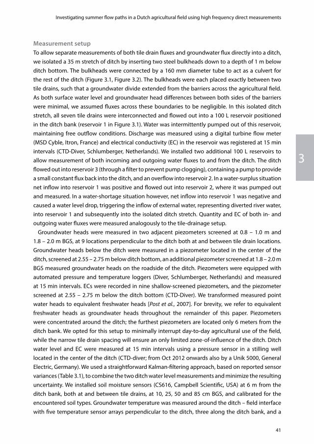
3

41


Measurement setupTo allow separate measurements of both tile drain fluxes and groundwater flux directly into a ditch, we isolated a 35 m stretch of ditch by inserting two steel bulkheads down to a depth of 1 m below ditch bottom. The bulkheads were connected by a 160 mm diameter tube to act as a culvert for the rest of the ditch (Figure 3.1, Figure 3.2). The bulkheads were each placed exactly between two tile drains, such that a groundwater divide extended from the barriers across the agricultural field. As both surface water level and groundwater head differences between both sides of the barriers were minimal, we assumed fluxes across these boundaries to be negligible. In this isolated ditch stretch, all seven tile drains were interconnected and flowed out into a 100 L reservoir positioned in the ditch bank (reservoir 1 in Figure 3.1). Water was intermittently pumped out of this reservoir, maintaining free outflow conditions. Discharge was measured using a digital turbine flow meter (MSD Cyble, Itron, France) and electrical conductivity (EC) in the reservoir was registered at 15 min intervals (CTD-Diver, Schlumberger, Netherlands). We installed two additional 100 L reservoirs to allow measurement of both incoming and outgoing water fluxes to and from the ditch. The ditch flowed out into reservoir 3 (through a filter to prevent pump clogging), containing a pump to provide a small constant flux back into the ditch, and an overflow into reservoir 2. In a water-surplus situation net inflow into reservoir 1 was positive and flowed out into reservoir 2, where it was pumped out and measured. In a water-shortage situation however, net inflow into reservoir 1 was negative and caused a water level drop, triggering the inflow of external water, representing diverted river water, into reservoir 1 and subsequently into the isolated ditch stretch. Quantity and EC of both in- and outgoing water fluxes were measured analogously to the tile-drainage setup. Groundwater heads were measured in two adjacent piezometers screened at 0.8 – 1.0 m and 1.8 – 2.0 m BGS, at 9 locations perpendicular to the ditch both at and between tile drain locations. Groundwater heads below the ditch were measured in a piezometer located in the center of the ditch, screened at 2.55 – 2.75 m below ditch bottom, an additional piezometer screened at 1.8 – 2.0 m BGS measured groundwater heads on the roadside of the ditch. Piezometers were equipped with automated pressure and temperature loggers (Diver, Schlumberger, Netherlands) and measured at 15 min intervals. ECs were recorded in nine shallow-screened piezometers, and the piezometer screened at 2.55 – 2.75 m below the ditch bottom (CTD-Diver). We transformed measured point water heads to equivalent freshwater heads [Post et al., 2007]. For brevity, we refer to equivalent freshwater heads as groundwater heads throughout the remainder of this paper. Piezometers were concentrated around the ditch; the furthest piezometers are located only 6 meters from the ditch bank. We opted for this setup to minimally interrupt day-to-day agricultural use of the field, while the narrow tile drain spacing will ensure an only limited zone-of-influence of the ditch. Ditch water level and EC were measured at 15 min intervals using a pressure sensor in a stilling well located in the center of the ditch (CTD-diver; from Oct 2012 onwards also by a Unik 5000, General Electric, Germany). We used a straightforward Kalman-filtering approach, based on reported sensor variances (Table 3.1), to combine the two ditch water level measurements and minimize the resulting uncertainty. We installed soil moisture sensors (CS616, Campbell Scientific, USA) at 6 m from the ditch bank, both at and between tile drains, at 10, 25, 50 and 85 cm BGS, and calibrated for the encountered soil types. Groundwater temperature was measured around the ditch – field interface with five temperature sensor arrays perpendicular to the ditch, three along the ditch bank, and a

42

Chapter 3

further one placed horizontally in the ditch along its bank. These arrays each consisted of a 4 m PVC rod containing 10 thermistors (S-THB, Onset, USA) located at 35 cm intervals from the bottom end. Ditch evaporation was measured using a floating evaporation pan, equipped with pressure sensors (Unik 5000, General Electric and 176PC, Honeywell, USA). Missing periods were filled using a fitted linear correction to calculated Penman evaporation values. Meteorological data were obtained from a meteorological station located on the south-eastern end of the field, consisting of a tipping bucket rain gage (ARG-100, Env. Systems, UK), solar radiation (SKS 1110 pyranometer, Skye Instr., UK), air humidity and temperature (HMP35, Vaisala, Finland), barometric pressure (VU Amsterdam, Netherlands), wind speed (A100R, Vector Instr., UK) and direction (W200P, Vector Instr., UK), and soil heat flux via thermocouple soil temperature measurements at 0.1 and 0.2 m depths. Crop condition and growth stage were inspected visually on a weekly basis. We measured soil hydraulic properties using both falling-head permeameter tests (Eijkelkamp, Netherlands) on core samples at different depths, and slug-tests [Beers, 1983] in existing piezometers. Continuous vertical electrical soundings (CVES; ABEM Terrameter SAS 4000, Sweden) with 0.5 m electrode spacings was performed on 29 March, 2012 and electromagnetic induction measurements were performed every 0.2 m in transects parallel to and perpendicular to the ditch on 11 February, 2014 (DUALEM 421, Dualem, Canada), to assess groundwater salinity distribution.

floating evaporation pan

meteostation: precip, temp, wind and radiation

array of temperature sensors perpendicular to ditch - field interface (not on photo)

instream reservoirs:measurement of Q and ECof drains, ditch and intake

7 tile drains connectedto instream reservoir

piezometers (1, 2 m BGS)at and between tile drains

culvert

soil moisture sensors;at and between tile drains

Figure 3.2 | Measurement setup.

3

43


Measurement periods were from 30 May 2012 to 1 Dec 2012 and from 15 Apr 2013 to 1 Oct 2013. The measurement setup was partly dismantled in the intermediate period to allow field cultivation. Estimated measurement uncertainty of measured parameters and measurement devices is listed in Table 3.1. All ECs were converted to Total Dissolved Solids (TDS) using an EC-TDS relation derived specifically for the coastal region of the Netherlands [Stuyfzand, 2014], its applicability was checked using 26 available local chemical analyses (Appendix 1). To comprehensively investigate flow routes to the ditch, we subsequently: (1) established the hydrological response of the field to the prevailing meteorological conditions, (2) investigated groundwater salinity and the salinity dynamics in exfiltration to tile drains and the ditch, and the resulting surface water salinity response, (3) separated flow route contributions to exfiltration fluxes, (4) quantified the exfiltration flux response to groundwater level variations, and (5) investigated the hydrological and solute response of the field to both a wet and a dry period in more detail.

Table 3.1 | Estimated measurement uncertainty for measured parameters.

Parameter Device Estimated uncertainty a Source

Groundwater head Schlumberger Diver ± 0.002 m [Schlumberger, 2010]

Ditch water level Schlumberger Diver ± 0.02 mb [Von Asmuth, 2010]

Ditch water level GE Unik 5000 ± 0.002 m [General Electric, 2012]

Discharge Itron propeller flow meter ± 1.5%c [Barfuss et al., 2011]

Evap pan water level GE Unik 5000 ± .002 m [General Electric, 2012]

Evap pan water level Honeywell 176PC ± .002 m [Honeywell, 2012]

Groundwater EC25 Schlumberger CTD-Diver ± 1.0%c [Schlumberger, 2010]

Gw temperature Onset S-THB ± 0.2 °C [Onset, 2013]

Soil moisture Campbell Sci CS616 ± 2.5%VWC [Campbell Sci, 2011]

Precipitation EML ARG-100 ± 0.1 mm [EML, 2009]

Solar radiation Skye Instr. SKS 1110 ± 5.0% c [Skye Instr., 2009]

Air humidity Vaisala HMP-35 ± 2.0% c [Vaisala, 1998]

Air temperature Vaisala HMP-35 ± 0.1 °C [Vaisala, 1998]

Barometric pressure VU Amsterdam ± 1 hPa VU, pers. comm.

Hydraulic conductivity Eijkelkamp permeameter ± 130% c Measurement repetition

Hydraulic conductivity Slug tests ± 35% c Measurement repetition

a Uncertainty is reported as 2 * standard deviation, unless stated otherwiseb Higher than groundwater head due to larger temperature differencesc 2 * relative standard deviation

Groundwater – surface water interactionUnlike the exfiltration of groundwater via the tile drains, the direct flow of groundwater into and from the ditch could not be measured. We therefore deduced the transient surface water – groundwater (SW-GW) interaction in the ditch by simultaneously solving the water, salinity, and heat balance of the ditch [e.g., Assouline, 1993; Martínez-Alvarez et al., 2011; Xing et al., 2012]. The simultaneous

44

Chapter 3

solution constrains uncertainty and allows for separation between the shallow and deeper flow paths to the ditch.

The water balance of the ditch can be written as:

qgw = qout – qin – qpr + qe + ΔV, (3.1)

with qgw denoting the SW-GW flux, qout the measured ditch outflow, qin the measured ditch intake flux, qpr direct precipitation, qe evaporation and ΔV the change in ditch volume (all in m3, schematic overview in Figure 3.3). Note that Eq. 3.1 excludes the contribution of tile drains, as they are kept completely separate from the ditch. All parameters of Eq. 3.1 are measured quantities, except the SW-GW flux. Analogously, the salinity balance can be written as:

qgw Cgw = qout Cout – qin Cin + ΔS, (3.2)

with Ci denoting the TDS (in g/L) of the various fluxes qi , and ΔS the change in TDS storage (kg). Note that Cgw is the (unknown) flux-weighted mean TDS of exfiltrating groundwater, and that TDS of precipitation and evaporation are assumed zero (acceptable given the large TDS contrast between groundwater and precipitation). Finally, the heat balance, including terms for incoming radiation and sensible and latent heat loss but ignoring kinetic processes, reads [Anderson, 1952]:

1qgwTgw = qoutTout – qinTin – qpr + Teqe + { ρwλ(1 + β)qe – A(Rn – G)} + ΔHcv

, (3.3)

with Ti denoting the temperature (K) of the various fluxes qi, cv the volumetric heat capacity of water (MJ/m3K), rw water density (kg/m3), λ the latent heat of vaporization (MJ/kg), β the Bowen ratio (-), A the ditch area (m2), Rn the net radiation (MJ/m2), G conduction through the ditch bottom (MJ/m2), and ∆H the change in heat storage (m3K). We calculated Rn from the available weather data using the standardized calculation procedure outlined in [Allen et al., 1998; Valiantzas, 2006], and β according to Bowen (1926). While generally neglected because of its small magnitude [Anderson, 1952; Assouline, 1993], we included the conduction of heat through the ditch bottom G in the balance equation, as we expect the influence to be uncharacteristically large due to the large perimeter-volume-ratio. G becomes especially important when solving Eq. 3.3 on hourly time steps. Analogous to Eq. 3.2, Tgw is the (unknown) flux-weighted mean temperature of exfiltrating groundwater.

Denoting the known right hand sides of Eqs. 3.1 – 3.3 as W, S, and H, the system of equations can be written in matrix form as:

1

gw gw

gw

WC q ST H

=

, (3.4)

3

45


three linear equations with three unknowns: qgw, Cgw and Tgw. Given these three unknowns, the system is well-determined, and the simultaneous solution has no purpose in constraining the uncertainty in qgw. We therefore assumed the exfiltrating groundwater to be a conservative mixture of shallow (exfiltrating along the ditch edge) and deeper groundwater (exfiltrating in the centre of the ditch), of which we have measured both the EC (converted to TDS) and temperature (see coloured lines in Figure 3.3). By adding this extra information, Eq. 3.4 becomes the over-determined system:

,, ,d

,, ,

1 1gw s

gw s gwgw d

gw s gw d

Wq

C C Sq

T T H

=

, (3.5)

with the subscripts gw,s and gw,d denoting shallow and deep groundwater flow paths respectively. So far, we only discussed the exfiltration situation. When infiltrating however, TDS and temperature of the infiltrating groundwater change to the TDS and temperature of the ditch, yielding the following nonlinear system of equations (note that the shallow and deep groundwater flux can no longer be distinguished in the infiltration situation):

, when qgw>0

1 1Cgw,s Cgw,dTgw,s Tgw,d

1 1Cditch CditchTditch Tditch

WSH

WSH

qgw,sqgw,d

qgw,sqgw,d

=

, when qgw<0=

(3.6)

We solved this nonlinear system, with the added constraint that the sign of qgw,s should equal that of qgw,d, using Sequential Least Squares Programming [Kraft, 1988] to minimize the sum of squares weighted by the inverse of right-hand-side variances. The additional constraint proved necessary to prevent fits with large opposite values of qgw,s and qgw,d. In addition, we applied a Monte Carlo analysis (n=1000) to Eq. 3.6, randomly sampling Gaussian distributions around all measured parameters (using measurement variances reported in Table 3.1), to quantify the uncertainty in the calculated values of qgw. Throughout the remainder of this paper, we refer to the (calculated) direct flow of groundwater into and from the ditch as ditch exfiltration and ditch infiltration respectively, and to the (measured) exfiltration of groundwater into the tile drains as drain exfiltration. The measured discharge of the ditch, the non-separated result of different flow routes, is referred to as ditch discharge.

46

Chapter 3

Figure 3.3 | Schematic overview of fluxes (qpr precipitation, qe evaporation, qin ditch intake flux, qout ditch discharge, qgw groundwater in- / exfiltration) entering and exiting the ditch (black lines). Coloured lines represent the separation of qgw in a shallow (qgw,s) and a deep (qgw,d) component, and measurement locations of C (concentration, TDS) and T (temperature) of these fluxes; ΔV is volume change of ditch water.

RESULTS

water fluxesThe two measurement periods differed markedly in their meteorological conditions. The months of June to August 2012 were relatively wet (recurrence interval of the cumulative precipitation deficit 1.3 y, derived from a Gumbel distribution fitted to 50+ years of weather records of the nearby De Kooy meteorological station). The same period in 2013 was relatively dry (recurrence interval 14 y). These conditions were reflected in the measured hydrology of the field site (Figure 3.4, Table 3.2). Measured precipitation averaged 2.89 mm/d in 2012 (long-term average 2.45 mm/d for this period), while precipitation was limited to an average of 2.11 mm/d in 2013, including the wet period from 10 September 2013 onwards. Potential evapotranspiration, calculated according to the FAO Penman-Monteith method [Allen et al., 1998] and accounting for observed crop growth, amounted to 2.95 mm/d and 2.48 mm/d respectively. We assumed actual transpiration to match potential transpiration throughout the measurement period, due to the excellent water retention characteristics of the soil and used shallow soil moisture measurements to correct bare soil evaporation [Allen et al., 1998]. Excess water is discharged from the field by exfiltration to both tile drains and ditches. Drain exfiltration was significantly higher than ditch exfiltration and averaged around 1.1 mm/d (2012) and 0.9 mm/d (2013). Ditch ex- /infiltration amounted to 0.1 mm/d of exfiltration in 2012, equal ditch infiltration and exfiltration fluxes of 0.2 mm/d added up to a net 0 mm/d in 2013 (note that all mm are areal averages over the entire field-plus-ditch area, unless stated otherwise). Closure of the water balance required between 1.2 mm/d (2012) and 0.9 mm/d (2013) of additional influx of water, mainly representing the influx of regional groundwater flow (Table 3.2).

3

47


Figure 3.4 | Precipitation and evapotranspiration (mm/d) (a), volumetric water content soil (-) (b), ground- and surface water level (m BGS) (c) and discharge (mm/d) (d) during measurement periods. Missing data are due to system malfunction (filter clogging, power failure).

48

Chapter 3

Table 3.2 | Water balance field site.

Parameter June – Sept 2012a June – Sept 2013

mm/d % mm/d %

Precipitation 2.89 70.4% 2.11 57.9%

Sprinkler irrigationb 0.00 0.0% 0.41 11.1%

Ditch infiltrationc 0.01 0.2% 0.19 5.3%

Total in 2.90 70.5% 2.71 74.3%

Evapotranspiration 2.95 71.7% 2.48 67.9%

Tile drain exfiltration 1.06 25.7% 0.94 25.7%

shallow flow pathc 0.80 19.5% 0.78 21.5%

deep flow path c 0.26 6.2% 0.15 4.2%

Ditch exfiltrationc 0.09 2.2% 0.19 5.2%

shallow flow path c 0.05 1.1% 0.16 4.4%

deep flow path c 0.04 1.0% 0.03 0.8%

Storage change 0.01 0.3% 0.04 1.2%

Total out 4.11 100.0% 3.65 100.0%

Closure 1.21 29.5% 0.94 25.7%

(Flushing demand) c,d 4.93 117.5% 2.36 64.5%

a Limited to the period 15 June – 23 September due to system malfunctionb Estimated irrigation amount of 25 mm per event c Based on calculation rather than direct measurement d Based on norm TDS of 1.5 g/L and intake water TDS of 0.7 g/L

Measured groundwater levels reflect the varying meteorological conditions during the two measurement periods (Figure 3.4c). A succession of precipitation events throughout the 2012 measurement period resulted in rapidly changing groundwater levels, which remained above drain depth throughout the measurement period. Groundwater levels remained below the ground surface, peaking at 0.55 m BGS. Drier conditions in 2013 resulted in much less variation in groundwater levels between May and July 2013, after which groundwater levels dropped significantly below drainage depth and eventually ditch bottom, reaching a maximum depth of 1.65 m BGS. The dry period in 2013 prompted the farmer to irrigate the growing lettuce on two accounts (11 and 16 July 2013), leading to only small increases in soil moisture, and no noticeable effect on groundwater levels. Sprinkling water was obtained from the (not-instrumented) ditch bordering the field on its southern side. A large precipitation event on September 10 ended the long dry period and caused groundwater levels to quickly rise to a maximum of 0.7 m BGS. The measurement and control setup aimed to keep the ditch water level at a level of 1.12 m BGS, just below drainage depth, and as constant as possible. However, the abundance of suspended fine-grained particulate and organic matter in the ditch caused filter clogging, which was a recurring issue before a redesign of the ditch filter on October 26, 2012. Large ditch water level variations between September 23 and October 26, 2012, were due to a rupture in the ditch culvert caused by

3

49


mowing activities. Periods experiencing filter clogging, significant water level variations or power failures were discarded from further analyses. We were able to separately measure both ditch discharge and intake and tile drain discharge in 15 minute increments for most of the measurement periods. All measurements were averaged to hourly periods for subsequent analyses. Tile drain discharge was on average 1.3 mm/d and varied between zero and 11.5 mm/d, showing a similar pattern to those of the observed groundwater levels. In 2012, drain discharge was sustained throughout the summer period. Drain discharge however ceased during the months of July and August 2013 after groundwater levels dropped below drainage depth. Drain discharge exhibited the characteristic tailing after a peak that is consistent with drainage theory [De Zeeuw and Hellinga, 1958; Kraijenhoff van de Leur, 1958]. Ditch discharge was on average 0.2 mm/d and varied between -1.3 mm/d (intake) and 8.4 mm/d and was generally more gradual than tile drain discharge. An uncharacteristically large ditch discharge was recorded on September 10 2013, presumably due to a significant contribution of overland flow, caused by a large precipitation event (41 mm in 24 hours) following a prolonged dry period. Our measurement setup did not allow separating between overland flow and groundwater exfiltration.

Figure 3.5 | Measured and calculated open water evaporation values, in the instrumented ditch (a), and the wider and deeper ditch on the other side of the field (b). Solid lines denote the linear regression lines, dashed lines and shaded areas represent the 95% confidence interval of the regression and the 95% prediction interval respectively, the 1:1 line is indicated in dashed grey.

Ditch floating evaporation pan measurements were only available for 2012. To extend the evaporation time series to 2013, we correlated measured open water evaporation to evaporation calculated using the standard Penman formula [Penman, 1948; Valiantzas, 2006] (Figure 3.5). Measured values correlated well with calculated values, but were consistently lower, and appeared to require a minimum amount of radiation (Epan = 0.48EPenman – 0.73, RMSE 0.62 mm/d). Calibration of the ‘wind function’ could not improve the calculation. Rather, deviations between measured and calculated values were predominantly related to an apparent overestimation of (net) incoming

50

Chapter 3

radiation. We also operated a floating evaporation pan in the ditch on the southern end of the field. This ditch is both wider (3 m) and deeper (0.5 m) than the instrumented ditch. Penman evaporation estimates only slightly overestimated measured evaporation in this ditch (Epan = 0.84EPenman – 0.32, RMSE 0.93 mm/d). In all subsequent hourly analyses, we down-scaled daily evaporation values using hourly short-wave radiation measurements.

Figure 3.6 | TDS variation and contribution to salinity load to surface water, with (a) precipitation and evapotranspiration (mm/d), (b) TDS of tile drains, ditch and intake (g/L), (c) TDS load of tile drains, ditch and intake (kg/d), (d) fraction of tile drains, ditch and intake in TDS load (-), and (e) calculated TDS of ditch if non-separated (g/L) and required flushing flux to keep surface water TDS at 1.5 g/L (mm/d).

3

51


Groundwater and surface water salinityThe main origin of exfiltrating solutes at the field site is the upward flow of brackish regional groundwater, exfiltrating in tile drains and ditches. Converted measurements of groundwater salinity showed an average TDS at 2 m BGS of 13.0 (± 1.4) g/L, whereas groundwater TDS at 1 m BGS is on average 0.43 (± 0.24) g/L. Average TDS of the tile drain discharge over the measurement periods was 3.3 g/L, while the average TDS of ditch discharge was 7.7 g/L over this period, signifying a preferential flow of higher-salinity groundwater to the ditch (Figure 3.6). Both drain and ditch salinity decreased during and increased between discharge events. Even though salinity of ditch discharge was significantly higher than tile drain discharge, salinity loads towards the surface water are dominated by tile drainage. Tile drains transported about three times more solutes than ditch exfiltration. The relative contribution of the ditch in the solute load increases between precipitation events however, reaching over 80% in prolonged dry periods. Table 3.3 lists the salinity balance of the field site, showing a necessarily large closure term reflecting the inability to measure the regional groundwater input to the salinity balance.

Table 3.3 | TDS balance field site.

Parameter June – Sept 2012a June – Sept 2013

kg/d % kg/d %

Precipitationb 0.53 2.4% 0.39 2.7%

Fertilizer applicationc 0.24 1.1% 0.24 1.6%

Sprinkler irrigationd 0.00 0.0% 1.31 9.0%

Ditch infiltratione 0.40 1.8% 0.86 5.9%

Total in 1.17 5.3% 2.79 19.1%

Evapotranspirationf 0.25 1.1% 0.20 1.4%

Tile drain exfiltration 17.50 79.2% 11.89 81.5%

shallow flow pathe 1.94 8.8% 1.77 12.1%

deep flow pathe 15.56 70.4% 10.12 69.4%

Ditch exfiltratione 4.35 19.7% 2.49 17.1%

shallow flow pathe 1.11 5.0% 0.64 4.4%

deep flow pathe 3.23 14.6% 1.85 12.7%

Storage change ? ? ? ?

Total out 22.09 100.0% 14.58 100.0%

Closure 20.92 94.7% 11.79 80.9%

a Limited to the period 15 June – 23 September due to system malfunctionb Bulk TDS precipitation 48 mg/L [Stuyfzand, 1993]c Estimated at 100 kg/ha/j Cl [Eertwegh and Meinardi, 1999]d Estimated irrigation amount of 25 mm per event, TDS measurede Based on calculation rather than direct measurement f From estimated plant uptake concentration of 10 mg/L Cl [Van der Velde et al., 2010b]

52

Chapter 3

We determined the ditch surface water salinity that would have occurred without physical separation of flow routes by assuming complete mixing of the different flow paths entering the ditch with the resident ditch volume at each successive time step. In addition, we calculated the amount of flushing (assuming constant salinity of 0.7 g/L intake water) required to keep surface water TDS at 1.5 g/L , the local salinity norm for irrigating potatoes (Figure 3.6e). Unseparated ditch surface water salinity would have varied between about 3 to 7 g/L (excluding intake periods), both through salinity variations of drain and ditch exfiltration and through variation in the relative proportion of drain or ditch exfiltration in the ditch. Flushing demands vary significantly and may reach 25 mm/d (note that absolute amounts are conditional on the chosen salinity norm). The flushing demand was largely determined by the salt load entering the ditch and therefore reached peak values during discharge events, even though unflushed surface water salinity was then at its lowest. Calculated flushing demands were approximately equal to the sum of the other water balance components at the field site (Table 3.2).

15 m

50 m

0 10 20 30

resistivity [ Ωm]

road

instrumented ditch

ditch

agricultural �eld

0-1.2

6

b

a

CVES DUALEMinstrumentedditch

agricultural�eld

35m

125m

c

0

2

4

6

8-20 -15 -10 -5 0 5 10 15 20

dept

h [m

BG

S]

x-coordinate [m]

0 20 40 60

resistivity [ Ωm]tile drain

dept

h [m

BG

S]

Figure 3.7 | Resistivity profiles measured by CVES (a) and DUALEM (b), locations in (c). Note the different resistivity scale between (a) and (b).

3

53


Inversion results of CVES and DUALEM measurements (Figure 3.7), showed a clear pattern of brackish groundwater at very shallow depths (2 – 3 m BGS), overlain by fresher water. The CVES result has a much higher vertical resolution, and shows the upconing of brackish water towards the tile drains, located at 5 m intervals. An alternating pattern is visible in the upconing of brackish water to tile drains, likely related to the drains being alternately older and more recent, and could result from a lower drainage resistance of the newer tile drains [Velstra et al., 2013]. The DUALEM system is a Frequency Domain EM (inductive coupling) system and, because of limited antenna orientations, offered a lower resolution in the vertical than CVES. DUALEM was, however, easier to operate on transects perpendicular to the field, crossing two ditches and a busy agricultural road. The low vertical resolution caused the inversion (EM4Soil) to calculate unrealistic increasing resistivities at greater depths. DUALEM results revealed the limited zone of influence (10 m) of the ditch on the salinity distribution beneath the agricultural field. Within this zone of influence, brackish water cones up towards the ditch. However, the results also indicate a small pocket of fresher water beneath the ditch bottom, which seems to indicate mixing with fresher water coming from the ditch sides. DUALEM results beneath the elevated road should be interpreted with caution, as the inversion was unable to adequately match the measured conductivities at lower depths. Still, results exclude the presence of a significant freshwater lens underneath the elevated road, possibly related to limited infiltration from the road surface. Low conductivities just below the road compared to the field resulted from lithological differences (sand bed below the road) and a lower moisture content.

Flow path separationThe simultaneous solution of the water-, salinity, and heat-balance of the ditch enabled the calculation of direct groundwater flow to and from the ditch (Figure 3.8, daily time step), and we assessed the associated uncertainty with a Monte Carlo analysis. Judging from the small uncertainty bands, the total groundwater exfiltration in the ditch could be well-discerned. Application of Eq. 3.6 further allowed the separation of ditch exfiltration in shallow and deep flow paths, based on the varying measured contrasts in both TDS and temperature, again with Monte Carlo-derived uncertainty ranges. The contrast in TDS was large and relatively constant at about 8 g/L, temperature contrast averaged only 0.2 °C and was more variable. In addition, assuming a fixed TDS for both regional groundwater flow and meteoric water, we straightforwardly separated tile drain discharge in meteoric and regional groundwater origins. Varying TDS between minimum and maximum measured values (12 – 17 g/L and 0 – 0.7 g/L for deep groundwater and meteoric water respectively) hardly affected the separation result, as demonstrated by the narrow uncertainty range surrounding the regional flow contribution to drain exfiltration. Note that the separations of ditch and tile drain exfiltration are not directly comparable, as the shallow flow path to the ditch in particular is itself a mixture of meteoric and regional groundwater.

54

Chapter 3

Figure 3.8 | Flow path separation of drain and ditch exfiltration, with precipitation and evapotranspiration (mm/d) (a), drain exfiltration and deep groundwater contribution to drains (mm/d) (b) and ditch ex- and infiltration and deep flow path contribution (mm/d) (c). Missing data periods are caused by power failures or filter clogging. (Thin) shaded area in (b) around the deep groundwater contribution is based on min – max values for both deep groundwater and rainwater TDS, shaded areas in (c) span the Monte Carlo 25 – 75 percentile values, lines denote the median values.

Groundwater interaction with the ditch varied from a maximum infiltration rate of 1.4 mm/d, to a maximum exfiltration of 8.6 mm/d. These values were both slightly higher than the corresponding ditch intake / discharge, due to storage effects in the ditch and, to a lesser extent, to the contribution of precipitation and evaporation to the ditch water balance. The separation showed a consistently high contribution of deep regional groundwater to ditch exfiltration compared to drain exfiltration, in accordance with the measured salinity loads of the ditch. After the infiltration period in Aug 2013 however, the contribution of regional groundwater flow in ditch exfiltration was nearly zero. Groundwater that exfiltrated in the ditch during the subsequent precipitation event likely consisted primarily of water that infiltrated during the preceding period was attributed to the shallow flow path on account of its low salinity. The small peak in regional groundwater contribution just after the infiltration period probably resulted from water still stored in the collector reservoir from before the infiltration period. Excluding the peak possibly caused by overland flow, only 15 mm exfiltrated between Sep 10 and Oct 1, while a total of 29 mm infiltrated during the preceding period.

3

55


Hooghoudt drainage modelWe analysed drain exfiltration (measured) and ditch exfiltration (calculated) versus measured head difference (Figure 3.9), which revealed a clear difference between the two. While the relation was approximately linear for ditch exfiltration, drain exfiltration showed a much steeper and about exponential increase of exfiltration with increasing head difference. The steeper incline of drain exfiltration is a logical result of the lower resistance to flow to the tile drains. The exponential shape indicates a decrease in drainage resistance when groundwater levels rise. The lowering of the resistance to drainage when groundwater levels rise and the flow area increases is well-known in drainage theory, when the rise is significant relative to the total flow area [e.g., Hooghoudt, 1940; Ernst, 1962]. This is represented by the second, quadratic term in the classic Hooghoudt equation [Hooghoudt, 1940]:

8k2De�m0 + 4k1m02, if m0 ≥0

L2

q

=

8k2De�m0 – 4k1m02

L2, if m0 <0

, (3.7)

in which q is specific discharge (m/d), k1 and k2 are the hydraulic conductivity above and below the drainage level respectively (m/d), Deff is the effective depth of flow (the total flow depth corrected to account for radial flow, calculated using [Moody, 1966], m0 is the difference between the groundwater level at 0.5L and the ditch water level. Judging from fitting Eq. 3.7 to the data with a single hydraulic conductivity (12 cm/d), this phenomenon alone is not enough to explain the curvature apparent in Figure 3.9. A better approximation of the curvature in the drain data required a higher hydraulic conductivity above (k1 = 50 cm/d) than below (k2 = 1 cm/d) the drain depth (Figure 3.9).

Figure 3.9 | Discharge versus head difference for drain exfiltration and ditch ex-/infiltration. Dashed lines are Hooghoudt equations (Eq. 3.7) fitted to the data with denoted hydraulic conductivities.

56

Chapter 3

The linear relation of ditch exfiltration indicates a negligible influence of head variations on the drainage resistance, pointing towards a significantly deeper flow system compared to the drains (first term in Eq. 3.7 >> second term). Flow towards the ditch could be well approximated applying Eq. 3.7 both for the southern (field) and northern side of the ditch, using a single hydraulic conductivity of 5 cm/d. Slug test-measured hydraulic conductivities ranged from 0.5 to 6 cm/d, whereas falling-head permeameter results of loamy-sand samples ranged from 2 to 6 cm/d (clayey top layer samples ranged from 0.001 to 0.3 cm/d (average 0.07 cm/d). Fitted hydraulic conductivities correspond well to measured values, especially for the linear domain. The slug tests were performed during a relatively dry period, when groundwater levels were only about 10 cm above drainage depth, so possibly could not capture a higher hydraulic conductivity at shallower depths. Note that drain exfiltration appeared to be maximized at about 0.7 mm/h, likely caused by the installed maximum pumping capacity (Figure 3.9). The ditch exfiltration values that exceed 0.7 mm/h, at a head difference of only 0.2 m, all occurred during the ditch discharge peak following the infiltration period of Aug 2013.

Individual eventsPrecipitation eventWe took a closer look at the variation of drain and ditch exfiltration and their composition during a representative precipitation event that started October 29, 2012 (Figure 3.10). We therefore separated flow paths by applying Eq. 3.6 on an hourly instead of a daily time step. Uncertainty in calculated hourly ditch exfiltration proved to be relatively larger than uncertainty on a daily time step, predominantly due to the increased importance of (the uncertainty in) the storage terms in the hourly balance (Eq. 3.6). Nevertheless, the exfiltration process towards the ditch could be well identified. Drain discharge lagged five hours behind the onset of precipitation, closely following the groundwater level response in the field, and again displayed the characteristic tailing-after-peak. The separation of drain exfiltration in shallow flow of local meteoric origin, and deep regional groundwater flow showed the preferential discharge of meteoric water during the discharge peak. TDS of drain exfiltration therefore decreased from 4.8 to 2.2 g/L. Still, the total salt flux exfiltrating via the tile drains increased, as the precipitation event also triggered a rise of the brackish deep flow component. Direct groundwater exfiltration to the ditch showed a similar pattern to drain exfiltration, albeit at a roughly seven times lower rate. Ditch exfiltration reacted faster and persisted longer compared to exfiltration to tile drains, corresponding with the observed pattern in groundwater head below and alongside (not shown) the ditch. The separation between shallow and deeper flow paths revealed a quick response of deeper groundwater, while the contribution of shallower flow paths lagged by about 12 hours. A similar pattern was observed for other events.

3

57


Figure 3.10 | Precipitation event Oct 29 2012, with (a) precipitation and evapotranspiration (mm/d), (b) groundwater and ditch surface water levels during the event (m BGS), (c) TDS of drain and ditch exfiltration (g/L), (d) total exfiltration and contribution of deep groundwater to tile drains (mm/d), (e) total exfiltration and contribution of deep groundwater to ditch (mm/d) and (f) fraction of deep groundwater in drain and ditch exfiltration. Shaded areas denote 25th and 75th percentile of Monte Carlo runs. Note that fluxes are in mm/d for consistency, but all data are hourly values.

58

Chapter 3

Figure 3.11 | Infiltration event Jul – Aug 2013, with (a) precipitation (mm/d), evapotranspiration (mm/d) and ditch water temperature (°C, secondary y-axis), (b) groundwater and ditch surface water levels (m BGS), (c) ex- / infiltration to and from ditch, intake flux and drain exfiltration (mm/d), and (d) ditch water temperature, groundwater head ditch and ditch infiltration between Aug 4 and Aug 6. Ditch ran dry from Jul 14 to Jul 31. Shaded area around ditch ex- / infiltration denotes 25th and 75th percentile of Monte Carlo runs. Note that fluxes are in mm/d for consistency, but all data are hourly values.

3

59


Infiltration eventConditions were dry throughout July and August, 2013, causing a gradual decline in groundwater heads, to a maximum 5.6 m BSL (1.6 m BGS) (Figure 3.11). Exfiltration via the drains stopped on July 8 and exfiltration to the ditch switched to an infiltration situation quickly after. Infiltration was short-lived, as the ditch ran dry due to a mechanical failure in the intake system. This dry period lasted until July 31, when the intake possibility was restored. After an initial intake peak to restore the determined ditch water level, infiltration continued to follow the variation in head difference between surface and groundwater. Groundwater heads suddenly rose 8 and 7 cm below the ditch and in the field, respectively, within hours after intake was restored, showing no signs of a disconnect between ditch and groundwater. Groundwater heads subsequently continued their decline, but began to rise after 10 days of infiltration. Deviations from this pattern on August 14 and 15 are most likely only an artefact of combining hourly water level fluctuations with an only cumulatively known intake flux for that period (logger power failure). Preferential flow of the fluctuating ditch water to the then-submerged tile drains is the likely cause of the intermittent small tile drain exfiltration in August. The lettuce crop was harvested on August 9 2013 and the field was tillaged on August 12. At about the same time, heads started to rise from 1.55 m BGS to a relatively stationary level of 1.2 m BGS that was reached on August 23. Groundwater heads both below the ditch, next to the ditch (not shown) and in the field showed a similar pattern. Whereas groundwater levels fell before harvesting as precipitation, upward regional groundwater flow and sideways infiltration from the ditch could not compensate for crop transpiration, groundwater levels recovered after harvesting. This is likely the result of a sharp decrease in evapotranspiration, as bare soil evaporation (corrected using shallow soil moisture measurements [Allen et al., 1998] amounted to about 1 mm/d versus 3 mm/d if the crop had remained on the field. Infiltration abruptly ended September 10, when 40 mm of precipitation resulted in a groundwater rise of 80 cm and both tile drain and ditch exfiltration were restored. Net infiltration over the preceding period totalled 27 mm, while only 0.4 mm (1.5%) of ditch intake water was lost to evaporation. Note again that these values are areal averages over the entire field-plus-ditch area. Depending on the estimated storage difference of between 8 and 19 mm (16 cm head difference, assuming a specific yield between 0.05 and 0.12; literature range for the soil type considered [Wösten et al., 2013]), closure of the water balance during the infiltration period required between 0.5 to 1 mm/d of regional groundwater flow. We observed diurnal patterns in the observed infiltration rates (Figure 3.11d), as well as in exfiltration rates during low-flow periods (not shown). The diurnal patterns were correlated to both ditch temperature variations, and diurnal patterns in groundwater heads. The amplitude of the infiltration variations, superimposed on the general trend of increasing infiltration rates, was 0.12 mm/d, or 10% of the concurrent infiltration rate. The concurrent 3 °C amplitude temperature variations could result in an 8 % variation in hydraulic conductivity [Muskat, 1937; Constantz et al., 1994]. The amplitude of diurnal patterns in groundwater head, attributable to diurnal patterns in evapotranspiration in the field, was 2 cm, or 5% of the total head difference between surface water and groundwater.

60

Chapter 3

DISCUSSIoN

We instrumented an agricultural field to physically separate and measure the different flow paths contributing to the water and salinity balance of a headwater ditch, and specifically focused on agriculturally important summer periods. The on-going agricultural use of the field site proved challenging: our study suffered on several occasions from data loss due to filter clogging, power and mechanical failures. Nevertheless, we were able to continuously measure tile drain outflow and both ditch outflow and intake for the majority of the meteorologically different 2012 and 2013 growing seasons. While direct measurement of groundwater exfiltration in the ditch was impossible, the simultaneous solution of the water, salinity and heat balance of the ditch enabled the quantification of ex- and infiltration of groundwater to and from the ditch. Although presumably an underestimation due to the inability to include epistemic, non-random errors in our analysis [Beven, 2006a], Monte Carlo analysis indicated acceptable uncertainty in the exfiltration quantification. Upward flow of brackish regional groundwater at the field site resulted in a significant salinity contrast with infiltrating precipitation water. This contrast provided a unique opportunity to discern the different groundwater flow routes towards tile drains and the ditch and allowed for the mapping of the subsurface distribution of the two water types using geophysics. We observed groundwater levels in the field to react within hours to precipitation events, even after prolonged dry periods, signifying only minor influence of the shallow unsaturated zone on the timing of discharge events. The response of tile drain and ditch exfiltration to groundwater levels could be satisfactorily characterized using conventional drainage theory [Hooghoudt, 1940], using hydraulic conductivities comparable to values measured in the field. Tile drains were fed by a shallow flow system. Drains responded nonlinearly to groundwater level variations, attributable to nonlinearity in drainage resistance and a possible increase in hydraulic conductivity upwards in the soil profile. Higher hydraulic conductivities near the ground surface have been frequently observed and linked to the presence of macropores in the soil [Beven and Germann, 1982, 2013; Tiktak et al., 2012]. In contrast, groundwater flows to and from the ditch were linearly related to head differences, indicating a deep flow system and negligible influence of groundwater level variations on drainage resistance. Alternatively, anisotropy could also be a factor in explaining the observed differences in apparent hydraulic conductivity between the shallow, strongly radial flow to tile drains and the deeper flow paths to the ditch [Smedema et al., 1985]. Our results showed no evidence for differences in resistance between exfiltration and infiltration that have been observed in other settings and attributed to clogging processes [Blaschke et al., 2003; Cox et al., 2007; Doppler et al., 2007]. Ditch in- and exfiltration rates showed diurnal patterns that likely resulted from both the temperature-dependence of hydraulic conductivity [Muskat, 1937; Constantz et al., 1994] and evapotranspiration-induced diurnal head variations. Geophysical measurements disclosed the presence of brackish groundwater, originating from regional groundwater flow, within two m BGS. Brackish groundwater showed previously reported [De Louw et al., 2011b, 2013b; Velstra et al., 2011] upconing patterns towards the tile drains, while measurements indicated the exfiltration of brackish groundwater along the entire wet perimeter of the ditch. Consequently, salinity of ditch exfiltration was significantly higher than tile drain exfiltration (TDS of 11 and 3.6 g/L respectively, excluding the post-infiltration period, when the

3

61


exfiltration to the ditch consisted of previously infiltrated intake water). Salts were transported to surface water in a complex, time-varying pattern. While tile drainage was the dominant source of salt input in to surface water during the study period (80%, Table 3.3), the composition of salt origin was highly variable. Tile drains dominated the salt load during discharge events, but 80% of the ditch water composition during drier periods originated from ditch exfiltration (Figure 3.6). During discharge events, tile drain salinity decreased by about 50%, pointing to a larger proportion of discharge originating from shallow flow paths delivering freshwater to the tile drains. This pattern corresponds to previous observations in similar settings [Velstra et al., 2011; De Louw et al., 2013b]. Ditch exfiltration salinity on the other hand first increased, then decreased over the course of discharge events, concurrent with the observed responses of the shallow and deep flow paths to the ditch. While the observed pattern in tile drain salinity has been attributed to preferential flow of meteoric water via macropores [Velstra et al., 2011; De Louw et al., 2013b], such a mechanism would not explain the observed initial rise in ditch exfiltration salinity. We conceptualize the different timings of water with shallow and deep signatures to arise from the difference between pressure wave celerity and water velocity. Pressure is quickly propagated through the subsurface and flow directions change accordingly when groundwater levels rise. However, the salinity distribution lags behind, as it requires the actual flow of groundwater to change the salinity distribution. This difference results in the preferential exfiltration of groundwater with a deep flow path signature, as this groundwater type is initially also exfiltrated by shallow flow paths (Figure 3.12b, shallow flow paths intersecting lagging saline deep groundwater type). Water with a shallow flow path signature only reaches the ditch when the dynamic equilibrium between flow direction and salinity distribution is restored, thereby decreasing exfiltration salinity (Figure 3.12c). Quantifying the timing of deep and shallow flow path response may therefore prove useful in inferring subsurface properties (e.g., effective porosity), but was outside the scope of this research. Standard water management practice of polders in the Netherlands supports their mainly agricultural use and entails diverting fresh river water to supplement summer precipitation deficits and dilute surface water salinity levels using a more or less constant flushing regime to enable sprinkling irrigation. Surface water demands of the field site averaged over the dry growing season of 2013 were largest for flushing (2.4 mm/d; calculated value), then sprinkling irrigation (0.4 mm/d), and finally groundwater infiltration (0.2 mm/d), while open water evaporation was negligible. Combined demands to enable sprinkling irrigation were therefore over six times the irrigation amount in the 2013 growing season. Despite the large upward flow of regional groundwater in the studied polder, we found ditch infiltration to constitute a significant loss of diverted river water, amounting to a maximum of 1.5 mm/d over the catchment area (188 mm/d per ditch length unit). Low evaporation from the ditch resulted in evaporation accounting for only 1.5% of intake loss during the infiltration period (the remainder lost to infiltration). Evaporation from the instrumented ditch was, however, poorly estimated using the routinely applied Penman formula, which overestimated ditch evaporation by a factor of two. Evaporation measurements from a different ditch revealed large differences in evaporation rates between ditches; further study is necessary to unravel the specific processes steering evaporation from small ditches and better predict ditch evaporation. Calculated flushing demands varied widely over time, controlled by the salt load entering the ditch; demands were high during wet periods and low during dry periods. As sprinkling irrigation is only

62

Chapter 3

applied during dry periods, this result could imply significant water savings when flushing is either operationally controlled, dependent on salinity levels and sprinkling needs, or set to a constant flux calibrated to accommodate only dry periods.

Before rainfallFlow and salinity distribution in dynamic equilibrium

Shortly after rainfallGroundwater levels rise: ow responds quickly, discharge increasesSalinity distribution response lags: 'shallow' owpaths discharge 'deep' groundwater, exempli�ed by owpath intersecting concentration boundary, denoted by red circle

After some timeSalinity distribution again in equilibrium with owdistribution: 'shallow' groundwater ex�ltrates

a

b

c

Figure 3.12 | Conceptual representation of timing of shallow and deep exfiltration to ditch. Dotted lines depict the flow path distribution, thick arrows the movement of the fresh-saline interface. Note that the drawn sharp interface is in fact a continuum between fresh and saline groundwater [De Louw et al., 2013b], and timescales of discharge events are too short to reach equilibrium conditions. Red circle in (b) denotes ‘shallow’ flow path intersecting concentration boundary, thereby transporting ‘deep’ groundwater.

We did not specifically address density effects in our analyses, other than correcting head measurements. However, Simmons (2005) argued the importance of including density effects when studying groundwater flow, even when only small concentration gradients exist, by equating a typical head gradient of 10-3 to the density effect caused by a density difference of 1 kg/m3 (5% seawater). In an agricultural setting similar to our field site, with head gradients in the order of 10-1 m, [De Louw et al., 2011b] found negligible influence of variable-density flow. Head gradients in the Schermer polder field site are also in the order of 10-1 m, while density differences are maximum 8 kg/m3 [Post, 2012], suggesting only minor influence of density effects on groundwater flow. Still, density could be an important factor in drier periods, when head gradients are smaller. For instance, density could influence the infiltration rate induced by a head gradient of 0.025 (August 23 – September 5, 2013) by over 30 %. We aim to further address the influence of density differences in further work.

3

63


CoNCLUSIoN

This study presents results of high frequency measurements of groundwater – surface water interaction in an instrumented agricultural field in a deep polder in the coastal region of the Netherlands. Simultaneous measurements of discharge, electrical conductivity and temperature allowed the separation and investigation of flow paths transporting water and salts to surface water, and disclosed complex and time-varying patterns of tile drain and ditch exfiltrationDespite their lower salinity, tile drains transported the majority of salts to surface water. Salinity of exfiltrating drain and ditch water appeared governed by the interplay between the fast-responding pressure distribution in the subsurface that determined groundwater flow paths (wave celerity), and the slow-responding groundwater salinity distribution (water velocity). This study was motivated by the need for improved water management strategies for Dutch polders, to cope with increasing water scarcity and increasing exfiltration of brackish regional groundwater. This study has provided important insight in the processes determining surface water salinity, diverted river water demand and the influence of water management (ditch water level, drain design and flushing rates). Our findings suggest possible direct savings in flushing demands, and open the way to establish improved hydrological polder models, useful for both operational management of freshwater resources and the evaluation of future water management strategies.

aCkNowLEDGEMENTS

This research was carried out within the Dutch Knowledge for Climate program. Field measurements were partly supported by Stichting SKB, we thank Jouke Velstra for the cooperation and interesting discussions. We thank Jacob Oosterwijk, Kyra Hu-a-ng, Sonia Borja-Quintero, Pieter Winters, Pieter Pauw, Frans Backer, and Harry Massop for assisting with field measurements. This paper benefited from discussions with Frans van Geer, Jan van Bakel, Aris Lourens, Pieter Pauw, Perry de Louw and Gualbert Oude Essink. We are most grateful to Ted Vaalburg for allowing his field and ditch to be the subject of this study. We thank three anonymous reviewers for improving this manuscript.

64

Chapter 3

aPPENDIx: EC - ToTaL DISSoLVED SoLIDS (TDS) CoNVERSIoN

The concentration of total dissolved solids (TDS) in water is accurately calculated by summing up all individual components (excluding gases):

TDS = ∑ major cations + ∑ major anions + 10–(pH – 3) +

∑ trace elements (excl. gases) + SiO2 + 2.5DOC , (3A.1)

with major cations Na+, K+, Ca2+, Mg2+, Fe2+, Mn2+ and Al3+, and major anions Cl-, SO42-, HCO3

-, CO32-,

NO3-, PO4

3- (all in mg/L). The factor 2.5 in Eq. 3A.1 is needed to convert organic carbon to organic material simplified as CH2O. Alternatively, when ion concentrations are not available, TDS can be approximated by an often linear relation with measured Electrical Conductivity (EC). Such relations are necessarily site-specific, as different ionic ratios influence the TDS – EC relation. Stuyfzand (2014) reports a TDS – EC relation derived for the coastal region of the Netherlands, suitable for TDS concentrations ranging from dilute rainwater to brine. The relation is linear for low EC20 values, and switches to a higher-order polynomial above an EC20 of 200 mS/cm:

TDS = 4.059·10–21EC205 –1.449·10–15EC20

4 +1.832·10–10EC203 –

6.974·10–6EC2020 + .8365EC20

– 0.5, if EC20 >200

0.698EC20, if EC20 ≤200, (3A.2)

with TDS in mg/L, and EC20 in mS/cm. Average error of Eq. 3A.2 was found to be 13.1% [Stuyfzand, 2014]. We established the applicability of the above relation for local conditions at the study site by comparing TDS according to Eqs. 3A.1 and 3A.2 for 26 local samples of shallow groundwater at different depths. Laboratory results of these samples were checked according to guidelines outlined by Stuyfzand [2014]. Average error of local samples was found to be 9.9%, well within the average error of the original dataset. Figure 3A.1 shows the local samples plotted alongside the original dataset used for the derivation of Eq. 3A.2.

3

65


data Eq. 3A.2

Eq. 3A.2

local data

14

12

10

8

6

4

2

0

TDS

[g/L

]

0 5 10 15 20

EC20 [mS/cm]

Figure 3.a1 | EC20 – TDS relation of local samples of shallow groundwater plotted against Eq. 3A.2 and the original dataset used for its derivation (adapted from Stuyfzand [2014]).

4CHAPTER

Uncertainty estimation of end-member mixing using generalized likelihood uncertainty estimation (GLUE), applied in a lowland catchment

Delsman, J. R., Oude Essink, G. H. P., Beven, K. J., & Stuyfzand, P. J. (2013). Uncertainty estimation of end-member mixing using generalized likelihood uncertainty estimation (GLUE), applied in a lowland catchment. Water Resour. Res., 49, 4792–4806. doi:10.1002/wrcr.20341

68

Chapter 4

abSTRaCT

End-member mixing models have been widely used to separate the different components of a hydrograph, but their effectiveness suffers from uncertainty in both the identification of end-members and spatiotemporal variation in end-member concentrations. In this paper, we outline a procedure, based on the Generalized Likelihood Uncertainty Estimation (GLUE) framework, to more inclusively evaluate uncertainty in mixing models than existing approaches. We apply this procedure, referred to as G-EMMA, to a year-long chemical dataset from the heavily impacted agricultural Lissertocht catchment, the Netherlands, and compare its results to the “traditional” end-member mixing analysis (EMMA). While the traditional approach appears unable to adequately deal with the large spatial variation in one of the end-members, the G-EMMA procedure successfully identified, with varying uncertainty, contributions of five different end-members to the stream. Our results suggest that the concentration distribution of “effective” end-members, i.e. the flux-weighted input of an end-member to the stream, can differ markedly from that inferred from sampling of water stored in the catchment. Results also show that the uncertainty arising from identifying the correct end-members may alter calculated end-member contributions by up to 30%, stressing the importance of including the identification of end-members in the uncertainty assessment.

4

69

Uncertainty estimation of end-member mixing using generalized likelihood uncertainty estimation

INTRoDUCTIoN

Using mixing model approaches to separate the different components of a hydrograph has been instrumental in the development of hydrological science, as environmental tracers provide a unique view of the catchment integrated response of hydrological flow paths. The use of mixing models has evolved from two-component mixing models [e.g. Johnson et al., 1969; Pinder and Jones, 1969; Sklash and Farvolden, 1979], mostly aimed at separating event and pre-event water, to the now commonly used multi-tracer end-member mixing analysis (EMMA) outlined by Christophersen et al. [1990] and Christophersen and Hooper [1992]. EMMA has in recent years been applied in various geographical settings and across spatial scales [Burns et al., 2001; Soulsby et al., 2003a; James and Roulet, 2006; Barthold et al., 2010; Long and Valder, 2011; Guinn Garrett et al., 2012]. Mixing model approaches are not limited to hydrology, they are also extensively used in other geosciences as geology [Keay et al., 1997; Weltje, 1997], sedimentology [IJmker et al., 2012] and ecology [Rasmussen, 2010]. Mixing model approaches rely on the assumptions that: (1) stream water can be explained as a linear mixture of extreme source solutions or end-members, (2) solutes used as tracers in the analysis are conservative, and (3) chemical signatures of end-members are invariant in time and space (at least for single events) and can be reliably characterized [Sklash and Farvolden, 1979; Hooper et al., 1990]. As noted by various authors, these assumptions are commonly violated in real-world applications, giving rise to uncertainty in the resulting hydrograph separations [e.g. Hooper et al., 1990; Soulsby et al., 2003a; Uhlenbrook and Hoeg, 2003]. Two separate uncertainty components can be distinguished. First, the end-members contributing to the stream water mixture have to be properly identified. EMMA theory requires end-members to be chosen that best bound stream water tracer data, given a conceptual understanding of the catchment functioning [Hooper et al., 1990]. Problems in duplicating hydrograph separations using different sets of tracers, however, point to the difficulty in identifying the complete set of relevant end-members using a limited number of tracers [Rice and Hornberger, 1998; Barthold et al., 2011]. By applying more tracers than mathematically necessary, the EMMA approach avoids this problem to a certain extent [Christophersen et al., 1990; Christophersen and Hooper, 1992], and the diagnostic tools developed by Hooper [2003] provide a means to investigate the number of contributing end-members as evidenced from the stream water dataset. Nevertheless, Barthold et al. [2011] show that the appropriate choice of end-members varies considerably over varying tracer set sizes and composition, resulting in significant uncertainty. In this paper, we term this type of uncertainty “identification uncertainty”. Second, in addition to the analytical error always associated with reported concentrations, spatial and temporal variability in end-member concentrations is ubiquitous at the scales considered, and is nigh impossible to characterize adequately using inevitably sparse sampling [Beven, 1989; Hooper et al., 1990; Hoeg et al., 2000; Burns et al., 2001; Kendall et al., 2001; James and Roulet, 2006]. Moreover, even when the variability of a suggested end-member is adequately characterized from sampling, it cannot be assumed that the characterized variability is mirrored in the flux-weighted contribution to the stream water [Kendall et al., 2001; Rinaldo et al., 2011]. And although authors have argued that spatiotemporal variability may smooth out at larger scales, resulting in “emergent” end-members [Soulsby et al., 2003a], similar characterization problems will apply. We use the term “characterization uncertainty” for this type of uncertainty.

70

Chapter 4

Various authors have quantified characterization uncertainty in mixing models. For instance, Hooper et al. [1990] and later Genereux [1998] and Uhlenbrook and Hoeg [2003] mathematically propagated the uncertainty in end-member concentrations, Soulsby et al. [2003a] developed a hierarchical Bayesian approach, while other authors applied a Monte-Carlo approach to propagate the uncertainty in the chemical signatures of end-members [Bazemore et al., 1994; Durand and Torres, 1996]. Joerin et al. [2002] extended the latter approach by allowing for non-normal end-member concentration distributions, and by taking uncertainty in the applied model hypotheses regarding spatial and temporal variation into account, albeit in a simple manner. Iorgulescu et al. [2005, 2007] tried to allow for time changing end-members over a sequence of events using a data-based hydrochemical model within a GLUE framework. Barthold et al. [2011] proposed an iterative methodology to explore, though not quantify, the identification uncertainty in EMMA.

"5

"5

!.!.

!.!.

!(

!(

!(

!(!(

!(!(

!(!(

!(!(

!(!(

!(

!(

!(!(

´0 10.5 Kilometers

Surface elevation< 3.5 m BSL4.0 - 3.54.5 - 4.05.0 - 4.55.5 - 5.06.0 - 5.5> 6.0 m BSL

Sample locations

!( Stream

!( PR

!( SL

!( AD

!( BD

!( ILOther

!. Intake culvert

"5 Pump

Ringvaart

Hoofdvaart

Highway

Railroad

Lissertocht

Ringvaart

Hoofdv

aart

Main pump

Auxiliary pump

NL

B

D

Figure 4.1 | Topographic features, surface elevation and sample locations in the Lissertocht catchment. PR: precipitation, SL: shallow, phreatic groundwater, AD: deep aquifer groundwater, BD: groundwater below ditches, IL: inlet water, BSL: below mean sea level.

4

71


However, none of the existing approaches account for both identification and characterization uncertainty quantitatively. In addition, none can be applied to end-member mixing analyses using more solutes than mathematically necessary to solve the mixing equations (i.e. over-determined), even though this is a central property of the widely used EMMA approach [Christophersen and Hooper, 1992]. In this paper, we therefore propose a new method to quantify uncertainty in end-member mixing models, one that specifically considers uncertainty in both identification and characterization of end-members, and allows for over-determined mixing models. We based our approach on the Generalized Likelihood Uncertainty Estimation (GLUE) methodology of Beven and Binley [1992], which recognizes that given the fundamental limitations of models as descriptors of environmental systems, multiple models and parameter sets may exhibit equifinality in that they all acceptably describe the available observational data [Beven, 1989, 2006a; Beven and Binley, 1992]. We apply the proposed approach to a small (10 km2), heavily impacted agricultural catchment in the coastal region of the Netherlands. The catchment provides a difficult test case for our approach, as heavily impacted catchments pose specific challenges to the application of end-member mixing models, with agricultural activities and active water management causing marked changes in hydrology and chemistry [Durand and Torres, 1996]. In addition, the “open boundary” nature of this particular catchment, receiving extraneous fluxes of both regional groundwater flow and water intake, further hampers the application of mixing models. Interest in the hydrological functioning of this catchment is motivated by a projected increase in saline seepage [Oude Essink et al., 2010], that would render the surface water in the catchment unfit for agricultural use.

MaTERIaLS aND METHoDS

The Lissertocht catchmentThe artificial Lissertocht canal drains a 10 km2 intensively drained agricultural catchment (Figure 4.1). The catchment is part of the former lake Haarlemmermeer, reclaimed in 1852, and is located 25 km southwest of the city of Amsterdam in the Netherlands (52º 13’ latitude, 4º 36’ longitude). Relief in the catchment is all but flat, with an altitudinal range of 6 – 3.5 m below mean sea level (BSL). Mean annual precipitation amounts to 840 mm, mean annual potential evapotranspiration to 590 mm [KNMI, 2010]. Excess precipitation is quickly drained through an extensive system of tile drains and ditches. A pumping station at the end of the Lissertocht maintains water levels throughout the catchment at a relatively constant 6.55 m BSL in winter (October – April) and 6.4 m BSL in summer (April – October). An auxiliary pumping station at the western end of the catchment is used only during extreme discharge events. Water is let into the catchment through four culverts from April to October, to maintain surface water levels and improve water quality. Additional fresh water can be taken into the catchment at the location of the auxiliary pump. The catchment is underlain by an aquifer of Pleistocene fluvial sands (with transmissivity of 4600 ± 150 m2/d; data from the Netherlands Hydrological modeling Instrument (NHI) model, available at http://www.nhi.nu/). The aquifer is covered by a 6.7 m (± 0.7 m) thick layer of heterogeneous Holocene estuarine clays, loamy sands and peat deposits on top of a thin (5 – 10 cm) layer of compressed peat deposits, referred to as basal peat [Stafleu et al., 2009]. This Holocene layer presents

72

Chapter 4

a considerable hydraulic resistance (i.e. thickness / vertical hydraulic conductivity; 2400 ± 750 d; NHI model data) to vertical groundwater flow. Aquifer hydraulic heads exceed shallow groundwater levels (mostly within two m below ground surface) throughout the catchment, causing a permanent upward seepage flux [Oude Essink et al., 2010]. Part of this seepage is concentrated in boils, which form preferential flow paths between aquifer and surface water [De Louw et al., 2010, 2011a]. We hypothesize five end-members to represent flow path contributions to stream water at the catchment outlet, two of which are external inputs to the catchment: (1) precipitation, entering the stream with minimum interaction with the soil (denoted as PR), and (2) inlet water, extraneous water taken into the catchment through inlet culverts (IL). The other three end-members represent different local groundwater stores, each with a characteristic flow path contributing to stream water: (3) deep aquifer groundwater, discharged through boil seepage (AD), (4) groundwater below ditches, representing diffuse seepage (BD), and (5) shallow, phreatic groundwater discharged mostly through tile drains (SL) (Figure 4.2, chemistry in Table 4.2).

??

Inlet (Apr-Oct)

Pump

PR

SL

AD

BD

IL

Aquifer

Confininglayer

Ringvaart

Hoofdvaart

Lissertocht

S N

Basal peatlayer

Figure 4.2 | Schematic representation of expected flow path contributions to Lissertocht stream water. IL: inlet water, PR: precipitation, BD: groundwater below ditches, SL: shallow, phreatic groundwater, AD: deep aquifer groundwater.

Resulting from differences in geologic history, lithology, palaeohydrology, water management and agricultural activities, the three local groundwater types show distinct chemical signatures. Groundwater type AD infiltrated the aquifer when a marine transgression approximately 8 – 3.8 k.y. BP flooded the area [Post et al., 2003]. This brackish groundwater type has a salinized, deeply anoxic, calcite saturated facies, indicated by a negative base exchange index (BEX; [Stuyfzand, 1999]), and significantly lower-than-expected SO4 concentrations, given the admixing of sea water (Table 4.2). AD exfiltrates directly into the surface water through boils [De Louw et al., 2010], thus preventing any subsequent chemical interaction altering its signature. The brackish AD water type is overlain in the aquifer by a layer of fresh groundwater, infiltrating after coastal barriers started to form from 5.5 k.y. BP onwards and extensive marshlands developed behind them, covering the study area. This fresh groundwater has a different facies: freshened, deeply anoxic and calcite saturated, demonstrated by

4

73


a positive BEX and calcite saturation. This groundwater type seeps upward through a reactive layer of basal peat before exfiltrating into the stream. We therefore opted to sample this water type directly below ditches, just before exfiltration, as water type BD. BD shows the highest concentrations of HCO3, SiO2, B and Li, testifying of peat interaction, dissolution of diatom skeletons and desorption of marine components after fresh water intrusion [Stuyfzand, 1993] (Table 4.2). Shallow phreatic groundwater (SL) is even fresher (Table 4.2), but bears the chemical signature of agricultural activities including fertilizer application and drainage, leading to raised levels of SO4 by pyrite oxidation [Pons et al., 1973].

Sampling and analytical methodsStream water was sampled at the catchment’s main pumping station, from Oct 11, 2011 until Oct 4, 2012. Samples were automatically obtained at the end of each pumping cycle (ISCO automatic sampler) and collected within three weeks of sampling. Pumping cycles occurred approximately daily, resulting in a total of 362 samples. We investigated the response of solutes in representative stream water in a sample bottle for a worst-case collection scenario of 4 weeks waiting time. The sample collection test showed significant responses of EC, alkalinity, Ca and NO3, while the response of other possible tracers was in the order of the analytical uncertainty. We therefore discarded EC, alkalinity, Ca and NO3 in subsequent data interpretation. Catchment discharge was obtained by multiplying pumping times, logged at ten minute intervals by the automated water management system of the local water authority, with pumping capacity, measured in three repetitions using a boat-mounted ADCP (TeleDyne RD) [Mueller and Wagner, 2009]. Maximum discharge of the various intake culverts was determined in three repetitions by measuring the time necessary to fill a 100L polyethylene bag.

Table 4.1 | Sampling locations, frequency and period of stream water and end-membersa in Lissertocht catchment

No. locations Frequency Period

Stream 1 End of pumping cycle Oct 2011 – present

PR 1 3-weekly bulk samples Dec 2011 – present

IL 2; 1 Monthly; 3-weekly Mar 2011 – Nov 2011; Mar 2012 – present

AD 1; 5 Twice; sporadic Jun 2011, Nov 2012; 1993 – present

BD 6 Monthly Jun 2011 – Nov 2011

SL 6 Monthly Jun 2011 – Nov 2011

a PR: precipitation, IL: inlet water, AD: deep aquifer groundwater, BD: groundwater below ditches, SL: shallow, phreatic groundwater.

The five end-members were sampled with varying frequency either before or throughout the stream water sampling period, depending on their observed temporal variance (Table 4.1). Shallow groundwater end-members (SL and BD) were sampled with a peristaltic pump, in piezometers screened approximately 1 to 2 m below the ground surface or ditch bottom respectively. AD was sampled with a peristaltic pump in one existing well, screened at 30, 40 and 60 m below surface level. Historic data from this and four additional nearby wells (< 9 km) was obtained from the Dutch

74

Chapter 4

database on subsurface data DINOLOKET (available at http://www.dinoloket.nl). IL was sampled by grab sampling, while PR was sampled using a bulk collector connected to a rain gauge, constructed to minimize evaporation [Gröning et al., 2012]. All samples were filtered through a 0.45 μm membrane filter and stored in the dark at 4 ºC on the day of collection. Alkalinity was determined by end-point titration (Titralab) on the day of sample collection. Anions were analyzed using a DIONEX DX-120 ion chromatograph within 2 days after sample collection. A vial for cations was acidified with 65% HNO3 suprapure (0.7 mL/100 mL) on the day of sampling, for preservation until analysis by a VARIAN 730-ES ICP-OES. Analytical uncertainty was determined by analysis of internal calibration standards, and set to at least 3% (relative standard deviation) to account for dilution errors.

Generalized Likelihood Uncertainty Estimation The GLUE methodology was developed by Beven and Binley [1992] as an extension of the Regionalized Sensitivity Analysis (RSA) of Spear and Hornberger [1980]. Given uncertainties and errors in model structure, model parameterization, and observational data, GLUE recognizes that multiple models or model parameterization will be equally good descriptors of the modeled system and thus exhibit equifinality [Beven, 2006a]. GLUE therefore, rather than trying to optimize a single parameter set for a given model structure, retains multiple model structures or model parameterizations that adequately fit the observational data and are consequently deemed behavioral. Instead of just accepting or rejecting a parameter set (or more precisely a model structure – parameter set combination) as in the original RSA, a likelihood measure is used to express a degree of confidence in the parameter set. All behavioral parameter sets are used to predict a likelihood-weighted distribution of model response(s). Interaction between parameters is implicitly accounted for by GLUE focusing on parameter sets rather than individual parameters. The collection of behavioral parameter sets is obtained by Monte Carlo sampling of prior parameter ranges, running model simulations, and evaluating the simulated result against a likelihood measure to accept or reject the parameter set. A more complete description of GLUE is presented by Beven and Binley [1992], Beven [2009, 2006] and Freer et al. [1996].

a GLUE approach to end-member mixing analysis (G-EMMa)An end-member mixing model, explaining stream water chemistry as a conservative mixture of end-member concentrations, is a very simple conceptual description of the origin of stream water. Unsurprisingly, mixing models suffer from similar issues with model equifinality due to uncertainty and errors in model structure, parameters and observations as the rainfall-runoff models GLUE was first applied to. GLUE minimizes the need for prior assumptions about model structure and structure of errors, and is therefore especially suited to quantify the uncertainty in mixing models pertaining to end-member characterization, i.e. the variability in end-member concentrations. Additionally, as GLUE permits different model structures to be simultaneously evaluated as adequate system descriptors, uncertainty in end-member identification can be quantified by testing different sets of end-members against the available stream chemistry. Note that what we term identification uncertainty in this paper is paralleled by “structural uncertainty” in GLUE terminology, and characterization uncertainty by “parameter uncertainty”.

4

75


Our GLUE approach to end-member mixing (G-EMMA) starts with a definition of possible end-members. In EMMA, the Euclidean distance between end-members and their projection in the mixing space is used as a measure of the ability of the end-member to explain stream water concentrations [Christophersen and Hooper, 1992; James and Roulet, 2006; Barthold et al., 2011]. This procedure might, however, obscure end-members that are not characterized properly by their median observed tracer concentrations. Instead, our approach minimizes the necessary prior assumptions by allowing for different end-member combinations during different periods, while relying on the time-variant data to reject invalid end-members. Subsequently, appropriate tracers must be identified, subject to two of the usual conditions prescribed by mixing model theory: (1) tracers must mix conservatively, and (2) tracers must differ in concentration between end-members [Sklash and Farvolden, 1979; Hooper et al., 1990]. A usual third condition: end-member concentrations must be invariant in time and space, does, however, not apply to the G-EMMA approach, which explicitly accounts for end-member variation. The diagnostic tools of Hooper [2003] can aid in defining appropriate tracers. All identified end-members are characterized by a prior concentration distribution for each tracer. Although we were able to characterize concentration distributions of end-members, either stored in the system or as direct inputs, we decided against using these distributions as priors in the procedure. Instead, as we lack information on how these concentrations are convoluted to observed concentration distributions, conditional on the sampling time at the catchment outlet [Rinaldo et al., 2011], we adopted a minimal-assumption approach and used a uniform distribution over the full range of observed concentrations in samples belonging to an end-member. The G-EMMA methodology then allows the posterior effective concentrations for different end-members to be identified, conditional on this minimal prior assumption for effective end-member concentrations. A G-EMMA mixing model consists of: (1) a combination of end-members as a subset of all possible end-members, (2) end-member fractions and (3) end-member tracer concentrations, and is, following the notation of Christophersen and Hooper [1992], represented in matrix notation by (4.1):

Iib = xi , (4.1)

where li represents the k sized row vector of end-member fractions, b the k × p sized matrix of end-member concentrations, and xi the p sized vector of tracer concentrations in the stream water sample, with k and p as the number of end-members and tracers respectively. End-member fractions are sampled from a uniform Dirichlet distribution, yielding a uniform distribution of mixtures while ensuring mass balance closure (end-members always sum to one). Note that we opted to sample end-member fractions, rather than infer them from a least squares regression technique, so as to retain a direct dependence of the results on the chosen likelihood measure (see below). For each separate stream water sample, a large number of mixing models is generated by uniform Monte Carlo sampling and evaluated against the observed stream water concentrations in terms of a fuzzy likelihood measure. A fuzzy measure, after Zadeh [1965], can be used to express a “degree of belief” in the model as a valid simulator of the system [Beven and Binley, 1992] and has been used in various previous GLUE applications [Blazkova and Beven, 2002, 2009; Page et al., 2003, 2007; Freer et al., 2004; Pappenberger et al., 2007; Liu et al., 2009]. It can be a useful approach to model evaluation

76

Chapter 4

when there is an expectation of epistemic (non-random), rather than aleatory (random) errors in the modeling process and observational data [Beven, 2006a, 2012]. We define our fuzzy likelihood measure as the average over all tracers of individual trapezoids around the analytical values for each tracer, with a relative likelihood of one for calculated values within one standard deviation of the analytical value, decreasing linearly to zero at three standard deviations. Simulations are considered behavioral only if calculated values for all tracers fall within their respective trapezoids (Figure 4.3). The repetition of this procedure for each stream water sample allows for time-varying end-member fractions and end-member concentrations, as a reflection of catchment processes. Likelihoods are rescaled to sum to unity over the ensemble of behavioral models identified for each time step independently. All software and source code written to facilitate the G-EMMA procedure is available for download at http://g-emma.deltares.nl/.

Figure 4.3 | Calculation of the fuzzy likelihood measure for two fictitious solutes. Dashed lines denote limits of acceptability (-3 to +3 analytical st.dev.) for the individual solutes.

application to the Lissertocht datasetWe compared applications of both the G-EMMA and original EMMA approaches to the Lissertocht dataset, to assess the significance of accounting for uncertainty in mixing models in a challenging catchment. We first used the diagnostic tools of Hooper [2003] to identify appropriate tracers, complemented by expert knowledge on the chemical stability of solutes in the catchment. Following the EMMA procedure outlined by Christophersen and Hooper [1992], we constructed a correlation matrix, by standardizing the stream water samples to zero mean and a standard deviation of one, before performing a principal components analysis (PCA) on the correlation matrix using all appropriate tracers. We investigated the dimensionality in the dataset by analysis of both the eigenvalues (‘the rule of one’) and the apparent structure in the residuals for increasing dimensionality, and calculated relative RMS errors (RRMSE) for all residuals [Hooper, 2003]. We subsequently used the methodology proposed by Barthold et al. [2011] to evaluate all possible combinations (minimum of three) of end-members for all possible combinations (minimum of four) of tracers on the three criteria: (1) the Euclidean distance between end-members in solute space

4

77


and their projections in the mixing space is less than 15% [James and Roulet, 2006], (2) smallest deviations of the calculated end-member fractions from the plausible 0% – 100% range and (3) the smallest Euclidian distance between end-members and the median of stream water in the mixing space. We calculated end-member fractions for the best performing end-member combination for comparison with G-EMMA results.

Table 4.2 | Mean and range of the chemical composition of stream water and end-membersa.

unit Stream PR IL aD bD SL

Clb mg/Lmean 1440 6.1 136 5453 336 75

range 290-3956 1.1-22.1 113-167 4534-6590 134-840 34-169

SO4b mg/L

mean 359 4.1 90 297 299 394

range 140-578 2.1-9.1 64-112 106-665 0-872 138-837

HCO3 mg/Lmean 454 10.1 263 707 1008 522

range 165-691 0.1-35.1 209-317 383-1122 658-1374 212-830

NO3 mg/Lmean 13.1 3.1 8.1 1.1 2.1 2.1

range 0.1-69.1 0.1-7.1 0.1-32.1 0.1-4.1 0.1-18.1 0.1-7.1

PO4 mg/Lmean 0.02 0.12 0.12 2.52 13.62 0.32

range 0.02-2.02 0.02-0.52 0.02-1.72 1.22-3.62 0.02-49.52 0.02-5.42

Nab mg/Lmean 762 4.1 89 2688 278 59

range 171-1950 1.1-12.1 72-102 2300-3289 164-490 19-142

K mg/Lmean 31 2.1 13 71 49 19

range 11-65 0.1-10.1 10-15 20-180 39-57 4-45

Ca mg/Lmean 262 2.1 92 530 179 258

range 127-377 1.1-5.1 79-107 288-860 83-306 188-345

Mgb mg/Lmean 91 1.1 18 266 108 34

range 32-206 0.1-2.1 16-20 210-410 72-128 9-69

Fe mg/Lmean 0.02 0.02 0.02 10.12 0.12 0.92

range 0.02-0.22 0.02-0.02 0.02-0.12 0.22-40.02 0.02-0.92 0.02-14.32

Mn mg/Lmean 0.32 0.02 0.12 0.62 1.72 1.72

range 0.02-0.92 0.02-0.12 0.12-0.22 0.12-1.92 0.72-2.52 0.92-2.82

SiO2 mg/Lmean 17 1.1 8 17 77 52

range 5-27 0.1-2.1 4-12 11-22 22-99 34-77

Bb μg/L mean 345 18 128 511 1039 336

range 148-587 9-31 104-152 470-551 642-1480 137-526

Ba μg/Lmean 188.1 12.1 43.1 1103.1 15.1 27.1

range 21.1-461.1 6.1-25.1 32.1-54.1 1060.1-1141.1 5.1-46.1 12.1-89.1

Brb μg/Lmean 5082 22 543 16868 1615 640

range 1186-13449 0-85 268-1623 15663-18134 469-3207 260-1039

78

Chapter 4

Table 4.2 | Mean and range of the chemical composition of stream water and end-membersa (continued).

unit Stream PR IL aD bD SL

F μg/Lmean 0.62 0.02 0.32 0.12 0.52 0.72

range 0.02-3.22 0.02-0.12 0.22-0.52 0.02-0.22 0.22-0.72 0.32-1.22

Lib μg/Lmean 30.1 1.1 13.1 28.1 68.1 50.1

range 18.1-39.1 0.1-5.1 11.1-17.1 25.1-35.1 35.1-92.1 24.1-83.1

Mo μg/Lmean 2.1 0.1 2.1 0.1 1.1 5.1

range 1.1-4.1 0.1-0.1 1.1-2.1 0.1-0.1 0.1-3.1 1.1-15.1

Srb μg/Lmean 1329 8.1 465 2516 1210 736

range 574-2270 3.1-16.1 403-524 2240-2940 675-1870 266-1060

EC20 μS/cmmean 4924 65 963 15306 2675 1480

range 1728-11270 30-112 835-1022 12900-17113 2050-3670 1065-1860

BEXc meq/Lmean -2.1 0.1 2.1 -24.1 12.1 4.1

range -16.1-3.1 0.1-0.1 1.1-2.1 -36.1--6.1 5.1-18.1 0.1-7.1

SIcalcited -

mean 0.82 -5.12 0.42 0.62 0.72 0.32

range -0.62-1.62 -7.12--2.92 -0.52-1.02 0.32-0.92 0.22-1.32 -0.82-1.02

a PR: precipitation, IL: inlet water, AD: deep aquifer groundwater, BD: groundwater below ditches, SL: shallow, phreatic groundwater.b Solute used as tracer.c Base Exchange indeX: Na + K + Mg – 1.0716 Cl (all in meq/L). Negative BEX indicates salinization, positive BEX freshening of facies [Stuyfzand, 1999].d Saturation Index of calcite, calculated following [Stuyfzand, 1989].

In the G-EMMA procedure we retained all possible end-members and tracers. We identified behavioral end-member fractions using the G-EMMA procedure outlined above, using the full range of observed concentrations for our five end-members (Table 4.2). The number of end-members was allowed to vary randomly between three and five, and we used 1·109

Monte Carlo runs for each stream sample. We set the uncertainty of stream water samples to their respective analytical uncertainty and calculated the likelihood of each run following the procedure outlined above. G-EMMA results were evaluated by comparing modeled stream water chemistry with observed stream water chemistry (a valid test because the likelihood is averaged over all tracers), by determining the identification of the end-member fractions and by evaluating the calculated catchment response in terms of its physical plausibility. To explore the relative contribution of identification and characterization uncertainty, we investigated the variety of end-member combinations that yielded behavioral results. In addition, we compared the uncertainty calculated for all possible end-member combinations to that for the end-member combination most likely based on conventional EMMA criteria, and investigated the time-variant response of behavioral end-member concentrations.

4

79


RESULTS

Catchment hydrometry and chemistryMeasured chemical composition of the catchment and end-members is summarized in Table 4.2. Concentration ranges for the end-members SL and BD were relatively wide, reflecting their high spatial variability. The chemical composition of the stream water was highly variable and showed a distinct response to precipitation events (Figure 4.4). Generally, solutes B, Br, Cl, Mg, Na and Sr showed a decrease, whereas Li and SO4 concentrations rose with increasing discharge. April 2012 signified a marked drop in all solute concentrations, coinciding with the start of intake of inlet water into the catchment. Maximum capacity of the four intake culverts together was measured at 95.7 ± 4.3 l/s, which equals 0.83 ± 0.04 mm/d. Pumping capacity of the main pump was measured at 1.01 ± 0.02 m3/s and 1.35 ± 0.05 m3/s in normal and maximum operation respectively.

EMMa, Hooper’s diagnostic tools, and evaluation of possible end-membersAfter investigation of bivariate solute-solute plots, we selected B, Br, Cl, Li, Mg, Na, SO4 and Sr as suitable tracers. Other possible tracers showed no significant linear correlation with other solutes and were therefore discarded. After performing a PCA on the Lissertocht stream samples, the rank of the dataset was analyzed by studying the structure in the residuals of the solute concentrations in the reduced model space. The “Rule of one” suggested a two-dimensional model space explaining 96% of the variance in the stream concentrations, a result corroborated by visual inspection of the residuals and calculated RRMSEs (average 5.6%). Some structure was, however, still apparent for solute B, which disappeared in a three-dimensional model space (average RRMSE 3.5%). The evaluation of possible end-member combinations, following Barthold et al. [2011], resulted in end-members AD, SL and IL (100%, 98% and 95% respectively) featuring in nearly all and BD (74%) in the majority of plausible combinations, while PR featured in markedly less (13%). Differences between tracers were small, all tracers were present in between 55% – 65% of plausible results. The combination of IL, SL, BD, AD was by far the most prominent, making up 57% of plausible results. Calculated end-member fractions using this combination and all tracers are shown in Figure 4.5. The fractions of all end-members except AD often fall outside the plausible 0 – 1 range, most notably during the high discharge period of Dec 2011 – Jan 2012.

GLUE end-member mixing analysis (G-EMMa)GLUE analysis of the 362 stream samples resulted in a median value and 25 – 75 percentile range of 3.8·103 (3.1·102-1.2·104) behavioral runs (with positive fuzzy membership for all eight tracers) out of a possible 1·109. Two samples (on 17 December 2011 and 17 July 2012) yielded no behavioral runs (i.e. all of the tried combinations of fractions failed to match the defined fuzzy support for one or more tracers). Measured stream water concentrations could, with these two exceptions, consistently be explained by mixtures of our chosen end-members, as is reflected in the excellent agreement of modeled and measured stream water concentrations of tracers B, Br, Cl, Li, Mg, Na and SO4. Only Sr is consistently under predicted, albeit slightly (Figure 4.4). The possibilistic distributions of end-member fractions that yielded behavioral results for the different samples are plotted in Figure 4.5. This plot can be regarded as a time-variant version of the well-known “dotty-plots” of

80

Chapter 4

GLUE applications [e.g. Beven, 2006], showing the likelihood-weighted marginal distributions of behavioral model parameters changing over time, as each sample is represented by a separate Monte Carlo calculation. The calculated uncertainty in end-member fractions, indicated by the 5 – 95 and 25 – 75 percentile ranges (shaded bands) in Figure 4.5, varied over time and between end-members. The complete marginal distributions of all end-member fractions lay (necessarily) within the 0 – 1 range, and are asymmetrical. While there was considerable uncertainty in the fractions of all end-members except AD, all end-member contributions were sensitive parameters in the GLUE sense and could therefore be adequately identified throughout the time series. Except for AD, behaviorial end-member fractions differed markedly from fractions calculated with conventional EMMA. G-EMMA calculated SL fractions were lower than those calculated with EMMA, which at times exceeded a fraction of one. Contrastingly, G-EMMA calculated BD and IL fractions were higher than the equivalent EMMA fractions, which at times fell below zero. We took a closer look at the distribution of end-members, end-member combinations and end-member concentrations in the posterior parameter set, i.e. the models and parameters that make up the behavioral runs. Averaged over the entire time series, frequencies of end-members occurring in behavioral end-member combinations were: AD: 100%, SL: 90%, IL: 86%, BD: 82%, and PR: 52%. Results resemble those obtained through the criteria of Barthold et al. [2011], although the contribution of PR is much more prominent in the G-EMMA analysis. The end-member combination of IL, SL, BD, AD yielded the most behavioral runs, closely followed by the combination of all five end-members (Table 4.3). Results from G-EMMA include more combinations, and frequencies are spread out more evenly over the different combinations. The effect of including the identification uncertainty in G-EMMA was investigated by comparing the behavioral end-member fractions for all possible combinations, to the subset of behavioral fractions for the combination IL, SL, BD, AD, the most dominant combination from the criteria of Barthold et al. [2011]. Maximum effects were seen in IL, the median fraction of IL resulting from all possible end-member combinations is consistently lower (average -30 ± 8%) than from the subset of one possible combination, and its uncertainty (5 – 95 percentile range) is consistently larger (average 64 ± 90%) than from the subset (Figure 4.6). Smallest effects were observed for AD, but effects were still on average -4 ± 24% on median fractions (uncertainty range 5 ± 7% larger). For comparison, the EMMA result (which also pertained to this end-member combination) for IL is also shown in Figure 4.6b. Even with identical end-member combinations, results differ markedly between EMMA and G-EMMA. Analysis of the likelihood weighted marginal distributions of end-member tracer concentrations revealed a general insensitivity of the likelihood of modeled stream water concentrations to IL and PR concentrations, and limited sensitivity to most AD and BD concentrations, as behavioral simulations were found throughout the respective parameter distributions (not shown). Note that model likelihood is associated with a combination of a model structure (end-member combination) and model parameters, rather than a single model parameter [Beven, 2006a]. So while the model likelihood (i.e. the fit of stream water concentrations) may be insensitive to end-member concentrations, end-member fractions do not necessarily have to be. Most SL tracer concentrations were, however, constrained to part of their initial range during discharge events, when the fraction of SL in stream water is highest (SO

4 shown in Figure 4.7a). Behavioral results were limited to lower

4

81


Figure 4.4 | Net precipitation (a), discharge (b), measured and G-EMMA modeled stream water concentrations for tracers B, Br, Cl, Li, Mg, Na, SO4 and Sr (c-j). In (b), dark shaded area represents operation of auxiliary pump, light shaded area represents ± 1 standard deviation. In (c - j), dots represent measured values, with error bars denoting ± 1 analytical standard deviation, solid line and shaded area represent median and 5 – 95 percentile range of modeled values.

82

Chapter 4

Figure 4.5 | Net precipitation (a), discharge (b), EMMA result (dashed line) and median (solid line), 25 – 75 percentile range (dark shaded band) and 5 – 95 percentile range (light shaded band) of G-EMMA calculated fractions of AD, BD, SL, IL and PR in stream water (c – g). The area in (c – g) outside the plausible 0 – 1 range of end-member fractions is indicated in light grey.

4

83


concentrations of B, Li and Mg, and to higher concentrations of SO4 and Sr during discharge events. Subsequent indicative calculations using these constrained concentrations of SL, instead of the full range, clearly lessened the sensitivity of SL concentrations, while hardly affecting modeled stream concentrations. The resulting median SL fraction was slightly lower (-8 ± 14%) than using the full range, while its uncertainty decreased (-20 ± 15%).

Figure 4.6 | Difference of median (solid line), 25 – 75 percentile range (dark shaded band) and 5 – 95 percentile range (light shaded band) of IL between all possible end-member combinations (a) and only combination AD, BD, SL, IL (b). Dashed line in (b) denotes calculated EMMA result for IL.

Figure 4.7 | (a) Posterior distribution of SO4 concentrations of end-member SL, and (b) frequency distribution of sampled SL – SO4 concentrations (dark) vs G-EMMA behavioral SL – SO4 concentrations on Dec 25 2011 (light). Dec 25 2011 is indicated in (a) by a vertical dashed line. Solid line in (a) represents median values, 25 – 75 and 5 – 95 percentile ranges are represented by dark and light shaded bands respectively.

84

Chapter 4

Table 4.3 | Frequencies of end-member combinations producing behavioral results.

Combination of end-membersa

IL,SL,BD,AD

IL,SL,BD,AD,PR

IL,SL,AD,PR

SL,BD,AD,PR

IL,SL,AD

IL,BD,AD

IL,BD,AD,PR

SL,BD,AD

SL,AD,PR

BD,AD,PR

IL,AD,PR

IL,SL,BD,PR

IL,SL,BD

IL,SL,PR

IL,BD,PR

Frequency (%) 30 29 9 8 7 5 5 4 2 0 0 0 0 0 0

a IL: inlet water, SL: shallow, phreatic groundwater, BD: groundwater below ditches, AD: deep aquifer groundwater, PR: precipitation.Figure 4.4. Net precipitation (a), discharge (b), measured and G-EMMA modeled stream water concentrations for tracers B, Br, Cl, Li, Mg, Na, SO4 and Sr (c - j). In (b), dark shaded area represents operation of auxiliary pump, light shaded area represents ± 1 standard deviation . In (c - j), dots represent measured values, with error bars denoting ± 1 analytical standard deviation, solid line and shaded area represent median and 5 – 95 percentile range of modeled values.

Catchment responseCalculating the discharge for each end-member by multiplying the fraction with the discharge provides a comprehensive view of the catchment’s response to rainfall events and enables a, subjective, plausibility check of G-EMMA results (Figure 4.8). Generally, the observed patterns in catchment response are physically plausible and are consistent with our previously formed perceptual model of the hydrologic functioning of the catchment. The catchment response showed a relatively constant flux of AD, consistent with the relatively constant head difference between the aquifer and the tightly managed surface water levels, and in agreement with results for a similar catchment [De Louw et al., 2011a]. Precipitation events resulted in a dominant contribution of SL to discharge, behavior exhibited by numerous catchments over a range of different geographical settings [overview in Weiler et al., 2005]. A long dry period before the onset of precipitation delayed the response of SL and BD considerably, indicating a thorough depletion of shallow groundwater stores. Active water management in the catchment is evidenced in the hydrograph by a rising contribution of IL (and PR to a lesser extent) around Apr 1 2012, coinciding with the start of intake of fresh water into the catchment. The discharge of IL rose to a relatively constant value of about 0.5 mm/d, which was in the order of the measured maximum capacity of the intake culverts. Additional intake of water at the auxiliary pump had started on May 29 2012, lasting approximately one week (pers. comm. M. Riethoff, Rijnland Water Authority), coinciding well with the temporary rise in IL discharge in June 2012. The contribution of IL during the winter months and during summer precipitation events was unexpected however, as its input is controlled by actively managed hydraulic structures. This unexpected result may be caused by (1) the lack of separation between IL and PR, the unexpected IL contribution in fact being PR, (2) an unidentified source of water with similar chemical properties as IL, most likely subterranean inputs from the canal supplying IL water, or (3) storage in the extensive surface water system flushed out at discharge events. Due to the uncertainty associated with the proximate locations of IL and PR in mixing space, an additional tracer that better distinguishes between the two would be necessary to better separate the two end-members. Gadolinium has proved successful in a similar setting [Rozemeijer et al., 2012], and also 18O could yield better contrasts [Stuyfzand, 1993]. The contribution of PR appears small even during the larger precipitation events,

4

85


indicating the absence of significant fast flow routes like overland flow, although the lack of separation between PR and IL necessitates caution when drawing this conclusion.

Figure 4.8 | Median (solid line), 25 – 75 percentile range (dark shaded band) and 5 – 95 percentile range (light shaded band) of discharge of AD, BD, SL, IL and PR (a – e).

86

Chapter 4

DISCUSSIoN

Given the well-established problems in identifying and characterizing end-members, end-member mixing models are, at best, simple hypotheses about catchment functioning. Nevertheless, they can still offer valuable insights, assuming uncertainty is adequately accounted for [Soulsby et al., 2003b; Uhlenbrook and Hoeg, 2003]. This paper presents G-EMMA, a novel method of quantifying uncertainty, both in identifying and characterizing end-members, in end-member mixing models, based on the GLUE methodology of Beven and Binley [1992]. An additional advantage is that our method allows for using more tracers than necessary, a central feature of EMMA, but lacking in existing quantitative uncertainty assessments. We showed that G-EMMA is able to adequately model stream water concentrations, and identify contributions of five different end-members, albeit with varying uncertainty. Therefore, as was also shown by Soulsby et al. [2003a], even in agricultural catchments, heavily impacted by agricultural activities and intricate water management, mixing models can help to better understand catchment functioning. Several existing approaches have quantified the uncertainty resulting from an inability to adequately characterize end-member concentrations [Hooper et al., 1990; Bazemore et al., 1994; Genereux, 1998; Joerin et al., 2002; Soulsby et al., 2003b]. Uncertainty in end-member concentrations was inferred from sampling of stored water, and in most approaches approximated by a Gaussian distribution. However, as Joerin et al. [2002] recognize, and illustrated by Figure 4.7b, end-member concentrations do not always follow a Gaussian distribution, so that this approximation may lead to incorrect uncertainty estimations. Furthermore, an accurate characterization of stores of end-member water in a catchment does not necessarily equate to a proper characterization of the flux-weighted input to the stream [Rinaldo et al., 2011], although implicitly assumed by these approaches. Instead, recognizing the impossibility of adequate characterization of the flux-weighted input to the stream, we adopted a minimal assumption approach in G-EMMA and assumed a uniform prior distribution over the complete range of sampled end-member concentrations. As evidenced from Figure 4.7b, the posterior distribution of behavioral end-member concentrations can indeed differ markedly from the distribution obtained through sampling, signifying our inability to adequately a priori characterize end-member concentrations. We did not explicitly include the temporal variation of end-member tracer concentrations in our mixing models, as temporal variance was relatively low in measured end-member concentrations. Furthermore, adequate quantification of the effect of temporal variance in catchment inputs on stream concentrations would require a theoretical framework that accounts for both non-linearity and non-stationarity in travel times [Iorgulescu et al., 2005, 2007; Rinaldo et al., 2011], which is outside the scope of this research. Temporal variation is, however, implicitly accounted for in G-EMMA, as every stream water sample is independently modeled using the full range of observed end-member tracer concentrations. If a temporal signal is significant enough to be expressed in stream water concentrations despite all uncertainty, end-member concentrations should be sensitive parameters in GLUE. Our model results were, however, generally insensitive to end-member concentrations, with the exception of SL. While we cannot exclude temporal variation in SL concentrations, the constraining of SL concentrations during discharge peaks is more likely a result of the high proportion of SL in stream water, increasing the sensitivity to SL concentrations. The constrained

4

87


concentrations of SL during discharge events may therefore be a closer representation of “real” SL water (i.e. the flux-weighted input to the stream) than the range obtained from sampling. Explicitly including time-variant patterns in end-member fractions and concentrations in G-EMMA potentially offers several advantages and is an important direction for future research. First, extending the work of Iorgulescu et al. [2005, 2007], combining G-EMMA with the recent progress made in research on transit time distributions [Rinaldo et al., 2011; Heidbüchel et al., 2012; Van der Velde et al., 2012] may be a way to shed more light on the time-variant behavior of end-member concentrations or their convolution to stream chemistry through instationary transit times. Second, combining results for successive samples in a time-filtered way may reduce the uncertainty of end-member fractions as opposed to the current independent simulation of successive samples. In mixing model analyses, the choice of end-members is often a translation of the researcher’s hypothesis of catchment functioning and therefore, by definition, also an uncertain one. The GLUE approach of G-EMMA quantifies this identification uncertainty by simultaneously evaluating different possible end-member combinations. A comparison between results for a selected end-member combination and the complete result set (Figure 4.6) illustrated the possible significance of identification uncertainty, in this particular case amounting to a maximum 30% difference in median calculated end-member fractions. End-member IL occupies a proximate location to PR in the mixing space of the Lissertocht catchment, resulting in interference and hence a relatively high uncertainty of both end-members. Similar uncertainty due to interference has, to our knowledge, not been reported, as conventional EMMA guidelines [e.g. Christophersen and Hooper, 1992; Christophersen et al., 1990] recommend the use of end-members that are sufficiently different to each other. We would argue, however, that even if adequate separation is simply impossible based on the available measurement data, retaining proximal end-members presents a more realistic notion of the uncertainty in our understanding of catchment functioning. The heavily impacted Lissertocht catchment is, due to the significant spatial variation in end-member concentrations and extraneous inputs of regional groundwater and fresh water intake, a difficult test case for applying end-member mixing models. Indeed, conventional EMMA suffered from repeated excursions of end-member fractions outside the plausible 0 – 1 range (Figure 4.5). As these excursions predominantly occurred during discharge events with a large fraction of SL water, this end-member is probably not well represented by its sampled concentration median. The skewed constraining of behavioral SL concentrations in the G-EMMA analysis also points in this direction. Contrastingly, G-EMMA application was not significantly affected by the uncertainty in end-member concentrations, and was still able to identify the (uncertain) contributions of five different end-members to the Lissertocht. Therefore, in addition to quantifying uncertainty in end-member mixing models, G-EMMA can potentially be applied over a wider range of catchments than conventional EMMA, while still yielding meaningful results. Moreover, application of G-EMMA is not limited to hydrology, but may be successfully applied to end-member mixing problems in other (earth) sciences.

88

Chapter 4

CoNCLUSIoN

Using a GLUE-based approach to end-member mixing models allowed a more complete investigation of end-member mixing uncertainty than existing methods, as the approach includes both characterization and identification uncertainty. Despite this uncertainty, G-EMMA was able to characterize end-member contributions to the Lissertocht, where conventional EMMA results suffered from repeated excursions outside the plausible 0 – 1 range. We therefore recommend using G-EMMA to more robustly test hypotheses about catchment functioning, especially in complex catchments with considerable concentration ranges. In spite of the well-rehearsed difficulties in applying end-member mixing models to agricultural catchments, our approach enabled us to improve our understanding of the functioning of an actively managed Dutch polder catchment throughout the course of a year.

aCkNowLEDGMENTS

We thank J. Visser for laboratory assistance, Rijnland Water Authority for helping with the measurement setup and supplying additional data, and two anonymous reviewers for providing valuable suggestions to this paper. This work was carried out within the Dutch “Knowledge for Climate” program.

5CHAPTER

The value of diverse observations in conditioning a real-world field-scale groundwater flow and transport model

Delsman, J. R., Winters, P., Vandenbohede, A., Lebbe, L., & Oude Essink, G. H. P. (2014). The value of diverse observations in conditioning a real-world field-scale groundwater flow and transport model. Submitted.

92

Chapter 5

abSTRaCT

While the use of additional types of observational data has often been suggested to alleviate the ill-posedness inherent to parameter estimation of distributed groundwater models and constrain model uncertainty. Previous quantification of the value of different observational data may, however, have suffered from neglecting equifinality and disinformation through errors in model structure and observations. This paper investigates the value of different observational data types (pressure, fluxes, salinity and temperature) in conditioning a groundwater flow and transport model of an extensively monitored field site, accounting for equifinality of model parameters and errors in model structure and observational data. Results showed that the value of different conditioning data was less evident than expected, as different data types did not constrain additional parameters, and some parameters were constrained to different regions of the parameter space. This result was caused by hydrological specifics of the modeled problem, strong equifinality in the model, and disinformation in observational data. The apparent disinformation in observational data suggests caution when translating results of synthetic modeling examples to real-world applications. Applying diverse conditioning data types, however, was found essential to constrain uncertainty in not only simulated heads and flow, but also in the transport of solutes in the model. Constrained on different observational data types, the model showed the interplay between pressure wave celerity and water velocity to drive salinity dynamics in exfiltrating groundwater on different timescales.

5

93


INTRoDUCTIoN

Surface water quality in low-lying delta areas such as the Netherlands is often negatively affected by exfiltrating regional groundwater flow, when this groundwater is of marine origin and high in salinity and nutrients. Degradation of surface water quality compromises its use for agricultural irrigation and endangers its aquatic ecology. On top of that, predicted global change threatens the availability of freshwater [Forzieri et al., 2014] currently used for dilution of saline groundwater exfiltration. Successful management of freshwater resources requires mathematical modeling and forecasting of the exfiltration of groundwater-associated solutes to surface water. However, mathematical modeling of the complex and dynamic processes in a heterogeneous subsurface associated with the transport of water and associated solutes to surface water necessarily entails uncertainty. Moreover, properties of the (sub-)surface are generally unmeasurable at the desired model scale, let alone the effective model parameters that describe these properties [Beven, 1989]. Estimation of model parameters using available observational data is therefore common practice, be it through manual (trial-and-error) calibration, or mathematically solving the inverse problem [Carrera et al., 2005; Zhou et al., 2014]. Especially in distributed groundwater models, limited observational data and correlation between the large number of model parameters often leave the inverse problem ill-posed. The necessary reduction of model parameters has been sought in model parsimony [Hill, 2006], zonation of parameters [Hill and Tiedeman, 2007], or through some form of parameter regularization [Tonkin and Doherty, 2005; Hunt et al., 2007; Doherty et al., 2011]. Others have suggested using additional observational data to constrain the inverse problem. Amongst others discharge data [Hill and Tiedeman, 2007], conservative tracers [Rasa et al., 2013], temperature [Bravo et al., 2002], geophysical data [Beaujean et al., 2014], age tracers [Sanford, 2010; Gusyev et al., 2013], gravity data [Christiansen et al., 2011; Sun et al., 2012] and combinations thereof [Hunt et al., 2006; Vandenbohede et al., 2011] have all been applied successfully to constrain parameter estimates. Calibration in groundwater modeling has traditionally been performed using weighted non-linear regression, implemented in codes such as UCODE [Poeter and Hill, 1999] and PEST [Doherty, 2010]. Weighted non-linear regression estimates model parameters conditional on a known “true” model structure and a priori characterized observational uncertainty, by seeking a (local) optimum in some defined objective function. The method, its assumptions and good practices are extensively treated in Hill and Tiedeman [2007]. However, Beven [2006a] observed that equally well performing models can be found from many different regions of the model parameter space, resulting from model structural deficiencies and (non-Gaussian) errors in observation data and model inputs. The generalized likelihood uncertainty estimation (GLUE) methodology proposed by Beven and Binley [1992] is based on this notion of equifinality. GLUE uses Monte Carlo sampling to globally search the model (parameter) space and rejects models that are not “behavioral”, i.e. that do not correspond well enough to observations given a, subjective, a priori defined rejection criterion. Predictions are based on the entire set of remaining behavioral models, weighed according to some (often informal) likelihood measure [Beven and Binley, 1992; Beven, 2006a, 2009]. GLUE thereby implicitly accounts for model structural error, found to dominate uncertainty in most groundwater models [Refsgaard et al., 2006, 2012]. The GLUE methodology has found widespread use [Beven and Binley,

94

Chapter 5

2013], also amongst groundwater modelers [e.g., Feyen et al., 2001; Hassan et al., 2008; Rojas et al., 2008]. However, the GLUE methodology has been criticized for lacking the objectivity of formal Bayesian approaches [Mantovan and Todini, 2006; Stedinger et al., 2008; Clark et al., 2011]. Beven and coworkers argue, however, that using a formal error model to describe model uncertainty (as is done in Bayesian approaches) is next to impossible in the complex environmental reality, given non-linear processing of unknown model structural and input errors [Beven et al., 2008; Beven, 2009; Beven and Binley, 2013]. Beven et al. [2008] go on to show that Bayesian approaches may result in over-conditioning of parameters when assumptions about the information content of observations are too strong. Several studies have quantified the value of different observational data in constraining parameter uncertainty [e.g., Feyen et al., 2003; Hendricks Franssen et al., 2003; Hunt et al., 2006; Rojas et al., 2010; Rasa et al., 2013; Carniato et al., 2014]. Results are, however, either obtained using nonlinear regression; they are therefore conditional on the local parameter optimum and do not necessarily hold for possible equally fit models in different regions of the parameter space [Beven, 2009]. Or studies reported results from synthetic model experiments that necessarily idealize the complex reality, fraught with unknown complex, non-Gaussian errors in both model structure and observational data. It is therefore doubtful if results can be easily applied to real problems [Beven et al., 2008]. This work therefore aims to establish the value of different observational data types, allowing for both model equifinality and the inevitable observational and model structural errors when studying real-world problems. We establish this value in a case study, investigating the dynamics of the exchange of water and solutes between groundwater and surface water in an extensively monitored, artificially drained agricultural field in the Netherlands [Delsman et al., 2014a]. We applied the GLUE methodology and used different types of observational data to condition a variable-density groundwater flow and solute and heat transport model. By additionally conditioning this model on synthetic, model-generated, observations, the representativeness of synthetic experiments for real-world problems and the influence of observational and model structural errors was investigated. Finally, we used the conditioned model to investigate the groundwater – surface water exchange of water and solutes in the studied agricultural field site.

METHoDS

Study area and measurement set-upWe studied a 35 m slice of a 900 m x 125 m agricultural field, located 20 km north of Amsterdam, the Netherlands (52.599° lat, 4.782° lon). A full description of the field site, measurement setup and measurement results has been presented in Delsman et al. [2014a]. For brevity, only a brief summary is repeated here. The field site is situated in the Schermer polder, a former lake reclaimed in 1635 AD. The average annual precipitation surplus of 290 mm is drained by a system of tile drains (every 5 m, 1 m depth) and ditches, limiting groundwater level variation to within 0.6 and 1.6 m below ground surface (b.g.s.) [Delsman et al., 2014a]. Near-surface geology of the field is characterized by a consistent 0.2 – 0.4 m thick tillaged clay layer on top of fairly homogeneous loamy sand. The latter extends to a depth of at least 17 m, as evidenced by a local coring to that depth. This loamy sand

5

95


overlies a thick aquifer of fluvial sands of the Kreftenheye and Urk formations [Weerts et al., 2005]. The regional groundwater gradient drives the exfiltration of brackish to saline groundwater (around 5 g/l Cl), salinized during marine transgressions around 5000 y. BC [Post et al., 2003; Delsman et al., 2014b]. The annual precipitation excess ensures the development of a shallow rain water lens [De Louw et al., 2011b] on top of the upward flowing brackish groundwater flow, enabling the cultivation of freshwater-dependent crops. In our monitoring set-up, we physically separated tile drain and ditch discharge and recorded their flow rate and electrical conductivity, referenced at 25 °C (EC25), at 15 min intervals during two measurement periods (30 May – 1 Dec 2012 and 15 Apr to – 1 Oct 2013). A combined water, salinity and heat balance approach was used to separate the groundwater component (ex- and infiltration) from ditch discharge measurements; uncertainty was assessed using Monte Carlo analysis [Delsman et al., 2014a]. Meteorological information was recorded at a station in the south-western end of the agricultural field, groundwater heads and EC25s were measured in several dual piezometers (screened at 0.8 – .0 and 1.8 – 2.0 m b.g.s.) in a transect perpendicular to the ditch, both on and between tile drains. A piezometer in the center of the ditch was screened at 2.8 – 3.0 m depth. Soil moisture sensors were placed at different depths both on and between tile drains. We installed 8 temperature sensor arrays in transects both perpendicular and parallel to the ditch-field interface, each equipped with 10 thermistors spaced at 35 cm intervals and used geophysical surveys before and after the measurement period to evaluate groundwater salinity distribution.

Modeling approachWe used SEAWAT [Langevin et al., 2008] to set up a variable-density groundwater flow and transport model of a subsection of the studied field site. The model extends from a tile drain to the midpoint between two adjacent tile drains, and from the midpoint of the agricultural field to the midpoint of the road on the other side of the investigated ditch (Figure 5.1). Lateral boundaries were chosen to represent shallow groundwater divides and modeled as no-flow boundaries. Model extent was 74 m x 2.5 m x 51.2 m (x-, y- and z-direction respectively). The model used a fine grid near the ditch (0.2 x 0.2 x 0.2 m3); the fine grid extended to 10 m on both sides of the ditch in the x-direction, and to 4 m b.g.s. in the z-direction. Cell sizes linearly coarsened in the x- and z-direction away from the ditch (to a maximum cell size of 5.0 x 0.2 x 15.5 m3). The lower boundary was chosen deep enough not to influence flow paths to ditch and tile drains, and was modeled as a Cauchy boundary condition, using heads measured in the underlying aquifer at a representative piezometer 500 m to the northwest. Measured groundwater levels were always situated in the relatively uniform loamy sands underneath the thin superficial clay layer; we therefore applied uniform hydraulic properties throughout the model domain. The simulated period ranged from May 1 2012 to Oct 1 2013, concurrent with available measurements [Delsman et al., 2014a], and was preceded by a spin-up period of five years, needed to establish the subsurface solute distribution. Model stress periods were one day, with adaptive time-stepping applied in transport modeling. Forcing data for the spin-up period was obtained from nearby meteorological stations operated by the Royal Netherlands Meteorological Institute, forcing data for the analyzed period was measured by a local meteorological station [Delsman et al., 2014a]. Evapotranspiration (ET) was calculated using the FAO Penman-Monteith dual crop-coefficient method, with growing stages based on weekly visual

96

Chapter 5

observations, and potential evapotranspiration corrected to actual using shallow soil moisture data [Delsman et al., 2014a].

72

tile drain

6374620 64

agricultural field

roadditch

x-coordinate [m]

0.0-1.0

1.2

-50.0

0.0

-50.0

N

-1.0

Kh, Kv: homogene ousBoundaries: - Upper: recharge (precipitation, evapotranspiration)- N,W ,S,E: no-�ow (symm etry)- Lower: Cauchy typeOther parameters varied in Monte Carlo analysis

y-coordinate [m]

0.0

2.5

z-co

ordi

nate

[m]

thermistor array (4m, 10 sensors)

piezometer(screened at 0.8-1.0 and 1.8-2.0 m BGS)

tile drain ex�ltration+ EC measurements

ditch in-/ex�ltration+ EC measurements

depth salinity interface (CVES) piezometer 5a

Figure 5.1 | Conceptual model representation and approximate measurement locations.

Using the SEAWAT model code precluded the inclusion of the unsaturated zone in our model structure. We still preferred SEAWAT over arguably more physically-realistic model codes as e.g. HydroGeoSphere [Therrien et al., 2010], because of much lower calculation times and the assumed minor influence of the unsaturated zone, given the shallow local groundwater levels and widespread occurrence of macropores. Temperature-corrected electrical conductivity of groundwater was assumed to behave conservatively and mix linearly, acceptable for the field conditions considered [Delsman et al., 2014a]; EC25 was therefore modeled as a conservative species, linearly influencing groundwater density [Post, 2012]. EC25 of precipitation was set to 0.2 mS/cm, EC25 of regional groundwater flow to 21.8 mS/cm, based on available measurements. EC25 of surface water during infiltration was set to measured ditch EC25, averaging around 1.0 mS/cm during the August 2013 infiltration period [Delsman et al., 2014a]. We used a dual-domain approach to simulate the dispersion of solutes, as this dispersion appears to be mainly related to mass transfer between a relatively mobile phase of the medium, and stagnant pores and small low-permeable regions [Lu et al., 2009; De Louw et al., 2013b]. The dual-domain approach also allows for a more realistic description of the effect of drying and rewetting on solute concentrations, as the immobile phase then accounts for the significant amount of water (and solutes) still retained in small-scale pores and around soil particles when the soil becomes unsaturated. With the dual-domain approach accounting for the main dispersion mechanism, we set the longitudinal dispersion coefficient to a suitably low value of 0.01 m, and assigned a molecular diffusion coefficient of 10−9 m2s−1 to all model cells. We invoked the rewetting capability of SEAWAT to allow the groundwater level to fluctuate across model layers, and counteracted occurring stability problems by decreasing respective model time steps in case of non-convergence. As a minor modification to the SEAWAT model code, moving RIV boundary conditions temporarily to the uppermost active model cell proved necessary to model the rewetting

5

97


of cells beneath the ditch, when, in the field, the ditch was filled with extraneous water after it had run dry. We considered the effect of temperature variations on groundwater density to be negligible given the relatively small occurring temperature variations. Groundwater temperature was modeled using a decoupled approach, applying MT3DMS [Zheng, 2009] with the SEAWAT derived groundwater flow solution. Daily stress periods were considered small enough to neglect unsaved flow variations due to density variations within stress periods [Langevin et al., 2008]. The decoupled approach allowed us, after minor alterations to the MT3DMS source code, to specify a fixed temperature boundary to the uppermost saturated model cells, whose locations varied in depth due to the rewetting capability of SEAWAT. We did not apply a dual-domain approach, but used the analogy between heat and solute transport as outlined by Langevin et al. [2008]. Temperature values for the upper boundary were derived from measured temperature values around groundwater levels for the measurement period, and a rolling weekly average of air temperature obtained from nearby meteorological stations for the spin-up period. Lower boundary condition was set to a fixed temperature of 10.63 °C, the long-term average temperature in the area.

Uncertainty evaluationWe evaluated the uncertainty in our modeling approach by applying the GLUE methodology of Beven and Binley [1992]. GLUE recognizes that, given uncertainties and (often epistemic rather than random) errors in model structure, model parameterization, and observational data, multiple models will be equally good descriptors of reality and thus exhibit equifinality [Beven, 2006a]. Rather than trying to optimize a single parameter set for a given model structure, GLUE retains multiple model structures or model parameterizations that are considered behavioral given some (subjective) adequate fit to available measurement data. Results of all behavioral models are then weighted according to a likelihood measure (be it formal, informal or fuzzy), expressing a degree of confidence in the model (or parameter set). GLUE implicitly accounts for model structural error and hence does not require possibly wrong assumptions on the model error structure [Beven, 2009]. The prior collection of models is generally obtained by simple Monte Carlo sampling of parameter ranges, although more advanced Markov Chain Monte Carlo methods have also been used [e.g., Blasone et al., 2008; Rojas et al., 2010]. A more complete description of GLUE is presented by Beven and Binley [1992], and Beven [2006a, 2009]; Beven and Binley [2013] present an overview of the widespread use of the GLUE methodology in the twenty years since its inception. In our approach, we used a Latin Hypercube sampler (LHS) to uniformly sample parameter ranges of 13 model parameters, either in normal or in log-space (parameters and sampled ranges in Table 5.1). Parameter ranges were derived either from field measurements, from exploratory modeling or based on literature ranges. Model run times (around one hour per run) necessarily limited the total number of Monte Carlo runs to 10000, a small sample given the 13-dimensional parameter space (already requiring 1013 runs to evaluate all parameter combinations when each parameter range is subdivided in ten parts). LHS is, however, more efficient in representatively sampling the entire parameter space than ordinary random sampling, and has been shown to only require about 10% of samples compared to ordinary sampling to obtain representative uncertainty estimates [Yu et al., 2001]. To utilize the maximum of available information, we used the entire available measurement

98

Chapter 5

period both for conditioning parameter estimates and evaluating the conditioned result. Although perhaps contrary to the common practice of separating calibration and validation data sets, we focused our analysis solely on the conditioning of parameters; quantifying the inevitable prediction error when comparing to new data was outside the scope of this research.

Conditioning parameter sets Conditioning using only head observationsWe first evaluated the uncertainty in our groundwater model using only observations of heads, the most readily, and often the only, available observational data. While the problems of parameter non-uniqueness when calibrating on head data alone have been repeatedly emphasized in literature [e.g., Hunt et al., 2006; Hill and Tiedeman, 2007], we present this case to elucidate the resulting uncertainty for this specific case, and to serve as a reference for the remainder of this paper. We used the Nash-Sutcliffe efficiency (NSE) averaged over 14 piezometers as an informal likelihood measure:

σ

−

∑ 1 – C,2

1 n i,j

nL (O|θi ) = j=1 σ 2

0,j

− , (5.1)

with as the likelihood of simulating the observations O given the ith model Θ, n is the number of piezometers, σi,j

2 is the error variance of model i for piezometer j, σo,j2 is the observational variance,

and C is a scaling constant to rescale likelihoods to sum to one. We took a limits of acceptability approach [Beven, 2006a] and considered only runs with NSEs above 0.6 for all of the evaluated piezometers behavioral. Non-behavioral runs were given a likelihood of zero.

Conditioning using diverse observational data typesWe conditioned model parameters using a number of informal likelihood measures, each based on a different type of observational data [Delsman et al., 2014a]. As transformations of observations have been shown to differently condition model parameters [Carrera et al., 2005; Vandenbohede and Lebbe, 2010; Rasa et al., 2013], we included both “raw” measurements and integrative transformations thereof (exfiltration and salinity load cumulatives and temperature envelopes). The types of measurement data considered were (Figure 5.1): 6. heads at 14 piezometers in the field and the ditch, 7. total exfiltration to tile drains and ex- and infiltration to / from the ditch, 8. cumulative exfiltration to tile drains and ditch,9. EC25 of tile drain exfiltration and EC25 of ditch exfiltration, 10. cumulative salinity load of tile drains and ditch,11. fitted depth of salinity interface on 29 March, 2012 (first geophysical survey), 12. temperature variation at eight different depths at three locations around the ditch,13. fitted envelope of temperature amplitude and phase at three locations around the ditch.

All likelihood measures were of the form:

2i,τ (Oτ |θi ) = (σ )

12-

C, (5.2)

5

99


evaluating the likelihood of simulating the observations O of type τ given the ith model Θ, based on the mean of squared residuals σi,τ

2, C is a scaling constant. This likelihood measure was also applicable to non-time series data, as opposed to the previously used NSE. For each measure, we considered the bottom 95 % as non-behavioral and discarded these runs from further analysis. We used this relative, rather than absolute, limit of acceptability to enable inter-comparison between equal numbers of behavioral runs. For heads, exfiltration, EC25, and temperature variation the residuals between measurements and model results were calculated on the time series, cumulatives were calculated after first discarding missing periods in the measurement series. The depth of the salinity interface was evaluated after fitting a cumulative normal distribution to both the measured and modeled salinity distribution. In that case, σi,τ

2 is the squared difference between the first moments of both functions, signifying the centers of the mixing zones between fresh and saltwater [De Louw et al., 2011b]. We also fitted a sine function to both measured and modeled groundwater temperature [Stallman, 1965; Vandenbohede et al., 2014a]:

2π365T(t) = Tm + A sin (φ + t)

, (5.3)

in which T(t) is temperature (°C) at time t (d), Tm is mean temperature (°C), A is amplitude (°C) and is phase (d). We then calculated σi,τ

2 for both amplitude and phase as the mean of residuals of their fitted values at thermistor locations. We studied the marginal posterior parameter distributions to observe conditioning patterns of different observational data types. We further compared the improvement of the fit for each differently conditioned median model outcome (RMSE value) to the prior estimate, i.e. the median of the entire prior set of models, and compared the width reduction of 5 – 95% prediction limits for each differently conditioned model outcome compared to the prior estimate. We finally employed hierarchical cluster analysis (HCA) to both the differently conditioned parameter values and parameter sets to reveal patterns amongst the differently conditioned parameter estimates.

Influence of model structural and observational errorWe investigated the influence of model structural and observational error by performing the above analysis for a synthetic variant of the Schermer field site. In this synthetic case, we obtained all necessary observations from a forward model run. Parameters used in the forward model run were best-estimates based on exploratory modeling and are listed in Table 5.1.

Jointly conditioned model and hydrological functioning of Schermer field siteFrom the real-world case analysis, we selected the best-performing data types to jointly condition a model of the Schermer field site, and compared model results from this jointly conditioned model to those of the heads-conditioned model. We then used the jointly conditioned model to investigate the flow of water and solutes to and from surface water in the Schermer field site, and examined the temporal variability of the salinity interface, the flux distribution throughout a precipitation event, and the infiltration and subsequent exfiltration of fresh surface water during and after a drought event. The distribution of heat was not further considered.

100

Chapter 5

Table 5.1 | Selected parameters in Monte Carlo analysis and sampled ranges, and parameter values in forward run used for hypothetical case.

Name Symbol Min Max Fwd run Unit Distribution

Horizontal hydraulic conductivity Kh 0.1 10 0.5 md-1 Log-uniform

Specific yield Sy 0.01 0.2 0.1 - Uniform

Vertical anisotropy ratio Kh/Kv 1 20 10 - Uniform

Hydraulic resistance tile drain Cdrain 0.1 2 0.5 d Log-uniform

Hydraulic resistance ditch Cditch 0.1 2 0.1 d Log-uniform

Hydraulic resistance lower boundary condition Clbc 100 1·105 2.0·103 d Log-uniform

ET adjustment factor potato ETFP 0.5 1.5 1.0 - Uniform

ET adjustment factor lettuce ETFL 0.5 1.5 1.0 - Uniform

ET adjustment factor bare soil ETFB 0.5 1.5 1.0 - Uniform

Total porosity θtot 0.4 0.7 0.7 - Uniform

Immobile fraction porosity fθim 0.2 0.7 0.4 - Uniform

Mass transfer coefficient ζ 1·10-4 1 1·10-3 d-1 Log-uniform

Thermal conductivity kt 1.5 3.5 2.5 Wm-1K-1 Uniform

RESULTS

Despite an additionally implemented adaptive time stepping routine, 1938 of the 10000 SEAWAT model runs failed due to non-convergence, a common issue with the rewetting option in MODFLOW models [e.g., Doherty, 2001]. In the subsequent MT3DMS temperature calculation, a further 166 model runs ended prematurely, leaving 7896 model runs for further evaluation.

Constraining on head data aloneOf the 7896 model runs, 76 returned NSEs of over 0.6 for all piezometers and were considered behavioral. Figure 5.2 shows the marginal cumulative distributions of prior and posterior likelihoods for the 13 model parameters (Table 5.1). Model non-convergence caused the prior distribution to be non-uniform, most notably for low values of the horizontal hydraulic conductivity (Kh). Parameters Kh, specific yield (Sy), hydraulic resistance lower boundary condition (Clbc), and hydraulic resistance of tile drains (Cdrain) are constrained most by the chosen likelihood calculation, hydraulic resistance of the ditch (Cditch) and the evapotranspiration factors for bare soil (ETFb), potatoes (ETFp) and lettuce (ETFl) to a lesser extent. Parameter anisotropy (Kh/Kv) and transport parameters total porosity (θtot), fraction immobile porosity (fθim), the mass transfer coefficient between mobile and immobile porosity (ζ), and the thermal conductivity of the porous medium (kt) are not constrained.

5

101


Figure 5.2 | Marginal cumulative density functions for model parameters conditioned on head data (black solid lines), and on a combination of cumulative exfiltration, cumulative salinity load and salinity interface depth (red solid lines).

102

Chapter 5

Figure 5.3 | Precipitation and evapotranspiration (mm/d) (a), heads-conditioned model result (black, solid line denotes median, shaded area 5 – 95% prediction interval) and observations (red) for: head in piezometer 5a (for location see Figure 5.1) (b), head beneath ditch (c), tile drain exfiltration (d), EC25 of tile drain exfiltration (e), ditch in-/exfiltration, and EC25 of ditch exfiltration (g). Shaded red areas around measured values in (f) and (g) are the 25 – 75% percentiles of Monte Carlo uncertainty estimates [Delsman et al., 2014a] and was therefore excluded from the conditioning process.

5

103


As could be expected for the heads-conditioned case, 5 – 95% model prediction limits are narrow around modeled heads, and wider for modeled discharge and EC25 (Figure 5.3). Model results showed good correspondence to head measurements (RMSE 0.08 m, RMSE normalized to the range of observations (NRMSE) 7%), although measured heads were not always bracketed by the 5 – 95% prediction limits. The model underestimates heads during precipitation events and overestimates the decline of heads during intermediate periods, when measured heads more or less remained around a level of 1 m b.g.s.. This is especially apparent for the period between February and June 2013, when the nearly constant groundwater level is misrepresented by the model. Prediction limits around heads are much wider during the dry period from mid-July to September 2013, signaling disagreement between behavioral model runs. Correspondence for tile drain exfiltration was reasonably good (Figure 5.3d, RMSE 5.0 m3/d, NRMSE 10%), and the relatively narrow prediction limits indicate drain exfiltration was well conditioned. However, modeled tile drain exfiltration repeatedly underestimated measured exfiltration, both in dry and in wet periods. The same holds true for ditch in-/exfiltration (Figure 5.3f, RMSE 2.5 m3/d, NRMSE 6%), where especially ditch infiltration in August 2013 was significantly underestimated. The model failed to reproduce tile drain salinity (Figure 5.3e, RMSE 4.9 mS/cm, NRMSE 54%) and also did not represent the salinity of ditch exfiltration well (Figure 5.3g, RMSE 6.7 mS/cm, NRMSE 35%). Measured salinity is significantly underestimated for most of the model period and salinities are poorly constrained.

Conditioning using diverse observational data types – real-world caseWe evaluated constraining of parameters by comparing the marginal cumulative likelihood for the different model parameters for each type of observational data (Figure 5.4). Again, the prior cumulative likelihood diverges for several parameters from a straight line due to non-convergence of tested models. Overall, the different observational data constrain more or less similar parameters as in the heads-only case, the additional data types did not result in additionally constrained parameters. The hydraulic resistance of the lower boundary condition (Clbc) was, however, more tightly constrained by the salinity-related data types. The transport-related parameters (θtot, fθ, im, ζ) were not only insensitive to head-exfiltration type data, but appeared also generally insensitive to salinity-related data types; only interface depth resulted in some conditioning of these parameters. Only the addition of temperature data constrained the additional parameters total porosity (θtot) and thermal conductivity of the porous medium (kt). Different conditioning data, however, resulted in some cases to parameters being constrained to different regions of the parameter space. This is most apparent for Kh, Clbc, and ETFb. Kh is constrained to values over 1 m/d when conditioned on either EC25 or temperature data, instead of around 0.5 m/d for most other conditioning data types. Both temperature variation and envelopes constrain Clbc to values of a few hundred days, while all other data types, especially those linked to salinity, condition Clbc to values around 2000 days. Bare soil evapotranspiration factor ETFB seeks either to limit evapotranspiration and increasing recharge (heads and exfiltration types), while EC25 values favor more evapotranspiration (also for ETFP).

104

Chapter 5

Figure 5.4 | Marginal cumulative density functions for model parameters (Table 5.1) conditioned on different observational data.

5

105


For each behavioral set conditioned on a particular observational data type, we compared the relative improvement of the RMSE for the different median model outcomes against the prior (i.e. the entire set of model runs) (Figure 5.5a). We also compared the average width of the 5 – 95% prediction interval against the prior (Figure 5.5b). While all observational data types improved median predictions for their respective model equivalent, changes for other model outcomes were much more varied. Only cumulative salinity load and salinity interface depth managed to improve model predictions for all considered outcomes. Conditioning on the two temperature data types worsened all other model outcomes, while temperature as a model outcome was hardly affected by conditioning on non-temperature data types. Somewhat contrastingly, while conditioning on the depth of the interface improved all model outcomes, conditioning on other data types significantly worsened the calculation of the interface depth. Some model outcomes (heads and EC25 ditch + drain) were about as well predicted when conditioning on other data types (excluding temperature) than on heads and EC25 ditch + drain themselves. All conditioning data types narrowed the prediction interval around the median model result for most different model outcomes (Figure 5.5b). Prediction intervals around temperature envelope and interface depth were however largely insensitive to other conditioning data. Temperature variation and envelope only constrained heads, interface depth and EC25 ditch + drain. Transformed data types (cumulatives of exfiltration and salinity load and temperature envelopes) generally constrained similar model outcomes as the untransformed counterparts. However, the cumulatives outperformed their counterparts both in median predictions and in prediction limit widths, albeit sometimes slightly. Contrastingly, temperature envelopes mostly performed worse than temperature variation.

Figure 5.5 | Radar plots of RMSE of conditioned median model predictions relative to prior (a) and average width of conditioned 5 – 95% prediction limits relative to prior (b) for the real-world case. Lines represent model conditioning on diverse measurement data types, radar axes are model outcome measures. Values less than one signify an improvement over the prior, note the difference in scale between (a) and (b).

106

Chapter 5

Hierarchical cluster analysis on the differently conditioned parameter values was performed to expose possible groupings of different conditioning data. However, no grouping was apparent from the parameter values; differently conditioned parameter sets appeared more or less randomly grouped (not shown). In contrast, HCA of the differently conditioned behavioral runs (representing parameter sets as opposed to parameter values) did expose a logical grouping amongst the different types of conditioning data (Figure 5.6). The water quantity data types (exfiltration ditch + drain, cumulative exfiltration and heads) grouped together, in which group heads and exfiltration ditch + drain were closest. Depth of the salinity interface was closest to cumulative salinity observations, the two grouped together with observed EC25 of ditch and drain exfiltration. Temperature variation and envelopes constituted the final group, more distant from the quantity and salinity groups. We determined the intersection of behavioral runs of the HCA-derived groupings, corresponding to a limits-of-acceptability approach using the different conditioning data types. Remember that the relative rejection criterion of 95% yielded 392 behavioral runs per conditioning data type. Results showed that numbers of behavioral runs quickly decreased when different conditioning data were combined. While at the main groups still some parameter sets were behavioral for all group members, no runs were behavioral at main group intersections. Note that this analysis is strongly influenced by applying a relative rather than absolute rejection criterion per data type. A relative rejection criterion does not discriminate between a steeply or more gradually-shaped likelihood surface, as an absolute criterion would.

Figure 5.6 | Dendrogram of hierarchical cluster analysis of behavioral model runs conditioned on different observational data. Numbers at junctions refer to number of behavioral model runs in group intersection.

5

107


Synthetic caseWe evaluated the representativity of a synthetic variant for the real-world case by comparing marginal cumulative densities, conditioned model results and HCA results of the synthetic and real-world cases. Parameter sensitivity to the different conditioning data types equaled the real-world case. But, while in the real-world case some parameters were constrained to different regions by different conditioning data, the synthetic case showed much more agreement (Figure 5.7). Both temperature and exfiltration EC25 constrained parameters to similar regions as head and exfiltration observations. Where parameters were sensitive to the conditioning data set, parameters were constrained around the “true” values.

Figure 5.7 | Marginal cumulative density functions for model parameters conditioned on different observational data for the synthetic case. Only parameters showing different conditioning to the real-world case are shown. For legend see Figure 5.4.

Improvement of conditioned median model RMSEs over the prior was generally better for the synthetic case than the real-world case (compare with Figure 5.8, see Figure 5.9). Note that the prior median estimate for cumulative exfiltration and cumulative salinity load was already very good for the synthetic case, so most data types failed to better the prior estimate. The value of temperature measurements differed most between synthetic and real-world cases; while temperature worsened all other model outcomes in the real-world case, it improved predictions for most model outcomes in the synthetic case (Figure 5.8). Improvement of their respective model outcomes for observational data types was in all cases except interface depth much larger (average 60% larger improvement) in the synthetic case than in the real-world case (Figure 5.9). Prediction limit widths were generally similar to the real-world case.

108

Chapter 5

Figure 5.8 | Radar plots of RMSE of conditioned median model predictions relative to prior (a) and average width of conditioned 5 – 95% prediction limits relative to prior (b) for the synthetic case. Lines represent model conditioning on diverse measurement data types, radar axes are model outcome measures. Note the difference in scale between (a) and (b).

Figure 5.9 | Radar plots of RMSE difference relative to real-world RMSE of (a) conditioned median model predictions of the synthetic versus the real-world case, and (b) average width of conditioned 5 – 95% prediction limits of the synthetic versus the real-world case. Lines represent model conditioning on diverse measurement data types, radar axes are model outcome measures.

5

109


The improved agreement between data types observed in the marginal cumulative densities was also observed in results of a HCA on behavioral runs for the synthetic case (not shown). The HCA showed smaller distances, a generally more intuitive grouping, and a larger number of overall behavioral runs. The cumulatives of exfiltration and salinity were closest to their respective untransformed counterparts, with heads and interface depth still belonging to their respective groups, but at a larger distance. Two runs were behavioral for all data types. HCA on behavioral parameter values, rather than runs, again yielded no apparent grouping.

Jointly-conditioned model and hydrological functioningBased on the analysis of the real-world case in 5.4.2, we selected three types of conditioning data: (1) cumulative drain and ditch exfiltration, (2) cumulative salinity load, and (3) salinity interface depth, as these three types together condition all relevant model outcomes (i.e. all outcomes except temperature). Successive Bayesian updating of model likelihoods (multiplying likelihoods and rescaling the sum to one) yielded 38 out of 7896 behavioral runs (recall that combining all conditioning data would not have yielded any behavioral runs). Marginal cumulative distributions of parameters are given in Figure 5.2. The jointly conditioned model head predictions (RMSE 0.07 m, NRMSE 6%) were better than those of the heads-conditioned model (Figure 5.10); somewhat surprising as heads were not included in the conditioning process. Prediction limits were, however, wider than in the heads-conditioned case. Head predictions appeared to better capture head dynamics during precipitation events, while the head decrease during intermediate periods was again overestimated (Figure 5.10b,c). The jointly conditioned model visually appeared to better capture drain exfiltration during precipitation events; the sustaining of flow during intermediate periods is again not described well by the model (Figure 5.10d). RMSE and NRMSE values of drain exfiltration nevertheless equaled the heads-conditioned case (5.0 m3/d, 10%), ditch in-/exfiltration RMSE/NRMSE were even slightly higher (2.6 m3/d, 6%). However, the prediction of EC25, both of tile drain and of ditch exfiltration was, although still far from perfect, clearly improved (Figure 5.10e,g, RMSEs 5.3, 2.5 mS/cm, NRMSEs 28%, 29% respectively) and was better constrained than in the heads-conditioned case. Modeled EC25 of tile drainage better resembled observations during the 2012 measurement period than in 2013. Uncertainty in heads and ditch infiltration (Figure 5.10b,c,f ) was highest during the period July – August 2013, as heads fell below the tile drain level during this period, and were therefore much less controlled by tile drainage. Model results capture the measured fast response of groundwater levels to precipitation events, both adjacent to and below the ditch. Tile drainage is the main exfiltration pathway; tile drainage constitutes about 95% of total exfiltration and about 80% of total salinity load for the entire model period. During precipitation events, EC25 of both tile drain and ditch exfiltration decreased (Figure 5.10e,g). This decrease appeared unrelated to variations in the depth of the salinity interface (Figure 5.11a, determined on the left model boundary, furthest from the ditch), that showed negligible short-term variations related to precipitation events.

110

Chapter 5

Figure 5.10 | Precipitation and evapotranspiration (mm/d) (a), jointly-conditioned model result (black, solid line denotes median, shaded area 5 – 95% prediction interval) and observations (red) for: head in piezometer 5a (for location see Figure 5.1) (b), head beneath ditch (c), tile drain exfiltration (d), EC25 of tile drain exfiltration (e), ditch in-/exfiltration, and EC25 of ditch exfiltration (g). Shaded red areas around measured values in(f) and (g) are the 25 – 75% percentiles of Monte Carlo uncertainty estimates [Delsman et al., 2014a] and was therefore excluded from the conditioning process.

5

111


Long-term patterns were, however, apparent in the depth of the salinity interface, slightly different between between-drains to at a drain (although note that the considered period is too short to determine definite long-term patterns). Figure 5.11 shows the temporal pattern of interface depth and width throughout the entire model period, including the spin-up period. Decreasing groundwater levels during summer, falling below and consequently lowering the concurrent interface depth, appeared the first order control both on the salinity interface depth (Figure 5.11a) and the width of the interface (Figure 5.11b). A secondary smooth annual pattern, with the interface going up during summer and down during winter, was additionally apparent between the drains. Contrastingly, at the drain the interface kept rising throughout winter periods. The width of the interface tended to decrease between summer lowerings of the interface, but increased significantly after summer interface lowerings. The summer of 2012 appeared abnormal in that groundwater levels remained high throughout the summer, extending the pattern in-between summer interface lowerings.

Figure 5.11 | Simulated temporal variation of (a) depth interface (m b.g.s., first moment of fitted cumulative normal distribution) between drains and at drain and (b) width interface (m, second moment). Solid line denotes median values, shaded area 5 – 95% prediction interval. Note that the entire modeled period is shown, including the spin-up period.

The response of tile drain and ditch salinity to precipitation events was further elaborated by investigating the response of the horizontal flux density distribution, the modeled layer-wise horizontal component of groundwater flow, scaled to the total absolute horizontal groundwater flux. Figure 5.12 presents modeled flux density response over depth and the salinity interface response for both flow to tile drains and flow to the ditch over the course of the moderate October 29, 2012 precipitation event (see Delsman et al. [2014a] for a thorough discussion of this specific event). While the salinity interface again shows a negligible response to precipitation, the flux density distribution

112

Chapter 5

differs markedly over the course of this event. As precipitation causes groundwater levels to rise on October 29, 2012, the fast-responding pressure distribution results in an upward shift of the flux density distribution for both tile drain and ditch exfiltration (Figure 5.12b). This shift upwards results in a relative increase in the exfiltration of fresher water (above the salinity interface), and hence in a lowering of exfiltration EC25 (Figure 5.12e). With the receding groundwater levels after the precipitation event, the flux density distribution again shifts downward and exfiltration salinity increases.

Figure 5.12 | Horizontal flux density distribution before (a), during (b) and after (c) precipitation event of October 29, 2012. Red solid line and shaded area are median and 5 – 95% flux density to tile drains, green solid line and shaded area are median and 5 – 95% flux density to the ditch, and tile drain (red) and ditch (green) exfiltration (d) and EC25 (e) during this event. Dotted red and green lines in a-c are median flux densities of previous subfigure, dashed red and green lines and shaded areas in a-c are median and 5 – 95% of the 11 mS/cm isoline at the respective locations, black dashed vertical lines in d-e are the times of a-c.

5

113


A period of malfunctioning of the freshwater supply to the ditch caused the ditch to run dry in the dry period of July – August 2013. Freshwater supply to the ditch (the common situation for agricultural ditches in the coastal zone of the Netherlands) was restored on July 31, 2013 and this freshwater, with an EC25 of about 1 mS/cm, started to infiltrate in the subsurface [Delsman et al., 2014a]. Figure 5.13 shows the modeled extent of this infiltrated freshwater, as indicated by the 11 mS/cm isoline (the midpoint between infiltrating water and regional groundwater), before (a), throughout (b,c) and after (d) this infiltration period, that ended due to a large precipitation event on September 10, 2013. The modeled extent of infiltration water is uncertain, both due to the uncertainty in the modeled 11 mS/cm isoline, and the unknown effect of admixing of precipitation. However, assuming that the sharp discontinuities in the isoline represent the extent of infiltrated surface water versus admixed precipitation, infiltration water does not infiltrate beyond x-coordinate 58, or a maximum 5 m inland (Figure 5.13c). The infiltrated water is only slowly exfiltrated after infiltration ended; a considerable amount of freshwater was still present beneath the ditch at model end at October 1, 2013 (Figure 5.13d). This was reflected in the observed low ditch exfiltration EC25 in September 2013 (Figure 5.10g).

Figure 5.13 | Evolution of 11 mS/cm isoline (concentration mid-point between deep groundwater and infiltrated surface water) before (a), during (b and c) and after infiltration period lasting from July 31 to September 10 2013. Solid line denotes median 11 mS/cm isoline, shaded area 5 – 95% prediction interval. Dotted line is median isoline of previous subfigure; ditch bottom is indicated by thick gray line.

114

Chapter 5

DISCUSSIoN aND CoNCLUSIoNS

While uncertainty analysis is, mostly due to the associated computational cost [Pappenberger and Beven, 2006; Zhou et al., 2014], still far from common practice amongst groundwater hydrologists, our study revealed significant, non-linear uncertainty in model results. In addition, the model demonstrated considerable equifinality, judging from the identification of behavioral parameter sets across the parameter space. While some conceptual deficiencies causing errors in our model can be readily identified, for instance the simplification of unsaturated zone processes and subsurface heterogeneity, proper incorporation of these deficiencies is not so clear-cut [e.g., Konikow, 2010; Beven and Germann, 2013]. Moreover, models will always be imperfect simulators of a complex reality, as a result of unknown structural errors and errors in input and conditioning data [Beven, 1989, 2006b]. Given these limitations, conditioned simulation results showed good correspondence to observed heads, exfiltration, and, to a lesser extent, exfiltration salinity. Several studies found different observational data to affect the conditioning of different model parameters. The value of discharge data to discern between recharge and hydraulic conductivity has been much cited [e.g., Hunt et al., 2006; Hill and Tiedeman, 2007], as has the value of solute breakthrough data in characterizing subsurface heterogeneity, either directly or indirectly through dispersion parameters [e.g., Hendricks Franssen et al., 2003; Rasa et al., 2013]. The conditioning of different parameters by different observational data was, however, not so evident in our results. (Cumulative) exfiltration proved no better in discerning recharge (evapotranspiration factors) from hydraulic conductivity than head data. Transport parameters were found to be insensitive to salinity-related conditioning data, and differently-conditioned parameters sometimes were constrained to entirely different ranges. This is firstly a result of specifics of the modeled situation: the exfiltration EC25 signal reflects the mixing of shallow, fresh and deeper, brackish to saline groundwater and this mixing is governed by the prevailing flow pattern [Delsman et al., 2014a]; an evidently different situation to the successful use of tracer test solute breakthrough curves to infer subsurface heterogeneity [e.g., Rasa et al., 2013]. Secondly, the acknowledgement of equifinality in GLUE, conditioning parameter sets rather than single parameters, may obscure the clear (but perhaps over-conditioned [Beven et al., 2008]) relations between model parameters and conditioning data found in previous studies. This notion was supported by a hierarchical cluster analysis on both conditioned parameter values and conditioned behavioral runs (representing parameter sets). Differently-conditioned parameter values lacked any clear conditioning-related grouping, while logical clustering was observed in the conditioned behavioral runs. Thirdly, the real-world case analysis suffered from both structural model errors and observational errors, compromising the information content of different observational data [Beven et al., 2008]. Comparing results to the conditioning of a synthetic variant, assuming error-free model structure and observations, showed clear disinformation present in the observations of the real-world case. Parameters were generally more tightly constrained and constraining showed more agreement amongst conditioning data types in the synthetic case. Differences between the synthetic and real-world case were largest for temperature data and exfiltration EC25. The uncertainty in (predominantly ditch) exfiltration EC25 observations is significant [Delsman et al., 2014a], and small observational errors in temperature measurements can already result in important differences

5

115


between derived and occurring groundwater flow [Vandenbohede and Lebbe, 2010]. In addition, structural model errors, e.g. related to heterogeneity in the subsurface, may be reflected stronger in simulated exfiltration EC25 and temperature than in simulated heads and exfiltration [Konikow, 2010]. Overall, these results show that the value of different conditioning data based on synthetic modeling examples [e.g., Feyen et al., 2003; Hendricks Franssen et al., 2003; Rojas et al., 2010] must be critically evaluated when translating to real-world applications. Nevertheless, our results demonstrated the value of different conditioning data in constraining a field-scale groundwater flow and transport model. The jointly-conditioned model, conditioned jointly on exfiltration, salinity load and salinity interface depth, outperformed the heads only-conditioned model, especially considering salinity-related model targets. At the Schermer field site, a significant part of the flow and almost all solutes originate from regional groundwater flow [Delsman et al., 2014a], represented by a Cauchy-type lower boundary condition. Hydraulic resistance of this lower boundary condition was therefore sensitive to all, but especially the salinity-related, conditioning data. The depth of the salinity interface, determined by cheap and easy-to-operate near-surface geophysics, proved generally more successful in improving salinity-related model predictions than laborious, direct measurements of exfiltration EC25. We found cumulative exfiltration and salinity load to lead to better conditioned model predictions than their untransformed counterparts, in line with results reported by Carrera et al. [2005] and Rasa et al. [2013]. While model predictions, conditioned on temperature measurements transformed to annual temperature envelopes, were generally worse than those conditioned on direct temperature measurements, model parameters were generally more tightly constrained. Temperature envelopes therefore “better” conditioned the model than direct measurements did, but, given the already highlighted possible structural model errors, this led to worse predictions in our model. We did not investigate the potential of conditioning parameters on different observational periods, representative of different hydrologic conditions [Choi and Beven, 2007], as this was beyond the scope of this research. Such an approach potentially could, however, reduce the uncertainty surrounding the dry period of July – August 2013, when groundwater levels fell below the tile drains and a different flow system developed as a result. Jointly-conditioned model results clarified the processes that drive the dynamics of exfiltration salinity on an artificially drained agricultural field. Variation in the horizontal flux density distribution, driven by the fast-responding subsurface pressure distribution, was shown to be the dominant influence on exfiltration salinity on short, daily, timescales. Changes in the distribution of fresh and saline groundwater, as indicated by the position of the salinity interface, were only significant on monthly to yearly timescales. This result reinforces the hypothesis of Delsman et al. [2014a], who attributed salinity dynamics to timing differences between wave celerity and water velocity (see also McDonnell and Beven [2014], who stress the need for understanding the celerity/velocity difference across catchments). Freshwater infiltrating for about 40 days was shown to penetrate to a maximum distance of 5 m from the ditch; this water was subsequently expelled after the system reverted to a draining state, keeping ditch exfiltration salinity low for the 20-day remainder of the modeled period. Agricultural ditches with artificially maintained water levels are common in the coastal region of the Netherlands, additionally requiring flushing with extraneous freshwater to keep salinity at sufficiently low levels to enable agriculture. Gained insights help towards creating

116

Chapter 5

simplified modeling concepts for water quality modeling in these polder areas, to evaluate future water management scenarios and enable operational forecasting of surface water salinities.

aCkNowLEDGEMENTS

Data for this paper are available from the corresponding author. This work was carried out within the Dutch Knowledge for Climate program. Vandenbohede was supported by the Fund for Scientific Research – Flanders (Belgium) where he is currently a postdoctoral fellow.

6CHAPTER

Fast calculation of groundwater exfiltration salinity in a lowland catchment using a lumped celerity / velocity approach

Delsman, J. R., De Louw, P. G. B., Oude Essink, G. H. P., & De Lange, W. J. (2014). Fast calculation of groundwater exfiltration salinity in a lowland catchment using a lumped celerity/velocity approach. In preparation.

120

Chapter 6

abSTRaCT

To support operational water management of freshwater resources in coastal lowlands, a need exists for a rapid, well-identifiable model to simulate salinity dynamics of exfiltrating groundwater. This paper presents the lumped Rapid Saline Groundwater Exfiltration Model (RSGEM). RSGEM simulates groundwater exfiltration salinity dynamics as governed by the interplay between water velocity, gradually adjusting the subsurface salinity distribution, and pressure wave celerity, resulting in a fast flow path response to groundwater level changes. RSGEM was applied to a field site in the coastal region of the Netherlands, parameter estimation and uncertainty analysis were performed using generalized likelihood uncertainty estimation. The model showed good correspondence to measured groundwater levels, exfiltration rates and salinity response. Moreover, RSGEM results were very similar to a detailed, complex groundwater flow and transport model previously applied to this field site. RSGEM is currently suited to densely drained settings where fresh rainwater overlies shallow saline groundwater. Further work is needed to evaluate model performance in different physiographic settings.

6

121

Fast calculation of groundwater exfiltration salinity in a lowland catchment

INTRoDUCTIoN

In coastal lowlands, shallow groundwater is often saline as a result of sea water intrusion, past marine transgressions, storm surges or tsunamis, or infiltration from estuarine surface water [McLeod et al., 2010; Post et al., 2013; Werner et al., 2013]. The exfiltration of shallow saline groundwater to surface water adversely affects surface water quality and threatens the cultivation of freshwater-dependent crops, drinking water production, industrial use and aquatic ecosystems [Jury and Vaux, 2005]. Projected global change foresees a larger demand for freshwater, while the availability decreases due to increasing evapotranspiration, decreasing river runoff, and increasing salinization of groundwater reserves [Oude Essink et al., 2010; Ferguson and Gleeson, 2012; IPCC, 2013; Wada et al., 2013a; Forzieri et al., 2014]. The increased mismatch between freshwater supply and demand calls for new ways to manage freshwater resources in coastal lowland areas. Successful strategic and operational management of freshwater resources in turn requires improved understanding and modeling of the temporal and spatial dynamics of saline groundwater exfiltration causing surface water salinization. Where shallow saline groundwater flows upwards, driven by a regional hydraulic gradient, thin rainwater-fed freshwater lenses are often present on top of the saline groundwater [Antonellini et al., 2008; De Louw et al., 2011b, 2013b; Velstra et al., 2011; Delsman et al., 2014a; Vandenbohede et al., 2014b]. A predominantly two-dimensional flow field exists between successive tile drains or ditches [Maas, 2007; Eeman et al., 2011; De Louw et al., 2013b]. Variations in the thickness of freshwater lenses were shown to be only minor, driven by seasonal variations in precipitation and evapotranspiration [Eeman et al., 2012; De Louw et al., 2013b], whereas the salinity of groundwater exfiltrating to surface water is highly dynamic and varies on the event scale [Velstra et al., 2011; De Louw et al., 2013b; Delsman et al., 2014a]. Previous work showed these event-scale salinity dynamics to mainly depend on: (1) clear separation between saline groundwater originating from regional groundwater flow and overlying shallow fresh groundwater of meteoric origin, (2) a fast response of vertical groundwater flux distribution to head variations (pressure wave celerity, cf. [McDonnell and Beven, 2014]), resulting in changing contributions of groundwater from different depths and of different salinities, (3) a slower response of groundwater salinity distribution, driven by the low velocity of water droplets, and (4) the possibility of infiltration and subsequent exfiltration of surface water [Delsman et al., 2014a, 2014c]. Note that buoyancy effects, induced by the density difference between fresh and saline groundwater, appeared negligible compared to occurring hydraulic gradients in a comparable densely-drained lowland catchment [De Louw et al., 2013b]. While groundwater flow models have tended to become increasingly complex to represent the heterogeneity in hydrological behavior found on different scales and across catchments [Voss, 2011], the limitations of observational data to adequately identify more complicated model structures and parameters have also become increasingly apparent [Wagener et al., 2001; Beven, 2006a; Delsman et al., 2014c]. Modeling approaches should therefore balance the need for process complexity with the level of complexity supported by the available observational data [Wagener et al., 2001]. Existing models that simulate the salinity of groundwater exfiltration and resulting surface water salinity encompass a wide range of process complexity. Detailed, spatially distributed (unsaturated) groundwater flow and transport models solve the three-dimensional groundwater flow and

122

Chapter 6

advection-dispersion equations, and can represent detailed spatial heterogeneity [Langevin et al., 2008; Therrien et al., 2010]. Applications of 2D and 3D distributed models to simulate groundwater exfiltration salinity have been described by [Devos et al., 2002; De Louw et al., 2013b; Delsman et al., 2014c]. However, these models generally require the estimation of more parameters than can be justified from the available observational data, leaving the inverse problem ill-posed [Carrera et al., 2005; Hill and Tiedeman, 2007; Delsman et al., 2014c]. Furthermore, long run times of such models limit thorough evaluation of model uncertainty [Zhou et al., 2014], and preclude application in operational freshwater management. On the other end of the complexity scale, the lumped Sobek-RR model (available from: http://www.deltares.nl/nl/software/108282/sobek-suite) has been used to model exfiltration of salts to surface water [Verhoeven et al., 2013], but the employed fully-mixed conceptualization of the subsurface does not match system understanding [De Louw et al., 2013b; Delsman et al., 2014c] and will lead to overly smoothed exfiltration salinity dynamics. Recent work on understanding and somehow generalizing the exfiltration of different sources of water within a catchment that together drive solute dynamics, has focused on using (dynamic) travel time distributions as a catchment property [Botter et al., 2010; Van der Velde et al., 2010b, 2012; Benettin et al., 2013]. However, these approaches only consider solute inputs at the ground surface, and solute dynamics are mainly related to varying inputs driven by recharge variations. A need therefore still exists for a fast and simple, well-identifiable model structure, that adequately accounts for the main processes governing the salinity dynamics of exfiltrating groundwater. This paper presents Rapid Saline Groundwater Exfiltration Model (RSGEM), a lumped water balance model that simulates groundwater exfiltration salinities based on a celerity / velocity approach. The model aims to include the dominant processes underlying the temporal dynamics of groundwater exfiltration salinity in coastal lowlands. We test the model concept on an agricultural field in the coastal region of the Netherlands, a site where both elaborate field measurements and more detailed modeling approaches are available [Delsman et al., 2014a, 2014c]. We acknowledge equifinality in model results due to uncertainty in model structure, parameters and observational data [Beven, 2006a], and apply the generalized likelihood uncertainty estimation (GLUE) methodology [Beven and Binley, 1992, 2013] to condition model parameters and investigate uncertainty in our model results.

STUDy aREa aND PREVIoUS MoDELING

We instrumented a 35 m slice of an agricultural field to physically separate and measure different flow routes of water and solute fluxes (Figure 6.1). A full description of the field site, measurement setup and measurement results has been presented in [Delsman et al., 2014a]. For brevity, only a brief summary is repeated here. The field was located in the Schermer polder, a former lake reclaimed in 1635 AD, and situated 20 km north of Amsterdam, the Netherlands (52.599° lat, 4.782° lon). A system of tile drains (every 5 m, 1 m depth) and ditches drain the average annual precipitation surplus of 290 mm, limiting groundwater level variation to within 0.6 and 1.6 m below ground surface (b.g.s.) [Delsman et al., 2014a]. The field is characterized by a consistent 0.2 – 0.4 m thick tillaged clay layer on top of at least 17 m of fairly homogeneous loamy sand, as evidenced by a local coring to that depth.

6

123


This loamy sand overlies a transmissive aquifer of fluvial sands of the Kreftenheye and Urk formations [Weerts et al., 2005]. The regional groundwater gradient ensures the upward flow and exfiltration of brackish to saline groundwater (around 5 g/l Cl), originating from marine transgressions around 5000 y. BC [Post et al., 2003; Delsman et al., 2014b]. A rainwater lens [De Louw et al., 2011b] overlies the upward flowing brackish groundwater, enabling the cultivation of freshwater-dependent crops on the field. We separately recorded flow rate and electrical conductivity (EC) of discharge from tile drains and ditch at 15 min intervals during two measurement periods (30 May – 1 Dec 2012 and 15 Apr to – 1 Oct 2013). A combined water, salinity and heat balance approach was used to separate the groundwater component (ex- and infiltration) from ditch discharge; uncertainty was assessed using Monte Carlo analysis [Delsman et al., 2014a]. A station at the agricultural field recorded meteorological information, groundwater heads and ECs were measured in several dual piezometers (screened at 0.8 – 1.0 and 1.8 – 2.0 m b.g.s.) in a transect perpendicular to the ditch, both at and between tile drains. An additional piezometer screened at 2.8 – 3.0 m depth was placed in the center of the ditch. We installed soil moisture sensors at different depths both at and between tile drains, and eight temperature sensor arrays in transects both perpendicular and parallel to the ditch-field interface. The groundwater salinity distribution was inferred from geophysical surveys (CVES and EM) before and after the measurement period. Delsman et al. [2014c] describe a detailed, distributed, variable-density groundwater flow and transport model of the Schermer field site (Figure 6.1c). The model applies SEAWAT [Langevin et al., 2008] and MT3D [Zheng and Wang, 1999; Zheng, 2009] to model temperature-corrected electrical conductivity (EC25) and groundwater temperature respectively for a subsection of the field site, extending from a tile drain to the nearest midpoint between two tile drains, and from the roadside to the midpoint of the agricultural field (Figure 6.1a). The model uses a fine discretization close to the ditch (0.2 x 0.2 x 0.2 m3), gradually coarsening away from the ditch to a maximum cell-size of 5.0 x 0.2 x 15.5 m3. The model was conditioned on different available observational data types using Generalized Likelihood Uncertainty Estimation (GLUE, [Beven and Binley, 1992]). A combination of cumulative exfiltration, cumulative salinity load and geophysical measurements of the depth of the fresh – saline interface proved best to constrain uncertainty and capture the relevant processes. The model was subsequently used to investigate exfiltration salinity dynamics at the field site. In this paper, we use this detailed model as a benchmark for RSGEM functioning.

124

Chapter 6

farm

bu

ildin

gs

detailedplan (b) detailed model (c)

extent RSGEM M

900 m

125

m

N

NL

B

D

a)

c)

road

PPP

1 2 3

drain �ux

ditch �ux

intake

tile

drai

n

tile

drai

n

tile

drai

n

tile

drai

n

bulk

head

bulk

head

culvertculvert

ditch

N

5 m35 m

ditch bank

ditch bank

�eldyear 1: potatoesyear 2: lettuce

b)

road

ditch / canal

soil moisture sen sor arraytemperature se nsor array

pumpM

�oating evapora tion pan

piezometer

meteorological stationP

tile drain

740

agricultura l field

roadditch

x-coordinate [m]

0.0

-50.0

Ny-coordinate [m]

0.0

2.5

z-co

ordi

nate

[m]

Kh, Kv: homogene ous

Boundari es: - Upper: recharge (precipitation, evapotranspiration)- N,W ,S,E: no-�ow (symm etry)- Lower: Cauchy type

Other parameter s varied in Monte Carlo analysis

3 3Cell-size: 0.2 x 0.2 x 0.2 m near ditch, increasing to max 5.0 x 0.2 x 15.5 m

Figure 6.1 | Location of field site, with overview of field setup and extent of modeling approaches (a), measurement setup around ditch [modified from Delsman et al., 2014b] (b) and conceptual representation of detailed model [modified from Delsman et al., 2014c] (c).

6

125


MoDEL DESCRIPTIoN

RSGEM (Rapid Saline Groundwater Exfiltration Model) is a lumped water balance model, describing the flow of water and salt from an agricultural field to surface water, aiming to include the main processes driving the salinity of exfiltrating groundwater as outlined in the introduction. RSGEM simplifies the gradual interface between saline and fresher groundwater [De Louw et al., 2013b] to a single, sharp interface. Head variations, driven by recharge and drainage variations, instantaneously affect groundwater flow patterns, and, hence, the distribution of exfiltrated groundwater from above and below the interface. The different contributions of groundwater above and below the interface determine the salinity of exfiltrated groundwater. The fresh – saline interface moves vertically under water balance constraints. Influence of density variations on groundwater flow is considered negligible, given normally occurring pressure gradients and density variations in densely-drained, lowland catchments [De Louw et al., 2013b]. A conceptual model outline is given in Figure 6.2, a detailed description of the different model steps is presented in the following paragraphs.

ζ

h

Qditch

Qregional

ETP

QdrainCP

Cinfil

Cregional

(upscaled vertical flow;evaluated at ζ: part of flow from below )ζ

infi

ltra

tio

n s

tore

qz,drain

_

qz,ditch

_

Figure 6.2 | Conceptual outline RSGEM; for explanation of symbols see text.

water balanceRSGEM implicitely solves the following water balance for a single reservoir, extending from the ground surface to an arbitrary depth:

dhSy = P – ET + Qregional (h) – Qdrain(h) – Qditch(h)dt , (6.1)

126

Chapter 6

with Sy specific yield, dhdt head change over time step dt, P precipitation, ET evapotranspiration.

Further, Qregional (h) is influx of regional groundwater flow, Qdrain (h) groundwater exfiltration to tile drains and Qditch (h) groundwater exfiltration to the ditch, all a function of head h. Both P and ET are assumed to instantaneously enter or exit the model at groundwater level. The influence of the unsaturated zone is assumed negligible, given the shallow water table, excellent water retention characteristics of the soil and the frequent occurrence of macropores at this and similar sites [Velstra et al., 2011; De Louw et al., 2013b; Delsman et al., 2014a]. Qregional, the influx of regional groundwater flow, is implemented as a linear Cauchy-type boundary condition, and requires providing the model with both a time series of heads in an underlying aquifer, and a hydraulic resistance between the aquifer and the arbitrary model domain. Alternatively, a time series of the regional groundwater flux may be provided, e.g. derived from large-scale groundwater models. Exfiltration of groundwater to tile drains and ditches is calculated using the classic Hooghoudt equation [Hooghoudt, 1940], using the approximation by Moody [Moody, 1966] to account for radial flow.

8KDe� m0 + 4Km0 , if m0 ≥0 q L2

=

2

8KDe� m0 – 4Km0

L2

2

, if m0 <0

, (6.2)

in which q is specific discharge, the flux between groundwater and surface water (m/d), K is the hydraulic conductivity (m/d), Deff is the effective depth of flow (the total flow depth corrected to account for radial flow, calculated using [Moody, 1966], m0 is the groundwater level above drainage level at 0.5L, and L is the distance between drains [Hooghoudt, 1940]. Note that we assume a single K, instead of different Ks above and below the drainage level as in Hooghoudt’s [1940] original formulation. Anisotropy was accounted for by replacing K with the equivalent KvKh , L with L Kv Kh

, and q with q Kv Kh [Smedema et al., 1985], in which Kh is horizontal, and Kv is vertical hydraulic conductivity. The drainage level of tile drains is calculated as the maximum of the elevation of the drains and water level in the ditch, simulating the flooding of tile drains when ditch water levels are high.

Fresh – saline interface dynamicsRSGEM assumes a sharp interface between shallow fresh groundwater of meteoric origin, and deeper saline groundwater that originated from regional groundwater flow. RSGEM tracks the movement of this interface by considering separate water balances above and below the fresh – saline interface. Recalling that P and ET enter and exit the model at groundwater level, the water balance above the interface reads:

dζdt

dhdt

–η = P – ET – Qdrain,above – Qditch,above–Sy , (6.3)

6

127


in which η is effective porosity, dζdt is the vertical movement of the fresh – saline interface ζ over time

step dt, positive directed upwards, Qdrain, above is the proportion of tile drain exfiltration that originates above the fresh – saline interface, Qditch, above is likewise the proportion of ditch exfiltration originating above the interface. The water balance below the interface, with Qregional entering the model from below, reads:

dζdt

η = Qregional – Qdrain,below – Qditch,below

, (6.4)

where Qdrain, below and Qditch, below are the respective proportions of Qdrain and Qditch that originate below the fresh – saline interface. This approach, however, leaves the question of how to separate the proportions of Qdrain and Qditch originating above and below the fresh – saline interface. Groenendijk and Van den Eertwegh [2004] present a derivation of a one-dimensional vertical projection of the two-dimensional groundwater flow field typical of flow to lowland tile drains. They extend the work of Ernst [1973], who presented a complex potential function for two-dimensional groundwater flow in an infinitely deep, homogeneous aquifer receiving only recharge at the ground surface, and exfiltrating at a shallow drain at L/2 (Figure 6.3a). They then consider each streamline to represent a certain portion of total groundwater flow. They posit that each streamline, flowing from the surface downwards and upwards towards a tile drain or ditch, has a deepest point and, hence, the deepest point of each streamline represents the vertical limit of a certain portion of the total flow. They go on to define the “upscaled vertical flux” qz

as the flow (or recharge) that still crosses a given depth and flows downward. Groenendijk and Van den Eertwegh [2004] derive the following function for qz

:

exp ( )2

1 – expLqz(z) = R arctan

2πz

( )L4πzπ

, (6.5)

with the upscaled vertical flux at depth z and R being recharge. The upscaled vertical flux from Eq. 6.5 is R at groundwater level, and exponentially decreases downward (Figure 6.3b). Eq. 6.5 obviously oversimplifies occurring groundwater flow patterns, given for instance heterogeneity in the subsurface and superimposed regional groundwater flow, but provides a first order estimate of the vertical distribution of groundwater flow. Also note that the derived Eq. 5 is specific to the considered hydrogeologic problem: an homogeneous aquifer where drain spacing is small relative to the aquifer depth; different physiographic situations may require a different formulation for the upscaled vertical flux qz [Groenendijk and Van den Eertwegh, 2004]. The described method was devised for and is implemented in the Richards-type SWAP and associated nutrient transport ANIMO models [Groenendijk et al., 2005; Kroes et al., 2008; van Dam et al., 2008], although these apply a different formulation for the upscaled vertical flux, assuming fully penetrating drains and thus negligible radial flow.

128

Chapter 6

0 R

z

R

drain

a) b)q (z)z

Figure 6.3 | Streamfunction of flow of recharge R towards a drain in an infinitely deep, homogeneous aquifer (a), and corresponding upscaled vertical flux qz with depth according to Eq. 6.5 (b) [after Groenendijk and van den Eertwegh, 2004].

Evidently, R – qz (z) then gives the flow that does not cross a given depth, but exfiltrates to a tile drain or ditch without having passed deeper through the subsurface. In the following, we use this formulation to obtain the contributions of flow to tile drains and ditches above and below the fresh – saline interface. We apply Eq. 6.5 with the flow to tile drains or ditches (Qdrain, Qditch) instead of R, and account for anisotropy by replacing L with L Kv Kh . Solving at the fresh – saline interface (z = ζ) for the flux to tile drains and the flux to ditches then gives the respective flux proportions above (Qdrain, above, Qditch, above) and below (Qdrain, below, Qditch, below) the fresh – saline interface, for subsequent substitution in Eqs 6.3 and 6.4:

exp

1 – exp

2πζ

( )Qi,above = Qi 1 – arctan

Li KhKv

4πζLi KhKv

( )2π

, and: (6.6)

exp

1 – exp

2πζ

( )Qi,below = Qi arctan

Li KhKv

4πζLi KhKv

( )2π

, (6.7)

6

129


with i denoting either drain or ditch. RSGEM neglects specific storativity (water and soil are considered incompressible) in the saturated zone; adjustment of the flow pattern to head variations is therefore instantaneous. Note that the fresh – saline interface can, by definition, never exceed the groundwater level.

Exfiltration salinityThe variation of the salinity of regional groundwater flow and precipitation over the timescales considered was found to be negligible at the field site [Delsman et al., 2014a] and in similar settings [De Louw et al., 2013b]. RSGEM therefore applies a constant flow route concentration approach [as, e.g., Iorgulescu et al., 2005; De Louw et al., 2011], which calculates groundwater exfiltration salinity as the flux-weighted average of the different constituting flow route salinities:

CPQdrain,above + CseepageQdrain,below

Qdrain

Cexf,drain=

CPQditch,above + CseepageQditch,below + Cin�Qditch,in�

Qditch

Cexf,ditch=

, (6.8)

in which CP is the salinity of precipitation, Cseepage the salinity of regional groundwater flow, Cinfil is the salinity of infiltrated surface water, and Qditch,infil is the part of Qditch that originated as surface water infiltration.

Infiltration and exfiltration of surface waterInfiltration of surface water is only possible from the ditch, not from tile drains. The amount of infiltrated surface water, the infiltration store, is tracked in the model. Additionally, RSGEM calculates and retains the flux-averaged infiltration surface water level, or infiltration level, to keep track of the vertical extent of infiltrated water in the model column. The store of infiltrated water is emptied when the system reverts to a draining state. The outflow of previously infiltrated water is calculated by evaluating Eq. 6.5 at the saved infiltration level, to obtain the fraction of Qditch transporting previously infiltrated water to the ditch. Innate water below the infiltration level only exfiltrates when the infiltration store has been depleted. Exfiltration fluxes above the infiltration level are unaffected by previous infiltration.

Model implementationThe model keeps 4 state variables as a function of time (groundwater level, interface depth, infiltration amount and infiltration level), and requires 19 parameters (Table 6.1), for 4 of which (Kh, Kv, η, Sy) parameter estimation is advised. RSGEM iteratively solves the water balance (Eq. 6.1), all subsequent equations are solved explicitely. RSGEM is implemented in the python programming language; model code is available from the author.

130

Chapter 6

MoDEL aPPLICaTIoN

Generalized Likelihood Uncertainty EstimationWe estimated model parameters and evaluated the uncertainty in our modeling approach by applying the generalized likelihood uncertainty evaluation (GLUE) methodology [Beven and Binley, 1992]. Given unavoidable (and often epistemic rather than random) errors in model structure, model parameterization, and observational data, GLUE recognizes that multiple models will be equally good descriptors of reality and thus exhibit equifinality [Beven, 2006a]. GLUE retains multiple model structures or model parameterizations that are considered behavioral given some (subjective) adequate fit to available measurement data. Results of all behavioral models are then weighted according to a likelihood measure (be it formal, informal or fuzzy), expressing a degree of confidence in the model. GLUE implicitly accounts for model structural error and hence does not require possibly wrong assumptions on the model error structure [Beven, 2009]. The prior collection of models is generally obtained by uniform Monte Carlo sampling of parameter ranges, although more advanced Markov Chain Monte Carlo methods have also been used [e.g., Blasone et al., 2008; Rojas et al., 2010]. Despite being criticized for lacking the objectivity of formal Bayesian approaches [Mantovan and Todini, 2006; Stedinger et al., 2008; Clark et al., 2011], the GLUE methodology has found widespread use in the hydrological modeling community [Beven and Binley, 2013]. For a more complete description of GLUE, the reader is referred to [Beven and Binley, 1992; Beven, 2006a, 2009].

application to the Schermer field siteWe applied RSGEM to the Schermer field site and set most parameters to measured values (Table 6.1). We used a spin-up time of five years, ensuring the establishment of the fresh – saline interface depth, preceding the May 1, 2012 – October 1, 2013 model period. We applied daily time steps during spin-up, and hourly time steps during the model period. Forcing data for the spin-up period was obtained from nearby meteorological stations operated by the Royal Netherlands Meteorological Institute, forcing data for the analyzed period was measured by the local meteorological station. Evapotranspiration (ET) was calculated using the FAO Penman-Monteith dual crop-coefficient method, with growing stages based on weekly visual observations, and potential evapotranspiration corrected to actual using shallow soil moisture data [Delsman et al., 2014a]. Evapotranspiration was additionally multiplied by a single evapotranspiration factor, to account for uncertainties in evapotranspiration estimates. The evapotranspiration factor was varied between 0.5 and 1.5 in the uncertainty analysis (Table 6.2). Heads at the lower boundary were obtained from a representative piezometer 500 m to the northwest of the field site. For field conditions at the Schermer polder, temperature-corrected electrical conductivity (EC25) of groundwater may be assumed to behave conservatively and mix linearly, as chloride is by far the dominant anion contributing to EC25 [Delsman et al., 2014a]. We therefore used EC25 as the modeled solute, and assigned measured EC of deep groundwater (21.8 mS/cm), shallow groundwater (1.0 mS/cm) and ditch water (2.0 mS/cm) during infiltration periods to the concentration of deep groundwater, precipitation and infiltration respectively. Observed ditch water EC25 was relatively constant during infiltration periods , justifying the applied constant value. We used EC25 of shallow groundwater rather than precipitation EC25, to account for admixing of solutes stored in the soil.

6

131


Table 6.1| RSGEM parameters, states and boundary conditions, and values used in Schermer field site application.

Parameter Symbol Unit Schermer value

Hydraulic conductivity K m/d Estimated

Effective porosity η - Estimated

Specific yield Sy - Estimated

Anisotropy Kh/Kv - Estimated

Drain level hdrain m -1.

Drain distance Ldrain m 5.

Drain width bdrain m .1

Ditch level hditch m -1.06

Ditch bottom botditch m -1.3

Ditch distance Lditch m 125.

Ditch width bditch m 2.

Ditch infiltration possible infditch - False; Trueâ

Hydraulic resistance lower boundary clbc d Estimated

Concentration recharge Crech g/L 21.8

Concentration groundwater Cgw g/L 1.

Concentration infiltration Cinfil g/L 2.

Time step t s 86400.; 3600.â

State Symbol Unit Schermer start

Groundwater level h m -1.

Interface level ζ m -1.5

Infiltration I mm 0

Infiltration level hinfil m -1.

Boundary condition Symbol Unit

Precipitation IN_P mm/d

Evapotranspiration IN_EVT mm/d

Head lower aquifer BND_SEEP m

Regional groundwater flux IN_SEEP mm/d

Ditch water level BND_DILEV m

â Values are for spin-up period (May 1, 2007 – May 1, 2012) and calculation period (May 1, 2012 – October 1, 2013) respectively.

Parameter estimation and likelihood measureWe considered hydraulic conductivity, effective porosity, specific yield, anisotropy, hydraulic resistance lower boundary, and evapotranspiration factor in parameter estimation. We uniformly sampled these 6 model parameters to obtain 1∙105 parameter sets, using a Latin Hypercube sampler (LHS). LHS is more efficient in representatively sampling the entire parameter space than ordinary random sampling, and has been shown to only require about 10% of samples compared to ordinary sampling to obtain representative uncertainty estimates [Yu et al., 2001]. Model parameters were sampled either in normal or in log-space; ranges were derived either from field measurements

132

Chapter 6

(range extended to allow for measurement error), or were based on literature ranges (sampled ranges in Table 6.2). We evaluated the RSGEM model jointly on the simulated groundwater level, tile drain exfiltration, ditch in- / exfiltration, cumulatives of the latter two, tile drain exfiltration salinity, ditch exfiltration salinity, and cumulative loads of both tile drains and ditch. We used the following likelihood measure that evaluates all observation types:

σ∑ C2

m

i,jL (O|θi ) =

j=1

Wj , (6.9)

With (O|θi ) the likelihood of parameter set θ of the ith model, given observations O, σ2i,j the mean

squared error of the ith model for j of m observation types, Wj the weight assigned to observation type j, C is a scaling constant to sum behavioral likelihoods to one. We assigned weights based on the inverse of the interquartile range of calculated mean squared errors. We used a relative limit of acceptability approach and considered the top 1% runs behavioral, discarding the remaining 99% from further analysis.

Table 6.2 | A priori ranges of estimated RSGEM parameters.

Parameter Range Normal or log space

Hydraulic conductivity 0.005 – 50. Log

Effective porosity 0.1 – 0.6 Normal

Specific yield 0.01 – 0.3 Normal

Anisotropy 0.5 – 20. Log

Hydraulic resistance lower boundary 100 - 10000 Log

EVT factora 0.5 – 1.5 Normal

a EVT factor is not a true RSGEM parameter, but a factor applied to evapotranspiration time series prior to each model run.

RESULTS

The top 1% of 1∙105 runs corresponded to 1000 behavioral runs. Dotty plots of behavioral parameter distributions are shown in Figure 6.4. Parameters K (hydraulic conductivity) and Clbc (hydraulic resistance lower boundary) showed clear conditioning: behavioral parameters were constrained to a well-defined region within the defined a priori ranges. Sy (specific yield) and fEVT (evapotranspiration factor) are conditioned to a lesser extent. Parameters Kh /Kv (anisotropy) and η (effective porosity) show no clear conditioning. Constrained values of parameter K (around 0.05 m/d) compare well to field measurements [Delsman et al., 2014a]. Parameters Clbc en Sy are constrained to values comparable to calibrated parameters for the detailed model of the field site [Delsman et al., 2014c]. Hydraulic conductivity K, while corresponding to field measurements, is constrained to an order of magnitude lower than values resulting from parameter estimation of the detailed model. This could result from K encompassing the hydraulic resistance of the porous matrix as well as the entry

6

133


resistance of drains and ditch, in both RSGEM and field slug tests, while the two components are separated in the detailed model.

LL

LL

Figure 6.4 | Dotty plots of behavioral parameter values (black dots), overlain by cumulative distribution function (grey line).

Time series of modeled groundwater level, tile drain and ditch exfiltration and salinities generally showed good correspondence to measured values (Figure 6.5). Head dynamics and tile drain exfiltration were modeled well, except for the May – July 2013 period, when the relatively constant measured groundwater level and exfiltration were not matched by the model (Figure 6.5b,d). For instance, around June 20, 2013, RSGEM simulated falling groundwater levels and hence could not reproduce the tile drain exfiltration peak around June 20, 2013. This model behavior may result from neglecting the unsaturated zone in RSGEM; groundwater levels could therefore not be sustained by release of water from storage in the unsaturated zone. While its dynamics were captured well, ditch exfiltration was somewhat overestimated by the model. This overestimation could partly result from incommensurability between the modeled and measured ditch exfiltration. The fixed factor we applied to correct for differences in catchment area (RSGEM: entire width of agricultural field, measurements: half the agricultural field, plus other side of ditch to road) did not account for differences in flow between the agricultural field and the other side of the ditch. Ditch infiltration rates in August 2013 were, however, captured well (Figure 6.5f ). Salinity dynamics of tile drain exfiltration were well reproduced by the model, again except for the May – July 2013 period (Figure 6.5e). The underestimation of groundwater levels and tile drain exfiltration during this period led to

134

Chapter 6

an overestimation of tile drain exfiltration salinity, as deeper flowpaths were predicted than actually occurred. Dynamics of ditch exfiltration salinity were reproduced well by the model, including the low exfiltration salinity after the August 2013 infiltration period (Figure 6.5g). The modeled fresh – saline interface (Figure 6.5c) was the most uncertain model output, as it was not constrained directly by including the depth of the fresh – saline interface in the likelihood calculation. The influence of the fresh – saline interface depth on exfiltration salinity dynamics apparently was not enough to better constrain the depth of the interface.

Figure 6.5 | Precipitation and evapotranspiration (a), groundwater level (b), fresh – saline interface level (c), tile drain exfiltration (d), EC25 of tile drain exfiltration (e), ditch in- and exfiltration (f), and EC25 of ditch exfiltration (g). Red lines denote measured values, black lines median model results, and gray shaded area denotes 25 – 75 percentile of model results. Shaded red areas around measured values in (f) and (g) are the 25 – 75% percentiles of Monte Carlo uncertainty estimates [Delsman et al., 2014a].

6

135


Figure 6.6 | Comparison of groundwater level (a), fresh – saline interface level (b), tile drain exfiltration (c), EC25 of tile drain exfiltration (d), ditch in- and exfiltration (e), and EC25 of ditch exfiltration (f) between RSGEM and detailed model. Black lines denote median RSGEM results, green lines median detailed model results. Gray and green shaded areas denotes 25 – 75 percentile of RSGEM and detailed model results, respectively. Red lines denote measurements, shaded red areas around measured values in (e) and (f) are the 25 – 75% percentiles of Monte Carlo uncertainty estimates [Delsman et al., 2014a].

We also compared RSGEM results to results of the detailed model of the field site. RSGEM results were generally very comparable to modeled timeseries from the detailed model (Figure 6.6). The detailed model was equally unable to match the measured sustained groundwater levels in the May – July 2013 period; likely also resulting from not incorporating the unsaturated zone in the detailed model. Measured ditch exfiltration was better reproduced by the detailed model than by RSGEM; contrary to RSGEM, the detailed model includes the other side of the ditch and thus spans the exact catchment area of the ditch. The salinity of ditch exfiltration was, on the other hand, better

136

Chapter 6

reproduced by RSGEM, with the detailed model generally underestimating ditch exfiltration salinity. The RSGEM-modeled depth of the fresh – saline interface corresponded well to the depth of the fresh – saline interface calculated by the detailed model, both in absolute depth and variation over the model period.

DISCUSSIoN

Modeling approaches balance the need for process complexity with the need for identifiability of the model structure from the available observational data [Wagener et al., 2001]. This paper presents RSGEM (Rapid Saline Groundwater Exfiltration Model), a model that simulates dynamics of the groundwater fresh – saline interface and groundwater exfiltration salinity in lowland coastal catchments using a simple, lumped model structure. Following a recent appeal for understanding the interplay between water velocity and wave celerity [McDonnell and Beven, 2014], the basis of the model is formed by the recognition that groundwater exfiltration salinity dynamics are driven by both pressure wave celerity and water velocity. The fast responding pressure distribution (instantaneous in RSGEM, as we assume incompressible water and no unsaturated zone) has an immediate impact on flow patterns, discharging water from above or below a defined interface in groundwater salinity. This interface itself reacts subdued, driven by the actual vertical flow of water droplets. In lowland areas where diverted river water is used to supplement precipitation deficits, the possibile infiltration and subsequent exfiltration of surface water represents an additional important control on exfiltration salinity dynamics [Delsman et al., 2014a, 2014c]. Application of the presented model is foreseen in simulating surface water salinization, evaluating possible measures mitigating surface water salinization, and forecasting and managing surface water salinization in an operational setting. Short model run times allowed for an elaborate evaluation of the uncertainty in six model parameters using the GLUE methodology [Beven and Binley, 1992]. Constrained model parameters were consistent with field measurements or constrained parameters from a detailed model of the studied field site, establishing confidence in the physical basis of the model. Moreover, constrained model results showed good correspondence with measured groundwater levels, values of different flow route contributions to surface water and their associated salinities. Clear similarity of modeled RSGEM responses and results from the detailed model, including similar deficiencies during the May – July 2013 period, further showed the ability of the lumped RSGEM concept to capture the dominant processes driving salinity dynamics in exfiltrating groundwater. So, while the presented lumped approach is evidently a simplification of the 2D or even 3D, transient and heterogeneous processes occurring in the subsurface, relatively good correspondence to not only measured groundwater levels, but also exfiltration rates and their chemical response points towards “getting the right answers for the right reasons” [Kirchner, 2006]. Further research and applications in different physiographic settings must, however, precede more definitive trust in the proposed model structure.

6

137


Central to the calculation of groundwater exfiltration salinity in RSGEM is the division of fluxes between originating from above or below the fresh – saline interface (Eq. 6.5). While the proposed exponential decrease results in realistic salinity dynamics in this particular case, flow fields in other settings may be better approximated by different functions. Other settings may include different drainage characteristics, more prominent density contrasts between deep and shallow groundwater, or with strongly heterogeneous aquifers. Analytical functions of 2D flow fields are available for a range of different hydrogeologic problems [e.g., Ernst, 1973; Bruggeman, 1999], and may be used to derive exfiltration-attribution-functions similar to Eq. 6.5. Alternatively, detailed numerical models could be used to derive such functions. A third possibility may be provided by recent work on using dynamic travel time distributions as a catchment property [Botter et al., 2010; Van der Velde et al., 2010b, 2012; Benettin et al., 2013]. Although not directy applicable, as salinity dynamics are not driven by temporal variations in surface inputs, catchment-averaged travel time distributions (or storage outflow probability functions [Van der Velde et al., 2012]) may also offer a way of modeling ‘which water is discharged’. Further work is needed to delineate appropriate application ranges for the current (Eq. 6.5) and explore other possible exfiltration-attribution-functions. Although influence of the unsaturated zone on the hydrologic response of the field site was minimal during most of the model period, measured groundwater levels appeared to be sustained by slow depletion of water stored in the unsaturated zone during dry periods (e.g., May – July 2013). Adding a parsimonious conceptualization of the unsaturated zone to the model structure will likely improve model performance during such dry periods. Furthermore, addition of the unsaturated zone will extend the applicability of RSGEM to settings with a more dominant role of the unsaturated zone in their hydrologic functioning. As an alternative, the RSGEM methodology to calculate salinity dynamics could also easily be included in other lumped rainfall-runoff approaches (e.g., the recently developed WALRUS model for similar lowland settings [Brauer et al., 2014]).

7CHAPTER

Synthesis and outlook

140

Chapter 7

INTRoDUCTIoN

The research presented in this thesis was motivated by the adverse effects of exfiltrating saline groundwater on freshwater availability in the coastal zone of the Netherlands. Freshwater scarcity is a serious threat to freshwater-dependent agriculture, drinking water production, industrial use and vital aquatic ecosystems. Ongoing salinization of shallow groundwater, still adjusting to geographic changes over the past centuries [Oude Essink et al., 2010], combined with a projected decrease in both precipitation surplus [IPCC, 2013] and river discharge [Forzieri et al., 2014], further exacerbate freshwater scarcity. However, the hydrological processes and physiographic factors that control saline groundwater exfiltration are not fully understood, hampering successful mitigation strategies. The objective of this thesis is therefore to identify the processes and physiographic factors controlling the spatial variability and temporal dynamics of the exfiltration of saline groundwater to surface water and hence the contribution of saline groundwater to surface water salinity. The different chapters in this thesis address this objective along the different temporal and spatial scales involved, and apply a combination of monitoring and modeling approaches. This synthesis answers the research questions posed in section 1.4 in three different sections: 1) paleo-geographic controls on regional groundwater salinity distribution, and hence, saline groundwater exfiltration, 2) processes controlling annual to event-scale saline groundwater exfiltration and surface water salinity, and 3) modeling of annual to event-scale saline groundwater exfiltration. The final part of this chapter presents an outlook to further research.

7

141


SyNTHESIS

Paleo-geographic controls on groundwater salinityThe first part of this thesis (Chapter 2) investigated long time scale controls on the present-day distribution of saline groundwater, with regard to the following research question:

What influence exerted the Holocene paleo-geographic evolution of the coastal region of the Netherlands on the regional groundwater salinity distribution? (Chapter 2)

In chapter 2, we constructed a paleo-hydrogeological model of a representative transect perpendicular to the Dutch coastline to study the evolution of groundwater salinity during the Holocene. The profound geographical changes that occurred over the past millennia were reconstructed in a variable-density groundwater flow and transport model, and included ongoing sea level rise, marine transgression and regression, peat accumulation and degradation, and the increasing anthropogenic influence in the area. Concurrent modeling of groundwater age and origin proved essential in elucidating the long term dynamics of groundwater. It further allowed successful validation of results by comparing to a hydrochemical assessment of the subsurface distribution of different water origins [Stuyfzand, 1993]. The presented approach provided a novel, transient view on a much debated [e.g., Volker, 1961; Meinardi, 1991; Stuyfzand, 1993; Post et al., 2003; Post, 2004] topic: the origin of saline groundwater in the coastal zone of the Netherlands. Results reinforce the commonly held view that (1) vertically infiltrating seawater during Holocene transgressions is the main source for groundwater salinity at depth [Post, 2004], (2) the shallow occurrence of lower-salinity groundwater results from subsequent infiltration of meteoric water after the sea had receded and extensive peat blankets covered the freshened coastal hinterland [Stuyfzand, 1993], and (3) peat degradation and land reclamation caused saline groundwater to flow upwards and exfiltrate [Van Rees Vellinga et al., 1981; Oude Essink et al., 2010]. However, chapter 2 also ascertains a more prominent role of pre-Holocene saline groundwater, displaced upwards by vertically infiltrating seawater during Holocene transgression periods. It further elucidates the important control of low-permeable layers at depth, impeding both the infiltration of seawater, and the later upward movement of groundwater. Chapter 2 finally shows the importance of early human influence in the area, as peat degradation already caused significant upward groundwater flow before the undertaking of large land reclamation projects in the nineteenth century. From a broader perspective, the work in chapter 2 ascertains the important role of long term groundwater dynamics in coastal aquifers. While groundwater salinization is still widely linked to the classic view of seawater intruding landward [Werner et al., 2013], our work provides a clear example of the large influence of past transgression – regression cycles on the distribution of fresh and saline groundwater in coastal margins worldwide [Post et al., 2013]. In addition, we also found local scale historic features like a temporarily gaining river system still influencing the present-day salinity distribution. Not once reaching steady-state throughout the 8.5 ky model period, our results question the common practice of assuming a steady state conditioned on present-day boundary conditions to initialize groundwater salinity distributions in groundwater models of coastal aquifers

142

Chapter 7

[e.g., Souza and Voss, 1987; Vandenbohede and Lebbe, 2002], and the inference of the distribution and fate of groundwater constituents based on present-day groundwater flow patterns [e.g., Chen and Jiao, 2014].

Processes controlling annual to event-scale saline groundwater exfiltration and surface water salinityThe second part of this thesis (Chapters 3, 4) applied a monitoring approach to investigate processes controlling the dynamics of saline groundwater exfiltration and surface water salinity on short, event to annual, time scales. The two chapters each explore a different spatial scale, from local (Chapter 3) to catchment scale (Chapter 4).

What local-scale processes control the temporal salinity dynamics of different groundwater exfiltration flow routes? (Chapter 3)

Chapter 3 presents a field-scale monitoring set-up that physically separates and measures flow to tile drains and directly to and from an agricultural ditch. The Schermer field site monitoring set-up not only measures all relevant flow routes [as, e.g., Van der Velde et al., 2010a], but also allows for the extraneous supply of water to maintain surface water level common to polder catchments and thus considers subsurface infiltration of surface water. The monitoring set-up enabled investigation of the complex and time-varying patterns and origins of tile drain and ditch exfiltration, transporting water and solutes to surface water. Tile drainage showed a strong, non-linear response to rainfall. This shallow flow system primarily consisted of meteoric water, but still transported the majority (80%) of groundwater-derived salt to surface water. Response of ditch exfiltration to groundwater fluctuations was linear; ditch exfiltration was fed predominantly by regional groundwater flow, resulting in higher exfiltration salinities. Dynamics in the observed salinity of exfiltrating drain and ditch water could be explained from the interaction between the fast-responding pressure distribution in the subsurface, which determined groundwater flow paths, and the slow-responding groundwater salinity distribution [McDonnell and Beven, 2014]. Despite the continuous influx of deep regional groundwater in the Schermer polder, groundwater levels dropped below surface water level during the dry months of July and August 2013, resulting in the subsurface infiltration of surface water. This infiltrated surface water subsequently exfiltrated preferentially, as evidenced by low exfiltration salinities during a prolonged period after infiltration. The water demand for controlling salinity (through flushing) and maintaining water levels to enable sprinkling irrigation was found to be over six times the concurrent sprinkling irrigation water demand in the Schermer field site.

What catchment-scale processes control surface water salinity and can flow route contributions be deduced using environmental tracers in a heavily impacted agricultural catchment? (Chapter 4)

In chapter 4, we outline a procedure (G-EMMA) to more inclusively evaluate uncertainty in end-member mixing models, which have found widespread use to separate the different components of a hydrograph [Sklash and Farvolden, 1979; Hooper et al., 1990; Christophersen and Hooper, 1992;

7

143


Barthold et al., 2011]. G-EMMA accounts for uncertainty in both the identification of the correct sources (end-members) and the unavoidable spatiotemporal variation in end-member concentrations. The rigorous uncertainty evaluation in G-EMMA extended the use of mixing models and enabled their successful application to the investigated heavily impacted agricultural catchment in the Haarlemmermeer polder. Results suggest that end-member concentrations inferred from (point) sampling may differ significantly from the flux-weighted concentration of those end-members entering surface water. In addition, not accounting for the uncertainty in identifying the correct end-members may significantly alter calculated end-member contributions.

$+$+

$+$+

$+

$+$+

"S

"S

EC25 surface water (mS/cm)

< 0.5

0.5 - 1.0

1.0 - 1.5

1.5 - 2.0

2.0 - 2.5

2.5 - 3.0

3.0 - 3.5

3.5 - 4.0

4.0 - 4.5

4.5 - 5.0

5.0 - 6.0

6.0 - 7.0

7.0 - 8.0

8.0 - 10.0

> 10.0

"S Pump

$+ Intake culvert

¸ 0 0.5 Km

Figure 7.1 | Spatial variation in surface water EC25 [after Delsman et al., 2012].

Separating the different sources contributing to its hydrograph enabled an integrated view of the time-varying processes operating in the investigated Haarlemmermeer catchment. Discharge was mainly composed of water of a shallow groundwater origin during discharge events, while deeper, regional groundwater dominated the hydrograph during drier periods. The exfiltration of deeper, regional groundwater was found to be relatively constant and sustained flow even during dry periods. We found attenuation of discharge peaks after prolonged dry periods, when shallow groundwater only reacted after sustained precipitation. In addition, flushing of pre-event water stored in the many ditches in the catchment appeared an important mechanism during the onset of a discharge event [Delsman et al., 2012]. Water was diverted into the catchment during the agricultural growing season (April – October 2012) and was present in catchment discharge within

144

Chapter 7

days. Diverted river water amounted to about 50 % of total catchment discharge. In the catchment, deep groundwater predominantly exfiltrated by means of boils [De Louw et al., 2010]. Due to the high salinity of deep groundwater (~ 5500 mg/l Cl) as a result of upconing [De Louw et al., 2013a], boils were responsible for over 80% of salt load in the catchment [Delsman et al., 2012]. Local boil contribution to salt load is higher than reported in other deep polders in the Netherlands [De Louw et al., 2011a], as a result of higher boil salinities. Investigating spatial patterns of surface water origin and salinity during a dry period (May – June 2011) revealed large spatial differences in the composition of surface water (Figure 7.1, Delsman et al. [2012]). A clear disconnect was apparent between the main canals in the catchment, whose composition was significantly influenced by diverted inlet water, and ditches transporting only local water, where no inlet water was observed. Moreover, while no water of shallow groundwater origin was observed at the catchment outlet during this dry period, surface water in many small ditches still consisted mainly of water of shallow groundwater origin [Delsman et al., 2012]. Corroborating the findings of [Rozemeijer et al., 2012], these results indicate the presence of preferential pathways in the surface water system and a more intricate pattern of flowing and stagnant surface water regions than previously thought.

Modeling annual to event-scale saline groundwater exfiltrationThe third part of this thesis (Chapters 5, 6) focused on modeling of local-scale processes and employed both a complex groundwater flow and transport model requiring elaborate parameter estimation (Chapter 5), and a simple, lumped model (Chapter 6) to capture the dynamics of saline groundwater exfiltration.

Can uncertainty in a complex field-scale coupled flow and transport model be constrained using different observational data types and are the processes controlling the exfiltration of saline groundwater adequately represented in the model? (Chapter 5)

Chapter 5 investigates the value of different observational data in conditioning, and thereby constraining the uncertainty in, a complex, variable-density, coupled flow and solute and heat transport model of the field site studied in chapter 3. We acknowledged the presence of equifinality of model parameters [Beven, 2006a] and possible errors in model structure and observations, causing disinformation in observational data [Beven et al., 2008], by applying the generalized likelihood uncertainty estimation (GLUE) methodology. Chapter 5 shows the value of different conditioning data to be less evident in this real-world case than previously inferred from more idealized synthetic settings. However, the combination of diverse conditioning data types was found essential to constrain uncertainty not only in simulated heads and flow, but also in the transport of solutes in the model. The conditioned model further elucidated the processes controlling the exfiltration of saline groundwater at the Schermer field site. As already hypothesized in chapter 3, the subsurface pressure distribution promptly reacted to precipitation events. As a result of the subsequent rapid upward shift of the vertical groundwater flux density, relatively shallower and hence fresher water exfiltrates, explaining the fast decrease in exfiltration salinity observed at the Schermer field site (chapter 3)

7

145


and elsewhere [Velstra et al., 2011; De Louw et al., 2013b]. The groundwater salinity distribution is controlled by the actual flow of water droplets, and hence reacts more slowly to precipitation events. Together these processes determine the temporal dynamics of groundwater exfiltration salinity on event to annual time scales. The preferential exfiltration of infiltrated surface water presents an additional control on groundwater exfiltration salinity dynamics, as it has the potential of keeping ditch exfiltration salinities low for extended periods after the groundwater system reverts to a draining state.

To what extent can a fast, lumped modeling approach capture the dominant controls on groundwater exfiltration salinity and can this approach be used to predict surface water salinity? (Chapter 6)

The simple, lumped model presented in chapter 6 aimed to include the important processes found responsible for controlling groundwater exfiltration salinity in the previous chapters. The model assumes a varying interface between shallow infiltrated rainwater and saline deep groundwater. It further critically incorporates the fast response of the vertical flux density controlling the exfiltration salinity on the event scale, as well as the slower response of the groundwater salinity distribution controlling exfiltration salinity on longer time scales. The model additionally includes possible infiltration and subsequent preferential exfiltration of surface water. The model has only few state variables and parameters; all parameters have physical meaning and can be constrained using field data. We applied the GLUE methodology to condition the model to field data presented in chapter 3 and compared results to the detailed model simulations of chapter 5. Successful parameter estimation, constraining parameters to ranges concordant with either field measurements or detailed model results, established confidence in model physics. In addition, measured time series of groundwater levels, tile drain and ditch exfiltration and the salinities of these two flow routes could be successfully simulated. Concurrent correct simulation of these different system responses suggested “getting the right answers for the right reasons” [Kirchner, 2006]. The presented model provides opportunities for extension to larger spatial scales and different solutes. The model can be easily coupled to surface water flow and transport models to simulate surface water salinization and evaluate possible adaptation measures. Short calculation times further allow for use in operational forecasting systems, e.g. for operational control of surface water quality.

Main conclusions

What are the processes and physiographic factors controlling (1) the spatial variability and temporal dynamics of the exfiltration of saline groundwater to surface water, and hence (2) the contribution of saline groundwater to surface water salinity?

This thesis shows the salinity of groundwater exfiltrating in polders in the Netherlands and hence surface water salinity to vary on a wide range of spatial and temporal scales. On the local spatial scale, we found the interplay between the fast-responding groundwater flow distribution (controlled by the pressure wave celerity) and the slow-responding groundwater salinity distribution (controlled by groundwater velocity) to be the first-order control on the salinity of groundwater exfiltration.

146

Chapter 7

Subsequent preferential exfiltration of infiltrated surface water was additionally shown to control ditch exfiltration salinity, prolongedly lowering exfiltration salinities after the system reverted to a draining state. A simple, lumped model was developed to incorporate these first-order controls. The model successfully simulated measured salinity dynamics, and offers a promising way to better incorporate salinity exfiltration dynamics in simulation models applied for both strategic and operational polder water management. Polder catchment scale measurements and a novel end-member mixing approach revealed the dynamic contribution of different water origins to catchment discharge and salinity load. Fast responding shallow groundwater dominated the hydrograph during precipitation events, whereas the contribution of regional groundwater flow, predominantly through the many boils in the catchment, provided a near-constant influx of water and salt. Boils contributed over 80% of the salt load of the catchment. Spatial variation in surface water salinity was shown to be significant, resulting from (1) strong heterogeneity in groundwater exfiltration salinity, and (2) the confinement of extraneous inlet water to preferential flow routes through the surface water system. On the regional scale, the present-day groundwater salinity distribution was shown to be controlled by the paleo-geographical evolution over millennial time scales. The inland extent of marine transgression, subsequent build-up of extensive peat deposits, the differential degradation of these deposits, and lake reclamation and water level management were the main controls on the present-day groundwater salinity distribution. In addition, the presence of aquitards at depth presented a significant influence on groundwater salinity patterns.

RECoMMENDaTIoNS FoR FURTHER RESEaRCH

From the research presented in this thesis, a number of directions for further research can be outlined. Novel monitoring approaches have always been crucial to challenging existing ideas on catchment functioning and furthering hydrological science. High frequency monitoring of environmental tracers and other water constituents, as applied in chapters 3 and 4, has played this role in recent years [e.g., Kirchner, 2003, 2006; McDonnell and Beven, 2014]. The increasing availability of geophysical techniques to map subsurface properties [Kuras et al., 2009; Siemon et al., 2009; Musgrave and Binley, 2011; Costabel and Yaramanci, 2013] may prove equally effective in redefining our perception of shallow groundwater flow and surface processes [e.g., De Louw et al., 2011b]. Novel methodologies are best applied in long term monitoring field sites, where they augment existing data and hydrological insight. In addition, such sites allow the study of long term processes affecting catchments, such as global change, land subsidence, saltwater intrusion and sea level rise. Long term monitoring field sites therefore remain of paramount importance. However, no such sites currently exist in the coastal region of the Netherlands or similar areas worldwide; research has so far been limited to ad hoc instrumentation of sites (chapter 3, [De Louw et al., 2011b; Velstra et al., 2011]). Instrumentation of a permanent field site, supported by monitoring on different spatial scales [cf. Van der Velde et al., 2011], is essential to continuing hydrological research in low-lying catchments. The shallow occurrence of saline groundwater is potentially a major advantage

7

147


of a field site located in a low-lying coastal region, as the excellent contrast with overlying fresher water allows for successful application of geophysical methods and a not often available view of the subsurface as a result. Gained knowledge of hydrological behavior at one specific site is not necessarily generalizable to other catchments, due to large spatial heterogeneity and process complexity. Integrative approaches to discover underlying principles are vital, therefore, to ensure generalization and avoid merely “cataloguing catchments” [McDonnell et al., 2007]. Application of the lumped RSGEM model in other catchments and on different scales is needed to confirm the general applicability of the proposed model conceptualization in coastal lowland areas. Application of RSGEM to the Haarlemmermeer catchment of chapter 4, where time-varying data on surface water origin are available, is a likely first step. Human influences on water resources are extremely significant in all but the most pristine catchments; studying the interaction between human influence and hydrology is therefore justifiably becoming more prominent in hydrological research [Wagener et al., 2010; Montanari et al., 2013]. Anthropogenic influence on hydrology is clear throughout this thesis, from the influence of historic water management on current fresh groundwater resources (chapter 2), to the extremely managed catchments studied in chapter 3 and 4. More study is, however, needed to better integrate past and future human influence when considering future projections and effects of possible adaptation measures on hydrology. Regarding freshwater management, research is needed to include the uncertain farmer response, in both the cultivation of crop varieties and the implementation of adaptation measures to changing future environmental and market conditions [e.g., Van Duinen et al., 2014]. The G-EMMA method presented in chapter 4 extends the possible application of end-member mixing models, hampered by uncertainty in identification and characterization of end-members. G-EMMA currently only implicitly accounts for time-varying patterns in end-member concentrations; explicit inclusion potentially offers several advantages and is an important direction for future research. First, including prior time step results in parameter estimation may reduce uncertainty in inferred end-member fractions. Second, integration of G-EMMA with recent progress concerning instationary travel time distributions [Rinaldo et al., 2011; Van der Velde et al., 2012; Benettin et al., 2013] may provide a way forward to understand the convolution of end-member concentrations to patterns in stream chemistry [Iorgulescu et al., 2005, 2007]. Note that surface water travel times may become important in near-stagnant headwater ditches in a lowland polder catchment (chapter 4), and evaporation may additionally alter concentration ratios sufficiently to significantly influence inferred end-member fractions. Paleo-hydrogeological modeling was proven successful to provide a transient view on the evolution of the present-day groundwater salinity distribution (chapter 2). This transient view, i.e. accounting for the instationarity of boundary conditions during the sometimes millennia groundwater droplets travel through the subsurface, offers interesting possibilities for understanding present-day and future groundwater chemistry. Paleo-modeling derived flow paths may differ significantly from flow paths derived from particle tracking analyses employing present-day boundary conditions, crossing different reactive strata as a result. Possible applications may include the better understanding of present-day groundwater 14C patterns, as current interpretation is hampered by large spatial

148

Chapter 7

variability of the 14C activity of sedimentary carbon sources [Post, 2004], and the separation of natural and anthropogenic influences on groundwater quality, to assist implementation of the European Groundwater Directive [EU, 2006]. An important further direction for further research is the use of paleo-hydrogeological modeling approaches in better defining the present-day distribution of groundwater salinity. The present-day groundwater salinity distribution is vital to understanding the spatial variability of exfiltration of salts to surface water, to assess the volumes of available fresh groundwater reserves, and is important as a starting point for simulating groundwater salinity dynamics. Paleo-hydrogeologic modeling may fill the gap between limited measurements at depth, and recent developments in airborne geophysics [Siemon et al., 2009; Faneca Sànchez et al., 2012]. Airborne geophysics provides a detailed picture of groundwater salinity, but requires elaborate ground truthing and its reliability decreases with depth [Gunnink et al., 2012]. Paleo-hydrogeological modeling must then, however, be included in a rigorous uncertainty and data-assimilation framework.

CHAPTER 8Implications for freshwater management in the Netherlands

152

Chapter 8

INTRoDUCTIoN

Increasingly occurring meteorological droughts [IPCC, 2013] make safeguarding the availability of freshwater a major concern for water managers in the Netherlands. Access to diverted river water as freshwater supply is unevenly distributed over the Netherlands (Figure 8.1a). Most areas in the elevated eastern and southern parts have either no or only limited access to diverted river water. Water shortages in these regions are therefore predominantly related to meteorological droughts and, locally, excessive groundwater extraction; decreasing groundwater levels cause problems for agriculture and may hamper vital ecosystems if baseflow to brooks is diminished [Hendriks et al., 2014]. In the remaining, low-lying part of the Netherlands, however, access to diverted fresh river water is almost universal. Water shortages then arise when the demand exceeds the availability of freshwater, which may be limited due to both low-flow periods of the rivers Rhine and Meuse and salinization of the Rhine-Meuse estuary [Klijn et al., 2012]. During periods of water scarcity, distribution of the limited available water is governed by the National Committee on Water Distribution, according to a pre-determined prioritization of different freshwater uses [Wolters, 2004].

a)Access to surface water supplyLimited accessNo access to surface water supply

b)

0 - 55 - 1010 - 25

25 - 5050 - 100> 100 m BGS ¸ 0 50 100 Km

a) b)

Figure 8.1 | Access to surface water supply (data courtesy of NHI [De Lange et al., 2014]) (a), depth of 1 g/L Cl groundwater salinity interface in coastal region (adapted from [De Louw, 2013]) (b).

In the coastal region, saline groundwater is present at shallow depths (Figure 8.1b) and exfiltrates to surface water, adversely affecting surface water quality. Surface water salinization presents problems for agriculture, drinking water supply, industrial water use and vital freshwater-dependent aquatic

8

153

Implications for freshwater management in the Netherlands

ecosystems. Where diverted fresh river water is available, water authorities generally mitigate salinization and other water quality problems by surface water flushing to dilute endogenous water. Surface water flushing is one of the larger “water users”, accounting for 15% of the total freshwater demand in the Netherlands [Klijn et al., 2012]. Ongoing climate change, leading to the increased occurrence of both meteorological droughts and low discharges of rivers Rhine and Meuse, ongoing land subsidence and increasing saline groundwater exfiltration are likely to increase freshwater scarcity in the future. These anticipated changes question the sustainability of current water management practice and have prompted water managers to seek alternative strategies. The “Delta Programme” was initiated in 2012 to anticipate possible consequences of climate change on water management and design possible adaptation strategies, considering both flood safety and freshwater availability [Delta Programme Commissioner, 2013]. Decreasing dependence on diverted fresh river water by optimizing surface water flushing regimens may be one such viable adaptation strategy [Jeuken et al., 2012]. Outlining new ways of managing limited freshwater resources, however, requires currently lacking detailed knowledge of the flow of water and solutes, including the fate of diverted fresh river water, during summer periods. Identifying the hydrological processes and physiographic factors that control saline groundwater exfiltration and surface water salinization was therefore the main aim of the research presented in this thesis. Numerical models are routinely used by water managers to assist strategic and operational freshwater management. However, these models generally fail to adequately account for the complex spatial and temporal dynamics of surface water salinization. The Netherlands Hydrological Instrument (NHI), a nation-wide coupled groundwater and surface water model [De Lange et al., 2014], and its derivative metamodel “the Blokkendoos” have been used to quantify future freshwater shortages and the effect of adaptation strategies on a national scale [Klijn et al., 2012; Ter Maat et al., 2013, 2014]. The calculation of salt transport to surface water in NHI is currently deficient [Hoogewoud et al., 2013], adequate salt calculation in the Blokkendoos is additionally limited by the chosen large spatial aggregation level. Several variable-density groundwater flow and transport models have been developed to investigate the long term changes in groundwater salinity distribution and estimate salt loads to surface water [Oude Essink et al., 2010; Faneca Sànchez et al., 2012; Van Baaren et al., 2014]. These models critically rely on a correct, but hard to obtain, initial groundwater salinity distribution (chapter 2, Goes et al., [2009]). In addition, these models fail to capture the variability in saline groundwater exfiltration on small temporal and spatial scales [De Louw et al., 2013a; Pauw et al., 2014a]. Different Sobek rainfall-runoff and hydraulic channel flow models (available from http://www.deltaressystems.com/) have been used on a regional scale to calculate the exfiltration and subsequent distribution of salt in surface water systems [Bosch et al., 2009; Verhoeven et al., 2013]. Short term salinity variations in exfiltrating groundwater govern local surface water salinity variations and are vital to successful operational freshwater management. The lumped, fully-mixed conceptualization of the subsurface in these models is, however, not suited to simulate event-scale dynamics in exfiltration salinity (chapter 6).

154

Chapter 8

Specific to freshwater management in the Netherlands, we therefore formulated the following research questions that will be explored in subsequent sections:1. Is surface water flushing an effective freshwater management strategy, and what are possible

ways to improve flushing effectiveness?2. Can the dynamics of surface water salinization be adequately simulated with a numerical model,

enabling both quantitative evaluation of possible adaptation strategies and forecasting for operational freshwater management, and can existing modeling approaches be improved to better include surface water salinization?

SURFaCE waTER FLUSHING

We investigated surface water flushing on spatial scales ranging from an agricultural ditch (chapter 3), a polder catchment (chapter 4, [Delsman et al., 2012]), to the regional scale [Stuyt et al., 2014]. Quantification of water demand for flushing is difficult, due to the general lack of monitoring of local water inlet structures. As an illustration, measuring an inlet culvert revealed a fivefold underestimation of inlet amounts. In addition, while larger scale inlets are usually monitored, difficulties arise in attributing measured water inlet to surface water flushing, especially on shorter time scales. Proper attribution critically depends on tracking all fluxes entering and exiting the surface water from inlet to outlet pump. As these fluxes are usually only known (or estimated) at the regional scale, double counting of flushing amounts or other wrong attributions of water demands are hard to avoid. Reported flushing amounts [e.g., Klijn et al., 2012] are therefore necessarily only a first order estimate and entail significant uncertainty. Detailed monitoring allowed us to estimate flushing demands in an agricultural ditch subjected to saline groundwater exfiltration (chapter 3). Although strongly site-specific and dependent on the chosen concentration target, flushing demands were found to average around 4 mm/d, or 18 times the water used for sprinkling irrigation. Similar values were found for areas with significant saline groundwater exfiltration in a nation-wide analysis [Klijn et al., 2012]. Flushing demands were found to be highly variable; although perhaps counter-intuitive, as highest surface water concentrations occur during dry periods, highest flushing demands were found during precipitation events and could reach 25 mm/d. This behavior results from the fact that highest salt loads are transported during precipitation events, requiring higher dilution amounts. As sprinkling irrigation is only applied during dry periods, this result could imply significant water savings when flushing is either operationally controlled, dependent on salinity levels and sprinkling needs, or set to a constant flux calibrated to accommodate only dry periods. Note that in areas where exfiltration salinity is below the target concentration (i.e. areas where saline groundwater is not found at shallow depths but exfiltrates preferentially through boils), flushing demands will be lowest during precipitation events. We could quantify flushing amounts in a polder catchment in the Haarlemmermeer by applying a novel environmental tracer method (chapter 4). Intake of diverted fresh river water for flushing amounted to 0.5 mm/d and was near-constant, as inlet culverts were opened and closed only at the start and end of the growing season. Some non-standard water management practice could, however, be observed in the flushing signal: a temporary additional intake period, and

8

155


the closure of one of the inlet culverts by a local farmer. Flushing diluted chloride concentrations at the catchment outlet from 3 g/L to around 1.5 g/L, still significantly above the concentration target of 0.6 g/L [Rijnland Water Authority, 2008]. We investigated spatial variation of surface water salinity and flushing effectiveness within the catchment by a comprehensive survey of catchment surface water salinity during a meteorological drought (Figure 7.1), and by environmental tracer analysis at different locations at different moments in time (Figure 8.2). Results indicated significant spatial variability in surface water salinity, resulting from the heterogeneous exfiltration of saline groundwater, most notably through boils [De Louw et al., 2010], and the confinement of diverted fresh river water to selected ditches and canals. Flushing water clearly does not disperse equally throughout the catchment, but follows preferential routes through the catchment; similar results were reported for the Quarles – van Ufford polder adjacent to the river Meuse [Rozemeijer et al., 2012]. The preferential flow of diverted fresh river water not only causes spatial differences in salinity, but also in water residence times. While water in small headwater ditches may be near-stagnant over much of the summer, inlet water reached the catchment outlet within days. Along its path from inlet to outlet pump, surface water salinities rose significantly due to the gradual admixing of exfiltrated saline groundwater. Surface water salinities satisfying the agreed salinity target could therefore only be found within close proximity (maximum 2 km) of the inlet culverts. Awareness of the spatial variability of surface water salinity among farmers was generally low, and no evidence was found of surface water salinity influencing crop patterns in the catchment.

$+$+

$+$+

$+

$+$+

"S

"S

Surface water origin

"S Pump

$+ Intake culvert

¸ 0 0.5 Km

Inlet water

Tile drainage

Groundwater ditches

Boils

Precipitation

Flow route inlet water

Figure 8.2 | Surface water composition after a prolonged dry period on June 14, 2011, derived from environmental tracers [adapted from Delsman et al., 2012].

156

Chapter 8

The €ureyeopener is a rapid assessment model that integrates the calculation of both flow of water and chloride, and salinity-related crop damage, caused by sprinkling irrigation using overly saline surface water [Stuyt et al., 2013, 2014]. Application to the 1100 km2 Rijnland water authority water system showed the interconnectedness of the water system regarding surface water salinization. Salinity-related agricultural damages occurred throughout the area, and were estimated to amount to 25 M€ in a 1/10 dry year [Stuyt et al., 2014]. Salinity-related agricultural damages amounted to more than half calculated concurrent drought damages (around 45 M€ [Klijn et al., 2012]) and contradict the assertion of Klijn et al. [2012] that salinity-related damages are negligible compared to agricultural drought damage. Results further indicated that agricultural damage avoided by flushing of deep polders was relatively low, and that small improvements of water quality at the inlet would significantly decrease flushing demands. Regional scale differences in the influence of surface water flushing on the region’s water demand were apparent: flushing amounts in polders nearby the main water inlet near Gouda was not relevant to the total inlet amount, as this water was re-used further downstream. In contrast, flushing demands of the Haarlemmermeer polder furthest from the inlet directly translated to increased inlet demands, as this water could not be re-used downstream. The interconnectedness of the water system further dictated that successful adaptation strategies had to include coordinated measures taken at different locations in the water system [Stuyt et al., 2014]. The effectiveness of surface water flushing, one of the larger users of freshwater, is clearly variable in both space and time. At the same time, optimization of flushing effectiveness can therefore significantly reduce flushing water demand or salinity-related crop damages. Some optimization strategies can be identified, although further study is necessary to quantify potential benefits:1. Rethinking current flushing practices. Many current freshwater management practices have

become habitual, but are not underlain by sound analysis of their effectiveness. A thorough rethink of freshwater management practice could yield significant first improvements.

2. Optimization of inlet water within catchments. Our research showed confinement of flushing water to selected canals, and a rapid deterioration of water quality due to admixing of saline groundwater. Different operational control of outlet pumps, installation of small culverts or weirs, relocating inlets, or a combination thereof all alter the flow of inlet water through a catchment and may lead to an improved dispersion of freshwater within a catchment. Knowledge transfer with local farmers on the spatial variability of surface water salinity could stimulate relocating of salt-sensitive crops to make better use of available freshwater.

3. Operational control of freshwater management. Real-time adapting intake and flushing amounts to both sprinkling demand and hydrology requires operational control of inlet structures, as well as models to operationally forecast water use and availability. Knowledge of residence times in the surface water system is critical to time desired water quality to arising demands; we showed short residence times in the preferential inlet water flow paths, contrasting with long residence times in the near-stagnant headwater ditches. The rapid, lumped model presented in chapter 6 could be used to forecast surface water salinity, and technology to measure and model water demand is increasingly becoming available. Operational control of inlet structures additionally offers the possibility of water pricing, as is currently being evaluated in Tholen, Zeeland [Oomen, 2014]. First steps towards such a system, without operational control, but providing water users with “early warning” on predicted water scarcity, may be easily implemented.

8

157


MoDELING SURFaCE waTER SaLINIzaTIoN

This thesis presents a number of modeling approaches to better include the large spatial and temporal dynamics of surface water salinization. On a local scale, the salinity of groundwater exfiltration was shown to critically depend on: (1) clear separation between shallow fresh groundwater of rainwater origin, and (saline) groundwater originating from deep regional groundwater flow, (2) groundwater flow path distribution responding fast to precipitation events, (3) groundwater salinity distribution showing a slow, subdued response to recharge variations, and (4) possible infiltration and subsequent preferential exfiltration of surface water. Chapter 6 presents RSGEM, a fast, lumped, model to calculate the salinity of exfiltrating groundwater. The model may replace the currently mixed conceptualization of groundwater salinity and exfiltration in the widely used Sobek-RR model, improving the calculation of surface water salinity. Fast calculation times enable its use in an operational setting, and enables rigorous uncertainty analysis necessitating many thousands of Monte Carlo runs. Model concepts may further be used to improve the (now-deficient [Hoogewoud et al., 2013]) calculation of groundwater salinity exfiltration in the national NHI model and thereby better include surface water salinization when quantifying freshwater scarcity and possible adaptation strategies. A complex variable-density groundwater flow and transport model of saline groundwater exfiltration at the field scale was presented in chapter 5. Uncertainty estimation is not common practice among groundwater modelers, hampered by the generally long calculation times of models [Zhou et al., 2014]. In addition, parameter estimation, or calibration, is generally performed using some form of non-linear regression, yielding a local optimum in parameter values, and often only groundwater head data are used in calibration. We estimated parameters and quantified uncertainty in our complex model using the “global” (i.e. searching the entire breadth of model parameter combinations) GLUE methodology, and investigated the value of different types of field data in conditioning the model. We found clear equifinality, the fact that many different combinations of parameter values yielded similar model results, in the model, questioning the value of “local” calibration techniques. Adequate conditioning of groundwater flow and the transport of salt in the model required data that related to both flow and transport in the model. We found cumulative groundwater exfiltration, cumulative groundwater salinity load, and the groundwater salinity interface depth to best condition the model. The latter, the separation depth between fresh rainwater and saline deep groundwater, can be easily (and cost-efficiently) established using geophysical techniques; airborne geophysics facilitate fast and relatively cost-efficient mapping of groundwater salinity over large areas [De Louw et al., 2011b; Faneca Sànchez et al., 2012]. Rapid assessment models (RAM), that adequately represent first order functioning of a modeled system, are a useful addition to more complex, physically-based models [e.g., Haasnoot et al., 2014; Stuyt et al., 2014]. Short execution times of such RAMs enable (1) a more integrated assessment of system functioning, and (2) large numbers of model runs to more fully explore system response and possible adaptation measures. Application of the RAM €ureyeopener showed the importance of an integrated assessment of hydrology, water quality, and salt-related agricultural damages [Stuyt et al., 2014]. Including the spatial variability in water and salt fluxes entering and exiting the surface water system in the €ureyeopener proved crucial in understanding spatial differences in flushing

158

Chapter 8

effectiveness and successful adaptation strategies. The €ureyeopener has recently been extended to include drought and waterlogging-related damages, to facilitate an even more fully integrated rapid assessment of adaptation measures in the Netherlands’ southwestern delta region [Schipper et al., 2014a, 2014b]. Variable-density groundwater flow and transport models have been used to simulate long term changes in groundwater salinity distribution and resulting effects on the exfiltration of salt to surface water [e.g., Oude Essink et al., 2010; Faneca Sànchez et al., 2012; Van Baaren et al., 2014]. Successful modeling of groundwater salt transport critically depends on a correct initial groundwater salt distribution, hard to obtain from monitoring information given limited groundwater samples and the significant spatial variability in the distribution of salts (chapter 2, Goes et al. [2009]). Using a steady-state spin-up time, another frequent approach to obtain an initial salinity distribution, was proven problematic due to the dependence of the present-day groundwater salinity distribution on historically changing boundary conditions (chapter 2). Chapter 2 presents a comprehensive paleo-hydrogeological model, successfully simulating the evolution of the groundwater salinity distribution of a transect perpendicular to the Dutch coast (Figure 1.5) throughout the last 8500 years of the Holocene. The model showed present-day groundwater salt to derive from infiltrating marine transgression water, 6500 to 3300 BC, and overlying fresher water to originate from infiltration of rainwater after the hinterland freshened and extensive peat formations developed. Peat degradation, groundwater extraction and lake reclamation caused groundwater flow patterns to reverse and groundwater to exfiltrate in the deep polders. This groundwater flow reversal caused the upward flow and exfiltration of deep, saline groundwater still continuing to this day; further exploratory modeling indicated ongoing salinization during the next century. The transient view provided by paleo-hydrogeological modeling elucidated processes not previously understood, as the importance of the presence of deeper aquitards on infiltration and upwards movement of salts, and the significant role of pre-Holocene salts in the present-day groundwater salinity distribution. In addition, paleo-hydrogeological modeling offers a new means of improving initial conditions of current variable-density groundwater flow and transport models, preferably in conjunction with detailed groundwater salinity mapping as provided by recent airborne geophysical techniques [Faneca Sànchez et al., 2012; Gunnink et al., 2012]. Moreover, the presented paleo-hydrogeological modeling approach is not limited to groundwater salinity and can (1) aid the understanding of present-day groundwater distribution of other constituents, given non-stationary boundary conditions, and (2) be used to derive historical baseline estimates and trends of chloride and other constituents, e.g. to assist implementation of the European Groundwater Framework Directive [EU, 2006].

References

Summary

Samenvatting

Dankwoord

Curriculum Vitae

List of publications

160

References

References

Aerts, J. C. J. H., D. C. Major, M. J. Bowman, P. Dircke, M. Aris Marfai, and others (2009), Connecting delta cities: coastal cities, flood risk management and adaptation to climate change, VU University Press, Amsterdam, Netherlands.

Allen, R., L. Pereira, D. Raes, and M. Smith (1998), Crop evapotranspiration-Guidelines for computing crop water requirements-FAO Irrigation and drainage paper 56, Rome, Italy.

Anderson, R. (1952), Energy Budget Studies, in Water Loss Investigations, Vol.1, Lake Hefner Studies, edited by G. Harbeck Jr, P. Dennis, F. Kennon, and R. Anderson, US Geological Survey Circular 229, Washington, DC.

Antonellini, M., P. Mollema, B. M. S. Giambastiani, K. Bishop, L. Caruso, a. Minchio, L. Pellegrini, M. Sabia, E. Ulazzi, and G. Gabbianelli (2008), Salt water intrusion in the coastal aquifer of the southern Po Plain, Italy, Hydrogeol. J., 16(8), 1541–1556, doi:10.1007/s10040-008-0319-9.

Arnold, J. G., P. M. Allen, and G. Bernhardt (1993), A comprehensive surface-groundwater flow model, J. Hydrol., 142(1-4), 47–69, doi:10.1016/0022-1694(93)90004-S.

Von Asmuth, J. R. (2010), Over de kwaliteit , frequentie en validatie van druksensorreeksen [On the Quality, Frequency and Validation of Pressure Sensor Time Series, in Dutch], Nieuwegein, Netherlands.

Van Asselen, S., E. Stouthamer, and N. D. Smith (2010), Factors controlling peat compaction in alluvial floodplains: a case study in the cold-temperate Cumberland Marshes, Canada, J. Sediment. Res., 80(2), 155–166.

Assouline, S. (1993), Estimation of lake hydrologic budget terms using the simultaneous solution of water, heat, and salt balances and a Kalman Filtering Approach: Application to Lake Kinneret, Water Resour. Res., 29(9), 3041–3048, doi:10.1029/93WR01181.

Van Baaren, E. S., G. H. P. Oude Essink, G. M. C. M. Janssen, P. G. B. De Louw, and J. Verkaik (2014), Lessons learned from a regional variable density groundwater flow model and implemented climate change scenarios: a Dutch case, in Proceedings of the 23rd Salt Water Intrusion Meeting, edited by H. Wiederhold, J. Michaelsen, K. Hinsby, and B. Nommensen, p. 416, Husum, Germany.

Barfuss, S., M. Johnson, and M. Neilsen (2011), Accuracy of In-Service Water Meters at Low and High Flow Rates, Water Research Foundation, Denver, USA.

Barlow, P. M., and E. G. Reichard (2009), Saltwater intrusion in coastal regions of North America, Hydrogeol. J., 18(1), 247–260, doi:10.1007/s10040-009-0514-3.

Barthold, F. K., J. Wu, K. B. Vaché, K. Schneider, H.-G. Frede, and L. Breuer (2010), Identification of geographic runoff sources in a data sparse region: hydrological processes and the limitations of tracer-based approaches, Hydrol. Process., 24(16), 2313–2327, doi:10.1002/hyp.7678.

Barthold, F. K., C. Tyralla, K. Schneider, K. B. Vaché, H.-G. Frede, and L. Breuer (2011), How many tracers do we need for end member mixing analysis (EMMA)? A sensitivity analysis, Water Resour. Res., 47(8), 1–14, doi:10.1029/2011WR010604.

Basu, N. B. et al. (2010), Nutrient loads exported from managed catchments reveal emergent biogeochemical stationarity, Geophys. Res. Lett., 37(23), n/a–n/a, doi:10.1029/2010GL045168.

Bazemore, D., K. N. Eshleman, and K. Hollenbeck (1994), The role of soil water in stormflow generation in a forested headwater catchment: synthesis of natural tracer and hydrometric evidence, J. Hydrol., 162(1-2), 47–75, doi:10.1016/0022-1694(94)90004-3.

Beaujean, J., F. Nguyen, F. Kemna, A. Antonsson, and P. Engesgaard (2014), Calibration of seawater intrusion models: Inverse parameter estimation using surface electrical resistivity tomography and borehole data, Water Resour. Res.

Van Beers, W. (1983), The Auger Hole Method - A field measurement of the hydraulic conductivity of soil below the water table.

161

References

Beets, D. J., T. A. M. De Groot, and H. A. Davies (2003), Holocene tidal back-barrier development at decelerating sea-level rise: a 5 millennia record, exposed in the western Netherlands, Sediment. Geol., 158(1-2), 117–144, doi:10.1016/S0037-0738(02)00263-4.

Benettin, P., Y. Van der Velde, S. E. A. T. M. Van der Zee, A. Rinaldo, and G. Botter (2013), Chloride circulation in a lowland catchment and the formulation of transport by travel time distributions, Water Resour. Res., 49(8), 4619–4632, doi:10.1002/wrcr.20309.

Bense, V. F., and M. A. Person (2008), Transient hydrodynamics within intercratonic sedimentary basins during glacial cycles, J. Geophys. Res., 113(F04005), 1–17, doi:10.1029/2007JF000969.

Beven, K. J. (1989), Changing ideas in hydrology–The case of physically-based models, J. Hydrol., 105(1-2), 157–172, doi:10.1016/0022-1694(89)90101-7.

Beven, K. J. (2006a), A manifesto for the equifinality thesis, J. Hydrol., 320(1-2), 18–36, doi:10.1016/j.jhydrol.2005.07.007.

Beven, K. J. (2006b), Searching for the Holy Grail of scientific hydrology: Qt=(S, R, Δt)A as closure, Hydrol. Earth Syst. Sci., 10(5), 609–618, doi:10.5194/hess-10-609-2006.

Beven, K. J. (2009), Environmental modelling: an uncertain future?, Routledge/Taylor & Francis, London.

Beven, K. J. (2012), Causal models as multiple working hypotheses about environmental processes, Comptes Rendus Geosci., 344(2), 77–88, doi:10.1016/j.crte.2012.01.005.

Beven, K. J., and A. M. Binley (1992), The future of distributed models: model calibration and uncertainty prediction, Hydrol. Process., 6(3), 279–298, doi:10.1002/hyp.3360060305.

Beven, K. J., and A. M. Binley (2013), GLUE: twenty years on, Hydrol. Process., doi:10.1002/hyp.10082.

Beven, K. J., and P. Germann (1982), Macropores and water flow in soils, Water Resour. Res., 18(5), 1311–1325.

Beven, K. J., and P. Germann (2013), Macropores and water flow in soils revisited, Water Resour. Res., 49(6), 3071–3092, doi:10.1002/wrcr.20156.

Beven, K. J., P. J. Smith, and J. E. Freer (2008), So just why would a modeller choose to be incoherent?, J. Hydrol., 354(1-4), 15–32, doi:10.1016/j.jhydrol.2008.02.007.

Blaschke, A., K. Steiner, R. Schmalfuss, D. Gutknecht, and D. Sengschmitt (2003), Clogging processes in hyporheic interstices of an impounded river, the Danube at Vienna, Austria, Int. Rev. Hydrobiol., 88(3-4), 397–413.

Blasone, R.-S., J. A. Vrugt, H. Madsen, D. Rosbjerg, B. A. Robinson, and G. A. Zyvoloski (2008), Generalized likelihood uncertainty estimation (GLUE) using adaptive Markov Chain Monte Carlo sampling, Adv. Water Resour., 31(4), 630–648, doi:10.1016/j.advwatres.2007.12.003.

Blazkova, S., and K. J. Beven (2002), Flood frequency estimation by continuous simulation for a catchment treated as ungauged (with uncertainty), Water Resour. Res., 38(8), 14–1–14–14, doi:10.1029/2001WR000500.

Blazkova, S., and K. J. Beven (2009), A limits of acceptability approach to model evaluation and uncertainty estimation in flood frequency estimation by continuous simulation: Skalka catchment, Czech Republic, Water Resour. Res., 45(12), 1–12, doi:10.1029/2007WR006726.

Bos, I. J. (2010), Distal delta-plain successions: architecture and lithofacies of organics and lake fills in the Holocene Rhine-Meuse delta, The Netherlands, PhD thesis, 208 pp., Faculty of Geosciences, Utrecht University.

Bosch, S., B. Van der Wateren - De Hoog, G. H. P. Oude Essink, and P. G. B. De Louw (2009), Zou ’t verzilten? [in Dutch], Stromingen (Journal Netherlands Hydrol. Soc.), 15(3), 3–17.

Bosman, H. (1993), A method for discriminating between evaporation and seepage losses from open water canals, Water SA, 19(2), 171–175.

Botter, G., E. Bertuzzo, and A. Rinaldo (2010), Transport in the hydrologic response: Travel time distributions, soil moisture dynamics, and the old water paradox, Water Resour. Res., 46(3), 1–18, doi:10.1029/2009WR008371.

Bowen, I. (1926), The ratio of heat losses by conduction and by evaporation from any water surface, Phys. Rev., 721(27).

162

References

Brauer, C. C., A. J. Teuling, A. Overeem, Y. Van der Velde, P. Hazenberg, P. M. M. Warmerdam, and R. Uijlenhoet (2011), Anatomy of extraordinary rainfall and flash flood in a Dutch lowland catchment, Hydrol. Earth Syst. Sci., 15(6), 1991–2005, doi:10.5194/hess-15-1991-2011.

Brauer, C. C., A. J. Teuling, P. J. J. F. Torfs, and R. Uijlenhoet (2014), The Wageningen Lowland Runoff Simulator (WALRUS): a lumped rainfall–runoff model for catchments with shallow groundwater, Geosci. Model Dev. Discuss., 7(1), 1357–1411, doi:10.5194/gmdd-7-1357-2014.

Bravo, H., F. Jiang, and R. J. Hunt (2002), Using groundwater temperature data to constrain parameter estimation in a groundwater flow model of a wetland system, Water Resour. Res., 38(8).

Van der Brugge, R., J. Rotmans, and D. Loorbach (2005), The transition in Dutch water management, Reg. Environ. Chang., 5(4), 164–176, doi:10.1007/s10113-004-0086-7.

Bruggeman, G. A. (1999), Analytical Solutions of Geohydrological Problems, Developments in Water Science 46, Elsevier, Amsterdam.

Buhl, D., R. D. Neuser, D. K. Richter, D. Riedel, B. Roberts, H. Strauss, and J. Veizer (1991), Nature and nurture: Environmental isotope story of the River Rhine, Naturwissenschaften, 78(8), 337–346, doi:10.1007/BF01131605.

Burns, D. A., J. J. McDonnell, R. P. Hooper, N. E. Peters, J. E. Freer, C. Kendall, and K. J. Beven (2001), Quantifying contributions to storm runoff through end-member mixing analysis and hydrologic measurements at the Panola Mountain Research Watershed (Georgia, USA), Hydrol. Process., 15(10), 1903–1924, doi:10.1002/hyp.246.

Campbell Sci (2011), CS616 and CS625 Water Content Reflectometers, Logan, USA.

Carniato, L., G. Schoups, and N. Van de Giessen (2014), Inference of reactive transport model parameters using a Bayesian multivariate approach, Water Resour. Res., doi:10.1002/2013WR014156.

Carrera, J., A. Alcolea, A. Medina, J. Hidalgo, and L. J. Slooten (2005), Inverse problem in hydrogeology, Hydrogeol. J., 13(1), 206–222, doi:10.1007/s10040-004-0404-7.

Chen, K., and J. J. Jiao (2014), Modeling freshening time and hydrochemical evolution of groundwater in coastal aquifers of Shenzhen, China, Environ. Earth Sci., 71, 2409–2418, doi:10.1007/s12665-013-2641-3.

Choi, H. T., and K. J. Beven (2007), Multi-period and multi-criteria model conditioning to reduce prediction uncertainty in an application of TOPMODEL within the GLUE framework, J. Hydrol., 332(3-4), 316–336, doi:10.1016/j.jhydrol.2006.07.012.

Christiansen, L., P. J. Binning, D. Rosbjerg, O. B. Andersen, and P. Bauer-Gottwein (2011), Using time-lapse gravity for groundwater model calibration: An application to alluvial aquifer storage, Water Resour. Res., 47(6), W06503, doi:10.1029/2010WR009859.

Christophersen, N., and R. P. Hooper (1992), Multivariate analysis of stream water chemical data: The use of principal components analysis for the end-member mixing problem, Water Resour. Res., 28(1), 99–107, doi:10.1029/91WR02518.

Christophersen, N., C. Neal, R. P. Hooper, R. Vogt, and S. Andersen (1990), Modelling streamwater chemistry as a mixture of soilwater end-members — A step towards second-generation acidification models, J. Hydrol., 116(1-4), 307–320, doi:10.1016/0022-1694(90)90130-P.

Clark, M. P., D. Kavetski, and F. Fenicia (2011), Pursuing the method of multiple working hypotheses for hydrological modeling, Water Resour. Res., 47(9), n/a–n/a, doi:10.1029/2010WR009827.

Cobaner, M., R. Yurtal, A. Dogan, and L. H. Motz (2012), Three dimensional simulation of seawater intrusion in coastal aquifers: A case study in the Goksu Deltaic Plain, J. Hydrol., 464-465, 262–280, doi:10.1016/j.jhydrol.2012.07.022.

Constantz, J., C. Thomas, and G. W. Zellweger (1994), Influence of diurnal variations in stream temperature on streamflow loss and groundwater recharge, Water Resour. Res., 30(12), 3253–3264.

Costabel, S., and U. Yaramanci (2013), Estimation of water retention parameters from nuclear magnetic resonance relaxation time distributions., Water Resour. Res., 49(4), 2068–2079, doi:10.1002/wrcr.20207.

Cox, M. H., G. W. Su, and J. Constantz (2007), Heat, chloride, and specific conductance as ground water tracers near streams., Ground Water, 45(2), 187–95, doi:10.1111/j.1745-6584.2006.00276.x.

163

References

Custodio, E. (1992), Coastal aquifer salinization as a consequence of aridity: the case of Amurga phonolitic massif, Gran Canaria Island, in Study and Modelling of Saltwater Intrusion. Proceedings of the 12th Saltwater Intrusion Meeting, pp. 81–98, Barcelona, Spain.

Custodio, E. (2002), Aquifer overexploitation: what does it mean?, Hydrogeol. J., 10(2), 254–277, doi:10.1007/s10040-002-0188-6.

Custodio, E., and G. A. Bruggeman (1987), Groundwater problems in coastal areas., Studies and Reports in Hydrology (UNESCO), Studies an., UNESCO, Paris.

Van Dam, J. C., P. Groenendijk, R. F. A. Hendriks, and J. G. Kroes (2008), Advances of Modeling Water Flow in Variably Saturated Soils with SWAP, Vadose Zo. J., 7(2), 640, doi:10.2136/vzj2007.0060.

Davis, B. A. S., S. Brewer, A. C. Stevenson, and J. Guiot (2003), The temperature of Europe during the Holocene reconstructed from pollen data, Quat. Sci. Rev., 22(15-17), 1701–1716, doi:10.1016/S0277-3791(03)00173-2.

Delsman, J. R., G. H. P. Oude Essink, and P. J. Stuyfzand (2012), Salt load to an agricultural catchment: seepage flux times concentration, or is there more to it than that?, in Proceedings of the 22nd Salt Water Intrusion Meeting, edited by G. Cardoso da Silva Jr. and S. Montenegro, p. 246, Buzios, Brazil.

Delsman, J. R., G. H. P. Oude Essink, K. J. Beven, and P. J. Stuyfzand (2013), Uncertainty estimation of end-member mixing using generalized likelihood uncertainty estimation (GLUE), applied in a lowland catchment, Water Resour. Res., 49, 4792–4806, doi:10.1002/wrcr.20341.

Delsman, J. R., M. J. Waterloo, M. M. A. Groen, J. Groen, and P. J. Stuyfzand (2014a), Investigating summer flow paths in a Dutch agricultural field using high frequency direct measurements, J. Hydrol., 519, 3069–3085, doi:10.1016/j.jhydrol.2014.10.058.

Delsman, J. R., K. R. M. Hu-a-ng, P. C. Vos, P. G. B. De Louw, G. H. P. Oude Essink, P. J. Stuyfzand, and M. F. P. Bierkens (2014b), Paleo-modeling of coastal saltwater intrusion during the Holocene: an application to the Netherlands, Hydrol. Earth Syst. Sci., 18, 3891–3905, doi:10.5194/hess-18-3891-2014.

Delsman, J. R., P. Winters, A. Vandenbohede, L. Lebbe, and G. H. P. Oude Essink (2014c), The value of diverse observations in conditioning a real-world field-scale groundwater flow and transport model, Submitt. to Water Resour. Res.

Delta Programme Commissioner (2013), Delta Programme 2014 - Working on the delta, Promising solutions for tasking and ambitions, The Hague, Netherlands.

Denys, L., and C. Baeteman (1995), Holocene evolution of relative sea level and local mean high water spring tides in Belgium—a first assessment, Mar. Geol., 124(1-4), 1–19, doi:10.1016/0025-3227(95)00029-X.

Devos, J., P. A. C. Raats, and R. Feddes (2002), Chloride transport in a recently reclaimed Dutch polder, J. Hydrol., 257(1-4), 59–77, doi:10.1016/S0022-1694(01)00552-2.

Doherty, J. (2001), Improved calculations for dewatered cells in MODFLOW, Ground Water, 39(6), 863–869.

Doherty, J. (2010), PEST: Model-independent parameter estimation.

Doherty, J., R. J. Hunt, and M. J. Tonkin (2011), Approaches to highly parameterized inversion: A guide to using PEST for model-parameter and predictive-uncertainty analysis, USGS Scientific Investigations Report 2010 – 5211.

Doppler, T., H.-J. Hendricks Franssen, H.-P. Kaiser, U. Kuhlman, and F. Stauffer (2007), Field evidence of a dynamic leakage coefficient for modelling river–aquifer interactions, J. Hydrol., 347(1-2), 177–187, doi:10.1016/j.jhydrol.2007.09.017.

Dufour, F. C. (2000), Groundwater in the Netherlands: Facts and figures, Netherlands Inst. of Applied Geoscience TNO.

Van Duinen, R., T. Filatova, P. Geurts, and A. Van der Veen (2014), Coping with drought risk: empirical analysis of farmers’ drought adaptation in the south-west Netherlands, Reg. Environ. Chang., doi:10.1007/s10113-014-0692-y.

Durand, P., and J. L. J. Torres (1996), Solute transfer in agricultural catchments: the interest and limits of mixing models, J. Hydrol., 181, 1–22, doi:10.1016/0022-1694(95)02922-2.

164

References

Eeman, S., A. Leijnse, P. A. C. Raats, and S. E. A. T. M. Van der Zee (2011), Analysis of the thickness of a fresh water lens and of the transition zone between this lens and upwelling saline water, Adv. Water Resour., 34(2), 291–302, doi:10.1016/j.advwatres.2010.12.001.

Eeman, S., S. E. a. T. M. van der Zee, A. Leijnse, P. G. B. De Louw, and C. Maas (2012), Response to recharge variation of thin rainwater lenses and their mixing zone with underlying saline groundwater, Hydrol. Earth Syst. Sci., 16(10), 3535–3549, doi:10.5194/hess-16-3535-2012.

Van den Eertwegh, G. A. P. H. (2002), Travel times of drainage water and nutrient loads to surface water, 278 pp., Wageningen University.

Van den Eertwegh, G. A. P. H., J. L. Nieber, P. G. B. De Louw, H. A. Van Hardeveld, and R. Bakkum (2006), Impacts of drainage activities for clay soils on hydrology and solute loads to surface water, Irrig. Drain. Drain., 55(3), 235–245, doi:10.1002/ird.256.

Van den Eertwegh, G. A. P. H., and C. R. Meinardi (1999), Water-en nutrientenhuishouding van het stroomgebied van de Hupselse beek, Wageningen, Netherlands.

Elder, J. (1967), Transient convection in a porous medium, J. Fluid Mech., 27(3), 609–623.

EML (2009), ARG100 – Rainfall Intensity Adjustments, North Shields, UK.

Ernst, L. (1962), Grondwaterstromingen in de verzadigde zone en hun berekening bij aanwezigheid van horizontale evenwijdige open leidingen, PhD thesis, Centrum voor Landbouwpublikaties en Landbouwdocumentatie.

Ernst, L. (1973), De bepaling van de transporttijd van het grondwater bij stroming in de verzadigde zone [in Dutch], ICW Nota 755, Wageningen, Netherlands.

EU (1998), Council Directive 98/83/EC of 3 November 1998 on the quality of water intended for human consumption, EU, Brussels, Belgium.

EU (2006), Directive 2006/118/EC of the European Parliament and of the Council of 12 December 2006 on the Protection of Groundwater against Pollution and Deterioration, EU, Brussels, Belgium.

Faneca Sànchez, M., J. L. Gunnink, E. S. Van Baaren, G. H. P. Oude Essink, B. Siemon, E. Auken, W. Elderhorst, and P. G. B. De Louw (2012), Modelling climate change effects on a Dutch coastal groundwater system using airborne electromagnetic measurements, Hydrol. Earth Syst. Sci., 16(12), 4499–4516, doi:10.5194/hess-16-4499-2012.

Ferguson, G., and T. Gleeson (2012), Vulnerability of coastal aquifers to groundwater use and climate change, Nat. Clim. Chang., 2(5), 342–345, doi:10.1038/nclimate1413.

Feyen, L., K. J. Beven, F. De Smedt, and J. E. Freer (2001), Stochastic capture zone delineation within the generalized likelihood uncertainty estimation methodology: Conditioning on head observations, Water Resour. Res., 37(3), 625–638, doi:10.1029/2000WR900351.

Feyen, L., J. J. Gómez-Hernández, P. J. Ribeiro, K. J. Beven, and F. De Smedt (2003), A Bayesian approach to stochastic capture zone delineation incorporating tracer arrival times, conductivity measurements, and hydraulic head observations, Water Resour. Res., 39(5), n/a–n/a, doi:10.1029/2002WR001544.

Forzieri, G., L. Feyen, R. Rojas, M. Flörke, F. Wimmer, and a. Bianchi (2014), Ensemble projections of future streamflow droughts in Europe, Hydrol. Earth Syst. Sci., 18(1), 85–108, doi:10.5194/hess-18-85-2014.

Freer, J. E., K. J. Beven, and B. Ambroise (1996), Bayesian Estimation of Uncertainty in Runoff Prediction and the Value of Data: An Application of the GLUE Approach, Water Resour. Res., 32(7), 2161–2173, doi:10.1029/95WR03723.

Freer, J. E., H. McMillan, J. J. McDonnell, and K. J. Beven (2004), Constraining dynamic TOPMODEL responses for imprecise water table information using fuzzy rule based performance measures, J. Hydrol., 291(3-4), 254–277, doi:10.1016/j.jhydrol.2003.12.037.

Gelhar, L. W., C. Welty, and K. R. Rehfeldt (1992), A critical review of data on field-scale dispersion in aquifers, Water Resour. Res., 28(7), 1955–1974.

General Electric (2012), UNIK 5000 Pressure Sensing Platform.

Genereux, D. (1998), Quantifying uncertainty in tracer-based hydrograph separations, Water Resour. Res., 34(4), 915–919, doi:10.1029/98WR00010.

165

References

Goes, B. J. M., G. H. P. Oude Essink, R. W. Vernes, and F. Sergi (2009), Estimating the depth of fresh and brackish groundwater in a predominantly saline region using geophysical and hydrological methods, Zeeland, the Netherlands, Near Surf. Geophys., 401–412.

Goode, D. J. (1996), Direct simulation of groundwater age, Water Resour. Res., 32(2), 289–296.

Griffioen, J., S. Vermooten, and G. M. C. M. Janssen (2013), Geochemical and palaeohydrological controls on the composition of shallow groundwater in the Netherlands, Appl. Geochemistry, 39, 129–149, doi:10.1016/j.apgeochem.2013.10.005.

Groen, J., J. Velstra, and A. G. C. A. Meesters (2000), Salinization processes in paleowaters in coastal sediments of Suriname: evidence from δ37Cl analysis and diffusion modelling, J. Hydrol., 234(1-2), 1–20, doi:10.1016/S0022-1694(00)00235-3.

Groenendijk, P., and G. A. P. H. Van den Eertwegh (2004), Drainage-water travel times as a key factor for surface water contamination, in Unsaturated-zone Modeling: Progress, Challenges and Applications, p. 145, Kluwer Academic Pub.

Groenendijk, P., L. Renaud, and J. Roelsma (2005), Prediction of Nitrogen and Phosphorus leaching to groundwater and surface waters - Process descriptions of the animo4.0 model, Alterra report 983, Alterra Wageningen UR, Wageningen, Netherlands.

Gröning, M., H. O. Lutz, Z. Roller-Lutz, M. Kralik, L. Gourcy, and L. Pöltenstein (2012), A simple rain collector preventing water re-evaporation dedicated for δ18O and δ2H analysis of cumulative precipitation samples, J. Hydrol., 448-449, 195–200, doi:10.1016/j.jhydrol.2012.04.041.

Guinn Garrett, C., V. M. Vulava, T. J. Callahan, and M. L. Jones (2012), Groundwater-surface water interactions in a lowland watershed: source contribution to stream flow, Hydrol. Process., 26(21), 3195–3206, doi:10.1002/hyp.8257.

Gunnink, J. L., J. H. A. Bosch, B. Siemon, B. Roth, and E. Auken (2012), Combining ground-based and airborne EM through Artificial Neural Networks for modelling glacial till under saline groundwater conditions, Hydrol. Earth Syst. Sci., 16(8), 3061–3074, doi:10.5194/hess-16-3061-2012.

Gusyev, M. A., M. Toews, U. Morgenstern, M. Stewart, P. White, C. Daughney, and J. Hadfield (2013), Calibration of a transient transport model to tritium data in streams and simulation of groundwater ages in the western Lake Taupo catchment, New Zealand, Hydrol. Earth Syst. Sci., 17(3), 1217–1227, doi:10.5194/hess-17-1217-2013.

Haasnoot, M., W. P. A. van Deursen, J. H. A. Guillaume, J. H. Kwakkel, E. van Beek, and H. Middelkoop (2014), Fit for purpose? Building and evaluating a fast, integrated model for exploring water policy pathways, Environ. Model. Softw., 60, 99–120, doi:10.1016/j.envsoft.2014.05.020.

Harvey, C. F. et al. (2006), Groundwater dynamics and arsenic contamination in Bangladesh, Chem. Geol., 228(1-3), 112–136, doi:10.1016/j.chemgeo.2005.11.025.

Hassan, A. E., H. M. Bekhit, and J. B. Chapman (2008), Uncertainty assessment of a stochastic groundwater flow model using GLUE analysis, J. Hydrol., 362(1-2), 89–109, doi:10.1016/j.jhydrol.2008.08.017.

Heidbüchel, I., P. A. Troch, and S. W. Lyon (2012), The master transit time distribution of variable flow systems, Water Resour. Res., 48(6), 1–19, doi:10.1029/2011WR011293.

Hendricks Franssen, H.-J., J. J. Gómez-Hernández, and A. Sahuquillo (2003), Coupled inverse modelling of groundwater flow and mass transport and the worth of concentration data, J. Hydrol., 281(4), 281–295, doi:10.1016/S0022-1694(03)00191-4.

Hendriks, D. M. D., M. J. M. Kuijper, and R. van Ek (2014), Groundwater impact on environmental flow needs of streams in sandy catchments in the Netherlands, Hydrol. Sci. J., 59(3-4), 562–577, doi:10.1080/02626667.2014.892601.

Henry, H. R. (1959), Salt intrusion into fresh-water aquifers, J. Geophys. Res., 64(11), 1911–1919, doi:10.1029/JZ064i011p01911.

Hill, M. C. (2006), The practical use of simplicity in developing ground water models., Ground Water, 44(6), 775–81, doi:10.1111/j.1745-6584.2006.00227.x.

Hill, M. C., and C. R. Tiedeman (2007), Effective groundwater model calibration: with analysis of data, sensitivities, predictions, and uncertainty, John Wiley & Sons.

166

References

Hoeg, S., S. Uhlenbrook, and C. Leibundgut (2000), Hydrograph separation in a mountainous catchment - combining hydrochemical and isotopic tracers, Hydrol. Process., 14(7), 1199–1216, doi:10.1002/(SICI)1099-1085(200005)14:7<1199::AID-HYP35>3.0.CO;2-K.

Honeywell (2012), 176PC07HD2 Product specifications, Minneapolis, USA.

Hoogewoud, J. C., G. F. Prinsen, J. C. Hunink, A. A. Veldhuizen, F. J. E. Van der Bolt, and W. J. De Lange (2013), Toetsingsrapportage NHI 3.0 [in Dutch], Deltares, Utrecht, Netherlands.

Hooghoudt, S. B. (1940), Algemeene beschouwing van het probleem van de detailontwatering en de infiltratie door middel van parallel loopende drains, greppels, slooten en kanalen, Bijdr. tot kennis van eenige natuurkundige grootheden van den grond, (7).

Hooper, R. P. (2003), Diagnostic tools for mixing models of stream water chemistry, Water Resour. Res., 39(3), 1–13, doi:10.1029/2002WR001528.

Hooper, R. P., N. Christophersen, and N. E. Peters (1990), Modelling streamwater chemistry as a mixture of soilwater end-members–An application to the Panola Mountain catchment, Georgia, USA, J. Hydrol., 116(1-4), 321–343, doi:10.1016/0022-1694(90)90131-G.

Hunt, R. J., D. T. Feinstein, C. D. Pint, and M. P. Anderson (2006), The importance of diverse data types to calibrate a watershed model of the Trout Lake Basin, Northern Wisconsin, USA, J. Hydrol., 321(1-4), 286–296, doi:10.1016/j.jhydrol.2005.08.005.

Hunt, R. J., J. Doherty, and M. J. Tonkin (2007), Are models too simple? Arguments for increased parameterization., Ground Water, 45(3), 254–62, doi:10.1111/j.1745-6584.2007.00316.x.

I.C.W. (1982), Quantity and quality of ground- and surface water in Noord-Holland north of the IJ [in Dutch].

IJmker, J., G. Stauch, E. Dietze, K. Hartmann, B. Diekmann, G. Lockot, S. Opitz, B. Wünnemann, and F. Lehmkuhl (2012), Characterisation of transport processes and sedimentary deposits by statistical end-member mixing analysis of terrestrial sediments in the Donggi Cona lake catchment, NE Tibetan Plateau, Sediment. Geol., 281, 166–179, doi:10.1016/j.sedgeo.2012.09.006.

Illangasekare, T. et al. (2006), Impacts of the 2004 tsunami on groundwater resources in Sri Lanka, Water Resour. Res., 42(5), n/a–n/a, doi:10.1029/2006WR004876.

Iorgulescu, I., K. J. Beven, and a. Musy (2005), Data-based modelling of runoff and chemical tracer concentrations in the Haute-Mentue research catchment (Switzerland), Hydrol. Process., 19(13), 2557–2573, doi:10.1002/hyp.5731.

Iorgulescu, I., K. J. Beven, and a. Musy (2007), Flow, mixing, and displacement in using a data-based hydrochemical model to predict conservative tracer data, Water Resour. Res., 43(3), 1–12, doi:10.1029/2005WR004019.

IPCC (2013), Summary for Policymakers, in Climate Change 2013: The Physical Science Basis. Contribution of Working Group I to the Fifth Assessment Report of the Intergovernmental Panel on Climate Change, edited by T. F. Stocker, D. Qin, G.-K. Plattner, M. Tignor, S. K. Allen, J. Boschung, A. Nauels, Y. Xia, V. Bex, and P. M. Midgley, p. 28, Cambridge University Press, Cambridge, UK and New York, NY, USA.

Jakovovic, D., A. D. Werner, and C. T. Simmons (2011), Numerical modelling of saltwater up-coning: Comparison with experimental laboratory observations, J. Hydrol., 402(3-4), 261–273, doi:10.1016/j.jhydrol.2011.03.021.

James, A. L., and N. T. Roulet (2006), Investigating the applicability of end-member mixing analysis (EMMA) across scale: A study of eight small, nested catchments in a temperate forested watershed, Water Resour. Res., 42(8), 1–17, doi:10.1029/2005WR004419.

Jelgersma, S. (1961), Holocene sea level changes in the Netherlands, PhD thesis, 100 pp., Leiden University.

Jelgersma, S., J. De Jong, and W. H. Zagwijn (1970), The Coastal Dunes of the Western Netherlands: Geology, Vegetational History and Archaeology, Mededelingen Rijks Geologische Dienst, Ernest van Aelst, Maastricht, Netherlands.

Jeuken, A. B. M., M. C. Hoogvliet, E. Van Beek, and E. S. Van Baaren (2012), Opties voor een klimaatbestendige zoetwatervoorziening in Laag-Nederland [in Dutch], Utrecht, Netherlands.

Joerin, C., K. J. Beven, I. Iorgulescu, and a. Musy (2002), Uncertainty in hydrograph separations based on geochemical mixing models, J. Hydrol., 255(1-4), 90–106, doi:10.1016/S0022-1694(01)00509-1.

167

References

Johnson, N., G. Likens, F. H. Bormann, D. Fisher, and R. S. Pierce (1969), A working model for the variation in stream water chemistry at the Hubbard Brook Experimental Forest, New Hampshire, Water Resour. Res., 5(6), 1353–1363, doi:A working model for the variation in stream water chemistry at the Hubbard Brook Experimental Forest, New Hampshire.

Jury, W., and H. Vaux (2005), The role of science in solving the world’s emerging water problems, Proc. Natl. Acad. Sci. U. S. A., 102(44), 15715–15720.

Kahlown, M. A., and W. D. Kemper (2004), Seepage losses as affected by condition and composition of channel banks, Agric. Water Manag., 65(2), 145–153, doi:10.1016/j.agwat.2003.07.006.

Karvonen, T., H. Koivusalo, M. Jauhiainen, J. Palko, and K. Weppling (1999), A hydrological model for predicting runoff from different land use areas, J. Hydrol., 217(3-4), 253–265, doi:10.1016/S0022-1694(98)00280-7.

Keay, S., W. Collins, and M. McCulloch (1997), A three-component Sr-Nd isotopic mixing model for granitoid genesis, Lachlan fold belt, eastern Australia, Geology, 25(4), 307–310, doi:10.1130/0091-7613(1997)025<0307.

Kechavarzi, C., Q. Dawson, and P. B. Leeds-Harrison (2010), Physical properties of low-lying agricultural peat soils in England, Geoderma, 154(3-4), 196–202, doi:10.1016/j.geoderma.2009.08.018.

Keetels, G., R. E. Uittenbogaard, J. Cornelisse, N. Villars, and H. Van Pagee (2011), Field Study and Supporting Analysis of Air Curtains and Other Measures To Reduce Salinity Transport Through Shipping Locks, Irrig. Drain., 60, 42–50, doi:10.1002/ird.679.

Kendall, C., J. J. McDonnell, and W. Gu (2001), A look inside “black box” hydrograph separation models: a study at the Hydrohill catchment, Hydrol. Process., 15(10), 1877–1902, doi:10.1002/hyp.245.

Kennedy, C. D., C. Bataille, Z. Liu, S. Ale, J. VanDeVelde, C. R. Roswell, L. C. Bowling, and G. J. Bowen (2012), Dynamics of nitrate and chloride during storm events in agricultural catchments with different subsurface drainage intensity (Indiana, USA), J. Hydrol., 466-467, 1–10, doi:10.1016/j.jhydrol.2012.05.002.

Kiden, P. (1995), Holocene relative sea-level change and crustal movement in the southwestern Netherlands, Mar. Geol., 124(1-4), 21–41, doi:10.1016/0025-3227(95)00030-3.

Kirchner, J. W. (2003), A double paradox in catchment hydrology and geochemistry, Hydrol. Process., 17(4), 871–874, doi:10.1002/hyp.5108.

Kirchner, J. W. (2006), Getting the right answers for the right reasons: Linking measurements, analyses, and models to advance the science of hydrology, Water Resour. Res., 42(3), 1–5, doi:10.1029/2005WR004362.

Klijn, F., E. H. van Velzen, J. Ter Maat, and J. C. Hunink (2012), Zoetwatervoorziening in Nederland [in Dutch], Deltares, Delft, Netherlands.

KNMI (2010), Schiphol, langjarige gemiddelden, tijdvak 1981-2010, De Bilt.

Konikow, L. F. (2010), The Secret to Successful Solute-Transport Modeling., Ground Water, 1–16, doi:10.1111/j.1745-6584.2010.00764.x.

Kooi, H., J. Groen, and A. Leijnse (2000), Modes of seawater intrusion during transgressions, Water Resour. Res., 36(12), 3581–3589, doi:10.1029/2000WR900243.

Kraft, D. (1988), A software package for sequential quadratic programming, DFVLR Obersfaffeuhofen, Germany, Koeln, Germany.

Kraijenhoff van de Leur, D. A. (1958), A study of non-steady groundwater flow with special reference to a reservoir-coefficient, Ing., 70(19), 87–94.

Kroes, J. G., J. C. van Dam, P. Groenendijk, R. F. A. Hendriks, and C. M. J. Jacobs (2008), SWAP version 3.2: Theory description and user manual, Alterra report 1649, Alterra Wageningen UR, Wageningen, Netherlands.

Kundzewicz, Z., L. Mata, N. Arnell, P. Döll, B. Jimenez, K. Miller, T. Oki, Z. Sen, and I. Shiklomanov (2008), The implications of projected climate change for freshwater resources and their management, Hydrol. Sci. J., 53(1), 37–41.

Kuras, O., J. D. Pritchard, P. I. Meldrum, J. E. Chambers, P. B. Wilkinson, R. D. Ogilvy, and G. P. Wealthall (2009), Monitoring hydraulic processes with automated time-lapse electrical resistivity tomography (ALERT), Comptes Rendus Geosci., 341(10-11), 868–885, doi:10.1016/j.crte.2009.07.010.

168

References

Van Lanen, H. A. J., N. Wanders, L. M. Tallaksen, and A. F. Van Loon (2013), Hydrological drought across the world: impact of climate and physical catchment structure, Hydrol. Earth Syst. Sci., 17(5), 1715–1732, doi:10.5194/hess-17-1715-2013.

De Lange, W. J. et al. (2014), An operational, multi-scale, multi-model system for consensus-based, integrated water management and policy analysis: The Netherlands Hydrological Instrument, Environ. Model. Softw., 59, 98–108, doi:10.1016/j.envsoft.2014.05.009.

Langevin, C. D., and W. Guo (2006), MODFLOW/MT3DMS-based simulation of variable-density ground water flow and transport., Ground Water, 44(3), 339–51, doi:10.1111/j.1745-6584.2005.00156.x.

Langevin, C. D., D. T. Thorne Jr., A. M. Dausman, M. C. Sukop, and W. Guo (2008), SEAWAT Version 4: A Computer Program for Simulation of Multi-Species Solute and Heat Transport.

Lebbe, L. (1999), Parameter identification in fresh-saltwater flow based on borehole resistivities and freshwater head data, Adv. Water Resour., 22(8), 791–806.

Lebbe, L., R. Adams, and E. De Deckere (2012), Modeling of historical evolution of salt water distribution on the right bank of the Scheldt in the Antwerp harbor, in Proc. 22nd Salt Water Intrusion Meeting.

Lemieux, J.-M., and E. A. Sudicky (2009), Simulation of groundwater age evolution during the Wisconsinian glaciation over the Canadian landscape, Environ. Fluid Mech., 10(1-2), 91–102, doi:10.1007/s10652-009-9142-7.

Liu, Y., J. E. Freer, K. J. Beven, and P. Matgen (2009), Towards a limits of acceptability approach to the calibration of hydrological models: Extending observation error, J. Hydrol., 367(1-2), 93–103, doi:10.1016/j.jhydrol.2009.01.016.

Long, A. J., and J. F. Valder (2011), Multivariate analyses with end-member mixing to characterize groundwater flow: Wind Cave and associated aquifers, J. Hydrol., 409(1-2), 315–327, doi:10.1016/j.jhydrol.2011.08.028.

Van Loon, A. H. (2010), Unravelling hydrological mechanisms behind fen deterioration in order to design restoration strategies, PhD thesis, 140 pp., Faculty of Geosciences, Utrecht University.

Van Loon, A. H., P. P. Schot, J. Griffioen, M. F. P. Bierkens, and M. J. Wassen (2009), Palaeo-hydrological reconstruction of a managed fen area in The Netherlands, J. Hydrol., 378(3-4), 205–217, doi:10.1016/j.jhydrol.2009.09.014.

De Louw, P. G. B. (2013), Saline seepage in deltaic areas, 200 pp., VU University Amsterdam.

De Louw, P. G. B., G. H. P. Oude Essink, P. J. Stuyfzand, and S. E. A. T. M. Van der Zee (2010), Upward groundwater flow in boils as the dominant mechanism of salinization in deep polders, The Netherlands, J. Hydrol., 394(3-4), 494–506, doi:10.1016/j.jhydrol.2010.10.009.

De Louw, P. G. B., Y. Van der Velde, and S. E. A. T. M. Van der Zee (2011a), Quantifying water and salt fluxes in a lowland polder catchment dominated by boil seepage: a probabilistic end-member mixing approach, Hydrol. Earth Syst. Sci., 15, 2101–2117, doi:10.5194/hess-15-2101-2011.

De Louw, P. G. B., S. Eeman, B. Siemon, B. R. Voortman, J. L. Gunnink, E. S. van Baaren, and G. H. P. Oude Essink (2011b), Shallow rainwater lenses in deltaic areas with saline seepage, Hydrol. Earth Syst. Sci., 15(12), 3659–3678, doi:10.5194/hess-15-3659-2011.

De Louw, P. G. B., A. Vandenbohede, A. D. Werner, and G. H. P. Oude Essink (2013a), Natural saltwater upconing by preferential groundwater discharge through boils, J. Hydrol., 490, 74–87, doi:10.1016/j.jhydrol.2013.03.025.

De Louw, P. G. B., S. Eeman, G. H. P. Oude Essink, E. Vermue, and V. E. A. Post (2013b), Rainwater lens dynamics and mixing between infiltrating rainwater and upward saline groundwater seepage beneath a tile-drained agricultural field, J. Hydrol., 501, 133–145, doi:10.1016/j.jhydrol.2013.07.026.

Lu, C., P. K. Kitanidis, and J. Luo (2009), Effects of kinetic mass transfer and transient flow conditions on widening mixing zones in coastal aquifers, Water Resour. Res., 45(W12402), 1–17, doi:10.1029/2008WR007643.

Ludwig, G., H. Müller, and H. Streif (1981), New Dates on Holocene Sea-Level Changes in the German Bight, in Holocene Marine Sedimentation in the North Sea Basin, edited by S. D. Nio, R. T. E. Shüttenhelm, and T. C. E. Van Weering, pp. 211–219, Wiley Online Library.

Maas, C. (2007), Influence of climate change on a Ghijben–Herzberg lens, J. Hydrol., 347(1-2), 223–228, doi:10.1016/j.jhydrol.2007.09.020.

169

References

Ter Maat, J., E. H. van Velzen, and M. Van der Vat (2013), Landelijke verkenning van effecten van maatregelenpakketten voor de zoetwatervoorziening in Nederland [in Dutch], Delft, Netherlands.

Ter Maat, J., M. Haasnoot, J. C. Hunink, and M. Van der Vat (2014), Effecten van maatregelen voor de zoetwatervoorziening in Nederland in de 21e eeuw. Deltaprogramma - Deelprogramma Zoetwater - Fase 4 [in Dutch], Delft, Netherlands.

Makkink, G. F. (1957), Testing the Penman formula by means of lysimeters, J. Inst. Water Eng., 11(3), 277–288.

Mantovan, P., and E. Todini (2006), Hydrological forecasting uncertainty assessment: Incoherence of the GLUE methodology, J. Hydrol., 330(1-2), 368–381, doi:10.1016/j.jhydrol.2006.04.046.

Martínez-Alvarez, V., B. Gallego-Elvira, J. F. Maestre-Valero, and M. Tanguy (2011), Simultaneous solution for water, heat and salt balances in a Mediterranean coastal lagoon (Mar Menor, Spain), Estuar. Coast. Shelf Sci., 91(2), 250–261, doi:10.1016/j.ecss.2010.10.030.

McDonnell, J. J., and K. J. Beven (2014), Debates on Water Resources: The future of hydrological sciences: A (common) path forward? A call to action aimed at understanding velocities, celerities and residence time distributions of the headwater hydrograph, Water Resour. Res., 50, 1–9, doi:10.1002/2013WR015141.

McDonnell, J. J. et al. (2007), Moving beyond heterogeneity and process complexity: A new vision for watershed hydrology, Water Resour. Res., 43(7), 1–6, doi:10.1029/2006WR005467.

McLeod, M. K., P. G. Slavich, Y. Irhas, N. Moore, a. Rachman, N. Ali, T. Iskandar, C. Hunt, and C. Caniago (2010), Soil salinity in Aceh after the December 2004 Indian Ocean tsunami, Agric. Water Manag., 97(5), 605–613, doi:10.1016/j.agwat.2009.10.014.

Van der Meij, J. ., and B. Minnema (1999), Modelling of the effect of a sea-level rise and land subsidence on the evolution of the groundwater density in the subsoil of the northern part of the Netherlands, J. Hydrol., 226(3-4), 152–166, doi:10.1016/S0022-1694(99)00150-X.

Meinardi, C. R. (1991), The origin of brackish groundwater in the lower parts of the Netherlands, in Hydrogeology of salt water intrusion: A selection of SWIM papers Internation Contributions to Hydrogeology, edited by W. De Breuck, pp. 271–290, Hannover, Germany.

Van der Meulen, M. et al. (2013), 3D geology in a 2D country: perspectives for geological surveying in the Netherlands, Netherlands J. Geosci. / Geol. en Mijnb., 92(4), 217–241.

Michael, H. A., and C. I. Voss (2009), Controls on groundwater flow in the Bengal Basin of India and Bangladesh: regional modeling analysis, Hydrogeol. J., 17(7), 1561–1577, doi:10.1007/s10040-008-0429-4.

Ministerie van Verkeer en Waterstaat (2000), Anders omgaan met water - Waterbeleid voor de 21e eeuw [in Dutch], Den Haag, Netherlands.

Montanari, A. et al. (2013), “Panta Rhei—Everything Flows”: Change in hydrology and society—The IAHS Scientific Decade 2013–2022, Hydrol. Sci. J., 58(6), 1256–1275, doi:10.1080/02626667.2013.809088.

Moody, W. T. (1966), Nonlinear differential equation of drain spacing, J. Irrig. Drain. Div. Amer. Soc. Civ. Eng, 92, 1–9.

Moore, W. S. (1999), The subterranean estuary: a reaction zone of ground water and sea water, Mar. Chem., 65(1-2), 111–125, doi:10.1016/S0304-4203(99)00014-6.

Mueller, D., and C. Wagner (2009), Measuring discharge with acoustic Doppler current profilers from a moving boat, U.S. Geological Survey, Reston, Virginia, USA.

Mulholland, P., G. Best, C. Coutant, G. M. Hornberger, J. Meyer, P. Robinson, J. Stenberg, R. Turner, F. Vera-Herrera, and R. Wetzel (1997), Effects of climate change on freshwater ecosystems of the south-eastern United States and the Gulf Coast of Mexico, Hydrol. Process., 11, 949–970.

Musgrave, H., and A. M. Binley (2011), Revealing the temporal dynamics of subsurface temperature in a wetland using time-lapse geophysics, J. Hydrol., 396(3-4), 258–266, doi:10.1016/j.jhydrol.2010.11.008.

Muskat, M. (1937), The flow of homogeneous fluids through porous media, McGraw-Hill, New York.

Nicholls, R., and C. Small (2002), Improved estimates of coastal population and exposure to hazards released, Eos, Trans. Am. Geophys. Union, 83(28), 301–305.

170

References

Nienhuis, P., P. Kamps, and T. N. Olsthoorn (2013), 160 Years of History of the Amsterdam Water Supply Dune Area Modeled with Variable Density, Outlook into the Future, in Proc. of MODFLOW and More 2013: Translating Science into Practice, edited by R. Maxwell, M. Hill, C. Zheng, and M. Tonkin, Golden, CO, USA.

Nocchi, M., and M. Salleolini (2013), A 3D density-dependent model for assessment and optimization of water management policy in a coastal carbonate aquifer exploited for water supply and fish farming, J. Hydrol., 492, 200–218, doi:10.1016/j.jhydrol.2013.03.048.

Onset (2013), 12-Bit Temperature Smart Sensor ( Part # S-TMB-M0XX ).

Oomen, W. (2014), Regionaal waterbeheer waterschap Scheldestromen, in Presented at the Zoet-zout tweedaagse, Burgh-Haamstede, Netherlands.

Oosterwijk, J. (2009), Waterbalansstudie Schermer [in Dutch], Gouda, Netherlands.

Oude Essink, G. H. P. (1996), Impact of sea level rise on groundwater flow regimes: A sensitivity analysis for the Netherlands, PhD thesis, 411 pp., Faculty of Civil Engineering and Geosciences, Delft University of Technology.

Oude Essink, G. H. P., E. S. Van Baaren, and P. G. B. De Louw (2010), Effects of climate change on coastal groundwater systems: A modeling study in the Netherlands, Water Resour. Res., 46(10), 1–16, doi:10.1029/2009WR008719.

Oude Essink, G. H. P., M. Faneca Sànchez, and D. Zamrsky (2014), Global Quick Scan of the Vulnerability of Groundwater systems to Tsunamis, Geophys. Res. Abstr., 16, 14480.

Page, T., K. J. Beven, J. E. Freer, and A. Jenkins (2003), INVESTIGATING THE UNCERTAINTY IN PREDICTING RESPONSES TO ATMOSPHERIC DEPOSITION USING THE MODEL OF ACIDIFICATION OF GROUNDWATER IN CATCHMENTS (MAGIC) WITHIN A GENERALISED LIKELIHOOD UNCERTAINTY ESTIMATION (GLUE) FRAMEWORK, Water. Air. Soil Pollut., 142(1-4), 71–94.

Page, T., K. J. Beven, J. E. Freer, and C. Neal (2007), Modelling the chloride signal at Plynlimon, Wales, using a modified dynamic TOPMODEL incorporating conservative chemical mixing (with uncertainty), Hydrol. Process., 307(3), 292–307, doi:10.1002/hyp.

Pappenberger, F., and K. J. Beven (2006), Ignorance is bliss: Or seven reasons not to use uncertainty analysis, Water Resour. Res., 42(5), n/a–n/a, doi:10.1029/2005WR004820.

Pappenberger, F., K. Frodsham, K. J. Beven, R. Romanowicz, and P. Matgen (2007), Fuzzy set approach to calibrating distributed flood inundation models using remote sensing observations, Hydrol. Earth Syst. Sci., 11(2), 739–752, doi:10.5194/hess-11-739-2007.

Paster, A., and G. Dagan (2007), Mixing at the interface between two fluids in porous media: a boundary-layer solution, J. Fluid Mech., 584, 455–472, doi:10.1017/S0022112007006532.

Pauw, P. S., S. E. A. T. M. Van der Zee, A. Leijnse, J. R. Delsman, P. G. B. De Louw, W. J. De Lange, and G. H. P. Oude Essink (2014a), Low-resolution modelling of dense drainage networks in confining layers, Gr. water.

Pauw, P. S., G. H. P. Oude Essink, A. Leijnse, A. Vandenbohede, J. Groen, and S. E. A. T. M. Van der Zee (2014b), Regional scale impact of tidal forcing on groundwater flow in unconfined coastal aquifers, J. Hydrol., 517, 269–283, doi:10.1016/j.jhydrol.2014.05.042.

Penman, H. (1948), Natural evaporation from open water, bare soil and grass, Proc. R. Soc. Lond. A. Math. Phys. Sci., 193(1032), 120–145.

Person, M. A., V. F. Bense, D. Cohen, and A. Banerjee (2012), Models of ice-sheet hydrogeologic interactions: a review, Geofluids, 12(1), 58–78, doi:10.1111/j.1468-8123.2011.00360.x.

Pinder, G., and J. Jones (1969), Determination of the ground-water component of peak discharge from the chemistry of total runoff, Water Resour. Res., 5(2), 438–445, doi:10.1029/WR005i002p00438.

Piotrowski, J. (1997), Subglacial hydrology in north-western Germany during the last glaciation: groundwater flow, tunnel valleys and hydrological cycles, Quat. Sci. Rev., 16(96), 169–185.

Pitman, M., and A. Läuchli (2002), Global impact of salinity and agricultural ecosystems, in Salinity: environment–plants–molecules, edited by A. Läuchli and U. Lüttge, pp. 3–20, Kluwer Academic Publishers, Dordrecht.

Van de Plassche, O. (1982), Sea-level change and water-level movements in the Netherlands during the Holocene, PhD thesis, Faculty of Earth Sciences, VU University Amsterdam.

171

References

Poeter, E. P., and M. C. Hill (1999), UCODE, a computer code for universal inverse modeling, Comput. Geosci., 25(4), 457–462, doi:10.1016/S0098-3004(98)00149-6.

Pons, L., W. Van der Molen, and W. H. van der Molen (1973), Soil genesis under dewatering regimes during 1000 years of polder development, Soil Sci., 116(3), 228–235.

Post, V. E. A. (2004), Groundwater salinization processes in the coastal area of the Netherlands due to transgressions during the Holocene, PhD thesis, 154 pp., Faculty of Earth Sciences, VU University Amsterdam.

Post, V. E. A. (2012), Electrical Conductivity as a Proxy for Groundwater Density in Coastal Aquifers, Ground Water, 50(5), 785–92, doi:10.1111/j.1745-6584.2011.00903.x.

Post, V. E. A., and E. Abarca (2009), Preface: Saltwater and freshwater interactions in coastal aquifers, Hydrogeol. J., 18(1), 1–4, doi:10.1007/s10040-009-0561-9.

Post, V. E. A., and H. Kooi (2003), Rates of salinization by free convection in high-permeability sediments: insights from numerical modeling and application to the Dutch coastal area, Hydrogeol. J., 11(5), 549–559, doi:10.1007/s10040-003-0271-7.

Post, V. E. A., and C. T. Simmons (2009), Free convective controls on sequestration of salts into low-permeability strata: insights from sand tank laboratory experiments and numerical modelling, Hydrogeol. J., 18(1), 39–54, doi:10.1007/s10040-009-0521-4.

Post, V. E. A., H. Plicht, and H. Meijer (2003), The origin of brackish and saline groundwater in the coastal area of the Netherlands, Netherlands J. Geosci. / Geol. en Mijnb., 82(2), 133–147.

Post, V. E. A., H. Kooi, and C. T. Simmons (2007), Using hydraulic head measurements in variable-density ground water flow analyses., Ground Water, 45(6), 664–71, doi:10.1111/j.1745-6584.2007.00339.x.

Post, V. E. A., J. Groen, H. Kooi, M. Person, S. Ge, and W. M. Edmunds (2013), Offshore fresh groundwater reserves as a global phenomenon, Nature, 504(7478), 71–78, doi:10.1038/nature12858.

Ranjan, P., S. Kazama, and M. Sawamoto (2006), Effects of climate change on coastal fresh groundwater resources, Glob. Environ. Chang., 16(4), 388–399, doi:10.1016/j.gloenvcha.2006.03.006.

Rasa, E., L. Foglia, D. M. Mackay, and K. M. Scow (2013), Effect of different transport observations on inverse modeling results: case study of a long-term groundwater tracer test monitored at high resolution., Hydrogeol. J., 21(7), 1539–1554, doi:10.1007/s10040-013-1026-8.

Rasmussen, J. B. (2010), Estimating terrestrial contribution to stream invertebrates and periphyton using a gradient-based mixing model for delta13C., J. Anim. Ecol., 79(2), 393–402, doi:10.1111/j.1365-2656.2009.01648.x.

Van Rees Vellinga, E., C. Toussaint, and K. Wit (1981), Water quality and hydrology in a coastal region of the Netherlands, J. Hydrol., 50(1981), 105–127.

Refsgaard, J. C., J. P. van der Sluijs, J. Brown, and P. van der Keur (2006), A framework for dealing with uncertainty due to model structure error, Adv. Water Resour., 29(11), 1586–1597, doi:10.1016/j.advwatres.2005.11.013.

Refsgaard, J. C., S. Christensen, T. O. Sonnenborg, D. Seifert, A. L. Højberg, and L. Troldborg (2012), Review of strategies for handling geological uncertainty in groundwater flow and transport modeling, Adv. Water Resour., 36, 36–50, doi:10.1016/j.advwatres.2011.04.006.

Rice, K. C., and G. M. Hornberger (1998), Comparison of hydrochemical tracers to estimate source contributions to peak flow in a small, forested, headwater catchment, Water Resour. Res., 34(7), 1755–1766, doi:10.1029/98WR00917.

Rijnland Water Authority (2008), Verzilting en Waterbehoefte [in Dutch].

Rinaldo, A., K. J. Beven, E. Bertuzzo, L. Nicotina, J. A. Davies, A. Fiori, D. Russo, and G. Botter (2011), Catchment travel time distributions and water flow in soils, Water Resour. Res., 47(7), 1–13, doi:10.1029/2011WR010478.

Rojas, R., L. Feyen, and A. Dassargues (2008), Conceptual model uncertainty in groundwater modeling: Combining generalized likelihood uncertainty estimation and Bayesian model averaging, Water Resour. Res., 44(12), n/a–n/a, doi:10.1029/2008WR006908.

Rojas, R., L. Feyen, O. Batelaan, and A. Dassargues (2010), On the value of conditioning data to reduce conceptual model uncertainty in groundwater modeling, Water Resour. Res., 46(8), W08520, doi:10.1029/2009WR008822.

172

References

Rozemeijer, J. C., and H. P. Broers (2007), The groundwater contribution to surface water contamination in a region with intensive agricultural land use (Noord-Brabant, The Netherlands)., Environ. Pollut., 148(3), 695–706, doi:10.1016/j.envpol.2007.01.028.

Rozemeijer, J. C., Y. Van der Velde, F. C. Van Geer, M. F. P. Bierkens, and H. P. Broers (2010), Direct measurements of the tile drain and groundwater flow route contributions to surface water contamination: From field-scale concentration patterns in groundwater to catchment-scale surface water quality., Environ. Pollut., 158(12), 3571–9, doi:10.1016/j.envpol.2010.08.014.

Rozemeijer, J. C., C. Siderius, M. Verheul, and H. Pomarius (2012), Tracing the spatial propagation of river inlet water into an agricultural polder area using anthropogenic gadolinium, Hydrol. Earth Syst. Sci., 16(8), 2405–2415, doi:10.5194/hess-16-2405-2012.

Sanford, W. (2010), Calibration of models using groundwater age, Hydrogeol. J., 19(1), 13–16, doi:10.1007/s10040-010-0637-6.

Sanford, W. E., and S. Buapeng (1996), Assessment of a groundwater flow model of the Bangkok Basin, Thailand, using carbon-14-based ages and paleohydrology, Hydrogeol. J., 4(4), 26–40.

Savenije, H. H. G. (2005), Salinity and Tides in Alluvial Estuaries, Elsevier, Amsterdam, Netherlands.

Schipper, P. N. M., G. M. C. M. Janssen, N. B. P. Polman, V. G. M. Linderhof, P. J. T. Van Bakel, H. T. L. Massop, R. A. L. Kselik, G. H. P. Oude Essink, and L. C. P. M. Stuyt (2014a), €ureyeopener 2.1: Zoetwatervoorziening Zuidwestelijke Delta en Rijnmond-Drechtsteden [in Dutch], Wageningen, Netherlands.

Schipper, P. N. M., G. M. C. M. Janssen, N. B. P. Polman, V. G. M. Linderhof, P. J. T. Van Bakel, H. T. L. Massop, R. A. L. Kselik, and L. C. P. M. Stuyt (2014b), Effect zout Volkerak-Zoommeer op de zoetwatervoorziening van de landbouw; Berekening droogte- en zoutschade met €ureyeopener 2.1 voor Tholen, St. Philipsland, Oostflakkee, Reigersbergsche en PAN-polders [in Dutch], Wageningen, Netherlands.

Schlumberger (2010), Diver product manual.

Schot, P. P., and A. Molenaar (1992), Regional changes in groundwater flow patterns and effects on groundwater composition, J. Hydrol., 130(1-4), 151–170, doi:10.1016/0022-1694(92)90108-8.

Schultz, B. (1992), De waterbeheersing van droogmakerijen, PhD thesis, 506 pp., Faculty of Civil Engineering and Geosciences, Delft University of Technology.

Showstack, R. (2014), Scientists Focus on Land Subsidence Impacts on Coastal and Delta Cities, Eos, Trans. Am. Geophys. Union, 95(19), 159–159, doi:10.1002/2014EO190003.

Siemon, B., A. V. Christiansen, and E. Auken (2009), A review of helicopter-borne electromagnetic methods for groundwater exploration, Near Surf. Geophys., 7(5-6), 629–646.

Simmons, C. T. (2005), Variable density groundwater flow: From current challenges to future possibilities, Hydrogeol. J., 13(1), 116–119, doi:10.1007/s10040-004-0408-3.

Simmons, C. T., T. R. Fenstemaker, and J. M. Sharp (2001), Variable-density groundwater flow and solute transport in heterogeneous porous media: approaches, resolutions and future challenges., J. Contam. Hydrol., 52(1-4), 245–75.

Sklash, M. G., and R. N. Farvolden (1979), The role of groundwater in storm runoff, J. Hydrol., 43(1-4), 45–65, doi:10.1016/0022-1694(79)90164-1.

Skye Instr. (2009), Solar Radiation System for Photo Voltaics, Llandrindod Wells, UK.

Smedema, L., A. Poelman, and W. De Haan (1985), Use of the Hooghoudt formula for drain spacing calculations in homogeneous-anisotropic soils, Agric. water Manag., 10, 283–291.

Smith, A. J., and J. V. Turner (2001), Density-dependent surface water-groundwater interaction and nutrient discharge in the Swan-Canning Estuary, Hydrol. Process., 15(13), 2595–2616, doi:10.1002/hyp.303.

Sophocleous, M. (2002), Interactions between groundwater and surface water: the state of the science, Hydrogeol. J., 10(1), 52–67, doi:10.1007/s10040-001-0170-8.

173

References

Soulsby, C., P. Rodgers, R. Smart, J. Dawson, and S. M. Dunn (2003a), A tracer-based assessment of hydrological pathways at different spatial scales in a mesoscale Scottish catchment, Hydrol. Process., 17(4), 759–777, doi:10.1002/hyp.1163.

Soulsby, C., J. Petry, M. J. Brewer, S. M. Dunn, B. Ott, and I. A. Malcolm (2003b), Identifying and assessing uncertainty in hydrological pathways: a novel approach to end member mixing in a Scottish agricultural catchment, J. Hydrol., 274(1-4), 109–128, doi:10.1016/S0022-1694(02)00398-0.

Souza, W. R., and C. I. Voss (1987), Analysis of an anisotropic coastal aquifer system using variable-density flow and solute transport simulation, J. Hydrol., 23(10), 17–41.

Spear, R., and G. M. Hornberger (1980), Eutrophication in Peel Inlet—II. Identification of critical uncertainties via generalized sensitivity analysis, Water Res., 14(1), 43–49.

Stafleu, J., F. S. Busschers, D. Maljers, and J. L. Gunnink (2009), Three-dimensional property modeling of a complex fluvio-deltaic environment: Rhine-Meuse Delta, The Netherlands, in Extended Abstracts of the 2009 Annual Meeting, Geological Society of America, edited by R. Berg, H. Russell, and L. Thorleifson, pp. 47–50, Portland, OR.

Stafleu, J., D. Maljers, and J. L. Gunnink (2011), 3D modelling of the shallow subsurface of Zeeland, the Netherlands, Netherlands J. Geosci. / Geol. en Mijnb., 90(4), 293–310.

Stafleu, J., D. Maljers, F. S. Busschers, J. L. Gunnink, J. Schokker, R. M. Dambrink, H. J. Hummelman, and M. L. Schijf (2013), GeoTop modellering, TNO report R10991, Netherlands Inst. of Applied Geoscience TNO, Utrecht.

Stallman, R. (1965), Steady one-dimensional fluid flow in a semi-infinite porous medium with sinusoidal surface temperature, J. Geophys. Res., 70(12), 2821–2827.

Stedinger, J. R., R. M. Vogel, S. U. Lee, and R. Batchelder (2008), Appraisal of the generalized likelihood uncertainty estimation (GLUE) method, Water Resour. Res., 44, W00B06, doi:10.1029/2008WR006822.

Stuyfzand, P. J. (1989), An accurate, relatively simple calculation of the saturation index of calcite for fresh to salt water, J. Hydrol., 105(1-2), 95–107, doi:10.1016/0022-1694(89)90098-X.

Stuyfzand, P. J. (1993), Hydrochemistry and hydrology of the coastal dune area of the Western Netherlands, PhD thesis, 362 pp., Faculty of Earth Sciences, VU University Amsterdam.

Stuyfzand, P. J. (1996), Salinization of drinking water in the Netherlands: anamnesis, diagnosis and remediation, in Proceedings of the 14th Saltwater Intrusion Meeting, Malmö, Sweden, pp. 168–177, Malmö, Sweden.

Stuyfzand, P. J. (1999), Patterns in groundwater chemistry resulting from groundwater flow, Hydrogeol. J., 7(1), 15–27, doi:10.1007/s100400050177.

Stuyfzand, P. J. (2014), Hydrogeochemcal (HGC 2.1), for storage, management, control, correction and interpretation of water quality data in Excel spread sheet.

Stuyfzand, P. J., and R. J. Stuurman (1994), Recognition and genesis of various brackish to hypersaline groundwaters in The Netherlands, in Proceedings 13 th Salt Water Intrusion Meeting, edited by G. Barrocu, pp. 125–136, Cagliari, Italy.

Stuyt, L. C. P. M., P. J. T. Van Bakel, J. R. Delsman, H. T. L. Massop, R. A. L. Kselik, M. P. C. P. Paulissen, G. H. P. Oude Essink, M. C. Hoogvliet, and P. N. M. Schipper (2013), Zoetwatervoorziening in het Hoogheemraadschap van Rijnland; onderzoek met hulp van €ureyeopener 1.0 [in Dutch], Wageningen, Netherlands.

Stuyt, L. C. P. M., J. R. Delsman, P. J. T. van Bakel, G. H. P. Oude Essink, R. A. L. Kselik, B. Snellen, H. T. L. Massop, and P. N. M. Schipper (2014), A simple Decision Support System for instant evaluation of measures to manage fresh water scarcity in agriculture: the €ureyeopener, submitt. to Water Resour. Manag.

Sulzbacher, H., H. Wiederhold, B. Siemon, M. Grinat, J. Igel, T. Burschil, T. Günther, and K. Hinsby (2012), Numerical modelling of climate change impacts on freshwater lenses on the North Sea Island of Borkum using hydrological and geophysical methods, Hydrol. Earth Syst. Sci., 16(10), 3621–3643, doi:10.5194/hess-16-3621-2012.

Sun, A. Y., R. Green, S. Swenson, and M. Rodell (2012), Toward calibration of regional groundwater models using GRACE data, J. Hydrol., 422-423, 1–9, doi:10.1016/j.jhydrol.2011.10.025.

174

References

Tanji, K. K., and N. C. Kielen (2002), Agricultural drainage water management in arid and semi-arid areas, FAO Irrigation and Drainage Paper 61, FAO, Rome, Italy.

Tarantola, A. (2006), Popper, Bayes and the inverse problem, Nat. Phys., 2(August), 4–6.

Taylor, R. et al. (2013), Ground water and climate change, Nat. Clim. Chang., 3(November), 322–329, doi:10.1038/NCLIMATE1744.

Therrien, R., R. G. Mclaren, E. A. Sudicky, and S. M. Panday (2010), HydroGeoSphere A Three-dimensional Numerical Model Describing Fully-integrated Subsurface and Surface Flow and Solute Transport.

Tiemeyer, B., P. Kahle, and B. Lennartz (2006), Nutrient losses from artificially drained catchments in North-Eastern Germany at different scales, Agric. Water Manag., 85(1-2), 47–57, doi:10.1016/j.agwat.2006.03.016.

Tiemeyer, B., B. Lennartz, and P. Kahle (2008), Analysing nitrate losses from an artificially drained lowland catchment (North-Eastern Germany) with a mixing model, Agric. Ecosyst. Environ., 123(1-3), 125–136, doi:10.1016/j.agee.2007.05.006.

Tiktak, A., R. F. A. Hendriks, J. J. T. I. Boesten, and A. M. A. Van der Linden (2012), A spatially distributed model of pesticide movement in Dutch macroporous soils, J. Hydrol., 470-471, 316–327, doi:10.1016/j.jhydrol.2012.09.025.

Tonkin, M. J., and J. Doherty (2005), A hybrid regularized inversion methodology for highly parameterized environmental models, Water Resour. Res., 41(10), 1–16, doi:10.1029/2005WR003995.

Uhlenbrook, S., and S. Hoeg (2003), Quantifying uncertainties in tracer-based hydrograph separations: a case study for two-, three-and five-component hydrograph separations in a mountainous catchment, Hydrol. Process., 17(2), 431–453, doi:10.1002/hyp.1134.

Vaisala (1998), HMI38 Humidity data processor and HMP35/36/37E probes - Operating manual.

Valiantzas, J. D. (2006), Simplified versions for the Penman evaporation equation using routine weather data, J. Hydrol., 331(3-4), 690–702, doi:10.1016/j.jhydrol.2006.06.012.

Vandenbohede, A., and L. Lebbe (2002), Numerical modelling and hydrochemical characterisation of a fresh-water lens in the Belgian coastal plain, Hydrogeol. J., 10(5), 576–586, doi:10.1007/s10040-002-0209-5.

Vandenbohede, A., and L. Lebbe (2006), Effects of tides on a sloping shore: groundwater dynamics and propagation of the tidal wave, Hydrogeol. J., 15(4), 645–658, doi:10.1007/s10040-006-0128-y.

Vandenbohede, A., and L. Lebbe (2010), Recharge assessment by means of vertical temperature profiles: analysis of possible influences, Hydrol. Sci. J., 55(5), 792–804, doi:10.1080/02626667.2010.490531.

Vandenbohede, A., K. Hinsby, C. Courtens, and L. Lebbe (2011), Flow and transport model of a polder area in the Belgian coastal plain: example of data integration, Hydrogeol. J., 19(8), 1599–1615, doi:10.1007/s10040-011-0781-7.

Vandenbohede, A., P. G. B. De Louw, and P. J. Doornenbal (2014a), Characterizing preferential groundwater discharge through boils using temperature, J. Hydrol., 510, 372–384, doi:10.1016/j.jhydrol.2014.01.006.

Vandenbohede, A., P. N. Mollema, N. Greggio, and M. Antonellini (2014b), Seasonal dynamic of a shallow freshwater lens due to irrigation in the coastal plain of Ravenna, Italy, Hydrogeol. J., 281, doi:10.1007/s10040-014-1099-z.

Vandevelde, D., L. Kaland, J. Lermytte, L. Lebbe, G. H. P. Oude Essink, A. Vandenbohede, G. M. C. M. Janssen, J. Claus, D. D’Hont, and P. Thomas (2012), Modelling the historical evolution of the fresh-salt water distribution in a Dutch-Flemish transboundary aquifer, in Proc. 22nd Salt Water Intrusion Meeting.

Van der Velde, Y., J. C. Rozemeijer, G. H. De Rooij, F. C. Van Geer, and H. P. Broers (2010a), Field-Scale Measurements for Separation of Catchment Discharge into Flow Route Contributions, Vadose Zo. J., 9(1), 25, doi:10.2136/vzj2008.0141.

Van der Velde, Y., G. H. De Rooij, J. C. Rozemeijer, F. C. Van Geer, and H. P. Broers (2010b), Nitrate response of a lowland catchment: On the relation between stream concentration and travel time distribution dynamics, Water Resour. Res., 46(11), 1–17, doi:10.1029/2010WR009105.

175

References

Van der Velde, Y., J. C. Rozemeijer, G. H. de Rooij, F. C. Van Geer, P. J. J. F. Torfs, and P. G. B. De Louw (2011), Improving catchment discharge predictions by inferring flow route contributions from a nested-scale monitoring and model setup, Hydrol. Earth Syst. Sci., 15(3), 913–930, doi:10.5194/hess-15-913-2011.

Van der Velde, Y., P. J. J. F. Torfs, S. E. A. T. M. Van der Zee, and R. Uijlenhoet (2012), Quantifying catchment-scale mixing and its effect on time-varying travel time distributions, Water Resour. Res., 48(6), 1–13, doi:10.1029/2011WR011310.

Velstra, J., J. Groen, and K. De Jong (2011), Observations of Salinity Patterns in Shallow Groundwater and Drainage Water From Agricultural Land in the Northern Part of the Netherlands, Irrig. Drain., 60, 51–58, doi:10.1002/ird.675.

Velstra, J., J. Oosterwijk, and A. Oord (2013), Pilot Ecoboeren, Schermer-Zuid, Noord-Holland [in Dutch], Gouda, Netherlands.

Van de Ven, G. P. (1993), Man-Made Lowlands, History of Water Management and Land Reclamation in the Netherlands. International commission on irrigation and drainage (ICID), Uitgeverij Matrijs, Utrecht, Netherlands.

Verhoeven, G., V. Harezlak, and G. H. P. Oude Essink (2013), Zoetwateraanvoer Tholen [in Dutch], Delft, Netherlands.

Vernes, R. W., and T. H. M. Van Doorn (2005), Van Gidslaag naar Hydrogeologische Eenheid - Toelichting op de totstandkoming van de dataset REGIS II, TNO report, Netherlands Inst. of Applied Geoscience TNO, Utrecht, the Netherlands.

Volker, A. (1961), Source of brackish ground water in Pleistocene formations beneath the Dutch polderland, Econ. Geol., 56(6), 1045–1057.

Vos, P. C. (1998), Profiel reconstructies door de Zaanstreek tussen Groenedijk en Twiske (3000 v. Chr.-heden), Aanvullende geologische informatie [Profile reconstructions in the Zaan area between Groenedijk and Twiske (3000 BC-present), Supplemental geological information], TNO report, Netherlands Inst. of Applied Geoscience TNO, Delft.

Vos, P. C., and D. A. Gerrets (2005), Archaeology: a major tool in the reconstruction of the coastal evolution of Westergo (northern Netherlands), Quat. Int., 133-134, 61–75, doi:10.1016/j.quaint.2004.10.008.

Vos, P. C., J. Bazelmans, H. J. T. Weerts, and M. der Meulen (2011), Atlas van Nederland in het Holoceen [Atlas of the Netherlands during the Holocene], Bert Bakker, Amsterdam.

Voss, C. I. (2011), Editor’s message: Groundwater modeling fantasies —part 1, adrift in the details, Hydrogeol. J., 19(7), 1281–1284, doi:10.1007/s10040-011-0789-z.

Wada, Y., L. P. H. van Beek, N. Wanders, and M. F. P. Bierkens (2013a), Human water consumption intensifies hydrological drought worldwide, Environ. Res. Lett., 8(3), 034036, doi:10.1088/1748-9326/8/3/034036.

Wada, Y. et al. (2013b), Multimodel projections and uncertainties of irrigation water demand under climate change, Geophys. Res. Lett., 40(17), 4626–4632, doi:10.1002/grl.50686.

Wagener, T., D. Boyle, M. J. Lees, H. S. Wheater, H. V. Gupta, and S. Sorooshian (2001), A framework for development and application of hydrological models, Hydrol. Earth Syst. Sci., 5(1), 13–26.

Wagener, T., M. Sivapalan, P. A. Troch, B. L. McGlynn, C. J. Harman, H. V. Gupta, P. Kumar, P. S. C. Rao, N. B. Basu, and J. S. Wilson (2010), The future of hydrology: An evolving science for a changing world, Water Resour. Res., 46(5), 1–10, doi:10.1029/2009WR008906.

Van Weert, F., J. Van der Gun, and J. W. T. M. Reckman (2009), Global overview of saline groundwater occurrence and genesis, Utrecht, Netherlands.

Weerts, H. J. T., W. E. Westerhoff, P. Cleveringa, M. F. P. Bierkens, J. G. Veldkamp, and K. F. Rijsdijk (2005), Quaternary geological mapping of the lowlands of The Netherlands, a 21st century perspective, Quat. Int., 133-134, 159–178, doi:10.1016/j.quaint.2004.10.011.

Weiler, M., J. J. McDonnell, H. J. Tromp-van Meerveld, and T. Uchida (2005), Subsurface stormflow, in Encyclopedia of Hydrological Sciences, edited by M. Anderson, pp. 1–14, John Wiley & Sons Ltd., Sussex, UK.

Weltje, G. J. (1997), End-member modeling of compositional data: Numerical-statistical algorithms for solving the explicit mixing problem, Math. Geol., 29(4), 503–549, doi:10.1007/BF02775085.

176

References

Werner, A. D., and C. T. Simmons (2009), Impact of sea-level rise on sea water intrusion in coastal aquifers., Ground Water, 47(2), 197–204, doi:10.1111/j.1745-6584.2008.00535.x.

Werner, A. D., M. A. J. Bakker, V. E. A. Post, A. Vandenbohede, C. Lu, B. Ataie-Ashtiani, C. T. Simmons, and D. A. Barry (2013), Seawater intrusion processes, investigation and management: Recent advances and future challenges, Adv. Water Resour., 51(2013), 3–26, doi:10.1016/j.advwatres.2012.03.004.

Wikipedia (2014), Polder, Available from: http://en.wikipedia.org/wiki/Polder (Accessed 2 August 2014).

Wolters, H. (2004), Evaluatie van de werkzaamheden van de LCW in de zomer van 2003 [in Dutch], Lelystad/Den Haag, Netherlands.

Wösten, H., F. De Vries, T. Hoogland, H. T. L. Massop, A. A. Veldhuizen, H. Vroon, J. Wesseling, J. Heijkers, and A. Bolman (2013), BOFEK2012, de nieuwe, bodemfysische schematisatie van Nederland [BOFEK2012; the new soil physical schematization of the Netherlands, in Dutch], Wageningen.

Xing, Z., D. A. Fong, K. M. Tan, E. Y.-M. Lo, and S. G. Monismith (2012), Water and heat budgets of a shallow tropical reservoir, Water Resour. Res., 48(6), W06532, doi:10.1029/2011WR011314.

Yu, P.-S., T.-C. Yang, and S.-J. Chen (2001), Comparison of uncertainty analysis methods for a distributed rainfall–runoff model, J. Hydrol., 244(1-2), 43–59, doi:10.1016/S0022-1694(01)00328-6.

Zadeh, L. A. (1965), Fuzzy Sets, Inf. Control, 8(3), 338–353, doi:10.1016/S0019-9958(65)90241-X.

De Zeeuw, J. W., and F. Hellinga (1958), Neerslag en afvoer, Landbouwkd. Tijdschr., 70, 405–422.

Zheng, C. (2009), Recent Developments and Future Directions for MT3DMS and Related Transport Codes, Ground Water, 47(5), 620–625, doi:10.1111/j.1745-6584.2009.00602.x.

Zheng, C., and P. Wang (1999), MT3DMS: A Modular Three-Dimensional Multispecies Transport Model for Simulation of Advection, Dispersion, and Chemical Reactions of Contaminants in Groundwater Systems; Documentation and User’s Guide, Washington, DC.

Zhou, H., J. J. Gómez-Hernández, and L. Li (2014), Inverse methods in hydrogeology: Evolution and recent trends, Adv. Water Resour., 63, 22–37, doi:10.1016/j.advwatres.2013.10.014.

Zwertvaegher, A. et al. (2013), Reconstructing Phreatic Palaeogroundwater Levels in a Geoarchaeological Context: A Case Study in Flanders, Belgium, Geoarchaeology, 28(2), 170–189, doi:10.1002/gea.21435.

177

Summary

Summary

Coastal zones are among the world’s most densely populated and economically important areas, putting pressure on generally limited available freshwater resources. Global change will undoubtedly increase this pressure, through the combined effects of population increase, economic development, sea level rise, rising evapotranspiration, over-extraction and salinization of coastal aquifers, decreasing river discharges and accelerating land subsidence. In coastal low elevation areas, saline groundwater may flow upward and exfiltrate to surface water, rendering it unfit for freshwater-dependent agriculture, drinking water production, industrial use and vital aquatic ecosystems. Saline groundwater exfiltration is a common issue in the coastal zone of the Netherlands. The hydrological processes and physiographic factors that control saline groundwater exfiltration are, however, not fully understood, hampering successful mitigation strategies. The research presented in this thesis therefore aims to identify the processes and physiographic factors controlling the spatial variability and temporal dynamics of the exfiltration of saline groundwater to surface water and hence the contribution of saline groundwater to surface water salinity. Given long groundwater travel times, the present-day distribution of groundwater salinity in the coastal zone of the Netherlands still reflects paleo-geographic changes that have occurred during the past millennia. Improved understanding of the effect of paleo-geographic changes on the evolution of groundwater salinity is therefore instrumental to a better understanding of, and simulating future changes to, the present-day groundwater salinity distribution. Chapter 2 shows results from a paleo-hydrogeological model, simulating the Holocene evolution of groundwater salinity as a result of occurring paleo-geographic changes. Results underlined the long memory of coastal groundwater systems, as, throughout the 8.5 ky model period, the system never reached steady state conditions. Results further indicated a more prominent role of pre-Holocene salt in the present-day groundwater salinity distribution than previously thought. Surface water salinity dynamics in densely-drained lowland catchments result from saline groundwater exfiltration to tile drains and agricultural ditches, and intake of diverted fresh river water during the growing season to supplement precipitation deficits and dilute salinity levels. A field-scale measurement set-up to separate the different summer flow paths of water and salinity, located in the Schermer polder, is presented in Chapter 3. Measurement results showed a non-linear response of tile drain discharge during precipitation events; tile drain salinity was lowest, but transported the majority of groundwater-derived salt to surface water. Drainage to the ditch responded linearly to precipitation, ditch drainage dominated low flow periods. Dynamics in the observed salinity of exfiltrating drain and ditch water could be explained from the interaction between the fast-responding pressure distribution in the subsurface, which determined groundwater flow paths, and the slow-responding groundwater salinity distribution. The water demand for controlling salinity (through flushing) and maintaining water levels to enable sprinkling irrigation was found to greatly exceed concurrent sprinkling irrigation water demand. Hydrograph separation using environmental tracers is difficult in heavily impacted agricultural catchments, especially when catchment discharge consists of a large number of distinct sources of water. Chapter 4 outlines G-EMMA, a methodology that, by accounting for uncertainty, extends

178

Summary

the use of end-member mixing models to such catchments. Hydrograph separation in an agricultural catchment in polder Haarlemmermeer using G-EMMA enabled an integrated view of the time-varying processes operating in the investigated catchment. Results showed fresh, shallow groundwater to dominate discharge peaks, while saline regional groundwater flow, exfiltrating predominantly by means of boils, provided a constant input of salt in the catchment. Diverted fresh river water amounted to about 50% of total catchment discharge during the agricultural growing season. Using different observational data types is commonly regarded good practice to constrain model parameter estimates, but their value may be obscured by errors in the model structure or in the observations. Chapter 5 investigates the value of observations of heads, flow, solute concentration and temperature to constrain a detailed, variable-density groundwater flow and transport model of the Schermer field site (chapter 3). Results showed that, while the value of different conditioning data was less evident than in previously-reported idealized synthetic experiments, the combination of different observational data types was essential to constrain the uncertainty in simulated heads and flow, as well as in simulated groundwater exfiltration salinity. The calibrated model elucidated the processing governing the salinity dynamics in exfiltrating drain and ditch water. The model showed that these dynamics result from the interaction between the fast-responding groundwater flow paths, and the slow-responding groundwater salinity distribution. Additionally, the preferential exfiltration of previously-infiltrated surface water keeps ditch exfiltration salinities low for extended periods after the groundwater system reverts to a draining state. Chapter 6 presents a rapid, well-identifiable model to simulate salinity dynamics of exfiltrating groundwater, to support operational water management of freshwater resources in coastal lowlands. The Rapid Saline Groundwater Exfiltration Model (RSGEM) simulates groundwater exfiltration salinity dynamics as driven by the interplay between the gradually adjusting subsurface salinity distribution, and the fast flow path response to groundwater level changes. Applied to the Schermer field site, the model showed good correspondence to measured groundwater levels, exfiltration rates and salinity response. Moreover, RSGEM results were very similar to the detailed, complex groundwater flow and transport model of chapter 5. While model results are promising, further work is needed to evaluate model performance in different physiographic settings. This thesis shows the salinity of groundwater exfiltrating in polders in the Netherlands and hence surface water salinity to vary on a wide range of spatial and temporal scales. Salinity of groundwater exfiltration is highly dynamic, driven by the interaction between the fast-responding groundwater flow paths, and the slow-responding groundwater salinity distribution. Strong heterogeneity in groundwater exfiltration salinity and confinement of extraneous inlet water to preferential flow routes cause significant spatial variation in surface water salinity on the catchment scale. Spatial variation on larger spatial scales still reflects paleo-geographical changes occurring over millennial time scales.

179

Samenvatting

Samenvatting

Kustregio’s behoren tot de meest dichtstbevolkte en economisch belangrijkste regio’s ter wereld. De beschikbaarheid van zoet water staat in kustregio’s daarom vaak onder druk. Door een combinatie van toenemende bevolkingsdichtheid, economische groei, zeespiegelstijging, sterkere verdamping, overexploitatie en verzilting van aquifers, afnemende rivierafvoeren en een versnelde bodemdaling zal de beschikbaarheid van zoet water verder afnemen. In laaggelegen kustgebieden kan zout grondwater naar de oppervlakte stromen en het oppervlaktewater verzilten. Het oppervlaktewater wordt hierdoor ongeschikt voor agrarisch en industrieel gebruik en drinkwaterproductie, en zoet-water-afhankelijke ecosystemen worden bedreigd. Verzilting van oppervlaktewater door zout grondwater komt veel voor in de Nederlandse kustregio. Het nemen van effectieve maatregelen wordt echter bemoeilijkt, doordat de hydrologische processen en fysisch-geografische factoren die de uitstroom van zout grondwater bepalen nog niet volledig bekend zijn. Dit proefschrift richt zich daarom op het identificeren van de processen en factoren die sturend zijn voor de dynamiek in ruimte en tijd van het uitspoelen van zout grondwater, en daarmee voor de dynamiek van het zoutgehalte van het oppervlaktewater. Door de lange reistijden van water in de ondergrond wordt de zoet-zoutverdeling in het grondwater in de Nederlandse kustregio nog in belangrijke mate bepaald door de Holocene ontwikkeling van dit gebied. Een beter begrip van de invloed van de landschapsontwikkeling gedurende de afgelopen millennia op de ontwikkeling van de zoet-zoutverdeling is daarom belangrijk voor het beter begrijpen van de huidige zoet-zoutverdeling, en voor het beter simuleren van toekomstige veranderingen van de zoet-zoutverdeling in het grondwater. Hoofdstuk 2 toont resultaten van simulaties van de Holocene ontwikkeling van de zoet-zoutverdeling in het grondwater met behulp van een paleo-hydrogeologisch model. Het model bereikte op geen moment in de 8500-jarige rekenperiode een evenwichtssituatie, en onderstreept daarmee het lange geheugen van kustnabije grondwatersystemen. Uit de resultaten bleek verder een grotere rol voor pre-Holoceen zout in de huidige zoet-zoutverdeling dan eerder was gedacht. Het zoutgehalte in poldersloten is het resultaat van het mengen van via drainage en rechtstreeks naar de sloten uittredend grondwater met tijdens het groeiseizoen ingelaten rivierwater. Hoofdstuk 3 beschrijft metingen tijdens het groeiseizoen van de verschillende afzonderlijke routes van water en zout in een veldopstelling, ingericht in een perceel in de Schermerpolder. Resultaten laten een sterke, niet-lineaire respons van drainafvoer op neerslag zien. Terwijl de zoutconcentraties van drainagewater beduidend lager zijn dan die van grondwater dat direct in de sloot uittreedt, wordt het merendeel van het zout getransporteerd via de drains. Slootwater tijdens drogere periodes bestond voornamelijk uit grondwaterstroming naar de sloot. De stroming van grondwater direct naar de sloot reageerde lineair op gevallen neerslag. De dynamiek in het zoutgehalte van via drains en sloot uittredend grondwater kon worden verklaard door enerzijds een snelle respons van het grondwaterstromingspatroon door drukvoortplanting, terwijl de zoet-zoutverdeling in de ondergrond juist vertraagd reageert op variaties in neerslag. De watervraag die nodig was om het zoutgehalte via doorspoeling in de hand te houden en het waterpeil op peil te houden, zodat beregening mogelijk was, bleek een veelvoud van de beregeningsvraag zelf.

180

Samenvatting

Het uitsplitsen van de waterafvoer naar haar verschillende bronnen met behulp van de karakteristieke chemische samenstelling van elke bron, is moeilijk in landbouwgebieden die aan allerlei ingrepen onderhevig zijn. Dit is helemaal het geval wanneer een groot aantal verschillende bronnen bijdragen aan de afvoer van een gebied. Hoofdstuk 4 beschrijft G-EMMA, een methode die, door onzekerheid beter in de berekening mee te nemen, uitsplitsing van afvoer in dergelijke gebieden mogelijk maakt. Met behulp van G-EMMA, toegepast in een peilvak in de Haarlemmermeerpolder, werd een geïntegreerd beeld verkregen van de – in de tijd variërende – verschillende hydrologische processen in het gebied. Zoet, ondiep grondwater bepaalde de afvoer tijdens afvoerpieken, terwijl zoute kwel zorgde voor een constante instroom van zout. In het groeiseizoen bestond de afvoer voor zo’n 50% uit ingelaten doorspoelwater. Het gebruik van verschillende soorten meetgegevens wordt algemeen gezien als een goede methode om modelparameters te kalibreren. De waarde van additionele gegevens bij de kalibratie kan echter afnemen door fouten in de modelstructuur, en fouten in de meetgegevens. In hoofdstuk 5 wordt de waarde onderzocht van verschillende typen metingen bij de kalibratie van een gedetailleerd, dichtheidsafhankelijk, grondwaterstromings- en transportmodel van het meetperceel van hoofdstuk 3. Resultaten gaven aan dat de meerwaarde van verschillende meetgegevens in een werkelijke situatie lager was dan in geïdealiseerde modelexperimenten. Een combinatie van verschillende meetgegevens was echter onontbeerlijk om de onzekerheid in zowel grondwaterstanden, afvoeren als gemodelleerde zoutconcentraties te beperken. Het gekalibreerde model toonde aan dat dynamiek in zoutconcentraties van afvoer naar drainage en sloot wordt veroorzaakt door de interactie tussen het snel reagerende grondwaterstromingspatroon en de maar langzaam variërende zoet-zoutverdeling in het grondwater. Daarnaast bleek het zoutgehalte van uitstromend grondwater naar de sloot langere tijd laag na afloop van een droge periode, omdat eerder geïnfiltreerd oppervlaktewater als eerste weer naar de sloot stroomde. In hoofdstuk 6 wordt een snel en eenvoudig model gepresenteerd om de dynamiek in zoutgehalte van uittredend grondwater te simuleren en zo operationeel zoetwaterbeheer te ondersteunen. Het Rapid Saline Groundwater Exfiltration Model (RSGEM) simuleert deze dynamiek als een resultante van een zich langzaam aanpassend scherp zoet-zoutgrensvlak en het snel op veranderingen van de grondwaterstand reagerende grondwaterstromingspatroon. Het model is toegepast op het Schermer meetperceel (hoofdstuk 3), en liet een goede overeenkomst zien met gemeten grondwaterstanden, afvoeren en zoutconcentraties. De resultaten waren bovendien erg vergelijkbaar met resultaten van het gedetailleerde model van hoofdstuk 5. Dit proefschrift toont aan dat zoutconcentratie van grondwater dat uittreedt in Nederlandse polders, en daarmee de zoutconcentratie van het oppervlaktewater, grote variatie laat zien op ver-schillende tijd- en ruimteschalen. De zoutconcentratie van uittredend grondwater vertoont een sterke dynamiek, met name bepaald door de interactie tussen een zich snel aanpassend grond-waterstromingspatroon, en een langzamer variërende zoet-zoutverdeling in het grondwater. Sterke verschillen in het zoutgehalte van uittredend grondwater en de begrenzing van zoet inlaatwater tot specifieke sloten geeft een grote ruimtelijke variatie in optredende zoutconcentraties in het oppervlaktewater binnen een peilvak. Ruimtelijke variatie op grotere ruimtelijke schaal wordt in belangrijke mate bepaald door landschapsontwikkelingen gedurende het Holoceen. Dit proefschrift toont verder aan dat doorspoelen niet overal even effectief is om verzilting tegen te gaan (hoofdstuk 8).

181

Dankwoord

Dankwoord

Het zit erop: vier jaar van hard werken, maar vooral ook: heerlijke inhoudelijke vrijheid, poten in de klei, gewoon maar proberen, geen uren-verantwoording, mooie discussies, en heel veel leren. Graag wil ik iedereen bedanken die mij de afgelopen vier jaar direct of indirect geholpen heeft. Gu (albert Oude Essink), mijn dagelijkse begeleider en copromotor: ik weet niet of jij altijd het idee hebt gehad dat je me goed kon begeleiden, maar bij mij is daar geen enkele twijfel over. Ondanks je niet aflatende drukte lukte het je altijd om tijd voor me vrij te maken, zelfs al was dat soms aan de randen van de nacht. Je stimuleerde me met je enthousiasme, en door jouw kritische oog werd ik soms weer met beide benen op de grond gezet. Ik werk met heel veel plezier nog altijd met je samen. Pieter Stuyfzand, mijn promotor, ondanks je vroegtijdige waarschuwing dat je weinig tijd voor me zou hebben, was er altijd wel een vlucht naar Abu Dhabi waarin je de tijd vond om mijn stukken kritisch door te nemen. Ik heb veel opgestoken van onze gesprekken, vaak in plaatsen als Búzios of Husum. Koos Groen, mijn tweede copromotor: ik ben erg blij dat je me bij het Schermer-project hebt betrokken, dat we hebben bekroond met een mooi paper. Pieter Pauw, mede-promovendus, samen begonnen we aan dit mooie avontuur. Goede samenwerkingsplannen sneuvelden al snel op de praktische uitwerking, maar we hebben vier jaar lang promotie-lief en leed gedeeld. Ik ben dan ook blij dat je me als paranimf ook bij het allerlaatste loodje wilt bijstaan. Erik, fijn om mijn oudere en wijzere broer achter me te hebben staan, zoveel jaar alweer nadat Martin en ik paranimf mochten zijn bij jouw promotie. All coauthors, Keith Beven, Marc Bierkens, Luc Lebbe, Alex Vandenbohede, Peter Vos, Maarten Waterloo, Michel Groen, Wim de Lange, Perry de Louw, Kyra Hu-a-ng and Pieter Winters, are greatly acknowledged for the stimulating discussions and valuable contributions to the papers in this thesis. Mijn onderzoek was niet mogelijk geweest zonder de medewerking van verschillende landbouwers, dank daarvoor! Met name Ted Vaalburg in Zuidschermer heeft flink wat te verduren gehad van de onderzoekers die zijn veld kwamen omspitten, waarvoor we dan nog werden bedankt met knollen selderij ook. Ook veel dank aan alle agrariërs in peilvak 9 in de Haarlemmermeer, met name de heren Knibbe, Steenwijk, van der Spek, Kofoed en Roodenburg. Voor het onderzoek in de Haarlemmermeer ben ik veel dank verschuldigd aan de leuke en zeer gedreven zoetwater-club bij Hoogheemraadschap Rijnland: Dolf Kern, Birgitta van der Wateren, Mark Kramer, Jan Jelle Reitsma, Martin Riethoff, Rob Verburgt en vele anderen: dank, ik kijk er naar uit dit interessante onderzoek met jullie voort te zetten! Jouke Velstra, bedankt voor de goede samenwerking in het Schermer project. Wat een voorrecht om bij Deltares bijna voltijds te kunnen promoveren, en tegelijkertijd voeling te houden met de praktijk. Afdelingshoofden Bennie Minnema en later Harm Duel, dank dat jullie dit mogelijk hebben gemaakt. Bedankt ook alle collega’s van het ‘zoet-zout clubje’, de afdeling grondwaterbeheer en alle andere Deltarianen die een rol hebben gespeeld bij mijn onderzoek (in het bijzonder Mike van der Werf, Pieter Doornenbal, André Cinjee, Jasper Griffioen), voor de hulp, de goede sfeer, de über-flauwe tot diep-inhoudelijke koffieautomaat-gesprekken, en voor het altijd open staan voor vragen. Het heeft de overgang naar ‘weer gewoon projecten draaien’ erg soepel

182

Dankwoord

gemaakt, leuk om weer met jullie aan projecten te werken. Ook mijn ‘Wageningse collega’s’ wil ik bedanken (met name Lodewijk Stuyt en Jan van Bakel); fijn om zo vanzelfsprekend samen te werken rond ondiep grondwater en zout! Ik heb me altijd erg welkom gevoeld bij de Critical Zone Hydrology Group aan de VU, een groep ontzettend aardige en goede onderzoekers. Bedankt voor de espresso’s bij Maarten Waterloo en alle discussies over hydrologie. Helaas ging het het laatste jaar ook vaak over de naderende reorganisatie. Ik vind het onbegrijpelijk dat jullie zijn opgeofferd aan het ‘rendementsdenken’. Michel Groen, John Visser, Suzan Verdegaal, Ron Lootens, Tinco Brouwer en Frans Backer, jullie speciaal bedankt voor alle hulp bij veldwerk en lab-analyses. Een flink aantal studenten heeft me de afgelopen jaren geholpen met het verzamelen van meet- en modelgegevens. Pieter, Kyra, Laura, Sonia, Marius, Vénice, Chris, Sigrid, Ralph en Ilmar: bedankt voor jullie hulp, voor de mooie velddagen en de kans om jullie te begeleiden. Promovendi (Pieter Pauw, Koen Zuurbier, Marjolein Mens, Rianne van Duinen, Diana Katschnig en Sija Stofberg) en begeleiders binnen de Kennis voor Klimaat - Thema 2 club, het was niet alleen gezellig tijdens etentjes en borrels, maar ook leuk om de zoetwaterproblematiek met z’n allen zo breed aan te pakken. Ad Jeuken, trekker van ons thema, zonder jouw grote inzet was het niet zo’n succes geworden. Mijn vrienden, dank jullie wel voor jullie (geveinsde) interesse, afleiding en gezelligheid. Hugo, even ‘lunsjen’ op de Uithof zorgde altijd voor hernieuwde inspiratie of relativering. Bram: ‘accept all’ en weer een review klaar toch? Niek en Ismay, fijn dat jullie er altijd voor ons zijn. Hacı, Thomas, Jasper, Steven, wat bijzonder om al zo lang goed bevriend te zijn. Vincent, Sander, Niels, VoorRob-ers, bedankt voor alle uren op de fiets en vooral ook er af. En ook Stijn, Ida, Rutger, Sandra, Roy, Arjen, Kirsten, bedankt voor jullie waardevolle vriendschap! Paul en Catherine, Stephanie en Jeroen, Paul en Nina, jullie gezin is alweer bijna twaalf jaar een tweede thuis, gelukkig heb ik de zilvertest doorstaan… Lieve pap, mam, Erik en Saskia, Martin en Ilse, Aniek, Wout, Fem en Meis, fijn dat we dit met zijn allen kunnen meemaken. Lieve ouders, bijzonder om te zien hoe jullie zo van het leven genieten. Pap, je hebt zelfs nog mijn samenvatting weten op te krikken tot leesbaar Nederlands: die plek in mijn dankwoord is veilig gesteld! Bedankt voor jullie altijd aanwezige vertrouwen, steun en liefde. Ik hoop dat er nog veel mooie momenten mogen komen. Allerliefste Carin, jij haalt het beste in mij naar boven. Wat bijzonder dat we in alle drukte alleen maar dichter bij elkaar komen staan. Lieve Luuk en Eline, jullie maken van elke dag een feest; vanaf nu is papa er weer helemaal voor jullie!

Joost DelsmanHouten, april 2015

183

Curriculum Vitae

Curriculum Vitae

Joost Delsman was born on the 18th of February 1979. He grew up in Waalwijk, the Netherlands. There he attended high school (VWO) at the dr. Mollercollege. Joost studied Physical Geography at Utrecht University, attending additional courses at TU Delft and RMIT University in Melbourne, Australia. He obtained his MSc degree in 2002 after finishing a thesis on the reconstruction of floodplain sedimentation rates using inverse modeling of vertical heavy metal and 137Cs profiles.

Joost started his professional career as a hydrologist working for Rijkswaterstaat RIZA in Lelystad, where he worked primarily on freshwater availability issues in the Netherlands. In 2008, Joost started working for the Subsurface and Groundwater Systems Unit of Deltares in Utrecht. There he continued to focus on freshwater availability, his work included large scale groundwater and surface water modeling, field scale process understanding through integration of measurements and modeling, and innovative tools to facilitate stakeholder process understanding. Joost started his PhD research in September 2010, while also continuing to work on applied research projects. After finishing the PhD research presented in this thesis, he returned to working on freshwater availability issues at Deltares in Utrecht. Joost lives with his wife Carin, son Luuk and daughter Eline.

184



Peer-reviewedDelsman, J. R., G. H. P. Oude Essink, K. J. Beven, & P. J. Stuyfzand (2013). Uncertainty estimation of end-member mixing using generalized likelihood uncertainty estimation (GLUE), applied in a lowland catchment. Water Resour. Res., 49, 4792–4806. doi:10.1002/wrcr.20341

Delsman, J. R., K. R. M. Hu-a-ng, P. C. Vos, P. G. B. De Louw, G. H. P. Oude Essink, Stuyfzand & P. J. Bierkens, M. F. P. (2014). Paleo-modeling of coastal saltwater intrusion during the Holocene: an application to the Netherlands. Hydrol. Earth Sys. Sci., 18, 3891–3905. doi:10.5194/hess-18-3891-2014

Pauw, P.S., S. E. A. T. M. Van der Zee, A. Leijnse, J. R. Delsman, P. G. B. De Louw, W. J. De Lange & G. H. P. Oude Essink (2014). Low-resolution modelling of dense drainage networks in confining layers. Groundwater. doi: 10.1111/gwat.12273

De Lange, W. J., G. F. Prinsen, J. C. Hoogewoud, A. A. Veldhuizen, J. Verkaik, G. H. P. Oude Essink, P. E. V. Van Walsum, J. R. Delsman, J. C. Hunink, H. T. L. Massop & T. Kroon (2014). An operational, multi-scale, multi-model system for consensus-based, integrated water management and policy analysis: The Netherlands Hydrological Instrument. Environ. Model. Softw., 59, 98–108. doi:10.1016/j.envsoft.2014.05.009

Delsman, J. R., M. J. Waterloo, M. Groen, J. Groen, & P. Stuyfzand (2014). Investigating summer flow paths in a Dutch agricultural field using high frequency direct measurements. J. Hydrol., 519, 3069–3085. doi: 10.1016/j.jhydrol.2014.10.058

Delsman, J. R., P. Winters, A. Vandenbohede, L. Lebbe & G. H. P. Oude Essink (2014). The value of diverse observations in conditioning a real-world field-scale groundwater flow and transport model. Water Resour. Res. (submitted).

Delsman, J. R., P. G. B. De Louw, G. H. P. Oude Essink & W. J. De Lange. Fast calculation of groundwater exfiltration salinity in a lowland catchment using a lumped celerity/velocity approach. In preparation.

Stuyt, L. C. P. M., J. R. Delsman, P. J. T. van Bakel, G. H. P. Oude Essink, R. A. L. Kselik, B. Snellen, H. T. L. Massop, and P. N. M. Schipper (2014), A simple Decision Support System for instant evaluation of measures to manage fresh water scarcity in agriculture: the €ureyeopener, submitt. to Water Resour. Manag.

185


Conference proceedingsDelsman, J. R. & G. H. P. Oude Essink (2012). Uncertainty in mixing models: a blessing in disguise? In Geophysical Research Abstracts 14, EGU General Assembly 2012 Vienna, Austria.

Delsman, J. R., G. H. P. Oude Essink, & P. J. Stuyfzand (2012). Salt load to an agricultural catchment: seepage flux times concentration, or is there more to it than that? In G. Cardoso da Silva Jr. & S. Montenegro (Eds.), Proc. of the 22nd Saltwater Intrusion Meeting (p. 246). Buzios, Brazil.

Delsman, J. R., M. J. Waterloo, M. M. A. Groen & J. Groen (2014). Unraveling flow paths in a Dutch agricultural field using direct measurements at the field scale. In Geophysical Research Abstracts 16, EGU General Assembly 2014. Vienna, Austria.

Delsman, J. R., K. R. M. Hu-a-ng, P. C. Vos, P. G. B. De Louw & G. H. P. Oude Essink (2014). Palaeo-modeling of coastal saltwater intrusion during the Holocene: an application to the Netherlands. In H. Wiederhold, J. Michaelsen, K. Hinsby, & B. Nommensen (Eds.), Proc. of the 23rd Saltwater Intrusion Meeting (pp. 91–94). Husum, Germany.

Press coverageEenVandaag, August 1, 2013. Zorgen over afnemende watertoevoer rivieren. Available from: http://www.eenvandaag.nl/binnenland/46711/zorgen_over_afnemende_watertoevoer_rivieren

De Ingenieur, July 2, 2014. Droogteschade verdient meer aandacht. Available from: http://www.deingenieur.nl/nl/nieuws/22273/droogteschade-verdient-meer-aandacht.html

Nieuwe Oogst, September 20, 2014. Slootwater soms niet zoeter met doorspoelen.

Kennislink.nl, October 27, 2014. Oud zout rukt op - Haarlemmermeerpolder krijgt steeds vaker last van verzilting. Available from: http://www.kennislink.nl/publicaties/oud-zout-rukt-op

Friesch Dagblad, October 31, 2014. Verzilting van landbouwgrond wordt een steeds groter probleem. Available from: http://www.frieschdagblad.nl/index.asp?artID=68304

Documents

Saline groundwater – surface water interaction in coastal