Salford Systems Predictive Modeler Unsupervised Learning1.salford-systems.com/.../docs/unsupervised_learning_slides.pdf · Salford Systems Predictive Modeler Unsupervised Learning

Salford Systems Predictive Modeler Unsupervised Learning

Salford Systems http://www.salford-systems.com

Unsupervised Learning

•  In mainstream statistics this is typically known as cluster analysis

•  The term “unsupervised” refers to the fact that there is no “target” to predict and thu nothing resembling an accuracy measure to guide the selection of a best model

•  Unsupervised learning can be looked at as –  Finding groups in data –  A form of data compression or multi-dimensional summary

•  Although always explained in the context of 2-dimensional graphs unsupervised learning is normally used for higher dimensional problems which cannot be readily graphed

© Copyright Salford Systems 2012

Data Compression

•  In most databases data records are frequently unique in that no two records are literally identical in all fields

•  However, it is easy to accept that many records are “essentially” unique because they are quite similar to each other

•  In a customer database consisting of say 50 million unique customers it is reasonable to consider that actually some much smaller number of “customer types” –  Young, urban, highly educated, high earning, single –  Retirees, fixed moderate income, low education, married living with

spouse

•  Can be very advantageous to be able to assign almost all records to a most suitable “type”


Types of Data Record

•  To be useful the types we construct for data records should be –  Moderate to few in number relative to the original database –  Good approximations to the records each type will represent

(minimal “distortion”) –  Representative of reasonable numbers of records. We might impose

minimum size requirements for a type to be acceptable

•  In contemporary marketing environments working with several hundred such types is common –  A commercial set of types for classifying any web site on the internet

uses some 130 “types” –  No apriori limit on the number we should work with. A 1,000 type

system could be very helpful when working with 50 million customers


Finding Groups in Data

•  Classical statistics has given us two main strategies of finding groups of data –  Divisive, in which we break a larger group of data records into

smaller subgroups –  Hierarchical or agglomerative, in which we build up groups starting

with individual records

•  For larger data sets the former strategy, most popularly embodied in the K-MEANS algorithm, is most efficient

•  Hierarchical clustering is popular in the bio-sciences when the data sets are quite small and the compute intensive agglomerative methods are feasible


Distance Metrics

•  All methods for finding groups in data rely on some measure of the distance between two data records

•  Most common is Euclidean distance for vectors of continuous variables but other measures have occasionally been used

•  Various strategies used for dealing with –  Missing values (impute, ignore) –  Categorical variables (typically use an indicator: match or no match)


Density Estimation

•  Breiman suggested that finding groups in data can be related to density estimation (relative frequency of patterns of data)

•  In density estimation we start with the space of all possible combinations of values of all variables

•  Ask which patterns of values are more common (peaks in the distribution)

•  Computationally challenging in high dimensions •  Consider three variables describing customers

–  Age, Education, Income –  Consider three values for each (low, medium, high) –  The 27 possible patterns are not all equally likely –  Some are much more common than others


Curse of Dimensionality

•  With three dimensions of three possible values each density estimation is easy

•  32 dimensions each with only two levels (low, high) will yield 4 billion possible combinations

•  More common would be a data set with 500 variables, half of which have at least 10 distinct values (if we do some initial binning or grouping dimension by dimension)

•  Need some very efficient methods to find the groups in such data


Breiman’s Trick

•  Goal is to find areas of “high density” where many data records collect close together

•  Imagine that there were no patterns in the data at all •  In this case any pattern of data values is as common (on

average) as any other pattern of data •  Such an absence of patterns would be generated by

independent uniform distributions of values for every column of data

•  In our three variable customer example, low values on each age, education and income would be just as common as high values on all three variables (for a given customer)

•  A group is formed when the data deviate from this pattern of equally likely and some values concentrate more heavily


Create Pattern-less Equally Likely Data

•  Breiman’s suggestion was to start by creating a synthetic version of the training data in which all patterns were broken

•  The mechanism for doing this is to take every column of data in isolation and scramble its values in place

•  The column ends up with exactly the same values it started with and with the same frequencies

•  But now each value has bveen randomly moved to the “wrong” row

•  We repeat this process with every column in the data, conducting the scrambling without reference to any other column


Characteristics of the New Data

•  All summary statistics of the new data are identical to that of the original data

•  Same means, variances, frequency dustribution •  But the correlation pattern between columns has been

destroyed (in principle)


Contrast the Original With the Scrambled Copy

•  Breiman’s insight is that a classification model designed to distinguish between the original and shuffled copies of the data must leverage the common patterns in the original

•  A pattern with high density in the original data will contrast sharply with the scrambled copy

•  The pattern will be frequent in the original because it is an area of high density

•  The same pattern will appear with a low baseline frequency in the scrambled copy

•  If our classifier discovers this differentiating pattern it has discovered a group in the data

•  CART for example should discover such groups rapidly


Technical Note

•  You might have already suspected a potential problem with Breiman’s strategy

•  If all columns are identically distributed between the original and the copy portions of the data it should be impossible to split the root node –  The first split leverages just one variable and with respect to any one

variable the two data segments are identical –  Breiman resolved this by invoking bootstrap sampling for the copy

portion of the data –  While the original and the copy are both drawn from the same

fundamental distribution the realizations will be slightly different and thus the CART tree can start

–  Once started further splits will leverage differences defined by two or more variables and there are guaranteed to be differences


Boston Housing Data

•  We start with an example using the well studied 1970’s era BOSTON housing data

•  Just 506 records and 14 variables in total •  We select all variables as predictors except the usual target

variable MV for this first run –  NOTE: we do not specifiy a TARGET for this run as it is not needed

•  Interesting to see if there are any dominant patterns among the characteristics describing these 506 neighborhoods


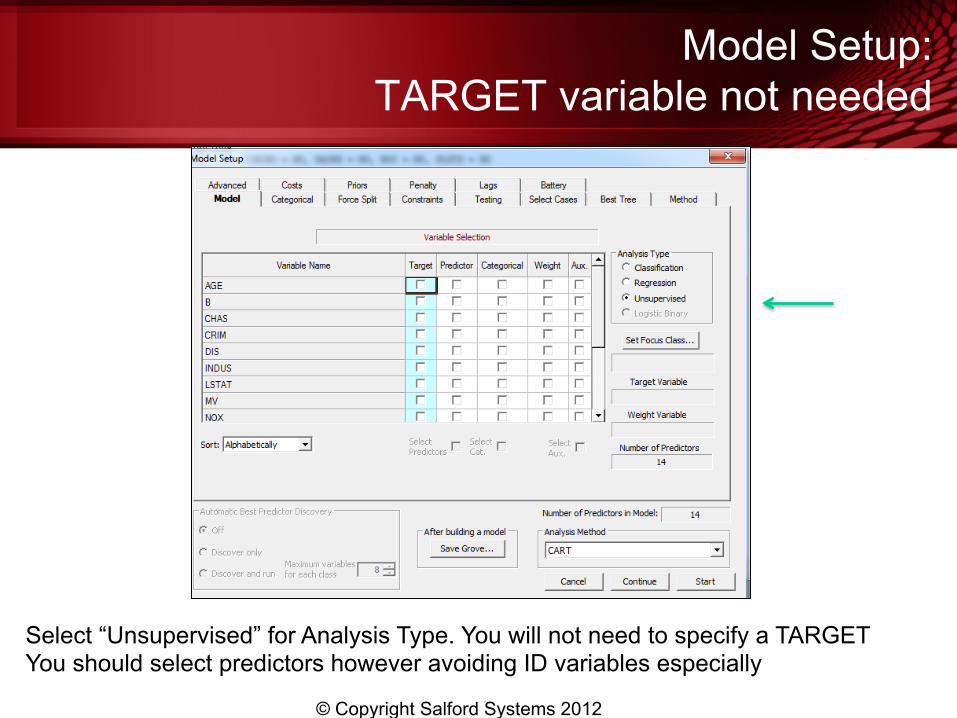
Model Setup: TARGET variable not needed


Select “Unsupervised” for Analysis Type. You will not need to specify a TARGET You should select predictors however avoiding ID variables especially

We elected to exclude the usual target


Note that MV is unchecked (and it is the only variable unchecked) It could have been included but we know MV will forcefully create clusters

Set minimum size limits on terminal nodes


Smallest terminal node allowed will be 10 records Smallest node allowed to be a parent (and thus split) will be 25 records

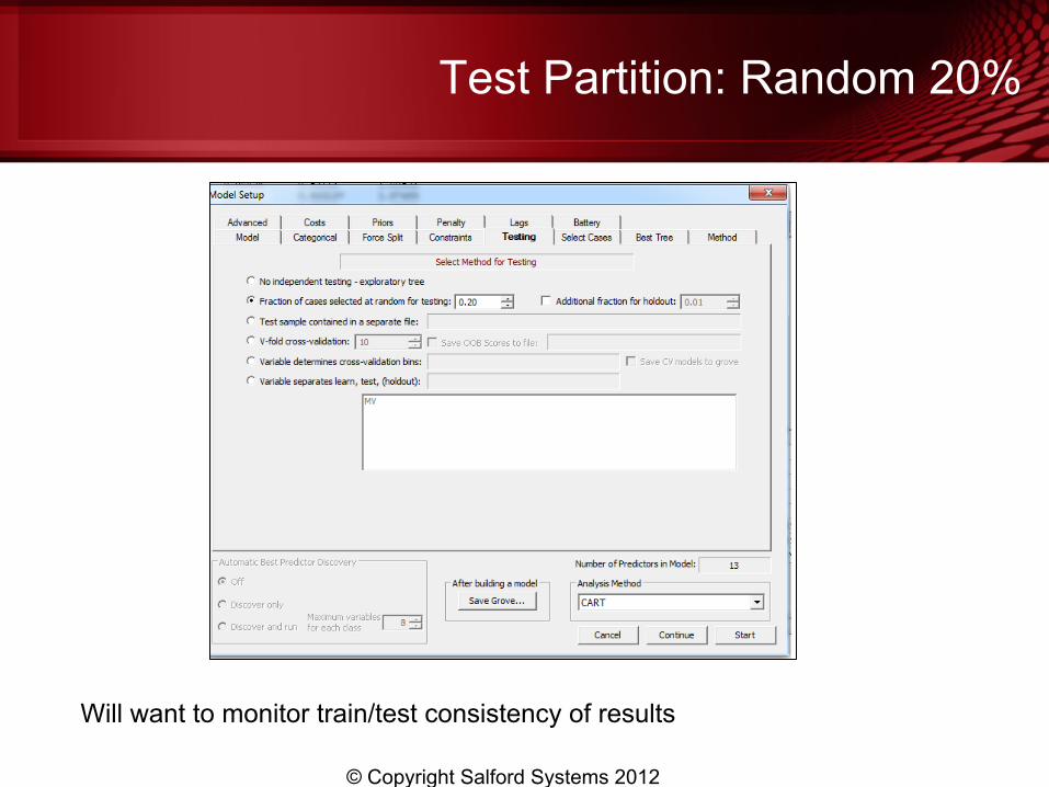
Test Partition: Random 20%


Will want to monitor train/test consistency of results

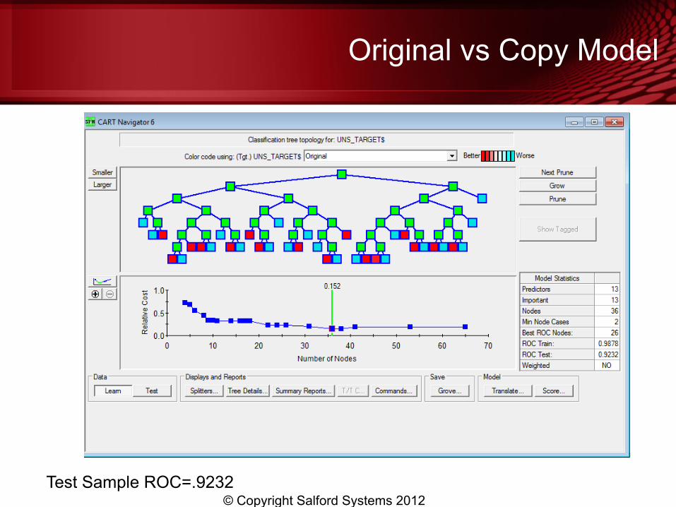
Original vs Copy Model

© Copyright Salford Systems 2012 Test Sample ROC=.9232

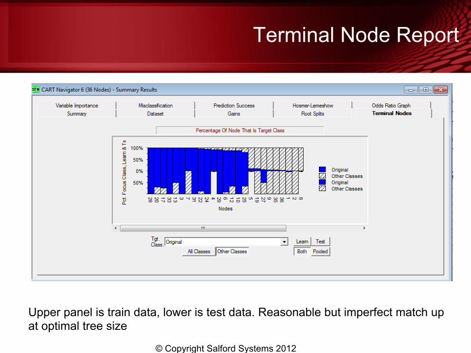
Terminal Node Report


Upper panel is train data, lower is test data. Reasonable but imperfect match up at optimal tree size

Better Matchup in 9-node tree


Terminal Node display is from Summary reports button on navigator

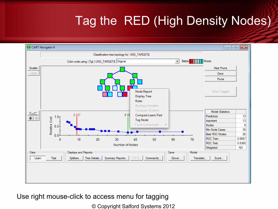
Tag the RED (High Density Nodes)


Use right mouse-click to access menu for tagging

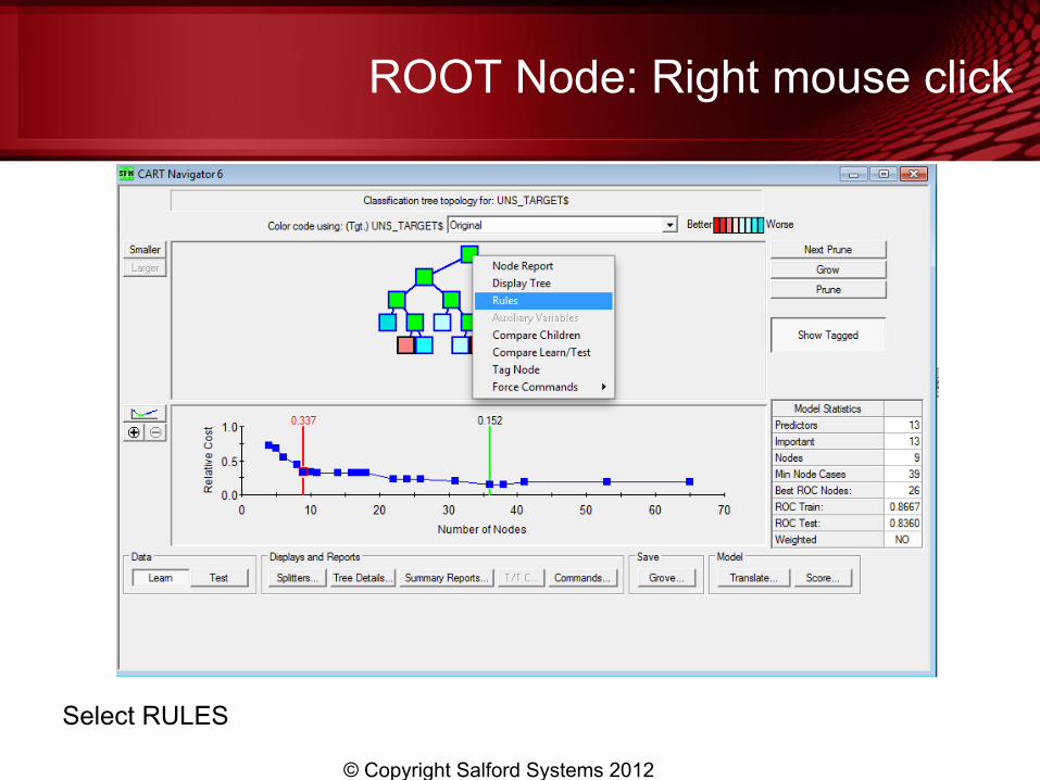
ROOT Node: Right mouse click


Select RULES

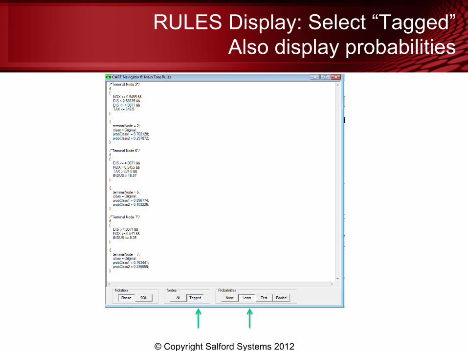
RULES Display: Select “Tagged” Also display probabilities


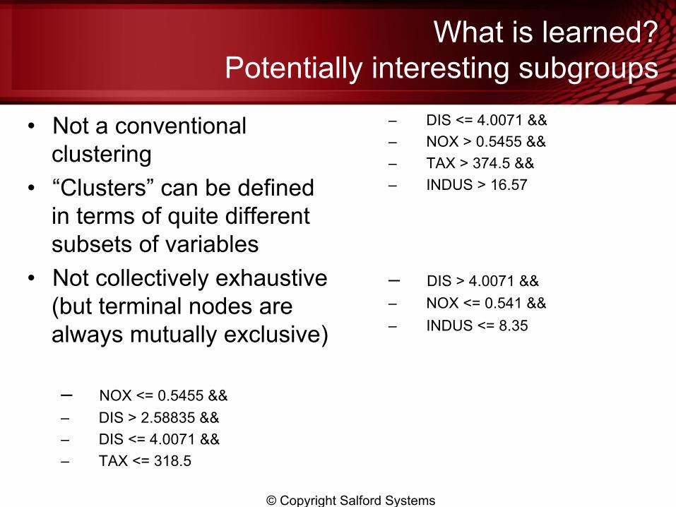
What is learned? Potentially interesting subgroups

•  Not a conventional clustering

•  “Clusters” can be defined in terms of quite different subsets of variables

•  Not collectively exhaustive (but terminal nodes are always mutually exclusive) –  NOX <= 0.5455 && –  DIS > 2.58835 && –  DIS <= 4.0071 && –  TAX <= 318.5

–  DIS <= 4.0071 && –  NOX > 0.5455 && –  TAX > 374.5 && –  INDUS > 16.57

–  DIS > 4.0071 && –  NOX <= 0.541 && –  INDUS <= 8.35


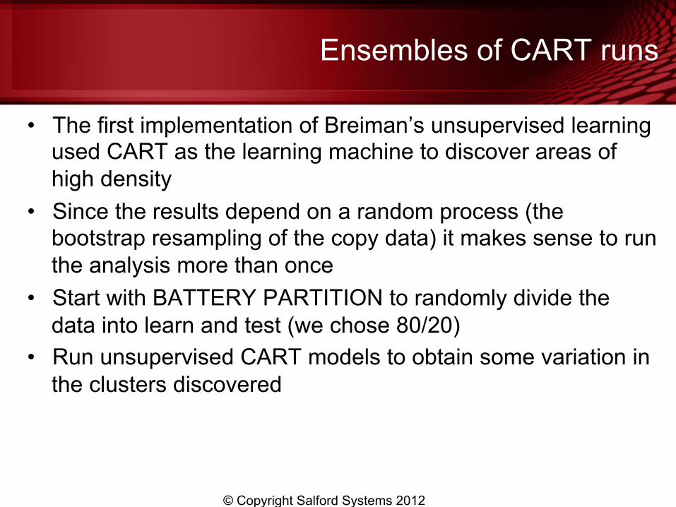
Ensembles of CART runs

•  The first implementation of Breiman’s unsupervised learning used CART as the learning machine to discover areas of high density

•  Since the results depend on a random process (the bootstrap resampling of the copy data) it makes sense to run the analysis more than once

•  Start with BATTERY PARTITION to randomly divide the data into learn and test (we chose 80/20)

•  Run unsupervised CART models to obtain some variation in the clusters discovered


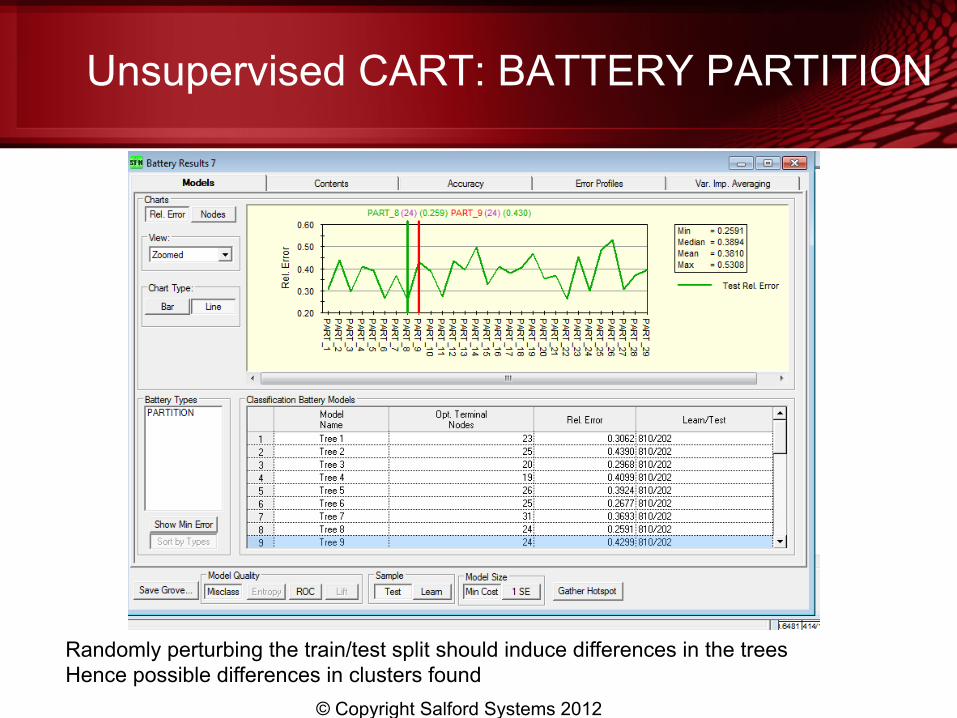
Unsupervised CART: BATTERY PARTITION


Randomly perturbing the train/test split should induce differences in the trees Hence possible differences in clusters found

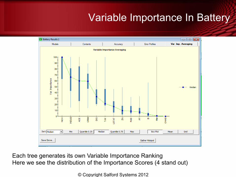
Variable Importance In Battery


Each tree generates its own Variable Importance Ranking Here we see the distribution of the Importance Scores (4 stand out)

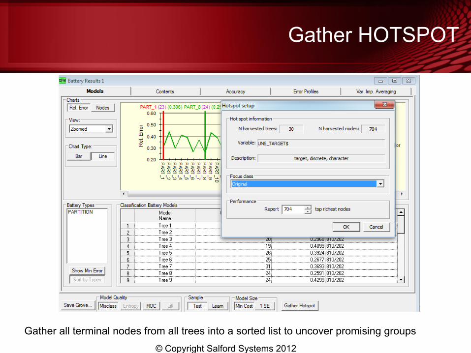
Gather HOTSPOT


Gather all terminal nodes from all trees into a sorted list to uncover promising groups

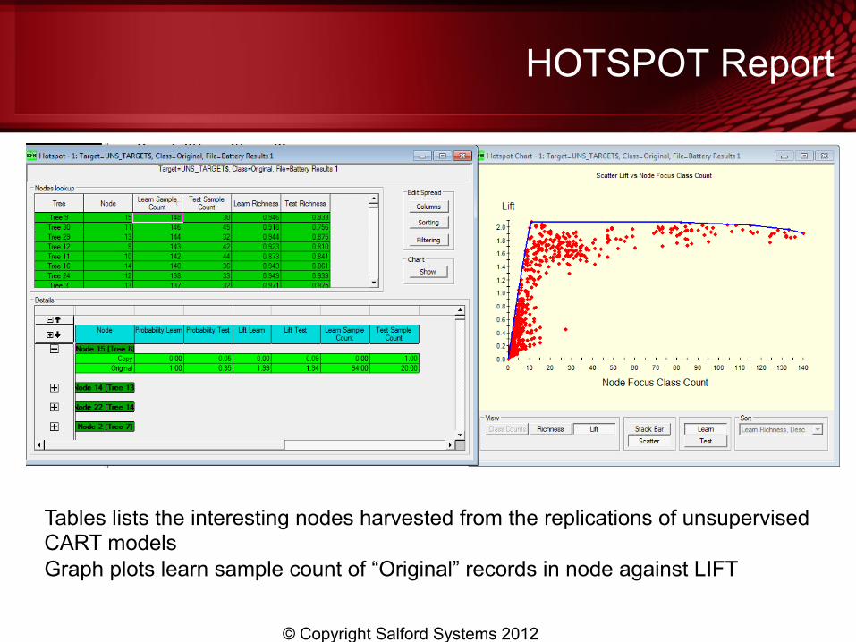
HOTSPOT Report


Tables lists the interesting nodes harvested from the replications of unsupervised CART models Graph plots learn sample count of “Original” records in node against LIFT

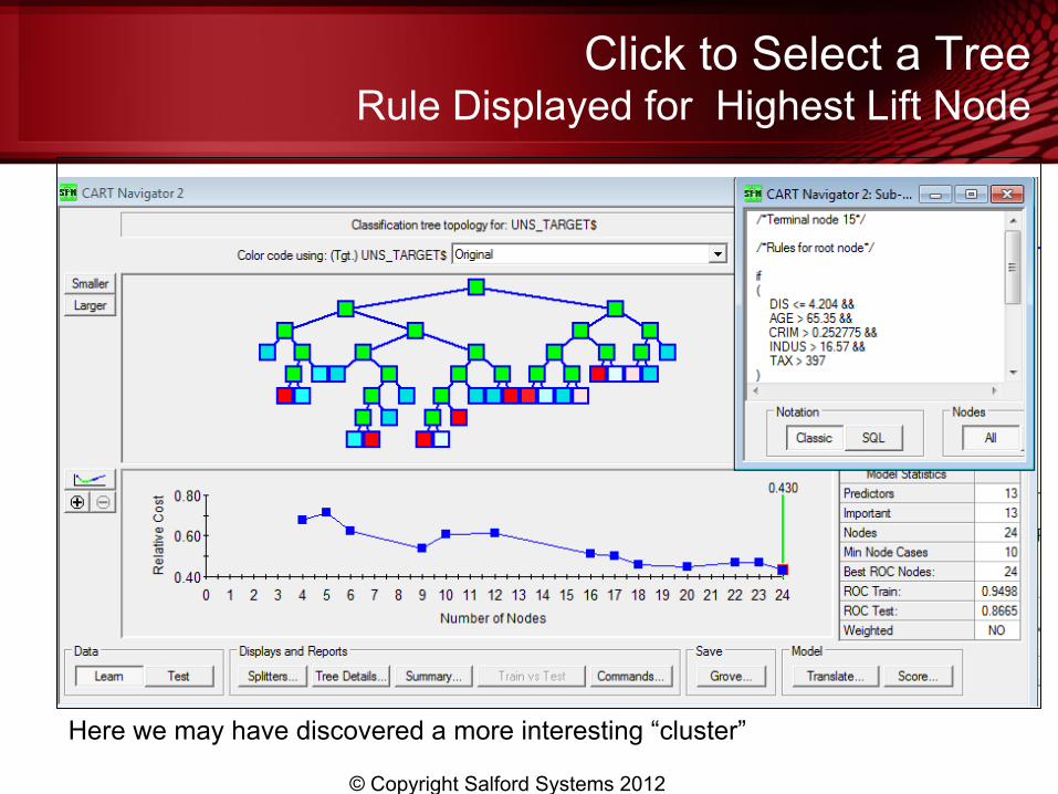
Click to Select a Tree Rule Displayed for Highest Lift Node


Here we may have discovered a more interesting “cluster”

Documents

Salford Systems Predictive Modeler Unsupervised Learning1.salford-systems.com/.../docs/unsupervised_learning_slides.pdf · Salford Systems Predictive Modeler Unsupervised Learning