Safety and Operational Characteristics of Lane Widths on Urban An

Clemson UniversityTigerPrints

All Theses Theses

1-1-2013

Safety and Operational Characteristics of LaneWidths on Urban and Rural Roadways A SimulatorStudyMeredith LaDueClemson University, [email protected]

Follow this and additional works at: http://tigerprints.clemson.edu/all_thesesPart of the Civil Engineering Commons

Please take our one minute survey!

This Thesis is brought to you for free and open access by the Theses at TigerPrints. It has been accepted for inclusion in All Theses by an authorizedadministrator of TigerPrints. For more information, please contact [email protected].

Recommended CitationLaDue, Meredith, "Safety and Operational Characteristics of Lane Widths on Urban and Rural Roadways A Simulator Study" (2013).All Theses. Paper 1828.

http://tigerprints.clemson.edu?utm_source=tigerprints.clemson.edu%2Fall_theses%2F1828&utm_medium=PDF&utm_campaign=PDFCoverPages

http://tigerprints.clemson.edu/all_theses?utm_source=tigerprints.clemson.edu%2Fall_theses%2F1828&utm_medium=PDF&utm_campaign=PDFCoverPages

http://tigerprints.clemson.edu/theses?utm_source=tigerprints.clemson.edu%2Fall_theses%2F1828&utm_medium=PDF&utm_campaign=PDFCoverPages

http://tigerprints.clemson.edu/all_theses?utm_source=tigerprints.clemson.edu%2Fall_theses%2F1828&utm_medium=PDF&utm_campaign=PDFCoverPages

http://network.bepress.com/hgg/discipline/252?utm_source=tigerprints.clemson.edu%2Fall_theses%2F1828&utm_medium=PDF&utm_campaign=PDFCoverPages

https://clemsonlibraries.qualtrics.com/SE/?SID=SV_6yTWgjf0SeA95Ln

http://tigerprints.clemson.edu/all_theses/1828?utm_source=tigerprints.clemson.edu%2Fall_theses%2F1828&utm_medium=PDF&utm_campaign=PDFCoverPages

mailto:[email protected]

SAFETY AND OPERATIONAL CHARACTERISTICS OF LANE WIDTHS ON

URBAN AND RURAL ROADWAYS

A DRIVING SIMULATOR STUDY

A Thesis

Presented to

the Graduate School of

Clemson University

In Partial Fulfillment

of the Requirements for the Degree

Master of Science

Civil Engineering

by

Meredith LaDue

December 2013

Accepted by:

Dr. Jennifer H. Ogle, Committee Chair

Dr. Wayne A. Sarasua

Dr. William J. Davis

ii

ABSTRACT

The primary goal for this study was to further evaluate and assess the effect of

lane width on the safety and operation of roadways in South Carolina. Due to various site

conditions that affect the safety and operations of roadways, highway design engineers

often face many challenges when developing appropriate road design standards. To

investigate specific site conditions for the South Carolina Department of Transportation

(SCDOT) a research study took place. In 2011, Part 1 of this research included field

studies conducted by Kevin Baumann and Trey Jordan. Due to the various limitations of

the field studies it was evident that additional research needed to take place.

This study (Part 2) uses a driving simulator study to examine three different lane

and shoulder width combinations on a rural curvy two-lane highway to determine the

effects on lateral position. These roadways were composed of various curves and straight

sections with a speed limit of 50 miles per hour. The study also examined how three

different two-way left turn lane (TWLTL) widths affected gap acceptance and

maneuverability within the lane for a three lane highway with a center lane (3T) and a

five lane highway with a center lane (5T). Below is a list of all the conditions that were

tested.

Combinations

12 ft. lane width, no paved shoulder

12 ft. lane width, 2 ft. paved shoulder

10 ft. lane width, 2 ft. paved shoulder

iii

TWLTL Widths

12 ft.

14 ft.

16 ft.

The simulated scenarios were designed to provide comparable data among the three

roadway combinations and comparisons between three TWLTL widths. Together the

results from this study and from Part 1 will coalesce to form design recommendations

regarding the selection of standard lane and shoulder widths for new projects in South

Carolina.

iv

ACKNOWLEDGEMENTS

First and foremost I want to thank my advisors Dr. Jennifer Ogle and Dr. Wayne

Sarasua for allowing me to be a part of the team for this project and giving me the

opportunity to complete my Masters. I am truly grateful for their support, hard work and

dedication that they have constantly provided for this project and throughout my stay at

Clemson University. Additionally, I would like to thank Dr. Jeff Davis for his support

and encouragement throughout the study.

I would also like to acknowledge my team of hard working students that helped

throughout the duration of this project. Completing this study would not have possible

without your hard work and diligence. Thank you Kweku Brown and Vijay Bendigeri for

all of your help and hard work spent designing the scenarios and testing the participants. I

also want to thank Brian Maleck for helping during the testing phase. Additional thanks

go out to Xi Zhao and Adika Mammadrahimli for their help with data analysis. Lastly, I

want to give thanks to Matt Chrisler for all his help and expertise during the design

process. Once again I want to thank you all for your dedication and hard work for this

project was truly a team effort.

v

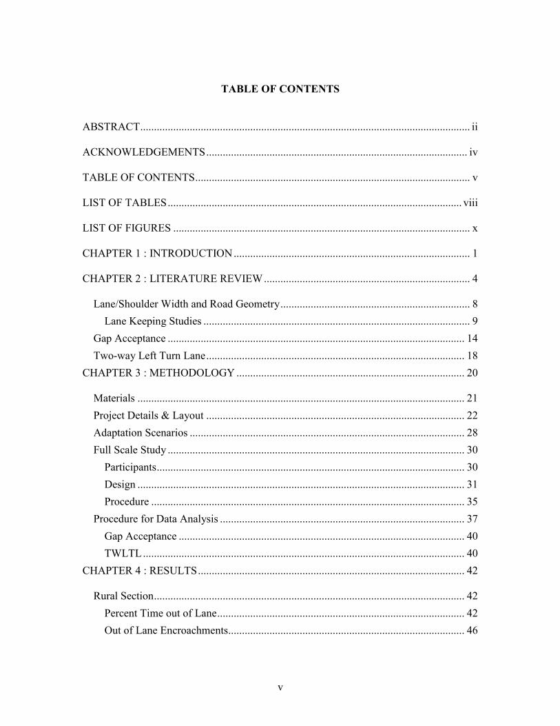
TABLE OF CONTENTS

ABSTRACT ........................................................................................................................ ii

ACKNOWLEDGEMENTS ............................................................................................... iv

TABLE OF CONTENTS .................................................................................................... v

LIST OF TABLES ........................................................................................................... viii

LIST OF FIGURES ............................................................................................................ x

CHAPTER 1 : INTRODUCTION ...................................................................................... 1

CHAPTER 2 : LITERATURE REVIEW ........................................................................... 4

Lane/Shoulder Width and Road Geometry ..................................................................... 8

Lane Keeping Studies ................................................................................................. 9

Gap Acceptance ............................................................................................................ 14

Two-way Left Turn Lane .............................................................................................. 18

CHAPTER 3 : METHODOLOGY ................................................................................... 20

Materials ....................................................................................................................... 21

Project Details & Layout .............................................................................................. 22

Adaptation Scenarios .................................................................................................... 28

Full Scale Study ............................................................................................................ 30

Participants ................................................................................................................ 30

Design ....................................................................................................................... 31

Procedure .................................................................................................................. 35

Procedure for Data Analysis ......................................................................................... 37

Gap Acceptance ........................................................................................................ 40

TWLTL ..................................................................................................................... 40

CHAPTER 4 : RESULTS ................................................................................................. 42

Rural Section ................................................................................................................. 42

Percent Time out of Lane .......................................................................................... 42

Out of Lane Encroachments...................................................................................... 46

vi

Gap Acceptance ............................................................................................................ 53

3T Sections................................................................................................................ 53

Delay ......................................................................................................................... 57

Scenario Order .......................................................................................................... 59

5T Sections................................................................................................................ 63

Effects of Age on Gap Acceptance ............................................................................... 67

Trajectories ................................................................................................................... 68

CHAPTER 5 : DISCUSSION ........................................................................................... 70

Rural Section ................................................................................................................. 70

Gap Acceptance ............................................................................................................ 71

Trajectories ................................................................................................................... 72

Age Comparison ........................................................................................................... 73

CHAPTER 6 : CONCLUSION ........................................................................................ 74

Recommendations ..................................................................................................... 74

APPENDIX A ................................................................................................................... 81

Traffic Intervals ............................................................................................................ 81

3T .............................................................................................................................. 81

5T .............................................................................................................................. 81

5T Effective Gaps ..................................................................................................... 81

APPENDIX B ................................................................................................................... 82

Curve Boundaries.......................................................................................................... 82

Scenario 1 and 2 ........................................................................................................ 82

Scenario 3.................................................................................................................. 83

APPENDIX C ................................................................................................................... 85

Script to Conduct Experiment ....................................................................................... 85

APPENDIX D ................................................................................................................... 93

Participant Data Sheets ................................................................................................. 93

APPENDIX E ................................................................................................................... 97

Participant Data ............................................................................................................. 97

vii

APPENDIX F.................................................................................................................. 100

Post Question Results on Driving Behavior ............................................................... 100

APPENDIX G ................................................................................................................. 101

Recommendations ....................................................................................................... 101

REFERENCES ............................................................................................................... 109

viii

LIST OF TABLES

Table 2.1: Driving simulation and on the road studies comparison (Hein, 2007) .............. 6

Table 3.1: Curve radii per scenario for rural section ........................................................ 24

Table 3.2: Participant data ................................................................................................ 30

Table 3.3: Rural undivided highway variables-Part 1(Baumann and Jordan, 2012) ........ 32

Table 4.1: 12 ft. lane no shoulder- Percent time out of lane data ..................................... 43

Table 4.2: 12 ft. lane 2 ft. shoulder- Percent time out of lane data ................................... 43

Table 4.3: 10 ft. lane 2ft. shoulder- Percent time out of lane data .................................... 44

Table 4.4: Total Percent Time out of lane for Curves by percentile ................................. 46

Table 4.5: Left and right encroachments for Scenario 1&2 ............................................. 47

Table 4.6: Curve details for Scenario 1&2 ....................................................................... 47

Table 4.7: Left and right encroachments for Scenario 3 ................................................... 48

Table 4.8: Curve details for Scenario 3 ............................................................................ 48

Table 4.9: Total number of encroachments ...................................................................... 49

Table 4.10: Lane position statistics ................................................................................... 51

Table 4.11: Ordered differences report ............................................................................. 51

Table 4.12: Analysis of Variance for second 3T turn ....................................................... 55

Table 4.13: Gap Data for All 3T turns .............................................................................. 56

Table 4.14: Gap Data for First 3T turn ............................................................................. 56

Table 4.15: Gap Data for Second 3T turn ......................................................................... 56

Table 4.16: Average Delay (s) .......................................................................................... 57

Table 4.17: Cumulative delay per traffic interval for 3T turns ......................................... 59

ix

Table 4.18: Gap Data for Scenario Order ......................................................................... 60

Table 4.19: Analysis of Variance for Scenario Order....................................................... 61

Table 4.20: Pairwise Comparisons for Scenario Order .................................................... 61

Table 4.21: Delay data based on scenario order ............................................................... 62

Table 4.22: Gap data for all 5T turns ................................................................................ 63

Table 4.23: Analysis of Variance for all 5T turns ............................................................ 64

Table 4.24: Delay data for all 5T turns ............................................................................. 65

Table 4.25: Cumulative delay per traffic interval for 5T turns ......................................... 66

Table 4.26: Gap data for young participants ..................................................................... 67

Table 4.27: Gap data for middle-old participants ............................................................. 67

Table 6.1: Magnitude of encroachments ........................................................................... 75

Table 6.2: Highway Safety Manual combination comparison.......................................... 76

Table 6.3: Part 1 recommendations .................................................................................. 78

x

LIST OF FIGURES

Figure 2.1: Effect of lane width on standard deviation of lane position ............................. 9

Figure 2.2: Mean lateral position of the vehicle in the lane (Dijksterhuis et al., 2010) .... 10

Figure 2.3: (Dijksterhuis et al., 2010) ............................................................................... 11

Figure 2.4: Lane position (Ben-Bassat and Shinar, 2011) ................................................ 12

Figure 2.5: Effect of shoulder width on mean lateral position

(Ben-Bassat and Shinar, 2011) ......................................................................................... 13

Figure 2.6: Effect of roadway geometry on lane position standard deviations (Ben-Bassat

and Shinar, 2011) .............................................................................................................. 13

Figure 2.7: Traffic scenario design for left-turn gap acceptance (Yan et al., 2007) ......... 15

Figure 2.8: Gap acceptance as a function of subject's gender and age (Moussa et al.,

2012) ................................................................................................................................. 17

Figure 2.9: Roadway configuration (Manual, 2004) ........................................................ 18

Figure 3.1: Drive Safety DS600 driving simulator ........................................................... 22

Figure 3.2: Rural two-lane undivided roadway ................................................................ 23

Figure 3.3: Rural roadway geometry ................................................................................ 24

Figure 3.4: 5T section in HyperDrive ............................................................................... 26

Figure 3.5: 3T section in HyperDrive ............................................................................... 26

Figure 3.6 : Complete scenario layout in HyperDrive ...................................................... 27

Figure 3.7: First adaptation scenario- lane keeping .......................................................... 29

Figure 3.8: Distribution of urban 3T TWLTL widths from Part 1 of study ..................... 33

Figure 3.9: Distribution of urban 5T TWLTL widths from Part 1 of the study ............... 33

xi

Figure 3.10: Yellow follow car in 5T section ................................................................... 35

Figure 3.11: Lane position orientation .............................................................................. 38

Figure 3.12: Out of lane encroachment............................................................................. 38

Figure 3.13: Curve and straight section boundaries .......................................................... 39

Figure 3.14: Vehicle trajectory for 3T section .................................................................. 41

Figure 4.1: Scenario 1- Percent time out of lane in curves ............................................... 45



Figure 4.4: Scenario 1 (12,0) total encroachments ........................................................... 50

Figure 4.5: Scenario 2 (12',2') total encroachments .......................................................... 50

Figure 4.6: Scenario 3 (10',2') total encroachments .......................................................... 50

Figure 4.7: Effects of roadway geometry on vehicle encroachments ............................... 52

Figure 4.8: All 3T turns .................................................................................................... 54

Figure 4.9: Analysis of Variance for all 3T turns ............................................................. 54

Figure 4.10: Second 3T turn ............................................................................................. 55

Figure 4.11: Gap interval frequency for All 3T turns ....................................................... 57

Figure 4.12: Gap interval frequency for First 3T turn ...................................................... 58

Figure 4.13:Gap interval frequency for second 3T turn ................................................... 58

Figure 4.14: Average Gap for Scenario Order .................................................................. 60

Figure 4.15: Gap interval frequency for scenario order .................................................... 62

Figure 4.16: Average gap for all 5T turns......................................................................... 64

Figure 4.17: Gap interval frequency for 5T turns ............................................................. 65

xii

Figure 4.18: Vehicle trajectories for second 3T turn ........................................................ 69

Figure 6.1: South Carolina fatalities comparisons ............................................................ 77

1

CHAPTER 1 : INTRODUCTION

The main goal of this study is to determine the influence that flexible lane width

standards have on the safety and operation of roadways in South Carolina. In 2011, Part 1

of this research was conducted in which field studies were performed. Due to various

limitations from the field studies it was apparent that to fully investigate the effects of

variable lane widths, Part 2, a driving simulator study needed to take place. Throughout

Part 1, several limitations were discovered as the project progressed. As an observational

study, data was limited based on the availability of site specific parameters and what

could be observed in the field. It is no surprise that the majority of sites fell within a

small range of allowable limits set forth in the Highway Design Manual. Thus, the study

of flexible lane widths was limited by the lack of variable lane width combinations found

in the field. Due to such limitations, it was difficult to obtain and analyze an adequate

sample of roadways regarding the desired lane and shoulder width attribute combinations.

By using a driving simulator controlled tests can be performed and designed for the lane

and shoulder width combinations that could not be analyzed in Part 1. The addition of

this study will help further identify how South Carolina will benefit from implementing

more flexible lane width standards.

Based on the following objectives, the aim of this study is to ultimately provide

and build upon the design recommendations made from Part 1 pertaining to the selection

of standard lane and shoulder widths for new projects. The objectives for this experiment

are provided below:

2

1.) Analyze the effect lane and shoulder width combinations have on driver

performance.

2.) Analyze the effect of curves on lane position for various lane and shoulder

width combinations.

3.) Analyze the operational performance (gap acceptance and maneuverability) of

TWLTLs for minimum and maximum widths.

To incorporate all of these objectives into one study, three scenarios were

designed. Three different lane and shoulder width combinations were tested on a rural

curvy two-lane undivided highway. These combinations included a 12 ft. roadway with

no paved shoulder, a 12ft. roadway with a 2 ft. paved shoulder and a 10 ft. roadway with

a 2 ft. paved shoulder. These combinations were implemented to test their effect on

lateral position. Analyses for the TWLTLs were conducted on both a 3T and 5T. The

TWLTL widths were 12, 14 and 16 ft. Participants were instructed to make left turns out

of a development/ driveway into the TWLTL. Analyses were conducted to determine if

the width had any effect upon gap acceptance. Operational analysis of the TWLTL was

also examined based on how participants maneuvered in the center lane as a function of

the lane width.

The remainder of this document is composed of numerous chapters that expand

upon the various aspects of this study. Chapter 2 consists of a comprehensive literature

review of previous driving simulator studies that evaluated the effect of lane width on

driving behavior. Following the literature review is Chapter 3 which provides a detailed

3

description of the methods used to perform the study. Results from the study are

presented in Chapter 4 followed by a discussion in Chapter 5. Both of these chapters

provide findings regarding the effects of lane and shoulder width combinations on lane

position and out of lane encroachments and the effects of the TWLTL width on gap

acceptance and maneuverability. Lastly, Chapter 5 consists of final conclusions regarding

the objectives that were tested and recommendations for the SCDOT. Appendices are

also attached to expand upon findings and processes that took during the study.

4

CHAPTER 2 : LITERATURE REVIEW

While field studies are critical in learning about various roadway treatments, the

diversity of environments and driver characteristics often cause difficulty in conducting

comparative research. To be specific, adverse weather and unaccounted traffic congestion

can easily interfere with a study. Due to the various conditions, driving simulators have

proven to be an influential tool providing additional avenues for research. The unique

ability to design specific scenarios has increased our ability to explore and learn more

about driving behavior, driver responses, user performances and training. Simulators

allow researchers to emulate real life roadway conditions in a safe and practical manner.

As stated by van der Horst et al. “ Systematic control over the experimental conditions

with respect to road design elements, traffic management, other traffic, and

environmental conditions makes human factors research in a driving simulator attractive,

efficient and effective.” After performing their driving simulator study Godley et al.,

(2001) also stated that simulators enable “Experimental control, efficiency, expense,

safety and ease of data collection.” Given the ability to manipulate various environmental

factors and test multiple treatments, driving simulators have become an effective tool for

comparative research.

Despite the beneficial use of reducing risk and increasing safety, simulators also

have drawbacks- including potential simulator sickness. This syndrome is commonly

perceived as motion sickness as both conditions express similar side effects such as

nausea, headaches, sweating, disorientation and vomiting (Brooks et al., 2010) .While

driving a simulator, it is common for the body’s vestibular senses to perceive the

5

discontinuity between the visual and physical effects, thus causing these symptoms to

occur (Brown, 2012). Simulator sickness can be detrimental to an experiment by

undermining the effectiveness of training and causing various participants to drop out of

the study (Brooks et al., 2010) (de Winter et al., ). Additional limitations and challenges

of driving simulators focus on fidelity and validity. The quality of simulator use is often

determined by these two aspects (Riener, 2011). Fidelity refers to the level of realism

expressed by the simulation, while validity is “the degree to which behavior in a

simulator corresponds to behavior in real-world environments under the same conditions

(Riener, 2011).” Studies by (Engström et al., 2005) expressed a relationship between

these two variables in which high fidelity simulators provide a more realistic

environment, thus producing results of higher validity in comparison to a low fidelity

simulator. Costs and benefits between the two types of simulators and field studies can

be seen in the table below. As shown, the high fidelity simulation exceeds on the road

studies in all categories except degree of realism. Low fidelity simulators also exceed on

the road studies in most of the categories excluding degree of realism and ability to study

range of traffic conditions.

6

Table 2.1: Driving simulation and on the road studies comparison (Hein, 2007)

Based on the parameters of the study, funds, and availability of resources the

desired fidelity may be hard to obtain. The second quality-defining parameter and

constant challenge of simulator use is validity. Validity is the premise in which findings

from the simulated environment can be applied to the real world. It can be broken down

into two categories, physical validity and behavioral validity. Physical validity is

represented as the degree in which the simulator’s visual components, dynamics and

7

layout replicate the real world hence, fidelity (Brown, 2012; Blaauw, 1982). Behavioral

validity measures the similarity between driving behavior in the simulator compared to

behavior in the real world. The validity of a study can further be defined as absolute or

relative. Research suggests that validation is best tested by comparing driving in the

simulator to a real car while performing tasks that are extremely similar for both

conditions (Blaauw, 1982). When comparing variables between the simulated and real

world environment it is possible to achieve absolute or relative validity. Absolute validity

is established if the numerical values between the two systems are the same. Relative

validity is expressed when “the differences found between experimental conditions are in

the same direction, and have a similar or identical magnitude on both systems (Godley et

al., 2002).” Results from driving simulators are considered useful if relative validity is

achieved (Törnros, 1998).

In 1998 Wade and Hammond conducted a study testing the relative validity of

lateral lane position measurements. In the study 26 participants drove on simulated and

real-world rural roadways. By using several vehicle performance measures, kinematic

variables and a questionnaire comparing the two environments the team was able to

conclude relative validity based on lateral position.

8

Lane/Shoulder Width and Road Geometry

One of the main objectives of this study is evaluating the effect lane width,

shoulder width and roadway geometry has on driver perception and behavior. While

roadway design is typically associated with accident rate, there are very few studies that

investigate the effect roadway design features have on driver behavior. A specific

attribute affected by the driver’s perception of the road’s safety is speed. Several studies

suggest that narrow roads and lanes will reduce driver speed and produce safer driving

behavior (Shinar, 2007). It is predicted that drivers assess narrower roads as being more

dangerous thus causing the driver to slow down to avoid accidents and risky situations.

De Waard also proposed that narrower roadways require more mental effort for the driver

to maintain lane position. Contrary to these findings, other studies indicate a negative

effect between narrow shoulders and safe driving behavior. A study by Dewar and Olson

found that narrow shoulders on two-lane roads caused drivers to steer closer to the center

of the road increasing the risk of a head-on collision.

Another characteristic that can affect driver behavior is the roadway

geometry. To be specific, it requires more effort from the driver to stay in the lane while

driving through curves. The limited visibility when encountering a curve limits the

driver’s ability to perceive the route ahead which increases uncertainty (Martens et al.,

1997). It is often difficult to evaluate the effects of roadway geometry alone due to the

extreme influence that lane and shoulder width play on the driver’s perception. To help

understand and distinguish such effects many researchers have started to perform driving

simulator studies.

9

Lane Keeping Studies

Green et al. (1994) used the UMTRI driving simulator to test the relationship

between roadway geometry and driver performance. In this study eight participants drove

a series of six winding road segments with varying sight distance and widths ranging 15

to 24 ft. Results from the study revealed significant effects on the standard deviation of

lane positioning due to road width. It was also evident that the standard deviation of

lateral position increased as the road became wider and decreased as the sight distance

increased.

Figure 2.1: Effect of lane width on standard deviation of lane position

(Green et al., 1994)

10

In 2011, Dijksterhuis et al., used a driving simulator to observe lane position

between four levels of lane width: 3.00, 2.75, 2.50, 2.25 m. Subjects were also exposed to

high and low densities of oncoming traffic while driving each lane width section within

the scenario. Each section was designed identically on rural roads that consisted of 85%

curves with 382 m radii. The remaining 15% of the roadway was composed of straight

sections and intermittent towns that separated the four sections of altering roadway

widths. Results showed no significance between the different levels of lane width and

oncoming traffic density. Marginal significance was found between the 3.00 m and the

2.50 m lane width conditions and the 2.75 m and 2.50 m conditions. Though, no

statistical evidence or trend was found for lane position of the vehicle due to lane width

variations, Figure 2.3 indicates that further studies on the matter are required. Graph B

within this figure shows that participants drove over the lines the most while driving in

the 2.25 m lane width. As the lane width increased participants’ lane keeping

performance increased.

Figure 2.2: Mean lateral position of the vehicle in the lane (Dijksterhuis et al., 2010)

11

Figure 2.3: (Dijksterhuis et al., 2010)

A study conducted by Ben-Basset (2011) evaluated lane wandering as a function

of shoulder width and presence of guardrail. The paved shoulder widths evaluated were

0.5, 1.2 and 3.0 m. The roadway geometry in each scenario included right and left sharp

and shallow curves. Curve radii were set at 80 m and 380 m respectively. Roads in the

scenario were two- lane divided highways with two 4.5 m lanes in each direction. Results

from the study found an extreme deviation in variance for all three shoulder widths when

driving sharp left turns. Analysis also revealed significant effects of shoulder width on

the average lane position. Values for lane position were determined as the distance of the

center jersey to the center of the vehicle. This is shown in Figure 2.4.

12

Figure 2.4: Lane position (Ben-Bassat and Shinar, 2011)

Subjects drove significantly closer to the left lane with a 0.5 m shoulder than the

1.2 and 3.0 m shoulders. Average lane position values for these widths were 6.9, 7.1 and

7.3 m respectively. From these results it is evident that as the road shoulder became

wider the participants gravitated more towards the middle and right edge of the lane. The

trend can be seen in Figure 2.5. Additional analysis compared the standard deviation of

lane position against road geometry. From Figure 2.6 it is evident that the roadway

geometry had a significant impact on the driver’s ability to keep in the center of the right

lane. The large standard deviation of lane position for the sharp left turn indicates that the

participants were wandering along the lane and may have veered off the road.

13

Figure 2.5: Effect of shoulder width on mean lateral position

(Ben-Bassat and Shinar, 2011)

Figure 2.6: Effect of roadway geometry on lane position standard deviations (Ben-

Bassat and Shinar, 2011)

14

Gap Acceptance

Other essential aspects of this paper focus on the operational performance of two-

way left turn lanes (TWLTL) and gap acceptance. Gap acceptance as defined by the

Highway Capacity Manual (HCM) 2010 is “The process by which a driver accepts an

available gap in traffic to perform a maneuver.” This behavior is often seen at a two-way

stop- controlled intersection (TWSC). A TWSC intersection is one of the most commonly

used unsignalized intersections in the United States (Kittelson and Vandehey, 1991).

They are composed of a “major” street that is uncontrolled and a “minor” street that is

controlled by stop signs (Nabaee, 2011), (HCM, 2010). In this setting, gap acceptance

behavior is expressed when a vehicle on the minor street needs to cross the major street

and when a vehicle must make a left turn that crosses the path of the opposing movement.

This concept is also seen on midblock arterials when a driver must make a left turn out of

a development into a two-way left turn lane. All of these cases test the driver’s ability to

perceive a stream of dynamic oncoming traffic and evaluate the availability and

usefulness of the gaps to safely maneuver across through travel lanes(Zohdy et al.,

2010),(Nabaee, 2011). Gap also referred to as headway is further defined by the HCM

(2010) as the elapsed time between two successive vehicles as they pass a specific point

on the roadway measured from the same feature of both vehicles. The minimum gap that

a driver will accept is commonly known as the critical gap. It is assumed that drivers

would accept gaps equal to or larger than the critical gap and reject gaps that are less than

the critical gap (HCM, 2010). This parameter is typically used to determine the safety and

operational performance of TWSC intersections (Nabaee, 2011).

15

While gap acceptance is a common behavior many factors affect the

drivers’ decision making process in deeming a gap acceptable. External factors include

time of day effects, type of intersection control, intersection geometry, driver’s sight

distance, and speed of opposing vehicles (Zohdy et al., 2010). Studies have also led to

results indicating that driver characteristics age and gender influence a driver’s gap

acceptance behavior (Moussa et al., 2012).

In 2007 a driving simulator study was conducted by Yan et al. to determine the

effects of age and gender on drivers’ left turn gap acceptance behavior at a two-way stop

controlled intersection. The equipment used throughout the experiment was a high

fidelity driving simulator composed of five channels providing 180 degree field of view,

a motion base and Saturn Sedan cab. The study tested a total of 63 participants with

defining age categories of young (20-30), middle (31-55) and old (56-83). Vehicle gaps

in the two scenarios were arranged in a uniformly ascending order from 1 to 16 seconds.

Figure 2.7: Traffic scenario design for left-turn gap acceptance (Yan et al., 2007)

16

Results indicated that older drivers accepted larger gaps than middle age and

young drivers. Average gap values were 7.94 s, 6.20 s, and 6.29 s respectively. No

significant difference between young and middle age drivers was found. Gender results

showed that male drivers accept smaller gaps at an average of 6.38 s than females with an

average gap of 6.93 s. Such findings lead Yan et al. to suggest that female drivers and

older drivers are more conservative.

Another study that evaluated left-turn maneuvers at a two-way stop controlled

intersection was conducted by Moussa et al. (2011). This study integrated simulation with

a field study through the use of an augmented reality vehicle system, “ARV.” The system

is a tool installed in a vehicle that allows the driver to see an augmented video where

virtual objects can be added to the real-world view in real time. A total of 44 participants

drove one scenario where they made a left-turn maneuver at a two-way stop controlled

intersection. Results revealed that all participants accepted gaps in a range of 4 to 9 s.

Older drivers in the study accepted larger gaps averaging 7.36 s compared to younger

drivers who averaged 6.20 s gaps. Agreeing with Yan, Moussa’s findings suggest that

older drivers are the most conservative (Yan et al., 2007). The results also found no

significance between gender and gap acceptance. The frequencies of gaps taken

throughout the study are expressed in Figure 2.8.

17

Figure 2.8: Gap acceptance as a function of subject's gender and age (Moussa et al.,

2012)

Due to various factors, the critical gap for a specific maneuver can vary greatly. It

has also been found that waiting time can affect a driver’s gap acceptance behavior. As

the waiting time increases the driver will become more inclined to take the risk of

accepting a smaller gap. Results from Xiaoming et al’s study found that after a long wait

time many drivers would accept shorter gaps that they had previously rejected.

18

Two-way Left Turn Lane

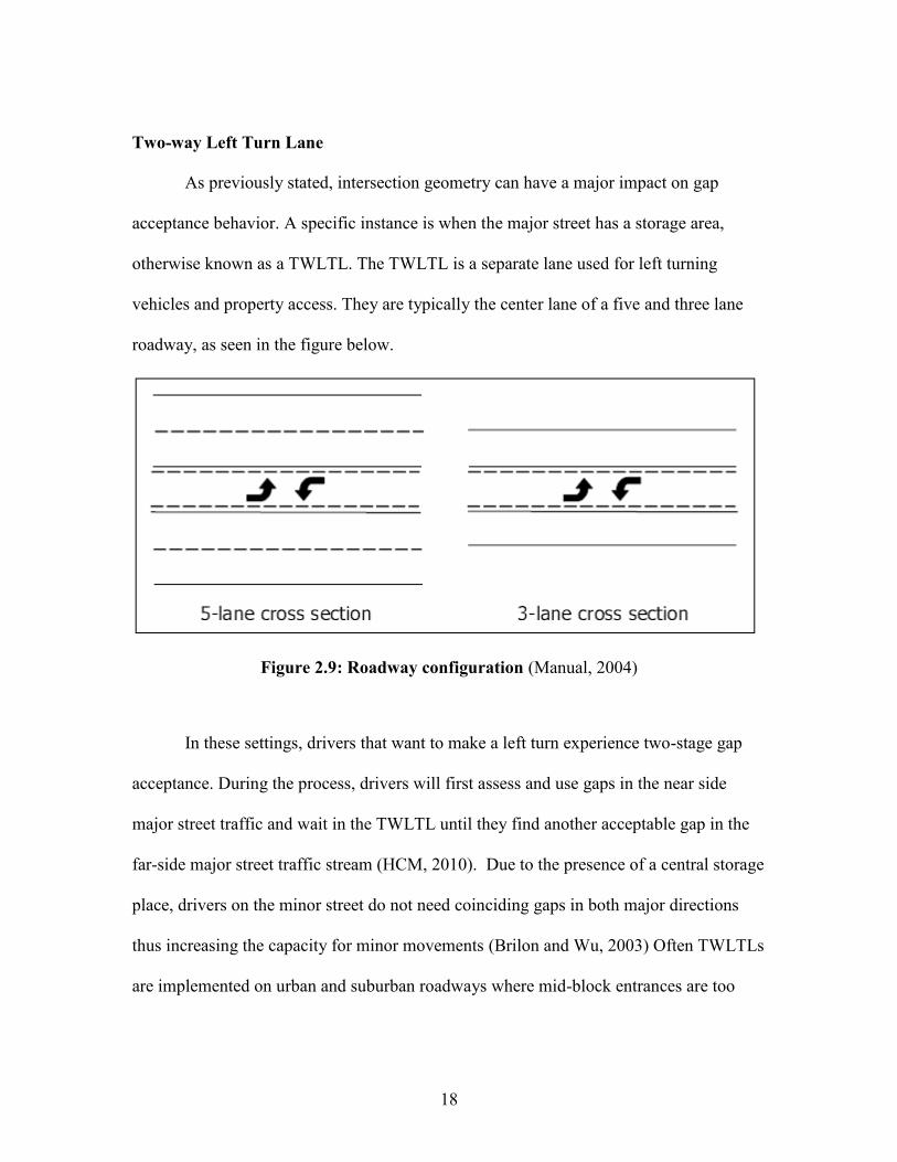
As previously stated, intersection geometry can have a major impact on gap

acceptance behavior. A specific instance is when the major street has a storage area,

otherwise known as a TWLTL. The TWLTL is a separate lane used for left turning

vehicles and property access. They are typically the center lane of a five and three lane

roadway, as seen in the figure below.

Figure 2.9: Roadway configuration (Manual, 2004)

In these settings, drivers that want to make a left turn experience two-stage gap

acceptance. During the process, drivers will first assess and use gaps in the near side

major street traffic and wait in the TWLTL until they find another acceptable gap in the

far-side major street traffic stream (HCM, 2010). Due to the presence of a central storage

place, drivers on the minor street do not need coinciding gaps in both major directions

thus increasing the capacity for minor movements (Brilon and Wu, 2003) Often TWLTLs

are implemented on urban and suburban roadways where mid-block entrances are too

19

close for turn lanes or when the percentage of turning volumes is high causing congestion

for through lanes. Studies suggest that adding a TWLTL on roadways under these

conditions with can result in improved safety and capacity (Manual, 2004). A study

conducted in Minnesota between 1991 and 1993 revealed that three lane roadways with a

TWLTL are about 27% safer than a four lane undivided roadway and a five lane roadway

with a TWLTL is approximately 41% safer than a four lane undivided roadway(Manual,

2004). Lane width guidelines for these facilities typically vary by state. Ranges depicted

by A policy of Geometric Design of Highways and Streets, “AASHTO Greenbook,”

include 10 to 12 ft. for urban/suburban arterials and 10 to 16 ft. for urban/suburban

collectors. While there are many studies that evaluate the change in the operational

performance of the roadway through the addition of a TWLTL very few have focused on

the effects produced by the TWLTL width. The lack of research in this area further

encourages the necessity for further studies. To gain more knowledge the simulator study

performed in this paper analyzed the effect varying TWLTL widths had on driver

maneuverability and gap acceptance.

20

CHAPTER 3 : METHODOLOGY

The purpose of this study was to evaluate three main objectives:

1. Test and analyze the effect lane and shoulder width combinations have on driver

performance

2. Test the effect of curves on lane position for various lane/shoulder width

combinations

3. Test operational performance of TWLTL for minimum and maximum widths

This study evaluated how various roadway design elements affect driver behavior.

Treatment effects were compared through the use of a driving simulator. The study was

conducted through a series of five different phases: 1.) Determine study procedures and

obtain IRB approval 2.) Scenario Development 3.) Scenario Review 4.) Full study 5.)

Data Analysis. The first step of the study included outlining the experimental procedure

for testing subjects. Prior to using the simulator it was imperative to ensure that all

requirements for the experiment were met and to gain approval from Clemson’s

Institutional Review Board for the testing of human subjects. The second phase consisted

of scenario development. In this part of the study, all experimental parameters were

implemented into the design of three scenarios. These encompassed three lane width and

shoulder width combinations and six two-way –left turn lane (TWLTL) treatments. Once

all of the scenarios were designed, sample tests were conducted to test the various

capabilities and limitations of the simulator and examine the measured variables of lane

position, speed, gap acceptance and vehicle heading. For these sample experiments

21

various South Carolina Department of Transportation Officials and graduate students

were tested and produced feedback on the scenario layout. After making several

alterations to improve the experiment, the full scale study took place. In this phase,

subjects drove five adaptation scenarios to acclimate them to the simulator followed by

the three treatment scenarios. During the full scale study, data was collected for all

participants, thus leading to the final phase of data analysis.

The next four sections will provide extensive detail on the materials used, project

details, the scenario layout, participants and data analysis procedure.

Materials

This experiment was conducted through the use of Clemson University’s driving

simulator located in Brackett Hall. The simulator is a high performance and high fidelity

product produced by Drive Safety. It has five projection screens and three configurable

rear view mirrors. The simulator has a partial Ford Focus cab with standard driver

controls and a full width front interior. The car functions with an automatic transmission

and has a 3-D audio system to incorporate the sounds of the engine and traffic noise to

the driving experience. The simulator also sits on a platform enabling longitudinal

movement.

The software for the simulator is composed of three different components:

Vection, Dashboard and HyperDrive Authoring Suite. Vection is the component that runs

the simulation. The HyperDrive Authoring Suite is a windows-based software package

that enables the ability to design scenario layouts and manipulate various variables

relating to traffic, road side entities, and community types amongst others. The software

22

can also collect data on 25 user defined variables pertaining to lane position, acceleration,

deceleration, heading and more. Lastly, Dashboard is the interface that bridges the design

aspect of HyperDrive to a virtual reality. It transfers the newly developed scenarios in

HyperDrive to the driving simulator, thus allowing one to drive their design.

Figure 3.1: Drive Safety DS600 driving simulator

Project Details & Layout

The main objectives for this study were to test and analyze the effect lane and

shoulder width combinations have on driver performance, to test the effect of curves on

lane position for various lane/shoulder width combinations and to test the operational

performance of TWLTLs for minimum and maximum widths. The first two objectives

were accounted for in the beginning of the three scenarios. Each scenario started with a

23

1.5 mile rural curvy two lane highway. The roadway consisted of numerous curves and

straight sections. Specific curve radii and roadway layout for the scenarios can be seen in

Figure 3.3 and Table 3.1. Along this section, each scenario had different lane/shoulder

width combinations. These combinations included 12 ft. lanes and no shoulder for

Scenario 1, 12 ft. lanes and a 2 ft. paved shoulder for Scenario 2 and 10 ft. lanes with a 2

ft. paved shoulder for Scenario 3. The speed limit for each roadway was set at 50 miles

per hour. Lane position and speed data was collected for this section to analyze the

number of right and left edge touches and percent time out of lane per curve. To reduce

the effect of speed on the measured variables a 10 miles per hour threshold was allowed.

An audio recording was set to say “Increase your speed” if the driver drove below 45

miles per hour and “Slow Down” if the driver exceeded 55 miles per hour.

Figure 3.2: Rural two-lane undivided roadway

24

Table 3.1: Curve radii per scenario for rural section

Scenario 1 and 2

Scenario 3

Curve Radius (m) Radius (ft)

Curve Radius (m) Radius (ft)

1 418.0 1371.4

8 1665.0 5462.6

2 378.0 1240.2

9 451.6 1481.6

3 416.8 1367.5

10 344.0 1128.6

4 352.7 1157.2

11 296.0 971.1

5 375.9 1233.3

12 370.0 1213.9

6 604.3 1982.6

13 654.0 2145.7

7 362.3 1188.6

Figure 3.3: Rural roadway geometry

25

Following the curvy section was a continuous town segment where subjects made

a total of four left turns into two-way-left turn lanes. Gap acceptance and vehicle position

were measured on both a three lane roadway with a center two-way left turn lane (3T)

and a five lane roadway with a center two-way left turn lane (5T). Two of the left turns

were made on a 3T roadway, and the remaining two were made on a 5T roadway.

Images of these roadways are expressed in Figure 3.4 and 3.5. Both roadway geometries

were tested with TWLTL widths of 12, 14 and 16 ft., creating a total of six combinations.

Scenario 1 tested TWLTL widths of 12 ft. for the 3T turns and 16 ft. for the 5T turns.

Scenario 2 tested 16 ft. for the 3T turns and 14 ft. for the 5Ts while Scenario 3 tested 14

ft. for the 3Ts and 12 ft. for the 5Ts. Overall, each scenario had the same layout

containing a rural curvy section, two 3T and two 5T sections. A comprehensive summary

and scenario layout image can be seen below.

26

Figure 3.4: 5T section in HyperDrive

Figure 3.5: 3T section in HyperDrive

27

Figure 3.6 : Complete scenario layout in HyperDrive

28

Scenario Summary

Scenario 1

Rural 3 mile section (12’ lane, no shoulder)

3T Section (12’ lanes, 12’ TWLTL)


Scenario 2

Rural 3 mile section (12’ lane, 2’ shoulder)



Scenario 3

Rural 3 mile section (10’ lane 2’ shoulder)



Adaptation Scenarios

To familiarize the participants with the driving simulator’s handling, five

adaptation scenarios were conducted. The first scenario taught the driver the basics of

lane position in the simulator. For this session, the driver drove on a straight road with a

speed limit of 45 miles per hour. In the middle of the front screen there were five dots

that would light up indicating the vehicle’s lane position: far left, left, center, right, and

far right. Participants were given the opportunity to drive this scenario twice for thirty

seconds to test and understand the different lane boundaries within the simulator. An

image of this can be seen in Figure 3.7.

29

Figure 3.7: First adaptation scenario- lane keeping

The second adaptation scenario practiced lane keeping on a curvy road with a

speed limit of 45 miles per hour. For this session, the driver did not have the aid of the

five dots on the screen indicating their lane position. The participants drove this scenario

for a full sixty seconds, and the number of right and left edge touches during this time

period were recorded. The third scenario practiced stopping. Throughout this session, the

drivers had to make a series of five stops. Data for this scenario showed how close the car

was to the stop bar. A participant performed well if an average of plus or minus two feet

was maintained. In the fourth adaptation scenario, the driver had to complete six left

turns. The purpose of this scenario was to familiarize the participants with the speed and

maneuverability required to perform a left turn. The fifth and final adaptation scenario led

30

the driver to make four right turns. Not only were these scenarios essential in

familiarizing participants with the driving simulator, they also helped identify subjects

prone to simulator sickness.

Full Scale Study

Participants

The full scale study was conducted for a total of 60 participants. From this total,

two age groups were identified. The first age group consisted of 40 young drivers

between the ages of 18 to 34. The second group consisted of 20 participants within the

age range of 35+ years. All participants were compensated fifteen dollars per hour for the

time they spent on the study. The max amount one participant could earn was thirty

dollars. Participants were recruited by advertising flyers and word of mouth. The table

below is a summary of all the participants that were tested, including those who were

unable to complete the study due to simulator sickness.

Table 3.2: Participant data

Female Male Total

Young 20 20 40

Middle 6 14 20

Dropout- Simulator Sickness 6 6 12

Total # of Participants - - 72

# Participants Data used - - 60

31

Design

To design the three experimental scenarios various steps were taken. One of the

first steps included determining the different lane and shoulder width combinations and

TWLTL widths to be tested. To do this, it was important to become familiar with the

driving simulator’s program, HyperDrive Authoring Suite where the scenarios were

created. This involved learning the functions of the program and identifying useable tiles

in its library. The tiles were small roadway segments that would be placed together to

form any desired scenario.

It was decided that the first part of each scenario would be the rural curvy two-

lane highway section in which the various lane and shoulder width combinations would

be tested. Based on the current SCDOT Highway Design Manual guidelines and the

availability of lane width tiles within the simulator’s library, 12 and 10 ft. lanes were

used in this section. The shoulder widths chosen for these lane widths were either a 2 ft.

paved shoulder or no shoulder. These values were determined based on the abundance of

roadway segments that had either no paved shoulder or a 2 ft. paved shoulder from Part 1

of this study.

32

Table 3.3: Rural undivided highway variables-Part 1(Baumann and Jordan, 2012)

This produced the roadway combinations of 12ft lanes and no paved shoulder for

Scenario 1, 12 ft. lanes with a 2 ft. paved shoulder for Scenario 2 and 10 ft. lanes with a

2 ft. paved shoulder for Scenario 3. To perfect this section of the scenarios a great deal of

work was done. One curvy rural tile had 6 ft. shoulders on either side of the roadway. To

create no shoulder for Scenario 1 and a 2 ft. shoulder for Scenario 2 various small grass

tiles had to be overlapped over the existing large shoulder. Since there was no 10 ft. rural

curvy tile, this tile had to be custom made by the designer of Drive Safety. The next step

taken to further evaluate this portion of the scenario was to determine the speed of the

roadway. It was assumed that the rural tile in each scenario had a superelevation value

of 6%. Based on the minimum radius, a design speed of 50 mph was determined from the

Policy of Geometric Design of Highways and Streets.

The next part of each scenario was the development of the town segments where

participants drove a series of four left turns into TWLTLs. For this step it was important

Independent

VariableCoefficient

Number of

Segments

c 10 53

c 11 161

c 12 109

d 0 222

d 2 101

e 35- 11

e 40-45 86

e 50-55 226

f Low 281

f Med 42

Moderate Grade g 68

Lane Width (ft)

Shoulder Width (ft)

Speed Limit (mph)

Driveway Density

(Driveways/Mile)

33

to choose TWLTL widths that would provide acceptable comparative data. Based on the

available tiles in the HyperDrive library and the distribution of TWLTL widths that were

measured in the field during Part 1 of this study, widths of 12, 14 and 16 ft. were used.

The distributions of TWLTL widths for 3T and 5T roadways from Part 1 of the study can

be seen in Figure 3.8 and 3.9. Several of these tiles had to be custom designed from

DriveSafety.

Figure 3.8: Distribution of urban 3T TWLTL widths from Part 1 of study

Figure 3.9: Distribution of urban 5T TWLTL widths from Part 1 of the study

33%

36%

16%

15%

URBAN 3T

10ft-11ft

12ft-13ft

14ft-15ft

16ft +

6%

22%

58%

14%

URBAN 5T

10ft-11ft

12ft-13ft

14ft-15ft

16ft +

34

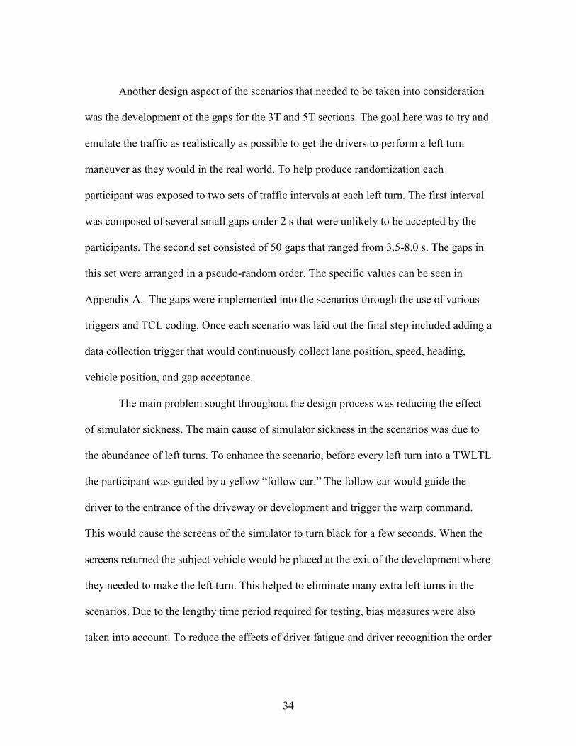
Another design aspect of the scenarios that needed to be taken into consideration

was the development of the gaps for the 3T and 5T sections. The goal here was to try and

emulate the traffic as realistically as possible to get the drivers to perform a left turn

maneuver as they would in the real world. To help produce randomization each

participant was exposed to two sets of traffic intervals at each left turn. The first interval

was composed of several small gaps under 2 s that were unlikely to be accepted by the

participants. The second set consisted of 50 gaps that ranged from 3.5-8.0 s. The gaps in

this set were arranged in a pseudo-random order. The specific values can be seen in

Appendix A. The gaps were implemented into the scenarios through the use of various

triggers and TCL coding. Once each scenario was laid out the final step included adding a

data collection trigger that would continuously collect lane position, speed, heading,

vehicle position, and gap acceptance.

The main problem sought throughout the design process was reducing the effect

of simulator sickness. The main cause of simulator sickness in the scenarios was due to

the abundance of left turns. To enhance the scenario, before every left turn into a TWLTL

the participant was guided by a yellow “follow car.” The follow car would guide the

driver to the entrance of the driveway or development and trigger the warp command.

This would cause the screens of the simulator to turn black for a few seconds. When the

screens returned the subject vehicle would be placed at the exit of the development where

they needed to make the left turn. This helped to eliminate many extra left turns in the

scenarios. Due to the lengthy time period required for testing, bias measures were also

taken into account. To reduce the effects of driver fatigue and driver recognition the order

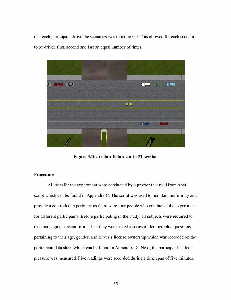
35

that each participant drove the scenarios was randomized. This allowed for each scenario

to be driven first, second and last an equal number of times.

Figure 3.10: Yellow follow car in 5T section

Procedure

All tests for the experiment were conducted by a proctor that read from a set

script which can be found in Appendix C. The script was used to maintain uniformity and

provide a controlled experiment as there were four people who conducted the experiment

for different participants. Before participating in the study, all subjects were required to

read and sign a consent form. Then they were asked a series of demographic questions

pertaining to their age, gender, and driver’s license ownership which was recorded on the

participant data sheet which can be found in Appendix D. Next, the participant’s blood

pressure was measured. Five readings were recorded during a time span of five minutes.

36

Afterwards, the participants were asked to sit in the car as they were taught about

the various operations of the vehicle. Before driving the three test scenarios each

participant drove a series of five adaptation scenarios to familiarize them with the driving

simulator and test if they get motion sickness. A detailed explanation of the adaptation

scenarios can be found in the previous section under Project Details and Layout.

Throughout the adaptation scenarios participants were given breaks if they seemed

necessary. At the end of each driving session, adaptation and experimental, participants

were asked a series of motion sickness questions that were rated from 0-10, with 10 being

severe. Examples of these questions include, dizzy, light headed, nauseous, and sweaty.

The remaining questions can be found in the data sheet in Appendix D.

After the training sessions participants were instructed to drive as he/she would in

their own vehicles as they drove the test scenarios. These consisted of three scenarios that

lasted approximately 15 minutes each to complete. All three scenarios tested lane

position, gap acceptance and maneuverability into TWLTLs. Scenario differences lied in

the roadway geometry. To be specific, Scenario 1 tested lane position on 12 ft. lanes and

no paved shoulder for the rural section and gap acceptance and maneuverability on a 12

ft. TWLTL width for the two 3T turns and a 16 ft. TWLTL width for the two 5T turns.

Scenario 2 had a 12 ft. lane and 2 ft. paved shoulder for the rural section, 16 ft. TWLTL

width for the 3Ts and a 14 ft. TWLTL lane for the 5Ts. Lastly, Scenario 3 had 10 ft. lanes

with a 2 ft. shoulder for the rural section and 16 ft. TWLTL width for the 3Ts and 12 ft.

TWLTL width for the 5Ts. In between each of the test scenarios, the participants took a

break and were asked to complete a safety survey. The survey had various images of

37

different roadways where the participant was asked to rate the scenario in each picture

based on their perceived safety. At the very end of the testing session five readings of the

participant’s blood pressure were taken for a span of five minutes. The blood pressure

measurements and safety survey helped to distract participants from the actual variables

that were tested in the study.

Procedure for Data Analysis

Rural Section

Continuous data collected from the authoring computer included speed, lane

position, vehicle heading, and vehicle position among others. For the rural section the

primary variable was the vehicle lane position. Based on the vehicle lane position each

participant’s percent time out of lane per curve and total number of left or right edge

touches was calculated. Lane position values were defined by the driving simulator as the

distance between the center of the car to the center of the traveling lane. The value was

negative if the center of the car moved to the left of the lane and positive if the car moved

to the right. Given continuous lane position data for this roadway segment percent time

out of lane and the number of out of lane encroachments were calculated for each

participant. The vehicle was considered to be out of lane if any portion of the vehicle

touched or crossed the white line on the right side of the lane or the double yellow line to

the left of the lane. An example of this can be seen in Figure 3.12.

38

Figure 3.11: Lane position orientation

Figure 3.12: Out of lane encroachment

Since the vehicle was a 5.11 ft. wide Ford Focus and the lane was 12 ft. for

Scenario 1 and 2, participants had to have lane position values that exceeded 1.0488 or

below -1.0488 to be considered out of the lane. Since Scenario 3 had a 10 ft. lane

participants were considered out of the lane if the lane position values were greater than

.744 or less than -.744. Then each curve and straight section was designated by their

39

starting and ending X, Y coordinates. The specific coordinates chosen for each segment

can be found in Appendix B. Based on these boundaries the number of right and left edge

touches and percent time out of lane was calculated for each section.

Figure 3.13: Curve and straight section boundaries

40

Gap Acceptance

Gap data from the study was analyzed descriptively and statistically. For each

scenario the mean and standard deviation was computed separately for 3T and 5T turns.

To see if there was any statistical significance between the average gaps per scenario for

the 3T turns a randomized block design was implemented. In this design, the different

lane widths in each scenario were the treatment and the block factor was the participant.

Since many participants waited the longest at their first 3T in their first scenario, another

evaluation was done after removing the first turn for each participant. The first turn for

every participant in each scenario had to be removed to reduce repeated measures so that

each participant contributed an equal amount of data points per scenario. A randomized

block design was also used for the 5T gap data to see if lane width had an effect on gap

acceptance.

TWLTL

Another method used to analyze how the width of the TWLTL affects its

operational performance was by creating vehicle trajectories. From these trajectories

relationships between the TWLTL width and the participants’ maneuverability became

more apparent. For this study, trajectories for the second 3T for 30 participants were

drawn by applying the vehicle’s X and Y coordinates into AutoCAD. Two different

layers of a line and car were used to draw the trajectories as seen in image B and C of

Figure 3.14. For the scope of this study the number of encroachments for the 30

participants in each scenario was analyzed. Additional analysis in a following paper will

be based off of the proportion of time the vehicle was out of the TWLTL for a designated

41

distance. This was calculated by first offsetting the vehicle’s path by one foot increments

which can be seen in Figure 3.14. Then all of the one foot lines within the boxed area

were evaluated. The subject was considered out of the lane if the line crossed the black

boundary that is drawn in image A of Figure 3.14.

A B C

Figure 3.14: Vehicle trajectory for 3T section

42

CHAPTER 4 : RESULTS

The data is expressed as three separate sections. First, descriptive data

representing the percent time out of lane and number of out of lane encroachments per

scenario for the rural section is presented. In the second section, comparisons between the

six TWLTL widths were statistically examined to determine if there was a significant

effect upon gap acceptance. Descriptive statistics were also performed to determine a

relationship between age and gender on gap acceptance. Lastly, several 3T trajectories

were examined to examine the effect different TWLTL widths have upon diver

maneuverability.

All inferential tests were completed as a completely random block design with an

alpha of .05. To reduce the variability of repeated measures the participant was the block

and the scenarios were the treatment. Based on the design multiple comparison ANOVAs

were produced. Additional simple effect tests were used if significant interactions were

found.

Rural Section

Percent Time out of Lane

The first step taken to analyze the curvy rural section for each scenario involved

calculating the percent out of lane for each participant in each scenario. For Scenario 1, a

total of 5 participants went out of lane on the 12 ft. roadway with no paved shoulder.

Scenario 2 had a 12 ft. roadway and a 2 ft. shoulder and had a total of 7 participants drive

out of the lane. Lastly, Scenario 3 had a 10 ft. roadway and a 2 ft. shoulder and had a high

43

of 14 participants drive out of the lane. Specific percent time out of lane values for each

scenario can be seen in the following tables. From the tables a pattern shows that many of

the participants that went out of the lane in Scenario 1 also proceeded to go out of the

lane in the following scenarios. After looking at age, gender and post test questions

regarding crashes and speeding tickets, no correlation between the participants was

found. Results from the analysis show very little difference between Scenario 1 and 2.

The reduced lane width in Scenario 3 proved to be more challenging as more participants

failed to stay within the lane boundaries.

Table 4.1: 12 ft. lane no shoulder- Percent time out of lane data

Table 4.2: 12 ft. lane 2 ft. shoulder- Percent time out of lane data

418 378 416.8 352.7 375.9 604.3 362.3

1371.4 1240.2 1367.5 1157.2 1233.3 1982.6 1188.6

Length (ft.) 1622.0 348.6 658.0 422.2 448.8 415.8 657.6 511.0 466.7 642.7 448.8 628.2

Participant # S1 S3 S4 S5 S6 C1 C2 C3 C4 C5 C6 C7

11 - - - - - - - - 11.2% - - -

22 - - - - - - - - - 3.0% - -

44 - - - - - 12.3% - - - - 44.6% -

48 - - - - - - - - - - 23.8% -

61 - - - - - - - - - - 9.5% -

SCENARIO 1

Radius (m)

Radius (ft.)

C= Curve

S=Straight

418 378 416.8 352.7 375.9 604.3 362.3

1371.4 1240.2 1367.5 1157.2 1233.3 1982.6 1188.6

Length (ft.) 1622.0 348.6 658.0 422.2 448.8 415.8 657.6 511.0 466.7 642.7 448.8 628.2

Participant # S1 S3 S4 S5 S6 C1 C2 C3 C4 C5 C6 C7

11 - - - - - - - - - - 28.3% -

22 6.4% - - - - - 39.4% - - - - -

32 - - - - - - 17.1% - - - - -

36 - - - - - 36.1% - - - - - -

44 - - - - - 0.3% - - 22.5% - 73.2% -

46 - - - - - - - 1.5% - - - -

48 - - - - - - - - - 16.9% 21.7% -

SCENARIO 2

C= Curve Radius (m)

S=Straight Radius (ft.)

44

Table 4.3: 10 ft. lane 2ft. shoulder- Percent time out of lane data

The tables also express that those who did go out of the lane typically did so on

curvy sections of the roadway. A further evaluation was conducted by calculating each

participant’s cumulative time out of lane for all curves and creating a histogram for each

scenario. From the graphs the 85th

, 90th

, and 95th

percentile for time out of lane for

Scenario 1, 2 and 3 was determined. The 85th

percentile values were 0%, 0% and 2.59%

respectively. This further indicates no difference between Scenario 1 and 2 as 85% of the

participants did not drive out of the lane. However, the 10ft lane with a 2ft. shoulder in

Scenario 3 had a significant impact on lane position as 85 percent of people drove 2.59%

out of the lane or less.

654 370 296 344 451.6 1665

2145.7 1213.9 971.1 1128.6 1481.6 5462.6

Length (ft.) 485.8 545.7 279.7 811.1 675.6 740.1 1033.2 926.6 588.8 661.7

Participant # S13 S12 S10 S8 C13 C12 C11 C10 C9 C8

5 - - - - - - 12.3% - 13.9% -

7 - - - - - - - - 38.0% -

8 - - - - - 15.7% - 12.6% - -

11 - - - - 9.1% - - 8.6% - -

20 - - - - 14.3% - - - - -

22 - - - - - - - - 29.0% -

31 - - - - - - - 4.07% - -

36 - - - - - 22.7% - 21.8% - 13.9%

42 - 15.8% 49.5% - - 6.5% - - - -

44 - - - - - 53.1% 13.2% 29.1% 26.7% -

48 - - - - - 1.9% 80.0% - - -

50 - - - - - - - 6.3% - -

61 - - - - - - 16.1% 11.9% - -

64 - - - - 15.5% - - - - -

C=Curve

S=Straight

SCENARIO 3

Radius (m)

Radius (ft.)

45

Figure 4.1: Scenario 1- Percent time out of lane in curves



0

5

10

15

20

25

441122 2 5 7 9 1214162024272931333538404246495154586063656871

Per

cen

t T

ime

ou

t of

Lan

e (%

)

Participant #

0

5

10

15

20

25

44481146 2 5 7 9 12141620242729313438404247505255596163656871

Per

cen

t T

ime

ou

t of

Lan

e (%

)

Participant #

0

5

10

15

20

25

44362261112050 1 3 9 1214162125283033353941464952555962656871

Per

cen

t T

ime

ou

t of

Lan

e (%

)

Participant #

95 th

90 th

85 th

95 th

90 th

85 th

90 th95

th

85 th

46

Table 4.4: Total Percent Time out of lane for Curves by percentile

Percentile Scenario

1

Scenario

2

Scenario

3

85th 0.00 % 0.00 % 2.59 %

90th 0.00 % 0.22 % 4.66 %

95th 1.36 % 5.15 % 6.34 %

Out of Lane Encroachments

Effects from the lane/shoulder width combinations were further analyzed by

observing the total number of left and right encroachments for each scenario. Right hand

encroachments were defined by the participant crossing the white line on the right side of

the lane. Left hand encroachments were cases when the participant moved towards the

left of the lane touching or crossing the center line of the roadway.

For the roadway that had a 12 ft. lane width and no shoulder there were 1 right

and 5 left encroachments. Due to the absence of a shoulder it is evident that the

participants overcompensated their steering by gravitating towards the center of the

roadway to avoid going off the road. The 12 ft. lane and 2 ft. shoulder roadway in

Scenario 2 had a total of 7 left and 6 right hand encroachments. Here it is believed that

the extra space given by the shoulder caused the participants to perceive this road to be

safer. From this sense of security it is possible that the participants felt they had more

room for errors and corrections thus causing them to utilize more of the roadway width in

which these encroachments occurred. The last combination of 10 ft. lanes and a 2ft.

shoulder was expressed in Scenario 3 with a high of 14 left and 16 right hand

encroachments. The significant increase of encroachments for this combination indicates

47

that the reduced lane width had an effect upon lane position. While there were

encroachments for each scenario, none of the crossings in Scenario 2 and 3 exceeded the

boundaries of the shoulder. Specific values for each curve can be seen in Table 4.5 and

4.7.

Table 4.5: Left and right encroachments for Scenario 1&2

Scenario 1

12 ft. lane, no shoulder

Scenario 2

12 ft. lane, 2 ft. shoulder

Section Type Left Right Left Right

Straight 1 - - - 1

Straight 3 - - - -

Straight 4 - - - -

Straight 5 - - - -

Straight 6 - - - -

Curve 1 (Left) 1 - 2 -

Curve 2 (Right) - - - 4

Curve 3 (Left) - - 1 -


Curve 5 (Right) - 1 - 1


Curve 7 (Right) - - - -

Total 5 1 7 6

Table 4.6: Curve details for Scenario 1&2

Radii (m) Radii (ft.)

Curve 1 418 1371.4

Curve 2 378 1240.2

Curve 3 416.8 1367.5

Curve 4 352.7 1157.2

Curve 5 375.9 1233.3

Curve 6 604.3 1982.6

Curve 7 362.3 1188.6

48

Table 4.7: Left and right encroachments for Scenario 3

Table 4.8: Curve details for Scenario 3

Radii (m) Radii (ft.)

Curve 13 654 2145.7

Curve 12 370 1213.9

Curve 11 296 971.1

Curve 10 344 1128.6

Curve 9 451.6 1481.6

Curve 8 1665 5462.6

Scenario 3

10ft lane, 2 ft. shoulder

Section Type Left Right

Straight 13 - -

Straight 12 - 1

Straight 10 - 1

Straight 8 - -

Curve 13 (Right) - 3

Curve 12 (Left) 5 1

Curve 11 (Right) - 4

Curve 10 (Left) 8 -

Curve 9 (Right) 0 6

Curve 8 (Left) 1 -

Total 14 16

49

Effects from the 10ft. roadway were further identified by creating histograms to

determine the 85th

, 90th

and 95th

percentile for each scenario. The 85th

percentile fell at 2

encroachments for Scenario 3 and 0 encroachments for Scenario 1 and 2. Based on the

relationship found between lane position and the 10 ft. roadway as determined from the

results regarding percent time out of lane and number of encroachments it can be

suggested that curve widening be applied on 10 ft. roadways.

Table 4.9: Total number of encroachments

Percentile Scenario 1 Scenario 2 Scenario 3

85th 0 0 2

90th 0 1 2

95th 1 2 2

50

Figure 4.4: Scenario 1 (12 ft.-0 ft.) total encroachments



0

1

2

3

4

5

6

442261 2 5 7 9 12141620242729313335 39414347505255596264667072

To

tal

# o

f o

ut

of

lan

e

tou

ches

Participant #

0

1

2

3

4

5

6

22321136 2 5 7 9 121416202427293134 39414349515458606264667072

Tota

l # o

f ou

t of

lan

e

tou

ches

Participant #

0

1

2

3

4

5

6

44 36 7 11 48 20 50 1 3 9 12 14 16 21 25 28 30 33 35 39 41 46 49 52 55 59 62 65 68 71

To

tal

# o

f to

uch

es

Participant #

85 th

95 th

90 th

85 th

90 th

95 th

95 th

85 th

90 th

51

Lane position was further investigated by comparing the average lane position

and standard deviation for each roadway combination. As seen in Table 4.10 the average

lane position for Scenario 1 and 2 were towards the left with values of -.212 ft. and

-.100 ft. respectively. Scenario 3 had an average lane position towards the right of the

lane at .149 ft. From these values it is evident that the roadway without a shoulder

caused the participants to drive more towards the left of the lane to avoid driving off the

road. The standard deviation values for each scenario also show that more variation was

found for the two 12 ft. roadways. The standard deviation reduced for the narrower lane

width of 10 ft. as the participants focused more to stay in the lane. These results further

express the relationship found in Ben-Bassat and Shinar’s (2011) study indicating that the

standard deviation of lane position increases as the roadway width increases. Statistical

analysis showed that the roadway combination did have an effect upon the mean lane

position. Results from the test are expressed in Table 4.11.

Table 4.10: Lane position statistics

Scenario 1

(12 ft.-0 ft.)

Scenario 2

(12 ft.-2 ft.)

Scenario 3

(10 ft.-2 ft.)

Avg. Lane Position (ft.) -0.212 -0.100 0.149

Avg. Std. Deviation (ft.) 0.459 0.461 0.369

Table 4.11: Ordered differences report

Level - Level Difference Std Err Dif Lower

CL

Upper

CL p-Value

S3 S1 0.1098845 0.0115862 0.0823827 0.137386 <.0001*

S3 S2 0.0759006 0.0115862 0.0483988 0.103402 <.0001*

S2 S1 0.0339839 0.0115862 0.0064821 0.061485 0.0112*

52

Additional observations were made regarding the relationship between the

number of encroachments and curve size. All of the curve radii in the three scenarios

were split into three categories of small, medium and large. The small curves fell in the

range of 900- 1230 ft. Curves within the range of 1231-1500 ft. were recognized as

medium and large curves were between 1501-5500 ft. Based on these ranges and the radii

of the curves given in the scenarios most encroachments were experienced on the smaller

curves.

Figure 4.7: Effects of roadway geometry on vehicle encroachments

20

14 11

0

5

10

15

20

25

Tota

l # o

f en

croach

men

ts

Curve Size

Small

Medium

Large

53

Gap Acceptance

In each scenario there were two sections that had a three lane roadway with a

center lane (3T) and two sections that had a five lane roadway with a center lane (5T).

During these sections, participants performed left turns from a development exit or

driveway into a two-way left turn lane. From these various left turns analyses were

performed to determine if the width of the TWLTL had any effect upon gap acceptance.

3T Sections

As participants entered the continuous town section they completed the left turns

in the order of the first 3T followed by both 5T sections and ended the scenario with the

last 3T. From this each participant had a total of two 3T gaps recorded for each scenario.

The first analysis performed to determine if the TWLTL width affected gap

acceptance for the 3T sections was by comparing the mean gap for each scenario in a

completely random block design. The data set used for this test included both turns for

each participant for all three scenarios. The mean gap values were 5.4 s for Scenario 1,

5.3 s for Scenario 2 and 5.1 s for Scenario 3. Results from the ANOVA found no

significance between the means, thus expressing that the TWLTL width had no effect

upon gap acceptance (p= .1137). Analysis between the first and second 3T turn indicated

that the order was statistically significant (p= <.0001). Due to this, it was predicted and

noted that participants generally took larger gaps on the first turn as they were not yet

familiar with making a left turn in this type of setting in the simulator. To remove any

effect caused by the first turn data an additional ANOVA was performed on a data set

containing only the second turn gaps for each scenario. Despite the removal of the first

54

turn the standard deviation values varied little and the mode remained 5 or 6 s as

compared to the data set containing all turns. Results from the ANOVA also expressed

that the TWLTL width had no effect upon gap acceptance (p=.1182).

Figure 4.8: All 3T turns

Figure 4.9: Analysis of Variance for all 3T turns

Source DF Sum of

Squares

Mean

Square F Ratio

Prob >

F

Scenario 2 2.64718 1.32359 2.2149 0.1137

Participant 59 181.3 3.07288 5.1421 <.0001*

Error 118 70.51631 0.5976 - -

C. Total 179 254.4635 - - -

55

Figure 4.10: Second 3T turn

Table 4.12: Analysis of Variance for second 3T turn

Source DF Sum of

Squares

Mean

Square F Ratio

Prob >

F

Scenario 2 2.4201 1.21007 2.1742 0.1182

Participant 59 227.885 3.86247 6.9399 <.0001*

Error 118 65.6739 0.55656 - -

C. Total 179 295.979 - - -

To further investigate the effect produced based on the order of the turn additional

tests were performed to compare the mean values of the first 3T turn to the second 3T

turn for each scenario. Mean gap values for the first turn were 5.7 s for Scenario 1, 5.6 s

for Scenario 2 and 5.4 s for Scenario 3. The mean gap values for the second turn were 5.2

s, 5.0 s and 4.9 s respectively. From these values it is clear that on average participants

took larger gaps on their first turn than the second turn for each scenario. As stated

previously, it is assumed that after performing the first left turn the maneuver the driver

56

felt more safe and accustomed to the simulator thus causing them to accept a smaller gap

for the second 3T left turn. Several matched pairs comparisons revealed that the mean

values between the first and second turn for each scenario were statistically significant.

Table 4.13: Gap Data for All 3T turns

Statistics Scenario 1

(12 ft.)

Scenario 2

(16 ft.)

Scenario 3

(14 ft.)

Avg. Gap (s) 5.4 5.3 5.1

Std. Deviation 1.3 1.3 1.3

Mode 6.0 6.0 6.0

Median 6.0 5.0 5.0

Table 4.14: Gap Data for First 3T turn


(12 ft.)

Scenario 2

(16 ft.)

Scenario 3

(14 ft.)

Avg. Gap (s) 5.7 5.6 5.4


Mode 7.0 6.0 6.0

Median 6.0 6.0 6.0

Table 4.15: Gap Data for Second 3T turn


(12 ft.)

Scenario 2

(16 ft.)

Scenario 3

(14 ft.)

Avg. Gap (s) 5.2 5.0 4.9


Mode 6.0 6.0 5.0

Median 5.0 5.0 5.0

57

Delay

Observations were also made based on the delay participants experienced. For

each scenario there was very little difference in mean delay as they were 21.1 s, 21.2 s

and 20.5 s. Though when broken down into turn order Table 4.14 shows that on average

the participants waited longer on their first 3T turn than their second turn. Figure 4.12

and 4.13 show that the interval range was 0-39 for the first turn and 0-14 for the second

turn. The histograms also show that for the second turn more people accepted gaps within

the first four intervals.

Table 4.16: Average Delay (s)

Scenario 1

(12 ft.)

Scenario 2

(16 ft.)

Scenario 3

(14 ft.)

All turns 21.1 21.2 20.5

First turn 23.1 25.2 23.8

Second turn 19.2 17.1 17.1

Figure 4.11: Gap interval frequency for All 3T turns

0

5

10

15

20

25

30

35

40

Inte

rva

l F

req

uen

cy

Interval Number (Gap)[s]

Scenario 1 (12 ft.)

Scenario 2 (16 ft.)

Scenario 3 (14 ft.)

58

Figure 4.12: Gap interval frequency for First 3T turn

Figure 4.13:Gap interval frequency for second 3T turn

0

2

4

6

8

10

12

14

16

18

Inte

rva

l F

req

uen

cy

Interval Number (Gap) [s]

Scenario 1 (12 ft.)

Scenario 2 (16 ft.)

Scenario 3 (14 ft.)

0

2

4

6

8

10

12

14

16

18

Inte

rval

Fre

qu

ency


Scenario 1 (12 ft.)

Scenario 2 (16 ft.)

Scenario 3 (14 ft.)

59

Table 4.17: Cumulative delay per traffic interval for 3T turns

Interval Delay

(s)

Gap

(s)

1 1.77 3.27

2 3.27 3.5

3 6.77 3.5

4 10.27 4

5 14.27 4

6 18.27 5

7 23.27 6

9 33.77 7

13 52.77 6

14 58.77 8

32 142.27 6

39 177.77 8

Scenario Order

Since each scenario had identical layouts a final test was conducted to evaluate

the effects of driver recognition and fatigue. To try and reduce this effect the scenario

order was evenly randomly assigned so that an equal number of participants would begin

and end with Scenario 1 and so forth for the other scenarios. To test this, the final

analysis for the 3T sections compared the mean gap values based on the first, second and

third scenario driven. For this test the scenario numbers were removed as the interest was

solely focused on how the participants drove differently based on the order. As shown in

Table 4.16 the average gap was 5.88 s for the first scenario, 5.08 s for the second and

4.90 s for the last one. The ANOVA from the completely random block design, as shown

in Table 4.17, revealed that there was a significant effect produced by the order

(p=<.0001). Effect tests were then conducted proving that the mean gap of the first

60

scenario driven was higher and statistically significant between the second (p=<.0001)

and third scenario (p=<.0001). The following results are expressed in Table 4.17 and

4.18.

Table 4.18: Gap Data for Scenario Order

First Second Third

Avg. Gap (s) 5.88 5.08 4.90


Median 6 5.07 4.75

Mode 6 6 4.5

Figure 4.14: Average Gap for Scenario Order

61

Table 4.19: Analysis of Variance for Scenario Order

Source DF Sum of

Squares

Mean

Square F Ratio Prob > F

Order 2 32.6932 16.3466 47.662

2 <.0001*

Participant 59 181.3 3.0729 8.9597 <.0001*

Error 118 40.4702 0.343 - -

C. Total 179 254.463 - - -

Table 4.20: Pairwise Comparisons for Scenario Order

Level -

Level Difference

Std Err

Dif

Lower

CL

Upper

CL

p-

Value

1st 3rd 0.981333 0.106922 0.72754 1.23513 <.0001*

1st 2nd 0.799 0.106922 0.54520 1.05280 <.0001*

2nd 3rd 0.182333 0.106922 -0.07147 0.43613 0.2075

These findings also provide evidence indicating that the participants were more

apprehensive and cautious when driving the first scenario as they were unfamiliar with

the layout. Once the participants became accustomed to the layout and the left turn

maneuver they began to accept smaller gaps in the following scenarios. This trend can

also be seen by looking at the delay data. Similar to the average gap data the average

delay was highest for the first scenario driven, and decreased for the next two scenarios.

The average delay values are 27.77 s, 18.50 s and 16.62 s respectively. From these values

it is obvious that there is a large difference of 9.27 s between the first and second scenario

and a minimal difference of 1.88 s between the second and third scenario. These

differences show that a learning curve took place. For the first scenario many participants

62

waited longer as they anticipated the traffic to stop. Once they realized that the traffic was

constantly being generated they eventually accepted a gap and crossed into the TWLTL.

By the second and third scenario the participants felt more comfortable with the setting

and began to wait less and take shorter gaps. The frequency of intervals taken can be

seen in Figure 4.15. From the figure it is clear that the first scenario exceeds the second

and third scenario from the 7th

interval on. Many participants took the 7th

or 9th

interval

and two even took the 32nd

and 39th

interval out of a total of 50 intervals. Clearly more

people waited less time during the second and third scenario as there are higher values in

the lower intervals from 0 to 4.

Table 4.21: Delay data based on scenario order

First Second Third

Avg. Delay (s) 27.77 18.50 16.62

Median 23.27 18.27 18.27

Mode 23.27 18.27 18.27

Figure 4.15: Gap interval frequency for scenario order

0

5

10

15

20

25

30

35

40

45

50

Inte

rva

l F

req

uen

cy


First

Second

Third

63

5T Sections

In between the two 3T sections of the scenarios there were two 5T roadways. For

these sections the center lane was 16 ft. for Scenario 1, 14 ft. for Scenario 2 and 12 ft. for

Scenario 3. The average gaps were 4.6 s, 4.8 s and 4.5 s respectively. Based on these

averages no clear trend between the average gap and center lane width is evident. To

further assess if the TWLTL width affected gap acceptance a completely random block

design was conducted. Results from the ANOVA table show that the TWLTL width had

no effect on gap acceptance (p=.1723). The ANOVA output can be seen in Figure 4.16

and Table 4.21.

Table 4.22: Gap data for all 5T turns

Scenario 1

(16ft.)

Scenario 2

(14ft.)

Scenario 3

(12ft.)

Avg. Gap (s) 4.6 4.8 4.5

Std. Dev 1.2 1.3 1.1

Median 4.5 4.5 4.3

Mode 5 4.5 4

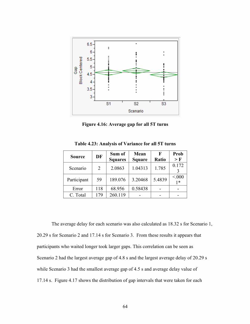
64

Figure 4.16: Average gap for all 5T turns

Table 4.23: Analysis of Variance for all 5T turns

Source DF Sum of

Squares

Mean

Square

F

Ratio

Prob

> F

Scenario 2 2.0863 1.04313 1.785 0.172

3

Participant 59 189.076 3.20468 5.4839 <.000

1*

Error 118 68.956 0.58438 - -

C. Total 179 260.119 - - -

The average delay for each scenario was also calculated as 18.32 s for Scenario 1,

20.29 s for Scenario 2 and 17.14 s for Scenario 3. From these results it appears that

participants who waited longer took larger gaps. This correlation can be seen as

Scenario 2 had the largest average gap of 4.8 s and the largest average delay of 20.29 s

while Scenario 3 had the smallest average gap of 4.5 s and average delay value of

17.14 s. Figure 4.17 shows the distribution of gap intervals that were taken for each

65

scenario. It is evident that Scenario 3 had the smallest average delay as many participants

accepted gaps in the 2nd

or 4th

interval. Scenario 2’s average was heavily influenced by

the people who took the 11th

and 16th

interval experiencing delays of 39.54 s and a max

of 64.5 s as shown in Table 4.23.

Table 4.24: Delay data for all 5T turns

Scenario 1

(16 ft.)

Scenario 2

(14 ft.)

Scenario 3

(12 ft.)

Avg. Delay(s) 18.32 20.29 17.14

Median 20.04 14.04 12.04

Mode 20.04 20.04 5.04

Figure 4.17: Gap interval frequency for 5T turns

0

5

10

15

20

25

30

35

40

45

50

0 (

1.7

7)

1 (

3.2

7)

2 (

3.5

)

3 (

3.5

)

4 (

4.0

)

5 (

4.0

)

6 (

5.0

)

7 (

6.0

)

8 (

4.5

)

9 (

2.0

)

10 (

2.0

)

11 (

7.0

)

12 (

3.0

)

13 (

4.5

)

14 (

4.5

)

15 (

6.0

)

16 (

8.0

)

Inte

rval

Fre

qu

ency


Scenario 1 (16 ft.)

Scenario 2 (14 ft.)

Scenario 3 (12 ft.)

66

Table 4.25: Cumulative delay per traffic interval for 5T turns

Interval Delay

(s)

Gap

(s)

0 0 1.77

1 1.77 3.27

2 5.04 3.5

3 8.54 3.5

4 12.04 4

5 16.04 4

6 20.04 5

7 25.04 6

8 31.04 4.5

9 35.54 2

10 37.54 2

11 39.54 7

12 46.54 3

13 49.54 4.5

14 54.04 4.5

15 58.54 6

16 64.54 8

67

Effects of Age on Gap Acceptance

Throughout the study the participants were defined by two different age groups,

young and middle-old. The young participants were between the ages of 18 and 35 years

old. The middle-old participants were of ages 35 and older. Out of the 60 successful tests

40 participants were young and 20 were in the middle-old category. To evaluate how the

driver age affected gap acceptance various summary statistic were calculated for the two

age groups. As seen in Table 4.24 and 4.25 the younger participants accepted smaller

gaps than those in the middle-old age group. The average gap values were all below 5 s

for the young age group and above 5 s for the middle-old age group. The overall average

for all turns for each age group was 4.82 s for young and 5.23 for the middle-old. Results

from a comparison test confirmed that these two averages were statistically significant

(p=.0002). Similar to the findings of other studies, the older drivers in this simulator

driving experiment tended to drive more conservatively.

Table 4.26: Gap data for young participants

Statistics Scenario 1 Scenario 2 Scenario 3

Avg. Gap (s) 4.87 4.87 4.72

Std. Dev 1.28 1.43 1.30

Mode 4 4 4

Median 5 4.75 4

Table 4.27: Gap data for middle-old participants

Statistics Scenario 1 Scenario 2 Scenario 3

Avg. Gap (s) 5.39 5.30 5.00

Std. Dev 1.39 1.34 1.47

Mode 5 5 6

Median 5 5 5

68

Trajectories

Additional analyses were performed to test how the TWLTL width affected

participants’ ability to maneuver within the TWLTL when they performed their left turn.

For the purpose of this study trajectories were drawn for the second 3T turn for 30

participants. One measurement of maneuverability was based on the number of

encroachments for these 30 participants.

From this data sample there was one encroachment for the 12 ft. TWLTL, two

encroachments for the 14 ft. and 16 ft. TWLTL. After looking at all of the trajectories for

the 12 ft. TWLTL it was apparent that most of the 30 participants stayed within the

middle of the center lane. The participants gravitated more towards the left side of the

lane for the 14 ft. and 16ft. TWLTLs. Trajectories for these TWLTL widths can be seen

in Figure 4.18. From these images it is clear that the variation in lane position and

maneuverability increased as the TWLTL lane width increased. The participants were

more cautious and controlled when turning into the smaller 12 ft. TWLTL width to

prevent any collisions. As the TWLTL width increased the participants tended to utilize

more of the lane width as they made their left turn.

Since there were little discrepancies between the TWLTL widths it is evident that

further analyses and research need to be completed.

69

A (12 ft.) B ( 14 ft.) C (16 ft.)

Figure 4.18: Vehicle trajectories for second 3T turn

70

CHAPTER 5 : DISCUSSION

The purpose of this driving study was to evaluate the effects of different lane and

shoulder width combinations in addition to the effects of different TWLTL widths. Lane

and shoulder width combinations were examined based on lateral position and out of lane

encroachments while maneuverability and gap acceptance were evaluated for the

TWLTLs. The aim of this study is to produce adequate comparisons and

recommendations for engineers and roadway designers regarding which lane, shoulder

and TWLTL widths that can be applied to roadways to improve safety and operation.

Rural Section

In this section the percent time out of lane and number of out of lane

encroachments were evaluated for each lane and shoulder width combination. The

following combinations were 12 ft. lane width and no shoulder, a 12 ft. roadway with a 3

ft. paved shoulder and a 10 ft. roadway with a 2 ft. paved shoulder. There was very little

difference between the two 12 ft. roadway combinations. A total of 5 participants went

out of the lane for the 12 ft. roadway with no shoulder and 7 participants drove out of the

lane for the 12 ft. roadway with a 2 ft. shoulder. A larger difference was seen between

these two combinations when the total number of encroachments was calculated. The 12

ft. roadway with no shoulder had 6 encroachments while the 12 ft. roadway with a 2 ft.

paved shoulder had 13 encroachments. Due to the additional space provided by the

shoulder, participants utilized more of the roadway width. In previous studies it has been

found that the extra space evokes a sense of security and safety as there is more room for

71

error and corrections. Results from the third combination show larger effects due to lane

width. This combination of a 10 ft. roadway with a 2 ft. paved shoulder had a total of 14

participants drive out of the lane boundary with 28 encroachments. These values are

exceeding larger than the results sought from the other two combinations. Due to the

reduction in lane width it was expected that the drivers would have the most difficulty

with this combination. This is also reflected in the average lane position values of -.212

ft. for the 12 ft. roadway with no shoulder, -.100 ft. for the 12 ft. roadway with a 2 ft.

shoulder and .149 ft. for the 10 ft. roadway with a 2 ft. shoulder.

Despite the various encroachments, only one of them exceeded the boundaries of

the shoulder. The numbers of encroachments were also evaluated based on the curve

radii. As expected, the majority of the crossings occurred on the smaller curves that

ranged from 900-1230 ft.

Gap Acceptance

Throughout each scenario gap data was collected for two 3T and 5T left turns.

TWLTL widths of 12, 14 and 16 ft. were tested for 3T and 5T sections. Based on the

average gap many comparisons were made to determine if the TWLTL width had any

effect upon gap acceptance. First, the average gaps for all turns in the 3T sections per

scenario were compared between each other. Results from the analysis found no

significance between any of the scenarios, thus indicating that there was no effect due to

the TWLTL width. Another comparison was made by separating the gap data by the

order in which the scenarios were driven. To be specific, this grouped gap data as every

participants first, second and third scenario driven. These averages were 5.88 s for the

72

first scenario, 5.08 s for the second and 4.90 for the last. Analyses indicated a significant

difference between the first and second scenario and the first and last scenario. This

indicates that the participants drove more cautiously for the first scenario as they were

unaccustomed to the scenario layout and the left turn maneuver into the center lane. As

each scenario had two turns additional comparisons were made to determine if there was

a difference between the first and second turn. These differences were statistically

significant as the majority of the participants accepted smaller gaps for the second turn

than the first. This further indicates that the first turn was used as a learning tool.

The 5T turns were also analyzed separately. The average gaps were 4.5s for the

12 ft. TWLTL, 4.8 s for the 14 ft. TWLTL and 4.6s for the 16 ft. TWLTL. Similar to the

3T results the comparison analysis for the 5T sections revealed no significant difference

between scenarios. Overall, it is apparent that the TWLTL width had no effect upon gap

acceptance. The only effect found was due to the order, first second and third, in which

participants drove.

Trajectories

Throughout the study the participants performed various left turn maneuvers on a

3T and 5T roadway. For this study, vehicle trajectories were drawn for 30 participants’

second 3T turn in each scenario. The results were inconclusive regarding the effect that

the TWLTL width had on the drivers’ maneuverability as they turned into the TWLTL.

Based on the trajectories there was one encroachment for the 12 ft. TWLTL with and two

encroachments for the 14ft. and 16 ft. TWLTL widths. Additional analyses regarding the

73

remaining turns for all participants will need to be evaluated to further determine effects

caused by the TWLTL width.

Age Comparison

Driver characteristics pertaining to age was also tested in relationship to gap

acceptance. Results found that for each scenario the average gap for older participants

was higher than the average gap for younger participants. The overall averages of 4.82 s

for young and 5.23 s for the older participants were found to be statistically significant.

Similar to Yan et al’s, study, these results found that older drivers, driver more

conservatively.

74

CHAPTER 6 : CONCLUSION

The main goal of this study is to determine the influence that flexible lane width

standards have on the safety and operation of roadways in South Carolina. After the

completion of the field studies in Part 1 of this study it was apparent that to further

investigate the effects of lane width a driving simulator study needed to take place.

Before commencing the study an extensive literature review was completed to gain

knowledge on previous driving simulator studies and to aid in the design of this study.

Immense care was taken during the development of the custom design to ensure that

sufficient comparative research regarding the SCDOT’s inquiries was implemented

throughout the study. Based on the findings of this comparative research additional

comments and recommendations can be drawn regarding the ultimate goal of using

flexible lane width standards in South Carolina.

Recommendations

A major portion of this study involved the evaluation of different lane and

shoulder width combinations on a rural two-lane highway with a design speed of 50 miles

per hour. Results from this section of the study found very little difference between the

12 ft. roadway with no paved shoulder and the 12 ft. roadway with a 2ft. paved shoulder.

A total of 5 out of 60 participants drove out of the lane for the 12 ft. roadway with no

paved shoulder and 7 out of 60 participants drove out of the lane for the 12 ft. roadway

with a 2 ft. paved shoulder. The total number of encroachments were 6 and 13

respectively. These combinations were also compared to a 10 ft. roadway with a 2 ft.

75

paved shoulder. This lane width had a larger effect upon drivers as 14 participants drove

out of the lane during this roadway section with a total of 30 encroachments. Most of the

encroachments took place along the curves of the roadway. The number and magnitude

of these encroachments for each combination is show in Table 6.1.

Table 6.1: Magnitude of encroachments

Direction Left Right

Magnitude (ft.) < .5 ft. .51-1 ft. >1 ft. < .5 ft. .51-1

ft. >1 ft.

Scenario 1 (12 ft. - 0 ft.) 3 2 0 1 0 0

Scenario 2 (12 ft. - 2 ft.) 4 2 1 4 (1)* 1 1

Scenario 3 (10 ft. - 2 ft.) 11 3 0 12 (2)* 4 0

*Number in parenthesis is an encroachment along a straight section

Even though the 10 ft. roadway had more encroachments, none of the right hand

crossings exceeded the boundaries of the shoulder. No roadside encroachments occurred

for the two scenarios in which a shoulder was present. This can be seen in Table 6.1 as

the majority of encroachments for all scenarios were within half of a foot. As there was

no shoulder in Scenario 1, there was only one roadside encroachment. From this

perspective there was no major difference between the three lane and shoulder width

combinations. These results also support the Highway Safety Manual as there is only a

0.2 total crash per mile difference between the three combinations tested in the driving

simulator.

76

Table 6.2: Highway Safety Manual combination comparison

These findings further encourage the recommendation made by Part 1 regarding

the safety and use of 10-12 ft. lane widths for rural two-lane roadways. Comparisons

between the SCDOT’s existing HDM guidelines and recommendations made based on

Part 1 of this research can be seen in Table 6.3. The full table can be seen in Appendix G.

From the table it is evident that the SCDOT’s HDM primarily uses a 12 ft. lane

width for rural two- lane arterials and a range of 11-12 ft. for rural two-lane collectors.

Results from Part 1 of the research encourage the use of AASHTO standards that include

11 to 12 ft. lane widths for rural two-lane arterials and 10 to 12 ft. lane widths for rural

two-lane collectors. Findings from the simulator study also encourage the use of 10 to 12

ft. lane widths on rural two- lane roadways in South Carolina. Recommendations from

Part 1, also advised that a 10 ft. lane width only be used on a roadway with a speed limit

of 40 miles per hour or less. Results from the simulator study agree with this

recommendation as a larger effect due to the narrower lane width was seen at a 50 miles

per hour speed limit. As there was a high of 30 encroachments for the 10 ft. roadway, it is

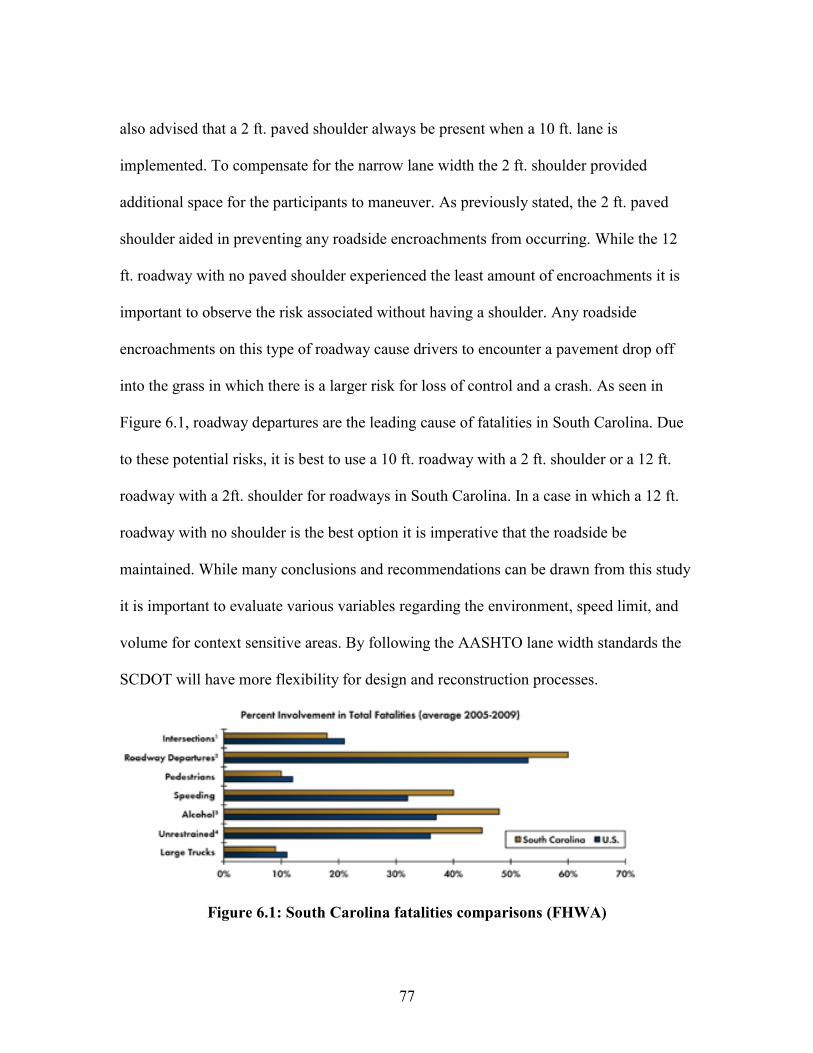
77

also advised that a 2 ft. paved shoulder always be present when a 10 ft. lane is

implemented. To compensate for the narrow lane width the 2 ft. shoulder provided

additional space for the participants to maneuver. As previously stated, the 2 ft. paved

shoulder aided in preventing any roadside encroachments from occurring. While the 12

ft. roadway with no paved shoulder experienced the least amount of encroachments it is

important to observe the risk associated without having a shoulder. Any roadside

encroachments on this type of roadway cause drivers to encounter a pavement drop off

into the grass in which there is a larger risk for loss of control and a crash. As seen in

Figure 6.1, roadway departures are the leading cause of fatalities in South Carolina. Due

to these potential risks, it is best to use a 10 ft. roadway with a 2 ft. shoulder or a 12 ft.

roadway with a 2ft. shoulder for roadways in South Carolina. In a case in which a 12 ft.

roadway with no shoulder is the best option it is imperative that the roadside be

maintained. While many conclusions and recommendations can be drawn from this study

it is important to evaluate various variables regarding the environment, speed limit, and

volume for context sensitive areas. By following the AASHTO lane width standards the

SCDOT will have more flexibility for design and reconstruction processes.

Figure 6.1: South Carolina fatalities comparisons (FHWA)

78

Table 6.3: Part 1 recommendations

Functional

Class

SCDOT

HDM

Reference

Variable Existing

Values

in HDM

Summary

of

Proposed

Changes

Basis for

proposed HDM

change

Rural Two-

Lane

Arterials

Fig. 20.1A Traveled

Way Width

24 ft. 22-24 ft. Research results,

AASHTO, other

DOT’s, Harwood

et al, 2000

Rural Two-

Lane

Collectors

Fig. 20.1B Traveled

Way Width

22-24 ft. 20-24 ft. Research results,

AASHTO, other

DOT’s, Harwood

et al, 2000

Rural Two-

Lane

Arterials

Fig. 20.1D,

Footnote 1

(HDM

13.2.3)

Travel Lane

Width

12 ft. 11-12 ft.

(see

criteria in

Table 5.3)

Research results,

AASHTO, other

DOT’s, Harwood

et al, 2000

Rural Two-

Lane

Arterials

Fig. 20.1D

(HDM

13.2.5)

Aux. Lane

Width

12 ft. 11-12 ft.

(see

criteria in

Table 5.4)

AASHTO, other

DOT’s

Rural Two-

Lane

Arterials

Fig. 20.1D

(HDM

21.2.7)

TWLTL

Lane

Width


AASHTO, other

DOT’s, Fattis et

al, 2010

Rural Two-

Lane

Collectors

Fig. 20.1E,

Footnote 1

(HDM

13.2.3)

Travel Lane

Width

11-12 ft. 10-12 ft.

(see

criteria in

Table 5.5)

Research results,

AASHTO, other

DOT’s, Harwood

et al, 2000

Rural Two-

Lane

Collectors

Fig. 20.1E

(HDM

13.2.5)

Aux. Lane

Width

11-12 ft. 10-12 ft.

(see

criteria

Table 5.4)

AASHTO, other

DOT’s

Rural Two-

Lane

Collectors

Fig. 20.1E

(HDM

21.2.7)

TWLTL

Lane

Width


AASHTO, other

DOT’s, Gattis et

al, 2010

79

Additional analyses from the simulator study were performed to determine

the effects of TWLTL width on gap acceptance and on turning vehicle encroachments

into through lanes. Several ANOVA tests found that the tested TWLTL widths of 12 ft.,

14ft. and 16 ft. had no effect upon gap acceptance for the 3T and 5T sections.

Trajectories were drawn for 30 participants’ second 3T turn to evaluate the effect

TWLTL width had on vehicle encroachments into through lanes. Moreover, these results

found very little difference between the three widths of 12, 14 and 16 ft. The results

defied the prediction that more encroachments would occur in the smaller lane width of

12 ft. For the 30 participants there was one encroachment for the 12 ft. TWLTL and two

encroachments for the 14 ft. and 16 ft. TWLTL widths. More lane position variation was

found for the larger TWLTL widths as participants took advantage of the larger space for

maneuvering. Based on these findings it is recommended that 12, 14 and 16 ft. TWLTL

widths can be used in South Carolina. Currently the SCDOT HDM uses 15 ft. TWLTL

widths. As there were no major differences in driver behavior for the TWLTL widths

tested in the simulator it is recommended that 12 to 16 ft. TWLTL widths can be used in

South Carolina. To further investigate any variation between the widths further analyses

should be conducted for the remaining turns in the scenarios.

As previously stated, field studies were conducted in 2011 to evaluate the effect

different roadway combinations and TWLTL widths had on driver behavior. Due to the

limited sample size of roadways with specific attributes from these studies additional

research needed to take place. By using the driving simulator our research team was able

to directly focus on context sensitive roadways in South Carolina. From the simulator

80

results, additional evidence was provided backing up the recommendations made from

the field studies in Part 1. The combined results from both studies indicated that lane

widths of 10 to 12 ft. were acceptable for rural two-lane roadways in South Carolina. The

simulator study also found that specific combinations of a 12 ft. roadway with no

shoulder, 12 ft. roadway with a 2ft. shoulder and a 10 ft. roadway with a 2 ft. shoulder.

Additional results from both studies found that 12 to 16 ft. TWLTL widths were

acceptable. Together, results from the field and simulator study succeeded in

recommending flexible lane width standards for the SCDOT.

81

APPENDIX A

Traffic Intervals

3T

[ "1.5" "3.5" "3.5" "4.0" "4.0" "5.0" "6.0" "4.5" "7.0" "3.0" "4.5" "4.5" "6.0" "8.0" "4.5"

"5.0" "6.0" "4.0" "7.0" "4.5" "4.0" "5.0" "3.5" "4.0" "5.0" "3.0" "3.5" "3.5" "4.0" "4.0"

"5.0" "6.0" "4.5" "7.0" "3.0" "4.5" "4.5" "6.0" "8.0" "4.5" "5.0" "6.0" "4.0" "7.0" "4.5"

"4.0" "5.0" "3.5" "4.0" "5.0"]

5T

Left Lane [ "1.5" "7.0" "8.0" "11.0" "6.5" "7.0" "7.5" "10.5" "12.5" "11.0" "11.0" "8.5"

"8.5" "9.0" "8.5" "8.5" "10.0" "6.5" "9.5" "8.0" "10.5" "9.0" "8.0" "10.5" "10.0" "13.0"

"7.0" "3.0" "7.0" "8.0" "11.0" "11.5" "7.5" "10.5" "12.5" "11.0" "11.0" "8.5" "8.5" "9.0"

"8.5" "8.5" "10.0" "6.5" "9.5" "8.0" "10.5" "9.0" "8.0" "10.5" "10.0"]

Right Lane [list "5.0" "7.5" "9.0" "10.5" "2.0" "10.0" "9.0" "14.0" "9.5" "10.0" "11.5"

"9.0" "7.5" "10.0" "7.0" "11.0" "7.0" "7.5" "9.0" "10.0" "11.0" "6.5" "10.0" "10.0" "11.5"

"11.0" "2.5" "6.5" "7.5" "9.0" "10.5" "10.0" "9.0" "14.0" "9.5" "10.0" "11.5" "9.0" "7.5"

"10.0" "7.0" "11.0" "7.0" "7.5" "9.0" "10.0" "11.0" "6.5" "10.0" "10.0" "11.5"]

5T Effective Gaps

[list "3.27" "3.5" "3.5" "4.0" "4.0" "5.0" "6.0" "4.5" "2.0" "2.0" "7.0" "3.0" "4.5" "4.5"

"6.0" "8.0" "4.5" "5.0" "6.0" "4.0" "7.0" "4.5" "4.0" "5.0" "3.5" "4.0" "5.0" "5.0" "3.5"

"3.5" "5.0" "6.0" "4.0" "3.0" "3.5" "4.0" "5.5" "3.5" "4.5" "5.5" "5.0" "6.0" "3.0" "3.5"

"4.5" "5.5" "5.0" "5.0" "5.0" "6.5"]

82

APPENDIX B

Curve Boundaries

Scenario 1 and 2

Straight 1

Curve 3

Start End

Start End

x 2701.5 2702.1

x 2730 2708.6

y 14700.9 15195.4

y 14010.4 14134.3

z 4 0

z 10 13.4

Curve 1

Straight 4

Start End

Start End

x 2677.8 2702.2

x 2731.8 2730.1

y 14534.7 14683.5

y 13784.2 13984.8

z 6 4

z 7.4 10.2

Curve 2

Curve 4

Start End

Start End

x 2656.9 2661.3

x 2713.6 2732.5

y 14272 14488.6

y 13615 13758.9

z 14.5 6

z 0.2 6.6

Straight 3

Straight 5

Start End

Start End

x 2701.5 2663.1

x 2661.2 2707

y 14155 14254.1

y 13476.8 13597.1

z 14 14.9

z -2 -0.2

Curve 5

Curve 6

Start End

Start End

x 2642.5 2652.4

x 2688.4 2680.3

y 13261.1 13453.3

y 13005.4 13122.3

z 1.7 -1.9

z 8.3 4

83

Straight 6

Curve 7

Start End

Start End

x 2671.8 2649.9

x 2701.8 2677.4

y 13154.4 13233.9

y 12737.7 12899.5

z 3 2

z 12.2 9

Scenario 3

Straight 13

Curve 12

Start End

Start End

x 2701.7 2701.7

x 2715.3 2751.5

y 15047.8 15195.9

y 14377.5 14596.7

z 0 0

z 10.6 8.1

Curve 13

Curve 11

Start End

Start End

x 2716.3 2701.7

x 2667.4 2668.9

y 14814.2 15018.8

y 13996.8 14297.2

z 0 0

z 0.5 7.7

Straight 12

Straight 10

Start End

Start End

x 2748.5 2721.7

x 2715.6 2673.9

y 14616 14780.2

y 13910.9 13985.3

z 7.3 0

z 0 0.3

84

Curve 10

Straight 8

Start End

Start End

x 2736.8 2725

x 2693.9 2669.6

y 13618.4 13892.8

y 13044.9 13291

z 8.4 0.1

z 15.8 19

Curve 9

Curve 8

Start End

Start End

x 2667.4 2687.6

x 2697.2 2697.6

y 13315.9 13493.1

y 12810.1 13011.7

z 19 15.3

z 13.7 15.4

85

APPENDIX C

Script to Conduct Experiment

Note: During transitions between sessions it is important NOT to say things such as “good job”, “bad job”, or anything of this reinforcing nature Pre-participant

Consent Form

Motion Sickness Forms

Make sure puke can is by car and empty

Sim Data Forms Welcome—if you have a cell phone please make sure it is turned off before we begin. Please note that I will be reading from a script throughout the experiment, and I may not be able to answer certain questions that pertain to the experiment until after we have completed the study.

Place experiment in progress sign on door.

Thank you for choosing to participate in our study. Before we get started please read and sign this consent form. Should you have any questions, please feel free to ask. After you have read it, please initial the bottom of the pages and sign and date the back page. If you would like a copy of the signed consent form for your records, just let me know.

The purpose of this study is to investigate driving behavior in various settings.

Before we get started I am going to ask you some motion sickness questions. I will ask you these same questions after each time you drive today. If you feel uncomfortable at any time during the experiment, please let me know immediately.

Before we get started we will also be taking a few minutes to take your blood pressure.

86

Ask Motion Sickness Questionnaire and Demographics questions

Take blood pressure as they are doing the questions

You may now get into the car.

Please sit in the vehicle and move the seat forward or backward so that it suits you.

Show car controls

The controls work just like a regular automatic transmission vehicle: the gas is on the right, and the brake is on the left. The car should already be in park, so please do not change gears as the car is already in drive.

The steering is quite loose and sensitive, meaning the vehicle reacts as if it has too much power steering.

You will now have several practice sessions to get used to the vehicle and the simulator.

Once you see the road you may start driving. Your goal for today will be to drive through the scenarios as you would in your own vehicle.

If you start to feel uncomfortable or uneasy at any time please tell me immediately.

I will tell you when to begin each scenario.

Load “1LaneKeeping_Straight” Enter participant number then “#_LWst”

For your first practice session:

(Please wait for instructions screen-Press A Scenario shows up) You will drive on a straight road to familiarize yourself with the vehicle for two 30 second periods.

( Press A- Dots show up) On the screen you can see five dots. These dots will tell you where you are in the lane to help you get a feel for the car.

(Press A) The green dot appears if you are in the middle of the road.

87

(Press A) This yellow dot indicates that you are driving in the left side of the lane.

(Press A) The red dot shows that you are out of the lane.

(Press A twice) This yellow dot indicates that you are driving along the right edge of the lane.

(Press A) This red dot shows you are out of the lane to the right. (Press A) All red dots show that you are completely out of the lane.”

(Press A twice) For the first run you can drive at any speed that you feel comfortable. The scenario will cut off in 30 sec. Please move around inside the lane until you are comfortable with the lane’s boundaries.

(Press A) Now you will get to drive this scenario again for another 30 sec. This time try to maintain the 45 mph speed limit. (Set timer for 30 sec) A voice will also instruct you to slow down if you drive faster than 45 miles per hour. When my timer goes off , lift your foot off the gas, and I will turn off the driving simulator. You may now begin.

You can repeat practice sessions as many times as necessary to feel comfortable.

Buzz timer after 30 seconds, wait for them to lift foot off of gas and stop scenario

Collect Data for this Practice Session

Ask Motion Sickness Questions- Record on Data Sheet

Load “3.Lane Keeping_Curves_DS600” Enter participant number then “#_LWcu”

For your second practice session

(Please wait for instructions screen-Press A) Now you will practice staying in your lane on a continuously curvy road. It is designed to be difficult for everyone as it is intentionally quite curvy. This time you will not have the dots to show you where you are in the lane.

88

A voice will also instruct you to slow down if you drive faster than 50 miles per hour.

This session will automatically end after you maintained lane position for a minute. When the screen goes black, lift your foot off the gas, and I will turn off the driving simulator.

You can repeat each practice session as many times as necessary to feel comfortable. (Press A-Car starts) You may begin now.

At the top of the left screen record the number of Departures in the data sheet

Wait for them to lift foot off of gas and stop scenario


Ask Motion Sickness Questions- Record on Data Sheet Take a break. Get participant out of car. Offer restroom break.

Load “5.Stopping_DS600” Enter participant number then “#_LWstop”

For your third practice session

(Please wait for instructions screen) -You will practice stopping. (Press A- Scenario shows up) For this scenario you will have to do 5 complete stops at a series of stop signs and lights. A voice will tell you to slow down if you drive faster than the posted speed limit. Throughout the scenario you will only drive straight. After each stop proceed through the intersection.

(Press A-car starts up) You may now begin

(On the left screen you can see how far the subject gets to the stop bar line, negative means behind the line, positive is they are past the stop bar-record these values in data sheet)

(After they go through last intersection)You have now completed 5 stops so go ahead and stop the car and place it in park. (Stop the scenario)



89

Ask Motion Sickness Questions- Record on Data Sheet Make participant get out of car. Offer restroom break. (They

must get out after this scenario Load “6.Left turns_DS600” Enter participant number then #_LWleft”

For your fourth practice session

(Please wait for instructions screen) –Now you will practice making left turns.

(Press A- Scenario shows up) For this scenario you will make 6 left turns. For the first turn the simulator will control your speed in order to show you how to do a left turn. While this is happening you will need to push on the gas.

A voice will tell you to slow down if you drive faster than the posted speed limit. At the end when the screen goes black put the car in park.

(Press A- Start car) You may now begin.

(On the left screen you can see the number of left turns the subject has made) --the scenario will automatically turn black when they have completed all turns



Ask Motion Sickness Questions- Record on Data Sheet Take a break. Get participant out of car. Offer restroom break.

Load “7.Right Turns_DS600” Enter participant number then “#_LWright”

For your fifth and final practice session

(Please wait for instructions screen-Press A)You will practice making right turns. For this scenario there will be a total of 4 right turns. For the first turn the simulator will control your speed

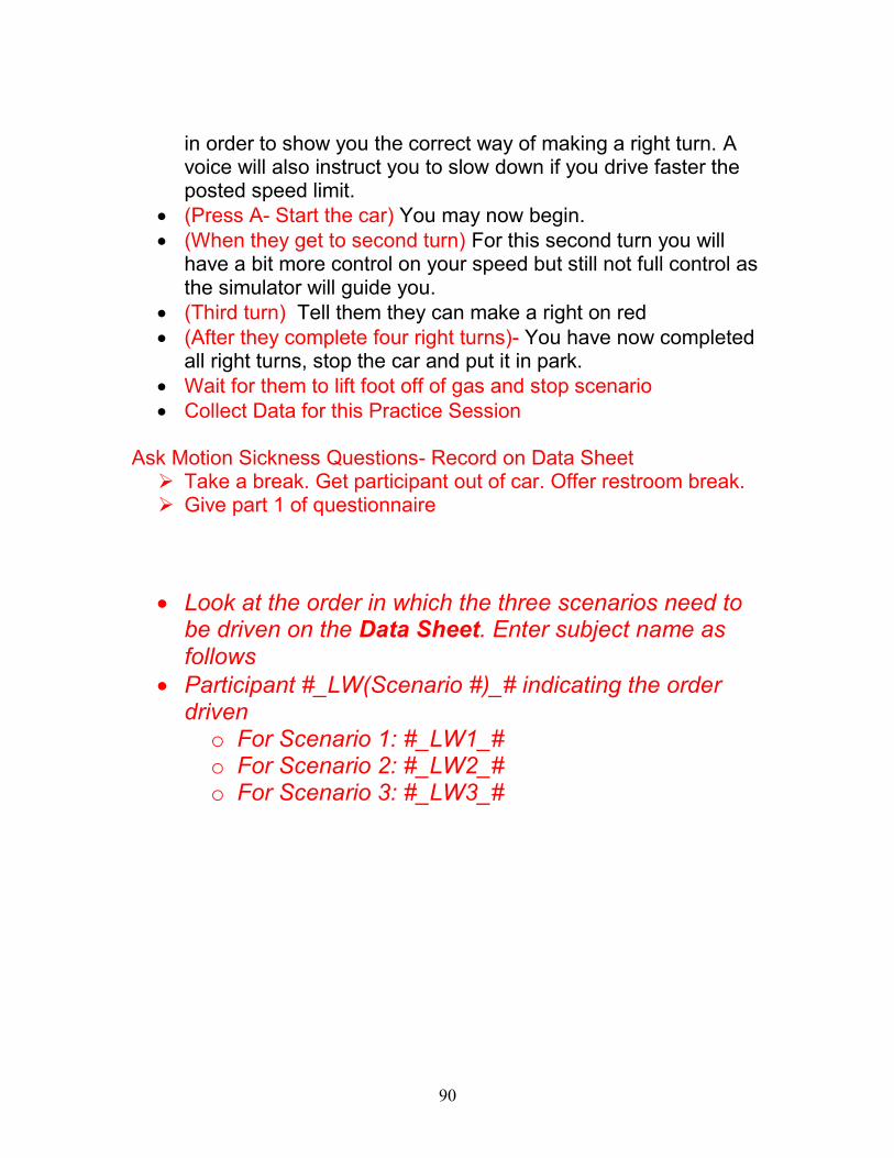
90

in order to show you the correct way of making a right turn. A voice will also instruct you to slow down if you drive faster the posted speed limit.

(Press A- Start the car) You may now begin.

(When they get to second turn) For this second turn you will have a bit more control on your speed but still not full control as the simulator will guide you.

(Third turn) Tell them they can make a right on red

(After they complete four right turns)- You have now completed all right turns, stop the car and put it in park.


Collect Data for this Practice Session Ask Motion Sickness Questions- Record on Data Sheet Take a break. Get participant out of car. Offer restroom break. Give part 1 of questionnaire

Look at the order in which the three scenarios need to be driven on the Data Sheet. Enter subject name as follows

Participant #_LW(Scenario #)_# indicating the order driven o For Scenario 1: #_LW1_# o For Scenario 2: #_LW2_# o For Scenario 3: #_LW3_#

91

CONDITION 1 Load “LaneWidth_#” Enter participant number then “#_LW#_1”

Now that you have completed the practice sessions, we will begin the actual study. It is important that you drive as you would in your own vehicle. In the beginning of the scenario try to maintain the posted speed limit. A voice will tell you if you are going too fast or too slow. Throughout the scenario you will also be doing a series of left turns. For these turns, turn left into the two way left turn lane and stop until all cars on your right have passed. Please be sure to listen to all of the voice commands in the simulator. This scenario should take about 10 minutes. You may now begin. Ask Motion Sickness Questions- Record on Data Sheet Make participant get out of car Offer snack Complete part 2 of questionnaire


It is important that you drive as you would in your own vehicle. In the beginning of the scenario try to maintain the posted speed limit. A voice will tell you if you are going too fast or too slow. Throughout the scenario you will also be doing a series of left turns. For these turns, turn left into the two way left turn lane and stop until all cars on your right have passed. Please be sure to listen to all of the voice commands in the simulator. This scenario should take about 10 minutes. You may now begin.

92

Ask Motion Sickness Questions-Record on Data Sheet Make participant get out of car Complete part 3 of Questionnaire Measure Blood Pressure


It is important that you drive as you would in your own vehicle. In the beginning of the scenario try to maintain the posted speed limit. A voice will tell you if you are going too fast or too slow. Throughout the scenario you will also be doing a series of left turns. For these turns, turn left into the two way left turn lane and stop until all cars on your right have passed. Please be sure to listen to all of the voice commands in the simulator. This scenario should take about 10 minutes. You may now begin.

- Ask Motion Sickness Questions-Record on Data Sheet - Have person get out of car and sit at table

o Ask “what do you think was the purpose of this study?” o Ask post questions on page 4 of Data Sheet o Take Blood Pressure

- Pay participant Thank you for participating in this research study

Remember that the purpose of the study was to investigate driving behavior in various settings.

Complete Master subject list “success” column now.

Email [email protected] with attendance/success information.

Backup data to external hard drive

93

APPENDIX D

Participant Data Sheets

Participant Number: _______________

Date: _______________

Experimenter: _______________________

Did you give participant their copy of the consent form? Yes or No

Did you file the signed consent form? Yes or No

Ask prior to running experiment:

Do you have a valid US driver’s license? ______________

Age _______

Age Group – Young (18-34) / Middle (35- 65) / Old (65+)

Gender _______

Years driving ____

Are you a resident of SC? Yes / no

Do you have a past history of motion sickness?__________

Do you have a past history of migraines?________

Do you have any vision problems?_________

94

Participant Number:

Perform Blood Pressure Test ______ ______ ______ ______ ______

Completed Scenarios

Nausea Questions

Answer each question on a scale from 0 to 10 where 0 is “not at all”

and 10 is “severely.” Comments

Sick to your

stomach Sweaty

Light

headed Nauseous Hot/warm Dizzy

1.) Straight

2.) Curvy

Edge touches

________

3.)Stopping

Distance to stop bar

1.) _____

2.) _____

3.) _____

4.) _____

5.) _____

4.) Left Turns

5.) Right Turns

Questionnaire

95

Participant Number:

Completed Scenarios

Nausea Questions

Answer each question on a scale from 0 to 10 where 0 is “not at

all” and 10 is “severely.” Comments

Sick to your

stomach Sweaty

Light

headed Nauseous Hot/warm Dizzy

LaneWidth_1

______

Questionnaire

LaneWidth_2

______

Questionnaire

LaneWidth_3

______

Perform Blood Pressure Test ______ ______ ______ ______ ______

Ask Purpose of the study

Fill out master subject list

Email status to Brian: [email protected]

96

Participant Number: _______________

Ask at end of experiment:

Estimate the number of miles you drive each year _______

How many days do you drive each week _______

What kind of vehicle do you drive? Make____ Model____ Year ____

Have you been in a crash in the last year while driving? Yes / no

Have you been in a crash in the last 5 years while driving? Yes / no

Were you considered at fault in any of these crashes? Yes / no

If Yes, how many? _____

Have you received a speeding ticket in the last year? Yes / no

Have you received a speeding ticket in the last 5 years? Yes / no

Do you typically wear your seatbelt? Yes / no

Do you ever talk on your cell phone when you drive? yes / no

Do you ever text message when you drive? Yes / no

97

APPENDIX E

Participant Data

Participant #

Age

Group Completed

1 Young Yes

2 Young Yes

3 Young Yes

4 Young No- Sim sick

5 Young Yes

6 Middle Yes

7 Young Yes

8 Young Yes

9 Young Yes

10 Young Yes

11 Young Yes

12 Young Yes

13 Middle Yes

14 Young Yes

15 Young Yes

16 Young Yes

17 Young Yes



20 Young Yes

21 Young Yes

22 Young Yes

24 Young Yes

25 Young Yes



27 Young Yes

28 Young Yes

29 Young Yes

30 Young Yes

98

31 Young Yes

32 Young Yes

33 Middle Yes

34 Middle Yes

35 Young Yes

36 Middle Yes

37 Middle No- Sim sick

38 Middle Yes-Little sick

39 Young Yes

40 Young Yes

41 Young Yes

42 Young Yes

43 Young Yes

44 Middle Yes


46 Young Yes

47 Young Yes

48 Middle Yes

49 Middle Yes

50 Middle Yes

51 Young Yes

52 Young Yes


54 Young Yes

55 Middle Yes



58 Middle Yes

59 Young Yes

60 Middle Yes

61 Middle Yes

62 Middle Yes

63 Middle Yes

64 Middle Yes

65 Middle Yes

66 Middle Yes

99

67 Middle No

68 Young Yes


70 Middle Yes

71 Young Yes

72 Young Yes

100

APPENDIX F

Post Question Results on Driving Behavior

Estimate the number of miles you drive each year

How many days do you drive each week?

Age group Avg. Age Avg. Yrs Driving Avg. Miles/ Yr

Young 21 5.5 11000

Middle/Old 49 31.5 14000

Have you been in a crash in the last year (5 years) while driving?

Age group Crash -1 yr Crash-5 yr

Young 2 10

Middle/Old 1 6

Have you received a speeding ticket in the last year (5 years)?

Age group Ticket -1 yr Ticket-5 yr

Young 13 26

Middle/Old 1 6

Do you talk on your cell phone while driving?

Cell Phone Young Middle/Old

Yes 32 12

No 8 8

Do you text message while driving?

Text

Messaging Young Middle/Old

Yes 11 4

No 29 16

101

APPENDIX G

Recommendations

Table 5.1: Summary of Proposed SCDOT HDM Changes for Rural Arterials and

Collectors

Functional

Class

SCDOT

HDM

Reference

Variable Existing

Values

in HDM

Summary

of

Proposed

Changes

Basis for

proposed HDM

change

Rural Two-

Lane

Arterials

Fig. 20.1A Traveled

Way Width


AASHTO, other

DOT’s, Harwood

et al, 2000

Rural Two-

Lane

Collectors

Fig. 20.1B Traveled

Way Width

22-24 ft. 20-24 ft. Research results,

AASHTO, other

DOT’s, Harwood

et al, 2000

Rural Two-

Lane

Arterials

Fig. 20.1D,

Footnote 1

(HDM

13.2.3)

Travel Lane

Width

12 ft. 11-12 ft.

(see

criteria in

Table 5.3)

Research results,

AASHTO, other

DOT’s, Harwood

et al, 2000

Rural Two-

Lane

Arterials

Fig. 20.1D

(HDM

13.2.5)

Aux. Lane

Width

12 ft. 11-12 ft.

(see

criteria in

Table 5.4)

AASHTO, other

DOT’s

Rural Two-

Lane

Arterials

Fig. 20.1D

(HDM

21.2.7)

TWLTL

Lane

Width


AASHTO, other

DOT’s, Fattis et

al, 2010

Rural Two-

Lane

Collectors

Fig. 20.1E,

Footnote 1

(HDM

13.2.3)

Travel Lane

Width

11-12 ft. 10-12 ft.

(see

criteria in

Table 5.5)

Research results,

AASHTO, other

DOT’s, Harwood

et al, 2000

Rural Two-

Lane

Collectors

Fig. 20.1E

(HDM

13.2.5)

Aux. Lane

Width

11-12 ft. 10-12 ft.

(see

criteria

Table 5.4)

AASHTO, other

DOT’s

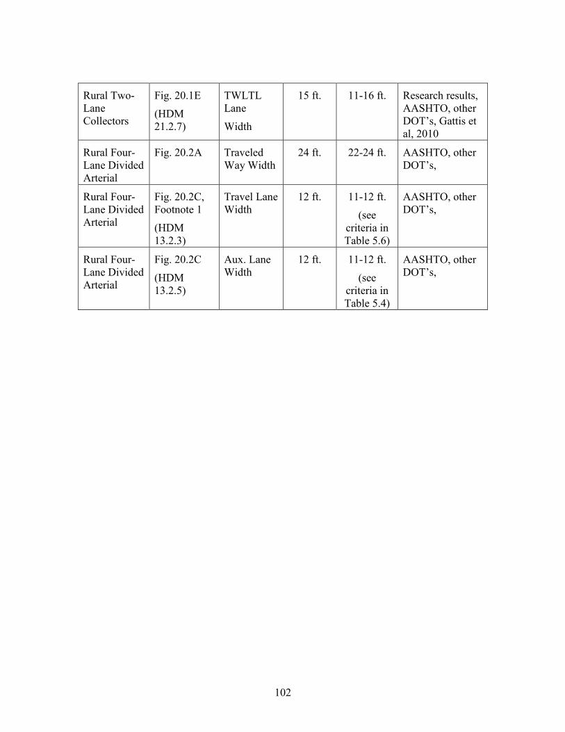
102

Rural Two-

Lane

Collectors

Fig. 20.1E

(HDM

21.2.7)

TWLTL

Lane

Width


AASHTO, other

DOT’s, Gattis et

al, 2010

Rural Four-

Lane Divided

Arterial

Fig. 20.2A Traveled

Way Width

24 ft. 22-24 ft. AASHTO, other

DOT’s,

Rural Four-

Lane Divided

Arterial

Fig. 20.2C,

Footnote 1

(HDM

13.2.3)

Travel Lane

Width

12 ft. 11-12 ft.

(see

criteria in

Table 5.6)

AASHTO, other

DOT’s,

Rural Four-

Lane Divided

Arterial

Fig. 20.2C

(HDM

13.2.5)

Aux. Lane

Width

12 ft. 11-12 ft.

(see

criteria in

Table 5.4)

AASHTO, other

DOT’s,

103

Table 5.2: Summary of Proposed SCDOT HDM Changes for Urban/Suburban Arterials

and Collectors

Functional

Class

SCDOT

HDM

Reference

Variable Existin

g

Values

in

HDM

Summary

of Proposed

Changes

Basis for

proposed

HDM change

Four-Lane

Suburban/Urba

n Street

Fig. 21.2A Traveled

Way

Width

24 ft. 22-24 ft. Research

results,

AASHTO,

other DOT’s,

Potts et al,

2007, Mbatta et

al, 2012

Five-Lane

Urban Street

(with

Shoulders)

Fig. 21.2B Traveled

Way

Width


results,

AASHTO,

other DOT’s,

Potts et al,

2007, Mbatta et

al, 2012

Five-Lane

Urban Street

(with

Shoulders)

Fig. 21.2B

(HDM

21.2.7.2)

TWLTL

Lane

Width


results,

AASHTO,

other DOT’s,

Gattis et al,

2010

Five-Lane

Urban Street

(Curb and

Gutter)

Fig. 21.2C Traveled

Way

Width


results,

AASHTO,

other DOT’s,

Potts et al,

2007, Mbatta et

al, 2012

Five-Lane

Urban Street

(Curb and

Gutter)

Fig. 21.2C

(HDM

21.2.7.2)

TWLTL

Lane

Width


results,

AASHTO,

other DOT’s,

Gattis et al,

2010

104

Suburban/Urba

n Multilane

Arterials

Fig. 21.3A

(HDM 9.2)

(HDM

13.2.3)

Travel

Lane

Width

12 ft. 11-12 ft.

(see criteria

in Table

5.7)

Research

results,

AASHTO,

other DOT’s,

Potts et al,

2007, Mbatta et

al, 2012

Suburban/Urba

n Multilane

Arterials

Fig. 21.3A

(HDM

21.2.7.2)

TWLTL

Lane

Width


results,

AASHTO,

other DOT’s,

Gattis et al,

2010

Suburban/Urba

n Collectors

Fig. 20.1E

(HDM 9.2)

(HDM

13.2.3)

Travel

Lane

Width

12 ft. 11-12 ft.

(see criteria

in Table

5.8)

Research

results,

AASHTO,

other DOT’s,

Potts et al,

2007, Mbatta et

al, 2012

Suburban/Urba

n Collectors

Fig. 20.1E

(HDM

21.2.7.2)

TWLTL

Lane

Width


results,

AASHTO,

other DOT’s,

Gattis et al,

2010

Rural Four-

Lane Divided

Arterial

Fig. 20.2C,

Footnote 1

(HDM

13.2.3)

Travel

Lane

Width

12 ft. 11-12 ft.

(see criteria

in Table

5.6)

AASHTO,

other DOT’s,

Rural Four-

Lane Divided

Arterial

Fig. 20.2C

(HDM

13.2.5)

Aux. Lane

Width

12 ft. 11-12 ft.

(see criteria

in Table

5.4)

AASHTO,

other DOT’s,

Table 5.3: Proposed Travel Lane Width Criteria for Rural Two-Lane Arterials

Travel Lane Width (*) Criteria and Conditions

11 ft. min., 12 ft. Design Speed 55 mph or less, assuming a 2 ft. paved

105

desirable shoulder, if shoulder width does not meet minimum requirements, use 12 ft. min

12 ft. min. Design Speed 60 mph or greater

Footnotes:

1. If lower design speeds are allowed, narrower travel lane widths could be acceptable, 10 ft. min.

2. For industrial areas or locations with higher heavy vehicle use, 12 ft. lanes should be used.

3. Criteria for Travel Lane Width assumes no problematic prior crash histories related to lane width including run off the road, sideswipe (same and opposite direction), head-on crashes.

4. Under no condition should travel lane widths be less than 10 ft. min.

Table 5.4: Proposed Auxiliary Lane Width Criteria for Rural Two-Lane Arterials

Auxiliary Lane Width (*) Criteria and Conditions

10 ft. min., 12 desirable Design Speed of 35 mph or less

11 ft. min., 12 ft. desirable

Design Speed greater than 35 mph and 55 mph, or less


Footnotes:



Table 5.5: Proposed Travel Lane Width Criteria for Rural Two-Lane Collectors

Travel Lane Width (1) Criteria and Conditions

10 ft. min. AADT less than 400 veh./day, design speed 40mph or less, 2ft. paved shoulder required

11 ft. min. AADT between 401-2000 veh./day, design speed 50mph or less, assuming a 2 ft. paved shoulder, if shoulder width does not meet minimum requirements, use 12 ft. min

12 ft. min. AADT over 2,000, design speed 60 mph or greater

106

Footnotes:





Table 5.6: Proposed Travel Lane Width Criteria for Rural Multilane Arterials



AADT less than 4,000 veh./day, Design Speed 55 mph or less, assuming a 2 ft. paved shoulders, if shoulder width does not meet minimum requirements, use 12 ft. min

12 ft. min. AADT greater than 4,000 veh./day, Design Speed 60 mph or greater, assuming a 2 ft. paved shoulders

Footnotes:





Table 5.7: Proposed Travel Lane Width Criteria for Suburban/Urban Multilane Arterials

and Collectors


10 ft min, 12 ft desirable Design Speed of 35 mph or less




107

Footnotes:

1. Where space is available, inclusion of curb and gutter and a paved should is preferred.

2. In locations with higher driveway densities, wider travel lane widths may be required.

3. In locations where there is no gutter pan, a wider travel lane with may be required.





108

Table 5.8: Proposed Travel Lane Width Criteria for Urban/Suburban Collectors

Auxiliary Lane Width (*) Criteria and Conditions

10 ft. min., 12 desirable Design Speed of 35 mph or less




Footnotes:





109

REFERENCES

Baumann, K. and Jordan, T. (2012) Safety and Operational Characteristis of Lane Widths

on Rural and Urban Highways in South Carolina. , 1-2-5, 193.

Ben-Bassat, T. and Shinar, D. (2011) Effect of shoulder width, guardrail and roadway

geometry on driver perception and behavior. Accident Analysis & Prevention, 43, 2142-

2152.

Blaauw, G.J. (1982) Driving experience and task demands in simulator and instrumented

car: a validation study. Human Factors: The Journal of the Human Factors and

Ergonomics Society, 24, 473-486.

Brilon, W. and Wu, N. (2003) Two-Stage Gap Acceptance Some Clarifications.

Transportation Research Record: Journal of the Transportation Research Board, 1852,

26-31.

Brooks, J.O., Goodenough, R.R., Crisler, M.C., Klein, N.D., Alley, R.L., Koon, B.L.,

Logan Jr., W.C., Ogle, J.H., Tyrrell, R.A., and Wills, R.F. (2010) Simulator sickness

during driving simulation studies. Accident Analysis & Prevention, 42, 788-796.

Brown, L. (2012) A Validation of the Oregon State University Driving Simulator. Master

of Science, Civil Engineering, Oregon State.

de Winter, J., van Leeuwen, P., and Happee, R. Advantages and Disadvantages of

Driving Simulators: A Discussion.

Drive Safety. (2013) Drive Safety's Simulation Systems are used by Researchers

Throughout the World. 2013, 1.

Engström, J., Johansson, E., and Östlund, J. (2005) Effects of visual and cognitive load in

real and simulated motorway driving. Transportation Research Part F: Traffic

Psychology and Behaviour, 8, 97-120.

Federal Highway Administration, State Safety Fact Sheet

1996, 2013, November, 23, 1, http://safety.fhwa.dot.gov/hsip/tsp/factsheets/sc.pdf

Godley, S.T., Triggs, T.J., and Fildes, B.N. (2002) Driving simulator validation for speed

research. Accident Analysis & Prevention, 34, 589-600.

Green, P., Lin, B., and Bagian, T. (1994) Driver Workload as a Function of Road

Geometry: A Pilot Experiment, .

http://www.refworks.com/refworks2/default.aspx?r=references%7CMainLayout::init

http://safety.fhwa.dot.gov/hsip/tsp/factsheets/sc.pdf

110

Hein, C. (2007) Comparison of Effectiveness of Roadway Design Treatments for

Transitioning from Rural Areas to Urban Areas using a Driving Simulator, .

Highway Capacity Manual 2010, Volumes 1 - 4 Transportation Research Board

Kittelson, W.K. and Vandehey, M.A. (1991) Delay Effects on Driver Gap Acceptance

Characteristics at Two-Way Stop-Controlled Intersections. , 154-159.

Manual, D. (2004) Iowa Department of Transportation.

Martens, M., Compte, S., and Kaptein, N.A. (1997) The effects of road design on speed

behaviour: a literature review.

Moussa, G., Radwan, E., and Hussain, K. (2012) Augmented Reality Vehicle system:

Left-turn maneuver study. Transportation Research Part C: Emerging Technologies, 21,

1-16.

Nabaee, S. (2011) An evaluation of gap acceptance behavior at unsignalized

intersections.

Policy on Geometric Design of Highways and Streets (6th Edition) with 2012 Errata

American Association of State Highway and Transportation Officials (AASHTO)

Riener, A. (2011) Assessment of simulator fidelity and validity in simulator and on-the-

road studies. International Journal on Advances in Systems and Measurements, 3, 110-

124.

Rosey, F., Auberlet, J., Bertrand, J., and Plainchault, P. (2008) Impact of perceptual

treatments on lateral control during driving on crest vertical curves: A driving simulator

study. Accident Analysis & Prevention, 40, 1513-1523.

Shinar, D. (2007) Traffic Safety and Human Behaviour. Access Online via Elsevier.

Törnros, J. (1998) Driving behaviour in a real and a simulated road tunnel—a validation

study. Accident Analysis & Prevention, 30, 497-503.

Waard, D.D., Jessurun, M., Steyvers, F.J., Regatt, P.T., and Brookhuis, K.A. (1995)

Effect of road layout and road environment on driving performance, drivers' physiology

and road appreciation. Ergonomics, 38, 1395-1407.

Yan, X., Radwan, E., and Guo, D. (2007) Effects of major-road vehicle speed and driver

age and gender on left-turn gap acceptance. Accident Analysis & Prevention, 39, 843-

852.

111

Zhong, X., Zhu, X., Zhang, Y., and Liu, X. (2007) Left-turn gap acceptance behavior of

tee type of unsignalized intersection. International Conference on Transportation

Engineering 2007, , pp. 2975-2980.

Zohdy, I., Sadek, S., and Rakha, H.A. (2010) Empirical analysis of effects of wait time

and rain intensity on driver left-turn gap acceptance behavior. Transportation Research

Record: Journal of the Transportation Research Board, 2173, 1-10.

Documents

Safety and Operational Characteristics of Lane Widths on Urban An