Embed Size (px)
Citation preview

Project acronym: SACRA Project title: Spectrum and Energy Efficiency through multi-band Cognitive Radio Project number: European Commission – 249060 Call identifier: FP7-ICT-2007-1.1 Start date of project: 01/01/2010 Duration: 36 months
Document reference number: D2.2 Document title: Specification of signal classification techniques for
cognitive radios Version: 2.0 Due date of document: Month M24 (December 2011) Actual submission date: 13th April 2012 Lead beneficiary: EURECOM Participants: Bassem Zayen (EURECOM);
Wael Guibene (EURECOM); Dorin Panaitopol (NTUK); Atso Hekkala (VTT).
Project co-funded by the European Commission within the 7th Framework Programme
DISSEMINATION LEVEL PU Public X PCA Public with confidential annex
CO Confidential, only for members of the consortium (including Commission Services)

Project: SACRA EC contract: 249060
Document ref.: D2.2
Document title: Specification of signal classification techniques for cognitive radios
Document version: 2.0 Date: 13th April 2012
Page: 2 / 68
EXECUTIVE SUMMARY
One goal of SACRA project is to develop a demonstration to enable the validation of efficient cognitive radio communications. Following the project target scenario, a selected set of techniques were validated and integrated through field trial demonstration. In this deliverable, we will present performance results resulted from simulation related to classification techniques and more complex classification techniques using signal separation.
Specifically, in this deliverable, the authors propose classification methods taking into account SACRA constraints, for different systems having specific parameters and signal characteristics. The reason for using classification algorithms is to distinguish primary users (PU) transmitters in the same time as the secondary users (SU) system is communicating in the non-licensed TVWS band. Therefore, we will propose in this document (1) a signal classification method combined with signal separation and (2) a less complex signal classification technique.
The first proposed approach contains three steps. In a first step the algorithm employs a frequency edge location, via algebraic estimation of spectrum edges. Then, the separation process exploiting blind signal separation techniques is followed by a final classification step using DVB-T signals cyclostationary properties.
The second proposed approach in the second part of this document presents a less complex LTE signal classification technique without quiet period. The objective of this study is to classify PUs while receiving and decoding LTE, but in this case the choice of the classification time will not affect the Quality of Service.
In the appendix we are presenting simulation results related to spectrum sensing techniques introduced in D2.1. Specifically, five sensing techniques are implemented in MATLAB and integrated in a common frameworks using DVB-T primary system. Simulations using different scenarios with different properties are presented in order to compare sensing techniques in term of detection performance. This study will be taken into account in WP6 to select sensing algorithms for implementation in the final demonstration.

Project: SACRA EC contract: 249060
Document ref.: D2.2
Document title: Specification of signal classification techniques for cognitive radios
Document version: 2.0 Date: 13th April 2012
Page: 3 / 68
CONTENTS
1 INTRODUCTION ........................................................................................................ 5
1.1 GENERAL CONTEXT ............................................................................................................. 5 1.2 PURPOSE OF THE DOCUMENT .............................................................................................. 7 1.3 DOCUMENT VERSIONS SHEET ............................................................................................... 8
2 SIGNAL CLASSIFICATION AND SIGNAL SEPARATION ........................................ 9 3 CLASSSIFICATION COMBINED WITH MIXED SIGNAL SEPARATION
TECHNIQUES .......................................................................................................... 11 3.1 FREQUENCY EDGE LOCATION ............................................................................................ 11 3.2 MIXED SIGNAL SEPARATION............................................................................................... 15
3.2.1 Filtering ....................................................................................................................... 15 3.2.2 Signal Modulation ....................................................................................................... 15 3.2.3 Signals decorrelation and centering ............................................................................ 16 3.2.4 Separation Technique ................................................................................................. 16 3.2.5 Demodulation.............................................................................................................. 17
3.3 CLASSIFICATION OF SEPARATED SIGNALS ........................................................................... 18 4 LTE SIGNAL CLASSIFICATION WITHOUT QUIET PERIOD ................................. 20
4.1 LTE SYSTEM CONSIDERATIONS.......................................................................................... 20 4.1.1 LTE Physical Parameters............................................................................................ 20 4.1.2 Cyclic Prefix (CP) in LTE............................................................................................. 21
4.2 PRIMARY USER CONSIDERATIONS ...................................................................................... 22 4.2.1 DVB-T Physical Parameters ....................................................................................... 22 4.2.2 PMSE Signal Parameters ........................................................................................... 23
4.3 CYCLOSTATIONARITY FOR LTE, DVB-T AND PMSE ............................................................ 25 4.4 LTE FDD DL SIGNAL CLASSIFICATION WITHOUT QUIET PERIOD........................................... 26
4.4.1 General Classification Context .................................................................................... 27 4.4.2 General Description of the Algorithm .......................................................................... 28 4.4.3 DVB-T Signal Classification when LTE System is Transmitting ................................... 30 4.4.4 PMSE Signal Classification when LTE System is Transmitting ................................... 32 4.4.5 DVB-T Signal Classification when PMSE and LTE are Transmitting ........................... 39
4.5 CONCLUSIONS .................................................................................................................. 39 5 SIGNAL CLASSIFICATION AND SIGNAL DETECTION EVALUATION ................ 40
5.1 SACRA INDICATORS ......................................................................................................... 40 5.2 ENERGY OPTIMIZATION ...................................................................................................... 41 5.3 COMPLEXITY STUDY .......................................................................................................... 41
5.3.1 Spectrum sensing algorithms complexity study ........................................................... 42

Project: SACRA EC contract: 249060
Document ref.: D2.2
Document title: Specification of signal classification techniques for cognitive radios
Document version: 2.0 Date: 13th April 2012
Page: 4 / 68
5.3.2 Signal classification algorithms complexity study ........................................................ 43 5.3.3 Examples of numerical values for sensing and classification algorithms complexity.... 44 5.3.4 Conclusion .................................................................................................................. 45
5.4 PERFORMANCE EVALUATION .............................................................................................. 45 6 CONCLUSIONS ....................................................................................................... 47 7 APPENDIX: SPECTRUM SENSING ALGORITHMS EVALUATION ....................... 48
7.1 SENSING REQUIREMENT .................................................................................................... 48 7.1.1 Primary User Protection Requirements ....................................................................... 48 7.1.2 Conversion between the Regulatory Sensing Requirements and SNR ....................... 51
7.2 REVIEW OF SPECTRUM SENSING ALGORITHMS..................................................................... 55 7.2.1 Energy detection ......................................................................................................... 55 7.2.2 Welch periodogram ..................................................................................................... 55 7.2.3 Feature detection ........................................................................................................ 56 7.2.4 Matched filter detection ............................................................................................... 56
7.3 EVALUATION FRAMEWORK ................................................................................................. 57 7.3.1 Performance evaluation criteria................................................................................... 57 7.3.2 Evaluation scenario..................................................................................................... 58
7.4 SIMULATION RESULTS AND DISCUSSION .............................................................................. 59 7.4.1 Probability of detection vs SNR curves ....................................................................... 59 7.4.2 Receiver Operating Curves (ROC) .............................................................................. 62
7.5 CONCLUSION .................................................................................................................... 65 8 ACRONYMS ............................................................................................................. 66 9 REFERENCES ......................................................................................................... 67

Project: SACRA EC contract: 249060
Document ref.: D2.2
Document title: Specification of signal classification techniques for cognitive radios
Document version: 2.0 Date: 13th April 2012
Page: 5 / 68
1 INTRODUCTION 1.1 GENERAL CONTEXT The first goal of this document is to identify classification methods for different systems with specific parameters and signal characteristics and operating in the TV White Spaces. The transmitters considered in SACRA are identified and characterized below:
A DVB-T Primary User (PU) which uses OFDM Modulation. As shown later, there are several DVB-T configurations, depending on
o the bandwidth (5 MHz, 6 MHz, 7 MHz, 8 MHz) of the channel being used, o the modulation (QPSK/QAM/16-QAM/64-QAM) used by the subcarriers from the
OFDM symbol, o the useful symbol and guard periods: system characteristics have been
predefined by standards, and they are fixed known values for the useful TU and guard TG period (the latter is also called cyclic prefix period).
An LTE Secondary User (SU) which uses OFDM Modulation (in DL) and SC-FDMA (in UL) combined with BPSK/QAM/16-QAM/64-QAM. System characteristics with fixed symbol and guard periods (TU and TG) have been predefined by 3GPP standardization activities. A PMSE PU which uses QPSK Modulation (400 KHz Bandwidth) or FM Modulation (200 KHz). Excepting the bandwidth, the system characteristics are not very well defined for PMSE. These devices will further be discussed in latter sections.
The second goal of this deliverable is to define the specifications for the signal classification algorithms to be used by the cognitive radios. The purpose of classification in the SACRA context, as explained in the next sections, is to discriminate between multiple systems transmitting at the same time, in the same frequency band. From all the possible discrimination scenarios (i.e., between SUs, between SUs and PUs, between PUs), SACRA has further selected only one (i.e., between SUs and PUs), which from the business case point of view seems to be the most relevant one. Even if the coexistence between SUs (SU/SU coexistence) is a very interesting case, the LTE coexistence should be addressed only for the inter-operator coexistence context. This statement is justified by the fact that intra-operator coexistence could easily be managed by a higher entity which deals with resource management (the eNodeBs are connected through the X2 interfaces and can easily deal with the intra-operator resource allocation), so the operator will use his own frequency spectrum without employing any classification techniques. Therefore, only the inter-operator coexistence could justify the classification, but it is out of scope of SACRA. The coexistence of different PUs (PU/PU coexistence) seems to be not very realistic because, by definition, a PU occupies a licensed frequency band and 2 given PUs are not sharing the same licensed frequency band.

Project: SACRA EC contract: 249060
Document ref.: D2.2
Document title: Specification of signal classification techniques for cognitive radios
Document version: 2.0 Date: 13th April 2012
Page: 6 / 68
Regarding the coexistence between SUs and PUs (i.e., SU/PU coexistence), SACRA assumes that the SU should leave the opportunistic spectrum band once the PU starts transmitting. However, since the SU performs detection before opportunistically accessing the spectrum (see D2.1), the only valid classification scenario is when the PU is not present (or is not detected), the SU system starts communicating in the TVWS, and at a given unknown time, a PU starts retransmitting or starts transmitting for the first time. In this scenario, the SU system has to perform classification in order to discriminate signals coming from its own system and PU transmissions. The classification is therefore necessary for a SU in order to discriminate between its own network and a PU that started to use the same spectrum at a given time, and without any Quiet Period (QP) made by the SU system. Please note that if there is no QP, the LTE SU system will not stop transmitting for measurement purposes, but the UE (for example) can still use the measurement gaps provided by the 3GPP specifications, which are normally being used for inter-cell or inter-RAT measurements. However, for conventional detection techniques, it is difficult to identify the apparition of the incumbent in such conditions, because the SU has to measure the operational channel and tends to detect its own system and not the PU. The QP is therefore a much heavier constraint than the measuring gaps, as the QP is applied to all UEs and/or eNodeBs from the given frequency band, meaning that everyone has to stop transmitting at a given time. It is worth mentioning that there are some drawbacks when using QP instead of classification. Of course, the advantage of QP would be that it requires a detection algorithm similar to the one being used in D2.1, which is less complex and has better detection performances. However, such a technique using QP is disadvantageous, for two reasons:
Firstly, if the secondary system uses QPs, this will directly impact different Quality of Service (QoS) parameters of the secondary system such as the transmission delay. For example, it will be too difficult to use such a system for voice calls, data streaming or other services which demand no noticeable voice/image interruption and no noticeable delays. If the system stops transmitting for sensing purposes, the expected communication quality of the user decreases significantly. However, this would not be the case of File Transfer Protocol (FTP) or other services for which the delay is acceptable.
Secondly, the entire secondary system has to synchronize its users to stop transmitting at a given time, otherwise own secondary transmissions would be interpreted as primary transmissions. Also, in a cellular network the SU transmitters are synchronized to the eNodeB but not between each other, an extra synchronization margin has therefore to be taken into account. If the QP is not well synchronized for everyone, false alarm probabilities will be imminent even if very low target false alarm probabilities are imposed by the system itself, and this will affect again the secondary system QoS, as the secondary system will stop transmitting even if primary users are not present. Very good synchronization improves QP, but this is very expensive from the secondary system point of view, as it demands huge amount of signalling between the secondary users for perfect synchronization. Among techniques such as synchronizing the transmission gap, there are also other solutions which worth being mentioned when implementing QP, e.g. using smart antennas with directive lobes [12] (but for the time being this option seems realistic only for the eNodeB side).

Project: SACRA EC contract: 249060
Document ref.: D2.2
Document title: Specification of signal classification techniques for cognitive radios
Document version: 2.0 Date: 13th April 2012
Page: 7 / 68
For all these reasons, SACRA opted for classification instead of using QP technique. Therefore, there is a need for a SU to identify the PU signal, using classification, only when own SU system is transmitting.
Figure 1: PU incumbent apparition and detection without any quiet period
As presented in later sections (e.g. Sections 2, 3 and 4), D2.2 supposes that prior to classification there is sensing (e.g., using techniques presented in D2.1): the SU system first senses that there is no PU in the WS band, and if the PU is not present, the SU will initiate a communication phase (see Figure 1). Therefore, as being explained in the first subfigure, sensing is first performed in order to check if the WS band is free. Once the WS band is detected as free, a SU may decide to use this band for his own purpose (see the second subfigure). As previously explained, the challenge of this deliverable is the incumbent detection when own SU (LTE) system is transmitting, which is related to the third subfigure. In this subfigure, the SU equipment has to be able to differentiate between its own system and a PU.
1.2 PURPOSE OF THE DOCUMENT This document is the deliverable D2.2 of WP2.2 entitled "Mixed-signals separation" of the FP7 SACRA project. It contains a review of signal classification algorithms that will be implemented, for the purpose of demonstration, on the platform developed in WP6.

Project: SACRA EC contract: 249060
Document ref.: D2.2
Document title: Specification of signal classification techniques for cognitive radios
Document version: 2.0 Date: 13th April 2012
Page: 8 / 68
The goal of this document is to disseminate some preliminary results regarding the specification of signal classification techniques for cognitive radios networks in SACRA project. This document intends also to give some useful inputs to be integrated in the final demo in terms of signal classification for cognitive radio networks. The appendix of this report encloses a complimentary study of the sensing algorithms described in D2.1 in terms of performance comparison and complexity, as planned in the response to the technical review of period 1. This study would help choosing the final algorithm to be implemented in the final demo.
1.3 DOCUMENT VERSIONS SHEET
Version Date Description, modifications, authors 0.1 09-11-2011 Table of contents + NTUK and EURECOM inputs 0.2 02-12-2011 Appendix update 0.3 08-12-2011 NTUK appendix update including sensing
requirements 0.4 09-12-2011 EURECOM update 0.5 09-12-2011 NTUK update – update table of Contents 0.6 12-12-2011 NTUK – General Context and Classification
Studies 0.7 14-12-2011 NTUK – Finished SotA LTE, DVB-T, PMSE
(chapter 4); Delivered Introductions and Conclusions; Delivered simulation results (chapter 4); Delivered chapter 2;
0.8 15-12-2011 NTUK – 1st Review, added further comments and recommendations
0.9 19-12-2011 TCS review (comments and recommendations) 0.95 20-12-2011 NTUK and EURECOM considered and integrated
TCS remarks 1.0 23-12-2011 Final version EURECOM 1.1 03-01-2012 Update of labels and references in text 2.0 13-04-2012 Updates with respect to review (NTUK,
EURECOM, VTT)

Project: SACRA EC contract: 249060
Document ref.: D2.2
Document title: Specification of signal classification techniques for cognitive radios
Document version: 2.0 Date: 13th April 2012
Page: 9 / 68
2 SIGNAL CLASSIFICATION AND SIGNAL SEPARATION Signal Classification and Signal Separation are two research fields sharing a common basis but different final objectives. In order to exemplify this, let us suppose a mixture of signals A+B=C. Suppose now that a certain system or device receives the sum C. Then the definitions for classification and separation are:
Classification: the capacity of the device to distinguish the modulation or the parameters of the signal of type A (or B)
Separation: the capacity of the device to extract the signal A (or B) from the mixture C.
With respect to the above statements, we give a few examples for what we understand by detection, classification and separation:
The detection is the process capable of providing the information « there are one or more signals ».
The classification is the process capable of providing the information « there are an LTE transmission, one DVB-T transmission and/or a PMSE transmission».
The separation is the process capable of « complete extraction of LTE and DVB-T signals which are superposed » or « complete extraction of LTE and PMSE signals which are superposed ».
As explained in the general context section, the detection (see D2.1) is being used before deploying the SU (LTE in our case) in the TVWS band. However, after the SU is deployed in the TVWS, the SU must continuously verify for any PU transmission, using classification algorithms. The latter is the subject of the current deliverable, i.e. D2.2.
We also recall that the reason for using classification algorithms is to distinguish PU transmitters in the same time as the SU system is communicating in the non-licensed TVWS band. Using these notions, the document further describes two approaches for incumbent detection when LTE system is transmitting:
Separation combined with classification: this approach will be described in Section 3. The proposed approach for signal classification and separation in cognitive radio networks contains three steps: a frequency edge location, via algebraic estimation of spectrum edges, and the separation process exploiting blind signal separation techniques followed by a final classification step using DVB-T signals cyclostationary properties.
Less complex classification techniques using cyclostationary PU properties, as presented in Section 4. These methods are in agreement with FCC requirements.
Figure 2 summarizes the contributions of this deliverable.

Project: SACRA EC contract: 249060
Document ref.: D2.2
Document title: Specification of signal classification techniques for cognitive radios
Document version: 2.0 Date: 13th April 2012
Page: 10 / 68
Figure 2: Signal classification combined with signal separation (Section 3), versus signal classification technique (Section 4)
Different from the 1st method, the 2nd method is less complex and directly uses cyclostationary PU properties to classify the PU transmissions. Using FCC requirements we have also identified the necessary classification time needed to detect different received values, for several reception constraints.
The goal of this deliverable is to define the best method to be used for classification.

Project: SACRA EC contract: 249060
Document ref.: D2.2
Document title: Specification of signal classification techniques for cognitive radios
Document version: 2.0 Date: 13th April 2012
Page: 11 / 68
3 CLASSSIFICATION COMBINED WITH MIXED SIGNAL SEPARATION TECHNIQUES
In a wideband cognitive network cognitive terminals continuously sense the entire wideband spectrum to locate spectrum holes. Once a spectrum hole has been identified, cognitive terminals can access the frequency band under certain utilization or allocation strategies. While one spectrum hole is in use, other cognitive terminals keep on sensing, so that once the spectrum hole is available again, it can be detected immediately. The proposed solution to classify the multiple signals [23] occupying the same spectrum bands, can be summarized in three steps: 1) Separate mixed signals occupying wideband frequency; 2) Analyze separated signals, confirm hostile signals; 3) Classify the separated signals. We propose a two-step algorithm to separate signals over the wideband spectrum in a cognitive network. As a result, the separated signals can be references for cognitive networks to develop new communication strategies against hostile terminals. The steps are listed as follows: 1) Frequency Edge Location: Frequency edge is a frequency point where spectrum changes intensely. Detecting frequency edges would provide brief information about the occupancy of the wideband frequency. 2) Signal Separation: Separating signals occupying the wideband frequency will provide detailed information about the usage of wideband spectrum. The proposed algorithm for signals separation in CRN contains three steps: a frequency edge location and a separation process followed by a final classification step. Let M be the number of terminals in the proposed CRN architecture and N be the number of source signals. The received wideband signal can be written as following:
)()( . =)( tntsAtx (1)
where )(tx is a M -dimensional vector of the observed signals. )(ts is a N -dimension vector corresponding to the source signals transmitted by the cognitive radios. The matrix A is NM , and denotes the mixing matrix, and )(tn is the additive white noise vector having the same size as )(tx .
3.1 FREQUENCY EDGE LOCATION In this section we devolop a frequency edge location algorithm based on some algebraic tools, as introduced in [24]. First let us suppose that the frequency range available in the wireless network is B Hz; so B could be expressed as ],[= 0 NffB . Saying that this wireless network is cognitive, means that it supports heterogeneous wireless devices that may adopt different wireless technologies for transmissions over different bands in the frequency range. A CR at a particular place and time

Project: SACRA EC contract: 249060
Document ref.: D2.2
Document title: Specification of signal classification techniques for cognitive radios
Document version: 2.0 Date: 13th April 2012
Page: 12 / 68
needs to sense the wireless environment in order to identify spectrum holes for opportunistic use. Suppose that the radio signal received by the CR occupies N spectrum bands, whose frequency locations and PSD levels are to be detected and identified. These spectrum bands lie within ],[ 1 Kff consecutively, with their frequency boundaries located at Kfff <...<< 21 . The n-th band is thus defined by: }2,3,...,= , < < :{ : 1 KnfffBfB nnnn . The PSD structure of a wideband signal is illustrated in Figure 3. The following basic assumptions are adopted:
1. The frequency boundaries 1f and BffK 1= are known to the CR. Even though
the actual received signal may occupy a larger band, this CR regards ],[ 1 Kff as the wide band of interest and seeks white spaces only within this spectrum range.
2. The number of bands N and the locations 12 ,..., Kff are unknown to the CR. They remain unchanged within a time burst, but may vary from burst to burst in the presence of slow fading.
3. The PSD within each band nB is smooth and almost flat, but exhibits
discontinuities from its neighboring bands 1nB and 1nB . As such, irregularities in PSD appear at and only at the edges of the K bands.
4. The corrupting noise is additive white and zero mean.
Figure 3: K frequency bands with piecewise smooth PSD
The input signal is the amplitude spectrum of the received noisy signal. We assume that its mathematical representation is a piecewise regular signal:
)()(×)](,[=)( 111=
fnffpffffY iiiii
K
i (2)

Project: SACRA EC contract: 249060
Document ref.: D2.2
Document title: Specification of signal classification techniques for cognitive radios
Document version: 2.0 Date: 13th April 2012
Page: 13 / 68
where ],[ 1 iii ff is the characteristic function of the interval ],[ 1 ii ff , ][1,)( Kiip an thN order
polynomials series, ][1,)( Kiif the discontinuity points resulting from multiplying each ip by a i and )( fn the additive corrupting noise.
Now, let )( fX the clean version of the received signal given by:
)(×)](,[=)( 111= iiiiiKi ffpffffX (3)
and let b , the frequency band, given such as in each interval ],[=],[= 1 bffI iib , 0 maximally one change point occurs in the interval bI .
Now denoting )(=)( fXfX , ][0, bf for the restriction of the signal in the interval bI and redefine the change point which characterizes the distribution discontinuity relatively to bI say
f given by: X
bf<0
Now, in order to emphasis the spectrum discontinuity behavior, we decide to use the thN derivative of )( fX , which in the sense of Distributions Theory is given by:
1)(
1=
)( )(×)]([=)( kkN
N
k
NN
N
fffXfXdfd
(4)
where: k is the jump of the thk order derivative at the unique assumed change point: f
)()(= )()( fXfX kkk
with
Nkk 1..=0= if there is no change point;
Nkk 1..=0 if the change point is in bI ; )()]([ NfX is the regular derivative part of the thN derivative of the signal.
The spectrum sensing problem is now casted as a change point f detection problem. Several estimators can be derived from the equation (4). For example any derivative order N can be taken and depending on this order the equation is solved in the operational domain and back to frequency domain the estimator is deduced. In a matter of reducing the complexity of the frequency direct resolution, the equation 4 is transposed to the operational domain, using the Laplace transform:

Project: SACRA EC contract: 249060
Document ref.: D2.2
Document title: Specification of signal classification techniques for cognitive radios
Document version: 2.0 Date: 13th April 2012
Page: 14 / 68
0=1
1
0=
)( )()(^
=))(( fm
mmN
N
m
NN fXdfdssXsfXL
)..(= 01
21N
NNsf sse (5)
Given the fact that the initial conditions, expressed in (5), and the jumps of the derivatives of )( fX are unknown parameters to the problem, in a first time we are going to annihilate the
jump values 0 , 1 ,..., 1N (Appendix A) then the initial conditions (Appendix B) in [24]. After some calculations steps, we finally obtain:
0=))(^
.().( )(1
0=
kNNkNNk
N
ksXsf (6)
In the actual context, the noisy observation of the amplitude spectrum )( fY is taken instead of )( fX . As taking derivative in the operational domain is equivalent to high-pass filtering in
frequency domain, which may help amplifying the noise effect. It is suggested to divide the whole equation 6 by ls which in the frequency domain will be equivalent to an integration if
Nl 2> , we thus obtain:
0=))(^
(.).()(1
0=l
kNNkNN
k
N
k ssXsf (7)
Since there is no unknown variables anymore, the equation 12 is now transformed back to the frequency domain, we obtain the polynomial to be solved on each sensed sub-band:
0=]))(
^(
[.).()(
11
0=l
kNNkNN
k
N
k ssXs
Lf (8)
And denoting:
dffXfhs
sXsL kl
kNN
k ).().(=]))(
^(
[= 10
)(1
1 (9)
where: otherwise
bfl
fbffh
kkNl
k
0,
<<,01)!(
))((=)(
)(
1
To summarize, we have shown that on each interval ][0, b , for the noise-free observation the change points are located at frequencies solving:
0=.).( 10=
kkNN
k
N
k
f (10)

Project: SACRA EC contract: 249060
Document ref.: D2.2
Document title: Specification of signal classification techniques for cognitive radios
Document version: 2.0 Date: 13th April 2012
Page: 15 / 68
To summarize, we have shown that on each interval ][0, b , for the noise-free observation the change points are located at frequencies solving:
0=.).( 10=
kkNN
k
N
kf (11)
In the wavelet approaches, it wasshown that edge detection and estimation is analyzed based on forming multiscale point-wise products of smoothed gradient estimators. This approach is intended to enhance multiscale peaks due to edges, while suppressing noise. Adopting this technique to our spectrum sensing problem and restricting to dyadic scales, we construct the multiscale product of 1N filters (corresponding to Continuous Wavelet Transform in [[24]]), given by:
)(= 10=
fDf k
N
k (12)
3.2 MIXED SIGNAL SEPARATION
3.2.1 Filtering In order to be able to separate the source signals from the mixture present in each subband, we need to analyse each subband separately. Thanks to the frequency edge location algorithm, we can sub-divide the wideband signal and thus obtain the frequency borders. By choosing two consecutive frequencies from the frequency set }{ nf , we can construct a filter
nBh where
1= nnn ffB is the frequency support and )/2(= 1nnn ffmf is the center frequency.
Then in order to filter the signals between 1nf and nf , we get inx , the observed signal on each CR, given by:
MihxnxnBii 1,2,..,= ,*= (13)
where * denotes the convolution operation.
3.2.2 Signal Modulation As we intend to use some Blind Signal Separation (BSS) processing, and as it is generally done in BSS, we modulate high frequency signals back to base band frequency. Thus we get:
Mihxx ModnininL 1,2,..,= ,*= (14)
where inLx is the modulated signal on each terminal and Modnh represents the modulation carrier according to the estimated frequency edge. From this modulation process, we finally get a baseband signals matrix
TTMnL
TmnL
TnL
TnLnL xxxxX ] ... ... [= 21

Project: SACRA EC contract: 249060
Document ref.: D2.2
Document title: Specification of signal classification techniques for cognitive radios
Document version: 2.0 Date: 13th April 2012
Page: 16 / 68
3.2.3 Signals decorrelation and centering In order to proceed with BSS and ICA analysis of mixture, we have to make sure that the vector
nLX is uncorrelated and zero mean. Thus we proceed as following:
Centering Phase:
][=~
nLnLnL XEXX (15)
Since the matrix nLX~
is now a zero-mean matrix, we can proceed to make it a non correlated matrix as classically done in BSS and ICA preprocessing. We also chose to ensure at the output of this process a unity variance for the uncorrelated matrix components. Whitening Phase:
nLT
nL XEDEX~
. . . =^
21
(16)
where E is the orthogonal matrix of eigenvectors of }~
. ~
{T
nLnL XXE and ),...,(= 1 MdddiagD is
the diagonal matrix containing the eigenvalues of }~
. ~
{T
nLnL XXE .
3.2.4 Separation Technique Since the matrix containing mixture signals is now well conditioned, we can proceed to the signal separation step. In FastICA [26], which is one of the most used techniques for signals
separation, the source signals in baseband, ^S , can be derived from the modulated, whitened,
centered signal using a separation matrix, say W , as described by the following equation:
nLT XWS
^ . =
^ (17)
In order to briefly discribe the separation process, we initially choose an M-dimential weight vector, say initw . Afterwards, the vectors have to be computed and updated in order to converge to W . The first component is computed at the first iteration by:
initnLTinitnL
TinitnL wXwgEXwgXEw . )}
^ . ({ )}
^ . ( .
^{=1 (18)
then we normalize 1w as following:
||||
=1
11 w
ww (19)
where ) . (g is a non quadratic function that usually is chosen among the gaussian, hyperbolic tangent and cubic functions.
Project: SACRA EC contract: 249060
Document ref.: D2.2
Document title: Specification of signal classification techniques for cognitive radios
Document version: 2.0 Date: 13th April 2012
Page: 17 / 68
If 1w does not converge, we proceed with equation (19) until | . | 1 initT ww gets as close as
possible to 1. Now, that 1w converged, we get by successive iteration the 1N ( N and M are not necessarely equal) missing vectors of separation matrix. The thk is computed at the thk iteration by:
111 . )}^
. ({ )}^
. ( . ^
{= knLTknL
TknLk wXwgEXwgXEw (20)
then we normalize 1w as following:
||||
=k
kk w
ww (21)
Therefore, after all these computations, we obtain the matrix ], .... , [= 21TN
TT wwwW .
Now, having an estimate of the matrix W , we can compute the source signals and recontract S from the observed mixture from 17:
nLT XWS
^ . =
^
where T
T
NnL
T
inL
T
nL
T
nL ssssS ]~
...~
...~
~
[=^
21 is the separated signals matrix. Given this notation, T
inLs^
denotes the separated baseband signal vector.
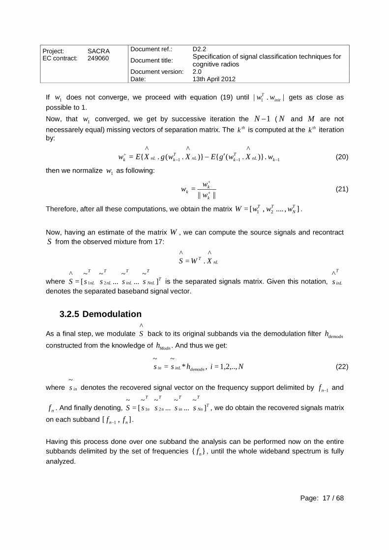
3.2.5 Demodulation
As a final step, we modulate ^S back to its original subbands via the demodulation filter demodnh
constructed from the knowledge of Modnh . And thus we get:
Nihss demodninLin 1,2,..,= ,*~
=~
(22)
where ins~
denotes the recovered signal vector on the frequency support delimited by 1nf and
nf . And finally denoting, T
T
Nn
T
in
T
n
T
n ssssS ]~
...~
...~
~
[=~
21 , we do obtain the recovered signals matrix
on each subband ] , [ 1 nn ff .
Having this process done over one subband the analysis can be performed now on the entire subbands delimited by the set of frequencies }{ nf , until the whole wideband spectrum is fully analyzed.
Project: SACRA EC contract: 249060
Document ref.: D2.2
Document title: Specification of signal classification techniques for cognitive radios
Document version: 2.0 Date: 13th April 2012
Page: 18 / 68
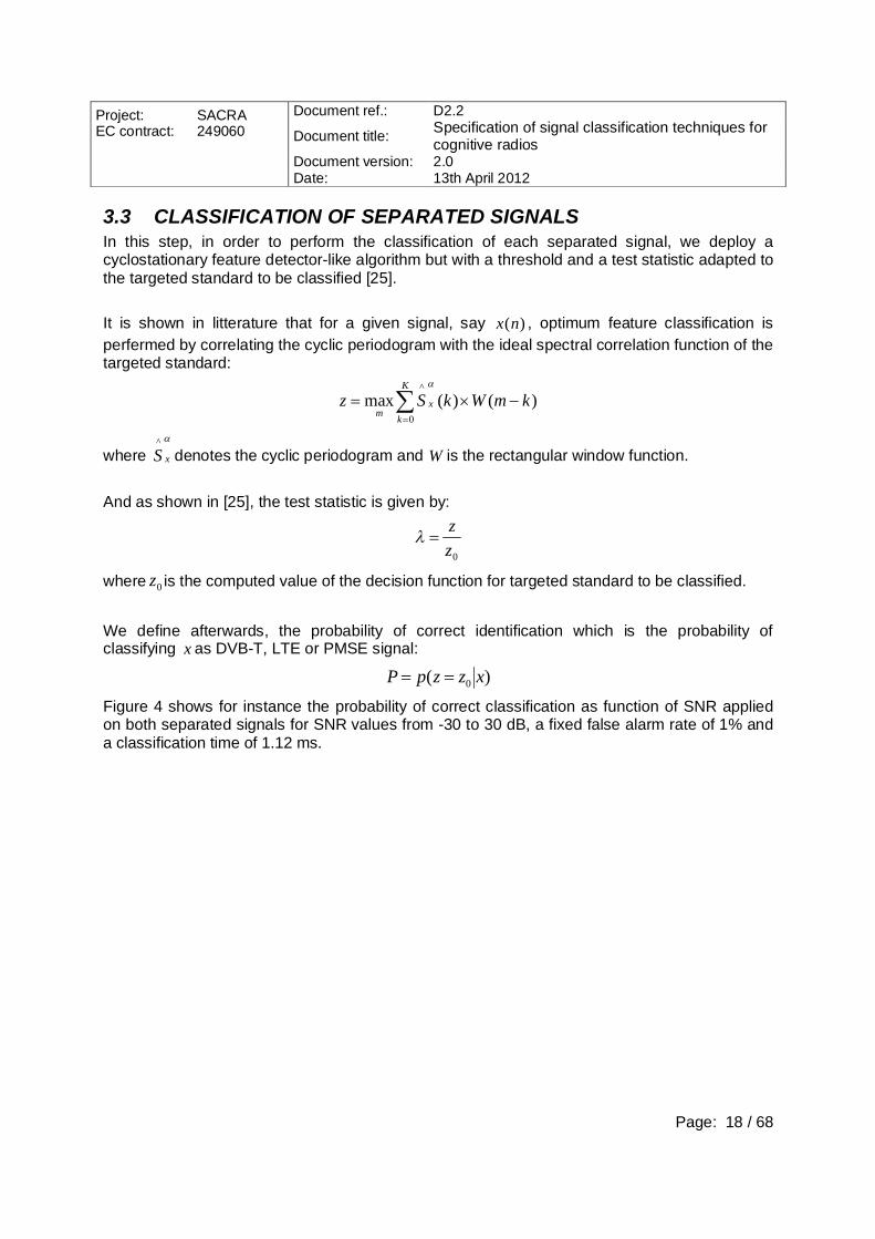
3.3 CLASSIFICATION OF SEPARATED SIGNALS In this step, in order to perform the classification of each separated signal, we deploy a cyclostationary feature detector-like algorithm but with a threshold and a test statistic adapted to the targeted standard to be classified [25]. It is shown in litterature that for a given signal, say )(nx , optimum feature classification is perfermed by correlating the cyclic periodogram with the ideal spectral correlation function of the targeted standard:
)()(max0
^kmWkSz
K
kx
m
where xS^
denotes the cyclic periodogram and W is the rectangular window function. And as shown in [25], the test statistic is given by:
0zz
where 0z is the computed value of the decision function for targeted standard to be classified.
We define afterwards, the probability of correct identification which is the probability of classifying x as DVB-T, LTE or PMSE signal:
)( 0 xzzpP
Figure 4 shows for instance the probability of correct classification as function of SNR applied on both separated signals for SNR values from -30 to 30 dB, a fixed false alarm rate of 1% and a classification time of 1.12 ms.

Project: SACRA EC contract: 249060
Document ref.: D2.2
Document title: Specification of signal classification techniques for cognitive radios
Document version: 2.0 Date: 13th April 2012
Page: 19 / 68
Figure 4: Probability of right classification vs. SNR for DVB-T standard.
-30 -20 -10 0 10 20 300
0.1
0.2
0.3
0.4
0.5
0.6
0.7
0.8
0.9
1
SNR dB
Pro
babi
lity
of ri
ght c
lass
ifica
tion
Classification of DVB-T signals

Project: SACRA EC contract: 249060
Document ref.: D2.2
Document title: Specification of signal classification techniques for cognitive radios
Document version: 2.0 Date: 13th April 2012
Page: 20 / 68
4 LTE SIGNAL CLASSIFICATION WITHOUT QUIET PERIOD LTE, DVB-T and PMSE systems have distinct characteristics that can be used for signal classification. This chapter first describes the LTE signal in Section 4.1, then the primary user signal in Section 4.2. In Section 4.3 we first present the cyclostationary properties of DVB-T, PMSE, and LTE signals, and in Section 4.4 we show the performance of the classification without quiet period, for different scenarios.
4.1 LTE SYSTEM CONSIDERATIONS The LTE system considerations are useful for 2 distinct reasons:
The classification device has to classify PU signals, without erroneously classifying LTE SU instead. For this purpose, one has to know the LTE symbol period and the LTE useful period.
The classification device has to be a User Equipment, which means that the clock frequency and the bandwidth configurations are LTE compliant. As we will further show in the next paragraphs, each system configuration has distinct parameters. The most important ones are the sampling frequency (for a given sensing time, the number of samples impacts the classification) and the system bandwidth (which impacts the total amount of noise captured by the classification device).
4.1.1 LTE Physical Parameters As being specified by 3GPP, the LTE system can be configured to different frequency bands: 1.4 MHz, 3 MHz, 5 MHz, 10 MHz, 15 MHz, 20 MHz. Corresponding to these frequency bands to be used, the IFFT lengths are: 128, 256, 512, 1024, 1536, and 2048 respectively. Similarly, for reasons related to the legacy with UMTS, the sampling frequency is multiple of UMTS chip period: 3.84/2 MHz, 3.84 MHz, 2x3.84 MHz, 4x3.84 MHz, 6x3.84 MHz, and 8x3.84 MHz respectively. It is important to mention that IFFT length is a multiple of 2 for practical implementation issues, but the system itself will not use all the subcarriers. Corresponding to different system configurations, the number of subcarriers being used is: 73, 181, 301, 601, 901 and 1201 respectively, with the middle one called DC subcarrier (and which normally has less energy). As the LTE system bandwidth increases, the total number of the resources increases as well. Therefore, according to the LTE bandwidth being used, the number of resource blocks per symbol is: 6, 30, 50, 100, 150 and 200 respectively. Modulations used by the LTE systems are QPSK, 16-QAM, and 64-QAM. Depending on the channel, LTE system has the following modulation schemes:

Project: SACRA EC contract: 249060
Document ref.: D2.2
Document title: Specification of signal classification techniques for cognitive radios
Document version: 2.0 Date: 13th April 2012
Page: 21 / 68
Physical channel Modulation schemes
PDSCH QPSK, 16QAM, 64QAM
PMCH QPSK, 16QAM, 64QAM
PHICH BPSK
PUCCH BPSK, QPSK, BPSK+QPSK
Table 1: LTE Modulation Schemes
Related to the frame structure, there are 20 slots of 0.5 ms in one frame. It is also important to mention that the OFDM symbol is composed from a useful period and a cyclic prefix (see D2.1 for further explanations). However, different from DVB-T, for LTE systems the useful period is constant (TU=1/(15 KHz)=66,66 µs) but cyclic prefix is not. There are several configurations described below:
Normal CP (7 symbols per slot) o TCP=5.21 µs for the first OFDM symbol from one slot; o TCP=4.69 µs for the last 6 OFDM symbols from one slot.
Extended CP (6 symbols per slot): TCP=16.67 µs. MBSFN only (7.5 kHz subcarrier spacing), the OFDM useful symbol has TU=133.33 µs,
and the cyclic prefix has TCP=33.33 µs – R9 feature (3 symbols per slot)
4.1.2 Cyclic Prefix (CP) in LTE As stated in the previous section, for the normal CP configuration, the CP is not constant. The figure below resumes the impact of having distinct CPs and different sampling rates for different LTE BW configurations.
Figure 5: LTE cyclic prefix and symbol length in number of samples

Project: SACRA EC contract: 249060
Document ref.: D2.2
Document title: Specification of signal classification techniques for cognitive radios
Document version: 2.0 Date: 13th April 2012
Page: 22 / 68
This configuration, of course, will impact the classification properties of LTE systems. Please note that based on this configuration, we have developed an LTE signal generator (for normal and extended CP), and we have used this configuration for different simulations results presented in this chapter.
4.2 PRIMARY USER CONSIDERATIONS This section describes the DVB-T and PMSE (QPSK and FM) signal parameters. The parameters described in this chapter have been further used for classification purposes. However, please note that the classification has to be implemented in the UE LTE device, which means that the PU signals have to be sampled at LTE frequency rate. We have therefore developed primary user signal generators, and we have used these generators for different simulations presented in this chapter.
4.2.1 DVB-T Physical Parameters The guard interval precedes every OFDM symbol and it helps mitigating the inter-symbol interference. Echoes of the previous symbol should abate within the guard interval. Otherwise the echoes would disturb the following OFDM symbol and increase the Bit Error Ratio (BER). Therefore, the required length of the guard interval depends on the application to be covered. An OFDM symbol is composed of two parts: a useful part with duration TU and a guard interval with a duration TCP. The guard interval consists in a cyclic continuation of the useful part, TU, and is inserted before it. A longer guard interval could compensate longer echoes [18]:
lengthening the guard interval without changing the absolute duration of the useful interval would accordingly decrease the channel capacity, thus reducing the deliverable bit rate;
alternatively, lengthening both the guard interval and the useful interval would not bring any penalty to the channel capacity, but would make the signal processing more difficult because of the higher number of carriers that would result from the larger symbol duration.
In summary, the following parameters can be chosen in the DVB-T system:
code rate of inner error protection: 1/2, 2/3, 3/4, 5/6, 7/8.
carrier modulation: QPSK – 2 bit per carrier; 16-QAM – 4 bit; or 64-QAM – 6 bit.
guard interval length: 1/4, 1/8, 1/16, 1/32.
modulation parameter 1 for non-hierarchical; 2 or 4 for hierarchical.
FFT length which can be related to the number of carriers:
o 2k mode with 1 705 carriers,
o 4k mode with 3409 carriers (DVB-T handheld),
o 8k mode with 6 817 carriers. TU/TS: 4/5, 8/9, 16/17 or 32/33 depending on guard interval.
According to [19] the useful symbol period TU of DVB-T is:

Project: SACRA EC contract: 249060
Document ref.: D2.2
Document title: Specification of signal classification techniques for cognitive radios
Document version: 2.0 Date: 13th April 2012
Page: 23 / 68
For 8 MHz DVB-T channel: o 896 µs (8k mode), o 448 µs (4k mode), o 224 µs (2k mode)
For 7 MHz DVB-T channel: o 1024 µs (8k mode), o 512 µs (4k mode), o 256 µs (2k mode)
For 6 MHz DVB-T channel: o 1194,667 µs (8k mode), o 597,333 µs (4k mode) o 298,6667 µs (2k mode)
For 5 MHz DVB-T channel (normative): o 1433,6 µs (8k mode), o 716,8 µs (4k mode), o 358,4 µs (2k mode).
DVB-T Cyclic Prefix can be: 1/4, 1/8, 1/16 or 1/32. In our simulations we have considered 8 MHz DVB-T with useful symbol 224 µs and CP 1/4 (TCP=TU/4).
4.2.2 PMSE Signal Parameters The following documents provide technical information on Radio microphones: ERC Report 42 [20] and ERC Report 88 [21]. During 1991, ETSI was requested to update T/R 20-06 and this work has resulted in three standards [20]:
1. ETS 300 422 Radio Equipment and Systems (RES); Technical characteristics and test methods for radio microphones in the 25 MHz to 3 GHz frequency range
2. ETS 300 454 Radio Equipment and Systems (RES); Wide band audio links; Technical characteristics and test methods
3. ETS 300 445 Radio Equipment and Systems (RES); Electro-Magnetic Compatibility (EMC) standard for radio microphones and similar Radio Frequency (RF) audio link equipment Also, another interesting report useful for the PMSE information regarding the standardization is [9] on PU protection for TVWS. In this report it can be found that PMSE can be analogical or digital, with different frequency bandwidths.
4.2.2.1 Identified PMSE Calibration Procedures PMSE can be analogical (FM) or digital (QPSK) as explained below:
Analogical (FM), with 200 KHz bandwidth o If FM is using a sinusoidal modulated signal: SFM(t)=A*cos(2*pi*f0*t+m*sin(2*pi*f*t)),
where f=25 KHz – the maximum speech frequency

Project: SACRA EC contract: 249060
Document ref.: D2.2
Document title: Specification of signal classification techniques for cognitive radios
Document version: 2.0 Date: 13th April 2012
Page: 24 / 68
o We used Carlson’s equation to generate bandwidth limited FM signals. According to Carlson, 99% of the power is in a frequency band of B=2*f(1+m+sqrt(m)).
o After imposing the frequency band, using f=25 KHz and Carlson’s equation, one obtains the modulation factor m=1.6972.
o It can be shown that -30dB from the peak, the bandwidth of the signal is 200 KHz.
Figure 6: Zoom on FM Signal Spectra, for 6 MHz signal carrier with f=25 KHz.
Numerical (QPSK), with 400 KHz bandwidth
o The symbol period TS is around 2.5 µs, but it differs from this value if Nyquist filters are being used. However, in simulations, for simplification, a rectangular pulse shape filter is usually considered.
o Digital modulations sometimes use Nyquist filters in order to improve signal spectra. In simulations dedicated to PMSE we have also considered roll-off-factors in order to rend the simulation more realistic.
4.2.2.2 PMSE in UK In the UK prior to Digital Switch Over (DSO) CH69 is used exclusively for PMSE, as a result of the Digital Dividend CH69 will be released as part of the upper cleared spectrum (800 MHz spectrum) for mobile broadband applications in the upcoming Ofcom spectrum auction (currently consultations are going on for this). Post DSO, Ofcom has assigned CH38 as the PMSE exclusive channel. Also PMSE can operate in the interleaved spectrum (White spaces) as a licensed secondary service. In the UK before using the channels for PMSE, the channels need to be reserved via JFMG. This is different to other countries in Europe where PMSE operates without prior reservation. More information on PMSE roadmap in the UK can be found in the JFMG website, http://www.jfmg.co.uk/.

Project: SACRA EC contract: 249060
Document ref.: D2.2
Document title: Specification of signal classification techniques for cognitive radios
Document version: 2.0 Date: 13th April 2012
Page: 25 / 68
4.3 CYCLOSTATIONARITY FOR LTE, DVB-T AND PMSE The autocorrelation function ,tRrr
of the received signal tr (in our considered scenarios )()()( tntrtrtr DVBTLTE or )()()( tntrtrtr PMSELTE , with )(tn the white additive
Gaussian noise, )(trLTE the received LTE signal from own secondary system, while )(trDVBT and
)(trPMSE are representing the incumbent PU signals) can be represented by Fourier series expansion as
tjRtR rrrr 2exp,
where is a cyclic frequency, is the entire set of cyclic frequencies, and rrR is the Fourier coefficient, also called Cyclic Autocorrelation Function (CAF). The CAF of the second order autocorrelation function can be written as
2
2
*
2
2
*
2exp)()(1lim
2exp)()(1lim
T
TT
T
TTrr
dttjtrtrT
dttjtrtrT
R
When we refer to CAF we usually refer to the second order CAF described by the previous
equation, but in its time-discrete form as in [14]: 1
0
* )2exp()()(1 rN
nrrr tnjdnrnr
NdR
.
Herein the delay d is normalized by the sampling frequency t, and Nr represents the number of available samples. The Generalized Likelihood Ratio Test (GLRT) algorithm for cyclostationary detection (CD) is computing the covariance matrix
r as in [15]. Based on this covariance matrix, the method
further computes the test statistic Trrrrr rrN )()()( 1 , where
rrrrrr RRr Im,Re)( . The test statistic is then compared with a threshold [16], computed with the help of the following equation:
)2/,1(1arg, ettFAP.
where is the incomplete gamma function. In our simulations we have considered the target false alarm probability used for signal classification 1.0arg, ettFAP .
The table below presents examples of the cyclic frequencies adequate for the most common types of secondary and primary user signals [17]:

Project: SACRA EC contract: 249060
Document ref.: D2.2
Document title: Specification of signal classification techniques for cognitive radios
Document version: 2.0 Date: 13th April 2012
Page: 26 / 68
Type of Signal Cyclic Frequencies (First)
OFDM k/TS, k = ± 0,1,2,… ± TU FM ± 2f0 Does not matter
QPSK k/TS, k = ± 0,1,2,… ± (1/2)TS for k=1
Table 2: Cyclic frequencies for different signal types For an OFDM signal, the peaks in the Cyclic Autocorrelation Function (CAF) are dependent on TU and total symbol duration which is TS=TU+TCP. The CAF will exhibit peaks for =+/-TU and = k/(TU+TCP), k=+/-0,1,2, etc. For a sum of multiple OFDM signals with different parameters (different TU and different TU+TCP), multiple distinct peaks should appear on the cyclic autocorrelation function. Therefore, in general, cyclostationary detection may also be used for signal classification. For normal cyclic prefix (LTE) there are 2 types of guard periods: (1) for the first symbol TCP/TU=10/128; (2) for the rest of the symbols TCP/TU =9/128. The LTE cyclic prefix is very small, thus decreasing the cyclostationary properties. For PMSE QPSK, the bandwidth is BW=400 KHz (or 600 KHz). The symbol period is TS=(1+Roll-Off-Factor)/BW if Nyquist filter is being used. Our cyclostationary tests are considering different roll-off factors. The cyclic frequencies are appearing for multiple of 1/ TS. The cyclic peaks are present for delays =± TS /2 (depending on the configuration); For PMSE FM, the bandwidth BW=200 KHz. The PMSE system has to be carefully calibrated with respect to Carlson formula and required PMSE spectrum mask, meaning that a modulation index m=1.69 has to be used. Cyclic frequencies are present at ±2f0 (residual carrier frequency in the considered band). It is important to mention that FM exhibits cyclostationary peaks for delays ±1/2f when sinusoidal modulated signal is being used. This explains the presence of the secondary lobes (see the graphs from further sections).
4.4 LTE FDD DL SIGNAL CLASSIFICATION WITHOUT QUIET PERIOD
As described in the introductory chapter, the objective of this section is incumbent detection while receiving and decoding data, when LTE system is communicating. As previously presented, Primary Users and Secondary Users have different cyclostationary properties that can be used for signal classification. The considered use case is LTE Frequency-Division Duplexing, in DownLink (DL), which means that the User Equipments (UEs) should have classification capabilities in order to differentiate home system from incumbent system.

Project: SACRA EC contract: 249060
Document ref.: D2.2
Document title: Specification of signal classification techniques for cognitive radios
Document version: 2.0 Date: 13th April 2012
Page: 27 / 68
4.4.1 General Classification Context As presented in the figure below, the general classification context supposes that prior to classification there is sensing: the LTE system first senses that there is no PU in the WS band, and if the PU is not present, the eNodeB will initiate a communication phase (1).
Figure 7: Communication Phase in White Space (WS) frequency band During the communication phase (1), UEs have transmitter (Tx) classification capabilities to differentiate own system from incumbents. As shown later, the classification capabilities allow the SU system to detect when PU is present, while receiving and decoding data in the same time. If a PU starts transmitting, the classification algorithms used by the UEs allow to discriminate between the PU and own SU system. Each UE will therefore inform eNodeB with their classification result. As a result of this measurement, the eNodeB will stop the communication phase in the WS identified as occupied by a PU and will move the communication phase in the licensed band or another WS band which was previously identified as free.

Project: SACRA EC contract: 249060
Document ref.: D2.2
Document title: Specification of signal classification techniques for cognitive radios
Document version: 2.0 Date: 13th April 2012
Page: 28 / 68
Figure 8: Incumbent classification and communication phase in licensed band
4.4.2 General Description of the Algorithm In this section we describe the general classification algorithm. However, as presented in the introductory chapter, SUs coexistence is out of scope of SACRA WP2. As explained in the figure below, the algorithm first checks if the DVB-T PU is being used or not. For this purpose, a cyclostationary detector is being used. If the output is negative, in a second stage the method tries to split the DVB-T frequency band into multibands in order to decrease the total power of the acquired noise.
Figure 9: General description of the classification algorithm

Project: SACRA EC contract: 249060
Document ref.: D2.2
Document title: Specification of signal classification techniques for cognitive radios
Document version: 2.0 Date: 13th April 2012
Page: 29 / 68
Another option is to directly detect the PMSE in the wide frequency band, as presented in the figure below. The advantage of using such a method is to decrease the classification time and the complexity, but as shown in [13] the detection capacity will be slightly lower. The simplified version of the scheme above, when we directly use the LTE system and its sampling rate in order to perform classification is described as follows:
Figure 10: Simplified description of the classification algorithm
The LTE system decides if it stops the WS transmission or not, based on the classification result. Different from the method proposed in Section 3, the method from Section 4 resumes to the following steps:
1. “Is DVB-T?” 2. “Is PMSE?”
Therefore, in this context, it has no point to use signal separation. Another important aspect is that we had to generate waveforms at Rx LTE sampling rate. Therefore, we have generated to mixtures:
DVB-T+LTE+Noise sampled at RX LTE sampling rate (multiple of 3.84 MHz), with possibility to control:
Power of DVB-T (S_DVBT) Power of LTE (S_LTE) Power of Noise (N)
PMSE+LTE+Noise sampled at RX LTE sampling rate (multiple of 3.84 MHz), with possibility to control:
Power of PMSE (S_PMSE) Power of LTE (S_LTE) Power of Noise (N)
The metrics to be used are the probability of DVB-T classification as a function of SNR_DVBT=S_DVBT/N, and probability of PMSE classification as a function of SNR_PMSE=S_PMSE/N.

Project: SACRA EC contract: 249060
Document ref.: D2.2
Document title: Specification of signal classification techniques for cognitive radios
Document version: 2.0 Date: 13th April 2012
Page: 30 / 68
As explained also in the technical annex for sensing algorithms, in order to be able to protect the PU, SACRA system needs a required SNR (required SNR for classification, in our case) smaller than the minimum received SNR (which is imposed by the regulatory body). Based on this statement, and the minimum received SNR imposed by FCC (SNRmin), one can design its algorithms to be in agreement with FCC. We use the equation provided in the technical annex for the conversion between the FCC requirements and SNRmin to compute different thresholds. The classification supposes that the UE classifies while communicating, meaning that the filter used by the UE is the same as the one being employed by the LTE system. In our simulations we have considered a 10 MHz LTE system communicating in TVWS, meaning that the reception filter has 15.36 MHz bandwidth.
4.4.3 DVB-T Signal Classification when LTE System is Transmitting
In Figure 11, we show that CAF DVB-T and CAF LTE characteristics are different. For LTE we have considered a 10 MHz system configuration with normal cyclic prefix, while for DVB-T we have considered an 8 MHz – 2k mode. The figure is showing that DVB-T classification is possible when LTE system is transmitting.
Figure 11: DVB-T and LTE signal classification using CAF
In Table 3, using two different values for the Noise Figure (NF) and the 10 MHz LTE configuration, we have derived two values of SNRmin for DVB-T:
(1) -18.86 dB if the NF = 7 dB and (2) -14.86 dB if the NF = 3 dB.

Project: SACRA EC contract: 249060
Document ref.: D2.2
Document title: Specification of signal classification techniques for cognitive radios
Document version: 2.0 Date: 13th April 2012
Page: 31 / 68
Signal Bandwidth
Pmin Filter Bandwidth
Noise Density (KT)
NF SNRmin
DVB-T 7.6 MHz -114 dBm 8 MHz=69 dBHz (for subband splitting)
-174 dBm/Hz 7 dB -16 dB
DVB-T (1)
7.6 MHz -114 dBm 3.84x4=15.36 MHz=71.86 dBHz
-174 dBm/Hz 7 dB -18.86 dB
DVB-T (2)
7.6 MHz -114 dBm 3.84x4=15.36 MHz=71.86 dBHz
-174dBm/Hz 3 dB -14.86 dB
Table 3: DVB-T SNRmin requirement for classification, under 10 MHz LTE system
configuration Figure 12 shows that 50 ms time is not sufficient for DVB-T classification when LTE is transmitting, if the NF is too high. However, for systems with 3 dB NF, the SNR required might be reached in cases when SNR LTE is sufficiently low (see threshold (2) which was derived for NF=3 dB).
Figure 12: DVB-T classification, when LTE system is communicating, for 50 ms classification time
However, Figure 13 clearly shows that 250 ms classification time is sufficient for DVB-T classification when LTE is transmitting (SNR LTE is 0dB), for both NF=3dB (2) and NF=7dB (1).

Project: SACRA EC contract: 249060
Document ref.: D2.2
Document title: Specification of signal classification techniques for cognitive radios
Document version: 2.0 Date: 13th April 2012
Page: 32 / 68
Figure 13: DVB-T classification, when LTE system is communicating, for 250 ms classification time
4.4.4 PMSE Signal Classification when LTE System is Transmitting Similar to DVB-T signal classification, we show the proof of concept and performance results for PMSE QPSK and PMSE FM respectively.
4.4.4.1 QPSK Signal Classification In Figure 14, Figure 15, and Figure 16 we show that CAF QPSK PMSE and CAF LTE characteristics are different. For LTE we have considered a 10 MHz system configuration with normal cyclic prefix, while for PMSE QPSK we have considered a PMSE Tx with rectangular shaping function (Figure 14), a PMSE Tx with 0.1 roll-off factor (Figure 15) and a PMSE Tx with 0.9 roll-off factor (Figure 16). All graphs are showing that QPSK classification is possible when LTE system is transmitting.

Project: SACRA EC contract: 249060
Document ref.: D2.2
Document title: Specification of signal classification techniques for cognitive radios
Document version: 2.0 Date: 13th April 2012
Page: 33 / 68
Figure 14: PMSE QPSK and LTE signal classification using CAF
Figure 15: PMSE QPSK with 0.1 Roll-Off Factor and LTE signal classification using CAF
Figure 16: PMSE QPSK with 0.9 Roll-Off Factor and LTE signal classification using CAF

Project: SACRA EC contract: 249060
Document ref.: D2.2
Document title: Specification of signal classification techniques for cognitive radios
Document version: 2.0 Date: 13th April 2012
Page: 34 / 68
In Table 4, using FCC’08 and FCC’10 requirements and the 10 MHz LTE configuration, we have derived two values of SNRmin for PMSE QPSK (detected in the LTE wide frequency band):
(1) -15.86dB (NF=7dB) for FCC’08, and (2) 4.14dB (NF=7dB) for FCC’10.
Signal
BW Pmin Filter
Bandwidth Noise Density (KT)
NF SNRmin
PMSE QPSK
400 KHz -111dBm(’08) 8 MHz=69dB -174dBm/Hz 7dB -13dB
PMSE QPSK
400 KHz -111dBm(’08) 400 KHz=56dB (for subband splitting)
-174dBm/Hz 7dB 0dB
PMSE QPSK
400 KHz -104dBm(’10) 8 MHz=69dB -174dBm/Hz 7dB -6dB
PMSE QPSK
400 KHz -104dBm(’10) 400 KHz=56dB (for subband splitting)
-174dBm/Hz 7dB 7dB
PMSE QPSK(1)
400 KHz -111dBm(’08) 3.84x4=15.36 MHz=71.86dBHz
-174dBm/Hz 7dB -15.86dB
PMSE QPSK(2)
400 KHz -104dBm(’10) 3.84x4=15.36 MHz=71.86dBHz
-174dBm/Hz 7dB -8.86dB
Table 4: PMSE QPSK SNRmin requirement for classification, under 10 MHz LTE system configurations
Figure 17 shows the probability of classification in terms of SNR PMSE QPSK, when LTE system is transmitting. A 250 ms classification time (provided by the choice of the DVB-T classification block) is therefore sufficient with respect to both required SNRmin thresholds (FCC’08 and FCC’10).

Project: SACRA EC contract: 249060
Document ref.: D2.2
Document title: Specification of signal classification techniques for cognitive radios
Document version: 2.0 Date: 13th April 2012
Page: 35 / 68
Figure 17: PMSE QPSK classification, when LTE system is communicating, for 250 ms classification time. Similarly to Figure 17, Figure 18 shows the probability of classification in terms of SNR PMSE QPSK, when LTE system is transmitting, for a 0.9 Roll-Off-Factor. A 250 ms classification time (provided by the choice of the DVB-T classification block) is therefore sufficient with respect to both required SNRmin thresholds (FCC’08 and FCC’10) represented in the same figure by (1) and (2).

Project: SACRA EC contract: 249060
Document ref.: D2.2
Document title: Specification of signal classification techniques for cognitive radios
Document version: 2.0 Date: 13th April 2012
Page: 36 / 68
Figure 18: PMSE QPSK (0.9 Roll-Off-Factor) classification, when LTE system is communicating, for 250 ms classification time.
4.4.4.2 FM Signal Classification In Figure 19, Figure 20, and Figure 21 we show that CAF FM PMSE and CAF LTE characteristics are different. For LTE we have considered a 10 MHz system configuration with normal cyclic prefix, while for PMSE FM we have considered a 200 KHz PMSE Tx with 1 MHz frequency carrier (Figure 19), 7 MHz frequency carrier (Figure 20) and 7 MHz frequency carrier represented without adjacent cyclostationary lobes (Figure 21). All graphs are showing that FM classification is possible when LTE system is transmitting.

Project: SACRA EC contract: 249060
Document ref.: D2.2
Document title: Specification of signal classification techniques for cognitive radios
Document version: 2.0 Date: 13th April 2012
Page: 37 / 68
Figure 19: PMSE FM with f=25 KHz, f0=1 MHz (lower part of the captured frequency band) and LTE signal classification using CAF – all the adjacent lobes have been represented
Figure 20: PMSE FM with f=25 KHz, f0=7 MHz (higher part of the captured frequency band) and LTE signal classification using CAF – all the adjacent lobes have been represented
Figure 21: PMSE FM with f=25 KHz, f0=7 MHz (higher part of the captured frequency band) and LTE signal classification using CAF – without adjacent lobes representation
In Table 5, using FCC’08 and FCC’10 requirements and the 10 MHz LTE configuration, we have derived two values of SNRmin for PMSE FM (detected in the LTE wide frequency band):
(1) -18.86dB (NF=7dB) for FCC’08, and

Project: SACRA EC contract: 249060
Document ref.: D2.2
Document title: Specification of signal classification techniques for cognitive radios
Document version: 2.0 Date: 13th April 2012
Page: 38 / 68
(2) -11.86dB (NF=7dB) for FCC’10.
Signal BW
Pmin Filter Bandwidth
Noise Density (KT)
NF SNRmin
PMSE FM
200 KHz -114dBm(’08) 8 MHz=69dB -174dBm/Hz 7dB -16dB
PMSE FM
200 KHz -114dBm(’08) 200 KHz=53dB (for subband splitting)
-174dBm/Hz 7dB 0dB
PMSE FM
200 KHz -107dBm(’10) 8 MHz=69dB -174dBm/Hz 7dB -9dB
PMSE FM
200 KHz -107dBm(’10) 200 KHz=53dB (for subband splitting)
-174dBm/Hz 7dB 7dB
PMSE FM (1)
200 KHz -114dBm(’08) 3.84x4=15.36 MHz=71.86dBHz
-174dBm/Hz 7dB -18.86dB
PMSE FM (2)
200 KHz -107dBm(’10) 3.84x4=15.36 MHz=71.86dBHz
-174dBm/Hz 7dB -11.86dB
Table 5: PMSE FM SNRmin requirement for classification, under 10 MHz LTE system configuration Figure 22 shows the probability of classification in terms of SNR PMSE FM, when LTE system is transmitting. A 250 ms classification time (provided by the choice of the DVB-T classification block) is therefore sufficient with respect to both required SNRmin thresholds (FCC’08 and FCC’10).
Figure 22: PMSE FM classification, when LTE system is communicating, for 250 ms classification time.

Project: SACRA EC contract: 249060
Document ref.: D2.2
Document title: Specification of signal classification techniques for cognitive radios
Document version: 2.0 Date: 13th April 2012
Page: 39 / 68
4.4.5 DVB-T Signal Classification when PMSE and LTE are Transmitting
This section clearly shows that if the DVB-T Tx is not present, the system will not classify DVB-T. According to the figure below, at the left hand side the classification probability equals to the false alarm probability (i.e. 0.1), while at the right hand side the classification probability equals zero.
Figure 23: DVB-T classification when 400 KHz PMSE QPSK, 10 MHz LTE and Noise are present, for 250 ms classification time.
4.5 CONCLUSIONS The objective of this study was to detect while receiving and decoding data (very strong constraint), but in this case the choice of the sensing time will not affect the Quality of Service. The advantage of using classification instead of QP is that the classification time can be (theoretically) as long as possible. Our conclusion is also that the requirements proposed by FCC for sensing can be adapted to classification. Please also note that the classification requirement depends on the following parameters:
o Sensing time; o NF (Noise Figure of the amplification chain from LTE Rx); o LTE configuration – which gives the sampling frequency being used and the detection
BW size; o The amount of DVB-T/PMSE captured in the analyzed BW.
For 10 MHz Bandwidth (Very Wide Band), classification needs at least 250 ms in order to meet the system requirements for DVB-T sensing.

Project: SACRA EC contract: 249060
Document ref.: D2.2
Document title: Specification of signal classification techniques for cognitive radios
Document version: 2.0 Date: 13th April 2012
Page: 40 / 68
5 SIGNAL CLASSIFICATION AND SIGNAL DETECTION EVALUATION
The goal of this chapter is to provide information about SACRA indicators and to describe the indicators that have an impact on D2.2. This section also presents an initial complexity study of sensing and classification algorithms, by comparing the algorithms in terms of number of real multiplications and additions. The last part of the chapter also provides performance comparison results of the two classification algorithms previously described by the Sections 3 and 4.
5.1 SACRA INDICATORS This section resumes the four SACRA indicators described in the technical annex. Please note that the scope of this section is to show how these indicators are related to WP2 and D2.2. The 1st global indicator is the Spectrum Occupancy. As described in the technical annex, “The spectrum occupancy is the average percentage of the used frequency bands in a given frequency band [SH77], [SSC05].” In other words, this parameter defines the percentage of White Spaces before (e.g. 50%) and after (e.g. 99%) the opportunistic access. This is not directly related to detection or to WP2, but it concerns the white space identification and the access technique. Therefore, the spectrum occupancy is a parameter that should be considered by the Radio Resource Manager (RRM), and it does not concern WP2. The 2nd global indicator is the Spectral Efficiency. The spectral efficiency is measured in terms of (bit/s)/Hz usually over the frequency band of a specific system. The theoretical maximum spectral efficiency is defined by the modulation method and by the possible use of spatial multiplexing, which makes it important for WP2.3, and is not the goal of D2.2. The 3rd global indicator is the Energy Efficiency. The energy efficiency indicator is measured in terms in J/bit = W/(bit/s) averaged over a given area where the energy in joules (J) includes both “the transmitted energy and the signal processing energy [GW02]”, and is related to the implementation from WP4. This parameter is represented by the choice of the SACRA RRM, which has to use as much as possible the secondary lower band. This parameter should therefore be considered by RRM, and is not the goal of D2.2. The 4th global indicator is the Number of Components. This is a major objective to reduce the number of components or at least to keep it at the current state of the art level, but with additional functionalities to fulfill previous indicators. This parameter can be related to the number of electronic components, or to the complexity of the algorithms (which can be related to WP2), or to the number of algorithms being used by RRM.

Project: SACRA EC contract: 249060
Document ref.: D2.2
Document title: Specification of signal classification techniques for cognitive radios
Document version: 2.0 Date: 13th April 2012
Page: 41 / 68
The table below resumes all the discussions from the previous paragraphs:
Indicator Impact of the indicator on D2.2
Spectrum occupancy Not the scope of D2.2
Spectral efficiency WP2.3, not the scope of D2.2
Energy efficiency Not the scope of D2.2
Number of components Should be considered in D2.2
Table 6: SACRA indicators and their impact on D2.2.
5.2 ENERGY OPTIMIZATION From the sensing point of view energy optimization depends on the final goal:
o local optimization or o global optimization.
For a given set of requirements (e.g., Detection Probability, False Alarm Probability), energy optimization is done through:
o Local Energy Consumption Minimization Can be done through cooperative sensing – Cooperative sensing is increasing
the global energy consumption, but it can be used to decrease local energy consumption.
Can be done by using less complex sensing algorithms o Global Energy Consumption Minimization
By choosing the lowest energy consuming cooperative sensing algorithm Can be done by using less complex sensing algorithms
5.3 COMPLEXITY STUDY In this section, we will study the complexity of signal separation and signal classification algorithms proposed in Section 3 and Section 4. To compute these complexities, we need information about the complexity of spectrum sensing algorithms described in D2.1 and compared in Section 7 of this deliverable.

Project: SACRA EC contract: 249060
Document ref.: D2.2
Document title: Specification of signal classification techniques for cognitive radios
Document version: 2.0 Date: 13th April 2012
Page: 42 / 68
5.3.1 Spectrum sensing algorithms complexity study Here we will study the complexity of all spectrum sensing algorithms presented in D2.1. We will introduce in this deliverable a spectrum sensing algorithm: pilot correlation based detector (PCD). We will compare this detector to energy detector (ED), Welch detector (WD), cyclostationarity based detector (CD) and algebraic detector (AD). It is well known that the complexity of sensing algorithms is increasing the energy consumption. It can be proved that there is a relationship between the number of samples and the total Computation Load (CL), where the CL is given by total number of instructions (multiplications and additions). Therefore, both the acquisition time and the sampling time have an impact on total CL. The local complexity can be reduced by: o Tuning parameters of a specific sensing algorithm, e.g.:
Welch Method: For a given set of requirements, number of segments used by the periodogram plays an important role in the energy consumption.
Energy Detector : with/without complex noise estimation. Cyclostationary Detector: Data Base assisted/not assisted (the cyclostationary
features are known/not known) o Choosing between different algorithms the one that meets the requirements and has the
smallest complexity.
We assume here that the number of the received samples during the sensing period is N. We also assume that in the case of detection of OFDM signals the period of the cyclic prefix is Tc and the period of the OFDM block is Td. In order to give an idea of the complexity of the studied algorithms we provide a table with the corresponding values for the case of detection of the 8 MHz 2K DVB-T signal (CP=1/4 of useful period and useful signal period is 224 s). Note that these complexity values are approximate. For the simulations, Ls=2048, Nc is the number of samples corresponding to the cyclic period and Nd is the number of samples corresponding to the useful symbol period. We also assume:
• K is the number of cyclic frequencies – in our examples we have considered K=1; • For GLRT, L is the window length used - in our examples we have considered L=101. • M is the number of segments used by Welch Periodogram – in our examples we have
considered M=N/Ls; • Ls is the length of the frequency domain region where signal + noise is estimated – in
our examples we have considered Ls=2048; • Ln is the length of the frequency domain region where noise is being estimated – in our
examples we have considered Ln=Ls/2; • B is the number of sub-bands where noise is being estimated – in our examples we
have considered B=2; • P is the polynomial order for AD – in our examples we have considered P=2.
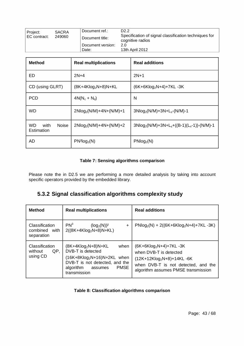
Project: SACRA EC contract: 249060
Document ref.: D2.2
Document title: Specification of signal classification techniques for cognitive radios
Document version: 2.0 Date: 13th April 2012
Page: 43 / 68
Method Real multiplications Real additions
ED 2N+4 2N+1
CD (using GLRT) (8K+4Klog2N+8)N+KL (6K+6Klog2N+4)+7KL -3K
PCD 4N(Nc + Nd) N
WD 2Nlog2(N/M)+4N+(N/M)+1 3Nlog2(N/M)+3N+Ls-(N/M)-1
WD with Noise Estimation
2Nlog2(N/M)+4N+(N/M)+2 3Nlog2(N/M)+3N+Ls+((B-1)(Ln-1))-(N/M)-1
AD PN²log2(N) PNlog2(N)
Table 7: Sensing algorithms comparison
Please note the in D2.5 we are performing a more detailed analysis by taking into account specific operators provided by the embedded library.
5.3.2 Signal classification algorithms complexity study
Method Real multiplications Real additions
Classification combined with separation
PN3 (log2(N))² + 2((8K+4Klog2N+8)N+KL)
PNlog2(N) + 2((6K+6Klog2N+4)+7KL -3K)
Classification without QP, using CD
(8K+4Klog2N+8)N+KL when DVB-T is detected (16K+8Klog2N+16)N+2KL when DVB-T is not detected, and the algorithm assumes PMSE transmission
(6K+6Klog2N+4)+7KL -3K when DVB-T is detected (12K+12Klog2N+8)+14KL -6K when DVB-T is not detected, and the algorithm assumes PMSE transmission
Table 8: Classification algorithms comparison

Project: SACRA EC contract: 249060
Document ref.: D2.2
Document title: Specification of signal classification techniques for cognitive radios
Document version: 2.0 Date: 13th April 2012
Page: 44 / 68
5.3.3 Examples of numerical values for sensing and classification algorithms complexity
The complexity is mainly dependent on both (i) sensing/classification time and (ii) sampling interval (or the sampling period) which is defined by the time period between two samples. As seen in the Tables 7 and 8, both parameters are taken into account by simply using the number of samples N which is defined by the ratio between (i) and (ii). Therefore, in Tables 7 and 8 we have evaluated our algorithms in terms of number of samples N, and other several key parameters which are specific for each algorithm. However, in this section we are providing numerical examples for all previous described algorithms. In Table 9 we have therefore considered that the sensing or classification is performed by a LTE (UE) receiver. If the LTE system is configured to 10 MHz bandwidth, then the sampling period will be 1/(4x3.84 MHz) since the sampling frequency equals 4x3.84 MHz for this given configuration. In Table 9 we have considered a 10 ms sensing/classification time, and the sampling period 1/(4x3.84 MHz), the total number of samples is N=153600.
Method Multiplications Additions Total Number
ED 307204 307201 614405
CD 1.3043e+007 817.3729 1.3044e+007
PCD 2.6419e+009 153600 2.6421e+009
WD 3995649 5529599 9525248
WD with NE 3995650 5530622 9526272
AD 8.1296e+011 5.2927e+006 8.1296e+011
Classif. – Method 1 2.1514e+018 5.2943e+006 2.1514e+018
Classif. – Method 2 (worst case)
2.6086e+007
1.6347e+003
2.6088e+007
Table 9: Sensing algorithms comparison for sensing/classification time = 10ms and sampling frequency 4x3.84 MHz
From the results obtained in the previous table we can easily see that the ED is the less complex sensing algorithm, while the more complex are (in order): WD, WD with Noise estimation, CD, PCD and AD. We have also obtained that the second classification method

Project: SACRA EC contract: 249060
Document ref.: D2.2
Document title: Specification of signal classification techniques for cognitive radios
Document version: 2.0 Date: 13th April 2012
Page: 45 / 68
provided in section 4 is less complex in terms of total number of computations from the method provided in section 3 which uses separation combined with classification.
5.3.4 Conclusion Table 7 presents the comparison in terms of complexity of all studied algorithms. The comparison is performed in terms of multiplications and additions, which are the operations required for the implementation. Some of the algorithms require more complex computations because they include operations such as logarithms or FFTs. From this table, we conclude that the CD, AD and WD detectors are the most complex among all studied algorithms, while PCD and ED detectors are the less complex. Low complexity detectors are desirable since they are cheaper to manufacture and are typically more energy efficient. The latter is important especially if the spectrum sensors are battery operated. Similar to Table 7, Table 8 presents the comparison between the two classification techniques proposed in previous chapters: one technique uses separation combined with classification while the other technique uses only classification. For the first technique the complexity is thus higher since the method is first separating the received signal into two branches and then applies classification on each branch. We have also showed that the complexity of all algorithms is dependent on the number of samples N. Therefore, in Tables 7 and 8 we have evaluated our algorithms in terms of number of samples and other key parameters which are specific for each algorithm. Numerical examples of these evaluations are further provided in Table 9. Please note that in D2.5 we are improving this initial study and we are performing a more detailed analysis by taking into account specific operators provided by the embedded library.
5.4 PERFORMANCE EVALUATION Figure 24 shows the comparison between the two presented techniques above: classification using separation technique and classification without quiet period, for a classification time = 250 ms, a sampling frequency of 4x3.84 MHz and the LTE SNR signal set to 0 dB. From Figure 24, we notice that the direct classification technique over-performs the one proceeded after separation technique as the separation step introduces some distortions and noise to will be added to the simulated noise level as signal to signal plus interference noise.

Project: SACRA EC contract: 249060
Document ref.: D2.2
Document title: Specification of signal classification techniques for cognitive radios
Document version: 2.0 Date: 13th April 2012
Page: 46 / 68
Figure 24: Classification techniques comparison

Project: SACRA EC contract: 249060
Document ref.: D2.2
Document title: Specification of signal classification techniques for cognitive radios
Document version: 2.0 Date: 13th April 2012
Page: 47 / 68
6 CONCLUSIONS In this deliverable, new techniques for the global efficiency of wireless systems were developed in the context of SACRA project. Specifically, we proposed efficient ways of signal separation and signal classification methods for cognitive radio. We’ve been giving a first step towards the final demo by disseminating some preliminary results regarding the specification of signal classification techniques for cognitive radios networks in SACRA context and giving a complete comparison of the sensing algorithms that could be used in terms of performance comparison and complexity. The first proposed algorithm for signals classification in CRN combines signal classification with signal separation. This proposed algorithm for signals classification in CRN contains three steps: a frequency edge location, via algebraic estimation of spectrum edges, and the separation process exploiting blind signal separation techniques followed by a final classification step using DVB-T signals cyclostationarity features. The second part of this document proposes a less complex LTE signal classification technique without Quiet Period, which does not impact the SU QoS. The later method also shows that classification using cyclostationary properties is possible and in agreement with the FCC requirements. A comparison between the two classification techniques in the same simulation framework was provided in order to help choosing which classification technique will be implemented for the final project demonstration.

Project: SACRA EC contract: 249060
Document ref.: D2.2
Document title: Specification of signal classification techniques for cognitive radios
Document version: 2.0 Date: 13th April 2012
Page: 48 / 68
7 APPENDIX: SPECTRUM SENSING ALGORITHMS EVALUATION
We will present in this appendix the simulation setup and report the performance simulation results related to sensing techniques proposed by the consortium and presented in D2.1. We will compare these techniques in terms of detection capability using SACRA constraints and their computational complexity. The final objective of this comparison is to choose and implement a proper spectrum sensing scheme in an existing cognitive radio scenario on the EURECOM OpenAirInterface platform. An evaluation framework will be introduced in this appendix to compare spectrum sensing algorithms proposed in D2.1. Please note that the state of art presented in the first section of this chapter, section related to sensing requirements, it is also used for classification purposes in the current deliverable.
7.1 SENSING REQUIREMENT This section is divided in two main parts: a part describing primary user protection requirements and another part describing the conversion between primary user protection requirements and Signal to Noise Ratio SNR (which is used by SACRA in order to evaluate the performance of different algorithms).
7.1.1 Primary User Protection Requirements This section presents the sensing requirements as extracted from FCC, CEPT, 802.22 and OFCOM technical reports.
7.1.1.1 FCC 2008 (nov.) From the point of view of FCC, the detection threshold is similar to the sensing threshold, which is the minimum received power from the PU that has to be sensed, i.e. Pmin. According to FCC [5], all fixed and personal/portable TVBDs must be capable of detecting ATSC digital TV, NTSC analogue TV and wireless microphone signals using analogue or digital modulation methods. The required detection thresholds are:
ATSC signals: -114 dBm, averaged over a 6 MHz bandwidth; NTSC signals: -114 dBm, averaged over a 100 KHz bandwidth; Wireless microphone signals: -114 dBm, averaged over a 200 KHz bandwidth.
In the same report it is mentioned that for the DVB-T Detection, some parties suggested a minimum sensing threshold of -114 dBm per 6 MHz bandwidth. This is equivalent to -132dBm in a 100 KHz bandwidth.

Project: SACRA EC contract: 249060
Document ref.: D2.2
Document title: Specification of signal classification techniques for cognitive radios
Document version: 2.0 Date: 13th April 2012
Page: 49 / 68
On the other hand, for PMSE Detection, according to I2R and Philips the sensing devices used during their tests were able to detect wireless microphones at levels ranging from -103 dBm to -129 dBm depending on the type of microphone. Apparently they have also noticed some detection issues when DVB-T is used in adjacent channels.
7.1.1.2 FCC 2010 (sept.) According to this new report published by FCC in September 2010 [6], the required detection thresholds are:
ATSC digital TV signals: -114 dBm, averaged over a 6 MHz bandwidth; NTSC analog TV signals: -114 dBm, averaged over a 100 KHz bandwidtI(C) Low power
auxiliary, including wireless microphone, signals: -107 dBm, averaged over a 200 KHz bandwidth.
This FCC report seems more complete, as it also defines other parameters such as:
(1) Channel availability check time. A TVBD may start operating on a TV channel if no TV, wireless microphone or other low power auxiliary device signals above the detection threshold are detected within a minimum time interval of 30 seconds. (2) In-service monitoring. A TVBD must perform in-service monitoring of an operating channel at least once every 60 seconds. There is no minimum channel availability check time for in-service monitoring. (3) Channel move time. After a TV, wireless microphone or other low power auxiliary device signal is detected on a TVBD operating channel, all transmissions by the TVBD must cease within two seconds.
In the same report it can be found that SBE, Shure and CWMU argue that the sensing level should be lowered to -126 dBm as is required in the United Kingdom.
7.1.1.3 FCC 2010 (nov.) The previous FCC report [6] was more favourable to the database dynamic spectrum access approach. As a result of this, in November 2010 FCC published an addendum [7] to the previous report from September. This report clearly shows that spectrum sensing is “an important component of dynamic spectrum use” and that “sensing permits a dynamic spectrum access radio to detect unused spectrum by autonomously determining current use of a particular frequency”. In the same report one can also find that spectrum sensing techniques can be classified into three categories
transmitter detection, cooperative detection, interference-based detection.

Project: SACRA EC contract: 249060
Document ref.: D2.2
Document title: Specification of signal classification techniques for cognitive radios
Document version: 2.0 Date: 13th April 2012
Page: 50 / 68
Transmitter detection provides these radios the capability of determining if a signal from a primary user’s transmitter is locally present by correlating a known signal with an unknown signal (matched filter detection), measuring signal energy (signal detection), or statistical means (cyclostationary feature detection or some other pattern recognition method). In is important to notice that this technical report shares the same view as SACRA, regarding the sensing methods and categories being used in technical literature. This report also defines some other terms such as “cooperative detection” and “interference-based detection”. Cooperative detection therefore refers to incorporating information from multiple dynamic users to determine if spectrum is in use by a primary user. Similarly, interference-based detection refers to detecting changes in the local noise floor to determine if additional traffic can be tolerated by primary users.
7.1.1.4 CEPT Different from FCC, in CEPT [9] one can also find a technical term called “receiver sensitivity”. Receiver sensitivity generally refers to the sensitivity of the PU Rx, as it is defined by the following statement: “The reference sensitivity level of a receiver is the minimum wanted signal power for which the receiver can operate correctly in a noise-limited environment.” Receiver sensitivity can therefore be defined as a threshold under which decoding is no longer possible. CEPT presents White Space Device (WSD) detection threshold computation which was derived from PU Rx sensitivity. The detection threshold therefore depends on the white space device characteristics, deployment scenarios, and BS/receiver configurations. At last, detection threshold seems to have the same meaning as the sensing threshold and the definition provided by FCC. This CEPT report [9] mentions a sensing time of 5ms, and cites 802.22. One can easily identify 3 paragraphs of particular interest for the study conducted in this chapter:
(1) A wireless microphone user would normally expect the microphone to be usable within about 2 seconds after it is switched on. (2) The sensing duration before a WSD decides that a channel is available. This is usually a large number, for example 30 secs in the FCC rules. This ensures that temporal fades do not cause an erroneous decision. (3) The in-service sensing duration which is typically much smaller, for example 5 ms every 160 ms as specified in the IEEE 802.22 standard.
From the first and the last paragraphs we could deduce that, for the IEEE 802.22 standard, 12 detections are possible during 2 seconds (as the periodicity of sensing is 160 ms). However, this means a total detection time of 5x12=60 ms (as the sensing time is about 5ms). From the second paragraph we could easily see that initial detection can be longer, as it is recommended by FCC.

Project: SACRA EC contract: 249060
Document ref.: D2.2
Document title: Specification of signal classification techniques for cognitive radios
Document version: 2.0 Date: 13th April 2012
Page: 51 / 68
It is also important to mention that for PMSE, sensing threshold has been defined for 6 scenarios, and each of them have 6 detection threshold derivations: - Scenario 1 - WSD is located far enough from the PMSE: detection threshold is -119dBm. - Scenario 2 - Hand-held wireless microphones: detection threshold is -121 to -156 dBm. - Scenario 3 - Body pack wireless microphones: detection threshold is -132 to -167 dBm. - Scenario 4 - In-ear monitor: detection threshold is -80 to -115 dBm. - Scenario 5 - Studio (10 mW handheld wireless microphone and 100 mW handheld WSD
with 100m path length between the WSD and elevated (10m) PMSE RX (Di) and 200m low path length between the WSD and PMSE TX (Dd)): -120 to -155 dBm.
- Scenario 6 - Sport event (10 mW handheld wireless microphone and 100 mW handheld WSD with 36m path length between the WSD and elevated (20m) PMSE RX (Di) and 1300m low path length between the WSD and PMSE TX (Dd)): -120 to -155 dBm.
7.1.1.5 802.22 After a very detailed review of 802.22 standard [8], we have found that even if it is cited by CEPT (see previous section), 5ms is not explicitly presented as sensing duration in 802.22 standard. However, 10 ms is the frame duration and 160 ms is the superframe duration. Two sensing times are mentioned:
1. The intra-frame sensing stage - which is comprised of one sensing period per frame, during which sensing algorithms that requires quiet periods of less than one frame size are employed; 2. The inter-frame sensing stage - which supports sensing algorithms that require longer sensing durations. The inter-frame sensing stage is longer than one frame size.
7.1.1.6 OFCOM Concerning OFCOM decision regarding PU detection threshold, it seems that OFCOM proposes a -126 dBm detection threshold requirement. This detection threshold has been defined as the PMSE min power required for detection and it was computed for a 200 KHz PMSE channel. OFCOM also describes a higher required detection probability than previous mentioned reports. This required detection probability is 99.99%. However, same as the FCC report, channel move time is considered less than 2 seconds.
7.1.2 Conversion between the Regulatory Sensing Requirements and SNR
This section describes the conversion between the previously presented standardization requirements and SNR. This conversion it is important in order to evaluate the performance of our algorithms in terms of SNR.

Project: SACRA EC contract: 249060
Document ref.: D2.2
Document title: Specification of signal classification techniques for cognitive radios
Document version: 2.0 Date: 13th April 2012
Page: 52 / 68
7.1.2.1 Receiving Scheme The figure below describes the conversion from Pmin to SNR. Please note that minimum received power which has to be sensed is a parameter used by FCC, CEPT and OFCOM. However, as in 802.22, in SACRA we use Signal to Noise Ratio, as it incorporates the captured noise power in the bandwidth B, by the Rx band-pass filter.
Figure 25: Receiving scheme
The total received noise power is considered to be the product of the noise density KT and the bandwidth B:
KTBBandwidthtyNoiseDensiNoisePower where K is the Boltzman constant, T is the temperature and B is the bandwidth of the pass-band filter. Based on this definition of the noise power one can define SNRmin as the ratio between the minimum received power at the end of transmission chain and the received noise power, which would be linearly expressed as:
NoisePowerNFPSNR /min
min ,
and when expressing it in [dB], the same equation becomes
][log10]/[][][][ 10minmin HzdBBHzdBmKTdBNFdBmPdBSNR . In our algorithms, we denote by the SNRreq the SNR required to reach a detection probability of 90% (other alternatives would be PD=95% or PD=99% for example). Obviously, according to regulatory bodies, this means that the necessary condition for a good detection would be
reqSNRSNRmin
The previous discussion can be therefore resumed to the following phrase: In order to be able to protect the PU, SACRA system needs a required SNR (required SNR for sensing

Project: SACRA EC contract: 249060
Document ref.: D2.2
Document title: Specification of signal classification techniques for cognitive radios
Document version: 2.0 Date: 13th April 2012
Page: 53 / 68
and/or classification algorithms) smaller than the minimum received SNR (which is imposed by the regulatory body). Based on these results, in the next sections the reader may find tables with the conversion between the requirements imposed by different regulatory bodies, for different primary signals, and the minimum SNR to be sensed.
7.1.2.2 Requirements conversion for DVB-T Signal Signal
Bandwidth Pmin Filter
Bandwidth Noise Density (KT)
NF SNRmin
DVB-T 7.6 MHz -114dBm 8 MHz=69dB -174dBm/Hz 7dB -16dB
Table 10: The minimum SNR level for DVB-T – conversion from FCC
7.1.2.3 Requirements conversion for PMSE 200 KHz
Signal Signal Bandwidth
Pmin Filter Bandwidth
Noise Density (KT)
NF SNRmin
PMSE (1) 200 KHz -119dBm 8 MHz=69dB -174dBm/Hz 7dB -21dB
PMSE (1) 200 KHz -119dBm 200 KHz=53dB -174dBm/Hz 7dB -5dB
PMSE (2) 200 KHz -156dBm 8 MHz=69dB -174dBm/Hz 7dB -58dB
PMSE (2) 200 KHz -156dBm 200 KHz=53dB -174dBm/Hz 7dB -42dB
PMSE (3) 200 KHz -167dBm 8 MHz=69dB -174dBm/Hz 7dB -69dB
PMSE (3) 200 KHz -167dBm 200 KHz=53dB -174dBm/Hz 7dB -53dB
PMSE (4) 200 KHz -115dBm 8 MHz=69dB -174dBm/Hz 7dB -17dB
PMSE (4) 200 KHz -115dBm 200 KHz=53dB -174dBm/Hz 7dB -1dB
PMSE (5) 200 KHz -155dBm 8 MHz=69dB -174dBm/Hz 7dB - 57dB

Project: SACRA EC contract: 249060
Document ref.: D2.2
Document title: Specification of signal classification techniques for cognitive radios
Document version: 2.0 Date: 13th April 2012
Page: 54 / 68
PMSE (5) 200 KHz -155dBm 200 KHz=53dB -174dBm/Hz 7dB -41dB
PMSE (6) 200 KHz -155dBm 8 MHz=69dB -174dBm/Hz 7dB -57dB
PMSE (6) 200 KHz -155dBm 200 KHz=53dB -174dBm/Hz 7dB -41dB
Table 11: The minimum SNR level – CEPT
Signal Signal
Bandwidth Pmin Filter
Bandwidth Noise Density (KT)
NF SNRmin
PMSE 200 KHz -114dBm(‘08) 8 MHz=69dB -174dBm/Hz 7dB -16dB
PMSE 200 KHz -114dBm(‘08) 200 KHz=53dB -174dBm/Hz 7dB 0dB
PMSE 200 KHz -107dBm(‘10) 8 MHz=69dB -174dBm/Hz 7dB -9dB
PMSE 200 KHz -107dBm(‘10) 200 KHz=53dB -174dBm/Hz 7dB 7dB
Table 12: The minimum SNR level – FCC 2008 and 2010
Signal Signal Bandwidth
Pmin Filter Bandwidth
Noise Density (KT)
NF SNRmin
PMSE 200 KHz -126dBm 8 MHz=69dB -174dBm/Hz 7dB -28dB
PMSE 200 KHz -126dBm 200 KHz=53dB -174dBm/Hz 7dB -12dB
Table 13: OFCOM (based on Pmin averaged for 200 KHz)
7.1.2.4 Requirements conversion for PMSE 400 KHz (extrapolated from 200 KHz)
Signal Signal
Bandwidth Pmin Filter
Bandwidth Noise Density (KT)
NF SNRmin
PMSE 400 KHz -111dBm(‘08) 8 MHz=69dB -174dBm/Hz 7dB -13dB

Project: SACRA EC contract: 249060
Document ref.: D2.2
Document title: Specification of signal classification techniques for cognitive radios
Document version: 2.0 Date: 13th April 2012
Page: 55 / 68
PMSE 400 KHz -111dBm(‘08) 400 KHz=56dB -174dBm/Hz 7dB 0dB
PMSE 400 KHz -104dBm(‘10) 8 MHz=69dB -174dBm/Hz 7dB -6dB
PMSE 400 KHz -104dBm(‘10) 400 KHz=56dB -174dBm/Hz 7dB 7dB
Table 14: The minimum SNR level – FCC 2008 and 2010 (based on Pmin averaged for 400 KHz)
Conclusion: After the conversion, FCC seems more reasonable in terms of sensing requirements as the SNRmin imposed by the FCC seems less difficult to attend compared with CEPT (for several scenarios) or Ofcom for example.
7.2 REVIEW OF SPECTRUM SENSING ALGORITHMS Spectrum sensing algorithms proposed by SACRA project partners are described in D2.1 deliverable. In this appendix, we will compare these algorithms and we will give recommendations about suitable sensing algorithms for different spectrum sensing tasks. The sensing algorithms presented in D2.1 can be classified into three categories based on the amount of information used for the sensing purpose:
7.2.1 Energy detection These detection algorithms do not make any assumption on PU signal characteristics. Basically these techniques are detecting random signal in noise. They do not need much prior information on the signal but on the other hand, these methods are not able to exploit the detailed information we typically have of primary signal waveforms. However, very accurate information on noise statistics is necessary in order to obtain reliable performance. We presented in D2.1 two sensing algorithms based on energy detection: the classical energy detector (ED) that measures the received energy during a finite time interval and compares it to a predetermined threshold. The second detector is the algebraic detector (AD), proposed also in D2.1
7.2.2 Welch periodogram The same as ED, Welch periodogram is also based on the detection of the received signal energy. It attempts to improve the statistical properties of the periodograms by dividing the received data sequence into segments and performing averaging over the segments. Using Welch periodogram, the signal energy can be measured in the band(s) of interest simultaneously. In addition, it enables to estimate the energy of the noise from the regions where the signal is less predominant. More details on the Welch periodogram can be found in D2.1 and [10].

Project: SACRA EC contract: 249060
Document ref.: D2.2
Document title: Specification of signal classification techniques for cognitive radios
Document version: 2.0 Date: 13th April 2012
Page: 56 / 68
7.2.3 Feature detection Feature detection algorithms employ knowledge of structural and statistical properties of PU signals in the decision making. Such properties include cyclostationarity, autocorrelation property and finite alphabet property, for example. The cyclostationarity based detector (CD) was described in D2.1 and was implemented for comparison with other detectors.
7.2.4 Matched filter detection These algorithms assume explicit knowledge of a pilot waveform or preamble, i.e. they are detecting known signals in noise and interference. For example, detector based on DVB-T pilots. However these detectors are suitable to detect only one particular PU signal and cannot be used to detect other PU signals. We will describe in the following the DBT-T pilot correlation based detector (PCD) which was not described in D2.1 deliverable. In order to estimate the channel conditions, some predefined pseudo-noise sequences are integrated in the transmitted signal. These are known as “pilot” sequences. Alternatively, in multicarrier transmissions such as DVB-T some subcarriers may be dedicated for transmitting pilot signals [1]. Pilot signals may be scattered over the subcarriers and over the time depending on the coherence time and coherence bandwidth of typical channel. The PU standards are usually known and these sequences are defined correspondingly. Based on the knowledge of these sequences various detection algorithms can be defined.
Let us assume that the transmitted signal {xk}k= 0N
consists of a known “pilot” part {mk}k=0N
and
unknown “information” part {wk}k=0N
, i.e.
x k =wk +mk , k=0,1,2 , .. . ,N .
Since the sequence {mk}k=0N
is known we can define a test statistics in the following way
.+k
N
=kkCP my=
The parameter is used in this case for synchronization to the received signal in time domain. Usually the pilot sequences are periodical with some period M. Thus the search for should be over one period. The test statistics CP should have a clear “peak” value when we have synchronization between the received sequence and the pilot sequence. Thus we can define
max= CP1M0,1,2,...,CP ,
as it has been done in [1]. Taking the maximum real part, i.e.
max= CP1M0,1,2,...,CP ,
is also possible choice that outperforms the previous one in many cases [1].

Project: SACRA EC contract: 249060
Document ref.: D2.2
Document title: Specification of signal classification techniques for cognitive radios
Document version: 2.0 Date: 13th April 2012
Page: 57 / 68
7.3 EVALUATION FRAMEWORK 7.3.1 Performance evaluation criteria
In D2.1, several spectrum sensing schemes have been proposed for SACRA project. Each scheme may have a different performance in a different scenario. It is therefore important to compare and choose the best scheme for a given scenario. For a fair comparison, it is necessary to choose proper performance criteria. In this section, we present important performance evaluation parameters:
1. False alarm probability Pfa: False alarm probability is defined as the probability that the detector declares the presence of PU, when the PU is actually absent. Controlling the false alarm probability is crucial in order to make sure that the cognitive radio system is not overwhelmed with alarms and to ensure that some data will get transmitted.
2. Miss detection probability Pmd: This is defined as the probability that the detector declares the absence of PU, when the PU is actually present. It is a crucial parameter as a high value of Pmd may result in increase in the interference to PU and consequently retransmissions and reduced rate and quality of service. Note that probability of detection Pd and miss detection probability are related to each other Pd = 1 - Pmd. Therefore for simulation results, without loss of any generality, we have used Pd.
3. SNR regime: This is range of SNRs over which detector should perform sensing reliably. SNR regime depends on desired sensor coverage. Spectrum sensing schemes should detect PU signal reliably in low SNR regime as the PU receivers which are far away from the transmitter should not be interfered with. However it is also important that the sensor does not detect PU signals with too low SNR values, i.e., PUs which are well outside its cover age.
4. Sensing time: It is important that vacant frequency bands are quickly detected so that
they can be used efficiently. If sensing time is too long, the data transmission duration reduces, thereby reducing throughput of SUs.
5. Complexity and implementation issues: Algorithms can also be compared from the
implementation point of view by estimating the hardware cost and energy efficiency through computational complexity of the algorithm.
There are trade-offs among the desired performance parameters. Therefore, the most common way to compare different sensing scheme is to plot:
1. Probability of detection curve as a function of SNR for a given false alarm probability and sensing time.
2. Receiver operating curve (ROC), i.e., probability of detection as a function of false alarm probability for a given SNR and sensing time.
Complexity study was treated in Section 5.3.1.

Project: SACRA EC contract: 249060
Document ref.: D2.2
Document title: Specification of signal classification techniques for cognitive radios
Document version: 2.0 Date: 13th April 2012
Page: 58 / 68
7.3.2 Evaluation scenario In our evaluation framework we have concentrated on the single sensor detection techniques. The primary system used is a DVB-T system. DVB-T abbreviates Digital Television Broa–cast - Terrestrial, and as the name implies it is a standard for wireless digital transmission of TV signals. The standard is administered by the European Telecommunications Standards Institute (ETSI). The official ETSI web page can be found at [3]. In DVB-T, there are two modes in 8 MHz channel, 2K and 8K modes, which set the number of carriers in the OFDM symbol. In 2K and 8K modes there are actually 1,705 or 6,817 subcarriers and subcarriers are approximately 4 or 1 KHz apart, respectively. Three different modulation schemes (QPSK, 16QAM, 64QAM) can be used. As a digital transmission, DVB-T delivers data at the symbol rate in a series of discrete blocks. In DVB-T, a COFDM (coded OFDM) transmission technique including variable length guard interval is used. The choice of the DVB-T system is justified by the fact that many of the current and especially future wireless systems utilize the OFDM modulation format. In addition, one target in SACRA project is to study secondary use, i.e. spectrum sensing, of the spectrum in the UHF band, extended to TVWS (TV white space) where DVB-T is utilized in the frequency range above 470 MHz. The simulation scenarios are generated by using different combinations of parameters given in Table 1.The channel models implemented are AWGN, Rician and Rayleigh channels. The latter two correspond to the two different types of propagation that have to be handled in practice, namely line-of-sight (LOS) and non-line-of-sight (NLOS). Slow fading is simulated by adding log-normal shadowing. Bandwidth 8MHz Mode 2K Modulation 16QAM Guard interval 1/4 Channel models AWGN/Rayleigh/Rician (K=10) Maximum Doppler shift 100Hz Frequency-flat Single path Sensing time 1.12ms Location variability 10dB
Table 15: The transmitted DVB-T primary user signal parameters Three different scenarios with different properties have been chosen to evaluate the spectral detection performance, subject to provide different attributes so that the performance can be assessed under different conditions, aiming to provide fair conditions before making conclusions. OFDM is the modulation of choice for the three simulation scenarios to be used as evaluation tools in this report. In OFDM, a wideband channel is divided into a set of narrowband orthogonal subchannels. OFDM modulation is implemented through digital signal processing via to the FFT algorithm [4].
1. Scenario 1 uses a DVB-T OFDM signal in an AWGN channel. It is assumed that the detection performance in AWGN will provide a good impression of the performance, but it is necessary to extend the simulations to include signal distortion due to multipath and shadow fading.

Project: SACRA EC contract: 249060
Document ref.: D2.2
Document title: Specification of signal classification techniques for cognitive radios
Document version: 2.0 Date: 13th April 2012
Page: 59 / 68
2. Scenario 2 utilizes the same DVB-T OFDM signal as scenario 1, but to make the simulations more realistic, the signal is subjected to Rayleigh multipath fading and shadowing following a log normal distribution in addition to the AWGN. The maximum Doppler shift of the channel is 100Hz and the standard deviation for the log normal shadowing is 10dB. Since the fading causes the channel to be time variant, it is necessary to apply longer averaging than in scenario 1 to obtain good simulation results. Thus the number of iterations in the Monte Carlo simulation is increased from 500 to 1000.
3. Scenario 3 utilizes also a DVB-T OFDM signal in Rician multipath fading with shadowing. The K-factor for the Rician fading is 10, which represents a very strong line of sight component. The maximum Doppler shift of the channel and the standard deviation for the log normal shadowing are the same as in the second scenario.
7.4 SIMULATION RESULTS AND DISCUSSION The evaluation framework has been implemented in Matlab and all results are obtained as the average of a number of Monte Carlo simulations. For the Monte Carlo simulation, each signal block consists of one symbol which contains 2048 samples. 500 iterations are performed in the simulation. We will give in the following simulation results using the three scenarios described in Section 7.3.2.
7.4.1 Probability of detection vs SNR curves
Figure 26: Performance evaluation of the sensing detectors using a DVB-T OFDM system in AWGN channel ( = 0.05 and sensing time = 1.12 ms)

Project: SACRA EC contract: 249060
Document ref.: D2.2
Document title: Specification of signal classification techniques for cognitive radios
Document version: 2.0 Date: 13th April 2012
Page: 60 / 68
Figure 27: Performance evaluation of the sensing detectors using a DVB-T OFDM system in Rayleigh multipath fading and shadowing channel ( = 0.05 and sensing time = 1.12 ms)
Figure 28: Performance evaluation of the sensing detectors using a DVB-T OFDM system in Rician multipath fading and shadowing channel ( = 0.05 and sensing time = 1.12 ms)

Project: SACRA EC contract: 249060
Document ref.: D2.2
Document title: Specification of signal classification techniques for cognitive radios
Document version: 2.0 Date: 13th April 2012
Page: 61 / 68
Figure 29: Performance evaluation of the sensing detectors using a DVB-T OFDM system in AWGN channel ( = 0.05 and sensing time = 10 ms)
Figure 30: Performance evaluation of the sensing detectors using a DVB-T OFDM system in Rayleigh channel ( = 0.05 and sensing time = 10 ms)
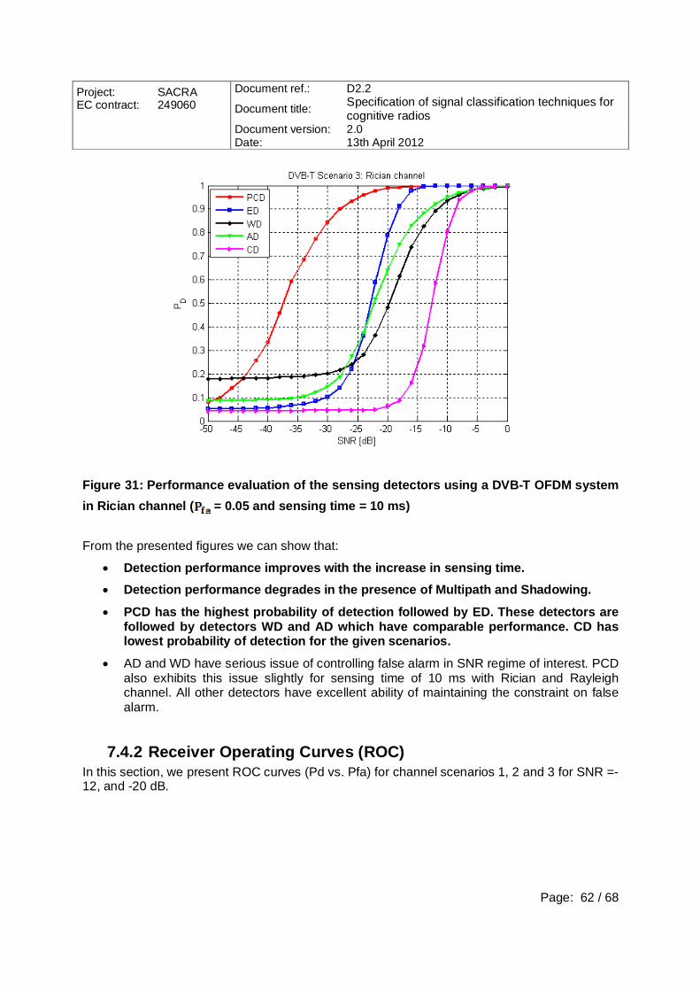
Project: SACRA EC contract: 249060
Document ref.: D2.2
Document title: Specification of signal classification techniques for cognitive radios
Document version: 2.0 Date: 13th April 2012
Page: 62 / 68
Figure 31: Performance evaluation of the sensing detectors using a DVB-T OFDM system in Rician channel ( = 0.05 and sensing time = 10 ms) From the presented figures we can show that:
Detection performance improves with the increase in sensing time. Detection performance degrades in the presence of Multipath and Shadowing.
PCD has the highest probability of detection followed by ED. These detectors are followed by detectors WD and AD which have comparable performance. CD has lowest probability of detection for the given scenarios.
AD and WD have serious issue of controlling false alarm in SNR regime of interest. PCD also exhibits this issue slightly for sensing time of 10 ms with Rician and Rayleigh channel. All other detectors have excellent ability of maintaining the constraint on false alarm.
7.4.2 Receiver Operating Curves (ROC) In this section, we present ROC curves (Pd vs. Pfa) for channel scenarios 1, 2 and 3 for SNR =-12, and -20 dB.

Project: SACRA EC contract: 249060
Document ref.: D2.2
Document title: Specification of signal classification techniques for cognitive radios
Document version: 2.0 Date: 13th April 2012
Page: 63 / 68
Figure 32: Performance evaluation of the sensing detectors using a DVB-T OFDM system in AWGN channel (SNR = -20 dB sensing time = 1.12ms)
Figure 33: Performance evaluation of the sensing detectors using a DVB-T OFDM system in Rayleigh channel (SNR = -12 dB sensing time = 1.12 ms)

Project: SACRA EC contract: 249060
Document ref.: D2.2
Document title: Specification of signal classification techniques for cognitive radios
Document version: 2.0 Date: 13th April 2012
Page: 64 / 68
Figure 34: Performance evaluation of the sensing detectors using a DVB-T OFDM system in Rician channel (SNR = -12 dB sensing time = 1.12 ms)
Figure 35: Performance evaluation of the sensing detectors using a DVB-T OFDM system in Rayleigh channel (SNR = -20 dB sensing time = 1.12 ms)

Project: SACRA EC contract: 249060
Document ref.: D2.2
Document title: Specification of signal classification techniques for cognitive radios
Document version: 2.0 Date: 13th April 2012
Page: 65 / 68
Figure 36: Performance evaluation of the sensing detectors using a DVB-T OFDM system in Rician channel (SNR = -20 dB sensing time = 1.12 ms) From these results, it can be observed that all detectors perform quite well for SNR=-12dB and sensing time of 1.12 ms for AWGN scenario (these results are not presented in this document, we obtain = 1 for all detectors). However, the performance deteriorates with decrease in SNR for detectors ED, WD, AD and CD. Comparative performance of the detectors is similar to Pd vs. SNR curves.
7.5 CONCLUSION In this appendix, we presented simulation results related to spectrum sensing techniques. For this, five sensing techniques are implemented and integrated in a common frameworks using DVB-T primary system. Simulations using different scenarios with different properties were presented in order to compare sensing techniques in term of detection performances. The objective of this comparison is to choose a proper sensing scheme in an existing cognitive radio scenario on the EURECOM OpenAirInterface platform. We selected PCD to sense DVB-T signals and ED to sense PMSE signal.

Project: SACRA EC contract: 249060
Document ref.: D2.2
Document title: Specification of signal classification techniques for cognitive radios
Document version: 2.0 Date: 13th April 2012
Page: 66 / 68
8 ACRONYMS AWGN Additive White Gaussian Noise
AD Algebraic Detector
BSS Blind Signal Separation
CD Cyclostationarity based Detector
CR Cognitive Radio
CRN Cognitive Radio Network
DL DownLink
DSO Digital Switch Over
DVB-T Digital Video Broadcasting-Terrestrial
ED Energy Detector
ETSI European Telecommunications Standards Institute
FC Fusion Center
FCC Federal Communications Commission
FTP File Transfer Protocol
GLRT Generalized Likelihood Ratio Test
QoS Quality of Service
QP Quiet Period
LOS Line-Of-Sight
LTE Long Term Evolution
NLOS Non-Line-Of-Sight
PCD Pilot Correlation based Detector
PMSE Programme Making and Special Events
PU Primary User
ROC Receiver Operating Characteristics
SU Secondary User
TV TeleVision
TVWS TeleVision White Spaces
UEs User Equipments
UL UpLink
WD Welch Detector
WSD White Space Device

Project: SACRA EC contract: 249060
Document ref.: D2.2
Document title: Specification of signal classification techniques for cognitive radios
Document version: 2.0 Date: 13th April 2012
Page: 67 / 68
9 REFERENCES [1] D. Danev, "On signal detection techniques for the DVB-T standard", in Proceedings of the
4th International Symposium on Communications, Control and Signal Processing, March 2010.
[2] L. Lv, Z. Wu, M. Jie, S.-Y. Chang, J. Zhang, J. Wang, S. Li, Q. Peng, L. Chen, and M. Zeng, "Sensing scheme for DVB-T," IEEE 802.22-05/0263r0, Tech. Rep., Nov. 2006.
[3] Official Web Page. European telecommunications standards institute. http ://www.etsi.org. [4] A. Goldsmith. Wireless Communications. Cambridge Univ. Press, New York, 2005. [5] Federal Communications Commission, Technical Report FCC 08-260, Nov. 2008. [6] Federal Communications Commission, “Second memorandum opinion and order”, Technical
Report FCC 10-174, Sept. 2010, Available online: http://www.fcc.gov/ [7] Federal Communications Commission, Technical Report FCC 10-198, Nov. 2010 [8] P802.22/D2.08, May 2009, http://www.ieee802.org/22/ [9] ECC CEPT, “Technical and Operational Requirements for the Possible Operation of
Cognitive Radio Systems in the ”White Spaces” of the Frequency Band 470-790 Mhz,” CEPT, Tech. Rep. 159, Jan 2011.
[10] A. Hekkala, I. Harjula, D. Panaitopol, T. Rautio, and R. Pacalet, ”Cooperative spectrum sensing study using Welch periodogram,” 11th International Conference on Telecommunications (ConTEL 2011). Graz, Austria, 15-17 June 2011, pp. 67-74.
[11] Z. Tian and G. B Giannakis. “A wavelet approach to wideband spectrum sensing for cognitive radios. In Cognitive Radio Oriented Wireless Networks and Communications, 2006. 1st International Conference on, page 1.5, 2006.
[12] D. K. Lin, M. W. Ho, “Exploiting multiple antennas for spectrum sensing in cognitive radio networks”, Patent US 2010266002 (A1).
[13] N. Milosevic, D. Panaitopol, A. Bagayoko.,“Wide-Band Cooperative Spectrum Sensing Method”, CogART 2011.
[14] D. Panaitopol, R. Datta and G. Fettweis, “Cyclostationary Detection of Cognitive Radio Systems using GFDM Modulation”, IEEE WCNC 2012.
[15] A. Dandawate and G. B. Giannakis, “Statistical tests for presence of cyclostationarity,” in IEEE Trans. Signal Process., 1994.
[16] D. Birru, K. Challapali, and B. Dong, “Detection of the presence of television signals embedded in noise using cyclostationary toolbox,” in US Patent 2010/0157066, 2010.
[17] D. Panaitopol, A. Bagayoko, P. Delahaye, and L. Rakotoharison, “Fast and Reliable Sensing Using a Background Process for Noise Estimation,” in In Proc. CrownCom, 2011.
[18] ETSI TR 101 190 V1.3.1, “Digital Video Broadcasting (DVB); Implementation guidelines for DVB terrestrial services; Transmission aspects”
[19] EN 300 744, “Framing structure, channel coding and modulation for digital terrestrial television”.
[20] CEPT ERC REPORT 42, “Handbook on Radio Equipment and Systems Radio Microphones and Simple Wide Band Audio Links”
[21] CEPT ERC REPORT 88, “COMPATIBILITY AND SHARING ANALYSIS BETWEEN DVB–T AND RADIO MICROPHONES IN BANDS IV AND V”.

Project: SACRA EC contract: 249060
Document ref.: D2.2
Document title: Specification of signal classification techniques for cognitive radios
Document version: 2.0 Date: 13th April 2012
Page: 68 / 68
[22] JFMG website: http://www.jfmg.co.uk/ [23] D. Liu, C. Li, J. Liu, K. Long, “A Novel Signal Separation Algorithm for Wideband
Spectrum Sensing in Cognitive Networks”, GLOBECOM 2010, 2010 IEEE Global Telecommunications Conference, 6-10 Dec. 2010, Miami, FL, USA.
[24] W. Guibène, M. Turki, B. Zayen, A. Hayar, “Spectrum Sensing for Cognitive Radio Exploiting Spectrum Discontinuities Detection”, EURASIP Journal on Wireless Communications and Networking (to appear soon)
[25] P.D. Sutton, K.E. Nolan, L.E. Doyle, “Cyclostationary Signatures in Practical Cognitive Radio Applications”, Selected Areas in Communications, IEEE Journal on, page(s): 13 – 24, Jan. 2008.
[26] K.K. Shyu, M.H. Lee, Y.T. Wu, P-L Lee, « Implementation of Pipelined FastICA on FPGA for Real-Time Blind Source Separation », Neural Networks, IEEE Transactions on, June 2008 pages: 958 – 970.