SABP-A-005

Previous Issue: None Next Planned Update: 1 January 2009 Page 1 of 54 Primary Contact: [email protected], phone +966 (3) 873-6045

Best Practice

SABP-A-005 28 December 2005 Quick Energy Assessment Methodology for Energy Efficiency Optimization Document Responsibility: Energy Systems Unit/ESD/CSD

Quick Energy Assessment Methodology for Energy Efficiency Optimization

Document Responsibility: Energy Systems Unit/ESD/CSD SABP-A-005 Issue date: 28 December 2005 Quick Energy Assessment Methodology Next Update: 1 January 2009 for Energy Efficiency Optimization

Page 2 of 54

Table of Contents Page

1.0 Introduction 3

1.1 Definition 3

1.2 Purpose and Scope 3

1.3 Intended Users 4

1.4 Initial Assessment Objectives 4

2.0 Quick Energy Assessment Overview 4

2.1 Energy Efficiency Optimization Task Description 4

2.2 Solution Method Using Decomposition Approach 5

3.0 Methodology 3

3.1 Energy Flow Diagrams 7

3.2 Steam and Power Diagram 11

3.3 Fuel Diagram 12

3.4 Energy Saving Housekeeping List 13

3.5 Energy Saving Generic Checklist 14

4A.0 Appendices for Short-cut Calculations and HGP Energy Study 16

4A.1 Basic Steam Mass Balance 16

4A.2 Basic Energy Utility Targeting Using Pinch Method 18

4A.3 Basic Formulas for Some Quick Savings Estimation 52

4A.4 HGP Detailed Energy Assessment Study 54


Page 3 of 54

1.0 Introduction Energy conservation in Saudi Aramco became everyone’s business. It is mandatory for each process facility to find cost effective solutions to save energy and achieve more with less in their facilities. Saudi Aramco has constituted a committee called EMSC Energy Management Steering Committee to direct and manage a sustainable process for energy conservation. A vital contribution towards the success of the company wide energy conservation policy comes through documenting the company best practices in methodology, tools and applications in the field of energy conservation and distributing such knowledge among our facilities. Hence, a consistent effort has been exerted in Saudi Aramco to produce Best Practices to help Saudi Aramco plants achieve their energy conservation targets and disseminate energy conservation knowledge. This particular Best Practice document for initial energy assessment is a contribution towards this goal. It is expected to draw the line in conducting energy assessments through a user-friendly methodology. The theme of this quick energy assessment methodology for energy efficiency optimization is, “Big Picture First, Details Later”. Energy assessments, also called energy audits, may be primitive or comprehensive and detailed. A variety of approaches, methods and tools are available to conduct such “energy assessments” to improve the energy efficiency of industrial processes.

1.1 Definition The term “Energy Assessment” refers to the methodology of collecting and analyzing available energy utilities related data in order to establish the “big picture” of the breakdown of energy consumption for a particular facility and identify component-based-energy saving opportunities within the facility.

1.2 Purpose and Scope The purpose of this best practice document is to describe a methodology and introduce short cut tools by which quick assessment for energy efficiency improvement can be conducted faster, cheaper and better. Its scope include quick energy assessment methodology in a step-by-step manner, simple models for data representation, checklists for identifying areas for energy savings and short cut tools for creating and evaluating process initiatives for energy saving for common use in Saudi Aramco plants.


Page 4 of 54

1.3 Intended Users

This Best Practice manual is intended for use by the energy engineers working in Saudi Aramco plants, who are responsible for efficient operation of their facility. This particular document will enable them to conduct quick energy assessments systematically.

1.4 Initial Assessment Objectives • Preliminary review of plant process, system drawings and Data gathering

• Understand the “Big Picture” of the plant-wide operations

• Understand process energy and utility systems

• From the available data, establish your current reality

• Establish your desired result “Targeting”

• Identify All Opportunities for energy savings

• Propose Quick-hit savings

• Propose scope for definitive assessment with some economic analysis

• Propose plant-wide energy-utility strategy or “Total energy Management”

2.0 Quick Energy Assessment Overview The first priority in any plant initial energy assessment effort is to define the “quick hits” for energy cost savings that can be achieved with little or no investment. The best practice document does not only help plants energy groups conduct a quick energy assessment for both short and long term energy savings opportunities but also establish the procedures and checklists that can enable process engineers and operators make intelligent choices on hour-to-hour basis.

2.1 Energy Efficiency Optimization Task Description Energy Efficiency Optimization Task aims to specify the near-optimal operation targets/modes that minimize the plant’s energy consumption at minimum deficiency in energy supply of the utility systems to the plant’s process. Following that, the task will be to list all possible operational and design modifications necessary to achieve the specified/desired target(s). This includes identification of all related engineering activities in a minimum possible time using uncertain plant data and without any interruption to the plant’s normal production. This task shall achieve the following two objectives:


Page 5 of 54

1. Minimum disruption in the energy utility supply

2. Minimum consumption of energy utility. “Given an industrial facility that consists of several processes and utility plants, define; at minimum deficiency in energy utility systems supply to the process; near-optimal targets for energy consumption minimization, find a list of possible operational and design modifications to achieve desired target(s) and conduct the engineered solutions”

2.2 Solution Method Using Decomposition Approach For simplicity and timely results, Decomposition Techniques will be used in lieu of the time-consuming Mathematical Programming/Optimization Techniques. The plant’s energy utility needs will be defined with reasonable level of flexibility and the energy utility system; electricity, fuel, steam and other energy-related utilities will be scrutinized one by one to find the near- optimal consumption of such utilities that guarantee minimum deficiency in the utility supply to plant processes. On the macro level the energy system components are generation, distribution and utilization. The objective will be to minimize waste in energy fresh resources and capital (de-bottlenecking) in these three components. This can be done via the continuous upgrade of the efficiency of energy system components in generation, distribution and utilization. However, the utilization component has a unique feature, where its boundaries are not completely dictated by the process. Therefore the room of improvement in this component is much wider than the others.

3.0 Methodology There are four essential tasks that can be conducted by a small energy focus group of three engineers: 1. Data, Models and Targets

2. Insights, Opportunities and Estimated savings potential

3. Screen and Formulate Strategy

4. Document, Report and Present

These tasks are exhibited in the 10-Steps procedures below. 1. Site survey through templates, checklists and interviewing of process

owners/proponents to gather the right amount of data that enable the energy team build the plant’s “big picture” and understand the goals and the constraints of the facility( What to look for and what to ask)


Page 6 of 54

2. Define the criteria for focusing on potential areas of interest (when to be rigorous and get to the second level of details)

3. Develop site energy/utility nominal design/normal operation models with the appropriate level of details in a high level generic “path” diagrams for, power, fuel, H2, steam, water, nitrogen and air. Preliminary purpose of these models will be to understand what is going on in the energy utility system, locate the “energy consumption elephants” (ECEs) in both process and utility plants and generate insights for energy saving opportunities

4. Add more depth in the level of details of the energy utility model for each ECE and/or other criterion of focus

5. Define the effect of disturbances and uncertainty on the energy utility system models

a. Sources of disturbances

b. Site energy utility balance under disturbances

c. Nominal and dynamic targeting of energy utility systems

d. (Check that the “big picture” depicted for the process and the utility plants is correct with enough degree of confidence before you proceed)

6. Target (order of magnitude targeting)

a. _ Identify main processing issues that affect utility utilization

b. _ Link utility-utility interactions

c. _ Integrate and qualitatively optimize site utilities (If we do not coordinate between steam and fuel systems we may stop flaring steam but flaring fuel) for energy utility saving

7. Integrate core processes among themselves and with utilities

8. Develop a comprehensive initiatives list via identifying and estimating energy utility savings opportunities

a. Housekeeping list

b. Checklists (generic and process specific)

c. Waste energy recovery (pinch method and others)

d. In-process Modification (pinch method and others)

9. Champion a cross-fertilizing discussion among plant disciplines to prioritize, screen the initiatives and writing a project sheet, for each initiative, including a description of the opportunity and energy utility savings estimate

10. Develop “word” strategies for realizing savings from facility goals, analysis of the results and the mapping of the opportunities onto the facility strategy (remember, 50% of something is better than 100% of nothing). Then report and present results.


Page 7 of 54

3.1 Energy Flow Diagrams

3.1.1 Overview

Energy Generation

Energy Distribution

Energy Utilization

FuelEnergy Sources

SteamElectricity

Buildings & Others Process

Boilers & Cogeneration

EnergyByproducts

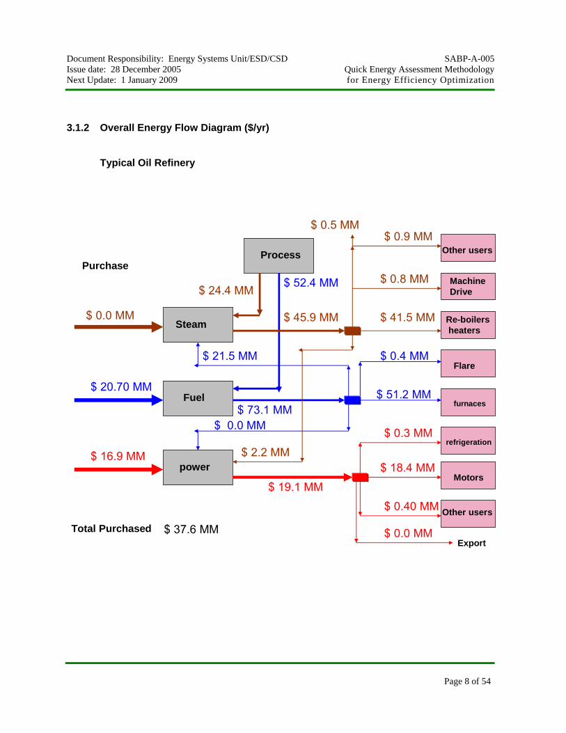
The task now is to look for the “Elephants” in the energy-process system. The graphs below will enable the Energy Engineer to find the “Elephants” to focus his/her efforts and decide where to start and insist on accurate data collection to further proceed with the analysis. Money-based graphs will help quickly to pinpoint the areas of focus. Furthermore, the BTU-based graphs will double check the pre-defined priority list, direct the study towards the process reasons behind certain energy “elephant” and find more efficient ways to satisfy the process target(s).


Page 8 of 54

3.1.2 Overall Energy Flow Diagram ($/yr)

Typical Oil Refinery

Total Purchased

Fuel

Steam

power

ProcessPurchase

Motors

refrigeration

Other users

Export

furnaces

Flare

Re-boilers heaters

MachineDrive

Other users

$ 0.0 MM

$ 20.70 MM

$ 19.1 MM

$ 37.6 MM

$ 21.5 MM

$ 52.4 MM$ 24.4 MM

$ 73.1 MM$ 0.0 MM

$ 51.2 MM

$ 0.4 MM

$ 16.9 MM$ 18.4 MM

$ 0.3 MM

$ 0.40 MM

$ 0.0 MM

$ 45.9 MM

$ 0.5 MM

$ 0.8 MM

$ 41.5 MM

$ 0.9 MM

$ 2.2 MM


Page 9 of 54

Typical Gas Plant

Total Purchased

Fuel

Steam

power

SA Fuel GasPurchase

$ 0.0 MM/yr

$ 0.0 MM/yr

$ 56.1 MM/yr

$ 56.1 MM/yr“200 MW”

$ 19.618 MM/yr

$ 20.018 MM/yr“ 2.54 MM Ib/hr”

$ 0.0 MM/yr

$ 20.018MM/yr

$ 0.0 MM/yr

$ 0.4 MM/yr

$ 56.1 MM/yr

$18.08 MM/yr

$3.25 MM/yr

$29.04 MM/yr

$19.618 MM/yr $0.11MM/yr

$ 0.0 MM/yr

Sulfur RecoveryArea

Utility Area

Gas Comp.Area

Liquid RecoveryArea

Gas TreatArea

Inlet Area

Flare Area

Export

$1.72MM/yr

$0.335MM/yr

$0.609MM/yr

$0.221MM/yr

$2.8 MM/yr

$0.27 MM/yr

$16.6MM/yr

$0.244MM/yr

Note: These Data are Shedgum’sGas Plant


Page 10 of 54

3.1.3 Overall Energy Flow Diagram (Trillion-Btu/yr)

Electricity Fuel steam

Total Input= 10.56 TBtu2 TBtu

8.38 TBtu0.18 TBtu

Boilerssteamcogen

Boilerssteamcogen

Boilerssteamcogen

ProcessProcessBuilding Building Building

BoilerFuel

ConventionalElectricity

-0.19 TBtu 5.77 TBtu - 5.4 TBtu

-0.19 TBtu

BoilerFuel


0.0 TBtu -5.4 TBtu 0.0 TBtu

BoilerFuel


5.59 TBtu 0.18 TBtu

Process

1.8 TBtu0.39 TBtu 0.5 TBtu 2.11 TBtu 0.12 TBtu5.46 TBtu

Area #1 Area #1 Area #1# N # N # N

# NUnit #1# NUnit #1# NUnit #1

Heating Cooling/Ref Machine Drive Electro-Chem Other use7.56 TBtu 0.55 TBtu 1.24 TBtu 0.0 TBtu 0.02 TBtu


Page 11 of 54

3.2 Steam and Power Diagram

Steam “big picture” shall exhibit at least steam sources, pressure levels, mass balance, let down valves and turbines, main users and losses such as vents, let downs and condensate. These information can be used as depicted in the way below to generate ideas and opportunities for saving under the main theme of “Big picture first, and details later.”

chemicals

Proc. #1

Proc. #1

Proc. #1

Proc. #2

Proc. #3

Proc. #4

BFWRaw water Make-up Treatment Plant

MP Process Condensate

LP Process Condensate

HP Process Condensate

Process CondensateEst. 50 % Returned

HP Boiler

MP Boiler

HP

MP

LP

Vent

Effluent

Deaerator

98 t/h

68 t/h

4 t/h

21 t/h 0.0 t/h

68 t/h

30 t/h

0.0 t/h

8 t/h

30 t/h

0.0 t/h

Vent

1 t/h

2 t/h

1 t/h

18 t/h

7 t/h 4 t/h

27 t/h 13 t/h

40 t/h

49 t/h

103 t/h

5 t/h

0.0 t/h0.0 t/h

0.0 t/h

6.28 MW

2 t/h

Steam TargetsEnhance the recovery ofSteam from condensate

Reduce letdown via turbineflow increase or new turbine

Heat integration of process#1 and # 4Estimated saving of 10%

Enhance condensate recoveryBy 10 %

Shut down MP boiler

Eliminate vent

Consider replacing turbines with motors

Reduce and make use of boiler blow-down

Reduce it via operating atlower pressure


Page 12 of 54

3.3 Fuel Diagram

Fuel “big picture” shall exhibit at least fuel sources, pressure levels, mass balance, let down valves and compressors and main users. Hydrogen composition should also be considered to define the opportunities for recycles.

Hydrogen Off-Gas Fuel Gas

5 psig

15 psig

50 psig

52 psig

150 psig150 psig

180 psig

350 psig

400 psig

380 psig

PSA

NG

boilers furnaces


Page 13 of 54

3.4 Energy Saving “Housekeeping” list

1. Establish steam trap auditing program to determine the number of traps (working,

leaking, blocking…etc.) and periodically check it and repair or replace the defected ones

2. Condensate recovery (maintenance and operation)

3. Piping insulation (maintenance)

4. Shutting off equipment when not required (load management)

5. Minimize slow rolling of steam turbines

6. Boilers and furnaces tuning through better combustion control

7. Preventive maintenance of energy system components such as heat exchangers, pumps, fans, compressors, turbines, furnaces, boilers (e.g., clean the fin fan tubes of gas coolers)

8. Improved cooling water system (maintenance and operation)

9. Optimize air compressors operation

10. Optimize BFW pumps load allocation

11. Energy monitoring and indices/ energy management system

12. Shut down compressors at low feed rate (load management)

13. Steam trap management (consider self regulating electrical tracing)

14. Booster, shipper and condensate pumps load management

15. Compressors load management

16. Consider the use of Economizers and Pre-heater in the boilers

17. Compressed air leaks (maintenance)

18. Minimize boilers and water coolers blow downs

19. Utilize boiler blow-down

20. Turbines load management

21. Upgrade sluggish response control valves since the delay might result in extra flaring

22. Enhance the efficiency of boilers and furnaces through tight control

23. Enhance boilers and furnaces insulation

24. Optimize the CHP system


Page 14 of 54

25. Maintain plant steam reserve

26. Minimize/Eliminate the use of steam reducing stations and vents

27. Consider the reuse of turbo-expander to generate power in the HP/LP pressure control valves

28. Enhance the combustion process in boilers and furnaces via using full additives as a catalyst

3.5 Energy Saving “Generic” Checklist

1. Replace gas turbines with more efficient steam turbines

2. Increase boiler steam pressure and temperature to the extent that matches process needs unless electricity generation is the controlling factor

3. Use auxiliary turbines to minimize steam let downs

4. Use steam in the process instead of venting it

5. Preheat combustion air

6. Use ASD on BFW pumps

7. Reduce process variability using stable ops program

8. Trim/Optimize the fired heaters excess oxygen

9. Optimize the fired heaters stack temperature

10. Re-use the flue gases in process heating

11. Optimize your waste heat boilers

12. Recover valuable gases from your fuel gases

13. Reduce the H2 wheel in your plant

14. Cool down the inlet temperature to compressors

15. Reduce cooling medium return temperature in refrigeration cycles

16. Upgrade, regenerate and replace your catalyst

17. Optimize let down stations and steam turbine operation

18. Use highest efficiency turbines

19. Maintain your steam turbines to reduce steam consumption

20. Give frequent attention to steam traps and leaks

21. Replace turbine drives with electric motors if more economical since they are more efficient


Page 15 of 54

22. Boilers and furnaces efficiency enhancement through advanced process control, on-line performance monitoring and optimization

23. Recover condensate

24. Thermal Heat and power integration (CHP)

25. Better control for dispersion steam to flare stacks

26. Optimize steam use in strippers

27. Minimize live steam utilization

28. Mechanical energy integration

29. Reduce natural gas consumption by understanding fuel gas sinks and constraints

30. Reduce fuel gas use with energy integration

31. Keep H2 separate from fuel gas system

32. Measure the composition of off-gas streams and recover C2 and C3+

33. Avoid unnecessary processing of off-gas

34. Avoid unnecessary processing of wastes and inert

35. Minimize the unnecessary production of off-gas

36. Use on-line monitoring and APC for furnaces and other control sensitive fuel users

37. Avoid unnecessary recycles

38. Avoid leaks in the pressure relieve valves to the fuel system

39. Adjust operating pressures and optimize process interaction

40. Clean and maintain pipelines and valves to minimize pressure drops

41. Clean and maintain Boiler tubes from deposits & scale for better operations

42. Treat and recycle blow down to force lower cycles of concentration in cooling towers and boilers

43. Use lowest quality water

44. Maximize use of stripped sour water

45. Minimize generation of wastewater

46. Seek out and repair all hydrocarbon leaks

47. Eliminate direct water injection for cooling purposes

48. Eliminate live steam used for re-boiling and stripping where it is only used for BTU value

49. Minimize or eliminate live steam consumption in sour water strippers by replacing it with re-boilers


Page 16 of 54

50. Boiler blow-down could be considered for cooling tower make-up

51. Extract the low pressure steam from the boiler blowdown

52. Consider re-using the boiler blowdown for reserving the boiler

53. Use process water effluent as a source on the next lower water quality level

54. Eliminate live steam usage since it becomes water and follows an energy path through the plant consuming more energy to process it

55. Should live steam becomes necessary optimize the amount used through pressure manipulation

56. Use lowest quality water possible for desalter operation

57. Minimize water used in desalter

58. Automate desalter operation, avoid water slipping through with crude during desalting/maximize the separation of free water upstream of the crude desalting (each Ib of water will require roughly Ib steam for processing)

59. Minimize the water-wheel in the plant

60. Maximize utilization of treated oily-water from the waste-water treatment plant

61. Install low NOX burners

62. Consider the use of Cogeneration

63. Adjustable speed motors/devices for pumps, compressors, etc.

64. Increase waste heat steam generation

65. Insulate condensate return lines, valves, flanges, etc.

66. Cooling- tower blow-down should not be treated but segregated to sewer

67. Boiler blow-down should not be sent to wastewater treatment but segregate to sewer.

Revision Summary 28 December 2005 New Saudi Aramco Best Practice.


Page 17 of 54

4A.0 Appendices for Short-Cut Calculations and HGP Energy Study

4A.1 Basic Steam Mass Balance The basic Steam Mass Balance does not require high accuracy as long as the developed model still makes sound engineering sense. (i.e., output is much higher than input). Common engineering sense shall be used to estimate what the unknowns. For example condensate return, blow-down and flares can be defined after getting good idea about main consumers.

chemicals

Proc. #1

Proc. #1

Proc. #1

Proc. #2

Proc. #3

Proc. #4





Process CondensateEst. 50 % Returned

HP Boiler

MP Boiler

HP

MP

LP

Vent

Effluent

Deaerator

98 t/h

68 t/h

0.0 t/h

21 t/h 0.0 t/h

68 t/h

30 t/h

0.0 t/h

8 t/h

30 t/h

0.0 t/h

Vent

1 t/h

2 t/h

1 t/h

18 t/h

7 t/h 4 t/h

27 t/h 9 t/h

38 t/h

(42+5) t/h

98+5 t/h

5 t/h

0.0 t/h0.0 t/h

0.0 t/h

6.28 MW


Page 18 of 54

4A.2 Basic Energy Utility Targeting Using Pinch Method

The purpose of this section is not to conduct a pinch study but to get some energy targets regarding the utilities consumption for a desired plant area. This can be done essentially via three methods, graphical, algebraic and using mathematical programming/optimization. In this document the first two methods are going to be explained. Graphical Method: Background: Any heat exchanger can be represented as a hot stream that is cooled down by another cold stream and/or cold utility and a cold stream that is heated up by a hot stream and/or hot utility with a specified minimum temperature approach between the hot and the cold called ∆Tmin. The process exhibited below in the graph shows the situation when the two streams do not have a chance of overlap that produce heat integration between the hot and the cold.


Page 19 of 54

PROCESSH CFeed Product

0

20

40

60

80

100

120

0 10 20 30 40 50 60 H

T HOT UTILITY

COLD UTILITY


Page 20 of 54

Moving the cold stream to the left on the enthalpy axis without changing its supply and target temperatures till we have small vertical distance between the hot stream and the cold stream we obtain some overlap between the two streams that result in heat integration between the hot and the cold and less hot and cold utilities. As been depicted in the graph below with shrinkage in the hot and cold lines span.


0

20

40

60

80

100

120

0 10 20 30 40 50 60 H

T HOT UTILITY

COLD UTILITY

HEAT RECOVERY

Pinch(MAT)


0

20

40

60

80

100

120

0 10 20 30 40 50 60 H

T HOT UTILITY

COLD UTILITY

HEAT RECOVERY

Pinch(MAT)

For demonstration, all hot streams will be represented in the process by one long hot stream to be called “the hot composite curve”. Same thing be done for all cold streams in the process.


Page 21 of 54

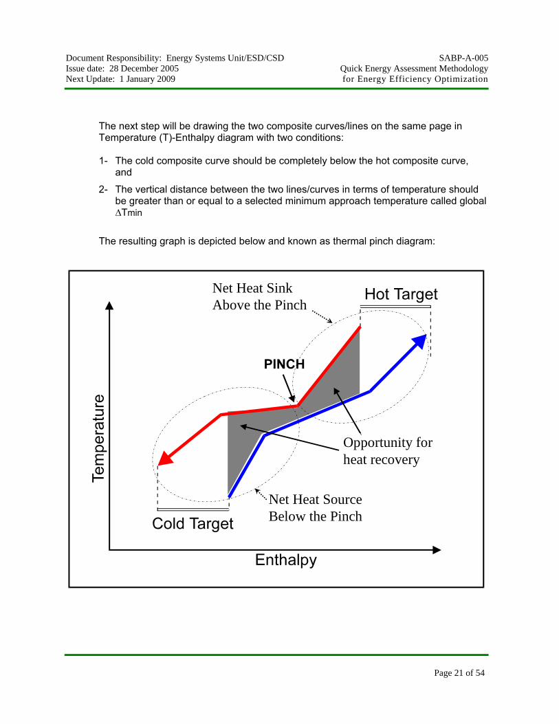
The next step will be drawing the two composite curves/lines on the same page in Temperature (T)-Enthalpy diagram with two conditions: 1- The cold composite curve should be completely below the hot composite curve,

and

2- The vertical distance between the two lines/curves in terms of temperature should be greater than or equal to a selected minimum approach temperature called global ∆Tmin

The resulting graph is depicted below and known as thermal pinch diagram:

Net Heat SinkAbove the Pinch

Net Heat SourceBelow the Pinch

Opportunity for heat recovery

Net Heat SinkAbove the Pinch

Net Heat SourceBelow the Pinch

Opportunity for heat recovery


Page 22 of 54

1. Constructing the composite curves (step-by-step) The above mentioned process can proceed as follows: Stream Type Supply Temperature (ºC) Target Temperature (ºC) FCp (kW/ ºC) 1-Hot 170 70 10 2-Hot 120 30 20 3-Cold 50 90 40 4-Cold 20 110 18 1- Draw the hot composite curve and the cold composite curve via developing the

following tables. Note: The tables list all the hot and cold streams temperatures in an ascending order

with the cumulative enthalpy corresponding to the lowest hot temperature and lowest cold temperature respectively equal to zero.

2- In every temperature interval the cumulative hot load is calculated using the

following formula:

H= FCp * (Tsupply – Ttarget) 3- In every temperature interval the cumulative cold load is calculated using the

following formula:

H= FCp * (Ttarget – Tsupply) Hot streams temperature list Cumulative Enthalpy (H) T0=30 H0=0.0 T1=70 H1=800 T2=120 H2=2300 T3=170 H3=2800


Page 23 of 54

Cold streams temperature list Cumulative Enthalpy (H) T0=20 H0=0.0 T1=50 H1=540 T2=90 H2=2860 T3=110 H3=3220

Temperature (T)- Enthalpy (H) Diagram

T

H

30

20

Hot composite curve

Cold composite curve

Cold composite curve is not completely below the hot composite curve


Page 24 of 54

As we mentioned before the cold composite curve shall lie completely below the hot composite curve and this can be done via dragging the cold composite curve to the right on the enthalpy axis (H). This process shall stop at a vertical distance between the cold and the hot composite curve for a temperature equal to the minimum temperature approach selected earlier.

Temperature (T)- Enthalpy (H) Diagram

T

H

30

20

Hot composite curve

Cold composite curve

Minimum Heating Utility

Minimum Cooling Utility

Qh=480 kW

Qc=60 kW

Minimum Temperature Approach


Page 25 of 54

Algebraic Method: Information needed Explained via another example Given a unit with a list of hot streams to be cooled and cold streams to be heated Stream ID Type Flowrate*Average Specific heat (FCp) Supply temperature Target Temperature 1 hot 10 520 330 2 hot 5 380 300 3 cold 19 300 550 4 cold 2 320 380 1. Constructing temperature interval diagram 1.1_ Draw two temperature scales one for the hot streams and another for the cold

streams 1.2_ Select reasonable minimum temperature approach between the hot streams and

the cold stream (for instance, 10ºC) 1.3_ Draw all the hot streams (in the table hot section) to be cooled according to the

hot steam scale as arrows that start at the supply temperatures and end at the target temperatures

1.4_ Repeat step 1.3 for all cold streams in the cold section of the table 1.5_ Start at the highest temperature of any hot stream in the hot section and draw a

horizontal line that span along the two sections of the table, the hot and the cold. 1.6_ Draw horizontal lines again at the start and the end of any arrow representing the

hot streams in the hot section of the table 1.7_ Repeat step 1.6 for any arrow representing cold stream in the cold section (at the

start and the end of any arrow) 1.8_ Count the number of segments generated and number them starting at the

highest temperature (they are called temperature intervals) 1.9_ Make sure that each temperature interval has now temperature value on both the

hot temperature scale and cold temperature scale. The difference is the desired minimum temperature approach (for instance the 10ºC used in this example)


Page 26 of 54

These procedures are depicted in the figure below: Note: This structure means that within any temperature interval it is thermodynamically

feasible to transfer heat from the hot streams to cold streams. It is also feasible to transfer heat from a hot stream in an interval “x” to any cold stream which lies in an interval below.

The temperature Interval Diagram

T tHot Streams Cold StreamsInterval

6

4

3

2

1

5

520

380390

370380

320330

300310

290300

510

550560

∆ T minimum = 10 K

T*

385

375

310

305

295

515

555

Hot Streams:H1; F1Cp1= 10 kW/KH2; F2Cp2= 5 kW/K

Cold Streams:C1; F1Cp1= 10 kW/KC2; F2Cp2= 5 kW/K

C2

C1

H2

H1


Page 27 of 54

Note: The temperature symbol T* is interval inlet temperature used later on selecting

the suitable energy utility after calculating the targets using what is known as grand composite curve.

To calculate T* we take the average interval inlet temperature of the hot and cold temperature scale. 2. Constructing tables of exchangeable heat loads and cooling capacities 2.1 Determining individual heating loads and cooling capacities of all process streams

for all temperature intervals using this formula:

Qnm = F1Cp1* (Ts-Te) in energy units (kW) Ts is the interval start temperature and Te is the interval end temperature “n” is stream number and “m” is the interval number Example 1: Interval # 1 in the hot section: The interval start temperature is 560 K The interval end temperature is 520 K Q11(Q for stream #1 in interval #1) = F1Cp1*(560-520) Since there is no H1 stream in this interval, hence, F1Cp1=0.0 Q stream # 1(exchangeable load) in this interval = 0.0*(560-520) = zero Example 2: Interval # 2 in the hot section: The interval start temperature is 520 K The interval end temperature is 390 K The flow specific heat F1Cp1= 10 kW/K


Page 28 of 54

Then, Q stream #1(exchangeable load) in interval #1 = 10*(520-390) = 1300 kW Example 3: Interval # 1 in the cold section: The interval start temperature is 550 K The interval end temperature is 520 K The flow specific heat of this cold stream is F1Cp1 = 119 kW/K Then, Q stream #1(cooling capacity) in interval #1= 19*(560-520) = 760 kW Upon the completion of this step

2.2 Obtain the collective loads (capacities) of the hot (cold) process streams. These collective loads (capacities) are calculated by summing up the individual loads of the hot process streams that pass through that interval and the collective cooling capacity of the cold streams within the same interval.


Page 29 of 54

These calculations for the above problem are shown in the following tables:

Interval Load of H1, kW Load of H2, kW Total Load, kW

1

2

3

4

5

6

0.0*(560-520)= 0.0

10*(520-390)= 1300

10*(390-380)= 100

10*(380-350)= 500

0.0*(330-310)= 0.0

0.0*(310-300)= 0.0

0.0*(560-520)= 0.0

0.0*(520-390)= 0.0

0.0*(390-380)= 0.0

5*(380-330)= 250

5*(330-310)= 100

5*(310-300)= 50

0.0+0.0= 0.0

1300+0.0= 1300

100+0.0= 100

500+250= 750

0.0+ 100= 100

0.0+50= 50

Table of Exchangeable Loads for Process Hot Streams Intervals


Page 30 of 54

Interval Capacity of C1, kW Capacity of C2, kW Total Load, kW

1

2

3

4

5

6

19*(550-510)= 760

19*(510-380)= 2470

19*(380-370)= 190

19*(370-320)=950

19*(320-300)= 380

0.0*(300-290)= 0.0

0.0*(550-510)= 0.0

0.0*(510-380)= 0.0

2*(380-370)= 20

2*(370-320)= 100

0.0*(320-300)= 0.0

0.0*(300-290)= 0.0

760+0.0= 760

2470+0.0= 2470

190+20= 210

950+100= 1050

380+ 0.0= 380

0.0+0.0= 0.0

Table of Cooling Capacities for Process Cold Streams Intervals

3. Constructing thermal cascade diagrams This diagram is constructed using the total hot loads and cooling capacities obtained in the previous step for each temperature intervals. The temperature intervals are drawn as “rectangular” with two inlets and two outlets. The inlet from the left is the total hot load available in this interval (for instance, 1300 kW in case of interval # 2). The inlet from above is the utility input load, in case of the first interval, or the input from interval above in case of second, third,……,N intervals. The output from the right is the total cooling capacity of this interval (for instance, 2470 kW in case of interval #2). The output from the bottom is the difference between the total inputs and the cooling capacity of the interval.


Page 31 of 54

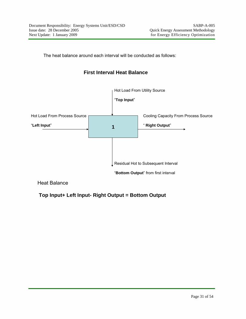
The heat balance around each interval will be conducted as follows:

1

First Interval Heat Balance

Hot Load From Utility Source

“Top Input”

Hot Load From Process Source

“Left Input”

Cooling Capacity From Process Source

“ Right Output”

Residual Hot to Subsequent Interval

“Bottom Output” from first interval

Heat Balance

Top Input+ Left Input- Right Output = Bottom Output


Page 32 of 54

1

Numerical Example of First Interval Heat Balance

Hot Load From Utility Source

“Top Input”= 0.0 kW


“Left Input”= 0.0 kW


“ Right Output”=760 kW


“Bottom Output” from first interval

Heat Balance

Top Input+ Left Input- Right Output = Bottom Output0.0 + 0.0 - 760 = - 760 kW

= - 760 kW


Page 33 of 54

N

Subsequent Intervals Heat Balance

Hot Load From Above Interval

“Top Input”


“Left Input”


“ Right Output”


“Bottom Output”

Heat Balance

Top Input+ Left Input- Right Output = Bottom Output


Page 34 of 54

2

Numerical Example for Subsequent Intervals Heat BalanceFor instance; Interval # 2

Hot Load From Above Interval

“Top Input” = -760


“Left Input”= 1300


“ Right Output”= 2470


“Bottom Output” = - 1930

Heat BalanceTop Input+ Left Input- Right Output = Bottom Output- 760 + 1300 -2470 = -1930


Page 35 of 54

Upon the completion of heat balance around each interval the following diagram will be produced:

Thermal Cascade Diagram (Un-Balanced)

Note: During this step the input from Hot Utility to the first interval is equal to zero

0.0

1300

- 2620

-2340

- 2040

- 1930

- 760

0.0

2470

760

100 210

750 1050

100 380

50 0.06

5

4

3

2

1

- 2570

The maximum difference between the available hot loads and cooling capacities from the heat balances of these intervals is – 2620 kW. This deficiency in heat will be supplied via outside hot utility.


Page 36 of 54

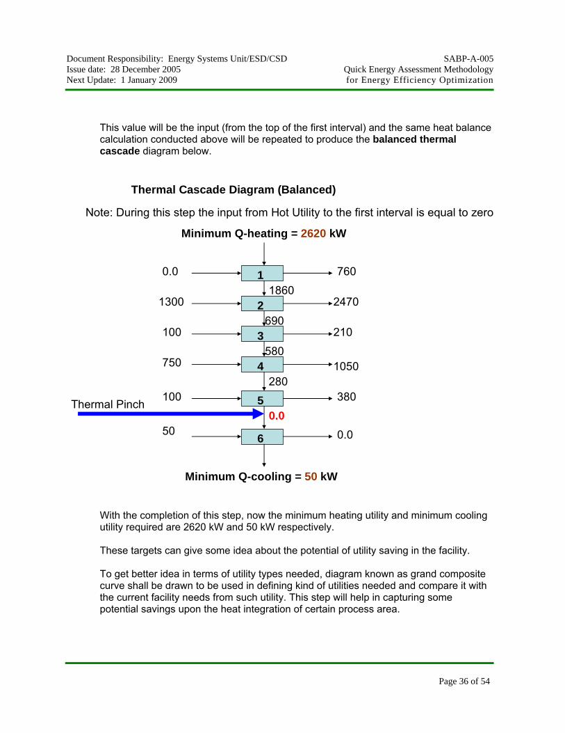
This value will be the input (from the top of the first interval) and the same heat balance calculation conducted above will be repeated to produce the balanced thermal cascade diagram below.

Thermal Cascade Diagram (Balanced)

Note: During this step the input from Hot Utility to the first interval is equal to zero

0.0

1300

0.0

280

580

690

1860

Minimum Q-heating = 2620 kW

2470

760

100 210

750 1050

100 380

50 0.06

5

4

3

2

1

Thermal Pinch

Minimum Q-cooling = 50 kW With the completion of this step, now the minimum heating utility and minimum cooling utility required are 2620 kW and 50 kW respectively. These targets can give some idea about the potential of utility saving in the facility. To get better idea in terms of utility types needed, diagram known as grand composite curve shall be drawn to be used in defining kind of utilities needed and compare it with the current facility needs from such utility. This step will help in capturing some potential savings upon the heat integration of certain process area.


Page 37 of 54

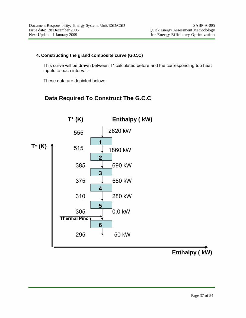
4. Constructing the grand composite curve (G.C.C)

This curve will be drawn between T* calculated before and the corresponding top heat inputs to each interval. These data are depicted below:

Data Required To Construct The G.C.C

0.0 kW

280 kW

580 kW

690 kW

1860 kW

2620 kW

6

5

4

3

2

1

Thermal Pinch

50 kW

385

375

310

305

295

515

555

T* (K) Enthalpy ( kW)

T* (K)

Enthalpy ( kW)


Page 38 of 54

Drawing these data as T* versus Enthalpy results in the following diagram that can be used to define different levels of utilities that can be used to satisfy the process heating utility requirement as shown below.

Grand Composite Curve (G.C.C)Should Be Drawn To Scale

T* (K)

Enthalpy ( kW)

700 1400 2100 2800200

300

400

500

600

Total hot utility required is equal to 2620 kW

Hu1

Hu2Hu3


Page 39 of 54

Multiple utility targeting/selection using Grand Composite Curve (GCC) Upon maximizing heat recovery in the heat exchanger network, those heating duties and cooling duties not serviced by heat recovery must be provided by external utilities. The most common utility is steam. It is usually available at several levels. High temperature heating duties require furnace flue gas or a hot oil circuit. Cold utilities might be refrigeration, cooling water, air cooling, furnace air preheating, boiler feed water preheating, or even steam generation at higher temperatures. Although the composite curves can be used to set energy targets, they are not a suitable tool for the selection of utilities. The grand composite curve drawn above is a more appropriate tool for understanding the interface between the process and the utility system. It is also as will be shown in later chapters a very useful tool in studying of the interaction between heat-integrated reactors, separators and the rest of the process. The GCC is obtained via drawing the problem table cascade as we shown earlier. The graph shown above is a typical GCC. It shows the heat flow through the process against temperature. It should be noted that the temperature plotted here is the shifted temperature T* and not the actual temperature. Hot streams are represented by ∆Tmin/2 colder and the cold streams ∆Tmin/2 hotter tan they are in the streams problem definition. This method means that an allowance of ∆Tmin is already built into the graph between the hot and the cold for both process and utility streams. The point of “zero” heat flow in the GCC is the pinch point. The open “jaws” at the top and the bottom represent QHmin and QCmin respectively. The grand composite curve (GCC) provides convenient tool for setting the targets for the multiple utility levels of heating utilities as illustrated above.


Page 40 of 54

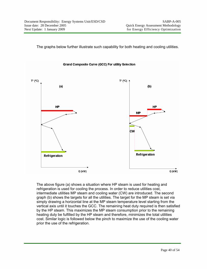
The graphs below further illustrate such capability for both heating and cooling utilities.

The above figure (a) shows a situation where HP steam is used for heating and refrigeration is used for cooling the process. In order to reduce utilities cost, intermediate utilities MP steam and cooling water (CW) are introduced. The second graph (b) shows the targets for all the utilities. The target for the MP steam is set via simply drawing a horizontal line at the MP steam temperature level starting from the vertical axis until it touches the GCC. The remaining heat duty required is then satisfied by the HP steam. This maximizes the MP steam consumption prior to the remaining heating duty be fulfilled by the HP steam and therefore, minimizes the total utilities cost. Similar logic is followed below the pinch to maximize the use of the cooling water prior the use of the refrigeration.


Page 41 of 54

The points where the MP steam and CW levels touch the GCC are called utility pinches since these are caused by utility levels. The graph (C) below shows a different possibility of utility levels where furnace heating is used instead of HP steam. Considering that furnace heating is more expensive than MP steam, the use of the MP steam is first maximized. In the temperature range above the MP steam level, the heating duty has to be supplied by the furnace flue gas. The flue gas flowrate is set as shown in graph via drawing a sloping line starting from the MP steam to theoretical flame temperature Ttft. If the process pinch temperature is above the flue gas corrosion temperature, the heat available from the flue gas between the MP steam and pinch temperature can be used for process heating. This will reduce the MP steam consumption. In summary, the GCC is one of the basic tools used in pinch technology for the selection of appropriate utility levels and for targeting for a given set of multiple utility levels. The targeting involves setting appropriate loads for the various utility levels by maximizing cheaper utility loads and minimizing the loads on expensive utilities.


Page 42 of 54

MP

CW

Refrigeration

T*

H

T-tft(C)


Page 43 of 54

Normally, Plant’s Operations have choices of many hot and cold utilities and the graph below shows some of available options. Generally, it is recommended to use hot utilities at the lowest possible temperature while generating it at the highest possible temperature. And for the cold utilities it is recommended to use it at the highest possible temperature and generate at the lowest possible temperature. These recommendations are best addressed systematically using the grand composite curve.

ProcessHeatPump

Boiler HouseAnd Power Plant

Hot OilCircuit

Furnace

Fuel

Cooling Towers

Refrigeration

Steam Turbines

Gas Turbines

Air preheat

W

W

W

W

BFWpreheat

Hot and cold utilities


Page 44 of 54

Understanding the Grand Composite Curve: The graph below shows that utility pinches are formed according to the number of utilities used. Each time a utility is used a “utility pinch” is created. It also shows that the GCC right noses sometimes known as “pockets” are areas of heat integration/energy recovery. In other words it does not need any external utilities. These right noses/pockets are caused by;

- Region of net heat availability above the pinch

- Region of net heat requirement below the pinch


Page 45 of 54

Applying the Grand Composite Curve: GCC curve can be used by engineers to select the best match between utility profile and process needs profile. For instance, the steam system shown below needs to be integrated with the process demands profile to minimize low pressure steam flaring and high or medium pressures steam let downs. Besides it helps selecting steam header pressure levels and loads.

chemicals

Proc. #1

Proc. #1

Proc. #1

Proc. #2

Proc. #3

Proc. #4





Process Condensate

HP Boiler

MP Boiler

HP

MP

LP

Vent

Effluent

Deaerator

Vent


Page 46 of 54

T

H

CW

BFW

LP

HP

MP

Superimposed Utility Profile with Process ProfileNominal Case Supply-Demand Matching Problem

Process GCC

The superimposed steam system on the process grand composite curve shows that while process heating needs can be achieved electricity can also be generated to satisfy process demands and/or export the surplus to the grid.


Page 47 of 54

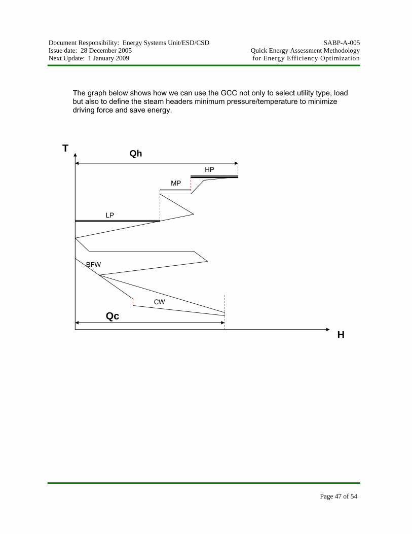
The graph below shows how we can use the GCC not only to select utility type, load but also to define the steam headers minimum pressure/temperature to minimize driving force and save energy.

T

H

CW

BFW

LP

MP

HP

Qh

Qc


Page 48 of 54

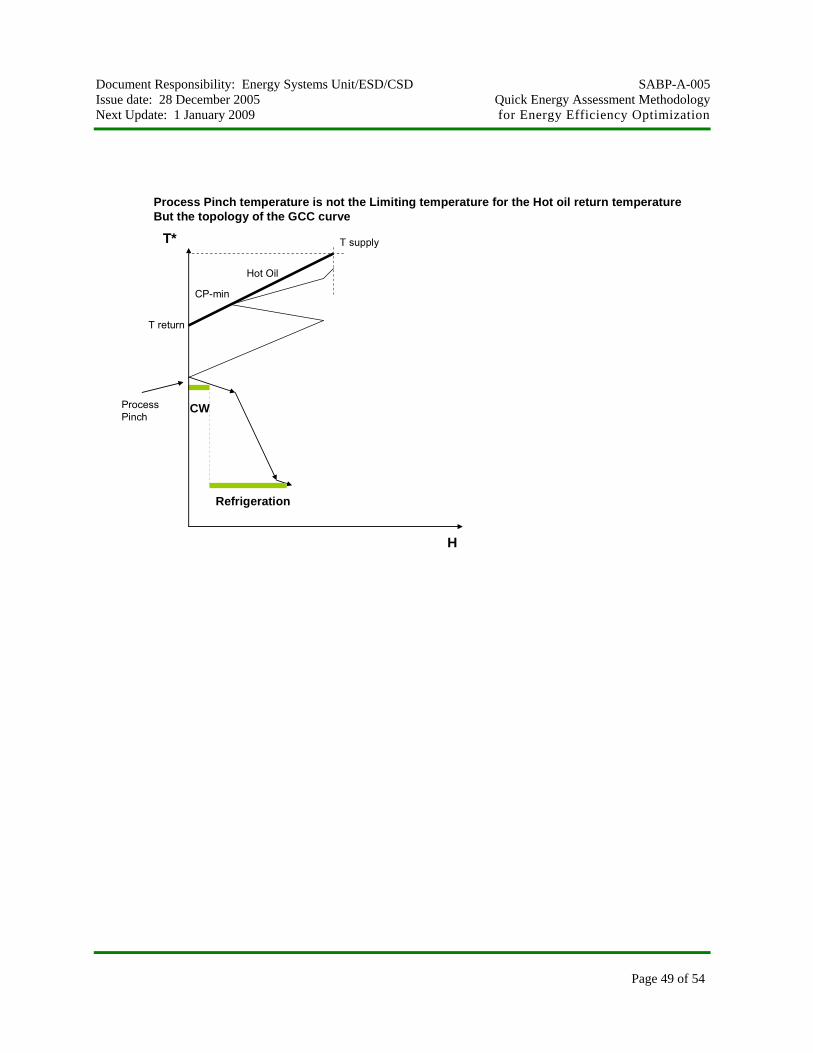
Grand Composite Curve can also be utilized to select the load and return temperature of hot oil circuits. The graph below shows that while in many cases the process pinch can be our limiting point in defining the load (slop of the hot oil line) and the return temperature of the heating oil. In some other cases the topology of the GCC is the limiting point not the process pinch. This is also shown in the second graph below. This practical guide to select the load and the target temperature of the hot oil circuits is also applicable to furnaces as will be shown later in this chapter.

CW

Refrigeration

T*

H

Process Pinch

Hot Oil

T return

T supply

Process Pinch temperature is the Limiting temperature for the Hot oil return temperature


Page 49 of 54

CW

Refrigeration

T*

H

Process Pinch

Hot Oil

T return

T supply

Process Pinch temperature is not the Limiting temperature for the Hot oil return temperatureBut the topology of the GCC curve

CP-min


Page 50 of 54

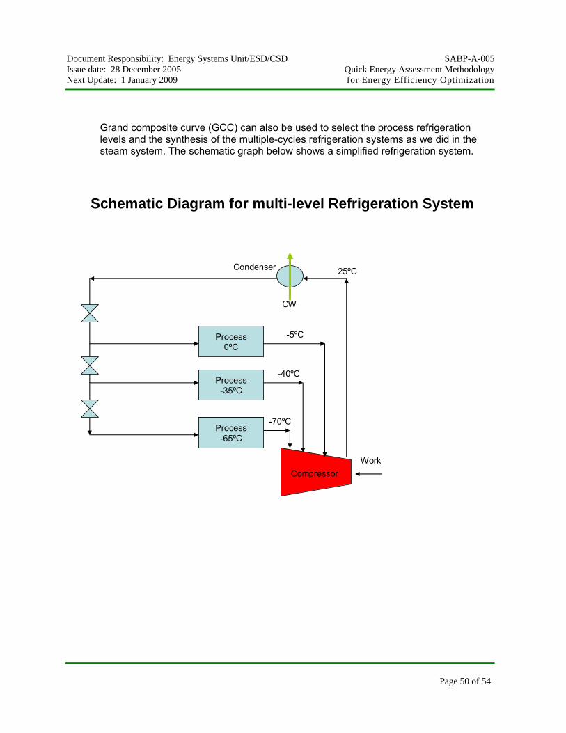
Grand composite curve (GCC) can also be used to select the process refrigeration levels and the synthesis of the multiple-cycles refrigeration systems as we did in the steam system. The schematic graph below shows a simplified refrigeration system.

Schematic Diagram for multi-level Refrigeration System

Work

Process0ºC

CW

Process-35ºC

Process-65ºC

25ºC

-5ºC

-40ºC

-70ºC

Compressor

Condenser


Page 51 of 54

The GCC as we mentioned before can be used to place the refrigeration levels as we did with steam levels. The graph below shows how we can do that.

T

H

Tcw

We can place the refrigeration levels like steam levels.Maximizing the highest temperature load to minimize the lower temperature loads

- 5 ºC

- 40 ºC

- 70 ºC


Page 52 of 54

When a hot utility needs to be at a high temperature and/or provide high heat fluxes, radiant heat transfer is used from combustion of fuel in furnace. Furnace designs vary according to the function of the furnace, heating duty and type of fuel, and method of introducing combustion air.

4A.3 Basic Formulas for Some Quick Savings Estimation _Compression Energy % Savings Due to Decrease in compressors Inlet temperature % Energy saving in a compressor energy consumption = {1- (Tnew/Told)} * 100 Tnew is the new inlet temperature

Told is the old inlet temperature _ Turbines gland steam leakage: Steam leakage in kg/hr = Flow of steam measured- Flow of steam

utilized/required Flow of steam required= work shaft required/ {Estimated Isentropic efficiency*(Inlet

enthalpy- outlet isentropic enthalpy) Outlet isentropic enthalpy can be obtained from steam tables knowing outlet isentropic entropy and outlet temperature or pressure Outlet isentropic entropy = inlet entropy Inlet entropy can be obtained from steam tables at inlet temperature and pressure _ Back pressure turbines energy available for integration Thermal energy available for Integration (Q) = Outlet steam flow*

(Vapor enthalpy- liquid enthalpy) Outlet steam flow= Inlet steam flow (1- actual wetting factor) Actual wetting factor can be assumed between (8 to 15) % _ % Energy saving in heat pumps/refrigeration cycles due to decrease in reject

temperature


Page 53 of 54

W2/W1 = (T reject 2 – Tc)/ (T reject 1 – Tc) Treject is the temperature at which heat is rejected to the cooling medium (water) Tc is the temperature at which heat is taken into the refrigeration) cycle _ Material balance for the cooling tower Assuming the system is at equilibrium Make-up = Evaporation+ Blowdown+ Windage loss Cooling towers cycles of concentration (C) C= concentration of solids in the circulating water/ concentration of solids in

make-up water _ Energy saving in adjusting of combustion in a natural gas fired boiler/furnace Analysis on the exhaust from the boilers sometimes or most of the times in some places reveals excess oxygen levels which result in unnecessary energy consumption. This excess air defines a low efficiency on the combustion process. Portable or even on-line flue gas analyzer can be used as a part of a rigorous boilers/furnaces inspection program. The optimum amount of O2 in the flue gas of a gas fired boiler is 2%, which corresponds to 10% excess air. Controlling the combustion process could lead to at least 2% fuel saving upon bringing the excess O2 from for instance 6% to 2%. Cost saving $/year= Energy usage per year* % possible fuel savings* fuel cost

per unit of energy Energy saving in adjusting of combustion in a an oil fired boiler/furnace. Analysis on the exhaust from the boilers sometimes or most of the times in some places reveals excess oxygen levels which result in unnecessary energy consumption. This excess air defines a low efficiency on the combustion process. Portable or even on-line flue gas analyzer can be used as a part of a rigorous boilers/furnaces inspection program. The optimum amount of O2 in the flue gas of an oil fired boiler is 4%. Controlling the combustion process could lead to at least 1% fuel saving upon bringing the excess O2 from for instance 6% to 1%.


Page 54 of 54

Cost saving $/year= Energy usage per year* % possible fuel savings* fuel cost

per unit of energy Energy saving in preheating boiler/furnace combustion air with stack’s waste heat: If the intake air (air drawn from outside into the natural gas boiler) is at ambient outdoor temperature unnecessary fuel will be consumed to heat up this combustion air. In order to reduce fuel consumption, it is recommended to install recuperative air pre-heater on the air intake of the boiler to preheat combustion air using heat which is exhausted along with the combustion from the boiler. Stack exhaust losses are part of all fuel-fired processes. They increase with the exhaust temperature and the amount of excess air the exhaust contains. A high quality air pre-heater could recover more than 40% of this waste heat. Therefore, the potential savings from the installation of air pre-heater on the boiler is: Cost saving = fuel cost ($)/unit of energy* Energy Consumed/year*(boiler

efficiency)*percent of energy recovered by air pre-heater Note: The following attached pages are two curves and a table that can be used to

estimate the percentage of fuel savings.

4A.4 HGP Detailed Energy Assessment Study Final Report, SAER # 5995,”Detailed Energy Assessment at Hawiyah Gas Plant”, June 26, 2005

Documents

SABP-A-005