s3.amazonaws.coms3.amazonaws.com/zanran_storage/ 1 Introduction 1 1.1 The Scope of Macroeconomics . . . . . . . . . . . . . . . . . . . . 1 1.2 US Macroeconomic Data: A Helicopter

Intermediate Macroeconomics

Dirk Krueger1 Department of EconomicsUniversity of Pennsylvania

April 2007

1 I would like to thank Charles Jones, Felix Kubler, Beatrix Pall and Tom Sargentfor stimulating discussions about teaching modern macro. All remaining errors aremine.

ii

Contents

1 Introduction 11.1 The Scope of Macroeconomics . . . . . . . . . . . . . . . . . . . . 11.2 US Macroeconomic Data: A Helicopter Tour . . . . . . . . . . . 2

1.2.1 Real GDP . . . . . . . . . . . . . . . . . . . . . . . . . . . 21.2.2 Digression: The Rest of the Course . . . . . . . . . . . . . 31.2.3 Other Macroeconomic Aggregates . . . . . . . . . . . . . 6

2 National Income and Product Accounting (NIPA) 112.1 Gross Domestic Product (GDP) . . . . . . . . . . . . . . . . . . . 11

2.1.1 Computing GDP through Production . . . . . . . . . . . 122.1.2 Computing GDP through Spending . . . . . . . . . . . . 132.1.3 Computing GDP through Income . . . . . . . . . . . . . . 16

2.2 Price Indices . . . . . . . . . . . . . . . . . . . . . . . . . . . . . 192.3 From Nominal to Real GDP . . . . . . . . . . . . . . . . . . . . . 202.4 Measuring In�ation . . . . . . . . . . . . . . . . . . . . . . . . . . 212.5 Measuring Unemployment . . . . . . . . . . . . . . . . . . . . . . 222.6 Measuring Transactions with the Rest of the World . . . . . . . . 232.7 Appendix A: More on Growth Rates . . . . . . . . . . . . . . . . 252.8 Appendix B: Chain-Weighted GDP . . . . . . . . . . . . . . . . . 27

3 Economic Growth 333.1 Mathematical Preliminaries . . . . . . . . . . . . . . . . . . . . . 33

3.1.1 Discrete vs. Continuous Time . . . . . . . . . . . . . . . . 333.1.2 Derivatives . . . . . . . . . . . . . . . . . . . . . . . . . . 333.1.3 Some Useful Facts about Logs . . . . . . . . . . . . . . . 343.1.4 Growth Rates (once again) . . . . . . . . . . . . . . . . . 353.1.5 Growth Rates of Functions . . . . . . . . . . . . . . . . . 353.1.6 Simple Di¤erential Equations and Constant Growth Rates 36

3.2 Growth and Development Facts . . . . . . . . . . . . . . . . . . . 373.3 The Solow Model . . . . . . . . . . . . . . . . . . . . . . . . . . . 43

3.3.1 Models . . . . . . . . . . . . . . . . . . . . . . . . . . . . 433.3.2 Setup of the Basic Model and Model Assumptions . . . . 433.3.3 Analysis of the Model . . . . . . . . . . . . . . . . . . . . 463.3.4 Introducing Growth . . . . . . . . . . . . . . . . . . . . . 51

iii

iv CONTENTS

3.3.5 Analysis of the Extended Model . . . . . . . . . . . . . . 553.3.6 Evaluation of the Solow Model . . . . . . . . . . . . . . . 64

3.4 The Convergence Discussion . . . . . . . . . . . . . . . . . . . . . 673.5 Growth Accounting and the Productivity Slowdown . . . . . . . 723.6 Ideas as Engine of Growth . . . . . . . . . . . . . . . . . . . . . . 75

3.6.1 Technology . . . . . . . . . . . . . . . . . . . . . . . . . . 753.6.2 Ideas . . . . . . . . . . . . . . . . . . . . . . . . . . . . . . 763.6.3 Data on Ideas . . . . . . . . . . . . . . . . . . . . . . . . . 79

3.7 Infrastructure . . . . . . . . . . . . . . . . . . . . . . . . . . . . . 803.7.1 Cost of Investment . . . . . . . . . . . . . . . . . . . . . . 803.7.2 Bene�ts of Investment . . . . . . . . . . . . . . . . . . . . 81

3.8 Endogenous Growth Models . . . . . . . . . . . . . . . . . . . . . 823.9 Neutrality of Money . . . . . . . . . . . . . . . . . . . . . . . . . 863.10 Summary . . . . . . . . . . . . . . . . . . . . . . . . . . . . . . . 86

4 Business Cycle Fluctuations 894.1 Potential GDP and Aggregate Demand . . . . . . . . . . . . . . 894.2 The IS-LM Framework . . . . . . . . . . . . . . . . . . . . . . . . 92

4.2.1 The Balance of Income and Spending: Keynesian Crossand Multiplier . . . . . . . . . . . . . . . . . . . . . . . . 92

4.2.2 Investment, the Interest Rate and the IS Curve . . . . . . 1054.2.3 The Demand for Money and the LM-Curve . . . . . . . . 1094.2.4 Combination of IS-Curve and LM-Curve: Short-Run Equi-

librium . . . . . . . . . . . . . . . . . . . . . . . . . . . . 1164.2.5 Monetary and Fiscal Policy in the IS-LM Framework . . . 118

4.3 The Aggregate Demand Curve . . . . . . . . . . . . . . . . . . . 1224.4 Unemployment . . . . . . . . . . . . . . . . . . . . . . . . . . . . 123

4.4.1 Concepts and Facts . . . . . . . . . . . . . . . . . . . . . 1244.4.2 Some Theory and the Natural Rate of Unemployment . . 1264.4.3 Unemployment and the Business Cycle . . . . . . . . . . . 129

4.5 The Price Adjustment Process . . . . . . . . . . . . . . . . . . . 1324.5.1 Aggregate Demand, Potential GDP and the Price Adjust-

ment Process . . . . . . . . . . . . . . . . . . . . . . . . . 1364.5.2 Monetary Policy . . . . . . . . . . . . . . . . . . . . . . . 1374.5.3 Fiscal Policy . . . . . . . . . . . . . . . . . . . . . . . . . 138

4.6 Stabilization Policy . . . . . . . . . . . . . . . . . . . . . . . . . . 1404.6.1 Aggregate Demand Shocks and Their Stabilization . . . . 1414.6.2 Price Shocks and Their Stabilization . . . . . . . . . . . . 143

4.7 Real Business Cycle Theory . . . . . . . . . . . . . . . . . . . . . 146

5 Microeconomic Foundations of Macroeconomics 1495.1 Consumption Demand . . . . . . . . . . . . . . . . . . . . . . . . 149

5.1.1 Data on Consumption . . . . . . . . . . . . . . . . . . . . 1495.1.2 The Keynesian Aggregate Consumption Function and the

Data . . . . . . . . . . . . . . . . . . . . . . . . . . . . . . 1515.1.3 The Life Cycle/Permanent Income Model of Consumption 153

CONTENTS v

5.2 Investment Demand . . . . . . . . . . . . . . . . . . . . . . . . . 1685.2.1 Facts about Investment . . . . . . . . . . . . . . . . . . . 1685.2.2 The Theory of Investment . . . . . . . . . . . . . . . . . . 171

6 Trade, Exchange Rates & International Financial Markets 1776.1 Terms of Trade, the Nominal and the Real Exchange Rate . . . . 1776.2 E¤ects of the Real Exchange Rate on the Trade Balance . . . . . 1806.3 Determinants of the Real Exchange Rate . . . . . . . . . . . . . . 181

6.3.1 Purchasing Power Parity . . . . . . . . . . . . . . . . . . . 1816.3.2 Real Exchange Rates and Interest Rates . . . . . . . . . . 184

6.4 The International Financial System . . . . . . . . . . . . . . . . . 185

7 Fiscal and Monetary Policy in Practice 1877.1 Fiscal Policy . . . . . . . . . . . . . . . . . . . . . . . . . . . . . 187

7.1.1 Data on Fiscal Policy . . . . . . . . . . . . . . . . . . . . 1877.1.2 A Few Theoretical Remarks . . . . . . . . . . . . . . . . . 195

7.2 Monetary Policy . . . . . . . . . . . . . . . . . . . . . . . . . . . 197

vi CONTENTS

Chapter 1

Introduction

1.1 The Scope of Macroeconomics

Macroeconomics wants to explain the evolution of the main economic aggregatesover time. We are interested in why total production (real GDP) grows over timeon average and why it shows sizeable �uctuations around its long-run growthtrend. We want to understand what causes unemployment and in�ation, howinterest rates behave and what causes a trade de�cit.In contrast to microeconomics, where the object of interest is a single �rm

or household, in macroeconomics we study the whole economy. Our reason-ing, however, will be based on the insights that microeconomic theory provides(therefore the prerequisite requirements for this course).Why should we care about macroeconomics. I could think of three good

reasons

1. It a¤ects us on a day-to-day basis: A rise in the interest rate makes loansfor cars more expensive, raises the interest rate that you pay on a mortgageand (usually) has a negative e¤ect on stock prices. A decline in productionleads to people being laid o¤ -and that could be a member of your family.High in�ation wipes out part of the value of your savings. The list goeson and on....

2. A good understanding of macroeconomics is essential for policy makers.Politicians can change �scal policy (how much the government spendsand how much it taxes you) and central bankers (Alan Greenspan and hisFederal Reserve Board) can change monetary policy (how much currencyto issue and how high to set the Federal Funds Rate -an important interestrate). As we will see later �scal and monetary policy can have good andbad e¤ects on the economy. It is crucial that policy makers and centralbankers understand macroeconomic data and macroeconomic theory tomake an informed decision about when and to what extent to changemonetary and �scal policy.

1

2 CHAPTER 1. INTRODUCTION

3. A good understanding is important for us as good citizens because it helpsus to understand and critic what politicians, central bankers and the presstell us about the economy and what should be done to improve it.

But let�s �rst look at some data to see what it is that we�re talking about,or, to speak with Sherlock Holmes

Data! Data! Data! I can�t make bricks without clay.

1.2 USMacroeconomic Data: AHelicopter Tour

1.2.1 Real GDP

When economists say that the US economy grew 2% last year they usually mean:real Gross Domestic Product (GDP) was 2% higher in 2000 than in 1999. Letus �rst de�ne what nominal GDP is.

De�nition 1 Nominal GDP is the total value of goods and services producedin an economy during a particular time period.

Note that when talking about GDP we have to specify the GDP of whateconomy (e.g. the US) for what time period (e.g. a year, say 2000) we mean.Nominal GDP is measured in dollars. Since prices tend to increase over time(ask your parents how much college tuition cost 30 years ago), so will nominalGDP. To measure the economic activity of a country we are really interestedin how many real goods and services were produced in the economy. This ismeasured by real GDP.

Real GDP =Nominal GDPPrice Level

We will discuss how to compute the �Price Level�in the next section. Finally,a growth rate of a variable is computed as follows. Let Yt denote real GDP inperiod t (i.e. Y2000 is real GDP for the year 2000). Then the growth rate of realGDP from period t� 1 to period t is computed as

gY (t� 1; t) =Yt � Yt�1Yt�1

As an example, suppose real GDP in 1988 equals $ 585 and $ 605 in 1989, thenthe growth rate of real GDP between 1988 and 1989 would equal

gy(1988; 1989) =$605� $585

$585= 0:034 = 3:4%

This is the number that people mean when they say that the economy grew by3:4% in 1989.

1.2. US MACROECONOMIC DATA: A HELICOPTER TOUR 3

Let�s look at some data for real GDP. The solid line in Figure 1 shows theevolution of real GDP for the US economy from 1967 to 2001.1 We have twoprincipal observations

1. Real GDP grows over time. If GDP would have grown at 2.75%, then thegraph of real GDP would have looked like the dotted line. The dotted lineis called �Trend�, because it shows how real GDP evolved on average.

2. Actual real GDP exhibits -occasionally sizeable- deviations from its longterm growth trend. These �uctuations are called business cycles.

Figure 2 shows these �uctuations in more detail. The dotted line at 0 corre-sponds to the trend. When the solid line takes the value -0.061 as in 1983, thismeans that actual real GDP was 6.1% below the trend.

Periods in which real GDP actually declines are called recessions, and, ifthese declines are extremely severe, depressions.2 From 1967 until 2001 the USexperienced 5 recessions.3 Note that, although recessions are recurrent events,the exact timing of a recession is extremely hard to forecast.

1.2.2 Digression: The Rest of the Course

At this stage let�s have a short preview of the course. The two main sections,Sections 3 and 4 deal exactly with the two observations we made about Figure1:In Section 3 we will study why, on average, the economy grows over time.

This area of study is called growth theory and we will discuss the neoclassicalgrowth model. As a sneak preview, the economy grows over time because:

1The data have quarterly frequency, i.e. there one observation for real GDP for each quar-ter. The �rst observation is the GDP for the �rst three months of 1967, the last observationis the GDP for April to June 2001. The data are then converted to yearly numbers (ba-sically by multiplying them by 4). If you are interested in the actual data, on the WWWgo to http://www.economagic.com/em-cgi/data.exe/fedstl/gdp96+1#DataWhat is actuallyplotted is the natural logarithm of real GDP, for the following reason. If GDP grows at aconstant rate g; then the log of GDP is a straight line with slope g: By plotting the log ofGDP we can draw the long-term growth trend as a straight line (rather than an exponentialfunction). This technique is used quite often by economists. Hall and Taylor plot GDP in-stead of log GDP, but use a logarithmic scale on the y-axis on p. 6 (observe that the distancebetween 3500 and 4000 is bigger than between 6000 and 6500 on the y-axis; this is what alog-scale does). Both tricks are equivalent.

2The US economy as well as other economies in the world experienced a depression, theso-called great depression, from 1929 to 1932.

3One de�nition of a recession is �a decline in two subsequent quarters of real GDP�. Ifyou are interested in more detailed information about the timing and length of expansionsand recessions, visit the webpage of the National Bureau of Economic Research (NBER) athttp://www.nber.org/cycles.html. Note that, according to the o¢ cial de�nition of a recession,the U.S. economy is not currently in a recession, as real GDP growth has not been negativein the �rst two quarters of 2001.


1970 1975 1980 1985 1990 1995 20008

8.2

8.4

8.6

8.8

9

9.2Real GDP in the United States 19672001

Year

Log

of re

al G

DP

GDP

Trend

1. the population grows. A higher population means that a bigger labor forceis available for the production of goods and services.

2. more capital is accumulated. Over time, more and more machines andother equipment are used in the production process

3. there is technological progress (e.g. the development of faster and fastercomputer chips) makes capital and labor more productive in the produc-tion process.

In Section 4 we will study why there are business cycles, i.e. why the economy�uctuates around its long-term growth trend. In contrast to growth theory,where the level of agreement between economists is fairly high, in business cycletheory there is substantial disagreement about why business cycles exist andwhat the government can do about them. Again a brief sneak preview:

1. in this course we mostly will follow Hall and Taylor (and many others)and assume that in the short run wages and/or prices are �sticky�, i.e. not


1970 1975 1980 1985 1990 1995 20000.08

0.06

0.04

0.02

0

0.02

0.04

0.06

0.08Expansions and Recessions

Year

Perc

enta

ge D

evia

tion

of R

eal G

DP fr

om T

rend

197071recession

197475recession

198082backtoback recessions

199091recession

�exible to adjust immediately to shocks hitting the economy. Potentialshocks could come from the private sector of the economy (a certain dropof households�willingness to buy cars), from world markets (rememberthe oil price shocks in 1973 and 1980) or from changes in monetary and�scal policy. The results are business cycles.

2. an alternative view holds that business cycles originate from �technologyshocks� (e.g. in certain years we have bad weather and that makes pro-duction, in particular agricultural production, more di¢ cult). Prices andwages are fully �exible even in the short run. People respond optimallyand work more when the conditions are such that they are productive (inyears of good technology shocks) and less when they are not so productive.Hence in good years workers supply a lot of labor and production (realGDP) is high, in years with bad technology workers supply little laborand real GDP is low. This view has become known as �Real BusinessCycle Theory�(�Real�because the shocks underlying business cycles are


technology shocks).4

The dispute between these two schools is not only theoretical. Based ontheory, economists from both camps have di¤erent views about economic pol-icy. In RBC-theory business cycles arise because households react optimallyto technology shocks. Hence there is no role for government policy to improvematters. If business cycles come about because prices and wages can�t adjust inthe short run (as in the �rst view), there may be a role for an active monetaryand �scal policy to reduce the economic �uctuations.Common among both schools is that they both use models -abstract simple

descriptions of the economy, either with equations or graphs- to explain busi-ness cycles and to argue for or against a certain policy. We will follow thismethodological approach.

1.2.3 Other Macroeconomic Aggregates

Why are business cycles bad? Because if real production declines, workers getlaid o¤ and the unemployment rate increases. We should expect that theunemployment rate follows the path of real output rather closely. Let us �rstde�ne the unemployment rate.

De�nition 2 The labor force is the number of people, 16 or older, that areeither employed or unemployed but actively looking for a job. The unemploymentrate is given by

Unemployment Rate =number of unemployed people

labor force

In Figure 3 we plot the unemployment rate for the US from 1967 to 2001.5

We see that in recessions the unemployment rate increases, whereas in expansionit decreases. A variable that shows such a behavior is called �countercyclical�:it is high when real GDP is low (relative to trend) and it is low when real GDPis high. Also note that currently unemployment is at its lowest level since 1970.

Another important macroeconomic variable is the in�ation rate. It mea-sures the growth rate of the price of a particular basket of goods and services.6

Let Pt be the price level in period t: Then the in�ation rate between periodst� 1 and t is given by

�t = gP (t� 1; t) =Pt � Pt�1Pt�1

4The founders of RBC-theory are Finn Kydland from Carnegie Mellon University and EdPrescott from the University of Minnesota -incidentally my Ph.D. thesis advisor.

5The unemployment rate is measured by the Bureau of Labor Statistics (BLS). Go to theirhomepage at http://stats.bls.gov/top20.html if you want to have a look at the original data.

6There are several measures of the in�ation rate. They are distinguished by what goodsand services are included in the basket of goods whose price is measured. The two mostimportant indexes for in�ation are the Consumer Price Index (CPI) and the GDP de�ator.Both will be discussed in the next section.


1970 1975 1980 1985 1990 1995 20002

3

4

5

6

7

8

9

10

11

12Unemployment Rate for the US 19672001

Year

Une

mpl

oym

ent R

ate

197071recession

197475recession


199091recession

Figure 4 shows the in�ation rate for the US economy from 1967 to 2001.We see that in�ation rates were higher and more volatile in the 70�s and early80�s than in the 90�s. Combining �gure 2 and 4 it is not apparent whether thein�ation rate is procyclical or countercyclical.

Interest Rates are important macroeconomic variables because they de-termine how costly it is to take out a loan to buy a car, a house, stocks, or, for�rms, to �nance new equipment. How are interest rates computed. Suppose inperiod t � 1 you borrow the amount $Bt�1. The loan speci�es that in periodt you have to repay $Bt: In general $Bt will be bigger than Bt�1 (since youhave to repay Bt�1; the so-called principal, and the interest on the loan): Thenominal interest rate on the loan from period t� 1 to period t, it; is computedas

it =Bt �Bt�1Bt�1


1970 1975 1980 1985 1990 1995 20000

2

4

6

8

10

12

14

16Inflation Rate for the US 19672001

Year

Infla

tion

Rat

e

This is called a nominal interest rate because it does not take into accountin�ation. The real interest rate rt is de�ned as the di¤erence between thenominal interest rate and the in�ation rate:

rt = it � �t

Note that nominal interest rates historically tend to rise with in�ation: lendersdemand a higher nominal interest rate in times of high in�ation as compensationfor the loss of purchasing power of their money, due to high in�ation.Example: In the year 2000 you borrow $15; 000 to buy a new car and the

bank asks you to repay $16; 500 exactly one year later. Then the yearly nominalinterest rate from 2000 to 2001 is

i2001 =$16; 500� $15; 000

$15; 000= 0:1 = 10%

Now suppose the in�ation rate is 3% in 2001. Then the real interest rate equals10%� 3% = 7%


Note that whenever stating an interest rate, it is crucial to state the lengthof the period with respect to which it applies, i.e. whether it is a yearly, aquarterly, a monthly or a daily interest rate.In Figure 5 the nominal interest rate for the US economy from 1967 to 2001

is plotted.7 Comparing Figure 2 and Figure 5 indicates that interest rates tendto be procyclical: they increase during expansions and fall during recessions.

1970 1975 1980 1985 1990 1995 20000

2

4

6

8

10

12

14

16

18

20Federal Funds Interest Rate 19672001

Year

Nom

inal

Inte

rest

Rat

e in

%

Now we have a rough idea about how the most important macroeconomicvariables evolved over the last 30 years. Now we turn to a discussion how thesevariables are actually measured in the data.

7There are many di¤erent interest rates. The Federal Funds rate is the interestrate that banks charge each other for loans from one evening to the next morning.So this is a daily interest rate. This daily interest rate has been converted into ayearly interest rate by �multiplying� the daily rate by 365. For the original data go tohttp://www.stls.frb.org/fred/data/irates.html.


Chapter 2

National Income andProduct Accounting(NIPA)

In this section we look in detail at how the macroeconomic aggregates whosebehavior over the last thirty years we studied in the last section are de�ned andmeasured in the data. We will start with gross domestic product (GDP).

2.1 Gross Domestic Product (GDP)

We de�ned nominal and real GDP in the last section. Now will we discuss howwe measure these entities in the data. Nominal GDP can be measured in threedi¤erent ways which all lead to the same result:1

1. We can measure nominal GDP by adding together the value of productionin all di¤erent industries in the economy.

2. We can measure nominal GDP by adding together the spending on goodsand services of the di¤erent sectors of the economy (households, �rms, thegovernment and foreigners).

3. We can measure nominal GDP by adding together all the income that isgenerated from the production process: wages, salaries and pro�ts.

In fact, the Bureau of Economic Analysis (BEA), the US government agencythat is responsible for measuring GDP, does calculate GDP in these three dif-ferent ways and makes sure that the three numbers they get coincide (as theyshould according to accounting principles).

1The fact that the total value of production always equals the total value of spending andalways equals the total income is called an identity, it is inevitably true as a consequence ofaccounting principles.

11

12CHAPTER 2. NATIONAL INCOMEAND PRODUCTACCOUNTING (NIPA)

2.1.1 Computing GDP through Production

We want to calculate nominal GDP by adding together the value of productionfor all di¤erent industries in the economy, agriculture, mining, construction,manufacturing etc. Can we just add together all those industries�sales? Con-sider the following example: US steel produces a ton of steel and sells it toGM for $1500. GM then uses this steel to build a car that it sells for $10,000.Assume for the moment that a car can be produced only with steel and labor.Should the contribution to GDP be the whole $11,500, the sum of total sales?No, since the steel has been counted double; once when it was sold from US

Steel to GM and once when it, as a part of the car, was sold by GM. But itwas only produced once, so we should only count it once. This is achieved bythe concept of value added. It basically measures how much a �rm, in itsproduction process, added to the value of the intermediate goods it purchasedfrom its suppliers. Roughly, value added of a �rm equals its revenues from salesminus the purchases of intermediate goods -goods that the �rm bought fromother �rms and used to produce its own products.For the example then, the contribution should be only $1500 (from the sale

of steel to GM, the value added of US Steel) plus $8500 (the value added ofGM, equal to the total sale of $10,000 minus the purchase of the intermediategood steel for $1,500).So when we measure nominal GDP through production, we sum up the

value added of all industries in the economy, because the value added (andnot the sales) are the correct contributions of the industries to production. Table1 shows the contribution of di¤erent industries to nominal GDP for 1999. Thenumbers in column 2 are in billions of dollars.2

Table 1Industries Value Added in % of Tot. Nom. GDP

Total Nom. GDP 9,299.2 100.0%Agriculture, Forestry, Fishing 125.4 1.3%Mining 111.8 1.2%Construction 416.4 4.5%Manufacturing 1,500.8 16.1%Transportation, Publ. Utilities 779,6 8.4%Wholesale Trade 643.3 6.9%Retail Trade 856.4 9.2%Finance, Insurance, Real Estate 1,792.1 19.3%Services 1,986.9 21.4%Government 1,158.4 12.5%Statistical Discrepancy -71.9 -0.8%

Note that total nominal GDP in 1999 was $US 9,299.2 billion, or $US9,299,200,000,000. To make this number a little less intimidating, economists

2All data in this section come from the Economic Report of the President (2001).

2.1. GROSS DOMESTIC PRODUCT (GDP) 13

often report GDP per capita. On average in 1999 the population of the US was275,372,000. Hence GDP per capita in 1999 amounted to $33,769.59. In 1999every person in the US, from the newborns to the old, produced on averageabout $34,000 worth of goods and services.

2.1.2 Computing GDP through Spending

Nominal GDP can also be computed by summing up the total spending ongoods and services by the di¤erent sectors of the economy. Formally, let

C = Consumption

I = (Gross) Investment

G = Government Purchases

X = Exports

M = Imports

Y = Nominal GDP

ThenY = C + I +G+ (X �M)

Let us turn to a brief description of the components of GDP:

� Consumption (C) is de�ned as spending of households on all goods, suchas durable goods (cars, TV�s, Furniture), nondurable goods (food, cloth-ing, gasoline) and services (massages, �nancial services, education, healthcare). The only form of household spending that is not included in con-sumption is spending on new houses.3 Spending on new houses is includedin �xed investment, to which we turn next.

� Gross Investment (I) is de�ned as the sum of all spending of �rms on plant,equipment and inventories, and the spending of households on new houses.It is broken down into three categories: residential �xed investment(the spending of households on the construction of new houses), non-residential �xed investment (the spending of �rms on buildings andequipment for business use) and inventory investment (the change ininventories of �rms). To make the concept of investment clearer, we haveto take a little digression about stocks and �ows.

A stock is a quantity measured at a given point in time. A �ow is a quantitymeasured per unit of time. As an example consider �lling a bathtub with water.The amount of water in the tub is a stock -we say that the bathtub contains50 gallon of water. The amount of water �owing out of the faucet is a �ow

3What about purchases of old houses? Note that no production has occured (since thehouse was already built before). Hence this transaction does not enter this years�GDP. Ofcourse, when the then new house was �rst bought by its �rst owner it entered GDP in theparticular year.


-we say that 2 gallon of water per minute �ow into the tub. Note that wemeasure the stock by gallon, the �ow by gallon per minute. Often stocks and�ows are related. In our example the stock of water in the tub equals theaccumulated �ow of water out of the faucet. The same is true with investmentand the capital stock. The capital stock of an economy is the typical economicexample of a stock, whereas investment, like GDP and its other componentsconsumption, government purchases etc. are �ow variables.4 The capital stockis the total amount of physical capital in the economy, including all buildings andequipment. Part of the capital stock wears out every period in the productionprocess, a process called depreciation (which is again a �ow variable). Wehave the following relationship between the capital stock, gross investment anddepreciation:

Capital Stock at end of this period = Capital Stock at end of last period

+Gross Investment in this period

�Depreciation in this period

We de�ne net investment as

Net Investment = Gross Investment�Depreciation

and therefore

Net Investment = Capital Stock at end of this period

�Capital Stock at end of last period

Note that what enters nominal GDP is gross, not net investment, but that netinvestment in this period equals the change of the capital stock from the end oflast to this period.What residential and nonresidential �xed investment are and why they are

included in nominal GDP is rather obvious. So let�s spend some time to un-derstand inventory investment. Suppose in 1999 Ford produces a car that youpurchase in 1999. Then your spending on the car enters GDP as consumptionunder C: But now suppose Ford produces the car and puts it in its stock forsale in 2000. Since the car is not sold yet, it doesn�t enter GDP as consumptionin 1999. But Ford�s production activity is the same, no matter whether thecar was sold or not in 1999, so the contribution to GDP should be the same.The key is inventory investment: By producing now and putting the car in itsstock, Ford increased its inventory by one car, and the statisticians count thisas investment in inventories. By the same token as before

Inventory Investment = Stock of Inventories at end of this year

�Stock of Inventories at the end of last year

Sometimes the variable �nal sales is reported in the news. (Nominal) �nalsales equal nominal GDP minus inventory investment.

4Remember the de�nition of nominal GDP: it is the total value of goods and servicesproduced in an economy during a particular time period, i.e measured in units per timeperiod.


� Government spending (G) is the sum of federal, state and local governmentpurchases of goods and services. Note that government spending does notequal total government outlays: transfer payments to households (suchas welfare, social security or unemployment bene�t payments) or interestpayments on public debt are part of government outlays, but not includedin government spending G:

� As an open economy, the US trades goods and services with the rest ofthe world. Exports (E) are deliveries of US goods and services to the restof the world, imports (M) are deliveries of goods and services from othercountries of the world to the US. Why are imports subtracted from exportswhen computing GDP. Suppose Boeing buys 4 jet engines from the Britishcompany Rolls Royce, puts them into a Boeing 747 and sells the aircraftto the French airline Air France. What has been produced in the US wasthe plane, excluding the engines. So we count the plane as exports outof the US, the engines as import into the US and the net contribution toGDP is (X�M), that is, exports minus imports. The quantity (X�M) isalso referred to as net exports or the trade balance. We say that a country(such as Germany) has a trade surplus if exports exceed imports, i.e. ifX �M > 0. A country has a trade de�cit if X �M < 0; which was thecase for the US in recent years.

In Table 2 you can see the composition of nominal GDP for 1997, brokendown to the di¤erent spending categories discussed above. Again the numbersare in billion US dollars.

Table 2in billion $ in % of Tot. Nom. GDP

Total Nom. GDP 9,299.2 100.0%Consumption 6,268.7 67.4%Durable GoodsNondurable GoodsServices

761.31,845.53,661.9

8.2%19.8%39.3%

Gross Investment 1,650.1 17.7%NonresidentialResidentialChanges in Inventory

1,203.1403.843.3

12.9%4.3%0.5%

Government Purchases 1,634.4 17.6%Federal GovernmentState and Local Government

586.61,065.8

6.3%11.5%

Net Exports -254.0 -2.7%ExportsImports

990.21,244.2

10.6%13.4%

Final Sales 9,255.9 99.5%


2.1.3 Computing GDP through Income

The production of goods and services generates income, either in the form ofwages and salaries for workers, or in the form of pro�ts for individuals runninga business. This fact provides a third way of computing nominal GDP. Thebroadest measure of the total incomes of all Americans is called national in-come. It is closely related, but not equal to nominal GDP. Remember that USGDP is the value of goods and services produced in the US. Some people inthis country are not Americans, so, although they contribute to US GDP, theirincome is not part of national income. On the other hand there are Americanswho produce goods and services abroad, so they don�t contribute to US GDP,but their income is part of national income. When we add to GDP factorincome from the rest of the world (income of Americans not earned inAmerica) and subtract factor income to the rest of the world (incomeof Non-Americans earned in the US, like my salary) we arrive at Gross Na-tional Product (GNP). GNP is the value of all goods and services producedby Americans, whereas GDP is the value of all goods and services produced inAmerica. There are other parts of GNP that are not part of national income.First we have to subtract depreciation, Since depreciation of capital is a costof producing the output of the economy, subtracting depreciation shows thenet result of economic activity. GNP minus depreciation equals Net NationalProduct (NNP). From NNP we subtract sales and excise taxes to obtainnational income.5 This is due to the fact that NNP is measured in termsof the prices that �rms receive for their products, but only that part of theseprices which does not go to the government becomes income of households. Sothe connection between GDP and national income is given by (in brackets thenumbers for the US in 1999, in billion $US).

Gross Domestic Product (9,299.2)

+Factor Income from abroad (305.9)

�Factor Income to abroad (316.9)= Gross National Product (9,288.2)

�Depreciation (1,161.0)= Net National Product (8,127.1)

�Sales and Excise Taxes (718.1)�Other Adjustments6 (-3.8)

= National Income (7,469.7)

National Income is divided into �ve components, depending on the way theincome is earned:

5Other minor corrections of NNP to obtain national income are the following. To NNPwe add net subsidies of the government to government businesses, and we substract businesstransfers (gifts of businesses) and statistical discrepancy. These adjustments are of minorimportance.


1. Compensation of Employees: wages, salaries and fringe bene�ts earned byworkers

2. Proprietors�Income: income of noncorporate business, such as small farmsand law partnerships

3. Rental Income: income that landlords receive from renting, including the�imputed� rent that homeowners pay themselves, less expenses on thehouse, such as depreciation

4. Corporate Pro�ts: income of corporations after payments to their workersand creditors

5. Net interest: interest paid by domestic businesses plus interest earnedfrom foreigners

Commonly the �rst component is called labor income, components 2 to 5together are called capital income.7 The labor share is de�ned as the fractionof national income that goes to labor income, the capital share is de�ned asthe fraction of national income that goes to capital income. Formally

Labor Share =Labor IncomeNational Income

Capital Share =Capital IncomeNational Income

Obviously, since national income equals labor income plus capital income, thelabor share and the capital share sum to 1. In Table 3 you can �nd nationalincome and its component for the US in 1999

Table 3Billion $US % of National Income

National Income 7,469.7 100.0%Compensation of Employees 5,299.8 71.0%Proprietors�Income 663.5 8.9%Rental Income 143.4 1.9%Corporate Pro�ts 856.0 11.5%Net Interest 507.1 6.8%

We see that for 1999 the labor share equals 71% and the capital share equals29%.Finally, let us relate national income to two other, commonly used income

concepts that may coincide more with your common understanding about whatthe income of a household (or in our case the income of all households) is. Aseries of adjustments takes us from national income to personal income, the

7There is some ambiguity about counting proprietors� income as capital income, sincearguably the labor of the farmer is one of the most important inputs to the farms�productionof agricultural products.


income that households and noncorporate businesses receive. First we have toreduce national income by that fraction of corporate pro�ts that are not paid outin the form of dividends. This entity is called retained earnings. Second wehave to subtract contributions for social insurance (the amount paid to thegovernment for social security and medicare). Third, we want to include interestpayments that households receive, rather than interest payments that businessespay. This is accomplished by reducing national income by net interest paid bybusinesses and adding personal interest income. Finally we add to nationalincome transfers from the government and businesses to households, suchas social security bene�ts and pensions paid by �rms to their retired employees.The relation between national income and personal income is then given by (inbrackets again the numbers for 1999 in billion $US)

National Income (7,469.7)

�Retained Earnings (485.7)�Contributions for Social Insurance (662.1)�Net Interest (507.1)+Personal Interest Income (963.7)

+Government and Business Transfers (1,016.2)

= Personal Income (7,789.6)

Finally, we arrive at Disposable Personal Income (the income that house-holds and noncorporate businesses can spend, after having satis�ed their taxobligations) by subtracting from personal income personal tax and nontaxpayments (such as parking tickets) to the government:

Personal Income (7,789.6)

�Personal Tax and Nontax Payments (1,152.0)= Disposable Personal Income (6,637.6)

This concludes the discussion of how nominal GDP is measured. As you seefrom the numbers for 1999 (and as you will see in the problem sets) all threemethods indeed lead to the same result.One last, but very important fact follows from the equivalence of GDP mea-

sured by spending and measured by income. For simplicity let us consider aneconomy without government and international trade.8 Saving (S) is de�ned asincome minus consumption, or

S = Y � C

But from the spending side of GDP we know that

Y = C + I

8Hall and Taylor show the argument that will follow for the general case with governmentand international trade. The reader is refered to the book for details.

2.2. PRICE INDICES 19

(remember that we assumed that G = X = M = 0). Substituting for Y in the�rst equation we get

S = Y � C= C + I � C= I

Hence saving equals investment. This is again an accounting identity, it is alwaystrue. Note that this identity of saving and investment also holds for the generalcase with government and foreign trade, with saving and investment rede�nedto account for the presence of the government and other countries. It is a crucialidentity that we will use over and over again in growth theory and business cycletheory.

2.2 Price Indices

To compute real GDP we divide nominal GDP by the �Price Level�. To computethe in�ation rate we need price levels in two di¤erent periods. In this sectionwe discuss how we measure the �Price Level�. In general economists measurethe price level by a price index. A price index is a ratio between the price of aparticular basket of goods in period t and the price of the same basket in a baseperiod, say period 0: There are two important questions involved in constructinga price index: a) what period to chose as base period b) what basket of goodsto chose.Let�s consider a very simple economy in which people just produce and

buy two goods, say hamburgers and coke. We denote by ht the amount ofhamburgers consumed (and produced) in period t; and by ct the amount of cokeconsumed in period t: Also let Pht be the price of one hamburger in period t andpct the price of one bottle of coke in period t: Let (h0; c0; ph0; pc0) denote thesame variables at period 0: Now let�s ask ourselves how one would measure theprice level in period t as compared to period 0; which we will take as our baseperiod? One option is to compare how expensive the basket of goods consumedin period 0 are in period t: The result is

Lt =phth0 + pctc0ph0h0 + pc0c0

Such a price index is called a Laspeyres price index. If, on the other hand, wetake as our basket the goods purchased in period t; then we have

Pat =phtht + pctctph0ht + pc0ct

Such a price index is called a Paasche price index. It turns out that all priceindices actually used in practice to compute real GDP or the in�ation rate areeither Laspeyres or Paasche price indices. Before turning to this point, a brief


comment about these indices. Unfortunately both have their problems.9 Theproblem with the Laspeyres price index is that it tends to overstate in�ationby assuming that households buy the same basket of goods in period t as inperiod 0: But as prices change from period 0 to period t; consumers tend tosubstitute goods that have become relatively more expensive from period 0 toperiod t with goods that have become relatively less expensive. By holdingthe basket of goods �xed at the basket bought in period 0; the Laspeyres priceindex ignores this substitution e¤ect, which tends to lead to an overstatementof in�ation. Now let�s look at the Paasche price index. Consider the followingscenario: suppose a virus is detected in all coke bottles in the country at periodt; so that at period t no coke is produced (and the price of the few bottles in thestores from last year sky-rockets). And suppose that the price for hamburgersstays constant between period 0 and t:What would the Paasche index say aboutthe price level in period as opposed to period 0: Since the Paasche index usesthe basket of goods in period t; and since no coke is produced in period t; theprice change for coke does not have any e¤ect, and the Paasche index wouldbe at Pat = 1 (under the assumption that hamburger prices have remainedconstant). But would we really think that the situation just described is one inwhich prices have remained constant, as the Paasche index indicates. In general,because of this problem the Paasche index tends to understate in�ation. Butnow let�s leave the general theory of price indices and talk about real GDP andin�ation

2.3 From Nominal to Real GDP

Real GDP is the meant to measure the total production of goods and servicesin physical units. But how does one add 10 cars, twelve haircuts and a cruisemissile together to one number? What statisticians do in practice to determinereal GDP is the following: they pick a base year, say 1996. The contributionof computers to real GDP in 2000 is then computed as follows: take the dollaramount spent on computers in 2000 and divide by the price of computers in2000 relative to 1996 (i.e. divide by the price in 2000 and multiply by the pricein 1996). The result the total value of computers sold in 2000 in prices of 1996.Summing up all goods and commodities, evaluated at their 1996 prices, yieldsreal GDP. Note that for the base year nominal and real GDP always coincide.The ratio between nominal and real GDP turns out to be a price index, theso-called GDP-de�ator:

GDP de�ator =Nominal GDPReal GDP

9 In fact, the problem of how to construct an ideal price index is a deep methologicalproblem, know as the index number problem. It has not been, and in fact can�t be fullyresolved. Also it is hard to say which of the two indices discussed is superior.

2.4. MEASURING INFLATION 21

To see why this is, suppose again that our economy produces only hamburgersand coke. Nominal GDP in 2000 would be given by

Nominal GDP = h2000ph2000 + c2000pc2000

Real GDP would be given by (assuming 1996 is the base year)

Real GDP = h2000ph1996 + c2000pc1996

From the previous formula we get

GDP de�ator =h2000ph2000 + c2000pc2000h2000ph1996 + c2000pc1996

This should look familiar to you; in fact the GDP de�ator is a Paasche priceindex; compare this formula to the one for a Paasche price index in the previoussection.

2.4 Measuring In�ation

Remember that the in�ation rate from period t� 1 to period t was de�ned as

�t =Pt � Pt�1Pt�1

where Pt is the price level in period t: One possibility to compute the in�ationrate is to take as the price level the GDP de�ator from the previous section.The basket of goods on which the in�ation rate is then based corresponds tothe current composition of GDP. More often an in�ation rate is reported thatuses a di¤erent basket of goods and services.10

Mostly when the in�ation rate is reported in the news, it is based on theConsumer Price Index (CPI), which the Bureau of Labor Statistics determinesevery month. The news release of this monthly number is followed with wideinterest for the following reasons. The Federal Reserve Bank, who is responsiblefor monetary policy, bases its decision on the development of the in�ation rate,as its major objective is to achieve �price stability�. A higher than expectedin�ation rate causes the FED to increase interest rates, which usually a¤ectthe stock market adversely. Knowing this in advance, the stock market tendsto react negatively to higher than expected in�ation and positively to lowerthan expected in�ation. It is also important because many contracts include so-called COLA�s, cost-of-living adjustments that specify that payments increaseproportionally to the CPI. This is the case for social security bene�ts, for ex-ample. So the CPI is likely the most-watched macroeconomic variable. How isit computed?

10When we are concerned about how the purchasing power of a typical household haschanged over time, a basket of goods that includes cruise missiles, oil platforms and the like(as for the GDP de�ator) may not be very informative.


Basically, the BLS determines a basket of goods and services that a typicalAmerican household buys in a typical month of the base year. This basketincludes 4 loafs of bread, a case of beer, 1/60 of a car, 4 haircuts and so forth.The BLS then determines how much this basket cost in a typical month of thebase year, and how much it cost in a typical month this year. The CPI for thismonth equals the ratio between the price of the basket in this year and the pricein the base year. Again suppose that the BLS decided that the correct basketwas composed only of hamburgers and coke (and the base year is 1996), thenthe CPI for 2000 is given by

CPI =h1996ph2000 + c1996pc2000h1996ph1996 + c1996pc1996

Again note that this is exactly a Laspeyres price index from the previous section.The in�ation rate is then computed using as price level in period t; Pt the CPIfor period t:

There is a recent political discussion about whether the CPI overstates in-�ation. One problem that we already discussed in the previous section is thatpeople may substitute away from goods that have become relatively more expen-sive. A second problem is the introduction of new goods. Since new goods arenot included in the base year basket, they have no e¤ect on the CPI. Arguably,however, the introduction of new goods makes consumers better o¤. A thirdproblem is unmeasured changes in quality. Suppose a good gets better withoutthis improvement being re�ected in the price (maybe because the improvementis hard to measure), then the CPI remains unchanged although it should havefallen. This problem is not only academic. Because of the COLA�s, governmentoutlays depend signi�cantly on how in�ation is measured. Suppose the CPIoverstates true in�ation by one percentage point (this is the magnitude thatsome economists believe is realistic), then the government in 1997 paid about$10 billion too much for social security bene�ts, quite a signi�cant number.

2.5 Measuring Unemployment

Remember our de�nition of the unemployment rate as the ratio between thenumber of unemployed people and the labor force. In practice about 100,000adults in each month are interviewed and asked about whether they are em-ployed, and, if not, are asked if they are actively looking for a job (i.e. if theyare in the labor force).11 . The number of people that are unemployed and thenumber of people in the labor force are counted and the ratio computed, whichgives the unemployment rate for that month.

11Asking everybody in the US would be quite expensive, and a sample of 100,000 gives aquite accurate description of the entire population.

2.6. MEASURING TRANSACTIONSWITH THE REST OF THEWORLD23

2.6 Measuring Transactions with the Rest of theWorld

We already de�ned what the trade balance is: it is the total value of exportsminus the total value of imports of the US with all its trading partners. Aclosely related concept is the current account balance. The current accountbalance equals the trade balance plus net unilateral transfers

Current Account Balance = Trade Balance+Net Unilateral Transfers

Unilateral transfers that the US pays to countries abroad include aid to poorcountries, interest payments to foreigners for US government debt, and grantsto foreign researchers or institutions. Net unilateral transfers equal transfers ofthe sort just described received by the US, minus transfers paid out by the US.Usually net unilateral transfers are negative for the US, but small in size (theyamounted to about 0.5% of GDP in 1999). So for all practical purposes wecan use the trade balance and the current account balance interchangeably. Wesay that the US has a current account de�cit if the current account balance isnegative and a current account surplus if the current account balance is positive.Note that the current account balance is a �ow (since exports and imports are�ows).The current account balance keeps track of import and export �ows between

countries. The capital account balance keeps track of borrowing and lendingof the US with abroad. It equals to the change of the net wealth positionof the US. The US owes money to foreign countries, in the form of governmentdebt held by foreigners, loans that foreign banks made to US companies and inthe form of shares that foreigners hold in US companies. Foreign countries owemoney to the US for exactly the same reason The net wealth position of theUS is the di¤erence between what the US is owed and what it owes to foreigncountries. Note that the net wealth position is a stock, but that the capitalaccount balance, as the change in the net wealth position, is a �ow:

Capital Account Balance this year = Net wealth position at end of this year

�Net wealth postion at end of last year

Compare this to the relationship between the capital stock and investment fromabove: it is exactly the same principle. Note that a negative capital accountbalance means that the net wealth position of the US has decreased: in netterms, capital has �own out of the US. The reverse is true if the capital accountbalance is positive: capital �ew into the US.The current account and the capital account balance are intimately related:

they are always equal to each other. This is another example of an accountingidentity.

Current Account Balance this year = Capital Account Balance this year

The reason for this is simple: if the US imports more than it exports, it has toborrow from the rest of the world to pay for the imports. But this change in


the net asset position is exactly what the capital account balance captures. Inthe next �gure we plot the trade balance for the US for the last 30 years.

1970 1975 1980 1985 1990 1995 2000400

350

300

250

200

150

100

50

0

Trade Balance for the US 19672001 (in Constant Prices)

Year

Trad

e Ba

lanc

e

One can see that the trade balance was mostly negative during this period,and has been particularly negative during the expansion of the 90�s. One conse-quence of this �gure and the accounting identity is that the net wealth positionof the US has declined over the years. Since 1989 the US, traditionally a netlender to the world, has become a net borrower: the net wealth position of theUS has become negative in 1989.A last variable that is of strong importance when discussing international

trade are exchange rates. The exchange rate of the dollar with the yen measureshow many yen somebody has to pay to buy one dollar (currently about 119). Theexchange rate of the dollar with the Euro measures how many euro somebodyhas to spend in order to buy 1 dollar (currently about 1.1). The exchangerates are important for the following reasons: suppose the exchange rate of thedollar with the yen increases (i.e. dollar become more expensive to buy forJapanese households). That means it becomes more expensive for Japanese tobuy American products. Reversely if the exchange rate declines. Hence there

2.7. APPENDIX A: MORE ON GROWTH RATES 25

tends to be a close relation between exchange rates and imports and exports (andhence the trade balance). A strong dollar (Euro are cheap, dollars expensive)tends to increase the trade de�cit, a weak dollar tends to decrease it.

2.7 Appendix A: More on Growth Rates

Remember that the growth rate of a variable Y (say nominal GDP) from periodt� 1 to t is given by

gY (t� 1; t) =Yt � Yt�1Yt�1

(2.1)

Similarly the growth rate between period t� 5 and period t is given by

gY (t� 5; t) =Yt � Yt�5Yt�5

Now suppose that GDP equals $1000 in 1992. From 1992 to 1993 it grows at agrowth rate of 2%. From 1993 to 1994 it grows at a rate of 4%, from 1994 to1995 at 7%, from 1995 to 1996 at 1% and from 1996 to 1997 at 3%. How dowe �gure out how big GDP was in 1997? We can use the formula in (2:1): Notethat

gY (t� 1; t) =Yt � Yt�1Yt�1

gY (t� 1; t) � Yt�1 = Yt � Yt�1gY (t� 1; t) � Yt�1 + Yt�1 = Yt

(1 + gY (t� 1; t))Yt�1 = Yt

Hence GDP in period t equals GDP in period t � 1; multiplied by 1 plus thegrowth rate. For the example:

Y1993 = (1 + gY (1992; 1993)) � Y1992= (1 + 0:02) � $1000 = $1020

Y1994 = (1 + 0:04) � $1020 = $1060:80Y1995 = (1 + 0:07) � $1060:80 = $1135:06Y1996 = (1 + 0:01) � $1135:06 = $1146:41Y1997 = (1 + 0:03) � $1146:41 = $1180:80

and the growth rate from 1992 to 1997 is given by

gY (1992; 1997) =$1180:80� $1000

$1000= 18:08%

Particularly interesting is the case where a variable grows at a constant rate,say g, over time. Suppose at period 0 GDP equals some number Y0 and GDPgrows at a constant rate of g% a year. Then in period t GDP equals

Yt = (1 + g)tY0 (2.2)


For example, if Jesus would have put 1 dollar in the bank at year 0AC and thebank would have paid a constant interest rate of, say, 1.5%, then in 1999 hewould have had a fortune of

Y1999 = (1:015)1999 � $1= $8; 425; 941; 823

which is almost the US GDP for this year. Sometime it is interesting to do thereverse calculation. Suppose you know GDP at time 0 and at time t and wantto know at what constant rate GDP must have grown to reach Yt; starting fromY0 in t years. We can use the formula (2:2) to solve for g

Yt = (1 + g)tY0

(1 + g)t =YtY0

(1 + g) =

�YtY0

� 1t

g =

�YtY0

� 1t

� 1

As an example: Suppose we know that in the year 1900 a country has GDP of$1,000 and in 1999 it has GDP of $15,000. Suppose we assume that the GDPof this country has grown over these years at a constant rate g: How big mustthis growth rate be? If we take 1900 as period 0; then 1999 is period t = 99:We apply the formula to get

g =

�YtY0

� 1t

� 1

=

�$15; 000

$1; 000

� 199

� 1

= 0:028 = 2:8%

Finally, we might be interested in the following question: Suppose we know theGDP of a country in period 0 and its growth rate g and we want to know howmany time periods it takes for GDP in this country to double (to triple and soforth). Again we can use the formula, but this time we solve for t :

Yt = (1 + g)tY0

(1 + g)t =YtY0

(2.3)

Now we need a little mathematical fact about logarithms: if a and b are arbitrarypositive numbers, then

log�ab�= b � log(a)

2.8. APPENDIX B: CHAIN-WEIGHTED GDP 27

Using this fact and taking (natural) logarithms on both sides of equation (2:3)yields

log�(1 + g)t

�= log

�YtY0

�t � log(1 + g) = log

�YtY0

�

t =log�YtY0

�log(1 + g)

Now suppose we want to �nd the number of years it takes for GDP to double,i.e. the t such that Yt = 2 � Y0 or Yt

Y0= 2: We get

t =log(2)

log(1 + g)

So once we know the growth rate of our country, we can answer our question.For example with a growth rate of g = 1% it takes about 70 years, with a growthrate of g = 2% it takes about 35 years, with a growth rate of g = 5% it takesabout 14 years and so forth.

2.8 Appendix B: Chain-Weighted GDP

In this appendix we discuss a recent development in the computation of realGDP and the GDP de�ator. The Bureau of Labor Statistics used to computereal GDP and the GDP de�ator in exactly the fashion described in the maintext. In 1996 it also introduced the Fisher indices to compute real GDP (it stillreports two measures of real GDP, the old and the revised numbers). What isthe problem with the old method?With the old method one would pick a base year, say 1992. The contribution

of computers to real GDP in 1999 is them computed as follows: take the dollaramount spent on computers in 1999 and divide by the price of computers in1999 relative to 1992 (i.e. divide by the price in 1999 and multiply by theprice in 1992). The result the total value of computers sold in 1999 in prices of1992. Summing up all goods and commodities, evaluated at their 1992 prices,yields real GDP. Note that for the base year nominal and real GDP alwayscoincide. The problem is that goods whose prices have fallen a lot betweenthis year and the base year (like computers) receive more and more weight incomputing real GDP. I will use the same example as Hall and Taylor (p. 33),but will deviate once I describe the reforms the BEA has undertaken. Supposea country produces only two goods, computers and hamburgers. The next tabledescribes the spending on both goods as well as their prices


Table 4Spending in Current $ Prices in Current $

Year Computers (1) Hamburgers (2) Computers (3) Hamburgers (4)

1992 100 106 1.00 1.001994 105 98 0.80 1.051996 103 104 0.60 1.101998 99 100 0.40 1.15

This is how real GDP and the GDP de�ator are computed using the oldmethod. The �rst step is to determine real quantities for the years 1994, 1996and 1998 (again, this is equivalent to valuing 1994, 1996 and 1998 quantities in1992 prices). Note that, since we have chosen 1992 as our base year, in 1992nominal and real quantities coincide (as we have normalized all prices in 1992 to1). This is done by dividing the spending numbers for computers in column (1)by the current prices for computers in column (3), and likewise for hamburgersby dividing the numbers in column (2) by current prices in column (4). Theresults are found in the �rst two columns of the next table.

Table 5Real Quantities Real GDP GDP De�ator

Year Computers (5) Hamburgers (6) (7)=(5) + (6) ((1)+(2))/(7)

1992 100.0 106.0 206.0 1.0001993 131.3 93.3 224.6 0.9041994 171.7 94.5 266.2 0.7781995 247.5 87.0 334.5 0.595

Next we determine real GDP by summing up all real quantities, in this caseonly computers and hamburgers. This is done by summing the �rst two columnsand yields the third column. Finally we compute the GDP de�ator by divingnominal GDP by real GDP in the di¤erent years. Nominal GDP is given by thesum of columns (1) and (2), real GDP is given by the column labeled (7). Ityields the last column of Table 5.The problem with the old method is evident: although in 1998 people spent

more on hamburgers than computers, the weight that computers receive in realGDP is about three times that for hamburgers. Also, the choice of the base yearis quite important, and changes in the base year (which are done about every5 to 7 years) can lead to serious revisions of growth rates of real GDP and theGDP de�ator.The BEA reform addressed both problems. The �rst change was to introduce

chain-weighted indices. Instead of computing variables in comparison to a �xedbase year, variables computed in 1993 are based on 1992, variables in 1994 arebased on 1993 and so forth. Before they were all based on the base year, 1992.Growth rates between 1992 and 1995 are then found by �chaining�the growthrates for single years together (as described in the previous appendix). The


second change was to allow weights for real GDP to take into account relativeprice changes. I will now describe how the new method computes real GDP andthe de�ator mechanically.12

We �rst have to introduce two quantity indices (which are very similar tothe price indices discussed before). Let

pct = Price of a computer in period t

ct = Number of computers bought in period t

pht = Price of hamburgers in period t

ht = Number of hamburgers bought in period t

Let (pc0; c0; ph0; h0) be the corresponding value for period 0: We de�ne theLaspeyres quantity index as

LQt =htph0 + ctpc0h0ph0 + c0pc0

Note that here we keep prices �xed at period 0 prices and vary the quanti-ties, whereas with the Laspeyres price index we kept quantities �xed at period0 quantities and varied the prices. Similarly we de�ne the Paasche Quantityindex as

PaQt =htpht + ctpcth0pht + c0pct

The new measure for real GDP, in, say 1993, is the real GDP in 1992 times thesquare-root of the product of Laspeyres and Paasche quantity index between1992 and 1993. Formally

real GDP in 1993 = real GDP in 1992 �pLQ1993 � PaQ1993

where period 0 corresponds to 1992.Let us compute real GDP for 1993, using this new method. The only thing

we need are the ingredients for our quantity indices and last periods GDP. Wehave prices already given in columns (3) and (4), and quantities in (5) and (6),as well as 1992 real GDP from summing (1) and (2) for 1992. Nothing more isrequired. The Laspeyres quantity index is

LQ1993 =h1993ph1992 + c1993pc1992h1992ph1992 + c1992pc1992

=93:3 � 1 + 131:3 � 1106 � 1 + 100 � 1

=224:6

206= 1:090

12This discussion is somewhat technical and di¤ers from Hall and Taylor. For furtherreference, the original article from the BEA describing the procedure is by Steven Landefeldand Robert Parker and can by found in the Survey of Current Business, May 1997, pp 58-68.


The Paasche quantity index is

LQ1993 =h1993ph1993 + c1993pc1993h1992ph1993 + c1992pc1993

=93:3 � 1:05 + 131:3 � 0:8106 � 1:05 + 100 � 0:8

=203

191:3= 1:061

Hence real GDP in 1993 equals

real GDP in 1993 = real GDP in 1992 �pLQ1993 � PaQ1993

= 206 �p1:090 � 1:061

= 221:5

The GDP de�ator is computed as before by dividing nominal by real GDP. Letus do one more year, since it shows the �chain�character of the new method.For 1994 we now take 1993 as period 0: Again we have all the ingredients ready,since we just computed real GDP for 1993. In particular

real GDP in 1994 = real GDP in 1993pLQ1994 � PaQ1994

and we compute the Laspeyres quantity index as

LQ1994 =h1994ph1993 + c1994pc1993h1993ph1993 + c1993pc1993

=94:5 � 1:05 + 171:7 � 0:893:3 � 1:05 + 131:3 � 0:8

=236:6

203= 1:166

and the Paasche quantity index as

LQ1994 =h1994ph1994 + c1994pc1994h1993ph1994 + c1993pc1994

=94:5 � 1:1 + 171:7 � 0:693:3 � 1:1 + 131:3 � 0:6

=207

181:4= 1:141

We get

real GDP in 1994 = real GDP in 1993pLQ1994 � PaQ1994

= 221:5 �p1:166 � 1:141

= 255:5

The �nal results of this exercise are given in Table 6


Table 6

Year Real GDP GDP De�. Gr.R. GDP In�. R. Gr.R. GDP (old) In�. R. (old)

1992 206.0 1.0001993 221.5 0.916 7.5% -8.4% 9.0% -9.6%1994 255.5 0.810 15.3% -11.6% 18.5% -13.9%1995 294.2 0.676 15.1% -16.5% 25.7% -23.5%

Let us get some feeling for the results. The whole objective of computingreal GDP and the GDP de�ator was to decompose nominal GDP into a pricecomponent and a quantity component since we are interested about how real eco-nomic activity in an economy evolves over time. The old method of computingGDP gives too much weight to commodities whose prices have fallen rapidly, inour example computers. Hence the old method overstates by how much the realcomponent of GDP increased and understates by how much the price componentincreased (in this example it overstates by how much it declined). Comparinggrowth rates of real GDP for both methods and in�ation rates for both methodswe see that the new methods shows lower growth rates of real GDP and higherin�ation rates.13 This is exactly the problem of the old method: it understatesthe importance of the price decline in computers.

Finally, the di¤erence between both methods can be sizeable, not only inour cooked-up example. Growth of real GDP, using these two methods, seemto di¤er by as much as 0.5 to 1% yearly. Given that policies are based on realGDP growth numbers this is not to be underestimated in its importance.

13Note that, as discussed before, the GDP de�ator, computed using the old method, is aPaasche price index, and that, as discussed in the main text, Paasche price indices tend tounderstate in�ation.


Chapter 3

Economic Growth

3.1 Mathematical Preliminaries

3.1.1 Discrete vs. Continuous Time

So far in this course we have dealt with time as a discrete variable. Time couldtake the values t = 0; t = 1; t = 1995 and so on, but no values in between.For the purposes of growth theory it is often convenient to think of time as acontinuous variable, so that t = 0:3; t = 1995:25 etc are possible. When time iscontinuous, we write our economic variables of interest, like GDP, population,in�ation rate, as functions of time. Let us look at an example.Suppose that the population in a particular country is a function of time:

N(t) gives the population of a particular country at date t; where t can takeany value (not just integer values). So N(1995) is the population of the countryon January 1, 1995, N(1995:5) is the population on July 1, 1995 and so on.

3.1.2 Derivatives

The derivative of a function N; denoted by N 0 or dNdt measures by how much thepopulation changes when the date changes by a very small bit (an instantaneouschange). If the independent variable of a function N is time (as in our example),then it has become customary to denote the derivative of the function N by _N .Hence N 0; dNdt and

_N all denote the same thing, namely the derivative of thefunction N with respect to time. Note that when the population increases overtime, then dN

dt > 0 and when it decreases, thendNdt < 0:

The derivative of a function with respect to time expresses the instantaneouschange of the function. It is closely related to the change of the function over adiscrete time span. Let N(1996) be the population of our country on January1, 1996 and N(1997) be the population on January 1, 1997. Then N(1997) �N(1996) is the change in the population in the time interval between January1, 1996 and January 1, 1997. Here the time interval is one year. If we let thetime interval get shorter and shorter, the change of the variable during that

33

34 CHAPTER 3. ECONOMIC GROWTH

time interval approaches the derivative of the function. Formally, let �t denotethe length of the time interval, then the derivative of N with respect to time tis de�ned as

dN(t)

dt� N 0(t) � _N(t) = lim

�t!0

N(t)�N(t��t)�t

There are a few basic rules to take derivatives:

1. If N(t) = tn with n a positive integer, then

_N(t) = ntn�1

2. If N(t) = ex; then_N(t) = ex

3. If N(t) = log(t); then_N(t) =

1

t

4. If N(t) = g(h(t)); with g; h functions, then

_N(t) = g0(h(t)) � _h(t)

Note that whenever we use the log in this course, we mean the log with basise; or the natural logarithm (Sometime the symbol ln is used for the natural log,but we will always use log to denote the natural logarithm). Examples

If N(t) = t5 then _N(t) = 5t4

If N(t) = log(2x3) then _N(t) =6x2

2x3=3

x

Also note that a very important consequence of the forth rule (the so-calledchain rule) is the following. Suppose we want to �nd the time derivative oflog (N(t)) : Then we use as our function g the log; and as our function h thefunction N to get�

log( _N(t))�� d log(N(t))

dt=

1

N(t)� _N(t) =

_N(t)

N(t)

3.1.3 Some Useful Facts about Logs

Here are some rules for the natural logarithm

log(x � y) = log(x) + log(y)

log

�x

y

�= log(x)� log(y)

log(xa) = a � log(x)log(ex) = x

elog(x) = x

3.1. MATHEMATICAL PRELIMINARIES 35

3.1.4 Growth Rates (once again)

Remember how growth rates were de�ned in the case where time is discrete

gN (t� 1; t) =Nt �Nt�1Nt�1

In continuous time growth rates are de�ned analogously. Noting that, as thetime interval between t�1 and t converges to 0; the di¤erence Nt�Nt�1 (dividedby the time interval) converges to _N(t) and Nt�1 gets closer and closer to Nt:This motivates the fact that in continuous time we de�ne the growth rate of avariable N at time t as

gN (t) =_N(t)

N(t)

Note the important fact that gN (t) =d log(N(t))

dt ; i.e. we can compute the growthrate of a variable by taking the time derivative of the log of this variable. Thisfact turns out to be very useful.

3.1.5 Growth Rates of Functions

The preceding fact, plus the rules for logarithms, can be used to compute growthrates of functions. Suppose we have a variable k(t) that is de�ned to be theratio of two other variables K(t) and L(t); i.e.

k(t) =K(t)

L(t)

In our application we will denote by k(t) as capital per worker, by K(t) theaggregate capital stock and by L(t) the number of workers at time t: Supposewe know the growth rate of K(t) and L(t) and want to �nd the growth rate ofk(t): We do the following. First we take logs on both sides (and use the rulesfor logs)

log(k(t)) = log(K(t))� log(L(t))Now we di¤erentiate both sides with respect to time to get

d log((k(t))

dt=

d log(K(t))

dt� d log(L(t))

dt_k(t)

k(t)=

_K(t)

K(t)�_L(t)

L(t)

gk(t) = gK(t)� gL(t)

Hence the growth rate of the ratio K(t)L(t) equals the di¤erence of the growth rates.

Also, if we want the ratio to remain constant over time (i.e. gk(t) = 0), thisrequires that bothK(t) and L(t) must grow at the same rate, i.e. gK(t) = gL(t):Suppose that total output at period t; Y (t) depends on the total capital

stock K(t) and total number of workers L(t) used in the production process inthe following form

Y (t) = K(t)�L(t)1��


with � a �xed constant between 0 and 1: This particular relationship betweenoutput and capital and labor input is called Cobb-Douglas production functionand we will use it extensively later. Suppose we know the growth rates of capitalK(t) and labor L(t) and we want to �nd the growth rate of output. Again wecan use the trick of �rst taking logs and then di¤erentiate with respect to time.

log(Y (t)) = � � log(K(t)) + (1� �) � log(L(t))d log(Y (t))

dt= � � d log(K(t))

dt+ (1� �) � d log(L(t))

dt_Y (t)

Y (t)= � �

_K(t)

K(t)+ (1� �) �

_L(t)

L(t)

gY (t) = � � gK(t) + (1� �) � gL(t)

Hence the growth rate of output equals the weighted sum of the growth rates ofinputs, with the weight being equal to the (share) parameter � in the productionfunction.

3.1.6 Simple Di¤erential Equations and Constant GrowthRates

Suppose a variable,1 say output Y grows at a constant rate gY (t) from date 0to date T and suppose we know output at period 0; Y (0): What is output atperiod T? In discrete time the answer was

YT = (1 + g)TY0

Now we want to derive a similar formula for continuous time. We start withthe de�nition of a growth rate in continuous time (and use the fact that thisgrowth rate is constant from t = 0 to t = T )

g =_Y (t)

Y (t)

Integrating both sides with respect to time t; from 0 to T; yields2

1This section assumes familiarity with the theory of integration. Readers without thisknowledge may skip to the �nal formulas.

2Keep in mind that the time derivative of log(Y (t)) equals_Y (t)Y (t)

; so the anti-derivative of_Y (t)Y (t)

equals log(Y (t)):

3.2. GROWTH AND DEVELOPMENT FACTS 37

Z T

0

gdt =

Z T

0

_Y (t)

Y (t)dt

gT = log(Y (T ))� log(Y (0))

gT = log

�Y (T )

Y (0)

�egT =

Y (T )

Y (0)

Y (T ) = egT � Y (0) (3.1)

Hence if output at time 0 equals Y (0) and grows at constant rate g; then at timeT output equals egTY (0): Note that with formula (3.1) we can ask exactly thesame questions (and use exactly the same manipulations) in continuous time asin Appendix 1 of Chapter 2 with discrete time.We should note two things: �rst, by taking logs in the formula we get

log(Y (T )) = log(Y (0)) + gT

Hence if output (or any other variable) grows at a constant rate g; then plottingthe log of output gives a straight line with intercept log(Y (0)) and slope g:Therefore economists often plot the log of a variable (rather than the variableitself), because this way it is easy to see whether (and at what rate) the variablegrows over time. See Figures 7 and 8 for the e¤ect.Second, the formulas for discrete and continuous time yield roughly the same

result (you should work out some examples with your pocket calculator). Thetwo formulas would in fact be identical if eg = (1 + g): That this equality isapproximately true can be seen from the Taylor series expansion of eg aroundg = 0

eg = e0 + (g � 0)e0 + (g � 0)2

2e0 +

(g � 0)36

e0 + : : :

= 1 + g +g2

2+g3

6+ : : :

� 1 + g

if g is not too large

3.2 Growth and Development Facts

The economist Niclas Kaldor pointed out the following stylized growth facts(empirical regularities of the growth process) for the US and for most otherindustrialized countries (look back at the �gures in the last section):

1. Output (real GDP) per worker y = YL and capital per worker k =

KL grow

over time at relatively constant and positive rate.


0 0.5 1 1.5 2 2.5 3 3.5 4 4.5 50

200

400

600

800

1000

1200

1400

1600Exponentially Growing Variable

Time

Y(t)

2. They grow at similar rates, so that the ratio between capital and output,KY is relatively constant over time

3. The real return to capital r (and the real interest rate r � �) is relativelyconstant over time

4. The capital and labor shares are roughly constant over time. The capitalshare � is the fraction of GDP that is devoted to interest payments oncapital, � = rK

Y : The labor share 1 � � is the fraction of GDP that isdevoted to the payments to labor inputs; i.e. to wages and salaries andother compensations: 1� � = wL

Y : Here w is the real wage.

These stylized facts motivated the development of the neoclassical growthmodel, the so-called Solow model, to be discussed below. The Solow model hasspectacular success in explaining the stylized growth facts by Kaldor. Note thatthe growth facts pertain to data for a single country over a (long) period oftime. Such a data set is called a time series.In addition to the growth facts we will be concerned with how income (per

worker) levels and growth rates vary across countries in di¤erent stages of their


0 0.5 1 1.5 2 2.5 3 3.5 4 4.5 52

3

4

5

6

7

8Exponentially Growing Variable, Log Scale

Time

log(

Y(t)

)

development process. The true test of the Solow model is to what extent it canexplain di¤erences in income levels and growth rates across countries, the socalled development facts. As we will see, the verdict here is mixed.Now we summarize the most important facts from the Summers and Heston�s

panel data set. This data set follows about 100 countries for 30 years andhas data on income (production) levels and growth rates as well as populationand labor force data. In what follows we focus on the variable income perworker. This is due to two considerations: a) our theory (the Solow model)will make predictions about exactly this variable b) although other variablesare also important determinants for the standard of living in a country, incomeper worker (or income per capita) may be the most important variable (forthe economist anyway) and other determinants of well-being tend to be highlypositively correlated with income per worker.Before looking at the data we have to think about an important measurement

issue. Income is measured as GDP, and GDP of a particular country is measuredin the currency of that particular country. In order to compare income betweencountries we have to convert the income measures into a common unit. One


option would be exchange rates. These, however, tend to be rather volatile andreactive to events on world �nancial markets. Economists that study growth anddevelopment tend to use a di¤erent procedure to measure the value of currenciesagainst each other. They ask how many dollars it costs to buy a middle class carin the US, and how many yen the same type of car costs in Japan. Suppose thenumbers are $15,000 and 2,000,000 yen. Then the exchange rate, based on carswould be $0.75 per 100 Yen. By extending this procedure to a lot of di¤erentproducts and taking a weighted average one constructs an exchange rate thatmeasures the relative purchasing power of two currencies. This exchange rate iscalled the PPP-based exchange rate, where PPP stands for Purchasing PowerParity. All income numbers used by Summers and Heston (and used in thesenotes) are converted to $US via PPP-based exchange rates.Here are the most important facts from the Summers and Heston data set:

1. Enormous variation of per capita income across countries: the poorestcountries have about 5% of per capita GDP of US per capita GDP. Thisfact is about dispersion in income levels. When we look at Figure 9, wesee that out of the 104 countries in the data set, 37 in 1990 and 38 in1960 had per worker incomes of less than 10% of the US level. The richestcountries in 1990, in terms of per worker income, are Luxembourg, the US,Canada and Switzerland with over $30,000, the poorest countries, withoutexceptions, are in Africa. Mali, Uganda, Chad, Central African Republic,Burundi, Burkina Faso all have income per worker of less than $1000.Jones�Figure 1.2. shows that not only are most countries extremely poorcompared to the US, but most of the world�s population is poor relativeto the US.

2. Enormous variation in growth rates of per worker income. This is a factabout changes of levels in per capita income. Figure 10 shows the distri-bution of average yearly growth rates from 1960 to 1990. The majority ofcountries grew at average rates of between 1% and 3% (these are growthrates for real GDP per worker). Note that some countries posted aver-age growth rates in excess of 6% (Singapore, Hong Kong, Japan, Taiwan,South Korea) whereas other countries actually shrunk, i.e. had nega-tive growth rates (Venezuela, Nicaragua, Guyana, Zambia, Benin, Ghana,Mauretania, Madagascar, Mozambique, Malawi, Uganda, Mali). We willsometimes call the �rst group growth miracles, the second group growthdisasters. Note that not only did the disasters�relative position worsen,but that these countries experienced absolute declines in living standards.The US, in terms of its growth experience in the last 30 years, was in themiddle of the pack with a growth rate of real per worker GDP of 1.4%between 1960 and 1990.

3. Growth rate determine economic fate of a country over longer periods oftime. How long does it take for a country to double its per capita GDPif it grows at average rate of g% per year. A good rule of thumb: 70=gyears (this rule of thumb is due to Nobel Price winner Robert E. Lucas


0 0.2 0.4 0.6 0.8 1 1.2 1.40

5

10

15

20

25

30

35

40Distribution of Relative Per Worker Income

Income Per Worker Relative to US

Num

ber o

f Cou

ntrie

s

19601990

(1988)). Growth rates are not constant over time for a given country.This can easily be demonstrated for the US. GDP per worker in 1990 was$36,810. If GDP would always have grown at 1.4% , then for the USGDP per worker would have been about $9,000 in 1900, $2,300 in 1800,$570 in 1700, $140 in 1600, $35 in 1500 and so forth. Economic historians(and common sense) tells us that nobody can survive on $35 per year(estimates are that about $300 are necessary as minimum income levelfor survival). This indicates that the US (or any other country) cannothave experienced sustained positive growth for the last millennium or so.In fact, prior to the era of modern economic growth, which started inEngland in the late 18-th century, per worker income levels have beenalmost constant at subsistence levels. This can be seen from Figure 11,which compiles data from various historical sources. The start of moderneconomic growth is sometimes referred to as the Industrial Revolution.It is the single most signi�cant economic event in history and has, likeno other event, changed the economic circumstances in which we live.Hence modern economic growth is a quite recent phenomenon, and so


0.03 0.02 0.01 0 0.01 0.02 0.03 0.04 0.05 0.060

5

10

15

20

25Distribution of Average Growth Rates (Real GDP) Between 1960 and 1990

Average Growth Rate

Num

ber o

f Cou

ntrie

s

far has occurred only in Western Europe and its o¤springs (US, Canada,Australia and New Zealand) as well as recently in East Asia.

4. Countries change their relative position in the (international) income dis-tribution. Growth disasters fall, growth miracles rise, in the relative cross-country income distribution. A classical example of a growth disaster isArgentina. At the turn of the century Argentina had a per-worker incomethat was comparable to that in the US. In 1990 the per-worker incomeof Argentina was only on a level of one third of the US, due to a healthygrowth experience of the US and a disastrous growth performance of Ar-gentina. Countries that dramatically moved up in the relative incomedistribution include Italy, Spain, Hong Kong, Japan, Taiwan and SouthKorea, countries that moved down are New Zealand, Venezuela, Iran,Nicaragua, Peru and Trinidad&Tobago.

In the next sections we have two tasks: to construct a model, the Solowmodel, that a) can successfully explain the stylized growth facts b) investigateto which extent the Solow model can explain the development facts.

3.3. THE SOLOW MODEL 43

GDP per Capita (in 1985 US $): Western Europeand its Offsprings

02000400060008000

10000120001400016000

050

010

0014

0016

1018

2018

7019

1319

5019

7319

89

Time

GDP per Capita

3.3 The Solow Model

We look for a model that explains the stylized growth facts from above. In 1956Robert Solow from MIT developed such a model, the Solow growth model inhis paper �A Contribution to the Theory of Economic Growth�. This broughthim the Nobel Price in 1987.

3.3.1 Models

Before discussing the Solow model, let�s brie�y make clear what a successfulmodel is.What is a model? It is a mathematical description of the economy. Why

do we need a model? The world is too complex to describe it in every detail.A model abstracts from details to describe clearly the main forces driving theeconomy. What makes a model successful? When it is simple but e¤ective indescribing and predicting how the (economic) world works. Note: A modelrelies on simplifying assumptions. These assumptions drive the conclusions ofthe model. When analyzing a model it is therefore crucial to clearly spell outthe assumptions underlying the model.

3.3.2 Setup of the Basic Model and Model Assumptions

The basic assumptions of the Solow model are that there is a single good pro-duced in our economy and that there is no international trade, i.e. the Solowmodel is a model of a closed economy Also there is no government. It is alsoassumed that all factors of production (labor, capital) are fully employed in theproduction process. The model consists of two basic equations, the neoclassicalaggregate production function and a capital accumulation equation.


1. neoclassical aggregate production function

Y (t) = F (K(t); L(t))

where Y (t) is total output produced in our economy at date t: Outputis produced using the two inputs capital K(t) and labor services L(t):Assumptions on F :

� Constant returns to scale: doubling both inputs will result in doubledoutput. Mathematically: for all constants c > 0

F (cK(t); cL(t)) = cF (K(t); L(t))

� Positive, but decreasing marginal products: holding one input �xed,by increasing the other input we increase output, but at decreasingrate. Mathematically

@F

@K> 0;

@2F

@K2< 0

@F

@L> 0;

@2F

@L2< 0

An important example for F is the Cobb-Douglas production func-tion

Y (t) = F (K(t); L(t)) = K(t)�L(t)1�� (3.2)

where � is a �xed parameter between 0 and 1: You should verify thatthe Cobb-Douglas production function satis�es the two assumptionsmade on F above. Our stylized growth facts dealt with output perworker y(t) = Y (t)

L(t) and capital per worker k(t) =K(t)L(t) . Dividing both

sides of equation (3:2) by the number of workers L(t) yields

y(t) =K(t)�L(t)1��

L(t)=K(t)�L(t)1��

L(t)�L(t)1��=

�K(t)

L(t)

�a�L(t)

L(t)

�1��= k(t)�

The fact that we can write output per worker as a function of capitalper worker alone is due to the �rst assumption. The fact that thereare decreasing returns to capital per worker (an increase in capitalper worker increases output per worker at a decreasing rate) is dueto the second assumption. In summary, the aggregate productionfunction, written in per-worker terms for the Cobb-Douglas case, isgiven by

y(t) = k(t)� (3.3)

2. capital accumulation equation

_K(t) = sY (t)� �K(t) (3.4)


The change of the capital stock in period t, _K(t) is given by the totalamount of investment in period t; sY (t) minus the depreciation of theold capital stock �K(t): Here s is the fraction of total output (income) inperiod t that is saved, i.e. not consumed. If s = 0:2; then 20% of the totaloutput in period t is saved by the households in the economy. Similarly� is the fraction of the capital stock at period t that wears out in theproduction process. The important assumptions implicit in equation (3:4)are

� Households save a constant fraction s of output (income), regardlessof the level of output. This is a strong assumption about the behaviorof households (and much theoretical work has been done to relax thisassumption). s is an important parameter of the model. Note thatthe fact that total saving of households sY (t) equals total investmentis not an assumption, but follows from the accounting identity thatsaving equals investment.

� A constant fraction � of capital depreciates in each period. Ratherthan a behavioral assumption (as the �rst one), this is an assumptionabout technology: the production process is such that a constantfraction of capital wears out in each period.

Since equation (3:3) is in per-worker terms, we look for a representation ofequation (3:4) in per-worker terms. The last assumptions that we make is thatthe labor force participation rate is constant and that the populations growsexponentially at a growth rate of n: Then the number of workers grows at raten; i.e.

L(t) = entL(0) (3.5)

Note that it follows from equation (3:5) that (remember that a dot over avariable denotes the derivative of that variable with respect to time)

_L(t)

L(t)=nentL(0)

entL(0)= n (3.6)

Now we can divide both sides of equation (3:4) by L(t) to obtain

_K(t)

L(t)= sy(t)� �k(t) (3.7)

The right hand side of equation (3:7) is already in per-worker form, but the lefthand side requires more work. But

_K(t)

L(t)=

_K(t)

K(t)

K(t)

L(t)=

_K(t)

K(t)k(t) (3.8)

Remember that_k(t)

k(t)=

_K(t)

K(t)�_L(t)

L(t)=

_K(t)

K(t)� n


Hence_K(t)

K(t)=_k(t)

k(t)+ n (3.9)

Combining equations (3:8) and (3:9) we get

_K(t)

L(t)=

_K(t)

K(t)k(t) =

_k(t)

k(t)+ n

!k(t) = _k(t) + nk(t) (3.10)

Finally, we use (3:10) in (3:7) to obtain

_k(t) + nk(t) = sy(t)� �k(t)

or_k(t) = sy(t)� (� + n)k(t) (3.11)

This is the capital accumulation equation in per-worker terms

3.3.3 Analysis of the Model

The Solow growth model characterizes output per capita and capital per capitaby the two basic equations

y(t) = k(t)� (3.12)_k(t) = sy(t)� (� + n)k(t)

Substituting the �rst into the second we obtain a di¤erential equation in k; theper-worker capital stock:

_k(t) = sk(t)� � (� + n)k(t) (3.13)

We will proceed by analyzing this di¤erential equation. Note that once we knowthe behavior of k(t) over time, then from (3:12) we know the behavior of y(t):Together with the knowledge of the initial number of workers L(0) and with helpof equation (3:5) we know the behavior of K(t) = k(t)L(t) and Y (t) = y(t)L(t):Note that the values of these variables depend on the parameters s; � and n:Wewill demonstrate this below with some numerical examples.But now let us proceed with the analysis of (3:13):

Graphical Analysis

Our di¤erential equation (3:13) describes how the capital stock per worker inour model evolves over time. For example, we can analyze what happens withthe capital stock if we start at an arbitrary initial level k(0):We can also analyzehow capital per worker and hence output per worker di¤er in two economies thatdi¤er in their savings or population rates.Remember that _k(t) is the change in per-worker capital stock. This change

at period t is given by the di¤erence between investment (=saving) per worker


sy(t) = sk(t)� and e¤ective depreciation (� + n)k(t):3 In Figure 12 we drawgraphs of sy(t) = sk(t)� and (� + n)k(t) as functions of k(t): As a function ofk(t); the graph of (� + n)k(t) is a straight line with slope (� + n) that starts at0: The graph of sk(t)� also starts at 0; and is very steep for small values of k(t)and very �at for large values of k(t): This is a consequence of our assumptionson the production function. Remember that the derivative of a function givesthe slope of the function. The derivative of sk(t)� with respect to k(t) is givenby

�s

k(t)1��

As long as 0 < � < 1 this derivative approaches in�nity as k(t) approaches 0and it approaches 0 as k(t) gets larger and larger.

k(0) k* k(t)

(n+δ)k(t)

sy(t)

The change in k(t); _k(t) is given by the di¤erence between the two graphs,

3Note that k is per-worker capital. As population increases at rate n; this reduces capitalper worker (for a given capital stock). This e¤ect acts in exactly the same fashion as physicaldepreciation.


sk(t)� and (� + n)k(t): Suppose our economy starts at k(0): Since at k(0) wehave that sk(t)� exceeds (� + n)k(t); _k(t) is positive and the capital stock perworker increases. This is indicated by the arrows on the x-axis. In fact, theprocess of increasing k(t) continues as long as sk(t)� is bigger than(� + n)k(t):Over time, the capital stock per worker converges to k�; the capital stock atwhich sk(t)� = (� + n)k(t): At k� we have the situation in which _k(t) = 0; i.e.the capital stock per worker does not change anymore. Such a point at which_k(t) = 0 is called a steady state: once the economy reaches this point, it staysthere forever. Given the properties of the production function there is a uniquepositive steady state capital stock per worker in the Solow model and from anypositive initial capital stock k(0) the economy converges to this steady state overtime (we demonstrated this for k(0) < k�; you should convince yourself that thisalso happens if k(0) > k�). Therefore this steady state is called (locally) stable:starting close to k� brings the economy to k� over time. We make several otherobservations: �rst, there is another (trivial) steady state k� = 0: If the economystarts with k(0) = 0; it stays there forever. Second, once we have determinedthe behavior of k(t); since y(t) = k(t)� we know the behavior of output perworker, and also the behavior of consumption per worker c(t) = (1 � s)k(t)�over time. The behavior of total consumption, output and the capital stockfollows from the fact that the number of workers grow at constant rate n:

Steady State Analysis

We can solve for the steady state analytically. Remember that a steady state isa situation in which per capita capital is constant over time, i.e. _k(t) = 0: Wedenote steady state capital per worker by k�: Obviously k� solves the equation

0 = s (k�)� � (n+ �)k�

or

k� =

�s

n+ �

� 11��

(3.14)

The steady state output per worker is then given by

y� =

�s

n+ �

� �1��

Hence the steady state of an economy depends positively on the saving rate sand negatively on the population growth rate n of the economy (and on thetechnological parameters �; �). An increase in the saving rate and a decrease inthe population growth rate increases per worker capital and output. This type ofanalysis -how does the steady state change with a change in model parameters-is called comparative statics.Let us now demonstrate the dynamic response of the economy to a change

in the saving rate from s to s0: Suppose the economy initially is in the steadystate with the old saving rate, i.e. k(0) = k�: Now (for some model-exogenous


k(0)=k* k’* k(t)

(n+δ)k(t)

s’y(t)

sy(t)

reason) the households in our economy start saving more, so that the savingrate increases from s to s0: As shown in Figure 13, such a change does nota¤ect the (n + �)k(t) line, but it tilts the sk(t)� line outwards around zero tos0k(t)� = s0y(t): For the old steady state capital stock k(0) = k�; now with thenew saving rate s0 we have that s0k(0)� > (n + �)k(0): Hence _k(0) > 0 andthe capital stock per worker starts growing. It continues to grow until it hitsthe new steady state k0� > k�; where it stays forever, unless new changes inthe saving rate or the depreciation rate happen. The process of the economymoving from one steady state to the new steady state is called transition pathor transition dynamics. The same analysis can be done with a change in thepopulation growth rate, which is left as an exercise.

Evaluating the Basic Model

The simple Solow model gives a simple answer to the question why some coun-tries have such a high level of output per worker and other have such a low level


of output per worker (i.e. why some countries are so rich whereas others are sopoor). Assuming that all countries have reached their respective steady states,the Solow model predicts that countries with high saving (investment) rates sand low population growth rates n have high per-worker output. We can usethe Summers-Heston data set to see whether this prediction of the model canbe found in the data. This is a �rst test of the model.

GDP per Worker 1990 as Function of Inv estment Rate

Av erage Inv estment Share of Output 198090

GD

P p

er W

orke

r 199

0 in

$10

,000

0.05 0 0.05 0.1 0.15 0.2 0.25 0.3 0.35 0.4 0.450.5

0

0.5

1

1.5

2

2.5

3

3.5

4

4.5

In Figure 14 we plot GDP per worker in 1990 against the average investmentrate (the fraction of GDP used for investment, equal to the saving rate s in ourmodel) between 1980-90. Each dot is one country (try to guess where the US-or your country of birth- is located in this plot and then look at Jones�Figure2.6 if you want). We see the positive correlation between GDP per worker andthe investment rate: countries with higher investment rates in the data tend tohave higher GDP per worker, as predicted by the Solow model. This can beviewed as a �rst success of the Solow model.


GDP per Worker 1990 as Function of Population Growth Rate

Av erage Population Growth Rate 198090

GD

P p

er W

orke

r 199

0 in

$10

,000

0 0.01 0.02 0.03 0.04 0.050.5

0

0.5

1

1.5

2

2.5

3

3.5

4

4.5

Figure 15 plots GDP per worker in 1990 against the average populationgrowth rate between 1980-90. Again each dot represents one country. As pre-dicted by the Solow model there is a negative correlation between populationgrowth rates and per worker GDP. Again the data support this prediction ofthe Solow model.

3.3.4 Introducing Growth

We wrote down the Solow growth model to explain the stylized facts of Kaldor,in particular the facts that income and capital per worker grow at equal constantand positive rates. So what about growth in the simple Solow model? We sawthat in the model capital and output per capita converged to their steady statelevels and then stayed there forever (remember that a steady state was de�nedas a situation in which the per worker capital stock does not change anymore).Hence in this version of the model there is no long-run growth of capital perworker or output per worker. Output and the capital stock grow, but only at


the rate of population growth n: Fortunately this failure of the model is easyto correct as we will see in a second. But �rst let�s look at growth along thetransition path to the steady state.Dividing both sides of (3:13) by k(t) we get

gk(t) �_k(t)

k(t)= sk(t)��1 � (n+ �) (3.15)

Since � < 1; � � 1 < 0 and therefore the bigger the per worker capital stockk(t); the smaller is the growth rate of the per worker capital stock gk(t): Atthe steady state k� the growth rate is zero (you should verify this by pluggingthe formula for k� into (3:15) for k(t)). If the economy starts at k(0) < k�;the growth rate of k is positive. Over time capital per worker gets bigger andbigger and the growth rate declines (but is still positive). Eventually k reachesthe steady state k� and growth stops as the growth rate falls to zero. Hencethere is growth along the transition path in the simple Solow model, but nosustained growth over time. The behavior of output per worker parallels thatof k; as y(t) = k(t)�: On the other hand, if the economy starts at k(0) > k�;then the growth rate is negative and the capital stock per worker declines to k�

over time. The growth rate becomes less and less negative and �nally arrives at0 in the steady state.This discussion is neatly summarized in Figure 16, where on the x-axis we

have k(t) and we plot the curve sk(t)��1 and the line n+�: The vertical distance

between the two lines represents the growth rate_k(t)k(t) : We see that

_k(t)k(t) > 0

whenever k(t) < k� and_k(t)k(t) < 0 whenever k(t) > k

�

Now let us return to the question of how to generate sustained growth inthe Solow model. The answer that Solow gave was to introduce technologicalprogress in the aggregate production function. Aggregate output is now givenby

Y (t) = K(t)� (A(t)L(t))1��

where A(t) is the level of technology at date t: The capital accumulation equa-tion remains unchanged. When the level of technology multiplies labor inputL(t) as above, technological progress is said to be labor-augmenting (or Har-rod neutral): a higher level of technology A(t) makes a given number of workersmore productive in that the same number of workers can now produce more out-put. For concreteness we interpret A(t) to be the stock of ideas or knowledgethat an economy at time t has access to.We assume that the level of technology grows at a constant rate g > 0 over

time, i.e._A(t)

A(t)= g

This is a crucial (maybe the most crucial) assumption of the model. Note thatwe do not explain why the level of technology grows over time, that is we take


k(0) k* k(t)

(n+δ)

α1sk(t)

growth of technology as exogenously given, as manna from heaven, so to speak.Therefore the Solow model is often referred to as an exogenous growth model. Inlater sections we will look at the so-called endogenous growth theory, at modelsthat try to explain why we have technological progress.Now let�s proceed with the analysis of the Solow model with technological

progress. Because of technological progress it is clear that the economy will notany longer have a steady state in which output and capital per worker are con-stant. But it turns out that it possesses a very similar property. By a balancedgrowth path we de�ne a situation in which output, capital and consumption perworker grow at constant rates (which need not be the same). Note that a steadystate is just a special case of a balanced growth path in which all variables growat constant rate 0:We �rst want to �nd out at what growth rate output per worker and cap-

ital per worker grow in a balanced growth path. Remember that the capitalaccumulation equation is given by

_K(t) = sY (t)� �K(t)


Dividing both sides by K(t) yields

gK(t) �_K(t)

K(t)= s

Y (t)

K(t)� �

Remember that

gk(t) �_k(t)

k(t)=

_K(t)

K(t)� n

Hence

gk(t) �_k(t)

k(t)= s

Y (t)

K(t)� (n+ �)

In a balanced growth path by de�nition gk(t) is constant. From the equationabove this requires that Y (t)

K(t) is constant over time, i.e. that output Y (t) andthe capital stock K(t) must grow at the same rate. It then follows that outputper worker y(t) and capital per worker k(t) must grow at the same rate in abalanced growth path, i.e. gk = gy.4

The next question is at what common rate do y and k grow? Dividing theaggregate production function by the labor force L(t) we get

y(t) =Y (t)

L(t)=K(t)� (A(t)L(t))

1��

L(t)

=K(t)�

L(t)�(A(t)L(t))

1��

L(t)1��

= k(t)�A(t)1��

In order to get growth rates we take logs and then di¤erentiate with respect totime

d log(y(t))

dt= �

d log(k(t))

dt+ (1� �)d log(A(t))

dtgy(t) = �gk(t) + (1� �)gA(t)

Now we use the result that k and y grow at the same rate in a balanced growthpath and that A grows at constant rate g by assumption. We then have

gy = gk = �gk + (1� �)gA(1� �)gk = (1� �)g

gk = gy = g

Hence along a balanced growth path capital per worker and output per worker(and consumption per worker) all grow at the same rate g; the growth rate oftechnological progress. Also, if there is no technological progress, then g = 0and there is no sustained growth in the economy (and we are back in the simpleSolow model). Therefore the engine of growth in per capita output in this modelis technological progress.

4This follows from the fact that gk = gK�n and gY = gy�n: From gK = gY then gk = gyimmediately follows.


3.3.5 Analysis of the Extended Model

The previous discussion indicates that along a balanced growth path our vari-ables of interest, y(t) and k(t) grow at constant rate g; the rate of technologicalprogress. To analyze the new model graphically it is convenient to work withvariables that are constant in the long run. Since y(t) and k(t) and A(t) growat the same rate g; we de�ne new variables

~y(t) =y(t)

A(t)=

Y (t)

A(t)L(t)

~k(t) =k(t)

A(t)=

K(t)

A(t)L(t)

Note that in a balanced growth path ~y and ~k are constant. We will call ~kthe technology-adjusted per worker capital stock and ~y the technology-adjustedoutput per worker. It turns out that once we look at the variables ~y and ~k theanalysis from the previous section goes through almost unchanged.First look at the aggregate production function

~y(t) � Y (t)

A(t)L(t)

=K(t)� (A(t)L(t))

1��

A(t)L(t)

=K(t)�

(A(t)L(t))�(A(t)L(t))

1��

(A(t)L(t))1��

= ~k(t)�

which is exactly the same as before, once we made the change in variables. Nowlet�s look at the capital accumulation equation

_K(t) = sY (t)� �K(t)

Dividing both sides by A(t)L(t) we obtain

_K(t)

A(t)L(t)=

sY (t)

A(t)L(t)� � K(t)

A(t)L(t)

_K(t)

A(t)L(t)= s~y(t)� �~k(t)

The right hand side of this equation is already in a form that we like, the lefthand side requires more work, basically the same work as in the last section:

_K(t)

A(t)L(t)=

_K(t)

K(t)

K(t)

A(t)L(t)=

_K(t)

K(t)~k(t) (3.16)


Also

g~k(t) �

:~k(t)

~k(t)= gK(t)� gA(t)� gL(t)

=_K(t)

K(t)� g � n

Hence_K(t)K(t) =

:~k(t)~k(t)

+ g + n: Substituting into equation (3:16) we get

_K(t)

A(t)L(t)=

0BB@:~k(t)

~k(t)+ g + n

1CCA ~k(t) = :~k(t) + (g + n)~k(t)

and hence the capital accumulation equation becomes

:~k(t) = s~y(t)� (n+ g + �)~k(t)

Summarizing, with our new variables ~k and ~y our two equations of the Solowmodel become

~y(t) = ~k(t)�

:~k(t) = s~y(t)� (n+ g + �)~k(t)

which can be combined to the di¤erential equation in ~k(t):

:~k(t) = s~k(t)� � (n+ g + �)~k(t) (3.17)

Note how similar equation (3:17) is to equation (3:13) once we make our changeof variables. In particular, we can analyze (3:17) graphically in exactly the sameway as we did with (3:13):

Graphical Analysis

We can draw the Solow diagram for the model with technological progress.In Figure 17 we let ~k(t) be the variable on the x-axis and we plot the curvess~k(t)� and (n+ g+ �)~k(t) on the y-axis. The �rst curve looks exactly as before,the other is again a straight line, but now with slope (n + g + �) instead with


(n + �): The di¤erence between s~k(t)� and (n + g + �)~k(t) gives the change in

the technology adjusted capital stock per worker:~k(t) :

~ ~ ~k(0) k* k(t)

~(n+g+δ) k(t)

~ αsk(t)

.~k(0)

Suppose our economy starts at ~k(0): Since at ~k(0) we have that s~k(t)� ex-

ceeds (� + n)~k(t);:~k(t) is positive and the technology-adjusted capital stock

per worker increases. This is indicated by the arrows on the x-axis. In fact, theprocess of increasing ~k(t) continues as long as s~k(t)� is bigger than (�+n+g)~k(t):Over time, the capital stock per worker converges to ~k�; the capital stock at

which s~k(t)� = (�+n)~k(t)s: At ~k� we have the situation in which:~k(t) = 0; i.e.

the technology adjusted capital stock per worker does not change anymore. As


before there is only one such ~k� and from all positive starting values of ~k(0) wealways go to ~k�: Hence in the long run in our economy converges to the balancedgrow path in which capital per worker k(t) = ~k(t)A(t) and output per workery(t) = ~y(t)A(t) grow at the constant rate g: Total output Y (t) = y(t)L(t) andthe capital stock K(t) = k(t)L(t) grow at rates g + n:

Balanced Growth Path Analysis

As before we can solve for the balanced growth path analytically. We know that

at ~k� we have:~k(t) = 0; i.e. ~k� solves

0 = s~k��

� (n+ g + �)~k�

Hence

~k� =

�s

n+ g + �

� 11��

and therefore

~y� =

�s

n+ g + �

� �1��

It follows that along a balanced growth path

k(t) = A(t)

�s

n+ g + �

� 11��

y(t) = A(t)

�s

n+ g + �

� �1��

K(t) = L(t)A(t)

�s

n+ g + �

� 11��

Y (t) = L(t)A(t)

�s

n+ g + �

� �1��

We can now do comparative statics as before. Suppose that in period t = Tall of a sudden the saving (investment) rate s in our economy increases to s0.The economic intuition of what happens is simple: people save more and hencethere are more funds for investment into capital. Therefore the capital stockper worker will increase over time, hence output per worker will increase overtime. Let�s look at what exactly happens a bit more carefully.From the formulas above we note the following: �rst of all, since the growth

rate of the economy is given by g; the rate of technological progress, the growthrate of the economy is not a¤ected by the increase of the saving rate. From theformulas above, however, we see that ~y� increases to ~y�0. Hence the levels ofoutput and capital per worker, y(t) and k(t); are higher in the new balancedgrowth path, and so are the levels of total output and capital, Y (t) and K(t):


We will see this graphically from several �gures. In Figure 18 we show how achange in the saving rate from s to s0 a¤ects the technology adjusted capitalstock per worker ~k over time.

~ αs’k(t)

~ αsk(t)

~(n+g+δ) k(t)

~ ~ ~k* k*’ k(t)

.~k(T)

The story is exactly the same as in Figure 13 for the simple Solow model.Suppose the economy initially is in the steady state with the old saving rate,i.e. ~k(T ) = ~k�: Now (for some model-exogenous reason) the households in oureconomy start saving more, so that the saving rate increases from s to s0: Asshown in Figure 18, such a change does not a¤ect the (n+ g + �)~k(t) line, butit tilts the s~k(t)� line outwards around zero to s0~k(t)� = s0~y(t): For the oldsteady state capital stock ~k(T ) = ~k�; now with the new saving rate s0 we have

that s0~k(T )� > (n+ g+ �)~k(T ): Hence:~k(T ) > 0 and the technology-adjusted

capital stock per worker starts growing. It continues to grow until it hits thenew steady state ~k0� > ~k�; where it stays forever. What happens to economic


growth over time? We already concluded that in the long run an increase in thesaving rate has no e¤ect on the growth rate of this economy. But what alongthe transition path? Recall our basic equation for the extended Solow model

:~k(t) = s~k(t)� � (n+ g + �)~k(t)

Along the initial balanced growth path, for ~k(T ) = ~k�

:~k(T ) = s~k(T )� � (n+ g + �)~k(T ) = 0

But now the saving rate increases from s to s0 > s; so at ~k(T ) = ~k� we have

:~k(T ) = s0~k(T )� � (n+ g + �)~k(T ) > 0

Hence the growth rate of ~k;

:~k(t)~k(t)

is positive. Along the entire transition path

:~k(t) remains positive, as the s0~k(t)� curve lies above the (n+ g + �)~k(t) line.

The di¤erence between these two lines gets smaller and smaller as ~k(t) increases

to the new steady state. Therefore:~k(t) gets smaller and smaller (but remains

positive) and ~k(t) increases along the transition path. Therefore the growth rateof ~k behaves as follows: it is equal to zero before time T (as we are in a balancedgrowth path), then at time T; jumps up to a positive number, and then overtime declines (but remains positive) to the old, zero growth rate. Figure 19shows this discussion graphically.Remember that we chose the ~variables only for convenience. What we are

really interested in is the behavior of capital per worker and output per worker.Let us �rst look at the growth rates of these variables as the saving rate changesfrom s to s0: Remember that ~k = K

AL =kA and ~y =

YAL =

yA : Therefore

k(t) = ~k(t)A(t)

Taking logs and di¤erentiate with respect to time we �nd the growth rate ofcapital per worker as

_k(t)

k(t)=

:~k(t)

~k(t)+ g


T time t

0

.~ ~k(t)/ k(t)

Therefore the growth rate of capital per worker reacts to an increase in the savingrate in exactly the same way as the growth rate of ~k (just shifted upwards byg): before time T capital per worker grows at rate g; at time T the growth ratejumps above g and comes back to g over time. We show this in Figure 20.

It is equally straightforward to determine the behavior of the growth rate ofoutput per capita over time. The production function is given by

~y(t) = ~k(t)�

and therefore

:~y(t)

~y(t)= �

:~k(t)

~k(t)


T time t

g

.k(t)/k(t)

Also, since y(t) = ~y(t)A(t) we have

_y(t)

y(t)=

:~y(t)

~y(t)+ g

:~y(t)

~y(t)=

_y(t)

y(t)� g

and hence

_y(t)

y(t)= �

:~k(t)

~k(t)+ g

Therefore the growth rate of output also behaves similar to the growth rateof ~k: Before time T output per worker grows at constant rate g as we are inthe balanced growth path. At time T; the growth rate jumps up (but only by


a fraction � than the jump for k or ~k) and then comes back to its balancedgrowth path level of g: We demonstrate this in Figure 21.

T time t

g

.y(t)/y(t)

So far we only talked about growth rates. But what happens to the level ofper capita output? We know that in the old balanced growth path and in thenew balanced growth path the level of per capita income grows at constant rateg: Along the transition path the growth rate is higher than g, i.e. output perworker temporarily grows at a faster pace. In Figure 22 we draw the behaviorof the level of output per capita. Instead of y we plot log(y) (remember why itis easier to plot the log of a variable that grows at a constant rate over time).

Note that the picture makes clear that there are no long run e¤ects on thegrowth rate of output per capita from an increase in the saving (investment)rate: in the long run output grows at rate g and only increases in the rate oftechnological progress a¤ect the long-term growth rate of output per capita.Therefore any policy that helps to raise the saving rate s is unsuccessful in


T time t

slope g

slope gleveleffect

log(y)

increasing long term growth rates of real per worker GDP (if, of course, webelieve in the Solow model). On the other hand, an increase in the saving ratehas a level e¤ect: it permanently increases the �plateau�on which output percapita grows, as shown in Figure 22. This ends our discussion of how a change inthe saving rate a¤ects growth rates and level of output (and income) per capitain the extended Solow model. The same techniques and graphs can be appliedwhen analyzing changes in the population growth rate n, the depreciation rate� or the rate of technological progress g.

3.3.6 Evaluation of the Solow Model

So is the extended Solow model a success? Let us start with the growth facts.In the Solow model, in the long run (along a balanced growth path) outputper worker and capital per worker grow at the same positive rate g; the rate oftechnological progress. Hence the ratio between the aggregate capital stock andoutput KY is constant. Therefore the �rst two stylized facts can be explained by


the Solow model. However, they are only explained when we introduce techno-logical progress at rate g > 0: Why this progress happens is left unexplained.In the next sections we will look at models that explicitly try to explain tech-nological progress.What about the other two stylized growth facts, the facts that the real

interest rate and the capital and labor shares are constant over time? It turnsout that the Solow model has the property that the real interest rate and thecapital and labor share are constant along a balanced growth path. To see thiswe have to take a little detour. So far we didn�t talk about who produces theoutput in our economy. So let us introduce �rms. Firms produce output byhiring L(t) numbers of workers, which are paid a wage w(t) and by rentingcapital K(t) from households who own the capital stock. Per unit of capital the�rms have to pay rent r(t): The real interest rate equals r(t) � �: householdsreceive rent r(t) for one unit of capital, but a fraction � of the capital thatthey lend to �rms they don�t get back because it wears out in the productionprocess. Therefore the e¤ective return on lending out capital (which is the realinterest rate) equals r(t)� � We assume that �rms are price takers, hence takethe price for output p(t) and the prices for their inputs, w(t) and r(t); as given.We normalize5 the price of output to p(t) = 1: A �rm then solves the problemto maximize their pro�ts, which are given by the di¤erence between the salesof their output and the payments for their inputs. They do so by choosing howmany workers L(t) to hire and how much capital K(t) to rent.

maxK(t);L(t)

K(t)� (A(t)L(t))1�� w(t)L(t)� r(t)K(t)

Remember from calculus that we maximize a function by taking �rst orderconditions and setting them to 0: Taking �rst order conditions with respect toK(t) yields

�K(t)��1(A(t)L(t))1�� = r(t)

or

�

�K(t)

A(t)L(t)

��1= r(t)

But remember our variable ~k(t) = K(t)A(t)L(t) : Hence

r(t) = �~k(t)��1

Along the balanced growth path ~k is constant, and it follows that the rentalprice for capital, r(t) is constant along the balanced growth path in the Solowmodel. From this it follows that the real interest rate is constant along thebalanced growth path. What about the capital share? Total income in thiseconomy is Y (t) = K(t)� (A(t)L(t))

1��: Per unit of capital, the amount r(t)

5As in microeconomics, as long as there is no money in the economy we can pick one goodto be the numeraire and normalize its price to 1: In the presence of money, money is usuallytaken to be the numeraire, and the degree of freedom to normalize another price to 1 is gone.


is earned as capital income (rent). Hence total capital income equals r(t)K(t)and the capital share (the fraction of income that goes to capital) equals

r(t)K(t)

Y (t)=

�K(t)��1(A(t)L(t))1��K(t)

K(t)� (A(t)L(t))1��

=�K(t)�(A(t)L(t))1��

K(t)� (A(t)L(t))1��

= �

Hence the capital share in the Solow model equals � (and therefore the laborshare equals 1 � �): So � is not only a technical parameter in the productionfunction, but turns out to be equal to the capital share. Note that this is truenot only along a balanced growth path, but is true at all times in the Solowmodel.6 This motivates economists to pick values for � of around 1

3 in numericalexercises. Finally it is easy to show that along the balanced growth path wagesalso grow at rate g; the rate of technological progress (by looking at the �rstorder condition of the �rm with respect to L(t)).We conclude that the extended Solow model is successful in explaining all

four stylized growth facts of Kaldor. What about the development facts fromthe Summers-Heston data set?

1. Enormous di¤erences in income levels across countries: the Solow modelcan explain di¤erences in levels by pointing to di¤erences in populationgrowth rates and di¤erences in saving (investment) rates. But can itexplain the magnitude of these di¤erences? We will come back to thispoint, but the verdict here will be negative

2. Enormous variation in growth rates per worker. There are two answersthe Solow model can give. According to the model, two countries can per-manently grow at di¤erent rates only if they have di¤erences in the rateof technological progress g (otherwise they eventually grow at the samerate). Given that technology, at least most of it, is based on knowledgethat freely moves across countries this would be a rather unsatisfactoryanswer. The Solow model can do better than this, by appealing to transi-tion dynamics. Remember that along the transition to a balanced growthpath the growth rate changes over time. So di¤erences in growth ratesacross countries could be due to the fact that some countries are closer tothe balanced growth path than others (but eventually they will all growat the same rate). Germany and Japan, for example, lost most of theircapital stock during World War II. So by starting far below the balancedgrowth path these countries are predicted by the model to grow faster

6 It is a consequence of the assumption of price taking behavior and a constant returns toscale production function of Cobb-Douglas type. Also remember from your micro class thatwith constant returns to scale all �rms earn zero pro�ts and the number of �rms operatingis undetermined -and we might as well assume that there is a single �rm producing all theoutput.

3.4. THE CONVERGENCE DISCUSSION 67

than countries that did not have their productive capacity destroyed dur-ing WWII.

3. Transition dynamics can also explain why the growth rate of a country isnot constant over time.

4. Changes in the relative position of a country can be explained by the Solowmodel by appealing to the same features as in point 1: Countries whosepopulation growth rate declines or saving rates move up, relative to othercountries, should move up in the international income distribution.

So in principle the Solow model can capture most of the stylized facts thatwe set out in the beginning, at least qualitatively. It does so, however, byappealing to technological progress that is left unexplained in the model. Aftertaking some further looks at the data we will pick this point up again.

3.4 The Convergence Discussion

We have seen that one of the most puzzling, and probably the most troublesomefacts coming from the Summers-Heston cross country data set is the enormousdisparity in incomes per worker across countries. Development economists (andnot only those) naturally ask the question of whether these di¤erences are per-manent or whether we should expect that eventually the poor countries catchup to the rich countries, a phenomenon that economists term �convergence�.Among others, economic historians Aleksander Gerschenkron (1952) and MosesAbramovitz (1986) have advanced the hypothesis that poor countries shouldgrow faster, under the appropriate assumptions, than rich countries. We termthis hypothesis the �convergence hypothesis�.Note that the question of convergence is intimately related to the observation

of variation of growth rates across countries: a country can only catch up toanother (group of) country if it grows at a faster pace. So convergence requirespoorer countries to grow faster than richer countries. In this section we ask twoquestions: a) do we see convergence in the data b) what does the Solow modelhave to say about convergence.The main prediction of the convergence hypothesis is that poor countries

grow faster than rich countries. We can test the convergence hypothesis bylooking at whether this prediction is born out in the data. This is typicallydone by looking at a plot of the following sort: on the x-axis we have a variablethat indicates how rich a country initially is, typically the level of GDP perworker or GDP per capita for the �rst year for which we have data. On they-axis we have the growth rate of a country from the initial to the �nal period.Plotting lots of di¤erent countries we would expect a negative correlation be-tween the initial level of GDP per worker and the growth rate if the convergencehypothesis is true: rich countries grow slower than poor countries, according tothe convergence hypothesis. Let look at such plots.


Growth Rate Versus Initial Per Capita GDP

Per Capita GDP, 1885

Gro

wth

Rat

e of

Per

Cap

ita G

DP

, 188

519

94

0 1000 2000 3000 4000 5000

1

1.5

2

2.5

3

JPN

FIN

NOR

ITL

SWE

CAN

FRA

DNK

AUTGER

BEL

USA

NLD

NZL

GBR

AUS

In Figure 23 we use data for a long time horizon for 16 now industrializedcountries. Clearly the level of GDP per capita in 1885 is negatively correlatedwith the growth rate of GDP per capita over the last 100 years across countries.So this �gure lends support to the convergence hypothesis. We get the samequalitative picture when we use more recent data for 22 industrialized countries:the level of GDP per worker in 1960 is negatively correlated with the growthrate between 1960 and 1990 across this group of countries, as Figure 24 shows.This result, however, may be due to the way we selected countries: the veryfact that these countries are now industrialized countries means that they musthave caught up with the leading country (otherwise they wouldn�t be calledindustrialized countries).

When we do the same plot for the whole sample of 104 countries (not justindustrialized countries) Figure 25 doesn�t seem to support the convergencehypothesis: for the whole sample initial levels of GDP per worker are pretty



Per Worker GDP, 1960

Gro

wth

Rat

e of

Per

Cap

ita G

DP

, 196

019

90

0 0.5 1 1.5 2 2.5

x 104

0

1

2

3

4

5

TUR

POR

JPN

GRC

ESP

IRL

AUT

ITL

FIN

FRA

GER

BEL

NOR

GBR

DNK

NLD

SWE

AUS

CANCHE

NZL

USA

much uncorrelated with consequent growth rates. In particular, it doesn�t seemto be the case that most of the very poor countries, in particular in Africa, arecatching up with the rest of the world, at least not until 1990 (or until 2000 forthat matter).

What does the Solow growth model have to say about convergence. Let usdistinguish two situations

1. Suppose all countries have the same savings rates s; same populationgrowth rates n and the same growth rate of technological progress (becausethere is free transfer of knowledge across borders). That is, all countrieshave the same balanced growth path. Then the Solow model predictstwo things: a) eventually all countries reach the balanced growth path,all countries will have the same growth rate and the same level of perworker GDP b) countries that start with capital per worker further belowthe balanced growth path (i.e. are initially poorer) grow faster along the



Per Worker GDP, 1960

Gro

wth

Rat

e of

Per

Cap

ita G

DP

, 196

019

90

0 0.5 1 1.5 2 2.5

x 104

4

2

0

2

4

6

LUX

USACANCHE

BEL

NLD

ITA

FRA

AUS

GERNOR

SWE

FIN

GBR

AUT

ESP

NZL

ISLDNK

SGP

IRLISR

HKG

JPN

TTO

OAN

CYPGRC

VEN

MEX

PRT

KOR

SY RJORMYS

DZA

CHLURY

FJI

IRN

BRA

MUSCOL

Y UG

CRIZAF

NAM

SY C

ECU

TUN

TUR

GAB PANCSKGTM DOM

EGY

PER

MAR

THA

PRY

LKASLV

BOL

JAM

IDN

BGD

PHL

PAK

COG

HND

NIC

IND CIV

PNG

GUY

CIV

CMR

ZWESEN

CHN

NGA

LSO

ZMBBENGHA

KENGMB

MRT

GIN

TGO

MDG

MOZ RWA

GNB COM

CAF

MWI

TCDUGAMLIBDI BFA

LSO

MLI

BFAMOZ

CAF

transition path than do countries that are initially richer. Remember Fig-ures 16 and 17. So the Solow model predicts convergence among countrieswith similar saving rates, depreciation rates and population growth rates,convergence to the same balanced growth path. Such convergence is alsocalled absolute convergence, because eventually these countries will havethe same level of income per capita. Figures 23 and 24 show convergenceamong industrialized countries. To the extent that the industrialized coun-tries in Figures 23 and 24 have similar characteristics (similar s; n; �; �; g)this is exactly what the Solow model would predict.

2. So does Figure 25 constitute the big failure of the Solow model? Afterall, for the big sample of countries it didn�t seem to be the case that poorcountries grow faster than rich countries. But isn�t that what the Solowmodel predicts? Not exactly: the Solow model predicts that countriesthat are further away from their balanced growth path grow faster thancountries that are closer to their balanced growth path (always assuming


that the rate of technological progress is the same across countries). Thisis called conditional convergence. The �conditional�means that we haveto look at the individual countries�steady states to determine how fast acountry should grow. So the fact that poor African countries grow slowlyeven though they are poor may be, according to the conditional conver-gence hypothesis, due to the fact that they have a low balanced growthpath and are already close to it, whereas some richer countries grow fastsince they have a high balanced growth path and are still far from reachingit. To test the conditional convergence hypothesis economists basically dothe following: they compute the steady state output per worker7 that acountry should possess in a given initial period, say 1960, given n; s; �; �measured for this country�s data. Then they measure the actual GDP perworker in this period and build the di¤erence. This di¤erence indicateshow far away this particular country is away from its balanced growthpath. This variable, the di¤erence between hypothetical steady state andactual GDP per worker is then plotted against the growth rate of GDPper worker. If the hypothesis of conditional convergence were true, thesetwo variables should be negatively correlated across countries: countriesthat are further away from their balanced growth path should grow faster.Jones�Figure 3.8 provides such a plot. In contrast to Figure 25 (or hisFigure 3.6) we see that, once we condition on country-speci�c balancedgrowth paths, poor (relative to their BGP) countries tend to grow fasterthan rich countries. So again, the Solow model is quite successful.

A few words of caution about the success of the Solow model. Most of thearguments presented in this section rely on transition dynamics: countries arenot in the balanced growth path and hence can grow at rates di¤erent from g;the rate of technological progress. There are obvious and frequent reasons whycountries may be thrown out of their balanced growth paths: wars, famines,political instability, you name it. The Solow model is obviously silent aboutwhy these events come about. Also, the model doesn�t answer the importantquestion of what it is about special countries that makes them have low savingrates, low population growth rates and hence lower balanced growth paths. Italso does not speak to the question where technological progress, the source ofgrowth in the model, comes from. Finally, so far it only provides qualitativelythe right answers. But if we take reasonable numbers for s; n; �; � in di¤erentcountries, does the model provide reasonable numbers for the size of dispersionin per worker output across the world. In other words: are the s; n; �; � in thedata really so much di¤erent for the US and Ethiopia as to give rise to 40 timeshigher output per worker in the US as in Ethiopia?8

7Which is proportional to the balanced growth path output per worker (just multiply itby the constant A(1960)):

8The answer to this question is highly disputed, but I doubt it. For those interested I havefurther references on this issue.


3.5 Growth Accounting and the Productivity Slow-down

The aggregate production function posits that the output Y (t) of an economyis produced by the two factors of production: capital K(t); labor L(t); in com-bination with the available technology A(t): We can follows Solow (1957) andperform some simple accounting to break down the growth rate of output intothe growth rate of capital input, the growth rate of labor input and the growthrate of technological progress.We rewrite the aggregate production function as

Y (t) = B(t)K(t)�L(t)1��

The factor B(t) captures the level of technology and equals A(t)1�� from before.B(t) is called total factor productivity, and a production function in whichtechnological progress enters the way as shown is said to have Hicks-neutraltechnological progress.9 Doing our usual trick of �rst taking logs with respectto time and then di¤erentiating with respect to time we get

gY (t) = gB(t) + �gK(t) + (1� �)gL(t)

or, if we work with A(t) instead of B(t)

gY (t) = (1� �)gA(t) + �gK(t) + (1� �)gL(t)

The growth rate of B(t); gB(t) is called total factor productivity (TFP) growthor multifactor productivity growth. We can use these formulas to perform ourbasic accounting exercise for a particular country: �rst we have to take a standon what � is. Since it turns out to be the capital share, an � = 1

3 is quitepopular among economists. Next we measure the growth rate of real GDP, gYthe growth rate of the aggregate capital stock gK and the growth rate of laborinput gL from the data.10 We then use the formula above to compute gB as theresidual

gB(t) = gY (t)� �gK(t)� (1� �)gL(t)Computed this way, gB is also called the Solow residual, it is that part of outputgrowth that cannot be explained by the growth in inputs capital and labor.11

Before actually carrying out the accounting exercise one word of cautionis in order. We will only measure TFP growth correctly if we measure the

9There are several reasons of why we make the change from A(t); multiplying labor, toB(t); multiplying K(t)�L(t)1��: First, the growth rate of B is a widely used productivitymeasure by economists. Second, Solow did it this way (which shows that economists cannotbe consistent with their notation). Third, in the Cobb-Douglas case both ways are equivalent,but for more general production functions this is not true anymore.10Labor input is usually measured by the total number of manhours worked in the economy

in a given period. This is a more precise measure of labor input than the number of workersas the number of hours a worker works per year may change over time.11 In some sense it measures our ignorance in explaining growth. In the light of our previous

discussion, the Solow residual may (should!) measure technological progress.

3.5. GROWTHACCOUNTING ANDTHE PRODUCTIVITY SLOWDOWN73

growth in output and in labor and capital inputs correctly. Measuring gY andgL is relatively straightforward, but measuring the growth rate of the capitalstock may be tricky. An example: suppose the capital stock of an economyconsists only of 10 486-processor computers and now the economy invests in anew Pentium 2, which is double as fast as the 486�ers. Did the capital stock goup by 10% (as the number of computers went up by 10%) or did it go up by 20%(as the computing power went up by 20%)? In practice a lot of assumptionsand simpli�cations are needed when measuring the growth rate of the capitalstock and this variable is probably one of the most poorly measured economicvariables. The consequences of this problem for measuring TFP growth areenormous: suppose we measure gK as 3% but it was in fact 6%: Then weattribute � � (6% � 3%) = 1% of output growth to productivity growth whenit was in fact due to growth in capital input. Computing productivity as aresidual leads to mismeasurement of productivity whenever inputs or outputare not measured correctly.But now let�s go ahead and perform the accounting exercise for US data

from 1960 to 1990. In Table 7 we report averages of growth rates for outputand factor inputs for several subperiods. We assume that � = 1

3 : In parenthesisis the percent that capital, labor and TFP growth contribute to GDP growth

Table 7

Period GDP gY Capital �gK Labor (1� �)gL TFP (gB) GDP p. worker gy1960� 90 3:1 0:9 (28%) 1:2 (38%) 1:1 (34%) 1:41960� 70 4:0 0:8 (20%) 1:2 (30%) 1:9 (50%) 2:21970� 80 2:7 0:9 (35%) 1:5 (56%) 0:2 (8%) 0:41980� 90 2:6 0:9 (34%) 0:7 (26%) 1:1 (41%) 1:5

We see that real GDP grew strongest in the 60�s, at 4% a year, and atabout 2 12% since then. Approximately 1 percentage point of this growth is dueto accumulation of physical capital. Between 0:7 and 1:5 percentage pointsis due to growth of labor input. We see the dramatic decline of total factorproductivity in the 70�s: from 1:9% in the 60�s to just about 0: This productivityslowdown is one of the most studied and least understood phenomena of recenteconomic history; it is an international phenomenon in that a lot of countriesexperienced a productivity slowdown at approximately the same time. The 80�sshowed somewhat of a recovery of TFP growth to 1:1%; and the latest numbersindicate that for the last four years TFP growth was again at the speed of the60�s.Remember that GDP per worker is de�ned as y = Y

L : Sometimes this variableis also referred to as labor productivity, as the ratio of output to labor input.We immediately have that gy = gY � gL; hence from the formulas above

gy = gB + �gk

gy = (1� �)gA + �gk


and we see the direct impact of TFP growth on per worker income growth (orlabor productivity). As predicted by this equation, the productivity slowdownof the 70�s led to a sharp decline of income per worker in that period, with thegrowth rate of per worker income recovering in the 80�s (and even more so inthe late 90�s).What are possible reasons for the productivity slowdown? As mentioned it

is still somewhat of a puzzle. Here are some explanations

1. Sharp increases in the price of oil which made companies use inferior tech-nology that didn�t require oil. Problem: oil prices (adjusted for in�ation)are lower in the late 80�s than in the 60�s.

2. Structural changes: as the economy produced more and more services andless and less manufacturing goods the high productivity sectors (manufac-turing) become less important than the low productivity sectors (services).

3. Slowdown in resources spent on R&D in the late 60�s.

4. TFP was abnormally high in the 50�s and 60�s since all the new technolo-gies developed for the war became available for private business sector use.So the 70�s and 80�s are the �normal�situation.

5. Information technology (IT) revolution in the 70�s. Computers swept intobusiness o¢ ces and for the last 10 to 15 years a lot of time was spentlearning how to use them (instead of producing output). Hence the pro-ductivity slowdown. Once the new technology is �gured out, TFP shouldboom again.

Probably the truth is that all these factors contributed to the slowdown,although I personally �nd the last explanation very intriguing, in particulargiven that TFP has been extraordinarily high in the last �ve years, possiblyshowing the e¤ects of investment in IT started in the 70�s and 80�s.We can use the same framework for the analysis of the growth process in

other countries. In particular, what determinants are responsible for the growthmiracles in East Asia, the Singapores, Japans, Koreas, Hong Kongs and Tai-wans? There exists a somewhat heated discussion about this issue, with onegroup of economists attributing most of the fantastically high growth rates fromthe 60�s to the mid 90�s to TFP growth, whereas others attribute most of it tothe fast accumulation of physical (and human) capital. In Table 8 we showresults from growth accounting for the Asian growth miracles, and, as a com-parison, data for some industrialized and some Latin American countries. Thecalculations are done with country-speci�c ��s, where the � for a particularcountry is matched to that country�s average capital share during the relevanttime period.

3.6. IDEAS AS ENGINE OF GROWTH 75

Table 8

Country Time Per. GDP gY Cap. Sh. � Cap. �gK Labor (1� �)gL TFP (gB)

Germany 1960 - 90 3:2 0:4 1:9(59%) �0:3(�8%) 1:6(49%)Italy 1960 - 90 4:1 0:38 2:0(49%) 0:1(3%) 2:0(48%)UK 1960 - 90 2:5 0:39 1:3(52%) �0:1(�4%) 1:3(52%)Argentina 1940 - 80 3:6 0:54 1:6(43%) 1:0(26%) 1:1(31%)Brazil 1940 - 80 6:4 0:45 3:3(51%) 1:3(20%) 1:9(29%)Chile 1940 - 80 3:8 0:52 1:3(34%) 1:0(26%) 1:5(40%)Mexico 1940 - 80 6:3 0:63 2:6(41%) 1:5(23%) 2:3(36%)Japan 1960 - 90 6:8 0:42 3:9(57%) 1:0(14%) 0:2(29%)Hong Kong 1966 - 90 7:3 0:37 3:1(42%) 2:0(28%) 2:2(30%)Singapore 1966 - 90 8:5 0:53 6:2(73%) 2:7(31%) �0:4(�4%)South Korea 1966 - 90 10:3 0:32 4:8(46%) 4:4(42%) 1:2(12%)Taiwan 1966 - 90 9:1 0:29 3:7(40%) 3:6(40%) 1:8(20%)

Although there is always the issue of mismeasurement (which is very impor-tant in these exercises) it does not appear to be the case that the bulk of EastAsia�s growth miracle is due to particularly strong TFP growth. Fast capitalaccumulation (a high growth rate of the capital stock) seems to be at least asimportant.

3.6 Ideas as Engine of Growth

We saw that the Solow model was very successful in explaining Kaldor�s growthfacts and fairly successful in explaining the stylized development facts that wefound from the Summers-Heston cross country data set. However, I stressed sev-eral time that the source of growth in the Solow model is technological progressand that this technological progress is an assumption of the model. Why thereis positive technological progress (i.e.

_A(t)A(t) = gA > 0) is not explained within the

model. In this section we will informally discuss the main ingredients of growthmodels that eliminate this shortcoming by explicitly explaining why technologygrows at a constant positive rate. In the second part of this section we willbrie�y describe how we can measure technological progress directly from thedata.12

3.6.1 Technology

Let us �rst de�ne precisely what we mean by technology. Technology is the wayinputs to the production process (in our case labor and capital) are transformedinto output. In our example without technological progress we had

Y (t) = K(t)�L(t)1��

12Note that we tried to measure technological progress in the last section. There techno-logical progress or TFP was not measured directly, it was de�ned as the residual of outputgrowth and growth of inputs labor and capital.


In this case technology is completely described by the parameter � (and the factthat capital and labor input enter multiplicatively in the production function).Not that for this case technology does not change over time. The amount ofinputs K(t) and L(t) may vary over time, and hence the amount of outputproduced may change over time, but given inputs the way output is produceddoes not change over time (one easy way to see this is to realize that the onlyplace t enters in the production function is in K(t) and L(t)).The situation is di¤erent when the production function is given by

Y (t) = K(t)� (A(t)L(t))1��

A(t) is an index of technology that the economy has access to in period t: IfA(t) changes over time, then technology changes over time. Suppose in periodT A(T ) is twice as big as A(t) in period t: Then, even if the economy uses thesame amount of labor and capital in both periods, in period T the economyproduces 21�� times the output in period t. An easy way to see that in thiscase technology is not constant is to realize that t enters not only in K(t)and L(t); but also in A(t): Increases in the technology index A(t) are calledtechnological progress. When new ideas are created, new knowledge is addedto the existing stock of knowledge and more output can be produced with agiven amount of labor and capital. New ideas can come in the form of newprocedures to put more and more tansistors onto a computer chip of given size(Moore�s Law states that the number of transistors that can be packed ontoa given chip doubles roughly every 18 months), the development of new drugsagainst diseases, a new strategy to run chain stores etc. The important insightof economists that worked in the area of growth and ideas was not so much thatnew ideas can induce economic growth, but rather that ideas do not usuallysimply fall from heaven, but are the result of costly e¤ort to discover new ideas.Firms, governments and individuals spent time and money on activities that aredesigned to generate new ideas that then bene�t economic growth. Our nexttask is to investigate why (and under what circumstances) resources are spenton the development of new ideas.

3.6.2 Ideas

A key feature of ideas are that they are nonrivalrous goods. If one personuses calculus, another person is not precluded from using exactly the sameidea. This makes ideas very di¤erent from most goods. If I consume a pizza,you cannot consume the same pizza. Pizza, as most consumption goods arerivalrous, but ideas are not. A nonrivalrous good is a good whose use by oneperson does not preclude the use of this same good by another person. Animportant consequence of this fact is that usually nonrivalrous goods only haveto be produced once: once an idea has been developed it is there for use, andit needs not be discovered again. This fact will turn out to have importantconsequences.Another key feature of ideas are they are, at least partially, excludable. A

good that is excludable is a good for which the owner of the good can charge


another person a fee for the use of it. A good can very well be excludable butnonrivalrous: think of computer software. The fact that I use Windows NTdoes not preclude you from using it, but for sure Microsoft tries to make surethat they can charge a fee for the use of Windows NT. The legal system of mostcountries has provisions that make sure that developers of new ideas have theright to charge users of these ideas a price by providing copyright and patentlaws.Dividing goods along the two dimensions of nonrivalry and nonexcludability

we can distinguish four groups of goods

1. Rivalrous goods that are excludable: almost all private consumption goods,such as food, apparel and consumer durables fall into this group.

2. Rivalrous goods that have a low degree of excludability: an example is the�sh in international waters. When the �sh is caught by American �sher-men, Japanese �shermen are precluded from catching and selling them.Hence these �sh are rivalrous goods. But American �sherman have nopossibility to exclude Japanese �shermen from �shing in international wa-ters. Rivalrous, nonexcludable goods often su¤er from the tragedy of thecommons. The classic textbook example stems from middle age England.English towns had plots of land, called commons, where all peasants of thetown were allowed to graze their cattle free of charge. Since no farmer wasexcluded, but there was only a �xed amount of grass available, the grassin the commons falls under this category. What happened was that, sincegrazing an additional cow yielded bene�ts for a farmer and the cost wasshared among all farmers (less grass available), the commons were com-pletely overgrazing and became useless. A similar development threatensto happen with the stock of �sh in international waters. To avoid thetragedy of the commons usually government intervention or private agree-ments to avoid overgrazing or -�shing are needed.

3. Nonrivalrous goods that are excludable: examples include the computercode for software programs or blueprints for the production of machines,cameras, lasers etc. Most of what we call ideas in this section would fallunder this point.

4. Nonrivalrous and nonexcludable goods: these goods are often called publicgoods because they are mostly produced, or at least provided, by thegovernment. The prime example is national defense: the fact that the U.S.government protects you from an aggression of some other country doesnot preclude me from being protected; also usually nobody is excludedfrom this good national defense (the times of outlaws are gone). Someideas fall under this point, too. Basic scienti�c research is such an example.It is obviously nonrivalrous and I can hardly exclude you from learningabout the Solow model (even if I tried very hard so far). As we will see,the fact that a lot of basic research is done in public or publicly fundedinstitutions is no accident, but follows from basic economic principles.


The distinction into excludable/nonexcludable and rivalrous/nonrivalrousgoods is not only academic. It has a huge impact on the economics of ideas.Consider nonrivalrousness �rst. Since an idea is a nonrivalrous good, it can beused by many people without precluding other people from using it. This justmeans that the cost of providing the good to one more consumer, the marginalcost of this good, is constant at zero (or at least very low, if the idea has to beput on some physical object, like a �oppy disk). But developing the idea at �rstmay involve substantial resources, i.e. high start-up or �xed costs. Hence theproduction process for ideas is usually characterized by substantial �xed costsand low marginal costs.13

Now comes in the issue of excludability. Suppose a �rm can�t exclude another�rm from adapting and also selling the idea (or the good based on the idea).Competition would then drive down the price of the good to marginal cost(remember your micro class). But because of the original �xed cost the �rmthat invented the idea would lose money by developing and then selling the ideaat marginal cost. So would any �rm ever develop an idea if it can�t exclude itfrom competitors? Most likely not. Hence for the development of new ideasby private companies it is crucial that ideas are excludable. Therefore theexistence of intellectual property rights like patent or copyright laws are crucialfor the private development of new ideas, and hence for the engine of growth.It is also not surprising that ideas that can�t be made excludable by these laws(or for which society decides that these ideas are so desirable that everybodyshould have unlimited access to them) are usually developed by publicly �nancedinstitutions.In fact, some economic historians have made the point that this force is

so strong that it explains part of the industrial revolution. Remember thatsustained economic growth is a very recent phenomenon. Before the middleof the 18-th century, economic growth was an unknown phenomenon. Then,so the hypothesis of economic historian and Nobel price winner Oliver North,institutions developed that protected intellectual property rights. Only afterthis had happened could private �rms and individuals be sure that their invest-ment into developing new ideas would be rewarded by warranting patents thatthen could be sold for fees covering the initial �xed cost of development. Thenumber of new ideas developed increased, sustained technological progress oc-curred and the world, for the �rst time, experienced sustained economic growth.The initial period of economic growth in the late 18-th and early 19-th centuryis called the industrial revolution; its timing coincides pretty closely with thedrafting of the US constitution, the French revolution and following Declarationof the Rights of Man and of the Citizen, and the publishing of the �rst book oneconomics stressing private property rights, self-interest and private markets,Adam Smith�s �An Inquiry into the Nature and The Causes of the Wealth ofNations�.

13This cost structure for the production of ideas is closely linked to the fact that the pro-duction process for ideas is usually characterized by increasing returns to scale. See Jones fordetails.


3.6.3 Data on Ideas

How can we measure technological progress directly, i.e. not just as Solow resid-ual in our accounting exercises? To the extent that we attribute technologicalprogress to the evolution of new ideas, this translates into the question of how wecan measure the amount of new ideas being produced. There are two ways: wecan try to count the number of new ideas directly or (since this may be easier)we can try to measure the amount of resources that are spent in producing newideas. If more resources mean more ideas, this gives us indirect evidence aboutthe number of new ideas that should have been produced during a particulartime period.How can we measure the number of ideas? One close proxy may be the

number of patents issued. Jones provides data for the number of patents thehave been issued in the US, from 1900 to 1991. The data show the followinggeneral features:

� the number of patents issued has increased substantially: in 1900 roughly25,000 patents were issued in the US, in 1990 the number was 96,000

� more and more patents issued in the US are issued to foreign individualsor foreign �rms. The number of patents issued to US �rms or individualshas been roughly constant at 40,000 per year between 1915 and 1991.

Obviously these data don�t tell us anything about the importance of eachpatent. The patent for the light bulb is supposedly hundred times more impor-tant than the patent for the self-rotating hamster cage. The data do not re�ectthis di¤erence of importance and therefore obviously give only a limited accountof how the level of ideas has evolved over time. Ignoring this caveat it seemsthat the level of technology, as measured by the stock of ideas, has increasedrapidly in the US over the last century.Jones also provides data on resources devoted to the development of new

ideas. His Figure 4.6 shows how the number of researchers engaged in researchand development (R&D) evolved in the US and in other industrialized countriesover the last 40 years. Not only did the absolute level increase substantially(from around 200,000 to about 1,000,000 between 1950 and 1990 for the US),but also the fraction of the labor force involved in R&D increased from about0.25% in 1950 to about 0.75% in 1990. This also indicates, to the extent thatmore researchers develop more ideas, that the number of ideas and hence thelevel of technology has increased rapidly over the last 40 years or so.So what have we accomplished in this section? We �rst de�ned what exactly

we mean by technology. We then associated improvements in technology withthe discovery of new ideas. We then argued that by its very nature ideas arenonrivalrous goods and discussed what this implies for the cost structure ofproducing goods based on new ideas. We then argued why it is important forthe development of new ideas that ideas are, or are made, excludable goodsand �nally we presented some data showing that indeed the number of ideashas rapidly increased over the time horizon we have reliable data for. By doing


all this we have provided an explanation for sustained technological progressthat was the underlying force of economic growth in the Solow model. Ourdiscussion was purely verbal in nature. In the mid 80�s and early 90�s modelshave been developed that formalized our reasoning, in particular by Stanford�sPaul Romer (1990). Jones�Chapters 5 and 6 discuss these models in detail andthe interested reader is invited to consult the book.

3.7 Infrastructure

In the last section we looked at how we can justify one assumption of the Solowmodel, namely that the level of technology grows over time. Now we want tolook at another assumption, namely the assumption that each country savesand invests a certain fraction of output (and consumes the rest). Why is thisimportant? Remember that the Solow model explains di¤erences in incomelevels across countries by di¤erences in saving or investment rates. The questionis then: why do some countries save and invest such a high fraction of income,whereas other countries don�t. Our answer will roughly be that some countrieshave political institutions that make investing more pro�table than others. Forthe purpose of this section we will interpret s as the investment rate rather thanthe saving rate (in the Solow model both are equivalent). We will also interpretthe capital stock as including not only physical capital, but also human capital,the skill and education that the labor force has acquired. So by investment wewill mean investment in physical capital (building new factories and the like) aswell as investment in human capital such as schooling.14

Each investment has costs and bene�ts: a �rm that contemplates buildinga new factory weighs the cost of construction against the bene�ts of being ableto produce and sell products with the new factory; in your decision to invest inyour Stanford education you weigh the cost (tuition, opportunity cost of yourtime) against the bene�ts (better pay and more interesting work in the future).The reason why some countries invest more than others is then due to the factthat either the costs of investment are lower or the bene�ts are higher (or both)in these countries. So let�s have a look at the determinants of costs and bene�tsof investment.

3.7.1 Cost of Investment

The cost of investment may not only involve the resources to come up with anew business idea and the purchase of buildings and equipment, but also thecost of obtaining all legal permissions. That this may involve signi�cant costs(in particular time spent) is demonstrated in the famous book by Hernando deSoto �The Other Path�(1989). De Soto started a small business in Lima, with

14 It is quite easy to introduce human capital into the standard Solow model, and Chapter3 of Jones does exactly that. I skipped it because I think it does not add much to the basicinsights that can be gained from the basic Solow model.

3.7. INFRASTRUCTURE 81

the purpose of measuring the cost of setting up a small business, in particu-lar those costs due to bureaucracy and compliance with regulations. He wasconfronted with several o¢ cial requirements such as obtaining a zoning certi�-cate and registering with tax authorities. Meeting these requirements took anequivalent of 289 working days and required two bribes. Overall, only the costof meeting these o¢ cial requirements amounted to about 32 monthly minimumwages, i.e. for the same money one worker of this company could have been paidfor almost three years. Similar stories can be told for a lot of countries and theymay provide part of the explanation for why the investment share of output isrelatively low. They almost always involve a de�cient or corrupt bureaucracythat impedes pro�table investment activities.

3.7.2 Bene�ts of Investment

What determines the pro�tability of an investment project, over and above itscosts and the inherent quality of its idea. We will follow Jones and single outseveral factors

1. The size of the market. The larger the pool of potential buyers of aproducts (or skill of a person), the larger are the potential bene�ts froman investment. Suppose Netscape�s only market would be the Bay Area.My educated guess is that its stock price wouldn�t be where it is now(better: where it was six months ago). But with potential buyers ofNetscape all over the world, the bene�ts for the founders of Netscape arepotentially huge. The size of the potential market for a product doesdepend crucially on political decisions within the country. Countries likethe US are very open to international trade, and since the US allows foreign�rms to sell their products in the US, usually US �rms are allowed to sellin foreign countries. A country that decides to remain relatively closedto international trade restricts the market for their �rms to the domesticmarket and therefore reduces potential bene�ts from setting up a new orexpanding an existing business.

2. The extent to which the bene�ts from the investment accrue to the in-vestor. Suppose the investment project actually earns some money. Theextent to which institutions in the country guarantee that the pro�t re-mains with the owner is an important determinant of the decision to invest.Reasons of why pro�ts are diverted from the owner range from high taxesto theft, corruption, the need to bribe government o¢ cials or the pay-ment of protection fees to the Ma�a or Ma�a-like organizations. Thesefeatures not only tax the investment project, but also may lead to ine¢ -cient production just to avoid the diversion of pro�ts. It also may channelinvestment into unproductive sources, such as protection against crime, soas to avoid extortion of pro�ts. To what extent pro�ts are diverted fromprivate investors is largely determined by the government. Hence, roughly,countries with policies and institutions that favor investment bene�ts be-


ing diverted from investors make investments less bene�cial and hence willhave a lower fraction of output being invested.

3. Rapid changes in the economic environment in which �rms and individualsoperate may increase uncertainty of investors. Who would invest in acountry for which there is a reasonable chance that tomorrow a new radicalgovernment will take power that nationalizes all private �rms?

This list of potential determinants of the costs and bene�ts of investmentprojects is probably not complete. The next task is to determine whether, inthe data, these determinants actually have an in�uence on the share of outputthat is invested in these countries. Jones provides some �gures that shed lighton this question (see his �gures 7.1 and 7.2).In his �gure 7.1. he plots the share of output that is invested (on the y-axis)

against a variable that is a weighted average of two variables: one that measuresthe degree of openness, the other that broadly measures to what extent thegovernment of a particular country tries to stop diversion of pro�ts from privateinvestment. From the �gure one can clearly see that countries that are moreopen to international trade and stop diversion of private pro�ts more e¤ectivelyhave a higher investment share of output. Figure 7.2 does the same, but focuseson investment in human rather than physical capital. The measure of humancapital accumulation (plotted on the y-axis) is the average years of schooling ina particular country, the variable on the x-axis is the same as before. Again wesee that the more open and more e¤ective in stopping diversion a country is,the more on average do its citizens invest in school education.So again, what have we accomplished? We explained income di¤erences of

countries, following Solow, by di¤erences in investment rates. In this sectionwe have discussed why investment rates are higher in some countries than inothers. The basic answer was: some countries have institutions (bureaucracy,policies and politicians) that favor investment to a greater extent. But now thequestion arises: why do some countries have better institutions (better at leastfor encouraging investment and therefore economic growth) than others? It isnot that economists are completely clueless about this question15 , but insteadof speculating at this point it�s time to punt and leave this to the politicalscientists.

3.8 Endogenous Growth Models

In this section I brie�y want to expose you to a rather di¤erent class of growthmodels. The Solow model (and all its extensions) are called exogenous growthmodels, as the engine of growth, technological progress, is itself exogenous tothe model. The models that explain technological progress (I alluded to themwhen talking about ideas, but didn�t expose you to the formal models) are

15There is some exciting work done in the area of political economy, which tries to explaineconomic policies and institutions as the outcome of explicit or implicit voting procedures.

3.8. ENDOGENOUS GROWTH MODELS 83

sometimes called endogenous growth models since they explain technologicalprogress within the model. Most of these models share one very importantfeature with the Solow model: a change in the saving (investment) rate hase¤ects on income levels, but not on growth rates. Therefore policies that increasethe saving rate have only level, but no growth rate e¤ects.I will now present a simple model in which policies that a¤ect the saving rate

will a¤ect the growth rate of the economy. This model (and the class of modelsbased on it) were the �rst type of endogenous growth models. As we will seethey do not at all rely on technological progress to generate growth: in thesemodels sustained growth is possible even without any technological progress.The model consists of two equations as before, a production function and a

capital accumulation equation. Already written in per worker terms, the capitalaccumulation is identical to the Solow model

_k(t) = sy(t)� (n+ �)k(t)

The only di¤erence is the production function, which takes the form

y(t) = Ak(t)

where A is a technology parameter that does not change over time (we have notechnological progress). The only (very crucial) di¤erence to the Solow modelis that k(t) doesn�t have an exponent � (or you may set � equal to 1 in theSolow model). Because of the form of the production function these types ofmodels are also referred to as Ak-models. The important economic assumptionthat di¤erentiates it from the Solow model deals with the marginal product ofcapital: in the Solow model the e¤ect on output per worker from one unit moreof capital per worker was given by

dy(t)

dk(t)=

�

k(t)1��

and now it is given bydy(t)

dk(t)= A

The key di¤erence is that in the Solow model the marginal product of capitalwas decreasing when k(t) was increasing. The additional e¤ect of one unit morecapital gets smaller and smaller, and this is the reason for the economy to �nallycome to rest at the steady state. In this model the marginal product of capitalis constant, independently of the level of k(t): This will cause the model to nothave a steady state!!But let us proceed. We can substitute the production function into the

capital accumulation equation to obtain

_k(t) = sAk(t)� (n+ �)k(t)

and now can draw a diagram similar to the Solow diagram. First we make theassumption that sA > n+ �:We then plot the sAk(t) curve and the (n+ �)k(t):


Both are straight lines, one with slope sA the other with slope n+ �: Under ourassumption the �rst curve is steeper than the second curve. Figure 26 showsboth curves.

k(0) k(t)

(n+δ)k(t)

sAk(t)

.k(t)

Suppose the initial capital stock per worker is k(0): At k(0), since the sAk(t)curve lies above the (n+�)k(t) curve, we have that _k(t) is positive and the capitalstock is growing. The important fact in this model is that, under the assumptionthat sA > n + �; this is the case for all levels of the capital stock per workerk(t); so the capital stock per worker continues to grow forever. And this is truewithout may technological progress, it just comes from the fact that capitalhas a high marginal product that does not decline over time as the economyaccumulates more and more.The growth rate of capital per worker is given by

_k(t)

k(t)= sA� (n+ �)

3.8. ENDOGENOUS GROWTH MODELS 85

which also equals to the growth rate of output. Two important facts: the growthrate of the economy is constant and positive (always, not only in a balancedgrowth path) and the growth rate is increasing in the saving rate. In otherwords, in this model a country with a higher saving rate has a permanentlyhigher growth rate, not only a higher income level!!! It also follows that allpolicies that increase the saving rate increase the growth rate. Hence such apolicy has growth rate and not only level e¤ects.Note that this model can provide an alternative explanation for di¤erences in

growth rates across countries than the Solow model: di¤erences in growth ratesare due to di¤erences in saving rates, according to this model. What do the datahave to say about this prediction? Figure 27 plots the average investment ratebetween 1980 and 1990 against the average growth rate of real GDP between1960 and 1990 for the di¤erent countries in the Summers-Heston data set.

Growth Rates and Inv estment Rates

Av erage Inv estment Rate 19801990

Ave

rage

Gro

wth

Rat

e 19

601

990

0.05 0 0.05 0.1 0.15 0.2 0.25 0.3 0.35 0.4 0.45

0.04

0.02

0

0.02

0.04

0.06

We see that investment and growth rates tend to be positively correlated,as predicted by the Ak-model, but only weakly so. I would interpret Figure27 carefully, as weak, but not convincing support of the Ak model. Jones (in


his section 8.4) quotes other empirical results that question the Ak-model. Inparticular, the rate of investment into human capital has increased rapidly inthe US over the last 100 years (as measured by the years of schooling the averageAmerican received). The Ak model would predict a strong increase in the growthrate of the economy over the last hundred years. The data, however, indicatethat growth rates at the turn of the century for the US have been as high asthey are now, contradicting the prediction of the model.16

3.9 Neutrality of Money

Before summarizing our main results from the study of the theory and data ofeconomic growth there is one important point to be made about all of growththeory in the way we discussed it. All the variables we looked at, real GDP, realGDP per worker, the capital stock, the real interest rates were real variables.In the whole last chapter not once did we talk about money, nominal interestrates, in�ation and the like. This is due to what is called the classical dichotomyor the neutrality of money. It is fair to say that today most economists believethat in the long run (the time horizon for growth theory) money has no e¤ect onreal variables. A doubling in the money supply by the Federal Reserve Bank inthe long run just leads to a doubling of the price level, but leaves real variablesuna¤ected. It is this neutrality of money in the long run that allows us to dogrowth theory and never talk about money, since growth theory is the theoryof output and output growth determination in the long run.We will see that when we talk about economic �uctuations, or the determi-

nation of output in the short run, the classical dichotomy will not always hold.In the short run money potentially matters in determining real output, and withit monetary policy becomes an interesting topic to study.

3.10 Summary

Let us sum up what we learned in the last chapter. From Kaldor�s stylizedgrowth facts we learned that over the long run capital and output per workergrow at roughly equal and constant positive rates. From the Summers-Hestondata set we saw that there are enormous di¤erences in per-worker income levelsacross countries and that countries also vary widely with respect to growth ratesof per worker GDP.We then constructed the Solow model with technological progress. In a

balanced growth path the Solow model reproduces Kaldor�s stylized growthfacts. In particular the sustained growth of per worker GDP is explained bytechnological progress, which itself has the origin in the discovery of more andmore ideas as engine of growth.

16Other studies have tried to investigate whether the form of the production function (con-stant returns to scale with respect to capital alone) can be backed up by data. The data seemsnot to be supportive of this assumption.

3.10. SUMMARY 87

The di¤erences in income levels can be explained within the Solow modelwith di¤erences in saving (investment) rates, whose di¤erences in turn can beexplained by di¤erences in institutions across countries that a¤ect the pro�tabil-ity of investment projects. A question mark remains whether the Solow model,although capable of explaining the direction of income di¤erences, can explainthe magnitude of income di¤erences across countries.

For di¤erences in growth rates the Solow model points to transition dynamicsand the principle of conditional convergence: countries that are far away fromtheir balanced growth path should grow faster than those close to their balancedgrowth path. The data show some support for the conditional convergencehypothesis.

Finally we looked at a model in which changes in saving rates have e¤ectsnot only on income levels (as in the Solow model), but e¤ects on growth ratesof income. These Ak-type models were found to be somewhat de�cient whenconfronting their predictions with the data.

Overall I think it is fair to say that the Solow model (and its extensions) hasbeen an great success in addressing most of the puzzles in the data on economicgrowth and development. This may explain that there is substantial agreementamong economists about what to study and teach in the area of growth theory.As we will see in a bit, the same cannot be said for the study of economic�uctuation, for business cycle theory.


Chapter 4

Business Cycle Fluctuations

The modern world regards business cycles much as the ancientEgyptians regarded the over�owing of the Nile. The phenomenonrecurs at intervals, it is of great importance to everyone, and naturalcauses of it are not in sight. (John Bates Clark, 1898)

4.1 Potential GDP and Aggregate Demand

Remember the �gure that plots real GDP per capita over the last 30 years.For your bene�t it is reproduced here as Figure 28. Real GDP (and also realGDP per capita) on average grows at a positive rate. We constructed theSolow growth model to explain this fact of sustained econonomic growth. In theSolow model all factors of production (labor and capital) were fully employedto produce output (real GDP) according to the aggregate production

Yt = K�t (AtLt)

1��

I switched back to discrete time as for the rest of the course we will work indiscrete time. The amount of output that can be produced at time t accordingto the Solow model is called potential GDP or trend GDP: it is the levelof real GDP that can be produced in the economy if all factors of productionare fully employed, and it corresponds to the line labeled �Trend�in Figure 28.When it is necessary to distinguish potential GDP from actual GDP we use Y ptas a symbol for potential GDP and Yt for actual GDP.At this point a word of caution: when I say that all factors of production

are fully employed I do not mean that the unemployment rate is zero and �rmsoperate at 100% capacity. People voluntarily quit jobs and it takes time untilthey start a new job; this relocation process generates a positive unemploymentrate even when economist speak of a situation of full employment. Losely, forour purposes full employment means that all factors of production are used asin �normal�times. The unemployment rate in normal times is often referred to

89

90 CHAPTER 4. BUSINESS CYCLE FLUCTUATIONS

as the Natural Rate of Unemployment (and we will come back to it whenwe discuss unemployment).So now we know what factors determine potential GDP or trend GDP (Y p),

the amount of output that all �rms together can produce. In this part of thecourse we want to explain why actual GDP (Y ), the amount of output thatactually is produced, can temporarily and cyclically deviate from potential GDP,i.e. we want to explain why there can be business cycles and what causes them.Or, to use Figure 28, we want to explain the �uctuations of the solid line aroundthe dotted line.

1970 1975 1980 1985 1990 1995 20008

8.2

8.4

8.6

8.8

9

9.2Real GDP in the United States 19672001

Year

Log

of re

al G

DP

GDP

Trend

There are several competing business cycle theories. We will �rst explore atheory that is based on the idea the prices are not fully �exible in the short run.1

The idea goes like this: The economy (i.e. all its �rms together) can supply total

1This class of theories that relies on sticky prices or wages is usually referred to as Keynesianor New Keynesian business cycle theory. We will later take a look at a business cycle theorythat is neoclassical in spirit, i.e. has fully �exible prices and wages, the so-called Real BusinessCycle theory (RBC-theory).

4.1. POTENTIAL GDP AND AGGREGATE DEMAND 91

output equal to potential output.2 The total demand for output, called Aggre-gate Demand is the sum of demands by all households, �rms, the governmentand foreign countries for domestic output. If prices were completely �exiblein the short run, then they would adjust instantenously to equate aggregatedemand to potential output, just as in you�ve learned in microeconomics. Thekey of Keynesian business cycle theory is the assumption that in the short runprices are not �exible, they are �xed (or sticky). We assume that at these �xedprices �rms are ready to supply whatever output is demanded. In other words,prices are assumed to be sticky in the short run, but production is assumed tobe able to adjust very rapidly to aggregate demand. New Kenesian businesscycle theory works hard to provide explanations for why prices are sticky inthe short run; please refer to Hall and Taylor�s Chapter 15 for further (quiteinteresting) details. To repeat: in the short run aggregate demand determinesrealized GDP; realized GDP may be smaller, may equal or may be bigger thanpotential GDP.How reasonable is this assumption? For the US �rms on average work at a

level of capital utilitization of about 80%, i.e usually only 45 of all the available

machines are actually used (or used in as many shifts as they could). Firms usu-ally are also able to adjust labor input to changing aggregate demand by hiringnew workers (although this may be di¢ cult in a tight labor market like the onewe have now) or inducing workers to work overtime, etc. So the assumption that�rms can adjust production instantenously to demand seems quite reasonable.The assumption of sticky prices in the short run seems harder to defend, andthe interested reader is referred to Chapter 15 in Hall and Taylor.Business cycle �uctuations then come about by �uctuations in aggregate

demand: recessions are periods in which aggregate demand falls below poten-tial output at the �xed price level whereas booms are times in which aggregatedemand is above potential GDP at a �xed price level. The situation is exem-pli�ed in Figure 29. The aggregate demand curve is downward sloping sinceat lower prices consumers and �rms demand more goods and services (we willreturn to this point later). Potential output is independent of the price level; itis determined purely by the availability of production factors in the long run.Suppose the price level is �xed in the short run at P1. At this price level aggre-gate demand is lower than potential output, part of the available inputs laborand capital are left idle (more than in normal times) and the economy is in arecession. In the long run prices are assumed to be �exible so that in the longrun the price level adjusts to P0 and realized GDP equals potential GDP.So in order to develop a uni�ed macroeconomic theory of growth and business

cycle our task is to provide a theory of aggregate demand. Growth theoryprovided the explanation for the growth of potential GDP, and since businesscycle �uctuations are explained as short-run deviations of aggregate demandfrom potential GDP, with sticky prices being responsible for these deviationsbeing sustained, we need to explain aggregate demand. We will proceed in two

2Some economists, e.g. Gregory Mankiw in his Macroeconomics textbook, refer to potentialoutput as (long-run) aggregate supply.


Output (Y)

Price Level (P) Potential Output

AggregateDemand

P1

Gap betweenPotentialOutput andAggregateDemand

P0

steps:

1. We will determine what aggregate demand is for a given �xed price level P(i.e. we will determine single points on the aggregate demand curve). Indoing so we will develop the famous IS-LM-model, due to Sir John Hicks,who formalized the ideas of John Maynard Keynes.

2. We will investigate how changes in the price level change aggregate de-mand (i.e. we will trace out the entire aggregate demand curve).

4.2 The IS-LM Framework

4.2.1 The Balance of Income and Spending: KeynesianCross and Multiplier

Now we take the price level in the economy as �xed. Therefore we don�t (asof now) have to distinguish nominal from real GDP, but for concreteness let

4.2. THE IS-LM FRAMEWORK 93

Y be real GDP. Multiplying Y by the �xed price level P gives nominal GDP.Remember that actual GDP is determined by aggregate demand in the shortrun. We start our analysis of aggregate demand (which equals realized GDP)by remembering that GDP equals total income and equals total spending inthe economy (remember that this is an accounting identity, i.e. is always true).From the spending side we have

Y = C + I +G+ (X �M) (4.1)

On the other hand, how much consumers spend on consumption goods andimport goods depends on their income Yh, so C and potentiallyM are functionsof income, i.e. C = C(Yh) and M = M(Yh). But by our identity spending Yalways has to equal income Yh, and both equal GDP. So (given a price levelP ) realized GDP is that level of income Yh for which total income equals totalspending Y , i.e. that level of Y that solves

Y = C(Y ) + I +G+ (X �M(Y ))

The situation in which Y = Yh is called Spending Balance by Hall and Taylor.We will now start to model each component of spending.

The Aggregate Consumption Function

We start with C; the consumption expenditures of private households. So fornow we assume that investment I; government spending G and net exports(X�M) are just some constant numbers, and in particular do not depend on thelevel of income in the economy. We posit a very simple theory of consumptionin this section: we assume that

C = a+ bYd (4.2)

where a and b are �xed positive constants and Yd is (personal) disposable incomeof private households. Remember that disposable income is (roughly) totalincome (GDP) less taxes, i.e. Yd = Yh � T; where T are total taxes. Severalthings should be noted:

1. The equation in (4:2) is called the aggregate consumption function andgives total consumption as a function of current disposable income. It is awhole contingency plan: if disposable income is 200; then total consump-tion equals a+ b�200; if disposable income is 500; then total consumptionequals a+ b � 500 and so forth.

2. As every model, the aggregate consumption function is a very simple ap-proximation of actual consumption. It is likely that actual consumptiondepends on other variables besides current disposable income, as futureincome expectations, current wealth, interest rates and the like. But itis exactly its simplicity that makes the aggregate consumption functiontractable.


3. As the name says, the aggregate consumption function models aggregate,or total consumption. It is not meant to model any speci�c household,but all households together. Obviously, if all individual households haveindividual consumption functions of the form (4:2); then the aggregateconsumption function also has this form. But it may be true that evenif individual consumption functions look di¤erent, summing them all upgives an aggregate consumption function of the form above.3

4. The constant b is call the marginal prospensity to consume. Notethat dC

dYd= b; i.e. b is equal to the extra amount that households consume

if their disposable income increases by $1: For example, if b = 0:8; then anextra dollar of disposable income makes household spend 80 cents more onconsumption. This explains the name marginal prospensity to consume: itis the response of consumption to a marginal (small) increase in disposableincome. It is assumed that b < 1: The constant a is sometimes calledautonomous consumption, it is that part of consumption that does notdepend on income.

Let us plot the aggregate consumption function in Figure 30. On the x-axiswe have disposable income Yd and on the y-axis we have aggregate consumption.Given the form of the aggregate consumption function, consumption is a linearfunction (straight line) with intercept a and slope b: The actual constants chosenare a = 220; b = 0:9: This is about what ones gets if one �ts US data onconsumption and disposable income for the last 30 years.4

The Keynesian Cross

Let us make another simplifying assumption and assume that income is taxedat a constant marginal tax rate � : out of each dollar of total income a fraction� has to be paid in taxes. For example if � = 0:2 then for every dollar of incomethe household has to pay 20 cents in taxes. With this assumption the relationbetween total income Yh and total disposable income Yd is given by

Yd = (1� �)Yh

Substituting this relationship into the aggregate consumption function yields

C = a+ b(1� �)Yh (4.3)

Our very simple model consists of two equations, (4:3) and (4:1); whichdetermine the two endogenous variables C and Y: We now determine incomeand spending where we have spending balance. Remember that total spendingwas given by

Y = C + I +G+ (X �M)3The question under which conditions individual consumption functions give an aggregate

consumption function of a particular form is actually a deep theoretical question. Aggregationtheory deals with these issues that are well beyond the scope of this course.

4The procedure used is OLS (ordinary least squares) estimation. You will (or have learned)this procedure in great detail in your econometrics classes.


AggregateConsumption

(in billion $)

DisposableIncome (Y )

d(in billion $)1,000 2,000 3,000

2,000

1,000

C=a+bYd

Slope b

We assumed that I;G; (X�M) are some �xed, exogenously given numbers andsubstitute the aggregate consumption function to get

Y = a+ b(1� �)Yh + I +G+ (X �M) (4.4)

Now we use the fact that at the point of spending balance we have that spendingequals income, or Y = Yh: Imposing this condition in (4:4) yields

Y = a+ b(1� �)Y + I +G+ (X �M)

We can now solve for income (spending)

Y (1� b(1� �)) = a+ I +G+ (X �M)

Y = Yh =a+ I +G+ (X �M)

1� b(1� �)

The value for aggregate consumption at the point of spending balance is ob-


tained by plugging in for Yh in (4:3): This yields

C = a+b(1� �)

1� b(1� �) (a+ I +G+ (X �M))

We can also solve for the point of balanced spending graphically. In Fig-ure 31 we draw the famous Keynesian Cross diagram that determines income(spending) in the balanced spending situation.5

TotalSpending Y

Total Income Yh

45degree line: Y=Yh

SpendingY=a+(1τ)bY +I+G+(XM)

h

Y=Yh

Slope 1

Slope (1τ)b

a+I+G+(XM)

On the x-axis we have total income Yh and on the y-axis we have totalspending Y: Income and spending are equal at the point of spending balance,so this point has to be somewhere on the 45-degree line (since the 45-degreeline is the collection of all points at which Yh = Y ): But which point? Thisis determined by the total spending equation. Plotting this equation we notethat is a straight line with intercept a+ I +G+ (X �M) (all the components

5John Maynard Keynes was the founder of macroeconomics and was the �rst to discussthe aggregate consumption function.


of spending that do not depend on income) and slope b(1 � �) < 1: Hence theline starts above zero and has smaller slope than the 45-degree line. Thereforeit necessarily intersects the 45-degree line once and only once. At this pointincome coincides with spending and aggregate consumption is described by theaggregate consumption function: as we found algebraically, at this point

Y = Yh =a+ I +G+ (X �M)

1� b(1� �)

You may ask yourself: haven�t we said that the fact that income equalsspending is an identity, i.e. always true. So what is the signi�cance of thespending balance income? Remember that the aggregate consumption functionis a whole contingency plan: for each possible perceived income it gives theamount consumed. Spending balance is the point at which total income is ex-actly at its right level so that consumption spending plus all the other spendingcomponents, which are treated as exogenous at this point exactly equals thatincome. In other words it is that income for which consumers can actually af-ford to spend what they want to spend according to the consumption function,because total spending generates exactly that income.This also makes clear why we always have to be at spending balance: suppose

in Figure 32 the economy is at a point where income Yh = Y1: In this situationtotal spending is higher than total income: consumers spend too much relativeto their income, a situation that is not sustainable, since consumers would realizethis imbalance. The same is true for a point like Y2; where income is too highrelative to what consumers want to spend. Therefore the economy always hasto be in spending balance where income equals spending.To make this point more rigorous one has to specify an adjustment process

that takes the economy from points like Y1 or Y2 to spending balance. It isquite straightforward to do this, but we have to introduce time (and thereforedynamics) in our analysis. Assume that the consumption function takes theform

Ct = a+ b(1� �)Yh;t�1

i.e. consumption this period depends on income last period. On the other hand�rms produce whatever the sectors in the economy want to spend, so

Yt = Ct + It +Gt + (Xt �Mt)

For the moment let us assume that It = I;Gt = G; (Xt �Mt) = (X �M) ; i.e.all components apart from consumption are constant over time and exogenouslygiven. Plugging the consumption function into the spending equation yields

Yt = a+ b(1� �)Yh;t�1 + I +G+ (X �M)

From our identity Yh;t�1 = Yt�1: and therefore

Yt = a+ b(1� �)Yt�1 + I +G+ (X �M) (4.5)


TotalSpending Y

Total Income Yh

45degree line: Y=Yh


h

Y=Yh

Slope 1

Slope (1τ)b

a+I+G+(XM)

Y1

Y2

This is a linear di¤erence equation that gives spending (income) this period asa function of income (spending) last period. It is very similar in spirit to ourbasic di¤erential equation in the Solow model, just in discrete time. Let usgraphically analyze this di¤erence equation.In Figure 33 we have on the x-axis income of households at period Yh and

on the y-axis we have total spending Y: We plot two relationships, our identityYt = Yh;t and the equation for total spending

Yt = a+ b(1� �)Yh;t�1 + I +G+ (X �M)

Now suppose we start with total income Yh;0: In period 1 aggregate consumptionis given by C1 = a+ b(1� �)Yh;0 and aggregate spending is given by

Y1 = a+ b(1� �)Yh;0 + I +G+ (X �M)

Graphically we get this point by starting from Yh;0, going to the spending lineand from there to the y-axis, as indicated by the arrows. But from our identity


TotalSpending Y

Total Income Yh

45degree line: Y=Yt h,t

SpendingY=a+(1τ)bY +I+G+(XM)t h,t1

Y=Yh

a+I+G+(XM)

Yh,0

Y1

Yh,1

Y2

Yh,2

Yh;1 = Y1 i.e. income in period 1 equals spending in period 1 since all spendinggenerates income. Graphically we �nd Yh;1 by starting at Y1 on the y-axis, goingto the 45-degree line (where Y = Yh) and then down to the x-axis. Now we haveincome in period 1:We can now repeat the same logic to �nd Y2; Yh;2; Y3 and soforth. As the �gure indicates over time income and spending go the point whereY = Yh and then stay there forever. This point is our steady state in whichincome and spending does not change anymore. We can solve for this point, callit Y �; analytically. At this point Y does not change anymore, so Yt�1 � Yt = 0(this is the analog to _k = 0 in the Solow model), so Yt�1 = Yt = Y �: Using thisin (4:5) we have

Y � = a+ b(1� �)Y � + I +G+ (X �M)

or

Y � =a+ I +G+ (X �M)

1� b(1� �)which is exactly our income at spending balance. So the dynamic model provides


the foundation for assuming that we are always in spending balance: if we startwith income below, then spending of the economy in period 1 is above incomein period 0, �rms produce to satisfy the demand and generate income in period1 which is higher than in period 0, this leads to further spending and incomeincreases until the economy hits Y �: Note that the previous analysis cruciallydepends on the assumption that b < 1; (or better, (1 � �)b < 1). Repeat theanalysis with (1� �)b > 1 and you will see that, unless we start at Y �; we willnever get there and hence the dynamic model is not adequate for providing anunderpinning for the assumption that we always are in spending balance.6

From now on we will assume that the adjustment process to Y � is rapidenough so that we, without losing anything substantial, can assume that we willalways be at spending balance. For this we should interpret the time periodsas short, maybe a month or so. We will not consider the adjustment processexplicitly in our further analysis.

The Multiplier

We now know how the level of income (and spending) is determined, givenexogenously given values for I;G and (X �M): The next question is: whathappens to income and spending if there is an exogenous change in investment,government spending or net exports? So suppose that the government decidesto increase government spending, say because the Reagan administration fears anuclear attack by the Russians and decides that one should have SDI to protectits citizens. For concreteness, suppose that G increases by $50 billion to G0.Let �G = G0 �G denote the change in government spending �Y the resultingchange in income (and spending). Let us �rst analyze the situation graphically.From Figure 34 we see that income (and spending) increase, due to the

increase in government spending, from Y � to Y 0�: We can actually use ourmodel for the adjustment process to describe how the economy moves from Y �

to Y 0� over time. For now we are interested in the size of the change in income�Y: From the picture we see that �Y > �G; i.e. income and spending go upby more than the initial increase in government spending. We will now showthat this not an accident of the picture, but will be true in general. From ouralgebraic solution we have

Y � =a+ I +G+ (X �M)

1� b(1� �)

Y 0� =a+ I +G0 + (X �M)

1� b(1� �)

6Note that, since the di¤erence equation (4:5) is linear, we can actually solve it analytically.Doing so yields

Yt = Y� + (Y0 � Y �) (b(1� �))t

Obviously Yt goes to Y � as t becomes large as long as b(1� �) < 1:


TotalSpending Y

Total Income Yh

45degree line: Y=Yh


h

Y*

a+I+G+(XM)

Y’*

New SpendingY=a+(1τ)bY +I+G’+(XM)

h

a+I+G’+(XM)ΔG

ΔY

Hence

�Y = Y 0� � Y �

=a+ I +G0 + (X �M)

1� b(1� �) � a+ I +G+ (X �M)1� b(1� �)

=G0 �G

1� b(1� �)

=�G

1� b(1� �)

Since 0 < (1� �)b < 1; we have that 1� b(1� �) < 1 and therefore �Y > �G:Suppose that the marginal prospensity to consume equals b = 0:9 and the tax


rate equals � = 0:2: Then

�Y =�G

1� 0:9(1� 0:2)

=�G

0:28= 3:57 ��G

So if government spending goes up by $50 billion, total income and spending(GDP) in the economy goes up by $178.5 billion. The term 1

1�b(1��) is calledthe government spending multiplicator: it tells us by how much GDP goes up ifgovernment spending goes up by $1. Similarly we can derive the investment andthe export multiplicator, where instead of an increase in government spendingwe consider an exogenous increase (or fall) in investment or exports. Thesemultipliers turn out to both equal 1

1�b(1��) ; i.e. are equal to the governmentspending multiplicator.What is the economics behind these results. This is most clearly demon-

strated by using the adjustment process explicitly. Remember that the twoequations were

Yt = a+ b(1� �)Yh;t�1 + I +G+ (X �M)Yh;t = Yt

Now we start at Yh;0 = Y �; i.e. the old steady state corresponding to governmentspending G: Now Reagan and his SDI come along and government spendingincreases by�G toG0: Then total spending increases from Y1 = Y � to Y1 = Y �+�G: Firms supply the desired new additional products, here the SDI system.The additional production generates additional income, so income increases fromYh;0 = Y

� to Yh;1 = Y � + �G: But this is not the end of the story. AlthoughG does not increase further, total spending does: since income is now higher by�G and consumers consume a fraction b(1 � �) out of every additional dollarof income, consumption spending in the second round increases by b(1� �)�G:Hence

Y2 = Y1 + b(1� �)�G= Y � +�G+ b(1� �)�G= Y � + (1 + b(1� �))�G

Again �rms stand by to produce the additional goods demanded and additionalincome of size b(1��)�G is generated: Yh;2 = Y2: And again a fraction b(1��)of this additional income is used for additional consumption, so that

Y3 = Y2 + b(1� �) � b(1� �)�G= Y2 + (b(1� �))2�G

= Y � +�1 + b(1� �) + (b(1� �))2

��G

This process of additional income generation and additional spending continuesad in�nitum, until Y 0� is reached: additional spending generates additional


income from the production process; this additional income leads to furtheradditional spending and so forth. Note, however, that the income and spendingincrements become smaller and smaller over time (and eventually become sosmall that they are negligible); eventually we get arbitrarily close to Y 0�: Thisadjustment process is demonstrated in Figure 35.

TotalSpending Y

Total Income Yh

45degree line: Y=Yh


h

Y*

a+I+G+(XM)

Y’*

New SpendingY=a+(1τ)bY +I+G’+(XM)

h

a+I+G’+(XM)ΔG

ΔY

ΔG

(1τ)bΔG

In Table 9 we summarize all the e¤ects of the change in government spendingfrom G to G0: Again we assume b = 0:9 and � = 0:2: For concreteness we assumethat Y � = $1; 000 billion


Table 9

Time t Additional Spending Total Change in Income Yt � Y0 Yt = Yh;t

0 0 0 1; 0001 �G = 50 �G = 50 1; 050

2b(1� �)�G =

0:9(1� 0:2)50 = 36(1 + b(1� �))�G =

(1 + 0:9(1� 0:2))50 = 86 1; 086

3(b(1� �))2�G =

(0:9(1� 0:2))2 50 = 26(1 + b(1� �) + (b(1� �))2)�G =(1 + 0:72 + (0:72)

2)50 = 112

1; 112

......

......

t large (b(1� �))t�G � 0 (1 + b(1� �) + � � �+ (b(1� �))t)�G �1

1�b(1��)�G = 178:5Y 0� = 1; 178:5

As argued above, in the �rst round income and spending increase exactlyby the amount of additional government spending. Additional income triggersadditional consumption spending, $36 billion in the second round, $26 billion inthe third round and so forth. Summing up all these e¤ects yields a total increasein income and spending of $178:5 or exactly 3:57 times the initial increase ingovernment spending. Remember that this was exactly what we got using ourgovernment spending multiplier. This, again is no accident: mathematicallythis comes from the fact that the sum of all income increases in all rounds, ifwe allow in�nitely many rounds

(1 + b(1� �) + (b(1� �))2 + � � �+ (b(1� �))t + � � � )�G

=1

1� b(1� �)�G

equals exactly the multiplier. So again the dynamic analysis provides the justi-�cation for our shortcut results.7

In all of our exercise we ignored the fact that we government has to somehow�nance the additional government spending. The SDI project was �nancedby issuing more government debt (which is being repaid at the moment). Ifinstead the increase in government spending is �nanced by increasing taxes, themultiplier analysis is changed and the multiplier is much smaller. In fact I mayask you in a homework to derive the famous Haavelmo multiplier, the multiplierthat results from a tax-�nanced increase in government spending.8

7Shortcut as we ignore the adjustment process to spending balance. The formula comesfrom the mathematical fact that, for any number c strictly between 0 and 1 we have

1 + c+ c2 + c3 + � � �

=1

1� cThe expression 1 + c + c2 + c3 + � � � is called a geometric sum (since the terms in the sumdecline geometrically to zero).

8Named after Swedish economist and Nobel price winner (in 1989) Trygve Haavelmo theresult is that a tax-�nanced increase in government spending increases income 1 for 1, i.e. themultiplier is exactly 1.


It is an easy modi�cation to analyze what happens if not only the amount ofconsumption goods that are purchased domestically depends on current income,but also the imported consumption goods. Suppose that imports are given bythe function

M = mYh

where m is the marginal prospensity to import. Now our key equations forspending balance become

Y = a+ b(1� �)Yh + I +G+X �mYhYh = Y

Doing exactly the same analysis as before this yields as income (spending) levelin spending balance

Y � =a+ I +G+X

1� b(1� �) +m

and a government spending (investment, export) multiplicator of 11�b(1��)+m :

Note that the multiplicator is smaller now because the fraction m of additionalincome generated by �G is not spent on domestic consumption and thereforedoes not additional income domestically (but rather in the country from wherethe additional import goods come). Further details will be investigated in somehomework problems.

4.2.2 Investment, the Interest Rate and the IS Curve

In the previous subsection we �xed the price level and investment I; govern-ment spending G and exports X at some exogenously given numbers. Now welook more carefully at what determines investment demand. When we modeledconsumption demand we posited a very simple, highly tractable model of con-sumption: consumption demand depends only on current disposable income.When modelling investment we follow the same strategy: we posit that invest-ment demand only depends on the real interest rate r and we write

I = e� dr

where e and d are positive constants. Our reason for why investment demanddepends negatively on the interest rate is the following. Most businesses don�thave the funds available to �nance a new factory, an expensive new machineand so forth. Therefore they have to take out a loan from a bank to �nancethis new investment. The higher the real interest rate, the more expensive itis for �rms to borrow and the less investment projects are actually undertaken.Therefore investment demand depends negatively on the real interest rate.9

9We use the real interest rate since, although banks pay the nominal interest rate speci�edin the loan contract, in the period of repayment one dollar is worth less than in the periodwhere the contract was agreed upon, due to in�ation. Hence the real return on the loan for thebank (and the real cost for the �rm) is given by the nominal interest rate minus the in�ationrate, i.e. the real interest rate.


In Figure 36 we draw the aggregate investment function. It is a straight linethat is downward sloping since aggregate investment demand depends negativelyon the real interest rate.

Aggregate

Investment

(in billion $)

Real InterestRate (in %)3 6 9

800

400

Slope d

We now have all the ingredients together to analyze the determination ofincome and interest rates jointly. Still we assume that the price level P is �xed.Also the components G and X of total spending are assumed to be exogenouslygiven �xed numbers. Aggregate consumption is given by

C = a+ b(1� �)Yh

Aggregate investment is given by

I = e� dr

Aggregate imports are given by

M = mY


Spending balance requiresYh = Y

Therefore total spending is given by

Y = a+ b(1� �)Yh + e� dr +G+X �mYh

Using the identity that income equals spending we get

Y = a+ b(1� �)Y + e� dr +G+X �mY

or

Y =a+ e+G+X

1� b(1� �) +m � d r

1� b(1� �) +m (4.6)

We can also solve for the interest rate. This yields

r =a+ e+G+X

d� 1� b(1� �) +m

dY (4.7)

Remember that the only two variables in this equation are income Y and thereal interest rate r; all the other stu¤ are �xed numbers. Equation (4:7) or (4:6)is called the IS-curve (for income=spending): it is a relation between income Yand the real interest rate r and consists of all points (Y; r) so that income equalsspending and consumption is described by the aggregate consumption function,investment by the aggregate investment function and imports by the aggregateimport function.Figure 37 draws the IS-curve. It is downward sloping since a higher interest

rate decreases investment demand (by d) and therefore spending (income) by anamount given by d times the investment multiplier, i.e. by d

1�b(1��)+m : Since

we draw Y on the x-axis, the slope is the inverse of this, 1�b(1��)+md :We can derive the IS-curve directly from the Keynesian Cross diagram. This

is done in Figure 38The top graph is our typical Keynesian cross from before. We start with a

given real interest rate r: For this interest rate investment demand is given byI = e� dr and the resulting spending and income is given by Y: So in the lowergraph we found one point on the IS curve: the smily face corresponding to thepoint (Y; r): Now we want to construct a second point on the IS curve, so wevary the real interest rate. In particular we reduce the interest rate to r0: Thisincreases investment demand from I = e� dr to I 0 = e� dr0: Since investmentincreases with lower interest rates, I 0 > I: In the Keynesian Cross diagramthe spending curve shifts upwards and income (spending) increases to Y 0 (by�Y = �I

1�b(1��)+m = d1�b(1��)+m�r: In the bottom graph we mark a second

point (Y 0; r0) on the IS-curve. Continuing to do this we can trace out the entireIS-curve by varying the interest rate and determining the income (spending)level corresponding to this interest rate from the Keynesian Cross diagram.We can now investigate what happens to the IS curve if the government

increases government spending by�G from G to G0:We already did the analysis


Real Interest

Rate (in %)

Income Y

(GDP)5000 6000 7000

10%

5%

Slope (1b(1τ)+m)/d

in the Keynesian Cross diagram, so now our life is easy. Figure 39 shows whathappens. Again we draw two graphs. Suppose that in the bottom graph we�gured out the IS-curve for a given level of government spending G: This lineis labeled as old IS-curve. Now G increases from G to G0:What happens to theIS-curve. Let is look at a single point on the new curve. Fix the interest rate atr: For this interest rate and the old level of government spending G; the pointon the old IS-curve is the smily face corresponding to (Y; r): But where is thepoint corresponding to the same interest rate r and the new level of governmentspending G0: Fixing r and increasing G by �G to G0 shifts the spending curvein the Keynesian Cross diagram up by �G: The new income level is given byY 0: We remember from above that

�Y = Y 0 � Y = �G

1� b(1� �) +m

Y 0 = Y +�G

1� b(1� �) +m


Income Yh

=Spending Y

Real InterestRate r

Income Yh

Spending YY =Y

h

Y=a+(1τ)bY +er’d+G+XmYh h

Y=a+(1τ)bY +erd+G+XmYh h

r

r’

Y Y’

Y Y’

i.e. the new income level associated with the old r; but new G0 is exactly �Gtimes the government spending multiplier higher than the old income level. Wefound one point on the new IS-curve: it is the smily face corresponding to(Y 0; r): Again doing this for all possible interest rates yields the new IS-curve.The new IS-curve looks like the old, but is shifted by �G

1�b(1��)+m to the right,exactly because income increases by �G times the multiplier for every interestrate.Obviously a decline in government spending shifts the IS-curve to the left;

similar shifts are caused by changes in exports X or changes in the parametersa and e:

4.2.3 The Demand for Money and the LM-Curve

Our macroeconomic model so far consists of the following equations. Some ofthem are behavioral equations, i.e. describe the behavior of consumers or �rms.


Income Yh

=Spending Y

Real InterestRate r

Income Yh

Spending YY =Y

h

Y=a+(1τ)bY +erd+G’+XmYh h

Y=a+(1τ)bY +erd+G+XmYh h

r

Y Y’

Y Y’

Old IS Curve

New IS Curve

ΔG

ΔY

ΔY

These are the aggregate consumption, investment and import functions.

C = a+ b(1� �)YhI = e� drM = mYh

We also have equations that are true by de�nition or by accounting rules. Theseare the de�nition for total spending and the identity that income always equalsspending.

Y = C + I +G+ (X �M)Y = Yh

We still assume that G;X are just given numbers and that the price levelis �xed at some predetermined level P: Hence we have �ve equations andsix endogenous variables to be determined, namely Yh; Y; C; I;M; r (note that


a; b; d; e;m; � are parameters, i.e. numbers that we will treat as �xed for all fu-ture purposes). That means that we cannot yet solve for the equilibrium valuesof our variables altogether (by equilibrium values I mean values of endogenousvariables that satisfy all equation that describe our economy, given some valuesfor the parameters and exogenous variables G;X;P ). So far the best we can dois to substitute C; I;M; Yh into the spending equation and derive the collectionof all income (spending) levels and interest rates (Y; r) that satisfy all equa-tions. This was the IS-curve. The formula for the IS-curve is given (see the lastsection) as

r =a+ e+G+X

d� 1� b(1� �) +m

dY

Now we will add one additional equation that will enable us to solve exactlyfor one single combination (Y �; r�) of equilibrium income and interest rates.Now we bring in money into our analysis. Note that so far we measured

all our variables in real terms, i.e. in physical units: Y is real GDP and soforth. But in order to spend, people need money, at least in general.10 Bymoney in this course I will mean �at currency, i.e. pieces of paper issued bythe government that have no intrinsic value.11 These pieces of paper are moneybecause the government decrees that they are money. Although �at money isthe primary form of money in modern societies, historically most societies haveused as money a commodity with intrinsic value. This type of money is calledcommodity money. A famous example are WW II prison camps where cigarettesbecame the common form of money between inmates. Cigarettes were used asmedium of exchange to trade soap for food, but they were also consumed. Themost prevalent form of commodity money historically was gold. In the early20-th century a lot of countries used pieces of paper as money, but these piecesof paper were backed by gold: everybody could go to the bank and exchangethese pieces of paper for gold at a rate that was �xed and guaranteed by thegovernment. Such a monetary system is referred to as the gold standard. TheUS left the gold standard when the Breton Woods system collapsed in 1973.We will now add a behavioral equation to our economy that intends to de-

scribe the market for money. Let us �rst think about the demand for money.People need money to purchase goods, i.e. to make transactions. We will de-velop three hypotheses about money demand. To understand these hypothesesit is crucial to understand that households can hold their wealth in di¤erentforms: in money or in assets that bear interest. So the question here is nothow much money households want (everybody prefers more to less), but howhouseholds divide their wealth into money holdings and other assets (stocks,

10Sometimes goods are exchanged for goods. For example in college I traded tutoringsessions against cases of beer (instead of for money). Such trades are called barter. Bartertrade requires �double coincidence of wants�, i.e. my collegue wanted tutoring lessions and Iwanted beer. If there is no double coincidence of wants for trade to happen we need a mediumof exchange - money.11When measuring money economists include as money all assets that are readily avail-

able to make transactions, which includes not only currency, but also checking accounts thathouseholds hold with private banks. For now it is conceptually easier to think of money justas currency in circulation.


bonds) that, in contrast to money, yield interest rate. Such a decision is calleda portfolio decision. Back to our three hypotheses.

1. People want to hold more money when the price level is higher and lessmoney when the price level is lower. Since people do not care about moneyper se, but only as a medium of exchange for real consumption goods, ifall goods double in prices, households need a doubled amount of money topurchase the same consumption goods. If we let Md denote the demandfor money and P the (�xed) price level, this hypothesis just states thatMd and P are proportional to each other.

2. Suppose people want to spend more in consumption goods, so that totalspending in real terms Y (or real GDP) increases, then people need moremoney to carry out the additional trades. Therefore we assume that moneydemand Md increases in Y; the desired real spending in the economy.

3. What is the opportunity cost for holding money, instead of interest bearingassets? Money does not pay any interest rates, whereas interest bearingassets pay the nominal interest rate. Therefore we assume that moneydemand is decreasing in the nominal interest rate. Since, for the moment,we assume that the price level is �xed and therefore the in�ation rateis zero in the short run, this translates into the assumption that moneydemand is decreasing in the real interest rate r: For now we follow Halland Taylor and disregard the di¤erence between the nominal and the realinterest rate for the moment and denote by r just the interest rate.

We therefore model the demand for money as

Md = P � L(Y; r)

orMd

P= L(Y; r)

The function L is called the real money demand function and gives the demandfor real money balances, i.e. for money adjusted by the price level. We assumethat the function L is linear, i.e.

Md

P= L(Y; r) = kY � hr

where k and h are positive constants. The constant k measures by how muchreal money demand goes up if real spending goes up by one dollar, the constanth measures by how much real money demand goes down if the interest rate goesup by 1%: This completes our description of the demand for money.What about the supply of money. The supply of money, Ms; is determined

by the Federal Reserve System, by the government agency that is responsible forconduction monetary policy. We have to postpone a discussion of how exactly


the FED goes about conducting monetary policy. For now we assume that thesupply of money is �xed and exogenously given (as is the price level).We assume that the money market is always in equilibrium, so that

Ms =Md

or

Ms

P=

Md

PMs

P= kY � hr (4.8)

Equation (4:8) is called the LM-curve (since it relates the demand for real moneybalances L to the supply of money, Ms: It is important to distinguish whichvariables are endogenous and which are exogenous in this equation. We assumethat money supply Ms is �xed by the FED and therefore exogenously given.Also the price level P is �xed by assumption. The only endogenous variables inthe LM-curve are Y and r: Rewriting (4:8) yields

r =k

hY � 1

h

Ms

P

This closes our economic model: the IS-curve and the LM- curve can be usedjointly to determine the equilibrium values of (Y; r). Once we have these wecan deduce all other endogenous variables C; I;M; Yh from the other equations.Therefore, given a price level P and a money supply Ms (and given G;X), wecan �gure out total spending, income, consumption, investment, imports andinterest rates that prevail in the economy in the short run. We will do thisgraphically in a bit. But �rst let�s analyze the LM-curve in more detail.In Figure 40 we draw the LM-curve. The LM curve shows the interest rate

as a function of spending (GDP). The slope of this curve is given by kh > 0:

What is the intuition for this? Remember that since the money supply and theprice level are �xed, the real supply of money Ms

P is �xed. Now suppose thatspending Y goes up, so real money balances demanded increase. But the supplyis �xed. The only way to bring demand and supply to equilibrium again is arise in the interest rate, making the amount of real balances demanded decline,o¤setting the increase due to higher Y:Changes in the money supply Ms and the price level P shift the LM-curve.

So let us consider what happens to the LM-curve if Ms increases (but P staysconstant). This is important for the analysis of the e¤ects of monetary policy.Suppose the money supply increases from Ms to Ms0: How does GDP have tochange to leave the interest rate unchanged? Since real money supply increases,real money demand must increase. If the interest rate is unchanged, to increasereal money demand, Y must increase. The LM-curve shifts to the right.12 Thisis shown in Figure 41.

12By how much does the LM curve shift to the right? Suppose money supply increases by


Interest

Rate (in %)

Income Y

(GDP)5000 6000 7000

10%

5%

LMcurve

Slope k/h

An increase in the price level has the opposite e¤ect. Keeping the moneysupply �xed, an increase in P decreases M

s

P ; the real supply of money. Thereforethe demand for real money balances has to decrease. For a �xed interest ratenow GDP Y has to decrease to bring the money market back into equilibrium.The LM-curve shifts to the left for an increase in the price level. This is crucial

�Ms. To leave the interest rate unchanged it has to be the case that the change in GDP, �Yhas to satisfy

0 = �r

=

�k

hY 0 � 1

h

Ms0

P

��k

hY � 1

h

Ms

P

�=

k

h�Y � �Ms

hP

Therefore

�Y =�Ms

kP

i.e. the LM-curve shifts to the right by �Ms

kP


Interest

Rate (in %)

Income Y

(GDP)5000 6000 7000

10%

5%

Old LMcurve

Slope k/hNew LMcurve

sM

for the derivation of the aggregate demand curve below. Figure 42 shows thise¤ect.13

13By how much does the LM curve shift to the left? Suppose the price level increases by�P . To leave the interest rate unchanged it has to be the case that the change in GDP, �Yhas to satisfy

0 = �r

=

�k

hY 0 � 1

h

Ms

P 0

��k

hY � 1

h

Ms

P

�=

k

h�Y � Ms

h

��P

P 0P

�Therefore

�Y = �Ms

k

��P

P 0P

�i.e. the LM-curve shifts to the left by Ms

k

��PP 0P

�:


Interest

Rate (in %)

Income Y

(GDP)5000 6000 7000

10%

5%

New LMcurve

Slope k/hOld LMcurve

P

4.2.4 Combination of IS-Curve and LM-Curve: Short-Run Equilibrium

We can combine the IS-curve and the LM-curve to determine short-run GDP(income, spending) and interest rates. Remember that the IS-curve is given by

r =a+ e+G+X

d� 1� b(1� �) +m

dY (4.9)

whereas the LM-curve is given by

r =k

hY � 1

h

Ms

P(4.10)

These are two equations in the two unknowns (Y; r): Given that the IS-curve isdownward sloping and the LM-curve is upward sloping these to curves intersectonce and only once, as shown in Figure 43. This intersection determines theshort run level of GDP, Y � and the short run interest rate r�:


Interest

Rate (in %)

Income Y

(GDP)5000 6000 Y* 7000

10%

5%

LMcurve

Slope k/h

IScurve

Slope

(1b(1τ)+m)/d

r*

Let us solve for (Y �; r�) algebraically. Combining the IS-curve and the LM-curve yields

k

hY � 1

h

Ms

P=a+ e+G+X

d� 1� b(1� �) +m

dY

Solving this mess for Y yields�k

h+1� b(1� �) +m

d

�Y =

a+ e+G+X

d+1

h

Ms

P

Y � =

�a+e+G+X

d + 1hMs

P

��kh +

1�b(1��)+md

�Note that GDP (or total spending, total income) in the short run increases withthe level of government spending G and exports X as well as with money supplyMs and decreases with the price level P: Remember that in the short run realGDP equals aggregate demand. So the fact that Y � decreases with increases in


P justi�es that the aggregate demand curve is downward sloping as drawn inFigure 29. It now follows that

Y �h = Y �

r� =k

hY � � 1

h

Ms

PI� = e� dr�

C� = a+ b(1� �)Y �

M� = mY �

These formulas give the short run equilibrium values of the endogenous variablesY; Yh; r; I; C;M as functions of the exogenous variables G;X;Ms; P and the pa-rameters a; b; d; e;m; � :We have now formulated and solved our complete modelof the macroeconomy in the short run. Now we can address policy questions inthe next section.

4.2.5 Monetary and Fiscal Policy in the IS-LM Frame-work

Monetary Policy

Let us start with monetary policy. In our simple model monetary policy amountsto the FED picking the money supply Ms: Suppose we want to analyze state-ments of the form (which could be found in recent issues of the economist)

The US is going to a recession. A possible remedy: increase realGDP by softening monetary policy

Let us try to analyze this statement with the tools we have. First we assumethat the US economy is well-described by the macroeconomic model we devel-oped in the last section. Second, we focus on the short run e¤ects of monetarypolicy (remember that in the long run money did not a¤ect real output, accord-ing to the classical dichotomy). Third, we translate �softening monetary policy�to mean an increase in the money supply Ms: We use our IS-LM diagram tosee what is going on. As usual, we �rst ask ourselves which curves, if any, shift.The IS-curve (4:9) does not shift, but the LM-curve (4:10) shifts, as we arguedin the last section to the right (by �Ms

kP ). From Figure 44 we see that short-runequilibrium real GDP Y � increases to Y �0 and the interest rate r� falls to r�0.Given values for the exogenous variables and parameters we can also computeby how much real GDP and the interest rate change in response to an increasein the money supply. This is straightforward and I will leave this for a problemset.What is the economic intuition for this (this intuition is somewhat loose,

and in order to make it tighter we would need a fully dynamic model, which todevelop is beyond the scope of this course): An increase in Ms increases thesupply of money. For households to be willing to hold this additional money


Interest

Rate (in %)

Income Y

(GDP)Y* Y’*

10%

5%

New LMcurve

Slope k/h

IScurve

Slope

(1b(1τ)+m)/d

r*

Old LMcurve

r*’

sM

the interest rate must fall. A lower interest rate spurs higher investment andthe multiplier sets in, leading to higher real GDP Y �:From the �gure we also see what determines the magnitude of the response

of real GDP to an increase in money supply. Suppose the IS-curve is reallysteep, almost vertical. Then a given increase in the money supply has very littlee¤ects on real GDP Y � and a strong e¤ect on the interest rate. Why this. Asteep IS-curve means a low d; i.e. investment demand is not very responsiveto declines in the interest rate. So an increase in the money supply leadingto a drop in the interest rate does not increase investment by a whole lot andtherefore real GDP does not increase by much. On the other hand, if investmentdemand is very sensitive to the interest rate (a high d), the IS curve is very �atand an increase in money supply and the resulting drop in the interest rate havea large e¤ect on investment and hence real GDP.The e¤ect on real GDP induced by an increase in the money supply is also

the bigger the steeper the LM curve is. The LM-curve is steep when h islow, i.e. when real money demand responds only weakly to the interest rate.


In this situation a large drop in r is required for money demand to absorb theadditional money supply. But large drops in interest rates induce large increasesin investment demand and hence real GDP.Therefore the e¤ectiveness of monetary policy to increase real GDP (by in-

creasing money supply) depend on how sensitive investment is to the interestrate and how sensitive money demand is to the interest rate. The e¤ect on realGDP of an increase in money supply are weak (but positive) if investment de-mand is insensitive to changes in the interest rate and/or money demand is verysensitive to the interest rate. The e¤ect is strong (and positive) if investmentdemand is very sensitive to the interest rate and real money demand is relativelyinsensitive to changes in the interest rate. You should convince yourself of thatby drawing several IS-LM diagrams with di¤erent slopes of the IS-curve and theLM-curve (or by looking at Hall/Taylor, pp. 194-95).We can do the reverse experiment of a decline in money supply. I will leave

this as an exercise for a problem set, but it is worth mentioning that the tworecessions in 1980-82, the so-called Volcker recessions, are attributed to thetight monetary policy that the FED carried out under then new chairman PaulVolcker.

Fiscal Policy

Let us again study the Reagan SDI policy experiment. This program was prob-ably not primarily designed to move the economy out of the Volcker recessions,but rather motivated by strategic national defense reasons, but let us analyzeits e¤ect on the US economy anyway. Again we assume that the US is describedwell by our model and that we only analyze the short-run e¤ects of the policy.We also ignore the question how SDI was �nanced. Fiscal policy in our modelbasically amounts to the government choosing how much to spend, i.e. how topick G: So initiating the SDI program amounts to an increase in G in our model.Let us use IS-LM analysis to see what happens. Again, what curves shift? Itis obvious that the LM-curve (4:10) does not shift, but that the IS-curve (4:9)shifts to the right (we actually saw this in the section where we developed theIS-curve) by �G

1�b(1��)+m . We see from Figure 45 that real GDP Y � increasesto Y �0 and the interest rate r� increases to r�0:Again, what is the economic intuition? An increase in government spending

starts the multiplier process and increases total spending. We discussed thatwhen we talked about the multiplier. But now our model is richer, it includesmoney and has investment depending on interest rates. So when consumptionspending increases, money demand increases. But money supply is �xed, so theinterest rate has to increase to bring the money market back into equilibrium.But higher interest rates mean a reduction in investment demand. So part ofthe stimulus of real GDP due to an increase in G and the multiplier process iso¤set by a fall in private investment demand, induced by rising interest rates.This process is called crowding-out: higher government spending leads tohigher interest rates and therefore crowds out private investment. Neverthelessreal GDP on net increases with an increase in government spending, but by less


Interest

Rate (in %)

Income Y

(GDP)Y* Y’*

10%

r*

LMcurve

Slope k/hSlope

(1b(1τ)+m)/d

r*’

New IScurve

Old IScurve

G

than what is predicted by the naive multiplier analysis.Again, the magnitude of the increase in real GDP induced by an increase

in government spending depends on how steep the IS-curve and the LM-curveare. This has good economic intuition again. The e¤ects of an increase ingovernment spending are strong if the IS-curve is steep and/or the LM-curve is�at and are week if the IS-curve is �at and/or the LM-curve is steep.The IS-curve is steep if d is small. Small d means that investment does not

react strongly to an increase in the interest rate. If this is the case, then thecrowding out-e¤ect is small. Even though higher government spending leadsto higher interest rates, this does not reduce private investment by much. TheLM-curve is �at if h is big, i.e. money demand responds strongly to the interestrate. Then only a small increase in the interest rate is needed to bring themoney market back into equilibrium (money demand had increased because ofhigher consumption spending induced by higher G and the multiplier process).But if interest rates rise only modestly, not much investment is crowded out andthe e¤ects of an increase in G are large. Reverse arguments hold if d is large


and h is small.

The previous discussion also explains why the model we developed so farwas so popular until the 70�s. It gave monetary and �scal policy an activerole in managing the business cycle. If the economy is in a recession, thenthe model prescribes soft monetary policy and/or expansionary �scal policy(high government spending). The economist and the politician is like a socialengineer that can �ne-tune the economy with the appropriate policy, and theonly problem left is to �gure out when and by how much exactly to changemonetary and �scal policy. The Keynesian model of business cycles was sopopular that even Nixon confessed that �we are all Keynesians now�. But itwas also in the mid-70�s that these simple recipes started to fail, which notonly led to a change in economic policies in the 80�s and 90�s, but also to adramatic change in economics as a science, away from Keynesianism and backto neoclassical ideas (back to the future, so to speak). We will pick up thistheme in more detail in a bit.

4.3 The Aggregate Demand Curve

Given our IS-LM apparatus it is now simple to derive the aggregate demandcurve from Figure 29. For a �xed price level P we know how to derive aggregatedemand Y � (which equals real GDP in the short run), using the IS-LM diagram.Now suppose we want to �nd aggregate demand for a di¤erent price level, sayP 0 > P: If the price level increases, what happens in the IS-LM-diagram? Aswe saw in the last section, the LM-curve shifts to the left. The IS-curve remainsunchanged (the price level does not enter the IS-curve). Therefore the aggregatedemand (GDP) associated with the higher price level P 0; Y �0 is lower (and theinterest rate is higher) than before. Doing this exercise for a lot of di¤erentprice levels one can trace out the entire aggregate demand curve. Figure 46exempli�es this.

Again, what is the economics? A higher price level decreases real moneysupply. Therefore real money demand has to fall which requires an increasein the interest rate. A higher interest rate reduces investment and real GDP,partly because of the direct e¤ect, partly because the multiplier kicks in.

There is one big question remaining: what is the process that lead us froma short-run situation, where aggregate demand (and hence realized GDP) isdi¤erent from potential output (or aggregate supply) to the long run equilibriumin which potential output equals to aggregate demand. The answer obviouslymust have something to do with adjustment of prices. We will discuss this afterwe are �nished with a little digression. When aggregate demand falls belowpotential output, some labor is left unutilized and there is unemployment. We�rst want to discuss some basic facts about unemployment before we turn tothe price adjustment mechanism.

4.4. UNEMPLOYMENT 123

.

Old LMcurvefor P

New LMcurve

for P’>PP

Y*’ Y* Real GDP Y

(Aggregate Demand)

InterestRate r

IScurve

Y*’ Y* Real GDP Y

(Aggregate Demand)

Price Level P

P’

P

AggregateDemand Curve

4.4 Unemployment

The Keynesian business cycle theory can explain unemployment. In the shortrun prices are sticky, realized GDP equals aggregate demand, which may verywell be below potential GDP. Factor inputs, in the short run, are left unutilized:machines are left idle and some workers who desire to work for the market wagecan�t �nd a job. In this section we will look at the data about the labor market.Even though the news usually reports only one number from the labor market,namely the unemployment rate, there is much more going on. Even in goodtimes a large number of workers are �red or voluntarily leave their job and alarge number of new jobs are created and workers are hired. We will look atsome numbers from the US labor market and then we will build a simple, purelydescriptive model of the �ows into and out of unemployment. A fantastic sourceof information about the �ow of workers into and out of jobs is the book �JobCreation and Destruction�by Steven Davis, John Haltiwanger and Scott Schuh.We will report their main �ndings.


4.4.1 Concepts and Facts

Let us start with some basic de�nitions

De�nition 3 The labor force is the number of people, 16 or older, that areeither employed or unemployed but actively looking for a job. We denote thelabor force at time t by Nt

De�nition 4 Let WPt denote the total number of people in the economy thatare of working age (16 - 65) at date t : The labor force participation rate ft isde�ned as the fraction of the population in working age that is in the labor force,i.e. ft = Nt

WPt:

Note that for the U.S., in 1994 the labor force consisted of about 131 millionpeople whereas about 197 million people were of working age. That gives a laborforce participation rate of about 66.5%. This number has not changed muchover the last 7 years. It has become a bit higher since the prospectus of enteringa very good labor market in the second half of the 90�s has persuaded somepeople to make themselves available for a job.

De�nition 5 The number of unemployed people are all people that don�t havea job. We denote this number by Ut: Similarly we denote the total number ofpeople with a job by Lt: Obviously Nt = Lt + Ut: We de�ne the unemploymentrate ut by

ut =UtNt

De�nition 6 The job losing rate bt is the fraction of the people with a job whichis laid o¤ during a particular time, period, say one month (it is crucial for thisde�nition to state the time horizon). The job �nding rate et is the fraction ofunemployed people in a month that �nd a new job.

Note that we use one month as our time horizon. This is due to the factthat new employment data become available each month. The agency respon-sible for measuring and reporting labor market data is the BLS, the Bureauof Labor Statistics. Between 1967 and 1993 the average job losing rate was2.7% per month, whereas the average job �nding rate was 43%. The averageunemployment rate during this time period was about 6.2%.In Figure 47 we plot the unemployment rate for the US from 1967 to 1999.14

We see that in recessions the unemployment rate increases, whereas in expansionit decreases. A variable that shows such a behavior is called �countercyclical�:it is high when real GDP is low (relative to trend) and it is low when real GDPis high. Also note that unemployment in 2000 was on its lowest level since 1970.But where does it come from that in recessions the unemployment rate is

higher than in booms. At �rst sight this seems obvious: less is produced, hence

14The unemployment rate is measured by the Bureau of Labor Statistics (BLS). Go to theirhomepage at http://stats.bls.gov/top20.html if you want to have a look at the original data.


1970 1975 1980 1985 1990 1995 20002

3

4

5

6

7

8

9

10

11

12Unemployment Rate for the US 19672001

Year

Une

mpl

oym

ent R

ate

197071recession

197475recession


199091recession

less workers are needed in recessions. But the net decline in job masks whathappens to gross �ows out of and into unemployment. High unemployment inrecessions can be due to the fact that more people are �red in recessions or thatless people are hired in recessions. So let us look more closely.Let us de�ne four more concepts that will help getting a handle at these

questions.

De�nition 7 We have the de�nition of the following concepts:

1. The gross job creation Crt between period t�1 and t equals the employmentgain summed over all plants that expand or start up between period t � 1and t:

2. The gross job destruction Drt between period t � 1 and t equals the em-ployment loss summed over all plants that contract or shut down betweenperiod t� 1 and t:

3. The net job creation Nct between period t� 1 and t equals Crt �Drt:


4. The gross job reallocation Rat between period t�1 and t equals Crt+Drt:

Note the following things. Job creation and destruction measures are derivedfrom plant level information, i.e. by asking �rms. Unemployment data arederived from household data, i.e. by asking individual households. Obviouslythese data are related, but one set of data cannot be reconstructed from theother. And both data sets are immensely important in discussing what goes onin the labor market, so we will report facts from both data sets. Let us startwith the plant level data examined in detail by Davis et al. They use data fromall manufacturing plants in the US with 5 or more employees from 1963 to 1987.In the years they have data available, there were between 300,000 and 400,000plants. Studying these data four major �ndings emerge:

� Gross job creation Crt and job destruction Drt are remarkably large. Ina typical year 1 out of every ten jobs in manufacturing is destroyed and acomparable number of jobs is created at di¤erent plants. This implies alarge number for gross job reallocation Rat, but a modest number for netjob creation Nct.

� Most of the job creation and destruction over a twelve-month intervalre�ects highly persistent plant-level employment changes. This persistenceimplies that most jobs that vanish at a particular plant in a given twelve-month period fail to reopen at the same location within the next twoyears.

� Job creation and destruction are concentrated at plants that experiencelarge percentage employment changes. Two-thirds of job creation anddestruction takes place at plants that expand or contract by 25% or morewithin a twelve-month period. About one quarter of job destruction takesplace at plants that shut down.

� Job destruction exhibits greater cyclical variation than job creation. Inparticular, recessions are characterized by a sharp increase in job destruc-tion accompanied by a mild slowdown in job creation.

The last point answers our earlier question: in recessions the unemploymentrate goes up because unusually many people get �red, not because unusuallyfew people are newly hired.

4.4.2 Some Theory and the Natural Rate of Unemploy-ment

Let us formulate a little descriptive model of the unemployment rate. Supposelast month the number of unemployed people was Ut�1 and the number ofemployed people was Lt�1 = Nt�1�Ut�1: Suppose for simplicity that the laborforce grows at the population growth rate n; so that Nt = (1 + n)Nt�1: Let uscompute the unemployment rate at date t: How many people are unemployed


at date t? A fraction e (the job �nding rate) of the previously unemployed �nda job, so this leaves (1 � e)Ut�1 previously unemployed still unemployed. Inaddition a fraction b (the job losing rate) of the people with work Lt lose theirjob and augment the pool of unemployed. Hence

Ut = (1� e)Ut�1 + bLt�1= (1� e)Ut�1 + b(Nt�1 � Ut�1)

Dividing both sides by Nt = (1 + n)Nt�1 yields

ut =UtNt

=(1� e)Ut�1(1 + n)Nt�1

+b(Nt�1 � Ut�1)(1 + n)Nt�1

=1� e1 + n

ut�1 +b(1� ut�1)1 + n

=1� e� b1 + n

ut�1 +b

1 + n

This is a �rst order di¤erence equation that gives the unemployment rate thismonth as a function of the unemployment rate of last month.Remember that we loosely de�ned the natural rate of unemployment as

the unemployment rate in normal times. In the light of our simple theory wenow de�ne it more concisely as that unemployment rate that would prevail , ifthe population growth rate n; the job �nding rate e and the job losing rate bare at their normal, long run average level and would not change over time. Wecan then de�ne the natural rate of unemployment as the steady state u� of ourdi¤erence equation; as that unemployment rate that, in the long run, would beattained in the economy, absent any shocks to n; e; b:Let us solve for u�: Set ut�1 = ut = u� to get

u� =1� e� b1 + n

u� +b

1 + nn+ e+ b

1 + nu� =

b

1 + n

u� =b

n+ e+ b

Using the long run average numbers from before, i.e. b = 2:7%; e = 43% andn = 0:09% (note that the time period is one month here). Hence, according tothe data, the natural rate of unemployment is 5:9%; which is almost identicalto the average unemployment rate during the last 30 years (which justi�es thede�nition of the natural rate of unemployment as unemployment rate in normaltimes).In Figure 48 we show the dynamics of the unemployment rate. Suppose the

economy starts at an unemployment level u0 lower than the natural rate. Then,barring any changes in b; e; n over time the unemployment rate approaches thenatural rate of unemployment, where it remains forever, if there are no changesin job �nding or losing rates.


u = ut t1

b/(1+n)

ut

slope (1eb)/(1+n)

u u u u* u0 1 2 t1

From our dynamic equation it is also clear what factors determine the nat-ural unemployment rate: the natural unemployment rate increases with the jobloosing rate b and declines with the job �nding rate e: But what are the fac-tors that determine these numbers. Answers to these questions could provideus with some explanation of why, for example, Europe had consistently higherunemployment in the last 15 years than the U.S. Since this does not appear tobe a temporary phenomenon, one may conjecture that the natural rate of un-employment is higher in Europe than in the U.S. So what are the determinantsof job �nding and job losing rates?

1. Unemployment Insurance: Workers that get laid o¤ receive unemploymentinsurance. Length and generosity of unemployment insurance vary greatlyacross countries. Whereas in the US the replacement rate (the fraction ofthe last net wage that the unemployment insurance covers) is about 34%,and this only for the �rst six months, in countries like Germany, Franceand Italy the replacement rate is about 67%, with duration well beyondthe �rst year of unemployment. Given these di¤erent incentives to �nd a


new job it seems clear that job �nding rates are higher in the US than inEurope. To the extent that voluntary quits do happen, job losing ratesmay also be higher in Europe than in the US.

2. Minimum Wages: High minimum wages would mainly a¤ect job �ndingrates. If the minimum wage is so high that it makes certain jobs unprof-itable, less jobs are o¤ered and job �nding rates decline. I would thinkthat in the US the minimum wage has no bite (at least now) since even in-dustries which tend to be low-wage industries these days pay wages abovethe minimum wage (for example fast food chains -you may imagine whichcompanies I mean). In other countries this may be more of a factor, butI think the importance of the minimum wage is hugely overstated.

3. Union Wage Premiums: The classical insider-outsider theory posits thatunions maximize the well-being of their members, meaning high wagesand good working conditions in highly unionized sectors. To the extentthat �rms in these sectors have to pay higher wages, less jobs are prof-itable, reducing the possibility of �nding a good job for the outsiders, theunemployed. Furthermore the prospect of �nding a good job may leadunemployed workers to forgo other, not so good job o¤ers. Both e¤ectsreduce job �nding rates. Unionization is much more prevalent in Europe,so this may explain part of the European unemployment dilemma, or �Eu-rosclerosis�.

4. E¢ ciency Wages: The e¢ ciency wage theory starts with the presumptionthat worker-employer matches work best when the worker knows what hehas to lose. Therefore employers may want to pay more than the marketwage to make workers perform well, since, if they wouldn�t they know theycould get �red and lose their privilege to work for a high wage, with othersstanding in line for the job. But higher wages mean less pro�table jobs.Hence, although each existing job is well paid, there are relatively few ofthose jobs, so although job losing rates are low (no voluntary quits), job�nding rates are extremely low as everybody that sits on a good job doeseverything to keep it.

So far we have discussed the main determinants of the natural rate of un-employment -roughly the unemployment rate in the long run. Now let�s turn tothe behavior of the unemployment rate over the business cycle.

4.4.3 Unemployment and the Business Cycle

So why is the unemployment rate high in a recession and low in a boom. Theplant level data from Davis et al. indicated that during recession it is not thecase that fewer than normal new workers are hired by establishments. Whatis the case is that much more workers get �red during recessions than booms.So gross job creation is relatively stable over the business cycle, whereas grossjob destruction moves strongly countercyclical: it is high in recessions and low


in booms. In severe recessions such as the 74-75 recession or the 80-82 back toback recessions up to 25% of all manufacturing jobs are destroyed within oneyear, whereas in booms the number is below 5%. For our model this impliesthat in recessions b increases, whereas in booms it decreases.The time a worker spends being unemployed also varies over the business

cycle, with unemployment spells being longer on average in recession years thanin years before a recession. Note that we said earlier that job creation rates donot vary much over the business cycle. These two facts are not contradictory,since in recessions there are much more people being laid o¤ and looking for anew job, so even though �rms hire at a roughly normal pace it takes longer forthe average person to �nd a new job.In Table 10 we show how the length of unemployment spells vary across the

business cycle. We show data from 2 years, 1989 and 1992. The year 1989 wasthe last good year before the 90-92 recession (that cost George Bush his job),the year 1992 is the last bad year of the recession.

Table 10

Unemployment Spell 1989 1992

< 5 weeks 49% 35%5 - 14 weeks 30% 29%15 - 26 weeks 11% 15%> 26 weeks 10% 21%

We see that the average unemployment spells increase during a recession.In the recession year 1992 one �fth of all unemployed worker was unemployedfor longer than half a year, whereas in the decent year 1989 only one out of 10unemployed workers faced that situation. If we compare this to other countries,for example in Germany, France or the Netherlands about two thirds of allunemployed workers in 1989 were unemployed for longer than six months!!Why are more people �red in recessions than in booms? Our Keynesian

business cycle model gives the answer: in recessions aggregate demand is belowpotential GDP because prices are sticky, �rms need less workers to satisfy thedemand of their customers and therefore lay o¤ part of their workforce. In fact,the relation between the unemployment rate and the GDP gap (the gap betweenpotential GDP and realized GDP (or aggregate demand)) is so strong that ithas its own name. Okun�s law, named after economist Arthur Okun, assertsthat for every percentage point that the unemployment rate is above its naturalrate, real GDP is about 2.5-3% below potential GDP. Note that Okun�s law isa classical misnomer: it is not a law in that it always has to hold, it is morelike an empirical regularity that happens to roughly hold for the US in the last50 years or so (and does not perform too badly for other countries as well).Formally stated, Okun�s law says that

Y � YpY

= �3(u� u�)


where Yp is potential GDP, Y is actual GDP, u� is the natural rate of unemploy-ment and u is the actual unemployment rate. Note that it is not straightforwardto measure this relation in the data, since data on the natural rate of unemploy-ment and on potential GDP are required. Nevertheless we plotted Okun�s lawfrom US data in Figure 49. On the x-axis we have the unemployment rate indeviation from 6%, on the y-axis we have the percentage deviation of realizedGDP from long term trend (i.e. we identi�ed long term trend GDP with po-tential GDP, which is somewhat problematic, but can�t be easily avoided). Wesee that indeed unemployment and output gap are negatively correlated, witha coe¢ cient of roughly 2.5-3. The data are from 1967 to 1999. We also so that,although Okun�s law holds on average, it is far from a law in the strict sense:in single years reality may be quite far from Okun�s law.

Okuns Law f or the US between 196799

Unemploy ment Rate in Dev iation f rom Natural Rate

Rea

l GD

P in

Dev

iatio

n fro

m P

oten

tial G

DP

4 3 2 1 0 1 2 3 4 5 6

0.06

0.04

0.02

0

0.02

0.04

0.06


4.5 The Price Adjustment Process

Our model of the macroeconomy so far consists of two parts: the neoclassicalgrowth model that determines potential GDP and the Keynesian business cyclemodel (the IS-LM model) that determines aggregate demand and hence realGDP in the short run, under the assumption that the price level is �xed andmay not be at a level for which aggregate demand equals potential output. Byassuming price stickiness we could also explain unemployment.The missing ingredient of our model is the process by which the price level,

assumed to be �xed in the short run, in the medium run adjusts so that even-tually the economy returns to a situation in which aggregate demand equalspotential GDP, i.e. to the long run equilibrium of the economy.It is obviously somewhat unrealistic to assume that �rms will not change

their prices if demand is below the output that they can produce. What wehave really assumed so far is that producers do not change their prices im-mediately in reaction, but rather meet all the demand by consumers at thepre-speci�ed �xed price level. But in situations in which aggregate demand isbelow potential output, by cutting prices �rms may increase demand for theirproducts and therefore improve their utilization of capacities and increase prof-its/reduce losses. Similarly, in situations in which aggregate demand is aboveoutput, instead of increasing capacity to higher levels �rms may just increase theprice. The Keynesian model rules immediate price adjustment out, but ratherassumes that the price that �rms charge in the next period will react to thegap between potential output and aggregate demand. Two caveats are in order:�rst, it is really crucial to specify the length of a period. In order for the pricestickiness assumption of the Keynesian model to have any bite, the period hasto be long enough, say at least a quarter, or better a year. Second, we lead ourdiscussion from the perspective of a single �rm, but talk about macroeconomicaggregates like aggregate demand and potential output. So the �rm that we areimplicitly invoking in our discussion is the �average �rm�. On average, �rmsare assumed to behave as described, which, when averaging over �rms, give riseto the aggregate behavior. As with the aggregate consumption, the issue ofaggregation is a di¢ cult one and we can�t explicitly deal with it in this course.So for the price adjustment process we assume that the (percentage) change

in the price level from last period to today (the in�ation rate) is a function ofthe (percentage) gap between yesterday�s realized output (aggregate demand)and potential output. The relationship can be written mathematically as

�t = fYt�1 � Yp;t

Yp;t(4.11)

where f is a positive constant. Remember that Yp;t was potential output. Nowfrom Okun�s law we can substitute for Yt�1�Yp;tYp;t

the term �3(ut�1�u�); so that(4:11) becomes

�t = �g(ut�1 � u�) (4.12)

where g = 3f is a constant. Equation (4:12) is called the Phillips curve, named

4.5. THE PRICE ADJUSTMENT PROCESS 133

after British economist A.W. Phillips.15 It states that the in�ation rate dependsnegatively on the unemployment rate: higher unemployment brings about lowerin�ation and vice versa. Up until the early seventies, the Phillips curve was prob-ably the single most important empirical relationship between two macroeco-nomic variables and a great deal of research was done in writing down economicmodels whose outcome was a relation like the Phillips curve. It also seems toprovide an intriguing problem for policy makers: if there is a trade-o¤ betweenin�ation and employment, then the policy maker has a choice: does she accepta little more in�ation in order to bring down the unemployment rate? And,believing in the Keynesian business cycle model we know how to increase aggre-gate demand for a given price level: expansionary monetary or �scal policy willdo it. Figure 50 plots the Phillips curve (i.e. unemployment rates against in�a-tion rates) for the year 1967-1973. One can clearly see the negative relationshipbetween the unemployment and the in�ation rate - a relation that was also quitestable in the 50�s and early 60�s. In Figure 51 we plot the Phillips curve for theentire sample from 1967 to 1999. There is no systematic relationship betweenin�ation and unemployment rate whatsoever. For some, yet to be explained rea-son the Phillips curve broke down completely and has not reappeared (at leastnot in its original form) since. Even worse, the 70�s were a period of so-called�Stag�ation�, high unemployment with high in�ation. The two oil price shocksprovide a partial explanation for this misery, but expansionary monetary and�scal policy to combat the high unemployment rates have done their share ofbringing in�ation up.One remark: both (4:11) and (4:12) are called the Phillips curve, which, given

Okun�s law, is justi�ed since unemployment and the gap between potential andactual GDP have such a stable relationship.In the late 60�s, before the simple Phillips curve actually broke down in the

data, Milton Friedman from Chicago and Edmund Phelps from Columbia criti-cized the Phillips curve on theoretical grounds, arguing that it ignores in�ationexpectations. The so called expectations-augmented Phillips curve reads (weaugment (4:11) rather than (4:12))

�t = �et + f

Yt�1 � YpYp

where �et is the in�ation rate that households and �rms expect for period t inperiod t � 1: One of the justi�cations for including in�ation expectations asdeterminant for actual in�ation goes like this: if �rms and unions expect thein�ation rate to be 5% rather than 2%; then in their bargaining over wages theywill agree on a 3% higher wage increase to compensate for higher in�ation (whichso far is just expected, not realized in�ation). But if wages rise by 3% more(due to higher in�ation expectations), then �rms, in order to get reimbursedfor the increasing costs, have to increase their prices for next period by 3%; so

15Phillips himself studied the relationship between percentage changes in wages and theunemployment rate, rather than percentage change in prices. In his study for the UK from1861-1957 he found that the Phillips curve �t the data extremely well.


Phillips Curv e f or the US between 196773


Infla

tion

Rat

e

3.5 3 2.5 2 1.5 1 0.5 0 0.5 1

0.02

0.03

0.04

0.05

0.06

0.07

0.08

that in fact realized in�ation rises by 3%: In this sense do in�ation expectationshelp determine actual in�ation. The work by Friedman and Phelps basicallymarks the �rst instance in macroeconomics where expectations explicitly entera macroeconomic model.But now we face a dilemma: we have to model how people form in�ation

expectations. Early contributors to the literature, including Phelps and Fried-man, made their lives somewhat easy and assumed �adaptive expectations�: theexpectation for the in�ation rate for time t at time t�1 is assumed to equal theactual in�ation rate at date t� 1 (or a weighted average of past in�ation ratesin a more sophisticated model), so the Phillips curve becomes

�t = �t�1 + fYt�1 � Yp

Yp

If we plot this relationship for 1967 to 1999, as in Figure 52 we see that ournegative conclusion from Figure 52 disappears: we now can see somewhat of an(expectation-augmented) Phillips curve.




Infla

tion

Rat

e

4 3 2 1 0 1 2 3 4 5 60.02

0

0.02

0.04

0.06

0.08

0.1

0.12

0.14

0.16

0.18

Two remarks: to model the expected in�ation rate as being determined bypast experience is clearly unsatisfactory: it is the future that should count foryour expectations, not the past. A lot of work as been done to overcome thisshortcoming, because it assumes that households are somewhat dum in makingtheir in�ation forecasts.A second, even more important point is that the expectations-augmented

Phillips curve is not an easy-to-exploit policy menu anymore, as monetary and�scal policy may a¤ect in�ation expectations and hence the realized in�ationrate. That is what a lot of economists believe happened in the 70�s. By the70�s households by and large had roughly �gured out how the government doesKeynesian business cycle policy. Given a recession people expected that thegovernment will try to exploit the simple Phillips curve and curb unemploy-ment, taking into account a bit higher in�ation. But this now entered in�ationexpectations of private households and �rms: they expected higher in�ation andthis resulted in higher in�ation -in fact much higher than the simple Phillipscurve would have predicted, because of the expectation e¤ect. And this is the



Real GDP in Percentage Dev iation f rom Potential GDP

Infla

tion

Rat

e in

Dev

iatio

n fro

m In

flatio

n E

xpec

tatio

n

0.06 0.04 0.02 0 0.02 0.04 0.06

0.02

0

0.02

0.04

0.06

0.08

crux with the simple Phillips curve: once the public understands it and thegovernments� intention to exploit it, it can�t be exploited any longer success-fully. Realizing that people are not stupid after all was a painful experience forpolicy makers and led to a complete paradigm shift in macroeconomics, awayfrom Keynesian macroeconomics to �Rational Expectations Macroeconomics�.Real Business Cycle theory is the business cycle part of Rational ExpectationsMacroeconomics. Before discussing this, however, let us proceed and see howthe Keynesian model, augmented by the Phillips curve, works.

4.5.1 Aggregate Demand, Potential GDP and the PriceAdjustment Process

For simplicity we keep the discussion to the simple Phillips curve

�t = fYt�1 � Yp

Yp


Suppose that, as in Figure 53, we start at a situation with price level P0 and acorresponding percentage output gap Y0�Yp

Yp: Then the Phillips curve indicates

that, since Y0 � Yp < 0 we have �1 = P1�P0P0

< 0 and therefore P1 < P0; i.e. theprice level falls (a process that economists call de�ation). But for price levelP1 we still have a gap between aggregate demand and potential GDP (althoughsmaller) since Y1 � Yp < 0: So �2 < 0 and prices fall further until, absentany other shocks, over time the economy approaches the point where aggregatedemand equals potential GDP.

Output (Y)


AggregateDemand

P0


P*

Y Y Y0 1 p

P1

The same analysis can be applied for the study of the e¤ects of monetaryand �scal policy on output and the price level and the adjustment process overtime.

4.5.2 Monetary Policy

We have already done half of the work in the IS-LM analysis. Suppose wewant to analyze the e¤ect of a monetary expansion; i.e. suppose that the FED


increases the money supply Ms: What happens in our economy? Let�s proceedin steps

1. Fix the price level P: An increase in Ms shifts the LM-curve to the right.The IS-curve does not shift. Hence aggregate demand Y increases, for thegiven price level. We did this analysis before, nothing new here.

2. The previous argument is true for every given price level P: Hence, inresponse to loosening monetary policy (increasing Ms) the aggregate de-mand curve shifts to the right (since aggregate demand is higher now forany given price level).

3. The rest of the analysis is new and uses the price adjustment process. InFigure 54 we show what happens. The aggregate demand curve shifts tothe right, due to the monetary expansion. We assume that before the pol-icy change the economy was at its long run equilibrium where aggregatedemand equals potential output and the associated long run equilibriumprice level is P0: Since the price level is �xed, immediately after the ex-pansion aggregate output jumps up to Y0: Why this happens is answeredby the IS-LM model: for a �xed price level the increase in money supplyincreases real money supply, the interest rate in the money market has tofall, this induces higher investment, the consumption multiplier sets in andaggregate expands. So far nothing new. Now the price adjustment via thePhillips curve comes into play. After the monetary expansion aggregatedemand is above potential output, �rms will start increasing prices, say toP1 aggregate demand declines to Y1: This decline is due to the fact thatwith an increasing price level the real supply of money declines, the inter-est starts increasing and investment falls below the initial level after themoney injection. The �rst round e¤ect is partly reversed. This processof price adjustment continues until aggregate demand eventually equalspotential output again (this of course assumes that there are no furtherpolicy changes which would again shift the aggregate demand curve). Soin the long run monetary policy is ine¤ective; in the long run the monetaryexpansion just leads to an increase in the price level without any e¤ect onreal GDP, just as the classical dichotomy predicts. Along the adjustmentprocess however, the expansion in monetary policy does a¤ect real GDP.Therefore sometimes potential output is also called the natural (rate of)output since in the long run it is the level of output that the economywill return to.

4.5.3 Fiscal Policy

The analysis of a change in �scal policy is almost identical to that of mone-tary policy. Suppose there is a �scal expansion so that government spendingincreases. Let us repeat our three steps of reasoning


Output (Y)


Old AggregateDemand Curve

P0

Y =Y Y Y0 p 2 1

P1

New Aggregate

Demand Curve

1. Fix the price level P: An increase in G shifts the IS-curve to the right.The LM-curve does not shift. Hence aggregate demand Y increases, forthe given price level. We did this analysis before, nothing new here.

2. The previous argument is true for every given price level P: Hence, inresponse to expanding �scal policy (increasing G) the aggregate demandcurve shifts to the right (since aggregate demand is higher now for anygiven price level).

3. Again the rest of the analysis is almost identical to the process inducedby a monetary expansion. Again refer to Figure 54. The aggregate de-mand curve shifts to the right, due to the �scal expansion. We assumethat before the policy change the economy was at its long run equilibriumwhere aggregate demand equals potential output and the associated longrun equilibrium price level is P0: Since the price level is �xed, immediatelyafter the expansion aggregate output jumps up to Y1: Why this happensis answered by the IS-LM model: for a �xed price level the increase in


government spending induces the multiplier process and hence increasesaggregate demand. In the process the interest rises and the crowding-outof private investment reduces the �rst round e¤ect somewhat. So far noth-ing new. Now the price adjustment via the Phillips curve comes into play.After the �scal expansion aggregate demand is above potential output,�rms will start increasing prices, say to P1 aggregate demand declines toY1: This decline is due to the fact that with an increasing price level thereal supply of money declines, the interest starts increasing and privateinvestment falls even further. The �rst round e¤ect is partly reversed.This process of price adjustment continues until aggregate demand even-tually equals potential output again (this of course assumes that there areno further policy changes which would again shift the aggregate demandcurve). So in the long run also �scal policy is ine¤ective; in the long runprivate investment is crowded out one for one by government spending.Along the adjustment process however, the expansion in �scal policy doesa¤ect real GDP as before did monetary policy

Given that we (hopefully) have understood how monetary and �scal policywork in the complete model, including the adjustment process, we can nowanalyze both types of policies more systematically.

4.6 Stabilization Policy

What brings the economy away from the long run equilibrium in which aggregatedemand equals potential GDP? We saw in the last section that monetary and�scal policy can do so, but why should they. After all, monetary and �scalpolicy should be used to smooth out the business cycle, not to create them.In this section we will �rst identify shocks hitting the economy that may

lead to deviations of aggregate demand form potential GDP and then discusshow monetary and �scal policy can counteract these shocks to smooth out oreven prevent business cycles.Hall and Taylor identify two sources of shocks to the economy

1. Aggregate Demand Shocks: these are shocks that shift the entire aggregatedemand curve and therefore move the economy temporarily out of itsshort-run equilibrium. Examples include all sources of shocks that eithershift the IS-curve or the LM-curve: a decline in exports due to a recessionin other countries, say in Asia, a decline in autonomous consumptionspending due to a sudden drop in the stock market, a sudden declinein real money demand (due to the arrival of credit cards, for example),etc.

2. Price Shocks: these shocks do not shift the aggregate demand curve, butinduce a jump along the aggregate demand curve. The most famous ex-amples of price shocks are the oil price shocks in the 70�s and early 80�s.

4.6. STABILIZATION POLICY 141

There are two steps to analyzing these shocks. First, we have to �nd out howthey a¤ect the position of the economy in the aggregate demand - potential GDPgraph, holding monetary and �scal policy �xed, and then we have to �gure outwhat monetary or �scal policy can do to counteract them. In all our analyzeswe assume that we start at the long-run equilibrium in which aggregate demandequals potential GDP and that the shocks are permanent.

4.6.1 Aggregate Demand Shocks and Their Stabilization

Every Shock that shifts the IS-curve to the right or the LM-curve to the rightshifts the aggregate demand curve to the right. Examples include increases inexports, autonomous consumption or investment spending and so forth. Everyshock that shifts the IS-curve or the LM-curve to the left shifts the aggregatedemand curve to the left. Examples were given before. Since the major concernabout stabilization policy is avoiding severe recessions we focus on exampleswhich, without government intervention, would lead to recessions.So suppose that there is a �nancial crisis in Asia in 1997 and as a result Japan

and other countries fall into a severe recession. This, in turn, leads to a declineof U.S. exports to Asia in 1997. Suppose the US government and the FederalReserve Bank do not react. What happens? A decrease in exports shifts theIS-curve to the left, therefore for each price level aggregate demand falls, hencethe aggregate demand curve shifts to the left. In the initial period of the decline,1997, US real GDP drops from potential output Yp to Y0 (see Figure 55). TheUS falls into a recession. Over time prices decline and the economy returns outof the recession back to potential GDP. Can �scal (or monetary policy) be usedto avoid the recession? The answer is yes, and there is an easy recipe. Supposethe government increases government spending G by exactly the amount bywhich exports fall, immediately once Japan�s problem becomes public. Then,as indicated in Figure 56, the shift of the aggregate demand curve to the leftis immediately o¤set by a shift back to the right, due to increased governmentspending. The economy remains at potential GDP and full employment (theunemployment rate equals its natural rate). Neither a recession nor an increasein the price level (higher in�ation has occurred).A similar story can be told when, for example, money demand increases.

This would shift the LM-curve to the left, hence the aggregate demand curve tothe left and push the economy into a recession if not the FED would increasethe money supply by exactly the right amount to counteract this initial shiftand avoid the recession. The fact that consumers, by developing a strongerpreference for holding cash, could cause a recession was a major concern forKeynes.So how can any sensible mind dispute the usefulness of stabilization policy?

Almost all economists would agree that it would be very desirable to eliminatebusiness cycles with monetary and �scal policy if we could. So what is thecriticism of Non-Keynesians of stabilization policy. It is two-fold:

1. First, all policies occur with lags. It takes time for politicians and central


Output (Y)


New AggregateDemand Curve

P0

Y Y Y0 1 p

P1

Old Aggregate

Demand Curve

bankers to realize when an adverse demand shock has hit the economy(presumably politicians longer that central bankers). Then it takes timeto decide on an appropriate policy, because congress or the Federal OpenMarket Committee (FOMC) has to assemble, deliberate and take a deci-sion. Finally it takes time to implement the decision. Congress agreeingon SDI does not mean that the orders for the �rst satellites go out the nextmorning, there is a rather lengthy bureaucratic process involved. Giventhese time lags the stabilization policy may hit the economy when it is al-ready recovering from the recession and may create the opposite problem,an overheated economy.

2. Not only timing is di¢ cult, but also to �nd the right magnitude of thepolicy is not a trivial task to �nd out. Friedrich August Hayek, an impor-tant neoclassical economist criticized the belief that politicians and centralbankers can overcome these practical problems and carry out e¤ective sta-bilization policy as hubris.


Output (Y)


New AggregateDemand Curve

Old Aggregate

Demand Curve

Decline in Exports

Increase in GovernmentSpending

These points do not dispute the principle usefulness of stabilization policy,but question its implementability. In contrast real business theorists questionthe usefulness of stabilization policy, in particular monetary policy, altogether.Both fractions of opponents suggest instead that the best the government andthe central bank can do is keep monetary policy transparent and stable so asnot to cause additional shocks over and above the ones already present in theeconomy; and otherwise trust the magic of free markets to bring the economyback to its long-term equilibrium.

4.6.2 Price Shocks and Their Stabilization

Now suppose an adverse shock hits the US economy that increases the price levelsuddenly. The two oil price shocks in 1973-74 and 1979-80 are classic examplesof such events. Without any policy intervention Figure 57 shows what happens.A sudden increase in the price level, brought about by the increase in oil prices,lets the price level jump up from P � to P0. Output declines and the economy


goes into a recession. Over time the price level starts declining and outputcomes back to potential output, but not without a recession in the meantime.For the two speci�c episodes the numbers are the following: in 1973-74 the priceof gasoline increased by 35%, the CPI increased by 4.8% and real GDP from1974 to 1975 shrank by 0.8%. For 1978-79 the gasoline price increased by 35%,the CPI by 3.7% and real GDP shrank 0.5% from 1979 to 1980.

Output (Y)


AggregateDemand

P0


P*

Y Y0 p

Can monetary or �scal do something in this case. Let us focus on monetarypolicy. Suppose monetary policy does not react at all. Such a monetary policyis called nonaccomodative. The situation is as in Figure 57: a severe recession,but real GDP and the price level �nally come back to their initial levels P � andYp:Now suppose the FED reacts to the price shock and increases the money

demand. Such a policy is called accomodative. An increase in the money sup-ply shifts the LM-curve to the right and hence the aggregate demand curve tothe left. Again, due to the price shock, the price level jumps up to P0; butoutput declines only to Y0; a smaller decline compared with the nonaccomoda-


tive policy. This is shown in Figure 58. Hence the accomodative policy softensthe recession. But this comes at a price. Over time in the nonaccomodativepolicy case the economy goes back to the original price level, whereas with theaccomodative price level it goes to a price level P1 > P �, with higher in�ationrates (lower disin�ation rates) along the way. Hence for a price shock not eventhe Keynesians have an easy answer what to do: one may use monetary policyto soften the recession, but this comes at the cost of higher in�ation.This concludes our discussion of the Keynesian business cycle model. To

recapitulate:

Output (Y)


Old AggregateDemand

P0

P*

Y Y0 p

New AggregateDemand

P*’

1. In the short run prices are sticky and aggregate demand determines GDP.Aggregate demand may fall short of potential GDP in which case there isunemployment.

2. In the medium run prices adjust, according to the Phillips curve. Pricesgo up if aggregate demand is higher than potential output and go down ifaggregate demand is lower than potential output.


3. The adjustment process described by the Phillips curve in the long runleads prices back to a level at which aggregate demand equals potentialGDP.

4. Active monetary and �scal policy are able to prevent or soften recessionsthat may arise because of adverse aggregate demand or price shocks. Se-vere information and implementation problems have to be solved to usethese policies e¤ectively, though.

Overall the Keynesian model was unambiguously successful until the 70�swhen the Phillips curve broke down. Still today, a signi�cant fraction of prac-titioners and academic researchers trust the Keynesian model as their model ofbusiness cycles, which, I guess rightly so, is re�ected in macroeconomics text-books, in which this model is still the workhorse to explain business cycles.Before leaving business cycles completely, let�s have a brief look at a competingparadigm for business cycle research.

4.7 Real Business Cycle Theory

Real business cycle theory builds on the basic insight that whatever is good forexplaining economic growth should be good for explaining business cycles. Instark contrast to Keynesian business cycle theory it is assumed that prices arefully �exible even in the short run and that aggregate demand never falls shortof potential GDP. How then can business cycles arise. The answer: technologyshocks. In particular, let us assume that total output Y in the economy can beproduced by the aggregate production function

Yt = ztK�t L

1��t

where zt is a technology shock and equals 0:95 with probability 0:5 and equals1:05 with probability 0:5: But this is not the end of the story. In real businesscycle theory we have households that live for, say 60 periods. These householdslike to eat consumption goods ct and like to have leisure. They have 16 hoursof time in a day, 365 days a year and can decide how much of this time to work.Let by N denote the total hours in a year that a household can work and bylt the number of hours the household actually decides to work. Their utilityfunction is then

u(c0; N � l0) + �u(c1; N � l1) + : : :+ �Tu(cT ; N � lT )

So what happens if zt is low? The return from working (the real wage) is lowand households optimally decide to work less in the current period and morelater. So the e¤ect of the technology shock on output is ampli�ed by the laborsupply decision of the households. There is no involuntary unemployment inthis model: all households can work at the equilibrium wage, but this wage maybe so low that some people don�t �nd it worthwhile to work or work full hours.

4.7. REAL BUSINESS CYCLE THEORY 147

By making the technology shocks really persistent (if today is bad, thenthe likelihood of tomorrow being bad is very high) Kydland and Prescott (1982)showed that around 70% of all business cycle �uctuation can be accounted for bytechnology shocks and the ensuing e¤ects on labor supply. It is also importantto note that in this model there is no role for monetary policy, since the sourceof the �uctuations, technology shocks, can�t be cured with monetary policy,and conditional on having the shocks in the economy everybody, �rms andhouseholds are behaving optimally and there are no market failures. Monetarypolicy would just make matters worse.

My assessment of the model: is has a big methodological plus: it is soundlybased on the microeconomic principles of consumer and �rm maximization andmarket clearing. No ad-hoc assumptions as in the Keynesian model are needed.The big problem is: what are these technology shocks exactly and how canthey be identi�ed in the data? Given that these shocks are at the heart of themodel one would expect the RBC�ers to have a satisfactory answer for this, buta convincing explanation is missing so far. For this course we have to leave ithere. But some of the material covered next, namely a more detailed look atconsumption and investment behavior shares the same principles with the RBCmodel: an explicit model of the decision problem that single households and�rms face.


Chapter 5

Microeconomic Foundationsof Macroeconomics

In this section we discuss the foundations for some of the behavioral equationswe wrote down when developing the IS-LM model. In particular we will subjectto more detailed analysis the aggregate consumption function and the aggregateinvestment function. We will discuss how good or bad they perform empiricallyand present other, more involved theories of consumption demand and invest-ment demand.

5.1 Consumption Demand

Consumption is the sole end and purpose of all production [AdamSmith]

But consumption is not only the �nal purpose of all economic activity, butalso constitutes about two thirds of GDP. Therefore economists have spenta great deal of time trying to understand the determinants of consumptiondemand. In this section we want to accomplish three things: we �rst want tolook more carefully at the data on consumption, we then want to investigateempirically whether the simple Keynesian consumption function is in fact agood approximation to reality. Finally we will look at an alternative model ofconsumption demand, the life-cycle permanent income model, which is moresoundly based on microeconomic principle, to see what other determinants ofconsumption beyond current disposable income there are.

5.1.1 Data on Consumption

In this section we will describe the basic facts about aggregate consumption. InFigure 59 we plot real GDP, personal disposable income and total consumptionexpenditures for 1959 to 1999. The data are in billion 1996 chained dollars,

149

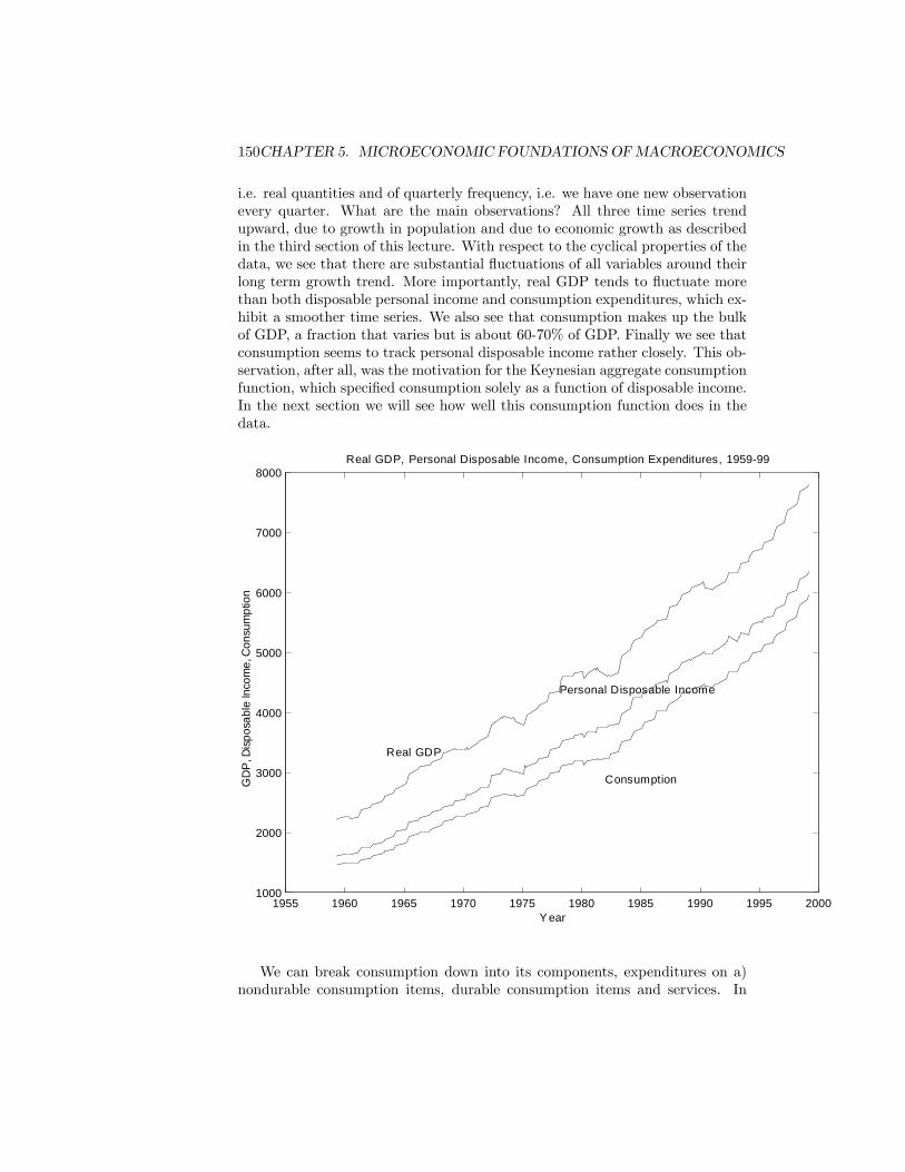
150CHAPTER 5. MICROECONOMIC FOUNDATIONS OFMACROECONOMICS

i.e. real quantities and of quarterly frequency, i.e. we have one new observationevery quarter. What are the main observations? All three time series trendupward, due to growth in population and due to economic growth as describedin the third section of this lecture. With respect to the cyclical properties of thedata, we see that there are substantial �uctuations of all variables around theirlong term growth trend. More importantly, real GDP tends to �uctuate morethan both disposable personal income and consumption expenditures, which ex-hibit a smoother time series. We also see that consumption makes up the bulkof GDP, a fraction that varies but is about 60-70% of GDP. Finally we see thatconsumption seems to track personal disposable income rather closely. This ob-servation, after all, was the motivation for the Keynesian aggregate consumptionfunction, which speci�ed consumption solely as a function of disposable income.In the next section we will see how well this consumption function does in thedata.

1955 1960 1965 1970 1975 1980 1985 1990 1995 20001000

2000

3000

4000

5000

6000

7000

8000Real GDP, Personal Disposable Income, Consumption Expenditures, 195999

Y ear

GD

P, D

ispo

sabl

e In

com

e, C

onsu

mpt

ion

Real GDP

Personal Disposable Income

Consumption

We can break consumption down into its components, expenditures on a)nondurable consumption items, durable consumption items and services. In

5.1. CONSUMPTION DEMAND 151

1997, 13.6% of all consumption expenditures were accounted for by purchases ofconsumer durables, 30.2% were due to purchases of nondurable goods and 56.2%accrued to services. Over time, the share of consumption expenditures goingto services has increased substantially, as has the share of consumer durables,whereas the share of nondurables has declined over time.When plotting these components over time (see Hall/Taylor�s Figure 10.2)

we see that, although consumer durables are the smallest item among totalconsumption expenditures, it is by far the most volatile part: purchases ofconsumer durables are particularly low during recessions and particularly highduring booms, whereas purchases of nondurables and services are relatively sta-ble over the business cycle. This fact is quite intuitive since consumer durables(cars, furniture) have investment goods character; they require a large outlay,are usually �nanced by credit and provide services for a prolonged period oftime. This investment good character of consumer durables has led economiststo think that we in fact mismeasure consumption by looking at consumptionexpenditures. When you buy a new car in 1999, the whole price for the caris counted in consumption expenditures for 1999. But the car delivers servicesfor many years (unless you bought a real lemon). Therefore from a theoreticalpoint of view the price of the car should be split up into, say, ten pieces (for tenyears of usage), and only that part of the price that corresponds to the servicesthat the car provides in the �rst year should be counted as consumption ex-penditures. This method is obviously somewhat hard to implement in practice.But once implemented it seems almost certain that expenditures on consumerdurables, measured this way, would be way less volatile than it is now with theconventional measurement technique. Hence consumption expenditures wouldbe even smoother over the business cycle that they already are.

5.1.2 The Keynesian Aggregate Consumption Function andthe Data

Now we will look in more detail at the Keynesian aggregate consumption func-tion. Remember that in its simplest form it was given as

C = a+ b(1� �)Yh= a+ bYd

where Yd is disposable income. Let us see how the function does in practice. InFigure 60 we plot total consumption expenditures as measured in the data andconsumption expenditures predicted by the aggregate consumption function for1959 to 1999. All data is in billion 1996 US dollars.We pick the parameters (a; b) in such a way as to minimize the di¤erence

between actual and predicted data, i.e. we give the aggregate consumptionfunction its best shot. Estimating the parameters that gives the best �t1 yields

1Technically, we estimate the parameters by ordinary least squares, i.e. in order to minimizethe sum of squared deviations of actual data from predicted ones.


1955 1960 1965 1970 1975 1980 1985 1990 1995 20001000

1500

2000

2500

3000

3500

4000

4500

5000

5500

6000Consumption Expenditures, Actual and Predicted, 195999

Y ear

Con

sum

ptio

n, A

ctau

l and

Pre

dict

ed

Consumption Expenditures in the Data

Consumption Expenditures Predicted by Aggregate Consumption Function

(a; b) = (�106; 0:923): The fact that the estimated a is negative is a bit bother-some, but let�s ignore this for a second. The marginal prospensity to consumeis estimated at 0:92; i.e. on average the US households spend 92 cents out ofevery additional dollar disposable income.Figure 60 may indicate that the Keynesian consumption function does rather

well. But the magnitudes on the y-axis a re substantial. Let us in Figure 61plot the deviation of actual consumption expenditures from the ones predictedby the consumption function.We see that the deviations are quite sizeable, amounting to under-or over-

estimation of actual consumption by up to 200 billion US dollar, or about 6%of total consumption expenditures in given periods. Given that consumptionexpenditures make up about two thirds of total real GDP, this under- or over-prediction may easily lead to an under -or overprediction of real GDP by 3-4%.Given that economic policy is carried out based on economic forecasts, these arehuge numbers because the prediction may easily show a healthy economy whenin fact the true data afterwards indicate that the economy was well under way


1955 1960 1965 1970 1975 1980 1985 1990 1995 2000200

150

100

50

0

50

100

150

200

250Dev iation of Consumption Expenditures f rom Predicted, 195999

Y ear

Con

sum

ptio

n D

evia

tions

into a recession. For example, in the 70�s and early 80�s realized consumptionexpenditures were quite smaller than predicted ones. According to the predic-tion �scal or monetary expansionary policy was not called for, but ex-post itturned out to be the case that the economy was or was going into a recession andan expansionary �scal or monetary policy, uncalled for based on the prediction,may have been able to prevent or at least soften the recession. The apparentmalfunction of the Keynesian aggregate consumption function, plus its weakfoundation on microeconomic principles of consumer optimization led to thedevelopment of an alternative model of consumption, the life cycle/permanentincome model of consumption.

5.1.3 The Life Cycle/Permanent Income Model of Con-sumption

In this subsection we will present and then apply a simple version of Ando-Modigliani�s life-cycle model and Friedman�s permanent income model. The


simple model we present is due to Irving Fisher (1867-1947), and the life-cycleas well as the permanent income model are relatively straightforward generaliza-tions of Fisher�s model. At the end of this section we will apply Fisher�s modelto the analysis of how a social security system a¤ects consumption demand ofhouseholds.Consider a single individual, for concreteness call this guy Freddy Krueger.

Freddy lives for two periods (you may think of the length of one period as 30years, so the model is not all that unrealistic). He cares about consumption inthe �rst period of his life, c1 and consumption in the second period of his life,c2: His utility function takes the simple form

u(c1; c2) = log(c1) + � log(c2) (5.1)

where the parameter � is between zero and one and measures Freddy�s degreeof impatience. A high � indicates that consumption in the second period of hislife is really important to Freddy, so he is patient. On the other hand, a low �makes Freddy really impatient. In the extreme case of � = 0 Freddy only caresabout his consumption in the current period, but not at all about consumptionwhen he is old.Freddy has income y1 > 0 in the �rst period of his life and y2 � 0 in the

second period of his life (we want to allow y2 = 0 in order to model that Freddyis retired in the second period of his life and therefore, absent any social securitysystem, has no income in the second period). Income is measured in units ofthe consumption good, not in terms of money. As with the Keynesian aggregateproduction function we abstract from money in this analysis. Freddy also startshis life with some initial wealth A � 0; due to bequests that he received from hisparents. Again A is measured in terms of the consumption good, not in termsof money. Freddy can save some of his income in the �rst period or some of hisinitial wealth, or he can borrow against his future income y2: We assume thatthe interest rate on both savings and on loans is equal to r; and we denote by sthe saving (borrowing if s < 0) that Freddy does. Hence his budget constraintin the �rst period of his life is

c1 + s = y1 +A (5.2)

Freddy can use his total income in period 1, y1+A either for eating today c1 orfor saving for tomorrow, s: In the second period of his life he faces the budgetconstraint

c2 = y2 + (1 + r)s (5.3)

i.e. he can eat whatever his income is and whatever he saved from the �rstperiod. The problem that Freddy faces is quite simple: given his income andwealth he has to decide how much to eat in period 1 and how much to savefor the second period of his life. The is a very standard decision problem asyou have studied left and right in microeconomics, with the only di¤erence thatthe goods that Freddy chooses are not apples and bananas, but consumptiontoday and consumption tomorrow. In micro our people usually only have one


budget constraint, so let us combine (5:2) and (5:3) to derive this one budgetconstraint, a so-called intertemporal budget constraint, because it combinesincome and consumption in both periods. Solving (5:3) for s yields

s =c2 � y21 + r

and substituting this into (5:2) yields

c1 +c2 � y21 + r

= y1 +A

orc1 +

c21 + r

= y1 +y21 + r

+A (5.4)

Let us interpret this budget constraint. We have normalized the price of theconsumption good in the �rst period to 1 (remember from micro that we couldmultiply all prices by a constant and the problem of Freddy would not change.The price of the consumption good in period 2 is 1

1+r ; which is also the relativeprice of consumption in period 2; relative to consumption in period 1: Hence thegross interest rate 1 + r is really a price: it is the relative price of consumptiongoods today to consumption goods tomorrow (note that this is a de�nition). Sothe intertemporal budget constraint says that total expenditures on consump-tion goods c1+ c2

1+r ; measured in prices of the period 1 consumption good, haveto equal total income y1 +

y21+r ; measured in units of the period 1 consumption

good, plus the initial wealth of Freddy. The sum of all labor income y1 +y21+r

is sometimes referred to as human capital. Let us by I = y1 +y21+r + A denote

Freddy�s total income, consisting of human capital and initial wealth.Now we can analyze Freddy�s consumption decision. He wants to maximize

his utility (5:1); but is constrained by the intertemporal budget constraint (5:4):To let us solve

maxc1;c2

flog(c1) + � log(c2)g

s:t: c1 +c21 + r

= I

One option is to use the Lagrangian method, which you should have seen inMicroeconomics, and you should try it out for yourself. The second option is tosubstitute into the objective function for c1 to get

maxc2

�log

�I � c2

1 + r

�+ � log(c2)

�This is an unconstrained maximization problem. Let us take �rst order condi-tions with respect to c2

� 11+r

I � c21+r

+�

c2= 0


or

c21 + r

= �

�I � c2

1 + r

�c2 = � ((1 + r)I � c2)

(1 + �)c2 = �(1 + r)I

c2 =�

1 + �(1 + r)I (5.5)

=�

1 + �((1 + r)(y1 +A) + y2) (5.6)

Since c1 = I � c21+r we �nd

c1 = I � c21 + r

= I � �

1 + �I

=I

1 + �

=1

1 + �

�y1 +

y21 + r

+A

�(5.7)

Since saving s equals y1 +A� c1 we �nd

s =�

1 + �(y1 +A)�

y2(1 + �)(1 + r)

which may be positive or negative, depending on how high �rst period incomeand initial wealth is compared to second period income. So Freddy�s optimalconsumption choice today is quite simple: eat a fraction 1

1+� of total lifetimeincome I today and save the rest for the second period of your life.So on what variables does current consumption depend on? According to our

model it is income today, income next period, initial wealth A and the interestrate r: All those variables, apart from income today, did the simple Keynesianaggregate consumption function ignore. But even the simplest model that hasconsumers deciding optimally on their consumption predicts that future income,the intertemporal price of consumption (the interest rate) and initial wealthholdings should enter the consumption function. More complex models basedon consumer optimization add even more variables.For now let us stick with our simple model. As in microeconomics we can

analyze the decision problem of Freddy graphically, using budget lines and in-di¤erence curves. First we plot the budget line (5:4): This is the combinationof all (c1; c2) Freddy can a¤ord. We draw c1 on the x-axis and c2 on the y-axis.Looking at the left hand side of (5:4) we realize that the budget line is in facta straight line. Now let us �nd two points on the line. Suppose c2; i.e. Freddydoes not eat in the second period. Then he can a¤ord c1 = y1 +A+

y21+r is the


�rst period, so one point on the budget line is (ca1 ; ca2) = (y1+A+

y21+r ; 0): Now

suppose c1: Then Freddy can a¤ord to eat c2 = (1+r)(y1+A)+y2 in the secondperiod, so a second point on the budget line is (cb1; c

b2) = (0; (1+r)(y1+A)+y2):

Connecting these two points with a straight line yields the entire budget line.We can also compute the slope of the budget line as

slope =cb2 � ca2cb1 � ca1

=(1 + r)(y1 +A) + y2

��y1 +A+

y21+r

�= �(1 + r)

Hence the budget line is downward sloping with slope (1 + r): Now let�s tryto remember so microeconomics. The budget line just tells us what Freddycan a¤ord. The utility function (5:1) tells us how Freddy values consumptiontoday and consumption tomorrow. Remember that an indi¤erence curve is acollection of bundles (c1; c2) that yield the same utility, i.e. between whichFreddy is indi¤erent. Let us �x a particular level of utility, say u (which is justa number). Then an indi¤erence curve consists of all (c1; c2) such that

u = log(c1) + � log(c2)

Solving for c2 yields

log(c2) =u� log(c1)

�

c2 = eu�log(c1)

� = eu� c

�1�

1

Hence as c1 becomes bigger and bigger, c2 approaches 0: As c1 approaches 0; c2becomes bigger and bigger. See Figure 62 for a typical shape of an indi¤erencecurve. The slope of the indi¤erence curve is given as

dc2dc1

=�1�eu� c

�1� �11

=�1�c1

eu� c

�1�

1

=�c2�c1

Incidently this slope equals the (negative of the) marginal rate of substitution(as always)

MRS =uc1(c1; c2)

uc2(c1; c2)=c2�c1

where uci indicates the partial derivative of u with respect to ci: From the �gurewe note that Freddy should pick his consumption such that the indi¤erence curve


c* y +A y +A+y /(1+r) c1 1 1 2 1

Saving s

Indifference curvelog(c )+βlog(c )=constant

1 2

Budget line

Slope

1+r

Slope c / βc2 1

c2

(1+r)(y +A)+y1 2

c*2

y2

is tangent to the budget line. This means that at the optimal consumption choicethe slope of the indi¤erence curve and the budget line are equal or

uc1(c1; c2)

uc2(c1; c2)= 1 + r

uc1(c1; c2) = (1 + r)uc2(c1; c2) (5.8)

This equation has a nice interpretation. At the optimal consumption choice thecost, in terms of utility, os saving one more unit should be equal to the bene�tof saving one more unit (if not, Freddy should either save more or less). Butthe cost of saving one more unit, and hence one unit lower consumption in the�rst period, in terms of utility equals uc1(c1; c2): Saving one more unit yields(1 + r) more units of consumption tomorrow. In terms of utility, this is worth(1+r)uc2(c1; c2): Equality of cost and bene�t implies (5:8): Using the particularfrom of the utility function yields as the condition for an optimal consumptionchoice

c2�c1

= 1 + r


This, together with the intertemporal budget constraint (5:4) can be solvedfor the optimal consumption choices, which obviously gives the same result asbefore.

Income and Interest Changes

Now we can investigate how changes in today�s income y1; next period�s incomey2 and initial wealth A change the optimal consumption choice. From (5:7) and(5:5) we see that both c1 and c2 increase with increases in either y1; y2 or A:In contrast to the Keynesian consumption function, an increase in tomorrow�sincome will increase today�s consumption as well as tomorrow�s consumption.The marginal prospensity to consume out of today�s income or initial wealth is

dc1dA

=dc1dy1

=1

1 + �> 0

and the marginal prospensity to consume today out of tomorrows income equals

dc1dy2

=1

(1 + �)(1 + r)> 0

We see this e¤ect graphically in Figure 63. The e¤ect of increases in both c1and c2 in reaction to increases in y1; y2 or A is called an income e¤ect.More complicated are changes in the interest rate, since this will entail in-

come e¤ects and substitution e¤ects. A substitution e¤ect comes about since thegross interest rate 1+ r is the relative price of consumption in period 1; relativeto consumption in period 2: So as the interest changes, not only does incomechange (because y2

1+r changes), but also the relative price of consumption goodsin the two periods.Let us analyze an increase in the interest rate from r to r0 and let us start

graphically. What happens to the curves in Figure 62 as the interest rate in-creases? The indi¤erence curves do not change, as they do not involve theinterest rate. But the budget line changes. Since we assume that the interestrate increases, the budget line gets steeper. And it is straightforward to �nda point on the budget line that is a¤ordable with old and new interest rate.Suppose Freddy eats all his �rst period income and wealth in the �rst period,c1 = y1 + A and all his income in the second period c2 = y2; in other words,he doesn�t save or borrow. This consumption pro�le is a¤ordable no matterwhat the interest rate (as the interest rate does not a¤ect Freddy as he neitherborrows nor saves). This consumption pro�le is sometimes called the autarkicconsumption pro�le, as Freddy needs no markets to implement it: he just eatswhatever he has in each period. Hence the budget line tilts around the autarkypoint and gets steeper, as shown in Figure 64.Consumption in period 2 increases and consumption in period 1 decreases.

Saving increases. This is also apparent from equations (5:7) and (5:5). Whatis the reason? There are two e¤ects from an increase in the interest rate. Firstthere is an income e¤ect: if Freddy is a saver (as we assume in the picture)


c* c*’ y +A c1 1 1 1

Budget lines

Slopes

1+r

Slope c / βc2 1

c2

(1+r)(y +A)+y1 2

c*2

y2

’

c*’2

then a higher interest rate, for given savings, increases his income in the secondperiod. The in�uence of this e¤ect on both c1 and c2 is positive and is called theincome e¤ect. Also, an increase in the interest rate makes consumption todaymore expensive compared to consumption tomorrow, so individuals substitutesubstitute consumption today with consumption tomorrow. This is the substi-tution e¤ect: it is negative for c1 and positive for c2: Hence c2 unambiguouslyincreases; for c1 it depends on the size of the income and the substitution e¤ect.For the particular utility function we chose and the assumptions on income wemade c1 decreases and saving increases. Note that if the consumer is a borrowerthen the income e¤ect is negative rather than positive: a higher interest rateincreases the interest payments on his loan. The substitution e¤ect works asbefore. Hence for a borrower we can conclude that consumption in the �rstperiod declines in a response to an increase in the interest rate (both incomeand substitution e¤ects are negative). Consumption in the second period mayincrease or decline, depending on whether the positive substitution e¤ect isstronger or weaker than the negative income e¤ect (again for our assumptions


c*’ c* y +A c1 1 1 1

Budget lines

Slope

1+r

Slope c / βc2 1

c*2

y2

c*’2

the substitution e¤ect is stronger).So far we assumed that Freddy could borrow freely at interest rate r: But

we all (at least some of us) know that sometimes we would like to take out aloan from a bank but are denied it. Let us analyze how the presence of so-calledborrowing constraints a¤ect the consumption choice. So let us assume thatFreddy cannot borrow, so he is constrained by s � 0: Obviously if Freddy is asaver anyway, nothing changes for him since the constraint on borrowing is notbinding. The situation is di¤erent if, without the borrowing constraint, Freddywould be a borrower. Now with the borrowing constraint, the best he can do isset c1 = y1 + A; c2 = y2: He would like to have even bigger c1; but since he isborrowing constrained he can�t bring any of his second period income forward bytaking out a loan. Note that in this situation Freddy�s �rst period consumptiondoes not depend on second period income or the interest rate. In particular, ify2 goes up, c1 remains unchanged if Freddy is borrowing-constrained. This canbe seen from Figure 65.The budget line with the presence of borrowing constraints has a kink at


c = y +A c1 1 1

Budget line

Slope

1+r

Slope c / βc2 1

c2

c = y2 2

Indifference

Curves

c’ = y’2 2

(y1 + A; y2): For c1 < y1 + A we have the usual budget constraint, as heres > 0 and the borrowing constraint is not binding. But with the borrowingconstraint Freddy cannot a¤ord any consumption c1 > y1 + A; so the budgetconstraint has a vertical segment at y1 + A; because regardless of what c2;the most Freddy can a¤ord in period 1 is y1 + A: If Freddy was a borrowerwithout the borrowing constraint, then his optimal consumption is at the kink.And with an increase of second period income y2; Freddy just increases secondperiod consumption, with �rst period consumption unchanged. Also not that(as long as the borrowing constraint remains binding, Freddy will consume everycent of an income increase in the �rst period immediately in the �rst period,i.e. his marginal prospensity to consume out of current income is 1 if Freddy isborrowing-constrained.Hence with borrowing constraints the consumption function of Freddy looks

much more Keynesian: consumption only depends on current income and isindependent of the interest rate and future income. Since in the overall economythere are individuals that face borrowing constraints and others who do not, we


can expect the aggregate consumption function to depend heavily on currentincome, but also on future income and the interest rate. We saw in the �rstsection how the Keynesian aggregate consumption function fared with respectto the data. A huge amount of empirical work has been done to test moreelaborate versions of the simple Fisher model. We come back to this later.

Borrowing constraints may be one explanation of why the Japanese savingrate is higher than the US saving rate. Individuals that are borrowing con-strained consume less (and save more) than they otherwise would, without theborrowing constraint. The biggest expense, particularly for young families isusually the purchase of the �rst home. In the US, a down payment of about10% on a house is quite common, the rest is borrowed. In Japan down pay-ments of 40% or higher are common, hence households are much more borrow-ing constrained in Japan than in the US, at least with respect of this particulartransaction. Hence Japanese have to save more in advance to �nance home pur-chases, which explains part of their higher saving rate. Note that, although alot of economists argue that a high saving rate is good for growth, the particularfeature of the Japanese economy that brings the higher saving rate about (highdown payments) is usually not regarded as desirable.

Social Security in the Life-cycle model

Now we use the model to analyze a policy issue that has drawn large attention inthe public debate. The personal saving rate -the fraction of disposable incomethat private households save- has declined from about 7-10% in the 60�s and70�s to 2.1% in 1997. Since saving provides the funds for investment a lowersaving rate, so a lot of people argue, harms growth be reducing investment.2

Some economists argue that the expansion of the social security system hasled to a decline in personal saving. We want to analyze this claim using oursimple model. We look at a pay-as-you go social security system, in which thecurrently working generation pays payroll taxes, whose proceeds are used to paythe pensions of the currently retired generation. The key is that current taxes arepaid out immediately, and not invested. We make the following simpli�cationsto our model. We interpret the second period of a person�s life as his retirement,so in the absence of social security he has no income apart from his savings, i.e.y2 = 0: For simplicity we also assume A = 0: Without social security3 we have

2This argument obviously ignores increased government saving in the US and the increasedin�ow of foreign funds into the US.

3Conceptually a fully funded system is as if everybody saves for him- or herself. We abstractfrom uncertainty about the length of life and hence from insurance aspects of a socail securitysystem.


from before

c1 =y11 + �

c2 =�(1 + r)y11 + �

s =�y11 + �

Now suppose we introduce a pay as-you-go social security system. As a con-sequence in the �rst period of his life Freddy has to pay payroll taxes. Let usassume that the tax rate on labor income is � ; so Freddy�s after tax wage is(1� �)y1: Note that currently the payroll tax for social security is 15:3%; paidhalf by the employer and half by the employee. This includes contributionsto medicare and disability insurance. In the second period of his life he nowreceives social security payments SS: Let us assume that the population growsat rate n; so when Freddy is old there are (1 + n) as many young guys aroundcompared when he was young. Also assume that pre-tax-income grows at rateg; so the income of the young people, when Freddy is old, equals (1 + g)y1 theincome that Freddy had when he was young. Finally assume that the social se-curity system balances its budget, so that total social security payments equaltotal payroll taxes. This implies that

SS = (1 + g)(1 + n)�y1

Freddy bene�ts from the fact that population and wages grow over time sincewhen he is old there are more people around to pay his pension from higherwages of theirs. Now Freddy has the budget constraints

c1 + s = (1� �)y1c2 = (1 + r)s+ SS

Again we can write this as a single intertemporal budget constraint

c1 +c21 + r

= (1� �)y1 +SS

1 + r= I (5.9)

Maximizing (5:1) subject to (5:9) yields, by the same logic as before

c1 =I

1 + �

c2 =�

1 + �(1 + r)I


Now we use the fact that SS = (1 + g)(1 + n)�y1 since the budget of the socialsecurity system has to be balanced. Therefore

I = (1� �)y1 +SS

1 + r

= (1� �)y1 +(1 + g)(1 + n)�y1

1 + r

= y1 ��1� (1 + g)(1 + n)

1 + r

��y1

= ~y1

where we de�ned ~y1 to be the mess on the right hand side. Hence

c1 =~y1

1 + �

c2 =�

1 + �(1 + r)~y1

Comparing this with the result from before we see that consumption in bothperiods is higher with social security than without if and only if ~y1 > y1; i.e. ifand only if (1+g)(1+n)1+r > 1: Hence people are better o¤ with social security if

(1 + g)(1 + n) > 1 + r

This condition makes perfect sense. If people save by themselves for their re-tirement, the return on their savings equals 1 + r: If they save via a socialsecurity system ( are forced to do so), their return to this forced saving consistsof (1 + n)(1 + g) (more people with higher wages pay for the old guys). Thisresult makes clear why a pay-as-you-go social security system may make sensein some countries (those with high population and wage growth), but not inothers, and that it may have made sense in the US in the 60�s and 70�s, but notin the 90�s. Just some numbers: the current population growth rate is aboutn = 1%; growth of wages and salaries is about g = 2%; and the average returnon the stock market for the last 100 years is about r = 7% (and obviously muchhigher recently). This is the basis for many economists to call for a reform of thesocial security system, most prominently Martin Feldstein, chief of the NationalBureau of Economic Research, the most important economic think tank in theUS. There is an intense debate over how one could privatize the social securitysystem, i.e. create individual retirement funds so that basically each individualwould save for her own retirement, with return 1+r > (1+g)(1+n): The biggestproblem is one missing generation: at the introduction of the system in the 30�sthere was one old generation that received social security but never paid taxesfor it. Now we face the dilemma: if we abolish the pay-as-you go system, eitherthe currently young pay double, for the currently old and for themselves, or wejust default on the promises for the old. Both alternatives seem to be di¢ cultto implement politically and problematically from an ethical point of view. Thegovernment could pay out the old by increasing government debt, but this has


to be �nanced by higher taxes in the future, i.e. by currently young and futuregenerations. Hence this is problematic, too. The issue is very much open, andsince I did research on this issue in my thesis I am happy to talk to whoever isinterested in more details.But back to the original question: what does pay-as-you go social security

do to saving? Without social security saving was given as

s =�y11 + �

with social security it is given by

s =�(1� �)y1 � SS

1+r

1 + �

and obviously private saving falls. Note that the social security system as partof the government does not save, it pays all the tax receipts out immediatelyas pensions. So saving unambiguously goes down with social security. To theextent that this harms investment, capital accumulation and growth the pay-as-you-go social security system may have substantial negative long-run e¤ects,over and above the e¤ects due to its lower return as compared to private savingfor retirement.4

This analysis shows that, although or model is very simple, it is quite pow-erful in addressing an array of interesting policy questions. Now we turn to adescription of more involved models of consumption choice that build on thissimple model.

Extensions of the Basic Model

In the mid-50�s Franco Modigliani, jointly with Albert Ando and Richard Brum-berg developed the life-cycle hypothesis of consumption. The basic insight ofthe simple model above builds the corner stone of the life-cycle hypothesis: in-dividuals want a rather smooth consumption pro�le over their life, but theirlabor income varies substantially over their lifetime, starting out low, increasingup until about the 50�th year of a person�s life and then slightly declining until65, with no labor income after 65. The life-cycle hypothesis then states that bysaving (and borrowing) individuals achieve it that they turn a very nonsmoothlabor income pro�le into a very smooth consumption pro�le. Therefore the lifecycle hypothesis predicts that current consumption (as well as future consump-tion) depends on total lifetime income and given initial wealth, as in the simplemodel. The life-cycle model stresses the importance of saving: in particular sav-ing should follow a very pronounced life-cycle pattern with little saving (or evenborrowing) in the early periods of an economic life (which usually is assumedto begin around 16-20), signi�cant saving in the high earning years from 35-50

4 In this simple model there is really no bene�cial role for a pay-as-you-go system. Thischanges as one introduces mortality risk or income distribution considerations into the model.


and dissaving in retirement years as the accumulated wealth is used to provideconsumption in old age.The life-cycle version of the model seems to fare quite well when confronted

with data from the Consumer Expenditure Survey or other data sources thatrecord individual households incomes and consumption expenditures. One em-pirical fact that puzzles life-cyclers is the observation that older, retired house-hold do not dissave to the extent predicted by the theory. There are severalexplanation for this puzzle. One is that, contrary to the assumptions of thetheory, individuals are altruistic and want to leave bequests to their children.A di¤erent explanation is that it is highly uncertain how long one lives andwhether one stays healthy. If older households are extremely risk-averse andfear the possibility of living very long and hence not having saved enough -orif they fear the risk of getting sick and the resulting huge medical bills, then itmay be rational to keep almost all savings intact to be prepared for this veryunlikely, but very deeply feared event.Milton Friedman�s permanent income hypothesis is also an immediate ex-

tension of the basic model discussed above. Instead of stressing the life-cycleaspect of consumption and saving Friedman focussed on the fact that futurelabor income is uncertain to a certain degree. He posited that the income ofan individual household, y consists of a permanent part, yp and a transitorypart yt; i.e. y = yp + yt: One may think of the permanent part as expectedaverage future income and of the temporary part as the random �uctuationsaround this average income. Examples may help: your usual salary makes upthe largest fraction of your permanent income. A win in the lottery is thetypical component of transitory income, or a particularly good summer for anice-cream vendor, something that increases (or decreases) your income, but isnot a permanent event. Friedman observed correctly that individuals wouldreact quite di¤erently to an increase in permanent and an increase in transitoryincome. Suppose you start a new, permanent job that doubles your salary upinto the inde�nite future. By how much would you increase your consumptionexpenditures? Now suppose you win $1,000 in the lottery, and the chances ofthat happening again are very small. By how much would you increase yourconsumption expenditures? Friedman claimed that an increase in the perma-nent component of income would bring about an (almost) equal response inconsumption, whereas individuals would smooth out transitory income shocksover time: you take the 1,000 bucks and spend $50 to see Stanford beat Berkeleyand the rest you put in your saving account for future usage. It then follows thatindividual consumption is almost entirely determined by permanent income, i.e.by the average income you think you will make for the rest of your life. Formally

c = �yp

where � is a parameter close to 1: Again we have the insight that consumptiontoday depends on future income (expectations) rather than on current income,which may be unusually high (because of a positive transitory shock) or unusu-ally low (because of a negative transitory shock).


A large empirical literature has investigated the life-cycle and permanentincome theories of consumption demand.5 Although the book is not closedyet, it appears that the data seem quite favorable to these theories. Becauseof this and because of the fact that these theories have sound foundations inmicroeconomics they are the leading theories in current research on consumptionand saving behavior.

5.2 Investment Demand

Before turning to the theoretical analysis of investment demand let us havea look at the data. Although investment is a much smaller fraction of totalGDP than consumption, the analysis of investment demand is is crucial for theanalysis of business cycles as investment demand is much more volatile thanconsumption demand and GDP. Remember that we could divide total grossinvestment into three categories:

1. Residential Fixed investment: this is the spending of private householdson the construction of new houses and apartments

2. Nonresidential Fixed Investment; this is the spending of �rms on newplants and equipment

3. Inventory investment: this is the change of the value of inventories heldby businesses. Inventory investment can be positive (inventories increase)or negative (inventories decline).

5.2.1 Facts about Investment

In Figure 66 we plot real GDP and real gross investment over tiem for the US.Note that the scale on the two sides of the graph is di¤erent. The scale on theleft side is the relevant scale for real GDP, whereas the scale on the right side isrelevant scale for gross investment. This techinque of plotting the time series ischosen to enable better comparison between the �uctuations of GDP and grossinvestment. Comparing the two plots we observe the following features

1. Gross Investment is about 15% of real GDP on average. This fraction, theso called investment-output ratio �uctuates over the business cycle, goingdown in recessions and up in booms, but is fairly constant in the long run.

2. Gross Investment �uctuates much more severely than real GDP, withmore pronounced declines in recessions and more pronounced increasesin booms. In this sense gross investment is that part of GDP that ismostly responsible for the business cycle.

5An excellent book that discusses the theories as well as their empirical tests is AngusDeaton�s (1992) �Understanding Consumption�.

5.2. INVESTMENT DEMAND 169

1955 1960 1965 1970 1975 1980 1985 1990 1995 20000

5000

10000Real GDP, Gross Inv estment, 195999

Y ear

GD

P a

nd G

ross

Inve

stm

ent

1955 1960 1965 1970 1975 1980 1985 1990 1995 20000

1000

2000

Real GDP

Gross Inv estment

Now we break down gross investment into its components, residential �xedinvestment, nonresidential �xed investment and changes in business inventories.In Figure 67 we plot gross investment and its �rst two components over time,leaving for Figure 68 the plot changes in inventories. From Figure 67 we seethat over time nonresidental �xed investment (plant and equipment purchasesof �rms) have become relatively more important compared to residential �xedinvestment. Whereas in 1959 made up about 50% of total gross investment, in1999 nonresidential �xed investment made up around 74% of total gross invest-ment and residential �xed investment around 23% (the rest going to changesin inventories). It also appears from this �gure that both residential as well asnonresidential �xed investment �uctuate less over time as total gross investment.The last fact obviously implies that the remaining part of investment, namely

changes in business inventories, has to �ucutate a lot over the business cycle.This conjecture is veri�ed in Figure 68, where we plot total investment andinventory investment. Again notice that we have used di¤erent cales for bothvariabl;es to enable easier comparison.


1955 1960 1965 1970 1975 1980 1985 1990 1995 20000

200

400

600

800

1000

1200

1400

1600

1800Real Gross Inv estment and Components, 195999

Y ear

Inve

stm

ent a

nd C

ompo

nent

s

Gross Inv estment

Residential Fixed Inv estment

Nonresidential Fixed Inv estment

In paricular the scale on the left side is for total investment, whereas the scaleon the right side is for inventory investment. We see that inventory investment�ucuates much more than total investment, or, for that matter, much strongerthan any ohter component of real GDP. Hence, although inventory investmentmakes up only about 1% of GDP, it is a strong contibutor to business cyclesand inventory investment of �rms is heavily studied by both theoretical as wellas empirical economists trying to explain the business cyle. Also note thatduring recessions inventory investment typically becomes (or at least gets closeto) negative: during recessions �rms tend not to produce for inventory.

After this little tour overviewing the basic facts with respect to investmentdata let us now look at soem theory trying to explain the investment behaviorof �rms.


1955 1960 1965 1970 1975 1980 1985 1990 1995 20000

1000

2000Gross Inv estment and Change in Inv entories, 195999

Y ear

Gro

ss In

vest

men

t, C

hang

e in

Inve

ntor

ies

1955 1960 1965 1970 1975 1980 1985 1990 1995 2000100

0

100

Gross Inv estment

Change in Inv entories

5.2.2 The Theory of Investment

Nonresidential Fixed Investment Demand

To start our study of investment demand of a single we proceed in two steps. We�rst assume that our �rm rents all capital that it uses in the production processfrom other �rms that are in the business of equipment and plant renting forindustrial purposes. Although in reality most equipment and plants used are infact owned by the �rms who use it, this assumption will turn out not to matter.Let the rental price for one unit of the capital good be denoted by rk and thewage for one worker be denoted by w: We normalize the price of the outputgood to 1, so rk and w are the real rental price of capital and the real wage,respectively. Let us assume that the �rm can produce output Y according tothe following production function

Y = K�L1��


where K is the amount of capital rented and L is the number of workers hired.To determine the �rm�s demand for rented capital we have to solve the �rm�spro�t maximization problem

maxK;L

K�L1�� rkK � wL

The �rst part of the above equation is the revenue the �rm takes in (rememberthat we normalized the price of the �nal output good to 1), and the second andthird part are the total costs for renting capital and hiring workers, respectively.Taking the �rst order condition with respect to capital yields

rk = �K��1L1�� =

�KaL1��

K=�Y

K

solving this for K gives the optimal demand for capital to be rented, K; as

K =�Y

rk(5.10)

Hence, if the �rm decides to produce output Y and faces a rental price of capitalrk; then the optimal amount of capital to rent out is given by K = �Y

rk: This

is the standard pro�t maximization condition from micro: the �rm should hireinputs, in particular capital, to the point where the additional cost for oneunit rented, rk, equals the additional bene�t, the marginal product of capital,�K��1L1��: This gives a demand curve for capital that is increasing in thedesired amount of output produced, Y; and decreasing in the rental rate ofcapital rk:In Figure 69 we plot the demand for rented capital as a function of the rental

rate of capital. As good (actually bad!) tradition in microeconomics we plotthe price (the rental rate rk) on the y-axis and the quantity of rental capitaldemanded on the x-axis. In this graph we hold the desired level of outputconstant. As indicated in (5:10) the quantity demanded of capital decreaseswith the rental rate rk: The optimal quantity demanded at the price rk is givenby K�; because at this level of the capital stock the marginal cost from rentingan additional unit, rk is equal to the marginal product �Y

K ; for a given level ofoutput Y:Figure 70 shows what happens to the demand curve for rented capital if the

planned level of output increases. Again as (5:10) shows an increase in Y; for�xed rk increases K: But this is true for every rk; indicating that the entiredemand curve shifts to the right. If the rental price of capital doesn�t change,the new optimal choice of capital is now K 0� > K�; i.e. the �rm reacts to higherdesired output by demanding more rented capital (and more workers).So far we have ignored the fact how the rental price of capital is determined.

So let us consider the hypothetical problem of a �rm engaged in the business ofrenting out capital, i.e. equipment and plants. For concreteness let us considerthe choice of such a �rm buying a particular piece of equipment. Let pk denotethe relative price of equipment (relative to the price of the �nal output good),


Marginal Cost ofCapital

Marginal Product ofCapital

rk

K* Demand for Rented Capital (K)

Rental price

of capital

r denote the real interest rate and � the depreciation rate. What are the costsand what are the revenues from purchasing this machine and renting it out inthe current period? The revenues in the current period equal rk: The costs arecomposed of two parts. The �rm has to �nance the purchase by borrowing themoney to purchase the machine. The interest on the loan is a cost, equal torpk: Furthermore a part � of the machine wears out in the production process.The loss of value due to this wearing out amounts to �pk in the current period.Since there is free entry into the business of renting out capital pro�ts are bitdown to zero and therefore it must be the case that

rk = (r + �)pk

So the rental price of capital equals the interest rate plus the rate of depreci-ation, times the relative price of investment goods to consumption goods, pk:This relative price in turn depends on the technology that speci�es how muchof the �nal output good is needed to produce one unit of the investment good.In a lot of macro models we assume that output can be used both for consump-


Marginal Cost ofCapital

Marginal Product ofCapital

rk

K* K’* Demand for Rented Capital (K)

Y

Rental price

of capital

tion and investment on a 1-1 basis (remember the Solow model) in which casepk = 1: These types of models are called one-sector models as there is only oneproduction sector that produces both consumption and investment goods. Wewill focus on these types of models as they are most tractable. We then havea direct relation between the rental rate of capital and the real interest rate ofthe form rk = r + � and the demand for rented capital depends negatively onthe real interest rate.The remaining step is to relate the desired rented capital stock and invest-

ment demand. Consider a hypothetical �rm that does two things: it purchasescapital goods and rents it to itself and it produces output. Suppose this �rmenters the period with capital stock K�1: The demand of the �rm for rentedcapital services is given by

K =�Y

r + �

and the investment demand of the consolidated �rm (taking the output produc-


ing and the capital renting division together) equals

I = K � (1� �)K�1

=�Y

r + �� (1� �)K�1

This is the investment demand for a single �rm. It depends positively on theoutput that this �rm produces and negatively on the real interest rate. Sum-ming over all �rms in the economy we get the total demand for nonresidential�xed investment. As for the individual �rm the aggregate nonresidential �xedinvestment demand depends positively on the level of output in the economyand negatively on the real interest rate. Hence our more careful study of invest-ment demand has revealed that our simple investment function from above wascorrect in that the real interest rate entered negatively, but it disregarded thein�uence of current output Y on aggregate investment demand.

Residential Fixed Investment Demand

For residential �xed investment we can carry out a similar analysis. We startby assuming that the demand for housing H decreases as the rent rh increases.The relation between rh and H is identical to the relation between rk and K;just relabel the axes in Figure 69. Also by the same reasoning the price for anew apartment building ph; the depreciation rate for buildings �h and the realinterest rate r are related by

rh = (r + �h)ph

and the investment demand for residential �xed investment is, as above, a nega-tive function of the real interest rate. To the extent that the demand for housingdepends positively on income (equal to spending), the demand for residential�xed investment also depends positively on Y; hence has the same qualitativefeatures as nonresidential �xed investment demand.

Inventory Investment Demand

A small fraction of total investment demand (usually not more than 1% of GDP)comes from changes in inventories. Although the change in inventories may besmall (but very volatile over the business cycle), the total inventories held inthe entire economy are quite substantial. Hall and Taylor report that in 1995inventories amounted to about 17% of GDP. Note that holding inventories isnot costless for �rms. Suppose the production of the goods in inventories hasbeen �nanced by credit, then if the price all for the goods held in the inventoryis pk; the current period cost of holding the inventory is (r + �i) pk; i.e. equalsto the cost of capital bound in the inventory as well as the depreciation of thegoods being held in inventories. Note that �i may be small (in the case of highlydurable goods), very large (in the case of, say, vegetables) or even negative (forgoods that appreciate, like wine).


What are the bene�ts of inventories. One �rst observation is that inventoriesmay be required in the production process. Whiskey is an example. Whiskeyhas to be stored for a while before it reaches its best quality. So putting Whiskeyinto inventory for some time is a requirement of the production process. Oil isa second example. Unavoidably large fractions of all oil produced and sold isin transit in pipelines, in involuntary inventory, so to speak. More traditionalexamples includes inventories in the manufacturing industry, where certain in-termediate goods are stored in inventories before being used in the productionprocess. Just-in-time production techniques have sharply reduced inventories ofthis kind in the last 15 years or so.Secondly inventories serve a bu¤er function against unexpected �uctuations

of demand. Final goods are put into inventory so that they are available upondemand. The bene�t from having an inventory is to be able to serve demandimmediately and hence to avoid losing the customer to a competing supplier.Of course these bene�ts have to be balanced against the cost of holding theinventory, as discussed above.Empirically changes in inventory investment is a strongly procyclical vari-

able, it tends to increase with overall production and tends to decline withoverall production. A higher level of production requires more goods �in thepipeline� and in intermediate inventories. Booms are also times where �rmsexpect high demand that they want to bu¤er with high inventory of �nal goods.Occasionally �rms are caught by surprise in that their sales expectations arenot met and inventories are accumulated involuntarily. This explains the fewoccasions where we observed a strong positive change in inventory investmentand a recession (as in 1974). For more details see Hall/Taylor�s Figure 11.8 onp. 321.To summarize, our analysis of investment demand has recon�rmed our pre-

vious assumption that aggregate investment demand depends negatively on thereal interest rate. It has added the insight that investment demand should de-pend positively on the level of output, a fact that was ignored in the traditionalaggregate investment function and the IS-LM analysis based on it.

Chapter 6

Trade, Exchange Rates &International FinancialMarkets

Foreign trade is a central policy issue. The high and increasing US trade de�citis of immediate concern to policy makers and there is a lot of controversy how toreduce it. Since the trade de�cit is closely related to the exchange rate (the valueof the dollar compared to other currencies), some economists believe that, inorder to control the trade de�cit, the exchange rate has to be controlled. Hencethe discussion of the trade de�cit leads us directly to the discussion about �xedvs. �exible exchange rates and the international �nancial system.

6.1 Terms of Trade, the Nominal and the RealExchange Rate

In order to organize our thoughts we need a few de�nitions

De�nition 8 The trade balance is total value of exports minus the total valueof imports of the US with all its trading partners. In symbols

TB = X �M

Hence the trade balance is an important component of total spending in theeconomy. For the US the trade balance has been negative for the last 20 years,as can be seen from Figure 71. For 1997 the trade balance for the US is around-100 billion dollar, i.e. the US had a trade de�cit of about 1.2% of GDP. For1999 the trade de�cit is projected to reach about 3.5% of GDP

De�nition 9 The current account balance equals the trade balance plus netunilateral transfers

CAB = TB +NUT

177

178CHAPTER 6. TRADE, EXCHANGE RATES & INTERNATIONAL FINANCIALMARKETS

1970 1975 1980 1985 1990 1995 2000400

350

300

250

200

150

100

50

0

Trade Balance for the US 19672001 (in Constant Prices)

Year

Trad

e Ba

lanc

e

The main ingredient of net unilateral transfers are interest payments topeople living in the US holding government bonds of foreign countries, netof interest payments on US government debt to foreigners. For the US netunilateral transfers are slightly negative, about 0.3% of GDP in 1997. For somehighly indebted countries, in particular in South America and South East Asia,net unilateral transfers can be signi�cantly negative, amounting to about 5% to10% of GDP. Remember again what a negative current account balance means.For this we have to understand another de�nition

De�nition 10 The Capital Account Balance is the change in the net wealthposition of the US during a year.

It follows from basic rules of accounting that the current account balancealways equals the capital account balance. A negative current account balancemeans a negative capital account balance, and this means that the net wealthposition of the US, the amount that the US (the government and its citizens)is owed, net of what it owes, decreases. The persistent current account de�citsof the US have led to the fact that in the early 80�s the US, traditionally a

6.1. TERMS OF TRADE, THE NOMINAL AND THE REAL EXCHANGE RATE179

net creditor (having a positive net wealth position with the rest of the world)turned into a net debtor (having a negative net wealth position with the rest ofthe world). This tendency seems to continue without sign of reversal.An important determinant of the trade balance is the relative price of US

goods to foreign goods. If US goods are expensive relative to Japanese goods,a lot of Japanese goods will be imported by the US and few US goods will beexported to Japan. Therefore, in order to understand the trade balance we haveto understand exchange rates

De�nition 11 The nominal exchange rate e is the relative price of twocurrencies.

For example, if the exchange rate between the dollar and the euro is 0:98;then one has to pay 0:98 euros to purchase one dollar, or reversely, one has topay 1:02 dollar to buy one euro. These days most exchanged rates are �exible:they are determined on international capital markets beyond the direct controlof national governments (obviously monetary and �scal policy will in�uence theexchange rate of the domestic currency, but under a �exible exchange rate regimethe government does not directly �x the exchange rate). The opposite is a regimeof �xed (sometimes called pegged) exchange rates: via international agreementsexchange rates between certain countries are �xed. Before the collapse of theBreton Woods system in 1973, for example, the exchange rates of the westernindustrialized countries were pegged. These days, for example, the Argentinianpeso is pegged to the dollar: the exchange rate between the dollar and the pesois 1 and the Argentinian government committed to defend this exchange rate.1

De�nition 12 The real exchange rate " is the relative price of goods in twocountries.

As it turns out it is the real exchange rate that is the key for net exports,i.e. the trade balance. To see this, consider the following example. Think of agood that is produced in many countries, say cars. Suppose a Ford Escort costs$12,000 and a similar car, a Honda Civic costs 1,890,000 yen. How expensive isa Ford relative to a Honda, i.e. how many Fords do we have to exchange for oneHonda Civic. This is exactly what the real exchange rate tells us (if all that istraded between the US and Japan were Ford Escorts and Honda Civics). Nowwe have to bring in the nominal exchange rate, since the price of the Japanesecar is measured in yen, the price of US cars in dollars. Suppose the exchangerate between the yen and the dollar is 105; i.e. one needs 105 yen to buy onedollar. Then the price of a Honda Civic, in dollar terms is

1; 890; 000 yen105 yen per $

= $18; 000

1By buying Argentinian pesos at exchange rate 1:1 if necessary. Obviously this requirespotentially substantial dollar reserves on the side of the Argentinian government. It is notclear whether this peg would survive a major speculative attack against the peso.


Hence the real exchange rate (for the two cars) is

"cars =$12; 000 per US car$18; 000 per Jap. car

=2

3Japanese car per US car

To summarize

"cars =$12; 000 per US car

1; 890; 000 yen per Jap. car/105 yen per $

=(105 yen per $) � ($12; 000 per US car)

1; 890; 000 yen per Jap. car

=2

3Japanese car per US car

In other words, in order to buy 2 Honda Civic one has to exchange in return 3Ford Escort. We can generalize this example to obtain a formal relation betweenthe nominal and the real exchange rate. Obviously not only cars are sold in theUS and Japan. Let P denote the price level (i.e. the price of a representativebasket of goods) in the US, measured in $: Similarly, denote by P � the pricelevel in the foreign country, in terms of the foreign currency. For concretenesstake Japan and the yen and denote by " the real exchange rate between the USand Japan and by e the nominal exchange rate. Then

" = e � PP �

These are all the de�nitions we need in this section.2 .There are two obvious questions to be answered:

1. How do real exchange rates a¤ect the trade balance?

2. What are the determinants of the real exchange rate?

6.2 E¤ects of the Real Exchange Rate on theTrade Balance

The �rst question appears to have an obvious answer. If the real exchange rateincreases US products become expensive relative to foreign products. This leadsto an increase in imports and a decline in exports. Hence the trade balanceshould be a decreasing function of the real exchange rate, (X �M) = (X �

2Sometimes the real exchange rate is referred to as �Terms of Trade� (abbreviated t.o.t.).This is usually done when P is interpreted as the price of export goods and P � as the priceof import goods (rather than the price for a basket of goods that also includes goods thatare nontraded, like services). The terms of trade indicate at what exchange rate the US canexchange their goods against foreign goods.

6.3. DETERMINANTS OF THE REAL EXCHANGE RATE 181

M)("). Note that this argument often provides the rationale for countries todevalue their currency. Suppose price levels P and P � are �xed in the shortrun, as mostly assumed during this course. Then a decline in the nominalexchange rate ( a devaluation of the currency) leads to corresponding declinein the real exchange rate and an increase in net exports. In particular forsmall, export-oriented countries this used to be a popular method to avoid orget out of a recession. With exchange rates mostly �exible and determined onworld capital markets governments cannot directly devalue their currencies, sothis type of policy has become signi�cantly more di¢ cult to implement under�exible exchange regimes.If we look at the data net exports and the real exchange rate are in fact

negatively related (see Hall/Taylor, Figure 12.4). One reason why the e¤ectdescribed above may not be so direct as asserted is the following. Fix the pricelevels P; P � and think about a decline in the nominal exchange rate. For theJapanese customers it becomes cheaper to acquire dollars to purchase Americangoods. But prices of US goods sold in Japan are usually quoted in yen, andunless Ford, say, doesn�t cut the yen price for its cars, nothing will happento their sales. For a given yen price, a decline in the exchange rate increasesFord�s revenue in dollar terms, allowing them to sell their cars cheaper or makea higher pro�t on their existing sales. In a world with perfectly competitivemarkets the former should happen, but in particular with our assumption ofsticky prices it is not clear why, at least in the short run, US �rms would notjust take the windfall pro�ts from a better exchange rate.Leaving aside these concerns we accept that net exports depend negatively

on the real exchange rate. For concreteness we use as our equation for netexports

X �M = g �mY � n"

= g �mY � nePP �

= g �mY � n" (6.1)

where g;m; n are positive constants. We now turn to the question of whatdetermines the real exchange rate.

6.3 Determinants of the Real Exchange Rate

6.3.1 Purchasing Power Parity

One of the basic principles in economics is the law of one price: absent trans-portation costs the same good cannot sell at di¤erent prices in di¤erent locations.If a bushel of wheat sold for less in New York than in Chicago, then arbitrageurswould take advantage of this riskless opportunity to make money and buy wheatin New York and sell it in Chicago. Prices in New York will go up and/or pricesin Chicago down, removing this arbitrage opportunity.


The law of one price, applied to the international marketplace is called pur-chasing power parity: absent transportation costs a BMW should cost the samein New York and Munich, once we converted the dollar price in New York intoDeutsche Mark, using the nominal exchange rate. Otherwise there would beagain arbitrage opportunities, buying the car in one place and selling it in an-other place a making a riskless pro�t. This principle provides us with a theoryfor the real exchange rate and the nominal exchange rate.

Suppose all goods are traded and there are no transportation cost. Then thereal exchange rate should equal one: the same good sold in di¤erent countriesshould have the same price. Second, changes in price levels in the US andabroad, i.e. changes in P

P� should be fully re�ected in the nominal exchangerate. This can formally be expressed as follows. The real exchange rate is givenby

" = eP

P �

If purchasing power parity were to hold the real exchange rate should not changeand (taking logs and di¤erentiating with respect to time)

g(e) = ��

i.e. the percentage change of the nominal exchange rate should be equal to thedi¤erence between in�ation rates in the two countries. Suppose, for example,that the in�ation rate between 1999 and 2000 in Germany is 2% and in theUS it is 5%: Then, according to purchasing power parity, the exchange ratebetween the dollar and the Mark should decline by 3% between 1999 and 2000,i.e. more dollars are required to buy one mark and less mark are required tobuy one dollar. Again, the intuition is simple: suppose a Ford costs $10; 000in 1999 in New York and 20; 000 mark in Berlin and suppose (as purchasingpower parity would predict) that the exchange rate is 2 (2 mark per dollar).The same car sells at the same price in both locations. Now there is in�ation:the 5% in�ation rate in New York implies that in 2000 the car costs $10; 500and the 2% in�ation rate in Berlin implies that the car costs 20; 400 mark. Butthe absence of arbitrage requires that both cars sell for the same price, hencein 2000 the nominal exchange rate has to be 20;400 mark

$10;500 = 1:943; a drop of1:943�2

2 � 0:03 = 3%: Here we have a simple theory of the nominal and the realexchange rate.

Let us look at the data. Consider the example of the Big Mac. This highpoint of American cuisine is sold in just about every country in the world bynow. Making all the assumptions needed for purchasing power parity (no trans-portation costs, most importantly) the price of the Big Mac should be the sameall over the world, once local currencies are converted into US currency. Letus apply the theory and predict nominal exchange rates, based on the Bic Macprice. Again applying the formula for the real exchange rate yields

6.3. DETERMINANTS OF THE REAL EXCHANGE RATE 183

1 = ePBM;US

PBM;Abroad

e =PBM;Abroad

PBM;US

In order to predict the nominal exchange rate between the US and an arbitrarycountry \Abroad" we just need to know the price of a Big Mac in the US,PBM;US and the price of a Big Mac abroad, PBM;Abroad: The economist did thisin 1993 and got the results summarized in Table 11. The price of a Big Mac inthe US was about $2:28

This table demonstrate that the purchasing power parity theory is not com-pletely out of line, but that there are substantial deviations. Obviously welooked at only one example, Big Macs, and this particular commodity does notmake up a major fraction of GDP of the countries we considered. But lookingat plots for real exchange rates (see Hall/Taylor, Figure 12.3) we see that realexchange rates �uctuate quite heavily, in contrast to what the purchasing powerparity theory predicts. So what are the problems that prevent the law of oneprice from applying.

� Transportation costs: it may be quite costly to ship, say, cars from Europeto the US and vice versa I would guess around $500 to $1,000 per car)

� Nontraded goods: a lot of goods that enter GDP (and hence the price levelsP; P �) are not traded across borders. Services are the most importantexample. Hence the law of one price holds only for traded goods, andthe purchasing power parity theory of exchange rate is more successful ifP; P � are taken to be price indices for exports and imports

� Trade restrictions as tari¤s and quotas: these things act like transportationcosts, they drive a wedge between the price of a good domestically andthe same good sold in other countries.

Although the purchasing power parity theory has limited success with re-spect to the data it is an important benchmark. And its most basic predictionthat real exchange rates should be somewhat stable in the long run is born outin the data.


Table 11

Country Currency Price of BM e (predicted) e (actual)

US Dollar 2.28 1.00 1.00Argentina Peso 3.60 1.58 1.00Australia Dollar 2.45 1.07 1.39Belgium Franc 109.00 47.81 32.45Brazil Cruzeiro 77,000.00 33,772.00 27,521.00Britain Pound 1.79 0.79 0.64Canada Dollar 2.76 1.21 1.26China Yuan 8.50 3.73 5.68Denmark Crown 25.75 11.29 6.06France Franc 18.50 8.11 5.34Germany Mark 4.60 2.02 1.58Hong Kong Dollar 9.00 3.95 7.73Hungary Forint 157.00 68.86 88.18Ireland Pound 1.48 0.65 0.65Italy Lira 4,500.00 1,974.00 1,523.00Japan Yen 391.00 171.00 113.00Malaysia Ringgit 3.35 1.47 2.58Mexico Peso 7.09 3.11 3.10Netherlands Goulder 5.45 2.39 1.77Russia Ruble 780.00 342.00 686.00South Korea Won 2,300.00 1,009.00 796.00Spain Peseta 325.00 143.00 114.00Sweden Crown 25.50 11.18 7.43Switzerland Franc 5.70 2.50 1.45Thailand Baht 48.00 21.05 25.16

6.3.2 Real Exchange Rates and Interest Rates

We will pursue a di¤erent explanation of the nominal, and hence the real ex-change rate that is based on international �nancial markets. Think of a bigplayer in international �nancial markets, a George Soros or the manager of abig mutual fund. Given that money can travel borders almost without any costin the western world, these investors face the choice of where, i.e. in what coun-try to invest. Suppose these investors hold a certain portfolio and now the realinterest rate in the US, compared to other countries where the investors holdpositions, goes up. At the prevailing nominal exchange rate it becomes moreattractive to invest in the US, and this would cause huge (and fast) in�owsof �nancial capital into the US and out of other markets (because it is almostcostless to transfer money from one market to the other).Flows of funds between countries are substantial, but not as large as one

would expect, following increases in the interest rate, say, in the US after the

6.4. THE INTERNATIONAL FINANCIAL SYSTEM 185

FED raised interest rates. What prevents foreign and domestic investors to movetheir portfolio into US interest bearing securities. The answer: an appreciationof the dollar, i.e. an increase in the nominal exchange rate. Investors have toacquire dollars to purchase US securities, the demand for US dollars increasesand hence the price increases. But if the dollar gets more expensive, then, evenif US securities now earn a higher interest rate, investors may not be temptedto buy more of them. Hence the reaction of the nominal interest rate keepsinternational capital �ows in check.Hence we theorize that the nominal exchange rate is determined by the real

interest rate, both domestic and foreign. A higher domestic real interest rateleads to a higher nominal exchange rate. Taking price levels as sticky in the shortrun yields a positive relation between the real exchange rate and the domesticreal interest rate.3 Formalizing this we posit

" =eP

P �= q + vr (6.2)

where q; v are positive constants.Combining (6:2) and (6:1) we see that net exports are a negative func-

tion of the interest rate. The intuition: a higher real domestic real interestrate increases the nominal and hence the real interest rate, therefore makesUS products more expensive relative to products from the rest of the world,hence reduces net exports. Now that net exports depend negatively on the in-terest rate, this modi�es our IS-curve and hence our policy analysis using theIS-LM framework. For example, the latest increase in interest rates by the FED(accomplished by a reduction in money supply) should, in theory, lead to anincrease in the nominal exchange rate. This has already happened. It shouldtranslate into an increase in the real exchange rate (which has happened, too,from what we know yet) and a reduction of net exports, i.e. a widening of thealready big US trade de�cit. This shows that sometimes economic policy isquite problematic, and to accomplish one goal (preventing the economy fromoverheating) compromises another goal (bringing down the large trade de�cit).

6.4 The International Financial System

[To be completed]

3See, for example, Figure 12.3 in Hall/Taylor, for the fact that the real excahnge ratetracks the nominal exchange rate very closely.


Chapter 7

Fiscal and Monetary Policyin Practice

Economic policy can be broadly divided into monetary and �scal policy. Fiscalpolicy is carried out by the government at di¤erent levels: by the President andCongress at the federal level, by the governor and the state congresses at thestate level and by majors on the local level. The �scal policy instruments includegovernment purchases and transfers as well as taxes. In contrast to �scal policymonetary policy is conducted by appointed bureaucrats, not elected politicians.The instruments of monetary policy include the money supply as well as certaininterest rates. In the following chapter will discuss how monetary and �scalpolicy are conducted in practice. As usual we will look both at some theory andat data.

7.1 Fiscal Policy

7.1.1 Data on Fiscal Policy

The Structure of Government Budgets

We start our discussion with the federal budget. The federal budget surplus isde�ned as

Budget Surplus = Total Federal Tax Receipts

�Total Federal Outlays

Federal outlays, in turn are de�ned as

Total Federal Outlays = Federal Purchases of Goods and Services

+Transfers

+Interest Payments on Fed. Debt

+Other (small) Items

187

188 CHAPTER 7. FISCAL AND MONETARY POLICY IN PRACTICE

The entity �government spending�that we considered so far equals to federal,state and local purchases of goods and services, but does not include transfers,such as social security bene�ts, unemployment insurance and welfare payments.The US federal budget had a de�cit every year since 1969 until 1998, and infact it seemed so unlikely that this would change in the near future that Halland Taylor, on p. 362 conjectured that the federal budget would be in de�cit atleast until the turn of the century. How can the federal government spend morethan it takes in? Simply by borrowing, i.e. issuing government bonds that arebought by private banks and households, both in the US and abroad. The totalfederal government debt that is outstanding is the accumulation of past budgetde�cits. The federal debt and the de�cit are related by

Fed. debt at end of year = Fed. debt at end of year

+Fed. budget de�cit

Hence when the budget is in de�cit, the outstanding federal debt increases, whenit is in surplus (as in 1999), the government pays back part of its outstandingdebt. Now let us look at the federal government budget for the latest year wehave �nal data for, 1997. See Table 12

7.1. FISCAL POLICY 189

Table 12

1997 Federal Budget (in billion $)Receipts 1719.9

Pers. Income TaxesCorporate Income TaxesIndirect Business TaxesSocial Security Contrib.

769.1210.093.8518.5

Outlays 1741.0Fed. Gov. Purchases

National DefenseOther Purchases

Transfer PaymentsGrants to Local Gov.Interest Paym. on DebtSubsidies less Pro�ts

460.4306.3154.1791.9225.0231.232.5

Surplus -21.1

We see that the bulk of the federal government�s receipts comes from in-come taxes and social security contributions paid by private households, and,to a lesser extent from corporate income taxes (taxes on pro�ts of private com-panies). The role of indirect business taxes (i.e. sales taxes) is relatively minorfor the federal budget as most of sales taxes go to the steady are the city inwhich it is levied. On the outlay side the two biggest posts are national de-fense, which constitutes about two thirds of all federal government purchases(G) and transfer payments, mainly social security bene�ts (about 550 billion ifone includes Medicare) and unemployment (about 220 billion). About 13% offederal outlays go as transfer to states and cities to help �nance projects likehighways, bridges and the like. About 2% go as subsidies to public enterprises,net of pro�ts (if any) of public enterprises. A sizeable fraction (13%) of thefederal budget is devoted to interest payments on outstanding federal govern-ment debt. The outstanding government debt at the end of 1997 was $5369; 7billion, or about 67% of GDP. In other words, if the federal government couldexpropriate all income of all households for the whole year of 1997, it wouldneed to thirds of this in order to repay all debt at once. The ratio between totalgovernment debt (which, roughly, equals federal government debt) and GDP iscalled the (government) debt-GDP ratio, and is the most commonly reportedstatistics (apart from the budget de�cit as a fraction of GDP) with respect tothe indebtedness of the federal government. It makes sense to report the debt-GDP ratio instead of the absolute level of the debt because the ratio relatesthe amount of outstanding debt to the governments ability to generate revenue,namely GDP.Let�s have a brief look at the budget on the state and local level. The de�-

nitions apply as before. The main di¤erence between the federal and state andlocal governments is the type of revenues and outlays that the di¤erent levelsof government have, and the fact that states usually have a balanced budget


amendment: they are by law prohibited from running a de�cit, and correspond-ingly have no debt outstanding. The only state in the US that currently does nothave a balanced budget amendment is Vermont. But let�s look at the numbersin Table 13

Table 13

1997 State and Local Budgets (in billion $)Receipts 1094.3

Personal TaxesCorporate Income TaxesIndirect Business TaxesSocial Insurance Contrib.

Federal Grants

219.936.0533.479.9225.0

Outlays 960.1State and Local Purchases

Transfer PaymentsInterest Paid Less Dividends

Subsidies less Pro�ts

758.8304.1-92.2-10.6

Surplus 134.1

The main observations from the receipts side are that the main source ofstate and local government revenues stems from indirect sales taxes. PersonalTaxes are mostly the income taxes paid to the state and property taxes paidby homeowners. Also about 25% of all revenues of state and local governmentscome from federal grants that help �nance large infrastructure projects. Onthe outlay side the biggest item are purchases, which are basically comprised ofoutlays for paying government employees, notably public school teachers, policeo¢ cers and local bureaucrats and outlays for infrastructure. Transfer paymentson the state and local level basically consists of welfare bene�ts. As mentionedabove almost all states and cities have balanced budget requirements prohibitingrunning government de�cits. Consequently these governments have positiveassets rather than debt in general, hence their interest payments are outweighedby their interest receipts and a negative entity appears on the spending side.Also state and city-owned enterprises seem to make more pro�ts than losses, sothe net subsides to these enterprises are negative.

Fiscal Variables and the Business Cycle

In our discussion of �scal policy in the IS-LM framework we asserted that inrecessions �scal policy may be called upon to increase government spending tolead the economy out of the recession. In this section we will investigate towhat extent actual �scal policy is correlated with the business cycle. Since inthis section we will only look at data, all the statements we can make are boutcorrelations, not about causality. In Figure 72 we plot the unemployment rateas prime indicator of business cycle and purchases of the government (federal,


state and local) as a fraction of GDP over time. One feature that appears inthe data is that government spending, as a fraction of GDP, has declined overtime from about 30% of GDP in the late 50�s to below 20% in the late 90�s(see the right scale). One also can detect that in recessions (in times wherethe unemployment rises, see the left scale) government spending as a fractionof GDP increases. This is consistent with the view that government spendingis being used to a certain degree -successfully or not- to smoothen out businesscycles. A similar, even more accentuated picture appears if one plots govern-ment transfers (such as unemployment compensation and welfare against theunemployment rate). The fact that government transfers are countercyclicalfollows almost by construction: in recessions by de�nition a lot of people areunemployed and hence more unemployment compensation (and once this runsout, welfare) is paid out. These welfare programs are sometimes called auto-matic stabilizers, as these programs provide more transfers in situations whereincomes of households tend to be low on average, hence softening the decline inconsumption expenditures and therefore the recession.

1955 1960 1965 1970 1975 1980 1985 1990 1995 20000

5

10

15Gov ernment Purchases and Unemploy ment Rate, 195999

Y ear

Une

mpl

oym

ent

1955 1960 1965 1970 1975 1980 1985 1990 1995 20000.1

0.2

0.3

0.4

Unemploy ment Rate

Gov . Spending as % of GDP


In Figure 73 we plot the unemployment rate and government tax receipts as afraction of GDP against time. We see that tax receipts are strongly procyclical,they increase in booms and decline during recessions. In this sense taxes actas automatic stabilizers, too, since, due to the progressivity of the tax code, ingood times households on average are taxed at a higher rate than in bad times.In this sense the tax system stabilizes after-tax incomes and hence spending. Asecond reason for declines of taxes in recessions is discretionary tax policy: ifwe believe the IS-LM analysis then cutting taxes provides a stimulus for privateconsumption and may lead the economy out of a recession. For example, the taxcuts in the early 60�s under President Kennedy were designed for this purpose.So rather than being automatic stabilizers, taxes may be used deliberately tocontrol the business cycle.

1955 1960 1965 1970 1975 1980 1985 1990 1995 20000

5

10

15Taxes and Unemploy ment Rate, 195999

Year

Une

mpl

oym

ent

1955 1960 1965 1970 1975 1980 1985 1990 1995 20000.2

0.25

0.3

0.35

Unemploy ment Rate

Gov ernment Tax Receipts as % of GDP

Now let us look at the government de�cit over the business cycle. Figure 74plots the federal budget de�cit as a fraction of GDP and the unemployment rateover time. The �rst observation is (see the right scale) that the federal budgethad small surpluses in the late 50�s, then went into (heavy) de�cit for the next 35


years or so and only very recently showed surpluses again. One clearly sees thelarge de�cits during the oil price shock recession and the large de�cit during theearly Reagan years, due to large increases of defense spending. Overall one seesthat the budget de�cit is clearly countercyclical: the de�cit is large in recessions(as tax revenues decline and government spending tends to increase) and is smallin booms. In fact the extremely long and powerful expansion during the 90�sresulted, in combination if federal government spending cuts, in the currentbudget surplus.

1955 1960 1965 1970 1975 1980 1985 1990 1995 20000

5

10

15Federal Def icit and Unemploy ment Rate, 195999

Y ear

Une

mpl

oym

ent

1955 1960 1965 1970 1975 1980 1985 1990 1995 20000.1

0.05

0

0.05

Unemploy ment Rate

Federal Budget Def icit as % of GDP

How does one determine whether the federal government is loose or tighton �scal policy. Just looking at the budget de�cit may obscure matters, sincethe current government may either have generated a large de�cit because ofloose �scal policy or because the economy is in a recession where taxes aretypically low and transfer payments high, so that the large de�cit was beyondthe control of the government. Hence economists have developed the notion ofthe structural government de�cit : it is the government de�cit that would ariseif the economy�s current GDP equals its potential (or long run trend) GDP. The


structural part of the de�cit is not due to the business cycle, it is the de�citthat on average arises given the current structure of taxes and expenditures.The cyclical government de�cit is the di¤erence between the actual and thestructural de�cit: it is that part of the de�cit that is due to the business cycle.How loose or restrictive monetary policy is can then be determined by lookingat the structural (rather than the actual) de�cit. Unfortunately the structuralde�cit is not easily available in the data and we have to leave its discussion forlater.Finally lets have a look at the government debt, the accumulated de�cits

of the federal government in Figure 75. What is striking is the explosion ofthe government debt outstanding in the last 70 years. The picture is obviouslysomewhat misleading, since it does not take care of in�ation (in�ation numbersbefore the turn of the century are somewhat hard to come by). But clearlyvisible is the sharp increase during World War II. Somewhat more informativeis a plot of the debt-GDP ratio in Figure 76.

1750 1800 1850 1900 1950 20000

1

2

3

4

5

6x 1012 US Nominal Gov ernment Debt, 17911998

Y ear

US

Gov

ernm

ent D

ebt

The main facts are that during the 60�s the US continued to repay part of


its WWII debt as debt grows slower than GDP, then, starting in the 70�s andmore pronounced in the 80�s large budget de�cit led to a rapid increase in thedebt-GDP ratio, a trend that only recently has been stopped and reversed

1960 1965 1970 1975 1980 1985 1990 1995 200030

35

40

45

50

55

60

65

70DebtGDPratio f or US, 19601998

Y ear

Deb

tGD

Pr

atio

in %

7.1.2 A Few Theoretical Remarks

The standard IS-LM analysis indicates that current tax cuts should have expan-sionary e¤ects: current disposable income increases, hence consumption spend-ing increases, hence income and output increases. This is the Keynesian ratio-nale for active �scal policy. There is a powerful theoretical counter argumentagainst this reasoning, known as the Ricardian Equivalence Hypothesis. Orig-inally formulated by the classical 19�th century economist David Ricardo andrediscovered by Robert Barro from Harvard in 1974 the hypothesis states thatfor a given stream and timing of government spending the timing of taxes doesnot a¤ect real activity in the economy, i.e. consumption, saving, output or thereal interest rate. You already reconstructed the argument in HW5: a current


tax cut has to be �nanced by a higher budget de�cit today and hence highertaxes in the future. But, at least according to the life cycle/permanent incometheory of consumption, what really matters for the intertemporal consumptionchoice is total discounted lifetime income, not when it comes. The privatehouseholds, according to the Ricardian Equivalence Theorem, see through thegovernment budget planning, anticipate the future tax hikes, adjust their sav-ings accordingly to exactly o¤set the change in tax policy. In other words it isirrelevant whether the government �nances it expenditures with current taxes ora higher government de�cit (future taxes). Therefore the Ricardian EquivalenceTheorem is also often called the Debt Neutrality Theorem.Note that the Ricardian Equivalence Theorem is in fact a theorem: given its

assumptions the debt neutrality result follows. The main assumptions are:

1. Consumers behave as rational life-cyclers: if they were myopic Keynesians,obviously Ricardian equivalence breaks down

2. No borrowing constraints: you have seen in HW5 that temporary tax cutsmay have real e¤ects on consumption for consumers that are right on theirborrowing constraint

3. Consumers are in�nitely lived, i.e. they never die. Otherwise, if the futuretax hikes needed to �nance current tax cuts come after the agent has diedhe does not take these tax hikes into account. Is it crazy to assume thatpeople life forever. Here comes Barro�s contribution: if people care abouttheir children as well as about themselves, then this is equivalent to themliving forever. In some sense altruistic agents live on in their children.

4. No uncertainty with respect to future income or perfect insurance marketsagainst future income uncertainty

5. Lump-sum taxation is possible

The last two points are a bit too involved to explain at this point, but talkto me if you are curious about this.The real question is whether the Ricardian Equivalence theorem is a good

description of reality. Almost certainly an actual economy like the US econ-omy will not satisfy all the assumptions exactly. The question really is whetherthe theorem (once we think about it as a hypothesis about the real world, weshouldn�t really call it a theorem anymore) is a good approximation to thereal world. Economists are split right through the middle. Keynesians don�tlike Ricardian equivalence since it defeats tax cut as useful stabilization policy,neoclassical economists tend to like it for exactly the same reason. Not so sur-prisingly empirical analyses of the issue yield results all over the map, dependingon the exact method (sometimes economists are quite creative in generating re-sults they like, sometimes it is not so clear what the right method is). Since Ido active research in this area feel free to come by for a chat if this issue is ofinterest to you.

7.2. MONETARY POLICY 197

7.2 Monetary Policy

[To be completed]

Documents

s3.amazonaws.coms3.amazonaws.com/zanran_storage/ 1 Introduction 1 1.1 The Scope of Macroeconomics . . . . . . . . . . . . . . . . . . . . 1 1.2 US Macroeconomic Data: A Helicopter