s11336-018-9649-2hermanaguinis.com/Psychometrika.pdf · 162 factor variances are a form of heteroscedasticity and prior research considered instrumental vari-163 ′ 2 2 9649. proof

psychometrika

https://doi.org/10.1007/s11336-018-9649-2

HIGH-STAKES TESTING CASE STUDY: A LATENT VARIABLE APPROACH FORASSESSING MEASUREMENT AND PREDICTION INVARIANCE

Steven Andrew Culpepper

UNIVERSITY OF ILLINOIS AT URBANA–CHAMPAIGN

Herman Aguinis

GEORGE WASHINGTON UNIVERSITY

Justin L. Kern

UNIVERSITY OF ILLINOIS AT URBANA-CHAMPAIGN

Roger Millsap

ARIZONA STATE UNIVERSITY

The existence of differences in prediction systems involving test scores across demographic groupscontinues to be a thorny and unresolved scientific, professional, and societal concern. Our case studyuses a two-stage least squares (2SLS) estimator to jointly assess measurement invariance and predictioninvariance in high-stakes testing. So, we examined differences across groups based on latent as opposed toobserved scores with data for 176 colleges and universities from The College Board. Results showed thatevidence regarding measurement invariance was rejected for the SAT mathematics (SAT-M) subtest at the0.01 level for 74.5% and 29.9% of cohorts for Black versusWhite and Hispanic versusWhite comparisons,respectively. Also, on average, Black students with the same standing on a common factor had observedSAT-M scores that were nearly a third of a standard deviation lower than for comparable Whites. We alsofound evidence that group differences in SAT-Mmeasurement interceptsmay partly explain thewell-knownfinding of observed differences in prediction intercepts. Additionally, results provided evidence that nearlya quarter of the statistically significant observed intercept differences were not statistically significant atthe 0.05 level once predictor measurement error was accounted for using the 2SLS procedure. Our jointmeasurement and prediction invariance approach based on latent scores opens the door to a new high-stakestesting research agenda whose goal is to not simply assess whether observed group-based differences existand the size and direction of such differences. Rather, the goal of this research agenda is to assess thecausal chain starting with underlying theoretical mechanisms (e.g., contextual factors, differences in latentpredictor scores) that affect the size and direction of any observed differences.

Key words: measurement invariance, prediction invariance, instrumental variables, high-stakes testing.

“It is extremely rare to find an empirical prediction invariance study that also examinesmeasurement invariance empirically, using the same data. No particular barrier existsto conducting such studies however.”

Roger E. Millsap (2007, p. 472)

Roger Millsap passed away unexpectedly on May 9, 2014 due to a brain hemorrhage. This article is the product ofour collective work involving conceptualization, data collection and analysis, and writing. We dedicate the article to him.We thank Alberto Maydeu-Olivares, a Psychometrika associate editor, and two anonymous reviewers for their excellentrecommendations, which allowed us to improve our manuscript in a substantial manner.

Electronic supplementarymaterial The online version of this article (https://doi.org/10.1007/s11336-018-9649-2) contains supplementary material, which is available to authorized users.

Correspondence should be made to Steven Andrew Culpepper, Department of Statistics, University of Illinois atUrbana–Champaign, Champaign, IL, USA. Email: [email protected]

© 2019 The Psychometric Society

http://crossmark.crossref.org/dialog/?doi=10.1007/s11336-018-9649-2&domain=pdf

http://orcid.org/0000-0002-3485-9484

https://doi.org/10.1007/s11336-018-9649-2

https://doi.org/10.1007/s11336-018-9649-2

PSYCHOMETRIKA

1. Introduction

A classic application of psychometrics involves developing standardized tests to predictfuture academic and job performance (Cleary, 1968; Humphreys, 1952). A central concern forprediction as outlined in testing standards and guidelines by the American Educational ResearchAssociation (AERA), American Psychological Association (APA), National Council onMeasure-ment in Education (NCME), and Society for Industrial and Organizational Psychology (SIOP) isensuring that test scores provide a uniform interpretation about the underlying construct and thatsubsequent predictions are invariant for all individuals regardless of demographic group member-ship (AERA, APA, & NCME, 2014; SIOP, 2018). In accordance with recommended practices,prior research assessed prediction invariance (PI) using observed scores and results support theconclusion that standardized test scores underpredict college grades of women relative to men(e.g., Fischer, Schult, & Hell, 2013a; Keiser, Sackett, Kuncel, & Brothen, 2016; Kling, Noftle,Robins, 2012; Schult, Hell, Päßler, & Schuler, 2013) and overpredict the performance of ethnicminorities (e.g., Aguinis, Culpepper, & Pierce, 2016; Berry & Zhao, 2015; Culpepper, 2010;Culpepper & Davenport, 2009; Mattern & Patterson, 2013). PI is of practical concern becausedecisions involving test scores must be based on a common prediction equation. In other words,the use of test scores can be considered an unearned benefit in cases of overprediction or a penaltyin cases of underprediction. Despite decades of research, issues of demographic group differencesremain a thorny and unresolved scientific, professional, and societal concern.

Psychometric research indicates that observeddifferencesmaybepartially explainedbygroupdifferences at the latent variable level (Bryant, 2004;Culpepper, 2012a;Hong&Roznowski, 2001;Millsap, 1997, 1998, 2007, 2011;Wicherts &Millsap, 2009). Accordingly, latent variable modelsallow for an understanding of unobserved and underlying processes that may be causing observeddifferences. In fact, latent variable models allow us to ask and answer more specific, and possiblyuseful, questions related to: (1) the latent structure for subtests; (2) whether measurement invari-ance (MI) holds so that the relationship between the latent and observed variables is independentof unintended constructs (e.g., gender or race); and (3) whether prediction invariance exists whenrelating latent variables to performance (e.g., grade point average for students and job performancefor workers). The answers to such questions are only available through the use of latent variablemodels, which are also critical for identifying the cause of group-based observed differences. Inturn, such improved understanding can lead to the implementation of interventions and actionsaimed at decreasing such differences in the future.

Because of their focus on latent scores, investigations ofMI and PI (MI&PI) have the potentialto provide researchers with an “X-ray vision” to understand observed group differences. In fact,Millsap’s research provides a clear rationale for jointly assessing MI and PI (i.e., MI&PI studies).For instance, Millsap (1995, 1997, 1998) showed that in the presence of latent group meandifferences, the absence of MI necessarily implies the existence of PI and vice versa (i.e., in somecases there is a duality between MI and PI). Additionally, observed intercept differences thatlead to over- or underprediction can be caused by violation of MI where individuals with certaincharacteristics have systematically lower or higher performance in observed scores irrespective oftheir actual standing on the latent variable. In short, MI&PI studies are useful for understandingreasons for observed differences in prediction systems across demographic groups.

2. The Present Case Study

Continued focus on observed scores is useful for understanding the existence of group-baseddifferences in high-stakes testing, but less so for understanding underlying processes and, there-fore, unlikely to help resolve the “supreme problem” (Ployhart, Schmitt, & Tippins, 2017) of the

STEVEN ANDREW CULPEPPER ET AL.

existence of such differences. In the present case study we report what may be the first, large-scaleMI&PI examination using high-stakes selection data and show the extent to which inferences andsubstantive conclusions differ when jointly assessing MI and PI based on latent scores comparedto using observed scores with ordinary least squares in a moderated multiple regression (MMR)model. We do so by introducing a novel two-stage least squares (2SLS) estimator for MI&PIstudies and using a dataset from The College Board collected from Black, Hispanic, and Whitestudents who enrolled in 176 colleges between 2006 and 2008. Predictors included the three SATsubtests (i.e., mathematics, writing, and critical thinking) and high school grade point average(HSGPA). The criterion was first-year grade point average in college (FGPA). As a brief preview,results show that nearly a quarter of the statistically significant MMR intercept differences werenot statistically significant once predictor measurement error was accounted for using the 2SLSprocedure. We found that 2SLS and MMR agreed on the absence of group slope differences inover 80% of cohorts.1 Also, we found evidence of group differences in measurement interceptsfor the SAT mathematics subtest (i.e., SAT-M), indicating underperformance for Black and His-panic students, but not the SAT writing subtest (i.e., SAT-W). Furthermore, we found evidencethat group differences in the predictor measurement model may be a driver of observed interceptdifferences. Specifically, in cases where SAT-Mmeasurement intercept differences were detectedtherewere relativelymore instances of observed group intercept differences. Our study alsomakesa contribution to the literature on structural equation modeling (SEM) estimators by extendingthe 2SLS framework to jointly assess measurement invariance and prediction invariance. Ourjoint measurement and prediction invariance approach based on latent scores opens the door toa new high-stakes testing research agenda whose goal is to not simply assess whether observedgroup-based differences exist and the size and direction of such differences. Rather, the goal ofthis research agenda is to assess the causal chain starting with underlying theoretical mechanisms(e.g., contextual factors, differences in latent predictor scores) that affect the size and direction ofany observed differences.

The remainder of our article is structured as follows. First, we discuss the latent variableapproach for MI&PI studies and define measurement and prediction invariance. Second, weintroduce the 2SLS estimator for MI&PI studies with an illustration. This second section alsodiscusses strategies for choosing instrumental variables inMI&PI studies. That is,we show that thedummy variable and product variables involving the dummy variable can be used as instruments incases where the usual SEM orthogonality conditions between the common and unique factors aresatisfied in each group. Also, we provide empirical evidence that the 2SLS estimator outperformsthe traditional maximum likelihood (ML) estimator in smaller sample size situations and hascomparable statistical power as ML in cases typically observed in high-stakes testing situations(i.e., larger sample sizes and higher reliability coefficients). Third, we conduct MI&PI analysesusing The College Board data and compare inferences and substantive conclusions regardinggroup-based differences of the MI&PI results with the classic MMR procedure that uses observedrather than latent scores.We provide evidence that employingMMR yields substantively differentconclusions regarding the presence of PI in more than one-quarter of cohort comparisons for bothBlack–White andHispanic–White group differences.We also report results that observed interceptdifferences may be partially explained by whether MI is satisfied. We also show that findingobserved intercept differences is closely related to instances of group differences in measurementintercepts. Finally, we discuss implications of the MI&PI analysis for theory, test development,and future research.

1 Throughout our article, we use the term cohort to refer to “institution-cohort” because in some cases there is morethan one cohort of students per institution (i.e., up to three cohorts for some institutions given that data were collected in2006, 2007, and 2008).

PSYCHOMETRIKA

3. A Measurement Invariance and Prediction Invariance Model

In this section, we describe a latent variable approach for assessing MI and PI in high-stakestesting contexts. Let X be a q-vector of observed predictor measures for a given test taker (asmentioned earlier, in our case studyX consists of data used for college admissions decisions such asHSGPA and SAT subtests). There is college admissions and preemployment evidence suggestingthe presence of a single latent variable to account for observed variation in X (Coyle, Purcell,Snyder, & Kockhunov, 2013; Gottfredson, 1988; Gottfredson & Crouse, 1986; Millsap, 1998;Olea & Ree, 1994; Ree & Earles, 1991; Ree, Earles, & Teachout, 1994; Viswesvaran, Ones, &Schmidt, 1996).2 Accordingly, MI hypotheses are generally tested by comparing measurementthresholds and loadings of common factor models across groups. These hypotheses can be testedusing multigroup structural equation models (SEMs; Sörbom, 1978) or a “Multiple Indicator,Multiple Cause” (MIMIC) model, which we follow in our article. For instance, in the case withtwogroups let g equal 1 for a focal group (e.g.,Blacks) and zero for a referencegroup (e.g.,Whites).Then, a MIMIC measurement model for group differences in latent intercepts and loadings is

X = τ + �ξ + �1g + �2ξg + δ (1)

where τ is a q-vector of latent measurement intercepts, � is a q × m matrix of factor loadingsthat capture the relationship between the m-vector of common factors ξ and X, and δ is a vec-tor of unique factors. The q-vector �1 and the q × m matrix �2 quantify group differences inmeasurement intercepts and loadings, respectively.

There are several definitions of MI. The most restrictive form of MI is referred to as strictinvariance, which implies that groups have identicalmeasurement intercepts, loadings, and uniquefactor variances. Strict invariance is a sufficient condition for ensuring that the latent factors havethe same relation with X for both the reference and focal group (Borsboom, Romeijn, &Wicherts,2008; Millsap, 1997, 1998). Strong invariance only requires equality of group measurementintercepts and loadings (Meredith, 1993). A third and less restrictive formofMI isweak invariance(also called pattern invariance), which requires that factor loadings be identical across groups, butnot the measurement intercepts or unique factor variances.

In our application we assess MI by testing for group differences in measurement intercepts(i.e., assessing plausibility of strong versus weak invariance). Group differences in measurementintercepts provide evidence of systematic measurement bias, because one group will earn a higherobserved score due to measurement differences as opposed to values for the latent factor. Equa-tion 1 implies that the latent intercepts and loadings for the reference group (i.e., g = 0) are τ and�, respectively, whereas the latent intercepts and loadings are τ +�1 and�+�2, respectively, forthe focal group (i.e., g = 1). We therefore can assess MI hypotheses by testing whether �1 = 0,�2 = 0, or both. Although we focus on testing equality of measurement intercepts, we note thatour 2SLS estimator can be used to assess the equality of group loadings. However, our methodcannot be used to assess the equality of group unique factor variances. Group differences in uniquefactor variances are a form of heteroscedasticity and prior research considered instrumental vari-able estimators for such cases (e.g., see Hausman, Newey, Woutersen, Chao, & Swanson, 2012),but these estimators require the raw data, which we do not have in our case study.

A structural model is needed to assess PI. For example, a model relating the common factorξ to a single criterion performance indicator such as grade point average or job performance (i.e.,η = Y ) is

Y = β0 + β ′1ξ + β2g + β ′

3ξg + ε (2)

2 But, please see the Potential Limitations and Additional Future Directions section for additional commentaryregarding this issue.


where β0 is an intercept, the m-vector β1 relates ξ to Y for the reference group, β2 quantifieslatent prediction intercept differences, them-vector β3 measures group differences in latent slopecoefficients, and ε is an error. Unlike observed score methods (e.g., MMR; Aguinis, 2004), themodel in Eq. 2 assesses PI at the latent variable level to avoid confounding group differences inmeasurement parameters with observed PI.

4. Two-Stage Least Squares Estimator of MI&PI

In this section, we discuss a 2SLS estimator for MI&PI studies that we apply to The CollegeBoard data. There are at least two estimators of the MI&PI model parameters: (1) maximum like-lihood (ML) with multigroup SEMs (e.g., see Muthen, Kaplan, & Hollis, 1989; Muthen, 1989;Wicherts, Dolan, & Hessen, 2005); and (2) 2SLS instrumental variables (IVs) framework asdemonstrated below. Both methods can be applied using raw data that consists of completeobservations of the predictors and criterion for all test takers. The standard ML estimator formultigroup SEMs requires, at a minimum, group variance–covariance matrices. However, groupvariance–covariance matrices are unavailable in The College Board data and it is not possibleto follow Wichert et al.’s recommendation to employ multigroup SEMs. To address this chal-lenge, we extend the 2SLS framework (e.g., see Bollen, 1996; Bollen, Kolenikov, Bauldry, 2014;Hägglund, 1982; Hayashi, 2000; Nestler, 2014) to models with categorical moderators involvinglatent predictors and show how it can be used to jointly test MI and PI hypotheses. Note there areseveral additional advantages of 2SLS estimators relative to ML in addition to the reason outlinedabove. For example, it is computationally simple and may perform better in smaller sample sizesthan ML (e.g., Oczkowski, 2002, p. 107).

Next, we introduce the 2SLS estimator with an illustration, discuss strategies for selectinginstruments, and outline parameter estimation. “Appendix A” includes details about inferenceand approaches for understanding model misspecification. In addition, “Appendix B” describesa Monte Carlo simulation study offering evidence about the accuracy of the 2SLS estimator.

4.1. Introduction of the 2SLS Estimator and Illustration

We introduce the 2SLS estimator for the model in Eq. 1 with m = 1 and q = 4 and consideran illustration with a single criterion variable as in Eq. 2. We set the location and scale of ξ byfixing the first measurement intercept and loading equal to zero and one (i.e., τ1 = 0 and λ1 = 1),respectively. MI studies assume at least one indicator variable is invariant across groups, whichis equivalent to fixing at least one element of �1 and �2 to zero. For purposes of illustration, wefix the elements of �1 and �2 corresponding to X1 to zero.

The traditional ML estimator is based on the assumption that the observed variables, X,have a multivariate normal distribution. In contrast, IV methods estimate parameters using 2SLSor generalized least squares. In particular, IV methods proceed by rewriting the common factormodel in terms of observed variables by substituting ξ = X1 − δ1 in the equations for X2, X3,and X4, which implies the model in Eq. 1 can be written as

⎡⎣X2X3X4

⎤⎦ =

⎡⎣

τ2τ3τ4

⎤⎦ +

⎡⎣

λ2λ3λ4

⎤⎦ X1 +

⎡⎣

γ12γ13γ14

⎤⎦ g +

⎡⎣

γ22γ23γ24

⎤⎦ X1g +

⎡⎣

δ2 − λ2δ1 − γ22δ1gδ3 − λ3δ1 − γ23δ1gδ4 − λ4δ1 − γ24δ1g

⎤⎦ . (3)

We can rewrite the equation for X2, X3, and X4 above as

X j = Z jb j + u j , j = 2, 3, 4 (4)

PSYCHOMETRIKA

where Z j is a designmatrix that includes a column of 1s, X1, g, and X1g; b j = (τ j , λ j , γ1 j , γ2 j )′;

and u j is a residual term defined as u j = δ j − λ jδ1 − γ2 jδ1g.Similarly, the structural model in Eq. 2 can be rewritten by substituting ξ = X1 − δ1:

Y = β0 + β1X1 + β2g + β3X1g + ε − β1δ1 − β3δ1g, (5)

which can be more succinctly rewritten as

Y = Zyβ + uy (6)

where Zy is a design matrix with columns corresponding to a column of ones, X1, g, and X1gand uy = ε − β1δ1 − β3δ1g.

In principle, it is possible to estimate the unknown model parameters (i.e., b2, b3, and b4, andβ) by separately regressing X2, X3, and X4 onto Z j and Y onto Zy . However, the parameters inEqs. 4 and 6, in general, cannot be estimated with procedures like ordinary least squares because,for instance, Z j is not orthogonal to u j (e.g., X1 is correlated with δ1 which appears in the residualfor each equation corresponding to X2, X3, and X4). One solution to this problem is to employIVs (e.g., see Bollen, 1996; Bollen et al., 2014; Hayashi, 2000). That is, we regress Z j and Zy ontoa collection of instrumental variables that are orthogonal to the errors u j using 2SLS to obtainunbiased estimates of b j . Accordingly, let V j denote a design matrix of IVs for the j th indicatorin the measurement model for j = 2, . . . , q, and let V y denote the instruments for the structuralmodel.

4.2. Specifying Instrumental Variables

A critical decision is the choice of IVs for X2, X3, X4, and Y . Bollen (1996) and Bollen et al.(2014) noted that the primary criterion for deciding on IVs for a given variable is to include anyvariable that relates to the variables in Z j , but is orthogonal to the residual term u j . The followingdiscussion outlines the available IVs based upon the MI&PI model and assumptions.

First, the choice of IVs can be based upon standard SEM orthogonality conditions. Forinstance, factor models generally assume the common factors and unique factors have expectedvalues of zero (i.e., E(ξ) = E(δ) = 0), the common and unique factors are orthogonal (i.e.,E(δξ ′) = 0), and the unique factors are orthogonal (i.e., E(δδ′)) is a diagonal matrix). Accord-ingly, one way to specify V j is to include the other observed indicators that are omitted from themodel for X j . For instance, the equation for X2 could use a V2 with a column of ones in additionto columns equal to X3 and X4, because both X3 and X4 are expected to relate to X1 and both X3and X4 are assumed independent of u2. Similarly, V3 could include a column of ones, X2, andX4, and V4 would include a column of ones, X2, and X3.

Second, g and product (i.e., interaction) terms involving g can be used as instruments if theusual SEM assumptions are satisfied where these variables are orthogonal to u j (i.e., E(gu j ) = 0and E(X j gδ j ′) = 0 for j �= j ′, respectively). In fact, E(gu j ) = 0 and g can be used as an IV forX j whenever E(δ j ) = 0 for both the reference and focal groups. Furthermore, E(X j gδ j ′) = 0and the product variable X j g can be included as an instrument for X j ′ whenever ξ and δ j ′ areorthogonal for the focal group (i.e., the group for which g = 1).

Therefore, under the aforementioned orthogonality conditions the IVs for the model inEq. 3 are V2 = (1, X3, X4, g, X3g, X4g), V3 = (1, X2, X4, g, X2g, X4g), and V4 =(1, X2, X3, g, X2g, X3g). The corresponding predictor matrices are Z2 = Z3 = Z4 = Z =(1, X1, g, X1g). Following the logic discussed for the predictor common factor model, it is pos-sible to use the 2SLS estimator of β by selecting instruments that are orthogonal to the predictionerror uy . The IVs for Y are denoted by V y = (1, X2, X3, X4, g, X2g, X3g, X4g) if the observedpredictor variables, grouping factor, and product terms are orthogonal to uy .


4.3. Parameter Estimation and Inference

We next discuss parameter estimation via the 2SLS estimator. The 2SLS estimator for the X j

model in Eq. 4 can be written as a function of variance–covariance matrices involving Z and V j ,

b̂ j = (S′vz jS

−1vv jSvz j )

−1(S′vz jS

−1vv jSvx j ) (7)

where Svz j is a matrix of covariances between Z and V j , Svv j is the variance–covariance matrixof the IVs V j , and Svx j is a vector of covariances between the IVs V j and outcome variable X j .The most popular competitor for assessing MI&PI hypothesis is a multigroup SEM. However,a multigroup SEM cannot be performed with the College Board data because it requires groupspecific variance–covariance matrices and the data do not include information about group vari-ances for college grades (i.e., outcome or criterion variable). Unlike the multigroup SEM, Eq. 7shows that the 2SLS estimator only requires information about variances and covariances amongthe predictors and instruments and covariances with the outcome variables, and not the variancesof the outcome variables. Consequently, 2SLS is the only estimator available for our case studygiven that the raw data are unavailable.

5. Application of the 2SLS MI&PI Estimator to High-Stakes Testing

In this section, we report MI&PI results using The College Board data. In our case study weassess the extent to which:

1. The instruments implied by a single factor model are valid.2. There is evidence ofmeasurement bias in the form of group differences inmeasurement

intercepts of the SAT subtests for Black versusWhite (BW) and Hispanic versusWhite(HW) comparisons.

3. Measurement intercept differences relate to observed MMR intercept differences.4. MI&PI study results provide different substantive conclusions than the traditional

MMR approach in terms of the prediction systems across groups.

We next describe The College Board data and outline our implementation of the MI&PI modeland then report results.

5.1. Participants and Measures

We used data from The College Board, which include 247 and 264 variance–covariancematrices for comparing Blacks andWhites (BW) andHispanics andWhites (HW), respectively, in176 institutions for cohorts enrolled between 2006 and 2008. These data were released byMatternand Patterson (2013) in a 412-page supplemental appendix. To align the present discussion withthe description of the 2SLS estimator above, we denote the predictor variables as X1 = SAT-CR(critical thinking), X2 = SAT-M (mathematics), X3 = SAT-W (writing), X4 = HSGPA (highschool grade point average), Y = FGPA (first-year grade point average in college), and let gdenote the grouping variable (i.e., the dummy variable for the BW and HW comparisons).

The data include two types of variance–covariance matrices. An example of the first typeis reported in Table 1, which includes the variable means, variances, and covariances for 1099students within institution #89 and the 2006 cohort for the Black–White comparison. Table 1shows the data include variables such as HSGPA, SAT-CR, SAT-M, and SAT-W, in addition toa categorical variable (e.g., a dummy variable that equaled 1 for Blacks and 0 for Whites), theproduct of the continuous and categorical variables (i.e., product terms carrying information onthe demographic group by test interaction effect), and FGPA.

PSYCHOMETRIKA

Table 1.Variable means, variances, and covariances for 1099 students within institution #89 and the 2006 cohort for the Black–White comparison.

Variable Mean 1 2 3 4 5 6 7 8 9 10

1 HSGPA 0.00 0.41 22.98 28.01 24.75 −0.03 0.03 1.90 3.30 2.15 0.302 SAT-CR 0.00 22.98 7404.63 4596.11 5169.24 −2.78 1.90 505.04 493.96 414.64 26.373 SAT-M 0.00 28.01 4596.11 7681.02 4314.48 −4.34 3.30 493.96 761.32 525.54 29.204 SAT-W 0.00 24.75 5169.24 4314.48 6614.45 −2.76 2.15 414.64 525.54 480.22 27.995 Black 0.05 −0.03 −2.78 −4.34 −2.76 0.05 −0.03 −2.64 −4.13 −2.63 −0.046 Black * HSGPA −0.03 0.03 1.90 3.30 2.15 −0.03 0.03 1.81 3.17 2.06 0.037 Black * SAT-CR −2.77 1.90 505.04 493.96 414.64 −2.64 1.81 497.34 481.93 406.99 3.168 Black * SAT-M −4.34 3.30 493.96 761.32 525.54 −4.13 3.17 481.93 742.51 513.59 4.859 Black * SAT-W −2.75 2.15 414.64 525.54 480.22 −2.63 2.06 406.99 513.59 472.63 3.3310 FGPA 2.71 0.30 26.37 29.20 27.99 −0.04 0.03 3.16 4.85 3.33 0.75

HSGPA high school grade point average application, SAT-CR SAT critical reading subtest, SAT-M SATmathematics subtest, SAT-W SAT writing subtest, FGPA first-year college grade point average.Black equals 1 for Blacks and 0 forWhites; Black* SAT-CR, Black* SAT-M, andBlack* SAT-Ware productterms for interactions.

The second type includes data for all applicants who submitted SAT scores to each cohort,which provides estimates of population matrices that are not affected by restriction of rangeto the same degree as the data on enrolled students. Adopting the same approach as Aguinis,Culpepper, and Pierce (2016) and Mattern and Patterson (2013), we used population variancesand covariances among the predictor variables and the Lawley correction to estimate unrestrictedcriterion variance and covariances between the criterion and predictors (e.g., Birnbaum, Paulson,& Andrews, 1950). Mattern and Patterson (2013) did not report the number of applicants for eachcohort, so our analyses used sample sizes of enrolled students as a lower bound for the numberof students making up the population data.

The HSGPA and SAT variables are on different scales, so we normalized the variance–covariance matrices using the overall population variances as recommended by Jöreskog (1971)and Sörbom (1974, 1978). Normalizing the cohort variance–covariance matrices implies that themeasurement parameters can be interpreted on a standard deviation metric as opposed to theoriginal SAT metrics. Additionally, we did not standardize FGPA so the resulting estimates forξ and HSGPA in the structural model are interpreted in relation to how predictors covary withdifferences on the college GPA scale.

5.2. Implementation of Measurement Invariance and Prediction Invariance Assessment

Figure 1 presents a path diagram for themodel that we estimated for each of the 511 variance–covariancematrices.We compared the 2SLS estimates to the traditionalMMRprocedure that usesordinary least squares (OLS) to evaluate the extent to which application of the MI&PI frameworkyields different substantive conclusions regarding group prediction differences. In particular, theMMR model regressed Y onto X1, X2, X3, X4, g, X1g, X2g, X3g, and X4g to assess groupdifferences in observed intercepts and slopes.

The measurement model As noted earlier, prior literature supports a single factor for selectiondecisions with cognitively loaded tests and we accordingly specified a single common factor tounderlie the SAT-CR (i.e., X1), SAT-M (i.e., X2), and SAT-W (i.e., X3) subtests (as shown inFig. 1). That is, the common factor ξ jointly influences performance on the standardized subtestsand the unique factors (i.e., δ1, δ2, and δ3) capture aspects of test performance that are specific to


1 λ2 λ3

β2

β1g

0 τ2g τ3g

β0g

X1 X2 X3

Y

X4

ξ

1 1 1

1

Figure 1.Estimated model for group g used for the Monte Carlo simulation study and application for assessing measurementinvariance and prediction invariance with latent scores. Note The model assumes equality of loadings and unique factorvariances. Residual variances are omitted from the diagram. For the application X1 = SAT-CR = SAT critical readingsubtest; X2 = SAT-M (i.e., SAT mathematics subtest); X3 = SAT-W (i.e., SAT writing subtest); X4 = HSGPA (i.e., highschool grade point average); and Y = FGPA (i.e., first-year college grade point average).

the three subtests and are assumed unrelated to ξ . The unique factors represent all other variablesthat affect performance after the effects of the common factor are removed.

Assessing measurement invariance Because tests of observed prediction intercepts are sus-ceptible to differences in measurement intercepts (e.g., Millsap, 1997; 1998; 2007), our estimatedmodel in Fig. 1 allows latent intercepts for SAT-M (i.e., τ2g) and SAT-W (i.e., τ3g) to differ acrossgroups. In contrast, observed group slope differences are affected by group differences in loadingsand common factor variances and, given less evidence for systematic slope differences (Aguinis etal., 2016; Mattern & Patterson, 2013), the estimated models equated the loadings for SAT-M (i.e.,λ2) and SAT-W (i.e., λ3) between groups. An additional requirement for estimating multigroupSEMs is that at least one measurement intercept is constrained to be equal between groups to beable to identify the model parameters (Jöreskog, 1971; Sörbom, 1974, 1978) and we thereforeequated group measurement intercepts for SAT-CR scores (i.e., τ1g = 0 for g = 0, 1).

Assessing prediction invariance in a latent structural model The estimated model in Fig. 1allows HSGPA to covary with ξ and groups to differ in prediction intercepts (i.e., β0g), and slopecoefficients for ξ (i.e., β1g). The slope coefficient for HSGPA (i.e., β2) is constant across groups.The group differences in prediction intercepts between the focal (e.g., Blacks or Hispanics) andreference groups are denoted by β01 − β00 for 2SLS (i.e., latent scores) and b01 − b00 for MMR(i.e., observed scores). β11 − β10 indicates latent slope differences.

Selecting instrumental variables We used 2SLS to estimate the parameters in Fig. 1. Asmentioned earlier, IVs must be orthogonal to the corresponding error term. Based upon the pathmodel in Fig. 1, HSGPA is orthogonal to the SAT subtest errors and therefore can be used asan instrument for the measurement models for X2 and X3. The IVs for the measurement models

PSYCHOMETRIKA

Table 2.Number and percentages of cohorts with statistically significant J-statistics for test of validity of instruments by groupcomparison, equation, and rejection level, α.

α = 0.001 α = 0.01 α = 0.05

Sig. n.s. % n.s. Sig. n.s. % n.s. Sig. n.s. % n.s.

Black–WhiteAggregate 3 244 98.8 21 226 91.5 37 210 85.0SAT-M 4 243 98.4 17 230 93.1 42 205 83.0SAT-W 0 247 100.0 0 247 100.0 9 238 96.4FGPA 1 246 99.6 8 239 96.8 23 224 90.7

Hispanic–WhiteAggregate 16 248 93.9 25 239 90.5 37 227 86.0SAT-M 16 248 93.9 28 236 89.4 42 222 84.1SAT-W 0 264 100.0 4 260 98.5 8 256 97.0FGPA 1 263 99.6 11 253 95.8 24 240 90.9

Sig.= statistically significant, n.s.= statistically nonsignificant, % n.s.= percent statistically nonsignificant.SAT-CR= SAT critical reading subtest; SAT-M= SATmathematics subtest; SAT-W= SATwriting subtest;FGPA = first-year college grade point average. Note there were 2 degrees of freedom for the SAT-M andSAT-W tests and 1 for the FGPA test.

are V2 = (1, X3, g, X3g, X4g) for SAT-M and V3 = (1, X2, g, X2g, X4g) for SAT-W and thepredictor matrix for estimating the loadings and group differences in latent intercepts is Z =(1, X1, g).3 HSGPA is included as a control variable in the structural prediction model (Bernerth& Aguinis, 2016), so V y = (1, X2, X3, g, X2g, X3g) and the criterion predictor variable designmatrix is Zy = (1, X1, X4, g, X1g).

5.3. Results

Assessing validity of instruments We used Sargan’s J test to evaluate the adequacy of themodel specification and IVs. Table 2 summarizes the number and percentages of statisticallysignificant J-statistics for tests of validity of instruments by group comparison, equation, andrejection levels of α = 0.05, 0.01, and 0.001. Note there were two degrees of freedom forthe SAT-M and SAT-W tests and one degree of freedom for the FGPA test (i.e., df = number ofinstruments minus the number of variables included in the second stage measurement or structuralequation of interest). The “aggregate” row in Table 2 corresponds to J-statistics that combineinformation over the three equations (i.e., the two measurement equations for SAT-M and SAT-Wand the one structural equation for college grades). The rows in Table 2 with variable namesindicate J-statistics specific to each equation to provide local information regarding model fit.Results in Table 2 for the aggregate J-statistics suggest that, when using a 0.001 rejection level,the instruments were valid for 98.8% (i.e., 244/247) of the BW comparisons and 93.9% (i.e.,248/264) of the HW comparisons. The J-statistics reported for individual equations indicate thatSAT-M was the primary cause of misspecification in the few instances the J-statistics rejected thehypothesis of valid instruments.

3 The interaction of HSGPA and the grouping variable (i.e., X4g) was included as an instrument in the measurementmodels, but notHSGPA (i.e., X4), alone. Preliminary analyses provided evidence of significant J-statistics formany cohortswhen including X4 as an instrument in the measurement models. One explanation as to why X4g is a valid instrument,but not X4, relates to the orthogonality of these variables with error terms. That is, the J-statistics provided evidence thatE(X4gδ j ) = E(X4δ j |g = 1) = 0 (for j = 1, 2, 3), which suggests the orthogonality condition is satisfied for Blacks andHispanics. The J tests that included X4 suggested that E(X4δ j ) �= 0, which, given evidence that E(X4δ j |g = 1) = 0,suggests the orthogonality condition may not be satisfied for Whites.


Table 3.Number (percentage) of cohorts with statistically significant SAT-M and SAT-W measurement intercept differences bygroup comparisons and rejection levels (i.e., α).

SAT-M SAT-W

α = 0.001 α = 0.01 α = 0.05 α = 0.001 α = 0.01 α = 0.05

Black–WhiteSig. 153 (61.9) 184 (74.5) 218 (88.3) 0 (0) 0 (0) 2 (0.8)n.s. 94 (38.1) 63 (25.5) 29 (11.7) 247 (100) 247 (100) 245 (99.2)

Hispanic–WhiteSig. 48 (18.2) 79 (29.9) 134 (50.8) 0 (0) 0 (0) 3 (1.1)n.s. 216 (81.8) 185 (70.1) 130 (49.2) 264 (100) 264 (100) 261 (98.9)

Sig. = statistically significant, n.s. = statistically nonsignificant. There were 247 and 264 cohorts for theBlack–White and Hispanic–White comparisons, respectively.

Table 4.Means and standard deviations of intercept differences by Black–White and Hispanic–White comparisons.

Intercept differences Black–White Hispanic–White

Mean SD Mean SD

SAT-M, τ21 − τ20 −0.35 0.10 −0.19 0.08SAT-W, τ31 − τ30 −0.02 0.07 −0.02 0.06FGPA (MMR), b01 − b00 −0.19 0.16 −0.10 0.13FGPA (2SLS), β01 − β00 −0.17 0.18 −0.09 0.15

SD= standard deviation across comparisons, 2SLS= two-stage least squares instrumental variables estima-tor based on latent scores, MMR=moderated multiple regression based on observed scores. There were 247and 264 cohorts for the Black–White and Hispanic–White comparisons, respectively. SAT-M = SATmathe-matics subtest; SAT-W = SAT writing subtest; FGPA= first-year college grade point average. τ21 − τ20 andτ31 − τ30 are SAT-M and SAT-W measurement intercept differences, respectively. b01 − b00 and β01 − β00denote MMR and 2SLS prediction intercept differences.

Assessing measurement invariance Table 3 reports the number (and percentage) of cohortswith statistically significant SAT-M and SAT-W measurement intercept differences by groupcomparisons and rejection levels (i.e., α = 0.05, 0.01, and 0.001). Results summarized in Table 3indicate evidence of statistically significant group differences in latent measurement interceptsfor SAT-M, but not SAT-W. More specifically, there were no cohorts with BW or HW SAT-Wmeasurement intercept differences at the 0.01 level. In contrast, there was evidence that tests ofSAT-M MI were rejected at the 0.01 level for 74.5% (i.e., 184/247) and 29.9% (i.e., 79/264) ofBW and HW comparisons, respectively.

Table 4 includes the means and standard deviations of latent measurement intercepts (i.e.,τ21 − τ20 for SAT-M and τ31 − τ30 for SAT-W) by group comparison. These results show not onlystatistical but also practical significance (Aguinis, Werner, Abbott, Angert, & Kohlhausen, 2010).In particular, the average SAT-M group latent measurement intercept difference equaled −0.35,which indicates that, in the typical cohort, Black students with the same value of ξ had observedSAT-M scores that were nearly a third of a standard deviation lower compared to Whites. Thedifferences were smaller, on average, for the HW comparison. That is, Hispanics with the samevalue of ξ had SAT-M scores that were a fifth of a standard deviation smaller than Whites.

Relationship between measurement and observed intercept differences Prior research sug-gests that group differences in measurement intercepts could cause observed group prediction

PSYCHOMETRIKA

Table 5.Cross-tabulations of the number of statistically significant observed moderated multiple regression (MMR) interceptdifferences versus SAT-M measurement intercept differences by group comparison and rejection level, α.

SAT-M difference MMR with ordinary least squares

α = 0.001 α = 0.01 α = 0.05

Sig. n.s. Total Sig. n.s. Total Sig. n.s. Total

Black–WhiteSig. 72 81 153 105 79 184 143 75 218n.s. 22 72 94 16 47 63 10 19 29Total 94 153 247 121 126 247 153 94 247

Hispanic–WhiteSig. 27 21 48 47 32 79 78 56 134n.s. 24 192 216 32 153 185 31 99 130Total 51 213 264 79 185 264 109 155 264

Sig. = statistically significant, n.s. = statistically nonsignificant. SAT-M difference = latent measurementintercept difference for test of measurement invariance. There were 247 and 264 cohorts for the Black–Whiteand Hispanic–White comparisons, respectively.

intercept differences based on MMR (e.g., Culpepper, 2012a; Millsap, 1997, 1998, 2007). Wenext report on the relationship between MI and MMR tests of observed intercept differences.Table 5 reports cross-tabulations of the number of statistically significant observed MMR inter-cept differences versus SAT-Mmeasurement intercept differences by group comparison and rejec-tion level to disaggregate results in Table 3 for SAT-M and understand the possible relationshipbetween measurement intercept differences and observed prediction intercept differences usingthe MMR procedure. Table 5 provides evidence of observed MMR prediction intercept differ-ences in 61.9% (i.e., 153/247) and 41.3% (i.e., 109/264) of cohorts for BW and HW comparisons,respectively, at the 0.05 rejection level. There was some evidence that measurement interceptdifferences translated into observed intercept differences. For instance, 65.6% (i.e., 143/218) ofthe cohorts with significant SAT-M BW measurement intercept differences at the 0.05 level hadsignificant observed group intercept differences. Similarly, 58.2% (i.e., 78/134) of cohorts withHW measurement intercept differences also had statistical evidence of observed intercept dif-ferences. In contrast, detecting statistically significant observed intercept differences was lesscommon in cohorts where measurement invariance for SAT-M was satisfied. That is, we foundobserved intercept differences for the BW and HW comparisons at the 0.05 rejection level in34.5% (i.e., 10/29) and 23.8% (i.e., 31/130) of cohorts where there was no statistical evidence toreject SAT-Mmeasurement invariance. In short, results in Table 5 provide some empirical supportfor theoretical work that tests of MMR intercept differences are possibly conflated with groupmeasurement intercept differences.

Assessing prediction invariance in a latent structural model Table 6 reports cross-tabulationsof the number of cohorts with statistically significant criterion intercept differences for MMRversus 2SLS by group comparison and rejection levels of 0.05, 0.01, and 0.001. The results suggestfewer instances of prediction intercept differences when using latent scores. For a 0.05 rejectionlevel, there was evidence of latent prediction intercept differences in 46.2% (i.e., 114/247) and32.2% (i.e., 85/264) of cohorts for BW and HW comparisons, respectively. Also, the empiricalconditional probabilities of finding observed intercept differences given latent prediction interceptdifferences at the 0.05 rejection level equal 98.2% (i.e., 112/114) and 96.5% (i.e., 82/85) for theBW and HW comparisons, respectively.

Table 6 provides evidence that MMR and 2SLS tended to agree more for the HW than BWcomparison on cases where there was no evidence of intercept differences. For instance, using


Table 6.Cross-tabulations of the number of statistically significant criterion intercept differences for moderatedmultiple regression(MMR) versus two-stage least squares (2SLS) by group comparison and rejection level, α.

2SLS β01 − β00 MMR with ordinary least squares

α = 0.001 α = 0.01 α = 0.05




β01 − β00 = latent group intercept differences. Sig. = statistically significant, n.s. = statistically nonsignif-icant. SAT-M Intercept = latent measurement intercept difference for test of measurement invariance. Therewere 247 and 264 cohorts for the BW and HW comparisons, respectively.

a 0.05 rejection level, 2SLS and MMR agreed on the absence of group intercept differences in56.6% (i.e., 152/264) of cohorts for the HW comparison, which was larger than the agreementrate of 37.2% (i.e., 92/247) for the BW comparison. We also found that 2SLS identified fewerinstances of prediction intercept differences for cases where MMR results suggest the existenceof different prediction systems across groups. For example, for the BW comparison with a 0.05rejection level the 2SLS results did not support prediction intercept differences in 26.8% (i.e.,41/153) of cohorts indicated by MMR. Similarly, for the HW comparison with a 0.05 rejectionlevel the 2SLS failed to reject the PI hypothesis in 24.8% (i.e., 27/109) of cohorts detected byMMR.

Returning to Table 4, it also reports the average intercept differences for MMR and the2SLS structural model. The average BW and HW group intercept differences for MMR (i.e.,b01 − b00 = −0.19 for BW and −0.10 for HW) and 2SLS (i.e., β01 − β00 = −0.17 for BWand −0.09 for HW) were similar with MMR being slightly larger. The results provide evidencethat, on average, Blacks earned a GPA that was 0.17 units lower than Whites with a similar ξ

level. Table 4 shows that the standard deviations for β01 − β00 were relatively large for the BW(i.e., SD = 0.18) and HW (i.e., SD = 0.15) comparisons, which provides evidence of cohortvariability in latent group prediction intercepts.

Finally, Table 7 reports cross-tabulations of the number of statistically significant slope differ-ences forMMRversus 2SLS by group comparison and rejection level. In general, both approachesidentified fewer group slope differences than intercept differences. For instance, 2SLS identifiedlatent group slope differences at the 0.001 rejection level for the BW and HW comparisons in10.1% (i.e., 25/247) and 4.9% (i.e., 13/264) of the cohorts. TheMMRprocedure detected observedslope differences between BW and HW in 9.3% (i.e., 23/247) and 4.9% (i.e., 13/264) of cohorts atthe 0.001 rejection level. The 2SLS and MMR procedures tended to agree on which cohorts hadstatistically insignificant slope differences. That is, both 2SLS and MMR failed to detect slopedifferences at the 0.001 rejection level in 83.4% (i.e., 206/247) cohorts for the BW comparisonand 91.3% (i.e., 241/264) of cohorts for the HW comparison. In short, the results provide evidencethat the relationship between ξ and Y was generally constant between groups for both the BWand HW comparisons.

PSYCHOMETRIKA

Table 7.Cross-tabulations of the number of statistically significant slope differences for moderated multiple regression (MMR)versus two-stage least squares (2SLS) by group comparison and rejection level, α.

2SLS β11 − β10 MMR with ordinary least squares

α = 0.001 α = 0.01 α = 0.05




β11 − β10 = latent group intercept differences. Sig. = statistically significant, n.s. = statistically nonsignif-icant. There were 247 and 264 cohorts for the BW and HW comparisons, respectively.

6. Discussion

Our case study tackled the challenge of jointly assessing measurement invariance and pre-diction invariance using latent scores, developed a 2SLS estimator for high-stakes testing data,and applied the method to 511 variance–covariance matrices to assess MI&PI for Black versusWhite and Hispanic versusWhite comparisons.We answeredMillsap’s (2007) call and conducteda high-stakes selection case study of MI&PI using data made available by The College Board.Existing research has typically investigated whether prediction systems are similar across demo-graphic groups using observed scores in the context of MMR (e.g., Aguinis et al., 2010; 2016;Mattern & Patterson, 2013). The MMR approach based on observed scores is justifiable givenprofessional standards and guidelines, and the fact that practitioners use observed scores in mak-ing choices among applicants in educational admissions and preemployment decisions. But, it isnot necessarily informative regarding underlying reasons for any differences found. In contrast,our MI&PI analysis provides evidence that measurement properties may partially contribute touncovering observed intercept differences. Next, we discuss the implications of our results fortheory and practice and offer future research directions.

6.1. Implications for Theory

First, our application to high-stakes testing data demonstrates the type of new information andinsights provided by MI&PI studies. In particular, our application found evidence that inferencesand substantive conclusions differ when jointly assessing MI and PI compared to the traditionalMMR approach relying on observed scores. For instance, the general consensus in the literature isthat when PI is found, the intercept for Whites is statistically larger than the intercepts for Blacksand Hispanics. Our application of the usual MMR approach largely supports this notion where,for instance, BW intercept differences were detected in 153 of 247 cohorts and HW interceptdifferences were found in 109 of 264 cohorts. In contrast, the MI&PI results based upon 2SLSprovided evidence that nearly a quarter of the statistically significant MMR intercept differenceswere not statistically significant once we account for predictor measurement error. Based on ourresults, using observed scores leads to the conclusion that there are group differences. But, thesedifferences exist at the observed, fallible, score level and not necessarily at the latent score level.As such, theoretical and empirical research aimed at reducing these apparent differences may not


be as fruitful as researchers may hope because these differences do not seem to generally exist atthe latent score level.

Second, consider the following additional implications of adopting an “X-ray approach”based on latent scores to the simultaneous assessment of measurement and prediction invariance.We assessed MI and found evidence of group differences in measurement intercepts for SAT-Mbut not SAT-W. High-stakes standardized tests such as the SAT are routinely reviewed for biaseditems, and it is unclear from our findings that SAT-Mmeasurement intercept differences are due todeficits of the test.Our findings provide evidence of underperformance on theSAT-MforBlack andHispanic students. This finding could be a methodological artifact. That is, the finding that SAT-Mmeasurement intercepts differ when modeled as an indicator of a general factor may be due to adifferential achievement gap on SAT-M relative to the SAT-CR reference variable. If so, additionalresearch is needed to understand reasons for the differential achievement gap between SAT-Mand SAT-CR. Alternatively, the educational and psychological literature offers explanations forunderperformance. For example, the underperformance associated with measurement interceptdifferences may be due to stereotype threat as found in laboratory experiments (Steele, 2011;Walton, Murphy, & Ryan, 2015; Nguyen & Ryan, 2008; Wicherts et al., 2005). The debateregarding the effect of stereotype threat in non-laboratory testing situations continues (e.g., seeAronson & Dee, 2012, and Sackett & Ryan, 2012), and additional research is needed to isolate itseffect in high-stakes testing and to assess whether measurement intercept differences could alsobe attributed to other factors (e.g., socioeconomic status, Zwick & Himelfarb, 2011; differencesin opportunities to learn academic content, Albano & Rodriguez, 1998).

Third, results from the empirical application offer specific conclusions for researchers inter-ested in the use of cognitively loaded tests, which is a critical issue for industrial and organizationalpsychology, human resource management, educational psychology, and other fields concernedwith predicting future performance in educational and preemployment settings (e.g., Schmitt,Keeney, Oswald, Pleskac, Quinn, Sinha, & Zorzie, 2009). The widely adopted and standarddefinition of PI, which has been endorsed by major professional organizations concerned withhigh-stakes testing (i.e., AERA, APA, & NCME, 2014; SIOP, 2018) refers explicitly to a dif-ference in the prediction of observed scores across groups. Our results show that the currentoperationalization of PI using MMR is not necessarily informative regarding possible underlyingreasons for group differences. Our analysis suggests that some observed intercept differences maybe partially driven by measurement intercept differences for SAT-M and exemplifies the type ofdeeper understanding that is possible about observed differences when followingMillsap’s (2007)recommendation of jointly assessing MI&PI.

Fourth, we contribute to literature on SEM estimators by extending the 2SLS framework tojointly testMI andPI hypotheses. There is a significant body ofwork on the use of IV estimators forlatent variable models (Bollen, 1996; Bollen et al., 2014; Bollen &Maydeu-Olivares, 2007; Häg-glund, 1982). However, there is limited research focused specifically on assessing MI hypotheseswith IV estimators (e.g., Nestler, 2014). Our article leads to an improved understanding of whichobserved variables can be used as instruments. That is, we showed that the dummy variable andproduct variables involving the dummy variable can be used as instruments in situations whenthe usual SEM orthogonality conditions between the common and unique factors are satisfiedin each group. Furthermore, our Monte Carlo simulation results (see “Appendix B”) support theuse of 2SLS for MI&PI studies. Statistical power of 2SLS to detect differences in measurementintercepts or latent prediction equations was comparable to ML in cases typically observed forMI&PI selection studies (i.e., larger sample sizes and higher reliability coefficients), and 2SLSproved more stable and accurate than ML for smaller sample sizes.

Fifth, we focused on MI&PI studies but our 2SLS estimator is more broadly applicable fortests of hypotheses about interactions between continuous latent variables and observed factors.For example, 2SLS could be used in intervention studies that assess group differences when

PSYCHOMETRIKA

controlling for standing on a latent variable at pretest or in any settings where interest lies incategorical moderators with continuous predictors that are measured with error.

Finally, overall, our study opens the door to a new research agenda whose goal is to notsimply assess whether different prediction systems exist across groups and the size and directionof such differences. Rather, the goal of this research agenda is to assess the causal chain startingwith underlying theoretical mechanisms (e.g., contextual factors, differences in latent predictorscores) on the various components shown in Fig. 1, which in turn affect the size and directionof observed differences in intercepts and slopes. For instance, our results demonstrate that theprior conclusion of ethnicity-based overprediction (e.g., Berry & Zhao, 2015; Mattern & Patter-son, 2013) could be partially attributed to the use of the fallibleMMRmethod (Aguinis, Culpepper,& Pierce, 2010; Culpepper, 2012b). Future research can follow our approach to unpack reasonsfor the underprediction of academic performance for women (e.g., Fischer, Schult, &Hell, 2013b;Keiser, Sackett, Kuncel, & Brothen, 2016; Kling, Noftle, Robins, 2012; Schult, Hell, Päßler, &Schuler, 2013). Additionally, future research could build upon Wicherts et al. (2005) by testingfor stereotype threat with the measurement model while also jointly evaluating PI in the latentstructural model. In short, our article may serve as a catalyst for future PI research focusing ona deeper understanding of the nature of differences across groups to support theory and futurehigh-stakes test development and improvement.

6.2. Implications for Practice

The fact that our application showed that conclusions about group differences depend uponwhether inferences are based upon latent variable or observed variable models is useful informa-tion for testing and human resource management professionals. Observed scores are, in part, a“mirage” because they are not an accurate representation of what is going on under the surface.Practitioners often face the challenge of “fixing” tests with differences between demographicgroups (e.g., Aguinis, Cortina, & Goldberg, 1998), but there is no hope of fixing them if the truereasons causing those differences remain unknown. Our approach allows us to investigate thosepossible reasons—and then plan actions and interventions accordingly.We argue that practitionerscould jointly assess MI&PI to understand reasons for observed differences in prediction equa-tions. Borsboom (2006) andMillsap (2007) noted that one barrier to more widespread applicationof the approach we used in our article is that applied researchers cannot implement best-practicerecommendations regarding MI and PI that are not broadly disseminated in the testing standardsand guidelines (AERA, APA, & NCME, 2014; SIOP, 2018). Perhaps the results from our studycan support future revisions to these documents to also jointly assess measurement and predictioninvariance. In fact, the 5th edition of SIOP’s (2018) Principles for the Validation and Use of Per-sonnel Selection Procedures includes several research-based recommendations for practitioners.For example, one recommendation is that “testing professionals should consider both statisticalpower to detect themoderator effect and the precision of the reported effects” (p. 20). Also, regard-ing how practitioners should assess the possible presence of predictive bias (i.e., differences inintercepts or slopes across demographic groups), the Principles note that “Small total or groupsample sizes, unequal group sample sizes, range restriction, and predictor unreliability are factorsthat can contribute to low power” (p. 24). In short, we hope that future editions of this and otherguidelines will discuss the benefits of conducting joint MI&PI analyses based on latent scores asdescribed in our article.

We acknowledge that our recommendation that practitioners also implement a latent scoreapproach may not be shared by all. Clearly, selection decisions are based upon observed scoresand some researchers consider prediction invariance as an applied problem that is concerned withwhether predictions with observed scores differ across groups, so any questions about invarianceare best answered with observed scores. The debate between focusing on observed versus latent


models is not new. For example, more than half a century ago there was an argument that truescores are entirely unobservable and therefore any questions regarding them are meaningless(Loevinger, 1957). Lord and Novick (1968) summarized Loevinger’s argument as follows: “Theobserved score is the only meaningful notion, and any question that cannot be answered solelyby reference to observed scores is necessarily a meaningless question” (p. 27). Lord and Novick(1968) refuted this argument by maintaining that true scores are important theoretically and canyield verifiable implications in practice. They noted that, “. . . the notion of a true score properlydefined is a conceptually useful one, which leads to many important practical results” (p. 27).That is, using a latent variable approach may shed light on actual practice. In our case, the latentvariable approach provides insights about results from analyses with observed variables becauseit uncovered possible underlying mechanisms leading to observed differences.

6.3. Potential Limitations and Additional Research Directions

There are several directions for future research to improve upon our study. First, selectionresearch typically defines the criterion performance as observed indicators of a single latentvariable, η, as found with The College Board data. In principle, a multivariate common factortheory of performance can also be assumed for the observed Y (Aguinis, 2019). For instance, thereis evidence that the SAT subtests differentially predict verbal and math ability (e.g., see Coyle,Purcell, Snyder, & Kockhunov, 2013, or Coyle, Purcell, Snyder, Richmond, 2014) and futureresearch should assess MI&PI by defining performance in specific content areas or individualcourses (e.g., see Young, 1991a, 1991b).

Second, we used 2SLS to estimate the MI&PI model parameters given the availability ofinformation in The College Board data. But, there are other more efficient IV estimators (Bollenet al., 2014). Ideally, future research will collect data on group variance–covariance matricesso multigroup SEMs can be employed. The data from multiple universities are multilevel, andfuture research could also consider the application of multilevel structural equation modeling(Rabe-Hesketh, Skrondal, Pickles, 2004) to understand institutional variability in MI and PI.Furthermore, we assumed a linear relationship between predictors and performance, which maynot be appropriate for some institutions. Future research should extend our analyses to nonlinearmodels that account for range restriction and measurement error (Culpepper, 2016).

Third, in our 2SLS application we were not concerned with estimating submodels thatimposed additional constraints on the parameters (e.g., equal loadings or other parameters asdiscussed by Nestler, 2014). Researchers may want to use 2SLS to test MI&PI hypotheses withadditional parameter constraints, and future research should consider extending Nestler’s 2SLSestimator to handle such situations.

Fourth, one criticism of 2SLS estimators concerns the chosen reference variable(Jöreskog, 1998; Oczkowski, 2002). We followed the recommendation of Bollen (1996) andBollen et al. (2014) and designated SAT-CR as the reference variable because the J-statistics indi-cated the remaining predictors were valid instruments for a greater share of cohort comparisons.Future applications can address this limitation by analyzing group variance–covariance matriceswith multigroup SEMs.

Fifth, we used a unidimensional factor model for the SAT subtests where the unique factorscaptured features that are specific to math or verbal achievement. There is support for a commonfactor model given that SAT composite scores load strongly on a general intelligence factor “g”(Coyle & Pillow, 2008) and SAT-M and SAT-V load onto a common factor with similar ACTtests (Coyle, Purcell, Snyder, & Kockhunov, 2013). Furthermore, we used SAT-M and SAT-W asinstruments in the structural model and there were only a few cohorts with a significant J test.Future research is needed to determine the adequacy of a unidimensional factor model for theSAT subtests.

PSYCHOMETRIKA

7. Concluding Remarks

Our case study used a novel 2SLS estimator to jointly assess measurement invariance andprediction invariance based on latent scores. This approach led to new information and insightsregarding underlying issues, such as the plausibility of measurement invariance, that likely con-tribute to observed score differences in predictions systems across demographic groups.Webelievethat the time has come for the adoption of this approach, as advocated in a Presidential Address tothe Psychometric Society byRoger E.Millsap (2007)more than a decade ago. Doing so is likely tolead to a deeper understanding of not just the presence and size of observed differences, but also towhat are the factors that produce such differences. Because the existence of these differences hasbeen a thorny and unresolved scientific, professional, and societal concern for decades, we believenew alternatives and approaches that provide information that can be used to implement solutionsshould be a welcome addition to psychometrics and human resource management researchers andpractitioners alike.

Publisher’s Note Springer Nature remains neutral with regard to jurisdictional claims in pub-lished maps and institutional affiliations.

8. Appendix A Parameter Inference and Assessing Validity of Instruments

8.1. Parameter Inference

Under the assumption of constant error variance, asymptotic theory (e.g., see Hayashi, 2000)implies that,

√n(b̂ j − b j ) ∼ N

(0, σ̂ 2

j (S′vz jS

−1vv jSvz j )

−1)

(A1)

where the estimator for the conditional error variance is,

σ̂ 2j = n − 1

n

(s2j − 2S′

xz j b̂ j + b̂′jSzz b̂ j

)(A2)

and s2j is the sample variance of X j , n is the sample size, Sxz j is a vector of covariances betweenX j and Z, and Szz is the variance–covariance matrix of Z.

8.2. Assessing Validity of Instruments

The question of whether a latent structure is adequate is generally translated into a statisticalquestion as to whether the model fits the data. There is a vast body of work on the developmentand evaluation of model fit indices for structural equation models (e.g., Browne & Cudeck, 2002;Fan & Sivo, 2005; Hu & Bentler, 1999; Lance, Beck, Fan, & Carter, 2016; MacCallum, Browne,Sugawara, 1996; McDonald & Ho, 2002; Nye & Drasgow, 2011; Vandenberg & Lance, 2000;Widaman & Thompson, 2003; Wu, West, & Taylor, 2009). Much of prior research developed fitindices for ML estimators although there are also formal tests for model fit for the IVs estimator.Assessingmodel fit for the IVs estimator is basedupon assessing the quality of the instruments usedto estimatemodel parameters.We employ Sargan’s J test for overidentification (Hayashi, 2000) toevaluate the adequacy of the 2SLS model fit. As Bollen et al. (2014) noted, the J test is used for ahypothesis test where, “The null hypothesis is that all IVs for each equation are uncorrelated withthe disturbance of the same equation and this is true for each equation in the system. Rejection


of the null hypothesis means that at least one IV in at least one equation is invalid” (p. 31). In theparticular case ofMI&PI studies, the J test statistics can be used to infer whether themeasurementor structural models are misspecified. Note that the J tests do not detect misspecifications in thelatent variable variance and covariance structure (e.g., missing covariance parameters betweenresidual terms), which is different than typical SEM fit indices.

For the 2SLS estimator, Sargan’s omnibus J test of overidentification is,

J = n∑j

(Svx j − Svz j b̂ j )′S−1

vv j (Svx j − Svz j b̂ j )

σ̂ 2j

, (A3)

which is evaluated using an asymptotic Chi-square distribution with degrees of freedom equal tothe number of instruments less the number of unrestricted coefficients.

9. Appendix B Monte Carlo Simulation Study Assessing the Accuracy of the 2SLS Estimator

9.1. Overview

We conducted a Monte Carlo simulation study to assess the accuracy of the 2SLS estimatorfor MI&PI studies, because prior research (e.g., Marsh, Wen, & Hau, 2004; Moulder & Algina,2002) recommends against using 2SLS to estimate latent interaction effects involving continuousvariables (Bollen & Paxton, 1998). Thus, our Monte Carlo study is necessary to evaluate the per-formance of the 2SLS estimator for latent interaction effects between categorical and continuousvariables. We also compared the performance of 2SLS estimator to the traditional multigroupMLprocedure (e.g., see Jöreskog, 1971; Sörbom, 1974, 1978).

We based the Monte Carlo study upon the model in Fig. 1 where there are three observedvariables (X1, X2, and X3) as measures of a common factor ξ . Additionally, we assess parameterrecovery for the structural relationship between ξ and a single criterion variable, Y . Note that wefixed the correlation between X4 and ξ and the slope relating X4 to Y to zero to focus on theaccuracy of estimating group differences in measurement intercepts, prediction intercepts, andprediction slopes.

We chose parameter values for the Monte Carlo simulation based on values used in prior PIresearch (e.g., Aguinis et al., 2010; Culpepper & Aguinis, 2011; Culpepper & Davenport, 2009;Moulder & Algina, 2002) and estimates from the application reported in the main body of ourarticle. We manipulated the following seven parameters: sample size (i.e., n = 250, 500, and1000), proportion of the sample in the focal group (i.e., p = 0.1, 0.3, and 0.5), observed variablereliabilities (i.e., rxx = 0.5, 0.7, and 0.9), group latent mean differences (i.e., κ1−κ0 = 0,−0.25,and −0.5), measurement intercept differences for X2 (i.e., τ21 − τ20 = 0,−0.25, and −0.5),latent prediction intercept differences (i.e., β01 − β00 = 0,−0.25, and −0.5), and latent slopedifferences (i.e., β11 − β10 = 0,−0.125, and −0.25). The remaining parameters were fixedacross the simulation conditions; i.e., the loadings were defined as λ1 = λ2 = λ3 = 1, the latentintercept and slope for group g = 0 were β00 = 0 and β10 = √

0.5, measurement intercepts forboth groups were set to zero (i.e., τ10 = τ11 = τ20 = τ30 = τ31 = 0), and the criterion residualvariance was ψ = 0.5. Note that the unique factor variances for X1, X2, and X3 (i.e., θ1, θ2, andθ3) were determined by values for rxx .

9.2. Results

We performed the simulation study with a total of 2187 combinations of parameters values.The outcomes of interest for the ML and 2SLS estimators were bias, Type I error rates, and

PSYCHOMETRIKA

Table 8.Type I error and power rates ML and 2SLS estimators for measurement intercept differences, τ21 − τ20, by n, p, rxx .

n p rxx τ21 − τ20 = 0 τ21 − τ20 = −0.25 τ21 − τ20 = −0.50

ML 2SLS ML 2SLS ML 2SLS

250 0.1 0.5 a 0.050 a 0.143 a 0.387500 0.1 0.5 a 0.051 a 0.221 a 0.6401000 0.1 0.5 0.051 0.051 0.471 0.381 0.961 0.897250 0.3 0.5 0.052 0.050 0.296 0.252 0.785 0.681500 0.3 0.5 0.050 0.051 0.506 0.416 0.967 0.9141000 0.3 0.5 0.051 0.051 0.789 0.675 0.999 0.995250 0.5 0.5 0.052 0.052 0.332 0.281 0.838 0.741500 0.5 0.5 0.050 0.051 0.569 0.470 0.982 0.9451000 0.5 0.5 0.051 0.051 0.843 0.740 1.000 0.998250 0.1 0.7 a 0.052 a 0.252 a 0.709500 0.1 0.7 0.052 0.052 0.535 0.433 0.981 0.9391000 0.1 0.7 0.051 0.051 0.822 0.707 1.000 0.998250 0.3 0.7 0.053 0.052 0.577 0.475 0.985 0.951500 0.3 0.7 0.052 0.051 0.855 0.750 1.000 0.9991000 0.3 0.7 0.050 0.050 0.987 0.955 1.000 1.000250 0.5 0.7 0.053 0.053 0.640 0.534 0.993 0.971500 0.5 0.7 0.050 0.051 0.900 0.808 1.000 1.0001000 0.5 0.7 0.050 0.051 0.994 0.974 1.000 1.000250 0.1 0.9 0.053 0.054 0.811 0.696 1.000 0.998500 0.1 0.9 0.053 0.053 0.980 0.936 1.000 1.0001000 0.1 0.9 0.050 0.051 1.000 0.998 1.000 1.000250 0.3 0.9 0.053 0.052 0.986 0.952 1.000 1.000500 0.3 0.9 0.052 0.051 1.000 0.999 1.000 1.0001000 0.3 0.9 0.052 0.052 1.000 1.000 1.000 1.000250 0.5 0.9 0.053 0.054 0.994 0.974 1.000 1.000500 0.5 0.9 0.052 0.051 1.000 1.000 1.000 1.0001000 0.5 0.9 0.050 0.051 1.000 1.000 1.000 1.000

There were 2187 parameter combinations that were each replicated 5000 times. ML =maximum likelihood estimator, 2SLS = two-stage least squares instrumental variables estimator.aConditionswhereMLdid not converge due to at least one small group sample size for at least one replication.τ21 − τ20 denotes group differences in measurement intercepts, n is sample size, p is the proportion ofmembers in the focal group, and rxx denotes predictor reliability.

power rates for τ21 − τ20 (i.e., measurement intercept differences), β01 −β00 (i.e., latent interceptdifferences), and β11 − β10 (i.e., latent slope differences). We estimated the outcomes from 5000replications and employed an a priori Type I error rate of 0.05 for all tests.

Overall, the 2SLS estimator provided accurate estimates for all combinations of parametervalues. More specifically, the mean bias for the 2SLS estimator across conditions and parametervalues was −0.001, 0.000, and −0.001 for τ21 − τ20, β01 − β00, and β11 − β10, respectively,and bias for the parameter values was less than 0.01 in absolute value for 99% of conditions. Incontrast, the ML estimator failed to converge for some of the conditions with small n and p. TheML estimator demonstrated similar bias as the 2SLS estimator after removing 119 of the 2187conditions for which the ML estimator did not converge. Table 8 reports Type I error rates andpower for theML and 2SLS tests of group measurement intercept differences, τ21−τ20, by valuesof n, p, and rxx . Note that “a” in Table 8 denotes conditions where ML failed to converged for allreplications. Table 8 provides evidence that the ML and 2SLS estimators effectively controlled


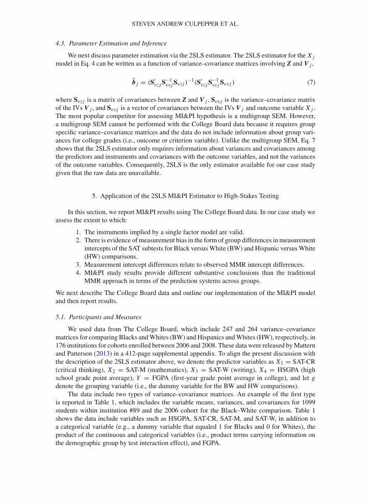
Table 9.Type I error and power rates of ML and 2SLS estimators for latent prediction intercept difference, β01 − β00, by n, p,rxx .

n p rxx β01 − β00 = 0 β01 − β00 = −0.25 β01 − β00 = −0.50


250 0.1 0.5 a 0.033 a 0.178 a 0.531500 0.1 0.5 a 0.035 a 0.309 a 0.7801000 0.1 0.5 0.049 0.035 0.675 0.530 0.983 0.940250 0.3 0.5 0.052 0.042 0.479 0.377 0.931 0.855500 0.3 0.5 0.052 0.043 0.749 0.624 0.995 0.9741000 0.3 0.5 0.051 0.042 0.942 0.866 1.000 0.999250 0.5 0.5 0.052 0.048 0.555 0.460 0.970 0.922500 0.5 0.5 0.051 0.049 0.830 0.724 0.999 0.9941000 0.5 0.5 0.052 0.049 0.978 0.936 1.000 1.000250 0.1 0.7 a 0.043 a 0.235 a 0.662500 0.1 0.7 0.051 0.042 0.477 0.408 0.933 0.8911000 0.1 0.7 0.050 0.043 0.750 0.670 0.995 0.986250 0.3 0.7 0.052 0.048 0.556 0.490 0.970 0.944500 0.3 0.7 0.051 0.046 0.826 0.761 0.999 0.9971000 0.3 0.7 0.051 0.046 0.975 0.951 1.000 1.000250 0.5 0.7 0.053 0.051 0.645 0.585 0.992 0.980500 0.5 0.7 0.050 0.049 0.898 0.852 1.000 1.0001000 0.5 0.7 0.051 0.049 0.993 0.983 1.000 1.000250 0.1 0.9 0.053 0.051 0.303 0.289 0.785 0.765500 0.1 0.9 0.052 0.050 0.524 0.501 0.960 0.9511000 0.1 0.9 0.051 0.049 0.799 0.777 0.998 0.997250 0.3 0.9 0.053 0.051 0.609 0.587 0.985 0.981500 0.3 0.9 0.052 0.051 0.871 0.855 1.000 1.0001000 0.3 0.9 0.050 0.048 0.987 0.983 1.000 1.000250 0.5 0.9 0.052 0.052 0.705 0.686 0.997 0.996500 0.5 0.9 0.051 0.050 0.934 0.924 1.000 1.0001000 0.5 0.9 0.050 0.050 0.997 0.996 1.000 1.000

There were 2187 parameter combinations that were each replicated 5000 times. ML =maximum likelihood estimator, 2SLS = two-stage least squares instrumental variables estimator.aConditions where ML did not converge for at least one replication. β01 − β00 denotes group differences inprediction intercepts, n is sample size, p is the proportion of members in the focal group, and rxx denotespredictor reliability.

Type I error rates. Furthermore, the power to detect group measurement intercept differences wasaffected by n, p, and rxx . In general, power was larger for ML than 2SLS, but the differencebetween the methods declined as τ21 − τ20, n, p, and rxx increased.

Tables 9 and 10 report Type I error rates and power for the ML and 2SLS tests of groupdifferences in latent prediction intercepts (i.e., β01 − β00) and latent slopes (i.e., β11 − β10).Similar to the results in Table 8, the ML and 2SLS estimators controlled the Type I error rateat the a priori level and ML tended to be more powerful than 2SLS across parameter values.Additionally, the power to detect latent prediction intercept differences tended to be larger thanthe power to detect latent slope differences.

In short, results summarized in Tables 8, 9, and 10 support the use of the 2SLS estimatorto perform MI&PI studies. Reassuringly, statistical power for the 2SLS estimator was satisfac-

PSYCHOMETRIKA

Table 10.Type I error and power rates of ML and 2SLS estimators for latent score slope differences, β11 − β10, by n, p, rxx .

n p rxx β11 − β10 = 0 β11 − β10 = −0.125 β11 − β10 = −0.25


250 0.1 0.5 a 0.044 a 0.087 a 0.188500 0.1 0.5 a 0.047 a 0.120 a 0.3111000 0.1 0.5 0.048 0.049 0.277 0.177 0.748 0.522250 0.3 0.5 0.050 0.045 0.183 0.120 0.532 0.350500 0.3 0.5 0.050 0.046 0.307 0.195 0.815 0.6001000 0.3 0.5 0.049 0.049 0.526 0.334 0.979 0.876250 0.5 0.5 0.051 0.045 0.196 0.127 0.597 0.409500 0.5 0.5 0.050 0.048 0.341 0.219 0.881 0.6951000 0.5 0.5 0.050 0.048 0.591 0.387 0.994 0.938250 0.1 0.7 a 0.051 a 0.107 a 0.266500 0.1 0.7 0.049 0.050 0.193 0.157 0.557 0.4511000 0.1 0.7 0.050 0.051 0.325 0.258 0.840 0.730250 0.3 0.7 0.053 0.050 0.215 0.173 0.627 0.521500 0.3 0.7 0.051 0.050 0.368 0.291 0.893 0.8071000 0.3 0.7 0.052 0.050 0.628 0.510 0.995 0.978250 0.5 0.7 0.053 0.052 0.240 0.192 0.701 0.600500 0.5 0.7 0.052 0.050 0.421 0.337 0.941 0.8801000 0.5 0.7 0.051 0.051 0.699 0.584 0.999 0.993250 0.1 0.9 0.051 0.052 0.131 0.125 0.364 0.343500 0.1 0.9 0.051 0.051 0.212 0.200 0.622 0.5861000 0.1 0.9 0.051 0.051 0.368 0.343 0.893 0.868250 0.3 0.9 0.053 0.053 0.241 0.226 0.695 0.664500 0.3 0.9 0.052 0.052 0.416 0.390 0.935 0.9181000 0.3 0.9 0.050 0.051 0.695 0.661 0.999 0.998250 0.5 0.9 0.053 0.053 0.273 0.257 0.768 0.741500 0.5 0.9 0.051 0.051 0.479 0.451 0.967 0.9581000 0.5 0.9 0.051 0.051 0.772 0.739 1.000 0.999

Note. There were 2187 parameter combinations that were each replicated 5000 times. ML =maximum likelihood estimator, 2SLS = two-stage least squares instrumental variables estimator.aConditions where ML did not converge for at least one replication. β11 − β10 denotes group differencesin slope coefficients, n is sample size, p is the proportion of members in the focal group, and rxx denotespredictor reliability.

tory for parameter conditions typically found in high-stakes testing contexts (e.g., n > 500and rxx > 0.7).

References

Aguinis, H. (2004). Regression analysis for categorical moderators. New York: Guilford.Aguinis, H. (2019). Performance management (4th ed.). Chicago, IL: Chicago Business Press.Aguinis, H., Cortina, J. M., & Goldberg, E. (1998). A new procedure for computing equivalence bands in personnel

selection. Human Performance, 11, 351–365.Aguinis, H., Culpepper, S. A., & Pierce, C. A. (2010a). Revival of test bias research in preemployment testing. Journal

of Applied Psychology, 95, 648–680.Aguinis, H., Culpepper, S. A., & Pierce, C. A. (2016). Differential prediction generalization in college admissions testing.

Journal of Educational Psychology, 108, 1045–1059.Aguinis, H., Werner, S., Abbott, J. L., Angert, C., Park, J. H., & Kohlhausen, D. (2010b). Customer-centric science:

Reporting significant research results with rigor, relevance, and practical impact in mind. Organizational ResearchMethods, 13, 515–539.


Albano, A. D., & Rodriguez, M. C. (1998). Examining differential math performance by gender and opportunity to learn.Educational and Psychological Measurement, 73, 836–856.

AmericanEducationalResearchAssociation,AmericanPsychologicalAssociation, andNationalCouncil onMeasurementin Education. (2014). Standards for educational and psychological testing. Washington, DC: American EducationalResearch Association.

Aronson, J., & Dee, T. (2012). Stereotype threat in the real world. In T. Schmader &M. Inzlicht (Eds.), Stereotype threat:Theory, process, and application (pp. 264–278). Oxford: Oxford University Press.

Bernerth, J., & Aguinis, H. (2016). A critical review and best-practice recommendations for control variable usage.Personnel Psychology, 69, 229–283.

Berry, C. M., & Zhao, P. (2015). Addressing criticisms of existing predictive bias research: Cognitive ability test scoresstill overpredict African Americans’ job performance. Journal of Applied Psychology, 100, 162–179.

Birnbaum, Z. W., Paulson, E., & Andrews, F. C. (1950). On the effect of selection performed on some coordinates of amulti-dimensional population. Psychometrika, 15, 191–204.

Bollen, K. A. (1996). An alternative two stage least squares (2SLS) estimator for latent variable equations. Psychometrika,61, 109–121.

Bollen, K.A., Kolenikov, S., &Bauldry, S. (2014).Model-implied instrumental variable—generalizedmethod ofmoments(MIIV-GMM) estimators for latent variable models. Psychometrika, 79, 20–50.

Bollen, K. A., & Maydeu-Olivares, A. (2007). A polychoric instrumental variable (PIV) estimator for structural equationmodels with categorical variables. Psychometrika, 72, 309–326.

Bollen, K. A., & Paxton, P. (1998). Two-stage least squares estimation on interaction effects. In R. E. Schumacker & G.A. Marcoulides (Eds.), Interaction and nonlinear effects in structural equation modeling (pp. 125–151). Mahwah,NJ: Lawrence Erlbaum Associates.

Borsboom, D. (2006). The attack of the psychometricians. Psychometrika, 71, 425–440.Borsboom, D., Romeijn, J. W., & Wicherts, J. M. (2008). Measurement invariance versus selection invariance: Is fair

selection possible? Psychological Methods, 13, 75–98.Browne, M. W., & Cudeck, R. (1992). Alternative ways of assessing model fit. Sociological Methods & Research, 21,

230–258.Bryant, D. (2004). The effects of differential item functioning on predictive bias. Unpublished doctoral dissertation),

University of Central Florida, Orlando, Florida.Cleary, T. A. (1968). Test bias: Prediction of grades of Negro and white students in integrated colleges. Journal of

Educational Measurement, 5, 115–124.Coyle, T. R., & Pillow, D. R. (2008). SAT and ACT predict college GPA after removing g. Intelligence, 36, 719–729.Coyle, T. R., Purcell, J. M., Snyder, A. C., & Kochunov, P. (2013). Non-g residuals of the SAT and ACT predict specific

abilities. Intelligence, 41, 114–120.Coyle, T. R., Purcell, J. M., Snyder, A. C., & Richmond, M. C. (2014). Ability tilt on the SAT and ACT predicts specific

abilities and college majors. Intelligence, 46, 18–24.Culpepper, S. A. (2010). Studying individual differences in predictability with gamma regression and nonlinear multilevel

models. Multivariate Behavioral Research, 45, 153–185.Culpepper, S. A. (2012a). Using the criterion-predictor factor model to compute the probability of detecting prediction

bias with ordinary least squares regression. Psychometrika, 77, 561–580.Culpepper, S. A. (2012b). Evaluating EIV, OLS, and SEM estimators of group slope differences in the presence of

measurement error: The single indicator case. Applied Psychological Measurement, 36, 349–374.Culpepper, S. A. (2016). An improved correction for range restricted correlations under extreme, monotonic quadratic

nonlinearity and heteroscedasticity. Psychometrika, 81, 550–564.Culpepper, S. A., & Aguinis, H. (2011). Using analysis of covariance (ANCOVA) with fallible covariates. Psychological

Methods, 16, 166–178.Culpepper, S. A., & Davenport, E. C. (2009). Assessing differential prediction of college grades by race/ethnicity with a

multilevel model. Journal of Educational Measurement, 46, 220–242.Fan, X., & Sivo, S. A. (2005). Sensitivity of fit indexes to misspecified structural or measurement model components:

Rationale of two-index strategy revisited. Structural Equation Modeling, 12, 343–367.Fischer, F. T., Schult, J., &Hell, B. (2013a). Sex-specific differential prediction of college admission tests: Ameta-analysis.

Journal of Educational Psychology, 105, 478–488.Fischer, F., Schult, J., & Hell, B. (2013b). Sex differences in secondary school success: Why female students perform

better. European Journal of Psychology of Education, 28, 529–543.Gottfredson, L. S. (1988). Reconsidering fairness: Amatter of social and ethical priorities. Journal of Vocational Behavior,

33, 293–319.Gottfredson, L. S., & Crouse, J. (1986). Validity versus utility of mental tests: Example of the SAT. Journal of Vocational

Behavior, 29, 363–378.Hägglund, G. (1982). Factor analysis by instrumental variables methods. Psychometrika, 47, 209–222.Hayashi, F. (2000). Econometrics. Princeton, NJ: Princeton University Press.Hausman, J. A., Newey, W. K., Woutersen, T., Chao, J. C., & Swanson, N. R. (2012). Instrumental variable estimation

with heteroskedasticity and many instruments. Quantitative Economics, 3, 211–255.Hong, S., & Roznowski, M. (2001). An investigation of the influence of internal test bias on regression slope. Applied

Measurement in Education, 14, 351–368.Hu, L. T., & Bentler, P. M. (1999). Cutoff criteria for fit indexes in covariance structure analysis: Conventional criteria

versus new alternatives. Structural Equation Modeling: A Multidisciplinary Journal, 6, 1–55.

PSYCHOMETRIKA

Humphreys, L. G. (1952). Individual differences. Annual Review of Psychology, 3, 131–150.Jöreskog, K. G. (1971). Simultaneous factor analysis in several populations. Psychometrika, 36, 409–426.Jöreskog, K. G. (1998). Interaction and nonlinear modeling: Issues and approaches. In R. E. Schumacker & G. A.

Marcoulides (Eds.), Interaction and nonlinear effects in structural equation modeling (pp. 239–250). Mahwah, NJ:Lawrence Erlbaum Associates Inc.

Keiser, H. N., Sackett, P. R., Kuncel, N. R., & Brothen, T. (2016). Why women perform better in college than admis-sion scores would predict: Exploring the roles of conscientiousness and course-taking patterns. Journal of AppliedPsychology, 101, 569–581.

Kling, K. C., Noftle, E. E., & Robins, R. W. (2012). Why do standardized tests underpredict women’s academic perfor-mance? The role of conscientiousness. Social Psychological and Personality Science, 4, 600–606.

Lance, C. E., Beck, S. S., Fan, Y., & Carter, N. T. (2016). A taxonomy of path-related goodness-of-fit indices andrecommended criterion values. Psychological Methods, 21, 388–404.

Loevinger, J. (1957). Objective tests as instruments of psychological theory. Psychological Reports, 3, 635–694.Lord, F. M., & Novick, M. R. (1968). Statistical theories of mental test scores. Charlotte: Information Age Publishing

Inc.MacCallum, R. C., Browne, M. W., & Sugawara, H. M. (1996). Power analysis and determination of sample size for

covariance structure modeling. Psychological Methods, 1, 130–149.Marsh, H. W., Wen, Z., & Hau, K. (2004). Structural equation models of latent interactions: Evaluation of alternative

estimation strategies and indicator construction. Psychological Methods, 9, 275–300.Mattern, K. D., & Patterson, B. F. (2013). Test of slope and intercept bias in college admissions: A response to Aguinis,

Culpepper, and Pierce (2010). Journal of Applied Psychology, 98, 134–147.McDonald, R. P., & Ho, M. H. R. (2002). Principles and practice in reporting structural equation analyses. Psychological

Methods, 7, 64–82.Meredith, W. (1993). Measurement invariance, factor analysis and factorial invariance. Psychometrika, 58, 525–543.Millsap, R. E. (1995). Measurement invariance, predictive invariance, and the duality paradox. Multivariate Behavioral

Research, 30, 577–605.Millsap, R. E. (1997). Invariance inmeasurement and prediction: Their relationship in the single-factor case.Psychological

Methods, 2, 248–260.Millsap, R. E. (1998). Group differences in regression intercepts: Implications for factorial invariance. Multivariate

Behavioral Research, 33, 403–424.Millsap, R. E. (2007). Invariance in measurement and prediction revisited. Psychometrika, 72, 461–473.Millsap, R. E. (2011). Statistical approaches to measurement invariance. New York: Routledge.Moulder, B. C., & Algina, J. (2002). Comparison of methods for estimating and testing latent variable interactions.

Structural Equation Modeling, 9, 1–19.Muthén, B. O. (1989). Factor structure in groups selected on observed scores. British Journal of Mathematical and

Statistical Psychology, 42, 81–90.Muthén, B., Kaplan, D., & Hollis, M. (1987). On structural equation modeling with data that are not missing completely

at random. Psychometrika, 52, 431–462.Nestler, S. (2014). How the 2SLS/IV estimator can handle equality constraints in structural equation models: A system-

of-equations approach. British Journal of Mathematical and Statistical Psychology, 67, 353–369.Nguyen, H. H. D., & Ryan, A. M. (2008). Does stereotype threat affect test performance of minorities and women? A

meta-analysis of experimental evidence. Journal of Applied Psychology, 93, 1314–1334.Nye, C. D., & Drasgow, F. (2011). Assessing goodness of fit: Simple rules of thumb simply do not work. Organizational

Research Methods, 14, 548–570.Oczkowski, E. (2002). Discriminating between measurement scales using nonnested tests and 2SLS: Monte Carlo evi-

dence. Structural Equation Modeling, 9, 103–125.Olea, M. M., & Ree, M. J. (1994). Predicting pilot and navigator criteria: Not much more than g. Journal of Applied

Psychology, 79, 845–851.Ployhart, R. E., Schmitt, N., & Tippins, N. T. (2017). Solving the supreme problem: 100 years of recruitment and selection

research. Journal of Applied Psychology, 102, 291–304.Rabe-Hesketh, S., Skrondal,A.,&Pickles,A. (2004).Generalizedmultilevel structural equationmodeling.Psychometrika,

69, 167–190.Ree, M. J., & Earles, J. A. (1991). Predicting training success: Not muchmore than g. Personnel Psychology, 44, 321–332.Ree, M. J., Earles, J. A., & Teachout, M. S. (1994). Predicting job performance: Not much more than g. Journal of Applied

Psychology, 79, 518–524.Sackett, P. R., & Ryan, A. M. (2011). Concerns about generalizing stereotype threat research findings to operational

high-stakes testing settings. In T. Schmader &M. Inzlicht (Eds.), Stereotype threat: Theory, process, and application(pp. 246–259). Oxford: Oxford University Press.

Schmitt, N., Keeney, J., Oswald, F. L., Pleskac, T., Quinn, A., Sinha, R., et al. (2009). Prediction of 4-year college studentperformance using cognitive and noncognitive predictors and the impact of demographic status on admitted students.Journal of Applied Psychology, 94, 1479–1497.

Schult, J., Hell, B., Päßler, K., & Schuler, H. (2013). Sex-specific differential prediction of academic achievement byGerman ability tests. International Journal of Selection and Assessment, 21, 130–134.

Society for Industrial and Organizational Psychology. (2018). Principles for the validation and use of personnel selectionprocedures (5th ed.). Washington, DC: American Psychological Association.


Sörbom, D. (1974). A general method for studying differences in factor means and factor structure between groups.BritishJournal of Mathematical and Statistical Psychology, 27, 229–239.

Sörbom, D. (1978). An alternative to the methodology for analysis of covariance. Psychometrika, 43, 381–396.Steele, C. M. (2011). Whistling Vivaldi: How stereotypes affect us and what we can do. New York: WW Norton &

Company.Vandenberg, R. J., & Lance, C. E. (2000). A review and synthesis of the measurement invariance literature: Suggestions,

practices, and recommendations for organizational research. Organizational Research Methods, 3, 4–70.Viswesvaran, C., Ones, D. S., & Schmidt, F. L. (1996). Comparative analysis of the reliability of job performance ratings.

Journal of Applied Psychology, 81, 557–574.Walton, G. M., Murphy, M. C., & Ryan, A. M. (2015). Stereotype threat in organizations: Implications for equity and

performance. Annual Review of Organizational Psychology and Organizational Behavior, 2, 523–550.Wicherts, J. M., & Millsap, R. E. (2009). The absence of underprediction does not imply the absence of measurement

bias. American Psychologist, 64, 281–283.Wicherts, J. M., Dolan, C. V., & Hessen, D. J. (2005). Stereotype threat and group differences in test performance: A

question of measurement invariance. Journal of Personality and Social Psychology, 89, 696–716.Widaman, K. F., & Thompson, J. S. (2003). On specifying the null model for incremental fit indices in structural equation

modeling. Psychological Methods, 8, 16–37.Wu, W., West, S. G., & Taylor, A. B. (2009). Evaluating model fit for growth curve models: Integration of fit indices from

SEM and MLM frameworks. Psychological Methods, 14, 183–201.Young, J. W. (1991a). Gender bias in predicting college academic performance: A new approach using item response

theory. Journal of Educational Measurement, 28, 37–47.Young, J. W. (1991b). Improving the prediction of college performance of ethnic minorities using the IRT-based GPA.

Applied Measurement in Education, 4, 229–239.Zwick, R., & Himelfarb, I. (2011). The effect of high school socioeconomic status on the predictive validity of SAT scores

and high school grade-point average. Journal of Educational Measurement, 48, 101–121.

Manuscript Received: 18 OCT 2017

Documents

s11336-018-9649-2hermanaguinis.com/Psychometrika.pdf · 162 factor variances are a form of heteroscedasticity and prior research considered instrumental vari-163 ′ 2 2 9649. proof