SUMMARY MATERIALS engineering, science, processing and design third edition 

 

Michael Ashby, Hugh Shercliff and David Cebon 

 

 

Bas Comuth

Last edit: 19-1-2019 Disclaimer This document was prepared as a summary for myself. However, it might be useful for other students as well, which is why it was published online. No rights can be claimed, the author is not responsible for any wrong information spread through this document, or the lack of

any information. Also, the author is not affiliated to TU Delft in any other kind than being a student.

Contents

Chapter 1 3 1.1 Materials, processes and choice 4 1.2 Material properties 4 1.3 Design-limiting properties 5

Chapter 2 6 2.1 Introduction and synopsis 7 2.2 Getting materials organised: the materials tree 7 2.3 Organising processes: the process tree 7 2.4 Process-property interaction 8 2.5 Material property charts 8 2.6 Computer-aided information management for materials and processes 8

Chapter 3 9 3.1 Introduction and synopsis 10 3.2 The design process 10 3.3 Material and process information for design 10 3.4 The strategy: translation, screening, ranking and documentation 10

Chapter 4 12 4.1 Introduction and synopsis 13 4.2 Density, stress, strain and moduli 13 4.3 The big picture: material property charts 15 4.4 The science: what determines stiffness and density 15 4.5 Manipulating the modulus and density 18 4.6 Acoustic properties 19

Chapter 5 21 5.1 Introduction and synopsis 22 5.2 Standard solutions to elastic problems 22 5.3 Material indices for elastic design 24 5.4 Plotting limits and indices on charts 26 5.5 Case studies 26

Chapter 6 27 6.1 Introduction and synopsis 28 6.2 Strength, plastic work and ductility: definition and measurement 28 6.3 The big picture: charts for yield strength 29 6.4 Drilling down: the origins of strength and ductility 29 6.5 Manipulating strength 31

Chapter 7 33 7.1 Introduction and synopsis 34

1

7.2 Standard solutions to plastic problems 34 7.3 Material indices for yield-limited design 35 7.4 Case studies 36

Chapter 8 37 8.1 Introduction and synopsis 38 8.2 Strength and toughness 38 8.3 The mechanics of fracture 38 8.4 Material property charts for toughness 39 8.5 Drilling down: the origins of toughness 40 8.6 Compressive and tensile failure of ceramics 40 8.7 Manipulating properties: the strength-toughness trade-off 41

Chapter 9 42 9.1 Introduction and synopsis 43 9.2 Vibration and resonance: the damping coefficient 43 9.3 Fatigue 43 9.4 Charts for endurance limit 44 9.5 Drilling down: the origins of damping and fatigue 44 9.6 Manipulating resistance to fatigue 45

Chapter 10 46 10.1 Introduction and synopsis 47 10.2 Standard solutions to fracture problems 47 10.3 Material indices for fracture-safe design 47 10.4 Case studies 47

Chapter 12 49 12.1 Introduction and synopsis 50 12.2 Thermal properties: definition and measurement 50 12.3 The big picture: thermal property charts 50 12.4 Drilling down: the physics of thermal properties 51 12.5 Manipulating thermal properties 51 12.6 Design and manufacture: using thermal properties 52

Chapter 13 54 13.1 Introduction and synopsis 55 13.2 The temperature dependence of material properties 55 13.3 Charts for creep behaviour 56 13.4 The science: diffusion 56

2

Chapter 1 Introduction: Materials - history and character

3

1.1 Materials, processes and choice Engineers make things. They make them out of materials, and they shape, join and finish them using processes.

1.2 Material properties Properties of materials that have something to do with carrying a load safely are called mechanical properties. One of those properties is stiffness, or resistance to bending if you like, and it is represented by the elastic modulus E. Another one is strength, or the ease with which a material can by permanently bent. Metals have a yield strength σy at which they will plastically deform. When metals deform, they generally get stronger (work hardening), but there is an ultimate limit, called the tensile strength σts, beyond which the material fails. High hardness H gives scratch resistance and resistance to wear. The resistance of materials to cracking and fracture is measured by the fracture toughness K1c. One obvious material property is density ρ, or mass per unit volume. A material also has thermal properties. It has a maximum service temperature Tmax, above which its use is impractical. Most materials expand when they are heated, but by differing amounts depending on their thermal expansion coefficient α. Thermal conductivity λ, measures the rate at which heat flows through the material when one side is hot and the other cold. Heat capacity Cp measures the amount of heat that it takes to make the temperature of material rise by a given amount. The thermal diffusivity a is how quickly the heat will spread through a material, and it is proportional to λ/Cp. Let us now look at electrical, magnetic and optical properties. Electrical conductivity κe, how easy it is for an electric current to flow through a material, and its inverse resistivity ρe, how hard it is for an electric current to flow through a material, are both electrical properties. Dielectric properties are in some cases important to consider. Materials with a high dielectric constant εD have electrons which are very sensitive to an electric field. Materials that have the capacity to trap a magnetic field permanently are called ferri-magnets and ferro-magnets. We will consider two magnetic properties in this chapter: remanence and saturation magnetization. Remanence measures how easily a material can be demagnetized, once magnetized. Saturation magnetization measures how large a field the material can conduct. Materials can also respond to light. Opaque materials reflect light, transparent materials refract it and some materials have the ability to absorb certain wavelengths. Let’s move on to chemical properties. We regard the intrinsic resistance of a material to for instance corrosion (oxidation), organic solvents, acids and alkalis or ultra-violet radiation as material properties, measured on a scale of 1 (very poor) to 5 (very good).

4

Last but certainly not least we have environmental properties. An engineer must also consider material efficiency and sustainability, and also the sustainability of the processes needed to fabricate these materials.

1.3 Design-limiting properties The performance of a component is limited by certain of the properties of the materials of which it is made. This means that, to achieve a desired level of performance, the values of the design-limiting properties must meet certain targets, and those that fail to do so are not suitable.

5

Chapter 2 Family trees: organising materials and processes

6

2.1 Introduction and synopsis Processes and materials can be organised in families. Family likenesses are most strikingly seen in material property charts. Another way of organising materials or processes is classification.

2.2 Getting materials organised: the materials tree It is conventional to classify the materials of engineering into the six broad families: metals, polymers, elastomers, ceramics, glasses and hybrids (composite materials made by combining two or more of the other families). Families can be expanded to show classes, sub-classes and members, each of which is characterised by its properties. Metals are characterised by relatively high stiffness, fracture toughness and electrical and thermal conductivity. Most when pure have a low yield strength, which can be increased by hardening them. They will remain ductile. Metals are also very reactive, and corrode rapidly. Ceramics are non-metallic, inorganic solids. They are stiff, hard abrasion-resistant (a high maximum service temperature), they resist corrosion well and they are good electrical insulators. However, they have a low fracture toughness. Glasses are non-crystalline (amorphous) solids. They are hard and remarkably corrosion resistant. Glasses are excellent electrical insulators and are transparent to light. On the other hand glasses are very brittle and vulnerable to stress concentrations. Polymers are organic solids based on long chains of carbon atoms. They are light, have a low stiffness, a low service temperature and easy to shape. They can be strong though, and because of their low density, their specific strength (strength per unit weight) is surprisingly high. Elastomers are polymers with the unique property that their stiffness is extremely low, which causes them to be able to be stretched to many times their starting length. Despite this property they can be strong and tough. Hybrids are combinations of two or more materials in an attempt to get the best of both. This causes them to have attractive properties. Nonetheless they are expensive and relatively difficult to form and join.

2.3 Organising processes: the process tree A process is a method of shaping, joining or finishing a material. The choice of a process will be based on the design requirements and the type of material. Manufacturing processes are organised in: primary shaping, secondary processes, joining and surface

7

treatment (primary shaping and secondary processes both belong to the family ‘shaping’). Examples of the first are casting, molding, deformation, powder methods, composite forming or other special methods. Secondary processes are machining and heat treatment. Some joining methods are fastening, riveting, welding, heat bonding, snap fits, friction bonds, adhesives cements. Examples of the latter are polishing, texturing, plating, metallizing, anodizing, chromizing, painting and printing.

2.4 Process-property interaction Both processing and joining can change the properties of the materials.

2.5 Material property charts A way to put materials in perspective and compare them is to use material property charts (either bar charts or bubble charts). In most charts a logarithmic scale is used. A bar chart is used to plot one physical quantity, a bubble chart to plot two. These charts are often used in the studies of materials.

2.6 Computer-aided information management for materials and processes Materials and processes can also by organised in computer systems.

8

Chapter 3 Strategic thinking: matching material to design

9

3.1 Introduction and synopsis Design starts with a market need, which is analysed and expressed as design requirements. Concepts then are sought, developed (embodied), and refined (detailed) to give a product specification. Selection strategy involves translation, screening, ranking and documentation.

3.2 The design process Original design starts from a new concept and develops the information necessary to implement it. Evolutionary design or redesign starts with an existing product and seeks to change it in ways that increase its performance or/and reduce its cost. Some scenarios that call for redesign are:

- Product recall: if a product, once released to the market, fails to meet safety standards, urgent redesign is required.

- Poor value for money: the product performs safely but offers performance that, at its price, is perceived to be mediocre, requiring redesign to enhance performance.

- Inadequate profit margin: the cost of manufacture exceeds the price that the market will bear.

- Sustainable technology: the response of the designer to the profligate use of materials in products and packaging, and to consumer pressure for production that does not harm the environment.

- Mac-effect: in a market environment in which many almost-identical products compete for the consumer’s attention, it is style, image and character (industrial design) that sets some products above others.

3.3 Material and process information for design Selection of process is analogue to and influenced by the selection of materials. It is also influenced by the requirements for shape.

3.4 The strategy: translation, screening, ranking and documentation The first task is that of translation: converting the design requirements into a prescription for selecting a material. This proceeds by identifying the constraint that the material must meet and the objectives that the design must fulfil. The second task, then, is that of screening: eliminating the materials that cannot meet the constraint. This is followed by the ranking step: ordering the survivors by their ability to meet a criterion of excellence, such as that of minimising cost. The final task is to explore the most promising candidates in depth, a step we call documentation. Process selection follows a parallel route, but in that case translation

10

means identifying the geometric and other constraints that must be met. The designer is free to vary dimensions that are not constrained by design requirements and, most importantly, free to choose the material for the component and the process to shape it. We refer to these as free variables.

11

Chapter 4 Stiffness and weight: density and elastic moduli

12

4.1 Introduction and synopsis Stress causes strain. If you are human, the ability to cope with stress without undue strain is called resilience. If you are a material, it is called elastic modulus. Strain, a change of shape is a response to stress (something that is applied to a material by loading it). It depends on the magnitude of the stress and the way it is applied (the mode of loading). Stiffness is the resistance to change of shape that is elastic, meaning that the material returns to its original shape when the stress is removed. Strength is its resistance to permanent distortion or total failure. Both are material properties.

4.2 Density, stress, strain and moduli In most cases, a component can be idealised as one of the simply loaded cases, a tie, column, beam, shaft or shell. Ties carry simple axial tension, columns compression. Bending of a beam creates simple axial tension in elements on one side of the neutral axis and simple compression in those on the other. Pressure difference applied to a shell generates bi-axial tension or compression. Every plane normal to a force F carries that force. If the area of such a plane is A, the tensile stress in the element (neglecting its own weight) is

σ = AF

If the sign of F is reversed, the stress is compressive and given a negative sign. If, instead, the force lies parallel to the face of the element, three other forces are needed to maintain equilibrium. They create a state of shear in the element. Shear stress is given by

τ = AF s

One further state of multi-axial stress is produced by applying equal tensile or compressive forces to all six faces of a cubic element. The state of stress is one of hydrostatic pressure p. Notice that pressures are positive when they ‘push’, the reverse of the convention for simple tension and compression. A tensile stress applied to an element causes the element to stretch. If the element originally of length L0, stretches by δL=L-L0, the nominal tensile strain is

ε = L0

δL A shear stress causes a shear strain γ. If the element shears (sideways) by a distance w, the shear strain is

an(γ)t = wL0

≈ γ Strains are almost always small so it can be assumed that tan(γ)=γ. Finally, a hydrostatic pressure causes an element of volume V to change in volume by δV=V-V0. The volumetric strain or dilatation, is

13

Δ = VδV

Within the linear elastic regime, strain is proportional to stress. This holds for all three types of strain and stress mentioned above. The three relations are

εσ = E γτ = G Δp = K

in which E, G and K are constants of proportionality, respectively called the Young’s modulus, shear modulus and bulk modulus. When stretched in one direction, a element generally contracts in the other two directions. Poisson’s ratio v is the negative of the ratio of the lateral or transverse strain to the axial strain in tensile loading.

−ν = εεt

Since the transverse strain itself is negative, v is positive. In an isotropic material (one for which the moduli do not depend on the direction in which the load is applied) the moduli are related in the following ways:

; G = E2(1+ν) K = E

3(1−2ν) Commonly v≈⅓ so that

; EG = 83 K = E

except for elastomers, for which v≈½ so that

; EG = 31 >K > E

Suppose a cubic element is subjected to three unequal stresses in three different direction (normal to each other). Using the formula for stress on the top of this page for the stress in one direction, then using poisson’s ratio for the stresses in the other two directions and ultimately repeating this for the other stresses and summing the strains, gives us Hooke’s Law in three dimensions

(σ σ σ )ε1 = 1E 1 − ν 2 − ν 3 (− σ σ )ε2 = 1

E ν 1 + σ2 − ν 3 (− σ σ )ε3 = 1

E ν 1 − ν 2 + σ3 If a cube is constrained in a slot, it behaves like a material with an ‘effective modulus’ which is greater than E

ε1

σ1 = E1−ν2

This effect becomes more marked when there are constraints in more directions.

14

If you stretch an elastic band, elastic energy is stored in it. A force acting through a displacement dL does work F*dL. A stress F/A acting through a strain increment dε=dL/L does work per unit volume

W dεd = ALFdL = σ

with units of J/m3. The work done per unit volume as the stress is raised from zero to a final value σ* is the area under the stress-strain curve

dεW = ∫σ*

0σ = ∫

σ*

0E

σdσ = 2E(σ )* 2

The energy is released when the stress is relaxed. Strain can be induced by stress fields, thermal fields, electric fields or magnetic fields.

4.3 The big picture: material property charts Two examples of material property charts are the modulus-density chart and the modulus-relative cost chart. Glasses and most polymers have disordered structures with no particular directionality about the way the atoms are arranged. They have properties that are isotropic, meaning they are the same no matter which direction they are measured. Most materials are crystalline: made up of ordered arrays of atoms. Metals and ceramics are usually polycrystalline: made up of many tiny, randomly oriented crystals. This averages out the directionality in properties. Anisotropy is important though, in single crystals, drawn polymers, fibres and woods.

4.4 The science: what determines stiffness and density The atoms of a metal can be packed in many ways, three of which will be discussed here. They can be seen in figure 1. The CPH-structure has a ABAB… sequence, the third layer is exactly above the first layer, and so on. The FCC-structure has the same packing fraction, but has a ABCABC... sequence. The BCC-structure, which has a lower packing fraction than the two previous structures, consists of atoms packed in squares in an ABAB… sequence. The characterising unit of a crystal structure is called its unit cell. Unit cells pack of fill space, the resulting array is called the crystal lattice. The points at which cell edges meet are called lattice points. The crystal itself is generated by attaching one or a group of atoms to each lattice point so that they form a regular, three-dimensional, repeating pattern.

15

figure 1 Ceramics can have the same ways of packing as metals, with different atoms at different spots. Glasses can be crystalline and amorphous, depending on the ring size. Polymers can occur in many forms. Four of the most important ones are shown in figure 2. Polymers of type A only have weak hydrogen bonds. It is an amorphous thermoplastic. These weak bonds, however, try to keep the bond lengths short by lining the molecules up, resulting in polymers of type B, which are partly crystalline crystallites. Elastomers are polymers of type C, which have very few crosslinks. Thermosets are polymers of type D, which have a lot of crosslinks. The cohesive energy measures the strength of the atomic bonds. It is defined as the energy per mol required to separate the atoms of a solid completely. The atoms have equilibrium spacing a0, and a force can pull them apart a little, to a0+δ. The stiffness then is

S = δF

Relating this to the Young’s modulus can be done as follows

εσ = Sa0

E = S

a0

The bonds between the molecules of an elastomer are weak, so weak that they have melted at room temperature. Segments are free to slide over each other, only limited by the few cross-links. This explains their very low stiffness. The modulus of elastomers increases with temperature, in contrast to the behaviour of all other solids.

16

figure 2 The temperature at which the weak inter-chain bonds of polymers start to melt is called the glass transition temperature Tg. Elastomers and thermosets have a glass transition, but they decompose and burn instead of melt because of the cross-linking. Below Tg, thermoplastics are controlled by hydrogen bonds and referred to as ‘glassy’. Above Tg, amorphous thermoplastics turn into a viscous flow. The degree of crystallinity determines how stiff the material remains above Tg, but eventually all thermoplastics melt and flow. The more a thermoset is cross-linked, the less it shows a glass transition. The glass transition temperature is sensitive to the deformation rate (how fast the material is deformed). The density of a material is mainly determined by the atomic weight and only to a lesser degree by the atom size and the way in which they are packed. The density of a metallic alloy can be determined using the rule of mixtures

ϱ 1 )ϱ ϱalloy = f A + ( − f B where f is the volume fraction of A atoms.

17

4.5 Manipulating the modulus and density Composites are made by embedding fibres or particles (possible in many ways, see figure 3) in a continuous matrix of a polymer (PMC’s), a metal (MMC’s) or a ceramic (CMC’s).

figure 3 The density of a composite, provided that it is a composite with no residual porosity, can be calculated as follows (the matrix and reinforcement are respectively denoted by the subscripts m and r and f is the volume fraction of the reinforcement)

ϱ 1 )ϱ ϱcomposite = f r + ( − f m The modulus of a composite is bracketed by two bounds. The upper bound, EU, is found by assuming that on loading the two components strain by the same amount, like springs in parallel

18

E 1 )EEU , composite = f r + ( − f m The lower bound, EL, can be found by assuming that the two components carry the same stress, like springs in series.

EL, composite = E Em rfE +(1−f )Em r

figure 4 Figure 4 shows an idealised cell of a low-density foam. It consists of solid cell walls or edges surrounding a void containing a gas.

)ϱsolid

ϱfoam = ( tL2

)Esolid

Efoam = ( ϱsolidϱfoam 2

4.6 Acoustic properties Sound is transmitted through materials as an elastic wave. The wavelength λ is related to the frequency f by

f = λv

where v is the velocity of sound in the medium in which it is travelling. The longitudinal sound velocity in a long rod of a solid material, such that the thickness is small compared with the wavelength, is

v1 = √ ϱE

19

If the thickness of the rod is large compared with the wavelength, the velocity, instead, is

vB = √ E(1−ν)(1−ν−2ν )ϱ2

Elastically anisotropic solids have sound velocities which depend on direction

v//v⊥

= √ E//E⊥

Sound power, even for very loud noise, is small. The proportion of sound absorbed by a surface is called the sound-absorption coefficient. The degree of insulation (keeping sound from outside, outside) is proportion to the mass of the wall, floor or roof through which sound has to pass. This is known as the mass-law. If a sound-transmitting material is interfaced with a second one with different properties, part of the amplitude of the sound wave is transmitted across the interface and part is reflected back into the first material. This is determined by the sound wave impedance

Z = √ϱE The reflection coefficient R is the fraction of the acoustic energy that is reflected, given

)R = ( Z +Z2 1

Z −Z2 1 2 where Z1 is the impedance in the medium in which the sound originates and Z2 is that of the material into which it is transmitted. The energy that is not reflected is transmitted, so the transmission coefficient T is

T = 1 − R = 4Z Z1 2

(Z +Z )2 12

The intensity of sound radiation I scales with modulus and density as

∝ I √ Eϱ3

The factor in the right half of this proportion is called the radiation factor. When the material is elastically anisotropic, E is replaced by . E = √E E// ⊥

20

Chapter 5 Flex, sag and wobble: stiffness-limited design

21

5.1 Introduction and synopsis Every loading on any real component can be decomposed into some combination of tension, compression, bending and torsion, so it makes sense to have a catalog of solutions regarding stiffness for the standard modes.

5.2 Standard solutions to elastic problems The relation between the load F and deflection δ can be obtained using formulas for stress and strain from chapter 4

δ = AEL F0

The stiffness S for a tie loaded in tension is defined as

S = δF = L0

AE When a beam is loaded by a bending moment M, its initially straight axis is deformed to a curvature κ

κ = dx2d u2

= 1R

where u is the displacement parallel to the y-axis. The stress differs with position y, so that

κyσ = I

M = E = E dx2d u2

where I is the second moment of area. The distance y is measured vertically from the neutral axis (position where the stress is zero). The ratio of moment to curvature is called the flexural rigidity. For a beam of length L with a transverse load F, the stiffness is

S = δF =

L3C EI1

C1 depends on the load type, see figure 5. A torque, T, applied to the ends of an isotropic bar of a uniform section generates a shear stress. For circular section, the shear stress varies with radial distance r from the axis of symmetry is

rτ = T

K where K measures the resistance of the section to twisting (the torsional equivalent to I, for bending). K is equal to the polar second moment of area for circular sections. For non-circular sections, K is less than J. The shear stress causes the bar to twist through an angle θ. It is related to the length, shear stress and torque by

rτ = T

K = LGθ

The ratio of torque to twist is called the torsional rigidity.

22

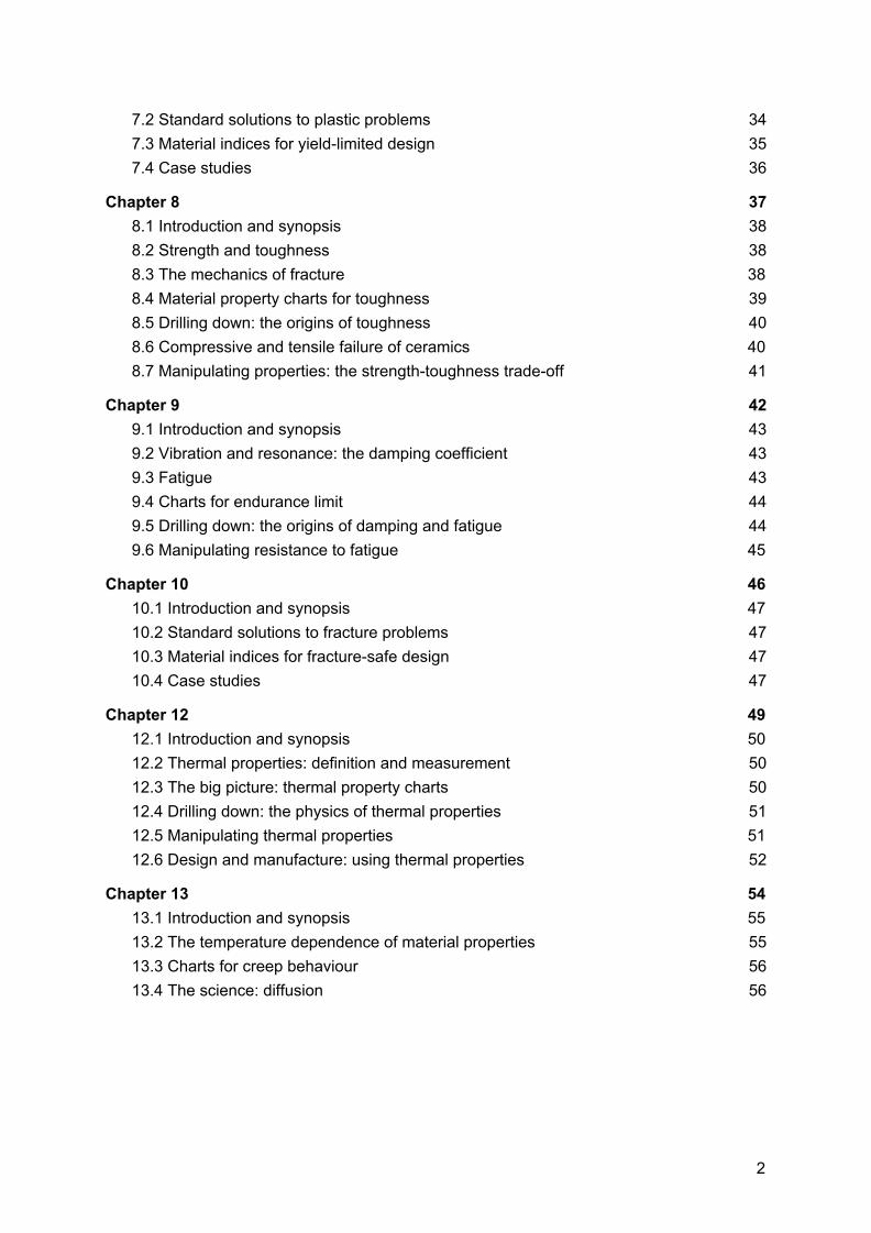
If sufficiently slender, an elastic column or plate, loaded in compression, fails by elastic buckling at a critical load

F crit =L2

n π EI2 2 where n is a constant that depends on the end constraints (see figure 6). It is the number of half-wavelengths of the buckled shape. Any undamped system vibrating at one of its natural frequencies can be reduced to the simple problem of a mass attached to a spring, having a lowest natural frequency

f = 12π√ k

m The lowest natural frequencies of the flexural modes of uniform beams or plates can be calculated as follows, noticing that the spring stiffness is in this case equal to the stiffness S

f = 2πC2√ EI

m Lo 4 where mo is the mass of the beam per unit length: Aρ. C2-values can be seen in figure 5 The natural frequency becomes

f = 2πC2√ I

AL4√ ϱE

Thus frequencies scale as . √E/ϱ

figure 5

23

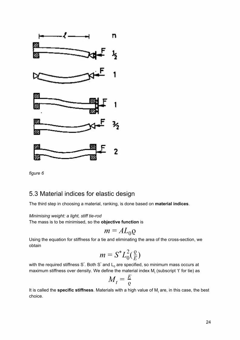
figure 6

5.3 Material indices for elastic design The third step in choosing a material, ranking, is done based on material indices. Minimising weight: a light, stiff tie-rod The mass is to be minimised, so the objective function is

L ϱ m = A 0 Using the equation for stiffness for a tie and eliminating the area of the cross-section, we obtain

L ( )m = S* 20

ϱE

with the required stiffness S*. Both S* and L0 are specified, so minimum mass occurs at maximum stiffness over density. We define the material index Mt (subscript ‘t’ for tie) as

M t = ϱE

It is called the specific stiffness. Materials with a high value of Mt are, in this case, the best choice.

24

Minimising weight: a light, stiff panel The objective function for a panel is

Lϱ hLϱ m = A = b We can use the same method as for a tie, instead using the formula for the stiffness for a bending beam, and the formula for the second moment of area for a rectangular section. Eliminating h yields

) (bL )( )m = ( C b1

12S* 1/3 2 ϱE1/3

Again, the quantities S*, L, b and C1 are all specified, the only freedom of choice left is that of the material. Minimum mass occurs at maximum values of E1/3/ρ. The material index Mp for the panel is

M p = ϱE1/3

Minimising weight: a light, stiff beam The objective function for the mass of a square section beam is

Lϱ m = b2 Now using again the formula for the stiffness of a bending beam, but using the formula for the second moment of area of a square section beam instead of a rectangular section, we get, eliminating b,

) (L)( )m = ( C1

12S L* 3 1/2 ϱE1/2

S*, L and C1 are specified, so the material index Mb for a beam is

M b = ϱE1/2

A rectangular beam does not have the optimum geometry in order to minimise weight. Shaping the cross-section enables an increase in the value of I, without changing A. We therefore introduce the shape factor Φ, defined as the ratio of I for the shaped section to that for a solid square section with the same area A

Φ = IIsquare =

A212I

The deeper and more thin-walled the cross-sectional shape, the larger the value of the shape factor, but there is a limit: make it too thin and the walls will buckle. Moreover, manufacturing limits the maximum achievable thinness. If we fill in the formula for the shape factor in the objective function for the beam, and then eliminate A, we obtain a different resulting performance index

M b = ϱ(ΦE)1/2

Minimising material cost

25

If the material price is Cm $/kg, the cost of the material to make the component is just mCm. The objective function for the material cost C of the tie, panel or beam then becomes

C LC ϱ C = m m = A m Proceeding as in the three previous examples then leads to indices that are the same, with ρ replaced by Cmρ.

5.4 Plotting limits and indices on charts If we take the logs of the material indices for a tie, beam and panel we respectively obtain

og(E) og(ϱ) og(C) l = l + l og(E) log(ϱ) og(C) l = 2 + l og(E) log(ϱ) og(C) l = 3 + l

with C being a constant. These lines one can plot in the E-ρ charts. We refer to these lines as selection guidelines. The methods for selecting materials shown above are practical when there are very few constraint. If there are a lot of factors that are variable, material selection is usually done using computers.

5.5 Case studies The deflection δ that can be seen in figure 4 can be calculated using the following formulas

δ = FL3

C E I1 solid

I = t412

If one redesign something the natural frequencies of that component change. The change in frequency depends on the modulus and density of the new and old material

f Δ = √ E ϱold old

E ϱnew old

26

Chapter 6 Beyond elasticity: plasticity, yielding and ductility

27

6.1 Introduction and synopsis The yield stress is the stress beyond which a material becomes plastic.

6.2 Strength, plastic work and ductility: definition and measurement The yield strength σy (or elastic limit σel) is, for metals, not always clearly determinable. We therefore identify σy with the 0.2% proof stress, that is, the stress at which the stress-strain curve for axial loading deviates by a strain of 0.2% from the linear elastic line. When strained beyond the yield point, most metals work harden, causing the rising part of the curve, until a maximum, the tensile strength σts. This is followed in tension by non-uniform deformation (necking) and fracture. For polymers σy is identified as the stress at which the stress-strain curve becomes markedly non-linear: typically a strain of 1%. The behaviour beyond yield depends on the temperature relative to glass temperature Tg. Well below Tg most polymers are brittle. As Tg is approached, plasticity becomes possible until, at about Tg, thermoplastics exhibit cold drawing: large plastic extension at almost constant stress during which the molecules are pulled into alignment with the direction of straining, followed by hardening and fracture when alignment is complete. At still higher temperatures, thermoplastics become viscous and can be moulded, thermosets become rubbery and finally decompose. Plastic strain, εpl, is the permanent strain resulting from plasticity

εpl = εtot − σE

The ductility is a measure of how much plastic strain a material can tolerate. It is measured in standard tensile tests by the elongation εf (the tensile strain at break) expressed as a percentage. Beyond the elastic limit plastic work is done in deforming a material permanently by yield or crushing. The plastic work per unit volume at fracture is

dεW pl = ∫εf

0σ pl

which is just the area under the stress-strain curve. Ceramics and glasses are brittle at room temperature. They do have yield strengths, but these are so enormously high that they are never reached, the material fractures first. The measure used for ceramics and glasses is the compressive crushing strength. We call it the elastic limit and give it the symbol σel, since it is not true yield even though it is the end of the elastic part. A hardness test can be used instead of tensile and compression tests. Hardness is the load F divided by the area A of the indent, made by the instrument, projected onto a plane

28

perpendicular to the load. A commonly used scale, that of Vickers, uses units of kg/mm2, with the result that

Hv ≈ 3σy

A hardness test is non-destructive, but less accurate. Until now we have only considered nominal stresses and strains. However with stresses, dimensions change, and therefore also the stresses and strains. The formulas for true stress and true strain are, respectively

(1 )σt = σn + εn

ε n(1 )t = ∫L

L0

LdL = l + εn

For the elastic regime and small plastic strains, the difference between nominal and true stresses and strains is negligible.

6.3 The big picture: charts for yield strength Strength can be displayed on material property charts. Two are particularly useful: the strength-density chart and the modulus-strength chart. For strength the yield strength or the elastic limit is used.

6.4 Drilling down: the origins of strength and ductility The distance over which inter-atomic forces act is small: a bond is broken if it is stretched to more than about 10% of its original length. So the force needed to break bond is roughly

F = 10Sa0

On this basis the ideal strength of a solid should therefore be roughly

σideal = E10

More refined calculations give a ratio of 1/15. Crystals contain imperfections of several kinds, which can be seen in figure 7. At the top left are point defects. All crystals contain vacancies: sites at which an atom is missing. At the top right a substitutional solid solution (the dissolved atoms replace those of the host) and a interstitial solid solution (the dissolved atoms squeeze into the spaces between the host atoms) are shown. Both are caused by the creation of alloys: a material in which a second element is dissolved. The different size of the atoms causes distortion in the surrounding lattice. Bottom left a dislocation is displayed. It is dislocations that make metals soft and ductile.

29

figure 7 The bottom right image shows a more drastic defect: grain boundaries. Here three perfect, but differently oriented, crystals meet. The individual crystals are called grains, the meeting surfaces are grain boundaries. A dislocation can be done in two ways. An edge dislocation is made by sliding the top part of the crystal across the bottom (made possible by a cut) by one full atom spacing, and then reattaching the atoms. In this way the dislocation can ‘travel’ through the entire crystal. By the end of the process the upper part has slipped by the slip vector b. The result is shear strain. The upper part of the can also be displaced parallel to the edge of the cut (rather than normal to it). This creates a screw dislocation. All dislocation are either an edge or a screw dislocation, or a mix. In real crystals it is easier to make and move dislocations on some planes than on others. The preferred planes are called slip planes, the preferred directions slip directions. Crystals resist the motion of dislocations with a friction-like resistance f per unit length. For yielding to take place the external stress must overcome f. The force does work

30

L L bW = τ 1 2 L1 and L2 being the dimensions of the plane the shear stress acts on and b being the magnitude of the slip vector. Equating this to the work done by the applied stress gives

bτ = f The atoms near the core of a dislocation are displaced from their proper positions, and thus they have higher potential energy. To keep the potential energy of the crystal as low as possible, the dislocation tries to be as short as possible: it behaves as if it had a line tension T

EbT = 21 2

The resistance to slip ff comes from several factors. First is the lattice resistance fi: the intrinsic resistance of the crystal structure to plastic shear. If this resistance is low, as in metals, the material can be strengthened by introducing obstacles to slip. This is done by adding alloying elements to give solid solution hardening fss, precipitates or dispersed particles giving precipitation hardening fppt, other dislocations giving what is called work hardening fwh or grain boundaries introducing grain-size hardening fgb. Polymers with higher glass temperatures do not draw (see section 6.2 for cold drawing) at room temperature. They craze instead. Small crack-shaped regions within the polymer draw down. Because the crack has a larger volume than the polymer that was there to start with, the drawn material ends up as ligaments that link the craze surfaces. Crazes scatter light, so their presence causes whitening. Crazing limits ductility in tension.

6.5 Manipulating strength Spacing means the distance L between obstacles that contribute to the resistance f in the slip plane. α is a dimensionless constant characterizing obstacle strength. If we roughen the slip plane by solid solution hardening, we add an additional resistance. The concentration of solute atoms is on average

c = b2

L2 The contribution to the shear stress required to move the dislocation then is

Ecτ ss = α 1/2 For precipitation-hardened materials the formula is

τ ppt = bL2T = L

Eb

31

The dislocation density is defined as the length of dislocation line per unit volume. The contribution of the work hardening then is

τwh = 2Eb√ϱd

The contribution of grain boundary hardening depends on the grain size D and the Petch constant: kp

τ gb = kp√D

To a first approximation the strengthening mechanisms add up, giving a shear yield strength

τ y = τ i + τ ss + τ ppt + τwh + τ gb This is the yield strength, to link this to the yield strength of a polycrystalline material in tension in tension, we need another formula.

sinθcosθτ = FsinθA/cosθ = σ

θ being the angle of the normal of the plane of the shear stress, to the axis of tension. For a sample that has many strains

τσy = 3 y Polymers cannot be strengthened by the principles described above. They have to be blended, drawn, cross-linked or reinforced.

32

Chapter 7 Bend and crush: strength-limited design

33

7.1 Introduction and synopsis Strength-limited design, is design to avoid plastic collapse. We want to avoid yielding.

7.2 Standard solutions to plastic problems For ties and columns it is easy. If the stress does not exceed the yield stress, the material will not yield. For bending beam and panels, the maximum stress occurs at the greatest distance ym from the neutral axis. The maximum stress the beam or panel can take before yielding is

σmax = IMym = M

Ze Ze=I/ym and is called the elastic section modulus. Small zones of plasticity appear if the maximum stress is slightly exceeded. As the moment increases further the plastic zones grow until they penetrate through the section of the beam, linking to form a plastic hinge. Further increase causes it to collapse. This failure moment Mf is found by integrating the moment caused by the constant stress distribution over the section

(y)|y|σ dy σM f = ∫

sectionb y = Zp y

Zp being the plastic section modulus. Failure in a shaft occurs when the maximum surface stress exceeds the yield strength of the material. The maximum shear stress is at the surface and has the value

τmax = KTR

The yield stress in shear, k, is half the tensile yield stress, so the maximum torque a shaft can carry before collapsing (for a circular section) is

πR kT = 32 3

Helical springs are a special case of torsional loading. If the spring has n turns of wire of shear modulus G, each of diameter d, wound to give a spring of radius R, the stiffness is

S = uF = Gd4

64nR3 where F is the axial force applied to the spring and u its extension. The elastic extension is limited by the onset of plasticity. This occurs at the force

F crit = 32Rπd σ3

y

34

Spinning disks or rings (flywheels) store kinetic energy U. Centrifugal forces generate a radial tensile stress in the disk that reaches a maximum value. The disk yields when the maximum radial tensile exceeds the yield strength

ϱtω RU = 4π 2 4 .42ϱω R σmax = 0 2 2

Stresses can also occur at contact. Consider a sphere of radius R pressed against a flat surface with a load F. Both sphere and surface have Young’s modulus, Poisson’s ratio is ⅓. The radius of the contact area is

.7( )a ≈ 0 EFR 1/3

The relative displacement of the two bodies is

− )u ≈ ( F2

E R21/3

Yielding first occurs due to shear stress, so

τmax = F2πa2

If this exceeds the shear yield strength k=σy/2, a plastic zone appears beneath the center of the contact. Holes, slots, threads and changes in section concentrate the stress locally. We define the nominal stress in a component as the load divided by the cross-section. The maximum local stress is then found approximately by multiplying the nominal stress by a stress concentration factor Ksc

( )Ksc = σmaxσnom = 1 + α c

ϱsc1/2

Here ρsc is the minimum radius of curvature of the stress-concentrating feature and c is a characteristic dimension associated with it: either the half-thickness of the remaining ligament, the half-length of a contained notch, the length of an edge notch or the height of a shoulder. The factor α is roughly 2 for tension, ½ for torsion and bending.

7.3 Material indices for yield-limited design Minimising weight: a light, strong tie-rod We want to minimise weight, and therefore minimise mass

Lϱ m = A In order to carry the load F without yielding

L( )AF ≤ σy → m ≥ F ϱ

σy The lightest tie that will carry F safely is that made of the material with the smallest value of ρ/σy. As in Chapter 5, defining a material index

35

M t = ϱσy

Minimising weight: light, strong panels We can apply more or less the same method as in Chapter 5 for elastic design. We come to

M p = ϱσy1/2

Light, strong beams: the effect of shape The analysis for a beam is similar to that of the panel. The resulting material index is

M b = ϱσy2/3

The factor for strength is

ΦyB =

Zesolid

Zeshaped

Minimising material cost or volume for strength design works the same as for stiffness design.

7.4 Case studies When a ligament of thickness t is bent elastically to a radius R, the surface strain is

ε = t2R

36

Chapter 8 Fracture and fracture toughness

37

8.1 Introduction and synopsis Toughness is the resistance to fracture. It requires a new material property, the fracture toughness.

8.2 Strength and toughness If one had to design a test to characterise toughness, one would notch it, yank it or whack it till it breaks, measuring the energy to do so. These test though, do not measure a true material property. They are solely used to the purpose of ranking.

8.3 The mechanics of fracture Cracks and notches concentrate stress. The local stress at a distance r from the tip of a crack, caused by a remote uniform tensile stress is

(1 ) σlocal = σ + Y√ πc2πr

where Y is a constant with a value near unity that depends weakly on the geometry of the cracked body. Far from the crack, where r>>c, the local stress falls to the value σ, near the tip, where r<<c, it rises steeply as

σlocal = Y √2πrσ√πc

So for any given value of r the local stress scales as , which therefore is a measure of σ√πc the ‘intensity’ of the local stress field. This quantity is called the mode 1 stress intensity factor K1 (the ‘mode 1’ means tensile loading perpendicular to the crack

σK1 = Y √πc The loading on the crack tip region that drives potential failure is an elastic stress field that scales with K1. As a result cracks propagate when the stress intensity factor exceeds a critical value, the fracture toughness K1c

σK1c = K1 = Y *√πc ≈ σ*√πc It is a material property, so the value is independent of the way it is measured. Important applications of this formula are calculating the failure stress or the critical crack length. When a sample fractures, a new surface is created. Surfaces have energy, the surface energy γ. If you fracture a sample across a cross-section area A you make an area 2A of new surface, requiring an energy of at least 2Aγ joules to do so. Consider first the question of the necessary condition for fracture. It is that sufficient external work be done, or elastic energy released, to at least supply the surface energy of the new surfaces that are created

γG ≥ 2

38

where G is called the energy release rate. Growing a crack costs energy Gc. Gc is called, confusingly, the toughness or the critical strain energy release rate. A slab of material of unit thickness carrying a stress has elastic energy

U v = σ2

2E If we put a crack in it, it releases the stress in a half-cylinder of radius about c releasing the energy it contained

(c)U = 4Eσ πc2 2

Suppose now that the crack extends by δc. The condition for fracture becomes

U δc δcδ = 2Eσ πc2 = Gc

2EK2

1c = Gc This derivative is an approximate one. The correct result we want is

K 1c = √EGc

Gc is also a material property. The intense stress field at the tip of a crack generates a process zone: a plastic zone in ductile solids, a zone of micro-cracking in ceramics, a zone of delamination, debonding and fibre pull-out in composites. The radius of the plastic zone, allowing for stress redistribution is

( )ry = 2 σ πc2

2πσy2= K2

1πσy2

When cracks are small, materials yield before they fracture, when they are large, the opposite is true. Above the critical crack length materials fracture, below they yield

ccrit = K21c

πσy2

The stress at which the material fractures is

σf = K1cπσy2

8.4 Material property charts for toughness Fracture toughness can be plotted in two charts. In the fracture toughness-modulus chart, the toughness Gc is incorporated using straight lines. In the fracture toughness-strength the transition crack length can be incorporated in the same way.

39

8.5 Drilling down: the origins of toughness An energy of at least 2γ is needed to cut a material. The atoms are bonded on all sides so the surface atoms lose one-sixth of their bonds when the cut is made. This means that we have to provide one-sixth of the cohesive energy Hc to a slice 4r0 thick, where ro is the atom radius. So the surface energy should be

H rγ = 31

c o Hc is typically 3 x 1010 J/m3 and r0 1010 m. Gc is often way larger than 2γ, the extra energy is going into plastic work. Brittle fracture is characteristic of ceramics and glasses. They have very high yield strengths, giving them no way to relieve the crack tip stresses by plastic flow. This means that, near the tip, the stress reaches the ideal strength, which is enough to tear the atomic bonds apart, allowing the crack to grow and accelerate until it reaches the speed of sound. Ductile materials have inclusions. As the material is stretched, it deforms at first in a uniform way, building up stress at the inclusions, which act as stress concentrations. These either separate from the matrix or fracture, nucleating tiny holes. The holes grow as strain increases, linking and weakening the part of the specimen in which they are most numerous until they finally coalesce to give a ductile fracture. Polymers do the same, except they do not have inclusions, but they craze. Most materials have yield strengths that increase as the temperature falls, with the result that the plastic zone at any crack they contain shrinks until it becomes so small that the fracture mode switches, giving a ductile-to-brittle transition. Grain boundary segregation can create a network of low-toughness paths through the material so that, although the bulk of the grains is tough, the material as a whole fails by brittle intergranular fracture.

8.6 Compressive and tensile failure of ceramics In tension, the ‘worst flaw’ (the crack with the biggest size and the most unfortunate orientation to stress) propagates to failure. In compression, the cracks can still extend, but in a stable manner. They grow parallel to the applied compression, and they only continue to extend if the stress is further increased. Eventually the extent of damage to the material is such that an overall sample instability occurs, with the material fragmenting into a band of crushed material that shears away. The statistical distribution in flaw size and orientation leads to a probability of survival Ps

(V ) xp{− ) }P s 0 = e ( σσ0

m

40

σ0 is the reference stress for this volume, it is the stress at which there is a survival probability of 1/e. This is called the Weibull distribution, with Weibull modulus m. The probability of survival can also be calculated for other volumes than V0

(V ) P (V )) xp{− ( ) }P s = ( s 0V /V 0 = e V

V 0

σσ0

m If the stress is not uniform, we need a integral form of the Weibull equation

(V ) xp{− dV }P s = e 1V σ0 0

m ∫

Vσm

Maximum bending stress can be compared with a tensile stress

2(m ))σt

σb = ( + 1 1/m

8.7 Manipulating properties: the strength-toughness trade-off It is not easy to make materials that are both strong and tough. More often it is a trade-off between the two properties. Composites made of a brittle polymer and brittle fibers can still have a high fracture toughness, because there is frictional shear force between the fibers and the matrix. Also the stronger fibres can bridge the crack in the matrix. When the fibres do break, there are still ligaments of fibre buried in the matrix.

41

Chapter 9 Shake, rattle and roll: cyclic loading, damage and failure

42

9.1 Introduction and synopsis Materials grow tired if repeatedly stressed, with failure as a consequence. We call this fatigue.

9.2 Vibration and resonance: the damping coefficient No material is perfect, some elastic energy is always lost in a load-unload cycle.The mechanical loss coefficient or damping coefficient η measures the degree to which a material dissipates vibrational energy.

9.3 Fatigue Low-amplitude vibration causes no permanent damage in materials. Increase the amplitude, however, and the material starts to suffer fatigue. Low-cycle fatigue means that the component survives for only a small number of cycles, which is typical of cycling at stress above the yield stress. More interesting is high-cycle fatigue, where the stresses remain elastic. We distinguish initiation-controlled fatigue (no cracks at the beginning) and propagation-controlled fatigue (cracks at the beginning, or the assumption that cracks are present for safety reasons). Most stress-tests use a sinusoidally varying stress with an amplitude of

σa = 2Δσ = 2

σ −σmax min This amplitude is present around a mean stress of

σm = 2σ +σmax min

Fatigue data are usually reported for a specified R-value

R = σminσmax

An R-value of -1 means that the mean stress is zero, an R-value of 0 means the stress cycles from 0 to maximum stress. For many materials there exists a fatigue or endurance limit σe. It is the stress amplitude, about zero mean stress, below which fracture does not occur at all, or only after a very large number of cycles. Experiments show that the high-cycle fatigue life is approximately related to the stress range by what is called Basquin’s law

σNΔ fb = C1

where b and C1 are constant. The corresponding strain range then is

εΔ = EΔσ = C1

EN fb

43

In low-cycle fatigue the peak stress exceeds yield, so at least initially, the entire sample is plastic. We cannot use Basquin’s law here, we instead use Coffin’s law

Δεpl = N fc

C2 where Δεpl means the plastic strain range, c and C2 again are constants. These rules are for constant stress amplitudes. For variations we need other empirical laws. Goodman’s rule relates the stress range for failure under a mean stress to that forσ Δ σm failure at zero mean stress σ Δ σ0

σ σ (1 )Δ σm = Δ σ0− σts

σm The variable amplitude problem can be addressed approximately with Miner’s rule of cumulative damage. If N1 cycles are spent at a certain stress amplitude, a fraction N1/Nf1 of the available life is used up, where Nf1 is the number of cycles to failure at that stress amplitude.

∑n

i=1

N iN f ,i

= 1

Fatigue crack growth is studied by cyclically loading specimens containing a sharp crack of length c. We define the cyclic stress intensity range as

K σΔ = Kmax − Kmin = Δ √πc The range increases with time under constant cyclic stress because the crack grows in length. The growth per cycle is dc/dN. The rate is zero below a threshold cyclic stress intensity ΔKth. Above it, there is a steady-state regime described by the Paris law

ΔKdcdN = A m

where A and m are constants.

9.4 Charts for endurance limit We can plot the endurance limit against the tensile strength in an endurance limit-strength chart, in which almost all materials appear to lie on the line σe=0.33σts.

9.5 Drilling down: the origins of damping and fatigue When the temperature is lower than the glass temperature, polymers provide relatively low damping, when the temperature is higher, the opposite is true. Even though the general stress levels are below yield, the locally magnified stresses can lead to reversing plastic deformation. Dislocation motion is limited to a small volume near the

44

stress concentration, but that is enough to cause damage that finally develops into a tiny crack, which can propagate and cause failure.

9.6 Manipulating resistance to fatigue The fatigue ratio is defined as

F r = σyσe

A material can be ‘resistant’ to fatigue by making sure they contain as few defects as possible, or providing a compressive surface stress, since cracks only propagate during the tensile part of a stress cycle.

45

Chapter 10 Keeping it all together: fracture-limited design

46

10.1 Introduction and synopsis The best choice of material often involves combinations of several material properties.

10.2 Standard solutions to fracture problems Fracture can be avoided by manipulating the geometry and loads.

10.3 Material indices for fracture-safe design In a load-limited design, the part will fail in a brittle way if the stress exceeds the critical value. To maximise the load we want materials with highest values of

M 1 = K1c The maximum energy a spring can store is

( )U emax = Y 2

2πc EK2

1c Therefore the material index for energy-limited design is

M 2 = EK2

1c = Gc The failure strain is

εf = CK1cE√πcmax

The best materials for displacement-limited design are those with large values of

M 3 = EK1c

These three material indices can be plotted in the fracture toughness-modulus chart.

10.4 Case studies If we have a fail-safe design, we want to be able to have a component that fails without catastrophic results. Using the formula for maximum crack size for which the vessel will yield before break, we can define a material index for tolerable crack size and thus the integrity of the vessel

M 4 = σyK1c

47

If we want a leak before break condition, we get the following material index

M 5 = σyK2

1c However we also want a wall that is reasonably thin, so we also seek a reasonably high value of

M 6 = σy

48

Chapter 12 Agitated atoms: materials and heat

49

12.1 Introduction and synopsis Thermal properties quantify the response of materials to heat.

12.2 Thermal properties: definition and measurement Pure crystalline solids have a sharp melting point Tm, alloys usually melt over a temperature range. Non-crystalline molecular materials such as thermoplastics have a more gradual transition from true solid to very viscous liquid. The maximum service temperature Tmax tells us the highest temperature at which the material can be used continuously without oxidation, chemical change or excessive distortion becoming a problem. The minimum service temperature Tmin is the temperature below which the material becomes brittle or otherwise unsafe to use. The energy to heat 1 kg of material by 1 K is called the heat capacity or specific heat Cp (Cv for gases). Most materials expand when they are heated. The thermal strain per degree of temperature change is measured by the linear thermal expansion coefficient α. It is defined by

α = dLLdT

where L is a linear dimension of the body. If the material is anisotropic it expands differently in different directions. The rate at which heat is conducted through a solid at steady-state (meaning that the temperature profile does not change with time) is measured by the thermal conductivity λ. It can be measured by recording the heat flux q flowing through the material from a surface at higher temperature T1 to a lower one at T2 separated by a distance x. Fourier’s law is then

−λ = dxdT = λ x

T −T1 2 The property governing transient heat flow (when temperature varies with time) is the thermal diffusivity, a. Diffusivity and conductivity are related by

a = λϱCp

12.3 The big picture: thermal property charts We can plot the thermal conductivity against the thermal expansion, the yield strength or the thermal diffusivity. In the latter case, all solid materials lie on the line

50

C 0 J /maλ = ϱ p ≈ 3 × 1 6 3 · K

12.4 Drilling down: the physics of thermal properties If a solid expands when heated it must be because the atoms are moving farther apart. The stiffer the ‘springs’ between atoms, the steeper is the force-displacement curve and the narrower is the energy well in which the atom sits, giving less scope for expansion. Thus, materials with high modulus, have low expansion coefficient and vice versa. A good approximation is

α ≈ E1.6×10−3

All crystalline solids expand by about the same amount on heating from absolute zero to their melting point: it is about 2%

α ≈ Tm0.02

Heat is transmitted through solids in three ways: by thermal vibrations, by the movement of free electrons in metals and, if they are transparent, by radiation. Transmission by thermal vibrations involves the propagation of elastic waves. When a solid is heated the heat enters as elastic wave packets or phonons. The phonons travel through the material and they move with the speed of sound c0 (= ). However these phonons scatter after an average √E/ϱ distance which we call the mean free path lm and this is why heat does not diffuse at the speed of sound. We calculate the conductivity by using a net flux model, much as you would calculate the rate at which cars accumulate in a car park by counting the rate at which they enter and subtracting the rate at which they leave. Phonon conduction can be understood in a similar way. We find the thermal conductivity to be

ϱC l c λ = 31

p m 0 Elastic waves contribute little to the conductivity of pure metals because the heat is carried more rapidly by the free electrons. Free electrons also conduct electricity, with the result that metals with high electrical conductivity also have high thermal conductivity.

12.5 Manipulating thermal properties The thermal conductivity can be lowered by introducing scattering centres such as impurity atoms or finely dispersed particles. Precipitation hardening and solution hardening cause a lower thermal conductivity, while work hardening does minimal change.

51

12.6 Design and manufacture: using thermal properties Differential thermal expansion generates thermal stress if constrained. Imagine a thin film bonded onto a component that is much thicker than the film. If αfilm>αmaterial the surface layer shrinks more than the substrate when cooled. If we want to stick the film back on the component, covering the same surface as before, we much stretch it by the strain

T (α )ε = L0

δL −δL1 2 = Δ 1 − α2 This requires a stress in the film of

ΔT (α )σ1 = E1(1−ν) 1 − α2

So if you join dissimilar materials you must expect thermal stress when they are heated or cooled. The way to avoid it is to avoid material combinations with very different expansion coefficients, or to grade the joint with one or more materials with expansion that lies between the two. Another is to put a compliant layer in between the materials. Thermal expansion can also be used to sense (to measure temperature change) and to actuate (to open or close valves or electrical circuits, for instance). Thermal expansion can lead to distortion in a single material too. A temperature gradient across a component will lead to differential thermal expansion. The solution is to make the equipment from material with low thermal expansion coefficient and high thermal conductivity. Suppose a chunk of material is suddenly cooled by a change in temperature. The surface, almost immediately, adjusts to the temperature of the bath and it wants to contract by a strain. Since the surface is stuck to the interior, it is constrained, and thermal stresses appear. If the bulk of the interior does not strain at all, the stress induced is

αΔTσ = E(1−ν)

In ductile materials, the stress can be sufficient to yield the interior, giving a final misfit in the strain and a state of residual stress, even after the whole component has cooled down. In brittle materials, the stress induced in a quenched material can cause fracture. The ability of a material to resist this, its thermal shock resistance ΔTs, is the maximum sudden change of temperature to which such a material can be subjected without damage. If we have to solve a certain case, with the temperature changing everywhere continuously, we call it a transient heat flow problem. 1D heat flow is not sufficient, although it is a good approximation in many situations. The variation in the amount of heat being transferred from point to point governs the rate of change of temperature at that location.

52

The best materials that conduct heat well and yet are strong, are those with the highest values of the index λσy. When materials vaporise, or melt, they absorb or release heat, the latent heat L of the phase change, without changing temperature.

53

Chapter 13 Running hot: using materials at high temperatures

54

13.1 Introduction and synopsis Diffusion is the movement of atoms through solids. Creep (and creep fracture) is the continuous deformation of materials under load at temperature.

13.2 The temperature dependence of material properties Some properties depend on temperature T in a linear way, meaning that

(1 )P ≈ P 0 + β TTm

where P is the value of the property, P0 its low-temperature value and β is a constant. When a substance flows, its particles change neighbours, flow is a process of shear. Viscous flow occurs at constant volume and this means that problems of viscous flow can be solved by taking the solution for elastic deformation and replacing the strain by the strain rate

ε̇ = σ3η

η being the viscosity. At room temperature, most metals and ceramics deform in a way that depends on stress but not on time. As the temperature is raised, loads that are too small to give permanent deformation at room temperature cause materials to creep: to undergo slow, continuous deformation with time, ending in fracture. The initial elastic and the primary creep strains occur quickly and can be treated in much the way that elastic deflection is allowed for in a structure. Thereafter, the strain increases steadily with time in what is called the secondary creep or the steady-state creep regime

εss˙ σ= B n where n is the creep exponent. It usually lies between 3 and 8 and for that reason this behaviour is called power-law creep. At low stress there is a tail with slope n≈1 (diffusional flow), in the log steady-state creep rate-log stress diagram. Steady-state creep rate can also be plotted against the temperature

εss˙ xp ) σ xp )= C · e − ( QcRT = C ′ n · e − ( QcRT = ε0

˙ ) xp )( σσ0

n · e − ( QcRT C, C’, , σ0, n and Qc (the activation energy for creep) characterise the steady state ε0

˙ creep of a material, they are essentially constants.

55

As creep continues, damage accumulates. It takes the form of voids or internal cracks that slowly expand and link, eating away the cross-section and causing the stress to rise. This makes the creep rate accelerate as shown in the tertiary stage of the creep curve. Times to failure tf are normally presented as creep-rupture diagrams, if you know the stress and temperature you can read off the life.

13.3 Charts for creep behaviour We have different types of diagrams, showing creep behaviour. First of all we have diagrams showing the melting point. Secondly we have the strength-maximum service temperature chart. Lastly we have the creep strength at 950 °C-density chart. This last chart can be used in exactly the same way as the yield strength-density chart, allowing likewise indices.

13.4 The science: diffusion Diffusion is the spontaneous intermixing of atoms over time. In crystalline solids the atoms are confined to lattice sites, but in practice they can still move and mix, if they are warm enough. Crystals contain vacancies: occasional empty atom sites. These provide a way for diffusive jumps to take place. To make such a jump, an atom must break away from its original site, its ground state, and squeeze between neighbours, passing through an activated state, to drop into the vacant site where it falls back to its ground state again. There is an energy barrier qm, between the ground state and the activated state to overcome if the atom is to move. qd is called the activation energy for self-diffusion. If the ‘jumping’ atom is chemically different from its neighbours, we speak of inter-diffusion. Picture a solid in which there is a concentration gradient dc/dx of atoms of type A across the solid. We have a plane in the middle of the solid. To the left are more atoms of type A, to the right of type B. If atoms jump across this plane at random, there will be a net flux of A atoms to the right because there are more on the left to jump, and a net flux of B atoms in opposite direction. The net flux of atoms of type A jumping to the right is defined in Fick’s law as

−J = D dxdc

xp )D = D0 · e − ( QdRT where D and D0 are diffusion coefficients and Qd is the activation energy per mole. Fick’s law is only valid for a uniform concentration gradient. A stress gradient can drive a diffusional flow as well. An electric field gradient can drive diffusion in non-conducting materials and even a temperature gradient can drive diffusion of matter.

56

13.5 The science: creep In a polycrystalline material, the grain boundaries act as vacancies for atoms. The process is such, that certain faces of the grains are eaten away and others grow: if a vacancy joins a boundary (a source), an atom must leave it, if instead a vacancy leaves a boundary (a sink), an atom must join it. Diffusion can unlock dislocations from obstacles in their path, making it easier for them to move. Voids nucleate on grain boundaries that lie normal to the tensile stress. These voids act as sources for atoms and therefore they propagate to failure. Materials can deform by dislocation plasticity, diffusional flow or power-law creep. If the stress and temperature are too low for any of these, the deformation is elastic. This competition between mechanisms is summarised in deformation mechanism diagrams. Because most polymers are partly or wholly amorphous, diffusion is controlled by free volume. Near glass temperature, polymers are neither simple elastic solids nor viscous liquids: they are visco-elastic solids.

13.6 Materials to resist creep The best way to avoid diffusional flow for metals and ceramics is to choose one with a high melting temperature and a large grain size, so that diffusion distances are long. Single crystals are best of all. Materials that best resist power-law creep are those with high melting points and a microstructure that maximises obstruction to dislocation motion. Polymers that best resist creep are those with high glass temperatures (so high degree of cross-linking), high molecular weight (and therefore high viscosity) and a high degree of crystallinity.

13.7 Design to cope with creep Creep problems are of four types:

- Those in which limited creep strain can be accepted but creep rupture must be avoided.

- Those in which creep strain is design limiting. - Those involving more complex problems of creep strain, loss of stiffness and risk of

buckling. - Those involving stress relaxation.

57

Chapter 17 Durability: oxidation, corrosion, degradation

58

17.1 Introduction and synopsis Durability is a key material attribute, one central to the safety and economy of products, but it is also one of the more difficult attributes to characterise, quantify and use for selection for the following reasons:

- It is a function not just of the material but also of the environment in which it operates. - There are many mechanisms, some general, some peculiar to particular materials

and environments. - Material combinations and configuration play a role.

17.2 Oxidation, flammability and photo-degradation The most stable state of most elements is as an oxide. From the moment materials are made they start to re-oxidise, some extremely slowly, others more quickly. The hotter they are, the faster it happens. If an oxide adheres to a material, the sample gains weight in a way that is either linear or parabolic in time t, if instead the oxide is volatile, the sample loses weight linearly with time. There are several ways to characterise the flammability of a polymer. The most logical is the Limiting oxygen index (LOI): it is the oxygen concentration required to maintain steady burning. Polymers with an oxygen index lower than 21% (that of air) will burn freely in air. A high oxygen index means resistance to self-sustained burning. You don’t have to set fire to a polymer for it to oxidise. Polymers and elastomers age when exposed to light (particularly UV) and oxygen, causing loss of strength, stiffness and toughness, discoloration and loss of gloss. This is countered by additives: antioxidants, light stabilisers and fluorescent whitening agents.

17.3 Oxidation mechanisms The driving force for a metal to oxidise is its free energy of oxidation: the energy released when it reacts with oxygen. The rate of oxidation is determined by the kinetics of the oxidation reaction, and that has to do with the nature of the oxide. When any metal (with a few exceptions) is exposed to air, an ultra-thin surface film of oxide forms on it immediately, following the oxidation reaction

(metal) (oxygen) O(oxide) nergyM + O = M + e Some metals have porous or cracking oxide films, and their weight gain per unit area is linear, and this implies that the oxidation is progressing at a constant rate

Δm tdtdΔm = kl → = kl

59

kl being the linear kinetic constant. Other metals develop an oxide film on their surface that is compact, coherent and strongly bonded to the metal. For these metals the weight gain per unit area of surface is parabolic, slowing up with time, and this implies an oxidation rate with the form

Δm tdtdΔm = kp

Δm → 2 = kp where kp is the parabolic kinetic constant. The rate of growth of the film is proportional to the flux of atoms diffusing through the film. The most protective films are those with low diffusion coefficients, and this means that they have to have high melting points. If an oxide is volatile, it simply evaporates as it forms.

17.4 Resistance to oxidation, burning and photo-degradation An oxide film can be artificially thickened by anodising: an electro-chemical process for increasing their protective power. Alloying helps resisting oxidation as well. The combustion of a polymer is an exothermic reaction in which hydrocarbons are oxidised to carbon dioxide and water. The combustion is a gas phase reaction: the polymer or its decomposition products must become gaseous for a fire to begin. When you light a candle you are melting the wax and raising it to the temperature at which it pyrolyses forming gaseous hydrocarbon decomposition products. These gases react in the flame to produce heat. The heat of a fire of other combustible materials radiates out causing polymers to decompose into a flammable gas mix. Flashover occurs when these gases ignite. Combustion involves the reaction of free-radicals. The hydrogen radical reacts with oxygen and the hydrocarbon radical to give carbon dioxide and heat, releasing the hydrogen radical again to propagate the reaction further. The fire can be suppressed by flame retardants that either react with the radicals or create a protective layer of water vapor between the solid polymer and the gaseous decomposition products. When exposed to radiation chemical reactions are triggered in the polymer that change their chemical composition and molecular weight, causing them to become brittle and change its optical properties. These reactions, called photo-oxidation or photo-degradation, also create free radicals.

17.5 Corrosion: acids, alkalis, water and organic solvents Acids and alkalis attack almost all metals. Metals, ceramics and glasses are largely immune to them, but not all polymers can tolerate organic liquids without problems.

60

17.6 Drilling down: mechanisms of corrosion Pure water dissociates a little to give a hydrogen ion and a hydroxyl ion. The product of the concentrations of the two ions is constant: increase one and the other falls. This is known as Law of Mass Action

H ] OH ] onstant[ + · [ − = c Where the square brackets mean ‘molar concentration’, the number of moles of an ion per liter of water. In pure water there are equal numbers of the two types of ion, and the value of the constant is 10-14. The pH of the ionised water is defined as the negative of the log of the hydrogen ion concentration

H − og[H ]p = l + Corrosion is the degradation of a metal by an electro-chemical reaction with its environment. If a metal is placed in a conducting solution like salt water, it dissociates into ions, releasing electrons, via the anodic reaction (in this case for iron)

e e eF ↔ F 2+ + 2 − The electrons accumulate on the iron giving it a negative charge that grows until the electrostatic attraction starts to pull the positive iron-ions back onto the metal surface. At this point the iron has a potential (relative to a standard, the hydrogen standard) of -0.44 volts. Each metal has its own characteristic potential (called the standard reduction potential). These reduction potentials tell you which metal will corrode if you make a bi-metal cell. Electroplating can be explained using the analogy of ‘un-corrosion’. If a solution of metal ions is non-standard the reduction potential changes in a way described by the Nernst equation. The reduction potential E when the molar concentration is M=Cion instead of M=1 is

log(C )E = E0 + z0.059

ion where z is the valence of the ion and E0 the standard electrode potential. Engineers have formulated a more practical, empirical ordering called a galvanic series. They rank engineering alloys by their propensity to corrode in common environments when joined to another metal. The ranking is such that any metal will become the anode (and corrode) if joined to any metal above it in the list, and it will become the cathode (and be protected) if joined to one below. Thus connecting dissimilar metals in either pure water or water with dissolved salts is a bad thing to do: corrosion cells appear that eat up the metal with the lower corrosion potential. It is even not necessary to have two metals, both anodic and cathodic reactions can take place on the same surface. Corrosion can be selective. We have different types, such as intergranular corrosion. Pitting corrosion is the preferential attack on breaks in the natural oxide film. Galvanic attack at microstructural level appears in alloys with a two-phase microstructure. Stress corrosion cracking is accelerated corrosion, localised at cracks in loaded components.

61

Corrosion fatigue refers to the accelerated rate at which fatigue cracks grow in a corrosive environment.

17.7 Fighting corrosion In fighting corrosion, there are four broad strategies:

- Good design - Coatings - Inhibitors - Monitoring

For design we have the following guidelines:

- Allow for uniform attack - Avoid fluid trapping - Suppress galvanic attack - Avoid crevices - Consider cathodic protection - Beware of stress corrosion and corrosion-fatigue - Design for inspection and maintenance

We distinguish three types of coatings:

- Passive coatings (that only work if they are perfect) - Active coatings (that work even if they are damaged) - Self-generated coatings (that rely on alloying)

Corrosion inhibitors are chemicals that, when dissolved or dispersed in a corrosive medium, reduce the rate of attack. Regular inspection allows early indications of corrosion to be detected. Maintenance (painting, recoating or repair) can then be carried out.

62

Chapter 20 Materials, processes and the environment

63

20.1 Introduction and synopsis Design for the environment is generally interpreted as the effort to adjust our present product design efforts to correct known, measurable environmental degradation. Design for sustainability is the longer-term view: that of adaptation to a lifestyle that meets present needs without compromising the needs of future generations.

20.2 Material consumption and its growth Most materials are being consumed at a rate that is growing exponentially with time.

20.3 The material life cycle and criteria for assessment CO2, SOx, NOx and other emissions (heat, and gaseous, liquid and solid waste) are collectively called environmental stressors.

20.4 Definitions and measurement: embodied energy, process energy and recycling energy The embodied energy of a material is the energy that must be committed to create 1 kg of usable material. The CO2 footprint is the associated release of CO2, in kg/kg. The end-of-life potential summarises the possible utility of the material at life’s end: the ability to be recycled back into the product from which it came.

20.5 Charts for embodied energy We can have diagrams that show solely the embodied energy per unit volume or per unit mass, or diagrams that show the embodied energy plotted against the strength or modulus.

20.6 Design: selecting materials for eco-design The eco-impact of the use phase of energy-using products has nothing to do with the embodied energy of the materials themselves. Sometimes minimum eco-impact is achieved using minimum mass design. The environmental consequences of the final phase of product life have many aspects. The ideal is summarised in the following guidelines

- Avoid toxic materials - Examine the use of materials that cannot be recycled

64

- Seek to maximise recycling - Seek to recover energy by controlled combustion when recycling is impractical - Consider the use of biodegradable or photo-degradable materials

20.7 Materials and sustainability Sustainable development is development that meets the needs of the present without compromising the ability of future generations to meet their own needs. Global or national wealth can be seen as the sum of three components

- net manufactured capital: industrial capacity, institutions, roads, built environment, financial wealth (GDP)

- net human capital: health, education, skills, technical expertise, accumulated knowledge, happiness.

- net natural capital: clean atmosphere, fresh water, fertile land, productive oceans, accessible minerals and fossil energy

The sum of all three, the net comprehensive capital, is a measure of national or global wealth. Strong sustainability is development that delivers positive growth in all three capitals. Weak sustainability is development that delivers positive growth in the comprehensive capital.

65