s to Chas Tic Integrals

7/27/2019 s to Chas Tic Integrals

http://slidepdf.com/reader/full/s-to-chas-tic-integrals 1/11

The Mathematica® Journal

Stochastic Integrals and

Their Expectations Wilfrid S. Kendall

This article explains how the Itovsn3 package can be extended to add various properties and rules for ItoIntegral, which represents a stochasticor Itô integral. This allows us to introduce a further expectation operator and compute suitable expectations involving Itô integrals.

‡ Introduction

This article describes the Mathematica package ItoIntegralRules that providesfacilities to simplify and compute expectations of stochastic integrals. ItoIntegral-

Rules extends the previous package Itovsn3 [1, 2] that implements stochasticcalculus within Mathematica.

Stochastic calculus is famous for providing the foundations for modern mathemat-ical finance and is also used extensively in a large number of other areas of applied probability. The introductory text by Øksendal [3] strikes an excellent balance between theory and accessibility. Here we give a very brief review of theunderlying concepts. A central notion for stochastic calculus is that of a(continuous) semimartingale: a random process X that can be written as the sumof a local martingale M (for example, Brownian motion) and a drift process V (acontinuous process of locally bounded variation, typically the solution of someconventional differential equation). The decomposition X = X H0L + M + V isunique and can be thought of as a decomposition of X into signal V plus noise M .Fundamental to the theory of stochastic calculus is Itô’s lemma: if f H X L is asmooth function of the semimartingale X , then

f H X L = f H X H0LL + ‡ f £ H X L „ X +1ÅÅÅÅÅÅ2 ‡ f ££ H X L „ @ X , X D,

where @ X , X D = @ M , M D is the quadratic variation, the unique nondecreasingprocess such that M 2 - @ M , M D is a local martingale begun at 0. In the case when

M is Brownian motion, we find @ M , M D = t . Care has to be taken when interpret-ing the integral Ÿ f £ H X L „ X : nontrivial continuous local martingales M do not possess bounded variation, so the component Ÿ f £ H X L „ M of Ÿ f £ H X L „ X =

Ÿ f £ H X L „ M + Ÿ f £ H X L „ V must be interpreted as a stochastic or Itô integral . (SinceV is of locally bounded variation, the interpretation of

Ÿ f £

H X

L„ V is strictly

classical.)

The Mathematica Journal 9 :4 © 2005 Wolfram Media, Inc.



Itô’s lemma, in conjunction with martingale theory, permits us to calculateeffectively with semimartingales in Mathematica. In Itovsn3 [1, 2] the underlyingalgebra of stochastic calculus is implemented as an algebra of stochastic differentials dX , dM , and dV . This has facilitated several investigations into applied probabil-ity problems: examples given in [2] include explorations of the statistical theory

of shape, coupling of diffusions, and computation of distributions of specialrandom processes. The underlying principle of Itovsn3 is to recognize a second-order algebraic structure of differentials corresponding to the formula for Itô’slemma. Thus semimartingales X have stochastic differentials dX that can bemultiplied together to obtain a differential measure of volatility of the semimartin-gale (for example, dX 2 = d @ X , X D) and that possess drift parts that capture theunderlying trend (Drift @dX D = dV if X = X H0L + M + V ).

The need to perform some calculations related to an image analysis problem [4,5] supplied the initial motivation to extend Itovsn3 by adding the package ItoInte-ralRules to more fully implement a notion of Itô integral, such as

Ÿ f £

H X

L„ M or

Ÿ f £ H X L „ X . Itô integrals Ÿ g H X L „ X are represented in Itovsn3 using placeholders

ItoIntegral[g dM] that possess the bare minimum of properties (loosely speaking, ItoIntegral[dM] Ø M). The new package ItoIntegralRules adds facili-ties to simplify expressions involving ItoIntegral in various ways and also addsan expectation operator . In particular, this allows us to address the calculationsarising from the image analysis problem, which requires the derivation andfurther manipulation of formulas for means and variances for integratedOrnstein–Uhlenbeck processes. These specific calculations can of course beperformed directly by hand; however, the computational framework provided by

ItoIntegralRules covers a much wider range of possible calculations, so it shouldbe of use elsewhere.

This article is divided into three sections: the first summarizes the issues of simplification of expressions involving ItoIntegral, the second introduces anotion of expectation and its interaction with ItoIntegral, and the conclusiondiscusses possibilities for further work.

· Related Work

There are other implementations of stochastic calculus within a computer

algebra package. Steele and Stine [6] adopt a diffusion-based approach, which hasbeen developed further by Mark Fisher in the ItosLemma.m package [7]. Cyga-nowski [8] describes an approach using Maple, including a solver for stochasticdifferential equations.

· Installation

The installation of Itovsn3 and ItoIntegralRules follows the usual procedure for Mathematica packages. Unpack the zip archive file Itovsn3.zip (see Additional Material) either in the current working directory or in the Applications subdirec-

tory of Mathematica’s AddOns directory (in the second case the packages willload no matter what is the current working directory). This will place the files

758 Wilfrid S. Kendall




init.m (which contains the package Itovsn3), ItoIntegralRules.m, and ItoIntegral- Tests.nb in the Itovsn3 subdirectory. The accompanying notebook, ItoIntegral- Tests.nb, contains detailed examples and unit tests for ItoIntegralRules .

After installation, Itovsn3 can be loaded and initialized and a single Brownianmotion B can be introduced by

In[1]:= Needs"Itovsn3‘";

ItoResett, dt;

BrownSingleB, 0;

‡ Simplification

ItoIntegralRules implements properties for ItoIntegral[dX ] using an approachbased on a family of simplification rules, exported by the package ItoIntegral-

Rules.m. Rule names are prefixed by ItoIntegral or ItoExpect to avoid nameclashes. The rule-based approach is preferred to canonical simplification tech-niques because, as a consequence of Itô’s lemma, there will typically be inequiva-lent simplification strategies. For example, if B is Brownian motion, then Itô’slemma can be applied together with @B, BD = t (or, in differential form, dB2

= dt )to show

2 ‡ t B„ B = t B2- ‡ B 2

„ t - ‡ t „ t ,and the preferred choice between the two equivalent forms will depend on

context, in particular whether it is more convenient for expressions to containstochastic or classical integrals. We now survey the major rules and briefly illustrate their use in simplification. More detailed information and unit tests canbe found in ItoIntegralTests.nb.

· Additivity and Linearity

ItoIntegralRules implements additivity: Ÿ H X + Y L „ Z = Ÿ X „ Z + Ÿ Y „ Z is appliedautomatically once the package is loaded. We exemplify this by consideringItoIntegral[a dB-b dB], representing the stochastic integral Ÿ a „ B - Ÿ b „ B.

In[4]:= ItoIntegrala dB b dBOut[4]= ItoIntegrala dB b dB

In[5]:= Needs"Itovsn3‘ItoIntegralRules‘"In[6]:= ItoIntegrala dB b dB

Out[6]= ItoIntegrala dB ItoIntegralb dB

It would normally be convenient to extract constant coefficients a and b: ItoInte-rationRules defines ItoIntegralExpandRule to perform this. In this particular

case, Itovsn3 can apply the original rules for ItoIntegral after linear expansionto deliver a complete solution.

Stochastic Integrals and Their Expectations 759




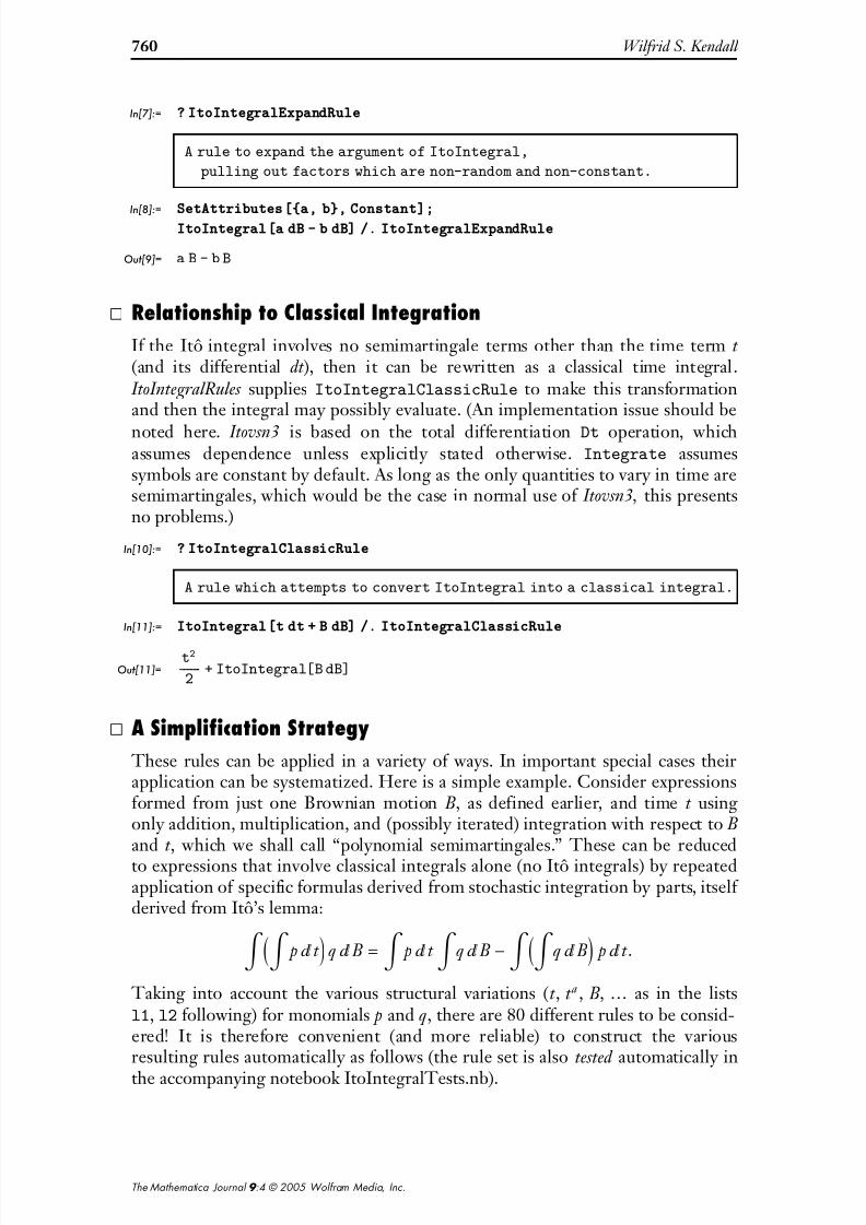
In[7]:= ? ItoIntegralExpandRule

A rule to expand the argument of ItoIntegral,

pulling out factors which are nonrandom and nonconstant.

In[8]:= SetAttributesa, b, Constant;ItoIntegrala dB b dB . ItoIntegralExpandRule

Out[9]= a B b B

· Relationship to Classical Integration

If the Itô integral involves no semimartingale terms other than the time term t (and its differential dt ), then it can be rewritten as a classical time integral.

ItoIntegralRules supplies ItoIntegralClassicRule to make this transformationand then the integral may possibly evaluate. (An implementation issue should be

noted here. Itovsn3 is based on the total differentiation Dt operation, whichassumes dependence unless explicitly stated otherwise. Integrate assumessymbols are constant by default. As long as the only quantities to vary in time aresemimartingales, which would be the case in normal use of Itovsn3, this presentsno problems.)

In[10]:= ? ItoIntegralClassicRule

A rule which attempts to convert ItoIntegral into a classical integral.

In[11]:= ItoIntegralt dt B dB . ItoIntegralClassicRule

Out[11]=t2

2

ItoIntegralB dB

· A Simplification Strategy

These rules can be applied in a variety of ways. In important special cases theirapplication can be systematized. Here is a simple example. Consider expressionsformed from just one Brownian motion B, as defined earlier, and time t usingonly addition, multiplication, and (possibly iterated) integration with respect to Band t , which we shall call “polynomial semimartingales.” These can be reducedto expressions that involve classical integrals alone (no Itô integrals) by repeatedapplication of specific formulas derived from stochastic integration by parts, itself derived from Itô’s lemma:

‡ J‡ p „ t N q „ B = ‡ p „ t ‡ q „ B - ‡ J‡ q „ BN p „ t . Taking into account the various structural variations (t , t a , B, … as in the listsl1, l2 following) for monomials p and q, there are 80 different rules to be consid-ered! It is therefore convenient (and more reliable) to construct the variousresulting rules automatically as follows (the rule set is also tested automatically in

the accompanying notebook ItoIntegralTests.nb).





In[12]:= ItoIntegralRewriteRuleset

Modulea, b, c, d, conv, l1, l2,

SetAttributesa, b, c, d, conv, Constant;

conv Map# ConditionPattern#, Blank, Greater#, 1 &,

a, b, c, d;

l1 t, ta

, B, Bb

, t B, t Bb

, ta

B, ta

Bb

;l2 t, tc , B, Bd , t B, t Bd , tc B, tc

Bd;

Map#1 . conv #2 &, Flatten

MapSolve# ItoIntegraldB ItoIntegralItoD# ItoIntegraldB .

ItoIntegralExpandRule, ItoIntegral# dB &, l1,

MapSolveItoIntegral# dt ItoIntegraldB

ItoIntegralItoDItoIntegral# dt ItoIntegraldB .

ItoIntegralExpandRule,

ItoIntegralItoIntegral# dt dB &, l2,

MapSolveItoIntegral#2 dt ItoIntegral#1 dB

ItoIntegralItoDItoIntegral#2 dtItoIntegral#1 dB . ItoIntegralExpandRule,

ItoIntegralItoIntegral#2 dt #1 dB &,

OuterList, l1, l2, 2

;

The rule set must be applied iteratively to suitable expressions until they stopchanging, so we use FixedPoint to construct an appropriate function. (Note theargument iter, controlling maximum number of iterations, is set by default toInfinity since there is no a priori upper bound on the number of iterationsrequired to simplify a general polynomial semimartingale.)

In[13]:= applyItoRewriteRulesx_, iter_: Infinity :

FixedPoint# . ItoIntegralExpandRule . ItoIntegralRewriteRuleset .

ItoIntegralClassicRule Expand &, x, iter We can test this simplification procedure on a famous result from stochasticcalculus: the family of Hermite polynomials forms a structure that is preservedby Itô integration.

In[14]:= Hk_, x_, t_ : 2 tk2HermiteHk,

x

2 t

Expand;

With this definition, we have

‡ H @n, B, t D „ B = H @n + 1, B, t DÅÅÅÅÅÅÅÅÅÅÅÅÅÅÅÅÅÅÅÅÅÅÅÅÅÅÅÅÅÅÅÅÅÅÅÅÅÅÅÅÅÅÅÅ

2 Hn + 1Land here we test this for the first 10 values of n.





In[15]:= Table

Expand Hn 1, B, t

2 n 1

applyItoRewriteRulesItoIntegralHn, B, t dB,

n, 1, 10Out[15]= True, True, True, True, True, True, True, True, True, True

Variations on this approach can be devised for polynomial semimartingales basedon time t and n independent Brownian motions: see Gaines [9, 10] who appliesthe notion of Lyndon bases for shuffle products on free algebras. Rather thanpursuing this, we now turn to consider expectations of stochastic integrals.

‡

ExpectationItô’s lemma may be employed in computation of expectations of semimartingaleexpressions as follows. If we wish to evaluate @ f H X LD, then we may expand f H X Lusing Itô’s lemma. For well-behaved f (e.g., polynomial functions of Brownianmotion), we may replace the differential „ X in the expectation of the stochasticintegral @ f £ H X L „ X D by its drift „ V to obtain @ f £ H X L „ V D. If the drift iszero (as is the case for Brownian motion), the integral then vanishes; if the drift isdeterministic (e.g., the time process t ), then we may simplify further to obtain

Ÿ @ f £ H X LD„ V . It follows by induction that we can evaluate an expectationcompletely if the semimartingale expression X is a combination of linear opera-

tions, multiplication, and stochastic integration performed on time t and nindependent Brownian motions (what we called a polynomial semimartingale inthe previous section).

ItoIntegralRules therefore defines an expectation operator , which possesses basiclinearity properties, and an associated function , which applies transformationsof the previous form whenever the semimartingale expression is a polynomialsemimartingale.

· Examples

We first consider some simple examples of expectations of polynomial semimart-

ingales. Here is a computation of AHŸ B4„ BL2 E.

In[16]:= ItoIntegralB4 dB2 Out[16]= ItoIntegralB4 dB2

In[17]:= ItoIntegralB4 dB2 .

Out[17]= 21 t5





Higher-order powers can be dealt with in an equally direct manner, though with

increasing computational effort. Here we tabulate @H1 + Ÿ B4„ BLn D for values of

n up to 5.

In[18]:= Table 1 ItoIntegralB4 dBn , n, 1, 5 TableForm

Out[18]//TableForm=

1

1 21 t5

1 63 t5

1 126 t5

2967183 t10

5

1 210 t5 2967183t10

Iterated integrals can be disposed of in a similar fashion. Here we evaluate

AHŸ ‰t Ÿ ‰-t „ B „ t L8 E. Note that can deal with nonpolynomial functions of t .

In[19]:=

ItoIntegraldt

t

ItoIntegraldBt

8

Out[19]=

105 16

3 4 t

2 t

2 t4

Here we evaluate AIŸ HŸ B sinHt L „ t L2„ BM2 E.

In[20]:= ItoIntegralItoIntegralB Sint dt2dB2

Out[20]=3

256

72 t 96 t3 320t Cos2 t 28t Cos4 t

160Sin2 t 128t2 Sin2 t 25 Sin4 t 8 t2 Sin4 t

Nonpolynomial semimartingales are left unsimplified if the nonpolynomial part involves Brownian motions, as in this evaluation of @HB + sinHBLL4 D.

In[21]:= B SinB4Out[21]= 3 t2

4 B3 SinB 6 B2 SinB2 4 B SinB3 SinB4

There are further techniques available for dealing with nonpolynomial semimart-

ingales. For example, consider the evaluation of @sinHBL2 D. We could of courseevaluate this directly using the density for the random variable B, and this itself can be automated using mathStatica [11]. However, we can also make progress

using two further ItoIntegralRules (ItoExpectItoIntegralRule, ItoExpectExÖ

pandRule), which are components of . The first of these implements theinterplay between expectation and drift described at the start of this section,

while the second expands linearly and extracts nonrandom terms.

In[22]:= WithX SinB2,

X . ItoExpectItoIntegralRule . Cosx_2 1 Sinx2 .

ItoIntegralExpandRule . ItoExpectExpandRuleOut[22]= t 2 ItoIntegraldt SinB2

We have thus obtained a recursive expression for

@sin

HB

L2

Dthat can now be used

to form a differential equation by further developing this code.





In[23]:= WithX SinB2,

DSolveDxt, t DX . ItoExpectItoIntegralRule .

Cosx_2 1 Sinx2 . ItoIntegralExpandRule .

ItoExpectExpandRule . X xt .

ItoIntegralClassicRule, t

,

x0 InitialValue0, X, xt, t

Out[23]= xt

1 2

2 t 1

2 t

So we obtain

@sin HBL2 D = 1ÅÅÅÅÅÅ2 H1 - ‰

-2 t L.Further examples can be found in ItoIntegralTests.nb. This differential equationapproach can be applied even when we require the expectation of a quantity that

is not a simple function of Brownian motion. See, for example, the treatment of the distribution of the stochastic area integral Ÿ A„ B - Ÿ B „ A in [2].

· Calculations for the Ornstein–Uhlenbeck Process

The original motivation for this work was to provide an environment to aidcomputations of expectations of quantities associated with the integratedOrnstein–Uhlenbeck process. To illustrate this, we use a pair of stochasticdifferential equations

dU = dB -

a

ÅÅÅÅÅÅ2 U dt

dX = U dt

to define an Ornstein–Uhlenbeck process and its integrated variant. To do thisin Itovsn3 we use Itosde.

In[24]:= SetAttributesΑ, U0, X0, Constant;

ItosdeU, dU dB

Α

2U dt, U0;

ItosdeX, dX U dt, X0;

Note that it must be stated explicitly that botha

and the initial values U 0, X 0are Constant in time. It is possible to solve these linear stochastic differentialequations in closed form: U = ‰

-a t ê2 HU H0L + ‰a t ê2 „ BL and X = X H0L + U „ t .

We express the solutions using ItoIntegral:

In[27]:= UU Α t2 U0 ItoIntegral

Α t2 dBOut[27]=

t Α

2 U0 ItoIntegraldB

t Α 2

and

In[28]:= XX X0 ItoIntegral U dt . U UU

Out[28]= X0 ItoIntegraldt t Α 2 U0 ItoIntegraldB

t Α 2





and verify directly that they satisfy the relevant stochastic differential equations:

In[29]:= ItoDUU dB

Α

2UU dt && InitialValue0, UU U0 Simplify

Out[29]= True

In[30]:= Simplify ItoDXX UU dt && InitialValue0, XX X0 Out[30]= True

We now compute mean values

In[31]:= UUOut[31]=

t Α

2 U0

In[32]:= XX Expand

Out[32]= X0

2 U0

Α

2

t Α 2 U0

Α

and the variance-covariance matrix (using @ X , Y D = @ X , Y D - @ X D @Y D).In[33]:= Outer , B, UU, XX, B, UU, XX MatrixForm

Out[33]//MatrixForm=

t 2

Α

2

t Α

2

Α

4

Α2

4

t Α 2

Α

2 2 t

Α

2

Α

2

t Α

2

Α

1

Α

t Α

Α

2

Α2

2 t Α

Α

2 4

t Α

2

Α

2

4

Α

2 4

t Α

2

Α

2 2 t

Α

2

Α2

2 t Α

Α

2 4

t Α

2

Α

2 12

Α

3 4

t Α

Α

3 16

t Α

2

Α

3 4 t

Α

2

Computation of the fourth central moment is equally direct.

In[34]:= XX XX4

Out[34]=48

2 t Α 1 4 t Α

2 t Α 3 t Α

2

Α6

The image analysis application required the derivation of the conditional distribu -tion of X and U at a specified time s given the values of X and U at 0 and t , for0 < s < t . Since H X , U L is a Gaussian process, we can find this by straightforwarduse of the Statistics‘MultinormalDistribution‘ package once the means

and variance-covariance matrix are calculated for the various values of X and U at times 0, s , and t . Of course it is possible to derive the conditional distribution by hand; an advantage of working in Mathematica is that we are then able to proceeddirectly to simulation experiments and so forth.

‡ Conclusion

We have shown in this article (and in ItoIntegralTests.nb) how the package Itovsn3 can be extended to provide the ability to manipulate stochastic integrals

and compute expectations of stochastic calculus quantities. Further extensionsare possible—we have already noted Gaines’ work [9, 10] on simplification of





polynomial semimartingales based on several independent Brownian motions. A more ambitious extension would be to generalize and automate the differential

equation strategy described here for computing expectations, such as @sinHBL2 D. This would be a demanding project involving the automatic recognition of differential equations satisfied by the expectation in question. We have also

noted the possibility of interaction with other packages such as mathStatica. Forexample, Colin Rose has pointed out how the definition of can be modified soas to invoke mathStatica’s Expect function when the expression has been deter-mined not to be a polynomial semimartingale. This would provide a direct means

of computing @sinHBL2 D; however, differential equation techniques would still berequired when dealing with expressions involving stochastic integrals.

‡ Acknowledgments

This work was supported by EPSRC grant GR/M75785. I am grateful for many helpful discussions with my collaborators on this grant: Abhir Bhalerao, Elke

Thönnes, and Roland Wilson. It is a pleasure to acknowledge the hospitality of David Nualart and the Statistics Department of the University of Barcelonaduring part of the writing process. Thanks are also due to the insightful remarksof two referees, and I am particularly indebted to Colin Rose for his enthusiasticeditorial contributions, which ranged from incisive stylistic advice all the way tosource-code optimization!

Calculations were carried out on a Sun Ultra-10 workstation using Mathe-matica 4.1.

‡ References

[1] W. S. Kendall, “Itovsn3: Doing Stochastic Calculus with Mathematica ,” Economic and Financial Modeling with Mathematica (H. R. Varian, ed.), New York: Springer-Verlag,1993 pp. 214–239.

[2] W. S. Kendall, “Stochastic Calculus in Mathematica: Software and Examples,”University of Warwick Department of Statistics Research Report 333 (Jan 2003)www.warwick.ac.uk/go/wsk/ppt/333.pdf.

[3] B. K. Øksendal, Stochastic Differential Equations , 5th ed., Berlin: Springer Universitext,1998.

[4] A. Bhalerao, E. Thönnes, W. S. Kendall, and R. G. Wilson, “Inferring Vascular Structurefrom 2D and 3D Imagery,” in Medical Image Computing and Computer-Assisted Intervention, Proceedings MICCAI 2001, (W. J. Niessen and M. A. Viergever, eds.),pp. 820–828; Lecture Notes in Computer Science 2208 , Springer, 2001pp. 820–828; University of Warwick Department of Statistics Research Report 392(Jan 2002) www.warwick.ac.uk/go/wsk/ppt/392.pdf.





[5] E. Thönnes, A. Bhalerao, W. S. Kendall, and R. G. Wilson, “A Bayesian Approach toInferring Vascular Tree Structure from 2D Imagery,” in International Conference on

Image Processing , Proceedings ICIP 2002 , (W. J. Niessen and M. A. Viergever, eds.),pp. 937–939; University of Warwick Department of Statistics Research Report 391(Oct 2001) www.warwick.ac.uk/go/wsk/ppt/391.pdf .

[6] J. M. Steele and R. A. Stine, “Mathematica and Diffusions,” Economic and Financial Modeling with Mathematica , (H. R. Varian, ed.), New York: Springer-Verlag, 1993pp. 192–214.

[7] M. Fisher, “ItosLemma.m” MathSource (May20,2002) library.wolfram.com/database/MathSource/1170 (or www.markfisher.net/~mefisher/mma/mathematica.html).

[8] S. Cyganowski, “Solving Stochastic Differential Equations with Maple” Computer Algebra: Maple Tech, 3(2), 1986 pp. 35–40.

[9] J. G. Gaines, “The Algebra of Iterated Stochastic Integrals,” Stochastics and Stochastics Reports, 49(3–4), 1994 pp. 169–179.

[10] J. G. Gaines, “A Basis for Iterated Stochastic Integrals,” Mathematics and Computers in

Simulation [online], 38(1–3), 1995 pp. 7–11.dx.doi.org/10.1016/0378-4754(93)E0061-9.

[11] C. Rose and M. D. Smith, Mathematical Statistics with Mathematica , Springer Texts inStatistics, New York: Springer-Verlag, 2002.

‡ Additional Material

Itovsn3.zip (zip archive containing the files init.m, ItoIntegralRules.m, andItoIntegralTests.nb).

Available at www.mathematica-journal.com/issue/v9i4/download.

About the Author

Wilfrid S. Kendall is a professor of statistics at the University of Warwick, with variedresearch interests primarily concerning the way computing and geometry influenceprobability and statistics.

Wilfrid S. Kendall

Department of Statistics University of Warwick Coventry CV4 7AL, UK [email protected] www.warwick.ac.uk/go/wsk



Documents

s to Chas Tic Integrals