158

Volatility Smile/Smirk Properties of [GLP & MEMMM] Models

Yoshio Miyahara’ and Naruhiko MoriwakiGraduate School of Economics

Nagoya City University

Abstract

The [GLP(Geometric Levy Process) & MEMM(Minimal Entropy Martingale Measure)]pricing model was first introduced in [13] as one of the pricing models for the incompletemarket. We first explain the structure of this model, and next we investigate the volatility$\mathrm{s}\mathrm{m}\mathrm{i}\mathrm{l}\mathrm{e}/\mathrm{s}\Pi \mathrm{u}\mathrm{r}\mathrm{k}$ properties of this model by the use of computer simulation method.

1 Introduction

It is well-known that the implied volatility surface has smile or smirk properties in the realmarkets, and this property is called volatility $\mathrm{s}\mathrm{m}\mathrm{i}\mathrm{l}\mathrm{e}/\mathrm{s}\mathrm{m}\mathrm{i}\mathrm{r}\mathrm{k}$ property (or $\mathrm{s}\mathrm{m}\mathrm{i}\mathrm{l}\mathrm{e}/\mathrm{s}\mathrm{k}\mathrm{e}\mathrm{w}$ property).This fact suggests us that the construction of a new option pricing model, which possesses thissm $\mathrm{i}\mathrm{l}\mathrm{e}/\mathrm{s}\mathrm{m}\mathrm{i}\mathrm{r}\mathrm{k}$ property, is inevitable.

Several kinds of models have been proposed and investigated. The [GLP & MEMM ] pricingmodel is one of them, and it is known that this model have many good properties as an optionpricing model for the incomplete market. (See $[13|$ and $[15|$ ). In this paper we investigate thevolatility $\mathrm{s}\mathrm{m}\mathrm{i}\mathrm{l}\mathrm{e}/\mathrm{s}\mathrm{m}\mathrm{i}\mathrm{r}\mathrm{k}$ properties of the [GLP & MEMM] pricing models by the use of computersimulation method.

In $\S\underline{7}$ we survey the volatility $\mathrm{s}\mathrm{m}\mathrm{i}\mathrm{l}\mathrm{e}/\mathrm{s}\mathrm{m}\mathrm{i}\mathrm{r}\mathrm{k}$ proble$\mathrm{m}\mathrm{s}$ . In \S 3 we explain the [GLP& MEMM]model briefly and in \S 4 vxe give several examples of it. In \S 5 we see that the [GLP & MEMM]model possesses the volatility $\mathrm{s}\mathrm{m}\mathrm{i}\mathrm{l}\mathrm{e}/\mathrm{s}\mathrm{m}\mathrm{i}\mathrm{r}\mathrm{k}$ properties in various forms. Finally in 56 we discussthe calibration results of of Nikkei 225 options by the [GLP & MEMM] models.

Tlle results obtained in this paper show us that the [GLP & MEMM] model is a very strongcandidate for the llew model wliich should have the volatility $\mathrm{s}\mathrm{m}\mathrm{i}\mathrm{l}\mathrm{e}/\mathrm{s}$ mirk property and thatthis model can be applied to the calibration problems.

Corresponding author. $\mathrm{E}$-mail: y-miya@econ.nagoya-cu ac.jp

数理解析研究所講究録 1462巻 2006年 156-170

157

2 Volatility $\mathrm{S}\mathrm{m}\mathrm{i}\mathrm{l}\mathrm{e}/\mathrm{S}$mirk Problems

2.1 Historical Volatility and Implied Volatility for Black-Scholes Model

The Black-Scholes model is the special case of GLP model with no jump part, namely the process

is given by$S_{t}=S_{0}e^{(\mu-\frac{1}{2}\sigma^{2})t+\sigma W_{t}}$ , (2.1)

or in the form of stochastic differential equation

$dS_{t}=S_{\mathrm{t}}(\mu dt+\sigma dWt)$ , (2.2)

where $\mu$ is called the drift parameter and a is called the volatility parameter.

The theoretical B-S price of the European call option $C_{K}$ with the strike price $K$ and the

fixed maturity $T$ is given by the following formula

$C_{K}=S\mathrm{o}\Phi(d_{1})-e^{-rT}K\Phi(d_{2}))$ (2.3)

where $\Phi(d)$ is the normal distribution function and

$d_{1}= \frac{\log\not\simeq s+(r+\frac{\sigma^{\vee}}{2})T}{\sigma\sqrt{T}},1$ $d_{2}= \frac{\log\frac{S0}{K}+(r-\frac{\sigma^{2}}{2})T}{\sigma\sqrt{T}}=d_{1}-\sigma\sqrt{T}$ (2.4)

Under the above setting, the historical volatility of the process is the estimated value of a

based on the sequential data of the price process $S_{t}$ . We denote it by $\hat{\sigma}$ . On the other hand the

implied volatility is defined as what follows. Suppose that the market price of the European call

option with the str\$\cdot$

&e $K$ , say $C_{K}^{(m\}}$ , were given. Then the value of a which satisfies the following

equation$S_{0}\Phi(d_{1})-e^{-rT}K\Phi(d_{2})=C_{K}^{(m)}$ , (2.5)

is the implied volatility, and this value is denoted by $\sigma_{K}^{(im\rangle}$ . We remark here that the implied

volatitity $\sigma_{K}^{(im)}$ depends on the strike value $K$ , and on the contrary the historical volatility $\hat{\sigma}$

does not depend on $K$ .

2.2 Volatility $\mathrm{S}\mathrm{m}\mathrm{i}\mathrm{l}\mathrm{e}/\mathrm{S}\mathrm{m}\mathrm{i}\mathrm{r}\mathrm{k}$ Properties of Market Option Prices

We first consider the case where the market value of options obey to the Black-Scholes model, and

so the market price $C_{h’}^{(m\}}$ is equal to the theoretical B-S price $C\kappa$ of (2.3). In this case the solution

of the equation $(2,5)$ is equal to the original a and it holds true that $\sigma_{K}^{(im)}=\sigma=constant$ . This

means th at if the market obeys exactly to the Black-Scholes model, then the implied volatility

$\sigma_{K}^{(in\iota)}$ should be equal to the historical volatility $\hat{\sigma}(=\sigma)$ .

But in the real world this is not true. It is well-known that the implied volatility is not equal

to the historical volatility, and the implied volatility curve $\sigma_{K}^{(im)}$ is sometimes a convex function

of $K$ , and sometimes the combination of convex part and concave part, These properties are

so-called volatility sm ile or smirk properties.

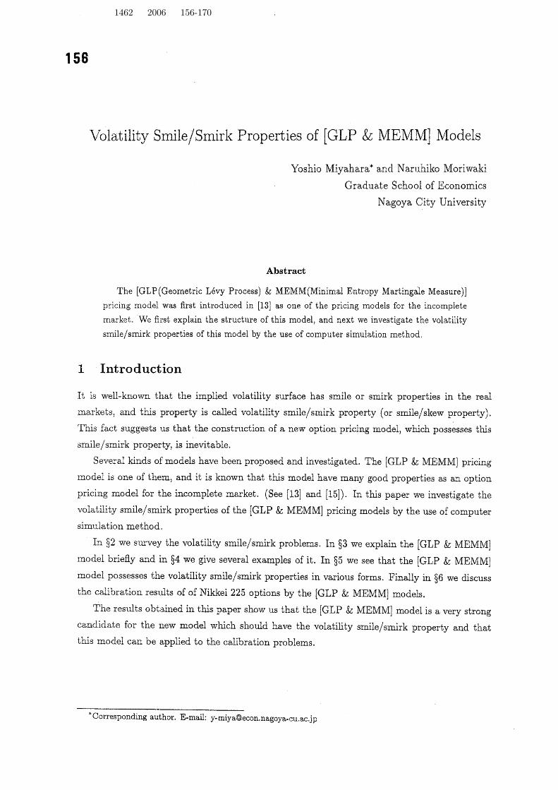
The Figure 1, 2, 3, and Table 1, 2 illustrate this situation, where a new variable moneyness

$(= \frac{\mathrm{A}’}{s_{0}})$ is introduced

158

Figure 1: Implied volatility surface for Nikkei 225 index options. (July-2002, time to maturity

is 20-day or more)

Figure 2: 07/02/2001, time to maturity $=30-$ Figure 3: 18/01/2000, time to maturity $=52arrow$

day, volatility $\mathrm{S}\mathrm{l}\mathrm{n}\mathrm{i}\mathrm{l}‘ \mathrm{d}$} day, volatility smir

158

Table 1: Historical Volatility vs Implied Volatility

To consider the volatility $\mathrm{s}\mathrm{m}\mathrm{i}\mathrm{l}\mathrm{e}/\mathrm{s}\mathrm{m}\mathrm{i}\mathrm{r}\mathrm{k}$ properties of market option prices, we use the data of

Nikkei 225 call options traded at OSE (Osaka Stock Exchange), whose time to maturity is less

than or equal to 40-days and whose trading volume is more than 50. In this case, we have

obtained such a result that the Nikkei 225 call option has the volatility smile property for each

year.

err ratio: mean during 1-year of (implied volatility - historical volatility) / historical volatility.

Tlle historical volatility is estimated from the $\log$ returns of recent 245 days.

Table 2: Historical Volatility vs Implied Volatility

To consider the volatility $\mathrm{s}\mathrm{m}\mathrm{i}\mathrm{l}\mathrm{e}/\mathrm{s}\mathrm{m}\mathrm{i}\mathrm{r}\mathrm{k}$ properties of market option prices, we use the data of

Nikkei 225 call options traded at OSE (Osaka Stock Exchange), whose time to maturity is more

than 40-days and whose trading volu me is more than 50. In this case, we have obt ined such a

$1^{\backslash }\mathrm{e}\mathrm{s}\iota \mathrm{d}\mathrm{t}$ that the Nikkei 225 call option has the volatility sm irk property for each year.

err ratio: mean during 1-year of (implied volatility $arrow$ historical volatility) / historical volatility.

The historical volatility is estimated from the $1o\mathrm{g}$ returns of recent 245 days.

180

2.3 Volatility $\mathrm{S}\mathrm{m}\mathrm{i}\mathrm{l}\mathrm{e}/\mathrm{S}\mathrm{m}\mathrm{i}\mathrm{r}\mathrm{k}$ Properties of Models

Based on the above facts, new models, which have the volatility $\mathrm{s}\mathrm{m}\mathrm{i}\mathrm{l}\mathrm{e}/\mathrm{s}\mathrm{m}\mathrm{i}\mathrm{r}\mathrm{k}$ property, are

required. A pricing model is said to have the volatility smile property or volatility smirk property

if the implied volatility function for the theoretical option prices of that model has the volatility

smile or smirk property. Let $C_{K}^{*}$ be the theoretical option price of the new model and let $\sigma_{K}^{(7m)*}$

be the solution of$S0\Phi(d_{1})-e^{-rT}K\Phi(d2)=C_{I\zeta}^{*}$ . (2.6)

Then $\sigma_{K}^{\langle im)*}$ is the implied volatility related to the new model. If $\sigma_{K}^{(im)*}$ has the volatility smile

property, then the model is said to have the volatility smile property, and if $\sigma_{K}^{(im)*}$ has the

volatility smirk property, then the model is said to have the volatility smirk property.

3 [GLP & MEMM] Pricing Model

The [GLP & MEMM] Pricing Model is such a model:(A) The price process $S_{t}$ is a geometric L\’evy process (GLP).

(B) The price of an option $X$ is defined by $e^{-rT}E_{P}*[X]$ , where $P^{*}$ is the minimal entropy

martingale measure (MEMM).$\mathrm{T}\mathrm{l}\dot{\mathrm{u}}\mathrm{s}$ model was first introduced in [13], and the properties of $\mathrm{t}\mathrm{l}\dot{\mathrm{u}}\mathrm{s}$ model are sum marised in

[15].

3.1 Geometric Levy Process (GLP)

The price process $S_{t}$ of a stock is assumed to be defined as what follows. We suppose that a

probability space $(\Omega, F, P)$ and a filtration $\{F_{t}, 0\geq t\geq T\}$ are given, and that the price process$S_{t}=S_{0}e^{Z_{t}}$ of a stock is defined on this probability space and given in the form

$S_{t}=S0e^{Z_{\mathrm{t}}}$ , $0\leq t\leq T$ , (3.1)

where $Z_{t}$ is a L\’evy process. We call such a process $S_{t}$ the geometric Levy precess (GLP), andwe denote the generating triplet of $Z_{t}$ by $(\sigma_{Z}^{2}, l\nearrow z(dx)$ , $b_{Z})$ or simply by $(\sigma^{2}, \iota/(dx),$ $b)$ .

3.2 Minimal Entropy Martingale Measure (MEMM)

We first give the definition of the MEMM.

Definition 1 (minimal entropy martingale measure (MEMM)) If an equivalent martin-gale measure $P^{*}$ satisfies

$H(P^{*}|P)\leq H(Q|P)$ $\forall Q$ : equivalent martingale measure, (3.2

181

then $P^{*}$ is called the minimal entropy martingale measure (MEMM) of $S_{t}$ . Where $H(Q|P)$ is

the relative entropy of $Q$ with respect to $P$

$H(Q|P)= \{\int_{\infty}\Omega,\log \mathrm{f}[_{\mathrm{f}}^{dQ}|dQ,$ $otherw\mathrm{i}see\mathrm{i}fQ<<,P$

,$\}$ , (3.4)

3.3 Sufficient Conditions for the Existence of the MEMM

The existence problem of the MEMM of geometric L\’evy processes has been studies in [12], [3]

and [13], and finally those results are generalized in [7] as the following form.

Theorem 1 (Pujiwara-Miyahara [7, Theorem 3.1]) Suppose that the following condition

(C) holds

Condition (C) There exists $\theta^{*}\in R$ which satisfies the following conditions :

$(\mathrm{C})_{1}$ $\int_{\{x>1\}}e^{x}e^{\theta\langle e^{\varpi}-1)}.\iota/(dx)<\infty$ , (3.4)

$(\mathrm{C})_{2}$ $b+( \frac{1}{2}+\theta^{*})\sigma^{2}+\int_{\{|x|>1\}}(e^{x}-1)e^{\theta(e^{x}-1)}.\nu(dx)$

$+f_{\{|x|\leq 1\}}((e^{x}-1)e^{\theta^{*}(e^{x}-1)}-x)\nu(dx)$ $=r$ . (3.5)

Then the probability measure $P^{*}$ is well defined and it holds that

(i)(MEMM): $P^{*}$ is the MEMM of $S_{t}$ .(ii) (L\’evy process): $Z_{t}$ is also a L\’evy process $w.r.t$ . $P^{*}$ , and the generating triplet (A* , $\nu^{*}$ , $b^{*}$ ) of$Z_{t}$ under $P^{*}$ is

A$*$

$=$$\sigma^{2}$ , (3.6)

$l^{f^{*}}(dx)$ $=$ $e^{\theta^{\wedge}(e^{oe}-1)}\nu(dx)$ , (3.7)

$b^{*}$ $=$ $b+ \theta^{*}\sigma^{2}+\int_{R\backslash \{0\}}xI_{\{|x|\leq 1\}}d(\nu^{*}-\iota/)$ . (3.8)

3.4 Prices of European Call Options

We investigate the European call option. The price of European call option is

$C(S_{0}, K, T)=e^{-rT}E_{P}$ . $[(S_{T}-K)^{+}]$ . (3.9)

It is known that this value is computed as follows.

The characteristic function $\phi_{\mathrm{t}}^{*}(u)$ of $Z_{t}$ under the MEMM $P^{*}$ is

$\phi_{\mathrm{t}}^{*}(u)=\phi_{Z_{l}}^{*}(u)=E_{P^{*}}[\mathrm{e}^{i\mathrm{u}Z_{\mathrm{t}}}]=\exp(\psi_{t}^{*}(u))=\exp(t\psi^{*}(u))$ , $i=\sqrt{-1}$ , (3.10)

where $\psi^{*}(u)=\psi_{1}^{*}(u)$ .

Set$\zeta(v;S_{0}, T)=S_{0}\frac{e^{-rT}\phi_{T}^{*}(v-\mathrm{i})-e^{ivrT}}{\mathrm{i}v(1+iv)}$ $(3.11\rangle$

182

and$\tilde{c}(k\cdot S_{0}, T)|=\frac{1}{2\pi}\int_{-\infty}^{\infty}e^{-ikv}\zeta(v;S_{0}, T)dv$ (3.12)

Then the price of the European call option $C(S_{0}, K, T)$ is com puted as

$C$ (So, $K,$ $T$) $=\tilde{c}(\log(K/S\mathrm{o});S_{0},T)+(S_{0}-e^{-rT}K)^{+}$ . (3.13)

(See [15].) $\mathrm{T}\mathrm{l}\dot{\mathrm{u}}\mathrm{s}$ method is used in \S 5 for the computation of the theoretical option prices.

4 Examples of [GLP & MEM M] Pricing Model

In this section we see several examples of [GLP &MEMM] Pricing Models. To do this, we have

to check the existence of the MEMM, i.e. we have to examine that the given geometric L\’evy

process $S_{t}=S0\exp Z_{i}$ satisfies the Condition (C). Set

$f(\theta)$ $=$ $b+( \frac{1}{2}+\theta)\sigma^{2}+\int_{\langle|x|>1\}}(e^{x}-1)e^{\theta(e^{\mathfrak{B}}-1)}\nu(dx\}$

$+l_{|x|\leq 1\}}((e^{x}-1)e^{\theta(e^{x}-1)}-x)\mathrm{u}(\mathrm{d}\mathrm{x})$ . (4.1)

Then the condition $(\mathrm{C})_{2}$ is equivalent to that $\theta^{*}$ is the solution of

$f(\theta)=r$. (4.2)

4.1 [Geometric Stable Process & MEMM] Model

We consider tlle stable model. Suppose that $Z_{t}$ is a stable process and let $(0 \nu(\}dx), b)$ be its

generating triplet. The L\’evy measure is

$\nu(dx)=c_{1}I\{x<0\}|x|^{-(\alpha+1)}dx+\mathrm{c}_{2}I\{x>0\}|x|^{-(\alpha+1)}dx$ , (4.3)

where $0<$ a $<2$ and we assume that

$c_{1}>0$ , $c_{2}>0$ . (4.4)

It is shown that the equation (4.2) has a unique solution $\theta^{*}$ and that 0’ is negative. (See [7]

or [16].) So the geometric stable process model is an exam ple of the [GLP & MEMM] Pricing

Model.

4.2 [Geometric CGMY Process & MEM M] Model

The Levy measure of the CGMY process is

$\mathrm{v}\{\mathrm{d}\mathrm{x}$ ) $=C(I\{x’<0\}\exp(-G|x|)+I\{x>0\}\exp(-M|x|))|x|^{-(1+Y)}dx$ , (4.5)

where $C>0$ , $G\geq 0$ , $M\geq 0$ , $Y<2$ (see [1]). If $Y\leq 0$ , then $G>0$ and $M>0$ are assu med.We mention 1ere that the case $Y=0$ is the VG process case, and the case $G=M=0$ and$0<Y<2$ is the symmetric stable process case. In the sequel we assume that $G$ , $M>0$ .

For this model the following results are obtained (see [16])

163

Proposition 1 (1) If $M\leq 1$ , then the equation $f(\theta)=r$ has a unique solution $\theta_{\mathrm{J}}^{*}$ and the

solution is negative,

(2) If $M>1$ and $f(0)\geq r$ , then the equation $f(\theta)=r$ has a unique solution $\theta^{*}$ , and the solution

is $nonarrow pos\mathrm{i}t\mathrm{i}ve$.(3) If $M>1$ and $f(0)<r$ , then the equation $f(\theta)=r$ has $na$ solution.

4.3 [(Qeometric Variance Gamma Process & MEMM] Model

The Levy measure of Variance Gam ma process is of the following form (see [8]).

$\nu(dx)=C(I_{\{x<0\}\mathrm{P}(-c_{1}|x|1+I_{\{x>0\}}\exp(-c_{2}|x|))|x|^{-1}dx},$ (4.6)

where $C$, $c_{1}$ , $c2$ are positive constants.

The following results are obtained (see[7] or [16]).

Proposition 2 (1) if $c2\leq 1$ , then the equation $f(\theta)=r$ has a unique solution 2*, and the

solution is negative,

(2) If $c2>1$ and $f(0)\geq r$ , then the equation $f(\theta)=r$ has a unique solution $\theta^{*}$ , and the solution

$\dot{\mathrm{z}}s$ non-positive.

(3) If. $c_{2}>1$ and $f(0)<r_{f}$ then the equation $f(\theta)=r$ has $na$ solution.

5 Volatility Sm\’ile/Smirk Properties of [GLP & MEMM] $\mathrm{M}\mathrm{o}\mathrm{d}\sim$

els: Simulation Results.

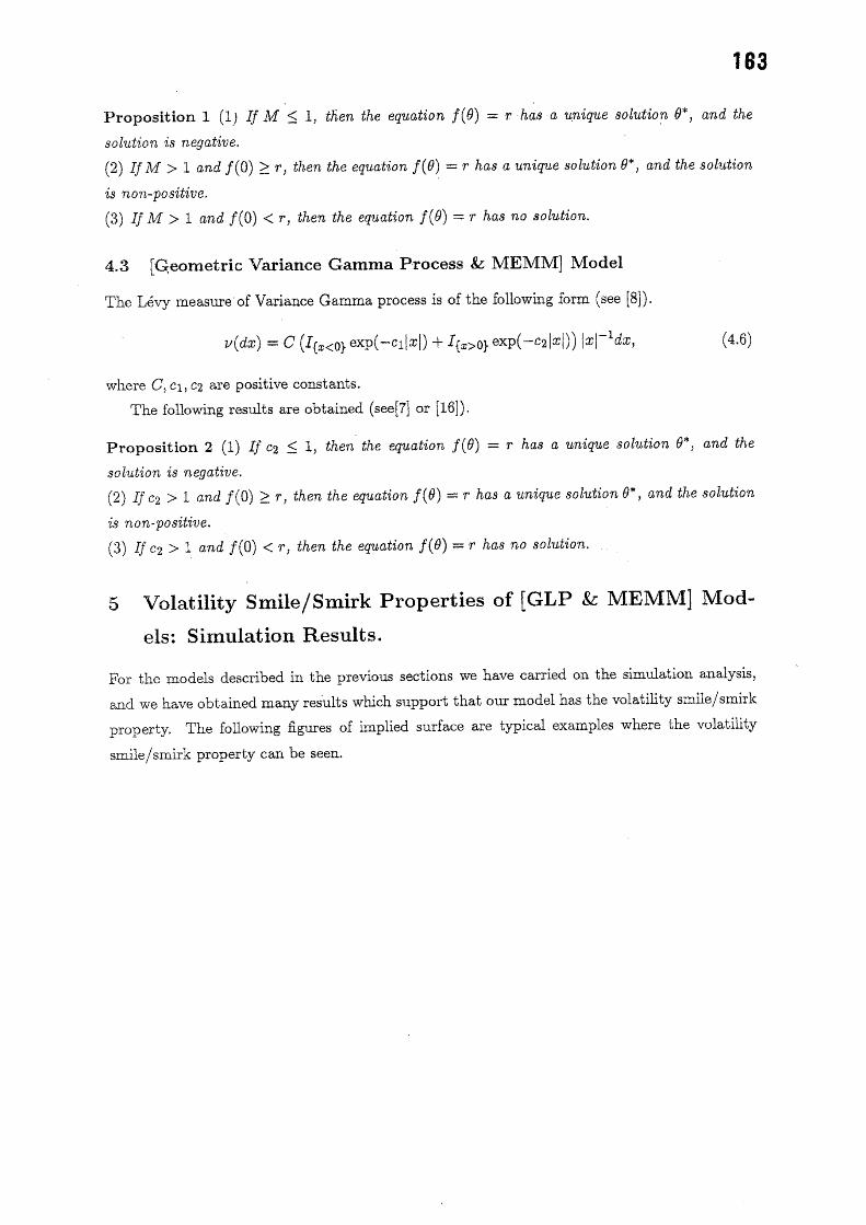
For thle models describ ed in the previous sections we have carried on the simulation analysis,

arzd we have obtained many results which support that our model has the volatility $\mathrm{s}\mathrm{m}\mathrm{i}\mathrm{l}\mathrm{e}/\mathrm{s}\mathrm{m}\mathrm{i}\mathrm{r}\mathrm{k}$

property. The folowing figures of implied surface are typical examples where the volatility

$\mathrm{s}\mathrm{m}\mathrm{i}\mathrm{l}\mathrm{e}/\mathrm{s}\mathrm{m}\mathrm{i}\mathrm{r}\mathrm{k}$ property can be seen

184

5.1 [Geometric Stable Process & MEMM] Model

(a) $b$ $=-0,4$ (b) $b$ $=0$ (c) $b$ $=0.6$

Figure 4. [ $\mathrm{G}$ Stable Process & MEMM] Model $(\alpha=1,2, c_{1}=0.2, c_{2}=0.2)$

(a) $\alpha=0.8$ (b) $\alpha=1.4$ (c) a $=1.8$

Figure 5: [ $\mathrm{G}$-Stable Process & MEMM] Model $(b=0, c_{1}=0.01, c_{2}=0.01)$

(a) $c_{1}=0.005$ , $c2=$ 0.095 (b) $c_{1}=0.095$ , $c_{2}=$ 0.005 (c) $c_{1}=0.2$ , $\mathrm{c}_{2}=0.1$

Figure 6: [ $\mathrm{G}$ Stable Process &MEMM] Model ( $b=0$ , a $=0.2$)

185

5.2 [Geometric CGMY Process & MEMM] Model

(a) $b=-\mathrm{O}.1$ (b) $b=0$ (c) $b=0.2$

Figure 7: [ $\mathrm{G}$-CGMY Process & MEMM] Model $(C=0.05_{\mathrm{I}}G=0.5, M=0.5, Y=1.2)$

(a) $C=0.05$ (b) $C=0.1$ (c) $C=0.3$

Figure 8: CGMY Process & MEMM] Model $(b=0, G=0.5, M=0.5, Y=1.2)$

(a) $G=5$ , $M=0.05$ (b) $G=0.05$ , $M=0.05$ (c) $G=0.05$ , $M=3$

Figure 9: [ $\mathrm{G}$ CGMY Process & MEMM] Model $(b=0, C=0.05, Y=1.2)$

188

(a) $Y=0.5$ (b) $Y=1$ $\langle \mathrm{c}\rangle Y=1.5$

Figure 10: [ $\mathrm{G}$-CGMY Process & MEM $\mathrm{M}$] Model $(b=0, C=0.05, G=0.5, M=0.5)$

5.3 [Geometric Variance Gamma Process & MEMM] Model

(a) $b0=-0.4$ (b) $b0$ $=0$ (c) $b\mathit{0}=0.6$

Figure 11: [G-VG Process & MEM $\mathrm{M}$] Model $(C=5c_{1}=15, c_{2}=0.5\})$

(a) $C=5$ (b) $C=10$ (c) $C=20$

Figure 12: [G-VG Process & MEMMI Model ($b0=0$ , $c_{1}=$ L5, $c_{2}=15$ )

1137

(a) $\mathrm{c}_{1}=15$ , $c_{2}=15$ (b) $c_{1}=28$ , c2 $=2$ (c) $c_{1}=10$ , $c_{2}=10$

Figure 13: [G-VG Process & MEMM] Model $(b0=0, C=10)$

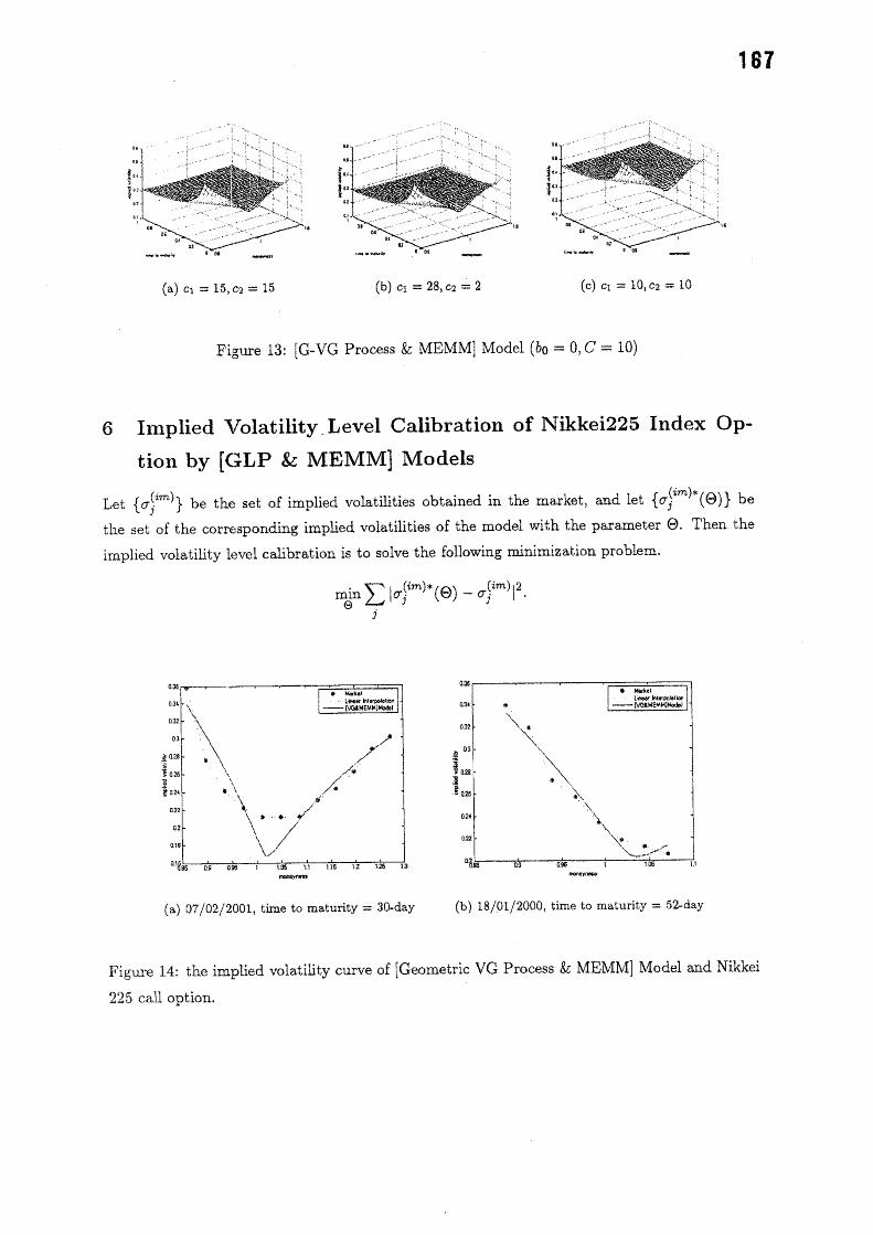
6 Implied Volatility Level Calibration of Nikkei225 Index Op-

tion by [GLP & MEMM] Models

Let $\{\sigma_{j}^{(im)}\}$ be the set of implied volatilities obtained in the market, and let $\{\sigma_{\mathrm{i}}^{(\mathrm{i}m)*}(\Theta)\}$ be

tlle set of the corresponding implied volatilities of the model with the parameter $\Theta$ . Then the

implied volatility level calibration is to solve the following inimization problem.

$\min_{\Theta}\sum_{\mathrm{j}}|\sigma_{j}^{(\mathrm{i}m)*}(\Theta)-\sigma_{j}^{(im)}|^{2}$.

(a) 07/02/2001, time to maturity $=$ $30$ day (b) 18/01/2000, time to maturity $=52$-day

Figure 14: the implied volatility curve of [Geom etric VG Process & MEMM] Model and Nikkei

225 call option

168

(a) 07/02/2001, time to maturity $=$ $30$ day (b) 18/01/2000, time to maturity $=$ 52-day

Figure 15: the implied volatility curve of [Geometric CGMY Process & MEMM] Model and

Nikkei 225 call option,

(a) 07/02/2001, time to maturity $=$ $30$ day (b) 18/01/2000, time to maturity $=$ 52-day

Figure 16: the implied volatility curve of [Geometric Stable Process & MEMM] Model andNikkei 225 call option,

189

7 Concludin${ }$ Remarks

We have only done the implied volatility level calibration. For the selection of $\mathrm{s}$ uitable model,

we have to do the option price level calibration and the fitness analysis. These analyses are the

subjects for us to do next.

References

[1] Carr, P., Gem an} H., Madan, D.B., and Yor, M. (2000), The Fine Structure of Asset

Returns: An Empirical Investigation. (Preprint),

[2] Carr, P. and Madan, D. (1999), Option valuation using the fast Fourier transform. Journal

of Computational Finance, 2, 61-73.

[3] Chan, T. (1999), Pricing Contingent Claims on Stocks Derived by Levy Processes, The

Annals of Applied Probability, v. 9, No. 2, 504 528 .

[4] Cont, R. and Tankov, P. (2002), Calibration of $\mathrm{J}\iota \mathrm{u}\mathrm{n}\mathrm{p}$-Diffusion Option-Pricing Models: A

Robust Non-parametric Approach, (preprint).

[5] Fama, E. F. (1963), Mandelb rot and the Stable Paretian Hypothesis, J. of Business, 36,

420-429.

[6] Frittelli, M. (2000), The Minim al Entropy Martingale Measures and the Valuation Problem

in Incomplete Markets, Mathematical Finance 10, 39-52,

[7] Fujiwara, T. and Miyahara, Y. (2003), The Minimal Entropy Martingale Measures for

Geometric L\’e\’y Processes, Finance and Stochastics $7(2003)$ , pp.509-531.

[8] Madan, D. and Seneta, E. (1990), The variance gamma (vg) model for share market returns.

Joumal of Business, v.63(4), 511-524.

[9] Madan, D., Carr, P. and Chang, E. (1998), The variance gamma process and option pricing.

European Finance Review, v.2, 79-105.

[10] Mandelbrot, B. (1963), The variation of certain speculative prices. J. of Busin ess, 36,

394-419.

[11] Miyahara, Y.(1996), Canonical Martingale Measures of Incomplete Assets Markets, in Prob-

ability Theory and Mathematical Statistics: Proceedings of the Seventh Japan-Russia Syrn-

posium, Tokyo 1995 (eds. S. Watanabe et al.), pp.343-352.

[12] Miyahara, Y. (1999), Minimal Entropy Martingale Measures of Jump Type Price Processesin Incomplete Assets Markets. Asian-Pacfic Financial Markets, Vol. 6, No, 2, pp. 97-113

170

[13] Miyahara, Y.(2001), [Geometric Levy Process & MEMM] Pricing Model and Related Esti-

mation Problems, Asia-Pacific Financial Markets 8, No. 1, pp. 45-60,

[14] Miyahara, Y.(200 |), Estimation of Levy Processes, Discussion Papers in Economics,

Nagoya City University No, 318, pp. 1-36.

[15] Miyahara, Y.(2004), [GLP & MEMM] Pricing Model and its Calibration, (preprint).

[16] Miyahara, Y. and Novikov, A. (2002), Geometric Levy Process Pricing Model, Proceedings

of Steklov Mathematical Institute, Vo1.237(2002), pp. $176\sim 191$ .

[17] Rachev, S. and Mittnik, S. (2000), ”Stable Paretian Models in Finance” , Wiley.

[18] Sato, K. (1999), “Levy Processes and Infinitely Divisible Distributions”, Cambridge Uni-versity Press