Embed Size (px)
Citation preview

Edited by
Gerhard Bohrmann and Silke Schenck
with contributions of cruise participants
IFM-GEOMAR Leibniz-Institut für Meereswissenschaften an der Universität Kiel
KIEL 2004
GEOMAR REPORT 117
IFM-GEOMAR Leibniz Institute of Marine Sciences at Kiel University
RV SONNE
CRUISE REPORT SO 174
OTEGA II: LOTUS OMEGA MUMM
Investigations within the BMBF special program
"Gashydrate im Geosystem"
BALBOA - CORPUS CHRISTI – MIAMI
1 October – 12 November 2003
Leg SO 174-1: Balboa (Panama) – Corpus Christi (USA)
1 – 24 October 2003
Leg So 174-2: Corpus Christi (USA) – Miami (USA)
25 October – 12 November 2003

Redaktion dieses Reports: Gerhard Bohrmann und Silke Schenck
Editors of this issue: Gerhard Bohrmann and Silke Schenck
GEOMAR REPORT ISSN 0936-5788
GEOMAR REPORT ISSN 0936-5788
Leibniz-Institut für Meereswissenschaften an der Universität Kiel Wischhofstr. 1-3 D - 24148 Kiel Tel. (0431) 600-2555, 600-2505
Leibniz Institute of Marine Sciences at Kiel University Wischhofstr. 1-3 D - 24148 Kiel Tel. (49) 431 / 600-2555, 600-2505

TABLE OF CONTENTS
Preface .................................................................................................................................. 3 Personnel aboard R/V SONNE during cruise SO 174 .......................................................... 7 Participating institutions ....................................................................................................... 9 1. Introduction........................................................................................................................... 10 1.1 Objectives.............................................................................................................................. 10 1.2 The Gulf of Mexico – an overview ....................................................................................... 11 1.3 Gas hydrate in the Gulf of Mexico........................................................................................ 14 2. Cruise narrative ..................................................................................................................... 17 3. Sea floor mapping ................................................................................................................. 25 3.1 Multibeam swathmapping in the northern Gulf of Mexico................................................... 25 3.2 Sub-bottom profiling and plume imaging ............................................................................. 27 3.3 Multibeam echosounding and PARASOUND on the Sigsbee and Campeche Knolls .................................................................................................................................... 34 3.4 Visual seafloor observation................................................................................................... 40 4. Water column program ......................................................................................................... 51 5. Lander deployments .............................................................................................................. 55 5.1 Concept and objectives of the lander program...................................................................... 55 5.2 Biogeochemical Observatory, Fluid Flux Observatory and Bottom Water Sampler ................................................................................................................................. 56 5.3 Deep-sea Observation System (DOS) ................................................................................... 63 5.4 GasQuant............................................................................................................................... 64 5.5 HDSD lander......................................................................................................................... 66 6. Sediment sampling and sedimentology................................................................................. 74 6.1 Geological sampling equipment............................................................................................ 74 6.2 Autoclave tools ..................................................................................................................... 76 6.3 Sedimentological results ....................................................................................................... 80 6.4 Gas hydrate and CT scanning ............................................................................................... 84 6.5 Authigenic carbonates........................................................................................................... 87 7. Pore water and gas investigations ......................................................................................... 89 7.1 Pore water chemistry............................................................................................................. 89 7.2 Gas analysis from sediment cores ......................................................................................... 97 8. Microbial ecology ................................................................................................................. 103 8.1 Leg 1 ..................................................................................................................................... 103 8.2 Leg 2 ..................................................................................................................................... 104 9. Biological sampling .............................................................................................................. 109 9.1 Samples collected.................................................................................................................. 109 9.2 Laboratory activities ............................................................................................................. 110 References............................................................................................................................. 112 Appendix .....................................................................................................................117


R/V SONNE cruise report SO 174/ OTEGA II Preface
3
PREFACE
Gerhard Bohrmann Starting her journey from Balboa, Panama on 6 October, R/V SONNE was scheduled for interdisciplinary work in the Gulf of Mexico (GOM) on near-surface methane hydrate (SO 174, OTEGA-II). During the first leg the ship operated in the northern GOM along the continental slope of Texas in several lease blocks of the Green Canyon Area (Figs.1 and 3). After a mid-leg stop in the harbour of Corpus Christi (24-26 October) the research vessel worked for the first time in southern GOM, in Mexican waters, in the areas of the Sigsbee Knolls, northern Campeche Knolls and on the Yucatan shelf (Figs. 1 and 4). Additional sampling work in some areas of the Green Canyon completed the scientific program in the northern Gulf. The research cruise ended on 11 November in the harbour of Miami (Figure 1).
Fig. 1: Cruise track of R/V SONNE during SO 174 (OTEGA-II). The main program had been set up by the three cooperative projects LOTUS, OMEGA and MUMM, which are funded by the German Federal Ministery of Education and Science (Bundesministerium für Bildung und Forschung, BMBF) within the scope of its special program "Gashydrate im Geosystem" (gas hydrate in the geosystem).

R/V SONNE cruise report SO 174/ OTEGA II Preface
4
- OMEGA: Shallow marine gas hydrates: Dynamics of a sensitive methane reservoir
(http://www.gashydrate.de/projekte/omega/index.html) - LOTUS: Long-term observatory for the study of control mechanisms of the formation
and destabilisation of gas hydrate (http://www.geomar.de/~jgreiner/web_LOTUS/index. html)
- MUMM: Methane in gas-hydrate-bearing marine sediments –Turnover rates and microorganisms (http://www.mpi-bremen.de/deutsch/biogeo/mumm2.html)
Fig. 2: Images taken during cruise SO 174: the research vessel (above left), the oil platform near Bush Hill (above right), the biogeochemical observatory BIGO (below left), and the multi-autoclave corer MAC (below right). The working program of these projects was complemented by other gas hydrate working groups. In general, the work was focused on types and structures of near-surface marine methane hydrate as well as the environmental conditions required for them to form. Other goals are assessment of microbiological turnover and deployments of long-term observatories for examination of the mechanisms controlling the formation and dissociation of gas hydrate. The program, which was primarily based on the use of newly developed technology, had originally been planned for Hydrate Ridge offshore Oregon. However, in connection with SONNE's return to Germany at the end of 2003, it was transferred to the GOM. Gas hydrate deposits along the continental slope of Texas and Louisiana in the northern part of the GOM have been well documented from earlier studies. We used the newly developed technology (Figure 2) on these locations as a new approach to open scientific questions. Five different types of landers have been used on the ship as well as new developed autoclave tools, which have been able to keep the gas hydrate and free gas under nearly in-situ conditions (Figure 2). These gas phases and other minute structures have been imaged by a medical computer tomographic scanner, installed in a 11,5-m-long trailer which we took onboard during Leg 2 (chapter 6.4).

R/V SONNE cruise report SO 174/ OTEGA II Preface
5
Fig. 3: Working area in the northern GOM and the five locations in the Green Canyon area in which detailed investigations have been performed during SO174. R/V SONNE cruise SO 174 was a highly interdisciplinary approach which brought together an international group of scientists from institutions in USA, Mexico, Germany, Russia and China. The cruise and the research programme were planned, coordinated and carried out by the GEOMAR Research Center for Marien Geosciences at the Christian-Albrechts University in Kiel. Detailed knowledge on local distribution and behaviour of the seeps in the Green Canyon area was contributed by Prof. Ian Macdonald and his group from Texas University, Corpus Christi. The German embassy in Washington and the Ministry of Foreign Affairs helped in getting the permission to work in the US part of the GOM. Without the help of Prof. Elva Escobar-Briones and the support by many academic intstitutions in Mexico specifically from the Instituto de Ciencias del Mar y Limnologia of the Universidad Nacional Autónoma de México, the German embassy in Mexico-City and several other help, we would not have been able to get the research permission from Mexican authorities to work within the Mexican economic zone. Thanks to all of them. The cruise was financed in Germany by the German Federal Ministery of Education and Science (Bundesministerium für Bildung und Forschung, BMBF; grant 03G0174A) and in the USA by the NOAA Office of Ocean Exploration, NSF grant no. OCE-0085548, and the Harte Research Institute. The Reedereigemeinschaft Forschungsschiffe (RF Bremen) provided technical support on the vessel in order to accommodate the large variety of technical challenges required for the complex sea-going operations. We would like to especially acknowledge the master of the vessel. Hartmut Andresen, and his crew for their continued contribution to a pleasant and professional atmosphere aboard R/V SONNE. Captain

R/V SONNE cruise report SO 174/ OTEGA II Preface
6
Andresen, who attended and supported our scientific work for many decades, entered his well-earned retirement by the end of the year 2003. As this was his last journey on board of R/V SONNE, our best wishes are accompanying him into the future.
Fig. 4: Research area in the southern Gulf (knolls are labeled by numbers).

R/V SONNE cruise report SO 174/ OTEGA II Preface
7
PERSONNEL ABOARD R/V SONNE DURING CRUISE SO 174 Scientific Crew Leg 1 (Balboa – Corpus Christi), 1 October – 24 October 2003 Gerhard Bohrmann GeoB/ IFM-
GEOMAR
Friedrich Abegg IFM-GEOMAR
Valentina Blinova GeoB
Manuela Drews IFM-GEOMAR
Matthew John Erickson UGA
Andrea Gerriets GeoB
Katja Heeschen GeoB
Laura Hmelo GeoB
Hans-Jürgen Hohnberg TUB
Anja Kähler BIOLAB
Marion Kohn MPI
Sonja Kriwanek IFM-GEOMAR
Peter Linke IFM-GEOMAR
Donald Shea Maddox TAMU
Florian Meier GeoB
Asmus Petersen KUM
Olaf Pfannkuche IFM-GEOMAR
Martin Pieper OKTOPUS
Michael Poser BIOLAB
Wolfgang Queisser IFM-GEOMAR
Marco Rohleder IFM-GEOMAR
Thorsten Schott OKTOPUS
Stephan Sommer IFM-GEOMAR
Tina Treude MPI
Matthias Marcus Türk IFM-GEOMAR
Fig. 5: Group of scientists and technicians sailing SO 174-1.

R/V SONNE cruise report SO 174/ OTEGA II Preface
8
Leg 2 (Corpus Christi – Miami), 24 October – 12 November 2003
Gerhard Bohrmann GeoB/ IFM-GEOMAR
Friedrich Abegg IFM-GEOMAR
Erik Anders TUB
Paul Blanchon UNAM
Valentina Blinova GeoB
Warner Brückmann IFM-GEOMAR
Manuela Drews IFM-GEOMAR
Anton Eisenhauer IFM-GEOMAR
Elva Escobar UNAM
Kornelia Gräf IFM-GEOMAR
Xiqiu Han IFM- GEOMAR
Katja Heeschen GeoB
Hans-Jürgen Hohnberg TUB
Sonja Kriwanek IFM-GEOMAR
Ian MacDonald TAMU
Florian Meier GeoB
Carlos Mortera UNAM
Imke Müller MPI
Thomas Naehr TAMU
Beth Orcutt UGA
Asmus Petersen KUM
Michael Poser BIOLAB
Silke Schenck BIOLAB
Thorsten Schott OKTOPUS
Matthias Marcus Türk IFM-GEOMAR
Fig. 6: Group of scientists and technicians sailing SO 174-2.

R/V SONNE cruise report SO 174/ OTEGA II Preface
9
Ship's Crew
Hartmut Andresen Master
Walter Baschek Officer
Matthias Linnenbecker Officer
Ronald Stern Officer
Hilmar Hoffman Electronics, Ch.
Michael Dorer Electronics
Peter Holler System Op.
Martin Tormann System Op.
Konrad Raabe Surgeon
Werner Guzman-Navarrete Chief Engineer
Krösche, Ralf-Michael 2nd Engineer
Klinder, Klaus-Dieter 2nd Engineer
Uwe Rieper Electrician
Uwe Szych Motorman
Frank Sebastian Motorman
Holger Zeitz Motorman
Marcus Besier Motorman
Rainer Rosemeyer (Leg 1) Werner Sosnowski (Leg 2)
Fitter
Wilhelm Wieden Chief Cook
Volkhard Falk 2nd Cook
Michael Both 1st Steward
Bernd Gerischewski 2nd Steward
Rainer Götze 2nd Steward
Winfried Jahns Boatswain
Hans-Jürgen Vor A.-B. Seaman
Jürgen Kraft A.-B. Seaman
Detlef Etzdorf A.-B. Seaman
Werner Hödl A.-B. Seaman
Andreas Schrapel A.-B. Seaman
Christian Milhahn Trainee
PARTICIPATING INSTITUTIONS
IFM-GEOMAR Leibniz Institute of Marine Sciences at Kiel University, Wischhofstr. 1-3,
24148 Kiel, Germany
OKTOPUS Oktopus GmbH, Kieler Str. 51, 24594 Hohenweststedt, Germany
KUM Umwelt- und Meerestechnik Kiel GmbH, Wischhofstr. 1-3, Geb. D5, 2 4148 Kiel, Germany
BIOLAB Biolab GmbH, Kieler Str. 51, 24594 Hohenweststedt, Germany
TUB Technische Universität Berlin, Marine Technik (MAT), Müller-Breslau-Str., 10623 Berlin, Germany
TUHH Technische Universität Hamburg-Harburg, Arbeitsbereich Meerestechnik 1, Lämmersieth 72, 22305 Hamburg, Germany
MPI Max-Planck-Institut für marine Mikrobiologie, Celsiusstr. 1, 28359 Bremen, Germany
GeoB Fachbereich Geowissenschaften, Universität Bremen, Klagenfurterstraße, 28334 Bremen, Germany
TAMU Texas A&M University Corpus Christi, 6300 Ocean Dr. PALS ST 320, Corpus Christi, TX 78412, USA
UOG Department of Marine Sciences, University of Georgia, Athens, GA 30602-3636, USA
UNAM Instituto de Ciencias del Mar y Limnologia, y Instituto de Geofisica Universidad Nacional Autónoma de México, A.P. 70-305 Ciudad Universitaria, 04510 México, D.F.

R/V SONNE cruise report SO 174/ OTEGA II 1. Introduction
10
1. INTRODUCTION 1.1 Objectives
Gerhard Bohrmann Methane hydrate represents a large and dynamic reservoir of natural gas (Kvenvolden, 2001). A more thorough understanding concerning the distribution and the amounts of this substance in the seafloor will be required to evaluate its potential influence on several processes. As methane is a greenhouse gas, an atmospheric release of large quantities of methane from hydrate deposits may seriously affect climate (Dickens, 2003). Knowledge concerning the amount of methane bound in gas hydrate and its availability at the seafloor is important in understanding biogeochemical processes of the seafloor (Boetius and Suess, in press). Changes in bottom water temperature and pressure can destabilize hydrate deposits, and potentially can result in large landslides and massive methane release (Paull et al., 2003). Any human activity on the seafloor (e.g. laying pipelines) can also change hydrate stability, leading to significant environmental hazards (Max, 2000). Gas hydrate acts as a pore-filling material. Its dissociation can increase fluid pressure. Thus, gas hydrate can influence sediment physical properties and diagenetic pathways. A fundamental understanding of the origin, structure, and behavior of near-surface methane hydrate and its interaction with the sedimentary and oceanic environment is therefore critical in evaluating and quantifying its role in the global carbon cycle. In order to contribute to these fundamental questions on marine gas hydrate, the three collaborative research projects MUMM, LOTUS and OMEGA have been established within the framework of the German geoscientific research and development program “Geotechnologien”. Research cruise SO 174 (OTEGA II) covers one major part of the research activities. The work was focused on different types and structures of near-surface methane hydrate deposits as well as the environmental conditions required for it to form. Other objectives were an assessment of microbiological turnover and deployments of long-term observatories for examination of the mechanisms controlling the formation and dissociation of gas hydrate. The program was primarily based on the use of newly developed technology. Several landers (Pfannkuche and Linke, 2003) were planned to be deployed at two seep areas, Bush Hill (GC184/185) and Green Canyon 234 (GC234), 25 km away from each other at water depths of 540 - 560 m (MacDonald et al., 2003). The lander deployments are video-controlled and seep locations were selected as well as non-seep locations. One of these highly sophisticated systems is the Biogeochemical Observatory (BIGO), which records fluxes of different substances (O2, NO3, SO4, CH4, and nutrients) along the sediment-water interface as well as biogeochemical processes taking part in the formation and dissociation of gas hydrate. The Fluid Flux Observatory (FLUFO) lander is designed to measure vertical flows at the interface between sediment and bottom water and record important oceanographic control parameters (bottom flow, pressure, temperature and salinity). FLUFO can recognize the flow direction (inflow or outflow) as well as the contribution of the gas phase to the fluid stream. Flow rate measurements are possible from 1 ml to 60 l/h. The system is so sensitive that it even registers when samples are taken from the chamber water. Furthermore, it is equipped with an intelligent control system, allowing measurements of sediment density and permeability after the chamber has entered the sediment. Apart from a quantification of fluids and gases, it is also possible to run a simulation of bottom flow within the chamber. The gas quantification (GasQuant) lander is designed to quantify the emission of gas into the water body. Its swath transducer performs an

R/V SONNE cruise report SO 174/ OTEGA II 1. Introduction
11
acoustic scan of the water body with an opening angle of 75°. The Hydrate Detection and Stability Determination (HDSD) tool is designed to identify and quantify small volumes of near-surface gas hydrate through continuous in-situ thermal and resistivity monitoring in a defined volume of sediment that is slowly heated to destabilize gas hydrate embedded in it. The energy is transferred through a regulated heating "stinger". Two sensor stingers at different distances from the heating lance are equipped with 23 temperature and resistivity sensors that are mounted at a spacing of 4 cm. In this configuration, the heat field expanding radially from the heating lance is monitored from the sediment-water interface down to 100 cmbsf. In addition to the lander deployments, a major objective was to sample gas hydrate-rich sediments using autoclave tools. The multi-autoclave corer (MAC), which is designed to preserve 50-cm-long cores under seafloor in-situ pressure, had been deployed successfully during SO 165 on Hydrate Ridge (Pfannkuche et al. 2003). Only slight changes had been made after this first deployment. The cores taken during SO 174 were planned to be imaged on board by a mobile CT scanner, showing minute variations of density and thus allowing quantitative assessment of different phases. CT scanning provided the first evidence of free gas in enclosed bubbles within the gas hydrate stability zone, as existing in samples from Hydrate Ridge. On SO 174, the gas hydrate sampling program was to be extended and a new tool, the Dynamic Autoclave Piston Corer, (DAPC) was used. The DAPC can cut out a sediment core of 8 cm in diameter and up to 2 m in length and preserve it under the current seafloor pressure. Apart from the CT scanning, the cores were used for quantitative degassing experiments.
1.2 The Gulf of Mexico – an overview
Elva Escobar-Briones
The Gulf of Mexico covers a surface of 1.5 x 10⁶ km2 and has a water volume of 2.3 x 10⁶ km3 (National Research Council and Academia Mexicana de Ciencias, 1999). It is located in the northern sector of the Intra-American Sea (IAS). The geographic unit is delimited by the Caribbean Sea islands and the continental land masses of the United States, Mexico, Central America and the northern coast of South America (Gallegos et al., 1993).
The hydrodynamics is determined by the prevailing circulation patterns and is responsible in part for the primary and secondary productivity of the Gulf, partially affecting its deepest water masses (~3740 m) (Elliot 1982; Vidal et al. 1990). The Gulf of Mexico hydrodynamics is dominated by a loop current to the east and a large anticyclonic ring to the west (Salas de Leon and Monreal Gomez 1997). The cyclonic eddies off the coast of Texas and Louisiana are of local importance. The large anticyclonic ring originates from the loop (Vidal et al 1992) and is boosted by westward winds (Salas de Leon and Monreal Gomez 1997). The eddies transport water at a speed of ~ 6 km d–1 and have a life span of ~ 9 to 12 months.
Both anticyclonic and cyclonic gyres are released from the loop current, they extend westward and collide on the western continental slope (Elliot 1982; Vidal et al. 1992), generating an intense jet stream with speeds from 32 to 85 cm s-1. They disperse towards the north and south (Vidal et al., 1998). The anticyclonic gyres constitute the main mechanism through which water masses from the Gulf enter, are dispersed and diluted. The translation of such gyres, their residence time and their collision against the continental slope of the Gulf of Mexico are decisive factors in the distribution of physical and chemical properties of the

R/V SONNE cruise report SO 174/ OTEGA II 1. Introduction
12
water mass going from the surface to the bottom, the circulation field and the exchange of water masses between the continental shelf and the oceanic region of the Gulf of Mexico (Vidal et al., 1998).
The deep circulation of the Gulf of Mexico at 2000 m is characterized by an eddy energy field (Pequegnat, 1972; Hoffman and Worley, 1986; Sturges et al.,1993). The speed is >30 cm/s-1 below the loop current, usually of 20 cm s-1, and moves in the form of Rossby waves (Hamilton 1990). The simulation models developed describe that the loop current extends towards the north of the Gulf of Mexico, a pair of anticyclone – cyclone gyres develops at the bottom with new ring formation moving west and dominating the circulation pattern at a speed of 10 to 21 cm s-1 between depths of 1,650 and 2,250 mwith a maximum speed in the Campeche and Sigsbee escarpments providing the main ventilation system in the basin (Welsh and Inoue, 2000).
The chemical and biological conditions of the Gulf of Mexico are determined by the basin hydrodynamics. The water column structure is divided into three prevailing zones in a temperature interval from 23º to 4º C: a mixed layer, the thermocline and the deep layer.
The water masses that occur in the Gulf of Mexico include a surface layer constituting the top 150 m with 23° in the surface layer (Nowlin 1971), susceptible to physical and atmospherical influences. The common water mass of the Gulf of Mexico is found down to a depth of almost 250 m and is the result of mixing of the subsuperficial subtropical water mass (salinity 37.7 psu, 3.4 mg O2/l) in the Gulf of Mexico reaching to a depth 250 m, above the 17°C isotherm (Nowlin 1971). The 10°C isotherm is found along the 500 m isobath and the bottom waters (3500 m) reach 4°C. Below the halocline at aproximately 400 m salinity diminishes to 34.8 psu to a depth of 750 m where the intermediate Antarctic water mass is found with a temperature around 6.2°C (Nowlin and Mclellan 1967). Below and to 1,500 m depth there is the North-Atlantic water mass, with 34.8 psu and a temperature of 4.0° C (Pequegnant 1983). The deep water mass identified below 1000 m is known as the Deep North Atlantic water mass (Morrison and Nowlin, 1977) and has a mean dissolved oxygen value 5.0 ml l-1. A maximum salinity zone (36.7 psu) is located under the mixed layer, where it becomes rapidly reduced and forms a halocline at 400 m. Under this stratum, salinity reaches a minimum of 34.88 psu at 750 m where the Intermediate Antarctic Water (IAW) starts. The water mass located under 1,500 m corresponds to the North Atlantic Deep Water (NADW) and is distinguished by a temperature of 4.02° C and a salinity of 34.98 psu (Nowlin and McLellan, 1967).
The stratified condition of the water column prevails from April (maximum superficial temperature of 23.7° C) throughout the rainy season, which ends in September, when the superficial waters reach maximum temperatures of 29° C and the mixed layer is at a depth of 50 m in the outer shelf. The convective mixture of the water column is initiated in October, at the beginning of the winter storm season, which ends in March. This mixture, generated by the wind, is common in the water column and its effect reaches a depth of 150 m in the waters of the outer shelf. A layer with a minimum concentration of dissolved oxygen is found in the upper slope.
The Western Gulf of Mexico has a narrow shelf, generally less than 50 km wide, which ends at 100 – 200 m depth (Bergantino, 1971). The continental shelf is abrupt and distinguished by faults parallel to the coast line called Mexican Ridges or Ridges from Ordóñez (Czerna 1984), extending between 24º and 19º N (Antoine et al., 1974) (Figure 1). These ridges are parallel to the coastline and affect the local sedimentation pattern acting as a barrier to the continental

R/V SONNE cruise report SO 174/ OTEGA II 1. Introduction
13
sediment (Bryant et al. 1991); therefore, due to their nature and origin, they generate a continental slope that is unique in the world (Garrison and Martin, 1973; Moore and Del Castillo, 1974). The sediment is of combined pelagic and terrigenous origin, originating from the export of epipelagic biogenic carbon and the seasonal river input from Soto la Marina, Pánuco y Tuxpan in the west and Alvarado, Coatzacoalcos, Grijalva Usumacinta and Champoton in the southwest.
The beginning of the deep sea has been delimited in the Gulf of Mexico according to the transitional zone between the continental shelf and slope (Pequegnat, 1983). A wide abyssal plain extends towards the east and south of the continental slope. A narrow continental rise is located between the continental slope and the abyssal plain (Ewig and Antoine, 1966). The Sigsbee Abyssal Plain extends from 90°W to 95°W and from 22°N to 25°N. It is 450 km long and 290 km wide, encompassing an area of 103,600 km2. The plain is covered by a wide sedimentary section (>9 km), with the main source of these sediments being the contribution from the rivers Grande and Mississippi (Bryant et al., 1991). The abyssal plain is part of the terrigenous province of the Gulf (Uchupi, 1975). The uniformity of the plain deposits is interupted by a series of saline diapirs that comprise the Sigsbee Knolls, located in the southern part of the Sigsbee Plain (Antoine and Bryant, 1969; Bryant et al., 1991). In general, sediments of the Gulf of Mexico are classified within the provinces proposed by Antoine (1972). The sediments covering the top of the Sigsbee Knolls consist of pelagic mud and ooze primarily formed from foraminiferan remains, and some thin layers of turbidites (Bryant et al., 1991). The Mississippi river discharge contributes as well, with sediments with a lower carbonate content (Bouma 1972).
Fig. 7: Gulf of Mexico region.
Carbonate values increase towards the south of the Mississippi, off the Yucatan, and towards the southeast, off west Florida, and are accompanied by changes in sediment type from quartz sand and terrigenous silt and clay in the northern Gulf to carcareous ooze off Florida and the Yucatan. Most of the deeper regions of the Gulf are occupied by pelagic marl and towards the west by calcareous clay. On the Sigsbee abyssal plain the primary source of carbonate in the sediment is the tests of pelagic organisms, mainly foraminifers and coccoliths. Carbonate turbidites and slumps from the Yucatan and Florida shelves and slopes can be deposited across the abyssal plain (Rezak & Edwards, 1972). The offshore area of the Gulf of Mexico is

R/V SONNE cruise report SO 174/ OTEGA II 1. Introduction
14
oligotrophic (Müller Kärger and Walsh 1991) allowing a limited export of biogenic carbon to greater depths. Changes in the chlorophyll content in the eutrophic zone have been recorded seasonally (Aguirre Gomez, 2002; Yaorong Qian et al., 2003).
1.3 Gas hydrate in the Gulf of Mexico
Ian MacDonald The northern Gulf of Mexico is a “leaky” hydrocarbon province. The faults generated by salt tectonics promote rapid migration of thermogenic oil and gas from subbottom reservoirs to the seafloor (Macgregor 1993). Fig. 8 shows the structure of salt bodies and faulting at Bush Hill. Flux of hydrocarbons profoundly affects the benthic environment in relatively small, more or less discrete regions called seeps (MacDonald, et al. 1989). The oil and gas escaping at seeps rises through the water column and form long linear layers on the ocean surface (MacDonald, et al. 1993). These layers of floating oil can be detected in satellite images and provide a means for finding seeps (De Beukelaer, et al. 2003).
Fig. 8: Generalized view of fault system and mound formation at the GC185 site (adapted from Reilly et al. 1996). (left) : Plan view of fault trace and mound location. Chemosynthetic community labeled Bush Hill corresponds to the GC185 study site. (right): Schematic diagram of subsurface faulting and salt structures in the region near GC185 site. Note the high-angle or antithetic fault that forms the principal migration conduit for hydrocarbons reaching the community.
Methane, propane, and other gases combine with water to form type I and type II gas hydrate, which occur shallowly buried deposits at the seafloor. In-situ instrumentation of shallow or exposed deposits of gas hydrates indicate that they alternately form and decompose as bottom water temperature fluctuates (MacDonald, et al. 1994). Gas hydrate deposits have also been found to generate irregular bathymetry (MacDonald, et al. 2003) and to support colonies of unusual annelid worms (Fisher, et al. 2000). Seeping oil and gas is heavily altered in the seafloor sediments. Fig. 9 shows a hydrate mound and colonies of annelid “ice worms.” Anaerobic oxidation of hydrocarbons, coupled with reduction of seawater sulfate, produced high concentrations of hydrogen sulfide (Aharon and Fu, 2000). Several authors have suggested that presence of gas hydrate enables or facilitates formation and maintenance of tube worm aggregations (Carney 1994; Sassen, et al. 1999). In any event, mounded and

R/V SONNE cruise report SO 174/ OTEGA II 1. Introduction
15
irregular bathymetry and chemosynthetic communities have been accepted as reliable indicators of active hydrocarbon seepage (Reilly, et al. 1996; Roberts and Carney 1997).
Fig. 9: Exposed gas hydrate at GC234 site. a: Mound where the ice worm (Hesiocaeca methanicola) was first collected. This deposit disappeared between the 1997 and 1998 SEA LINK cruises. Note the band of sediment sandwiched between two layers of hydrate and numerous shallow burrows inhabited by the worms. b: Close-up of ice worm burrows in gas hydrate and overlying sediment In planning for the OTEGA cruise, we selected sites in the northern Gulf where gas hydrate had been collected in numerous past studies. Two shallow sites (Bush Hill and GC234) are situated west of the Mississippi Fan. (Note that many locations in the northern Gulf of Mexico are designated with the alpha-numeric code used by the Minerals Management Service to identify energy production lease areas, e.g. GC234). Bush Hill is a prominent mound aligned along a N-S antithetic fault (Cook and D'Onfro 1991; Reilly, et al. 1996). GC234 is a half-graben formed from a complex of intersecting faults (Behrens 1988; MacDonald, et al. 2003). Both sites are in water depths of about 550 m and include well-developed chemosynthetic communities. We also used satellite data to target new sites for exploration. Fig. 10 shows a composite of data from several RADARSAT images collected over the GC416 region. Oil slicks that form

R/V SONNE cruise report SO 174/ OTEGA II 1. Introduction
16
over seeps are typically long, linear features, broadest at the point of origin where the oil drops reach the surface, and tapering away in the direction of prevailing wind and current. By comparing the locations of slicks in multiple images, it is possible to predict the seafloor location of a seep. The preliminary data from GC416 indicated numerous sites for exploration.
Fig.10: Interpretation of RADARSAT synthetic aperture radar images from the northern Gulf of Mexico indicated a series of locations where oil and gas were escaping from the seafloor. The irregular outlines are oil slicks manually traced in RADARSAT images collected in 2001 and 2002. Different colors indicate separate collecting times.

R/V SONNE cruise report SO 174/ OTEGA II 2. Cruise narrative
17
2 CRUISE NARRATIVE
Gerhard Bohrmann On 2 October, R/V SONNE cast off from Rodman Pier, Port of Balboa, at 19:00. Two newly arrived containers had been unloaded in Balboa, most of the scientific equipment, however, was already on the ship from the previous leg carried out by the Kiel SFB 574 research group. Twenty-five scientists and technicians had arrived from Germany, the US and Russia.
Fig. 11: Map from the Bush Hill area showing locations of sampling and deployments.
Fig. 12: Map of Green Canyon lease block 234 area and locations of investigation.

R/V SONNE cruise report SO 174/ OTEGA II 2. Cruise narrative
18
SONNE started her journey by travelling through the Panama Canal, going through three locks at each side in order to compensate for 26 meters of difference in altitude between the Pacific Ocean and the Caribbean. We reached the open sea after leaving the locks of Gatun on 2 October at about 05:00. The remaining five days of transit through the Caribbean to the working area in the Gulf of Mexico (GOM) were used for mobilization of the instruments and the laboratories (Figure 1). A daily lecture and discussion program contributed to thorough preparation for the on-site work. In the evening of 7 October, we arrived at the 100-km-wide continental shelf of Louisiana in the northern GOM (Figs. 1 and 3). Station work started by deploying a CTD for calibration of the multibeam echosounder. After the night had been used for bathymetry we started to work on one of the most famous vent locations in the GOM known as "Bush Hill" (Figure 11). Along with Green Canyon 234 (GC234; Figure 12) Bush Hill had been selected as a promising area for our work because oil slicks and gas plumes are well known from this sites (Figure 13). It became the first site for lander deployment as it has less oil than GC234 (Figure 12). The first OFOS survey showed vent-specific communities of organisms, such as tube worms, shells and bacterial mats. Locations were mapped for subsequent sampling and in-situ measurements.
Fig. 13: Traced oil slicks from natural seeps in lease blocks GC185, GC233 and GC234 (from De Beukelaer et al. 2003).

R/V SONNE cruise report SO 174/ OTEGA II 2. Cruise narrative
19
The water sampler was deployed directly above a bacterial mat. TV-controlled positioning of the multicorer then yielded numerous sediment cores covered by bacterial mats, which provided many hours of work for the scientific groups in the on-board laboraties. In the evening, a first deployment of the well-tried DOS lander was performed, again directly on a bacterial mat. The night was dedicated to multibeam echosounder and PARASOUND mapping of another known seep location 30 km further to the east. A subsequent deployment of OFOS showed this area also had an abundance of chemosynthetic seep communities. The area was chosen for a first deployment of the Multi Autoclave Corer. Only one of the autoclave chambers worked correctly, while the second failed to keep pressure. In the afternoon of 9 October, after a long period of preparation, the biogeochemical observatory BIGO was ready for deployment on a white bacterial mat at Bush Hill for long-term monitoring (30 hours; Figure 11). The first week's working program was concluded by another multibeam echosounder and PARASOUND survey. The second week was dominated by numerous lander deployments as well as seafloor sampling, complemented by PARASOUND and multibeam echosounder mapping. Although most of the on-station time was allocated to lander work, some periods between lander deployments were used for examination of near-surface gas hydrate deposits located at greater water depths at Green Canyon bocks 415, 539 and 991 (Figs. 14-16) in order to cover different hydrate stability conditions. In order to find such deposits, we used satellite maps of very fine oil slicks within the working areas (Figure 10). This unpublished set of data had been made available to us by our US colleagues. Indeed, of three areas that were investigated, two showed gas plumes in the water column that could be detected by the on-board PARASOUND system with an 18 kHz signal as well as active seafloor venting, confirmed by OFOS images of chemosynthetic organisms at the seafloor. The third week started on Friday, 17 October, by completing 6 lander stations. At the beginning of the cruise, we could hardly have imagined that we would be able to run three lander recoveries and three deployments all in one day, yet a professional approach by the lander group and good cooperation with the on-board crew were rewarded by continuous handling improvements. Three very successful video-controlled BIGO deployments on bacterial mats covering the seafloor of Bush Hill had been performed in the meantime, and the FLUFO lander was also deployed for a third time, now in the Green Canyon 234 area, while its first two deployments had been in the Bush Hill area (Figs. 11 and 12). In addition to the deployment of FLUFO, video-guided deployments of the DOS lander and the GasQuant were made in the Green Canyon 234 seep area. One more major item were gas and oil seeps in the Green Canyon 415 area. Here, our US colleagues had identified drifting oil slicks that indicated seven possible seep locations at water depths of 900 – 1000 m, yet up to this point there was no seafloor confirmation of active seeps in this region. Two profiles were mapped in the night time using the 18-kHz PARASOUND signal in the areas where active seeps were suspected, with the major aim of finding gas and oil plumes in the water column (Figure 10). Closely spaced profile grids were covered at low ship speed, and we managed to find up to five foci of active fluid seepage. In the south-western area, a focus was found that was composed of a large number of single seeps. Subsequent OFOS surveys at the sources of these gas flares confirmed the existence of active seeps, so that an extensive sampling program was run using gravity corers, the TV grab and the Multi Autoclave Corer. All of the samples proved the presence of gas hydrate extending around the seep areas as constrained by chemosynthetic communities, mainly shells and bacterial mats of different colors. The TV grab in particular recovered many gas hydrate pieces which were preserved in liquid nitrogen in order to stop the dissociation process. Most of these pieces showed a

R/V SONNE cruise report SO 174/ OTEGA II 2. Cruise narrative
20
yellowish color due to oil admixtures. In addition, the fourth deployment of the Multi Autoclave Corer was successful in recovering a gas hydrate sample from this area under in situ pressure. The week's highlight was the first deployment of the Dynamic Autoclave Piston Corer (DAPC). Although this was its very first deployment, the DAPC worked without any problems, yielding a 1.5-m-long sediment core containing gas hydrate. The core was used for a quantitative degassing experiment and was found to contain more than 70 liters of gas. This result again emphasized the importance of the autoclave technology for quantification of gas and gas hydrate. After the station work had been finished on Tuesday, 21 October, some mapping work was performed before we started our 28-hour transit to Corpus Christi at 01:00. R/V SONNE reached the port of Corpus Christi on Thursday, 22 October, where we had to meet a tightly packed loading schedule, sending away three of the five landers and their respective accessories.
Fig. 14: Swath bathymetry map of parts of the Green Canyon lease block 415.Oil slick positions have been previously investigated by RADRSAT synthetic aperture radar images (MacDonald, unpubl.).

R/V SONNE cruise report SO 174/ OTEGA II 2. Cruise narrative
21
Plume survey tracks conducted during SO 174 are shown by dark lines. Plumes detected by acoustic imaging, sampling and deployment sites are indicated.
Fig. 15: Plume survey track lines at lease blocks GC 539 (left) and GC 991 (right) performed during SO 174 are indicated.
The second leg of cruise SO 174 began in Corpus Christi, Texas. Friday, 24 October was dedicated to loading operations. Among the equipment we took on board was a 11.5-m-long trailer containing a medical computer tomographical scanner for imaging of minute structures of gas hydrate samples within the autoclave chambers. Gas hydrate samples taken on the first leg and kept under in situ conditions in their natural sediment matrix were scanned during our stay in the harbor to test the system. The results were spectacular. Like our first autoclave samples taken from Hydrate Ridge in 2002 (Bohrmann and Schenck 2002) they stress the importance of bubbles of free gas for the processes of gas hydrate formation and dissociation. On the upcoming leg, CT scans will be made immediately after sample recovery. On 24 October, R/V SONNE gave a reception and we were pleased to welcome numerous guests, such as dignitaries from Corpus Christi, representatives of Texas A&M University in Corpus Christi, and the German consulate in Houston, as well as most of the newly arrived scientists from Mexico, the USA, China and Germany. On 25 October, following a press conference, the ship was open to the public for two hours. Interested visitors had the opportunity to learn about the ship's research activities and high-tech equipment which were presented to them by the crew and the scientists. Local television and newspaper reporters were on-hand and the event received positive coverage in the local media. R/V SONNE started for her second leg in the morning of 26 October, heading for the southern Gulf of Mexico. The first area to be studied was the Sigsbee abyssal plain (Figs. 1 and 4). Throughout Sunday and Monday (26/27 October) we were accompanied by a belt of low meteorological pressure that brought variable strong winds between 8 and 11 on the Beauford scale. Due to these circumstances, we were only able to create a morphological map of four of the deep sea domes. We then decided to go on to the Campeche Escarpment, where an active seep structure was expected at a water depth of 1000 m on the basis of the satellite data. Bathymetrical and OFOS mapping showed, however, that the complicated topography of the upper part of the Campeche steep flank, which is over 2000 m high, was going to impede our sampling work. We therefore turned to another promising area, the northern Campeche slope area. Similar to that of the Sigsbee abyssal plain, its morphology is

R/V SONNE cruise report SO 174/ OTEGA II 2. Cruise narrative
22
characterized by very interesting knolls and ridges at water depths of 2500 to 3500 m. Some of them can be associated with oil slicks identified from satellite data. The weather improved the following days. On the basis of our bathymetrical mapping and the satellite images, we chose several locations for seafloor observation profiles. Even the second profile across summit 2124 yielded proof for active venting along a relatively broad fault zone running through the summit in a southwest - northeast direction. Apart from chemosynthetical bivalves and tube worms, we observed dark precipitates next to the vent areas. The TV-MUC recovered samples of heavy tar in the surface stratum. These findings are confirmation of active hydrocarbon seeps associated with salt domes in the Mexican part of the Gulf of Mexico. We ended the month of October with mapping seafloor topography, running the sediment echosounder and searching for vents using the OFOS TV-sled. The data recorded by the new EM120 multibeam echosounder are extremely detailed and provide an excellent basis for our studies. At a swath width of 10 km in 3000- to 3500-m-deep water, an area of 7000 km2 of previously unmapped seafloor in Mexican waters was covered within only a few nights. Special emphasis was placed on imaging the "Campeche Knolls" to learn more about their distribution and morphology. More than 25 knolls were mapped (Figure 16).
Fig. 16: Swath bathymetry map of northern Campeche Knolls with knolls numbered according to latitude. Three of the knolls were chosen for OFOS observation profiles. As before, the choice was based on satellite data that indicated locations of oil slicks on the sea surface. At two of the three locations, we observed oil films and drops of oil rising to the surface. This phenomenon was most pronounced above a deep sea knoll whose morphology appeared less spectacular than that of some other knolls (about 5 km in diameter, rising about 400 m above the abyssal

R/V SONNE cruise report SO 174/ OTEGA II 2. Cruise narrative
23
plain). The slightly subdued morphology, however, was more than made up for by a diverse chemosynthetic environment covering an area of several hundred square meters. The seafloor showed extensive signs of seepage. Tube worms as well as a quite diverse population of chemosynthetic clam shells and bacterial mats were abundant. We therefore concentrated our sampling work on this promising area and took TV grab and Multi Autoclave Corer samples. In addition to specimens of seep fauna, we were able to retrieve several pieces of gas hydrate, some of them of light color and some tinted yellow by admixtures of oil. The hydrate was preserved in liquid nitrogen. Coming from water depths of almost 3000 m, these are the deepest gas hydrate samples we have collected so far. They will be taken to Kiel and Bremen for further examination of structure and gas chemistry. In addition, we were able to recover several large pieces of authigenic carbonate and bitumen. This black asphalt material was also observed by OFOS. The deep sea knoll (Figure 17) was therefore named "Chapopote", a name derived from the Aztec language Nahnatl which means "tar" in Mexican Spanish.
Fig. 17: Swath-mapped region of Chapopote Knoll; OFOS navigation fixes, sample locations and oil slick locations are plotted. We conducted a brief acoustic mapping survey of the north-eastern Yucatan shelf, before heading back to the northern GOM (Figure 4). Our Mexican colleagues were especially delighted about images of relict shorelines that are visible in the Yukatan shelf maps at well-defined water depths of 125 m and 80 m. One more OFOS profile was run on Monday, 3
November, on the Sigsbee Knolls abyssal plain across Knoll 2328 (the name refers to the position of the highest elevation of this knoll at 23°28' N). Oil slicks at the sea surface suggested the presence of active vents. Unfortunately, the search was unsuccessful and, as we were running out of time, we decided against conducting a second OFOS survey at this location.

R/V SONNE cruise report SO 174/ OTEGA II 2. Cruise narrative
24
After 24 hours of transit, we reached the Green Canyon area that we had already visited during the first leg. At GC 415, our first step was to recover the DOS lander which had been recording oceanographic and biogeochemical data since October 21 (Figure 14). The HDSD lander was deployed for a 2-day measurement period at the same location. We concluded the week with TV-grab 10 at Bush Hill (Figure 11) on Thursday, 6 November. Packed with gas hydrate, the grab came up surrounded by a cloud of gas bubbles. There was bubbling and fizzing everywhere, as mainly finely dispersed gas hydrate and the surface layers of larger hydrate pieces started to dissociate. Two of our 110-l-containers with liquid nitrogen were filled with fantastic gas hydrate samples, preserving them for studies at home. The last week of this cruise was a short one, as it only consisted of 2 days of on-station work and two and a half days of transit. Having finished our sampling program on Bush Hill the previous day, we used our sampling tools on Green Canyon Block 415. The video-controlled deployment of Multicorer 19 proved especially fascinating (Figure 14). The intrusion of the Multicorer tubes into the seafloor caused a release of gas bubbles and black oil drops from the sediment into the water column. For the whole time the MUC rested on the seafloor, a steady seepage of gas and oil was visible. Although this seafloor area is well within the gas hydrate stability field at a depth of 950 m and a water temperature of 5°C, there are large amounts of free gas. The clear proof of the presence of free gas in the sediment was corroborated by the autoclave samples. The Dynamic Autoclave Piston Corer was deployed four times. The Multi Autoclave Corer, which is designed to preserve 50-cm-long cores under seafloor in-situ pressure, was deployed at 12 locations. The cores were imaged by the mobile CT scanner, showing minute variations of density and thus allowing quantitative assessment of different phases. The most spectacular autoclave core was a 38-cm-long core from Bush Hill with numerous large gas bubbles in the lower section. Single gas hydrate pieces from the TV grab were also scanned as well as carbonate samples and an asphalt sample. On the last day of the cruise the HDSD (Hydrate Detection and Stability Determination) tool was recovered in the GC415 working area after a 48-hour deployment on a bacterial mat indicating the presence of shallow gas hydrate at a water depth of 1000 m (Figure 14). After the last sampling station on Green Canyon had been finished, we left the working area on 8 November at 16:00. Hydroacoustic mapping continued until Sunday morning. Our transit to Miami was accompanied by strong winds and rough seas, yet SONNE reached the port of Miami in time on 11 November at 08:00. We were looking back at a very successful cruise, and having gained a large set of valuable samples as well as new ideas about gas hydrate occurrences and their distribution in the sediments. A lot of equipment stayed on board for the next cruise, SO 175.
R/V SONNE cruise report SO 174/ OTEGA II 3. Sea floor mapping
25
3. SEA FLOOR MAPPING
3.1 Multibeam swathmapping in the northern Gulf of Mexico
Gerhard Bohrmann and Florian Meier 3.1.1 The EM120 multibeam system
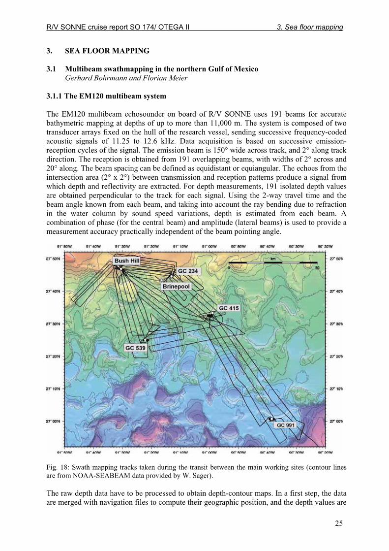
The EM120 multibeam echosounder on board of R/V SONNE uses 191 beams for accurate bathymetric mapping at depths of up to more than 11,000 m. The system is composed of two transducer arrays fixed on the hull of the research vessel, sending successive frequency-coded acoustic signals of 11.25 to 12.6 kHz. Data acquisition is based on successive emission-reception cycles of the signal. The emission beam is 150° wide across track, and 2° along track direction. The reception is obtained from 191 overlapping beams, with widths of 2° across and 20° along. The beam spacing can be defined as equidistant or equiangular. The echoes from the intersection area (2° x 2°) between transmission and reception patterns produce a signal from which depth and reflectivity are extracted. For depth measurements, 191 isolated depth values are obtained perpendicular to the track for each signal. Using the 2-way travel time and the beam angle known from each beam, and taking into account the ray bending due to refraction in the water column by sound speed variations, depth is estimated from each beam. A combination of phase (for the central beam) and amplitude (lateral beams) is used to provide a measurement accuracy practically independent of the beam pointing angle.
Fig. 18: Swath mapping tracks taken during the transit between the main working sites (contour lines are from NOAA-SEABEAM data provided by W. Sager). The raw depth data have to be processed to obtain depth-contour maps. In a first step, the data are merged with navigation files to compute their geographic position, and the depth values are

R/V SONNE cruise report SO 174/ OTEGA II 3. Sea floor mapping
26
plotted on a regular grid to obtain a digital terrain model (DTM). The grid has to be interpolated and finally smoothed to obtain a better graphic representation. Together with depth measurements, the acoustic signal is sampled each 3.2 ms and processed to obtain a cartographic mosaic, where gray levels are representative of backscatter amplitudes. The data provide information on the seafloor nature and texture. 3.1.2 Seafloor mapping at the northern Gulf of Mexico
During the SO 174 cruise, the SIMRAD EM120 swath bathymetry system which has been installed on R/V SONNE since June 2001, was used continuously, parallel with dedicated PARASOUND surveys and OFOS deployments. Bathymetric data were processed routinely onboard during the survey, using the NEPTUNE software from SIMRAD, which is available on board and the academic software MB-system from Lamont-Doherty Earth Observatory. Especially night transits between daily sampling stations and lander deployments were used for bathymetric surveys. In Figure 18 examples of survey tracks between Bush Hill, GC234, GC415 and GC539 are shown. These surveys at water depths between 500 and 1000 m yielded high-quality data covering an area of 350 km2 which notably improved the resolution of the bathymetry coverage (compare the resolution between Figs. 18 and 19). Two transits to GC991 meant an enormous southeast enlargement of the mapped area. The area shows a rough topography (Figure 19) at the northern Gulf of Mexcio slope reflecting the deformation caused by salt tectonics underneath.
Fig. 19: Swath bathymetry map of the Green Canyon measured by the SIMRAD EM120 system on board R/V SONNE during SO 174/4.

R/V SONNE cruise report SO 174/ OTEGA II 3. Sea floor mapping
27
In general the mapped area shows the hummocky topography which is typical for most parts of the Texas-Louisiana Slope formed by salt ascent beneath the seafloor (Bryant et al. 1991). In more detail, the area shows the transition from isolated salt diapirs, which are common on the shelf and upper slope, to the middle and lower slope which is more characterized by extensive salt sheets stretching south to the Sigsbee Escarpment (Sager et al. 2003). Therefore the topography in the northeast of this area (Figure 19) has a slope character dominated by small subcircular to elongated basins and salt massifs, the former occurring where the salt is thin or absent (Bryant at al. 1991). The mobile salt has extensively fractured the overlying sediments with regional growth faults.
3.2 Sub-bottom profiling and plume imaging
Andrea Gerriets, Florian Meier and Donald Shea Maddox
3.2.1 System Description PARASOUND
The PARASOUND sediment echosounder designed by ATLAS Hydrographic is a system installed permanently on R/V SONNE. It determines the water depth and detects variable frequencies from 2.5 up to 5.5 kHz thereby providing high-resolution information of the sedimentary layers at depths of up to 200 m below sea floor. For the sub-bottom profiler task, the system uses the parametric effect, which produces additional frequencies through non-linear acoustic interaction of finite amplitude waves. If two sound waves of similar frequencies (18 kHz, 22 kHz) are emitted simultaneously, a signal of the resulting frequency (e.g. 4 kHz) is generated for sufficiently high primary amplitudes. The new component is travelling within the emission cone of the original high frequency waves, which are limited to an angle of 4° for the equipment used. The resulting footprint size of 7% of the depth is much smaller than for conventional systems and both vertical and lateral resolutions are significantly improved. The PARASOUND system sends out a burst of pulses at 400-ms intervals until the first echo returns. The coverage of this discontinuous mode depends on the water depth, and produces non-equidistant shot intervals between bursts.
Fig. 20: PARASOUND DS-2 simulation: DAU interface

R/V SONNE cruise report SO 174/ OTEGA II 3. Sea floor mapping
28
ParaDigMA
For about 10 years the ATLAS PARASOUND system has been equipped with the associated DOS based data acquisition system ParaDigMA developed by V. Spieß (1993, University of Bremen). The ParaDigMA software offers visualization as well as digitization and storage of acoustic soundings. Today the combination of the PARASOUND echosounder DS-2 designed by ATLAS Hydrographic and ParaDigMA has accomplished the step from DOS towards a Windows platform and network capability. In a cooperation between ATLAS Hydrographic and the Department of Earth Sciences, University of Bremen, a new release of the PARASOUND/ParaDigMA system has been developed in order to adapt the system to modern requirements and provide improved features to survey the physical state of the sea floor along the ship's track as well as a high level of data quality. The new Windows ParaDigMA is commercially available as PARASTORE 3. It is designed for the ATLAS PARASOUND DS-2 system and does not work automatically with the system on R/V SONNE. In order to make the new Windows ParaDigMA available for the old PARASOUND control system, a supplemental interface application has been developed and in a second step adapted to the vessel's special environment. The DAU-Interface program (DAU = Short name of the old HP 3852 Data Acquisition Unit) simulates the new PARASOUND control system. On the one hand it communicates with and acquires the data from the old PARASOUND system like the former DOS software did. On the other hand it provides the data to the Windows ParaDigMA software like the new PARASOUND DS2 control system would. Concrete advantages of the Windows platform for PARASOUND watchkeepers and responsibles are the multithreaded programming structure and the network capability. E.g., paper jams in the printer do not longer stop the whole registration. The registered data are immediately available now and can be transferred via the network to processing computers at any location without stopping the registration. The registration window can be expanded by to 400 m without reducing the sampling rate. The expansion of the registration window combined with the new logarithmic color scale option proved to be an essential requirement for a successful bubble plume detection, since most of the detected methane plumes have a length of several hundreds of meters. Finally the improved interactive graphical user interface makes the application more user-friendly than before. In addition, a first step into the direction of "Remote PARASOUND" has been taken by the installation of a remote station in the OFOS laboratory. Such remote stations cannot control the echosounder but enable an online visualization of the current soundings at each location with LAN access on the vessel. During the SO 174/1 cruise both ParaDigMA versions, the DOS and the Windows version, were operated. DOS ParaDigMA was used for the registration of the standard 4kHz parametric signal that provides information about the sedimentary structure of the sub-bottom. Windows ParaDigMA was used for the registration of the 18-kHz NBS signal. The NBS registration was expected to provide information about locations and sizes of methane bubble plumes. So the object of interest during NBS registration was not the sub-bottom but the water column.

R/V SONNE cruise report SO 174/ OTEGA II 3. Sea floor mapping
29
For the 18-kHz NBS registration a separate acquisition system with a separate HP 3852A Data Acquisition Unit was installed. Therefore all serial navigation data and PARASOUND control data were splitted by a special serial interface splitter box designed and installed by the WTD.
Fig. 21: PARASOUND / ParaDigMA system architecture on SO 174/1.

R/V SONNE cruise report SO 174/ OTEGA II 3. Sea floor mapping
30
Fig. 22: New PARASOUND front end: WINDOWS ParaDigMa.
3.2.2 System operation
4-kHz parametric profiles
4-kHz parametric profiles provide information about the seafloor morphology and the structure of sedimentary layers along the ship's track. During parametric profiles, the PARASOUND system was operated in deep sea at water depths of more than 3000 m as well as in shallower water at water depths of about 400 m. The profiles were run with a speed of ~12 knots. The source signal was a band-limited, 2-6-kHz sinusoidal wavelet of a 4-kHz dominant frequency with a duration of 1 period. The seismograms were sampled at a frequency of 40 kHz, with a typical registration length of 266 ms for a depth window of 200 m. For the online visualization the echogram sections were filtered with a wide band pass filter to improve the signal-to-noise ratio. In addition, the data were normalized to a constant value much smaller than the average maximum amplitude thus amplifying deeper and weaker reflections. This online pre-processing only concerns data visualized on screen and plotted. The raw data stored in PS3 files do not pass any of the filters mentioned above. Since ParaDigMA provides a colored online plot the b/w analogue printout of the DESO 25 device was not operated during this cruise. The following problem concerning the communication of the serial PARASOUND control data occured for several days: The DOS ParaDigMA program did not recognize incoming control data from the PARASOUND system. Echosounder status values - for instance registration window, range or registration modes - were not updated. As a result the header values of the corresponding registered data will have to be corrected for further processing. Stopping and restarting the DOS ParaDigMA proved to be only a temporary solution.
18kHz Flare imaging profiles (NBS)
During 18-kHz NBS profiles, the PARASOUND system was operated at depths of up to 1500 m as well as in shallower areas with water depths of about 400 m. The source signal was a sinusoidal wavelet of a 18-kHz frequency with a duration of 4 periods. The 'CHANNEL SELECT' option was set to 'PAR' irrespective of the water depth. The beam width was set to an angle of 20°. The seismograms have been sampled at 40 kHz, with an increased registration length of 532 ms for a depth window of 400 m. The color scale was set to logarithmic scale.

R/V SONNE cruise report SO 174/ OTEGA II 3. Sea floor mapping
31
The NBS profiles were registered at ship's speeds of ~3 and ~5 knots, or ~0.5 knots during OFOS tracks. In combination with a low ship's speed the above mentioned echosounder settings allowed us a very clear visualization of bubble plumes that were passed during the survey. We were thus able to get relatively reliable information about the existence of bubble plumes within a limited area. The ranges of 2000 m and 500 m were operated without any serious problems. The 1000-m range proved to be problematic for flare imaging tasks. The data quality was affected by an extremely high noise in this range which made it almost impossible to visualize weak reflexions as produced by bubbles in the water column. Even if the ship passed directly over a plume, the flare disappeared due to the noise in the 1000-m range, so that we finally avoided to use the 1000-m range for flare imaging profiles. The flare imaging profiles were supposed to provide information about the existence, location and the rough quality of bubble plumes in areas where either plumes had already been found or slicks indicated the existence of submarine gas releases. The data acquired by the flare imaging profiles provided information to find appropriate locations for gas quant lander stations. All PARASOUND data are stored in digital PS3 format on CD-ROM and DAT-DDS2 data cartridges. Attached to these digital data, you find the original online plots of the parametric results and tables with the navigation data. All data have been archived by the University of Bremen, MTU AG Prof.Dr.V.Spieß. The post-processing of the PARASOUND data, as presented in the figures of this article, has been carried out with the application and SeNT (H.v.Lom, University of Bremen, 1995). 3.2.3 Preliminary results
Parametric profiles
The Gulf of Mexico (GOM) formed during the Jurassic as rifting occured between North and South America, forming an intercontinental sea. Due to high rates of evaporation, a thick layer of salt was deposited on the northern syn-rift sediments (Pindell et al. 1985). The salt layer was later buried by late Mesozoic and Cenozoic sediments, creating a thick continental margin sedimentary wedge (McGookey et al. 1975). The underlying salt is mobile under pressure, and diapirs and salt sheets have formed by its migration. These diapirs and salt sheets have displaced the sediment column in the northern GOM, forming salt domes and withdrawal basins. The PARASOUND data collected on cruise SO 174 image the effects of these domes and basins as tilted strata reflectors on top of salt bodies and horizontal strata reflectors above withdrawal basins (Figure 23). In the GOM, hydrates form on ridges of salt domes caused by faulting associated with salt migration. These faults intersect deep hydrocarbon reservoirs, so that migrating hydrocarbons can reach the seafloor (Sasson et al. 2001). Where faults outcrop on the seafloor, they are often accompanied by a formation of mud volcanoes and hydrate mounds. Features associated with these structures were imaged by the PARASOUND sub-bottom profiler. Figure 23 displays a section of data through GC185 and shows a mound, fault system, and acoustic wipeout below the mound associated with gassy sediments. Fault scarps outcrop on the seafloor on either side of the hydrate mound, serving as a pathway for hydrocarbons to the seafloor. Acoustic wipeout is imaged directly beneath the mound due to the scattering of acoustic energy by gassy sediments. Sediment failure and resulting slumps are common in the GOM due to the high slope angles of salt domes and active salt tectonics. The PARASOUND sub-bottom profiler

R/V SONNE cruise report SO 174/ OTEGA II 3. Sea floor mapping
32
imaged numerous layers interpreted as slumps. These data revealed large lenses of unconsolidated sediment ~ 10 m in thickness along the flanks of salt diapirs (Figure 24).
Fig. 23: PARASOUND image of sediments overlying a salt dome.
Fig. 24: Transparent lenticular insertions between the sediment layers.

R/V SONNE cruise report SO 174/ OTEGA II 3. Sea floor mapping
33
Flare imaging profiles (NBS)
Flare imaging profiles were run at the sites GC234, GC415, GC539 and GC991. The registration was further active during OFOS tracks.
Flare B Flare A Flare C
Flare A Flare B
Flare C
Flare A
S
W E
N
Profile 1
Profile 14 (inv.)
Profile 3
Profile 5
Fig. 26: Flare Imaging Site GC234. 3 flares detected on parallel profile lines at about 500 m water depth.
Fig. 25: Flare Imaging Site GC415. Flares detected at about 950 m water depth.

R/V SONNE cruise report SO 174/ OTEGA II 3. Sea floor mapping
34
Figure 25 shows 3 clear bubble plumes of more than 200 m in length at site GC234. The flares were detected at a speed of 3 kn and with a range of 500. Concerning the quality of the visual results this site was the most successful of SO 174/1. The distance between the profile lines was chosen small enough to detect one single plume on 3 different of the parallel profiles. As a result, on GC234 in 10 of 15 profiles the data showed gas plumes in the water column. Figure 26 shows flares that were detected at 5 kn with a range of 2000 at a water depth of more than 900 m at site GC415. The rather lower horizontal resolution combined with some interferences was probably caused by the higher range. 3.3 Multibeam echosounding and PARASOUND on the Sigsbee and Campeche Knolls
Paul Blanchon, Carlos Mortera and Florian Meier Bathymetric swath data were collected with a SIMRAD EM120 Multibeam Echo Sounder (MBES) utilising a 12 kHz sonar frequency with 191 beams and an angular coverage of 120�. This setup provided swaths of up to 4 times the depth and a spatial resolution of 15 m. Certain substrate conditions, such as abyssal soupy substrates, caused significant bathymetric artifacts that needed to be removed during data processing. All maps shown here, however, are preliminary and based on pre-processed data. Subsurface sediment profiles were collected with an Atlas PARASOUND narrow-beam echo-sounder and subottom profiler with a footprint diameter of 7% of the water depth. The system utilizes the parametric effect, which arises from non-linear interaction between high frequency sound waves of finite amplitude (18-25 kHz). An interference frequency between 2.5 and 5.5 kHz is generated, which is focusses to a cone with an operating angle of 4 degrees. The vertical resolution of the PARASOUND system is in the order of a few decimeteres and, for the surveys reported here, signal penetration varied between 5 to 80 m. Several substrate conditions caused deterioration in signal penetration. It was found, for example, that profiles run perpendicular to slope contours (even if the slopes were < 2�) had particularly poor signal penetration (<30m) compared to profiles run parallel to depth contours. In addition, PARASOUND uses a general sound-velocity in water of 1500 m/s and therefore does not accurately calculate depth below the sediment/water interface.
Continuous (MBES) swaths and PARASOUND subottom profiles were collected from two rectangular areas in the southern Gulf of Mexico: a 30 by 55 km area encompassing 5 of the Sigsbee Knolls and 60 by 110 km area encompassing 22 of the northern Campeche Knolls (Figs. 4 and 16). The objective was to produce a high-resolution bathymetric map and investigate the shallow subsurface structure in order to identify processes which have controlled the surface form and development of these structures and the sedimentary deposits surrounding them. Limited profiles and swath data were also collected from the Campeche margin to look for relic shorelines. Although several shorelines were identified, the limited extent of the data prevents a useful discussion here. This report therefore concentrates on the deep-water knolls where extensive data are available. Discovered by Ewing in 1954, the Sigsbee Knolls are large salt diapirs which pierce and deform the extensive abyssal plain in the center of the Gulf of México. Cores taken from one of the knolls, known as 'Challenger knoll', during DSDP leg 2 contained oil and penetrated 144 m of insoluble-residue cap-rock containing anhydrite, gypsum, calcite and native sulphur. The cap consisted of an upper calcite zone, underlain by a transitional zone with gypsum and sulphur and a thick lower layer of Anhydrite before passing into rock-salt. Age of the salt was biostratigraphically determined to be mid-late Jurassic (Kirkland and Gerhard 1971). Early

R/V SONNE cruise report SO 174/ OTEGA II 3. Sea floor mapping
35
work on cap rocks had shown that hydrocarbon seeps associated with diapirs allowed bacteria-mediated reactions to convert anhydrite to biogenic calcite and hydrogen sulphide (Feely and Kulp 1957). The hydrogen sulphide is subsequently converted to elemental sulphur (which forms commercial deposits in some cap rocks). Salt which forms the Sigsbee Knolls is an extension of a deposit that underlies the entire slope region and extends into the Bay of Campeche where it forms an almost continuous salt mass. This mass feeds many large diapirs and ridges which fault and fold the overlying sediment package and rise to within 1000 m of the surface but generally do not break the sea floor. The domes are associated with major oil accumulations which form the marine Campeche Oil fields. To the north of these large oil-bearing features, are the Northern Campeche Knolls, where the salt is thinner producing more isolated salt diapirs which penetrate the sea-floor forming knolls with up to 1500 m of relief (Bryant et al. 1991). Between the salt diapirs of the abyssal deep-sea regions, sediments consist largely of muddy laminites deposited during the Pleistocene and Holocene. DSDP leg 10 recovered cores from the Sigsbee Abyssal Plain and found these sediments to be in excess of 510 m thick consisting of homogenous gray nanofossil clay sometimes mottled or faintly laminated, as well as graded fine sands and silts associated with distal turbidites (Davies 1968; Worzel et al 1973). Sigsbee Knolls MBES swath mapping shows the Sigsbee Knolls to be roughly equidimensional domes ranging in diameter from 6 to 11 km but averaging ~8 km (Figure 27). They range in relief above the surrounding sediment floor from ~150 to 300 m and have maximum slopes of between 20 and 25%. PARASOUND profiles crossed 4 of the salt diapirs and each displayed a typically attenuated acoustic signal. Sediment lenses >20 m thick are detectable over the crest and flanks of each diapir, filling the highly irregular and possibly faulted topography of the salt surface and producing relatively smooth domes. As a consequence, they show relatively little surface sculpturing apart from isolated peaks on the crest of the knolls (Figure 28).
Fig. 27: Swath bathymetry map of the Sigsbee Knolls survey area; each knoll is numbered according to the latitude of its highest point. Note also the swath artifacts which may reflect heavy swell conditions during the survey.

R/V SONNE cruise report SO 174/ OTEGA II 3. Sea floor mapping
36
Fig. 28: Example of a PARASOUND profile across a piercement salt diapir (2315) surveyed on the Sigsbee Plain. The profile shows sediment onlap and in-filling of the irregular relief of the salt surface as well as the attenuated acoustic signal that is so typical of salt bodies. Sediment layers in the upper 60 m of Sigsbee basin are clearly resolved by PARASOUND profiles across the entire width of the survey area (30 x 55 km) and up to the continental rise of the Campeche Bank over 100 km away. These deposits consists of 4, laterally continuous, ~15 m-thick sequences. Each sequence starts with a 6-m-thick basal transparent unit which is overlain by 7 m of meter-thick alternating beds and finally capped by 2 m of alternating submeter-thick beds. These 4 sequences and their individual layers are laterally continuous for 100's of kilometers with almost no change in thickness (Figure 29). The only changes in thickness occur where they onlap steeper slopes associated salt diapirs and the continental rise, and in the Campeche Knolls area where the sequences become less distinct. In terms of internal consistency between sequences, the number and thickness of layers varies slightly between sequences. The deeper sequences are thinner and contain fewer of the thinner layers than sequences above. This minor variability is likely the result of greater dewatering and compaction in the deeper sequences especially given that the thickness and number of layers increase in successively shallower sequences.

R/V SONNE cruise report SO 174/ OTEGA II 3. Sea floor mapping
37
Fig. 29: PARASOUND profiles from widely spaced locations showing almost identical and laterally-continuous sequences. Four sequences can be recognized (S1-S4) and each sequence starts with a megaturbidite (MT). Note also there is a slight thickening towards the center of the basin at Sigsbee. All depths shown in meters below mean sea level. Northern Campeche Knolls
Fig. 30: Swath bathymetry map of thenorthern Campeche Knolls survey areawith knolls numbered according tolatitude. Also shown are colored dotsshowing surface seep-indications fromsatellite data (light dots) and asphaltclasts or flows identified on video-sledtransects.

R/V SONNE cruise report SO 174/ OTEGA II 3. Sea floor mapping
38
Multibeam swath data show the northern Campeche Knolls to be elongated 'pillows' up to 24 km in length and 10 km in width but averaging roughly 5 by 10 km. Of the 22 knolls mapped, 4 are oriented roughly north south and the rest have a north-west south-east alignment. They range in relief above the surrounding sediment floor from ~450 to 800 m and have maximum slopes of between 20 and 30% (Figure 30). Approximately half of the knolls mapped have crests and flanks dissected by either crescentic or linear scarps which may correspond to slump scars and faults respectively. In many cases the crescentic scarps are associated with down-slope sediment lobes which extend significant distances (up to 4 km) out over the adjacent sea floor (Figure 31). These 'dissected' knolls are also associated with surface oil-seep slicks identified from satellite data and, at least in one case, tar flows have been discovered (during this expedition) covering the upper flanks of a knoll. PARASOUND profiles crossed 18 of the 22 knolls and confirmed that they are piercement-type salt diapirs with steep flanks and an irregular crestal surface (indicated by the attenuated acoustic signal). Where crestal sediment layers could be identified, they were found to be thinner (<20 m) than those associated with the Sigsbee Knolls.
Fig. 31: High resolutionswath map of a dissectedknoll (2137) showing a largecrescentic scarp and a down-slope sediment lobe thatextends a significant distanceout onto the abyssal plain.These features areinterpreted to be the result ofmass-wasting induced byeither the interactionbetween tar flows and gas-hydrate-bearing sediment orthe loading of tar on water-saturated sediments built upon the flanks of the knoll.
In contrast to the high penetration at Sigsbee, sediment layers in the Campeche Knolls area can only be resolved down to ~40 m below the sea floor. As a consequence only the upper 3 of the previously identified 15 m-thick sequences can be recognized. The best areas to see these sequences in their entirety is the flat sea floor between salt diapirs because sequence distinction is lost as the sediment layers rise and drape the steeper slopes of adjacent diapirs (signal penetration also deteriorates as slope increases). If these areas are avoided however, it is possible to recognize distinct changes in thickness across the area. In the north, sequences are

R/V SONNE cruise report SO 174/ OTEGA II 3. Sea floor mapping
39
comparable to those at Sigsbee having the same overall thickness and similar bed thicknesses. But sections to the south differ significantly. Here the basal transparent unit of sequence 2 is thicker (8-9 m compared to 6 m at Sigsbee) and the muddy upper two-thirds of sequence 1 is missing. These changes may indicate that the source of sand and silt that produces the basal transparent layer lies somewhere to the south of the area (perhaps the Bay of Campeche) whereas the source of the alternating beds lies further north (perhaps the Mississippi Delta).
Sediment sequences
Cores from the Sigsbee abyssal plain recovered by DSDP leg 10 showed that much of the Holocene and Pleistocene section is composed of meter-thick units of very fine sand grading to silt which thin into the basin (Worzel et al 1973). Based on this evidence, Beall et al (1973) suggested that each fining-up unit represented the distal parts of individual turbidite flows. This turbidite interpretation corresponds well with the layered sequences we have identified from the PARASOUND profiling. The thicker transparent units seen at the base of each sequence probably represent several superimposed sand-and-silt dominated turbidites which produce a thick seismic unit by virtue of the minimal velocity contrast between layers, whereas the smaller-scale alternations of reflectors higher in the sequence likely represent individual turbidites separated by thicker 'background' clays thereby producing larger velocity contrasts. The layering pattern within each sequence therefore seems to represent a basal stage dominated by an almost continuous influx of turbidites followed by subsequent stages where turbidites gradually become less frequent. Given that turbidite grain size and thickness generally decrease away from the source (e.g. Rupke 1975; Ricci-Lucci and Valmori 1980), the decrease in turbidite frequency seen in each sequence probably represents a gradually increasing distance from the source forced by eustatic sea-level rise (Shanmugam and Moiola 1984). As such, more frequent turbidites at the base of each sequence would represent lowstand conditions during glaciation when fluvial point sources moved down-shelf towards the basin (Rothwell et al. 2000). Similarly, the increasing proportion of muds toward the top of the sequence would signify rising sea level during deglaciation and, ultimately, highstand conditions when fluvial sources retreated up-shelf to their farthest distance from the basin. However, this simple sea-level control on sediment layering does not entirely fit the sequence observed because there appears to be no record of gradually increasing turbidite thickness as sea-level falls from the highstand. Instead, each sequence starts with an abrupt change in thickness, which essentially indicates an abrupt transition from highstand deposition to lowstand deposition implying that sea-level fall from the highstand was rapid and very little record was preserved. This record therefore produces a sawtooth pattern of change (that is so characteristic of other glacial-interglacial records) rather than a sinusoidal pattern. If the pattern of layering in these sequences is indeed controlled by sea-level changes during glacial-interglacial cycles, and each sequence represents a lowstand to highstand succession that lasted ~100,000 years, then it is possible to calculate the average sedimentation rate for each sequence. Ignoring the effects of sediment compaction, the maximum thickness for the youngest sequence is 17 m giving a sedimentation rate of 0.17 mm/yr. This compares well with similar units found in abyssal plains of the Mediterranean Sea where a maximum thickness of 20 m is reported for the youngest glacial lowstand to Holocene highstand turbidite sequence (Rothwell et al 2000).
Significance of dissected knolls
Faulting around salt diapirs is well documented and usually takes two forms, radial faults and

R/V SONNE cruise report SO 174/ OTEGA II 3. Sea floor mapping
40
keystone grabens. Both types form in response to relative uplift of the diapir which causes stress in both flanking sediments and those draping the crest of the structure (Nelson 1991). These fault types are only recognized from swath maps over the northern Campeche Knolls where most of the faulting occurs on the larger salt pillows. Keystone grabens are present on two large pillows (see 2154 and 2124 on Figure 30) and flank faulting occurs on at least 7 of the diapirs. The absence of faulting on the Sigsbee Knolls may be attributed to their generally smaller relief and therefore lesser amounts of uplift. In contrast to faulting, the crescentic scarps and the downslope sediment lobes are more enigmatic and have not been reported from other submerged salt structures. Although these structures are clear evidence of mass wasting, the cause of the instability is uncertain. Three main possibilities exist: 1. seismicity-associated salt tectonics, 2. slope failure induced by diapir uplift or, 3. interaction between tar flows and gas hydrate in initiating sediment instability. Given that at least half of the salt diapirs in the northern Campeche Knoll field show evidence of faulting, the first two potential causes, which relate directly to salt tectonics, are leading candidates. However the lack of previous reports of this type of mass wasting on other salt structures is puzzling given that faulting is such a common phenomenon on these structures (Nelson 1991). Although tar flows were only found on one knoll (2155), all salt structures with large slump scarps and sediment lobes seem to be associated with evidence of oil seeps, as shown from satellite data. If this association can be taken to indicate that tar flows also exist on other knolls, then there would be a much stronger case for the association between tar flows and sediment instability.
3.4 Visual seafloor observation
Anton Eisenhauer, Ian MacDonald, Friedrich Abegg and Olaf Pfannkuche The main aim of the visual seafloor observation program was locating active vent sites in the Gulf of Mexico (Campeche Escarpment, Sigsbee Knolls) and on the continental margins of the United States (GC415, Bush Hill Complex). We used the Ocean Floor Observation System (OFOS), which is a TV-guided sled of 165x125x145 cm equipped with a BW video camera, two Xenon lamps (Fa. OKTOPUS), an underwater slide camera with flash (Fa. Benthos), three laser pointers (Fa. OKTOPUS) and an FSI memory CTD. OFOS allows a precise detection of possible sampling sites for the TV-MUC and the TV-Grab. Furthermore, OFOS is also useful for the interpretation of sediment echosounder data or sidescan sonar mapping. For the seafloor observation procedure, OFOS is towed along a pre-defined track by the ship with less than 1 kn. The distance between the sled and the seafloor can be controlled manually by the winch. Pictures of the seafloor can be taken either continuously at set intervals or manually. In addition, the video signal of the camera is permanently recorded on video tape. During cruise SO 174/2 digital processing of the video signal and its DVD storage were tested. In addition to the ship-based recording of OFOS data during SO 174/2, the OFOS data were also stored using a protocol software which automatically recorded UTC time, ship position and other data from a NMEA-link/DVS online string.

R/V SONNE cruise report SO 174/ OTEGA II 3. Sea floor mapping
41
Digital imaging
Two experimental camera systems were deployed for during cruise SO 174/2 the first time. Both systems were successful in providing useful, high-resolution images, which were immediately available for analysis. These camera systems had been developed by Ian MacDonald through his relationship with the commercial firm AquaPix LLC.
The camera system used with OFOS, called SeaSnap 990, uses a Nikon Coolpix 990 camera modified for installation in a titanium housing with an optical dome. Illumination was provided by a Sea & Sea strobe (YS300) likewise mounted in a pressure housing. Control of the camera and strobe was accomplished by a preset digital timer, which was adjusted to fire the camera and strobe at regular intervals (e.g. 15 s) after an initial delay to allow the camera to be deployed to the bottom. The SeaSnap99O and its strobe were mounted on OFOS near the attachment point for the bottom weight (Fig 1). In this position, the digital camera produced an image of 1.5 x 1.1 m of the seafloor when OFOS was deployed at 3 m above the bottom. This high-resolution view was a good complement to the wide-angle views that were taken with the film camera. The SeaSnap 990 was deployed on eight OFOS dives and collected a total of 3337 digital bottom images. One of the dives (OFOS 10) was unsuccessful because the optical port of the housing became fogged with condensation.
Fig. 32: Ocean Floor Observation System (OFOS) inverted to show camera placements.
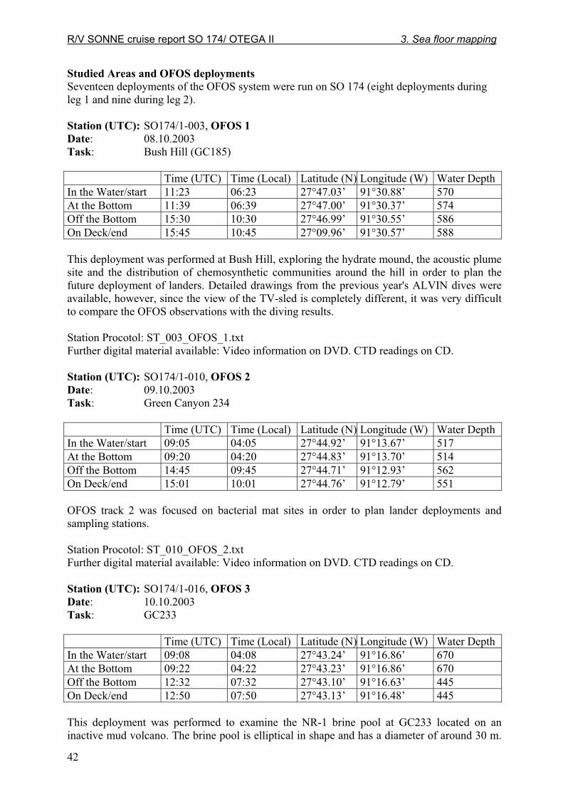
R/V SONNE cruise report SO 174/ OTEGA II 3. Sea floor mapping
42
Studied Areas and OFOS deployments
Seventeen deployments of the OFOS system were run on SO 174 (eight deployments during leg 1 and nine during leg 2). Station (UTC): SO174/1-003, OFOS 1 Date: 08.10.2003 Task: Bush Hill (GC185) Time (UTC) Time (Local) Latitude (N) Longitude (W) Water Depth In the Water/start 11:23 06:23 27°47.03’ 91°30.88’ 570 At the Bottom 11:39 06:39 27°47.00’ 91°30.37’ 574 Off the Bottom 15:30 10:30 27°46.99’ 91°30.55’ 586 On Deck/end 15:45 10:45 27°09.96’ 91°30.57’ 588 This deployment was performed at Bush Hill, exploring the hydrate mound, the acoustic plume site and the distribution of chemosynthetic communities around the hill in order to plan the future deployment of landers. Detailed drawings from the previous year's ALVIN dives were available, however, since the view of the TV-sled is completely different, it was very difficult to compare the OFOS observations with the diving results. Station Procotol: ST_003_OFOS_1.txt Further digital material available: Video information on DVD. CTD readings on CD.
Station (UTC): SO174/1-010, OFOS 2 Date: 09.10.2003 Task: Green Canyon 234 Time (UTC) Time (Local) Latitude (N) Longitude (W) Water Depth In the Water/start 09:05 04:05 27°44.92’ 91°13.67’ 517 At the Bottom 09:20 04:20 27°44.83’ 91°13.70’ 514 Off the Bottom 14:45 09:45 27°44.71’ 91°12.93’ 562 On Deck/end 15:01 10:01 27°44.76’ 91°12.79’ 551 OFOS track 2 was focused on bacterial mat sites in order to plan lander deployments and sampling stations. Station Procotol: ST_010_OFOS_2.txt Further digital material available: Video information on DVD. CTD readings on CD. Station (UTC): SO174/1-016, OFOS 3
Date: 10.10.2003 Task: GC233 Time (UTC) Time (Local) Latitude (N) Longitude (W) Water Depth In the Water/start 09:08 04:08 27°43.24’ 91°16.86’ 670 At the Bottom 09:22 04:22 27°43.23’ 91°16.86’ 670 Off the Bottom 12:32 07:32 27°43.10’ 91°16.63’ 445 On Deck/end 12:50 07:50 27°43.13’ 91°16.48’ 445 This deployment was performed to examine the NR-1 brine pool at GC233 located on an inactive mud volcano. The brine pool is elliptical in shape and has a diameter of around 30 m.
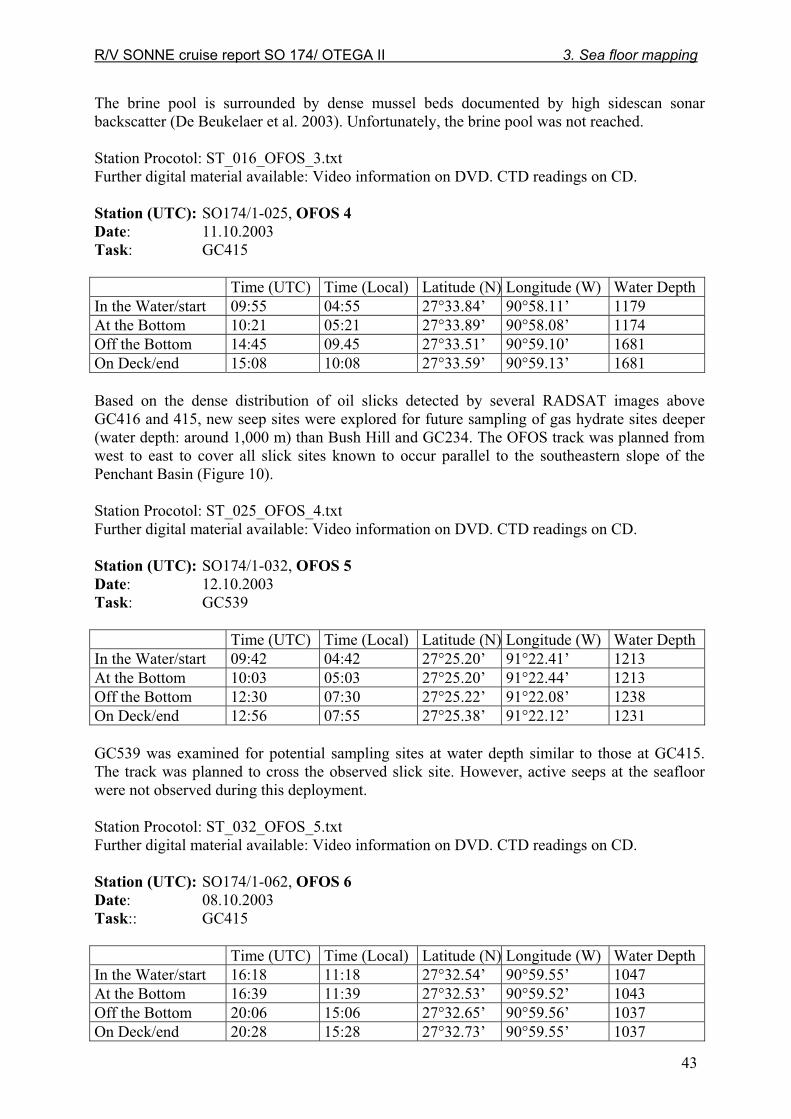
R/V SONNE cruise report SO 174/ OTEGA II 3. Sea floor mapping
43
The brine pool is surrounded by dense mussel beds documented by high sidescan sonar backscatter (De Beukelaer et al. 2003). Unfortunately, the brine pool was not reached. Station Procotol: ST_016_OFOS_3.txt Further digital material available: Video information on DVD. CTD readings on CD. Station (UTC): SO174/1-025, OFOS 4 Date: 11.10.2003 Task: GC415 Time (UTC) Time (Local) Latitude (N) Longitude (W) Water Depth In the Water/start 09:55 04:55 27°33.84’ 90°58.11’ 1179 At the Bottom 10:21 05:21 27°33.89’ 90°58.08’ 1174 Off the Bottom 14:45 09.45 27°33.51’ 90°59.10’ 1681 On Deck/end 15:08 10:08 27°33.59’ 90°59.13’ 1681 Based on the dense distribution of oil slicks detected by several RADSAT images above GC416 and 415, new seep sites were explored for future sampling of gas hydrate sites deeper (water depth: around 1,000 m) than Bush Hill and GC234. The OFOS track was planned from west to east to cover all slick sites known to occur parallel to the southeastern slope of the Penchant Basin (Figure 10). Station Procotol: ST_025_OFOS_4.txt Further digital material available: Video information on DVD. CTD readings on CD. Station (UTC): SO174/1-032, OFOS 5 Date: 12.10.2003 Task: GC539 Time (UTC) Time (Local) Latitude (N) Longitude (W) Water Depth In the Water/start 09:42 04:42 27°25.20’ 91°22.41’ 1213 At the Bottom 10:03 05:03 27°25.20’ 91°22.44’ 1213 Off the Bottom 12:30 07:30 27°25.22’ 91°22.08’ 1238 On Deck/end 12:56 07:55 27°25.38’ 91°22.12’ 1231 GC539 was examined for potential sampling sites at water depth similar to those at GC415. The track was planned to cross the observed slick site. However, active seeps at the seafloor were not observed during this deployment. Station Procotol: ST_032_OFOS_5.txt Further digital material available: Video information on DVD. CTD readings on CD. Station (UTC): SO174/1-062, OFOS 6 Date: 08.10.2003 Task:: GC415 Time (UTC) Time (Local) Latitude (N) Longitude (W) Water Depth In the Water/start 16:18 11:18 27°32.54’ 90°59.55’ 1047 At the Bottom 16:39 11:39 27°32.53’ 90°59.52’ 1043 Off the Bottom 20:06 15:06 27°32.65’ 90°59.56’ 1037 On Deck/end 20:28 15:28 27°32.73’ 90°59.55’ 1037
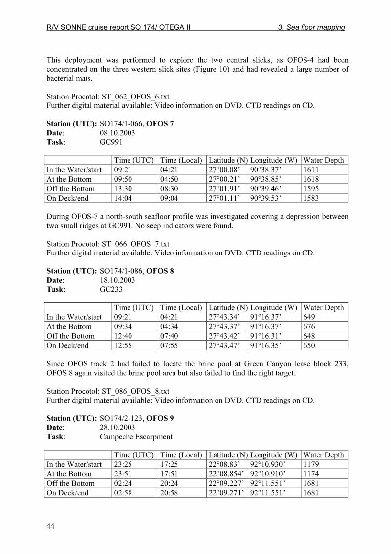
R/V SONNE cruise report SO 174/ OTEGA II 3. Sea floor mapping
44
This deployment was performed to explore the two central slicks, as OFOS-4 had been concentrated on the three western slick sites (Figure 10) and had revealed a large number of bacterial mats. Station Procotol: ST_062_OFOS_6.txt Further digital material available: Video information on DVD. CTD readings on CD. Station (UTC): SO174/1-066, OFOS 7
Date: 08.10.2003 Task: GC991 Time (UTC) Time (Local) Latitude (N) Longitude (W) Water Depth In the Water/start 09:21 04:21 27°00.08’ 90°38.37’ 1611 At the Bottom 09:50 04:50 27°00.21’ 90°38.85’ 1618 Off the Bottom 13:30 08:30 27°01.91’ 90°39.46’ 1595 On Deck/end 14:04 09:04 27°01.11’ 90°39.53’ 1583 During OFOS-7 a north-south seafloor profile was investigated covering a depression between two small ridges at GC991. No seep indicators were found. Station Procotol: ST_066_OFOS_7.txt Further digital material available: Video information on DVD. CTD readings on CD. Station (UTC): SO174/1-086, OFOS 8 Date: 18.10.2003 Task: GC233 Time (UTC) Time (Local) Latitude (N) Longitude (W) Water Depth In the Water/start 09:21 04:21 27°43.34’ 91°16.37’ 649 At the Bottom 09:34 04:34 27°43.37’ 91°16.37’ 676 Off the Bottom 12:40 07:40 27°43.42’ 91°16.31’ 648 On Deck/end 12:55 07:55 27°43.47’ 91°16.35’ 650 Since OFOS track 2 had failed to locate the brine pool at Green Canyon lease block 233, OFOS 8 again visited the brine pool area but also failed to find the right target. Station Procotol: ST_086_OFOS_8.txt Further digital material available: Video information on DVD. CTD readings on CD. Station (UTC): SO174/2-123, OFOS 9 Date: 28.10.2003 Task: Campeche Escarpment Time (UTC) Time (Local) Latitude (N) Longitude (W) Water Depth In the Water/start 23:25 17:25 22°08.83’ 92°10.930’ 1179 At the Bottom 23:51 17:51 22°08.854’ 92°10.910’ 1174 Off the Bottom 02:24 20:24 22°09.227’ 92°11.551’ 1681 On Deck/end 02:58 20:58 22°09.271’ 92°11.551’ 1681
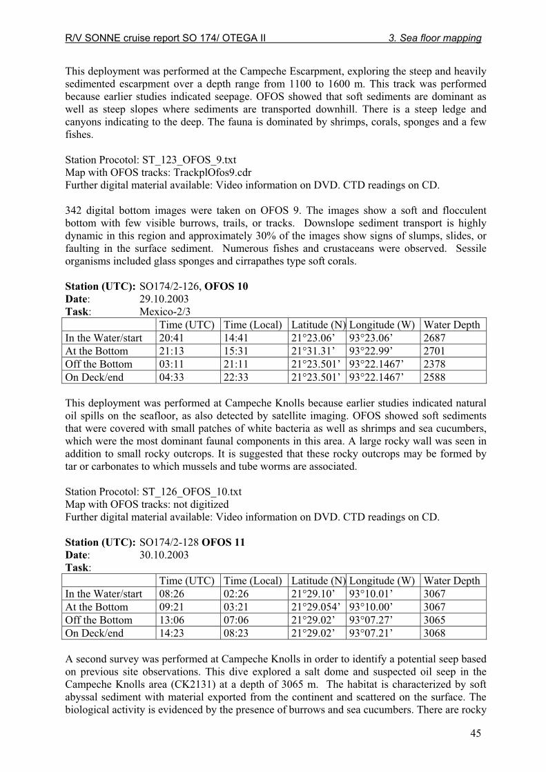
R/V SONNE cruise report SO 174/ OTEGA II 3. Sea floor mapping
45
This deployment was performed at the Campeche Escarpment, exploring the steep and heavily sedimented escarpment over a depth range from 1100 to 1600 m. This track was performed because earlier studies indicated seepage. OFOS showed that soft sediments are dominant as well as steep slopes where sediments are transported downhill. There is a steep ledge and canyons indicating to the deep. The fauna is dominated by shrimps, corals, sponges and a few fishes. Station Procotol: ST_123_OFOS_9.txt Map with OFOS tracks: TrackplOfos9.cdr Further digital material available: Video information on DVD. CTD readings on CD. 342 digital bottom images were taken on OFOS 9. The images show a soft and flocculent bottom with few visible burrows, trails, or tracks. Downslope sediment transport is highly dynamic in this region and approximately 30% of the images show signs of slumps, slides, or faulting in the surface sediment. Numerous fishes and crustaceans were observed. Sessile organisms included glass sponges and cirrapathes type soft corals. Station (UTC): SO174/2-126, OFOS 10 Date: 29.10.2003 Task: Mexico-2/3 Time (UTC) Time (Local) Latitude (N) Longitude (W) Water Depth In the Water/start 20:41 14:41 21°23.06’ 93°23.06’ 2687 At the Bottom 21:13 15:31 21°31.31’ 93°22.99’ 2701 Off the Bottom 03:11 21:11 21°23.501’ 93°22.1467’ 2378 On Deck/end 04:33 22:33 21°23.501’ 93°22.1467’ 2588 This deployment was performed at Campeche Knolls because earlier studies indicated natural oil spills on the seafloor, as also detected by satellite imaging. OFOS showed soft sediments that were covered with small patches of white bacteria as well as shrimps and sea cucumbers, which were the most dominant faunal components in this area. A large rocky wall was seen in addition to small rocky outcrops. It is suggested that these rocky outcrops may be formed by tar or carbonates to which mussels and tube worms are associated. Station Procotol: ST_126_OFOS_10.txt Map with OFOS tracks: not digitized Further digital material available: Video information on DVD. CTD readings on CD. Station (UTC): SO174/2-128 OFOS 11
Date: 30.10.2003 Task: Time (UTC) Time (Local) Latitude (N) Longitude (W) Water Depth In the Water/start 08:26 02:26 21°29.10’ 93°10.01’ 3067 At the Bottom 09:21 03:21 21°29.054’ 93°10.00’ 3067 Off the Bottom 13:06 07:06 21°29.02’ 93°07.27’ 3065 On Deck/end 14:23 08:23 21°29.02’ 93°07.21’ 3068 A second survey was performed at Campeche Knolls in order to identify a potential seep based on previous site observations. This dive explored a salt dome and suspected oil seep in the Campeche Knolls area (CK2131) at a depth of 3065 m. The habitat is characterized by soft abyssal sediment with material exported from the continent and scattered on the surface. The biological activity is evidenced by the presence of burrows and sea cucumbers. There are rocky

R/V SONNE cruise report SO 174/ OTEGA II 3. Sea floor mapping
46
outcrops and rocky walls, boulders to massifs. Typical fauna in this area are sea cucumbers, corals and sponges. Station Procotol: not digitized Map with OFOS tracks: not digitized Further digital material available: Video information on DVD. CTD readings on CD. 436 digital bottom images were taken on OFOS 11. The images show that the bottom sediments here were coarser grained than on the previous dive. Pteropod tests littered the bottom in many areas and evidence for active bioturbation was pervasive. Digital images showed various evidence of the chemosynthetic nature of this site. Numerous trails probably made by Calyptogena clams were photographed. Bacterial mats and living clams were seen in two images. Notably, one photograph shows what are clearly fragments of solidified bitumen (Figure 2). This demonstrates that the bitumen deposits found later at Chapopote were not restricted to that site.
Fig. 33: Bitumen deposits at CK22131. Weight is 20 cm long
Station (UTC): SO174/2-130 OFOS 12 Date: 31.10.2002 Task: Time (UTC) Time (Local) Latitude (N) Longitude (W) Water Depth In the Water/start 03:14 21:12:41 21°23.947’ 93°23,454’ 2402 At the Bottom 03:53 21:53:52 21°23.930’ 93°23,40’ 2425 Off the Bottom 07:17 01:30:00 21°23.710’ 93°23,22’ 2451 On Deck/end 08:17 02:16:00 21°23.840’ 93°22,13’ 2455 This was a downhill survey along a west-to-east transect. The track showed a normal seafloor with soft sediments characterized by a large number of burrows that provide the habitat with a rugged topography formed by ridges, depressions and tracks. The presence of isolated tube worms, bacterial mats and carbonates is documented along the track. The bacterial mats form small rounded patches. Along the track, flow structures were recognized in the sediments. These structures were later interpreted as tar flows or tar flow events. Bacteria are embedded in the flow suggesting different events that may cover existing fauna in the area. The tar flows support a local biological community composed of squat lobsters, shrimps, anemone and bivalves. Station Procotol: ST_123_OFOS_12.txt

R/V SONNE cruise report SO 174/ OTEGA II 3. Sea floor mapping
47
Map with OFOS tracks: TrackplOfos12.cdr Further digital material available: Video information on DVD. CTD readings on CD. Station (UTC): SO174/2-135 OFOS 13 Date: 01.11.2003 Task: Vent Survey Time (UTC) Time (Local) Latitude (N) Longitude (W) Water Depth In the Water/start 07:31 01:30 21°53.952’ 93°27.002’ 2972 At the Bottom n.d. n.d. 2972 Off the Bottom 14:43 08:43 21°53.885’ 93°26.217’ 2921 On Deck/end 15:26 09:26 21°54.008’ 93°26.184’ 2901 The track started on a large carbonate outcrop covered with tube worms and other fauna typical for this type of environment. The rocks ended abruptly, followed by abyssal soft sediment on which smaller rocks occurred as well as patches. These structures looked like tar flows, similar to lava flows. These outcrops include mussels, tube worms and bacterial mats. Some shrimps seem to be associated to the bacterial mats. The abyssal sediment slopes down and is characterized by animal tracks. Small boulders, similar to pillow lava, were scattered about the sediments. In the soft sediments, sea cucumbers occurred frequently. Station Procotol: ST_135_OFOS_13.txt Map with OFOS tracks: not digitized Further digital material available: Video information on DVD. CTD readings on CD. Station (UTC): SO174/2-138 OFOS 14 Date: 02.11.2003 Task: Chapopote Time (UTC) Time (Local) Latitude (N) Longitude (W) Water Depth In the Water/start 05:42 11:42 2882 At the Bottom 06:41 12:42 21°54.207’ 93°26.556’ 2882 Off the Bottom 11:01 17:01 21°54.222’ 93°25.351’ 2943 On Deck/end 11:54 17:54 21°54.222’ 93°25.351’ 2943 We started at the top of tar hill. The top of tar hill, named “Chapopote” (21°54.1250´N, 93°26.4730´W, 2882 m) consists of soft sediment without the presence of tar flows. Moving downslope, rocky structures were found with mussels, tube worms and shell fields. Squat lobsters are indicators of the presence of tar flows and occur associated to bacterial mats. This first tar structure is well delimited from the soft sediments. On the soft sediments, rocky outcrops rather appear downslope. Rocky structures occurred closer to the valley and looked like older flows that had been degraded by an “erosion”. They had lesser associated fauna and are heavily coated with soft sediments. There are only a few tube worms, occasionally surrounding small boulders. One of the rocky complexes is composed of twisted “rope-like” lava formations. Station Procotol: ST_138_OFOS_14.txt Map with OFOS tracks: TrackplOfos14.cdr Further digital material available: Video information on DVD. CTD readings on CD. 621 digital bottom images were taken on OFOS 14. The images include high-resolution photos of chemosynthetic fauna in close association with bitumen. The morphological variety of the bitumen deposits is clearly shown and provides strong evidence for liquid flow of this material.

R/V SONNE cruise report SO 174/ OTEGA II 3. Sea floor mapping
48
Also noteworthy was the relative scarcity of Beggiatoa mats. These bacteria are the most common component of the seeps on the northern Gulf of Mexico slope, but here they were restricted to a few localities. Where the Beggiatoa were found, authigenic carbonates could be seen on the surface, but they were absent elsewhere (Figure 34 left). The tar showed signs of bacterial colonization in the areas of the freshest flows. Here, a thick white film was photographed in the cracks and crevices of the tar flows (Figure 34 right). This may be Beggiatoa or it may be elemental sulfur excreted by sulfide-oxidizing vibrio.
Fig. 34: Bacterial mats at Chapopote. Left is a detail showing bacterial mats and carbonates at one of thefew locations where “typical” bacterial mats were present (DSCN5349.JPG). Right is a detail from freshbitumen flows in which possible bacterial mats or byproducts are lining the concave folds between layersof bitumen (DSCN5489mod.JPG) Station (UTC): SO174/2-145 OFOS 15
Date: 04.11.2003 Task: Sigsbee Knolls Time (UTC) Time (Local) Latitude (N) Longitude (W) Water Depth In the Water/start 09:35 03:35 23°28.669’ 92°27.179’ 3500 At the Bottom 10:36 04:35 23°28.666’ 92°27.101’ 3496 Off the Bottom 13:31 07:30 23°29.321’ 92°26.663’ 3717 On Deck/end 13:31 08:37 23°29.326’ 92°26.662’ 3717 This was a short survey at the Sigsbee Knoll 2328 that started along a downhill transect on only abyssal soft sediment. The benthic environment here includes more abundant mobile fauna. Life in this habitat is significantly more reduced than in the previous areas surveyed. The sediment is characterized by feeding tracks and blocks of sediment that show burrows and a field anemone. The transect continued eastward in order to describe the conditions in the crater. Only soft sediment was found. There was only one observation of debris (tar?). We failed to observe a seep area in this knoll. Procotol: ST_145_OFOS_15.txt Map with OFOS tracks: TrackplOfos15.cdr Further digital material available: Video information on DVD. CTD readings on CD.

R/V SONNE cruise report SO 174/ OTEGA II 3. Sea floor mapping
49
Station (UTC): SO174/2-154 OFOS 16 Date: 05.11.2003 Task: GC415 Time (UTC) Time (Local) Latitude (N) Longitude (W) Water Depth In the Water/start 21:04 03:05 27°33.603’ 90°58.909’ 927 At the Bottom 21:26 02:27 27°33.570’ 90°58.896’ 932 Off the Bottom 00:27 06:28 27°33.508’ 90°58.955’ 950 On Deck/end ----- ----- 27°33.550’ 90°58.980’ 932 The major task of this survey was to find the origin of four flares recognized in the Green Canyon area on the previous leg of this cruise. The transect started downhill along the slope on a soft sediment bottom where benthic fauna was abundant and biological activity exemplified by burrows was frequently observed. After a few miles, bacterial mats in small patches were observed on the soft sediment. Starfishes, shrimps and some eel-like fishes characterized the community associated with these bacterial patches. The number of bacterial mats as well as their extension increased along with the presence of flares recognized in the PARASOUND images from the area. The mats occurred in elongated patches with a dark central axis that suggested the presence of brine or gas hydrate. These observations were linked to potential seepage sites that could be related to the observed flares. Rocky outcrops, a rock wall and shell fields could be observed, associated with bacterial mats in which diverse organisms occurred, e.g. sea urchins, fishes, shrimps, crabs, small orange anemones and mussels. There were no tube worms at this site. The rocky sites were well defined in the soft sediment. At one spot spongy sediment was recorded that was linked to gas hydrate. This type of sediment was covered partially with patches of orange bacteria and was suggested as a potential Alvin dive site. Station Procotol: ST_154_OFOS_16.txt Map with OFOS tracks: TrackplOfos9.cdr Further digital material available: Video information on DVD. CTD readings on CD. 409 digital bottom images were taken on OFOS 16. The seep regions were quite extensive, based on observations of bacterial mats, shell beds, and carbonate pavements (Figure 35). Although gas hydrate samples were collected at several sites, they were disseminated and relatively small in size. No outcropping mounds like those seen on Bush Hill were found.
Fig. 35. Carbonate pavement and bacterial mats at GC415

R/V SONNE cruise report SO 174/ OTEGA II 3. Sea floor mapping
50
Station (UTC): SO174/2-167 OFOS 17 Date: 07.11.2003 Task: Green Canyon 415 Time (UTC) Time (Local) Latitude (N) Longitude (W) Water Depth In the Water/start 02:28 20:27 27°33.502’ 90°59.243’ 918 At the Bottom 02:46 20:45 27°33.524’ 90°59.182’ 913 Off the Bottom 06:13 00:15 27°33.534’ 90°58.965’ 935 On Deck/end 06:38 00:38 27°33.510’ 90°58.960’ 939 The objective of this survey was to expand the observations recorded in the Green Canyon the previous days (OFOS 16). The area covered included a larger extension to east, south and west of the four flares recognized in the Green Canyon. The first transect started at 921 m on the slope and followed the bottom habitat from east to west, and later on to the south. For an extended time period the seafloor habitat was mainly composed of soft sediment with frequent tracks and burrows. Carbonated outcrops and mussel field pavement were recorded at localized sites of the soft sediment. Patches of bacteria occurred more frequently associated to the flare sites and varied in size. At several occasions, the bacteria formed elongated patches that grew densely along a central darker feature that was suggested to be brine or sediment with reduced conditions due to seepage. Associated to the carbonated outcrops and the bacterial mats there are diverse and abundant faunal components, mainly starfishes, crabs, fishes and shrimps. Both orange bacteria and spongy sediment were present in localized patches in the areas where flares were recognized with the PARASOUND profile. Station Procotol: ST_167_OFOS_17.txt Map with OFOS tracks: TrackplOfos9.cdr Further digital material available: Video information on DVD. CTD readings on CD. 785 digital bottom images were taken on OFOS17. The images made here recorded a greater variety of benthic habitats and benthic fauna than the images from the previous OFOS dive. Notable were numerous crustaceans, including shrimps and crabs, more extensive bacterial mats, some of which seem to include small brine pools, and very extensive areas of carbonate pavement with fossilized clam shells and cobble-like rubble (Figure 5 left). Again, no tube worm aggregations were photographed, although a few solitary tubes were seen in the video. One aggregation that included living vesicomyid clams (probably Vesicomya cordata) was seen (Figure 5, right), but no living mussels or active gas vents.
Fig. 36: Benthic photographs from GC415. Left shows a portion of very extensive carbonate pavement including fossilized bivalve shells (DSCN7517.JPG). Right shows two living clams (DSCN8090.JPG).

R/V SONNE cruise report SO 174/ OTEGA II 4. Water column program
51
4. WATER COLUMN PROGRAM
Katja Heeschen The water column program of R/V SONNE leg SO 174-1 in the northern Gulf of Mexico (Texas/Louisiana Slope) included a total of seven CTD casts, while one hydrocast was carried out in the southern Gulf during SO 174-2 . The casts (Tab. 1) addressed the following tasks: 1) Methane concentration profiles of the water column above vent sites 2) Sound profile to calibrate the SIMRAD EM120 system 3) Water supply for several working groups, especially for the BIGO deployments Table 1: Water column program during leg SO 174-1.
Station Location Depth Task CH4 Samples
1 CTD 01 Louisiana
Slope 2422 m Sound profile
2 CTD 02 Bush Hill 556 m Water supply
20 CTD 03
Bush Hill 589 m Water supply 12
30 CTD 04
Bush Hill 553 m Methane profile
17
35 CTD 05
Bush Hill 603 m Water supply
54 CTD 06
GC234 Flare 4 549 m Methane profile
18
77 CTD 07
Bush Hill 553 m Water supply
120 CTD 08
Sigsbee Knolls
3773 m Sound profile
Methane profile
19
Water column sampling was performed using the ship's CTD/rosette system equipped with sensors for temperature, conductivity, pressure, and oxygen (Seabird 911 plus, SBE 13 oxygen sensor, SBE 32 carousel with 24 x 10l Niskin bottles). The sensors were newly replaced and worked well throughout the cruise. So did the oxygen sensor which will also be calibrated against the results from Winkler titration, which was carried out on 51 samples.
During cruise R/V SONNE 174, methane in the water column was measured in discrete samples collected directly from the CTD/rosette. For CH4 analysis on the discrete CTD samples, a modified vacuum degassing method was used, which was originally described by Lammers and Suess (1994). The procedure involves sampling of 1200 ml of seawater directly from the Niskin water bottles into pre-evacuated 2000 ml glass bottles. The air and water phases in the sample bottles were equilibrated by standing for at least 1 hour. The gas phase was subsequently recompressed to atmospheric pressure in a preparation line. The CH4 mole fraction of the extracted gas was determined by gas chromatography using flame ionization detection. The total gas content of the sample will be calculated from the measured dissolved oxygen concentration (see above) under the assumption that N2 and Ar were 100% saturated relative to their atmospheric partial pressures (Weiss, 1970). The dissolved methane concentration will be calculated as the product of the mole

R/V SONNE cruise report SO 174/ OTEGA II 4. Water column program
52
fraction in the extracted gas phase and the amount of total gas (STP) in the sample. For the FID calibration, a bottled mixture of 9.8392 ppmV methane in synthetic air was used. Ethane was calibrated with an external standard of 99.7 ppmV (± 5%) in nitrogen which was commonly used for the determination of C2H6 in sediment samples.
Hydrography The surface water of the Gulf of Mexico is characterized by a strong influx from riverine freshwater with the Loop Current into the Gulf and an even stronger evaporation which exceeds the freshwater input (Tomczak and Godfrey, 1994).
Fig. 37: Hydrographic parameters of CTD-01; Texas/Louisiana Slope in the Gulf of Mexico. On the Louisiana Slope, the resulting surface salinity was about 36 PSU during SO 174 and the surface temperature was about 28°C (Figure 37). Temperature (T) and salinity (S) of the surface layer were rather stable apart from Station 77, when T, S and oxygen were completely homogenous throughout the surface layer after a storm. In the area of Bush Hill and GC234 a thermocline was found at a water depth of about 50 m with a temperature decrease to 20 °C. The thermocline is often accompanied by a maximum in oxygen (Figure 37). The pycnocline is induced by highly saline water common for the Gulf of Mexico (S = 37.7 PSU and T > 17.7°C within a depth range of about 100 to 150

R/V SONNE cruise report SO 174/ OTEGA II 4. Water column program
53
m). It is formed due to the strong evaporation acting on surface water in the Gulf which then subsides to greater depth because of its higher density. Due to its origin this water is also characterized by low oxygen concentrations (2.2 ml/L). Frequent mixed layers were found in medium depth (200 – 400 m). At a depth of about 600 m the Common Gulf of Mexico Water is followed by the Intermediate Antarctic Water which can be recognized by a salinity minimum at the core depth of about 700 to 850 m. Below 1500 m the water column is uniform with S = 34.8 PSU and T = 4.02 °C, which represent the characteristics of the North Atlantic Deep Water (NADW) in the Gulf (Nowlin and McLellan, 1967). The hydrographic parameters just above Bush Hill (540 m) vary due to the relatively low water depth: Salinity = 35.19 – 35.04 PSU, Temperature: 8.65 – 9.94 °C, Density (sigma-theta) = 27.22 – 27.12 kg/m2 and oxygen = 2.47 – 2.52 ml/l. Methane in the water column
All CTD casts taken for methane profiling in the water column showed elevated concentrations of methane at the bottom near 100 to 150 m (Figure 37). While water samples of CTD-03 at Bush Hill showed concentrations of up to 226 ppmV, in CTD-04 (Bush Hill) and CTD-06 (GC234) the methane content only increased toup to 35 and 29 ppmV, respectively. This is despite the fact that in both areas the CTD was deployed at sites of methane gas venting. This phenomenon might be related to either upcurrent sampling or an interruption in gas venting. Low concentrations of ethane (< 1,5 ppmv) were found in CTD-03 below 500 m. The CH4 concentration nearly decreased to background values of 2.5 to 3.1 ppmV at a water depth of 250 m. Just below the pycnocline methane concentrations were twice as high compared to the values from 250 m. In this shallower depth range the gas exchange is limited but particles and phytoplancton are enriched. The surface concentrations of 2.7 to 4.7 ppmV CH4 are close to equilibrium with the atmospheric mole ratio of methane.

R/V SONNE cruise report SO 174/ OTEGA II 4. Water column program
54
CTD - 3
-700
-600
-500
-400
-300
-200
-100
0
0 100 200
Methane [ppmv]
Wa
ter
de
pth
[m
]
CTD-6
-600
-500
-400
-300
-200
-100
0
0 10 20 30 40
Methane [ppmv]
Wa
ter
dep
th [
m]
CTD-4
-600
-500
-400
-300
-200
-100
0
0 10 20 30 40
Methane [ppmv]
Wa
ter
de
pth
[m
]
CTD-8
-4000
-3500
-3000
-2500
-2000
-1500
-1000
-500
0
0 2 4 6 8 10
Methane [ppmv]
Wa
ter
de
pth
[m
]
Fig. 38: Methane profiles from CTD casts performed during SO 174.

R/V SONNE cruise report SO 174/ OTEGA II 5. Lander deployments
55
5 LANDER DEPLOYMENTS
5.1 Concept and objectives of the lander program
Peter Linke, Stephan Sommer and Olaf Pfannkuche During the destabilization of shallow gas hydrates enormous amounts of methane will be released, which might eventually reach the atmosphere and affect global climate. Dickens (1999) and Norris and Röhl (1999) hypothesize that this process is related to abrupt climatic changes in the late Paleocene. However, our knowledge about the emission of gas hydrate derived methane from the sea floor and its turnover is still restricted and hence this factor is hardly considered in models of climate change. At sites with a low advective pore water transport, the microbial turnover of methane within the sediment column and at the sediment-water interface controls the efflux of methane and in effect the composition and decomposition of shallow gas hydrates. At sites with high rates of advective pore water transport, where a release of methane and other gases takes place in the form of bubbles, microbial processes are too slow to impede their emission. Microbial anaerobic methane oxidation transfers the energy bound in methane onto sulfide. At sites with shallow gas hydrates and other seep sites the released sulfide leads to the occurrence of lush, specifically adopted chemosynthetic communities (Sahling et al. 2002, cf. Olu et al. 1997). Anaerobic methane oxidation is facilitated by a consortium of methanogenic archaea and sulfate-reducing bacteria, this consortium has been detected recently in hydrate-bearing sediments at Hydrate Ridge (Boetius et al. 2000). Microbial aerobic methane oxidation is another process which potentially affects the methane flux across the sediment-water interface, however, its contribution has only rarely been quantified so far. Microbial methane turnover is interwoven within an intricate network of biogeochemical processes representing a “benthic filter” which prevents methane from escaping from the sea floor. However, its efficiency and its potential capability under different environmental conditions have not been determined directly so far. Hence, one major objective of cruise SO 174 as part of the LOTUS Project was to investigate the processes taking place in gas hydrate-bearing sediments under in-situ conditions by deployments of landers. Landers, which are autonomous instrument carrier systems, are used to study processes at the benthic boundary layer. They are usually deployed on the seafloor at depths of several hundred to 6,000 meers beyond the reach of remote sensing and conventional systems. After the lander has reached the seafloor in a free-fall mode an onboard command system starts a deep-sea experiment. At the end of the mission an acoustic command releases the ballast weights and the lander rises by the virtue of its positive buoyancy to the sea surface. Whereas landers are typically deployed in the conventional free-fall mode, many scientific objectives addressing specific geomorphological features such as cold seeps, mud mounds or particular benthic communities require a targeted and soft lander deployment. For these requirements the concept of a targeted lander deployment with a special launching device connected to the ship’s coaxial or hybrid fibre optical cable was developed. This launcher carries the telemetry, cameras, lights and an electric release to separate the GEOMAR Modular Lander (GML) from the launcher. The GML itself provides a platform for various research activities and addresses integrated benthic boundary layer current measurements, quantification of particle flux, quantification of gas flow from acoustic bubble size imaging, monitoring of mega-benthic activity, fluid and

R/V SONNE cruise report SO 174/ OTEGA II 5. Lander deployments
56
gas flow measurements at the sediment-water interface, biogeochemical fluxes at the sediment-water interface (oxidants, methane nutrients), experiments with deep-sea sediment and organisms (food enrichment, tracer addition, change of physical and chemical environmental parameters) and gas hydrate stability experiments (Pfannkuche and Linke, 2003). During SO 174 five landers were used and performed a dense deployment schedule (Figure 39).
Fig. 39: Lander and bottom water sampler deployment schedule. 5.2 Biogeochemical Observatory, Fluid Flux Observatory and Bottom Water Sampler
Stefan Sommer, Olaf Pfannkuche, Peter Linke, Martin Pieper, Michael Poser, Wolfgang Queisser, Marco Rohleder, Anja Kähler, Manuela Drews, Katja Heeschen and Sonja Kriwanek
Major aims of the Biogeochemical Observatory (BIGO) and Bottom Water Sampler (BWS) program were: - to determine temporal and spatial variability of benthic turnover and fluxes in gas
hydrate-affected sediments - to investigate how methane fluxes are related to turnover and fluxes of the primary
electron acceptors (O2, NO3-, SO4
2-) - to determine the efficiency of the above mentioned „benthic filter“ (chapter 5.1) Although the Fluid Flux Observatory (FLUFO) has primarily been designed to measure fluid and gaseous flux rates across the sediment-water interface, measurements conducted in water and sediment samples can also be used to approach the above aims.
BIGO and FLUFO
During this cruise a total of 8 deployments of BIGO and FLUFO were successfully completed at sites with bacterial mats of Beggiatoa at Bush Hill (BIGO #1 - #3; FLUFO #1/#2) and GC234 (FLUFO #3) (see maps in Figs. 11, 12 and 14; for precise positions see station list in the appendix). At the western slope of Bush Hill two BIGO employments (#4/#5) were conducted at a reference site not affected by shallow gas hydrates. Here, only a brief description of the functional principle of BIGO and FLUFO will be given as far as it is necessary to understand the data presented. For a detailed description of BIGO and FLUFO see cruise report SO 165 (Pfannkuche et al. 2002) and Pfannkuche and Linke (2003). BIGO is equipped with two circular benthic chambers, one of these is equipped with a

R/V SONNE cruise report SO 174/ OTEGA II 5. Lander deployments
57
gas exchange system. The gas exchange system supplies oxygen from a reservoir containing 31.6 l of oxygen-saturated filtered sea water to the chamber in order to prevent severe oxygen depletion and to prolong measurements under “natural” conditions. The gas exchange system is regulated and maintains the oxygen concentration of the ambient bottom water or can be set to a fixed value. Hitherto this chamber is referred to as “exchange chamber”. The second chamber is not equipped with such a gas exchange system and is hitherto referred to as “control chamber”. Like in BIGO, the central part of FLUFO are 2 chamber units which are carried by a lander. The first (FLUFO) chamber unit separates the gas phase from the aqueous phase and measures their individual contribution to the total fluid flux including the flow direction. By switching a central valve, the FLUFO Chamber Unit can operate in 4 different modes: Leakage test of the chamber / measurement of permeability of the sediment High-resolution fluid flux measurement (0,1 – 60 ml/min) Average resolution fluid flux measurement (50 – 1000 ml/min) Simulation of the external current regime The second chamber served was not equipped with such a system and is hitherto referred to as “control chamber”.
BWS
A novel video controlled Bottom Water Sampler (BWS) (Figure 40) was deployed 4 times at microbial mat sites at Bush Hill (BWS #1 – #3) and GC234 (BWS #4). One deployment was conducted at a reference site (BWS #5; compare with BIGO #4/#5). The BWS allows to sample bottom water at 14 depth intervals from directly above the sediment surface up to a distance of 80 cm above it. The sampling intervals can be selected freely, the smallest interval is 1 cm. To avoid contamination with suspended particles and released gases/solutes during landing of the gear on the sea floor water samples were taken 10 – 20 min after the first bottom contact. Sampling of water was online video-controlled.
Fig. 40: Bottom-Water-Sampler (BWS), the sampling lance with 14 sampling ports is integrated within a GEOMAR lander frame. Sampling intervals can be freely set in increments of 1, 2, 3, 4 and 5 cm. Sampling is triggered and visually controlled online. Bottom water current regime is measured using a MAVS sensor and a “downlooking” ADCP (1200 kHz).
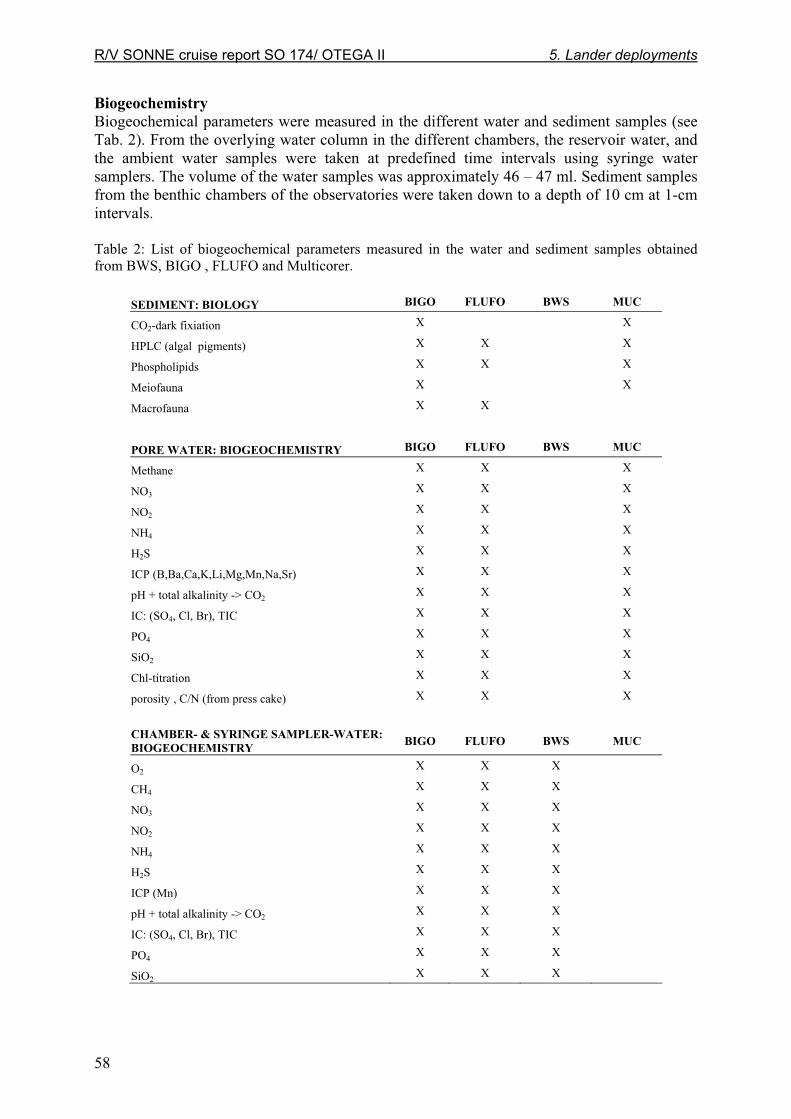
R/V SONNE cruise report SO 174/ OTEGA II 5. Lander deployments
58
Biogeochemistry
Biogeochemical parameters were measured in the different water and sediment samples (see Tab. 2). From the overlying water column in the different chambers, the reservoir water, and the ambient water samples were taken at predefined time intervals using syringe water samplers. The volume of the water samples was approximately 46 – 47 ml. Sediment samples from the benthic chambers of the observatories were taken down to a depth of 10 cm at 1-cm intervals. Table 2: List of biogeochemical parameters measured in the water and sediment samples obtained from BWS, BIGO , FLUFO and Multicorer.
SEDIMENT: BIOLOGY BIGO FLUFO BWS MUC
CO2-dark fixiation X X
HPLC (algal pigments) X X X
Phospholipids X X X
Meiofauna X X
Macrofauna X X
PORE WATER: BIOGEOCHEMISTRY BIGO FLUFO BWS MUC
Methane X X X
NO3 X X X
NO2 X X X
NH4 X X X
H2S X X X
ICP (B,Ba,Ca,K,Li,Mg,Mn,Na,Sr) X X X
pH + total alkalinity -> CO2 X X X
IC: (SO4, Cl, Br), TIC X X X
PO4 X X X
SiO2 X X X
Chl-titration X X X
porosity , C/N (from press cake) X X X
CHAMBER- & SYRINGE SAMPLER-WATER:
BIOGEOCHEMISTRY BIGO FLUFO BWS MUC
O2 X X X
CH4 X X X
NO3 X X X
NO2 X X X
NH4 X X X
H2S X X X
ICP (Mn) X X X
pH + total alkalinity -> CO2 X X X
IC: (SO4, Cl, Br), TIC X X X
PO4 X X X
SiO2 X X X

R/V SONNE cruise report SO 174/ OTEGA II 5. Lander deployments
59
Oxygen: Oxygen concentrations of the water samples were fixed immediately after retrieval of the gears. The concentrations were determined soon after retrieval using automated Winkler titration. The samples were stored for 8 hours at most.
Methane: From the water samples, 10-ml-subsamples were transferred into 20-ml gas tight
reaction vessels for headspace analyses. These vials contained 6 ml of saturated NaCl solution with 1.5 gr of excess NaCl to avoid dilution after addition of the water sample. Sediment samples (1 cm-3) for methane determination were suspended in headspace vials (20 ml) containing 5 ml of NaOH in saturated saltwater. Methane concentration was determined within 48 hours using a Shimadzu GC14A gas chromatograph equipped with FID. Prior to the analyses the samples were equilibrated for at least 2 hours in an overhead shaker.
Bioirrigation/ Transport processes: To determine bioirrigational activity during deployments
of BIGO and FLUFO bromide (7.24 g) was injected into the chambers 10 min after they had been pushed into the sediment. Bromide concentrations will be determined using ion chromatography.
Chlorophyll a: Sediment samples for the determination of chl.a and pheopigment
concentrations were taken, they serve as an indicator for the input of phytoplankton derived Corg. Analyses will be conducted in the home laboratory using the HPLC technique.
CO2 dark fixation: This parameter provides a measure of the non-photosynthetic endogeneous
production of POC in the sediment, chemoheterotrophic and chemoautotrophic 14CO2 uptake into sediment particulate organic matter was analysed as described by Sommer et al. (2002).
Meiobenthos/ Makrobenthos: These samples were taken for analysis of their taxonomic
composition, abundance, biomass. From selected samples the 13C/12C isotopic composition will be determined to assess their position within the chemosynthetically based food web and their contribution to the gas hydrate derived carbon transfer within the benthic community.
Phospholipids, PL: PL will be determined as biomass parameter of the small-sized benthic
community comprising fungi, bacteria, protozoans and metazoan meiofauna. PL will be measured following the method described by Boetius and Lochte. (2000).
Pore water chemistry: Analyses of pore water chemistry (parameter, see Table 1) were
conducted according to standard methods described on the GEOMAR homepage (http://www.geomar.de/zd/labs/labore_umwelt/Meth_englisch.html).
At present, analyses of most of the biogeochemical parameters of the samples are still in progress, thus this report will mainly focus on oxygen, methane (raw data) and pH determined in the water samples obtained from BIGO, FLUFO and BWS. Deployment of the BWS allowed a high resolution of oxygen and methane concentrations in the water column from the sediment surface to 80 cm above the sea floor. In spite of a high variability vertically and between stations, oxygen concentrations displayed clear gradients at all sites, with concentrations about 30 μmol.l-1 lower at the sediment surface than about 80 cm above it (Figure 41a). Distinct differences between mat sites and reference sites were not revealed. At bacterial mat sites elevated methane concentrations were detected directly above the sediment

R/V SONNE cruise report SO 174/ OTEGA II 5. Lander deployments
60
surface, which gradually decrease with distance from the sea floor (Figure 41b,c). During BWS deployment #3 distinct peaks of highly elevated methane concentrations of about 500 ppmV were found 8 cm and between 20 – 30 cm above the sediment surface. Above bacterial mats pH appeared to be slightly higher than above the reference sediment, Figure 41d.
a
0
10
20
30
40
50
60
70
80
140 180
oxygen [μmol.l-1]
Ref.
B. Mat
b
0
10
20
30
40
50
60
70
80
0 5 10
methane (ppmV)
Ref.
#4 OB
#2 WB
0
10
20
30
40
50
60
70
80
0 200 400 600
methane (ppmV)
Ref.
#3 WB
#1 WB
c
0
10
20
30
40
50
60
70
80
7,75 7,80 7,85 7,90 7,95
pH
Ref.
B. Mat
d
Fig 41 a-d: a: Oxygen; b, c. methane; d: pH distribution in the water column up to 78 cm above the sediment surface. Ref: reference site; B. Mat: Bacterial mat; OB: mat of orange Beggiatoa; WB: mat of white Beggiatoa.

R/V SONNE cruise report SO 174/ OTEGA II 5. Lander deployments
61
On-site work
Microbial mat sites affected by shallow gas hydrates in the Gulf of Mexico displayed high spatial variability even on a centimeter scale. A clear zonation of the different chemosynthetically based faunal assemblages as had been observed at Hydrate Ridge (Sahling et al. 2002, Sommer et al. 2002, Suess et al. 1999) was not discerned. Due to this variability the distribution and coverage of different microbial mats (Thiotrix, orange and white Beggiatoa) on the sediments enclosed by the benthic chambers of BIGO and FLUFO varied considerably. Thus, replication of these measurements was difficult, rendering each chamber a particular meso-environment with its own biogeochemical signature. During some deployments the silicone membranes of BIGO's gas exchange system were heavily affected by oil, which was released from the sea floor during the measurements. This impeded the gas exchange between the chamber and reservoir. However, during the entire deployment of BIGO #2 at a bacterial mat site of white Beggiatoa the exchange system worked properly, Figure 42a-c.
BIGO #2 white Beggiatoa
0
50
100
150
200
250
300
350
0 10 20 30 40
time (h)
control
Kieme
reservoir
Bodenw.
a
BIGO #2 white Beggiatoa
0
50
100
150
200
250
300
350
400
0 10 20 30 40
time (h)
control
Kieme
reservoir
Bodenw.
b
BIGO #2 white Beggiatoa
7,60
7,65
7,70
7,75
7,80
7,85
7,90
7,95
8,00
8,05
0 10 20 30 40
time (h)
control
Kieme
reservoir
Bodenw.
c Fig. 42a-c: Temporal gradients of a: oxygen, b: methane and c: pH measured in the overlying water column inside the exchange-, control chamber, the reservoir and the surrounding bottom water during deployment of BIGO #2. In the control chamber oxygen was rapidly consumed within 30 hours corresponding to a total oxygen uptake rate of 21.0 mmol.m-2.d-1. In the exchange chamber the oxygen concentration remained stable at the outside oxygen level. The oxygen demand of the enclosed benthic community was covered from the reservoir where the oxygen concentrations strongly decreased. Total oxygen uptake in the exchange chamber was 89.2 mmol.m-2.d-1. A higher oxygen uptake in the exchange chamber, 4.2 times that of the control chamber, is linked to

R/V SONNE cruise report SO 174/ OTEGA II 5. Lander deployments
62
much denser microbial mats in the exchange chamber. Although not for extended periods of time, flux determinations were also possible during the other BIGO deployments due to the high oxygen concentration in the bottom water of approximately 150 μmol.l-1. The same applies to FLUFO's “back up chamber”. This chamber was not used for fluid- and gas flux measurements, it represents a closed system similar to the control chamber deployed in BIGO. In total we obtained complete data sets from 9 benthic chamber measurements at microbial mat locations and 3 from a reference site. Bottom time of the different deployments of BIGO varied between 23 – 63 hours and those of FLUFO between 47 – 69 hours. In sediments covered with bacterial mats the total oxygen uptake of the enclosed sediment community varied between 3.9 mmol.m-2.d-1 in sediments only covered with a few very small “tufts” of orange Beggiatoa (FLUFO #3) to 89.2 mmol.m-2.d-1 in sediments almost completely and densely covered with white Beggiatoa (BIGO #2). The average total oxygen uptake of sediments at the reference site was 3.9 mmol.m-2.d-1 (SD: 2.4; n: 3). It appears that at microbial mat sites the methane efflux from the sediment varies reflecting the different degree by which the sediment is covered with microbial mats and the variability of the total oxygen uptake rates at the different locations. Measurements made during BIGO #2 at a white Beggiatoa mat site indicate that oxygen availability exerts a certain control on the methane release from the sea floor (Figure 43). At the reference sites no efflux of methane was observed.
BIGO #2 white Beggiatoa
0
50
100
150
200
250
300
350
400
0 50 100 150 200
oxygen (μmol.l-1)
exchange ch.
control ch.
Fig. 43: Methane concentration plotted against the oxygen content of the overlying water column inside the control and exchange chamber during deployment of BIGO #2 at a bacterial mat. First results
BIGO and FLUFO allowed reliable flux measurements. First interpretations of the oxygen and methane database indicate that the availability of oxygen exerts an influence on rates of methane release from the sea floor into the water column. This may be due to a direct effect via the bacterial aerobic oxidation of methane within the oxic sediment-water boundary layer or an indirect effect on the re-oxidation of alternative electron acceptors used to sustain anaerobic oxidation processes within the sediment. Although during some BIGO deployments oil release hampered the gas exchange, the gas exchange system is essential to provide flux measurements under “natural” conditions. Due to the fast depletion of electron acceptors, benthic chamber measurements in active sediments will become artificial after a certain period of time, rendering the rate measurements questionable. By preventing severe oxygen depletion, BIGO allows to investigate benthic processes under “natural” conditions. BIGO

R/V SONNE cruise report SO 174/ OTEGA II 5. Lander deployments
63
further allows manipulation of the enclosed sediment under controlled conditions, enabling the investigation of the kinetics of benthic processes in situ. This is of particular importance to understand the potential capability of marine habitats and to assess their response to changing environmental conditions. BIGO represents an important technological step from static measurements towards a dynamic experimental platform. The determination of flux rates of solutes across the sediment-water interface is usually carried out either by direct measurements using benthic chambers or indirectly by modelling vertical concentration gradients within the sediment. High-resolution measurements in the water column can contribute substantially to rendering these determinations more robust. The newly designed BWS appears to be a promising tool for these measurements providing a very good vertical resolution at a centimeter scale. During the deployments online video control of the water sampling lance and the surroundings ensured high-quality undisturbed water samples. To enable highly undisturbed sampling in future, it is necessary to mount the sampling ports in a streamline-shaped housing, which can be directed into the current. To assure that water samples will be taken from the same “water column package” moving above the sediment, it is further necessary to collect the water samples synchronously. During our deployments of the BWS there was a time lag of about 90 seconds between the first sample and the last sample taken. Assuming a bottom current of about 20 cm.s-1 the first sample would have been taken from a water package which is located approximately 18 m further downstream when the last sample is taken. First results indicate that the deployments of the novel observatories and the BWS contribute to a more robust database of benthic fluxes in gas hydrate-bearing sediments, their spatial and temporal variability under “natural” conditions. 5.3 Deep-sea Observation System (DOS)
Peter Linke, Michael Poser, Martin Pieper, Marco Rohleder, Wolfgang Queisser and Torsten Schott
Bottom water currents with changes in velocity and direction as well as fluctuations in hydrostatic pressure due to tidal or meteorological influences are expected to have an impact on the exchange processes and biological interactions at the sediment/water inface and the distribution of gas flares expelled from active seep sites into the water column. To monitor these oceanographic control parameters in combination with megabenthic biological activity the Deep-sea Observation system (DOS) was deployed.
The DOS Lander system (Figure 44) was equipped with 2 major modules: an acoustic module with a long-ranging acoustic doppler current profiler (up-looking 75 kHz kHz ADCP, RD-Instruments) and a 3 axis MAVS current meter (NOBSKA), and an optical module with a stereo still camera and flash (BENTHOS). The DOS Lander was deployed and recovered 3 times during SO 174/1. At the end of leg 1 it was deployed for a long-term deployment at GC415 and recovered on the second leg. During the deployments the camera system was programmed to obtain stereo photographs of the seafloor area beneath the lander in 30-min intervals. The ADCP data from the deployment will be processed at GEOMAR with Mathlab routines and merged with other data sets obtained during this cruise. The photographic material from the 4 deployments will be developed and analyzed at GEOMAR. The images will be scanned,

R/V SONNE cruise report SO 174/ OTEGA II 5. Lander deployments
64
digitized and merged to a time-lapsed video to detect changes in the faunal distribution and activity during the deployment.
Fig. 44: Recovery of the DOS lander system equipped with the long-ranging ADCP (on top) and the MAVS current meter and Camera system (below).
5.4 GasQuant
Peter Linke, Michael Poser, Martin Pieper, Marco Rohleder, Wolfgang Queisser and Torsten Schott
The emission of free gas bubbles is considered as a very mechanism transporting methane from the sediment into the water column. Because of their rapid upward migration methane in the the form of bubbles cannot be consumed immediately by bacteria in the sediments and at the sediment-water interface. Thus most of the bubble-emitted gas dissolves in the water column. To quantify the volume discharged in the form of bubbles, a new hydroacoustic system was developed within LOTUS in close cooperation with ELAC-Nautik in Kiel. This system is based on a 'normal' but pressure-resistant swath bathymetry transducer that works in a horizontal direction and detects bubbles by the backscattered acoustic signal (Figure 45). This system, known as GasQuant, is deployed by a lander and can be accurately placed in front of known bubble sites to investigate the periodicity and the amount of gas rising from the seafloor for more than one week.
Fig. 45: Scheme of the GasQuant System detecting two bubble sites by the back scattered signal.

R/V SONNE cruise report SO 174/ OTEGA II 5. Lander deployments
65
GasQuant is an autonomous system composed of a newly designed pressure-resistant (100 bar) 180 kHz swath transducer (75° opening angle with 21 beams; resolution of each beam 3° horizontal and 1.5° vertical), an electronic transducer unit (SEE 30; Transmitting and Receiving Unit), a data acquisition PC, and four deep sea batteries for power supply. The transducer is fixed in a frame at the upper buoyancy circle of the lander. The SEE 30 and the data acquisition PC are both stored in a titanium barrel (40 in diameter and 80 cm long; Figure 46c) that is fixed at the tool-frame of the lander. The four deep-sea batteries with 230 Ah and 12 V each are fixed next to this titanium barrel. The SEE 30 was modified to run with batteries in a low power mode (several high power capacitors were removed). The data acquisition PC is a common micro-computer (Windows NT), which controls the system and records the data via the Hydrostar Online software of ELAC-Nautik. Special software was written to restart the computer and the entire system if the PC crashes or the SEE stops unnoticed.
A
B
C
Fig. 46:A) View of the GasQuant Lander with launcher on top ready for deployment. The tool frame at the base of the lander carries four deep sea batteries and the SEE electronics in a titanium barrel. A compass, monitored by one of the two launcher cameras, was used to control the orientation of the lander during the deployment. B) The pressure-resistant 180-kHz transducer of the GasQuant system fixed in a cardanic frame. C) The titanium barrel and the SEE 30 control and data acquisition unit. The GasQuant system was successfully deployed at Bush Hill and GC234 (Tab. 3) after extensive flare imaging surveys had been performed and revealed several targets for the deployment. Table 3: Positions of the two GasQuant deployments Station Date / Time Position Heading Site GQ 1 # 11.10.03 19:37 /
14.10.03 15:04 27°46.948 N / 91°30.478 E
north Bush Hill
GQ 2 # 17.10 03 23:36 / 20.10.03 22:38
27°44.798 N/ 91°13.300
west GC234

R/V SONNE cruise report SO 174/ OTEGA II 5. Lander deployments
66
Fig. 47: Bottom-rooted flare at Bush Hill which was chosen as a target for the GQ1 deployment. Even if the Hydrostar Online program or the Windows NT system crashed during the deployment, the entire system started again and recorded more than 2.6 GB of data in total. The raw data have to be converted and the algorithms for this purposemust be fine-tuned in order to detect and quantify the amount of free gas. This task has not yet been completed and thus no results can be shown here. 5.5 HDSD lander
Warner Brückmann, Peter Linke, Matthias Türk and Michael Poser Gas hydrate is a dynamic reservoir in the marine carbon cycle and periodically a large and focussed source of methane probably constituting the largest carbon reservoir on earth. An important topic in gas hydrate research is therefore the need for better tools to remotely estimate the volume and stability conditions of marine gas hydrate in the near subsurface. Improving these estimates is also of critical importance for determining the global and local carbon budget. It is also crucial to precisely determine the P/T conditions in the near subsurface, where gas hydrates are at the edge of their stability field. During SO 174 with R/V SONNE the HDSD tool for in-situ characterization of gas hydrates was deployed and tested for the second time. The HDSD (Hydrate Detection and Stability Determination) is designed to identify and quantify small volumes of near-surface gas hydrate through continuous in-situ thermal and resistivity monitoring in a defined volume of sediment while the sediment is slowly heated to destabilize gas hydrates embedded in it. A prototype HDSD I device with a penetration of 30 cm was used during SO 165 in 2002, an extended version of the instrument (HDSD II) with a penetration of 100 cm was built subsequently and deployed during cruise SO 174. In the SFB working area off Costa Rica we were faced with the problem that known occurences of gas hydrates were of very minor volume. Yet their impact had to be considered in carbon budget calculations and their dilution, i.e. their freshening effect, in analyses of pore waters composition. Therefore a means for determining small volumes of gas hydrates was needed to better constrain their occurence in mud diapirs in the SFB working area. Furthermore, a tool is needed to get ground truth of different theoretical hydrate stability models (Skoan 1998) which show considerable variabilty in defining PT stability curves for any given gas composition. As the amount of energy needed to mobilize and extract gas from

R/V SONNE cruise report SO 174/ OTEGA II 5. Lander deployments
67
gas hydrate, especially under in situ conditions, is only tentatively known a tool is needed to determine these basic parameters. Although there are other means of physically detecting gas hydrate occurrences such as seismic imaging of the BSR (deep) or surveying for vent faunas (shallow), they are usually not capable of quantifying gas hydrate deposits. Frequently, a thin sediment cover prevents direct observation, and coring of hydrate-bearing sediments recovers only the largest pieces of gas hydrate that withstand rapid decay during and after recovery. To sufficiently address all these issues the Hydrate Detection and Stability Determination (HDSD) tool was developed as part of the SFB 574 subproject B2. The primary goal of identifying and quantifying near-surface hydrate layers was to be achieved through focussed heating to locally destabilize hydrate and monitor this process through continuous thermal and electrical resistivity profiling. HDSD II
To address the technical issues encountered during the two initial trials, several major improvements were necessary. The geometry of heating and sensor was completely changed to provide a more efficient energy transfer to the sediment, and the penetration depth was extended to 100 cm. In the new HDSD II design three parallel stingers are slowly pushed into the sediment to a depth of 100 cm (Figs.48-50). One stinger is heated over the entire length to produce a radial thermal field. Two sensor stingers at different distances from the heating lance are equipped with 23 temperature and resistivity sensors each 4 cm apart (Figure 48). In this configuration the heat field radially expanding from the heating lance is monitored from the sediment-water interface down to 100 cmbsf. This new geometry greatly improves the rate of heat transfer to greater depth and reduces the duration of the experiment, both factors increasing the chances of detecting hydrates. The three stingers are connected by a guiding ring 5 cm above their tips to maintain a precisely defined distance between heat source and sensors (Figure48). The control and data acquisition unit for HDSD was completely redesigned and is now based on a miniaturized industry standard PC which is programmed and controlled by a BASIC program. Data acquisition and control units are housed in a pressure vessel, the unit can be accessed via a serial RS232 interface by a standard PC keyboard and monitor for programming and data download.

R/V SONNE cruise report SO 174/ OTEGA II 5. Lander deployments
68
Fig. 48: Deployment of HDSD-II, schematic overview of tool components.

R/V SONNE cruise report SO 174/ OTEGA II 5. Lander deployments
69
Fig. 49: Sketch of the deployment of a HDSD-II-equipped lander.
Fig. 50: Photos of HDSD deployment and tool details. HDSD II was deployed during R/V SONNE cruise SO 174 (OTEGA II) to the Gulf of Mexico which was primarily focused on gas hydrate research on the Texas/Louisiana continental shelf. The main working areas were the Bush Hill and the Green Canyon complexes (GC415 lease block), which are characterized by an association of hydrocarbon seeps, gas hydrates, and chemosynthetic communities occuring at water depths of 500 m (Bush Hill) and 1000 m (GC415). Three deployments were carried out during the cruise, one

R/V SONNE cruise report SO 174/ OTEGA II 5. Lander deployments
70
of which did not yield useful data due to a shutdown shallow in the subsurface while the other two deployments were successful in collecting a complete set of temperature data, but no resistivity measurements. First deployment at Bush Hill (Station 75, HDSD-1)- due to an excess power consumption shallow in the sediment section the emergency shutdown was activated and no data collected. A second deployment (Station 92-2, HDSD-2) took place in the Bush Hill working area at a water depth of 500 m on a bacterial mat site indicating the presence of shallow gas hydrates. Here the complete heating and measurement program was carried out, including a 20-h heating cycle. Temperature measurements in both stingers were successful, while the sensors for electrical resistivity profiling failed, possibly due to highly saline pore water in superficial sediments, exceeding the measurement range of the resistivity sensors by far. Another possible reason for poor resistivity data could be galvanic contact between sensors and deep-sea batteries used in the deployment. This problem was addressed by switching to a different battery system mounted remotely on the lander frame. The third deployment (Station 151, HDSD-3) took place in the GC415 working area above an extensive bacterial mat at site GC415 at a water depth of 1000 m. The stinger array penetrated the the sediment to a depth of 80 cm, as was visually documented by an automatic underwater camera. Due to the tight time schedule of the cruise the deployment parameters and program for 49 hours after deloyment read as follows:
waiting state 3 hours penetration 1 hour thermal equilibration 4 hours heating phase I (16°C) 12 hours heating phase II (25°C) 6 hours thermal re-equilibration 10 hours retraction of stingers 1 hour
Upon recovery of the HDSD the data collected were successfully downloaded from the tool. With the exception of the uppermost three sensors all sensors had penetrated the sediment and collected 1467 individual temprature measurements, a total of about 31000 data per stinger, while no resistivity measurements were collected. The reason for the failure of the resistivity sensors is yet unknown. Due to the reasons given above the third deployment of the HDSD II can be best evaluated in terms of gas hydrate detection. Near the site of deployment we recovered a 2-m-long gravity core, which showed several layers of gas hydrate at depths between 30 and 50 cm, so the HDSD data have to be scrutinized for hydrate occurences at similar depths. At the time of writing – just hours after recovery of the tool – it is not possible to completely evaluate all details of this data set, however, the most intriguing features are obvious. For a first overview of all available temperature data, all sensor data from stingers L1, L2, and L3 are shown and annotated vs. time (Figure 51). The smooth equilibration phase testifies that all sensors were working properly. It is immediately evident that the near field sensors of L1 and the far field sensors of L2 both show a clear response to both heating cycles carried out during the experiment. While the three topmost sensors above or at the sediment-water interface are not taken into account, all temperature profiles below 20 cmbsf in L1 and L2

R/V SONNE cruise report SO 174/ OTEGA II 5. Lander deployments
71
Fig. 51: Overview of first results of the HDSD II deployment during SO 174. Please refer to the text for details.
show very regular trends of increasing temperatures with time in response to both heating increments. Although the temperature increase with time is becoming more pronounced with depth it is clear from the continuous trend that no gas hydrate dissociation was achieved. Even though the L1 near field sensors below 50 cmbsf show an increase of 8°C compared to the initial temperature of 5°C at the end of the second heating phase, extrapolation of temperature curves shows that this was still about 2°C below a steady state situation.

R/V SONNE cruise report SO 174/ OTEGA II 5. Lander deployments
72
A more complex temperature pattern is seen directly at the heating stinger L3. These measurements exhibit high frequency variations that reflect the cyclic heating-cooling control and regulation pattern. This is most clearly seen in the uppermost part of L3. While heating energy is provided uniformly to the whole length of L3, the temperatures never seem to reach the predetermined threshold of 16°C or 25°C especially in the shallower parts near the surface. This effect is more clearly seen in a direct comparison of L3, L2, and L1 temperatures in three selected intervals at the deepest part (Figure 52) and the the shallowest part of the tool. Figure 52 a-c shows a textbook-like behavior of heating and response in the lowermost part, while Figure 53 a-c shows that almost none of the energy provided by L3 reaches L1 or L2. This is an important observation as it indicates that between 4 and 16 cmbsf L1 and L2 appear to be insulated from the heat front. It is known from other experiments in this area that gas hydrate is a very effective thermal insulator. MacDonald et al. show that short-term fluctuations of bottom water temperature are not reflected in the temperature a few centimeters within massive gas hydrate deposits.
Fig. 52: Temperature data from the lower sensors #15 (= 48 cmbsf, A), #20 (= 68 cmbsf, B), #23 (= 80 cmbsf, C) for all three sensor stingers.

R/V SONNE cruise report SO 174/ OTEGA II 5. Lander deployments
73
As a first assessment of the results of this test we are concluding that the observed pattern of apparent thermal insulation in the shallowest part of the penetrated sediment section is reflecting a layer of hydrate about 12 cm in thickness, a result entirely within the observed range of hydrate occurences in the area known from other sampling and observation tools such as MUC (multicorer) or MAK (Multi Autoclave Corer). Although this conclusion is reached through an effect different from the original concept of the HDSD tool, which was based on progressive destabilization of hydrate, this thermal perturbation experiment has proved to be useful in detecting shallow gas hydrate.
Fig. 53: Temperature data from the lower sensors #15 (= 48 cmbsf, A), #20 (= 68 cmbsf, B), #23 (= 80 cmbsf, C) for all three sensor stingers.

R/V SONNE cruise report SO 174/ OTEGA II 6. Sediment sampling and sedimentology
74
6. SEDIMENT SAMPLING AND SEDIMENTOLOGY
6.1 Geological sampling equipment
Friedrich Abegg, Asmus Petersen, Torsten Schott and Wolfgang Queisser Sampling for standard geological, geochemical and microbiological investigations was performed with three standard tools. For a description of the pressure coring tools see chapter 6.2. The TV-guided grab sampler is a tool located permanently onboard RV SONNE. Providing either color or black and white video signals from the seafloor, it allows to choose a well-defined position for its deployment. The video signal is transmitted via a LWL cable and is displayed online onboard the ship. The grab function is also controlled through a deck unit located in the lab, but the power for the hydraulics and the underwater lights is provided by two deep sea batteries, which limits the operation time of the TV-grab. When the desired sampling spot has been found with the video system, the tool is deployed on the seafloor by the winch and the ‘close’ button has to be pressed. Depending on the material sampled, the maximum volume to be recovered is approximately 0.8 m3. With regard to sampling gas hydrate, this tool can provide large amounts of samples (e.g. Station 157-2, TVG 10), but due to the operation procedure these samples are neither oriented within their sedimentary matrix nor pressurized. Tab. 4a shows a list of the TV-Grab deployments. Table 4a: List of TV-Grab stations. Instr. No. Stat. No. Area Lat. / Long. Depth (m) Recovery TVG 1 23 Bush Hill 27°46.94/91°30.51 584 mud, carbonate, tube worms TVG 2 56 GC234 27°44.77/91°13.31 549 mud, carbonates TVG 3 96 GC415 27°32.61/90°59.55 1049 dispersed GH, mud, oil TVG 4 105 Bush Hill 27°46.92/91°30.47 547 mud, carbonate, gas TVG 5 136 CK 2155 21°53.94/93°26.15 2915 lumps of tar TVG 6 140 CK 2155 21°54.00/93°26.4 2902 GH, carbonate, mud, oil TVG 7 143-1 Mex. Shelf 22°05.79/92°08.35 123 relict shore lines TVG 8 143-2 Mex. Shelf 22°04.86/92°08.17 116 relict shore lines TVG 9 157-1 Bush Hill 27°46.95/91°30.46 547 mud, carbonate, oil, dispersed GH TVG 10 157-2 Bush Hill 27°46.97/91°30.47 547 lots of GH, mud, oil, carbonate TVG 11 163 GC415 27°33.48/90°58.86 951 mud, carbonate dispersed GH TVG 12 169 GC415 27°33.47/9058.85 951 mud, carbonate dispersed GH The second tool used was the gravity corer. Equipped with a weight of 1.8 tons, it was used with core barrels of several different lengths. Core recovery varied between zero penetration due to large amounts of carbonate in the shallow subseafloor and 3.8 m (St. 95-2 GC 11). Instead of the standard PVC liner, a thin plastic sleeve liner was used. This allows rapid access to the material sampled, especially to the gas hydrate. An advantage of the gravity corer is that the samples are well oriented, but in most cases the soft sediment surface is lost due to the core catcher and the horizontal position of the corer on deck during core recovery. Samples from the gravity cores have mostly been used for geochemical analyses (see chapter 7). Only very few samples of massive gas hydrate could be recovered from gravity cores. In addition to the investigations of the HDSD system (see chapter 5.7) the gravity corer has been equipped with thermistor sensors. Deployments of this combination are indicated by ‘TGC’ in the station list and the following table 4b.

R/V SONNE cruise report SO 174/ OTEGA II 6. Sediment sampling and sedimentology
75
Table 4b: List of Gravity Corer and Thermistor-Gravity Corer stations.
Instr. No. Stat. No. Area Lat. / Long. Depth (m) Recovery
GC 1 47-1 Bush Hill 27°46.95/91°30.44 548 no recovery GC 2 47-2 Bush Hill 27°46.95/91°30.44 547 mud, oil GH GC 3 69-1 GC234 27°44.76/91°13.31 548 no recovery GC 4 69-2 GC234 27°44.77/91°13.36 548 mud, few carbonates GC 5 89-1 Bush Hill 27°46.95/91°30.48 550 GC 6 89-2 Bush Hill 27°46.95/91°30.47 548 GC 7 89-3 Bush Hill 27°46.96/91°30.46 544 GC 8 89-4 Bush Hill 27°46.98/91°30.47 553 GC 9 89-5 Bush Hill 27°46.95/91°30.51 554 GC 10 95-1 GC415 27°32.61/90°59.56 1044 stuck in carb. GC 11 95-2 GC415 27°32.56/90°59.56 1042 mud, oil, GH carbonates, TGC 1 150 GC415 27°32.61/90°59.54 1045 mud, oil, GH TGC 2 165 GC415 27°32.57/90°59.62 1060 TGC 3 171 GC415 27°33.48/90°58.86 953 Table 5: List of TV-MUC stations.
Instr. No. Stat. No. Area Lat. / Long. Depth (m) Recovery
TVMUC 1 7-1 Bush Hill 27°46.96/91°30.77 601 disturbed, disposed TVMUC 2 7-2 Bush Hill 27°46.97/91°30.76 602 5 cores TVMUC 3 8-1 Bush Hill 27°46.91/91°30.64 549 5 cores, disposed TVMUC 4 8-2 Bush Hill 27°46.22/91°30.48 552 6 cores TVMUC 5 18-1 Bush Hill 27°46.95/91°30.51 548 no release TVMUC 6 18-2 Bush Hill 27°46.95/91°30.54 550 6 cores TVMUC 7 19-1 Bush Hill 27°46.93/91°30.47 553 no release TVMUC 8 19-2 Bush Hill 27°46.94/91°30.46 547 no release TVMUC 9 38-1 Bush Hill 27°46.90/91°30.51 549 no release TVMUC 10 38-2 Bush Hill 27°46.93/91°30.48 547 6 cores TVMUC 11 55 GC234 27°44.71/91°13.27 569 5 cores TVMUC 12 68 GC234 27°44.76/91°13.36 543 no release TVMUC 13 87 GC234 27°44.73/91°13.33 552 6 cores TVMUC 14 110 GC234 27°40.70/91°13.33 561 5 cores TVMUC 15 132 CK 2124 21°23.69/93°23.24 2461 released in water TVMUC 16 133 CK 2124 21°23.67/93°23.10 2470 3 cores TVMUC 17 139 CK 2155 21°54.37/93°25.75 2929 4 cores TVMUC 18 156 Bush Hill 27°46.95/91°30.47 546 4 cores TVMUC 19 161 GC415 27°33.48/90°58.86 950 ? cores
An additional tool used to obtain non-pressurized seafloor samples was the multicorer. It provides high-quality cores of the uppermost 50 cm of the sediment column. Its advantage compared to the gravity corer is that the sediment surface is well preserved. This is very important for the microbiological work because bacterial mats can be recovered mostly undisturbed. For the deployments performed during this cruise the multicorer had been equipped with underwater TV. The video control is a prerequisite for choosing the desired sampling location, here mostly bacterial mats. Additionally, it allows to observe the proper function of the tool. It was used with six coring tubes, but only rarely could six cores be recovered simultaneously. Although the multicorer has been proven to be a reliable tool it did not work properly at several stations. For this reason, several parts were replaced and additionally was equipped with a system to avoid deep penetration of the frame. After these modifications there were still some malfunctions, but they were due to strong currents in the upper 200 m of the water column in the Mexican part of the Gulf. The multicorer deployments are listed in table 5.
R/V SONNE cruise report SO 174/ OTEGA II 6. Sediment sampling and sedimentology
76
6.2 Autoclave tools
Hans-Jürgen Hohnberg, Asmus Petersen and Erik Anders
The Multi Autoclave Corer (MAC) and the Dynamic Autoclave Piston Corer (DAPC) were developed with the aim of recovering, preserving and analyzing sediment cores under in-situ conditions of the deep sea. Introduction
The MAC, developed by TUB/MAT, can cut four sediment-cores from the upper sea bottom sediment layers (max. 55 cm) simultaneously at any chosen water depth. The cores can be recovered at in-situ-pressure corresponding to water depths of up to 1400 m. The MAC consists of a deployment frame with a damping system including a pull rope releaser system and eight further large structural components, namely the four coring units and the four pressure chambers. In addition, every pressure container is equipped with a pressure preserving system (accumulator) supporting the closure of the pressure chambers during the coring procedure and enabling pressure preservation over several weeks. Each of the cores is kept in a liner which is pulled into the respective pressure chamber and trapped inside in vertical direction. The MAC is deployed on the deep sea cable. When the system hits the seafloor, it is left to rest there for a certain time before being hoisted back. Function groups are activated that control the processes of coring, pulling the liner into the pressure chamber, sealing the pressure chamber and hauling under in situ pressure. Each of the four pressure chambers is enclosed by a transparent mantle tube which is filled with sea water, providing sufficient cooling of the pressure chamber. Cooling is especially vital for sediment samples that contain gas hydrate. The sediment cores can be used for various physical, chemical or biological examinations. For example, they can be scanned using non-invasive technology or they can be released from the pressure chamber for description and analysis immediately after recovery. The pressure chambers were checked and approved by the Berlin TÜV (Technischer Überwachungsverein, technical inspection authority of Germany). Stored in a safe transport box, they are suitable for transport by sea or road. The DAPC is a sediment core sampling device. Its total length is 7.2 m, its total weight 500 kg. It was designed to cut sediment cores from the seafloor surface to a maximum length of 2.3 m and preserve them at in situ pressure corresponding to water depths of up to 1500 m. Like the MAC, the DAPC is equipped with a pressure control valve allowing deployment to up to 6000 m water depth. The cutting pipe, which is relatively short (2.7 m), hits the seafloor with a very strong impact. Therefore, it is especially suitable for sampling layered, gas-hydrate-bearing sediment. The device allows various analytical approaches. Due to the novel construction of the pressure barrel, this is the first system that allows CT scanning of such cores (80 mm in diameter) in their pressurized state. The pressure barrel consists of glass-fiber reinforced plastic (GRP), aluminium alloys, seawater resistant steel and aluminium bronze. The pressure chamber is 2.6 m long and weighs about 180 kg. All parts of the pressure chamber exposed to sea water are suitable for long-term storage of cores under pressure for several weeks. The DAPC is to be deployed from a research vessel on the deep sea cable. It can be released from variable heights (1-5 m) and enters the seafloor in free fall.
Materials used
The deployment frame including the damping, releasing and coring systems consists of stainless steel (1.4571 und 1.4301), partly hot zinc dipped. The parts of the pressure chambers exposed to inner pressure were made of highly firm stainless steel (1.4462) and GRP tubes. The mantle tubes around the pressure tubes, which are exposed to tractive force, are made of a

R/V SONNE cruise report SO 174/ OTEGA II 6. Sediment sampling and sedimentology
77
highly firm aluminium alloy (AlMgSi1 F28). All materials used for the pressure chambers have been approved by the TÜV and classified by 3.1b oder 3.1a certificates. The DAPC pressure chamber is made of stainless steel (1.4571), aluminium bronze (CuAl10Ni) and a GRP pipe. The balls of both ball valves are made of 1.4404. The cutting system, consisting of a cutting-shoe and outer cutting-pipe, is made of St52. Further materials used are ball bearing steel 1.4301 and PVC.
MAC testing procedure All sediment coring tests were supported by a video telemetry system provided by GEOMAR. Different weather conditions (swell) can be compensated by changing the lowering/ hoisting speed. The different structural components are so variable that alterations are possible as a response to the test results. The following components can be adjusted during a series of tests: 1. Position of the piston within the liner. 2. Position of the sealing sleeve within the liner, determining when the water column in the
liner above the sediment surface is sealed. 3. Installation of a catching or releasing sleeve in the head of the pressure chamber, which
means an anticipatory determination of the position of the liner within the pressure tube. 4. The damping and thus the speed at which the corers enter the sediment can be adjusted by
changing the internal flow resistance. 5. The sealing characteristics of the pressure chamber immediately after the coring can be
changed by variable pre-adjustment of the initial accumulator pressure. 6. The deployment frame has adjustable feet allowing for different heights as a flexible
reaction to different types of sediment with different solidity which might affect the stability of the system.
7. The cutting force can be changed by adding more or less lead weight, which also means a change of cutting speed.
8. Installation of a core catcher. 9. 4 corers can be deployed simultaneously, so that a maximum of four different samples can
be examined and compared under identical sampling conditions. MAC tests
12 MAC-deployments were made during SO 174 (Table 6.2.1). Various combinations of the above-mentioned options were tried during the test series. Table 6: MAC deployments. Deployment No. Station Area Position at seafloor (N°;W°) Water depth (m)
MAC 1 12 Bitte einfuegen 27°44.725; 91°13.314 558 MAC 2 46-1 Nach Stationsliste 27°46.949; 91°30.453 547 MAC 3 46-2 27°46.925; 91°30.491 545 MAC 4 63 27°32.530; 90°59.595 1049 MAC 5 79 27°46.955; 91°30465 546 MAC 6 97 27°32.588; 90°59.564 1046 MAC 7 118 27°46.969; 91°30.429 552 MAC 8 141 21°54.08; 93°26.14 2929 MAC 9 152 27°32.609; 90°59.535 1041 MAC 10 158 27°46.968; 91°30.469 555 MAC 11 162 27°33.446; 90°58.861 951 MAC 12 170 27°33.452; 90°58.866 946

R/V SONNE cruise report SO 174/ OTEGA II 6. Sediment sampling and sedimentology
78
DAPC testing procedure
The video telemetry was not used for the sampling tests with the DAPC, which was released at different water depths ranging from 550 m to 1040 m. The deployment from SONNE was similar to that of normal piston corers, pushed by a weight and released by (Schere). DAPC tests
Four DAPC deployments were made during SO 174 (Table 6.2.2). Table 7: DAPC deployments. Deployment No. Station Area Position at seafloor (N°;W°) Water depth (m)
DAPC 01 90 27°46.948; 91°30.482 549 DAPC 02 149 27°32.610; 90°59.545 1039 DAPC 03 153 27°32.60; 90°59.56 1041 DAPC 04 166 27°33.474; 90°58.855 953 Stations sampled by MAC and DAPC
Station 12 (MAC1) on 9 October: LTC 4 held a pressure of almost 50 bar, LTC 2 was not under pressure for unknown reasons. A subsequent pressure test with 100 bar proved that the new flap valve and all other elements were tight. The newly constructed core/liner transfer gadget was tested for the first time using LTC 2. During the transfer, a disturbance of the sediment-filled liner caused a break of the core catcher and part of the core fell out.
Station 46-1 (MAC 2) on 13 October: The time allocated for the deployment was too short. This caused a failure of the releasing mechanism, because in the very soft sediment the relative movement between the frame and the center of the MAC was not sufficient.
Station 46-2 (MAC 3), following station 46-1: Without an intermediate recovery, the MAC system was deployed for a second try. The penetration was all right. The MAC surfaced carrying LTC 2 with 40 bar and LTC 3 without pressure. The flap valve (old flap) of LTC 3 was slightly dirty and therefore not sealed (O-ring damaged). In addition, one of the guidance was broken. Yet, the liner held 50 cm of core. A core transfer was not tried because the piston slid out of the sealing when the device was set down on board.
Station 63 (MAC 4) on 15 October: LTC 2 and 3 were deployed. LTC 3 obtained a core under pressure (75 bar). 15 liters of gas were obtained by degassing (see chapter 7.2). LTC 2 was not under pressure but contained 30 cm of core. The new flap was slanted in its fit. LTC 2 was declared unfit for use for the following deployments because its sliding sleeve got stuck so easily.
Station 79 (MAC 5) on 18 October: The MAC was deployed at a water depth of 547 m. LTC 3 and 4 were recovered without pressure. The subsequent pressure test did not reveal any fault. Sealing problems at the beginning of the pressure test indicate that the pressure adjustment (40bar) of the accumulator had been chosen too high, so that initial leakage could not be compensated. zu hoch eingestellt war und deshalb Anfangsleckagen nicht ausgeglichen werden konnten. Station 90 (DAPC 1) on 18 October. The first deployment of the DAPC was a total success with a pressure of 37 bar and a core of 1,5 m length. The accumulator pressure had been adjusted to 30 bar, the water was 547 m deep. The degassing yielded 70 liters of gas. The core was used for various studies.

R/V SONNE cruise report SO 174/ OTEGA II 6. Sediment sampling and sedimentology
79
Station 97 (MAC 6) on 19 October: LTC 3 and 4 were under pressure (75 bar). For both of them, the accumulator had been set to 50 bar at a water-depth of 1040m. Both LTCs were brought into the cooling container. The degassing of LTC 3 yielded no amount of gas worth mentioning. LTC 4 stayed inside the cooling container for later CT investigation (see chapter 6.4).
Station 118 (MAC 7) on 21 October: LTC 2 was repaired and used for this deployment. LTC 3 surfaced with a pressure of 40 bar, LTC 2 without pressure. The leakage of LTC 2 had been caused by a mounting error. The accumulator pressure had been adjusted to almost 30 bar. The water was about 550 m deep. LTC 3 stayed inside the cooling container for later CT investigation (see chapter 6.4). Station 141 (MAC 8) on 2 November: LTC 3 and LTC 4 were recovered without pressure. For both of them, the accumulator had been set to 65 bar for a water-depth of 2900m. Both LTCs contained 40 cm of core, consisting of very fine sticky clay. As the sediment structure was comparably firm and sticky in the lower parts of the cores, the pull-off force created during core transfer was so strong that one liner and both liner clamps were damaged. We assume that the damage was caused by an interaction between heaving speed (0.2 m/s), vertical ship movement, and the structure of the sediment. Station 149 (DAPC 2) on 5 November: The DAPC only maintained a slight overpressure as the lower ball valve was not completely sealed (The sealing mechanism had not been adjusted precisely). The core was used for taking samples. Station 152 (MAC 9) on 5 November: LTC 2 and LTC 4 were deployed at a depth of 1041 m with a pre-adjusted accumulator pressure of 60 bar. One LTC retrieved a pressurized core, the other LTC contained a core but was not under pressure. Non of the LTCs showed any leakages during a pressure test performed after recovery. It could not be detected why one of them had lost pressure.
Station 153 (DAPC3) on 6 November: The DAPC was recovered holding a 2-m-long core at a pressure of 80 bar. The accumulator pressure had been pre-adjusted to 60 bar for a water depth of 1041 m. Samples were taken from the core. Station 158 (MAC10) on 6 November: Both LTCs contained pressurized cores from a depth of 555 m. Before the cores underwent CT scanning, the pressure was increased to 55 bar. LTC 3 had been fitted with the alternative valve system. Station 162 (MAC11) on 7 November: Both LTCs provided pressurized cores from a depth of 951 m. The accumulator pressure had been pre-adjusted to 50 bar. Both LTCs underwent CT scanning. Station 166 (DAPC 4) on 8 November: The DAPC was recovered holding a 1.4-m-long core at a pressure of 80 bar. The accumulator pressure had been pre-adjusted to 60 bar for a water depth of 953 m. Samples were taken from the core.
Station 170 (MAC12) on 8 November: Both LTCs contained pressurized cores from a depth of 946 m (LTC1: 75 bar, LTC3: 50 bar). The accumulator pressure had been pre-adjusted to 50 bar. Before the cores underwent CT scanning, the pressure was increased to 90 bar. LTC 3 had been fitted with the alternative valve system.

R/V SONNE cruise report SO 174/ OTEGA II 6. Sediment sampling and sedimentology
80
MAC test results
Compared to leg 165-2 one year ago, core recovery and pressure stability were much better during this test series. On average, about 70% of the MAC deployment were successful in recovering pressurized cores. The improved results are due to the optimized system and the avoidance of mounting errors. Different swell conditions had no measurable influence on the deployment and recovery of the MAC. The core extraction procedure does not yet work satisfactorily using the frame that was designed for this purpose. As the core catcher has been improved, a core extraction in horizontal position without the frame appears more promising. DAPC test results
The four deployments of the DAPC were very successful. Most of the requirements for a CT scanning of DAPC cores can be met: The pressure container will have to be shortened by cutting the liner under pressure, followed by taking off the pressure container under pressure. The procedure worked in most of the details, yet the liner cutting mechanism and the liner clamping system have to be improved.
Conclusions
� The MAC tests have proven that the newly manufactured core catchers work well for LTC transport and long-term storage.
� For future MAC coring we would like to recommend extracting the core safely in a horizontal position, catching the core in two thin (2 x 0.1 mm) metal sheets arranged in a displaced position.
� The damping of the MAC frame was improved, leading to an enhanced deployment safety.
� The MAC flap valves work well, the newly constructed flap, with a slightly different inner bending, has not shown any significant advantage.
� Long-term pressure conservation works well. � The preservation of the in-situ pressure during recovery was improved by enhancements
of the sealing system that keep the volume of the pressure container constant to the greatest possible extend during the recovery procedure. After further improvements of the handling, the MAC may well become a standard system.
� The DAPC is fully functional, yet the liner cutting system has to be improved in order to allow CT scanning.
The MAC and DAPC systems were handled by H.-J. Hohnberg, Erik Anders and Asmus Petersen in very good cooperation with the deck crew.
6.3 Sedimentological results
Valentina Blinova, Thomas Naehr, Friedrich Abegg, Xiqiu Han and Manuela Drews A total of 15 gravity cores were taken on the Louisiana Slope, the northern study area of SO 174 (Tab. 4b). The cores were either taken with the standard gravity corer (GC; 12 cores) or using a modified version with attached thermistor probes called the thermistor gravity corer (TGC; 3 cores). The TV-Grab, TV-MUC, and two different pressure coring devices (TV-MAC and DAPC) were used to recover sediments, gas hydrate, and carbonate samples from both the northern and the southern study areas. Gravity coring served several purposes: sampling of long sections of gas hydrate-bearing sediments, sampling for geochemical reference studies, biogeochemical studies, and diagenetic studies.

R/V SONNE cruise report SO 174/ OTEGA II 6. Sediment sampling and sedimentology
81
To allow for rapid access to gas hydrate-bearing sedimentary sections, the gravity corer was used with flexible plastic sleeve liners that were cut open immediately after recovery. Sediment temperatures were measured on board immediately after the cores had been opened using a hand-held thermometer and provided a simple means of identifying zones of gas hydrate occurrence in the cores. Because gas hydrate-bearing sediment cores have been known to develop dangerously high levels of gas pressure upon recovery, precautions were taken to avoid injury of personnel involved in the recovery process. However, none of the cores showed signs of overpressure, allowing for a safe removal of the core cutter. After description, documentation, and sampling, the sediment cores were returned to the sea because the decomposition of gas hydrate in these cores quickly altered or destroyed primary sedimentary structures and chemical gradients, making archiving of these cores impractical. All gravity cores were taken in the northern study areas (Bush Hill and Green Canyon Site 415; Figure 54). The following is a brief description of the main textural and compositional features of these cores.
Fig. 54: Graphic representation of lithologies within the sediment cores taken during SO174.

R/V SONNE cruise report SO 174/ OTEGA II 6. Sediment sampling and sedimentology
82
Station 47-1 GC 1 and Station 47-2 GC 2
The first two gravity cores were taken in the Bush Hill area in order to recover gas hydrate-bearing sediments. The first coring attempt was only partially successful, recovering a small amount of sediment and several pieces of gas hydrate (up to 2 cm in size). GC 2 was taken at the same location and recovered 280 cm of dark gray clay (Figure 54). A strong smell of H2S was noticed. The top 90 cm consisted of hemipelagic clay and mud, with a high water content in the uppermost part. From 90-190 cm below the sea floor (cmbsf) the sediments were highly gas saturated and contained small pockets of oil. The interval from 170 to 190 cmbsf was characterized by very dry mud, followed by 90 cm (190-280 cmbsf) of a very oily, mousse-like sediment with gas hydrate. Gas hydrate pieces were up to 2 cm in size and occurred either as thin crusts or rounded concretions. Small carbonates nodules were collected from the bottom part of the core. Station 69-1 GC 3 and station 69-2 GC 4
Gravity cores GC 3 and GC 4 were taken from Green Canyon (GC) Site 234. The first coring attempt was unsuccessful and did not result in penetration of the sediment. Subsequently, GC 4 was taken at the same location and recovered 209 cm of sediment (Figure 6, core log). Dark gray foraminifera-bearing mud was recovered. Light gray pebbles of fairly stiff clay were observed throughout the core. A weak smell of H2S was noticed at 150 cmbsf. The interval from 118-125 cmbsf consisted of shell debris followed by small carbonate nodules (up to 1 cm in diameter). Minor amounts of oil only occurred at 110 and 200 cmbsf.
Stations 89-1 GC 5, 89-2 GC 6, 89-3 GC 7, 89-4 GC 8, and 89-5 GC 9
These gravity cores were taken in different parts (central and northern) of the Bush Hill area. Core 89-1 GC 5 consisted of dark gray mud, which emitted a strong smell of H2S (Figure 54). Sediments were highly water-saturated to a depth of 50 cmbsf. Shell debris with oil was collected from the interval between 25-43 cmbsf. Carbonate concretions occurred at 90, 125 and 178-220 cmbsf. Very dry sediments were noticed near the base of the core. Core GC 6 recovered dark gray homogeneous clayey sediment with a strong smell of H2S (Figure 54). Carbonates occurred at 60 cmbsf and from 126 to 129 cmbsf together with several oil pockets. Core 89-3 GC 7 is similar to the previous one (Figure 54). It is characterized by dark gray homogeneous clay, with a strong smell of H2S. Carbonates occurred at 60 cmbsf and from 126 to 129 cmbsf together with oil patches. Shell material was common from 35 to 40 cmbsf. Dark gray homogeneous clay with pebbles of more indurated light gray clay was recovered in core GC 8 (Figure 54). The sediment was characterized by a strong smell of H2S. Shell material occurred at the 30-50 cmbsf interval. Carbonates were present from 65 cmbsf to the base of the core in form of small nodules (less then 1 cm in diameter). Sediments below 170 cmbsf were very dry and oily. Only 88 cm of dark gray homogeneous clay were recovered by core GC 9 (Figure 54). The sediment was characterized by a strong smell of H2S. Carbonate nodules and shells were present from 29 to 42 cmbsf. A large, 7-cm-thick carbonate crust occurred from 60 to 68 cmbsf. Below 78 cmbsf the sediment contained a large number of small nodules and appeared to be saturated with oil. Stations 95-1 GC 10 and 95-2 GC 11
Gravity cores 10 and 11 were taken at site GC415. The first attempt was unsuccessful because the core could not penetrate the sediments, presumably due to the presence of a thick

R/V SONNE cruise report SO 174/ OTEGA II 6. Sediment sampling and sedimentology
83
carbonate crust. GC 11 was taken at the same location and recovered 380 cm of sediment (Figure 54), which consisted of dark gray clay with a strong smell of H2S. The upper 90 cm of the sediment were water saturated. Some oil as well as small carbonate nodules occurred at 130 and 158 cmbsf. From 190 to 200 cmbsf and at 380 cmbsf, the dark gray sediment exhibited a soupy, mousse-like texture indicating the presence of gas hydrate. Oil was present in pockets and a strong smell of H2S was noticeable. Carbonate nodules occurred in the same intervals. Below 270 cmbsf vertical fractures were filled with oil, but the overall appearance of the sediments was dryer. Station 150 TGC 1
The first deployment of the Thermistor Gravity Core recovered 200 cm of greenish-gray to dark gray nannofossil-rich mud from the Green Canyon site GC415 (Figure 54). The top 42 cm of the core consisted of greenish-gray mud with no apparent gas hydrate. From 5-10 cmbsf, the sediment contained a large number of small, cm-sized carbonate nodules. The following 38 cm (42-80 cmbsf) were dominated by the presence of pieces of gas hydrate that had presumably formed layers or veins in the undisturbed sediment. As in all cores from seep sites in the Gulf of Mexico, oil was present in various amounts in the sediment. Decomposition of the hydrate led to a soupy, mousse-like texture of the sediment upon retrieval. Disseminated gas hydrate was present to a depth of 140 cmbsf, but presumably in smaller amounts. Dry, dark gray sediment with characteristic scaly fabric occurred in the lowest part of the core, from 140 to 200 cmbsf. The relative dryness of the sediment below the gas hydrate-bearing interval was probably caused by desiccation during gas hydrate formation. Station 159 GC 12
Gravity core 12 from GC415 consisted of 135 cm of greenish-gray nannofossil-rich mud. The silt-sized components included quartz, sponge spicules, pyrite, and other heavy minerals. The core contained gas hydrate in varying amounts of gas hydrate throughout (Figure 54) Oil was also present throughout the core, as were very porous, sponge-like hydrate pieces that occurred in layers between 72 and 96 cmbsf.
Station 165 TGC 2
Core TGC 2, also taken at GC415, recovered 465 cm of greenish-gray nannofossil-rich mud (Figure 54). Since the core was taken with a three-meter core barrel, recovery was 155%. Sediment in excess of 3 m had been pushed into the head of the gravity corer, which was also lined with a flexible sleeve liner. The sediment contained no visible gas hydrate and lacked the typical soupy texture. The interval from 350 to 400 cmbsf was somewhat dryer than usual and oil was present from 0 to 400 cmbsf.
Station 171 TGC 3
Core TGC 3 recovered 400 cm of greenish-gray to dark gray nannofossil-rich mud (Figure 54). The top 30 cm consisted of oily greenish-gray sediment, followed by 70 cm (30-100 cmbsf) of very soupy, mousse-like sediment with abundant oil and gas hydrate (massive piece at 74 cm). Gas hydrate decomposition was also evident from very cold sediment temperatures (as low as -6.6 ºC). From 100 to 350 cm, the sediment appeared relatively dry with no apparent gas hydrate. The lowermost portion of the core (350-400 cmbsf) consisted of dark gray to black mud, indicating anoxic conditions at the time of deposition.

R/V SONNE cruise report SO 174/ OTEGA II 6. Sediment sampling and sedimentology
84
6.4 Gas hydrate and CT scanning
Friedrich Abegg and Kornelia Gräf The first gas hydrate of this cruise was recovered by the gravity corer at station 47-2 (GC 2), Bush Hill, from a water depth of 547 m. It was the second deployment of the gravity corer because during the first one (St. 47-1, GC 1) the core had been lost due to a damaged tubing. Mostly dispersed gas hydrate was found in this core down from a subseafloor depth of 2 m. 5 gas hydrate subsamples were taken and immediately preserved in liquid N2. Two of the subsamples were taken from the core catcher and could be described as massive gas hydrate of orange color (Figure 55, left). The samples taken from the core were cleaned roughly, but they still contain particles of mud and oil (Figure 55, right). The maximum size of these samples is approx. 10 x 7 x 5 cm. The dispersed gas hydrate was not subsampled because of its advanced state of dissociation after recovery. Table 8: List of gas hydrate samples preserved in liquid nitrogene. .
Stat. No. Instr. No. Area Number of sub samples
47-2 GC 2 Bush Hill 5 96 TV-G 3 GC415 7 140 TV-G 6 CK 2155 7 157-2 TV-G 10 Bush Hill Numerous specimens
TV-G 3 , Stat. 96 on site GC415, again recovered mostly dispersed gas hydrate. Nevertheless, several subsamples were preserved in liquid N2. The grab also contained a lot of oil so it could not be clearly differentiated whether the color of the gas hydrate is original or caused by oil pollution. The size of the subsamples remained below the above described maximum size of GC 2. A total of seven subsamples of gas hydrate were taken. The next set of gas hydrate samples was recovered by TV-G 6. This deployment, performed at Stat. No. 140 on Chapopote, provided gas hydrate from a water depth of more than 2900 m. The subsampled gas hydrate pieces are of a maximum size of 12 x 8x 6 cm. Again, it was not possible to determine the color because of lots of oil in the sediment. In addition to the bulk samples of gas hydrate, a set of aluminium tubes with an inner diameter of 14 mm was filled with gas hydrate. These tubes were preserved for onshore Micro-CT investigations.
Fig. 55: Gas hydrate subsamples of TV-G 10. The last but overwhelming sample of gas hydrate was taken by TV-G-10 (Stat. 157-2) on Bush Hill. The grab provided a large amount of gas hydrate. Immediately after recovery of the grab such a large number of subsamples had to be placed into the liquid N2 dewars that the
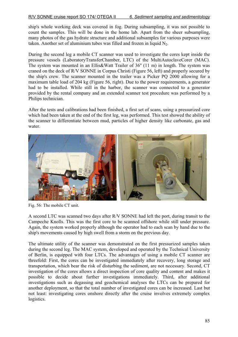
R/V SONNE cruise report SO 174/ OTEGA II 6. Sediment sampling and sedimentology
85
ship's whole working deck was covered in fog. During subsampling, it was not possible to count the samples. This will be done in the home lab. Apart from the sheer subsampling, many photos of the gas hydrate structure and additional subsamples for various purposes were taken. Another set of aluminium tubes was filled and frozen in liquid N2. During the second leg a mobile CT scanner was used to investigate the cores kept inside the pressure vessels (LaboratoryTransferChamber, LTC) of the MultiAutoclaveCorer (MAC). The system was mounted in an Ellis&Watt Trailer of 36'' (11 m) in length. The system was craned on the deck of R/V SONNE in Corpus Christi (Figure 56, left) and properly secured by the ship's crew. The scanner mounted in the trailer was a Picker PQ 2000 allowing for a maximum table load of 204 kg (Figure 56, right). Due to the power requirements, a generator had to be installed. While still in the harbor, the scanner was connected to a generator provided by the rental company and an extended scanner test procedure was performed by a Philips technician. After the tests and calibrations had been finished, a first set of scans, using a pressurized core which had been taken at the end of the first leg, was performed. This test showed the ability of the scanner to differentiate between mud, particles of higher density like carbonate, gas and water.
Fig. 56: The mobile CT unit. A second LTC was scanned two days after R/V SONNE had left the port, during transit to the Campeche Knolls. This was the first core to be scanned offshore while still under pressure. Again, the system worked properly although the operator had to each scan by hand due to the ship's movements caused by high swell from a storm on the previous day. The ultimate utility of the scanner was demonstrated on the first pressurized samples taken during the second leg. The MAC system, developed and operated by the Technical University of Berlin, is equipped with four LTCs. The advantages of using a mobile CT scanner are threefold: First, the cores can be investigated immediately after recovery, long storage and transportation, which bear the risk of disturbing the sediment, are not necessary. Second, CT investigation of the cores allows a direct inspection of core quality and content and makes it possible to decide about further investigations immediately. Third, after additional investigations such as degassing and geochemical analyses the LTCs can be prepared for another deployment, so that the total number of investigated cores can be increased. Last but not least: investigating cores onshore directly after the cruise involves extremely complex logistics.

R/V SONNE cruise report SO 174/ OTEGA II 6. Sediment sampling and sedimentology
86
Table 9: List of CT-investigated samples.
Stat. No. Instr. No. Sub sample No. Area Description No. of Slices
47-2 GC -2 1 Bush Hill GH 66 2 GH 54 4 GH 106 96 TVG-3 2 GC415 GH 53 6 GH 56 6 GH 51 97 MAC-6 GC415 LTC 132 118 MAC-7 LTC 3 Bush Hill LTC 255 136 TVG-5 Chapopete Tar 220 Shell 38 Shell 2 39 140 TVG-6 1 Chapopote GH 58 2 GH 71 3 GH 61 4 GH 47 4/1 GH 33 6 GH 59 7 GH 42 A-1 Alum. tube 12 A-2 Alum. tube 11 A-3 Alum. tube 10 A-4 Alum. tube 13 A-5 Alum. tube 14 143-2 TVG-7 P Mex. Shelf Carbonate 118 T Carbonate 116 152 MAC-9 GC415 LTC 161 157-2 TVG-10 A-1 Bush Hill Alum. tube 12 A-2 Alum. tube 12 A-3 Alum. tube 13 A-4 Alum. tube 13 A-5 Alum. tube 12 158 MAC-10 LTC 3 Bush Hill LTC 184 LTC 1 LTC 214 MAC-11 LTC 2 GC415 LTC 225 LTC 4 LTC 299 MAC-12 LTC 3 GC415 LTC 203 LTC 1 LTC 391
We were able to investigate a total of 9 LTCs on the ship. All nine LTCs were scanned under pressure and seven LTCs were used for further analyses as mentioned before. Two LTCs were placed inside a reefer container and will be scanned again when they are back in Kiel. As a first result the core overviews and some single slices have been processed. Figure 57 shows the overview of MAC 7 (Stat. 118, Bush Hill) on the left side. The core had a total length of 30 cm and the single slice (right panel) is located 20.5 cm below seafloor. This slice indicates free gas, represented by the black color inside the core. The CT scanner was also used for non-pressurized samples taken during this cruise. Inspired by its availability, several other samples were examined using the CT scanner. Among these a piece of tar, recovered from Chapopote with TVG 5, has to be mentioned. The structures of different densities visible at the surface were also observed inside the sample. Other investigations were performed on shells and pieces of carbonate, demonstrating possible applications and benefits of this tool for many purposes beyond just scanning pressurized samples. The following table provides an overview of the samples investigated with the mobile CT onboard R/V SONNE during the second leg.

R/V SONNE cruise report SO 174/ OTEGA II 6. Sediment sampling and sedimentology
87
Fig. 57: CT-images of MAC 7, left side: overview, right side: single slice.
6.5 Authigenic carbonates
Xiqiu Han, Thomas Nähr, Anton Eisenhauer and Friedrich Abegg
Authigenic carbonates were recovered with the TV-Grab (TV-G), Gravity Corer (GC), Thermistor Gravity Corer (TGC), TV-Multicorer (TV-MUC), Dynamic Autoclave Piston Corer (DAPC), and Multi-Autoclave Corer (MAC). Table 10 provides a comprehensive summary of the recovered authigenic carbonates with brief descriptions of each sample. No further on-board analyses of carbonate samples were conducted. Samples were mechanically cleaned, washed with seawater, air-dried and packaged in closed transport boxes. Authigenic carbonates recovered during SO 174 represent a geologic record of fluid venting in the Gulf of Mexico and will help constrain the geochemistry and temporal variations of fluid flow in the Gulf of Mexico region. Shore-based research will include petrographic and mineralogical description, stable isotope geochemistry, and U/Th-disequilibrium as well as 226Raexcess/Ba-method dating of selected carbonate samples. Table 10 : Summary of authigenic carbonates recovered during SO 174.
Loc./Stat. Description Notes
Bush Hill, TVG 1
Gray tabular carbonate crust. Rough surface with small pebbles, shell debris, abundant mm-sized holes; tube worms grow inside the holes. Base has bigger holes, usually 1-2 cm in size. Cross section shows the crust is composed of numerous 0.3-0.8 cm-sized pebbles; oil fills the voids.
Carbonate, tube worms
Gray massive calcareous crust, dense texture, oil in fissures. Calcareous mudstone with curved surface.
GC415, TVG 3 Carbonate crust, 2-4 cm thick, porous, abundant small pebbles, tube worms grow in the
small holes, which are filled with oil. Surface is rougher than base. Large holes also present (3x3cm, 1.5x1.5cm); channels for fluid flow?
Dispersed GH in oily mud
Bush Hill, TVG 4
Irregular carbonate crust. Pebbles (0.5-1cm in size) abundant on surface. Base contains more mud. Traces of oil and shell debris are common.
No GH observed
CK 2155, TVG 6
Gray irregular massive carbonate, large pieces, 30-60x20-30x30-40cm, porous, oil fills holes or cavities, abundant shell debris, mud clasts. not well cemented.
Dark gray, GH present
Carbonate-cemented, well-preserved clams. Oil fills cavities. Bush Hill, TVG 9 Tabular crust, 4 cm thick, rough surface, pebbles 1-2 cm in size, a white layer (aragonite?).
Bush Hill, TVG 10
Tabular concretion, usually 4-6 cm thick, some up to 10 cm. abundant shell debris and mud clasts. Oil fills pores. Elongated pebbles (2-6 mm in dia.); Some samples contain numerous, well preserved shells.
GH present

R/V SONNE cruise report SO 174/ OTEGA II 6. Sediment sampling and sedimentology
88
GC415, TVG 11
1) Irregular tubular concretions, channels connected with each other, usually 1.5-3 cm, up to 4-8 cm in dia., walls are 0.5 cm thick, some of the channels are partially filled with soft clay and oil, some are clogged. One sample has U-shape fluid channel or burrow? 2) Tabular slabs, 2-4 cm thick, with numerous holes, 0.2-0.8 cm in diameter 3) Light gray crusts, 2 cm thick; inside is gray and dense. Cavities 1 -2.5 cm in dia. Looks very different from the other samples from the same grab.
GH, oil, and greenish calcareous clay present
GC415, TVG 12
1) Tabular crust, size: 30-40 x 30-40 x 1-3 cm, rough surface. Yellowish porous surface, greenish base. 2) Irregular concretion, interlinked channel molds (1 cm in dia.).
GH, oil present
GC415, DAPC 2
Irregular tubular concretion, channel 1-2 cm in diam., 4-6 cm long. No pressure
Bush Hill, GC 2
Tabular concretion, porous, with oil, surface rich in pebbles (0.2-0.5 cm in diameter, <1 cm long), base is smoother.
GH at 2 mbsf
GC234, GC 4
Gray irregular micritic concretions. Contain mud and shells; 1x1 cm, 4x2 cm in size. no GH
Bush Hill, GC 5
Gray irregular concretions. Mainly composed of shell debris (80%), filled with brown oil. 2.2 m core
GC415, GC 11
Gray irregular calcareous concretions; micritic; tubular shape, with oil and mud inside the tube.
Bush Hill, GC 12
Irregular concretions, 1.5-6 cm in size, contain oil.
Bush Hill, MAC 7
Gray irregular calcareous crust. 0.5-1 cm thick; micritic, porous, with pebbles.
GC415, TGC 1
Gray, irregular carbonate concretions, rough surfaces; cavities 1-2 cm in dia.; Carbonate recovered from 20-22, 26, 40-42, 44-46, 46, 58,111,122,128,134-138, and 142 cmbsf.
GH below 40cmbsf, 1.8m core
0-5 cm: irregular, small carbonate concretions (1-3 cm in dia.), rough surface; contain oil. GH 5-10 cm: same as above GH 24-31 cm: same as above GH 40-50 cm: gray tubular carbonate concretion, composed of 2 parts, channel mold (2x2 cm) inside, lithified sediments outside.
GH
150 cm: dense carbonate slab, smooth surface, 0.5 cm thick.
GC415, TGC 3
276 cm: irregular tubular concretion, 1-1.5 cm in dia., 10 cm long. GC415, MUC 19
Gray massive carbonate, light gray surface, dark gray interior; dense. 2-4 cm long desiccation cracks, oil fills cracks; dolostone?
3 pieces of carbonate, GH

R/V SONNE cruise report SO 174/ OTEGA II 7. Pore water and gas investigations
89
7. PORE WATER AND GAS INVESTIGATIONS
7.1 Pore water chemistry
Manuela Drews, Sonja Kriwanek, Valentina Blinova, Anja Kähler and Laura Hmelo The bjective of the geochemistry pore water program was a geochemical characterization of gas hydrate- and oil-bearing sediments. Sampling stations were mostly chosen at gas hydrate and oil sites in the northern Gulf of Mexico on the United States continental slope (Bush Hill and Green Canyon GC 234, and GC 415). A newly discovered seep area in the southern Gulf of Mexico, called Campeche Knoll, was also sampled. Of particular interest during leg 1 was a combination of pore water geochemistry with the inspection of gas hydrate and oil bearing sediments which are covered with bacterial mats of white and orange color, mainly at Bush Hill. Sediment and water samples for geochemical analyses were taken from the chambers of the BIGO and FLUFO landers, the Bottom Water Sampler, the multicorer, the gravity corer, the Multi Autoclave Corer, and the Dynamic Autoclave Piston Corer. The primary aim of leg 2 was the pore water geochemistry of long cores, taken with the gravity corer, to investigate gas hydrate-bearing sediments at greater depths. This leg's focus was more on the investigation of gas hydrate and brine sediments in the Green Canyon and Campeche Knoll areas. We also analyzed pore water from sediments obtained by the autoclave tools, the gas composition and gas volume of which was determined after degassing (see chapter 7.2). Sediment analyses were performed on samples taken with an array of different devices. Of these, the multicorer and Multi Autoclave Corer were supplemented with video equipment for deployment control. Stations for the gravity corer and Dynamic Autoclave Piston Corer were chosen according to optical and geophysical surveys, and at sites where gas and oil vents were already known. Particular devices were the multicorer (TV-MUC), the benthic lander (BIGO) simulating ocean floor conditions, the Fluid Flux Observatory (FLUFO), the TV-guided sediment grab (TVG), and the gravity corer (GC), the latter sometimes being equipped with thermistor probes and in these cases marked "thermistor gravity corer" (TGC). Two different pressure coring devices were used, the video-guided Multi Autoclave Corer (MAC), and the Dynamic Autoclave Piston Corer (DAPC). Undisturbed surface sediment samples could be procured with the multicorers and with both landers. The gravity corer's inner tube was lined with a tubular plastic film by which the sediment core could be pulled out in less than 3 minutes after the device had been recovered. After the tube had been sliced, the core lay ready for subsampling. Spatula were used for sampling every 5 to 40 cm; the subsamples were immediately brought into the cold room for further preparation. The rapid sampling routine provided the opportunity to collect gas hydrate pieces before the sediment was taken away for pore water analyses. Pore water was squeezed from the sediment in the cold room through 0.2 μm cellulose acetate membrane filters at 4 °C and at up to 3 bar pressure applying argon gas with a mechanical polypropylene press. For pore water samples appropriate for acetate measurements, acetate-free filters were used. Sediment from the multicorer or from BIGO and FLUFO push cores was cut into slices of 1–3 cm in thickness after the sediment had been pushed out with the

R/V SONNE cruise report SO 174/ OTEGA II 7. Pore water and gas investigations
90
help of an extruder. The 60-cm-long pieces of the DAPC liner were pushed out and subsampled similarly. The types of analyses performed on the pore water are listed in Table 11. Identical methods had been applied to pore water from former cruises to Hydrate Ridge (Cruise Report SO 143, 1999; SO 148, 2000, SO 165, 2002) and the Black Sea in 2001 (Cruise Report METEOR 52-1, 2002). To avoid artifacts from outgassing of H2S during long-time storage, alkalinity and H2S concentrations were determined almost immediately after the pore water samples had been collected. Table 11: Techniques used on board for pore water analysis of freshly gained samples.
Constituent Method Reference
Hydrogen sulphide Spectrophotometry Grasshoff et al. (1983)
Alkalinity Titration Ivanenkov and Lyakhin (1978)
Ammonium Spectrophotometry Grasshoff et al. (1983)
Nitrate Cadmium Reduction Column,
Spectrophotometry
Grasshoff et al. (1983)
Silicate Spectrophotometry Grasshoff et al. (1983)
Phosphate Spectrophotometry Grasshoff et al. (1983)
Chloride Mohr (AgNO3)-Titration Gieskes et al. (1991)
7.1.1 Spectrophotometric methods
The analytical techniques used on board to determine the various dissolved components are listed in Table 11. Modifications of pore water analyses were necessary for samples with high sulphide contents (above 1 mM). In order to remove H2S from such samples, the pore water was acidified with suprapure 30 % HCl (10 μl/1 ml sample) and flushed with argon gas for 5 min until no H2S smell was detectable. The degassed samples were used to measure silicate, nitrate, and phosphate concentrations applying the standard photometric procedures after Grasshoff et al. (1983). Silicate was determined after the elimination of sulphides by applying the standard manual molybdenum blue method (Grasshoff et al., 1983). Standard photometric methods (Grasshoff et al., 1983) were also used to measure ammonium and phosphate concentrations. For nitrate determination, the pore water was diluted with ammonium chloride buffer and passed through a cadmium reductor column. These samples were either frozen until measurement or measured on board within three hours. As the copperized cadmium granules of the reductor decomposed by dissolving sulfide, only sulfide-free and acidified samples were analyzed for dissolved nitrate; the nitrate data are the sum of nitrate and nitrite concentrations. 7.1.2 Titration of chloride
If chloride is measured by titration with silver nitrate, samples with H2S concentrations of more than 1 mM must be pretreated to avoid corruption of the results by the precipitation of Ag2S. The pore water samples were diluted 1:2 with 0.1 N suprapure HNO3 and degassed overnight in the cold room in open vials to remove the H2S.

R/V SONNE cruise report SO 174/ OTEGA II 7. Pore water and gas investigations
91
7.1.3 Total alkalinity (TA)
Total alkalinity measurements were performed by direct titration of 1 ml or less pore water with 0.01 N HCl in an open cell (Ivanenkov and Lyakhin, 1978). The acid was standardized with an IAPSO seawater solution. Table 12: Number of samples taken from cores and type of analyses performed on board the ship
during SO 174 leg 1. BW: bottom water, GH: gas hydrate. The numbers for the MUC and most lander
pore water samples include bottom water samples.
Table 12: Number of samples taken from cores and type of analyses performed on board the ship
during SO 174 leg 1. BW: bottom water, GH: gas hydrate. The numbers for the MUC and most lander
pore water samples include bottom water samples.
H2S TA NH4 NO3 Cl PO4 SiO2 IC ICP acetate d13C d18O analysed No. of Remarks
Sample depth [cm] samples
BWS 1 X X X X X X X X X - - - - 4 = DOS 2
MUC 2 X X X X X X X X X - X X 46 23 reference
MUC 4 X X X X X X X X X - X X 31 18 mussels, white Beggiatoa, oil
MUC 6 X X X X X X X X X X X X 34,5 19 white bacterial mat, oil
BIGO 1 Ki X X X X X X X X X - X X 13 13 whilte bacterial mat, oil
BIGO 1 Ko X X X X X X X X X - X X 9 9 " , no BW
BIGO 1 water X X X X X X - X X - - - - 23
FLUFO 1 Real X X X X X X X X X - X X 16 13 white bacterial mat
FLUFO 1 BU X X X X X X X X X - X X 10 11 "
FLUFO 1 water X X X X X X - X X - - - - 14
BWS 2 X X X X X X - X X - - - - 14
BWS 3 X X X X X X - X X - - - - 14
BIGO 2 Ki X X X X X X X X X - X X 10 11 white bacterial mat, few orange patches
BIGO 2 Ko X X X X X X X X X - X X 13 12 white bacterial mat, gas develepment, oil
BIGO 2 water X X X X X X - X X - - - - 23
GC 2 X X X X X X X X X X X X 245 9 GH, carbonates
MAC 4 X X X X X X X X X - X X 15 13
sampling after degassing, oil, few
carbonates
GC 4 X X X X X X X X X - X X 195 9 reference
FLUFO 2 Real X X X X X X X X X - X X 10 11 white bacterial mat
FLUFO 2 BU X X X X X X X X X - X X 13 12 white bacterial mat, mussels
FLUFO 2 water X X X X X X - X X - - - - 13
BIGO 3 Ki X X X X X X X X X - X X 10 10 no BW, disturbed surface
BIGO 3 Ko X X X X X X X X X - X X 9 9 no BW, disturbed surface, oil
BIGO 3 water X X X X - X X X X - - - - 28
MUC 13 X X X X X X X X X X X X 37 20 organe bacterial mat, carbonate, gas?
GC 5 X X X - X X X X X - X X 205 10 GH, oil, carboante
GC 7 X X X - X X X X X - X X 140 8 oil, carbonate, mussel shells
GC 8 X X X - X X X X X - X X 280 9 oil carbonate, mussel shill
GC 11 X X X - X X X X X X X X 365 10 oil, carbonate
DAPC 1 X X X - X X X X X - X X 150 10sampling after degassing, bacterial mat, oil,
mussel shells, carbonate
BIGO 4 Ki X X X X X X X X X - X X 10 11 reference
BIGO 4 Ko X X X X X X X X X - X X 10 10 reference, no BW sample
BIGO 4 water X X X X - X - X X - - - - 28 reference
FLUFO 3 BU X X X X X X X X X - X X 13 12 few organe bacterial mats, site GC234
FLUFO 3 Real X X X X X X X X X - X X 13 12 very few bacterial mats
FLUFO 3 water X X X X - X - X X - - - - 14
BWS 4 X X X X - X - X X - - - - 14
BWS 5 X X X X - X - X - - - - 14
BIGO 5 K1 X X X X X X X X X - X X 12 12 reference
BIGO 5 K2 X X X X X X X X X - X X 12 11 no BW, reference
BIGO 5 water X X X X - X - X X - - - - 21 3 syringe samplers
MAC 7 X X X - X X X X X - X X 16 11sampling after degassing, gas, oil,
carbonates

R/V SONNE cruise report SO 174/ OTEGA II 7. Pore water and gas investigations
92
7.1.4 Analyses in the home laboratory
Acidified subsamples of the pore water (10 μl HCl (30 %) / 1 ml sample) were prepared for ICP analysis (atomic emission spectroscopy with inductively coupled plasma) of major cations (Na, K, Mg, Li, Ca, Sr, Ba, B, and Mn). Sulfate, bromide, and iodine concentrations will be measured by ion chromatography. Concentrations of DIC, �13C, �18O and �D are to be determined on selected subsamples in the home or an external laboratory. The remaining squeezed sediment will be used for C/N/S analysis with a Carlo Erba Element Analyser. Separate aliquots of fresh sediment will be analysed for water content and dry weight. The isotopic composition of acetate in the pore water of selected samples taken during leg 1 will be determined in a laboratory at the University of Bremen. The samples were taken by L. Hmelo (working group of K.-U. Hinrichs). Summaries on the cores including amounts of samples and geochemical analyses performed on board are given in Table 12 for leg 1 and in Table 13 for leg 2.
Table 13: Number of samples taken from cores and analyses performed on board the ship during SO
174 leg 2. BW: bottom water, GH: gas hydrate. The numbers for MUC samples include bottom water
samples.
7.1.5 Preliminary results and discussion
We sampled 4 TV-guided multicores, 6 gravity cores, 16 lander sediment samples, one MAC, and one DAPC during the first leg of the cruise, and 4 TV-guided multicorers, 4 grabs, 4 gravity cores, two MACs, and two DAPCs during the second leg. From all these the pore water was analyzed for its constituents. Selected depth profiles of chemical constituents are shown in Figures 58 to 63 and discussed here in the context of their respective sampling sites.
H2S TA NH4 NO3 Cl PO4 SiO2 IC ICP d13C d18O analysed No. of Remarks
Sample depth [cm] samples
MUC 16 X X X X X X X X X X X 27.5 17 reference
TVG 5 X X X X X X X X X X X ? 4 lumps of tar
MUC 17 X X X X X X X X X X X 34 19 sediment similar to TVG 5
TVG 6 X X X - X X X X X X X 15 12 GH, oil, carbonates
DAPC 2 X X X - X X X X X X X 164 11 carbonate, oil
TGC 1 X X X - X X X X X X X 165 7 GH, carbonate, oil
MUC 18 X X X X X X X X X X X 12.5 11 GH, little oil, bubbling sediment
TVG 10 X X X - X X X X X X X ? 5 2 GH water samples, 3 pore water samples
GC 12 X X X - X X X X X X X 125 7 GH, oil, carbonates
MAC 9 X X X - X X X X X X X 17 7 analysed after degassing, oil, carbonates
MUC 19 X X X - X X X X X X X 14 11GH, bubbling sed., oil, carbonates, 3 GH water
samples
DAPC 3 X X X - X X X X X X X 207 12analysed after degassing, homogeneous
sediment, oil
TVG 11 X X X - X X X X X X X ? 5 2 GH water samples, little GH chip, oil
TGC 2 X X X - X X X X X X X 460 12 little oil, homogeneous sediment
MAC 10 X X X - X X X X X X X 23 10analysed after degassing, homogeneous
sediment
TGC 3 X X X - X X X X X X X 395 10 GH, oil, carbonates
DAPC 4 X X X - X X X X X X X 132 10analysed after degassing, 1 bottom water
sample, oil

R/V SONNE cruise report SO 174/ OTEGA II 7. Pore water and gas investigations
93
Sediments at Bush Hill
The main sampling area during leg 1 was the gas hydrate and oil seep area at Bush Hill. All lander deployments were performed here, except FLUFO 3 which was deployed at Green Canyon site GC 234 (see below). At Bush Hill (at a water depth of about 550 m) sea floor mounds (with a diameter of about 1 to 2 m across) showed gas hydrate outcropping on their flanks. Their cap consists of a thin layer of hemipelagic mud of about 10 to 30 cm in thickness (Sassen et al., 1999). The sediment contains bacterially oxidized crude oil which is rich in aromatic compounds, free gas, dispersed gas hydrate nodules, authigenic carbonates, and H2S (summarized in Sassen et al., 1999). A complex chemosynthetic community, comprising white or orange Beggiatoa mats (for morphology see Larkin et al., 1994) on gas hydrate mounds and vestimentiferan tube worms, inhabits the Bush Hill site. At Bush Hill we sampled five gas hydrate sites (GC 2, GC 5, MUC 18, TVG 10, GC 12), all of which contained oil in different amounts. Oil was also found found at stations MUC 4, MUC 6, BIGO 1, BIGO 2, BIGO 3, GC 7, GC 8, and MAC 7, yet these samples contained no gas hydrate. Steep chloride gradients were measured at stations GC 7, GC 8 (Figure 58), and MAC 7, gradients which were slighter but still meant a chloride enrichment with depth were found at sites BIGO 3, GC 2, GC 5, and GC 12 (Figure 59). The chloride enrichment was accompanied by high ammonium concentrations at stations GC 8 (see Figure 58), MAC 7, and GC 2. Slighter ammonium gradients were found at GC 7 and GC 5. All in all, except sites BIGO 3 and GC 12, which were characterized by just a slight chloride gradient with no ammonium enrichment, chloride enrichments were found at all stations together with ammonium concentrations increasing with depth.
Sediments at Green Canyon (GC 415, GC 234)
The Green Canyon study area is part of a large belt spanning the slope of the Gulf of Mexico. It contains sea floor gas vents, oil seeps, gas hydrates, chemosynthetic communities, and subsurface oil and gas fields (Roberts and Ahron, 1994; Sassen et al., 1994). Vertical migration of fluids in the Green Canyon is facilitated by active fluid flow and venting at the sea floor (Sassen et al., 1999). The following stations were sampled at Green Canyon site GC 415: MAC 4, GC 11, DAPC 2, TGC 1, MAC 9, MUC 19, DAPC 3, TVG 11, TGC 2, TGC 3, DAPC 4. At water depths of about 1050 m, at site GC 415, we sampled massive surface gas hydrate lumps within oil- and gas-saturated sediment (MUC 19, see Figure 60). Here, the chloride gradient suggested an upward flux of highly saline fluids (up to 2900 mM chloride in 13 cm depth), which are also enriched in ammonium (more than 6 mM). At TGC 1, gas hydrate occurred below the depth of 40 cm while ammonium concentration increased to only 300 μM within 168 cm. The chloride profile increased as well, but to a lesser amount of up to 702 mM in the deepest sample. Gas hydrates were found at TGC 3 below a depth of 35 cm, where the sediment was soft and oily. Below the gas hydrate zone (100 cm) the sediment was stiffer and contained some carbonates but no oil.

R/V SONNE cruise report SO 174/ OTEGA II 7. Pore water and gas investigations
94
Fig. 58: Pore water
chemistry profiles of oil
site GC 8 (water depth:553
m) at Bush Hill. An
increase of chloride with
depth is accompanied by
an increase of ammonium.
The dotted lines indicate
the background standard
sea water concentrations of
chloride (559 mM) and
alkalinity (2.325 mM).
Fig. 59: Pore water
chemistry profiles of gas
hydrate and oil site GC 12
(water depth: 552 m) at
Bush Hill. The dotted lines
indicate the background
standard sea water
concentrations of chloride
(559 mM) and alkalinity
(2.325 mM).
The gravity core taken at station GC 11 showed an upward flux of saline and ammonium-enriched fluid, but no gas hydrate. The silicate profile more or less followed the chloride and ammonium profiles. High sulfide concentrations (GC 11, up to 14 mM) were accompanied by high alkalinity values (GC 11, up to 30 mM). In contrast to these cores the sediment at TGC 2 (see Figure 61) showed no gas hydrate, but a strong chloride enrichment with depth (up to 2380 mM at a depth of 458 cm) and an unusual silicate gradient in the upper sediment layer, which follows the alkalinity and H2S profile. Below the peak concentration (up to 636 μM at a depth of 253 cm) the silicate concentration dropped down to 331 μM in the deepest sample (from a depth of 458 cm).
Silicate [μM] Phosphate [μM] Sulfide [mM]
Ammonium [μM] Alkalinity [mM] Chloride [mM]
GC-12
0 100 200 300
0
30
60
90
120
150
Depth
[cm
]
0 10 20 30
0
30
60
90
120
150
0 5 10 15
0
30
60
90
120
150
0 10 20 30 40 50
0
30
60
90
120
150
Depth
[cm
]
0 20 40 60 80
0
30
60
90
120
150
400 600 800 1000
0
30
60
90
120
150
GC-8
0 100 200 300
0
50
100
150
200
250
300
Silicate [μM]
Depth
[cm
]
0 10 20 30
0
50
100
150
200
250
300
Phosphate [μM]
0 5 10 15
0
50
100
150
200
250
300
Sulfide [mM]
0 4000 8000
0
50
100
150
200
250
300
Ammonium [μM]
0 20 40 60 80
0
50
100
150
200
250
300
Alkalinity [mM]
400 600 800 1000
0
50
100
150
200
250
300
Chloride [mM]
Depth
[cm
]

R/V SONNE cruise report SO 174/ OTEGA II 7. Pore water and gas investigations
95
Fig. 60: Pore water
chemistry profiles of gas
hydrate and oil site MUC
19 (water depth: 950 m)
at Green Canyon.
The dotted lines indicate
the background standard
sea water concentrations
of chloride (559 mM)
and alkalinity (2.325
mM). Fig. 61: Pore water
chemistry profiles of
site TGC 2 (1060 m
water depth) at Green
Canyon. The increase
of chloride with depth is
accompanied by an
increase of silicate and
ammonium.
The dotted lines indicate
the background standard
sea water concentrations
of chloride (559 mM)
and alkalinity (2.325
mM).
The GC 243 study site at Green Canyon is a fault-related seep area over a shallow salt dome which was sampled at a water depth of 548 to 557 m. Its hydrocarbon chemistry and chemosynthetic fauna are generally similar to those of Bush Hill (Sassen et al., 1999). In the sampling area a brine pool rises with fluid flow along the fault (Reilly et al., 1996). Dissolved methane of bacterial origin saturates the brine itself; at the same time free gas vents from the brine pool into the water column. Gas hydrate has not been reported for this site.
MUC-19
Silicate [μM] Phosphate [μM] Sulfide [mM]
Ammonium [μM] Alkalinity [mM] Chloride [mM]
0 10 20 30
-15
-10
-5
0
5
10
15
0 5 10 15
-15
-10
-5
0
5
10
15
0 3500 7000
-15
-10
-5
0
5
10
15
0 20 40 60 80
-15
-10
-5
0
5
10
15
0 1000 2000 3000
-15
-10
-5
0
5
10
15
0 200 400 600 800
-15
-10
-5
0
5
10
15
Depth
[cm
]D
epth
[cm
]
Silicate [μM] Phosphate [μM] Sulfide [mM]
Ammonium [μM] Alkalinity [mM] Chloride [mM]
TGC-2
0 200 400 600 800
0
100
200
300
400
500
0 10 20 30
0
100
200
300
400
500
0 5 10 15
0
100
200
300
400
500
Depth
[cm
]
0 20 40 60 80
0
100
200
300
400
500
0 1000 2000 3000
0
100
200
300
400
500
0 3500 7000
0
100
200
300
400
500
Depth
[cm
]

R/V SONNE cruise report SO 174/ OTEGA II 7. Pore water and gas investigations
96
The following stations were sampled at Green Canyon position GC 234: GC 4, MUC 13, FLUFO 3, BWS 4. At stations GC 4 and MUC 13 the sediment contained oil and carbonates but no gas hydrate or chloride and ammonium enrichments. The surface sediment of the MUC 13 core and the FLUFO 3 BU core were covered with orange and white Beggiatoa mats. Larkin et al. (1994) found orange mats at Bush Hill that were black and oily beneath, whereas the mats where methane was venting were usually white.
Sediments at Campeche Knoll (CK 2155)
The area of Campeche Knoll is formed by a salt dome, which is associated with major oil accumulations. It comprises large salt diapirs and ridges. The following stations were sampled at Campeche Knoll: MUC 16 (CK2124), TVG 5, MUC 17, TVG 6. At site TVG 5 (named ''Chapopote'', 2915 m deep) we found lumps of bitumen within the otherwise normal deep sea sediment. The soft surface layer was characterized by a light brown color and a higher water content, which indicates that the material is rich in organic matter. The deeper and more homogeneous gray clay layers with a lower water content showed a stiffer texture. No H2S was detected. The presence of nitrate in all samples, which showed a gradient from 14 μM to about 4 μM, indicates that the sediment was oxidized to at least 10 cm depth beneath the sediment surface.
Fig. 62: Pore water chemistry profiles of site MUC 17 (water depth: 2929 m) at Campeche Knoll.
The dotted lines indicate the background standard sea water concentrations of chloride (559 mM) and
alkalinity (2.325 mM). The chloride concentration was stable with depth at a concentration of about 539 mM. Station MUC 17 (2929 m, see Figure 62) showed sediment characteristics similar to TVG 5. Nitrate was present down to a depth of 32 cm. In comparison to these two sites the sediment which was obtained at station TVG 6 (2902 m, see Figure 63) by taking a push core before the grab was opened showed a presence of gas hydrates, as well as huge amounts of oil. As a
MUC-17
Silicate [μM] Phosphate [μM] Sulfide [μM]
Ammonium [μM] Alkalinity [mM] Chloride [mM]
0 200 400 600 800
0
10
20
30
40
Depth
[cm
]
0 10 20 30
0
10
20
30
40
0 100 200 300
0
10
20
30
40
0 50 100 150 200
0
10
20
30
40
Depth
[cm
]
0 20 40 60 80
0
10
20
30
40
0 10 20 30 40
0
10
20
30
40
Nitrate [μM]
400 500 600 700
0
10
20
30
40

R/V SONNE cruise report SO 174/ OTEGA II 7. Pore water and gas investigations
97
consequence of partial dissolution of the gas hydrate and dilution of fresh water into the sediment the upper 4 cm were found to be depleted in chloride, with values down to 521 mM. Nevertheless, the chloride concentration increased with depth to about 599 mM at 14 cm, indicating a brine flow from below.
Fig. 63: Pore water
chemistry profiles of gas
hydrate and oil site TVG
6 (water depth: 2902 m) at
Campeche Knoll. The
dotted lines indicate the
background standard sea
water concentrations of
chloride (559 mM) and
alkalinity (2.325 mM).
7.2 Gas analysis from sediment cores
Katja Heeschen Concentrations of light hydrocarbons in the gas hydrate- and oil-bearing sediments at the continental slope of the Gulf of Mexico are of particular interest. The occurrence, concentrations, and isotopic signatures of these gases yield information about the origin of the methane gas and the structure of the gas hydrate formed in the sediments (Sassen et al., 1999; 2001). If the ratio of biogenic methane to C2+ hydrocarbons is very high, structure I gas hydrate is formed, while low C1 to C2+ ratios indicate oil-related thermogenic methane (Kvenvolden, 1995). The latter is common in the Gulf of Mexico, where structure II gas hydrate was found (Sassen et al., 1999). This hydrate includes significant amounts of ethane, propane and iso-butane (Sloan, 1998). The areas of interest visited during cruise SO 174 were Bush Hill (GC 185), GC 234 and GC 415 in the Green Canyon area, which is located in the northern Gulf of Mexico (see chapter 1 for description). At Campeche Knoll off the Mexican coast sediments from CK2124 and CK2155 were sampled. Coring devices with and without pressure chambers were available on board during SO 174. The first group included the camera-equipped multicorer (TV-MUC) and grab (TV-G), the gravity corer (GC) and the temperature gravity corer (TGC). The main task was to gain high-resolution pore water profiles (TV-MUC), deep profiles (GC, TGC) and to sample pieces of gas hydrate (TV-G). For analyses of light hydrocarbons from these tools see chapter 7.2.1 (sediments) and 7.2.2 (gas hydrates).
Silicate [μM] Phosphate [μM] Sulfide [mM]
Alkalinity [mM] Chloride [mM]
TVG-6
Depth
[cm
]
Depth
[cm
]
0 200 400 600 800
0
3
6
9
12
15
0 10 20 30
0
3
6
9
12
15
0 5 10 15
0
3
6
9
12
15
0 20 40 60 80
0
3
6
9
12
15
400 500 600 700
0
3
6
9
12
15

R/V SONNE cruise report SO 174/ OTEGA II 7. Pore water and gas investigations
98
The new tools, the Multi Autoclave Corer (MAC) and the Dynamic Autoclave Piston Corer (DAPC), are equipped with a pressure chamber. They were constructed for pressurized recovery of sediment cores from the seafloor and to preserve in situ conditions on board of the vessel (see chapter 6.2). The quantity and in situ characteristics of gas in sediment cores of up to 55 cm (MAC) and 270 cm (DAPC) in length can be determined by releasing gas from the MAC/DAPC under controlled laboratory conditions and collecting sub-samples of the gas. After complete degassing, the sediment cores were recovered and sampled for pore water profiles (see chapter 7.1) and light hydrocarbons (this chapter). On SO 174-2 the pressurized cores of the MAC were scanned by Computer Tomography to determine the distribution and volume of free gas or gas hydrate before degassing (see chapter 6.4). 7.2.1 C1 – C5 hydrocarbon gases from TV-MUC, TV-G and GC/TGC
On SONNE cruise 174-1 concentrations of straight chain saturated hydrocarbons C1 – C5 were measured in several sediment cores from Bush Hill, GC 234 and GC 415. On SONNE 174-2, cores were taken at Bush Hill, GC 415, and in the southern Gulf of Mexico at Campeche Knoll (Table 14 and 15). For immediate methane measurements, 3 ml of sediment were taken in syringes with the needle ends cut off. The sediment was then extruded into 20-ml vials, and mixed with 5 ml of 1 M NaOH to form slurry and avoid biological activity. The vials were immediately sealed with black rubber stoppers and cramped tightly (headspace analysis). In order to establish an equilibrium between the slurry and the gas phase the vials were shaken for 24 h. 100-μl sub- samples of the gas phase were taken off by gas-tight syringes and detected with a gas chromatograph (Shimadzu), which was equipped with a Haysep D column and a flame ionization detector (FID) in order to measure C1–C5. A Scotty C1–C5 standard was used with 100 ppm of methane, ethane, propane, n-butane, n-pentane, and n-hexane. In addition a 1% CH4 standard from Scotty was available. Precision of C1–C5 gas chromatography was ± 5%. The results in this report are given in percent of the straight-chained C1–C5 hydrocarbons. The molecular structures of the non-straight-chained hydrocarbons which were found to occur will be determined on shore. Table 14: Stations and samples taken for C1 – C5 measurements on SO 174-1.
Station Device Location Sediment Samples 7-2 TV-MUC-2 Bush Hill 10
18-2 TV-MUC-6 Bush Hill 17
47-2 GC-2 Bush Hill 6
55 TV-MUC-11 GC234 15
69-2 GC-4 GC 234 9
87 TV-MUC-13 GC 234 19
89-1 GC-5 Bush Hill 9
89-3 GC-7 Bush Hill 8
89-4 GC-8 Bush Hill 9
95-2 GC-11 GC 415 9
110 TV-MUC-14 GC 234 17

R/V SONNE cruise report SO 174/ OTEGA II 7. Pore water and gas investigations
99
Table 15: Stations and samples taken for C1 – C5 measurements on SO 174-2.
Station Device Location Sediment Samples GH samples 133 TV-MUC-16 CK 2124 16
136 TV-G-5 CK2155 4
139 TV-MUC-17 CK 2155 18
140 TV-G -6 CK 2155 12 2
150 TGC-1 GC 415 7
156 TV-MUC-18 Bush Hill 10
157-2 TV-G-10 Bush Hill non 1
159 GC-12 Bush Hill 6 1
161 TV-MUC-19 GC 415 6 1
163 TV-G-11 GC 415 non 1
165 TGC-2 GC 415 11
169 TV-G-12 GC 415 non 1
171 TGC-3 GC 415 10 Bush Hill area (GC 185)
All cores from Bush Hill, with the exception of the reference core MUC-2, have high concentrations of methane and other C1 – C5 hydrocarbons. Saturated straight-chain C1 – C3 and C4 gases are common, whereas n-C5 was often found at trace ratios only. Several non straight-chained C4 and C5 hydrocarbons commonly occur at higher concentrations than n-C4 and n-C5, which might be due to the preferential bacterial oxidation of straight-chain hydrocarbons (Sassen et al., 1999). The considerable amounts of C2 – C6 are related to the thermogenic origin of the hydrocarbon gases (Sassen et al., 1999). The highest methane concentrations were found in GC 12 at the top of a gas hydrate-containing sediment layer. The maximum concentrations were one order of magnitude lower in gas hydrate-containing cores from GC 2, GC 5 and MUC 18. Methane concentrations were by another order of magnitude lower in GC 5 and GC 7 which included oil but no gas hydrates. Methane accounted for 95 – 98 % of the straight-chain hydrocarbons C1 – C5 found in most cores. In the gas hydrate-bearing cores from MUC 18 and GC 12, however, it was only an average of 78 % which might be related to the dissociation of gas hydrate structure II in the sediment. Strong differences were found in the C2/C3 ratio of the gas hydrate-containing sediment layers. Structure II gas hydrates incorporate more propane than ethane (Sloan et al., 1998).
Green Canyon area (GC 415 and GC 234)
At GC 234 three out of four sediment cores contained methane while other light hydrocarbons were below detection limit. This is also true for MUC 14, which had a thick orange Beggiatoa mat on the surface. No gas hydrates were found at this site. The ratio of methane versus straight-chain C1 – C5 ranges between 99.4 to 100 %. In contrast to this, Sassen et al. (1999) found similar gas compositions at Bush Hill (GC 185) and GC 234, where methane comprised 57.1 – 90.8 % of the C1 – C5 distribution. These data sets suggest an inhomogeneous gas composition at site GC 234, which might relate to the localized migration of thermogenic methane. Straight-chain C1 – C5 hydrocarbons at site GC 415 show some similarities to the compositions found at Bush Hill. Similar to cores from Bush Hill, the GC 415 area included sediment cores with C1 to C2 – n-C5 ratios of 95 – 99 % next to cores with higher ratios. Associated with the occurrence of gas hydrate in MUC 19 and TGC 3 the ratio varied

R/V SONNE cruise report SO 174/ OTEGA II 7. Pore water and gas investigations
100
between 42 – 98 %. In TGC 3 the C3 and n-C4 ratio concentrations were considerably higher than C2 throughout most of the core.
Fig. 64: Ratios of C1 to n-C4 in TGC 3. Campeche Knoll (CK 2124 and CK 2155)
Apart from TV-G 6 the sediment cores of the Campeche area were characterized by low methane concentration and C2+ hydrocarbons were below detection limit. TV-G 6, which contained gas hydrate and oil in high quantities, was characterized by high methane concentrations. The ratio of methane to straight-chain C1 – C5 hydrocarbon gases and the C2/C3 ratio changed considerably with depth. 7.2.2 Light hydrocarbon gases from gas hydrates
Table 17: Gas hydrate samples measured on board during SO 174.
Samples Area
GC-10; MUC 19; TVG 11 GC 415 TVG-10 (2 pieces) Bush Hill
We chose pieces of gas hydrate which were free or nearly free of sediments after cutting or washing off the outer layer. Compared to gas hydrates formed from methane of biogenic origin, the gas hydrates analyzed at GC 415 and Bush Hill showed considerable amounts of C2 and C3 and some C4. The ratio of methane varied between 75 – 82 %. Stronger changes were found in the C2/C3 ratio. The occurrence of C3+ indicates structure II gas hydrates, since these molecules can not be included into gas hydrate structure I (Sloan, 1998). 7.2.3 Gas and sediment from pressure cores
Katja Heeschen, Martin Pieper, Hans-Jürgen Hohnberg and Asmus Petersen A total of eleven pressure cores were degassed under controlled laboratory conditions on board of R/V SONNE during SO 174-1 and SO 174-2 (Table 18 and 19).
0
50
100
150
200
250
300
350
400
450
0 20 40 60 80 100
Methane [%]
Tie
fe (
cm
)
0
50
100
150
200
250
300
350
400
450
0.0 20.0 40.0 60.0
Ethan, Propane, n-Butan [%]
Tie
fe (
cm
)
Propane
ButaneEthane
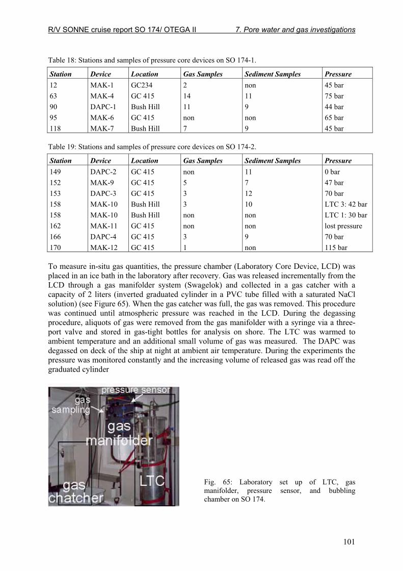
R/V SONNE cruise report SO 174/ OTEGA II 7. Pore water and gas investigations
101
Table 18: Stations and samples of pressure core devices on SO 174-1.
Station Device Location Gas Samples Sediment Samples Pressure 12 MAK-1 GC234 2 non 45 bar
63 MAK-4 GC 415 14 11 75 bar
90 DAPC-1 Bush Hill 11 9 44 bar
95 MAK-6 GC 415 non non 65 bar
118 MAK-7 Bush Hill 7 9 45 bar Table 19: Stations and samples of pressure core devices on SO 174-2.
Station Device Location Gas Samples Sediment Samples Pressure 149 DAPC-2 GC 415 non 11 0 bar
152 MAK-9 GC 415 5 7 47 bar
153 DAPC-3 GC 415 3 12 70 bar
158 MAK-10 Bush Hill 3 10 LTC 3: 42 bar
158 MAK-10 Bush Hill non non LTC 1: 30 bar
162 MAK-11 GC 415 non non lost pressure
166 DAPC-4 GC 415 3 9 70 bar
170 MAK-12 GC 415 1 non 115 bar To measure in-situ gas quantities, the pressure chamber (Laboratory Core Device, LCD) was placed in an ice bath in the laboratory after recovery. Gas was released incrementally from the LCD through a gas manifolder system (Swagelok) and collected in a gas catcher with a capacity of 2 liters (inverted graduated cylinder in a PVC tube filled with a saturated NaCl solution) (see Figure 65). When the gas catcher was full, the gas was removed. This procedure was continued until atmospheric pressure was reached in the LCD. During the degassing procedure, aliquots of gas were removed from the gas manifolder with a syringe via a three-port valve and stored in gas-tight bottles for analysis on shore. The LTC was warmed to ambient temperature and an additional small volume of gas was measured. The DAPC was degassed on deck of the ship at night at ambient air temperature. During the experiments the pressure was monitored constantly and the increasing volume of released gas was read off the graduated cylinder
Fig. 65: Laboratory set up of LTC, gas manifolder, pressure sensor, and bubbling chamber on SO 174.

R/V SONNE cruise report SO 174/ OTEGA II 7. Pore water and gas investigations
102
After degassing, the cores were recovered from the pressure chambers and sampled for pore water analysis, physical properties (see chapter 6) and remaining gases. The stored gas samples will be analyzed for C1-C5 hydrocarbons and their stable carbon isotopes. Bush Hill
The gas volume collected from the pressure cores taken at Bush Hill ranged between 50 and 64,000 ml of gas. Pressure cores which contained free gas and gas hydrates were characterized by a slower decrease in pressure during degassing and an increase in pressure at times when the valves were closed (Figure 66). The pressure variations accompanying the gas release reflect the discontinuous degassing of the core, which was observed in the gas catcher during the period of main gas release. The strongest decrease in pressure taking place at the beginning is accompanied by a release of water. The composition of a gas sample from the pressure core shown below (MUK 07) was very similar to that of decomposing gas hydrate from Bush Hill, containing C1 – C4 hydrocarbons.
0
5
10
15
20
25
30
35
0 50 100 150 200 250 300 350 400
0
200
400
600
800
1000
1200
1400
Time [min]
Pre
ssure
[bar]
Volu
me [m
l]
MAK 07 - Bush Hill
Volume [ml]
Pressure [bar]
Fig. 66: Pressure files and gas volume increase during the degassing of MAK 07 and DAPC 04.
Green Canyon (GC 415, GC 234)
The gas volume collected from the pressure cores taken at GC 415 ranged between 50 and 14,000 ml of gas. Changes of pressure and gas volume encountered during degassing are similar to those observed in the Bush Hill core, as are the C1 – C4 ratios from gas measurements carried out on board. All this might indicate a dissociation of structure II gas hydrate. Further indications were found in some of the sediment cores recovered from the pressure chambers after degassing. Very little gas was found in MAK-1 from GC 234, where no indications of gas hydrate were found in any of the measurements.

R/V SONNE cruise report SO 174/ OTEGA II 8. Microbial ecology
103
8. MICROBIAL ECOLOGY
8.1 Leg SO 174-1
Tina Treude, Matthew Erickson and Marion Kohn1 In former investigations (Joye et al. 2004) geochemical characteristics of sediments were detected and rates of anaerobic oxidation of methane (AOM) and sulfate reduction (SR) were measured in samples collected near thermogenic (structure II) gas hydrate mounds and in areas lacking hydrates along the continental slope in the Gulf of Mexico. Radiotracer (C-14 and S-35) techniques were used to determine rates of AOM and SR over depth in sediment cores. Abundant mats of white and orange Beggiatoa spp. were common in areas of active seepage and these sediments were enriched in hydrogen sulfide and methane. In cores collected from areas without Beggiatoa or hydrate, concentrations of redox metabolites showed little variation over depth and these sites were inferred to be areas of low seepage. Integrated AOM rates were low in Beggiatoa-free cores (<0.05 mmol m-2 d-1) and averaged 2.8±4.6 mmol m-2 d-1 in seep cores that contained Beggiatoa or gas hydrate. Integrated SR rates were also low in Beggiatoa-free cores (<1 mmol m-2 d-1) and averaged 54±94 mmol m-2 d-1 in cores with Beggiatoa or hydrate. Rates of SR generally exceeded rates of AOM and the two processes were loosely coupled, suggesting that the majority of SR at Gulf of Mexico hydrocarbon seep sites is likely to be fueled by the oxidation of other organic matter, possibly other hydrocarbons and oil, rather than by AOM. On OTEGA II, leg 1 we deepened the study on AOM and SR at sites covered by either white or orange Beggiatoa mats to investigate differences between them and to find correlations with the presence of methane or oil. We combined measurements on microbial turnover rates with molecular, microbiological, pore water and biomarker investigations to gain a full picture of the biogeochemical processes. Beside AOM/SR, the second emphasis of this cruise was the quantification of methanogenesis with 14C-labeled acetate and bicarbonate. Table 20: Sample data leg SO 174- 1.
Station No. Instrument Sampling1)
Surface Location
8-2 TV-MUC Core 1-4 White Beggiatoa Bush Hill 38-2 TV-MUC Core 1-4 White Beggiatoa Bush Hill 55 TV-MUC Core 1-4 White Beggiatoa Bush Hill 78 BIGO Core 1 Orange Beggiatoa GC234 87 TV-MUC Core 1-3 Orange Beggiatoa GC234 111 TV-MUC Core 1-3 Orange Beggiatoa GC234
1) For description of the core sampling see text. Sediment samples were taken from 5 TV-MUC and 1 BIGO deployment (Table 20). 3 white and 3 orange Beggiatoa mats altogether were sampled from Bush Hill and GC234, respectively. Cores were immediately transported to a cooling room (4°C) after recovery. 3 to 4 cores from one haul were sub-sampled as follows:
Core 1 (AOM and SR)
Subsampling in 2-cm intervals (max 30 cm) Parameters: AOM, SR, methane, sulfate, porosity, DNA, biomarkers

R/V SONNE cruise report SO 174/ OTEGA II 8. Microbial ecology
104
Core 2 (methanogenesis)
Subsampling in 2-cm intervals (max 30 cm) Parameters: methanogenesis (substrate acetate), methanogenesis (substrate bicarbonate), hydrogen, sulfide, dissolved inorganic carbon (DIC), volatile fatty acids (VFA), fluorescence in situ hybridization (FISH), bacterial counts Core 3 (microbiology)
Samples for in vitro experiments on AOM and methanogenesis Subsampling: 0-2 cm (oxic storage), 2-10 cm (anoxic storage), 10-20 cm (anoxic storage) Core 4 (microbiology)
Samples for in vitro experiments on acetogenesis Subsampling: 0-2 cm (oxic storage), 2-10 cm (anoxic storage), 10-20 cm (anoxic storage) BIGO sediment was sampled according to Core 1 (max 12 cm). Preliminary results
Due to the long processing time for microbiological samples, no results are available at this time.
8.2 Leg SO 174-2
Beth Orcutt and Imke Müller To our knowledge, no previous data has been reported on the sedimentary microbial biogeochemistry of the new Campeche and Sigsbee sites targeted during leg 2. It is reasonable to assume that active, hydrocarbon-based chemosynthetic communities could reside at these new sites based on oil slick surveys (I. R. MacDonald, personal communication). Previous work at Gulf of Mexico cold seeps indicates active hydrocarbon-based microbial ecosystems both within the sediments (Joye et al. 2004, see 5.1 for summary) and within hydrate material (Orcutt et al. 2004). The microbiology goals of the second leg of the OTEGA II project aimed to broaden the understanding of hydrocarbon cycling in the Gulf of Mexico basin. Similar to aims of the first leg, the microbiology group was mainly interested in documenting the distribution, magnitude, and interactions of AOM, SR and methanogenesis at these cold seep sites. We combined measurements on microbial turnover rates with molecular, microbiological, pore water and biomarker investigations to gain a full picture of the biogeochemical processes. A particular interest on this leg was the comparison of the microbial communities at the new Gulf of Mexico seep sites with previous work at the northern seep sites (Joye et al. 2004, Orcutt et al. 2004). On the second leg of the OTEGA II SONNE 174 research cruise, three main sampling goals were accomplished. The first goal encompassed collection of hydrocarbon-rich sediment and hydrate, as well as asphalt-containing material, from the new Campeche-area sites. Collection of gas hydrate and hydrate-bearing sediments from Bush Hill fulfilled the second goal. Finally, sampling at the new GC415 site in the northern Gulf of Mexico satisfied the final aim.

R/V SONNE cruise report SO 174/ OTEGA II 8. Microbial ecology
105
Table 20: Sample data leg SO 174-2.
Station Device Site Description
Multicore Profiling
133 MUC 16 Campeche typical marine sediment
139 MU 17 Chapopote typical marine, slightly sulfidic
140 TVG 6 Chapopote hydrate, very oily, disturbed
149 DAPC 2 GC415 oil, gassy, sulfidic
150 TGC 1 GC415 oil, gassy, hydrate
156 MUC 18 GC185 white mat, very gassy, sulfidic
166 DAPC4 GC415 carbonate, sulfidic
Grab samples
136 TVG 5 Chapopote asphalt and mud
140 TVG 6 Chapopote hydrate
140 TVG 6 Chapopote hydrate sediment
156 MUC 18 GC185 15+ cm sediment
157-2 TVG 10 GC185 hydrate sediment
157-2 TVG 10 GC185 hydrate
159 GC 12 GC185 30cm, carbonate
159 GC 12 GC185 85cm, hydrate
161 MUC 19 GC415 hydrate sediment
161 MUC 19 GC415 hydrate
161 MUC 19 GC415 carbonate, oil, 20+cm
161 MUC 19 GC415 carbonate, oil, 0-10cm
163 TVG 11 GC 415 hydrate, carbonate tubes
169 TVG 12 GC 415 hydrate, oily sediment
171 TGC 3 GC415 hydrate sediment, top 1m
171 TGC 3 GC415 dark gray sediment, lower 1m The microbiology sampling strategy on leg 2 differed slightly from leg 1. Increased emphasis was placed on collecting samples from deeper sedimentary layers than were available from TV-MUC or BIGO deployments. As such, samples were collected from DAPC, GC, and TGC cores in addition to TV-MUC and TV-Grab samples (Table 2). Additionally, microbiology samples were collected from grab samples of hydrate, oil, and asphalt material. This sampling strategy was adopted in an effort to develop a more comprehensive understanding of hydrocarbon cycling in these seep systems. After collection, samples were immediately transferred to a 4oC cold room for processing. Due to sample size limitation, the full suite of sub-sampling could not be performed on all samples collected. For brief description of samples, please see Table 20. More detailed descriptions of sample environment follow below.

R/V SONNE cruise report SO 174/ OTEGA II 8. Microbial ecology
106
Station 133, Campeche, MUC 16
Cores were collected next to a patch of brownish, leathery material in an area with abundant snail trails, some irregular carbonates and few shells. Cores processed by the Pore water group had pieces of this leathery material, but these conspicuous items were absent from the one core processed for microbiology. No visible mat. Sediment in top 5 cm was light brown, gradually changing to creamy gray, sticky ooze with depth. Slight sulfidic odor at the bottom of the core. Parameters measured: AOM, SR, FISH/BAC, DNA, sulfate, porosity, methane, hydrogen, biomarker Station 136, Chapopote, TVG 5
Sticky light gray nano-fossil ooze and fine brownish sediment covering massive asphalt chunks.
Parameters measured: FISH, biomarker, taken home for microbiological studies.
Station 139, Chapopote, MUC 17
In appearance, sediment similar to cores collected during MUC16, with the exception of no leathery/tar pieces. Cores collected adjacent to an area with small (<1cm relief) mounded white domes, possibly a white mat. Sediment surface in cores had a sparse collection of thin grayish/white filaments 2-3 mm in length and a few rounded, 1-2 mm in diameter, light gray microorganisms. As in MUC16, bottom of core had slight sulfidic odor. Parameters measured: AOM, SR, FISH/BAC, DNA, sulfate, porosity, methane, hydrogen, biomarker, take home samples for microbiological analysis. Station 140, Chapopote, TVG 6
MUC corers were pushed through part of TV-Grab sample containing oily, disturbed sediment with active hydrate dissocation. Cores contained porous carbonate chunks as well. Also collected: bottled samples of sediment-rich, oily hydrate; viscous oil with sediment; and more sediment with bubbling hydrate. Parameters measured: AOM, SR, Bi-MoG, Ace-MoG, FISH/BAC, DNA, sulfate, porosity, methane, hydrogen, VFAs, sulfide, DIC, biomarker, mud taken home for microbiological analysis. Station 149, GC415, DAPC 2 Dark olive, gassy sediment. Lower layers contained oil and carbonates and had strong sulfidic smell. Microbiology samples were collected from sediment immediately beneath samples for pore water group. Parameters measured: AOM, SR, FISH/BAC, DNA, biomarker, methane, sulfate, porosity. Station 150, GC415, TGC 1 Sediments disturbed from hydrate dissociation while core was on deck. Refined, yellowish oil in sediments in areas with hydrate. Gassy sediment, little carbonate found. Parameters measured: AOM, SR, FISH/BAC, DNA, biomarker, methane, sulfate, porosity.

R/V SONNE cruise report SO 174/ OTEGA II 8. Microbial ecology
107
Station 156, GC185, MUC 18 Sediment collected a few meters west of the famous mound at Bush Hill. After flying TV-MUC over the LSU Bubble-o-meter frame, cores set down in a white mat directly adjacent to a large tube worm bush. Cores were extremely gassy and sulfidic, some cores had bubbling hydrate at the base, but no carbonate. Parameters measured: AOM, SR, Bi-MoG, Ace-MoG, FISH/BAC, DNA, biomarker, methane, sulfate, porosity, hydrogen, VFAs, DIC, sulfide, sediment taken home for microbiological analysis; additional VFA samples collected for L. Hmelo. Station 157-2, GC185, TVG 10 Massive hydrate collection under a white mat with grayish/black areas. Sheets and chunks of white hydrate, with little yellowish oil veined in sediments. Collected bottles of hydrate-rich sediment and separate bottles of “clean” white hydrate. Parameters measured: AOM, SR, FISH/BAC, DNA, biomarker, methane, sulfate, porosity, take home mud for microbiological analysis. Station 159, GC185, GC 12
Hydrate-rich grayish sediment with yellow oil, disturbed from hydrate disassociation. Collected one sample from 85cm depth which had a large hydrate chunk, bubbles, sediment. Another sample from a depth of 30 cm which had less hydrate but did have carbonate chunks. Parameters measured: AOM, SR, FISH/BAC, DNA, biomarker, methane, sulfate, porosity, take home mud for microbiological analysis. Station 161, GC415, MUC 19 TV-MUC set down in a large white mat patch with grayish and black areas; this white patch was adjacent to an area with carbonate outcrops and shells. Immediately after core penetration, massive release of gas and oil was evidenced on video (approximately 15:32:00 on video); release continued for several minutes. Upon retrieval, active hydrate dissociation was observed in cores. Sediment was very oily and hydrate- rich, also containing carbonate nodules. Microbiology cores were too disturbed for profiled processing, so sediment material was collected into bottles for further processing. Parameters measured: AOM, SR, Bi-MoG, Ace-MoG, FISH/BAC, DNA, biomarker, methane, sulfate, porosity, hydrogen, VFAs, DIC, sulfide, sediment takn home for microbiological analysis.
Station 163, GC415, TVG 11 Disseminated hydrate, massive carbonate tubes, not as oily as other grabs. Collected one bottle of sediment to take home for microbiological analysis.
Station 166, GC415, DAPC 4 Dark olive-gray sediments with carbonates and oil. Microbiology samples were collected from sediment immediately beneath samples for pore water group. Parameters measured: AOM, SR, FISH/BAC, DNA, biomarker, methane, sulfate, porosity. Station 169, GC415, TVG 12 After passing through flare, TV-Grab set down on a scattered patch of white and gray mat next to carbonate. Sediment contained abundant disseminated hydrate, oil and massive

R/V SONNE cruise report SO 174/ OTEGA II 8. Microbial ecology
108
carbonates. Collected one bottle of bubbly, oily sediment for take home microbiological analysis. Station 171, GC415, TGC 3 Upper meter of core was disturbed from hydrate dissociation. Lower meter of the core was more compact, drier dark gray sediment with little oil or hydrate evident. One pooled sample was bottled from the upper meter with hydrate, another pooled sample was bottled from the lower sediment. Samples collected to take home sediment for microbiological analysis. Preliminary results
Due to the long processing time for microbiological samples, no results are available at this time.

R/V SONNE cruise report SO 174/ OTEGA II 9. Biological sampling
109
9. BIOLOGICAL SAMPLING
Elva Escobar-Briones Sediment samples were collected in the northern, central and southwestern Gulf of Mexico abyssal plain during the OTEGA II cruise in the month of October. The biological samples collected were of seven types: � meiofauna samples collected along different depths in the cores collected with the
multiple corer � foraminifera samples collected along different depths in the cores collected with the
multiple corer � bacteria samples collected along different depths in the cores collected with the multiple
corer � foraminifera samples collected from different depths from the gravity corer � bacteria samples collected from different depths from the gravity corer � megafaunal scavengers collected with baited traps � megafauna collected in the TV grab At each sampling station where biological samples were obtained additional sediment replicates were sampled using 50-ml hand cores of 2.89 cm in diameter with a penetration depth into the the sediment of 5 cm. They were collected to perform analyses of sediment factors that included: � grain size � chloropigment concentration in superficial sediment � elemental organic carbon and nitrogen content in sediment � �13C and �15N stable isotope composition of the sediment organic matter in sediment The replicates sampled for chloropigments, elemental carbon,nitrogen and stable isotopes were frozen to –20°C onboard and will be analyzed in the laboratory in the next months. 9.1 Samples collected
Meiofauna
The three 0.0007 m2 meiofaunal replicates were sieved onboard through a 42 �m mesh after having been exposed to a freshwater shock. Each replicate was stored in 75-ml jars after sieving, fixed with 95% ethanol and Rose Bengal vital stain to make sorting in the laboratory easier and labeled. Foraminifera The 1cm3 foraminifera replicates were fixed onboard with 10% formaldehyde solution, buffer and Rose Bengal vital stain, stored in 50- ml centrifuge tubes and will be sorted, identified and quantified in the laboratory. Bacteria Three to five sediment replicates of 1 cm3 in volume were collected and frozen in liquid nitrogen onboard to sequence living heterotrophic bacteria in the laboratory.

R/V SONNE cruise report SO 174/ OTEGA II 9. Biological sampling
110
Megafauna Bivalve and tubeworm specimens obtained from TV grab samples were frozen at –20°C if captured alive and photographed later for an inventory of the megafauna captured in the southwestern abyssal stations. Other specimens were captured with the help of baited traps deployed on a lander for 36 hours. Their arrival and capture was recorded with a time lapse camera and they were photographed and fixed onboard for later systematic study in the formal national collections. 9.2 Laboratory activities
Meiofauna Each replicate will be hand-sorted first using a stereoscopic microscope with 5-fold magnification. This method will include placing subsamples of sediment in Petri dishes, extracting the specimens with fine-tip forceps, quantifying simultaneously to identifying to major taxa. Identification of the sorted specimens and quantification will allow to provide density and biomass data by placing the specimens in a loop slide (4x3) with a glycerine drop to take pictures with a Kodak DC290 digital camera using a zoom mounted to a stereoscopic Zeiss microscope with an 10/8 objective, these images will be used to calculate the biomass based on a biovolume strategy following the protocols described in Feller and Warwick (1979) and Warwick and Price (1979). The biovolume will be determined using the Sigma Scan Pro 5 software using a calibration image generating an Excel file. The calibration will be aided by a 2.00-mm micrometer. All measurements will be reported in micrometers. The “two dot calibration” option will be used to transform pixels to micrometers. A total of three measurements will be used to identify and determine the volume first and finally the biomass of each organism. Conversion factors will be used to transform the fixed wet weight biomass values to mg C.m-2 values in all dominant components. Grain size The grain size analysis will be made with a Fritsch Particle Sizer Analysette 20 Sedimentograph that uses the photo-extinction method measuring the degree of attenuation of a monochromatic light beam caused by the suspended particles along a period of time in a settling column. Sediment samples of 1gr in size will be sonicated in distilled water for 5 minutes to homogenize the materials and placed in a settling column filled with distilled water. A ”distilled water” blank will be used between replicates of each sample. The sediment will be suspended to obtain saturation levels of 55% to 70% and one-minute readings will be made on the sediment - distilled water homogenate. Every record will determine to each ½ � size between 4 to 12 �, and will be reported as percentage of occurrence. Elemental organic carbon and nitrogen The frozen sediment will be thawed at environmental temperature in the laboratory. The sediment will previously be acidified with a 0.1 N HCl solution to eliminate the excess carbonates. The sediment will rinsed with bi-distilled water to eliminate the excess acid solution. Each sediment sample will be left to evaporate at ambient temperature, those still containing water will be dried in a drying oven at 60°C. The sediment will be homogenized before being analyzed. The sediment will be placed in quartz vials and labeled, the percentage of elemental organic carbon and nitrogen will be determined in triplicate in a FISSONS

R/V SONNE cruise report SO 174/ OTEGA II 9. Biological sampling
111
elemental analyzer model EA1108 following the protocol suggested by Pella (1990). This method is based on a complete and instantaneous oxidation of the sample using “fast combustion” that transforms all the organic and inorganic material in combustion products. The resulting gas flows through a reduction oven transported by He carry gas into a chromatographic column where the gas is detected and sorted by a conductivity thermal detector (CTD) that responds proportionally to the individual contents in the mixture. Chloropigments in the sediment The frozen sediment samples collected for this analysis will be thawn in the laboratory at ambient temperature. The chloropigment extraction will carried out in darkness adding a total of 10 ml acetone 90% solution at 4°C for a 24-h period. After extraction the sediment-acetone solution will be centrifuged at 1,700 rpm for 15 minutes and eight ml will be drawn with a pipette and placed in 10x10mm glass cuvettes to make fluorescence readings at 680 nm in a 10-AU Turner Designs bench fluorometer, the values obtained will be expressed as μg Chla.cm-2 sediment. A 90% acetone blank will be used to extract to the fluorometer reading and multiplied by the dilution factor when made. The resulting value will be multiplied by the final volume of the acetone extract.

R/V SONNE cruise report SO 174/ OTEGA II References
112
REFERENCES
Aguirre Gomez R (2002) Primary production in the southern Gulf of Mexico estimated from solar-stimulated natural flourescence. Hidrobiologica 12, 1, 21-28
Aharon P, Fu BS (2000) Microbial sulfate reduction rates and sulfur and oxygen isotope fractionations at oil and gas seeps in deepwater Gulf of Mexico. Geochimica Et Cosmochimica Acta 64, 2, 233-246
Antoine JW (1972) Structure of the Gulf of Mexico In: Rezak R, Henry VI (Eds) Contributions on the Geological and Geophysical Oceanography of the Gulf of Mexico Gulf Publishing Co Houston pp1-34
Antoine JW, Bryant WR (1969) Distribution of salt and salt structures in Gulf of Mexico. American Association of Petrology and Geology Bulletin 53, 12, 2543-2550
Antoine JW, Martin RG, Pyle TG, Bryant WR (1974) Continental margins of the Gulf of Mexico. In: Burk CA, Drake CL (eds): The geology of continental margins. Springer-Verlag New York, 683-693
Behrens EW (1988) Geology of a continental slope oil seep, northern Gulf of Mexico. American Association of Petroleum Geologists Bulletin 72, 2, 105-114
Bergantino RN (1971) Submarine regional geomorphology of the Gulf of Mexico. Geological Society American Bulletin 82, 741-752
Boetius A, Lochte K (2000) Regional variation of total microbial biomass in sediments of the deep Arabian Sea. Deep-Sea Research II, 47, 149-168
Boetius A, Suess E. (in press) Hydrate Ridge: a natural laboratory for the study of microbial life fueled by methane from near-surface gas hydrates. Chemical Geology
Bohrmann G, Schenck S (2002) Cruise Report M 52-1 MARGASCH. Report No. 108, GEOMAR, Kiel
Bouma HA (1972) Distribution of sediments and sedimentary structures in the Gulf of Mexico. In: Rezak R, Henry V J (eds): Contribution on the Geological and Geophysical Oceanography of the Gulf of Mexico. Texas A & M University, Oceanography studies, Gulf Pub, Houston, Texas, 3, 35-65
Bryant WR, Lugo J, Córdova C, Salvador A (1991) Physiography and Bathymetry. In: Salvador A (ed): The Gulf of Mexico Basin, V, J Geol Soc Am, Boulder, Colorado, 13-30
Carney RS (1994) Consideration of the oasis analogy for chemosynthetic communities at Gulf of Mexico hydrocarbon vents. Geo-Marine Letters 14, 2/3, 149-159
Cook D, D'Onfro P (1991) Jolliet Field thrust fault structure and stratigraphy, Green Canyon Block 184, offshore Louisiana. Transactions-Gulf Coast Association of Geological Societies XLI, 100-121
Czerna Z (1984) Margen continental de colisión en la parte sur occidental del Golfo de México. Rev Inst Geol 5, 255-261
Davies DK (1968) Carbonate turbidites, Gulf of Mexico. J Sedimentary Petrology 38, 1100-1109
De Beukelaer S, MacDonald I R, et al (2003) Distinct Side-Scan Sonar, RADARSAT, SAR, and Chirp Signatures of Gas and Oil Seeps on the Gulf of Mexico Slope. Geo-Marine Letters October

R/V SONNE cruise report SO 174/ OTEGA II References
113
Dickens GR (2003) Rethinking the global carbon cycle with a large, dynamic and microbially mediated gas hydrate capacitor. Earth and Planetary Science Letters 213, 169-183
Elliot BA (1982) Anticyclonic rings in the Gulf of Mexico. J Phys Oceanogr 12, 1292-1309
Ewig M, Antoine JW (1966) New seismic data concerning sediments and diapiric structures in Sigsbee Deep and continental slope, Gulf of Mexico. American Association of Petrology and Geology Bulletin 50, 3, 479-504
Feely, Kulp (1957) AAPG bull 41, 1802
Feller RJ, Warwick RM (1979) Energetics. In: Higgins RP, Thiel H (eds) Introduction to the study of meiofauna. Smitsonian, Washington p181-196.
Fisher CR, MacDonald IR, et al (2000) Methane ice worms: Hesiocaeca methanicola colonizing fossil fuel reserves. Naturwissenschaften 87, 4, 184-187
Gallegos A, Czitrom S, Zavala J, Fernández A (1993) Scenario modeling of climate change on the ocean circulation of the Intra –Americas Sea. In: Maul GA (ed): Climatic change in the Intra-Americas Sea, UNEP 55 – 74
Garrison LE, Martin RG (1973) Geologic structures in the Gulf of Mexico Basin. US Geol Survey Prof paper 773, 85 p
Grasshoff M, Ehrhardt K, Kremling K (1983) Methods of seawater analysis, Vol. Verlag Chemie, Weinheim
Hamilton P (1990) Deep currents in the Gulf of Mexico. J Phys Oceanogr 20, 85-90
Hoffman EE, Worley SJ (1986) Circulation of the Gulf of Mexico. Journal of Geophysical Research 91, 14221-14236
Ivanenkov VN, Lyakhin YI (1978) Determination of total alkalinity in seawater. In: Bordovsky OK, Ivanenkov VN (eds) Methods of hydrochemical investigations in the ocean. Nauka Publ. House, Moscow, p 110-114
Joye SB, Boetius A, Orcutt BN, Montoya JP, Schulz HN, Erickson MJ, Lugo SK (2004) The anaerobic oxidation of methane and sulfate reduction in sediments from Gulf of Mexico cold seeps. Chemical Geology 205, 219-238
Kirkland, Gerhard (1971) AAPG bull 55 p 680
Kvenvolden KA, Lorenson TD (2001) The global occurrence of natural gas hydrates. In: Paull C (ed) Natural gas hydrates: Occurrence, distribution, and detection. American Geophysical Union, p 3-18
Kvenvolden, KA (1995) A review of the geochemistry of methane in natural gas hydrate. Organic Geochemistry 23 (11-12), 997-1008.
Lammers S, Suess E (1994) An improved head-space analysis method for methane in seawater. Marine Chemistry 47, 115-125.
Larkin J, Aharon P, Henk MC (1994) Beggiatoa in microbial mats at hydrocarbon vents in the Gulf of Mexico and warm mineral springs, Florida. Geo-Marine Letters 14, 97-103
MacDonald IR, Boland GS, et al (1989) Gulf of Mexico chemosynthetic communities II: spatial distribution of seep organisms and hydrocarbons at Bush Hill. Marine Biology 101, 235-247
MacDonald IR, Guinasso Jr NL, et al (1993) Natural oil slicks in the Gulf of Mexico visible from space. Journal of Geophysical Research 98, C9, 16351-16364

R/V SONNE cruise report SO 174/ OTEGA II References
114
MacDonald IR, Guinasso Jr NL, et al (1994) Gas hydrate that breaches the sea floor on the continental slope of the Gulf of Mexico. Geology 22, 699-702
MacDonald IR, Sager WW, et al (2003) Association of Gas Hydrate and Chemosynthetic Fauna in Mounded Bathymetry at Mid-Slope Hydrocarbon Seeps: Northern Gulf of Mexico. Marine Geology 198, 133-158
Macgregor D (1993) Relationships between seepage, tectonics and subsurface petroleum reserves. Marine and Petroleum Geology 10, 606-619
Max M (2000) Natural gas hydrate in oceanic and permafrost environments. Kluwer Academic Publishers, 414 pp
McGookey DP (1975) Gulf Coast Cenozoic sediments and structures: an excellent example of extra-continental sedimentation: Gulf Coast Association of Geological Societies Transactions 25, 104 – 120.
Moore GW, Del Castillo L (1974) Tectonic evolution of the southern Gulf of Mexico. Geological Society Annual Bulletin 85, 4, 607-618
Morrison JM, Nowlin WD (1977) Repetead nutrient, oxygen, and density section through the Loop Current. J Mar Res 35, 105-128
Müller Kärger FE, Walsh JJ (1991) On the seasonal phytoplankton concentration and sea surface temperature cycles of the Gulf of Mexico as determined by satellites. J of Geophys Res, 96, 12645 – 12665
Nelson (1991) Salt tectonics and listric-normal faulting. In: Salvador A (ed), The Gulf of Mexico Basin, The geology of North America, V, J Geol Soc Am, Boulder, Colorado
Norris, RD, Röhl U (1999) Carbon cycling and chronology of climate warming during the Palaeocene/Eocene transition. Nature 401, 775-778.
Nowlin WD (1971) Water Masses and general circulation of the Gulf of Mexico. Ocean Cont 452, 173 –178
Nowlin WD, McLellan HJ (1967) A characterization of Gulf of Mexico waters in winter. Journal of Marine Research 25, 1, 29-59
Olu K, Lance S, Sibuet M, Henry P, Fiala-Médioni A, Dinet A (1997) Cold seep communities as indicators of fluid expulsion patterns through mud volcanoes seaward of the Barbados accretionary prism. Deep-Sea Res 44, 811-841
Orcutt BN, Boetius A, Lugo SK, MacDonald IR, Samarkin VA, Joye SB (2004) Life at the edge of methane ise: microbial cycling of carbon and sulfur in Gulf of Mexico gas hydrates. Chemical Geology 205, 239-251
Paull C (ed) (2001) Natural gas hydrates: Occurrence, distribution, and detection, Vol 124. American Geophysical Union
Pella, E (1990) Elemental organic analysis. Part 1, Historical developments. American Laboratory 22(2),116–25.
Pequegnat WE (1972) A deep bottom current on the Mississippi Cone. In: Capurro LRA, Reid JL (eds): Contributions to the Physical Oceanography of the Gulf of Mexico. Texas A&M Univ Oceanogr Stud 2, 65-87
Pequegnat WE (1983) The ecological communities of the continental slope and adjacent regimes of the northern Gulf of Mexico. Prepared by TerEco Corporation for Minerals Management Service, US Department of the Interior, Contract AA851-CT1-12 398 p + Append

R/V SONNE cruise report SO 174/ OTEGA II References
115
Pfannkuche O, Eisenhauer A, Linke P, Utecht C (2002) RV Sonne Cruise Report SO 165 OTEGA I, Balboa – San Diego – Portland – San Francisco, June 29 – August 29 2002. GEOMAR
Pfannkuche O, Linke O (2003) GEOMAR landers as long-term deep sea observatories. Sea Technology 44, 9, 50-55
Pindell, JL (1985) Alleghenian reconstruction and the subsequent evolution of the Gulf of Mexico, Bahamas and proto-Caribbean. Tectonics 4 (1), 1-39.
Reilly JF, MacDonald IR, et al (1996) Geologic controls on the distribution of chemosynthetic communities in the Gulf of Mexico. Hydrocarbon migration and its near-surface expression. Schumacher D, Abrams MA, Tulsa, OK, Amer Assoc Petrol Geol 38-61
Rezak R, Edwards GS (1972) Carbonate sediments of the Gulf of Mexico. In: Rezak R, Henry VJ (eds): Contributions on the Geological and Geophysical Oceanography of the Gulf of Mexico, Texas A & M University Oceanographic Studies 3, 263-280
Ricci-Lucci F, Valmori E (1980) basin-wide turbidites in a miocene, oversupplied deep-sea plain: a geometrical analysis. Sedimentology 27, 241-270
Roberts HH, Aharon P (1994) Hydrocarbon-derived carbonate buildups of the northern Gulf of Mexico continental slope: A review of submersible investigations. Geo-Marine Letters 14, 135-148
Roberts HH, Carney RS (1997) Evidence of episodic fluid, gas, and sediment venting on the northern Gulf of Mexico continental slope. Economic Geology and the Bulletin of the Society of Economic Geologists 92, 7-8, 863-879
Rothwell RG, Reeder MS, Anastasakis G, Stow DAV, Thomson J, Kahler G (2000) Low sea-level stand emplacement of megaturbidites in the western and eastern Mediterranean Sea. Sedimentary Geology 135, 75-88
Rupke NA (1975) Deposition of fine-grained sediments in the abyssal environments of the Algero-Baleric basin, western Mediterranean Sea. Sedimentology 22, 95-109
Sahling H, Rickert D, Linke P, Suess E, Lee RW (2002) Community structure at gas hydrate deposits at the Cascadia convergent margin, NE Pacific Mar Ecol Prog Ser 231, 121-138
Salas de Leon DA, Monreal Gomez MA (1997) Circulación y estructura termohalina del Golfo de México. Contribuciones a la Ocenografía Física en México Unión, Geofísica Mexicana Monografía No 3
Sassen R, Losh SL, III LC, Roberts HH, Whelan JK, Milkov AV, Sweet ST, DeFreitas DA (2001) Massive vein-filling gas hydrate: relation to ongoing gas migration from deep subsurface in the Gulf of Mexico. Marine and Petroleum Geology 18, 551-560
Sassen R, Mac Donald IR, Requejo AG, Guinasso Jr NL, Kennicutt II MC, Sweet ST, Brooks JM (1994) Organic geochemistry of sediments from chemosynthetic communities, Gulf of Mexico slope. Geo-Marine Letters 14, 110-119
Sassen T, Sweet ST, et al (1999) Geology and geochemistry of gas hydrates, central Gulf of Mexico continental slope. College Station, Geochemical and Environmental Research Group, Texas A&M University
Shanmugam G, Moiola RJ (1984) Eustatic control of calciclastic turbidites. Marine Geology 56, 273-278.
Skoan E.D (1998) Clathrate hydrates of natural gases. Marcel Dekker, New York

R/V SONNE cruise report SO 174/ OTEGA II References
116
Sloan EDj (1998) Physical/chemical properties of gas hydrates and application to world margin stability and climatic change. In: Henriet JP, Mienert J (eds) Gas Hydrates: Relevance to World Margin Stability and Climate Change, Vol 137. Geological Society, London, p 31-50
Sommer S, Pfannkuche O, Rickert D, Kähler A (2002) Ecological implications of surficial marine gas hydrates for the associated small-sized benthic biota at the Hydrate Ridge (Cascadia Convergent Margin, NE Pacific). Mar Ecol Prog Ser 243, 25-38
Sturges W, Evans JC, Welsh S, Holland W (1993) Separation of warm-core rings in the Gulf of Mexico. Journal of Geophysical Oceanography 23, 250 – 268
Suess E, Torres ME, Bohrmann G, Collier RW, Greinert J, Linke P, Rehder G, Trehu A, Wallmann K, Winckler G, Zuleger E (1999) Gas hydrate destabilization: Enhanced dewatering, benthic material turnover and large methane plumes at the Cascadia convergent margin. Earth Planet Sci Lett 170, 1-15
Tomczak M, Godfrey JS (1994) Regional Oceanography: an Introduction. Pergamon, Oxford, 442 pp.
Uchupi E (1975) Physiography of the Gulf of Mexico and Caribbean Sea. In: Nairn AEM (ed): The ocean basins and margins, Vol 3, The Gulf of Mexico and the Caribbean, Plenum Press 1 – 64
Vidal FV, Vidal VM, Rodríguez PF, Zambrano L, Casillas J, Rendón R, Jaimes de la Cruz B (1998) Circulación del Golfo de México. Revista de la Sociedad Mexicana de Historia Natural 46, 1 – 15
Vidal VM, Vidal FV, Hernández AF (1990) Atlas oceanográfico del Golfo de México 2, Instituto de Investigaciones Eléctricas, Cuernavaca, Morelos, México, 707 p
Vidal VM, Vidal FV, Pérez-Molero JM (1992) Collision of a loop current anticyclonic ring against the continental shelf slope of the Western Gulf of Mexico. Journal of Geophysical Research 97, 2155 – 2172
Warwick RM, Price R (1979) Ecological and metabolic studies on free-living nematodes from an estuarine mud-flat. Estuarine Coastal Mar Sci 9, 257–271
Weiss RF (1970) The solubility of nitrogen, oxygen and argon in water and seawater. Deep-Sea Research 17, 721-735
Welsh SE, Inoue M (2000) Loop current rings and the deep circulation in the Gulf of Mexico. Journal of Geophysical Research C Oceans 105, C7, 16951 – 16959
Worzel JL, Bryant W et al (1973) Initial reports of the deep-sea drilling project, V X Washington, US Gov Printing office, 716
Yaorong Qian A, Jochens E, Kennicutt II MC, Biggs D (2003) Spatial and temporal variability of phytoplankton biomass and community structure over the continental margin of the northeast Gulf of México based on pigment analysis. Contshelf res 23, 1 –17

R/V SONNE cruise report SO 174/ OTEGA II Appendix
117
APPENDIX
Appendix 1: List of stations
Appendix 2: Lithologies sampled by lander deployments
Appendix 3: Lithologies sampled by multicorer
Appendix 4: MacDonald IR et al. (2004) Asphald Volcanism and Chemosynthetic
Life in the Campeche Knolls, Gulf of Mexico. Science 304, 999-1002

OTEGA II: R/V SONNE Cruise 174-1
Date 2003 Station Instrument Area Begin at seafloor off End Duration Latitude N° Longitude E° SSBL Water depth Recovery Remarks
(UTC) No. (UTC) max. depth seafloor (UTC) hh:mm begin: at sf. / end: off sf. begin: at sf. / end: off sf. (m)
Lousiana Slope8-Oct 1 CTD-1 0:30 1:19 2:20 1:50 26:49.78 90:19.09 2422 19 bottles sound velocity profile
8-Oct 2 CTD-2 Bush Hill 10:19 10:40 11:00 0:41 27:46.913 91:30.528 556 24 bottles water for BIGO
8-Oct 3 OFOS-1 Bush Hill 11:23 11:39 15:30 15:45 4:22 27:47.00 / 27:46.99 91:30.37 / 91:30.55 586
8-Oct 4 BWS-1 Bush Hill 16:40 17:22 17:37 18:01 1:21 27:46.943 91:30.514 X 548
8-Oct 5 PS-1 18:06 20:42 2:36 27:46.93 / 27:46.96 91:30.42 / 91:30.53 569 NBS profile, Flare Imaging - 1
8-Oct 6 DOS-1 Bush Hill 20:50 21:21 22:40 1:50 27:46.930 91:30.521 X 549
8-Oct 7-1 TV-MUC-1 Bush Hill 22:40 22:57 23:18 0:38 27:46.959 91:30.772 X 601 sediment disturbed
8-Oct 7-2 TV-MUC-2 Bush Hill 23:35 23:54 0:12 0:37 27:46.968 91:30.761 X 602 5 cores reference site
9-Oct 8-1 TV-MUC-3 Bush Hill 0:28 1:07 1:30 1:02 27:46.911 91:30.644 X 549 5 cores low penetration -> disposed
9-Oct 8-2 TV-MUC-4 Bush Hill 0:52 2:18 2:38 1:46 27:46.220 91:30.476 X 552 6 cores white Beggiatoa, Thiotrix, oil mud
9-Oct 9 PS-2 2:56 8:52 5:56 27:47.00 / 27:44.90 91:31.30 / 91:13.70 562
9-Oct 10 OFOS-2 GC 234 9:05 9:20 14:45 15:01 5:56 27:44.880 / 27:44.708 91:13.700 / 91:12.925 X 562
9-Oct 11 PS-3 15:50 18:39 2:49 27:44.285 / 27:44.820 91:13.432 / 91:13.500 615
9-Oct 12 MAC-1 GC 234 18:46 19:36 20:00 1:14 27:44.752 91:13.314 X 558 LTC 4: 45 bar, LTC 2: 0 bar
9-Oct 13 PS-4 20:05 22:12 2:07 27:44.77 / 27:47.03 91:13.38 / 91:30.60 590 NBS profile, Flare Imaging - 2
9-Oct 14 BIGO-1 Bush Hill 23:25 0:08 0:30 1:05 27:46.937 91:30.526 X 547 BIGO on bacterial mat
10-Oct 15 PS-5 0:50 9:03 8:13 27:44.43 / 27:43,29 91:29.41 / 91:16.99 844
10-Oct 16 OFOS-3 GC 233 9:08 9:22 12:32 12:50 3:42 27:43.237 / 27:43.085 91:16.862 / 91:16.570 670 aim: locating NR1 brine pool
10-Oct 17 PS-6 12:55 14:17 1:22 27:43.101 / 27:46,970 91:16.577 / 91:30.620 663
10-Oct 18-1 TV-MUC-5 Bush Hill 14:20 15:05 15:20 1:00 27:46.950 91:30.507 X 548 no release
10-Oct 18-2 TV-MUC-6 Bush Hill 15:30 16:22 16:40 1:10 27:46.951 91:30.536 X 550 6 coresbacterial mat for biogeo- and geochem.
exam10-Oct 19-1 TV-MUC-7 Bush Hill 17:00 17:22 17:30 0:30 27:46.926 91:30.472 X 553 no release
10-Oct 19-2 TV-MUC-8 Bush Hill 17:48 18:09 18:18 0:30 27:46.937 91:30.464 X 547 no release
10-Oct 20 CTD-3 Bush Hill 13:39 13:57 14:21 0:42 27:46.931 91:30.580 589 24 bottles water for BIGO + meth. profile
10-Oct 21 FLUFO-1 Bush Hill 21:00 21:36 21:52 0:52 27:46.924 91:30.483 X 562 deployment
10-Oct 22 BIGO-1 Bush Hill 21:50 21:56 22:27 0:37 27:46.94 91:30.60 588 recovery
10-Oct 23 TV-G-1 Bush Hill 23:41 0:37 0:55 1:14 27:46.944 91:30.506 X 584 half full recov. of mud, carbonate, tube worms
11-Oct 24 PS-7 1:17 9:50 8:33 27:46.86 / 27:33.82 91:30.75 / 90:58.04 603
11-Oct 25 OFOS-4 GC 415 9:55 10:21 14:45 15:08 5:13 27:33.894 / 27:33.508 90:58.082 / 90:59.0997 X 923
11-Oct 26 PS-8 15:13 18:25 3:12 27:33.60 / 27:46.87 90:59.12 / 91:30.45 864
11-Oct 27 GQ-1 Bush Hill 19:15 19:37 19:56 0:41 27:46.948 91:30.478 X 550 deployment
11-Oct 28 PS-9 20:05 23:25 3:20 27:47.15 / 27:46.92 91:31.45 / 91:30.62 600
12-Oct 29 BIGO-2 Bush Hill 0:13 0:37 0:52 0:39 27:46.932 91:30.544 X 554 BIGO on bacterial mat
12-Oct 30 CTD-4 Bush Hill 1:01 1:20 1:54 0:53 27:46.96 91:30.49 553 17 bottles CH4 water column profile
12-Oct 31 PS-10 2:03 9:38 7:35 27:46.98 / 27:25.19 91:31.30 / 91:22.43 1221
12-Oct 32 OFOS-5 GC 539 9:42 10:03 12:30 12:56 3:14 27:25.200 / 27:25.220 91:22.440 / 91:22.080 1238
12-Oct 33 PS-11 13:02 15:18 2:16 27:24.89 / 27:46.99 91:22.56 / 91:30.52 1241
12-Oct 34 DOS-1 Bush Hill 15:30 15:41 16:08 0:38 27:46.85 91:30.72 543 recovery
12-Oct 35 CTD-5 Bush Hill 16:16 16:33 16:53 0:37 27:47.009 91:30.715 603
12-Oct 36 PS-12 17:20 20:50 3:30 27:48.19 / 27:46.59 91:34.371 / 91:30.74 600
12-Oct 37 FLUFO Bush Hill 20:50 20:53 21:15 0:25 27:46.61 91:30.76 580 recovery
12-Oct 38-1 TV-MUC-9 Bush Hill 22:00 22:34 22:45 0:45 27:46.900 91:30.510 549 no release
12-Oct 38-2 TV-MUC-10 Bush Hill 23:16 23:40 23:55 0:39 27:46.927 91:30.478 X 547 6 cores white Beggiatoa on Bush Hill
13-Oct 39 BWS-2 Bush Hill 1:30 2:22 3:06 1:36 27:46.921 91:30.456 X 550

Date 2003 Station Instrument Area Begin at seafloor off End Duration Latitude N° Longitude E° SSBL Water depth Recovery Remarks
(UTC) No. (UTC) max. depth seafloor (UTC) hh:mm begin: at sf. / end: off sf. begin: at sf. / end: off sf. (m)
Lousiana Slope13-Oct 40 PS-13 3:10 7:05 3:55 27:47.37 / 27:32.07 91:30.35 / 90:59.35 1088
13-Oct 41 PS-14 GC 415 7:10 11:45 4:35 27:32.20 / 27:30.70 90:59.50 / 90:01.90 1093 Flare Imaging - 3
13-Oct 42 PS-15 11:45 14:23 2:38 27:30.70 / 27:46.81 90:01.90 / 91:30.39 950
13-Oct 43 BWS-3 Bush Hill 14:48 15:05 15:16 15:35 0:47 27:46.939 91:40.414 X 554
13-Oct 44 DOS-2 Bush Hill 17:55 18:29 18:50 0:55 27:46.930 91:30.495 X 547 deployment
13-Oct 45 BIGO-2 Bush Hill 19:04 19:06 19:35 0:31 27:.46.90 91:30.76 550 recovery
13-Oct 46-1 MAC-2 Bush Hill 20:22 21:09 21:30 1:08 27:46.949 91:30.453 X 547 no release
13-Oct 46-2 MAC-3 Bush Hill 21:30 21:54 22:15 0:45 27:46.925 91:30.491 X 545 one LTC under pressure
13-Oct 47-1 GC-1 Bush Hill 22:50 23:04 23:13 0:23 27:46.950 91:30.440 548 GH, no recovery, tubing damaged
13-Oct 47-2 GC-2 Bush Hill 23:41 23:53 23:59 0:18 27:46.949 91:30.440 547 2.8m GH from 2 m
14-Oct 48 FLUFO-2 Bush Hill 2:00 2:33 2:55 0:55 27:46.942 91:30.527 X 546 deployment
14-Oct 49 PS-16 3:00 6:20 3:20 27:46.97 / 27:24.08 91:30.73 / 91:21.31 1200
14-Oct 50 PS-17 GC 539 6:25 12:10 5:45 27:24.67 / 27:26.90 91:21.26 / 91:21.30 1200
14-Oct 51 PS-18 12:26 14:56 2:30 27:26.13 / 27:46.98 91:21.40 / 91:30.38 1114
14-Oct 52 GQ-1 Bush Hill 15:02 15:04 15:25 0:23 27:46.91 91:30.53 550 recovery
14-Oct 53 PS-19 15:33 17:13 1:40 27:47.96 / 27:44.77 91:29.93 / 91:13.26 547
14-Oct 54 CTD-6 GC 234 17:07 17:27 17:58 0:51 27:44.772 91:13.279 X 549 18 bottles CH4 water column profile
14-Oct 55 TV-MUC-11 GC 234 18:17 18:53 19:15 0:58 27:44.714 91:13.269 X 569 5 cores orange Beggiatoa
14-Oct 56 TV-G-2 GC 234 19:48 21:20 21:32 1:44 27:44.770 91:13.310 549 full
14-Oct 57 PS-20 21:54 23:46 1:52 27:46.88 / 27:47.20 91:12.66 / 91.30.53 570
15-Oct 58 BIGO-3 Bush Hill 0:30 1:35 1:55 1:25 27:46.959 91:30.531 X 570 BIGO on bacterial mat
15-Oct 59 HDSD-1 Bush Hill 2:15 2:47 3:06 0:51 27:46.942 91:30.499 X 551 deployment
15-Oct 60 PS-21 3:15 13:55 10:40 27:46.72 / 27:31.85 91:29.83 / 90:59.74 1050
15-Oct 61 PS-22 GC 415 13:55 15:25 1:30 27:31.89 / 27:32.69 90:59.74 / 90:59.87 1050 Flare Imaging - 4
15-Oct 62 OFOS-6 GC 415 16:18 16:39 20:06 20:28 4:10 27:32.527 / 27:32.647 90:59.518 / 90:59.556 X 1043 flare survey
15-Oct 63 MAC-4 GC 415 21:14 22:31 23:09 1:55 27:32.530 90:59.595 X 1049 bacterial mat
15-Oct 64 PS-23 23:17 4:40 5:23 27:.32.48 / 27:00.66 90:59.32 / 90:36.94 1520
16-Oct 65 PS-24 GC 991 4:48 8:17 3:29 27:00.52 / 27:00:48 90:37.86 / 90:39.19 Flare Imaging - 5
16-Oct 66 OFOS-7 GC 991 9:21 9:50 13:30 14:04 4:43 27:00.290 / 27:01.068 90:38.853 / 90:462 X 1618
16-Oct 67 PS-25 14:08 19:37 5:29 26:59.75 / 27:44.39 90:40.97 / 91:13.77 1600
16-Oct 68 TV-MUC-12 GC 234 20:10 20:50 21:10 1:00 27:44.758 91:13.357 X 543 no release
16-Oct 69-1 GC-3 GC 234 21:53 22:12 22:20 0:27 27:44.762 91:13.314 548 no penetration, no core
16-Oct 69-2 GC-4 GC 234 22:26 22:39 22:48 0:22 27:44.766 91:13.360 548 2.1m mud, few carbonate samples, no GH
16-Oct 70 PS-26 23:01 0:15 1:14 27:46.03 / 27:46.92 91:14.13 / 91:30.29 560
17-Oct 71 FLUFO - 2 Bush Hill 0:24 0:25 0:50 0:26 27:47.09 91:30.56 584 recovery
17-Oct 72 PS-27 1:10 3:00 1:50 27:48.80 / 27:45.47 91:30.45 / 91:12.25
17-Oct 73 PS-28 GC 234 3:18 10:22 7:04 27:44.75 / 27:44.62 91:12.46 / 91:13.89 560 Flare Imaging - 6
17-Oct 74 PS-29 10:40 13:54 3:14 27:44.83 / 27:46.81 91:12.53 / 91:30.38 570
17-Oct 75 HDSD - 1 Bush Hill 14:00 14:03 14:25 0:25 27:46.77 91:30.46 567 recovery
17-Oct 76 DOS Bush Hill 14:29 14:31 14:55 0:26 27:47.07 91:30.65 recovery
17-Oct 77 CTD-7 Bush Hill 15:02 15:19 15:40 0:38 27:46.847 91:30.449 X 553 24 bottles water for BIGO
17-Oct 78 BIGO - 3 Bush Hill 15:53 15:54 16:20 0:27 27:47.05 91:30.79 recovery
17-Oct 79 MAC-5 Bush Hill 17:30 17:59 18:20 0:50 27:46.955 91:30.465 X 546 bacterial mat, no pressure on both chambers

Date 2003 Station Instrument Area Begin at seafloor off End Duration Latitude N° Longitude E° SSBL Water depth Recovery Remarks
(UTC) No. (UTC) max. depth seafloor (UTC) hh:mm begin: at sf. / end: off sf. begin: at sf. / end: off sf. (m)
Lousiana Slope17-Oct 80 PS-30 18:32 21:00 2:28 27:47.13 / 27:44.75 9:30.63 / 91:13.26 600
17-Oct 81 DOS-3 GC 234 21:10 22:09 22:35 1:25 27:44.756 91:13.303 X 550 deployment
17-Oct 82 GQ-2 GC 234 23:10 23:36 23:50 0:40 27:44.798 91:13.300 X 544 deployment
18-Oct 83 FLUFO-3 GC 234 1:50 2:26 2:47 0:57 27:44.745 91:13.288 X 557 deployment
18-Oct 84 PS-31 GC 233 3:05 5:50 2:45 27:43.49 / 27:43.36 91:15.80 / 91:15.96 660 brine pool
18-Oct 85 PS-32 5:53 9:10 3:17 27:43.64 / 27:43.43 91:15.62 / 91:16.08 660
18-Oct 86 OFOS-8 GC 233 9:21 9:34 12:40 12:55 3:34 27:43.367 / 27:43.424 91:16.369 / 91:16.360 X 676 aim: locating NR1 brine pool
18-Oct 87 TV-MUC-13 GC 234 13:42 14:14 14:31 0:49 27:44.725 91:13.328 X 552 6 cores orange Beggiatoa
18-Oct 88 PS-33 14:45 17:30 2:45 27:44.71 / 27:46.89 91:13.45 / 91:30.50 550
18-Oct 89-1 GC-5 Bush Hill 17:35 17:50 17:59 0:24 27:46.953 91:30.484 550 2.2m
18-Oct 89-2 GC-6 Bush Hill 18:25 18:45 18:54 0:29 27:46.954 91:30.471 548 1.3m
18-Oct 89-3 GC-7 Bush Hill 19:17 19:35 19:45 0:28 27:46.958 91:30.459 544 1.5m
18-Oct 89-4 GC-8 Bush Hill 20:17 20:03 20:43 0:26 27:46.977 91:30.465 553 3m
18-Oct 89-5 GC-9 Bush Hill 21:11 21:23 21:32 0:21 27:46.948 91:30.508 554 0.9m
18-Oct 90 DAPC-1 Bush Hill 23:00 23:19 23:50 0:50 27:46.948 91:30.482 549 1.3 m first deployment of autoclave piston corer
19-Oct 91 BIGO-4 Bush Hill 1:45 2:06 2:25 0:40 27:46.923 91:30.754 X 601 BIGO on reference site, Bush Hill
19-Oct 92-1 HDSD Bush Hill 2:40 3:40 1:00 27:46.90 91:30.56 566 releaser failure
19-Oct 92-2 HDSD-2 Bush Hill 3:50 4:10 4:30 0:40 27:46.908 91:30.516 X 557 deployment
19-Oct 93 PS-34 4:38 10:35 5:57 27:46.28 / 27:31.62 91:30.45 / 91:00.54 938
19-Oct 94 PS-35 4:38 10:35 5:57 27:46.28 / 27:31.62 91:30:45 / 91:00.54 938
19-Oct 95-1 GC-10 GC 415 14:04 14:27 14:44 0:40 27:32.613 90:59.556 1044 0.3m stuck in carbonates
19-Oct 95-2 GC-11 GC 415 14:56 15:13 15:29 0:33 27:32.557 90:59.557 1042 3.8m
19-Oct 96 TV-G-3 GC 415 16:17 17:13 17:35 1:18 27:32.611 90:59.546 X 1049 full dispersed GH in oily mud
19-Oct 97 MAC-6 GC 415 19:03 20:00 20:30 1:27 27:32.588 90:59.564 X 1046 bacterial mat, both LTCs under pressure
19-Oct 98 PS-36 20:35 23:10 2:35 27:32.63 / 27:47.06 90:59.66 / 91:30.90 640
19-Oct 99 BIGO - 4 Bush Hill 23:13 23:14 23:40 0:27 27:47.11 91:30.90 recovery
20-Oct 100 PS-37 23:40 1:40 2:00 27:46.94 / 27:44.83 91:30.75 / 91:13.64 580
20-Oct 101 DOS - 3 GC 234 1:44 1:46 2:10 0:26 27:44.72 91:12.48 recovery
20-Oct 102 PS-38 2:12 8:32 6:20 27:44.74 / 27:24.30 91:13.41 / 91:22.66 1300
20-Oct 103 PS-39 GC 539 8:40 10:40 2:00 27:24.87 / 27:24.98 91:22.70 / 91:23.19 1230 Flare Imaging - 7
20-Oct 104 PS-40 10:47 13:30 2:43 27:25.00 / 27:46.90 91:22.77 / 91:30.57
20-Oct 105 TV-G-4 Bush Hill 13:33 15:56 16:11 2:38 27:46.917 91:30.471 X 547 full degassing visible, no GH
20-Oct 106 BIGO-5 Bush Hill 17:35 17:55 18:10 0:35 27:46.91 91:30.75 601 reference site, Bush Hill
20-Oct 107 PS-41 18:15 19:45 1:30 27:46.93 / 27:44.74 91:30.63 / 91:13.26 600
20-Oct 108 BWS-4 GC 234 20:00 20:57 21:24 21:45 1:45 27:44.734 91:13.279 560
20-Oct 109-1 FLUFO - 3 GC 234 21:49 21:53 22:20 0:31 27:44.80 91:13.32 recovery
20-Oct 109-2 GQ GC 234 22:35 22:38 23:00 0:25 27:44.87 91:13.45 recovery
20-Oct 110 TV-MUC-14 GC 234 23:30 0:31 0:46 1:16 27:40.704 1:13.332 561 5 cores orange Beggiatoa
21-Oct 111 PS-42 1:07 10:52 9:45 27:44.31 / 27:46.84 91:14.50 / 91:30.50 580
21-Oct 112 HDSD - 2 Bush Hill 10:58 10:59 11:20 0:22 27:47.03 91:30.48 recovery
21-Oct 113 BWS-5 Bush Hill 12:50 13:08 13:25 13:50 1:00 27:46.900 91:30.750 X 603 recovery
21-Oct 114 PS-43 13:55 16:44 2:49 27:46.91 / 27:32.47 91:30.69 / 90:59.60 1050
21-Oct 115 DOS-4 GC 415 17:05 17:47 18:10 1:05 27:32.605 90:59.577 X 1027 deployment

Date 2003 Station Instrument Area Begin at seafloor off End Duration Latitude N° Longitude E° SSBL Water depth Recovery Remarks
(UTC) No. (UTC) max. depth seafloor (UTC) hh:mm begin: at sf. / end: off sf. begin: at sf. / end: off sf. (m)
Lousiana Slope21-Oct 116 PS-44 18:22 21:45 3:23 27:32.67 / 27:46.98 90:59.66 / 91:30.84 1041
21-Oct 117 BIGO - 5 Bush Hill 21:53 22:00 22:20 0:27 27:47.11 91:30.97 601 recovery
21-Oct 118 MAC-7 Bush Hill 23:21 1:24 1:25 1:47 2:26 27.46.969 91:30.429 X 552 sampling of interesting structure
22-Oct 119 PS-44 1:57 22:20 20:23 27:47.03 / 27:18.95 91:30.45 / 91:50.45 1211
End SO 174/1
Abbreviations: Annotations:
1 AP (Plankton net)
2 BIGO (Biogeochemical observatory)
3 BWS (Bottom water sampler)
4 CTD (Conductivity temperature depth sensor + hydrocasts) No. of bottles
5 DAPC (Dynamic autoclave piston corer)
6 DOS (Deep sea observation system)
7 FLUFO (Fluid flux observatory)
10 HDSD (Hydrate detection and stability determination)
all Lat./Long. positions are ship´s positions
8 GC (Gravity corer) recovery
9 GQ (GasQuant lander)
13 MUC (Multicorer) No. of filled cores, recovery
14 OFOS (Ocean floor observation system)
11 MAC (Multi autoclave corer)
12 MIC (Minicorer) No. of filled cores, recovery
15 PS (Parasound) + EM 12 survey
16 TGC (Thermistor gravity corer) recovery
17 TV-G (TV–Grab sampler)18 TV–MUC (TV–Multicorer) No. of filled cores, recovery

OTEGA II: R/V SONNE Cruise 174-2
Date 2003 Station Instrument Area Begin at seafloor off End Duration Latitude N° Longitude E° SSBL Water depth Recovery Remarks
(UTC) No. (UTC) max. depth seafloor (UTC) hh:mm begin: at sf. / end: off sf. begin: at sf. / end: off sf. (m)
Southern GOM27 Oct. 120 CTD-8 Sigsb. Knolls 21:38 22:47 0:20 2:42 23:27.98 92:49.98 3778 19 bottles sound velocity profile, meth.profile
28 Oct. 121 PS-45 Sigsb. Knolls 0:23 19:48 19:25 23:28.00/22:08.24 92:50.00/92:12.39 3820
28 Oct. 122 PS-46 Campeche 19:57 23:06 3:09 22:09.00/22:09.64 92:11.92/92:11.12 1400 Flare Imaging - 7
28 Oct. 123 OFOS-9 Campeche 23:25 23:51 22:24 2:58 3:33 22:08.85/22:09.23 92:10:91/92:11.55 X 1174 digital images every 30 s
29 Oct. 124 PS-47 Campeche 3:05 16:23 13:18 22:08.5/21:26.9 92:11.82/93:28.2 1122
29 Oct. 125 PS-48 CK 2124 16:23 19:50 3:27 21:28.54/21:29.10 93/26.44/93.25.84 2869 detailed map
29 Oct. 126 OFOS-10 CK 2124 20:41 4:33 7:52 21:24.61/21:23.5 93:23.06/93:22.15 X 2701 seeps
30 Oct. 127 PS-49 Campeche 4:39 7:55 3:16 21:24.4/21:28.33 93:21.32/93:09.39 2597
30 Oct. 128 OFOS-11 CK 2131 8:26 14:23 5:57 21:29.10/21:29.02 93:10.01/93:07.21 X 3065tracking problems; dig. images ev. 30 s; no
seeps
30 Oct. 129 PS-50 Campeche 14:25 2:34 12:09 21:28.91/21:24.8 93:7.04/93:23.55 3065
31 Oct. 130 OFOS-12 CK 2124 3:14 3:53 7:53 8:17 5:03 21:23.93/21:23.71 93:23.40/93:23.22 X 2402 bacterial mats
31 Oct. 131 PS-51 Campeche 8:22 16:53 8:31 21:23.85/21:24.49 93:23.10/93:24.02 2444
31 Oct. 132 TV-MUC-15 CK 2124 17:14 19:00 1:46 21:23.69 93:23.24 2461 depl. failed: 3 releases in water column
31 Oct. 133 TV-MUC-16 CK 2124 20:32 21:53 2:09 3:05 6:33 21:23.673 93:23.104 2470 3 cores no sub signal, DVS failed 00:28
1 Nov. 134 PS-52 Campeche 3:11 6:25 3:14 21:23.86/21:54.18 93:22.66/93.26.94 2469
1 Nov. 135 OFOS-13 CK 2155 6:48 15:26 8:38 21:54.00/21:54.00 93:27.00/93:26.18 2969 vent survey
1 Nov. 136 TV-G 5 CK 2155 16:42 17:32 19:14 20:11 3:29 21:53.944 93.26.149 X 2915 four deployments, recov.: lumps of tar
1 Nov. 137 PS-53 CK 2155 20:51 11:57 15:06 21:54.17/21:54.24 93:25.69/93:26.61 2944
2 Nov. 138 OFOS-14 CK 2155 11:52 12:41 17:01 17:54 6:02 21:54.20/21:54.22 93:26.56/93:25.35 2885 digital images every 20 s
2 Nov. 139 TV-MUC-17 CK 2155 18:32 20:42 20:44 21:49 3:17 21:54.372 93:25.749 X 2929 4 cores
2 Nov. 140 TV-G 6 CK 2155 23:03 23:54 0:51 1:49 2:46 21.54.001 93:26.236 X 2902 carbonate, mud, oil, GH
3 Nov. 141 MAC-8 CK 2155 3:20 4:20 6:58 7:57 4:37 21:54.08 93:26.14 2929 2 x 40 cm LTCs defective, no pressure
3 Nov. 142 PS-54 Mex. Shelf 8:18 18:50 10:32 21:55.40/22:01.05 93:26.84/92:05.10 3310
3 Nov. 143-1 TV-G-7 Mex. Shelf 19:17 19:39 19:45 20:10 0:53 22:05.789 92:08.344 X 123 relict shore lines
3 Nov. 143-2 TV-G-8 Mex. Shelf 21:54 22:14 0:02 0:15 2:21 22:04.862 92:08.172 X 116 relict shore lines
4 Nov. 144 PS-55 Mex. Shelf 0:20 8:30 8:10 22:05.21/23:28:62 92:08.35/92:27.50 133
4 Nov. 145 OFOS-15 CK 2328 9:35 10:37 13:37 14:40 5:05 23:28.66/23:29.33 92:27.10/92:26.99 X 3493 digital images every 15 s
5 Nov. 146 PS-56 Campeche 4:05 12:59 8:54 26:00.43/27:32.58 91:8.0/90:59.50 3376
Lousiana Slope5 Nov. 147 DOS-4 GC 415 13:00 13:08 13:50 0:50 27:23.96 90:59.74 recovery
5 Nov. 148 HDSD-3 GC 415 14:00 14:30 0:30 27:32.60 90:59.57 1050 swimming test, successful
5 Nov. 149 DAPC-2 GC 415 15:15 15:56 15:58 16:25 1:10 27:32.610 90:59.545 1039 no pressure
5 Nov. 150 TGC-1 GC 415 16:52 17:22 17:38 17:54 1:02 27:32.612 90:59.544 1045 1.8 m tube bent; GH below 40 cm
5 Nov. 151 HDSD-4 GC 415 19:42 20:50 21:20 1:38 27:32.57 90:59.62 1053
5 Nov. 152 MAC-9 GC 415 22:12 22:41 22:59 23:24 1:12 27:32.609 90:59.535 1041 1 core under pressure
6 Nov. 153 DAPC-3 GC 415 0:48 1:25 1:26 2:00 1:12 27:32.60 90:59.56 X 1041 core under pressure
6 Nov. 154 OFOS-16 GC 415 3:04 3:26 6:27 6:50 3:46 27:33.57/27:33.50 90:58.89/90:58.96 X 926 digital images every 10 s
6 Nov. 155 PS-57 GC 415 6:55 13:59 7:04 27:33.53/27:46.86 90:58.96/91.30.47 945
6 Nov. 156 TV-MUC-18 Bush Hill 14:41 15:33 15:35 15:50 1:09 27:46.948 91:30.466 X 546 4 cores GH, bubbles

Date 2003 Station Instrument Area Begin at seafloor off End Duration Latitude N° Longitude E° SSBL Water depth Recovery Remarks
(UTC) No. (UTC) max. depth seafloor (UTC) hh:mm begin: at sf. / end: off sf. begin: at sf. / end: off sf. (m)
Lousiana Slope6 Nov. 157-1 TV-G-9 Bush Hill 16:19 16:31 16:46 17:02 0:43 27:46.948 91:30.462 X 547
6 Nov. 157-2 TV-G-10 Bush Hill 17:24 17:35 18:17 18:32 1:08 27:46.965 91:30.469 X 547 lots of GH
6 Nov. 158 MAC-10 Bush Hill 19:59 20:16 20:37 20:54 0:55 27:46.968 91:30.469 X 555 2 cores both LTCs under pressure (50/ 40 bar)
6 Nov. 159 GC-12 Bush Hill 22:02 22:24 22:35 0:33 27:46.952 91:30.476 546
6 Nov. 160 PS-58 Bush Hill 22:47 13:58 15:11 27:46.96/27:33.52 91:30.48/90:59.03 552
7 Nov. 161 TV-MUC-19 GC 415 14:18 14:50 15:32 15:38 1:20 27:33.484 90:58.859 X 950 3.5 cores 2 cores bubbling with gas hydrate
7 Nov. 162 MAC-11 GC 415 17:00 17:25 18:08 18:33 1:33 27:33.446 90:58.861 X 951 both LTCs under pressure
7 Nov. 163 TV-G-11 GC 415 19:20 19:41 20:00 20:25 1:05 27:33.479 90:58.860 X 951
7 Nov. 164 HDSD-4 GC 415 21:11 21:25 21:45 0:34 27:32.60 90:59.57 1000 recovery
7 Nov. 165 TGC-2 GC 415 22:20 22:53 23:30 1:10 27:32.573 90:59.621 1060 coring HDSD position
8 Nov. 166 DAPC-4 GC 415 0:35 1:10 1:40 1:05 27:33.474 90:58.855 953 1.4 m 80 bar; for degassing
8 Nov. 167 OFOS-17 GC 415 2:28 2:46 6:16 6:38 4:10 27:33.50/27:33.51 90:59.24/90:58.96 X 8832nd survey on OFOS 16 track, E-W
direction; digital images every 15 s
8 Nov. 168 PS-59 GC 415 6:40 13:55 7:15 27:33.58/27:33.58 90:58.97/90:58.85 929
8 Nov. 169 TV-G-12 GC 415 14:29 16:03 16:26 1:57 27:33.472 90:58.851 X 951
8 Nov. 170 MAC-12 GC 415 17:44 18:12 19:16 19:40 1:56 27:33.452 90:58.866 X 946 2 cores LTC 1: 75 bar, LTC 2: 50 bar
8 Nov. 171 TGC-3 GC 415 20:55 21:35 21:50 0:55 27:33.484 90:58.864 953
8 Nov. 172 PS-60 GC 415 21:56 12:35 14:39 27:33.4/26:24.754 90:58.5/88:09.38 956
CK = Campeche Knoll area
12 TV-G (TV–Grab sampler)13 TV–MUC (TV–Multicorer) No of filled cores, recovery
10 PS (Parasound)
11 TGC (Thermistor gravity corer) recovery
6 MAC (Multi autoclave corer)
7 MIC (Minicorer) No of filled cores, recovery
all Lat./Long. positions are ship´s positions
8 MUC (Multicorer) No of filled cores, recovery
9 OFOS (Ocean floor observation system)
5 HDSD (Hydrate detection and stability determination)
2 DAPC (Dynamic autoclave piston corer)
3 DOS (Deep sea observation system)
recovery4 GC (Gravity corer)
Abbreviations: Annotations:
1 CTD (Conductivity temperature depth sensor + hydrocasts) No of bottles

Appendix 2: Lithologies sampled by lander deployments.
Appendix 3: Lithologies sampled by TV-multicorer.

The orientational relaxation dynamics wereshown to be directly connected with thestrength of the two H-bond groups, where theweak H-bonds relax much faster than thestrong H-bonds. According to our results, thenumber of strong H-bonds in the liquid issubstantially smaller than expected, whichmay seem in contradiction with the small heatof melting compared with the heat of subli-mation for ice. However, quantum chemicalcalculations have shown that each bond in theproposed SD configurations is stronger thanthe average bond in four-fold coordinationbecause of anticooperativity effects (27, 28).Thus, the large number of weakened/brokenH-bonds in the liquid leads to only a smallchange in energy. A recently developedquantum chemical model (1, 27) that propos-es the predominance in the liquid phase oftwo hydrogen–bonded water molecules inring conformations is consistent with our re-sults. Water is a dynamic liquid where H-bonds are continuously broken and reformed(29). The present result that water, on theprobed subfemtosecond time scale, consistsmainly of structures with two strongH-bonds, one donating and one accepting,nonetheless implies that most molecules arearranged in strongly H-bonded chains orrings embedded in a disordered cluster net-work connected mainly by weak H-bonds.
References and Notes1. R. Ludwig, Angew. Chem. Int. Ed. Engl. 40, 1808 (2001).2. A. K. Soper, Chem. Phys. 258, 121 (2000).3. A. H. Narten, H. A. Levy, Science 165, 447 (1969).4. T. Head-Gordon, G. Hura, Chem. Rev. 102, 2651 (2002).5. P. G. Kusalik, I. M. Svishchev, Science 265, 1219 (1994).6. A. K. Soper, J. Chem. Phys. 101, 6888 (1994).7. A. A. Chialvo, P. T. Cummings, J. Phys. Chem. 100,1309 (1996).
8. F. H. Stillinger, Science 209, 451 (1980).9. J. Stenger, D. Madsen, P. Hamm, E. T. J. Nibbering, T.Elsaesser, Phys. Rev. Lett. 87, 027401 (2001).
10. J. Stohr, NEXAFS Spectroscopy (Springer-Verlag, Ber-lin, 1992).
11. U. Bergmann et al., Phys. Rev. B 66, 092107 (2002).12. Details of the materials and methods, and supportinganalysis of the experimental data, are available atScience Online.
13. S. Myneni et al., J. Phys. Condens. Matter 14, L213(2002).
14. M. Cavalleri, H. Ogasawara, L. G. M. Pettersson, A.Nilsson, Chem. Phys. Lett. 364, 363 (2002).
15. D. Nordlund et al., unpublished data.16. A. Glebov, A. P. Graham, A. Menzel, J. P. Toennies, P.Senet, J. Chem. Phys. 112, 11011 (2000).
17. The ice spectrum (Fig. 1, curve a) has been broadenedto the same instrumental resolution as for XRS andnormalized to the same area before subtraction.
18. M. Nyberg, M. Odelius, A. Nilsson, L. G. M. Pettersson,J. Chem. Phys. 119, 12577 (2003).
19. A. Luzar, D. Chandler, Phys. Rev. Lett. 76, 928 (1996).20. K. R. Wilson et al., J. Phys. Condens. Matter 14, L221(2002).
21. The sharper main edge for hot water (537 eV, Fig. 1, curvee, dashed line) is accounted for by a different balanceinside the group of SD species, where more of the H-bondacceptormolecules have distances closer to the AB bound-ary, i.e., have a larger r2 and/or �2 but still remain in zoneA (more Fig. 3A, curve g, and less curve c, e.g.). Accordingly,the intensity decrease above the isosbestic point withtemperature can be mainly assigned to the loss of DDconfigurations with tetrahedral and near tetrahedral envi-ronments by 5 to 10% and an increase of SD configura-
tions with H-bond acceptor molecules being closer to theAB boundary.
22. The neutron O-O RDF in (2) is very similar to themost recently derived O-O RDF from x-ray diffrac-tion in (4).
23. K. Toukan, A. Rahman, Phys. Rev. B 31, 2643 (1985).24. G. C. Lie, E. Clementi, Phys. Rev. A. 33, 2679 (1986).25. P. L. Silvestrelli, M. Parrinello, J. Chem. Phys. 111,3572 (1999).
26. S. Woutersen, U. Emmerichs, H. J. Bakker, Science278, 658 (1997).
27. F. Weinhold, J. Chem. Phys. 109, 373 (1998).28. L. Ojamae, K. Hermansson, J. Phys. Chem. 98, 4271(1994).
29. C. J. Fecko, J. D. Eaves, J. J. Loparo, A. Tokmakoff, P. L.Geissler, Science 301, 1698 (2003).
30. Supported by the Swedish Foundation for Strategic Re-search, SwedishNatural Science Research Council, andU.S.National Science Foundation grant CHE-0089215. Gener-ous grants of computer time at the Swedish NationalSupercomputer Center and the Center for Parallel Com-puting are gratefully acknowledged. Portions of this re-search were carried out at the Stanford Synchrotron Radi-ation Laboratory, a national user facility operated by Stan-fordUniversity on behalf of theU.S. Department of Energy,Office of Basic Energy Sciences. Use of the AdvancedPhoton Source (APS) was supported by the U.S. Depart-
ment of Energy, Basic Energy Sciences, Office of Science,under contract No.W-31-109-ENG-38. Biophysics Collab-orative Access Team (BioCAT) is a National Institutes ofHealth–supported Research Center RR-08630. The Ad-vanced Light Source (ALS) is supported by the Director,Office of Science, Office of Basic Energy Sciences, Materi-als Sciences Division, of the U.S. Department of Energyunder Contract No. DE-AC03-76SF00098 at LawrenceBerkeley National Laboratory. Assistance by the APS, ALS,and the Swedish national laboratory MAX-lab staff isgratefully acknowledged. We thank J. B. Hastings for hisvaluable comments and discussions and S. P. Cramer formaking the XRS spectrometer available.
Supporting Online Materialwww.sciencemag.org/cgi/content/full/1096205/DC1Materials and MethodsSOM TextFigs. S1 to S11Tables S1 and S2References and Notes
29 January 2004; accepted 25 March 2004Published online 1 April 2004;10.1126/science.1096205Include this information when citing this paper.
Asphalt Volcanism andChemosynthetic Life in the
Campeche Knolls, Gulf of MexicoI. R. MacDonald,1* G. Bohrmann,2 E. Escobar,3 F. Abegg,2
P. Blanchon,4 V. Blinova,2 W. Bruckmann,5 M. Drews,5
A. Eisenhauer,5 X. Han,6 K. Heeschen,2 F. Meier,2 C. Mortera,7
T. Naehr,1 B. Orcutt,8 B. Bernard,9 J. Brooks,9 M. de Farago10
In the Campeche Knolls, in the southern Gulf of Mexico, lava-like flows of solidifiedasphalt cover more than 1 square kilometer of the rim of a dissected salt dome ata depth of 3000 meters below sea level. Chemosynthetic tubeworms and bivalvescolonize the seafloor near the asphalt,which chilled and contracted after discharge.The site also includes oil seeps, gas hydrate deposits, locally anoxic sediments, andslabs of authigenic carbonate. Asphalt volcanism creates a habitat for chemosyn-thetic life that may be widespread at great depth in the Gulf of Mexico.
Salt tectonism in the Gulf of Mexico hy-drocarbon province controls the develop-ment of reservoirs and faults that allow oil
and gas to escape at the sea floor (1). Morethan 30 years ago, investigators studyingthe Gulf’s abyssal petroleum system (2)photographed an asphalt deposit (3) amongsalt domes in the southern Gulf of Mexico.During exploration of the CampecheKnolls, about 200 km south of the photo-graphed site (Fig. 1, A and C), we have nowfound numerous, deeply dissected saltdomes with extensive slumps and masswasting at depths of 3000 m or greater.Massive, lava-like flow fields of solidifiedasphalt, evidently discharged at tempera-tures higher than the ambient bottom water(4°C), have been colonized by an abundantchemosynthetic fauna.
The Campeche Knolls are salt diapirs ris-ing from an evaporite deposit that underliesthe entire slope region (4) and hosts theCampeche offshore oil fields (5). Numerousreservoir and seal facies have also been at-
1Physical and Life Sciences Department, Texas A & MUniversity–Corpus Christi, 6300 Ocean Drive, CorpusChristi, TX 78412, USA. 2Fachbereich 5 Geowissen-schaften, University Bremen, D-28334 Bremen, Germa-ny. 3Universidad Nacional Autonoma de Mexico, Insti-tuto de Ciencias del Mar y Limnologıa, Apartado Postal70-305, Mexico 045510, D.F. Mexico. 4Instituto de Cien-cias del Mar y Limnologıa, Apartado Postal 1152, Can-cun, D.F. Mexico. 5IFM-GEOMAR, Leibniz-Institut furMeereswissenschaften, D-24148 Kiel, Germany. 6SecondInstitute of Oceanography, State Oceanic Administra-tion, Zhejiang 310012, China. 7Universidad NacionalAutonoma de Mexico, Instituto de Geofisica, Mexico,04510, D.F. Mexico. 8University of Georgia, 220 MarineSciences Building, Athens, GA 30602, USA. 9TDI-BrooksInternational, Inc. 1902 Pinion, College Station, TX77845, USA. 10Aurensis, SA, San Francisco de Sales 38,28003, Madrid, Spain.
*To whom correspondence should be addressed. E-mail: [email protected]
R E P O R T S
www.sciencemag.org SCIENCE VOL 304 14 MAY 2004 999

tributed to breccia associated with theChicxulub impact, which occurred �200 kmto the east (6). Guided by data from satelliteimagery (7) that showed evidence for persis-tent oil seeps in this region (8), we mappedthe bathymetry of a 57-by-87-km area withthe German ship RV Sonne (9).
Resulting swath data show that thenorthern Campeche Knolls are distinct,elongated hills that average 5 by 10 km insize, with reliefs of 450 to 800 m and slopesof 10 to 20% (Fig. 1A). The crests andflanks on 9 of the 22 knolls mapped containlinear and crescent-shaped faults and slumpscarps. In many cases, the slumps are asso-ciated with downslope sediment lobes thatextend as far as 4 km out over the adjacentsea floor. The locations of persistent oilseeps detected by satellite correspond to thedissected salt structures, which indicatethat considerable sea-floor instability is as-sociated with hydrocarbon discharge.
Visual surveys of one dissected knoll(21°54�N by 93°26�W), which we namedChapopote (10), revealed extensive surfacedeposits of solidified asphalt, emanatingfrom points along the southern rim of abroad, craterlike graben near the crest ofthe structure (Fig. 1B). One subcircularflow measured at least 15 m across andcomprised numerous concentric lobesstacked higher toward the center; the entireflow was fractured by ramifying radialjoints (Fig. 2, A and B). Other flows werelinear, bifurcated in places, up to 20 m wideor greater, and extended far down the slope.
The morphologies of these deposits wereoften blocky (Fig. 2B) or ropy (Fig. 2C),similar to a’a or pa’hoehoe basaltic lavaflows. The video and navigation data indi-cate that asphalt flows cover almost 1 km2
of the upper structure.The biological community at Chapopote
was extensive and diverse. Concave jointsin the ropy asphalt were coated with whitemicrobial films (Fig. 2C). Vestimentiferantubeworms (cf. Lamellibrachia sp.) werecommon, but were always observed inclose proximity to asphalt flows, whichthey colonized by extending the posteriorends of their tubes into sediments beneaththe flow edges (Fig. 2A) or into fissures(Fig. 2D). Some tubeworm aggregationswere completely embedded in solidifiedtar, indicating that they were later over-come by flows (Fig. 2E). Large bivalveshells, including the chemosynthetic familyVesicomyidae (cf. Calyptogena sp.), werewidespread on the sea floor surrounding theasphalt flows and among asphalt pillowsand cobbles (Fig. 2F). Shells and livingspecimens of chemosynthetic mussels (cf.Bathymodiolus sp. and Solemya sp.) wererecovered by grab sample along with highlyoiled sediments. Heterotrophic fauna in-cluded galatheid crabs (Munidopsis sp.)and shrimp resembling Alvinocaris sp., aswell as nonendemic deep-sea fish and in-vertebrates (Benthodytes sp., Psychropotessp., and Pterasterias sp.). Crinoids and softcorals were attached to asphalt pillowsfound farthest downslope from the rim.
A video-guided grab recovered �75 kgof asphalt, tubeworm tubes, and additionalassociated sediments from the crest of theknoll (Fig. 1B). There was scant hydrocar-bon gas and no oil in these sediments (11)(Table 1). The asphalt pieces includedsmall fragments and large, irregular blocksweighing more than 10 kg. This material,which was brittle and had no residual stick-iness, shows columnar jointing and chilledmargins that indicate molten flow followedby rapid cooling (fig. S1). A medical com-puterized tomography scan of one of thelarge blocks revealed a relatively low-density mass with an outer, “weathering”rind, an interior with regular folding, andnumerous occluded pebbles, the density ofwhich resembled carbonate (fig. S2). Sed-iments surrounding the asphalt were com-posed of a thin layer of brown organicmaterial overlying clayey, nannofossilooze. No H2S was detected (the detectionlimit was 2 �M), and the presence of NO3
–
in a gradient from 14 to 4 �M over sedi-ment depths from �1 to 10 cm below theinterface indicated that the surface sedi-ments were oxidized.
A second grab targeted one of the fewbacterial mats observed at Chapopote. About20% of this sample volume consisted of vis-cous, liquid petroleum dispersed in veins andpockets; asphalt was entirely absent. A sur-face crust comprised slabs of authigenic car-bonate with layers of oil pooled beneath.Sediments were entirely anoxic with H2Sconcentrations of 8 to 13 mM. Gas hydrate
Fig. 1. (A and B) Mapsof (A) the swath-mapped region of theCampeche Knolls and(B) the Chapopote sitewere compiled on-board the RV Sonne.Contour lines are inmeters below sea lev-el. Yellow dots marklocations where float-ing oil was seen in sat-ellite images through-out the knolls. Graydots mark bottomnavigation fixes duringthe photo-sled surveyof Chapopote. Reddots show locations ofasphalt pieces or as-phalt flows. Yellowdiamonds are grab-sample locations. (C)The regional setting ofthe swath map (rect-angle) and the locationof a 1971 photograph(3) of an asphalt pillow(arrow).
R E P O R T S
14 MAY 2004 VOL 304 SCIENCE www.sciencemag.org1000

formed thin layers in the surface sediments,and numerous pieces floated in the surfacewater as the grab was recovered on board theship. A negative chloride anomaly (482 mM)in the upper 4 cm was consistent with gashydrate layers. An alkalinity profile showedextremely high values from 29 to 35 mM,which indicate the oxidation of hydrocarbonsby reduction of seawater sulfate.
Molecular and isotopic compositions ofthe gas hydrate and sediment headspace fromthe second grab sample indicate moderatelymature, thermogenic gas (Table 1). Aliphaticand aromatic biological markers indicate anUpper Jurassic–sourced, carbonate-rich oil ofat least moderate maturity, which is typical ofdeep-water hydrocarbon seeps in the Gulf ofMexico (12). Oily sediment extracts and as-
phalt pieces were composed of a degraded,unresolved complex mixture of hydrocarbonswith a peak at n-C30 and a few resolved C29
to C32 hopanes. Concentration of carbondioxide in the oily sediment is high comparedto values from deep-water sediments of theGulf of Mexico (13). The high concentrationof carbon dioxide with a heavy carbon isoto-pic composition may represent carbon diox-ide migrating from a deep source with thehydrocarbons or the dissolution of sedimentcarbonates under acid conditions.
The size, extent, and morphology of theasphalt flows observed at Chapopote entirelydistinguish asphalt volcanism from irregularmats and pools of viscous tar described fromcoastal (14) and continental slope (15) oilseeps. Furthermore, the chemosynthetic biotaat Campeche Knolls exploit a variety of bio-geochemical niches within the site, includingan unexplained association with asphalt. Lo-calized seepage of oil and gas produces gashydrate, oil-saturated sediments, and oil trac-es that float to the ocean surface. High con-centrations of H2S within the upper sedimentcolumn at these localities result from theanaerobic oxidation of hydrocarbon (16, 17),generating authigenic carbonates and a moretypical substratum for Lamellibrachia (18).In contrast, sediments associated with asphaltflows may remain little altered by anaerobicoxidation of hydrocarbons; additional bio-geochemical processes must occur within orbeneath the asphalt flows to support the prev-alent tubeworm aggregations.
The collective data indicate that Chapopotehas been subjected to repeated, extensive erup-tions of molten asphalt under conditions that areprobably incompatible with gas hydrate stabil-ity (19). The mechanical energy of these erup-tions coupled with the violent destabilization ofgas hydrate deposits contribute to the faulting,slope failures, and mass wasting mapped atChapopote and other salt domes in theCampeche Knolls. Additional sampling andmeasurement will be required to clarify thecharacteristics of asphalt discharge and the bio-geochemical processes that allow chemosyn-thetic organisms to thrive in association withasphalt deposits. Pequegnat’s 1971 photograph(3) of an asphalt pillow shows lava-like mor-phology as well as a galatheid crab, a cri-noid, and, although it was not noted by theauthor, a solitary vestimentiferan (fig. S3).Asphalt volcanism and associated deep-sealife may therefore be a widespread processin the Gulf of Mexico abyss. Satellite sur-veillance could be an effective tool forfinding more of these features.
References and Notes1. D. Macgregor, Mar. Petrol. Geol. 10, 606 (1993).2. A. H. Bouma, R. Rezak, L. M. Jeffrey, Trans. Gulf CoastAssoc. Geol. Soc. 19, 115 (1969).
3. W. E. Pequegnat, L. M. Jeffrey, Contrib. Mar. Sci. 22,63 (1978).
Fig. 2. Photographs of asphalt flows and associated organisms at Chapopote were taken with aremote photo-sled. Scale bars are�20 cm as determined by parallel lasers projected on sloping seafloor. (A) Asphalt flows typically had shrink fractures normal to the flow direction. (B) Blockya’a-like morphology was found in the center of flows measuring �20 m across. (C) Pa’hoehoe-likefolds in the freshest materials were lined with white mats or films. (D) Clusters of living tubewormswere observed growing through fissures in asphalt. (E) Some vestimentiferan clusters appeared tohave become embedded in tar. (F) At the edges of the flow field, small clusters of vestimentiferansgrew under eroded asphalt deposits with living Calyptogena, bivalve shells, and galatheid crabs.
Table 1. Hydrocarbon gas composition of sediment and gas hydrate collected in video-guided grabs fromChapopote. Gas hydrate concentrations (Conc.) are reported as parts per million by volume (ppmv) ofhydrate gas. Sediment gas concentrations are reported as ppmv of interstitial water. Stable carbonisotopes (�13C) are reported as parts per thousand relative to Pee Dee Belemnite standard.
SampleCO2 Methane Ethane Propane i-Butane n-Butane
Conc. �13C Conc. �13C Conc. �13C Conc. �13C Conc. �13C Conc.
Gas hydrate 3,000 –19.9 962,000 –50.1 29,000 –33.2 33,000 –27.1 8,000 –27.6 1,700Oily sediment 22,200 –7.5 47,400 –55.1 4,830 –34.1 9,217 –29 6,660 –39.9 295Asphalt sediment 1,330 17.4 1.5 0.8 0.04 0.2
R E P O R T S
www.sciencemag.org SCIENCE VOL 304 14 MAY 2004 1001
4. W. R. Bryant, J. Lugo, C. Cordova, A. Salvador, in The Gulfof Mexico Basin, A. Salvador, Ed. (Geological Society ofAmerica, Boulder, CO, 1991), vol. J., pp. 13–30.
5. T. E. Ewing, in The Gulf of Mexico Basin, A. Salvador,Ed. (Geological Society of America, Boulder, CO,1991), vol. J., pp. 31–52.
6. J. M. Grajales-Nishimura et al., Geology 28, 307(2000).
7. I. R. MacDonald et al., J. Geophys. Res. 98 C9, 16351(1993).
8. Synthetic aperture radar images collected by RADAR-SAT and analyzed by NPA Group showed regularpatterns of reduced backscatter produced by thedampening of capillary wavelets in elongate patchesof floating oil. Repeated occurrences of these targetsin the same locality are taken as robust evidence foroil discharge from the corresponding sea bed.
9. Mapping was performed with a Simrad EM120 swath-mapping echosounder.
10. “Chapopote,” derived from the Aztec languageNahuatl, means “tar” in Mexican Spanish.
11. Samples of sediment (�75 cc), including oil or as-phalt components, were placed with 200 ml of clean
seawater into 500-ml containers that were promptlysealed and stored frozen. Small pieces (�5 cc) of gashydrate received similar treatment, except that theheadspace of the containers was purged with nitro-gen before they were sealed. Carbon content wasdetermined by gas chromatography of headspacegases and solvent extracts of oil and asphalt.
12. G. A. Cole et al., World Oil 2001 (October), p. 69 (2001).13. TDI-Brooks International, “2000 Central Gulf of Mex-ico Surface Geochemical Exploration,” Tech. ReportNo. 01-698 ( TDI-Brooks, College Station, TX, 2001).
14. J. S. Hornafius, D. Quigley, B. P. Luyendyk, J. Geophys.Res. 104 C9, 20 (1999).
15. I. R. MacDonald, W. W. Sager, M. B. Peccini, Mar.Geol. 198, 133 (2003).
16. P. Aharon, B. S. Fu, Geochim. Cosmochim. Acta 64,233 (2000).
17. S. B. Joye et al., Chem. Geol., in press; publishedonline 12 March 2004.
18. D. C. Bergquist et al., Mar. Ecol. Pubbl. Stn. Zool.Napoli I 24, 31 (2003).
19. E. D. Sloan Jr., Clathrate Hydrates of Natural Gases(Marcel Dekker, New York, ed. 2, 1998), pp. 705.
20. This is publication GEOTECH-62 of the programGEOTECHNOLOGIEN and publication no. 130 of theDeutsche Forschungsgemeinschaft-Research Center“Ocean Margins” of the University of Bremen. RVSonne cruise SO174 was supported by the GermanFederal Ministry of Education and Research(Bundesministerium fur Bildung und Forschung; grantnos. 03G0174A and 03G0566A). Support for the jointU.S.-Mexican-German participation was provided bythe NOAA Office of Ocean Exploration, NSF grant no.OCE-0085548, Universidad Nacional Autonoma deMexico, and the Harte Research Institute. Also sup-ported by the U.S. Department of Energy, NationalEnergy Technology Laboratory (I.R.M.).
Supporting Online Materialwww.sciencemag.org/cgi/content/full/304/5673/999/DC1Materials and MethodsFigs. S1 to S3References and Notes
24 February 2003; accepted 31 March 2004
Hydrocarbons in HydrothermalVent Fluids: The Role ofChromium-Bearing CatalystsDionysis I. Foustoukos* and William E. Seyfried Jr.
Fischer-Tropsch type (FTT) synthesis has long been proposed to account for theexistence of hydrocarbons in hydrothermal fluids. We show that iron- andchromium-bearing minerals catalyze the abiotic formation of hydrocarbons. Inaddition to production of methane (CH4aq), we report abiotic generation of ethane(C2H6aq) and propane (C3H8aq) by mineral-catalyzed hydrothermal reactions at390°C and 400 bars. Results suggest that the chromium component in ultramaficrocks could be an important factor for FTT synthesis during water-rock interactionin mid-ocean ridge hydrothermal systems. This in turn could help to supportmicrobial communities now recognized in the subsurface at deep-sea vents.
Vent fluids issuing from ultramafic-hostedhydrothermal systems at mid-ocean ridgesnot only contain abundant methane but arealso enriched in propane, ethane, and manyother dissolved hydrocarbons (1, 2). It islikely that the occurrence and distribution ofthese hydrocarbons is the result of FTT syn-thesis, where oxidized forms of dissolvedcarbon are reduced to hydrocarbons by reac-tion with H2aq. In general, this process can bedescribed schematically as follows:
CO2aq � [2 � (m/2n)]H2aq3 (1/n)CnHm
� 2H2O (1)
The formation and distribution of alkanesproduced in hydrothermal experiments at el-evated pressure and temperature suggest thatthe reactions are catalyzed by minerals (3).As such, the chemical and physical propertiesof the catalyst play a key role in hydrocarbon
yield. For example, formation of relativelysmall amounts of methane was reported inexperiments involving reaction of CO2-bearing aqueous fluid with different minerals(hematite, magnetite, olivine, serpentine, andNi-Fe alloy) (4, 5). The Ni-Fe alloy (awa-ruite), in particular, appears to be an excellentcatalyst for CO2aq conversion to CH4aq (6).Although abiotic methane was inorganicallygenerated during these experiments, no otheralkanes were produced. The relative lack ofhydrocarbons other than methane, however,brings into question an origin by FTT synthe-sis of the complex hydrocarbons in vent flu-ids issuing from ultramafic-hosted hydrother-mal systems (7). McCollom and Seewald (5)speculated that it is only in the presence of adiscrete gas phase that abiotic synthesis of themore complex hydrocarbon species may be atall possible. Here, we report results of ahydrothermal experiment indicating that Fe-Cr oxide (e.g., chromite) is a catalyst for FTTsynthesis of longer chain hydrocarbons. Thechromium content of fresh oceanic ultramaficrocks is nearly 3000 ppm (8–10) and is pref-erentially concentrated in orthopyroxene (11,
12), a particularly reactive mineral in ultra-mafic rocks (3, 13). Orthopyroxene alterationcan be expected to provide Cr for chromite, acommon accessory mineral, especially inenstatite-rich peridotite or bastite.
Our experiments were performed at390°C and 400 bars, conditions that approx-imate those inferred for ultramafic-hosted hy-drothermal alteration at Rainbow (36°N) andLogatchev (14°N) on the Mid-Atlantic Ridge(1, 2, 7). In addition to abundant hydrocar-bons, vent fluids from these hydrothermalsystems have substantial amounts of dis-solved H2aq (2). Reducing conditions un-doubtedly result from the hydrolysis of oli-vine, or more likely orthopyroxene, givingrise to the formation of magnetite togetherwith talc and/or serpentine (3, 13).
Experiments were conducted in a flexi-ble gold-cell hydrothermal apparatus (14 ),which allows fluid sampling at experimen-tal conditions while also permitting intro-duction of fluid reactants (15 ). An addedadvantage of the gold-titanium reaction cellis its inherent lack of catalytic activity.Therefore, high dissolved concentrations ofCO2 and H2 can coexist for long intervals attemperatures and pressures as high as400°C and 500 bars without generation ofappreciable amounts of reduced carbonspecies (16 ). Thus, in the absence of ap-propriate mineral catalysts, generation ofreduced carbon species is inhibited.
To trace carbon sources and sinks dur-ing the experiment, we added 13C-enrichedNaHCO3 (�99% 13C) to the fluid. Thestarting fluid also contained NaCl (0.56mol/kg) to approximate the bulk chemistryof axial vent fluids. Moreover, to facilitatechromite formation under highly reducingconditions (17 ), FeO was combined withCr2O3 and the 13C-bearing aqueous fluid(18). The existence of FeO in amountsgreater than needed to form stoichiometricchromite permitted the formation of mag-
Department of Geology and Geophysics, University ofMinnesota, Minneapolis, MN 55455, USA.
*To whom correspondence should be addressed. E-mail: [email protected]
R E P O R T S
14 MAY 2004 VOL 304 SCIENCE www.sciencemag.org1002