by Russell J. Fuller and Chi-Cheng Hsia

A Simplified Common Stocic VaiuationModei

A simplified stock valuation model based on the general principle that the price ofa common stock equals the present value of its future dividends, the H-model ismore practical than the general dividend discount model, yet more realistic thanthe constant growth rate model. The H-model assumes that a firm's growth ratedeclines (or increases) in a linear fashion from an above-normal (or below-normal)rate to a normal, long-term rate. Given estimates of these two growth rates, thelength of the period of above-normal growth, and the discount rate, an analystmay use the H-model to solve for current stock price.

Like the popular three-phase model, the H-model allows for changing dividendgrowth rates over time. The H-model thus yields results similar to those of thethree-phase model. But the H-model is much easier to use, requiring only simplearithmetic. Furthermore, it allows for direct solution of the discount rate, or cost ofequity, whereas more complicated models can give numerical solutions onlythrough trial and error.

SECURITY ANALYSTS NEED commonstock valuation models to estimate "cor-rect" prices for shares of common stock

and to determine the stock's expected return,given its current price. Ideally, practitioners—and academics—would like a model that (1) isconceptually sound, (2) requires relatively fewestimates, (3) allows some flexibility in describ-ing dividend growth rate patterns, and (4) al-lows straightforward calculation of either theprice (given the discount rate) or the discountrate (given the price). None of the commonvaluation models currently in use satisfies morethan three of these objectives. The H-model,described below, satisfies all four.

Current ModelsThe general dividend discount model states thatcurrent stock price equals the present value ofall expected dividends. This is stated mathemat-ically as:

wherePo = the current stock price,Dt = expected dividend in period t, andr = the appropriate discount rate.

Although theoretically sound, the dividend dis-count model is not practical because it requiresthe estimates of an infinite, or at least a verylong, dividend stream. In addition, it does notallow for direct solution of the discount rate.

The more practical constant growth dividenddiscount model greatly simplifies the problemof estimating future dividends. It assumes thatdividends grow at a constant rate forever, sothat the price of a share of common stock maybe calculated as follows:

Po =Do(l + g)

r - g(2)

whereDo = the dividend paid in the most recent 12

months and

.= . (1

Russell Fuller is Vice President of Conners iniKStor Serv-(1) ices and Chi-Cheng Hsia is Professor of Finance at Wash-

ington State University.

FINANCIAL ANALYSTS JOURNAL / SEPTEMBER-OCTOBER 1984 D 4 9

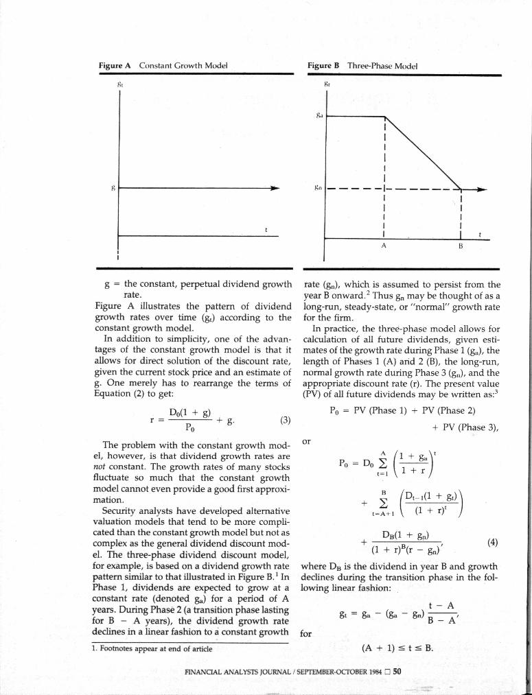
Figure A Constant Growth Model Figure B Three-Phase Model

g = the constant, perpetual dividend growthrate.

Figure A illustrates the pattern of dividendgrowth rates over time (gt) according to theconstant growth model.

In addition to simplicity, one of the advan-tages of the constant growth model is that itallows for direct solution of the discount rate,given the current stock price and an estimate ofg. One merely has to rearrange the terms ofEquation (2) to get:

Do(l + g)(3)

The problem with the constant growth mod-el, however, is that dividend growth rates arenot constant. The growth rates of many stocksfluctuate so much that the constant growthmodel cannot even provide a good first approxi-mation.

Security analysts have developed alternativevaluation models that tend to be more compli-cated than the constant growth model but not ascomplex as the general dividend discount mod-el. The three-phase dividend discount model,for example, is based on a dividend growth ratepattern similar to that illustrated in Figure B.' InPhase 1, dividends are expected to grow at aconstant rate (denoted ga) for a period of Ayears. During Phase 2 (a transition phase lastingfor B - A years), the dividend growth ratedeclines in a linear fashion to a constant growth

1. Footnotes appear at end of article

rate (gn), which is assumed to persist from theyear B onward.^ Thus gn may be thought of as along-run, steady-state, or "normal" growth ratefor the firm.

In practice, the three-phase model allows forcalculation of all future dividends, given esti-mates of the growth rate during Phase 1 (ga), thelength of Phases 1 (A) and 2 (B), the long-run,normal growth rate during Phase 3 (gn), and theappropriate discount rate (r). The present value(PV) of all future dividends may be written as:^

Po = PV (Phase 1) + PV (Phase 2)

+ PV (Phase 3),

or

DB(1 + gn)(1 + r)«(r - g j '

(4)

where DB is the dividend in year B and growthdeclines during the transition phase in the fol-lowing hnear fashion:

for

gt = ga - (ga - gn)

(A -I- 1) < t < B.

t - A

FINANCIAL ANALYSTS JOURNAL / SEPTEMBER-OCTOBER 1984 D 50

The three-phase model has several attributesthat make it popular with practitioners. First,because it assumes constant growth in Phase 3,the analyst does not have to estimate a perpetu-al stream of dividends. Instead, only five esti-mates are needed to calculate the stock price.Second, the model is much more flexible thanthe constant growth model, because it allowsfor some change in dividend growth rates overtime. Finally, although the necessary calcula-tions are fairly complex. Equation (4) may besolved by developing algorithms for use onprogrammable calculators or computers.'*

The three-phase model does have drawbacks,however. First, if Phases 1 and 2 cover morethan two or three years, solving for the pricebecomes tedious. Second, Equation (4) does notallow one to solve analytically for r; rather, onehas to "guess" at a discount rate, solve for Po,compare this figure with the current marketprice, then guess again using a higher (lower)discount rate if the calculated Po was higher(lower) than the current price. This iterativeprocess is continued until one arrives at a dis-count rate that results in a price that approxi-mates current market price.

Deriving the H-ModelConsider the "two-step" dividend growth ratepattern illustrated in Figure C. Initially, divi-dends grow at a constant rate of ga for A years.Thereafter, dividends grow at a constant rate ofgn. Given these assumptions, the present value

of the future dividend stream can be calculatedas:

or

.5

Po = PV (Step 1) + PV (Step 2),

t - A(1 + gn)'(1 + r)'

(5)

where DA is the dividend in year A.If we solve for the geometric progressions and

assume that r exceeds gn. Equation (5) may besimplified to:

Po =Do(l + ga)

I A - l

1 -gn

1 + r(6)

Equation (6) could be used to estimate Po, but ithas two drawbacks as a common stock valua-tion model. First, it is very tedious to solve for r,the discount rate, directly from Equation (6).Second, the dividend growth rate pattern as-sumed—that is, a constant growth rate for Ayears followed by a sudden jump to a long-run,normal growth rate—is highly unlikely.

A more realistic, yet operational, model isgiven by Equation (7), which approximatesEquation (6):

Figure C Two-Step Growth Rate Po = [(1 + gn) + A(ga - gn)]. (7)

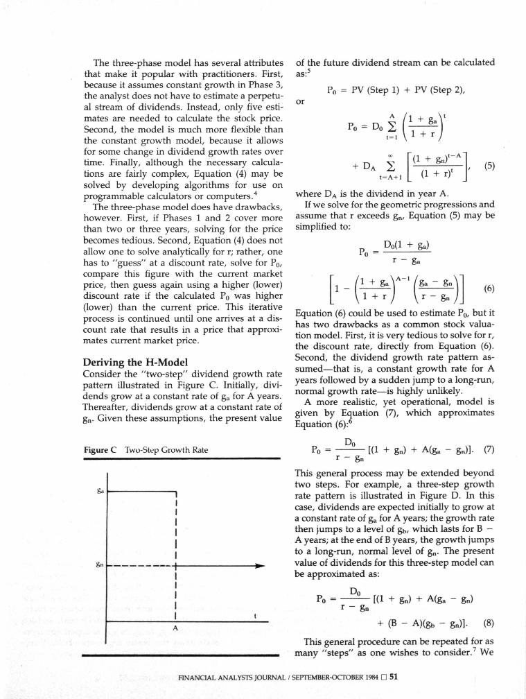
This general process may be extended beyondtwo steps. For example, a three-step growthrate pattern is illustrated in Figure D. In thiscase, dividends are expected initially to grow ata constant rate of ga for A years; the growth ratethen jumps to a level of gb, which lasts for B -A years; at the end of B years, the growth jumpsto a long-run, normal level of gn. The presentvalue of dividends for this three-step model canbe approximated as:

Po = ^— [(1 + gn) + A(ga - gn)gn

+ ( B - A)(gb- gn)]. (8)

This general procedure can be repeated for asmany "steps" as one wishes to consider.^ We

FINANCIAL ANALYSTS JOURNAL / SEPTEMBER-OCTOBER 1984 D 5 1

Figure D Three-Step Growth Rate

t

ga

8b

gn

k

A

111

1111 tB

will stop at three steps here, however, for tworeasons. First, increasing the number of stepsincreases the complexity of the model until itapproaches the complexity of Equation (1), thegeneral dividend discount model. As we addmore steps, we begin to defeat our purpose,which is to develop a simple and operationalmodel. Second, by making one additional as-sumption, we can inodify Equation (8) so that itis very similar to the three-phase model incurrent use and, at the same time, furthersimplify Equation (8).

To do this, assume that gb, the "middle step"growth rate, is exacfly halfway between ga andgn, SO that:

ga + gngb = ^ •

Substituting this into Equation (8) yields:

Do(1 + gn) +

A + B 1- gn) •

JNow substitute H for (A -I- B)/2, and we havethe H-model:

Po = [( + gn) + H(ga - gn)]. (9)

We have eliminated gb from the equation andhave to estimate only the beginning growth rate(ga) and the long-run growth rate (gn). We havemade H the "halfway" point for the period ofabove-normal growth.

Suppose, for illustration, that an analyst esti-

mates that XYZ Company, which has just paid aone dollar dividend, will experience a long-runnormal growth rate of 8 per cent and that theappropriate discount rate is 14 per cent. Theanalyst expects, however, that the growth ratewill be above normal for the next 10 years,starting out at 12 per cent and declining in alinear fashion until it reaches 8 per cent at theend of the 10 years. Because the total period ofabove-normal growth is 10 years, the halfwaypoint (H) is five years. The analyst thus has thefollowing estimates:

ga = 12%gn = 8%,r = 14%,Do = $1.00, andH = 5 years.

Using Equation (9), he can estimate the price forthe stock as follows:

Po =$1.00

0.14 - 0.08[1.08 + 5(0.12 - 0.08)]

= $21.33.

H-Model FeaturesThe H-model has several pleasing features.

There are no exponential terms; solving for Poinvolves only simple arithmetic. Also, to solveanalytically for the discount rate, the terms inEquation (9) have only to be rearranged asfollows:

= ^ [(1 +I 0

+ H(ga - gn)] + gn- (10)

If ga equals gn. Equation (10) reduces to Equa-tion (3) of the constant growth model. In anycase, solving for r by Equation (10) is straightfor-ward.

The H-model implies a growth rate patternover time that seems (to us at least) to beplausible for many firms.* Figure E illustratesthe implicit pattern. The growth rate, beginningat ga, declines in a steady fashion from ga to gnover a period of 2H years. The growth rate ishalfway between ga and gn at year H andreaches gn at the year 2H. (If ga is estimated tobe less than gn, then the line would slopeupwards toward gn over time.) This growth ratepattern seems more likely than a two or three-step pattern (Figures C and D) with suddenjumps from ga to gb to gn, and perhaps morelikely than the linear segments of the three-phase model (Figure B). 5? . ,

FINANCIAL ANALYSTS JOURNAL / SEPTEMBER-OCTOBER 1984 Q 52

Figure E H-Model Implicit Growth Rate Figure F H-Model vs. Tlirco-Phnso Model

8.1

I11. . ,

1111

11H

1

1111

1211

Analysts should also find the H-model intu-itively appealing. Suppose investors believethat a firm's normal growth rate is equal to gn,but believe that the firm currently has unusualinvestment opportunities and therefore willgrow at an above-normal rate for the next 2Hyears. In this case. Equation (9) of the H-modelindicates that the value of the stock is equal tothe capitalized value of the dividends assumingnormal growth (gn) plus the additional valuefrom the above-normal growth (ga). This inter-pretation becomes clearer if we rewrite Equation(9) as follows:

Do(l DoH(ga - gn)

>• - g n

The second term represents the incrementalvalue due to the temporary above-normalgrowth. Consider, for example, the case of XYZCompany. Using Equation (11), we can see thatits total price of $21.33 is composed of $18,000from normal growth prospects and $3.33 fromtemporary, above-normal growth, or:

Po =$1.00(1.08) $1.00(5)(0.12 - 0.08)

0.14 - 0.08 0.14 - 0.08

= 18.00 + 3.33 = $21.33.

Finally, the H-model is directly comparable tothe three-phase model. Both models require anestimate of the initial growth rate (ga), the long-run, normal growth rate (gn) and the discountrate (r). The three-phase model requires an

Sa + Sh2

Sn

.so

1111111A 1 )

—^^^ H-moiliI

\11111113

1

1111 t

2H

estimate of Phase 1 (A years) and Phase 2 (B-Ayears), whereas the H-model requires only anestimate of H—the halfway point.

Figure F compares the growth rate pattern ofthe three-phase model with the implicit growthrate pattern of the H-model. The H-model'sassumption that gb equals (ga-l-gn)/2 puts Hexactly halfway between the A and B of thethree-phase model. Thus H can be thought of ineither of two ways—(1) as one-half the timerequired for the firm's growth rate to declinefrom its initial level (ga) to the firm's long-runnormal growth rate (gn) or (2) as the pointhalfway through the transition phase (Phase 2)of the three-phase model.

As Equation (4) suggests, the three-phasemodel is relatively complex and requires either aprogrammable calculator or a computer, or a lotof time and patience. The H-model can besolved using simple arithmetic. In addition, theH-model can be used to solve analytically forthe discount rate, using Equation (10). By con-trast, the three-phase model requires an itera-tive process to solve for r. If the H-modelgenerates results that are similar to those of thethree-phase model, then it might be consideredas a replacement for the three-phase model.

H-Model ResultsTable I presents for six hypothetical cases

estimated prices generated by the H-model andthe three-phase model. In Case 1, ga, gn and restimates are 7, 4 and 9 per cent, respectively,for both models. For the three-phase model, A(the length of Phase 1) is estimated at five years

FINANCIAL ANALYSTS JOURNAL / SEPTEMBER-OCTOBER 1984 D 5 3

Table I H-Model vs. the Three-Phase Model

CaseNo.

123456

Common

gu

7%,1212

- 22020

Assumptions*

Q

4%44444

r

9%99999

/I

5yr.5yr.5yr.3yr.7yr.3yr.

Three-Phase

B

7yr.7yr.

15 yr.5yr.

13 yr.7yr.

Po

$23.9730.1737.6617.1268.1838.04

H-Model

H

6 yr.6 yr.

10 yr.4 yr.

10 yr.5yr.

Po

$24.4030.4036.8016.0052.8036.80

Ratio ofEstimated

Prices

0.980.981.021.071.291.03

* Do equals $1.00 in each case.

and B (the end of Phase 2) is estimated at sevenyears. The transition period, B-A, thus lasts fortwo years. Civen these assumptions, and theone dollar dividend assumption, the three-phase model generates a price of $23.97. The H-model, where H is set at six years (halfwaythrough the transition phase of the three-phasemodel), generates a price of $24.40.

In Case 2, the beginning growth rate assump-tion is increased to 12 per cent, while otherestimates remain the same. The results of thetwo models are again extremely close—$30.17for the three-phase model, versus $30.40 for theH-model. In Case 3, the transition period for thethree-phase model is lengthened to 10 years, sothat H, the halfway point of the H-model,becomes 10 years. Again, the answers generat-ed by the two models are similar—$37.66 versus$36.80.

Case 4 covers the possibility that the begin-ning growth rate is less than the long-run,normal growth rate. Although the answers gen-erated by the two models in this case are not asclose as in the first three cases, they are only$1.12 apart—$17.12 versus $16.00.

Case 5 illustrates the circumstances underwhich the two models will give answers that arenot reasonably close. This will occur when (1)there is a large difference between the begin-ning growth rate and the long-run, normalgrowth rate; (2) the time period over which theannual growth rates approach gn is relativelylong; and (3) the difference between the dis-count rate and the initial growth rate is relative-ly large.' In Case 5, the three-phase modelgenerates a price of $68.18, whereas the H-model generates a price of $52.80.

It seems unlikely that such a wide differencebetween the beginning growth rate and thelong-run growth rate—20 per cent versus 4 percent— would persist for very long. Over shorterperiods, however, such a difference may not be

uncommon. Case 6 shows that, under theseconditions, the two models provide very similarprices—$38.04 versus $36.80.

Under most plausible circumstances, then,the two models provide price estimates that areremarkably similar. This is borne out by the lastcolumn of Table I, which presents the ratio ofthe prices generated by the two models. Withthe exception of Case 5, the ratios are close to1.0, indicating that the prices are within a fewpercentage points of one another.'°

Using the H-ModelTo see exactly how the H-model might be usedto identify under or overpriced stocks, considerthe case of IBM. In February 1982, IBM wasselling for $62 per share. At that time. ValueLine was forecasting a dividend growth rate of12 per cent for IBM for the next five years. ValueLine does not publish estimates of long-run,normal growth rates or transition periods, butwe will assume that IBM's long-run, normaldividend growth rate is 7 per cent, or slightlyabove the average growth rate for industrialstocks." We'll further assume that its growthrate will decline from 12 to 7 per cent over aperiod of 22 years, so that the halfway point, H,is 11 years. We thus have:

ga = 12%,gn = 7%, andH = 11.

To determine the appropriate discount rate,or the "required return," we'll use the followingSecurity Market Line:'"^

' required r = 10% -I- 6%. (12)

Using Value Line's estimate of IBM's beta in1982—0.95—gives us a required return of 15.7per cent. Given these estimates and IBM's 1981dividend of $3.44, the H-model gives us a pricefor IBM of $64.06. Comparing this model price

FINANCIAL ANALYSTS JOURNAL / SEPTEMBER-OCTOBER 1984 n 54

with the market price of $62 suggests that IBMwas slightly underpriced. Of course, differentestimates of the dividend growth rates and therequired return would yield different results.The H-model, like every other model, can be nobetter than the estimates used as inputs.

The H-model can also be used to determinethe cost of equity, or expected return. This is thereturn investors expect, given the current stockprice and their estimates of future dividendgrowth rates. For example, given the marketprice of $62 and the above estimates for IBM,the expected return for IBM would be 16.0 percent, based on Equation (10) of the H-model:

expected r =$3.44

$62[(1.07) + 11(0.12-0.07)]

0.07 = 0.160.

Calculating the cost of equity using the H-modelis straightforward. By contrast, the same calcu-lation using the three-phase model requires aniterative process and, for all practical purposes,a computer.

Finally, the H-model allows investors to cal-culate security alphas—i.e., the difference be-tween the expected return and the requiredreturn. IBM's alpha would be calculated asfollows:

IBM alpha = 16.0% - 15.7% = -hO.3%.

The positive alpha is consistent with the earlierconclusion that IBM was slightly underpriced.

We hope the H-model will prove to be auseful addition to the analyst's tool kit. Like anyother tool, however, it is only of value whenproperly used. Without sound estimates ofgrowth rates and required returns, the H-modelcan provide little useful information. Withthem, it offers a theoretically sound and practi-cally efficient approach to stock valuation. •

Footnotes

1. The three-phase model has been proposed in theliterature by Nicholas Molodovsky, CatherineMay and Sherman Chottiner, "Common StockValuation—Principles, Tables, and Applica-tions," Financial Analysts Journal, March/April1965; W. Scott Bauman, "Investment Returns andPresent Values," Financial Analysts Journal, No-vember/December 1969; and Russell J. Fuller,"Programming the Three-Phase Dividend Dis-count Model," Journal of Portfolio Management,Summer 1979.

2. The growth rate during Phase 1 (ga) does nothave to be greater than the constant, steady-stategrowth rate (gn) assumed for Phase 3. If gnexceeds ga, then the growth rate increases in alinear fashion from ga to gn during Phase 2, thetransition phase. However, gn does have to beless than r; otherwise, the stock price would beinfinite because dividends would be growing at afaster rate than the rate at which they are beingdiscounted.

3. For the derivation of the three-phase model, seeFuller, "Programming the Three-Phase DividendDiscount Model," op dt.

4. Ihid.5. This two-step model has been presented previ-

continued

^Beneficiar220th ConsecutiveQuarterlyCommon StockDividendBeneficial Corporation hasannounced per share dividendspayable June 30, 1984 tostockholders of record at theclose of business June 4, 1984.

Common Stock —Quarterly —$.50

5% Cumulative PreferredStock — Semi annual — $1.25

$4.50 Dividend CumulativePreferred Stock — Semi-annual-$2.25

Payable July 31, 1984 to stock-holders of record at the close ofbusiness July 6,1984.

$5.50 Dividend CumulativeConvertible Preferred Stock —Quarterly - $1,375

May 23,1984

Beneficial corporation

HNANCIAL ANALYSTS JOURNAL / SEPTEMBER-OCTOBER 1984 Q 5 5

ously in the literature in an attempt to provide acommon stock valuation model that is more real-istic than the constant growth model. See J. FredWeston and Eugene F. Brigham, Managerial Fi-nance (Hinsdale, 111.: The Dry den Press, 1978),pp. 690-692.The formal derivation of the H-model as well asthe N-step model is available from the authors.The generalized N-step model is:

^ + X|(g,-gn) + X:{g:-gn) +

. . .+

where the "X"s represent the length of time foreach step.

8. In the process of deriving the H-model, the timedimension was suppressed. (Note there is nosubscript t in Equation (9)). Thus there is only animplicit growth rate pattern over time in the H-model. However, it can be shown that the implic-it growth rate pattern begins at g., and declines(or rises) in a linear fashion, reaching gn at thepoint in time of 2H, as Figure E illustrates.

9. If a discount rate of 15 per cent is used in Case 5,the difference between g , and r is 0.05(0.20-0.15) instead of 0.11 (0.20-0.09). Underthese circumstances, the three-phase model pricewould be $25.98, the H-model price would be

$24.00, and the ratio of the two would be 1.08.Thus if the difference between ga and r is relative-ly small, the results of the two models are similar,even if there is an unusually large differencebetween ga and gn and the transition period isrelatively long.

10. If, as in Case 5, ga is much greater than r and gaapproaches gn over a long time period, then thethree-phase model will always generate answersthat are substantially larger than the H-model's.Under these circumstances, the analyst will haveto decide which growth rate pattern most closelyresembles the pattern he foresees for the firm'sdividend stream.

11. Most studies of historical stock returns havefound the average dividend growth rate to be inthe 4 to 5 per cent range over the period from1926 to the late '70s. We increased this to 7 percent for IBM to adjust for a higher long-run stateof inflation and slightly better long-run prospectsfor IBM than the typical stock.

12. Historically, the Security Market Line has aver-aged approximately a 4 per cent intercept (rough-ly the risk-free rate) and a 5 per cent risk premi-um, where risk is measured in terms of beta.Thus the typical stock has averaged approximate-ly a 9 per cent return in the past. To adjust forcurrent market conditions, we increased the risk-free rate to 10 per cent and the risk premium to 6per cent.

Pension Fund Perspectivecontinued trom page 17

In June, Congressman TimothyWirth (Democrat, Colorado) intro-duced legislation that incorporatesmany recommendations of the Securi-ties and Exchange Commission (SEC).The bill would (1) prohibit companiesfrom making tender offers for theirown stock as a defense in a hostiletakeover attempt; (2) bar target compa-nies from issuing "golden parachutes"during a tender offer period; (3) forbidtarget companies from issuing a newclass of securities or more than 5 percent of a class or securities affectingmore than 5 per cent of the votingrights; and (4) require shareholder ap-proval if a company wants to buy backstock at a premium price from an in-vestor holding more than 3 per cent ofthe stock.

These moves will help to prevent

corporate managements from actingagainst the interests of shareholders,but they don't go far enough. If thetrustees of the Grumman pensionfund had served jail terms and if cor-porate managements involved inshareholder suits could be held per-sonally liable for damages and legalexpenses, we would probably see few-er incidents of the use of pension andcorporate assets to defeat tender offersand possible proxy fights. Finally, theconversions to two classes of securitiesfor voting purposes should be out-lawed by the SEC; otherwise the pro-posed rule changes will have little ef-fect. It goes against the fundamentaltenets of capitalism to strip investorsof their voting rights without compen-sation. If a family or managementgroup wants to ensure control, theymay buy over 50 per cent of the com-mon stock.

Takeovers and Shareholders: TheMounting Controversy . . . T. BoonePickens, Robert A. G. Monks, DeanLeBaron and other important speakerstell you how they did it, what youshould do about it, and what it allmeans . . . On Tuesday, October 30,1984 . . . The Waldorf Astoria Hotel. . . New York City . . . A one-dayconference sponsored by the FinancialAnalysts Federation. . . .

Call (212) 957-2869 for RegistrationInformation

FINANCIAL ANALYSTS JOURNAL / SEPTEMBER-OCTOBER 1984 D 5 6