Embed Size (px)
Citation preview
RURAL HEALTH SERIES Number 4
Rural, regional and remote
health
A guide to remoteness classifications
March 2004
Australian Institute of Health and Welfare Canberra
AIHW Catalogue Number PHE 53

© Australian Institute of Health and Welfare 2004
This work is copyright. Apart from any use as permitted under the Copyright Act 1968, no part may be reproduced without written permission from the Australian Institute of Health and Welfare. Requests and enquiries concerning reproduction and rights should be directed to the Head, Communication and Public Affairs, Australian Institute of Health and Welfare, GPO Box 570, Canberra ACT 2601.
This publication is part of the Australian Institute of Health and Welfare’s Rural Health Series. A complete list of the Institute’s publications is available from the Publications Unit, Australian Institute of Health and Welfare, GPO Box 570, Canberra ACT 2601, or via the Institute’s web site (http://www.aihw.gov.au).
ISSN 1448-9775 ISBN 1 74024 369 2 Suggested Citation Australian Institute of Health and Welfare 2004. Rural, regional and remote health: a guide to remoteness classifications. AIHW cat. no. PHE 53. Canberra: AIHW.
Australian Institute of Health and Welfare Board Chair Dr Sandra Hacker
Director Dr Richard Madden
Any enquiries about or comments on this publication should be directed to:
Labour Force and Rural Health Unit Australian Institute of Health and Welfare GPO Box 570 Canberra ACT 2601 Phone: (02) 6244 1154 Email: [email protected]
Published by Australian Institute of Health and Welfare
Printed by Union Offset
iii
Contents List of tables ........................................................................................................................................ iv
List of figures ....................................................................................................................................... v
Acknowledgments.............................................................................................................................. vi
Abbreviations.....................................................................................................................................vii
Explanatory notes ............................................................................................................................ viii
Geography ..................................................................................................................................viii
Terminology ...............................................................................................................................viii
Foreword ................................................................................................................................................x
Introduction...........................................................................................................................................1
The remoteness classifications...........................................................................................................2
Remoteness classifications—an overview..................................................................................2
Methodological differences ..........................................................................................................3
RRMA..............................................................................................................................................4
ARIA................................................................................................................................................6
ASGC Remoteness Areas............................................................................................................11
Strengths and weaknesses of the three methodologies and classifications............................13
Strengths and weaknesses of RRMA ........................................................................................13
Strengths and weaknesses of ARIA ..........................................................................................15
Strengths and weaknesses of ASGC Remoteness Areas ........................................................16
The practical limitations of remoteness classifications ..............................................................18
The ravages of time .....................................................................................................................18 An interim fix for boundary changes................................................................................19
Funding and remoteness classifications ...................................................................................20
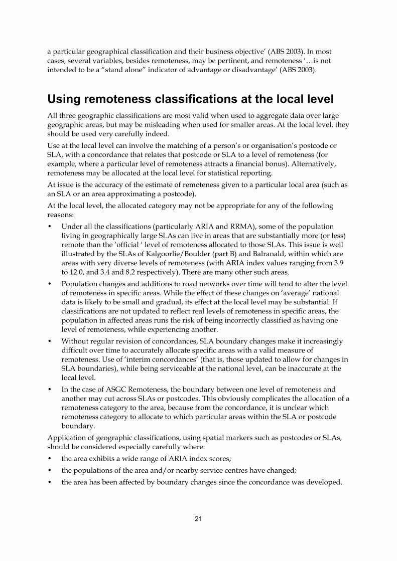
Using remoteness classifications at the local level..................................................................21
The geographical guide—SLAs and the three remoteness classifications ..............................23
Appendix A—Case studies of SLAs ...............................................................................................71
Appendix B—Interpolating ARIA and ARIA+ to a 1 km grid ..................................................75
Appendix C—Population distributions .........................................................................................76
References............................................................................................................................................77

iv
List of tables Table 1: Structure of the Rural, Remote and Metropolitan Areas (RRMA) classification.....5
Table 2: Structure of ARIA classification......................................................................................9
Table 3: Structure of ASGC Remoteness Areas .........................................................................11
Table 4: ASGC Remoteness Areas, ARIA and RRMA guide based on 2001 SLA boundaries—New South Wales....................................................................................26
Table 5: ASGC Remoteness Areas, ARIA and RRMA guide based on 2001 SLA boundaries—Victoria .....................................................................................................32
Table 6: ASGC Remoteness Areas, ARIA and RRMA guide based on 2001 SLA boundaries—Queensland ..............................................................................................38
Table 7: ASGC Remoteness Areas, ARIA and RRMA guide based on 2001 SLA boundaries—South Australia........................................................................................53
Table 8: ASGC Remoteness Areas, ARIA and RRMA guide based on 2001 SLA boundaries—Western Australia ...................................................................................57
Table 9: ASGC Remoteness Areas, ARIA and RRMA guide based on 2001 SLA boundaries—Tasmania ..................................................................................................62
Table 10: ASGC Remoteness Areas, ARIA and RRMA guide based on 2001 SLA boundaries—Northern Territory ..................................................................................64
Table 11: ASGC Remoteness Areas, ARIA and RRMA guide based on 2001 SLA boundaries—Australian Capital Territory and Other Territories............................67
Table 12: ASGC Remoteness Areas, ARIA and RRMA guide—selected SLAs ......................71
Table 13: Population estimates for remoteness classifications..................................................76

v
List of figures Figure 1: RRMA areas of Australia .....................................................................................................6
Figure 2: ARIA areas of Australia .....................................................................................................10
Figure 3: ASGC Remoteness Areas of Australia .............................................................................12
vi
Acknowledgments This report was commissioned by the Office of Rural Health (ORH) in the Department of Health and Ageing (DoHA), and guided by the members of the Rural Health Information Advisory Conmmittee (RHIAC). The following people contributed to this report by providing advice: • Frank Blanchfield (Geography Section, ABS), who provided the ASGC Remoteness
Areas map and provided expert feedback on the report, particularly regarding ASGC Remoteness Areas.
• Paul Nelson (DoHA), who produced the ARIA and RRMA maps and who provided expert feedback on the report, particularly regarding the ARIA classification.
• Phil Trickett (AIHW), who provided general advice on all three classifications. The geographic guide (Tables 4–11) is based on concordances developed and provided by the Australian Bureau of Statistics (ASGC Remoteness Areas) and the Department of Health and Ageing (ARIA). The original (1991) RRMA concordance, on which the 2001 concordance is based, was developed by the Department of Primary Industries and Energy and the then Department of Human Services and Health. This document was developed and prepared by Brendan Brady and Andrew Phillips.

vii
Abbreviations ABS Australian Bureau of Statistics AIHW Australian Institute of Health and Welfare ARIA Accessibility/Remoteness Index of Australia ASGC Australian Standard Geographical Classification AUSLIG Australian Surveying and Land Information Group CD Census Collection District DHAC Department of Health and Aged Care DHSH Department of Human Services and Health DoHA Department of Health and Ageing DPIE Department of Primary Industries and Energy GIS Geographic Information System GISCA National Key Centre for Social Applications of Geographic Information
Systems RRMA Rural, Remote and Metropolitan Areas SLA Statistical Local Area
Symbols used in the tables and figures . . not applicable n.a. not available n.p. not published in this report n.e.d. not elsewhere described
viii
Explanatory notes
Geography Capital City Statistical Division—represents the city in a broad sense. It should contain the anticipated development of the city for a period of at least 20 years (ABS 2003). Census Collection District (CD)—an area that one census collector can cover for distribution and collection of census forms, in a ten-day period. In urban areas this translates to approximately 200 dwellings, and fewer than this in areas of lower population densities. The CD is the smallest spatial unit in the ASGC (ABS 2002). In census years CDs aggregate up to Statistical Local Areas (SLAs). Populated Localities—based on AUSLIG ‘Populated Centres’ (DHAC & GISCA 2001). ‘These are mapped places, across Australia, from where people might need to travel to obtain services’ (ABS 2001a). Service Centres—are ABS-defined urban centres. An urban centre is a population cluster of 1,000 or more people. Urban centre boundaries are based on CDs (ABS 2002). Statistical Subdivision—a general purpose spatial unit. It can be made up of one or more SLAs (ABS 2002). Statistical Local Areas (SLAs)—based on the administrative areas of local government where these exist. Where there is no incorporated body of local government, SLAs are defined to cover the unincorporated areas. The SLA ‘is the base spatial unit used by the Australian Bureau of Statistics (ABS) to collect and disseminate statistics other than those collected in Population Censuses’ (ABS 2002).
Terminology Several terms have been used in this publication when describing the three classifications and their underlying methodologies. Some of these terms are explained further in ‘The remoteness classifications’ (see page 2). The following is a guide to how each term has been used in this publication.
Concordance—a tool that shows the correspondence between geographic areas (such as SLAs and postcodes) and the classes assigned under a given classification scheme.
Terms relating to the RRMA classification: RRMA classification—refers to the categoric classification. This classification consists of three broad zones (metropolitan, rural and remote) and seven finer classes (see Table 1 on page 5). RRMA methodology—refers to the procedures used to allocate SLAs into RRMA zones and classes.
ix
Terms relating to the ARIA classification: ARIA classification—refers to the categoric classification. This classification consists of five ARIA classes (Highly Accessible, Accessible, Moderately Accessible, Remote and Very Remote) (see Table 2 on page 9). Each ARIA class is defined by a range of ARIA index values. ARIA index value—refers to a continuous variable (with values ranging from 0 to 12) assigned to populated localities. ARIA methodology—refers to the procedures that determine the ARIA index values of populated localities. Terms relating to ASGC Remoteness Areas: ASGC Remoteness Areas is based on ARIA+ methodology. ARIA+ methodology and ARIA methodology (the underlying methodology of the ARIA classification) are similar but have some differences. ASGC Remoteness Areas—refers to the categoric classification. This classification consists of six ASGC Remoteness Area classes (Major Cities, Inner Regional, Outer Regional, Remote, Very Remote and Migratory) (see Table 3 on page 11). Each ASGC Remoteness Area class (excluding Migratory) consists of a range of ARIA+ index values. ARIA+ index value—refers to a continuous variable (with values ranging from 0 to 15) assigned to populated localities. ARIA+/ARIA+ methodology—refers to the procedures that determine the ARIA+ index values of populated localities.

x
Foreword The development over the last decade of geographical classifications for Australia that describe areas in terms of relative remoteness has provided an opportunity to compare a wide range of health and welfare indicators across Australia’s major cities, regional and remote areas. This publication reviews the methodology behind the three major classifications that describe areas in this way—the RRMA (Rural, Remote and Metropolitan Areas) classification, the ARIA (Accessibility/Remoteness Index of Australia) classification and the ASGC (Australian Standard Geographical Classification) Remoteness Areas classification. This publication also summarises each classification’s strengths and weaknesses and describes how the classifications are applied to administrative and survey data. This publication also contains a tabular geographical guide (Tables 4–11) showing the class to which each Statistical Local Area (SLA) is assigned under each of the three classifications. Appendix A illustrates the application of the geographic classifications to ten selected SLAs.
1
Introduction Policy makers, researchers and the general community are interested in the ways that the lives of Australians vary according to where they live. For example: • There has been an increasing concern over a number of years about perceived difficulties
faced by Australians living outside major metropolitan centres in accessing services (DHAC & GISCA 2001).
• There has also been particular concern about possible differences in health, education, income and a range of other factors, between those living in and those living outside major metropolitan centres. For example, a newly released report, Rural, Regional and Remote Health: A Study on Mortality (AIHW 2003), showed that, during the period 1997–1999, the mortality rates for people in regional and remote areas were higher than for people in capital cities.
Analyses of such differences depend on the ability to classify areas according to their remoteness. Three major remoteness classifications are currently used: • the RRMA (Rural, Remote and Metropolitan Areas) classification • the ARIA (Accessibility/Remoteness Index of Australia) classification (based on ARIA
index values), and • ASGC (Australian Standard Geographical Classification) Remoteness Areas (based on
ARIA+ index values—an enhanced version of the ARIA index values). This publication reviews these three classifications, their methodologies, and their strengths and weaknesses, and describes how the classifications are applied to administrative and survey data. The major points made in this publication are as follows: • The methodologies underlying the ARIA classification and ASGC Remoteness Areas
provide a better measure of remoteness than does the methodology underlying the RRMA classification.
• Two approaches have been used to apply ARIA and ARIA+ index values to SLA boundaries—allocating a class to the SLA based on the unweighted mean of index values for gridpoints lying within the SLA, and population weighting the SLA based on the mean of the index values for CDs lying within the SLA. Each approach has its strengths and weaknesses.
• Concordances used to assign remoteness classes to SLAs can be somewhat imprecise due to boundary and population changes that occur between censuses.
• The validity of these remoteness classifications in a given application (say, describing statistics or allocating funding) is greatest when the issue of interest is affected only, or mainly, by remoteness. Caution is required when other influences (for example, socioeconomic status, health outcomes, Indigenous status and local town size) are thought to play a role in the issue of interest (this may be the case, for example when analysing death rates, retention of GPs, etc.—see page 20).
2
The remoteness classifications Remoteness can be interpreted as ‘access to a range of services, some of which are available in smaller and others in larger centres: the remoteness of a location can thus be measured in terms of how far one has to travel to centres of various sizes’ (DHAC & GISCA 2001). Since the early 1990s three geographic classifications, embodying concepts of remoteness, have been developed: the RRMA and ARIA classifications and ASGC Remoteness Areas. This section provides an overview of the three remoteness classifications and the major differences in their underlying methodologies. The classifications and their underlying methodologies are then explained in more detail.
Remoteness classifications—an overview RRMA, ARIA and ASGC Remoteness Areas are geographic classifications used to group areas with similar characteristics. These classifications have been used to describe regional differences in a range of issues (such as health outcomes). Approximate population distributions for the three classifications are provided in Appendix C (page 76).
RRMA RRMA is the oldest classification, developed in 1994 by the Department of Primary Industries and Energy, and the then Department of Human Services and Health (DPIE & DHSH 1994). The RRMA classification allocated each Statistical Local Area (SLA) within capital cities and metropolitan centres (having a population of 100,000 or more) to the Metropolitan zone. All other SLAs were allocated to either the Rural or Remote zone based on the SLA’s score on an ‘Index of remoteness’. The index score was calculated by combining a personal distance index (relating to the SLA’s population density) and distance indices (relating to the distance of the centroid of an SLA to the nearest urban centres in each of four categories). The SLA was then allocated a class (e.g. ‘small rural centres’) within the zone, based on the population of the urban centre within the SLA (DPIE & DHSH 1994). RRMA classifies SLAs as metropolitan (‘capital cities’ or ‘other metropolitan areas’), rural (‘large rural centres’, ‘small rural centres’ and ‘other rural areas’), and remote (‘remote centres’ and ‘other remote areas’). The RRMA measure of remoteness is based on population estimates from the 1991 census.
ARIA The ARIA classification was developed in 1997 by the then Commonwealth Department of Health and Aged Care, based on a continuous measure of remoteness (also called ARIA) developed by GISCA. In this classification, an ARIA category is allocated on the basis of the average ARIA index score (between 0 and 12) within an area (such as an SLA). The ARIA index score is based on the road distance from the closest service centres in each of four classes (as defined using 1996 census population data). ARIA index scores, and therefore ARIA categories, are capable of being updated over time as populations change. ARIA
3
categorises areas as ‘highly accessible’, ‘accessible’, ‘moderately accessible’, ‘remote’ and ‘very remote’.
ASGC Remoteness Areas ASGC Remoteness was released in 2001 by the ABS, and was based on an enhanced measure of remoteness (ARIA+) developed by GISCA. The ARIA+ index values (used in ASGC Remoteness Areas) and ARIA index values (used in the ARIA classification) of localities are calculated in a similar manner although there are some differences. For example: • ARIA+ index values (between 0 and 15) are based on road distance from a locality to the
closest service centre in each of five classes of population size (instead of four—as in ARIA).
• ASGC Remoteness categories are given to Census Collection Districts (CDs) on the basis of the average ARIA+ score within the CD. An assessment of remoteness in individual SLAs (or other areas) can then be made on the basis of the ASGC Remoteness Area categories allocated to the SLA’s constituent CDs.
ASGC Remoteness categorises areas as ‘major cities’, ‘inner regional’, ‘outer regional’, ‘remote’ and ‘very remote’.
Methodological differences Among the main differences between the methodologies underlying the three classifications are the following: • RRMA’s ‘Index of remoteness’ is based on distance to service centres as well as a
measure of ‘distance from other people’ (DPIE & DHSH 1994). ARIA and ARIA+ index values, however, are based on distance to service centres only.
• The ARIA/ARIA+ methodologies calculate distances from populated localities to service centres based on minimum road distance. The RRMA methodology uses ‘distance’ factors based on straight-line distance between the centroid of the SLA and the centroid of the nearest service centres, and ‘personal distance’ factors based on population density.
• The ARIA methodology calculates distance to the nearest centre in each of four categories of service centre, while the ARIA+ methodology calculates distance to the nearest centre in each of five categories of service centre.
• The ARIA and ARIA+ methodologies result in index values interpolated to points on a grid covering all of Australia, which are 1 km apart. This allows ARIA and ASGC Remoteness Area classes (or population-weighted concordances based on these classes) to be applied to SLAs or any other area. RRMA does not have this flexibility. The RRMA classification uses Statistical Local Areas (SLAs) as the basis for calculating and disseminating RRMA information. As such, the RRMA methodology and classification can be directly applied only to SLAs.
4
RRMA The RRMA classification was developed in 1994 by the Department of Primary Industries and Energy, and the then Department of Human Services and Health (DPIE & DHSH 1994). The RRMA classification was the first of the three to be developed, and was (and still is) used for research purposes and, in some cases, to allocate funding to areas.
RRMA methodology This is a brief summary of the processes undertaken in 1994 to allocate SLAs (based on 1991 boundaries) to RRMA zones and classes. 1. Each SLA in a capital city1 was allocated to the Metropolitan zone and to the RRMA
class of Capital cities. Each SLA in a metropolitan centre2 with a population equal to or greater than 100,000 was allocated to the Metropolitan zone and to the RRMA class of Other metropolitan centre.
2. An ‘Index of remoteness’ was constructed for the remaining SLAs by combining a personal distance index relating to the SLA’s population density3 and partial indices relating to the distance of the centroid of an SLA to the centroid of urban centres4 that were: − a capital city urban centre − an ‘other’ metropolitan urban centre (a non-capital city with a population equal to
or greater than 100,000) − a large urban centre (population 25,000 to 99,999), and − a small urban centre (population 10,000 to 24,999).
3. SLAs with an ‘Index of remoteness’ value less than or equal to 10.5 were allocated to the Rural zone. SLAs with an ‘Index of remoteness’ value greater than 10.5 were allocated to the Remote zone.5
4. The SLAs were then allocated to a RRMA class based on the population size of the urban centre within the SLA (see Table 1) (DPIE & DHSH 1994).
1 Based on Capital City Statistical Division boundaries—see page viii.
2 Based on Statistical Subdivision boundaries—see page viii.
3 The SLA’s population was based on place of usual residence counts on census night 1991.
4 Urban centre populations were based on place of enumeration counts on census night 1991. Place of usual residence counts for urban centres were not available (DPIE & DHSH 1994).
5 Note: where a larger centre is closer to a populated locality than a smaller centre, the smaller centre is ignored when calculating the index of remoteness for the SLA. This is because it is assumed that the goods and services available in the smaller centre are also available in the larger centre (DPIE & DHSH 1994).

5
RRMA classification The RRMA classification consists of three zones (Metropolitan, Rural and Remote) and seven classes (Table 1).
Table 1: Structure of the Rural, Remote and Metropolitan Areas (RRMA) classification
Zone Class Abbreviation
Metropolitan zone Capital Cities M1
Other Metropolitan Centres (urban centre population > 100,000) M2
Rural zone Large Rural Centres (urban centre population 25,000–99,999) R1
Small Rural Centres (urban centre population 10,000–24,999) R2
Other Rural Areas (urban centre population < 10,000) R3
Remote zone Remote Centres (urban centre population > 5,000) Rem1
Other Remote Areas (urban centre population < 5,000) Rem2
Source: DPIE & DHSH 1994.
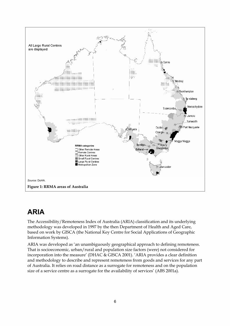
Figure 1 shows the geographic distribution of each RRMA class.
6
Source: DoHA.
Figure 1: RRMA areas of Australia
ARIA The Accessibility/Remoteness Index of Australia (ARIA) classification and its underlying methodology was developed in 1997 by the then Department of Health and Aged Care, based on work by GISCA (the National Key Centre for Social Applications of Geographic Information Systems). ARIA was developed as ‘an unambiguously geographical approach to defining remoteness. That is socioeconomic, urban/rural and population size factors (were) not considered for incorporation into the measure’ (DHAC & GISCA 2001). ‘ARIA provides a clear definition and methodology to describe and represent remoteness from goods and services for any part of Australia. It relies on road distance as a surrogate for remoteness and on the population size of a service centre as a surrogate for the availability of services’ (ABS 2001a).

7
ARIA methodology The ARIA methodology produces index values, between 0 and 12, for 11,340 populated localities. Areas with an ARIA index value of 0 have the highest levels of access to goods and services, and areas with an ARIA index value of 12 have the highest level of remoteness. The ARIA index value for a populated locality was calculated as follows, using the fictional populated locality of Kickatinalong as an example:
1. Service centres in Australia were allocated to four categories based on their population size in the 1996 census. A service centre, in this case, is defined as an urban centre with a population equal to or greater than 5,000. The four categories of service centre had populations of:
A. equal to or more than 250,000 persons, B. 48,000 to 249,999 persons, C. 18,000 to 47,999 persons, and D. 5,000 to 17,999 persons.
2. For each of the 11,340 populated localities the road distances to the closest category A, B, C and D service centres were calculated. For example, the distance of Kickatinalong from the closest category A service centre was 826 km.
3. The average distance was also calculated from all 11,340 populated localities to the nearest category A, B, C and D service centres. For example, the average distance of all populated localities to their nearest category A service centre (population > 250,000) is 413 km.
4. The distance calculated for a particular populated locality in step 2 was divided by the average distance for all populated localities in step 3 to give a ratio. For example, the ratio for Kickatinalong to category A service centres was 2.0 (that is, 826/413). The interpretation is that Kickatinalong was twice as far from a category A service centre as the average populated locality.
5. This ratio for each populated locality was capped at a value of 3.0. For example, if the distance of a populated locality from a category A service centre was four times the average distance of all populated localities to their nearest category A service centre, then the ratio would be 3.0.
6. For each populated locality, the ratios relating to each of the four categories of service centres (A, B, C and D) were summed to give an index value out of 12. For example, Kickatinalong was twice as distant from a category A service centre as the average distance of all populated localities to their nearest category A service centre, 2.8 times as far as the average from a category B centre and 0 times as far from a category C centre (Kickatinalong itself is a C centre) as the average. A category C centre is also assumed to have the same services as a category D centre. Therefore Kickatinalong was 0 times as far as the average from a category D centre.6 The sum of the four ratios (the ARIA index value) for Kickatinalong would have been 4.8 (that is, 2.0 + 2.8 + 0 + 0).
ARIA index values for Tasmania were calculated using an additional factor to account for the fact that it is separated from the nearest category A centre (Melbourne) by sea. A separate 6 Note: where a populated locality is closer to a larger centre than to a smaller centre, the ratio of the distance to the smaller centre is calculated as 0. This is because it is assumed that the goods and services available in the smaller centre are also available in the larger centre.
8
weighted distance measure was used to calculate ARIA index values for islands which are not accessible via land transport. ARIA index values for each populated locality were then interpolated to points on a grid covering all of Australia, which are 1 km apart. The interpolation to a grid is a necessary step before ARIA index values could be calculated for other spatial units (for example, CDs, SLAs or postcodes) (DHAC & GISCA 2001). The interpolation process is explained further in Appendix B.
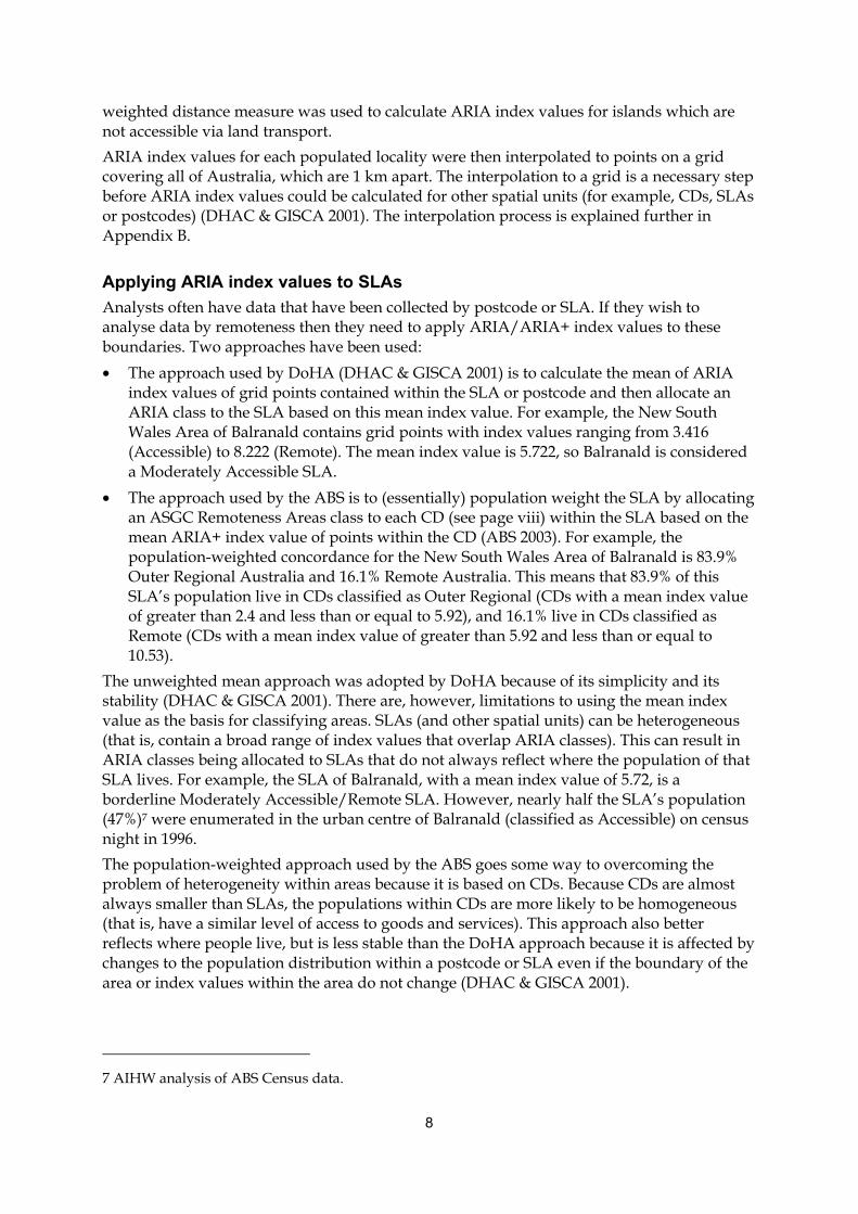
Applying ARIA index values to SLAs Analysts often have data that have been collected by postcode or SLA. If they wish to analyse data by remoteness then they need to apply ARIA/ARIA+ index values to these boundaries. Two approaches have been used: • The approach used by DoHA (DHAC & GISCA 2001) is to calculate the mean of ARIA
index values of grid points contained within the SLA or postcode and then allocate an ARIA class to the SLA based on this mean index value. For example, the New South Wales Area of Balranald contains grid points with index values ranging from 3.416 (Accessible) to 8.222 (Remote). The mean index value is 5.722, so Balranald is considered a Moderately Accessible SLA.
• The approach used by the ABS is to (essentially) population weight the SLA by allocating an ASGC Remoteness Areas class to each CD (see page viii) within the SLA based on the mean ARIA+ index value of points within the CD (ABS 2003). For example, the population-weighted concordance for the New South Wales Area of Balranald is 83.9% Outer Regional Australia and 16.1% Remote Australia. This means that 83.9% of this SLA’s population live in CDs classified as Outer Regional (CDs with a mean index value of greater than 2.4 and less than or equal to 5.92), and 16.1% live in CDs classified as Remote (CDs with a mean index value of greater than 5.92 and less than or equal to 10.53).
The unweighted mean approach was adopted by DoHA because of its simplicity and its stability (DHAC & GISCA 2001). There are, however, limitations to using the mean index value as the basis for classifying areas. SLAs (and other spatial units) can be heterogeneous (that is, contain a broad range of index values that overlap ARIA classes). This can result in ARIA classes being allocated to SLAs that do not always reflect where the population of that SLA lives. For example, the SLA of Balranald, with a mean index value of 5.72, is a borderline Moderately Accessible/Remote SLA. However, nearly half the SLA’s population (47%)7 were enumerated in the urban centre of Balranald (classified as Accessible) on census night in 1996. The population-weighted approach used by the ABS goes some way to overcoming the problem of heterogeneity within areas because it is based on CDs. Because CDs are almost always smaller than SLAs, the populations within CDs are more likely to be homogeneous (that is, have a similar level of access to goods and services). This approach also better reflects where people live, but is less stable than the DoHA approach because it is affected by changes to the population distribution within a postcode or SLA even if the boundary of the area or index values within the area do not change (DHAC & GISCA 2001).
7 AIHW analysis of ABS Census data.

9
ARIA classification ARIA index values have been ranged into ARIA classes (see Table 2). Continuing the earlier fictional example, the populated locality of Kickatinalong, with an ARIA index value of 4.8, would be classified as Moderately Accessible.
Table 2: Structure of ARIA classification
Class Abbreviation Index value range
Highly Accessible HA 0–1.84(a)
Accessible A >1.84–3.51(a)(b)
Moderately Accessible MA >3.51–5.80(c)
Remote R >5.80–9.08(d)
Very Remote VR >9.08–12(e)
(a) The cut-offs used are in practice slightly different from the values published by DoHA (DHAC & GISCA 2001) and presented here.
(b) Greater than 1.84 but less than or equal to 3.51.
(c) Greater than 3.51 but less than or equal to 5.80.
(d) Greater than 5.80 but less than or equal to 9.08.
(e) Greater than 9.08 but less than or equal to 12.
Source: DHAC & GISCA 2001.
The classes have been characterised broadly as follows: • Highly Accessible—relatively unrestricted accessibility to a wide range of goods and
services and opportunities for social interaction; • Accessible—some restrictions to accessibility of some goods and services and
opportunities for social interaction; • Moderately Accessible—significantly restricted accessibility of goods and services and
opportunities for social interaction; • Remote—very restricted accessibility of goods, services and opportunities for social
interaction; • Very Remote—very little accessibility of goods, services and opportunities for social
interaction (DHAC & GISCA 2001).
Figure 2 shows the distribution of SLAs in each ARIA class based on the mean index values of 1996 SLA boundaries.

10
Source: DoHA.
Figure 2: ARIA areas of Australia
11
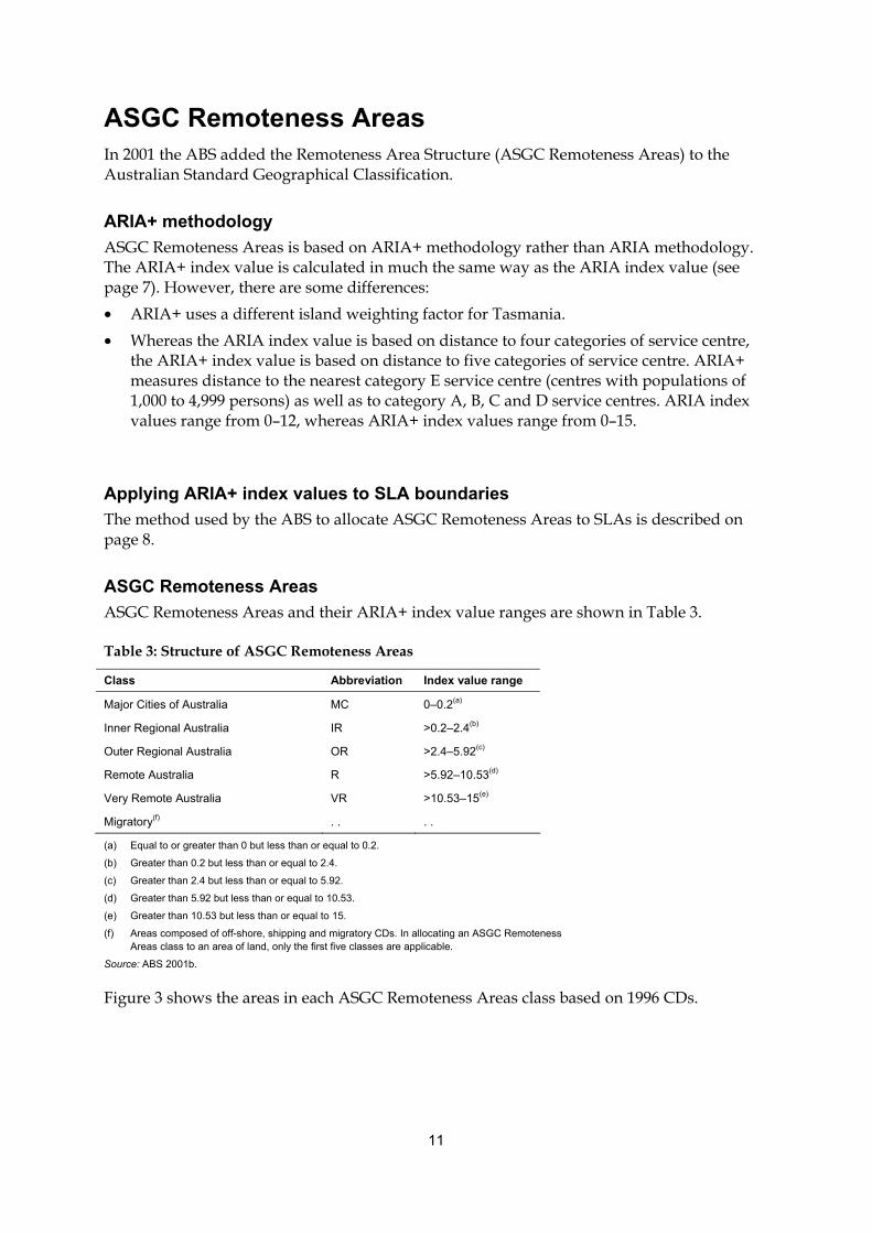
ASGC Remoteness Areas In 2001 the ABS added the Remoteness Area Structure (ASGC Remoteness Areas) to the Australian Standard Geographical Classification.
ARIA+ methodology ASGC Remoteness Areas is based on ARIA+ methodology rather than ARIA methodology. The ARIA+ index value is calculated in much the same way as the ARIA index value (see page 7). However, there are some differences: • ARIA+ uses a different island weighting factor for Tasmania. • Whereas the ARIA index value is based on distance to four categories of service centre,
the ARIA+ index value is based on distance to five categories of service centre. ARIA+ measures distance to the nearest category E service centre (centres with populations of 1,000 to 4,999 persons) as well as to category A, B, C and D service centres. ARIA index values range from 0–12, whereas ARIA+ index values range from 0–15.
Applying ARIA+ index values to SLA boundaries The method used by the ABS to allocate ASGC Remoteness Areas to SLAs is described on page 8.
ASGC Remoteness Areas ASGC Remoteness Areas and their ARIA+ index value ranges are shown in Table 3.
Table 3: Structure of ASGC Remoteness Areas
Class Abbreviation Index value range
Major Cities of Australia MC 0–0.2(a)
Inner Regional Australia IR >0.2–2.4(b)
Outer Regional Australia OR >2.4–5.92(c)
Remote Australia R >5.92–10.53(d)
Very Remote Australia VR >10.53–15(e)
Migratory(f) . . . .
(a) Equal to or greater than 0 but less than or equal to 0.2.
(b) Greater than 0.2 but less than or equal to 2.4.
(c) Greater than 2.4 but less than or equal to 5.92.
(d) Greater than 5.92 but less than or equal to 10.53.
(e) Greater than 10.53 but less than or equal to 15.
(f) Areas composed of off-shore, shipping and migratory CDs. In allocating an ASGC Remoteness Areas class to an area of land, only the first five classes are applicable.
Source: ABS 2001b.
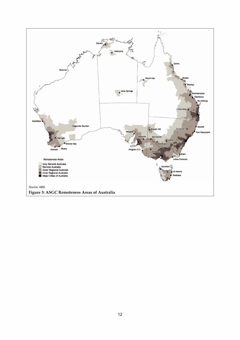
Figure 3 shows the areas in each ASGC Remoteness Areas class based on 1996 CDs.
12
Source: ABS.
Figure 3: ASGC Remoteness Areas of Australia
13
Strengths and weaknesses of the three methodologies and classifications Each remoteness classification and its underlying methodology has its advantages and disadvantages depending on how it is used. All of these classifications are useful for differentiating between areas with different levels of generalised remoteness (in the case of the ARIA classification and ASGC Remoteness Areas) and between areas with both different levels of remoteness and different local town sizes (in the case of RRMA).
Strengths and weaknesses of RRMA The release of the RRMA classification in 1994 was significant in that it was the first time that a remoteness classification was made widely available, applied to administrative and survey data and used in the allocation of funding to areas. Its widespread acceptance and usage, over the past decade, by a number of organisations has been an important step in the development of more precise measures of remoteness (classifications based on ARIA and ARIA+ methodologies). The RRMA classification was the only widely available remoteness classification from 1994 until 1999 (when the ARIA classification was released).
Strengths and weaknesses of RRMA methodology RRMA’s widespread acceptance and usage has been due to several factors: • All areas within an SLA boundary are given the same remoteness class. This makes
RRMA a simple tool to use for both research purposes and in allocating funding to SLAs. • The three zones (Metropolitan, Rural and Remote) are fairly logical groupings of areas
within Australia. These zones exhibit differences in relation to service and infrastructure provision, economic base, land use, natural resources, demography and social structure (DPIE & DHSH 1994).
The RRMA methodology does, however, have a number of weaknesses, compared to the ARIA and ARIA+ methodologies. The RRMA methodology is a ‘rougher’ measure of remoteness than the ARIA and ARIA+ methodologies because it: • is based on SLAs. All areas within the SLA boundary are assigned the same remoteness
class even though some SLAs are, in fact, heterogeneous in terms of remoteness (that is, they contain populations with widely varying levels of access to goods and services). ARIA and ARIA+ index values are built up from grid points rather than being based on fixed geographical boundaries;
• uses the centroid of the SLA as the reference point for calculating distance to service centres. The use of the SLA’s centroid can be a source of error in calculating distance to service centres because most people may, in large SLAs, live some distance from the

14
centroid. The ARIA and ARIA+ methodologies are based on distance from populated localities to service centres and this is more reflective of where people actually live;
• uses an ‘Index of remoteness’ derived from indices based on straight-line distance from the centroid of the SLA to the centroid of the nearest urban centres within each population category. For example, the centroid of an SLA may be 50 km from a large urban centre ‘as the crow flies’; however, the road distance to that centre could be twice the distance. The distance measure used in the ARIA and ARIA+ methodologies is preferable because it is based on actual road distance between a populated locality and its nearest service centres (DHAC & GISCA 2001);
• uses an ‘Index of remoteness’ based on population density as well as distance measures to distinguish between rural and remote SLAs (ARIA and ARIA+ index values are based on distance measures alone). Although population density can provide an indication of the ‘urban-ness’ of an area, the results can become relatively meaningless when applied to spatial units, such as SLAs, which vary widely in physical size. For example, in 1991 the Cities of Broken Hill and Kalgoorlie/Boulder both contained urban centres with similar sized populations. The boundary of Broken Hill City approximated the boundary of the urban centre of Broken Hill. In contrast the boundary of Kalgoorlie/Boulder City stretched from the urban centre of Kalgoorlie/Boulder to the Western Australia/South Australia border. The difference in population densities contributed to Broken Hill City being designated as a Rural SLA and Kalgoorlie/Boulder City as a Remote SLA.
Strengths and weaknesses of the RRMA classification
The RRMA classification also has the following weaknesses in comparison to the ARIA classification and ASGC Remoteness Areas:
• Although a measure of remoteness is used to distinguish between rural and remote SLAs, the RRMA classification itself does not compare the relative level of accessibility/remoteness of each Rural and each Remote SLA. Instead, it uses the population of urban centres within an SLA to distinguish between remoteness classes. Thus an SLA classified as an ‘Other rural area’ is not necessarily more remote than an SLA classified as a ‘Small rural centre’ or a ‘Large rural centre’. The classes in the ARIA classification and ASGC Remoteness Areas, on the other hand, are based on a remoteness measure (that is, ranges of ARIA and ARIA+ index values), rather than the urban centre population. Therefore it can be said that under the ARIA classification a Moderately Accessible locality is more remote than an Accessible locality and, under ASGC Remoteness Areas, a locality in Outer Regional Australia is more remote than a locality in Inner Regional Australia.
• In the RRMA classification, ‘Capital cities’ are based on Capital City Statistical Divisions (see page viii). Thus there is no differentiation between people living closer to the middle of a capital city and those living on the outskirts. Under ASGC Remoteness Areas, however, some parts of the outer suburban SLAs are classed as Inner Regional Australia, reflecting the lower level of access to goods and services experienced by people living in these areas compared to people living closer to the city centre.
• Under the RRMA classification, all capital cities are classed as ‘Capital cities’ regardless of the population size and relative remoteness of the individual cities. Under this classification, Darwin (population of approximately 70,000 and surrounded by sparsely
15
populated areas), and Hobart (population of approximately 125,000) are placed in the same class as Sydney (with a population of more than 4 million).
Strengths and weaknesses of ARIA Strengths and weaknesses of ARIA methodology The ARIA methodology has a number of advantages over the RRMA methodology: • The ARIA methodology is conceptually simpler than the RRMA methodology in that it
measures remoteness only in geographic terms whereas RRMA’s ‘Index of remoteness’ combines a distance measure with a population density measure.
• The ARIA methodology uses the point location of towns and measures the distance of populated localities to the nearest of each category of service centre by road, whereas RRMA’s ‘Index of remoteness’ uses a straight line measure from the centroid of the SLA to the closest of each category of service centre.
• The ARIA index values of an area are less likely to change over time than the RRMA class of an area. The ARIA index value of a populated locality will only change when the population in one or more of the four service centres changes significantly, resulting in a reclassification to a different service category. This robustness is enhanced by the wide range in population size defining each service centre category, and the fact that service centres with populations under 5,000 people are not included in the calculation of ARIA index values. (DHAC & GISCA 2001). The RRMA class of an area can also be affected by population changes in nearby service centres and by boundary changes. Additionally, the RRMA class of an area should change if the population of the urban centre within the SLA breaches a class threshold. For example, if an urban centre within a rural SLA increased in population from below 10,000 to above 10,000 then the RRMA class for this SLA would need to change from Other rural area (R3) to Small rural centre (R2).
A weakness in the ARIA methodology is that it can sometimes result in highly dissimilar areas being given the same remoteness score. For example, in 1999, the City of Dubbo and the shire of Urana (with populations of 36,701, and 1,497 respectively in 1996) had almost identical ARIA scores (2.82) and were therefore included in the same ARIA class (Accessible). The City of Dubbo was in this class mainly because it is a large regional centre, whereas Urana is in this class mainly as a result of its moderate proximity (approximately 100 km by road) to Wagga Wagga and Albury. Accessibility of health professionals and other issues affecting health in each of these two areas would likely be quite different. This is less of a problem in the methodologies underlying the RRMA and ASGC Remoteness classifications. In RRMA, the population size of the urban centre within the SLA is also taken into consideration. In ASGC Remoteness, ARIA+ better differentiates in regional and remote areas because it also reflects distance to the small service centres. Additionally, ASGC Remoteness Areas are based on the average ARIA+ score in CDs (rather than the larger SLAs). The ARIA methodology is a purely geographical methodology based on distance measures. This is a strength of the ARIA methodology but also a limitation. This pure approach means that the methodology has to work with a number of assumptions which may not always be accurate. Two such assumptions relate to levels of car ownership and road conditions. Firstly, it is assumed that persons living in an area have access to road transport. While car ownership in Australia is widespread, some population groups, such as persons in rural areas (where, in addition, public transport can be lacking or limited) have lower levels of
16
access to road transport than the general population. Secondly, the ARIA methodology does not allow for differences in terms of road quality and road serviceability in calculating distance to service centres. For example, the remote Northern Territory community of Nhulunbuy is without road access for substantial parts of the year due to flooding (ABS 2001b). It should be noted that access to transport and road quality are also not addressed in either the RRMA or ARIA+ methodologies.
Strengths and weaknesses of the ARIA classification A strength of the ARIA classification, in comparison to the RRMA classification, is that it differentiates between areas in terms of levels of accessibility/remoteness. Moderately Accessible areas are less accessible than Accessible areas but more accessible than Remote areas. Although the RRMA methodology allocates SLAs into Metropolitan, Rural and Remote zones the RRMA classification does not however describe the differing levels of accessibility/remoteness of SLAs within each zone, except by reference to the size of the population in the local town. A disadvantage of the ARIA classification is the broadness of the range of index values of the non-remote classes. The class definitions used for the non-remote classes in the ARIA classification are broader than those used in ASGC Remoteness Areas. For example, the ARIA class ‘Highly Accessible’ includes metropolitan fringe areas and many regional centres whereas the ASGC Remoteness Area class of ‘Major Cities of Australia’ does not tend to include metropolitan fringe areas or any of the regional centres. The broadness of the ARIA classes therefore prevents comparisons between metropolitan, metropolitan-fringe and regional centre populations. The application of different cut-off index values to the continuous ARIA index would yield a version of the ARIA classification similar (but by no means identical) to ASGC Remoteness Areas. Another disadvantage of the ARIA classification is that it defines 81% of the population as living in the most accessible class (Highly Accessible areas). This leaves 19% of the population to be shared between the other four areas, making statistical comparisons less reliable because of small population sizes in these areas. In ASGC Remoteness Areas only 66% of the population are allocated to the most accessible ASGC Remoteness Areas class (Major Cities of Australia), providing scope for greater statistical discrimination in areas outside this class.
Strengths and weaknesses of ASGC Remoteness Areas ASGC Remoteness Areas classification is based on ARIA+ index values, rather than ARIA index values. ARIA+ has all of the advantages of the ARIA methodology (see ‘Strengths and weaknesses of ARIA methodology’ on page 15) as well as some additional advantages.
Strengths and weaknesses of ARIA+ methodology In ARIA+, average distance is calculated from each populated locality to category E service centres (centres with a population of 1,000 to 4,999 persons) as well as to the four types of service centre used in the ARIA methodology. This gives ARIA+ a greater level of precision in its measurement of remoteness than the ARIA methodology (particularly in the more remote areas). However with the additional 545 (category E) towns on the list of reference
17
service centres, it is more likely that population change over time will result in the re-categorisation of service centres, creating a need to update the ARIA+ index values of an area. Thus ARIA+ index values are less stable over time than ARIA index values, particularly in remote areas (however, as a consequence, they may better reflect actual levels of remoteness at any time). The ARIA+ methodology has the same weaknesses as the ARIA methodology (see ‘Strengths and weaknesses of ARIA methodology’ on page 15).
Strengths and weaknesses of ASGC Remoteness Areas An advantage of the ASGC Remoteness Areas classification is that it defines the least remote areas more tightly than the ARIA classification because it has a lower cut-off index value for the least remote area. For example almost 8% of the population of the outer Sydney SLA of Baulkham Hills and 24% of the population of the outer Perth SLA of Mundaring live in CDs classified as Inner Regional Australia. This acknowledges the likelihood that outer suburban areas would have lower levels of access to goods and services than areas closer to the Central Business District. In the ARIA classification these two SLAs are classed as Highly Accessible, as are regional centres such as the Cities of Tamworth, Orange and Wagga Wagga. An advantage of this classification over the RRMA classification is that it does not include the least accessible of the capital cities in the least remote class. Areas within Hobart are classed as Inner Regional Australia and areas in Darwin are classed as Outer Regional Australia because these capital cities are not category A service centres (service centres with populations of equal to or more than 250,000 persons) in their own right. Although ASGC Remoteness Areas defines the least remote classes more closely than the RRMA and ARIA classifications, the classification is not perfect. The cut-off index values used to distinguish between each ASGC Remoteness Areas class are ‘relatively arbitrary’ (as they are in the ARIA classification). ASGC Remoteness Areas groups areas that have similar, but not identical, characteristics of remoteness (ABS 2003).
18
The practical limitations of remoteness classifications Certain limitations have been identified in relation to the use of remoteness classifications: • Boundary and population changes can make concordances based on remoteness
classifications less precise over time and this can affect the quality of data that is cross-classified by remoteness, particularly data collected during the years between the censuses.
• Remoteness classifications only indicate relative levels of accessibility to goods and services. As such, their effectiveness as a means of determining funding to non-metropolitan areas may be limited (page 20).
• Use of any of the three classifications at the local level should be cautious (page 21). Changes to the boundaries of administrative areas such as SLAs, population change affecting real levels of remoteness within an SLA, and the wide range of levels of remoteness within some SLAs could adversely affect the accuracy of the perceived level of remoteness for at least some residents within an SLA.
The ravages of time The fictional SLA of Kickatinalong would always be classified as an ‘Other Rural Area’ under the RRMA classification, as ‘Moderately Accessible’ under the ARIA classification, and as ‘Outer Regional Australia’ under ASGC Remoteness Areas if: • the population in this area (and surrounding areas—including the major metropolitan
centres) remained the same; • new roads were never built (and old roads were maintained); and • Kickatinalong’s boundary did not change. Such a situation would rarely, if ever, occur and there are a number of scenarios that could result in Kickatinalong’s RRMA, ARIA and ASGC Remoteness Areas classes changing. The RRMA class for the non-metropolitan SLA of Kickatinalong could change if any of the following occurred: • Kickatinalong SLA’s boundary changed either by being broken up and/or amalgamated
with adjoining SLAs. This would alter the population of the SLA, and the ‘personal distance’ and ‘distance’ factors from which the RRMA zone of non-metropolitan SLAs are derived.
• Kickatinalong’s index of remoteness score changed from a rural score (less than or equal to 10.5) to a remote score (greater than 10.5), or vice versa, because of population change within the SLA and/or in the nearest service centres.
• The population of the urban centre within Kickatinalong increased or decreased beyond the population thresholds of the original RRMA class. For example, if Kickatinalong was a rural SLA with a population of 24,500 in 1991, it would then have been classed as a Small Rural Centre (rural SLAs with an urban centre population of between 10,000 and

19
24,999). However, if its population became equal to or greater than 25,000 in 2001, it would need to be reclassified as a Large Rural Centre.
The ARIA and ARIA+ index values of points within Kickatinalong SLA could change if: • Kickatinalong SLA’s boundary changed either by being broken up and/or amalgamating
with adjoining SLAs; • The population of the nearest service centres that contributed to Kickatinalong’s ARIA
and ARIA+ index values changed significantly. For example, suppose that, in 1991, Kickatinalong was a category C centre of 18,100 persons. Suppose also that it was 2.0 times as distant from the nearest category A service centre as the average distance of all populated localities to their nearest category A service centre, 2.8 times as far as the average from a category B centre and 0 times as far from a category C centre (Kickatinalong itself is a C centre) as the average and therefore 0 times as far from a category D centre as the average.8 Its ARIA index value in 1991 would have been 4.8. Suppose, however, that by 2001 Kickatinalong’s population had declined to 17,900, thus making it a D type centre. If the nearest C centre was 2.5 times the average distance away then the new ARIA index value would be 7.3 (2.0 + 2.8 + 2.5 + 0).
In both scenarios, the ARIA class of Kickatinalong SLA could change, and the proportion of the SLA’s population living in each ASGC Remoteness Areas class could change. Such changes would be reflected once the ARIA and ARIA+ grids were recalculated and new ARIA and ASGC Remoteness concordances were produced.
An interim fix for boundary changes Boundary changes are a common occurrence, particularly at the SLA level. In most years, boundaries of some of the (approximately) 1,300 SLAs change to reflect changes in Local Government Area boundaries, and for other reasons. Users who wish to analyse data by remoteness, collected in a particular year, use interim concordances based on that year’s SLA boundaries. These concordances attempt to reflect how a change in an SLA boundary has affected the way the SLA’s population is distributed among remoteness classes. For example, suppose that in 2001, all of the population of Kickatinalong lived in CDs classified as ‘Outer Regional’ and all of the population in the neighbouring fictional SLA of One Tree Plains lived in CDs classified as ‘Remote’. The 2001 ASGC Remoteness Areas population-weighted concordance for these two areas would be:
One Tree Plains R Kickatinalong OR
Suppose that in 2003 Kickatinalong was amalgamated with One Tree Plains SLA to form the new SLA of Kickatinalong/One Tree Plains. In 2001, One Tree Plains had half the population of Kickatinalong. The new 2003 ASGC Remoteness Areas population-weighted concordance would therefore be:
Kickatinalong/One Tree Plains OR 66.7% R 33.3%
8 Where a larger centre is closer to a populated locality than a smaller centre, the ratio of the distance to the smaller centre is calculated as 0. This is because it is assumed that the goods and services available in the smaller centre are also available in the larger centre.

20
This is a neat example. In other cases, however, it is more difficult to determine how to accurately apportion the new SLA’s population into remoteness classes (for example, when an SLA is split or amalgamated with only a proportion of a neighbouring SLA). Thus these interim concordances can be somewhat imprecise. The alternative to using these interim concordances would be to exclude from the analysis any areas subject to boundary changes. This could result in large and growing data loss, and introduce bias to the results, particularly during periods when many administrative boundaries are being changed (for example, Victoria for a period in the 1990s, when many Local Government Areas were amalgamated). At the local (e.g. individual SLA) level, use of these ‘imprecise’ yearly concordances could create considerable inaccuracy; however at an aggregated (e.g. national) level, their use is unlikely to result in systematic bias.
Funding and remoteness classifications Apart from their use in statistical reporting, RRMA and ARIA have been used as a means to allocate funding to different areas. For example, ARIA index values are used to assess the remoteness of the location of rural aged care homes for the purpose of increasing viability funding (DHAC 2001). The ARIA and ARIA+ methodologies measure relative access to services (with distance measures at its foundation) and are considered quite good at measuring relative access to health services9. This has been an argument for using the various remoteness classifications as a ‘stand alone’ indicator in determining funding allocation. However, remoteness may not be the only issue affecting health issues and the need for additional funding. For example, remote localities where a large proportion of the population is Indigenous, or where health outcomes are worse, could arguably require higher levels of funding than other remote localities. Remote areas, where the local town has a population of 100, are arguably less capable of providing certain (e.g. GP) services or opportunities for their populations than those where the local town has a population of 4,000. Areas where the physical and social environment is attractive are likely to be more successful in recruiting and retaining health workers than other areas. People living in areas with restricted access to work, or with lower paying jobs, are likely to be more disadvantaged than people in other areas. Over large areas, the level of remoteness and some of these other issues can be correlated (for example, nationally, remoteness is correlated to the proportion of the population who are Indigenous), but this is not always the case at the local level. Because issues other than remoteness can also be important, caution is advised in using remoteness classifications to determine levels of funding, or as the basis for the reporting of regional statistics. The ABS, in releasing ASGC Remoteness Areas, has advised caution in using remoteness classifications in isolation from other variables when addressing policy issues such as funding. They state that it ‘…is vitally important that anyone developing policies, funding formulae or intervention strategies understands the alignment, or lack of alignment, between 9 Analysis of services information, undertaken by Desk Top Mapping Services Pty Ltd and based on information obtained from Telstra White Pages and Yellow Pages, shows quite a strong relationship between population size and availability of health services (DHAC & GISCA 2001).
21
a particular geographical classification and their business objective’ (ABS 2003). In most cases, several variables, besides remoteness, may be pertinent, and remoteness ‘…is not intended to be a “stand alone” indicator of advantage or disadvantage’ (ABS 2003).
Using remoteness classifications at the local level All three geographic classifications are most valid when used to aggregate data over large geographic areas, but may be misleading when used for smaller areas. At the local level, they should be used very carefully indeed. Use at the local level can involve the matching of a person’s or organisation’s postcode or SLA, with a concordance that relates that postcode or SLA to a level of remoteness (for example, where a particular level of remoteness attracts a financial bonus). Alternatively, remoteness may be allocated at the local level for statistical reporting. At issue is the accuracy of the estimate of remoteness given to a particular local area (such as an SLA or an area approximating a postcode). At the local level, the allocated category may not be appropriate for any of the following reasons: • Under all the classifications (particularly ARIA and RRMA), some of the population
living in geographically large SLAs can live in areas that are substantially more (or less) remote than the ‘official ‘ level of remoteness allocated to those SLAs. This issue is well illustrated by the SLAs of Kalgoorlie/Boulder (part B) and Balranald, within which are areas with very diverse levels of remoteness (with ARIA index values ranging from 3.9 to 12.0, and 3.4 and 8.2 respectively). There are many other such areas.
• Population changes and additions to road networks over time will tend to alter the level of remoteness in specific areas. While the effect of these changes on ‘average’ national data is likely to be small and gradual, its effect at the local level may be substantial. If classifications are not updated to reflect real levels of remoteness in specific areas, the population in affected areas runs the risk of being incorrectly classified as having one level of remoteness, while experiencing another.
• Without regular revision of concordances, SLA boundary changes make it increasingly difficult over time to accurately allocate specific areas with a valid measure of remoteness. Use of ‘interim concordances’ (that is, those updated to allow for changes in SLA boundaries), while being serviceable at the national level, can be inaccurate at the local level.
• In the case of ASGC Remoteness, the boundary between one level of remoteness and another may cut across SLAs or postcodes. This obviously complicates the allocation of a remoteness category to the area, because from the concordance, it is unclear which remoteness category to allocate to which particular areas within the SLA or postcode boundary.
Application of geographic classifications, using spatial markers such as postcodes or SLAs, should be considered especially carefully where: • the area exhibits a wide range of ARIA index scores; • the populations of the area and/or nearby service centres have changed; • the area has been affected by boundary changes since the concordance was developed.

22
At the broad geographic level (for example, when comparing rates of death in each of the five broad ASGC Remoteness Areas), the inaccuracies involved in allocating remoteness using concordances are expected to ‘average out’.
23
The geographical guide—SLAs and the three remoteness classifications This geographical guide (Tables 4–11) shows the class to which each SLA10 is assigned under each of the three classifications. The geographical guide is divided into three components: • The RRMA component of the guide shows the RRMA classes to which each SLA is
assigned. • The ARIA component shows the ARIA class and a mean, minimum and maximum ARIA
index value for each SLA. • The ASGC Remoteness Areas component shows the proportion of each SLA’s population
living in each remoteness area.
The geographical guide has some features of which users should be aware: • The RRMA component is imperfect because it is based on old (1991) information. The
RRMA classes for non-metropolitan SLAs are determined by an ‘Index of remoteness’ based on ‘distance’ and ‘personal distance’ factors calculated from 1991 census data and 1991 SLA boundaries. In the guide, the 2001 SLAs have inherited the RRMA class of the equivalent 1991 SLAs.
• The ARIA class is based on the mean index value of the SLA. This may not be an appropriate means of determining the ARIA class when an SLA is heterogeneous in terms of remoteness (that is, the SLA’s boundary contains a range of index values that overlaps remoteness classes).
Appendix A illustrates the application of the three classifications to ten SLAs.
10 As defined at 30 June 2001.
24
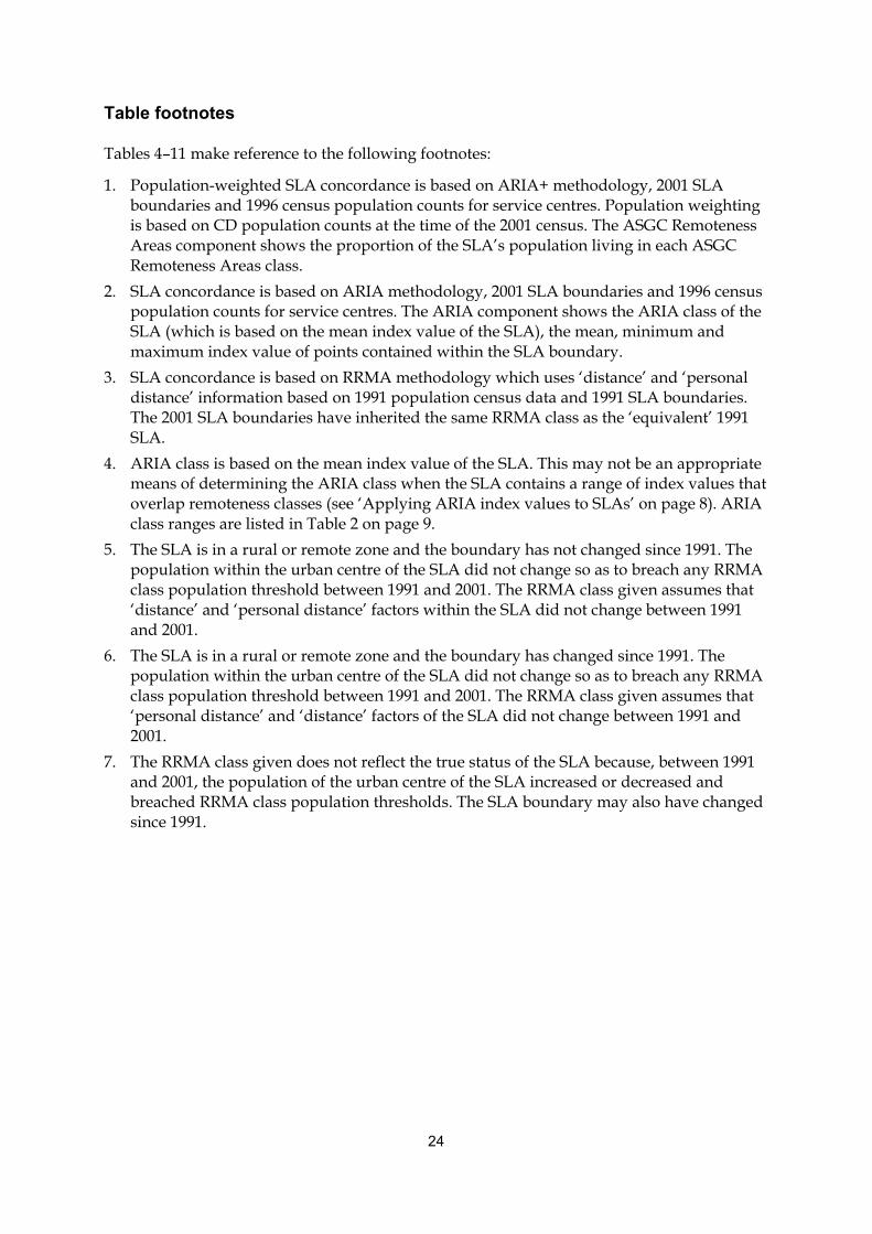
Table footnotes
Tables 4–11 make reference to the following footnotes:
1. Population-weighted SLA concordance is based on ARIA+ methodology, 2001 SLA boundaries and 1996 census population counts for service centres. Population weighting is based on CD population counts at the time of the 2001 census. The ASGC Remoteness Areas component shows the proportion of the SLA’s population living in each ASGC Remoteness Areas class.
2. SLA concordance is based on ARIA methodology, 2001 SLA boundaries and 1996 census population counts for service centres. The ARIA component shows the ARIA class of the SLA (which is based on the mean index value of the SLA), the mean, minimum and maximum index value of points contained within the SLA boundary.
3. SLA concordance is based on RRMA methodology which uses ‘distance’ and ‘personal distance’ information based on 1991 population census data and 1991 SLA boundaries. The 2001 SLA boundaries have inherited the same RRMA class as the ‘equivalent’ 1991 SLA.
4. ARIA class is based on the mean index value of the SLA. This may not be an appropriate means of determining the ARIA class when the SLA contains a range of index values that overlap remoteness classes (see ‘Applying ARIA index values to SLAs’ on page 8). ARIA class ranges are listed in Table 2 on page 9.
5. The SLA is in a rural or remote zone and the boundary has not changed since 1991. The population within the urban centre of the SLA did not change so as to breach any RRMA class population threshold between 1991 and 2001. The RRMA class given assumes that ‘distance’ and ‘personal distance’ factors within the SLA did not change between 1991 and 2001.
6. The SLA is in a rural or remote zone and the boundary has changed since 1991. The population within the urban centre of the SLA did not change so as to breach any RRMA class population threshold between 1991 and 2001. The RRMA class given assumes that ‘personal distance’ and ‘distance’ factors of the SLA did not change between 1991 and 2001.
7. The RRMA class given does not reflect the true status of the SLA because, between 1991 and 2001, the population of the urban centre of the SLA increased or decreased and breached RRMA class population thresholds. The SLA boundary may also have changed since 1991.

25
SLA suffixes Most of the SLAs in the following geographical guide (Tables 4–11) have a suffix indicating the SLA’s Local Government Area (LGA) status. The suffixes are: (A) New South Wales Area (B) Borough (C) City (CGC) Community Government Council (DC) District Council (M) Municipality (RC) Rural City (S) Shire (T) Town SLAs that do not have a suffix are localities or suburbs within a LGA. For example, Acacia Ridge is in the LGA of Brisbane City (ABS 2002).
Finding an SLA The geographical guide (Tables 4–11) is in the state/territory order as used in the Australian Standard Geographical Classification: • New South Wales (page 26) • Victoria (page 32) • Queensland (page 38) • South Australia (page 53) • Western Australia (page 57) • Tasmania (page 62) • Northern Territory (page 64) • Australian Capital Territory and Other Territories (page 67). SLAs are listed in SLA code order which, with the exception of Queensland and the Northern Territory, corresponds to alphabetical order according to SLA name. An alphabetical guide has been included with the Queensland table (Table 6) and Northern Territory table (Table 10) to assist in locating SLAs within these jurisdictions.
26
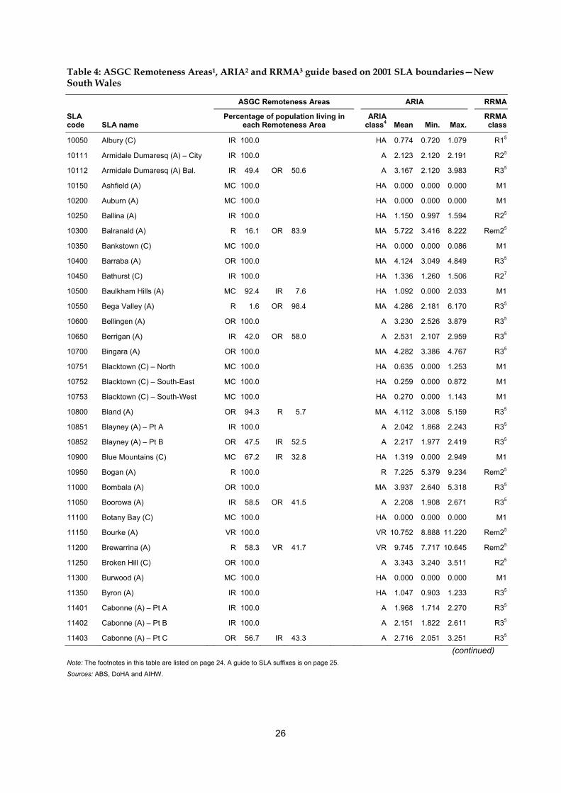
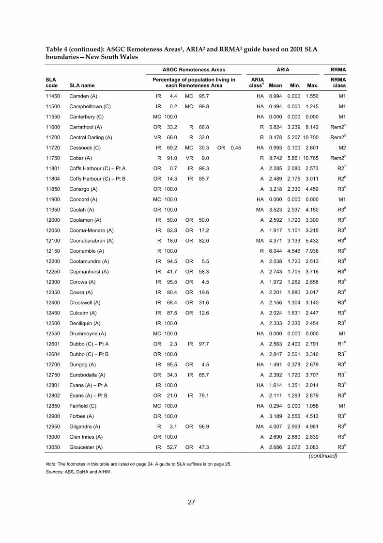
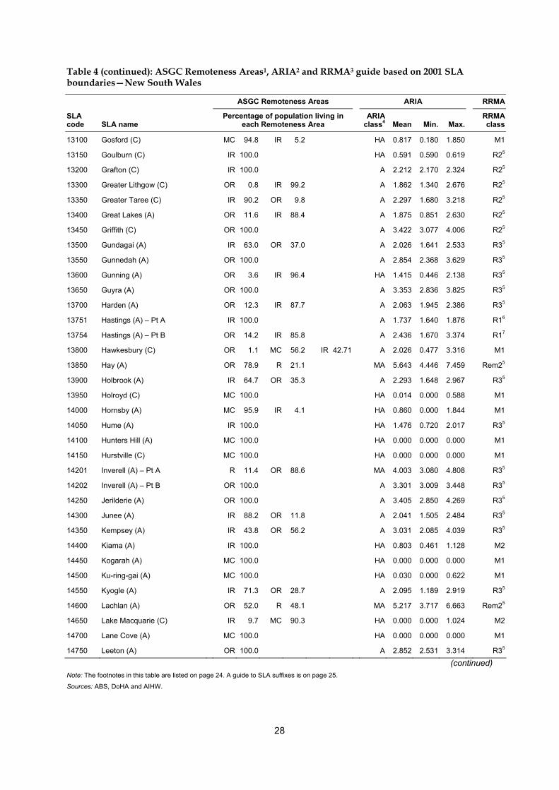
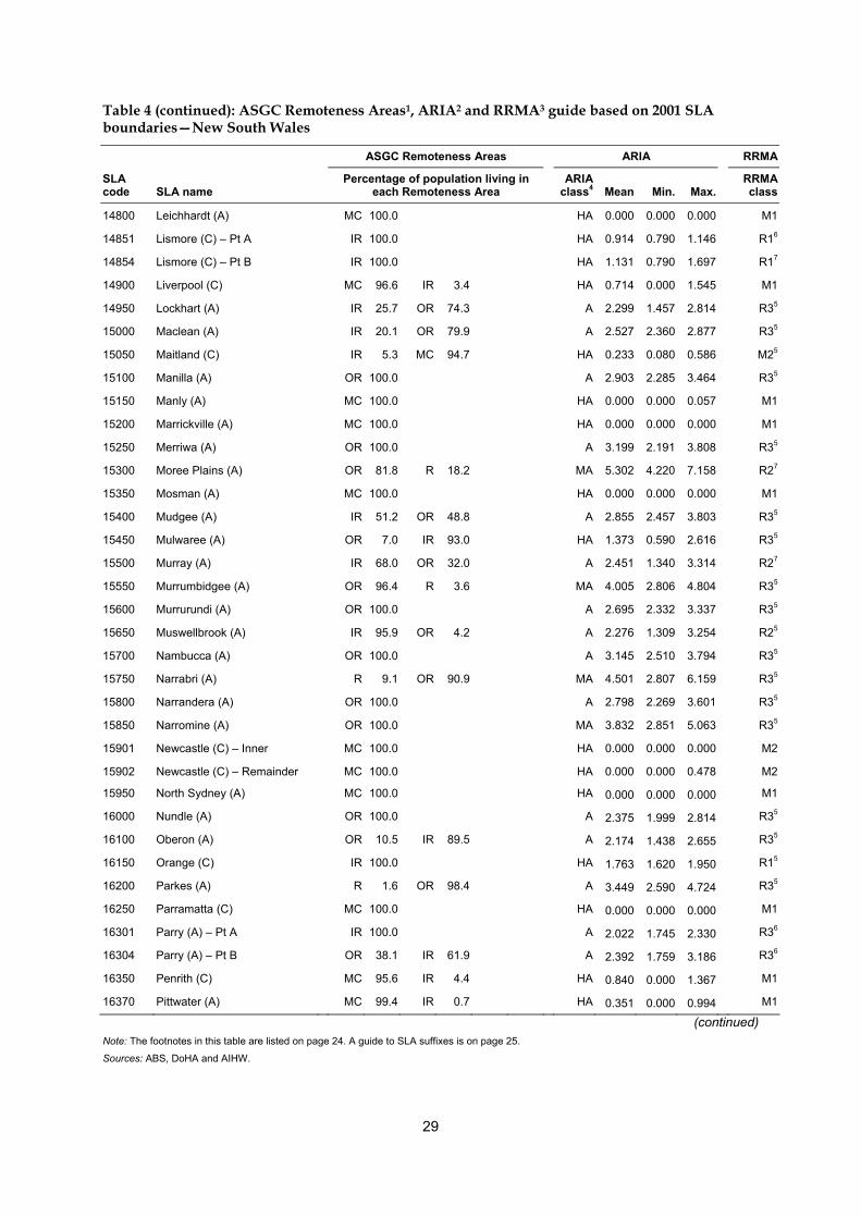
Table 4: ASGC Remoteness Areas1, ARIA2 and RRMA3 guide based on 2001 SLA boundaries—New South Wales
ASGC Remoteness Areas ARIA RRMA
SLA code SLA name
Percentage of population living in each Remoteness Area
ARIA class4
Mean
Min. Max.
RRMA class
10050 Albury (C) IR 100.0 HA 0.774 0.720 1.079 R15
10111 Armidale Dumaresq (A) – City IR 100.0 A 2.123 2.120 2.191 R25
10112 Armidale Dumaresq (A) Bal. IR 49.4 OR 50.6 A 3.167 2.120 3.983 R35
10150 Ashfield (A) MC 100.0 HA 0.000 0.000 0.000 M1
10200 Auburn (A) MC 100.0 HA 0.000 0.000 0.000 M1
10250 Ballina (A) IR 100.0 HA 1.150 0.997 1.594 R25
10300 Balranald (A) R 16.1 OR 83.9 MA 5.722 3.416 8.222 Rem25
10350 Bankstown (C) MC 100.0 HA 0.000 0.000 0.086 M1
10400 Barraba (A) OR 100.0 MA 4.124 3.049 4.849 R35
10450 Bathurst (C) IR 100.0 HA 1.336 1.260 1.506 R27
10500 Baulkham Hills (A) MC 92.4 IR 7.6 HA 1.092 0.000 2.033 M1
10550 Bega Valley (A) R 1.6 OR 98.4 MA 4.286 2.181 6.170 R35
10600 Bellingen (A) OR 100.0 A 3.230 2.526 3.879 R35
10650 Berrigan (A) IR 42.0 OR 58.0 A 2.531 2.107 2.959 R35
10700 Bingara (A) OR 100.0 MA 4.282 3.386 4.767 R35
10751 Blacktown (C) – North MC 100.0 HA 0.635 0.000 1.253 M1
10752 Blacktown (C) – South-East MC 100.0 HA 0.259 0.000 0.872 M1
10753 Blacktown (C) – South-West MC 100.0 HA 0.270 0.000 1.143 M1
10800 Bland (A) OR 94.3 R 5.7 MA 4.112 3.008 5.159 R35
10851 Blayney (A) – Pt A IR 100.0 A 2.042 1.868 2.243 R35
10852 Blayney (A) – Pt B OR 47.5 IR 52.5 A 2.217 1.977 2.419 R35
10900 Blue Mountains (C) MC 67.2 IR 32.8 HA 1.319 0.000 2.949 M1
10950 Bogan (A) R 100.0 R 7.225 5.379 9.234 Rem25
11000 Bombala (A) OR 100.0 MA 3.937 2.640 5.318 R35
11050 Boorowa (A) IR 58.5 OR 41.5 A 2.208 1.908 2.671 R35
11100 Botany Bay (C) MC 100.0 HA 0.000 0.000 0.000 M1
11150 Bourke (A) VR 100.0 VR 10.752 8.888 11.220 Rem25
11200 Brewarrina (A) R 58.3 VR 41.7 VR 9.745 7.717 10.645 Rem25
11250 Broken Hill (C) OR 100.0 A 3.343 3.240 3.511 R25
11300 Burwood (A) MC 100.0 HA 0.000 0.000 0.000 M1
11350 Byron (A) IR 100.0 HA 1.047 0.903 1.233 R35
11401 Cabonne (A) – Pt A IR 100.0 A 1.968 1.714 2.270 R35
11402 Cabonne (A) – Pt B IR 100.0 A 2.151 1.822 2.611 R35
11403 Cabonne (A) – Pt C OR 56.7 IR 43.3 A 2.716 2.051 3.251 R35
(continued) Note: The footnotes in this table are listed on page 24. A guide to SLA suffixes is on page 25.
Sources: ABS, DoHA and AIHW.
27
Table 4 (continued): ASGC Remoteness Areas1, ARIA2 and RRMA3 guide based on 2001 SLA boundaries—New South Wales
ASGC Remoteness Areas ARIA RRMA
SLA code SLA name
Percentage of population living in each Remoteness Area
ARIA class4
Mean
Min. Max.
RRMA class
11450 Camden (A) IR 4.4 MC 95.7 HA 0.994 0.000 1.550 M1
11500 Campbelltown (C) IR 0.2 MC 99.8 HA 0.494 0.000 1.245 M1
11550 Canterbury (C) MC 100.0 HA 0.000 0.000 0.000 M1
11600 Carrathool (A) OR 33.2 R 66.8 R 5.824 3.239 8.142 Rem25
11700 Central Darling (A) VR 68.0 R 32.0 R 8.478 5.207 10.700 Rem25
11720 Cessnock (C) IR 69.2 MC 30.3 OR 0.45 HA 0.993 0.100 2.601 M2
11750 Cobar (A) R 91.0 VR 9.0 R 8.742 5.861 10.765 Rem25
11801 Coffs Harbour (C) – Pt A OR 0.7 IR 99.3 A 2.285 2.080 2.573 R27
11804 Coffs Harbour (C) – Pt B OR 14.3 IR 85.7 A 2.489 2.175 3.011 R26
11850 Conargo (A) OR 100.0 A 3.218 2.330 4.459 R35
11900 Concord (A) MC 100.0 HA 0.000 0.000 0.000 M1
11950 Coolah (A) OR 100.0 MA 3.523 2.937 4.150 R35
12000 Coolamon (A) IR 50.0 OR 50.0 A 2.592 1.720 3.300 R35
12050 Cooma-Monaro (A) IR 82.8 OR 17.2 A 1.917 1.101 3.215 R35
12100 Coonabarabran (A) R 18.0 OR 82.0 MA 4.371 3.133 5.432 R35
12150 Coonamble (A) R 100.0 R 6.044 4.546 7.938 R35
12200 Cootamundra (A) IR 94.5 OR 5.5 A 2.038 1.720 2.513 R35
12250 Copmanhurst (A) IR 41.7 OR 58.3 A 2.743 1.705 3.716 R35
12300 Corowa (A) IR 95.5 OR 4.5 A 1.972 1.262 2.858 R35
12350 Cowra (A) IR 80.4 OR 19.6 A 2.201 1.880 3.017 R35
12400 Crookwell (A) IR 68.4 OR 31.6 A 2.156 1.304 3.140 R35
12450 Culcairn (A) IR 87.5 OR 12.6 A 2.024 1.631 2.447 R35
12500 Deniliquin (A) IR 100.0 A 2.333 2.330 2.454 R35
12550 Drummoyne (A) MC 100.0 HA 0.000 0.000 0.000 M1
12601 Dubbo (C) – Pt A OR 2.3 IR 97.7 A 2.563 2.400 2.791 R16
12604 Dubbo (C) – Pt B OR 100.0 A 2.847 2.501 3.310 R37
12700 Dungog (A) IR 95.5 OR 4.5 HA 1.491 0.378 2.679 R35
12750 Eurobodalla (A) OR 34.3 IR 65.7 A 2.392 1.720 3.707 R37
12801 Evans (A) – Pt A IR 100.0 HA 1.614 1.351 2.014 R35
12802 Evans (A) – Pt B OR 21.0 IR 79.1 A 2.111 1.293 2.879 R35
12850 Fairfield (C) MC 100.0 HA 0.294 0.000 1.058 M1
12900 Forbes (A) OR 100.0 A 3.189 2.556 4.513 R35
12950 Gilgandra (A) R 3.1 OR 96.9 MA 4.007 2.993 4.961 R35
13000 Glen Innes (A) OR 100.0 A 2.690 2.680 2.839 R35
13050 Gloucester (A) IR 52.7 OR 47.3 A 2.686 2.072 3.083 R35
(continued) Note: The footnotes in this table are listed on page 24. A guide to SLA suffixes is on page 25.
Sources: ABS, DoHA and AIHW.
28
Table 4 (continued): ASGC Remoteness Areas1, ARIA2 and RRMA3 guide based on 2001 SLA boundaries—New South Wales
ASGC Remoteness Areas ARIA RRMA
SLA code SLA name
Percentage of population living in each Remoteness Area
ARIA class4
Mean
Min. Max.
RRMA class
13100 Gosford (C) MC 94.8 IR 5.2 HA 0.817 0.180 1.850 M1
13150 Goulburn (C) IR 100.0 HA 0.591 0.590 0.619 R25
13200 Grafton (C) IR 100.0 A 2.212 2.170 2.324 R25
13300 Greater Lithgow (C) OR 0.8 IR 99.2 A 1.862 1.340 2.676 R25
13350 Greater Taree (C) IR 90.2 OR 9.8 A 2.297 1.680 3.218 R25
13400 Great Lakes (A) OR 11.6 IR 88.4 A 1.875 0.851 2.630 R25
13450 Griffith (C) OR 100.0 A 3.422 3.077 4.006 R25
13500 Gundagai (A) IR 63.0 OR 37.0 A 2.026 1.641 2.533 R35
13550 Gunnedah (A) OR 100.0 A 2.854 2.368 3.629 R35
13600 Gunning (A) OR 3.6 IR 96.4 HA 1.415 0.446 2.138 R35
13650 Guyra (A) OR 100.0 A 3.353 2.836 3.825 R35
13700 Harden (A) OR 12.3 IR 87.7 A 2.063 1.945 2.386 R35
13751 Hastings (A) – Pt A IR 100.0 A 1.737 1.640 1.876 R16
13754 Hastings (A) – Pt B OR 14.2 IR 85.8 A 2.436 1.670 3.374 R17
13800 Hawkesbury (C) OR 1.1 MC 56.2 IR 42.71 A 2.026 0.477 3.316 M1
13850 Hay (A) OR 78.9 R 21.1 MA 5.643 4.446 7.459 Rem25
13900 Holbrook (A) IR 64.7 OR 35.3 A 2.293 1.648 2.967 R35
13950 Holroyd (C) MC 100.0 HA 0.014 0.000 0.588 M1
14000 Hornsby (A) MC 95.9 IR 4.1 HA 0.860 0.000 1.844 M1
14050 Hume (A) IR 100.0 HA 1.476 0.720 2.017 R35
14100 Hunters Hill (A) MC 100.0 HA 0.000 0.000 0.000 M1
14150 Hurstville (C) MC 100.0 HA 0.000 0.000 0.000 M1
14201 Inverell (A) – Pt A R 11.4 OR 88.6 MA 4.003 3.080 4.808 R35
14202 Inverell (A) – Pt B OR 100.0 A 3.301 3.009 3.448 R35
14250 Jerilderie (A) OR 100.0 A 3.405 2.850 4.269 R35
14300 Junee (A) IR 88.2 OR 11.8 A 2.041 1.505 2.484 R35
14350 Kempsey (A) IR 43.8 OR 56.2 A 3.031 2.085 4.039 R35
14400 Kiama (A) IR 100.0 HA 0.803 0.461 1.128 M2
14450 Kogarah (A) MC 100.0 HA 0.000 0.000 0.000 M1
14500 Ku-ring-gai (A) MC 100.0 HA 0.030 0.000 0.622 M1
14550 Kyogle (A) IR 71.3 OR 28.7 A 2.095 1.189 2.919 R35
14600 Lachlan (A) OR 52.0 R 48.1 MA 5.217 3.717 6.663 Rem25
14650 Lake Macquarie (C) IR 9.7 MC 90.3 HA 0.000 0.000 1.024 M2
14700 Lane Cove (A) MC 100.0 HA 0.000 0.000 0.000 M1
14750 Leeton (A) OR 100.0 A 2.852 2.531 3.314 R35
(continued) Note: The footnotes in this table are listed on page 24. A guide to SLA suffixes is on page 25.
Sources: ABS, DoHA and AIHW.
29
Table 4 (continued): ASGC Remoteness Areas1, ARIA2 and RRMA3 guide based on 2001 SLA boundaries—New South Wales
ASGC Remoteness Areas ARIA RRMA
SLA code SLA name
Percentage of population living in each Remoteness Area
ARIA class4
Mean
Min. Max.
RRMA class
14800 Leichhardt (A) MC 100.0 HA 0.000 0.000 0.000 M1
14851 Lismore (C) – Pt A IR 100.0 HA 0.914 0.790 1.146 R16
14854 Lismore (C) – Pt B IR 100.0 HA 1.131 0.790 1.697 R17
14900 Liverpool (C) MC 96.6 IR 3.4 HA 0.714 0.000 1.545 M1
14950 Lockhart (A) IR 25.7 OR 74.3 A 2.299 1.457 2.814 R35
15000 Maclean (A) IR 20.1 OR 79.9 A 2.527 2.360 2.877 R35
15050 Maitland (C) IR 5.3 MC 94.7 HA 0.233 0.080 0.586 M25
15100 Manilla (A) OR 100.0 A 2.903 2.285 3.464 R35
15150 Manly (A) MC 100.0 HA 0.000 0.000 0.057 M1
15200 Marrickville (A) MC 100.0 HA 0.000 0.000 0.000 M1
15250 Merriwa (A) OR 100.0 A 3.199 2.191 3.808 R35
15300 Moree Plains (A) OR 81.8 R 18.2 MA 5.302 4.220 7.158 R27
15350 Mosman (A) MC 100.0 HA 0.000 0.000 0.000 M1
15400 Mudgee (A) IR 51.2 OR 48.8 A 2.855 2.457 3.803 R35
15450 Mulwaree (A) OR 7.0 IR 93.0 HA 1.373 0.590 2.616 R35
15500 Murray (A) IR 68.0 OR 32.0 A 2.451 1.340 3.314 R27
15550 Murrumbidgee (A) OR 96.4 R 3.6 MA 4.005 2.806 4.804 R35
15600 Murrurundi (A) OR 100.0 A 2.695 2.332 3.337 R35
15650 Muswellbrook (A) IR 95.9 OR 4.2 A 2.276 1.309 3.254 R25
15700 Nambucca (A) OR 100.0 A 3.145 2.510 3.794 R35
15750 Narrabri (A) R 9.1 OR 90.9 MA 4.501 2.807 6.159 R35
15800 Narrandera (A) OR 100.0 A 2.798 2.269 3.601 R35
15850 Narromine (A) OR 100.0 MA 3.832 2.851 5.063 R35
15901 Newcastle (C) – Inner MC 100.0 HA 0.000 0.000 0.000 M2
15902 Newcastle (C) – Remainder MC 100.0 HA 0.000 0.000 0.478 M2
15950 North Sydney (A) MC 100.0 HA 0.000 0.000 0.000 M1
16000 Nundle (A) OR 100.0 A 2.375 1.999 2.814 R35
16100 Oberon (A) OR 10.5 IR 89.5 A 2.174 1.438 2.655 R35
16150 Orange (C) IR 100.0 HA 1.763 1.620 1.950 R15
16200 Parkes (A) R 1.6 OR 98.4 A 3.449 2.590 4.724 R35
16250 Parramatta (C) MC 100.0 HA 0.000 0.000 0.000 M1
16301 Parry (A) – Pt A IR 100.0 A 2.022 1.745 2.330 R36
16304 Parry (A) – Pt B OR 38.1 IR 61.9 A 2.392 1.759 3.186 R36
16350 Penrith (C) MC 95.6 IR 4.4 HA 0.840 0.000 1.367 M1
16370 Pittwater (A) MC 99.4 IR 0.7 HA 0.351 0.000 0.994 M1
(continued) Note: The footnotes in this table are listed on page 24. A guide to SLA suffixes is on page 25.
Sources: ABS, DoHA and AIHW.

30
Table 4 (continued): ASGC Remoteness Areas1, ARIA2 and RRMA3 guide based on 2001 SLA boundaries—New South Wales
ASGC Remoteness Areas ARIA RRMA
SLA code SLA name
Percentage of population living in each Remoteness Area
ARIA class4
Mean
Min. Max.
RRMA class
16400 Port Stephens (A) MC 24.4 IR 75.6 HA 0.589 0.000 1.025 M2
16421 Pristine Waters (A) – Nymboida IR 25.7 OR 74.3 A 3.197 2.211 3.959 R35
16422 Pristine Waters (A) – Ulmarra IR 11.4 OR 88.6 A 2.519 2.198 2.907 R35
16450 Queanbeyan (C) MC 100.0 HA 0.092 0.040 0.128 M2
16500 Quirindi (A) OR 100.0 A 2.870 2.130 3.726 R35
16550 Randwick (C) MC 100.0 HA 0.000 0.000 0.000 M1
16611 Richmond Valley (A) – Casino IR 100.0 HA 1.188 1.131 1.348 R27
16612 Richmond Valley (A) Bal. OR 3.4 IR 96.6 HA 1.713 1.050 2.539 R35
16650 Rockdale (C) MC 100.0 HA 0.000 0.000 0.000 M1
16700 Ryde (C) MC 100.0 HA 0.000 0.000 0.000 M1
16750 Rylstone (A) IR 39.9 OR 60.2 A 2.793 2.104 3.199 R35
16800 Scone (A) IR 72.9 OR 27.1 A 2.441 1.640 3.042 R35
16850 Severn (A) OR 100.0 A 3.249 2.680 4.008 R35
16900 Shellharbour (C) IR 1.4 MC 98.6 HA 0.498 0.190 0.939 M2
16951 Shoalhaven (C) – Pt A IR 100.0 HA 0.790 0.670 0.961 R26
16952 Shoalhaven (C) – Pt B IR 98.2 OR 1.8 HA 1.545 0.781 2.355 R27
17000 Singleton (A) OR 1.1 IR 98.9 HA 1.683 0.423 3.118 R25
17050 Snowy River (A) IR 8.4 OR 91.6 A 2.847 1.529 5.225 R35
17070 South Sydney (C) MC 100.0 HA 0.000 0.000 0.000 M1
17100 Strathfield (A) MC 100.0 HA 0.000 0.000 0.000 M1
17151 Sutherland Shire (A) – East IR 2.8 MC 97.2 HA 0.601 0.000 1.250 M1
17152 Sutherland Shire (A) – West IR 0.4 MC 99.6 HA 0.302 0.000 0.936 M1
17201 Sydney (C) – Inner MC 100.0 HA 0.000 0.000 0.000 M1
17202 Sydney (C) – Remainder MC 100.0 HA 0.000 0.000 0.000 M1
17250 Tallaganda (A) IR 5.9 OR 94.1 HA 1.719 1.021 2.331 R35
17300 Tamworth (C) IR 100.0 HA 1.783 1.710 2.020 R15
17350 Temora (A) OR 100.0 A 2.808 2.154 3.671 R35
17400 Tenterfield (A) OR 100.0 A 3.274 2.032 4.690 R35
17450 Tumbarumba (A) OR 100.0 A 3.040 2.180 4.618 R35
17500 Tumut (A) IR 90.8 OR 9.2 A 1.917 1.351 2.959 R35
17551 Tweed (A) – Pt A IR 2.7 MC 97.3 HA 0.335 0.044 0.539 M2
17552 Tweed (A) – Pt B MC 11.3 IR 88.7 HA 0.853 0.401 1.447 R35
17650 Uralla (A) IR 40.2 OR 59.8 A 2.958 2.254 3.736 R35
17700 Urana (A) OR 100.0 A 2.820 2.026 3.622 R35
17751 Wagga Wagga (C) – Pt A IR 100.0 HA 1.201 1.070 1.367 R16
(continued) Note: The footnotes in this table are listed on page 24. A guide to SLA suffixes is on page 25.
Sources: ABS, DoHA and AIHW.
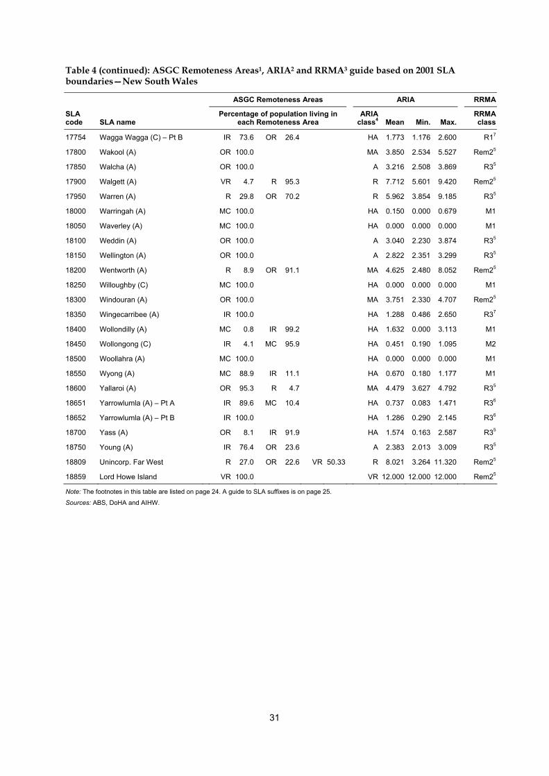
31
Table 4 (continued): ASGC Remoteness Areas1, ARIA2 and RRMA3 guide based on 2001 SLA boundaries—New South Wales
ASGC Remoteness Areas ARIA RRMA
SLA code SLA name
Percentage of population living in each Remoteness Area
ARIA class4
Mean
Min. Max.
RRMA class
17754 Wagga Wagga (C) – Pt B IR 73.6 OR 26.4 HA 1.773 1.176 2.600 R17
17800 Wakool (A) OR 100.0 MA 3.850 2.534 5.527 Rem25
17850 Walcha (A) OR 100.0 A 3.216 2.508 3.869 R35
17900 Walgett (A) VR 4.7 R 95.3 R 7.712 5.601 9.420 Rem25
17950 Warren (A) R 29.8 OR 70.2 R 5.962 3.854 9.185 R35
18000 Warringah (A) MC 100.0 HA 0.150 0.000 0.679 M1
18050 Waverley (A) MC 100.0 HA 0.000 0.000 0.000 M1
18100 Weddin (A) OR 100.0 A 3.040 2.230 3.874 R35
18150 Wellington (A) OR 100.0 A 2.822 2.351 3.299 R35
18200 Wentworth (A) R 8.9 OR 91.1 MA 4.625 2.480 8.052 Rem25
18250 Willoughby (C) MC 100.0 HA 0.000 0.000 0.000 M1
18300 Windouran (A) OR 100.0 MA 3.751 2.330 4.707 Rem25
18350 Wingecarribee (A) IR 100.0 HA 1.288 0.486 2.650 R37
18400 Wollondilly (A) MC 0.8 IR 99.2 HA 1.632 0.000 3.113 M1
18450 Wollongong (C) IR 4.1 MC 95.9 HA 0.451 0.190 1.095 M2
18500 Woollahra (A) MC 100.0 HA 0.000 0.000 0.000 M1
18550 Wyong (A) MC 88.9 IR 11.1 HA 0.670 0.180 1.177 M1
18600 Yallaroi (A) OR 95.3 R 4.7 MA 4.479 3.627 4.792 R35
18651 Yarrowlumla (A) – Pt A IR 89.6 MC 10.4 HA 0.737 0.083 1.471 R36
18652 Yarrowlumla (A) – Pt B IR 100.0 HA 1.286 0.290 2.145 R36
18700 Yass (A) OR 8.1 IR 91.9 HA 1.574 0.163 2.587 R35
18750 Young (A) IR 76.4 OR 23.6 A 2.383 2.013 3.009 R35
18809 Unincorp. Far West R 27.0 OR 22.6 VR 50.33 R 8.021 3.264 11.320 Rem25
18859 Lord Howe Island VR 100.0 VR 12.000 12.000 12.000 Rem25
Note: The footnotes in this table are listed on page 24. A guide to SLA suffixes is on page 25.
Sources: ABS, DoHA and AIHW.
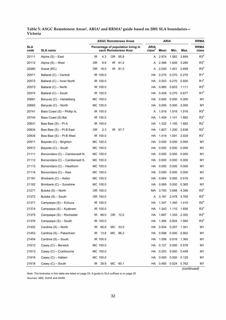
32
Table 5: ASGC Remoteness Areas1, ARIA2 and RRMA3 guide based on 2001 SLA boundaries—Victoria
ASGC Remoteness Areas ARIA RRMA
SLA code SLA name
Percentage of population living in each Remoteness Area
ARIA class4
Mean
Min. Max.
RRMA class
20111 Alpine (S) – East IR 4.3 OR 95.8 A 2.974 1.582 3.849 R36
20112 Alpine (S) – West OR 8.8 IR 91.2 A 2.366 1.626 3.280 R36
20260 Ararat (RC) OR 19.0 IR 81.0 A 2.020 1.451 2.659 R36
20571 Ballarat (C) – Central IR 100.0 HA 0.270 0.270 0.270 R16
20572 Ballarat (C) – Inner North IR 100.0 HA 0.553 0.270 0.920 R16
20573 Ballarat (C) – North IR 100.0 HA 0.885 0.653 1.111 R36
20574 Ballarat (C) – South IR 100.0 HA 0.459 0.270 0.677 R16
20661 Banyule (C) – Heidelberg MC 100.0 HA 0.000 0.000 0.000 M1
20662 Banyule (C) – North MC 100.0 HA 0.000 0.000 0.000 M1
20741 Bass Coast (S) – Phillip Is. IR 100.0 A 1.918 1.918 1.918 R35
20744 Bass Coast (S) Bal IR 100.0 HA 1.459 1.141 1.882 R36
20831 Baw Baw (S) – Pt A IR 100.0 HA 1.322 1.100 1.682 R27
20834 Baw Baw (S) – Pt B East OR 2.3 IR 97.7 HA 1.827 1.200 2.638 R27
20835 Baw Baw (S) – Pt B West IR 100.0 HA 1.419 1.091 2.029 R37
20911 Bayside (C) – Brighton MC 100.0 HA 0.000 0.000 0.000 M1
20912 Bayside (C) – South MC 100.0 HA 0.000 0.000 0.000 M1
21111 Boroondara (C) – Camberwell N. MC 100.0 HA 0.000 0.000 0.000 M1
21112 Boroondara (C) – Camberwell S. MC 100.0 HA 0.000 0.000 0.000 M1
21113 Boroondara (C) – Hawthorn MC 100.0 HA 0.000 0.000 0.000 M1
21114 Boroondara (C) – Kew MC 100.0 HA 0.000 0.000 0.000 M1
21181 Brimbank (C) – Keilor MC 100.0 HA 0.064 0.000 0.516 M1
21182 Brimbank (C) – Sunshine MC 100.0 HA 0.069 0.000 0.365 M1
21271 Buloke (S) – North OR 100.0 MA 3.793 3.066 4.356 R36
21272 Buloke (S) – South OR 100.0 A 3.181 2.478 3.765 R36
21371 Campaspe (S) – Echuca IR 100.0 HA 1.347 1.340 1.416 R26
21374 Campaspe (S) – Kyabram IR 100.0 HA 1.343 1.110 1.656 R36
21375 Campaspe (S) – Rochester IR 88.0 OR 12.0 HA 1.687 1.335 2.352 R36
21376 Campaspe (S) – South IR 100.0 HA 1.384 0.904 1.560 R36
21452 Cardinia (S) – North IR 66.6 MC 33.5 HA 0.934 0.207 1.301 M1
21453 Cardinia (S) – Pakenham IR 13.8 MC 86.2 HA 0.598 0.000 0.902 M1
21454 Cardinia (S) – South IR 100.0 HA 1.056 0.616 1.360 M1
21612 Casey (C) – Berwick MC 100.0 HA 0.127 0.000 0.578 M1
21613 Casey (C) – Cranbourne MC 100.0 HA 0.253 0.000 0.448 M1
21616 Casey (C) – Hallam MC 100.0 HA 0.000 0.000 0.129 M1
21618 Casey (C) – South IR 39.9 MC 60.1 HA 0.485 0.024 0.762 M1
(continued) Note: The footnotes in this table are listed on page 24. A guide to SLA suffixes is on page 25.
Sources: ABS, DoHA and AIHW.
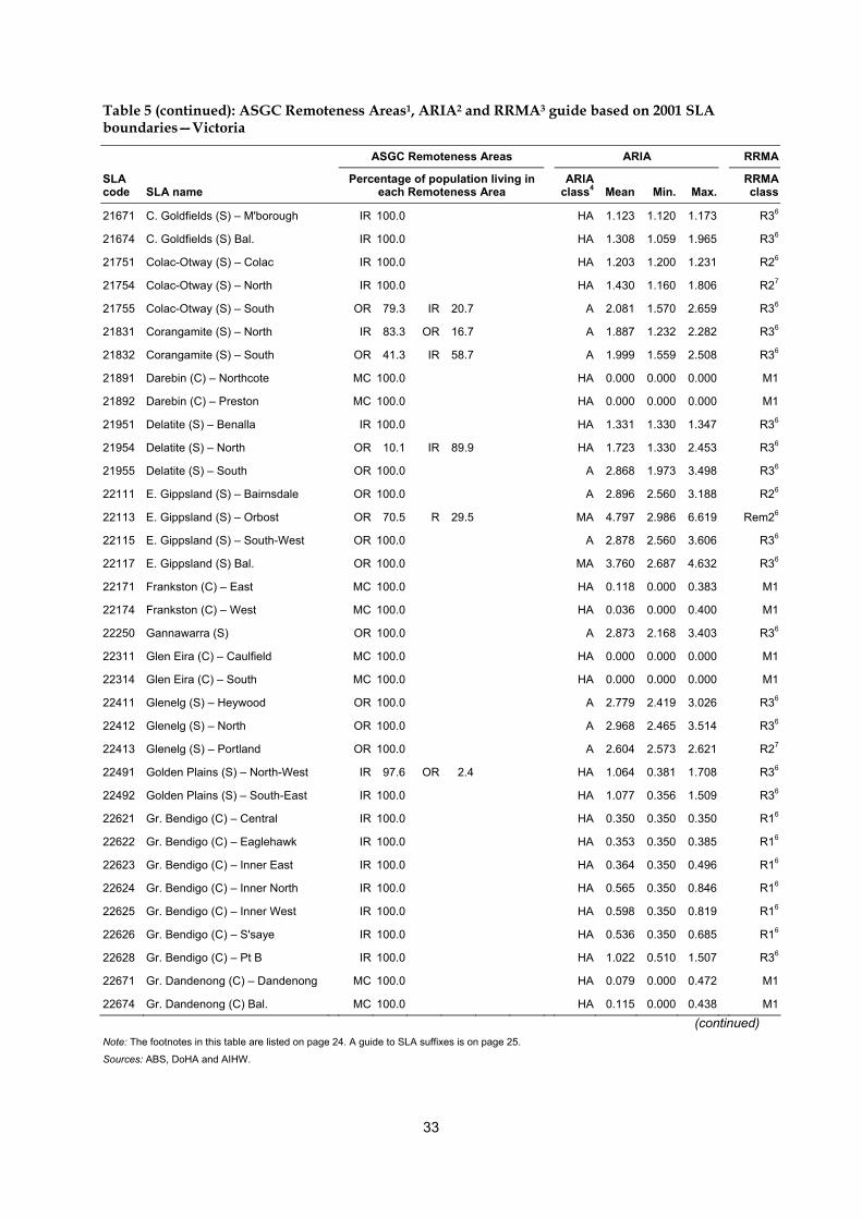
33
Table 5 (continued): ASGC Remoteness Areas1, ARIA2 and RRMA3 guide based on 2001 SLA boundaries—Victoria
ASGC Remoteness Areas ARIA RRMA
SLA code SLA name
Percentage of population living in each Remoteness Area
ARIA class4
Mean
Min. Max.
RRMA class
21671 C. Goldfields (S) – M'borough IR 100.0 HA 1.123 1.120 1.173 R36
21674 C. Goldfields (S) Bal. IR 100.0 HA 1.308 1.059 1.965 R36
21751 Colac-Otway (S) – Colac IR 100.0 HA 1.203 1.200 1.231 R26
21754 Colac-Otway (S) – North IR 100.0 HA 1.430 1.160 1.806 R27
21755 Colac-Otway (S) – South OR 79.3 IR 20.7 A 2.081 1.570 2.659 R36
21831 Corangamite (S) – North IR 83.3 OR 16.7 A 1.887 1.232 2.282 R36
21832 Corangamite (S) – South OR 41.3 IR 58.7 A 1.999 1.559 2.508 R36
21891 Darebin (C) – Northcote MC 100.0 HA 0.000 0.000 0.000 M1
21892 Darebin (C) – Preston MC 100.0 HA 0.000 0.000 0.000 M1
21951 Delatite (S) – Benalla IR 100.0 HA 1.331 1.330 1.347 R36
21954 Delatite (S) – North OR 10.1 IR 89.9 HA 1.723 1.330 2.453 R36
21955 Delatite (S) – South OR 100.0 A 2.868 1.973 3.498 R36
22111 E. Gippsland (S) – Bairnsdale OR 100.0 A 2.896 2.560 3.188 R26
22113 E. Gippsland (S) – Orbost OR 70.5 R 29.5 MA 4.797 2.986 6.619 Rem26
22115 E. Gippsland (S) – South-West OR 100.0 A 2.878 2.560 3.606 R36
22117 E. Gippsland (S) Bal. OR 100.0 MA 3.760 2.687 4.632 R36
22171 Frankston (C) – East MC 100.0 HA 0.118 0.000 0.383 M1
22174 Frankston (C) – West MC 100.0 HA 0.036 0.000 0.400 M1
22250 Gannawarra (S) OR 100.0 A 2.873 2.168 3.403 R36
22311 Glen Eira (C) – Caulfield MC 100.0 HA 0.000 0.000 0.000 M1
22314 Glen Eira (C) – South MC 100.0 HA 0.000 0.000 0.000 M1
22411 Glenelg (S) – Heywood OR 100.0 A 2.779 2.419 3.026 R36
22412 Glenelg (S) – North OR 100.0 A 2.968 2.465 3.514 R36
22413 Glenelg (S) – Portland OR 100.0 A 2.604 2.573 2.621 R27
22491 Golden Plains (S) – North-West IR 97.6 OR 2.4 HA 1.064 0.381 1.708 R36
22492 Golden Plains (S) – South-East IR 100.0 HA 1.077 0.356 1.509 R36
22621 Gr. Bendigo (C) – Central IR 100.0 HA 0.350 0.350 0.350 R16
22622 Gr. Bendigo (C) – Eaglehawk IR 100.0 HA 0.353 0.350 0.385 R16
22623 Gr. Bendigo (C) – Inner East IR 100.0 HA 0.364 0.350 0.496 R16
22624 Gr. Bendigo (C) – Inner North IR 100.0 HA 0.565 0.350 0.846 R16
22625 Gr. Bendigo (C) – Inner West IR 100.0 HA 0.598 0.350 0.819 R16
22626 Gr. Bendigo (C) – S'saye IR 100.0 HA 0.536 0.350 0.685 R16
22628 Gr. Bendigo (C) – Pt B IR 100.0 HA 1.022 0.510 1.507 R36
22671 Gr. Dandenong (C) – Dandenong MC 100.0 HA 0.079 0.000 0.472 M1
22674 Gr. Dandenong (C) Bal. MC 100.0 HA 0.115 0.000 0.438 M1
(continued) Note: The footnotes in this table are listed on page 24. A guide to SLA suffixes is on page 25.
Sources: ABS, DoHA and AIHW.

34
Table 5 (continued): ASGC Remoteness Areas1, ARIA2 and RRMA3 guide based on 2001 SLA boundaries—Victoria
ASGC Remoteness Areas ARIA RRMA
SLA code SLA name
Percentage of population living in each Remoteness Area
ARIA class4
Mean
Min. Max.
RRMA class
Greater Geelong
22751 Bellarine – Inner IR 2.9 MC 97.1 HA 0.301 0.180 0.414 M25
22752 Corio – Inner MC 98.5 IR 1.5 HA 0.337 0.180 0.605 M25
22753 Geelong MC 100.0 HA 0.181 0.180 0.187 M25
22754 Geelong West MC 100.0 HA 0.180 0.180 0.180 M25
22755 Newtown MC 100.0 HA 0.180 0.180 0.180 M25
22756 South Barwon – Inner IR 5.0 MC 95.1 HA 0.312 0.180 0.511 M25
Alphabetical listing continued
22757 Greater Geelong (C) – Pt B IR 100.0 HA 0.562 0.380 0.789 R26
22758 Greater Geelong (C) – Pt C IR 100.0 HA 0.631 0.310 1.029 R36
22831 Gr. Shepparton (C) – Pt A IR 100.0 HA 1.109 0.930 1.307 R16
22834 Gr. Shepparton (C) – Pt B East IR 100.0 HA 1.404 1.050 1.701 R36
22835 Gr. Shepparton (C) – Pt B West
IR 100.0 HA 1.262 1.076 1.522 R36
22911 Hepburn (S) – East IR 100.0 HA 1.169 0.927 1.347 R36
22912 Hepburn (S) – West IR 100.0 HA 0.996 0.608 1.194 R36
22980 Hindmarsh (S) OR 87.3 R 12.7 MA 4.678 3.441 5.390 R36
23111 Hobsons Bay (C) – Altona MC 100.0 HA 0.057 0.000 0.346 M1
23112 Hobsons Bay (C) – Williamstown
MC 100.0 HA 0.000 0.000 0.000 M1
23191 Horsham (RC) – Central OR 100.0 A 2.836 2.830 2.917 R37
23194 Horsham (RC) Bal. OR 100.0 A 3.227 2.620 3.806 R37
23271 Hume (C) – Broadmeadows MC 100.0 HA 0.051 0.000 0.323 M1
23274 Hume (C) – Craigieburn IR 3.5 MC 96.5 HA 0.422 0.000 0.610 M1
23275 Hume (C) – Sunbury IR 7.7 MC 92.3 HA 0.663 0.297 0.922 M1
23351 Indigo (S) – Pt A IR 100.0 HA 1.367 1.010 1.858 R36
23352 Indigo (S) – Pt B IR 100.0 HA 1.354 1.231 1.818 R36
23431 Kingston (C) – North MC 100.0 HA 0.000 0.000 0.000 M1
23434 Kingston (C) – South MC 100.0 HA 0.000 0.000 0.000 M1
23671 Knox (C) – North MC 100.0 HA 0.000 0.000 0.000 M1
23674 Knox (C) – South MC 100.0 HA 0.013 0.000 0.227 M1
23811 Latrobe (C) – Moe IR 100.0 HA 1.167 1.100 1.245 R26
23814 Latrobe (C) – Morwell IR 100.0 HA 1.267 1.080 1.568 R25
23815 Latrobe (C) – Traralgon IR 100.0 HA 1.316 1.070 1.835 R25
23818 Latrobe (C) Bal. IR 100.0 HA 1.570 1.222 1.990 R36
23943 Loddon (S) – North IR 13.1 OR 86.9 A 2.238 1.132 3.013 R36
(continued) Note: The footnotes in this table are listed on page 24. A guide to SLA suffixes is on page 25.
Sources: ABS, DoHA and AIHW.
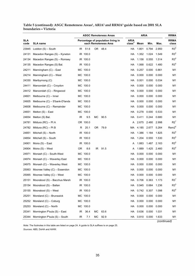
35
Table 5 (continued): ASGC Remoteness Areas1, ARIA2 and RRMA3 guide based on 2001 SLA boundaries—Victoria
ASGC Remoteness Areas ARIA RRMA
SLA code SLA name
Percentage of population living in each Remoteness Area
ARIA class4
Mean
Min. Max.
RRMA class
23945 Loddon (S) – South IR 51.6 OR 48.4 HA 1.801 0.794 2.950 R36
24131 Macedon Ranges (S) – Kyneton IR 100.0 HA 1.352 1.024 1.549 R36
24134 Macedon Ranges (S) – Romsey IR 100.0 HA 1.158 0.555 1.514 R36
24135 Macedon Ranges (S) Bal. IR 100.0 HA 1.068 0.622 1.480 R36
24211 Manningham (C) – East MC 100.0 HA 0.257 0.000 0.861 M1
24214 Manningham (C) – West MC 100.0 HA 0.000 0.000 0.000 M1
24330 Maribyrnong (C) MC 100.0 HA 0.001 0.000 0.034 M1
24411 Maroondah (C) – Croydon MC 100.0 HA 0.000 0.000 0.000 M1
24412 Maroondah (C) – Ringwood MC 100.0 HA 0.000 0.000 0.000 M1
24601 Melbourne (C) – Inner MC 100.0 HA 0.000 0.000 0.000 M1
24605 Melbourne (C) – S'bank-D'lands MC 100.0 HA 0.000 0.000 0.000 M1
24608 Melbourne (C) – Remainder MC 100.0 HA 0.000 0.000 0.000 M1
24651 Melton (S) – East MC 100.0 HA 0.278 0.000 0.533 M1
24654 Melton (S) Bal. IR 9.5 MC 90.5 HA 0.411 0.244 0.680 M1
24781 Mildura (RC) – Pt A OR 100.0 A 2.675 2.480 2.998 R27
24782 Mildura (RC) – Pt B R 20.1 OR 79.9 MA 4.185 2.677 5.264 Rem26
24851 Mitchell (S) – North IR 100.0 HA 1.386 1.184 1.825 R36
24854 Mitchell (S) – South IR 100.0 HA 1.204 0.555 1.530 R36
24901 Moira (S) – East IR 100.0 A 1.883 1.487 2.163 R36
24904 Moira (S) – West OR 8.6 IR 91.5 A 1.889 1.425 2.460 R36
24971 Monash (C) – South-West MC 100.0 HA 0.000 0.000 0.000 M1
24974 Monash (C) – Waverley East MC 100.0 HA 0.000 0.000 0.000 M1
24975 Monash (C) – Waverley West MC 100.0 HA 0.000 0.000 0.000 M1
25063 Moonee Valley (C) – Essendon MC 100.0 HA 0.000 0.000 0.000 M1
25065 Moonee Valley (C) – West MC 100.0 HA 0.000 0.000 0.000 M1
25151 Moorabool (S) – Bacchus Marsh IR 100.0 HA 0.706 0.363 1.173 R37
25154 Moorabool (S) – Ballan IR 100.0 HA 0.945 0.684 1.236 R35
25155 Moorabool (S) – West IR 100.0 HA 0.742 0.307 1.098 R36
25251 Moreland (C) – Brunswick MC 100.0 HA 0.000 0.000 0.000 M1
25252 Moreland (C) – Coburg MC 100.0 HA 0.000 0.000 0.000 M1
25253 Moreland (C) – North MC 100.0 HA 0.000 0.000 0.000 M1
25341 Mornington P'sula (S) – East IR 36.4 MC 63.6 HA 0.636 0.000 1.031 M1
25344 Mornington P'sula (S) – South IR 7.1 MC 92.9 HA 0.810 0.000 1.633 M1
(continued) Note: The footnotes in this table are listed on page 24. A guide to SLA suffixes is on page 25.
Sources: ABS, DoHA and AIHW.
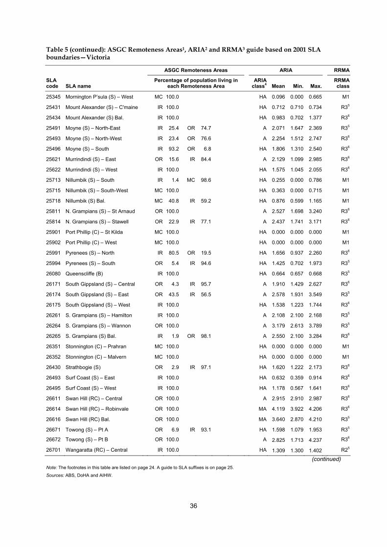
36
Table 5 (continued): ASGC Remoteness Areas1, ARIA2 and RRMA3 guide based on 2001 SLA boundaries—Victoria
ASGC Remoteness Areas ARIA RRMA
SLA code SLA name
Percentage of population living in each Remoteness Area
ARIA class4
Mean
Min. Max.
RRMA class
25345 Mornington P’sula (S) – West MC 100.0 HA 0.096 0.000 0.665 M1
25431 Mount Alexander (S) – C'maine IR 100.0 HA 0.712 0.710 0.734 R35
25434 Mount Alexander (S) Bal. IR 100.0 HA 0.983 0.702 1.377 R36
25491 Moyne (S) – North-East IR 25.4 OR 74.7 A 2.071 1.647 2.369 R35
25493 Moyne (S) – North-West IR 23.4 OR 76.6 A 2.254 1.512 2.747 R36
25496 Moyne (S) – South IR 93.2 OR 6.8 HA 1.806 1.310 2.540 R36
25621 Murrindindi (S) – East OR 15.6 IR 84.4 A 2.129 1.099 2.985 R36
25622 Murrindindi (S) – West IR 100.0 HA 1.575 1.045 2.055 R36
25713 Nillumbik (S) – South IR 1.4 MC 98.6 HA 0.255 0.000 0.786 M1
25715 Nillumbik (S) – South-West MC 100.0 HA 0.363 0.000 0.715 M1
25718 Nillumbik (S) Bal. MC 40.8 IR 59.2 HA 0.876 0.599 1.165 M1
25811 N. Grampians (S) – St Arnaud OR 100.0 A 2.527 1.698 3.240 R36
25814 N. Grampians (S) – Stawell OR 22.9 IR 77.1 A 2.437 1.741 3.171 R36
25901 Port Phillip (C) – St Kilda MC 100.0 HA 0.000 0.000 0.000 M1
25902 Port Phillip (C) – West MC 100.0 HA 0.000 0.000 0.000 M1
25991 Pyrenees (S) – North IR 80.5 OR 19.5 HA 1.656 0.937 2.260 R36
25994 Pyrenees (S) – South OR 5.4 IR 94.6 HA 1.425 0.702 1.973 R35
26080 Queenscliffe (B) IR 100.0 HA 0.664 0.657 0.668 R35
26171 South Gippsland (S) – Central OR 4.3 IR 95.7 A 1.910 1.429 2.627 R36
26174 South Gippsland (S) – East OR 43.5 IR 56.5 A 2.578 1.931 3.549 R35
26175 South Gippsland (S) – West IR 100.0 HA 1.538 1.223 1.744 R36
26261 S. Grampians (S) – Hamilton IR 100.0 A 2.108 2.100 2.168 R35
26264 S. Grampians (S) – Wannon OR 100.0 A 3.179 2.613 3.789 R35
26265 S. Grampians (S) Bal. IR 1.9 OR 98.1 A 2.550 2.100 3.284 R36
26351 Stonnington (C) – Prahran MC 100.0 HA 0.000 0.000 0.000 M1
26352 Stonnington (C) – Malvern MC 100.0 HA 0.000 0.000 0.000 M1
26430 Strathbogie (S) OR 2.9 IR 97.1 HA 1.620 1.222 2.173 R36
26493 Surf Coast (S) – East IR 100.0 HA 0.632 0.359 0.914 R36
26495 Surf Coast (S) – West IR 100.0 HA 1.178 0.567 1.641 R36
26611 Swan Hill (RC) – Central OR 100.0 A 2.915 2.910 2.987 R36
26614 Swan Hill (RC) – Robinvale OR 100.0 MA 4.119 3.922 4.206 R36
26616 Swan Hill (RC) Bal. OR 100.0 MA 3.640 2.870 4.210 R35
26671 Towong (S) – Pt A OR 6.9 IR 93.1 HA 1.598 1.079 1.953 R35
26672 Towong (S) – Pt B OR 100.0 A 2.825 1.713 4.237 R36
26701 Wangaratta (RC) – Central IR 100.0 HA 1.309 1.300 1.402 R25
(continued) Note: The footnotes in this table are listed on page 24. A guide to SLA suffixes is on page 25.
Sources: ABS, DoHA and AIHW.
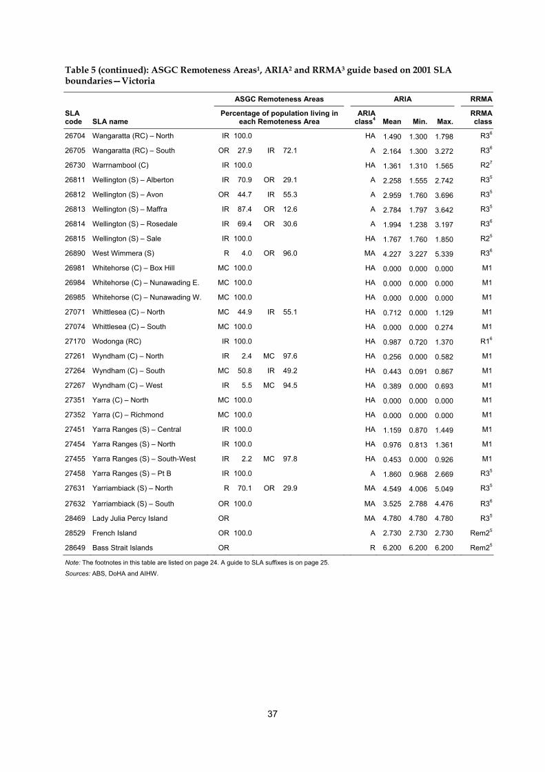
37
Table 5 (continued): ASGC Remoteness Areas1, ARIA2 and RRMA3 guide based on 2001 SLA boundaries—Victoria
ASGC Remoteness Areas ARIA RRMA
SLA code SLA name
Percentage of population living in each Remoteness Area
ARIA class4
Mean
Min. Max.
RRMA class
26704 Wangaratta (RC) – North IR 100.0 HA 1.490 1.300 1.798 R36
26705 Wangaratta (RC) – South OR 27.9 IR 72.1 A 2.164 1.300 3.272 R36
26730 Warrnambool (C) IR 100.0 HA 1.361 1.310 1.565 R27
26811 Wellington (S) – Alberton IR 70.9 OR 29.1 A 2.258 1.555 2.742 R35
26812 Wellington (S) – Avon OR 44.7 IR 55.3 A 2.959 1.760 3.696 R35
26813 Wellington (S) – Maffra IR 87.4 OR 12.6 A 2.784 1.797 3.642 R35
26814 Wellington (S) – Rosedale IR 69.4 OR 30.6 A 1.994 1.238 3.197 R36
26815 Wellington (S) – Sale IR 100.0 HA 1.767 1.760 1.850 R25
26890 West Wimmera (S) R 4.0 OR 96.0 MA 4.227 3.227 5.339 R36
26981 Whitehorse (C) – Box Hill MC 100.0 HA 0.000 0.000 0.000 M1
26984 Whitehorse (C) – Nunawading E. MC 100.0 HA 0.000 0.000 0.000 M1
26985 Whitehorse (C) – Nunawading W. MC 100.0 HA 0.000 0.000 0.000 M1
27071 Whittlesea (C) – North MC 44.9 IR 55.1 HA 0.712 0.000 1.129 M1
27074 Whittlesea (C) – South MC 100.0 HA 0.000 0.000 0.274 M1
27170 Wodonga (RC) IR 100.0 HA 0.987 0.720 1.370 R16
27261 Wyndham (C) – North IR 2.4 MC 97.6 HA 0.256 0.000 0.582 M1
27264 Wyndham (C) – South MC 50.8 IR 49.2 HA 0.443 0.091 0.867 M1
27267 Wyndham (C) – West IR 5.5 MC 94.5 HA 0.389 0.000 0.693 M1
27351 Yarra (C) – North MC 100.0 HA 0.000 0.000 0.000 M1
27352 Yarra (C) – Richmond MC 100.0 HA 0.000 0.000 0.000 M1
27451 Yarra Ranges (S) – Central IR 100.0 HA 1.159 0.870 1.449 M1
27454 Yarra Ranges (S) – North IR 100.0 HA 0.976 0.813 1.361 M1
27455 Yarra Ranges (S) – South-West IR 2.2 MC 97.8 HA 0.453 0.000 0.926 M1
27458 Yarra Ranges (S) – Pt B IR 100.0 A 1.860 0.968 2.669 R35
27631 Yarriambiack (S) – North R 70.1 OR 29.9 MA 4.549 4.006 5.049 R35
27632 Yarriambiack (S) – South OR 100.0 MA 3.525 2.788 4.476 R36
28469 Lady Julia Percy Island OR MA 4.780 4.780 4.780 R35
28529 French Island OR 100.0 A 2.730 2.730 2.730 Rem25
28649 Bass Strait Islands OR R 6.200 6.200 6.200 Rem25
Note: The footnotes in this table are listed on page 24. A guide to SLA suffixes is on page 25.
Sources: ABS, DoHA and AIHW.
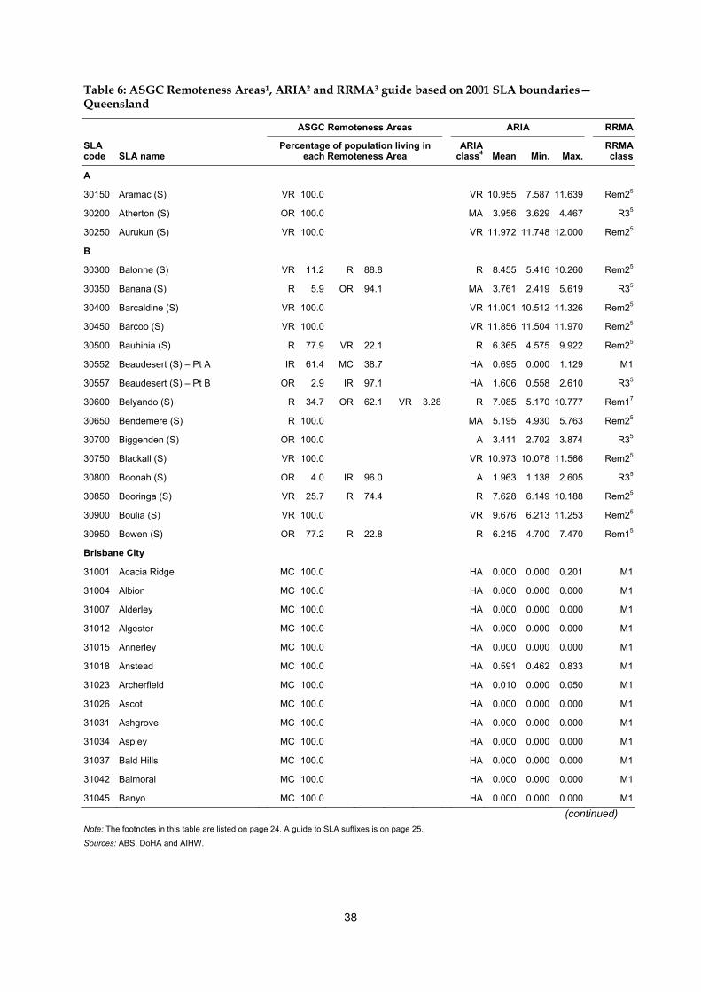
38
Table 6: ASGC Remoteness Areas1, ARIA2 and RRMA3 guide based on 2001 SLA boundaries—Queensland
ASGC Remoteness Areas ARIA RRMA
SLA code SLA name
Percentage of population living in each Remoteness Area
ARIA class4
Mean
Min. Max.
RRMA class
A
30150 Aramac (S) VR 100.0 VR 10.955 7.587 11.639 Rem25
30200 Atherton (S) OR 100.0 MA 3.956 3.629 4.467 R35
30250 Aurukun (S) VR 100.0 VR 11.972 11.748 12.000 Rem25
B
30300 Balonne (S) VR 11.2 R 88.8 R 8.455 5.416 10.260 Rem25
30350 Banana (S) R 5.9 OR 94.1 MA 3.761 2.419 5.619 R35
30400 Barcaldine (S) VR 100.0 VR 11.001 10.512 11.326 Rem25
30450 Barcoo (S) VR 100.0 VR 11.856 11.504 11.970 Rem25
30500 Bauhinia (S) R 77.9 VR 22.1 R 6.365 4.575 9.922 Rem25
30552 Beaudesert (S) – Pt A IR 61.4 MC 38.7 HA 0.695 0.000 1.129 M1
30557 Beaudesert (S) – Pt B OR 2.9 IR 97.1 HA 1.606 0.558 2.610 R35
30600 Belyando (S) R 34.7 OR 62.1 VR 3.28 R 7.085 5.170 10.777 Rem17
30650 Bendemere (S) R 100.0 MA 5.195 4.930 5.763 Rem25
30700 Biggenden (S) OR 100.0 A 3.411 2.702 3.874 R35
30750 Blackall (S) VR 100.0 VR 10.973 10.078 11.566 Rem25
30800 Boonah (S) OR 4.0 IR 96.0 A 1.963 1.138 2.605 R35
30850 Booringa (S) VR 25.7 R 74.4 R 7.628 6.149 10.188 Rem25
30900 Boulia (S) VR 100.0 VR 9.676 6.213 11.253 Rem25
30950 Bowen (S) OR 77.2 R 22.8 R 6.215 4.700 7.470 Rem15
Brisbane City
31001 Acacia Ridge MC 100.0 HA 0.000 0.000 0.201 M1
31004 Albion MC 100.0 HA 0.000 0.000 0.000 M1
31007 Alderley MC 100.0 HA 0.000 0.000 0.000 M1
31012 Algester MC 100.0 HA 0.000 0.000 0.000 M1
31015 Annerley MC 100.0 HA 0.000 0.000 0.000 M1
31018 Anstead MC 100.0 HA 0.591 0.462 0.833 M1
31023 Archerfield MC 100.0 HA 0.010 0.000 0.050 M1
31026 Ascot MC 100.0 HA 0.000 0.000 0.000 M1
31031 Ashgrove MC 100.0 HA 0.000 0.000 0.000 M1
31034 Aspley MC 100.0 HA 0.000 0.000 0.000 M1
31037 Bald Hills MC 100.0 HA 0.000 0.000 0.000 M1
31042 Balmoral MC 100.0 HA 0.000 0.000 0.000 M1
31045 Banyo MC 100.0 HA 0.000 0.000 0.000 M1
(continued) Note: The footnotes in this table are listed on page 24. A guide to SLA suffixes is on page 25.
Sources: ABS, DoHA and AIHW.
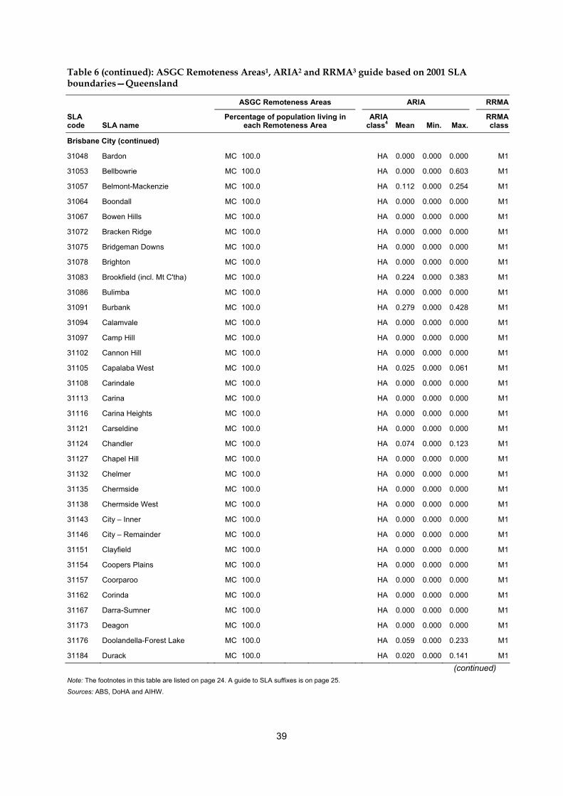
39
Table 6 (continued): ASGC Remoteness Areas1, ARIA2 and RRMA3 guide based on 2001 SLA boundaries—Queensland
ASGC Remoteness Areas ARIA RRMA
SLA code SLA name
Percentage of population living in each Remoteness Area
ARIA class4
Mean
Min. Max.
RRMA class
Brisbane City (continued)
31048 Bardon MC 100.0 HA 0.000 0.000 0.000 M1
31053 Bellbowrie MC 100.0 HA 0.000 0.000 0.603 M1
31057 Belmont-Mackenzie MC 100.0 HA 0.112 0.000 0.254 M1
31064 Boondall MC 100.0 HA 0.000 0.000 0.000 M1
31067 Bowen Hills MC 100.0 HA 0.000 0.000 0.000 M1
31072 Bracken Ridge MC 100.0 HA 0.000 0.000 0.000 M1
31075 Bridgeman Downs MC 100.0 HA 0.000 0.000 0.000 M1
31078 Brighton MC 100.0 HA 0.000 0.000 0.000 M1
31083 Brookfield (incl. Mt C'tha) MC 100.0 HA 0.224 0.000 0.383 M1
31086 Bulimba MC 100.0 HA 0.000 0.000 0.000 M1
31091 Burbank MC 100.0 HA 0.279 0.000 0.428 M1
31094 Calamvale MC 100.0 HA 0.000 0.000 0.000 M1
31097 Camp Hill MC 100.0 HA 0.000 0.000 0.000 M1
31102 Cannon Hill MC 100.0 HA 0.000 0.000 0.000 M1
31105 Capalaba West MC 100.0 HA 0.025 0.000 0.061 M1
31108 Carindale MC 100.0 HA 0.000 0.000 0.000 M1
31113 Carina MC 100.0 HA 0.000 0.000 0.000 M1
31116 Carina Heights MC 100.0 HA 0.000 0.000 0.000 M1
31121 Carseldine MC 100.0 HA 0.000 0.000 0.000 M1
31124 Chandler MC 100.0 HA 0.074 0.000 0.123 M1
31127 Chapel Hill MC 100.0 HA 0.000 0.000 0.000 M1
31132 Chelmer MC 100.0 HA 0.000 0.000 0.000 M1
31135 Chermside MC 100.0 HA 0.000 0.000 0.000 M1
31138 Chermside West MC 100.0 HA 0.000 0.000 0.000 M1
31143 City – Inner MC 100.0 HA 0.000 0.000 0.000 M1
31146 City – Remainder MC 100.0 HA 0.000 0.000 0.000 M1
31151 Clayfield MC 100.0 HA 0.000 0.000 0.000 M1
31154 Coopers Plains MC 100.0 HA 0.000 0.000 0.000 M1
31157 Coorparoo MC 100.0 HA 0.000 0.000 0.000 M1
31162 Corinda MC 100.0 HA 0.000 0.000 0.000 M1
31167 Darra-Sumner MC 100.0 HA 0.000 0.000 0.000 M1
31173 Deagon MC 100.0 HA 0.000 0.000 0.000 M1
31176 Doolandella-Forest Lake MC 100.0 HA 0.059 0.000 0.233 M1
31184 Durack MC 100.0 HA 0.020 0.000 0.141 M1
(continued) Note: The footnotes in this table are listed on page 24. A guide to SLA suffixes is on page 25.
Sources: ABS, DoHA and AIHW.

40
Table 6 (continued): ASGC Remoteness Areas1, ARIA2 and RRMA3 guide based on 2001 SLA boundaries—Queensland
ASGC Remoteness Areas ARIA RRMA
SLA code SLA name
Percentage of population living in each Remoteness Area
ARIA class4
Mean
Min. Max.
RRMA class
Brisbane City (continued)
31187 Dutton Park MC 100.0 HA 0.000 0.000 0.000 M1
31195 East Brisbane MC 100.0 HA 0.000 0.000 0.000 M1
31198 Eight Mile Plains MC 100.0 HA 0.043 0.000 0.256 M1
31203 Ellen Grove MC 100.0 HA 0.000 0.000 0.000 M1
31206 Enoggera MC 100.0 HA 0.000 0.000 0.000 M1
31211 Everton Park MC 100.0 HA 0.000 0.000 0.000 M1
31214 Fairfield MC 100.0 HA 0.000 0.000 0.000 M1
31217 Ferny Grove MC 100.0 HA 0.000 0.000 0.061 M1
31222 Fig Tree Pocket MC 100.0 HA 0.000 0.000 0.000 M1
31228 Fortitude Valley – Inner MC 100.0 HA 0.000 0.000 0.000 M1
31233 Fortitude Valley – Remainder MC 100.0 HA 0.000 0.000 0.000 M1
31236 Geebung MC 100.0 HA 0.000 0.000 0.000 M1
31241 Graceville MC 100.0 HA 0.000 0.000 0.000 M1
31244 Grange MC 100.0 HA 0.000 0.000 0.000 M1
31247 Greenslopes MC 100.0 HA 0.000 0.000 0.000 M1
31252 Gumdale MC 100.0 HA 0.000 0.000 0.000 M1
31255 Hamilton MC 100.0 HA 0.000 0.000 0.000 M1
31258 Hawthorne MC 100.0 HA 0.000 0.000 0.000 M1
31265 Hemmant-Lytton MC 100.0 HA 0.000 0.000 0.000 M1
31271 Hendra MC 100.0 HA 0.000 0.000 0.000 M1
31274 Herston MC 100.0 HA 0.000 0.000 0.000 M1
31277 Highgate Hill MC 100.0 HA 0.000 0.000 0.000 M1
31282 Holland Park MC 100.0 HA 0.000 0.000 0.000 M1
31285 Holland Park West MC 100.0 HA 0.000 0.000 0.000 M1
31288 Inala MC 100.0 HA 0.000 0.000 0.000 M1
31293 Indooroopilly MC 100.0 HA 0.000 0.000 0.000 M1
31296 Jamboree Heights MC 100.0 HA 0.000 0.000 0.000 M1
31301 Jindalee MC 100.0 HA 0.000 0.000 0.000 M1
31304 Kangaroo Point MC 100.0 HA 0.000 0.000 0.000 M1
31306 Karana Downs-Lake Manchester
IR 9.4 MC 90.6 HA 0.843 0.499 1.267 M1
31312 Kedron MC 100.0 HA 0.000 0.000 0.000 M1
31315 Kelvin Grove MC 100.0 HA 0.000 0.000 0.000 M1
31318 Kenmore MC 100.0 HA 0.000 0.000 0.000 M1
(continued) Note: The footnotes in this table are listed on page 24. A guide to SLA suffixes is on page 25.
Sources: ABS, DoHA and AIHW.

41
Table 6 (continued): ASGC Remoteness Areas1, ARIA2 and RRMA3 guide based on 2001 SLA boundaries—Queensland
ASGC Remoteness Areas ARIA RRMA
SLA code SLA name
Percentage of population living in each Remoteness Area
ARIA class4
Mean
Min. Max.
RRMA class
Brisbane City (continued)
31323 Kenmore Hills MC 100.0 HA 0.000 0.000 0.000 M1
31326 Keperra MC 100.0 HA 0.009 0.000 0.065 M1
31331 Kuraby MC 100.0 HA 0.058 0.000 0.288 M1
31337 Lota MC 100.0 HA 0.000 0.000 0.000 M1
31345 Lutwyche MC 100.0 HA 0.000 0.000 0.000 M1
31353 McDowall MC 100.0 HA 0.000 0.000 0.000 M1
31356 MacGregor MC 100.0 HA 0.000 0.000 0.000 M1
31364 Manly MC 100.0 HA 0.000 0.000 0.000 M1
31367 Manly West MC 100.0 HA 0.000 0.000 0.000 M1
31372 Mansfield MC 100.0 HA 0.000 0.000 0.000 M1
31375 Middle Park MC 100.0 HA 0.000 0.000 0.000 M1
31378 Milton MC 100.0 HA 0.000 0.000 0.000 M1
31383 Mitchelton MC 100.0 HA 0.000 0.000 0.000 M1
31386 Moggill MC 100.0 HA 0.473 0.005 0.904 M1
31391 Moorooka MC 100.0 HA 0.000 0.000 0.000 M1
31394 Moreton Island OR 0.0 R 100.0 MA 5.010 5.010 5.010 M1
31397 Morningside MC 100.0 HA 0.000 0.000 0.000 M1
31402 Mount Gravatt MC 100.0 HA 0.000 0.000 0.000 M1
31405 Mount Gravatt East MC 100.0 HA 0.000 0.000 0.000 M1
31408 Mount Ommaney MC 100.0 HA 0.000 0.000 0.000 M1
31413 Murarrie MC 100.0 HA 0.000 0.000 0.000 M1
31416 Nathan MC 100.0 HA 0.000 0.000 0.000 M1
31421 New Farm MC 100.0 HA 0.000 0.000 0.000 M1
31424 Newmarket MC 100.0 HA 0.000 0.000 0.000 M1
31427 Newstead MC 100.0 HA 0.000 0.000 0.000 M1
31432 Norman Park MC 100.0 HA 0.000 0.000 0.000 M1
31435 Northgate MC 100.0 HA 0.000 0.000 0.000 M1
31438 Nudgee MC 100.0 HA 0.000 0.000 0.000 M1
31443 Nudgee Beach MC 100.0 HA 0.000 0.000 0.000 M1
31446 Nundah MC 100.0 HA 0.000 0.000 0.000 M1
31451 Oxley MC 100.0 HA 0.000 0.000 0.000 M1
31454 Paddington MC 100.0 HA 0.000 0.000 0.000 M1
31456 Pallara-Heathwood-Larapinta MC 100.0 HA 0.184 0.000 0.403 M1
31463 Parkinson-Drewvale MC 100.0 HA 0.000 0.000 0.000 M1
(continued) Note: The footnotes in this table are listed on page 24. A guide to SLA suffixes is on page 25.
Sources: ABS, DoHA and AIHW.
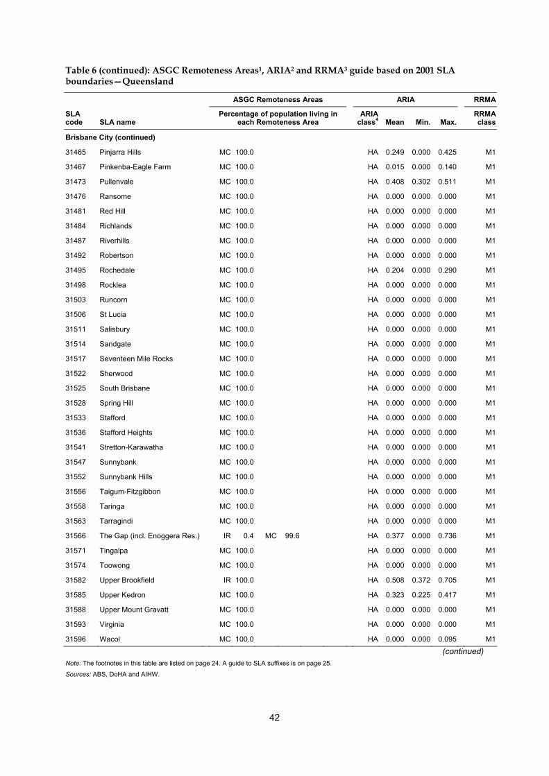
42
Table 6 (continued): ASGC Remoteness Areas1, ARIA2 and RRMA3 guide based on 2001 SLA boundaries—Queensland
ASGC Remoteness Areas ARIA RRMA
SLA code SLA name
Percentage of population living in each Remoteness Area
ARIA class4
Mean
Min. Max.
RRMA class
Brisbane City (continued)
31465 Pinjarra Hills MC 100.0 HA 0.249 0.000 0.425 M1
31467 Pinkenba-Eagle Farm MC 100.0 HA 0.015 0.000 0.140 M1
31473 Pullenvale MC 100.0 HA 0.408 0.302 0.511 M1
31476 Ransome MC 100.0 HA 0.000 0.000 0.000 M1
31481 Red Hill MC 100.0 HA 0.000 0.000 0.000 M1
31484 Richlands MC 100.0 HA 0.000 0.000 0.000 M1
31487 Riverhills MC 100.0 HA 0.000 0.000 0.000 M1
31492 Robertson MC 100.0 HA 0.000 0.000 0.000 M1
31495 Rochedale MC 100.0 HA 0.204 0.000 0.290 M1
31498 Rocklea MC 100.0 HA 0.000 0.000 0.000 M1
31503 Runcorn MC 100.0 HA 0.000 0.000 0.000 M1
31506 St Lucia MC 100.0 HA 0.000 0.000 0.000 M1
31511 Salisbury MC 100.0 HA 0.000 0.000 0.000 M1
31514 Sandgate MC 100.0 HA 0.000 0.000 0.000 M1
31517 Seventeen Mile Rocks MC 100.0 HA 0.000 0.000 0.000 M1
31522 Sherwood MC 100.0 HA 0.000 0.000 0.000 M1
31525 South Brisbane MC 100.0 HA 0.000 0.000 0.000 M1
31528 Spring Hill MC 100.0 HA 0.000 0.000 0.000 M1
31533 Stafford MC 100.0 HA 0.000 0.000 0.000 M1
31536 Stafford Heights MC 100.0 HA 0.000 0.000 0.000 M1
31541 Stretton-Karawatha MC 100.0 HA 0.000 0.000 0.000 M1
31547 Sunnybank MC 100.0 HA 0.000 0.000 0.000 M1
31552 Sunnybank Hills MC 100.0 HA 0.000 0.000 0.000 M1
31556 Taigum-Fitzgibbon MC 100.0 HA 0.000 0.000 0.000 M1
31558 Taringa MC 100.0 HA 0.000 0.000 0.000 M1
31563 Tarragindi MC 100.0 HA 0.000 0.000 0.000 M1
31566 The Gap (incl. Enoggera Res.) IR 0.4 MC 99.6 HA 0.377 0.000 0.736 M1
31571 Tingalpa MC 100.0 HA 0.000 0.000 0.000 M1
31574 Toowong MC 100.0 HA 0.000 0.000 0.000 M1
31582 Upper Brookfield IR 100.0 HA 0.508 0.372 0.705 M1
31585 Upper Kedron MC 100.0 HA 0.323 0.225 0.417 M1
31588 Upper Mount Gravatt MC 100.0 HA 0.000 0.000 0.000 M1
31593 Virginia MC 100.0 HA 0.000 0.000 0.000 M1
31596 Wacol MC 100.0 HA 0.000 0.000 0.095 M1
(continued) Note: The footnotes in this table are listed on page 24. A guide to SLA suffixes is on page 25.
Sources: ABS, DoHA and AIHW.
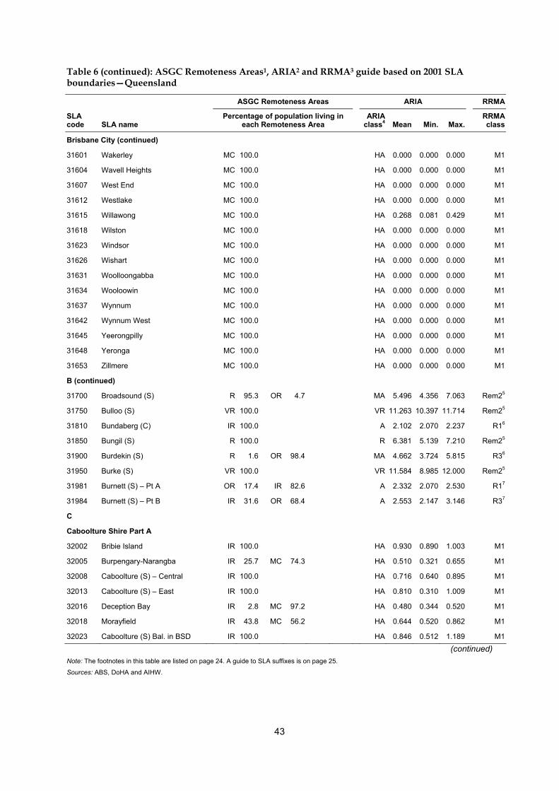
43
Table 6 (continued): ASGC Remoteness Areas1, ARIA2 and RRMA3 guide based on 2001 SLA boundaries—Queensland
ASGC Remoteness Areas ARIA RRMA
SLA code SLA name
Percentage of population living in each Remoteness Area
ARIA class4
Mean
Min. Max.
RRMA class
Brisbane City (continued)
31601 Wakerley MC 100.0 HA 0.000 0.000 0.000 M1
31604 Wavell Heights MC 100.0 HA 0.000 0.000 0.000 M1
31607 West End MC 100.0 HA 0.000 0.000 0.000 M1
31612 Westlake MC 100.0 HA 0.000 0.000 0.000 M1
31615 Willawong MC 100.0 HA 0.268 0.081 0.429 M1
31618 Wilston MC 100.0 HA 0.000 0.000 0.000 M1
31623 Windsor MC 100.0 HA 0.000 0.000 0.000 M1
31626 Wishart MC 100.0 HA 0.000 0.000 0.000 M1
31631 Woolloongabba MC 100.0 HA 0.000 0.000 0.000 M1
31634 Wooloowin MC 100.0 HA 0.000 0.000 0.000 M1
31637 Wynnum MC 100.0 HA 0.000 0.000 0.000 M1
31642 Wynnum West MC 100.0 HA 0.000 0.000 0.000 M1
31645 Yeerongpilly MC 100.0 HA 0.000 0.000 0.000 M1
31648 Yeronga MC 100.0 HA 0.000 0.000 0.000 M1
31653 Zillmere MC 100.0 HA 0.000 0.000 0.000 M1
B (continued)
31700 Broadsound (S) R 95.3 OR 4.7 MA 5.496 4.356 7.063 Rem25
31750 Bulloo (S) VR 100.0 VR 11.263 10.397 11.714 Rem25
31810 Bundaberg (C) IR 100.0 A 2.102 2.070 2.237 R16
31850 Bungil (S) R 100.0 R 6.381 5.139 7.210 Rem25
31900 Burdekin (S) R 1.6 OR 98.4 MA 4.662 3.724 5.815 R36
31950 Burke (S) VR 100.0 VR 11.584 8.985 12.000 Rem25
31981 Burnett (S) – Pt A OR 17.4 IR 82.6 A 2.332 2.070 2.530 R17
31984 Burnett (S) – Pt B IR 31.6 OR 68.4 A 2.553 2.147 3.146 R37
C
Caboolture Shire Part A
32002 Bribie Island IR 100.0 HA 0.930 0.890 1.003 M1
32005 Burpengary-Narangba IR 25.7 MC 74.3 HA 0.510 0.321 0.655 M1
32008 Caboolture (S) – Central IR 100.0 HA 0.716 0.640 0.895 M1
32013 Caboolture (S) – East IR 100.0 HA 0.810 0.310 1.009 M1
32016 Deception Bay IR 2.8 MC 97.2 HA 0.480 0.344 0.520 M1
32018 Morayfield IR 43.8 MC 56.2 HA 0.644 0.520 0.862 M1
32023 Caboolture (S) Bal. in BSD IR 100.0 HA 0.846 0.512 1.189 M1
(continued) Note: The footnotes in this table are listed on page 24. A guide to SLA suffixes is on page 25.
Sources: ABS, DoHA and AIHW.

44
Table 6 (continued): ASGC Remoteness Areas1, ARIA2 and RRMA3 guide based on 2001 SLA boundaries—Queensland
ASGC Remoteness Areas ARIA RRMA
SLA code SLA name
Percentage of population living in each Remoteness Area
ARIA class4
Mean
Min. Max.
RRMA class
C (continued)
32031 Caboolture (S) – Pt B IR 100.0 HA 1.165 0.858 1.481 R36
32062 Cairns (C) – Barron OR 100.0 A 3.215 3.000 3.543 R16
32065 Cairns (C) – Central Suburbs OR 100.0 A 3.005 3.000 3.053 R16
32066 Cairns (C) – City OR 100.0 A 3.000 3.000 3.000 R16
32068 Cairns (C) – Mt Whitfield OR 100.0 A 3.019 3.000 3.132 R16
32072 Cairns (C) – Northern Suburbs OR 100.0 A 3.480 3.359 3.552 R16
32074 Cairns (C) – Trinity OR 100.0 A 3.249 3.000 3.923 R16
32076 Cairns (C) – Western Suburbs OR 100.0 A 3.000 3.000 3.000 R16
32078 Cairns (C) – Pt B R 0.0 OR 100.0 MA 3.898 3.234 4.318 R36
32101 Calliope (S) – Pt A IR 100.0 A 2.094 1.927 2.536 R35
32104 Calliope (S) – Pt B R 11.2 OR 88.8 A 2.609 1.864 3.994 R35
32132 Caloundra (C) – Caloundra N. IR 100.0 HA 0.661 0.600 0.766 R26
32133 Caloundra (C) – Caloundra S. IR 100.0 HA 0.761 0.600 0.910 R26
32135 Caloundra (C) – Kawana IR 100.0 HA 0.689 0.650 0.761 R26
32136 Caloundra (C) – Hinterland IR 100.0 HA 1.358 0.893 1.886 R36
32138 Caloundra (C) – Rail Corridor IR 100.0 HA 0.898 0.689 1.114 R36
32151 Cambooya (S) – Pt A IR 100.0 HA 0.638 0.503 0.790 R36
32154 Cambooya (S) – Pt B IR 100.0 HA 1.029 0.585 1.347 R36
32200 Cardwell (S) OR 83.1 R 16.9 MA 5.564 4.506 5.960 R35
32250 Carpentaria (S) VR 100.0 VR 11.510 10.346 12.000 Rem25
32300 Charters Towers (C) OR 100.0 MA 4.551 4.550 4.576 R35
32350 Chinchilla (S) R 2.1 OR 97.9 MA 4.128 2.452 6.185 R35
32400 Clifton (S) IR 100.0 HA 1.454 1.182 1.847 R35
32450 Cloncurry (S) R 58.6 VR 41.4 R 8.953 6.258 11.079 Rem25
32501 Cook (S) (excl. Weipa) R 44.5 VR 55.5 VR 10.825 5.924 12.000 Rem25
32504 Cook (S) – Weipa only VR 100.0 VR 12.000 12.000 12.000 Rem25
32532 Cooloola (S) (excl. Gympie) OR 7.6 IR 92.5 A 1.552 1.520 1.756 R36
32535 Cooloola (S) – Gympie only IR 100.0 HA 1.847 1.425 2.669 R26
32551 Crows Nest (S) – Pt A IR 100.0 HA 0.709 0.492 0.983 R36
32554 Crows Nest (S) – Pt B IR 90.4 OR 9.6 HA 1.540 0.814 2.157 R36
32600 Croydon (S) VR 100.0 VR 11.328 10.664 11.798 Rem25
D–F
32650 Dalby (T) IR 100.0 HA 1.452 1.443 1.483 R35
32700 Dalrymple (S) VR 10.2 R 78.4 OR 11.4 R 6.380 3.340 10.513 Rem25
(continued) Note: The footnotes in this table are listed on page 24. A guide to SLA suffixes is on page 25.
Sources: ABS, DoHA and AIHW.
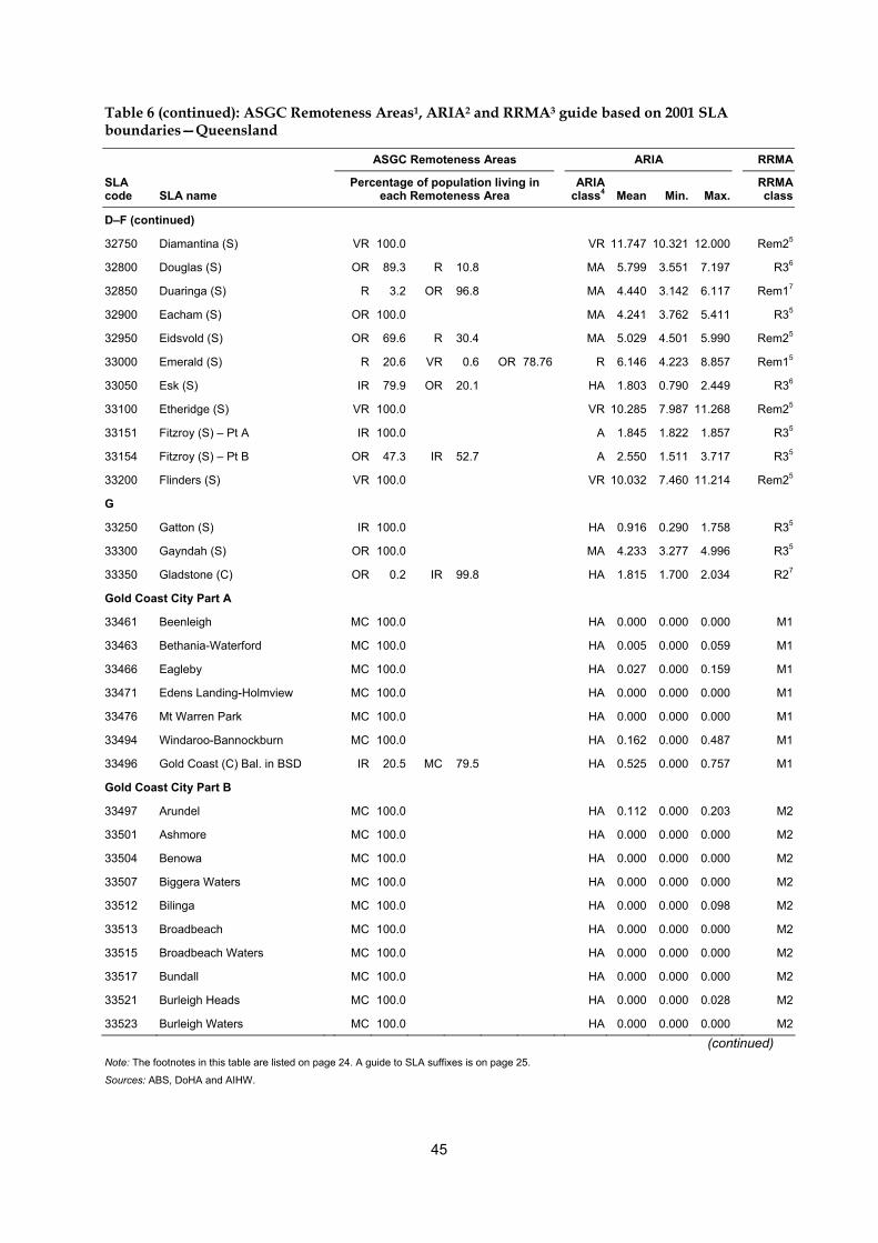
45
Table 6 (continued): ASGC Remoteness Areas1, ARIA2 and RRMA3 guide based on 2001 SLA boundaries—Queensland
ASGC Remoteness Areas ARIA RRMA
SLA code SLA name
Percentage of population living in each Remoteness Area
ARIA class4
Mean
Min. Max.
RRMA class
D–F (continued)
32750 Diamantina (S) VR 100.0 VR 11.747 10.321 12.000 Rem25
32800 Douglas (S) OR 89.3 R 10.8 MA 5.799 3.551 7.197 R36
32850 Duaringa (S) R 3.2 OR 96.8 MA 4.440 3.142 6.117 Rem17
32900 Eacham (S) OR 100.0 MA 4.241 3.762 5.411 R35
32950 Eidsvold (S) OR 69.6 R 30.4 MA 5.029 4.501 5.990 Rem25
33000 Emerald (S) R 20.6 VR 0.6 OR 78.76 R 6.146 4.223 8.857 Rem15
33050 Esk (S) IR 79.9 OR 20.1 HA 1.803 0.790 2.449 R36
33100 Etheridge (S) VR 100.0 VR 10.285 7.987 11.268 Rem25
33151 Fitzroy (S) – Pt A IR 100.0 A 1.845 1.822 1.857 R35
33154 Fitzroy (S) – Pt B OR 47.3 IR 52.7 A 2.550 1.511 3.717 R35
33200 Flinders (S) VR 100.0 VR 10.032 7.460 11.214 Rem25
G
33250 Gatton (S) IR 100.0 HA 0.916 0.290 1.758 R35
33300 Gayndah (S) OR 100.0 MA 4.233 3.277 4.996 R35
33350 Gladstone (C) OR 0.2 IR 99.8 HA 1.815 1.700 2.034 R27
Gold Coast City Part A
33461 Beenleigh MC 100.0 HA 0.000 0.000 0.000 M1
33463 Bethania-Waterford MC 100.0 HA 0.005 0.000 0.059 M1
33466 Eagleby MC 100.0 HA 0.027 0.000 0.159 M1
33471 Edens Landing-Holmview MC 100.0 HA 0.000 0.000 0.000 M1
33476 Mt Warren Park MC 100.0 HA 0.000 0.000 0.000 M1
33494 Windaroo-Bannockburn MC 100.0 HA 0.162 0.000 0.487 M1
33496 Gold Coast (C) Bal. in BSD IR 20.5 MC 79.5 HA 0.525 0.000 0.757 M1
Gold Coast City Part B
33497 Arundel MC 100.0 HA 0.112 0.000 0.203 M2
33501 Ashmore MC 100.0 HA 0.000 0.000 0.000 M2
33504 Benowa MC 100.0 HA 0.000 0.000 0.000 M2
33507 Biggera Waters MC 100.0 HA 0.000 0.000 0.000 M2
33512 Bilinga MC 100.0 HA 0.000 0.000 0.098 M2
33513 Broadbeach MC 100.0 HA 0.000 0.000 0.000 M2
33515 Broadbeach Waters MC 100.0 HA 0.000 0.000 0.000 M2
33517 Bundall MC 100.0 HA 0.000 0.000 0.000 M2
33521 Burleigh Heads MC 100.0 HA 0.000 0.000 0.028 M2
33523 Burleigh Waters MC 100.0 HA 0.000 0.000 0.000 M2
(continued) Note: The footnotes in this table are listed on page 24. A guide to SLA suffixes is on page 25.
Sources: ABS, DoHA and AIHW.
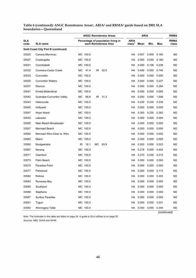
46
Table 6 (continued): ASGC Remoteness Areas1, ARIA2 and RRMA3 guide based on 2001 SLA boundaries—Queensland
ASGC Remoteness Areas ARIA RRMA
SLA code SLA name
Percentage of population living in each Remoteness Area
ARIA class4
Mean
Min. Max.
RRMA class
Gold Coast City Part B (continued)
33525 Carrara-Merrimac MC 100.0 HA 0.007 0.000 0.160 M2
33527 Coolangatta MC 100.0 HA 0.000 0.000 0.180 M2
33531 Coombabah MC 100.0 HA 0.000 0.106 0.238 M2
33532 Coomera-Cedar Creek MC 47.4 IR 52.6 HA 0.495 0.000 0.740 M2
33533 Currumbin MC 100.0 HA 0.000 0.000 0.000 M2
33535 Currumbin Waters MC 100.0 HA 0.000 0.000 0.237 M2
33537 Elanora MC 100.0 HA 0.000 0.000 0.264 M2
33541 Ernest-Molendinar MC 100.0 HA 0.000 0.000 0.065 M2
33542 Guanaba-Currumbin Valley MC 68.8 IR 31.3 HA 0.000 0.000 1.006 M2
33543 Helensvale MC 100.0 HA 0.230 0.230 0.230 M2
33545 Hollywell MC 100.0 HA 0.000 0.000 0.000 M2
33547 Hope Island MC 100.0 HA 0.300 0.230 0.362 M2
33553 Labrador MC 100.0 HA 0.000 0.000 0.000 M2
33555 Main Beach-Broadwater MC 100.0 HA 0.000 0.000 0.000 M2
33557 Mermaid Beach MC 100.0 HA 0.000 0.000 0.000 M2
33562 Mermaid Wtrs-Clear Is. Wtrs MC 100.0 HA 0.000 0.000 0.000 M2
33563 Miami MC 100.0 HA 0.000 0.000 0.000 M2
33565 Mudgeeraba IR 16.1 MC 83.9 HA 0.000 0.000 0.523 M2
33567 Nerang MC 100.0 HA 0.218 0.000 0.404 M2
33571 Oxenford MC 100.0 HA 0.270 0.230 0.315 M2
33573 Palm Beach MC 100.0 HA 0.000 0.000 0.000 M2
33575 Paradise Point MC 100.0 HA 0.000 0.000 0.000 M2
33577 Parkwood MC 100.0 HA 0.000 0.000 0.174 M2
33582 Robina MC 100.0 HA 0.000 0.000 0.303 M2
33583 Runaway Bay MC 100.0 HA 0.000 0.000 0.000 M2
33585 Southport MC 100.0 HA 0.000 0.000 0.000 M2
33586 Stephens MC 100.0 HA 0.000 0.000 0.000 M2
33587 Surfers Paradise MC 100.0 HA 0.000 0.000 0.000 M2
33591 Tugun MC 100.0 HA 0.000 0.000 0.031 M2
33593 Worongary-Tallai MC 100.0 HA 0.000 0.000 0.345 M2
(continued) Note: The footnotes in this table are listed on page 24. A guide to SLA suffixes is on page 25.
Sources: ABS, DoHA and AIHW.
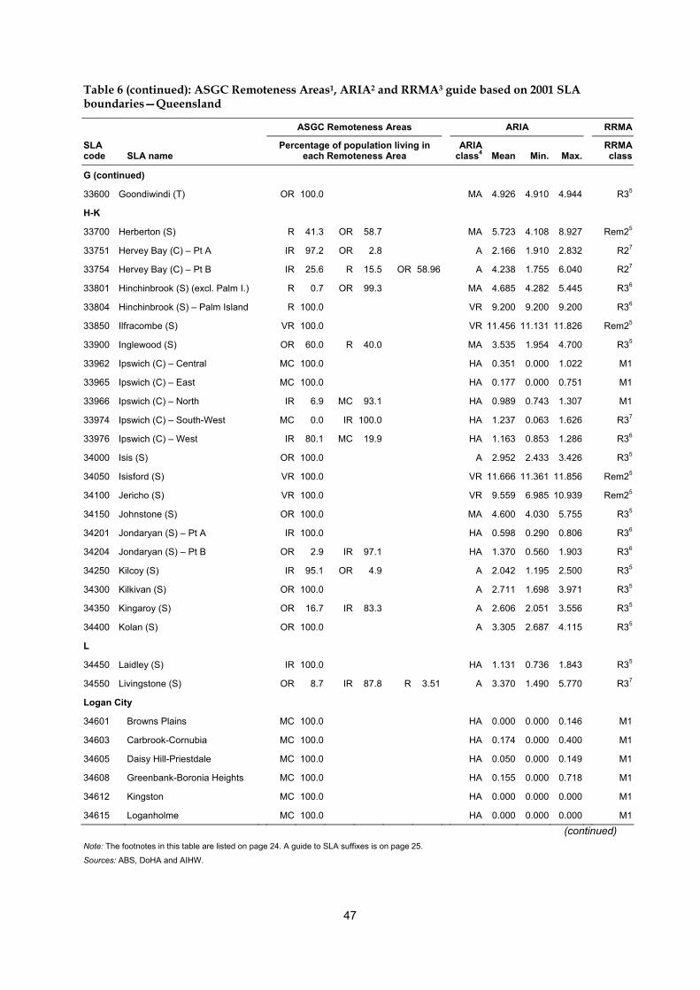
47
Table 6 (continued): ASGC Remoteness Areas1, ARIA2 and RRMA3 guide based on 2001 SLA boundaries—Queensland
ASGC Remoteness Areas ARIA RRMA
SLA code SLA name
Percentage of population living in each Remoteness Area
ARIA class4
Mean
Min. Max.
RRMA class
G (continued)
33600 Goondiwindi (T) OR 100.0 MA 4.926 4.910 4.944 R35
H-K
33700 Herberton (S) R 41.3 OR 58.7 MA 5.723 4.108 8.927 Rem25
33751 Hervey Bay (C) – Pt A IR 97.2 OR 2.8 A 2.166 1.910 2.832 R27
33754 Hervey Bay (C) – Pt B IR 25.6 R 15.5 OR 58.96 A 4.238 1.755 6.040 R27
33801 Hinchinbrook (S) (excl. Palm I.) R 0.7 OR 99.3 MA 4.685 4.282 5.445 R36
33804 Hinchinbrook (S) – Palm Island R 100.0 VR 9.200 9.200 9.200 R36
33850 Ilfracombe (S) VR 100.0 VR 11.456 11.131 11.826 Rem25
33900 Inglewood (S) OR 60.0 R 40.0 MA 3.535 1.954 4.700 R35
33962 Ipswich (C) – Central MC 100.0 HA 0.351 0.000 1.022 M1
33965 Ipswich (C) – East MC 100.0 HA 0.177 0.000 0.751 M1
33966 Ipswich (C) – North IR 6.9 MC 93.1 HA 0.989 0.743 1.307 M1
33974 Ipswich (C) – South-West MC 0.0 IR 100.0 HA 1.237 0.063 1.626 R37
33976 Ipswich (C) – West IR 80.1 MC 19.9 HA 1.163 0.853 1.286 R36
34000 Isis (S) OR 100.0 A 2.952 2.433 3.426 R35
34050 Isisford (S) VR 100.0 VR 11.666 11.361 11.856 Rem25
34100 Jericho (S) VR 100.0 VR 9.559 6.985 10.939 Rem25
34150 Johnstone (S) OR 100.0 MA 4.600 4.030 5.755 R35
34201 Jondaryan (S) – Pt A IR 100.0 HA 0.598 0.290 0.806 R36
34204 Jondaryan (S) – Pt B OR 2.9 IR 97.1 HA 1.370 0.560 1.903 R36
34250 Kilcoy (S) IR 95.1 OR 4.9 A 2.042 1.195 2.500 R35
34300 Kilkivan (S) OR 100.0 A 2.711 1.698 3.971 R35
34350 Kingaroy (S) OR 16.7 IR 83.3 A 2.606 2.051 3.556 R35
34400 Kolan (S) OR 100.0 A 3.305 2.687 4.115 R35
L
34450 Laidley (S) IR 100.0 HA 1.131 0.736 1.843 R35
34550 Livingstone (S) OR 8.7 IR 87.8 R 3.51 A 3.370 1.490 5.770 R37
Logan City
34601 Browns Plains MC 100.0 HA 0.000 0.000 0.146 M1
34603 Carbrook-Cornubia MC 100.0 HA 0.174 0.000 0.400 M1
34605 Daisy Hill-Priestdale MC 100.0 HA 0.050 0.000 0.149 M1
34608 Greenbank-Boronia Heights MC 100.0 HA 0.155 0.000 0.718 M1
34612 Kingston MC 100.0 HA 0.000 0.000 0.000 M1
34615 Loganholme MC 100.0 HA 0.000 0.000 0.000 M1
(continued) Note: The footnotes in this table are listed on page 24. A guide to SLA suffixes is on page 25.
Sources: ABS, DoHA and AIHW.
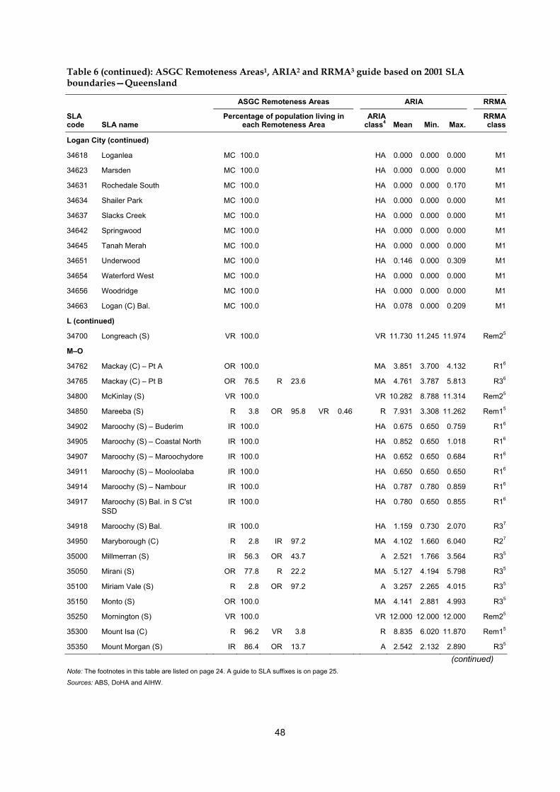
48
Table 6 (continued): ASGC Remoteness Areas1, ARIA2 and RRMA3 guide based on 2001 SLA boundaries—Queensland
ASGC Remoteness Areas ARIA RRMA
SLA code SLA name
Percentage of population living in each Remoteness Area
ARIA class4
Mean
Min. Max.
RRMA class
Logan City (continued)
34618 Loganlea MC 100.0 HA 0.000 0.000 0.000 M1
34623 Marsden MC 100.0 HA 0.000 0.000 0.000 M1
34631 Rochedale South MC 100.0 HA 0.000 0.000 0.170 M1
34634 Shailer Park MC 100.0 HA 0.000 0.000 0.000 M1
34637 Slacks Creek MC 100.0 HA 0.000 0.000 0.000 M1
34642 Springwood MC 100.0 HA 0.000 0.000 0.000 M1
34645 Tanah Merah MC 100.0 HA 0.000 0.000 0.000 M1
34651 Underwood MC 100.0 HA 0.146 0.000 0.309 M1
34654 Waterford West MC 100.0 HA 0.000 0.000 0.000 M1
34656 Woodridge MC 100.0 HA 0.000 0.000 0.000 M1
34663 Logan (C) Bal. MC 100.0 HA 0.078 0.000 0.209 M1
L (continued)
34700 Longreach (S) VR 100.0 VR 11.730 11.245 11.974 Rem25
M–O
34762 Mackay (C) – Pt A OR 100.0 MA 3.851 3.700 4.132 R16
34765 Mackay (C) – Pt B OR 76.5 R 23.6 MA 4.761 3.787 5.813 R36
34800 McKinlay (S) VR 100.0 VR 10.282 8.788 11.314 Rem25
34850 Mareeba (S) R 3.8 OR 95.8 VR 0.46 R 7.931 3.308 11.262 Rem15
34902 Maroochy (S) – Buderim IR 100.0 HA 0.675 0.650 0.759 R16
34905 Maroochy (S) – Coastal North IR 100.0 HA 0.852 0.650 1.018 R16
34907 Maroochy (S) – Maroochydore IR 100.0 HA 0.652 0.650 0.684 R16
34911 Maroochy (S) – Mooloolaba IR 100.0 HA 0.650 0.650 0.650 R16
34914 Maroochy (S) – Nambour IR 100.0 HA 0.787 0.780 0.859 R16
34917 Maroochy (S) Bal. in S C'st SSD
IR 100.0 HA 0.780 0.650 0.855 R16
34918 Maroochy (S) Bal. IR 100.0 HA 1.159 0.730 2.070 R37
34950 Maryborough (C) R 2.8 IR 97.2 MA 4.102 1.660 6.040 R27
35000 Millmerran (S) IR 56.3 OR 43.7 A 2.521 1.766 3.564 R35
35050 Mirani (S) OR 77.8 R 22.2 MA 5.127 4.194 5.798 R35
35100 Miriam Vale (S) R 2.8 OR 97.2 A 3.257 2.265 4.015 R35
35150 Monto (S) OR 100.0 MA 4.141 2.881 4.993 R35
35250 Mornington (S) VR 100.0 VR 12.000 12.000 12.000 Rem25
35300 Mount Isa (C) R 96.2 VR 3.8 R 8.835 6.020 11.870 Rem15
35350 Mount Morgan (S) IR 86.4 OR 13.7 A 2.542 2.132 2.890 R35
(continued) Note: The footnotes in this table are listed on page 24. A guide to SLA suffixes is on page 25.
Sources: ABS, DoHA and AIHW.

49
Table 6 (continued): ASGC Remoteness Areas1, ARIA2 and RRMA3 guide based on 2001 SLA boundaries—Queensland
ASGC Remoteness Areas ARIA RRMA
SLA code SLA name
Percentage of population living in each Remoteness Area
ARIA class4
Mean
Min. Max.
RRMA class
M–O (continued)
35450 Mundubbera (S) OR 79.4 R 20.6 MA 4.931 3.646 5.258 R35
35500 Murgon (S) OR 100.0 A 2.930 2.686 3.259 R35
35550 Murilla (S) OR 71.8 R 28.2 MA 4.811 3.764 5.833 Rem25
35600 Murweh (S) R 60.9 VR 39.1 VR 10.002 5.913 11.008 Rem25
35650 Nanango (S) IR 59.3 OR 40.7 A 2.164 2.015 2.740 R35
35700 Nebo (S) R 100.0 MA 5.506 4.118 6.736 Rem25
35752 Noosa (S) – Noosa-Noosaville IR 100.0 HA 0.882 0.880 0.894 R27
35755 Noosa (S) – Sunshine-Peregian
IR 100.0 HA 0.950 0.880 1.039 R27
35756 Noosa (S) – Tewantin IR 100.0 HA 0.884 0.880 0.928 R27
35758 Noosa (S) Bal. IR 100.0 HA 1.288 0.880 1.703 R27
P-Q
35800 Paroo (S) VR 100.0 VR 10.781 9.281 11.306 Rem25
35850 Peak Downs (S) R 100.0 R 6.327 4.524 7.382 Rem25
35900 Perry (S) OR 100.0 MA 3.990 3.050 4.928 Rem25
Pine Rivers Shire
35951 Albany Creek MC 100.0 HA 0.003 0.000 0.039 M1
35957 Bray Park MC 100.0 HA 0.000 0.000 0.036 M1
35958 Central Pine West IR 1.5 MC 98.5 HA 0.346 0.000 0.766 M1
35961 Dakabin-Kallangur-M. Downs MC 100.0 HA 0.050 0.000 0.334 M1
35963 Griffin-Mango Hill MC 100.0 HA 0.000 0.000 0.141 M1
35971 Hills District MC 100.0 HA 0.159 0.000 0.487 M1
35973 Lawnton MC 100.0 HA 0.000 0.000 0.000 M1
35974 Petrie MC 100.0 HA 0.000 0.000 0.000 M1
35978 Strathpine-Brendale MC 100.0 HA 0.022 0.000 0.068 M1
35988 Pine Rivers (S) Bal. MC 12.1 IR 87.9 HA 0.790 0.000 1.358 M1
Redcliffe City
36050 Pittsworth (S) IR 100.0 HA 1.509 0.956 1.869 R35
36150 Quilpie (S) VR 100.0 VR 11.431 10.731 11.857 Rem25
36201 Clontarf MC 100.0 HA 0.000 0.000 0.035 M1
36204 Margate-Woody Point MC 100.0 HA 0.000 0.000 0.000 M1
36206 Redcliffe-Scarborough MC 100.0 HA 0.000 0.000 0.000 M1
36208 Rothwell-Kippa-Ring MC 100.0 HA 0.000 0.000 0.043 M1
Redland Shire
36251 Alexandra Hills MC 100.0 HA 0.000 0.000 0.000 M1
(continued) Note: The footnotes in this table are listed on page 24. A guide to SLA suffixes is on page 25.
Sources: ABS, DoHA and AIHW.
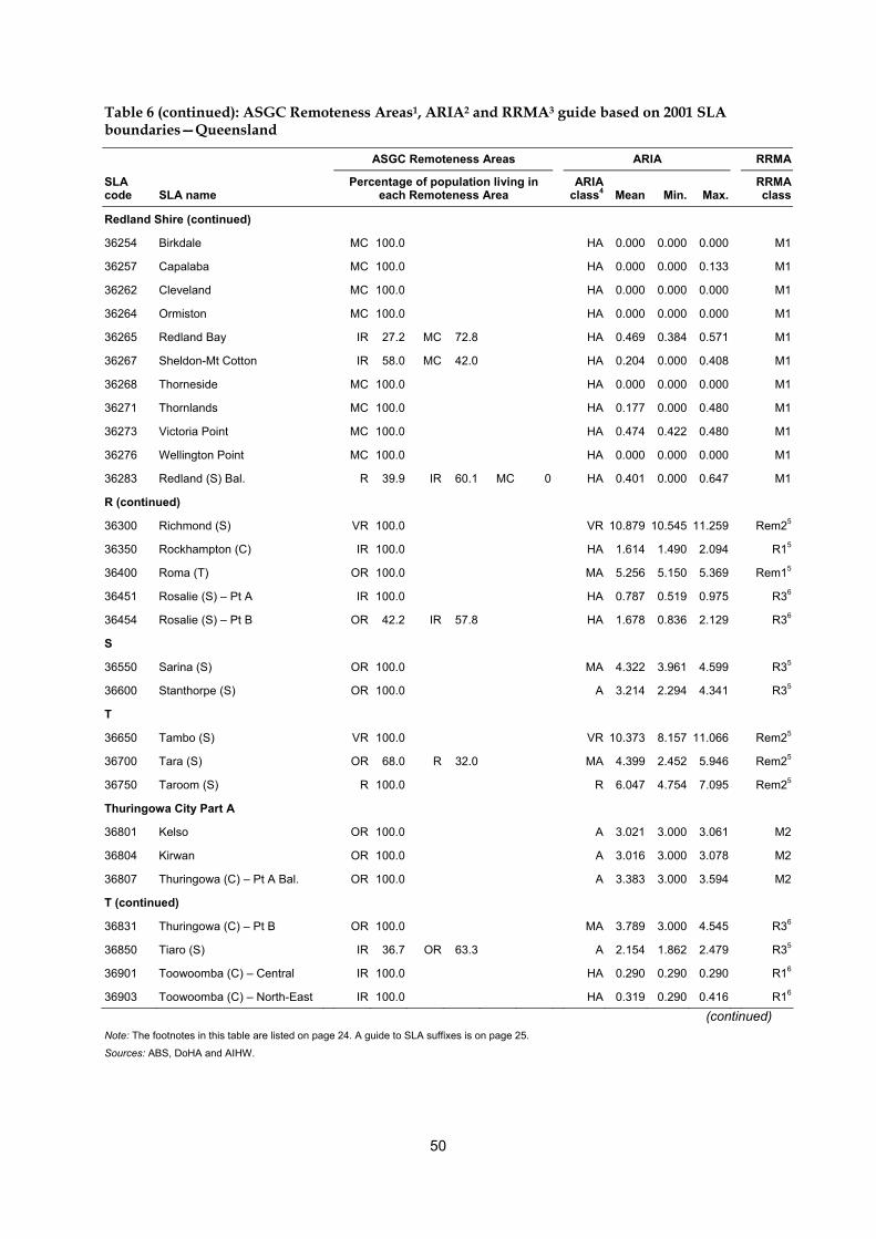
50
Table 6 (continued): ASGC Remoteness Areas1, ARIA2 and RRMA3 guide based on 2001 SLA boundaries—Queensland
ASGC Remoteness Areas ARIA RRMA
SLA code SLA name
Percentage of population living in each Remoteness Area
ARIA class4
Mean
Min. Max.
RRMA class
Redland Shire (continued)
36254 Birkdale MC 100.0 HA 0.000 0.000 0.000 M1
36257 Capalaba MC 100.0 HA 0.000 0.000 0.133 M1
36262 Cleveland MC 100.0 HA 0.000 0.000 0.000 M1
36264 Ormiston MC 100.0 HA 0.000 0.000 0.000 M1
36265 Redland Bay IR 27.2 MC 72.8 HA 0.469 0.384 0.571 M1
36267 Sheldon-Mt Cotton IR 58.0 MC 42.0 HA 0.204 0.000 0.408 M1
36268 Thorneside MC 100.0 HA 0.000 0.000 0.000 M1
36271 Thornlands MC 100.0 HA 0.177 0.000 0.480 M1
36273 Victoria Point MC 100.0 HA 0.474 0.422 0.480 M1
36276 Wellington Point MC 100.0 HA 0.000 0.000 0.000 M1
36283 Redland (S) Bal. R 39.9 IR 60.1 MC 0 HA 0.401 0.000 0.647 M1
R (continued)
36300 Richmond (S) VR 100.0 VR 10.879 10.545 11.259 Rem25
36350 Rockhampton (C) IR 100.0 HA 1.614 1.490 2.094 R15
36400 Roma (T) OR 100.0 MA 5.256 5.150 5.369 Rem15
36451 Rosalie (S) – Pt A IR 100.0 HA 0.787 0.519 0.975 R36
36454 Rosalie (S) – Pt B OR 42.2 IR 57.8 HA 1.678 0.836 2.129 R36
S
36550 Sarina (S) OR 100.0 MA 4.322 3.961 4.599 R35
36600 Stanthorpe (S) OR 100.0 A 3.214 2.294 4.341 R35
T
36650 Tambo (S) VR 100.0 VR 10.373 8.157 11.066 Rem25
36700 Tara (S) OR 68.0 R 32.0 MA 4.399 2.452 5.946 Rem25
36750 Taroom (S) R 100.0 R 6.047 4.754 7.095 Rem25
Thuringowa City Part A
36801 Kelso OR 100.0 A 3.021 3.000 3.061 M2
36804 Kirwan OR 100.0 A 3.016 3.000 3.078 M2
36807 Thuringowa (C) – Pt A Bal. OR 100.0 A 3.383 3.000 3.594 M2
T (continued)
36831 Thuringowa (C) – Pt B OR 100.0 MA 3.789 3.000 4.545 R36
36850 Tiaro (S) IR 36.7 OR 63.3 A 2.154 1.862 2.479 R35
36901 Toowoomba (C) – Central IR 100.0 HA 0.290 0.290 0.290 R16
36903 Toowoomba (C) – North-East IR 100.0 HA 0.319 0.290 0.416 R16
(continued) Note: The footnotes in this table are listed on page 24. A guide to SLA suffixes is on page 25.
Sources: ABS, DoHA and AIHW.
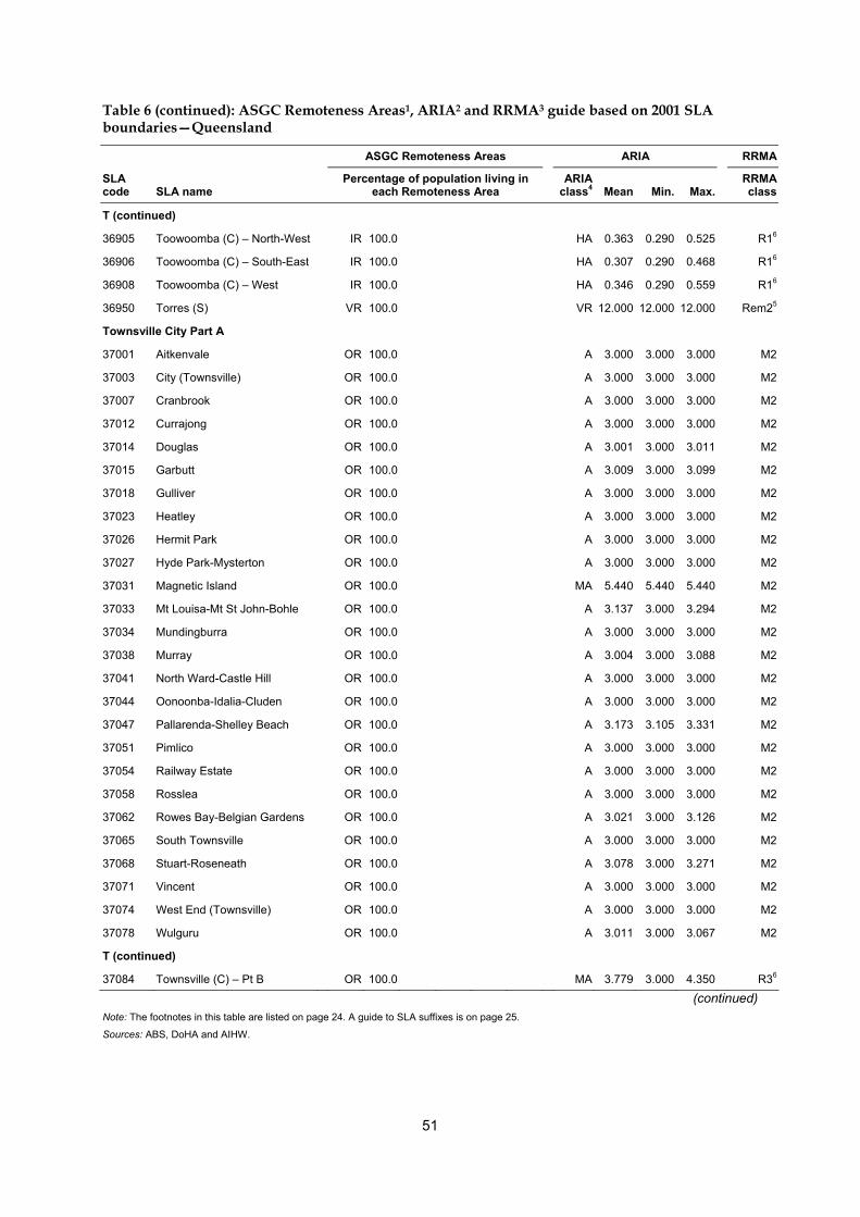
51
Table 6 (continued): ASGC Remoteness Areas1, ARIA2 and RRMA3 guide based on 2001 SLA boundaries—Queensland
ASGC Remoteness Areas ARIA RRMA
SLA code SLA name
Percentage of population living in each Remoteness Area
ARIA class4
Mean
Min. Max.
RRMA class
T (continued)
36905 Toowoomba (C) – North-West IR 100.0 HA 0.363 0.290 0.525 R16
36906 Toowoomba (C) – South-East IR 100.0 HA 0.307 0.290 0.468 R16
36908 Toowoomba (C) – West IR 100.0 HA 0.346 0.290 0.559 R16
36950 Torres (S) VR 100.0 VR 12.000 12.000 12.000 Rem25
Townsville City Part A
37001 Aitkenvale OR 100.0 A 3.000 3.000 3.000 M2
37003 City (Townsville) OR 100.0 A 3.000 3.000 3.000 M2
37007 Cranbrook OR 100.0 A 3.000 3.000 3.000 M2
37012 Currajong OR 100.0 A 3.000 3.000 3.000 M2
37014 Douglas OR 100.0 A 3.001 3.000 3.011 M2
37015 Garbutt OR 100.0 A 3.009 3.000 3.099 M2
37018 Gulliver OR 100.0 A 3.000 3.000 3.000 M2
37023 Heatley OR 100.0 A 3.000 3.000 3.000 M2
37026 Hermit Park OR 100.0 A 3.000 3.000 3.000 M2
37027 Hyde Park-Mysterton OR 100.0 A 3.000 3.000 3.000 M2
37031 Magnetic Island OR 100.0 MA 5.440 5.440 5.440 M2
37033 Mt Louisa-Mt St John-Bohle OR 100.0 A 3.137 3.000 3.294 M2
37034 Mundingburra OR 100.0 A 3.000 3.000 3.000 M2
37038 Murray OR 100.0 A 3.004 3.000 3.088 M2
37041 North Ward-Castle Hill OR 100.0 A 3.000 3.000 3.000 M2
37044 Oonoonba-Idalia-Cluden OR 100.0 A 3.000 3.000 3.000 M2
37047 Pallarenda-Shelley Beach OR 100.0 A 3.173 3.105 3.331 M2
37051 Pimlico OR 100.0 A 3.000 3.000 3.000 M2
37054 Railway Estate OR 100.0 A 3.000 3.000 3.000 M2
37058 Rosslea OR 100.0 A 3.000 3.000 3.000 M2
37062 Rowes Bay-Belgian Gardens OR 100.0 A 3.021 3.000 3.126 M2
37065 South Townsville OR 100.0 A 3.000 3.000 3.000 M2
37068 Stuart-Roseneath OR 100.0 A 3.078 3.000 3.271 M2
37071 Vincent OR 100.0 A 3.000 3.000 3.000 M2
37074 West End (Townsville) OR 100.0 A 3.000 3.000 3.000 M2
37078 Wulguru OR 100.0 A 3.011 3.000 3.067 M2
T (continued)
37084 Townsville (C) – Pt B OR 100.0 MA 3.779 3.000 4.350 R36
(continued) Note: The footnotes in this table are listed on page 24. A guide to SLA suffixes is on page 25.
Sources: ABS, DoHA and AIHW.
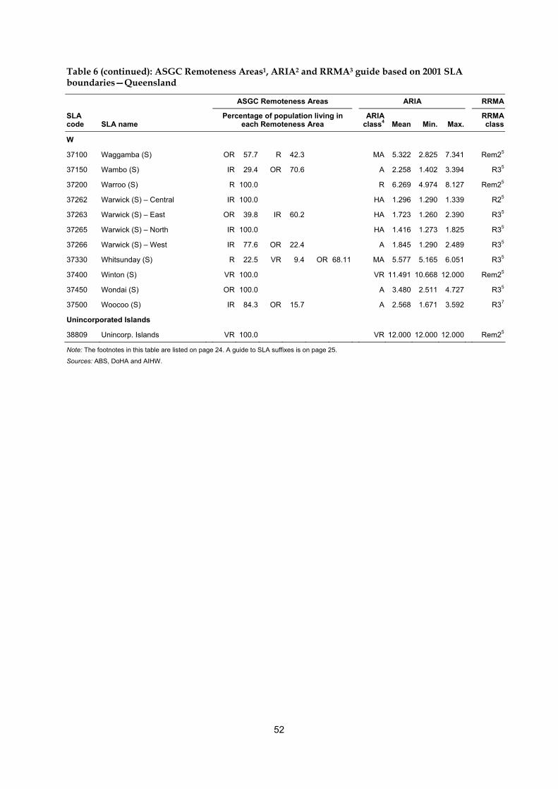
52
Table 6 (continued): ASGC Remoteness Areas1, ARIA2 and RRMA3 guide based on 2001 SLA boundaries—Queensland
ASGC Remoteness Areas ARIA RRMA
SLA code SLA name
Percentage of population living in each Remoteness Area
ARIA class4
Mean
Min. Max.
RRMA class
W
37100 Waggamba (S) OR 57.7 R 42.3 MA 5.322 2.825 7.341 Rem25
37150 Wambo (S) IR 29.4 OR 70.6 A 2.258 1.402 3.394 R35
37200 Warroo (S) R 100.0 R 6.269 4.974 8.127 Rem25
37262 Warwick (S) – Central IR 100.0 HA 1.296 1.290 1.339 R25
37263 Warwick (S) – East OR 39.8 IR 60.2 HA 1.723 1.260 2.390 R35
37265 Warwick (S) – North IR 100.0 HA 1.416 1.273 1.825 R35
37266 Warwick (S) – West IR 77.6 OR 22.4 A 1.845 1.290 2.489 R35
37330 Whitsunday (S) R 22.5 VR 9.4 OR 68.11 MA 5.577 5.165 6.051 R35
37400 Winton (S) VR 100.0 VR 11.491 10.668 12.000 Rem25
37450 Wondai (S) OR 100.0 A 3.480 2.511 4.727 R35
37500 Woocoo (S) IR 84.3 OR 15.7 A 2.568 1.671 3.592 R37
Unincorporated Islands
38809 Unincorp. Islands VR 100.0 VR 12.000 12.000 12.000 Rem25
Note: The footnotes in this table are listed on page 24. A guide to SLA suffixes is on page 25.
Sources: ABS, DoHA and AIHW.
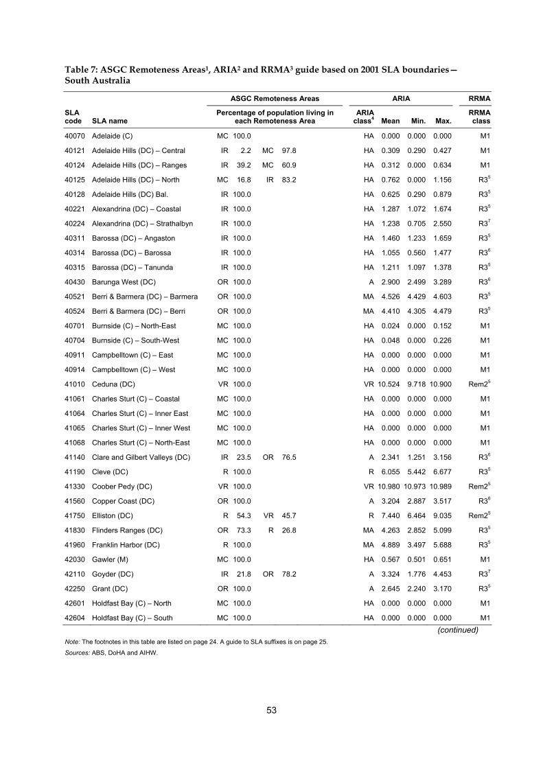
53
Table 7: ASGC Remoteness Areas1, ARIA2 and RRMA3 guide based on 2001 SLA boundaries—South Australia
ASGC Remoteness Areas ARIA RRMA
SLA code SLA name
Percentage of population living in each Remoteness Area
ARIA class4
Mean
Min. Max.
RRMA class
40070 Adelaide (C) MC 100.0 HA 0.000 0.000 0.000 M1
40121 Adelaide Hills (DC) – Central IR 2.2 MC 97.8 HA 0.309 0.290 0.427 M1
40124 Adelaide Hills (DC) – Ranges IR 39.2 MC 60.9 HA 0.312 0.000 0.634 M1
40125 Adelaide Hills (DC) – North MC 16.8 IR 83.2 HA 0.762 0.000 1.156 R35
40128 Adelaide Hills (DC) Bal. IR 100.0 HA 0.625 0.290 0.879 R35
40221 Alexandrina (DC) – Coastal IR 100.0 HA 1.287 1.072 1.674 R35
40224 Alexandrina (DC) – Strathalbyn IR 100.0 HA 1.238 0.705 2.550 R37
40311 Barossa (DC) – Angaston IR 100.0 HA 1.460 1.233 1.659 R35
40314 Barossa (DC) – Barossa IR 100.0 HA 1.055 0.560 1.477 R36
40315 Barossa (DC) – Tanunda IR 100.0 HA 1.211 1.097 1.378 R35
40430 Barunga West (DC) OR 100.0 A 2.900 2.499 3.289 R36
40521 Berri & Barmera (DC) – Barmera OR 100.0 MA 4.526 4.429 4.603 R35
40524 Berri & Barmera (DC) – Berri OR 100.0 MA 4.410 4.305 4.479 R35
40701 Burnside (C) – North-East MC 100.0 HA 0.024 0.000 0.152 M1
40704 Burnside (C) – South-West MC 100.0 HA 0.048 0.000 0.226 M1
40911 Campbelltown (C) – East MC 100.0 HA 0.000 0.000 0.000 M1
40914 Campbelltown (C) – West MC 100.0 HA 0.000 0.000 0.000 M1
41010 Ceduna (DC) VR 100.0 VR 10.524 9.718 10.900 Rem25
41061 Charles Sturt (C) – Coastal MC 100.0 HA 0.000 0.000 0.000 M1
41064 Charles Sturt (C) – Inner East MC 100.0 HA 0.000 0.000 0.000 M1
41065 Charles Sturt (C) – Inner West MC 100.0 HA 0.000 0.000 0.000 M1
41068 Charles Sturt (C) – North-East MC 100.0 HA 0.000 0.000 0.000 M1
41140 Clare and Gilbert Valleys (DC) IR 23.5 OR 76.5 A 2.341 1.251 3.156 R36
41190 Cleve (DC) R 100.0 R 6.055 5.442 6.677 R35
41330 Coober Pedy (DC) VR 100.0 VR 10.980 10.973 10.989 Rem25
41560 Copper Coast (DC) OR 100.0 A 3.204 2.887 3.517 R36
41750 Elliston (DC) R 54.3 VR 45.7 R 7.440 6.464 9.035 Rem25
41830 Flinders Ranges (DC) OR 73.3 R 26.8 MA 4.263 2.852 5.099 R35
41960 Franklin Harbor (DC) R 100.0 MA 4.889 3.497 5.688 R35
42030 Gawler (M) MC 100.0 HA 0.567 0.501 0.651 M1
42110 Goyder (DC) IR 21.8 OR 78.2 A 3.324 1.776 4.453 R37
42250 Grant (DC) OR 100.0 A 2.645 2.240 3.170 R35
42601 Holdfast Bay (C) – North MC 100.0 HA 0.000 0.000 0.000 M1
42604 Holdfast Bay (C) – South MC 100.0 HA 0.000 0.000 0.000 M1
(continued) Note: The footnotes in this table are listed on page 24. A guide to SLA suffixes is on page 25.
Sources: ABS, DoHA and AIHW.

54
Table 7 (continued): ASGC Remoteness Areas1, ARIA2 and RRMA3 guide based on 2001 SLA boundaries—South Australia
ASGC Remoteness Areas ARIA RRMA
SLA code SLA name
Percentage of population living in each Remoteness Area
ARIA class4
Mean
Min. Max.
RRMA class
42750 Kangaroo Island (DC) R 100.0 R 8.080 8.080 8.080 Rem26
43080 Karoonda East Murray (DC) OR 100.0 A 3.032 1.991 4.119 R35
43220 Kimba (DC) R 100.0 MA 5.772 4.442 6.712 R35
43360 Lacepede (DC) OR 89.0 R 11.0 MA 4.409 3.820 4.760 R35
43570 Le Hunte (DC) R 17.9 VR 82.1 R 7.899 6.274 9.272 Rem25
43650 Light (DC) MC 3.8 IR 96.2 HA 1.257 0.560 1.931 R36
43710 Lower Eyre Peninsula (DC) R 100.0 R 6.601 5.981 7.230 R35
43791 Loxton Waikerie (DC) – East OR 100.0 MA 4.313 3.461 4.880 R35
43794 Loxton Waikerie (DC) – West OR 100.0 MA 3.630 2.786 4.472 R35
43920 Mallala (DC) IR 100.0 HA 1.156 0.587 1.641 R35
44061 Marion (C) – Central MC 100.0 HA 0.000 0.000 0.000 M1
44064 Marion (C) – North MC 100.0 HA 0.000 0.000 0.000 M1
44065 Marion (C) – South MC 100.0 HA 0.000 0.000 0.000 M1
44210 Mid Murray (DC) IR 65.9 OR 34.1 A 2.447 0.886 3.968 R36
44341 Mitcham (C) – Hills MC 100.0 HA 0.081 0.000 0.254 M1
44344 Mitcham (C) – North-East MC 100.0 HA 0.000 0.000 0.000 M1
44345 Mitcham (C) – West MC 100.0 HA 0.000 0.000 0.000 M1
44551 Mount Barker (DC) – Central IR 100.0 HA 0.502 0.448 0.610 R36
44554 Mount Barker (DC) Bal. IR 100.0 HA 0.706 0.420 1.004 R36
44620 Mount Gambier (C) IR 100.0 A 2.248 2.240 2.326 R26
44830 Mount Remarkable (DC) OR 100.0 A 3.251 2.699 3.985 R35
45040 Murray Bridge (RC) IR 100.0 HA 1.419 0.891 2.493 R25
45090 Naracoorte and Lucindale (DC) OR 100.0 MA 3.905 3.044 4.518 R36
45120 Northern Areas (DC) OR 100.0 A 3.275 2.722 3.894 R36
45291 Norw. P'ham St Ptrs (C) – East MC 100.0 HA 0.000 0.000 0.000 M1
45294 Norw. P'ham St Ptrs (C) – West MC 100.0 HA 0.000 0.000 0.000 M1
45341 Onkaparinga (C) – Hackham MC 100.0 HA 0.375 0.000 0.675 M1
45342 Onkaparinga (C) – Hills IR 62.9 MC 37.1 HA 0.796 0.000 1.122 M1
45343 Onkaparinga (C) – Morphett MC 100.0 HA 0.000 0.000 0.000 M1
45344 Onkaparinga (C) – North Coast MC 100.0 HA 0.000 0.000 0.000 M1
45345 Onkaparinga (C) – Reservoir MC 100.0 HA 0.000 0.000 0.000 M1
45346 Onkaparinga (C) – South Coast IR 34.9 MC 65.1 HA 0.725 0.000 1.121 M1
45347 Onkaparinga (C) – Woodcroft MC 100.0 HA 0.000 0.000 0.512 M1
45400 Orroroo/Carrieton (DC) OR 85.9 R 14.1 MA 4.145 3.456 4.730 R36
45540 Peterborough (DC) OR 100.0 MA 4.552 3.718 5.249 R36
(continued) Note: The footnotes in this table are listed on page 24. A guide to SLA suffixes is on page 25.
Sources: ABS, DoHA and AIHW.
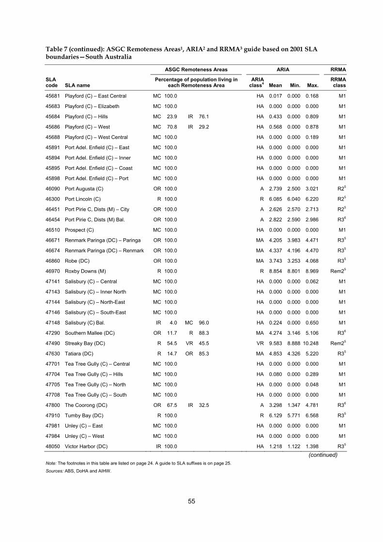
55
Table 7 (continued): ASGC Remoteness Areas1, ARIA2 and RRMA3 guide based on 2001 SLA boundaries—South Australia
ASGC Remoteness Areas ARIA RRMA
SLA code SLA name
Percentage of population living in each Remoteness Area
ARIA class4
Mean
Min. Max.
RRMA class
45681 Playford (C) – East Central MC 100.0 HA 0.017 0.000 0.168 M1
45683 Playford (C) – Elizabeth MC 100.0 HA 0.000 0.000 0.000 M1
45684 Playford (C) – Hills MC 23.9 IR 76.1 HA 0.433 0.000 0.809 M1
45686 Playford (C) – West MC 70.8 IR 29.2 HA 0.568 0.000 0.878 M1
45688 Playford (C) – West Central MC 100.0 HA 0.000 0.000 0.189 M1
45891 Port Adel. Enfield (C) – East MC 100.0 HA 0.000 0.000 0.000 M1
45894 Port Adel. Enfield (C) – Inner MC 100.0 HA 0.000 0.000 0.000 M1
45895 Port Adel. Enfield (C) – Coast MC 100.0 HA 0.000 0.000 0.000 M1
45898 Port Adel. Enfield (C) – Port MC 100.0 HA 0.000 0.000 0.000 M1
46090 Port Augusta (C) OR 100.0 A 2.739 2.500 3.021 R25
46300 Port Lincoln (C) R 100.0 R 6.085 6.040 6.220 R25
46451 Port Pirie C, Dists (M) – City OR 100.0 A 2.626 2.570 2.713 R25
46454 Port Pirie C, Dists (M) Bal. OR 100.0 A 2.822 2.590 2.986 R36
46510 Prospect (C) MC 100.0 HA 0.000 0.000 0.000 M1
46671 Renmark Paringa (DC) – Paringa OR 100.0 MA 4.205 3.983 4.471 R35
46674 Renmark Paringa (DC) – Renmark OR 100.0 MA 4.337 4.196 4.470 R35
46860 Robe (DC) OR 100.0 MA 3.743 3.253 4.068 R35
46970 Roxby Downs (M) R 100.0 R 8.854 8.801 8.969 Rem25
47141 Salisbury (C) – Central MC 100.0 HA 0.000 0.000 0.062 M1
47143 Salisbury (C) – Inner North MC 100.0 HA 0.000 0.000 0.000 M1
47144 Salisbury (C) – North-East MC 100.0 HA 0.000 0.000 0.000 M1
47146 Salisbury (C) – South-East MC 100.0 HA 0.000 0.000 0.000 M1
47148 Salisbury (C) Bal. IR 4.0 MC 96.0 HA 0.224 0.000 0.650 M1
47290 Southern Mallee (DC) OR 11.7 R 88.3 MA 4.274 3.146 5.106 R36
47490 Streaky Bay (DC) R 54.5 VR 45.5 VR 9.583 8.888 10.248 Rem25
47630 Tatiara (DC) R 14.7 OR 85.3 MA 4.853 4.326 5.220 R35
47701 Tea Tree Gully (C) – Central MC 100.0 HA 0.000 0.000 0.000 M1
47704 Tea Tree Gully (C) – Hills MC 100.0 HA 0.080 0.000 0.289 M1
47705 Tea Tree Gully (C) – North MC 100.0 HA 0.000 0.000 0.048 M1
47708 Tea Tree Gully (C) – South MC 100.0 HA 0.000 0.000 0.000 M1
47800 The Coorong (DC) OR 67.5 IR 32.5 A 3.298 1.347 4.781 R36
47910 Tumby Bay (DC) R 100.0 R 6.129 5.771 6.568 R35
47981 Unley (C) – East MC 100.0 HA 0.000 0.000 0.000 M1
47984 Unley (C) – West MC 100.0 HA 0.000 0.000 0.000 M1
48050 Victor Harbor (DC) IR 100.0 HA 1.218 1.122 1.398 R35
(continued) Note: The footnotes in this table are listed on page 24. A guide to SLA suffixes is on page 25.
Sources: ABS, DoHA and AIHW.
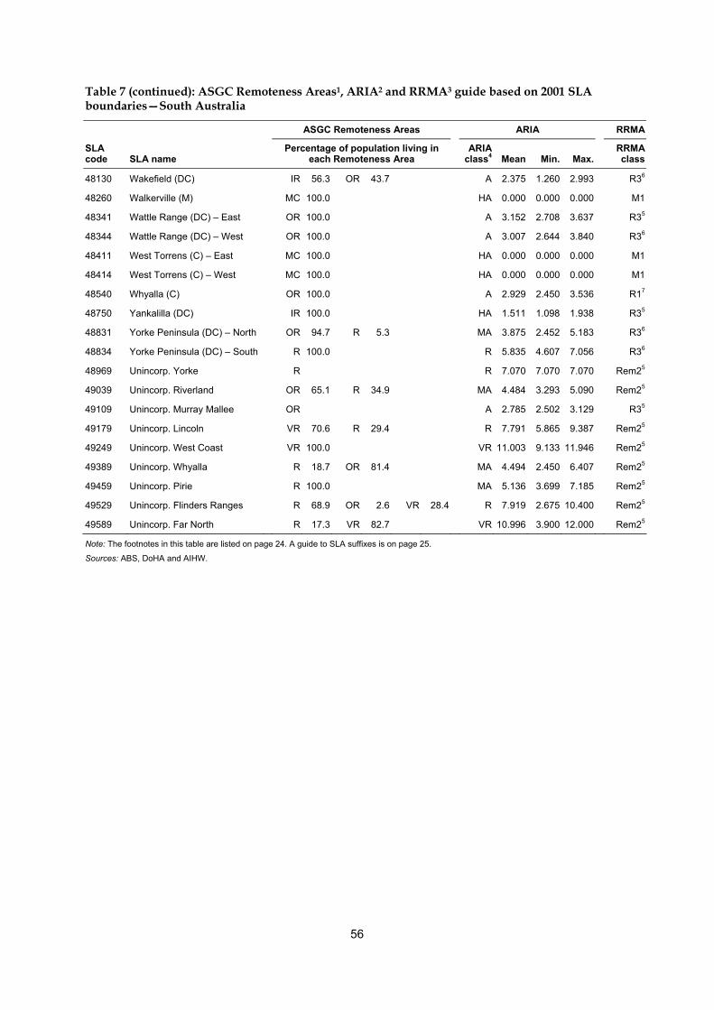
56
Table 7 (continued): ASGC Remoteness Areas1, ARIA2 and RRMA3 guide based on 2001 SLA boundaries—South Australia
ASGC Remoteness Areas ARIA RRMA
SLA code SLA name
Percentage of population living in each Remoteness Area
ARIA class4
Mean
Min. Max.
RRMA class
48130 Wakefield (DC) IR 56.3 OR 43.7 A 2.375 1.260 2.993 R36
48260 Walkerville (M) MC 100.0 HA 0.000 0.000 0.000 M1
48341 Wattle Range (DC) – East OR 100.0 A 3.152 2.708 3.637 R35
48344 Wattle Range (DC) – West OR 100.0 A 3.007 2.644 3.840 R36
48411 West Torrens (C) – East MC 100.0 HA 0.000 0.000 0.000 M1
48414 West Torrens (C) – West MC 100.0 HA 0.000 0.000 0.000 M1
48540 Whyalla (C) OR 100.0 A 2.929 2.450 3.536 R17
48750 Yankalilla (DC) IR 100.0 HA 1.511 1.098 1.938 R35
48831 Yorke Peninsula (DC) – North OR 94.7 R 5.3 MA 3.875 2.452 5.183 R36
48834 Yorke Peninsula (DC) – South R 100.0 R 5.835 4.607 7.056 R36
48969 Unincorp. Yorke R R 7.070 7.070 7.070 Rem25
49039 Unincorp. Riverland OR 65.1 R 34.9 MA 4.484 3.293 5.090 Rem25
49109 Unincorp. Murray Mallee OR A 2.785 2.502 3.129 R35
49179 Unincorp. Lincoln VR 70.6 R 29.4 R 7.791 5.865 9.387 Rem25
49249 Unincorp. West Coast VR 100.0 VR 11.003 9.133 11.946 Rem25
49389 Unincorp. Whyalla R 18.7 OR 81.4 MA 4.494 2.450 6.407 Rem25
49459 Unincorp. Pirie R 100.0 MA 5.136 3.699 7.185 Rem25
49529 Unincorp. Flinders Ranges R 68.9 OR 2.6 VR 28.4 R 7.919 2.675 10.400 Rem25
49589 Unincorp. Far North R 17.3 VR 82.7 VR 10.996 3.900 12.000 Rem25
Note: The footnotes in this table are listed on page 24. A guide to SLA suffixes is on page 25.
Sources: ABS, DoHA and AIHW.
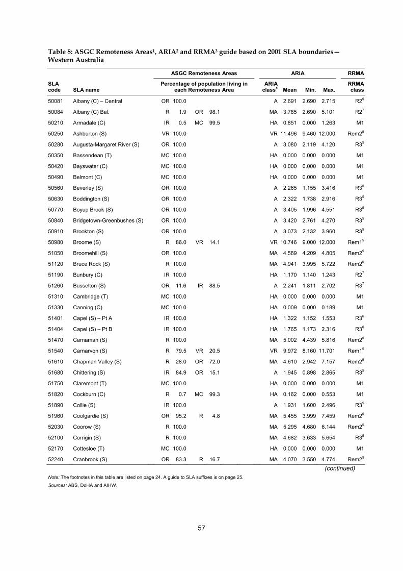
57
Table 8: ASGC Remoteness Areas1, ARIA2 and RRMA3 guide based on 2001 SLA boundaries—Western Australia
ASGC Remoteness Areas ARIA RRMA
SLA code SLA name
Percentage of population living in each Remoteness Area
ARIA class4
Mean
Min. Max.
RRMA class
50081 Albany (C) – Central OR 100.0 A 2.691 2.690 2.715 R25
50084 Albany (C) Bal. R 1.9 OR 98.1 MA 3.785 2.690 5.101 R27
50210 Armadale (C) IR 0.5 MC 99.5 HA 0.851 0.000 1.263 M1
50250 Ashburton (S) VR 100.0 VR 11.496 9.460 12.000 Rem25
50280 Augusta-Margaret River (S) OR 100.0 A 3.080 2.119 4.120 R35
50350 Bassendean (T) MC 100.0 HA 0.000 0.000 0.000 M1
50420 Bayswater (C) MC 100.0 HA 0.000 0.000 0.000 M1
50490 Belmont (C) MC 100.0 HA 0.000 0.000 0.000 M1
50560 Beverley (S) OR 100.0 A 2.265 1.155 3.416 R35
50630 Boddington (S) OR 100.0 A 2.322 1.738 2.916 R35
50770 Boyup Brook (S) OR 100.0 A 3.405 1.996 4.551 R35
50840 Bridgetown-Greenbushes (S) OR 100.0 A 3.420 2.761 4.270 R35
50910 Brookton (S) OR 100.0 A 3.073 2.132 3.960 R35
50980 Broome (S) R 86.0 VR 14.1 VR 10.746 9.000 12.000 Rem15
51050 Broomehill (S) OR 100.0 MA 4.589 4.209 4.805 Rem25
51120 Bruce Rock (S) R 100.0 MA 4.941 3.995 5.722 Rem25
51190 Bunbury (C) IR 100.0 HA 1.170 1.140 1.243 R27
51260 Busselton (S) OR 11.6 IR 88.5 A 2.241 1.811 2.702 R37
51310 Cambridge (T) MC 100.0 HA 0.000 0.000 0.000 M1
51330 Canning (C) MC 100.0 HA 0.009 0.000 0.189 M1
51401 Capel (S) – Pt A IR 100.0 HA 1.322 1.152 1.553 R36
51404 Capel (S) – Pt B IR 100.0 HA 1.765 1.173 2.316 R36
51470 Carnamah (S) R 100.0 MA 5.002 4.439 5.816 Rem25
51540 Carnarvon (S) R 79.5 VR 20.5 VR 9.972 8.160 11.701 Rem15
51610 Chapman Valley (S) R 28.0 OR 72.0 MA 4.610 2.942 7.157 Rem25
51680 Chittering (S) IR 84.9 OR 15.1 A 1.945 0.898 2.865 R35
51750 Claremont (T) MC 100.0 HA 0.000 0.000 0.000 M1
51820 Cockburn (C) R 0.7 MC 99.3 HA 0.162 0.000 0.553 M1
51890 Collie (S) IR 100.0 A 1.931 1.600 2.496 R35
51960 Coolgardie (S) OR 95.2 R 4.8 MA 5.455 3.999 7.459 Rem25
52030 Coorow (S) R 100.0 MA 5.295 4.680 6.144 Rem25
52100 Corrigin (S) R 100.0 MA 4.682 3.633 5.654 R35
52170 Cottesloe (T) MC 100.0 HA 0.000 0.000 0.000 M1
52240 Cranbrook (S) OR 83.3 R 16.7 MA 4.070 3.550 4.774 Rem25
(continued) Note: The footnotes in this table are listed on page 24. A guide to SLA suffixes is on page 25.
Sources: ABS, DoHA and AIHW.
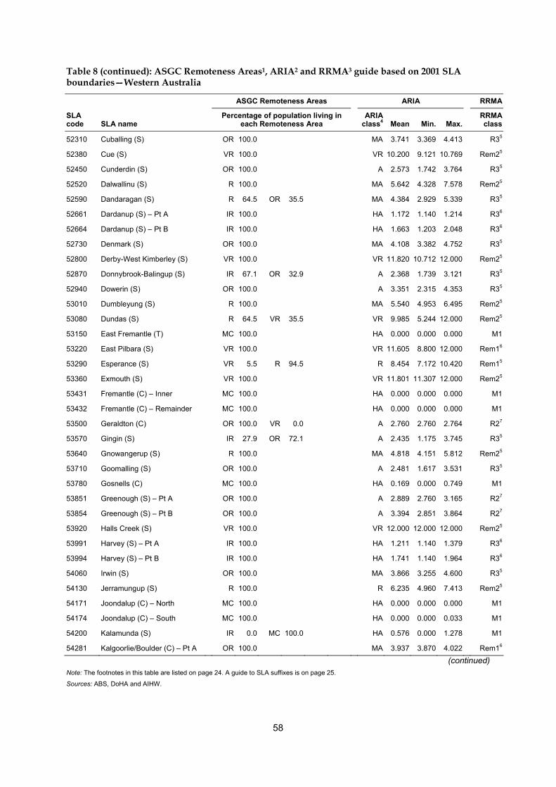
58
Table 8 (continued): ASGC Remoteness Areas1, ARIA2 and RRMA3 guide based on 2001 SLA boundaries—Western Australia
ASGC Remoteness Areas ARIA RRMA
SLA code SLA name
Percentage of population living in each Remoteness Area
ARIA class4
Mean
Min. Max.
RRMA class
52310 Cuballing (S) OR 100.0 MA 3.741 3.369 4.413 R35
52380 Cue (S) VR 100.0 VR 10.200 9.121 10.769 Rem25
52450 Cunderdin (S) OR 100.0 A 2.573 1.742 3.764 R35
52520 Dalwallinu (S) R 100.0 MA 5.642 4.328 7.578 Rem25
52590 Dandaragan (S) R 64.5 OR 35.5 MA 4.384 2.929 5.339 R35
52661 Dardanup (S) – Pt A IR 100.0 HA 1.172 1.140 1.214 R36
52664 Dardanup (S) – Pt B IR 100.0 HA 1.663 1.203 2.048 R36
52730 Denmark (S) OR 100.0 MA 4.108 3.382 4.752 R35
52800 Derby-West Kimberley (S) VR 100.0 VR 11.820 10.712 12.000 Rem25
52870 Donnybrook-Balingup (S) IR 67.1 OR 32.9 A 2.368 1.739 3.121 R35
52940 Dowerin (S) OR 100.0 A 3.351 2.315 4.353 R35
53010 Dumbleyung (S) R 100.0 MA 5.540 4.953 6.495 Rem25
53080 Dundas (S) R 64.5 VR 35.5 VR 9.985 5.244 12.000 Rem25
53150 East Fremantle (T) MC 100.0 HA 0.000 0.000 0.000 M1
53220 East Pilbara (S) VR 100.0 VR 11.605 8.800 12.000 Rem16
53290 Esperance (S) VR 5.5 R 94.5 R 8.454 7.172 10.420 Rem15
53360 Exmouth (S) VR 100.0 VR 11.801 11.307 12.000 Rem25
53431 Fremantle (C) – Inner MC 100.0 HA 0.000 0.000 0.000 M1
53432 Fremantle (C) – Remainder MC 100.0 HA 0.000 0.000 0.000 M1
53500 Geraldton (C) OR 100.0 VR 0.0 A 2.760 2.760 2.764 R27
53570 Gingin (S) IR 27.9 OR 72.1 A 2.435 1.175 3.745 R35
53640 Gnowangerup (S) R 100.0 MA 4.818 4.151 5.812 Rem25
53710 Goomalling (S) OR 100.0 A 2.481 1.617 3.531 R35
53780 Gosnells (C) MC 100.0 HA 0.169 0.000 0.749 M1
53851 Greenough (S) – Pt A OR 100.0 A 2.889 2.760 3.165 R27
53854 Greenough (S) – Pt B OR 100.0 A 3.394 2.851 3.864 R27
53920 Halls Creek (S) VR 100.0 VR 12.000 12.000 12.000 Rem25
53991 Harvey (S) – Pt A IR 100.0 HA 1.211 1.140 1.379 R36
53994 Harvey (S) – Pt B IR 100.0 HA 1.741 1.140 1.964 R36
54060 Irwin (S) OR 100.0 MA 3.866 3.255 4.600 R35
54130 Jerramungup (S) R 100.0 R 6.235 4.960 7.413 Rem25
54171 Joondalup (C) – North MC 100.0 HA 0.000 0.000 0.000 M1
54174 Joondalup (C) – South MC 100.0 HA 0.000 0.000 0.033 M1
54200 Kalamunda (S) IR 0.0 MC 100.0 HA 0.576 0.000 1.278 M1
54281 Kalgoorlie/Boulder (C) – Pt A OR 100.0 MA 3.937 3.870 4.022 Rem16
(continued) Note: The footnotes in this table are listed on page 24. A guide to SLA suffixes is on page 25.
Sources: ABS, DoHA and AIHW.

59
Table 8 (continued): ASGC Remoteness Areas1, ARIA2 and RRMA3 guide based on 2001 SLA boundaries—Western Australia
ASGC Remoteness Areas ARIA RRMA
SLA code SLA name
Percentage of population living in each Remoteness Area
ARIA class4
Mean
Min. Max.
RRMA class
54284 Kalgoorlie/Boulder (C) – Pt B VR 55.1 OR 0.0 R 44.9 VR 9.832 3.924 12.000 Rem17
54340 Katanning (S) R 3.9 OR 96.1 MA 4.837 4.426 5.488 R35
54410 Kellerberrin (S) OR 100.0 MA 4.323 3.615 5.418 R35
54480 Kent (S) R 100.0 R 6.062 4.828 7.462 Rem25
54550 Kojonup (S) OR 100.0 MA 4.092 3.439 4.475 R35
54620 Kondinin (S) VR 28.8 R 71.2 R 7.341 5.282 7.977 Rem25
54690 Koorda (S) R 100.0 MA 5.071 4.015 6.262 Rem25
54760 Kulin (S) VR 16.9 R 83.1 R 6.713 4.888 8.009 Rem25
54830 Kwinana (T) IR 11.5 MC 88.5 HA 0.371 0.290 0.535 M1
54900 Lake Grace (S) VR 25.4 R 74.6 R 7.421 5.849 8.120 Rem25
54970 Laverton (S) VR 100.0 VR 11.401 9.136 12.000 Rem25
55040 Leonora (S) R 36.5 VR 63.5 VR 10.145 8.488 11.235 Rem25
55110 Mandurah (C) MC 0.7 IR 99.3 HA 0.753 0.470 1.472 R27
55180 Manjimup (S) R 15.7 OR 84.3 MA 4.796 3.649 5.420 R35
55250 Meekatharra (S) VR 100.0 VR 10.913 8.861 11.840 Rem25
55320 Melville (C) MC 100.0 HA 0.001 0.000 0.074 M1
55390 Menzies (S) R 50.0 VR 50.0 VR 9.785 5.047 11.976 Rem25
55460 Merredin (S) R 14.8 OR 85.2 MA 5.624 4.553 6.736 Rem25
55530 Mingenew (S) OR 56.2 R 43.9 MA 4.461 3.920 5.371 Rem25
55600 Moora (S) OR 100.0 MA 4.351 3.051 5.449 R35
55670 Morawa (S) R 100.0 MA 5.486 4.750 6.704 Rem25
55740 Mosman Park (T) MC 100.0 HA 0.000 0.000 0.000 M1
55810 Mount Magnet (S) VR 100.0 VR 9.159 8.584 10.115 Rem25
55880 Mount Marshall (S) R 89.4 VR 10.6 R 6.976 4.544 8.489 Rem25
55950 Mukinbudin (S) R 100.0 R 6.817 5.666 7.389 Rem25
56020 Mullewa (S) R 100.0 MA 5.739 3.653 8.047 Rem25
56090 Mundaring (S) IR 25.8 MC 74.2 HA 1.002 0.000 1.289 M1
56160 Murchison (S) VR 100.0 VR 9.793 5.283 10.920 Rem25
56230 Murray (S) IR 100.0 HA 1.242 0.470 1.934 R35
56300 Nannup (S) OR 100.0 A 3.432 2.428 4.642 R35
56370 Narembeen (S) R 100.0 R 6.335 5.349 7.490 Rem25
56440 Narrogin (T) OR 100.0 MA 3.757 3.751 3.766 R35
56510 Narrogin (S) OR 100.0 MA 3.903 3.191 4.674 R35
56580 Nedlands (C) MC 100.0 HA 0.000 0.000 0.000 M1
56620 Ngaanyatjarraku (S) VR 100.0 VR 12.000 11.850 12.000 Rem26
(continued) Note: The footnotes in this table are listed on page 24. A guide to SLA suffixes is on page 25.
Sources: ABS, DoHA and AIHW.
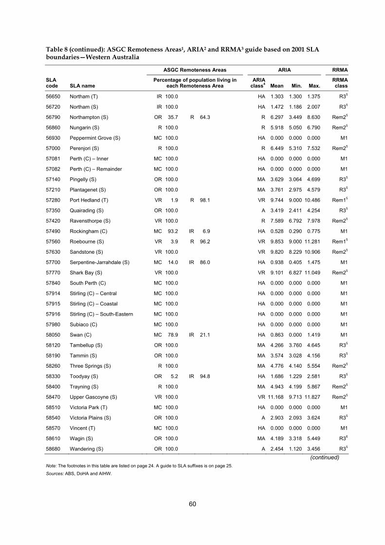
60
Table 8 (continued): ASGC Remoteness Areas1, ARIA2 and RRMA3 guide based on 2001 SLA boundaries—Western Australia
ASGC Remoteness Areas ARIA RRMA
SLA code SLA name
Percentage of population living in each Remoteness Area
ARIA class4
Mean
Min. Max.
RRMA class
56650 Northam (T) IR 100.0 HA 1.303 1.300 1.375 R35
56720 Northam (S) IR 100.0 HA 1.472 1.186 2.007 R35
56790 Northampton (S) OR 35.7 R 64.3 R 6.297 3.449 8.630 Rem25
56860 Nungarin (S) R 100.0 R 5.918 5.050 6.790 Rem25
56930 Peppermint Grove (S) MC 100.0 HA 0.000 0.000 0.000 M1
57000 Perenjori (S) R 100.0 R 6.449 5.310 7.532 Rem25
57081 Perth (C) – Inner MC 100.0 HA 0.000 0.000 0.000 M1
57082 Perth (C) – Remainder MC 100.0 HA 0.000 0.000 0.000 M1
57140 Pingelly (S) OR 100.0 MA 3.629 3.064 4.699 R35
57210 Plantagenet (S) OR 100.0 MA 3.761 2.975 4.579 R35
57280 Port Hedland (T) VR 1.9 R 98.1 VR 9.744 9.000 10.486 Rem15
57350 Quairading (S) OR 100.0 A 3.419 2.411 4.254 R35
57420 Ravensthorpe (S) VR 100.0 R 7.589 6.792 7.978 Rem25
57490 Rockingham (C) MC 93.2 IR 6.9 HA 0.528 0.290 0.775 M1
57560 Roebourne (S) VR 3.9 R 96.2 VR 9.853 9.000 11.281 Rem15
57630 Sandstone (S) VR 100.0 VR 9.820 8.229 10.906 Rem25
57700 Serpentine-Jarrahdale (S) MC 14.0 IR 86.0 HA 0.938 0.405 1.475 M1
57770 Shark Bay (S) VR 100.0 VR 9.101 6.827 11.049 Rem25
57840 South Perth (C) MC 100.0 HA 0.000 0.000 0.000 M1
57914 Stirling (C) – Central MC 100.0 HA 0.000 0.000 0.000 M1
57915 Stirling (C) – Coastal MC 100.0 HA 0.000 0.000 0.000 M1
57916 Stirling (C) – South-Eastern MC 100.0 HA 0.000 0.000 0.000 M1
57980 Subiaco (C) MC 100.0 HA 0.000 0.000 0.000 M1
58050 Swan (C) MC 78.9 IR 21.1 HA 0.863 0.000 1.419 M1
58120 Tambellup (S) OR 100.0 MA 4.266 3.760 4.645 R35
58190 Tammin (S) OR 100.0 MA 3.574 3.028 4.156 R35
58260 Three Springs (S) R 100.0 MA 4.776 4.140 5.554 Rem25
58330 Toodyay (S) OR 5.2 IR 94.8 HA 1.686 1.229 2.581 R35
58400 Trayning (S) R 100.0 MA 4.943 4.199 5.867 Rem25
58470 Upper Gascoyne (S) VR 100.0 VR 11.168 9.713 11.827 Rem25
58510 Victoria Park (T) MC 100.0 HA 0.000 0.000 0.000 M1
58540 Victoria Plains (S) OR 100.0 A 2.903 2.093 3.624 R35
58570 Vincent (T) MC 100.0 HA 0.000 0.000 0.000 M1
58610 Wagin (S) OR 100.0 MA 4.189 3.318 5.449 R36
58680 Wandering (S) OR 100.0 A 2.454 1.120 3.456 R35
(continued) Note: The footnotes in this table are listed on page 24. A guide to SLA suffixes is on page 25.
Sources: ABS, DoHA and AIHW.
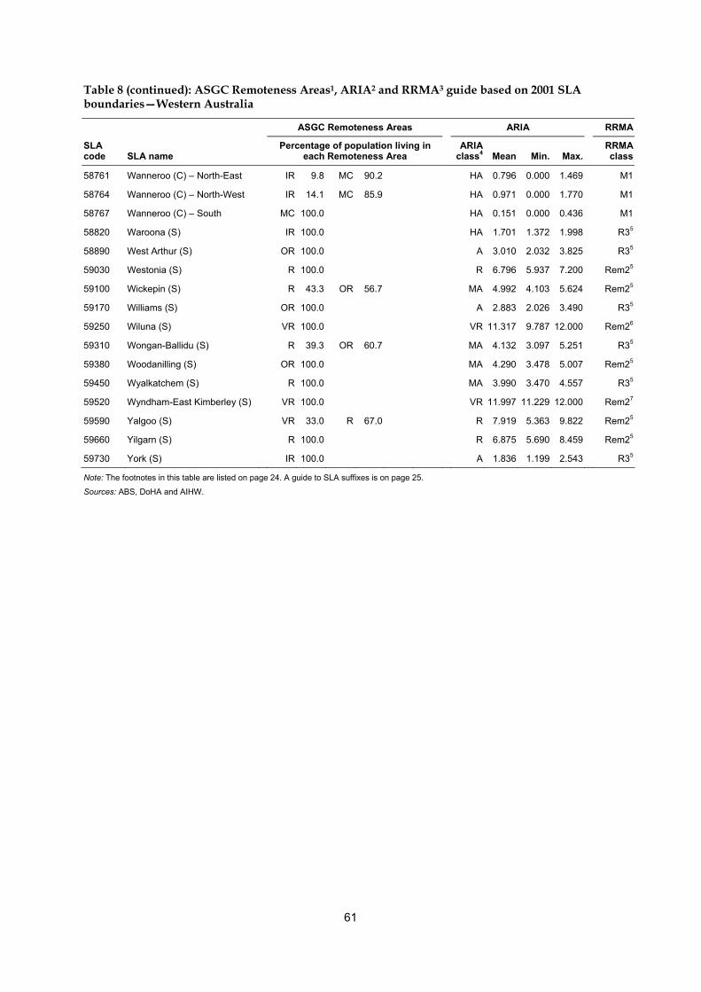
61
Table 8 (continued): ASGC Remoteness Areas1, ARIA2 and RRMA3 guide based on 2001 SLA boundaries—Western Australia
ASGC Remoteness Areas ARIA RRMA
SLA code SLA name
Percentage of population living in each Remoteness Area
ARIA class4
Mean
Min. Max.
RRMA class
58761 Wanneroo (C) – North-East IR 9.8 MC 90.2 HA 0.796 0.000 1.469 M1
58764 Wanneroo (C) – North-West IR 14.1 MC 85.9 HA 0.971 0.000 1.770 M1
58767 Wanneroo (C) – South MC 100.0 HA 0.151 0.000 0.436 M1
58820 Waroona (S) IR 100.0 HA 1.701 1.372 1.998 R35
58890 West Arthur (S) OR 100.0 A 3.010 2.032 3.825 R35
59030 Westonia (S) R 100.0 R 6.796 5.937 7.200 Rem25
59100 Wickepin (S) R 43.3 OR 56.7 MA 4.992 4.103 5.624 Rem25
59170 Williams (S) OR 100.0 A 2.883 2.026 3.490 R35
59250 Wiluna (S) VR 100.0 VR 11.317 9.787 12.000 Rem26
59310 Wongan-Ballidu (S) R 39.3 OR 60.7 MA 4.132 3.097 5.251 R35
59380 Woodanilling (S) OR 100.0 MA 4.290 3.478 5.007 Rem25
59450 Wyalkatchem (S) R 100.0 MA 3.990 3.470 4.557 R35
59520 Wyndham-East Kimberley (S) VR 100.0 VR 11.997 11.229 12.000 Rem27
59590 Yalgoo (S) VR 33.0 R 67.0 R 7.919 5.363 9.822 Rem25
59660 Yilgarn (S) R 100.0 R 6.875 5.690 8.459 Rem25
59730 York (S) IR 100.0 A 1.836 1.199 2.543 R35
Note: The footnotes in this table are listed on page 24. A guide to SLA suffixes is on page 25.
Sources: ABS, DoHA and AIHW.

62
Table 9: ASGC Remoteness Areas1, ARIA2 and RRMA3 guide based on 2001 SLA boundaries—Tasmania
ASGC Remoteness Areas ARIA RRMA
SLA code SLA name
Percentage of population living in each Remoteness Area
ARIA class4
Mean
Min. Max.
RRMA class
60210 Break O'Day (M) R 6.8 OR 93.2 MA 3.942 2.451 4.747 R36
60410 Brighton (M) IR 100.0 HA 1.663 1.417 1.856 M1
60611 Burnie (C) – Pt A OR 100.0 A 2.160 2.080 2.406 R25
60612 Burnie (C) – Pt B OR 100.0 A 2.643 2.175 3.236 R35
60811 Central Coast (M) – Pt A OR 100.0 A 2.127 2.000 2.259 R36
60812 Central Coast (M) – Pt B OR 100.0 A 2.502 2.044 2.944 R36
61010 Central Highlands (M) R 9.8 OR 90.2 A 3.490 2.069 4.919 R36
61210 Circular Head (M) OR 92.8 R 7.2 MA 4.674 2.999 5.706 R35
61410 Clarence (C) OR 5.2 IR 94.8 HA 1.616 1.210 2.062 M1
61511 Derwent Valley (M) – Pt A IR 100.0 HA 1.610 1.517 1.703 M1
61512 Derwent Valley (M) – Pt B OR 66.2 IR 33.1 R 0.7 A 3.361 1.581 4.780 R36
61610 Devonport (C) OR 6.3 IR 93.7 A 1.911 1.780 2.101 R26
61810 Dorset (M) R 4.0 OR 96.0 A 3.353 2.113 4.890 R36
62010 Flinders (M) VR 100.0 VR 9.803 9.200 10.010 Rem25
62211 George Town (M) – Pt A OR 100.0 A 1.999 1.866 2.137 R35
62212 George Town (M) – Pt B OR 100.0 A 2.148 1.866 2.460 R35
62410 Glamorgan/Spring Bay (M) OR 38.4 R 61.6 MA 3.780 2.203 5.178 R35
62610 Glenorchy (C) IR 100.0 HA 1.471 1.210 1.696 M1
62811 Hobart (C) – Inner IR 100.0 HA 1.210 1.210 1.210 M1
62812 Hobart (C) – Remainder IR 100.0 HA 1.290 1.210 1.581 M1
63010 Huon Valley (M) OR 97.2 R 2.8 A 3.027 1.627 4.244 R36
63210 Kentish (M) OR 100.0 A 2.615 1.874 3.527 R35
63410 King Island (M) VR 100.0 VR 9.460 9.460 9.460 Rem25
63611 Kingborough (M) – Pt A OR 3.9 IR 96.1 HA 1.580 1.210 2.532 M1
63612 Kingborough (M) – Pt B R 26.4 OR 73.6 A 3.600 1.810 4.010 R35
63811 Latrobe (M) – Pt A OR 100.0 A 1.932 1.780 2.074 R36
63812 Latrobe (M) – Pt B OR 100.0 A 2.091 1.855 2.408 R36
64011 Launceston (C) – Inner IR 100.0 HA 1.210 1.210 1.210 R15
64012 Launceston (C) – Pt B IR 100.0 HA 1.393 1.210 1.908 R16
64013 Launceston (C) – Pt C IR 17.4 OR 82.6 A 2.020 1.210 2.482 R36
64211 Meander Valley (M) – Pt A IR 100.0 HA 1.278 1.210 1.448 R17
64212 Meander Valley (M) – Pt B IR 6.5 OR 93.5 A 2.737 1.261 4.321 R36
64611 Northern Midlands (M) – Pt A IR 100.0 HA 1.499 1.221 1.700 R36
64612 Northern Midlands (M) – Pt B OR 100.0 A 2.815 1.544 4.491 R36
(continued) Note: The footnotes in this table are listed on page 24. A guide to SLA suffixes is on page 25.
Sources: ABS, DoHA and AIHW.
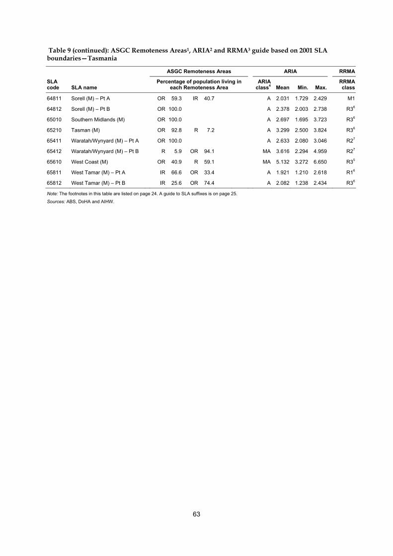
63
Table 9 (continued): ASGC Remoteness Areas1, ARIA2 and RRMA3 guide based on 2001 SLA boundaries—Tasmania
ASGC Remoteness Areas ARIA RRMA
SLA code SLA name
Percentage of population living in each Remoteness Area
ARIA class4
Mean
Min. Max.
RRMA class
64811 Sorell (M) – Pt A OR 59.3 IR 40.7 A 2.031 1.729 2.429 M1
64812 Sorell (M) – Pt B OR 100.0 A 2.378 2.003 2.738 R36
65010 Southern Midlands (M) OR 100.0 A 2.697 1.695 3.723 R36
65210 Tasman (M) OR 92.8 R 7.2 A 3.299 2.500 3.824 R36
65411 Waratah/Wynyard (M) – Pt A OR 100.0 A 2.633 2.080 3.046 R27
65412 Waratah/Wynyard (M) – Pt B R 5.9 OR 94.1 MA 3.616 2.294 4.959 R27
65610 West Coast (M) OR 40.9 R 59.1 MA 5.132 3.272 6.650 R35
65811 West Tamar (M) – Pt A IR 66.6 OR 33.4 A 1.921 1.210 2.618 R16
65812 West Tamar (M) – Pt B IR 25.6 OR 74.4 A 2.082 1.238 2.434 R36
Note: The footnotes in this table are listed on page 24. A guide to SLA suffixes is on page 25.
Sources: ABS, DoHA and AIHW.
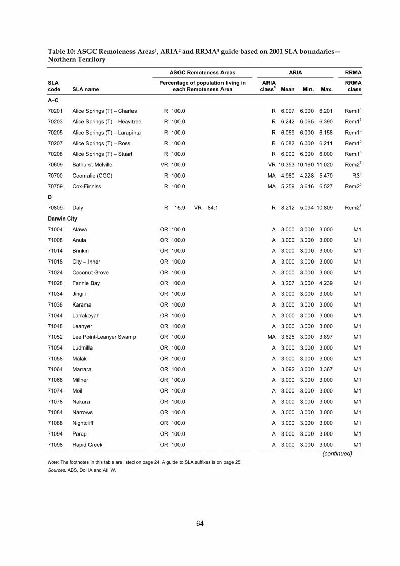
64
Table 10: ASGC Remoteness Areas1, ARIA2 and RRMA3 guide based on 2001 SLA boundaries—Northern Territory
ASGC Remoteness Areas ARIA RRMA
SLA code SLA name
Percentage of population living in each Remoteness Area
ARIA class4
Mean
Min. Max.
RRMA class
A–C
70201 Alice Springs (T) – Charles R 100.0 R 6.097 6.000 6.201 Rem16
70203 Alice Springs (T) – Heavitree R 100.0 R 6.242 6.065 6.390 Rem16
70205 Alice Springs (T) – Larapinta R 100.0 R 6.069 6.000 6.158 Rem16
70207 Alice Springs (T) – Ross R 100.0 R 6.082 6.000 6.211 Rem16
70208 Alice Springs (T) – Stuart R 100.0 R 6.000 6.000 6.000 Rem16
70609 Bathurst-Melville VR 100.0 VR 10.353 10.160 11.020 Rem25
70700 Coomalie (CGC) R 100.0 MA 4.960 4.228 5.470 R35
70759 Cox-Finniss R 100.0 MA 5.259 3.646 6.527 Rem25
D
70809 Daly R 15.9 VR 84.1 R 8.212 5.094 10.809 Rem25
Darwin City
71004 Alawa OR 100.0 A 3.000 3.000 3.000 M1
71008 Anula OR 100.0 A 3.000 3.000 3.000 M1
71014 Brinkin OR 100.0 A 3.000 3.000 3.000 M1
71018 City – Inner OR 100.0 A 3.000 3.000 3.000 M1
71024 Coconut Grove OR 100.0 A 3.000 3.000 3.000 M1
71028 Fannie Bay OR 100.0 A 3.207 3.000 4.239 M1
71034 Jingili OR 100.0 A 3.000 3.000 3.000 M1
71038 Karama OR 100.0 A 3.000 3.000 3.000 M1
71044 Larrakeyah OR 100.0 A 3.000 3.000 3.000 M1
71048 Leanyer OR 100.0 A 3.000 3.000 3.000 M1
71052 Lee Point-Leanyer Swamp OR 100.0 MA 3.625 3.000 3.897 M1
71054 Ludmilla OR 100.0 A 3.000 3.000 3.000 M1
71058 Malak OR 100.0 A 3.000 3.000 3.000 M1
71064 Marrara OR 100.0 A 3.092 3.000 3.367 M1
71068 Millner OR 100.0 A 3.000 3.000 3.000 M1
71074 Moil OR 100.0 A 3.000 3.000 3.000 M1
71078 Nakara OR 100.0 A 3.000 3.000 3.000 M1
71084 Narrows OR 100.0 A 3.000 3.000 3.000 M1
71088 Nightcliff OR 100.0 A 3.000 3.000 3.000 M1
71094 Parap OR 100.0 A 3.000 3.000 3.000 M1
71098 Rapid Creek OR 100.0 A 3.000 3.000 3.000 M1
(continued) Note: The footnotes in this table are listed on page 24. A guide to SLA suffixes is on page 25.
Sources: ABS, DoHA and AIHW.
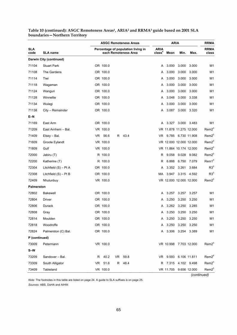
65
Table 10 (continued): ASGC Remoteness Areas1, ARIA2 and RRMA3 guide based on 2001 SLA boundaries—Northern Territory
ASGC Remoteness Areas ARIA RRMA
SLA code SLA name
Percentage of population living in each Remoteness Area
ARIA class4
Mean
Min. Max.
RRMA class
Darwin City (continued)
71104 Stuart Park OR 100.0 A 3.000 3.000 3.000 M1
71108 The Gardens OR 100.0 A 3.000 3.000 3.000 M1
71114 Tiwi OR 100.0 A 3.000 3.000 3.000 M1
71118 Wagaman OR 100.0 A 3.000 3.000 3.000 M1
71124 Wanguri OR 100.0 A 3.000 3.000 3.000 M1
71128 Winnellie OR 100.0 A 3.048 3.000 3.338 M1
71134 Wulagi OR 100.0 A 3.000 3.000 3.000 M1
71138 City – Remainder OR 100.0 A 3.087 3.000 3.320 M1
E–N
71169 East Arm OR 100.0 A 3.327 3.000 3.483 M1
71209 East Arnhem – Bal. VR 100.0 VR 11.878 11.275 12.000 Rem25
71409 Elsey – Bal. VR 56.6 R 43.4 VR 9.785 6.730 11.908 Rem25
71609 Groote Eylandt VR 100.0 VR 12.000 12.000 12.000 Rem25
71809 Gulf VR 100.0 VR 11.864 10.174 12.000 Rem25
72000 Jabiru (T) R 100.0 R 9.058 9.028 9.082 Rem25
72200 Katherine (T) R 100.0 R 6.888 6.750 7.079 Rem15
72304 Litchfield (S) – Pt A OR 100.0 A 3.352 3.261 3.684 R35
72308 Litchfield (S) – Pt B OR 100.0 MA 3.947 3.315 4.592 R35
72409 Nhulunbuy VR 100.0 VR 12.000 12.000 12.000 Rem25
Palmerston
72802 Bakewell OR 100.0 A 3.257 3.257 3.257 M1
72804 Driver OR 100.0 A 3.250 3.250 3.250 M1
72806 Durack OR 100.0 A 3.262 3.250 3.285 M1
72808 Gray OR 100.0 A 3.250 3.250 3.250 M1
72814 Moulden OR 100.0 A 3.250 3.250 3.250 M1
72818 Woodroffe OR 100.0 A 3.250 3.250 3.250 M1
72824 Palmerston (C) Bal. OR 100.0 A 3.306 3.254 3.389 M1
P (continued)
73009 Petermann VR 100.0 VR 10.998 7.703 12.000 Rem25
S–W
73209 Sandover – Bal. R 40.2 VR 59.8 VR 9.593 6.106 11.811 Rem26
73309 South Alligator VR 51.6 R 48.4 R 7.315 4.102 9.498 Rem25
73409 Tableland VR 100.0 VR 11.705 9.656 12.000 Rem25
(continued) Note: The footnotes in this table are listed on page 24. A guide to SLA suffixes is on page 25.
Sources: ABS, DoHA and AIHW.

66
Table 10 (continued): ASGC Remoteness Areas1, ARIA2 and RRMA3 guide based on 2001 SLA boundaries—Northern Territory
ASGC Remoteness Areas ARIA RRMA
SLA code SLA name
Percentage of population living in each Remoteness Area
ARIA class4
Mean
Min. Max.
RRMA class
S–W (continued)
73609 Tanami VR 100.0 VR 11.298 7.318 12.000 Rem25
73800 Tennant Creek (T) VR 100.0 VR 12.000 12.000 12.000 Rem25
74009 Tennant Creek – Bal. VR 100.0 VR 11.537 9.344 12.000 Rem25
74409 Victoria VR 100.0 VR 11.512 7.316 12.000 Rem25
74809 West Arnhem VR 100.0 VR 10.395 5.808 11.771 Rem25
Note: The footnotes in this table are listed on page 24. A guide to SLA suffixes is on page 25.
Sources: ABS, DoHA and AIHW.
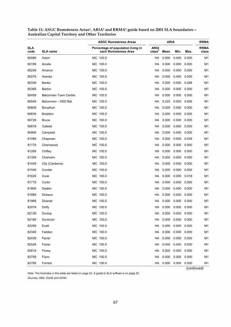
67
Table 11: ASGC Remoteness Areas1, ARIA2 and RRMA3 guide based on 2001 SLA boundaries—Australian Capital Territory and Other Territories
ASGC Remoteness Areas ARIA RRMA
SLA code SLA name
Percentage of population living in each Remoteness Area
ARIA class4
Mean
Min. Max.
RRMA class
80089 Acton MC 100.0 HA 0.000 0.000 0.000 M1
80189 Ainslie MC 100.0 HA 0.000 0.000 0.000 M1
80239 Amaroo MC 100.0 HA 0.000 0.000 0.000 M1
80279 Aranda MC 100.0 HA 0.000 0.000 0.000 M1
80339 Banks MC 100.0 HA 0.000 0.000 0.268 M1
80369 Barton MC 100.0 HA 0.000 0.000 0.000 M1
80459 Belconnen Town Centre MC 100.0 HA 0.000 0.000 0.000 M1
80549 Belconnen – SSD Bal. MC 100.0 HA 0.225 0.000 0.606 M1
80609 Bonython MC 100.0 HA 0.000 0.000 0.000 M1
80639 Braddon MC 100.0 HA 0.000 0.000 0.000 M1
80729 Bruce MC 100.0 HA 0.000 0.000 0.000 M1
80819 Calwell MC 100.0 HA 0.000 0.000 0.000 M1
80909 Campbell MC 100.0 HA 0.000 0.000 0.000 M1
81089 Chapman MC 100.0 HA 0.000 0.000 0.038 M1
81179 Charnwood MC 100.0 HA 0.000 0.000 0.000 M1
81269 Chifley MC 100.0 HA 0.000 0.000 0.000 M1
81359 Chisholm MC 100.0 HA 0.000 0.000 0.000 M1
81449 City (Canberra) MC 100.0 HA 0.000 0.000 0.000 M1
81549 Conder MC 100.0 HA 0.000 0.000 0.000 M1
81629 Cook MC 100.0 HA 0.000 0.000 0.018 M1
81719 Curtin MC 100.0 HA 0.000 0.000 0.000 M1
81809 Deakin MC 100.0 HA 0.000 0.000 0.000 M1
81889 Dickson MC 100.0 HA 0.000 0.000 0.000 M1
81989 Downer MC 100.0 HA 0.000 0.000 0.000 M1
82079 Duffy MC 100.0 HA 0.000 0.000 0.000 M1
82139 Dunlop MC 100.0 HA 0.000 0.000 0.000 M1
82169 Duntroon MC 100.0 HA 0.000 0.000 0.000 M1
82259 Evatt MC 100.0 HA 0.000 0.000 0.000 M1
82349 Fadden MC 100.0 HA 0.000 0.000 0.000 M1
82439 Farrer MC 100.0 HA 0.000 0.000 0.000 M1
82529 Fisher MC 100.0 HA 0.000 0.000 0.000 M1
82619 Florey MC 100.0 HA 0.000 0.000 0.000 M1
82709 Flynn MC 100.0 HA 0.000 0.000 0.000 M1
82789 Forrest MC 100.0 HA 0.000 0.000 0.000 M1
(continued) Note: The footnotes in this table are listed on page 24. A guide to SLA suffixes is on page 25.
Sources: ABS, DoHA and AIHW.
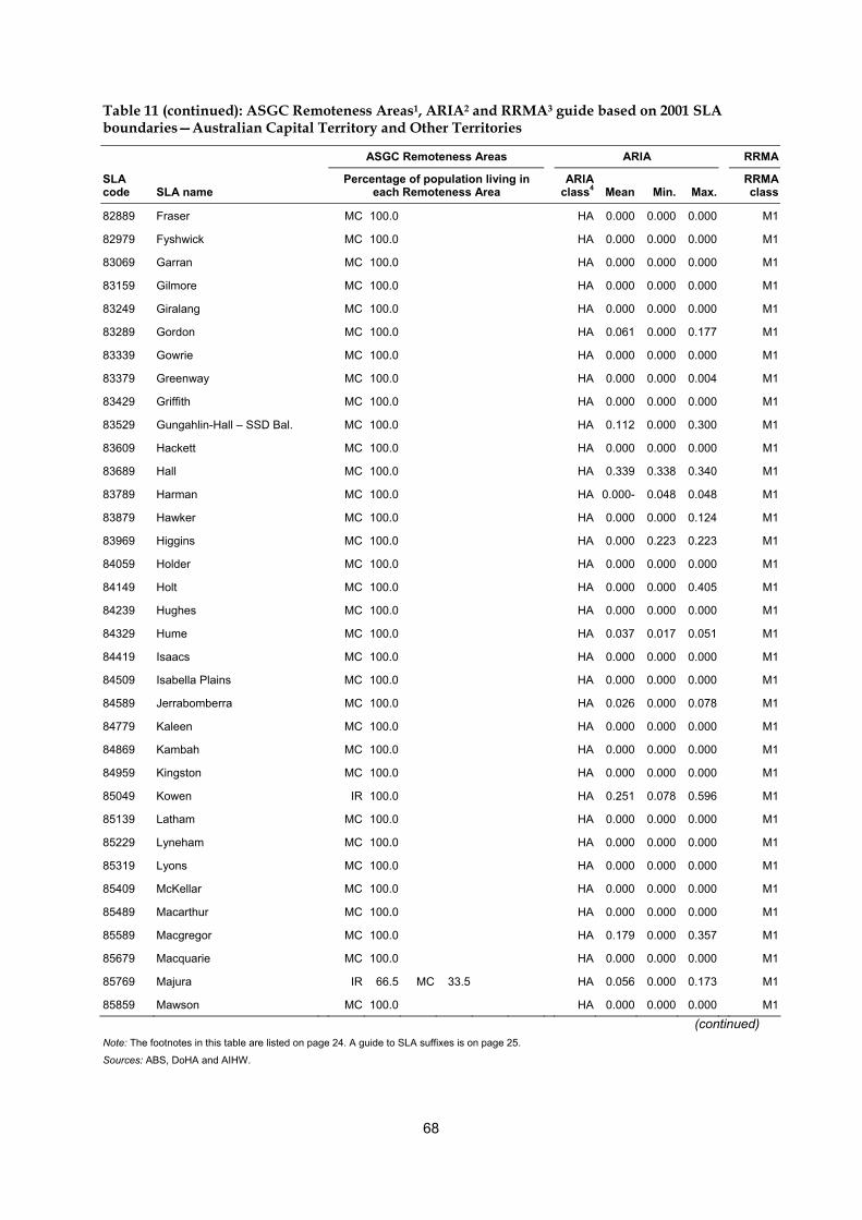
68
Table 11 (continued): ASGC Remoteness Areas1, ARIA2 and RRMA3 guide based on 2001 SLA boundaries—Australian Capital Territory and Other Territories
ASGC Remoteness Areas ARIA RRMA
SLA code SLA name
Percentage of population living in each Remoteness Area
ARIA class4
Mean
Min. Max.
RRMA class
82889 Fraser MC 100.0 HA 0.000 0.000 0.000 M1
82979 Fyshwick MC 100.0 HA 0.000 0.000 0.000 M1
83069 Garran MC 100.0 HA 0.000 0.000 0.000 M1
83159 Gilmore MC 100.0 HA 0.000 0.000 0.000 M1
83249 Giralang MC 100.0 HA 0.000 0.000 0.000 M1
83289 Gordon MC 100.0 HA 0.061 0.000 0.177 M1
83339 Gowrie MC 100.0 HA 0.000 0.000 0.000 M1
83379 Greenway MC 100.0 HA 0.000 0.000 0.004 M1
83429 Griffith MC 100.0 HA 0.000 0.000 0.000 M1
83529 Gungahlin-Hall – SSD Bal. MC 100.0 HA 0.112 0.000 0.300 M1
83609 Hackett MC 100.0 HA 0.000 0.000 0.000 M1
83689 Hall MC 100.0 HA 0.339 0.338 0.340 M1
83789 Harman MC 100.0 HA 0.000- 0.048 0.048 M1
83879 Hawker MC 100.0 HA 0.000 0.000 0.124 M1
83969 Higgins MC 100.0 HA 0.000 0.223 0.223 M1
84059 Holder MC 100.0 HA 0.000 0.000 0.000 M1
84149 Holt MC 100.0 HA 0.000 0.000 0.405 M1
84239 Hughes MC 100.0 HA 0.000 0.000 0.000 M1
84329 Hume MC 100.0 HA 0.037 0.017 0.051 M1
84419 Isaacs MC 100.0 HA 0.000 0.000 0.000 M1
84509 Isabella Plains MC 100.0 HA 0.000 0.000 0.000 M1
84589 Jerrabomberra MC 100.0 HA 0.026 0.000 0.078 M1
84779 Kaleen MC 100.0 HA 0.000 0.000 0.000 M1
84869 Kambah MC 100.0 HA 0.000 0.000 0.000 M1
84959 Kingston MC 100.0 HA 0.000 0.000 0.000 M1
85049 Kowen IR 100.0 HA 0.251 0.078 0.596 M1
85139 Latham MC 100.0 HA 0.000 0.000 0.000 M1
85229 Lyneham MC 100.0 HA 0.000 0.000 0.000 M1
85319 Lyons MC 100.0 HA 0.000 0.000 0.000 M1
85409 McKellar MC 100.0 HA 0.000 0.000 0.000 M1
85489 Macarthur MC 100.0 HA 0.000 0.000 0.000 M1
85589 Macgregor MC 100.0 HA 0.179 0.000 0.357 M1
85679 Macquarie MC 100.0 HA 0.000 0.000 0.000 M1
85769 Majura IR 66.5 MC 33.5 HA 0.056 0.000 0.173 M1
85859 Mawson MC 100.0 HA 0.000 0.000 0.000 M1
(continued) Note: The footnotes in this table are listed on page 24. A guide to SLA suffixes is on page 25.
Sources: ABS, DoHA and AIHW.
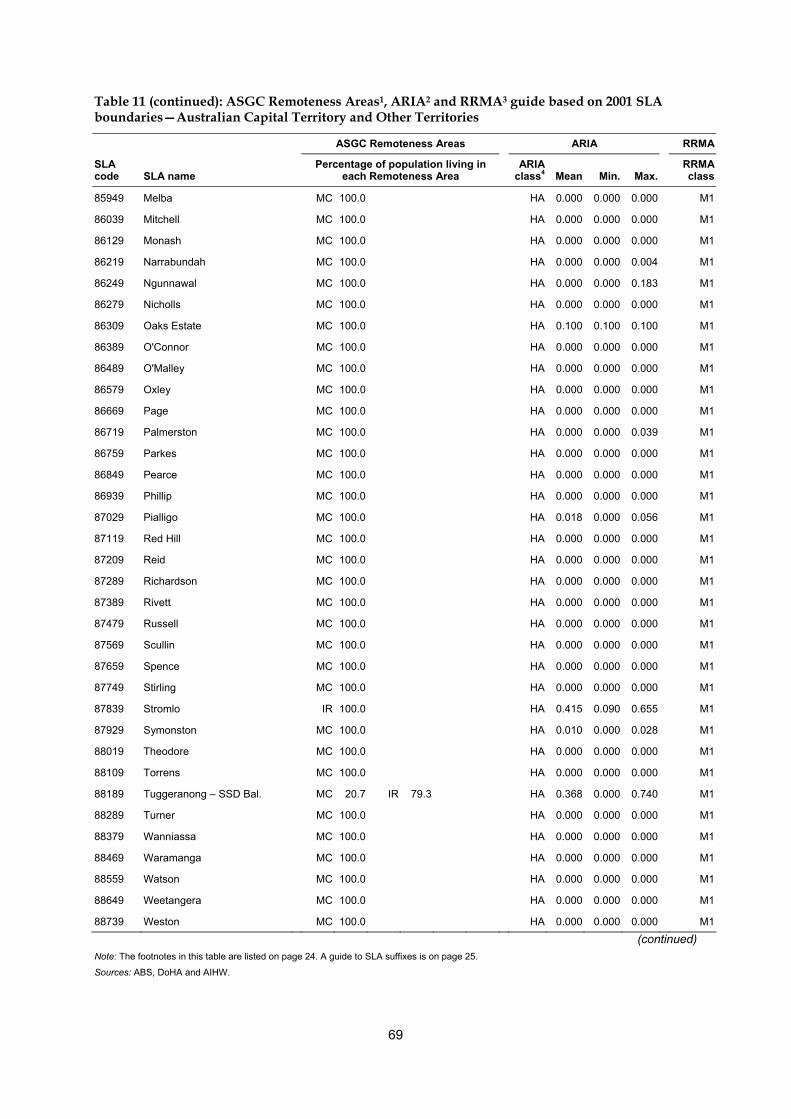
69
Table 11 (continued): ASGC Remoteness Areas1, ARIA2 and RRMA3 guide based on 2001 SLA boundaries—Australian Capital Territory and Other Territories
ASGC Remoteness Areas ARIA RRMA
SLA code SLA name
Percentage of population living in each Remoteness Area
ARIA class4
Mean
Min. Max.
RRMA class
85949 Melba MC 100.0 HA 0.000 0.000 0.000 M1
86039 Mitchell MC 100.0 HA 0.000 0.000 0.000 M1
86129 Monash MC 100.0 HA 0.000 0.000 0.000 M1
86219 Narrabundah MC 100.0 HA 0.000 0.000 0.004 M1
86249 Ngunnawal MC 100.0 HA 0.000 0.000 0.183 M1
86279 Nicholls MC 100.0 HA 0.000 0.000 0.000 M1
86309 Oaks Estate MC 100.0 HA 0.100 0.100 0.100 M1
86389 O'Connor MC 100.0 HA 0.000 0.000 0.000 M1
86489 O'Malley MC 100.0 HA 0.000 0.000 0.000 M1
86579 Oxley MC 100.0 HA 0.000 0.000 0.000 M1
86669 Page MC 100.0 HA 0.000 0.000 0.000 M1
86719 Palmerston MC 100.0 HA 0.000 0.000 0.039 M1
86759 Parkes MC 100.0 HA 0.000 0.000 0.000 M1
86849 Pearce MC 100.0 HA 0.000 0.000 0.000 M1
86939 Phillip MC 100.0 HA 0.000 0.000 0.000 M1
87029 Pialligo MC 100.0 HA 0.018 0.000 0.056 M1
87119 Red Hill MC 100.0 HA 0.000 0.000 0.000 M1
87209 Reid MC 100.0 HA 0.000 0.000 0.000 M1
87289 Richardson MC 100.0 HA 0.000 0.000 0.000 M1
87389 Rivett MC 100.0 HA 0.000 0.000 0.000 M1
87479 Russell MC 100.0 HA 0.000 0.000 0.000 M1
87569 Scullin MC 100.0 HA 0.000 0.000 0.000 M1
87659 Spence MC 100.0 HA 0.000 0.000 0.000 M1
87749 Stirling MC 100.0 HA 0.000 0.000 0.000 M1
87839 Stromlo IR 100.0 HA 0.415 0.090 0.655 M1
87929 Symonston MC 100.0 HA 0.010 0.000 0.028 M1
88019 Theodore MC 100.0 HA 0.000 0.000 0.000 M1
88109 Torrens MC 100.0 HA 0.000 0.000 0.000 M1
88189 Tuggeranong – SSD Bal. MC 20.7 IR 79.3 HA 0.368 0.000 0.740 M1
88289 Turner MC 100.0 HA 0.000 0.000 0.000 M1
88379 Wanniassa MC 100.0 HA 0.000 0.000 0.000 M1
88469 Waramanga MC 100.0 HA 0.000 0.000 0.000 M1
88559 Watson MC 100.0 HA 0.000 0.000 0.000 M1
88649 Weetangera MC 100.0 HA 0.000 0.000 0.000 M1
88739 Weston MC 100.0 HA 0.000 0.000 0.000 M1
(continued) Note: The footnotes in this table are listed on page 24. A guide to SLA suffixes is on page 25.
Sources: ABS, DoHA and AIHW.
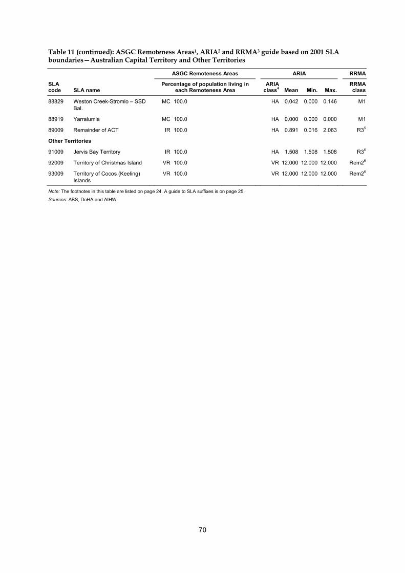
70
Table 11 (continued): ASGC Remoteness Areas1, ARIA2 and RRMA3 guide based on 2001 SLA boundaries—Australian Capital Territory and Other Territories
ASGC Remoteness Areas ARIA RRMA
SLA code SLA name
Percentage of population living in each Remoteness Area
ARIA class4
Mean
Min. Max.
RRMA class
88829 Weston Creek-Stromlo – SSD Bal.
MC 100.0 HA 0.042 0.000 0.146 M1
88919 Yarralumla MC 100.0 HA 0.000 0.000 0.000 M1
89009 Remainder of ACT IR 100.0 HA 0.891 0.016 2.063 R35
Other Territories
91009 Jervis Bay Territory IR 100.0 HA 1.508 1.508 1.508 R36
92009 Territory of Christmas Island VR 100.0 VR 12.000 12.000 12.000 Rem26
93009 Territory of Cocos (Keeling) Islands
VR 100.0 VR 12.000 12.000 12.000 Rem26
Note: The footnotes in this table are listed on page 24. A guide to SLA suffixes is on page 25.
Sources: ABS, DoHA and AIHW.

71
Appendix A—Case studies of SLAs Each SLA possesses characteristics and circumstances that determine its RRMA and ARIA class and how its population is apportioned to ASGC Remoteness Areas classes. The following discussion of a selection of SLAs (Table 12) illustrates the diversity of characteristics and circumstances that can occur.
Table 12: ASGC Remoteness Areas1, ARIA2 and RRMA3 guide—selected SLAs
ASGC Remoteness Areas ARIA RRMA
SLA code SLA name
Percentage of population living in each Remoteness Area
ARIA class4
Mean
Min. Max.
RRMA class
10300 Balranald (A) R 16.1 OR 83.9 MA 5.722 3.416 8.222 Rem25
10500 Baulkham Hills (A) MC 92.4 IR 7.6 HA 1.092 0.000 2.033 M1
11250 Broken Hill (C) OR 100.0 A 3.343 3.240 3.511 R25
13751 Hastings (A) – Pt A IR 100.0 A 1.737 1.640 1.876 R16
13754 Hastings (A) – Pt B OR 14.2 IR 85.8 A 2.436 1.670 3.374 R17
33801 Hinchinbrook (S) (excl. Palm I.) R 0.7 OR 99.3 MA 4.685 4.282 5.445 R36
33804 Hinchinbrook (S) – Palm Island R 100.0 VR 9.200 9.200 9.200 R36
48540 Whyalla (C) OR 100.0 A 2.929 2.450 3.536 R17
54281 Kalgoorlie/Boulder (C) – Pt A OR 100.0 MA 3.937 3.870 4.022 Rem16
54284 Kalgoorlie/Boulder (C) – Pt B VR 55.1 OR 0.0 R 44.9 VR 9.832 3.924 12.000 Rem17
Note: The footnotes in this table are listed on page 24. A guide to SLA suffixes is on page 25.
Sources: ABS, DoHA and AIHW.
Balranald The New South Wales Area of Balranald’s boundary has not changed since 1991. This SLA has inherited the RRMA class allocated to this SLA in 1994 (and based on 1991 census information). This SLA is RRMA class Rem2 (Other Remote Area with an urban centre population of less than 5,000 people). In 2001 the urban centre of this SLA still contained fewer than 5,000 people. This SLA is highly heterogeneous because the ARIA index values of points contained within this SLA range from 3.416 (indicating an Accessible area) to 8.222 (indicating a Remote area). The SLA is ARIA class MA (Moderately Accessible) because it has a mean index value of 5.722. Because the SLA is heterogeneous the mean index value may not be indicative of levels of accessibility experienced by the population of this SLA. In 2001 83.9% of this SLA’s population lived in Outer Regional Australia CDs (that is, in CDs with a mean index value of greater than 2.4 and less than or equal to 5.92) and 16.1% lived in Remote Australia CDs (that is, in CDs with a mean index value of greater than 5.92 and less than or equal to 10.53).
72
Baulkham Hills The New South Wales Area of Baulkham Hills is RRMA class M1 (Capital Cities) because it is contained within the boundaries of a Capital City Statistical Division11 (Sydney). The SLA is ARIA class HA (Highly Accessible) because it has a mean index value of 1.092. The SLA is slightly heterogeneous because the ARIA index values of grid points contained within this SLA range from 0.000 (indicating a Highly Accessible area) to 2.033 (indicating an Accessible area). In 2001 92.4% of this SLA’s population lived in Major Cities of Australia and 7.6% lived in Inner Regional Australia.
Broken Hill The New South Wales City of Broken Hill’s boundary has not changed since 1991. This SLA has inherited the RRMA class allocated to this SLA in 1994 (and based on 1991 census information). This SLA is RRMA class R2 (Small Rural Centre with an urban centre population of 10,000–24,999). In 2001 the urban centre of this SLA still had a population of 10,000–24,999). The SLA is ARIA class A (Accessible) because it has a mean index value of 3.343. The SLA is on the borderline of Accessible/Moderately Accessible because the cut-off ARIA index value is 3.51 and the SLA is mostly homogeneous (with the ARIA index values of grid points contained within this SLA ranging from 3.240 to 3.511). In 2001 100% of this SLA’s population lived in Outer Regional Australia.
Hastings The boundaries of the New South Wales Area of Hastings SLA have changed since 1991. In 2001 this SLA was split, with 42% of the area (including the urban centre of Port Macquarie) going to Hastings—Part A and the remainder to Hastings—Part B. Both of these inherited the RRMA class of R1 (Large Rural Centre with an urban centre population of 25,000–99,999) which was originally allocated to the 1991 SLA of Hastings (and based on 1991 census information). In 2001 the New South Wales Area of Hastings—Part A still contained an urban centre with a population of 25,000—99,999. However Hastings—Part B does not contain an urban centre of this size. The RRMA class assigned to Hastings—Part B does not reflect the true status of this SLA. Hastings—Part A is ARIA class A (Accessible) because it has a mean index value of 1.737. Hastings—Part B is ARIA class A (Accessible) because it has a mean index value of 2.436. The ARIA index values of points within Hastings—Part A range from 1.640 to 1.876. The ARIA index values of points within Hastings—Part B range from 1.670 to 3.374. The people in Hastings—Part A live closer to the service centre of Port Macquarie than the people in Hastings—Part B. This explains why the ARIA index values in Hastings—Part A tend to be lower than those in Hastings—Part B. In 2001 100% of the population of Hastings—Part A lived in Inner Regional Australia. In that same year 85.8% of the population of Hastings—Part B lived in Inner Regional Australia and 14.2% lived in Outer Regional Australia.
11 A Capital City Statistical Division represents the city in a wider sense. It should contain the anticipated development of the city for a period of at least 20 years (ABS 2003).
73
Hinchinbrook The boundaries of the Queensland SLA of Hinchinbrook Shire have changed since 1991. In 1998 this SLA was split into Hinchinbrook Shire (excluding Palm Island) and Hinchinbrook Shire—Palm Island. Both SLAs inherited the RRMA class originally allocated to the 1991 SLA of Hinchinbrook Shire (and which was based on 1991 census information). These SLAs are RRMA class R3 (Other Rural Areas with an urban centre population of less than 10,000 people). Because it is an island, Hinchinbrook Shire—Palm Island is significantly more remote than Hinchinbrook Shire (excluding Palm Island). Hinchinbrook Shire (excluding Palm Island) is ARIA class MA (Moderately Accessible) because it has a mean index value of 4.685. Hinchinbrook Shire—Palm Island is ARIA class VR (Very Remote) because it has a mean index value of 9.200. In 2001 under ASGC Remoteness Areas, 0.7% of the population of Hinchinbrook Shire (excluding Palm Island) lived in Remote Australia and 99.3% in Outer Regional Australia. In that same year 100% of the population of Hinchinbrook Shire—Palm Island lived in Remote Australia.
Whyalla The South Australian City of Whyalla’s boundary has not changed since 1991. This SLA inherited the RRMA class allocated to it in 1994 (and based on 1991 census information). This SLA is RRMA class R1 (Large Rural Centre with an urban centre population of 25,000–99,999). In 2001 the population of the urban centre of Whyalla had declined to fewer than 25,000. The RRMA class assigned to this SLA therefore does not reflect the true status of this SLA. Therefore the RRMA class has become incorrect. The SLA is ARIA class A (Accessible) because it has a mean index value of 2.929. In 2001, 100% of this SLA’s population lived in Outer Regional Australia.
Kalgoorlie/Boulder The boundaries of the Western Australian SLAs of Kalgoorlie/Boulder City—Part A and Kalgoorlie/Boulder City—Part B have changed since 1991. In 1991 this SLA was called Kalgoorlie/Boulder City and its boundary encompassed the city of Kalgoorlie/Boulder and stretched to the Western Australia/South Australia border. In 2001 the SLA was split into Kalgoorlie/Boulder City—Part A (which included the urban centre of Kalgoorlie/Boulder) and Kalgoorlie/Boulder City—Part B (which included the remaining land in the original SLA boundary). Both SLAs inherited the RRMA class of Rem1 (Large Remote Centre with an urban centre population of more than 5,000) that was originally allocated to Kalgoorlie/Boulder City in 1994 (and based on 1991 census information). In 2001 Kalgoorlie/Boulder City—Part A still contained an urban centre with a population of more than 5,000 (Kalgoorlie/Boulder). However, because of the boundary change, Kalgoorlie/Boulder City—Part B does not contain an urban centre of this size. The RRMA class assigned to this SLA therefore does not reflect the true status of this SLA. The RRMA class of Kalgoorlie/Boulder City—Part A also does not reflect this SLA’s true status. Kalgoorlie/Boulder City SLA may have originally been classed as being in a remote zone in 1994 due to the SLAs low population density. The new SLA of Kalgoorlie/Boulder—Part A has a higher population density than the much larger 1991 SLA of Kalgoorlie/Boulder City. If RRMA information were to be recalculated using 2001 SLA boundaries and 2001 census data it could result in Kalgoorlie/Boulder—Part A being reclassed from Rem1 to R1 (Large Rural Centre with an urban centre population of 25,000–99,999). Kalgoorlie/Boulder City—
74
Part A is ARIA class MA (Moderately Accessible) because it has a mean index value of 3.937. Kalgoorlie/Boulder City—Part B is ARIA class VR (Very Remote) because it has a mean index value of 9.832. This SLA is highly heterogeneous because the ARIA index values of points contained within this SLA range from 3.870 (indicating a Moderately Accessible area) to 12.000 (indicating a Very Remote area). In 2001, 100% of the population of Kalgoorlie/Boulder City—Part A lived in Outer Regional Australia. In that same year 55.1% of the population of Kalgoorlie/Boulder City—Part B lived in Very Remote Australia, 44.9% in Remote Australia and a very small number in Outer Regional Australia.
75
Appendix B—Interpolating ARIA and ARIA+ to a 1 km grid The ARIA and ARIA+ methodology results in ARIA and ARIA+ index values for 11,340 populated localities. This does not cover all of Australia’s inhabitants because some live outside these localities. This problem is ‘overcome by using a “grid-cell” approach: the values of remoteness were interpolated onto a 1 km notional grid across the whole of Australia. The interpolation procedure was an Inverse Distance Weighted algorithm which used the remoteness values of the six nearest localities12, weighted by the distance of each point to the cell being analysed, to assign a remoteness value to that cell. (Where a cell was within a service centre in the relevant category, it was however assigned a distance value of zero.)’ (DHAC & GISCA 2001).
12 Except in the cases of islands, where a value based on the island localities only was used.
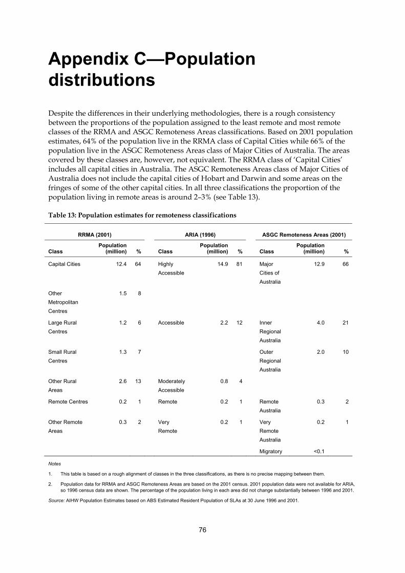
76
Appendix C—Population distributions Despite the differences in their underlying methodologies, there is a rough consistency between the proportions of the population assigned to the least remote and most remote classes of the RRMA and ASGC Remoteness Areas classifications. Based on 2001 population estimates, 64% of the population live in the RRMA class of Capital Cities while 66% of the population live in the ASGC Remoteness Areas class of Major Cities of Australia. The areas covered by these classes are, however, not equivalent. The RRMA class of ‘Capital Cities’ includes all capital cities in Australia. The ASGC Remoteness Areas class of Major Cities of Australia does not include the capital cities of Hobart and Darwin and some areas on the fringes of some of the other capital cities. In all three classifications the proportion of the population living in remote areas is around 2–3% (see Table 13).
Table 13: Population estimates for remoteness classifications
RRMA (2001)
ARIA (1996)
ASGC Remoteness Areas (2001)
Class
Population (million)
%
Class
Population (million) %
Class
Population (million) %
Capital Cities 12.4 64 Highly Accessible
14.9 81 Major Cities of Australia
12.9 66
Other Metropolitan Centres
1.5 8
Large Rural Centres
1.2 6 Accessible 2.2 12 Inner Regional Australia
4.0 21
Small Rural Centres
1.3 7 Outer Regional Australia
2.0 10
Other Rural Areas
2.6 13 Moderately Accessible
0.8 4
Remote Centres 0.2 1 Remote 0.2 1 Remote Australia
0.3 2
Other Remote Areas
0.3 2 Very Remote
0.2 1 Very Remote Australia
0.2 1
Migratory <0.1
Notes
1. This table is based on a rough alignment of classes in the three classifications, as there is no precise mapping between them.
2. Population data for RRMA and ASGC Remoteness Areas are based on the 2001 census. 2001 population data were not available for ARIA, so 1996 census data are shown. The percentage of the population living in each area did not change substantially between 1996 and 2001.
Source: AIHW Population Estimates based on ABS Estimated Resident Population of SLAs at 30 June 1996 and 2001.
77
References ABS (Australian Bureau of Statistics) 2001a. ABS views on remoteness, 2001a. Information paper. ABS cat. no. 1244.0. Canberra: ABS. ABS (Australian Bureau of Statistics) 2001b. Outcomes of ABS views on remoteness consultation, Australia. Information paper. ABS cat. no. 1244.0.00.001. Canberra: ABS. ABS (Australian Bureau of Statistics) 2002. Australian Standard Geographical Classification (ASGC) 2002. ABS cat. no. 1216.0. Canberra: ABS. ABS (Australian Bureau of Statistics) 2003. ASGC Remoteness classification: purpose and use. Census Paper 03/01. Canberra: ABS. AIHW (Australian Institute of Health and Welfare) 2003. Rural, regional and remote health: a study on mortality. AIHW cat. no. PHE 45. Canberra: AIHW. DHAC (Department of Health and Aged Care) 2001. Department of Health and Aged Care website: www.health.gov.au/ari/aria.htm. DHAC (Department of Health and Aged Care) & GISCA (National Key Centre for Social Applications of Geographic Information Systems) 2001. Measuring remoteness: Accessibility/Remoteness Index of Australia (ARIA). Occasional Papers: New Series No. 14. Canberra: DHAC. DPIE (Department of Primary Industries and Energy) & DHSH (Department of Human Services and Health) 1994. Rural, Remote and Metropolitan Areas classification. 1991 Census edition. Canberra: Australian Government Publishing Service.