Runs versus Lemons:

Information Disclosure and Fiscal Capacity∗

Miguel Faria-e-Castro

NYU

Joseba Martinez

NYU

Thomas Philippon

NYU Stern, NBER and CEPR

July 2016

Abstract

We study the optimal use of disclosure and fiscal backstops during financial crises. Providing information

can reduce adverse selection in credit markets, but negative disclosures can also trigger inefficient bank runs.

In our model governments are thus forced to choose between runs and lemons. A fiscal backstop mitigates

the risk of runs and allows a government to pursue a high disclosure strategy. Our model explains why

governments with strong fiscal positions are more likely to run informative stress tests, and, paradoxically,

how they can end up spending less than governments that are more fiscally constrained.

JEL: E5, E6, G1, G2.

∗We thank Andres Almazan, Willie Fuchs, Guido Lorenzoni, Alp Simsek, Harald Uhlig and Wei Xiong, as well as participants inseminars at MIT, NYU, Minneapolis Fed, Stanford, UT-Austin, the NBER Summer Institute, the Wharton Conference on Liquidityand Financial Crises, the AEA Annual Meeting 2015, the 11th Cowles Conference on General Equilibrium and its Applications,and the Nemmers Prize Conference on Liquidity, Bubbles and Crises in honor of Jean Tirole.

1

Governments intervene in various ways during financial crises (Gorton, 2012). Some policies, such as liquidity

support, credit guarantees, and capital injections are explicitly backed by the balance sheet of the government.

Other policies, such as stress tests and asset quality reviews, do not rely directly on the fiscal capacity of the

government but rather on its ability to (credibly) disclose information. Governments almost always use both

types of interventions, yet the existing literature has only studied one or the other. Our goal is to provide a

joint theory of optimal interventions.

One motivation for our analysis is the striking difference between the stress tests implemented in the U.S.

and in Europe following the 2008-2009 financial crisis. In May 2009, the Federal Reserve publicly reported the

results of the Supervisory Capital Assessment Program (SCAP). The SCAP was an assessment of the capital

adequacy, under adverse scenarios, of a large subset of U.S. financial firms. The exercise is broadly perceived as

having reduced uncertainty about the health of U.S. banks and helped restore confidence in financial markets.

European policy makers were keenly aware of the U.S. experience, and yet, after much hesitation, ended up

designing significantly weaker stress tests. The Committee of European Banking Supervisors (CEBS) conducted

E.U.-wide stress tests from May to October 2009 but chose not to disclose the results. The exercise was repeated

a year later and the results were published, but the scope of the test was limited, especially with regard to

sovereign exposures. Our theory suggests that the lack of a credible backstop made it risky for individual

governments to conduct rigorous stress tests. Our theory is also consistent with the fact that the Asset Quality

Review (AQR) run by the European Central Bank in 2014, after the introduction of financial backstops (ESM,

OMT), was significantly more rigorous and probably on par with the American stress tests.1

We also argue, from a theoretical perspective, that fiscal backstops and information disclosure should be

jointly studied because this comprehensive approach leads to new predictions and can overturn existing results.

Most strikingly, we find that, once endogenous disclosure choices are taken into account, governments with

strong fiscal positions can end up spending less on bailouts than governments with weak fiscal positions. This

prediction is exactly the opposite of what one would conclude when considering only one policy at a time. Our

main theoretical result is that governments with strong fiscal position are more likely to run aggressive stress

tests. These stress tests can then make bailouts unnecessary. This is an important empirical prediction, but

also a relevant point when studying time consistency issues and the balance between rules and discretion.

Disclosure Disclosure is typically motivated by the need to restore investor confidence in the health of fi-

nancial firms. We capture this idea using a simple model of adverse selection, following Akerlof (1970) and

1Ong and Pazarbasioglu (2014) provide a thorough overview of the details and perceived success of SCAP and the CEBS stresstests. See Veron (2012) for a discussion of the challenges facing European policy makers.

2

Myers and Majluf (1984). Our economy is populated by financial intermediaries (“banks”) who privately ob-

serve the quality of their existing assets, which may be high (type H) or low (L). The main state variable in

our economy is the fraction of banks with high quality assets. Both types of banks have valuable investment

opportunities and can raise external funds in credit markets. The riskiness of lending to a particular bank,

however, depends on the quality of its existing assets, and this creates the potential for adverse selection. When

perceived asset quality is high, adverse selection is limited and credit markets operate efficiently. When the

fraction of type H banks is believed to be low, credit markets are likely to freeze, and the government may be

able to improve welfare by disclosing information about asset quality.

Alleviating adverse selection therefore pushes the government to disclose information about banks’ balance

sheets. Why, then, not disclose as much as possible? We argue that an important cost of disclosure is the

risk of triggering a run on weak banks. We follow the standard approach of Diamond and Dybvig (1983) in

modeling banks as being funded with runnable liabilities.2 If short term creditors (depositors) learn that a

particular bank is weak, they might decide to run. Runs are inefficient because they entail deadweight losses

from liquidation and missed investment opportunities.

Disclosure then involves a trade-off between runs and lemons. We first solve for optimal disclosure without

any fiscal intervention. We model disclosure as in the Bayesian persuasion model of Kamenica and Gentzkow

(2011). The government and the private sector share some prior belief about the health of financial firms. The

government chooses the precision of the signals that are generated. Each signal contains information about the

quality of an individual bank.

Disclosure vs. Guarantees Governments also extend guarantees to stop financial crises. In our model, the

benefit from insuring runnable liabilities is to prevent the inefficient liquidation of long-term assets. However,

guarantees expose the government to potential losses and, therefore, to deadweight losses from taxation.

The main contribution of our paper is then to analyze the interaction between fiscal capacity and optimal

disclosure. We obtain two main results. First, we characterize optimal disclosure and deposit insurance in the

“runs versus lemons” model. To do so, we map the model into a Bayesian persuasion framework and we show

2We have in mind all types of short-term runnable liabilities: MMF, repo, ABCP, and, of course, large uninsured deposits. Inthe model, for simplicity, we always refer to all intermediaries as banks and to all runnable liabilities as deposits. We take theexistence of these runnable claims as given. Our model completely ignores the deep and important issue of why financial firms issuethese unstable liabilities in the first place. See Zetlin-Jones (2014) for a model where a bank optimally chooses a fragile capitalstructure that is subject to bank runs. See also Williams (2015) for an analysis of portfolio choice. A critical issue is then whetherthe privately chosen level of runnable claims is higher than the socially optimal one, which obviously depends on fire sales andother types of externalities. The goal of our paper is not to study these externalities, but it is easy to incorporate them, as inPhilippon and Schnabl (2013) for instance. They would only change the optimal level of intervention without changing the designof how to intervene, which is the focus of our paper.

3

how to take into account fiscal policy. We can then prove our main result, namely that it is optimal for a

government with a strong fiscal position to pursue an aggressive disclosure policy.

To obtain our second main result we introduce two empirically relevant features: aggregate risk and a

broader set of fiscal policies – credit guarantees, discount lending, recapitalization – that are routinely observed

during financial crises. Since the government does not know the average quality of the banking sector (the

fraction of H-types) when it designs its stress test, disclosure becomes a risky strategy. Imposing meaningful

transparency about balance sheets can effectively unfreeze credit markets, but it can also create large runs in

some states of the world. The key insight is that fiscal capacity provides insurance against the risks created

by information disclosure. A fiscally constrained government might then prefer to avoid the risk of large runs

by not disclosing much information. This constrained government is then more likely to provide other forms

of bailouts (credit guarantees in our model) and can end up spending more on average than a less constrained

government.

None of these results could be obtained without the joint modeling of runs and lemons. In the model, as in

the real world, it is important that the same aggregate fundamental (the fraction of type H banks) determines

both the risk of runs and the risk of a market freeze. It is also important to solve for the joint optimal policy.

Our model captures the idea that fiscal capacity acts as an insurance policy that allows regulators to be more

aggressive in their disclosure choices. The key prediction, akin to a single crossing property, is that the optimal

degree of disclosure increases with the fiscal capacity of the government.

Related Literature Our work builds on the corporate finance literature that studies asymmetric information,

in particular Myers and Majluf (1984) and Nachman and Noe (1994), and on the bank runs literature started

by Diamond and Dybvig (1983). Several recent papers shed light on how runs take place in modern financial

systems: theoretical contributions include Uhlig (2010) and He and Xiong (2012); Gorton and Metrick (2012)

provide a detailed institutional and empirical characterization of modern runs.

Several recent papers study specifically the trade-offs involved in revealing information about banks.

Goldstein and Sapra (2014) review the literature on the disclosure of stress tests results. Goldstein and Leitner

(2013) focus on the Hirshleifer (1971) effect: revealing too much information destroys risk-sharing opportuni-

ties between risk neutral investors and (effectively) risk averse bankers. These risk-sharing arrangements also

play an important role in Allen and Gale (2000). Shapiro and Skeie (2015) study the reputation concerns of a

regulator when there is a trade-off between moral hazard and runs. Bouvard et al. (2015) and Parlatore (2013),

study disclosure in models of bank runs using the global game approach of Carlsson and van Damme (1993)

4

and Morris and Shin (2000). Williams (2015) models disclosure using Bayesian persuasion and explores the

implications of disclosure for the ex-ante portfolio choice of the banks.3

Another important issue is the credibility of disclosure by the government. Bouvard et al. (2015) focus on

the commitment issue that arises when the government knows the true state of the world and may choose to

reveal it or not. They find that the government chooses to reveal less information during bad times, but the

private sector anticipates this behavior, and this generates a socially inefficient equilibrium. Angeletos et al.

(2006) study the signaling consequences of governments’ actions. In our model the government and the private

sector share the same information about the aggregate state, and therefore there is no issue of commitment or

signaling.4

In our setting, banks are not able to credibly disclose information about their type. Alvarez and Barlevy

(2015) study disclosure and contagion in a banking network. They show that private disclosure choices are

not always efficient and that mandatory disclosure can improve welfare. Hellwig and Veldkamp (2009), on the

other hand, consider the endogenous acquisition of information. Gorton and Ordonez (2014) consider a model

where crises occur when investors have an incentive to learn about the true value of otherwise opaque assets.

Chari et al. (2014) develop a model of secondary loan markets where adverse selection and inefficient pooling

equilibria can persist in a dynamic setting due to reputation.

Our paper also relates to the large literature on bank bailouts. Gorton and Huang (2004) argue that

the government can provide liquidity more effectively than private investors while Diamond (2001) empha-

sizes that governments should only bail out the banks that have specialized knowledge about their borrowers.

Philippon and Skreta (2012) and Tirole (2012) formally analyze optimal interventions in markets with adverse

selection. Mitchell (2001) analyzes interventions when there is both hidden action and hidden information.

Landier and Ueda (2009) provide an overview of policy options for bank restructuring. Diamond and Rajan

(2011) study the interaction of debt overhang with trading and liquidity. Philippon and Schnabl (2013) study

the macroeconomic consequences of debt overhang in the financial sector. Another important strand of the lit-

3There is an important difference between runs-only models and our runs-versus-lemons model. In runs-only models disclosureis welfare improving only when there is a complete run. The logic is simple: if there is a run on all banks, the government cansave at least the good ones by disclosing their identities. Absent an aggregate run that threatens even the strong banks, policymakers do not have an incentive to disclose information. Our analysis covers this particular case, but also emphasizes an entirelydifferent tradeoff, which relates to the unfreezing of markets plagued by adverse selection. The evidence suggests that this tradeoffis empirically relevant. At least in the recent crisis, the stated goal of disclosure was to unfreeze credit markets, not to prevent runson healthy banks. Policy maker wanted to boost credit, and runs were seen as a potential cost of disclosure. This is why we chooseto emphasize the trade-off between runs and lemons.

4Both cases are worth analyzing. On the one hand, credibility and commitment are important issues. On the other hand, leaksusually prevent governments from concealing the results of stress tests. Moreover, governments usually hire outside consultants torun stress tests, which is a form of commitment not to alter the results. The best way to ensure that information does not leak isthen not to produce it in the first place. This is consistent with the fact that we often observe that weak governments choose weakstress scenarios, which would not matter if they could hide the results ex-post.

5

erature studies the ex-ante efficiency of crises and bailouts, following the seminal work of Kareken and Wallace

(1978). Chari and Kehoe (2013) show that time consistency issues are worse for a government than for private

agents. Zetlin-Jones (2014) shows that occasional systemic crises can in fact be part of an efficient ex-ante

equilibrium.

The paper is organized as follows. Section 1 presents the model. Section 2 describes the equilibrium without

government interventions. Section 3 studies optimal disclosure and deposit insurance. Section 4 extends our

model to aggregate risk and credit market interventions. Section 5 concludes.

1 Description of the Model

1.1 Technology and Preferences

There are three periods, t = 0, 1, 2, one good, and three types of agents: a continuum of mass 1 of households, a

continuum of mass 1 of financial intermediaries (which we call banks for short), and a government. Government

policies are studied in Sections 3, and 4. Figure 1 summarizes the timing of decisions and events in the model,

which are explained in detail below.

Figure 1: Model Timing

Nature draws θ

Nature drawstypes

Bank learns typeH,L

t < 0

Government setspolicy

Signals si ∈ g, bobserved

Depositors mayrun

t = 0

Surviving banksreceive investmentopportunity k

Credit market opens

t = 1

Legacy assets aiand investments vpay off

Governmentlevies taxes

t = 2

Note: θ is the fraction of type H banks, si is a signal about bank i’s quality.

Households receive an endowment y1 in period 1, and only value consumption in period 2. They have access

to a storage technology to transfer resources from period 1 to period 2. This allows us to treat total output

at time 2 as the measure of welfare that the government seeks to maximize. Households have deposits in the

banks, can lend in the credit market in period 1, and are residual claimants of all banking profits in period 2.

Banks are indexed by i ∈ [0, 1] and have pre-existing long-term assets (legacy assets) and redeemable

liabilities (deposits). The legacy assets of bank i generate income ai at time 2. Each bank may be of either type

H or L, which is privately observed. H banks’ assets have higher payoff than those of L banks (in a stochastic

6

dominance sense, see footnote 6). Let H be the set of H banks, and L be the set of L banks. Nature draws

H in two steps: it first draws the fraction of H-banks θ from the distribution π (θ), and each bank then has

the same likelihood of being type H. The random variable θ is therefore both the fraction of H banks in the

economy and the ex-ante probability that any given bank is type H,

Pr (i ∈ H | θ) = θ.

Depositors can withdraw their deposits at any time before period 2, which entitles them to receive 1 unit

of consumption, or wait until period 2 and receive D > 1. Banks have access to a liquidation technology with

deadweight loss δ ∈ (0, 1). Bank i can liquidate its assets at any time before time 2 and receive (1− δ) ai. If a

bank is unable to meet its short term obligations, depositors receive a pro rata share of the residual value. In

period 1, surviving banks have access to an investment opportunity that costs a fixed amount k and delivers a

random payoff v at time 2. Investment projects have positive net present value (E[v] > k), and we assume that

investment by all banks is feasible (y1 > k).5

For simplicity, we assume that the payoffs of legacy assets and new investments are binary, and that all

the banks have the same investment opportunities. Our modeling choices for banking assets follow closely

those in Philippon and Skreta (2012), and our results hold in their general setting using the same technical

assumptions.6 Legacy assets pay off AH,L, with AL < AH ; projects return V with probability q or 0 with

probability 1− q. The parameters AH , AL, k, q and V are all strictly positive and satisfy:

AH −k

q> D > AL > 0 (1)

These inequalities imply that H-banks are safe even if they need to borrow at a high rate, while the deposits of

L-banks are risky. Finally, the fact that investment projects have positive net present value is simply qV > k.

5For simplicity we assume that banks that liquidate lose their investment opportunity. This simplifies the exposition because wedo not have to keep track of partially liquidated banks at the investment stage. Our main results also hold when the quality of newinvestment opportunities is correlated with the banks’ type but this complicates the exposition.

6Formally, we assume that repayment schedules are non-decreasing in total income a + v, and that the distribution of a + vsatisfies the strict monotone hazard rate property with respect to bank types:

f (a+ v | L)1− F (a+ v | L)

>f (a+ v | H)

1− F (a+ v | H).

where F and f are the c.d.f. and p.d.f. of a+v, respectively. Our simplified model satisfies these requirements. The important pointis that the quality of legacy assets matters for new investment, which can be justified in several ways. Here we follow the standardcorporate finance assumption that only total income a + v is contractible. Tirole (2012) instead assumes that new projects aresubject to moral hazard, so banks must pledge their existing assets as collateral. One could also assume that bankers can repudiatetheir debts, engage in risk shifting, etc. All these frictions motivate the role of existing assets as collateral for new loans and areequivalent in our framework. See Philippon and Skreta (2012) for a discussion of these issues.

7

1.2 Government policies

The government in our model has access to two types of policies, which we call information disclosure and fiscal

interventions. We impose an important restriction on government interventions:

Assumption 1: Feasible Interventions. The government cannot repudiate private contracts and must

respect the participation constraints of all private agents.

Assumption 1 is critical for our analysis as it restricts the set of feasible policies. Taxes and disclosure are

the only tools that are allowed to violate participation constraints (i.e., the government has the right to disclose

that a bank is weak even though it hurts the bank’s shareholders). The government cannot force households

to keep their deposits in the banks, nor can it force banks to issue claims they do not want to issue. We later

discuss the implications of this assumption for bank regulations, such as forcing banks to raise equity.

1.2.1 Information disclosure

The government chooses at time 0 the precision of the signals sii∈[0,1] about banks’ types.7 Formally, the

government chooses pb and pg in [0, 1]2, defined as:

pb ≡ Pr (si = b | i ∈ L) (2)

pg ≡ Pr (si = g | i ∈ H)

Define p as the vector of precisions: p ≡

pg, pb

. These signal precisions control the probability that signals

b and g correctly identify banks of type L and H, respectively. An important issue is whether or not the

government knows θ when it sets its disclosure policy. We will consider both cases in Section 3 and 4.

1.2.2 Fiscal interventions

The government can raise tax revenue in period 2 in order to finance interventions in earlier periods. Raising

Ψ units of revenue creates a deadweight loss γΨ2, where γ is our measure of (the inverse of) fiscal capacity.

7We have assumed that insiders cannot credibly disclose information about the quality of banks’ assets, or equivalently, that theyhave already disclosed all they can, and our model is about residual uncertainty. It is natural to ask why and how the governmentcan do better. There are two deep reasons for this. First, the government does not have the same conflict of interest as individualbanks: imagine that there are two banks and that investors know that one is weak, but do not know which one. Both banks wouldalways claim to be the strong one, whereas the government is indifferent about the identity of the weak bank. The governmentcan therefore credibly reveal the identity of the weak bank if it chooses to do so. This advantage in commitment and credibility isdeeply connected to the idea of Bayesian persuasion given a common aggregate signal. Second, the government can mandate costlystress tests and asset quality reviews, and can impose the same standards and procedures on all banks. As a result, it can comparethe results across banks with greater ease than private investors. This can also explain why the government is able to disclose moreinformation than the private sector.

8

In the baseline model, we allow the government to insure bank deposits in order to stave off banks runs. In

an extension, we consider interventions to alleviate adverse selection and facilitate new investments. Fiscal

interventions are decided after θ is revealed.

1.3 Welfare

Given our assumptions about preferences and technology we can characterize the first best allocation. The first

best level of consumption in aggregate state θ is

c (θ) = E [a | θ] + y1 + E[v]− k, (3)

which, given our assumptions, is simply c (θ) = θAH + (1 − θ)AL + y1 + qV − k. The first-best allocation has

three simple features: (i) no assets are liquidated; (ii) all banks invest; and (iii) taxes are zero. Departures

from the first best allocation are driven by information asymmetries, coordination failures, and government

interventions. Ex-post consumption in the economy is given by

c (θ) = c (θ)− δ

ˆ

Λ

ai −

ˆ

Ω∪Λ(qV − k)− γΨ2, (4)

where Λ measures runs (the set of banks that are liquidated) and Ω measures adverse selection (the set of

banks that are not liquidated but choose not to invest). The sets Λ and Ω are complex equilibrium objects that

depend on the realization of θ and the policies chosen by the government. Our government chooses its policy

to maximize Eθ [u (c (θ))] where u (.) is a concave function.8 In Section 3, we assume that the government sets

p after θ is revealed so the government simply maximizes c (θ). In Section 4, we study the consequences of risk

aversion and uncertainty about θ for optimal policies.

2 Equilibrium without Interventions

Let us first characterize the equilibrium with exogenous signals and no interventions.

2.1 Information

Investors observe public signals sii∈[0,1] about bank types at the beginning of period 0. We denote by ns the

mass of banks receiving signal s. By definition, we have

8Note that the government cares only about aggregate consumption, so when we consider risk aversion we are implicitly assuminga large family model where families have diversified holdings of financial assets across banks.

9

nb = pb (1− θ) + (1− pg) θ,

ng = pgθ +(

1− pb)

(1− θ) .

Agents know pb and pg and observe nb and ng, therefore they also learn the aggregate state θ. Let zs denote

the posterior belief that a bank is type H if it receives signal s, zs ≡ Pr (i ∈ H | si = s) . Using Bayes’ rule,

zb ≡ Pr (H | s = b) =Pr (s = b | H) Pr (H)

Pr (s = b)=

(1− pg) θ

pb (1− θ) + (1− pg) θ(5)

and

zg ≡ Pr (H | s = g) =Pr (s = g | H) Pr (H)

Pr (s = g)=

pgθ

pgθ + (1− pb) (1− θ)(6)

Note that these posterior probabilities depend on the precisions pb and pg as well as on the realization of the

aggregate state θ.

2.2 Runs

Our model of bank runs is entirely standard. Depositors can withdraw their deposits from banks at any time.9

The liquidation technology yields 1−δ per unit of asset liquidated and a bank that makes use of this technology

loses the opportunity to invest in period 1. If a bank liquidates a fraction λ of its assets, it can satisfy (1− δ) λa

early withdrawals and has (1 − λ)a left at time 2. We assume that type H banks are liquid even under a full

run while type L banks are not.

Assumption 2: Liquidity. Type H banks are liquid, and type L banks are not

AL <1

1− δ< AH

Suppose first that a bank is known to be type H. Withdrawing early yields 1 while waiting yields the promised

payment D. Since D > 1, the unique equilibrium is no-run. On the other hand, if the bank is known to be type

9We do not explicitly model households with liquidity shocks that motivate the existence of deposit contracts in the first place,nor do we address the question of whether a planner, assuming that it could, would choose to suspend convertibility. These issueshave been studied at length and the trade-offs are well understood (see Gorton (1985), for example). When liquidity demand israndom, suspending convertibility is socially costly. We assume that these costs are large enough that the government prefers toguarantee deposits. Note also that our broad interpretation of deposits in the model includes short-term wholesale funding, whosesuspension would be difficult to implement in any case.

10

L, there always exists a run equilibrium because the bank would have no assets left to pay its patient depositors

after a full run. Knowing this, no depositor would wait if they anticipate a run.

The decision to run depends on the belief z about the quality of a bank. Under Assumption 2, no-run is

the only equilibrium when z = 1. Let zR be the posterior belief above which no run is the unique equilibrium.

This threshold is such that depositors are indifferent between running and waiting if all other depositors run.

Therefore zR +(

1− zR)

(1− δ)AL = zRD, and

zR =(1− δ)AL

D + (1− δ)AL − 1. (7)

For beliefs in the set[

0, zR]

multiple equilibria exist. For simplicity, we select the run equilibrium for any bank

whose posterior belief falls in the multiple equilibrium region. What matters for our results is that a run is

possible in that range, not that it is certain.10 We summarize our results in the following lemma.

Lemma 1. The set of banks that are liquidated is

Λ (θ;p, ∅) =

i ∈ [0, 1] | zi ≤ zR

,

where ∅ denotes the absence of deposit insurance.

Proof. See above.

2.3 Lemons

Banks receive valuable investment opportunities in period 1 but they must raise k externally. Under the

assumptions of Section 1, we have the following standard result in optimal contracting:

Lemma 2. Debt is a privately optimal contract to finance investment in period 1.

Proof. See Nachman and Noe (1994) and Philippon and Skreta (2012).

If a bank borrows at rate r and invests, the payoffs of depositors, new lenders, and equity holders are

yD = min(a+ v,D)

yl = min(a+ v − yD, rk)

ye = a+ v − yD − yl

10We have solved our model under two alternative and often used equilibrium selection devices: dispersed information andsunspots. Our results are robust to using these alternative refinements.

11

These payoffs reflect the fact that deposits are senior, and equity holders are residual claimants. Adverse

selection arises from the fact that banks know the payoffs of their legacy assets while lenders do not. Banks of

type H know that they always pay back their debts, so they find it profitable to borrow at rate r only when

AH −D + qV − rk ≥ AH −D. These banks therefore invest if and only if the market rate is below rH , where

rH ≡qV

k. (8)

We are interested in situations where the information asymmetry can induce adverse selection in the credit

market. This happens when the fair interest rate for L-banks, 1/q, exceeds the maximum interest rate at which

H-banks are willing to invest: 1/q > rH , which is equivalent to imposing q ≤√

kV .11 Adverse selection models

can have multiple equilibria. For instance, if lenders expect only type L banks to invest, they set r = 1/q

and indeed, at that rate, strong banks do not participate. This multiplicity disappears when governments

can intervene, however, because (as we show below) the government can costlessly implement the best pooling

equilibrium by setting the interest rate appropriately. Without loss of generality, we therefore select the best

pooling equilibrium.

The equilibrium rate must satisfy the break-even condition of lenders. Consider a pooling equilibrium where

lenders have a belief z about the type of a bank in the pool. Given that the risk free rate at which lenders can

store is one, the break-even condition is k = zrk + (1− z) qrk. Lenders know that there is a probability 1 − z

of lending to a type L bank that only repays with probability q. The pooling rate is therefore

r (z) =1

z + (1− z) q. (9)

Figure 2 illustrates the equilibrium conditions.

Finally, we need to check the consistency of the pooling equilibrium by requiring that r (z) < rH . This

defines a threshold zI such that the pooling equilibrium is sustainable if and only if z > zI :

zI ≡kqV − q

1− q. (10)

The credit market in period 1 is thus characterized by a cutoff zI on the perceived quality of any pool of banks.

When z > zI , both H and L types invest, and the interest rate is r (z) = r (z). When z < zI , only L types

11Equity holders of weak banks earn nothing if they do not invest since their existing assets are insufficient to repay their depositors.As a result, type L banks always prefer to invest. Even in the absence of asymmetric information, however, underinvestment bytype L banks could occur due to debt overhang, as in Philippon and Schnabl (2013). This is the case in our model if k

V −(D−Ab)> q.

If type L banks never invest due to debt overhang, there is no adverse selection in credit markets.

12

Figure 2: Credit Market Equilibrium

0 zI 11

qVk

1q

Pooling Rate

Limit Rate ForStrong Types

Perceived Quality z

Rater

0 zI 11

qVk

1q

Equilibrium Rate

Limit Rate ForStrong Types

Perceived Quality z

Rater

This figure illustrates the equilibrium in credit markets by plotting the break-even rate for lenders r on the vertical axis, against theperceived quality of the pool of banks z in the horizontal axis. Due to strong banks opting out of participation in credit markets, thepooling rate on the left panel is not an equilibrium for z < zI . The right panel illustrates the equilibrium with adverse selection:below zI , the equilibrium interest rate is q−1 and only type L banks participate in credit markets.

invest, and the interest rate is rL = 1/q.12 We summarize the credit market equilibrium in the following lemma.

Lemma 3. The set of banks that opt out of credit markets is

Ω (θ; p, ∅) =

i ∈ H | zR ≤ zi < zI

.

Proof. See above.

2.4 Private Equilibrium

The two cutoffs zR and zI depend on different parameters. We assume from now on that zR < zI . Empirically,

this is a natural assumption since market freezes are observed before bank runs (Heider et al., 2010). Theoret-

ically, our results also hold when zR ≥ zI but this case is trivial because liquidated banks do not invest. The

equilibrium regions in the space of beliefs z are depicted in the left panel of Figure 3: banks with posterior belief

lower than zR suffer a run and are liquidated (these banks make up the set Λ); banks with posterior belief in

the[

zR, zI]

interval are not run on, but credit markets for these banks are affected by adverse selection (banks

of type H in this interval make up the set Ω); finally, all banks with belief greater than zI invest, since credit

markets for these banks are free from adverse selection.

Consider a pool of banks with the same posterior belief z about asset quality. Since our investors are

12We assume some anonymity in the credit market. Depositors do not observe how much their banks borrow in the interbank /wholesale market.

13

Figure 3: Equilibrium Regions

0 1

0.5

1

zR

Runs AdverseSelection

zI

Efficient

z0

1

zR zIzb

nb |Λ| = nb

|Ω | = zgng

zgθ

ng

zThe left panel illustrates the equilibrium thresholds: for posteriors below zR, banks suffer runs. For posteriors between zR and zI , theeconomy faces suboptimal investment, as only type L banks invest. For posteriors above zI , all banks invest without facing adverseselection in credit markets. The right panel illustrates the posterior beliefs zG,Band mass of banks nG,B] at each posterior. Creditmarkets for banks that received the good signal feature adverse selection (leading to suboptimal investment). |Λ| = nBand |Ω | = zGnG

since the strong banks in the adverse selection region (of which there are zGnG) opt out of investment.

rational (Bayesian), this is also the true probability of any bank in the pool being type H. Since we work with

a continuum of banks, this is also the fraction of H-types in the pool. Let y (z) be the output generated by a

pool of banks of quality z and y (z) be the first best level

y (z) ≡ a (z) + qV − k,

where a (z) = (1− z)AL+zAH . The following proposition summarizes the equilibrium of our economy without

government intervention.

Proposition 1. In the private equilibrium, we have

y (z) = y (z)− 1z<zR · (δa (z) + qV − k)− 1z∈(zR,zI) · z (qV − k) (11)

Proof. Follows from Lemmas 1 and 3.

Welfare depends on z not only through average asset quality, as in the first best, but also, and more

importantly, via liquidation and lost investment opportunities.13

13Notice that the voluntary issuance of equity is not an equilibrium outcome of the model once banks know their types. Issuingequity to finance investment is suboptimal by Lemma 2. Equity issuance is also suboptimal at time 0 since in addition to the usualnegative signaling costs of equity, there is the possibility that a bad signal might trigger a run. A possible exception is when θ < zR

14

Figure 4: Equilibrium Output

zR zIz

y(zR)

y(zI)

y(z)

y(z)This figure plots equilibrium output y (z) as defined in equation (11). Output is discontinuous at zR, the threshold belief above whichbanks are not run and liquidated; and zI , above which all banks invest.

3 Disclosure and Deposit Insurance

In this section we characterize optimal disclosure, first as a standalone policy, and then jointly with deposit

insurance. It is important to emphasize that there is no simple link between disclosure and runs. Depending on

the regions in Figure 3, disclosure can increase or decrease runs. Similarly, we will show that optimal disclosure

is not monotonic with respect to the fundamental θ. We note that our main result – that governments with

strong fiscal positions choose to disclose more information – holds in all cases.

3.1 Optimal Disclosure

The government chooses signal precisions pg and pb, as defined in Section 1.2, after observing θ. Using Proposi-

tion 1, we can express the government’s disclosure problem as a choice of posterior beliefs z =

zg, zb

subject

and an unconditional run can happen. However, in this case, we will soon show that the government would always disclose enoughinformation to save at least the good banks.

A different question is whether a regulator might want to force all banks to raise equity. Notice, however, that the only virtue ofsuch a policy is to force strong banks to subsidize weak ones. If that is the goal, however, it is simpler and cheaper for the regulatorto force strong banks to guarantee the deposits of weak banks. These policies are interesting, but they are of a different nature fromthe ones we want to study. We work under Assumption 2 and the government cannot force agents to take actions against theirinterests. Assumption 2 is not without loss of generality, but it still covers a large set of relevant cases, and it delivers several newtheoretical insights.

15

Figure 5: Optimal Disclosure

zR zIθ

y(zR)

y(zI)y(θ)

Value of Maximal Disclosure

y(θ) y*(θ)zR zI 1

θ

y(zR)

y(zI)y(θ)

Value of Limited Disclosure

y(θ) y*(θ)

zR zIθ

0.5

1p(θ)

Maximal Disclosure Precisions

pg pb

zR zI 1θ

0.5

1p(θ)

Limited Disclosure Precisions

pg pb

The top panels plot the function y (θ) and its concave closure y∗ (θ), which corresponds to the value of optimal disclosure. Thebottom panels plot optimal signal precisions pg and pb. In the left (right) panels, optimal disclosure is maximal (limited).

to Bayesian plausibility. Denoting by y∗ (θ) the value of optimal disclosure, the government’s program is:

y∗ (θ) ≡ maxz,n

(1− ng) y(

zb)

+ ngy (zg) ,

s.t. (1− ng) zb + ngzg = θ,

where y (z) is defined in equation 11. After solving for the optimal zb and zg we can solve for the optimal signal

precisions pb and pg using 2. Our disclosure problem conforms to the Bayesian persuasion framework studied

by Kamenica and Gentzkow (2011) (KG), who provide a simple way to solve for optimal disclosure policy: KG

show that y∗ (θ) corresponds to the concave closure of the graph of y (θ).14

The top panels of Figure 5 plot y (θ) (red dashed line) and its concave closure y∗ (θ) (black solid line). Notice

that y (θ) simply corresponds to the case where the signals are uninformative, i.e., there is no disclosure. In

that case, the posteriors equal the priors: zg = zb = θ. Starting from this no-disclosure case, we can spread

out the priors over [0, 1] while keeping the average posterior at θ. Information disclosure is optimal whenever

y∗ (θ) > y (θ), and the optimal posteriors zb and zg are the nearest points at which y∗(

zi)

= y(

zi)

to the left

14The concave closure is the upper boundary of the convex hull of welfare as a function of beliefs.

16

and right of θ, respectively.

There are two generic cases to consider. The left panel of Figure 5 corresponds to the case where y(

zI)

is relatively high. The government then tries to get the good banks to invest by setting zb = 0 and zg = zI

for all θ ∈(

0, zI)

. We refer to this disclosure regime as maximal disclosure, because both posterior beliefs are

maximally spread out (there is no point in going above zI). The fact that zb = 0 implies that 1 − pg = 0, as

shown in the bottom left panel of Figure 5. This also means that there is no type I error: a type H bank never

receives a bad signal. To achieve zg = zI , pb must be decreasing in θ. When θ is low, the government must

“sacrifice” a large fraction of weak banks to convince the markets of the average quality of the remaining pool.

For θ ≥ zI , output is at first best and there is no benefit to information disclosure, so pg = 1, pb = 0, and

zb = zg = θ.

The second case, where y(

zR)

is relatively high, is shown in the right panel of Figure 5. The government

then tries to avoid runs. When θ ∈(

0, zR)

, runs cannot be avoided, and the run-minimizing strategy is to

send some types to zb = 0 while keeping as many as possible at zg = zR. When θ ∈(

zR, zI)

, the government

has some slack and so it can set zb = zR and zg = zI , which maximizes investment by H-banks subject to

not causing runs on other banks. We refer to this case as limited or partial disclosure. The corresponding

signal precisions are displayed in the lower panel. When θ ∈(

0, zR)

we have pg = 1 and pb is decreasing in

θ. In that region there is no investment by H-banks, but the mass of liquidated L-banks is as low as possible.

The disclosure policy is sharply discontinuous around zR. At zR there is no disclosure, pg = 1 − pb, but to

the left this is achieved by giving everyone a good signal(

pg = 1, pb = 0)

. To the right this is achieved with(

pg = 0, pb = 1)

.

Disclosure is always zero for θ ∈ [zI , 1) since the economy is already efficient. Proposition 2 summarizes the

optimal disclosure policy when θ < zI .

Proposition 2. Consider a prior θ ∈(

0, zI)

. Maximal disclosure, with

zb, zg

=

0, zI

, is optimal when

the convex hull of the y (z) strictly contains the point(

zR, y(

zR))

, as in the left panel of Figure 5. Limited

disclosure is optimal when the concave closure is kinked at(

zR, y(

zR))

, as in the right panel of Figure 5, and

the posteriors are

0, zR

when θ ∈(

0, zR)

and

zR, zI

when θ ∈(

zR, zI)

.

Proof. Proposition 1 (and Corollaries 1 and 2) in Kamenica and Gentzkow (2011).

The cutoffs(

zR, zI)

and the payoff function y (z) depend on the primitive parameters of the model. The

following corollary to Proposition 2 sets out the condition under which it is optimal to use maximal disclosure.

17

Corollary 1. Maximal disclosure is optimal when

zR − zI(1− zR)

zI − zRqV − k > δAL (12)

The corollary says that maximal disclosure is optimal when the benefits of investment exceed the costs of

liquidation by a sufficient margin. To compare disclosure across different regimes, we define the quantity of

disclosure as the variance of posterior beliefs relative to full disclosure:

D(

θ, zg, zb)

≡ng (zg − θ) 2 + nb

(

θ − zb)

2

θ (1− θ) 2 + (1− θ) θ2(13)

Note that full disclosure, in the denominator, simply corresponds to the case where zb = 0 and zg = 1. Further,

we define DM,P (θ) as the optimal quantity of disclosure for each realization of θ in the two disclosure regimes,

i.e. the value of (13) evaluated at the optimal zg and zb for each regime. Substituting the optimal posteriors

for each disclosure regime into (13), we get

DM (θ) = D(

θ, 0, zI)

=zI − θ

1− θ

and

DP (θ) =

⎧

⎪

⎪

⎨

⎪

⎪

⎩

D(

θ, 0, zR)

= zR−θ1−θ θ ∈

(

0, zR)

D(

θ, zR, zI)

=(zI−θ)(θ−zR)

θ(1−θ) θ ∈ [zR, zI)

Note that DM (θ) > DP (θ) for all θ < zI , and, of course DM,P = 0, when θ > zI . Figure 6 plots the optimal

quantity of limited and maximal disclosure in both cases.

3.2 Disclosure with Deposit Insurance

In this section we study the government’s disclosure policy when it can also prevent runs by insuring deposits.

Our goal is to understand how fiscal capacity influences disclosure choices. Deadweight losses from taxation make

welfare a non-linear function of the prior θ, and so we need to extend the analysis in Kamenica and Gentzkow

(2011) to solve our persuasion problem with fiscal capacity.

The government can prevent the liquidation of banks that are in the run region. Preventing runs is desirable

because liquidation is costly, and because liquidated banks do not invest. Let α (z) ∈ [0, n (z)] be the number of

banks with posterior z for which the government guarantees the repayment of the contractual deposit amount D

18

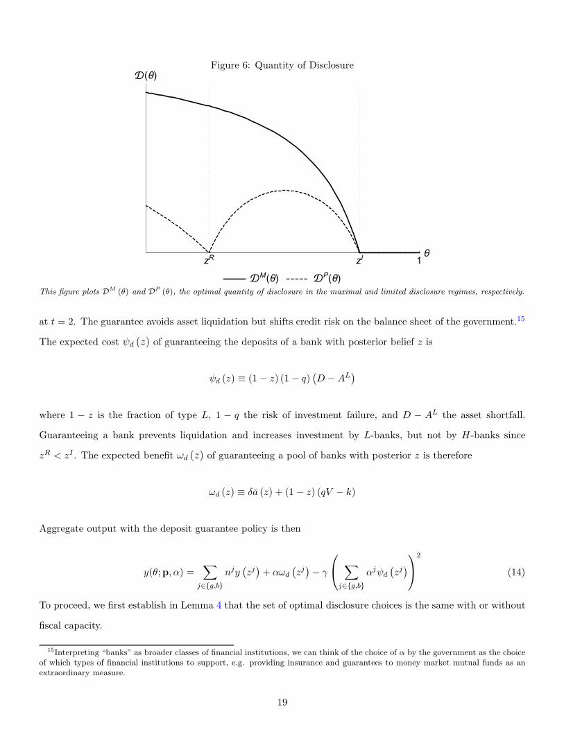
Figure 6: Quantity of Disclosure

zR zI 1θ

(θ)

M(θ) P(θ)This figure plots DM (θ) and DP (θ), the optimal quantity of disclosure in the maximal and limited disclosure regimes, respectively.

at t = 2. The guarantee avoids asset liquidation but shifts credit risk on the balance sheet of the government.15

The expected cost ψd (z) of guaranteeing the deposits of a bank with posterior belief z is

ψd (z) ≡ (1− z) (1− q)(

D −AL)

where 1 − z is the fraction of type L, 1 − q the risk of investment failure, and D − AL the asset shortfall.

Guaranteeing a bank prevents liquidation and increases investment by L-banks, but not by H-banks since

zR < zI . The expected benefit ωd (z) of guaranteeing a pool of banks with posterior z is therefore

ωd (z) ≡ δa (z) + (1− z) (qV − k)

Aggregate output with the deposit guarantee policy is then

y(θ;p,α) =∑

j∈g,b

njy(

zj)

+ αωd

(

zj)

− γ

⎛

⎝

∑

j∈g,b

αjψd

(

zj)

⎞

⎠

2

(14)

To proceed, we first establish in Lemma 4 that the set of optimal disclosure choices is the same with or without

fiscal capacity.

15Interpreting “banks” as broader classes of financial institutions, we can think of the choice of α by the government as the choiceof which types of financial institutions to support, e.g. providing insurance and guarantees to money market mutual funds as anextraordinary measure.

19

Lemma 4. Optimal disclosure with deposit insurance is either limited or maximal.

Proof. See Appendix A

Lemma 4 implies that only L-bank deposits are ever guaranteed, since the only optimal posterior belief at

which runs occur is zb = 0. The cost and benefit of deposit insurance therefore simplify to ψd ≡ (1− q)(

D −AL)

and ωd ≡ δAL + qV − k, respectively. Substituting these values into (14), taking the derivative with respect to

αb and solving for the optimal policy gives optimal deposit insurance policy as αg = 0 and

αb = min(

nb,α∗)

,

where α∗ = ωd

2γψ2d.

Our next task is to characterize when it is optimal for a government to switch from limited to maximal

disclosure. Corollary 1 shows that maximal disclosure is optimal even without insurance when condition (12) is

satisfied. When condition (12) is not satisfied, limited disclosure is optimal in the absence of deposit insurance.

The following lemma shows the existence of a threshold value θ above which it is optimal to choose maximal

disclosure, and show that θ increases with γ.

Lemma 5. There exists a θ ∈(

0, zI)

such that maximal disclosure is optimal if and only if θ > θ. Furthermore,

θ is increasing in γ, ∂θ∂γ ≥ 0.

Proof. See Appendix A.

We can finally state our main result, that fiscal capacity increases disclosure.

Proposition 3. Optimal disclosure is increasing in fiscal capacity: ∂D∗(θ)∂γ ≤ 0.

Proof. Lemma 5 establishes the existence of a threshold value θ above which disclosure is maximal and below

which it is limited. This threshold is decreasing in fiscal capacity. As shown above, DM (θ) > DP (θ) for all

θ ∈(

0, zI)

. As γ decreases, disclosure jumps from limited to maximal for a set of θ to the left of the threshold

θ, and is unchanged at all other points. It follows that ∂D∗(θ)∂γ ≤ 0.

Figure 7 illustrates Proposition 3. The red dash-dotted (blue dashed) line is the optimal quantity of disclosure

in the maximal (limited) regime. The solid black line is the optimal quantity of disclosure with deposit insurance.

Given a fiscal cost parameter γ, there is a threshold θ ∈(

0, zI)

at which the optimal disclosure policy switches

from limited to maximal. Optimal disclosure is limited below θ and maximal above θ. The signal precisions

20

Figure 7: Quantity of Disclosure with Deposit Insurance

zR zIθ˜

1θ

( )Low Fiscal Capacity (High )

P( ) M( ) *( )

zR zI˜

1

( )High Fiscal Capacity (Low )

P( ) M( ) *( )This figure shows the optimal quantity of disclosure with deposit insurance for two different values of fiscal capacity γ. The reddashed dotted (blue dashed) line is the optimal quantity of disclosure in the maximal (limited) disclosure regime. The solid black lineis the optimal quantity of disclosure with deposit insurance, which is the same as under limited disclosure for θ < θ and the same asmaximal disclosure for θ > θ. The threshold at which disclosure jumps from limited to maximal is increasing in γ. The left panelof the figure shows a case in which γ is high (fiscal capacity is low) and θ is high. As fiscal capacity increases, θdecreases and thegovernment follows maximal disclosure for a larger range of values of θ, as in the right panel.

pg, pb

and quantity of disclosure D∗ are discontinuous at the threshold θ. The left panel shows the case of

low fiscal capacity (high γ). The right panel shows the case of high fiscal capacity (low γ). The threshold θ is

lower in the right panel, and therefore disclosure is everywhere (weakly) higher.

21

4 Aggregate Risk and the Paradox of Fiscal Capacity

In this section we study the consequences of aggregate risk for disclosure and fiscal interventions. The main

motivation is empirical relevance. The assumption that the regulator knows θ when designing the asset quality

review yields clean theoretical insights, but it is also widely counter-factual. Policy makers do not know what

results will come out of the tests, especially when the tests are undertaken during a financial crisis, as we model

in this paper.16 This risk often explains the reluctance of policy makers to commit to aggressive stress tests.

We therefore assume that the government does not know θ when it chooses its disclosure policy. It only knows

that θ is drawn from some distribution function π(θ) with support [θ, θ].

Our second departure from the analysis of Section 3 is to extend the range of fiscal interventions. Guarantees

on runnable claims (which we call deposit insurance for short) are only one of the tools used by governments

during financial crises. Other interventions involve discount lending, credit guarantees, and capital injections,

which are all essentially meant to foster new credit. These interventions have been recently analyzed by

Philippon and Skreta (2012) and Tirole (2012). They are particularly interesting in the context of our paper

because they interact differently with disclosure than deposit insurance does. As a result, we will be able a

new and unexpected insight: when the planner is risk averse, the expected size of the fiscal intervention can be

decreasing in fiscal capacity. We call this result the Paradox of Fiscal Capacity.

4.1 Aggregate Risk

The government needs to choose signal precision p without knowing the fraction of H-banks, θ. All agents share

a common prior belief about the distribution of θ, with probability density π (θ). The government’s problem

departs significantly from the Bayesian Persuasion framework and quickly becomes intractable. For tractability

we restrict disclosure technology such that pg = 1 as in the left panel of Figure 5. All H-banks receive good

signals, and we let p ≡ pb be the one-dimensional control variable for the planner.17 Given that H-types are

always correctly identified, we have

nb = p (1− θ) ,

16During a crisis, the main risk is clearly that of runs on weaker institutions. The design of stress tests in normal times involvesdifferent tradeoffs, such as learning and regulatory arbitrage.

17The important point about this information structure is that it avoids type I errors. A strong bank is never classified as weak,but a weak bank can pass as strong. This information structure is both realistic and theoretically appealing. It is realistic in thecontext of banking stress tests since problems actually uncovered by regulators are almost certainly there, and the main issue is toknow which problems have been missed. One theoretical appeal is that it corresponds to the smooth case of Figure 5 so we do notneed to deal with discontinuities in addition to risk. Another theoretical appeal is that this class of signal has the property thatdisclosure always (weakly) improves welfare in a pure adverse selection model. The general case is treated in Faria-e-Castro et al.(2015).

22

and ng = θ + (1− p) (1− θ). Agents know p and observe nb, therefore they also learn the aggregate state θ

when the test results are released. The posteriors for individual banks are zb = 0, and

zg =θ

θ + (1− p) (1− θ)≡ z (θ; p) .

Note that the posterior belief depends both on the precision p and on the realization of the aggregate state θ. In

Appendix B, we show that, under certain regularity conditions on π (θ), our previous result regarding deposit

insurance continues to hold: a planner with a strong fiscal position discloses more than a planner with a weak

position. The special case where θ ∈[

zR, zI]

is particularly relevant because it corresponds to the case where

the markets are frozen.18 In that case, we can show that ex-ante disclosure decreases with γ.

4.2 Credit Guarantees

Let us now consider government interventions at at time 1. Adverse selection in credit markets leads to ineffi-

ciently low investment and provides room for welfare-improving policies. We know from Philippon and Skreta

(2012) that the optimal policy takes the form of a credit guarantee. Such guarantees were provided by the

FDIC and by most European governments in 2009 and 2010.

In our setup, this policy is only relevant for the pool of banks that receive a good signal at time 0 since

banks with bad signals are all of same type (L). We use the following results from Philippon and Skreta (2012)

and Tirole (2012):

Proposition 4. Direct lending by the government, or the provision of guarantees on privately issued debts, are

constrained efficient. The cost of any optimal intervention is equal to the rents of informed agents.

Proof. See Philippon and Skreta (2012).

The proposition states that if the government chooses to intervene, it should either lend directly to banks

or provide guarantees on new debts, as opposed to buying assets, injecting capital, etc. The optimal policy

consists of lending at the rate rH from equation (8), the highest rate at which banks of type H are willing to

invest. Setting the rate above rH is ineffective, and setting it below rH offers an unnecessary subsidy. The

benefit per loan from such a program is

ωa (z) = 1z∈[zR,zI ] · z(qV − k)

18It is also rather tractable because only banks with the low signal (may) receive deposit insurance and only banks with the highsignal (may) receive credit guarantees.

23

The proposition also says that there is a minimum cost for any intervention, i.e. it it not possible to unfreeze

credit markets for free. Proving this result is difficult because the space of interventions is large, but the

intuition is rather clear. Bad banks can always mimic good banks and these informational rents are always paid

in equilibrium. In the context of our model, the profit per loan k for the government is

z(rH − 1)k + (1− z)(qrH − 1)k = z(qV − k) + (1− z)(q2V − k)

The best the government can do is to extract the surplus from the good bank. The informational rent is capture

by the extra q term in the second term. It is easy to see that this profit is strictly negative as long as z < zI .

The government also needs to decide the size of the intervention, measured by the number of banks β that

benefit from the program. The total cost of the credit guarantee program is

Ψa (β; z) = β k − qV [z (1− q) + q] ≡ βψa (z) . (15)

Finally, output with credit guarantees β is

y (θ;p,β) = nby (0) + ngy (zg) + βωa (zg)− γ [βψa (z

g)]2 . (16)

Note that the benefit is increasing in z (up to z ≤ zI), while the costs are decreasing in z. Since the intervention

occurs after the stress test, the government takes the fraction of strong banks θ and the precision of the signal

p as given when choosing the size of the intervention, solving the following program

maxβ∈[0,ng(θ;p)]

y (θ;p,β) ,

and we get the following result.

Lemma 6. The optimal number of credit guarantees is given by

β = min

ng (θ; p) ,ωa(θ; p)

2γψa(θ; p)2

for z (θ; p) < zI and β = 0 otherwise.

Note that, taking as given the other interventions, the size of the program decreases with γ. We will see

that this result is overturned when we solve jointly for the various policies.

The full analysis of disclosure and fiscal policy involves the solution to a relatively complex program with

24

Figure 8: Optimal Disclosure with Deposit Insurance and Credit Guarantees

0 5 10 150

0.5

1

p∗, Optimal Disclosure

γ

pm

0 5 10 150

0.25

E[Ψ], Expected Support

γ

Deposit InsuranceCredit Guarantee

This figure plots optimal disclosure and expected fiscal spending as a function of γ, the measure of fiscal capacity. The leftpanel plots p∗, the optimal disclosure policy. The right panel plots expected spending, broken down by type.

three dimensions of intervention and one dimension of risk. Due to the complexity of this problem, we proceed

numerically to study how the optimal choice of disclosure changes with γ. The left panel of Figure 8 depicts

this comparative static, for θ ∼ U[

zR, zI]

. Optimal disclosure is (weakly) decreasing in γ as in our baseline

result: high fiscal capacity translates into greater ability to provide credit and deposit guarantees - to “mop

up” in case a bad state of the world materializes, leading the government to choose high levels of disclosure. As

γ increases, and fiscal capacity becomes more limited, the government opts for intermediate levels of disclosure,

eventually choosing no disclosure (p = 0) for γ high enough.

The right panel of Figure 8 plots expected government spending Eθ [Ψ] by type of intervention. For low

levels of γ, the planner chooses high disclosure, unfreezing markets and creating runs. It relies on deposit

guarantees but not on credit guarantees. The logic is reversed when γ increases. As of disclosure decreases, the

planner no longer needs to offer deposit guarantees, but increases spending on credit guarantees.

An interesting result that arises from our analysis is therefore that a less fiscally constrained planner, by

disclosing more, reduces the need to offer credit guarantees. In the next section, we show that this effect is

magnified when the planner is risk-averse.

25

4.3 Risk-Aversion and the Paradox of Fiscal Capacity

Consider finally the case where the planner is risk-averse. Letting y(θ;p,α,β) denote the state-contingent level

of consumption in the final period, the planner now solves the following problem:

maxp∈[0,1]

Eθ

[

maxα,β

u (y (θ;p,α,β))

]

,

subject to feasibility constraints on (α,β). We consider the case of power utility, u(c) = y1−σ

1−σ , where σ is the

coefficient of relative risk-aversion. We show that making the planner risk-averse delivers the additional insight

that increased fiscal capacity may be associated with lower expected spending. We call this the paradox of

fiscal capacity. It relies on both risk-aversion and the fact that disclosure and ex-post guarantees are strategic

substitutes.

We plot an instance of this comparative static in Figure 9. For this figure, we assumed that θ follows a two

point distribution, with equal probability in each mass point. When fiscal capacity is high, the planner chooses

to fully unfreeze the credit markets and to use its fiscal capacity to limit runs.19

Beyond a certain level of γ, however, the planner chooses to set p∗ = 0 because the planner does not have

the capacity to deal with runs in the bad state of the world. The planner chooses instead to offer guarantees.

The interesting point is that this policy is actually more expensive than the previous one, as the second panel

shows. The reason for this is that while the average cost of deposit insurance is lower, it has a greater downside

risk. To avoid this risk, the planner prefers to incur the higher average cost of low disclosure and guarantees.

19Given the restrictions we consider on the distribution, we show in the appendix that full disclosure does not necessarily implythat p = 1. Rather, we derive a minimum level of disclosure pm at which the planner is able to unfreeze markets with probabilityone, which we call full disclosure, and show that it is never optimal to exceed this level.

26

Figure 9: Paradox of Fiscal Capacity

0 2 4 6

γ

0

0.2

0.4

0.6

0.8

p∗, Optimal Disclosure

0 2 4 6

γ

0

0.05

0.1

0.15

Expected Spending

0 2 4 6

γ

0

0.05

0.1

0.15

Expected Support

DepositCredit

This figure presents the paradox of fiscal capacity. We assume that σ = 10 and that θ is distributed with equal probabilityon two mass points: θ = 0.8zR + 0.2zI and θ = 0.2zR + 0.8zI.

27

5 Discussion and Conclusion

We have provided a first analysis of the interaction between fiscal capacity and disclosure during financial crises.

We identify a fundamental trade-off for optimal disclosure. To reduce adverse selection it is often optimal to

increase the variance of investors’ posterior beliefs. To avoid runs, on the contrary, it is often optimal not to

increase posterior variance. Fiscal capacity improves this trade-off because it gives the government the flexibility

to deal with runs if they occur. Disclosure and deposit insurance are strategic complements and a government

is more willing to disclose information when its fiscal position is strong. We argue that these predictions are

consistent with government actions in Europe and in the United States during the recent financial crisis.

On the other hand, aggressive disclosure can restore efficiency in private credit markets and make other

forms of bailouts (credit guarantees, asset purchases, or capital injections) unnecessary. As a result, and

somewhat paradoxically, fiscally constrained governments, who are worried about the risk of disclosure, can end

up spending more on bailouts.

There are several potentially interesting extensions to our analysis. One would be to consider endogenous

information acquisition by lenders, as in Hellwig and Veldkamp (2009). The nature of runs versus lemons can

generate conflicting incentives for agents who are both depositors and creditors. On the one hand, they are

strategic complements when it comes to runs, since a depositor would like to know who else intends to run when

deciding to run or not. On the other hand, they are strategic substitutes in credit markets, since a creditor

would like to be the only one to know that a particular bank is good.

Another important feature of our model is that government’s actions do not have a signaling content. This

is different from the models of Angeletos et al. (2006) and Angeletos et al. (2007). In our model the government

and the private lenders share the same information set about the aggregate state.

Finally the point that fiscal flexibility increases disclosure has important implications for recent regulatory

initiatives aimed at limiting bailouts by reducing policy discretion. Restricting fiscal flexibility may lead the

government to disclose less and provide more support in credit markets instead.

28

References

Akerlof, G. A. (1970): “The Market for ‘Lemons’: Quality Uncertainty and the Market Mechanisms,”

Quarterly Journal of Economics, 84, 488–500. (document)

Allen, F. and D. Gale (2000): “Financial Contagion,” Journal of Political Economy, 108, 1–33. (document)

Alvarez, F. and G. Barlevy (2015): “Mandatory Disclosure and Financial Contagion,” NBER Working

Papers 21328, National Bureau of Economic Research, Inc. (document)

Angeletos, G.-M., C. Hellwig, and A. Pavan (2006): “Signaling in a Global Game: Coordination and

Policy Traps,” Journal of Political Economy, 114, 452–484. (document), 5

——— (2007): “Dynamic Global Games of Regime Change: Learning, Multiplicity, and the Timing of Attacks,”

Econometrica, 75, 711–756. 5

Bouvard, M., P. Chaigneau, and A. de Motta (2015): “Transparency in the Financial System: Rollover

Risk and Crises,” Journal of Finance, 70, 1805–1837. (document)

Carlsson, H. and E. van Damme (1993): “Global Games and Equilibrium Selection,” Econometrica, 61,

989–1018. (document)

Chari, V. and P. J. Kehoe (2013): “Bailouts, Time Inconsistency, and Optimal Regulation,” NBER Working

Papers 19192, National Bureau of Economic Research, Inc. (document)

Chari, V. V., A. Shourideh, and A. Zetlin-Jones (2014): “Reputation and Persistence of Adverse

Selection in Secondary Loan Markets,” American Economic Review, 104, 4027–70. (document)

Diamond, D. W. (2001): “Should Japanese Banks Be Recapitalized?” Monetary and Economic Studies, 1–20.

(document)

Diamond, D. W. and P. H. Dybvig (1983): “Bank Runs, Deposit Insurance, and Liquidity,” Journal of

Political Economy, 91, 401–419. (document)

Diamond, D. W. and R. G. Rajan (2011): “Fear of Fire Sales, Illiquidity Seeking, and Credit Freezes,”

Quarterly Journal of Economics, 126, 557–591. (document)

Faria-e-Castro, M., J. Martinez, and T. Philippon (2015): “A Note on Information Disclosure and

Adverse Selection,” Mimeo, New York University. 17

29

Goldstein, I. and Y. Leitner (2013): “Stress tests and information disclosure,” Working Papers 13-26,

Federal Reserve Bank of Philadelphia. (document)

Goldstein, I. and H. Sapra (2014): “Should Banks’ Stress Test Results be Disclosed? An Analysis of the

Costs and Benefits,” Foundations and Trends(R) in Finance, 8, 1–54. (document)

Gorton, G. (1985): “Bank suspension of convertibility,” Journal of Monetary Economics, 15, 177 – 193. 9

——— (2012): Misunderstanding Financial Crises: Why We Don’t See Them Coming, Oxford University Press,

Oxford, UK. (document)

Gorton, G. and L. Huang (2004): “Liquidity, Efficiency, and Bank Bailouts,” American Economic Review,

94, 455–483. (document)

Gorton, G. and A. Metrick (2012): “Securitized banking and the run on repo,” Journal of Financial

Economics, 104, 425–451. (document)

Gorton, G. and G. Ordonez (2014): “Collateral Crises,” American Economic Review, 104, 343–378.

(document)

He, Z. and W. Xiong (2012): “Rollover Risk and Credit Risk,” Journal of Finance, 67, 391–430. (document)

Heider, F., M. Hoerova, and C. Holthausen (2010): “Liquidity Hoarding and Interbank Market Spreads:

The Role of Counterparty Risk,” CEPR Discussion Papers 7762, C.E.P.R. Discussion Papers. 2.4

Hellwig, C. and L. Veldkamp (2009): “Knowing What Others Know: Coordination Motives in Information

Acquisition,” Review of Economic Studies, 76, 223–251. (document), 5

Hirshleifer, J. (1971): “The Private and Social Value of Information and the Reward to Inventive Activity,”

American Economic Review, 61, pp. 561–574. (document)

Kamenica, E. and M. Gentzkow (2011): “Bayesian Persuasion,” American Economic Review, 101, 2590–

2615. (document), 3.1, 3.1, 3.2

Kareken, J. H. and N. Wallace (1978): “Deposit Insurance and Bank Regulation: A Partial-Equilibrium

Exposition,” Journal of Business, 413–38. (document)

Landier, A. and K. Ueda (2009): “The Economics of Bank Restructuring; Understanding the Options,”

IMF Staff Position Notes 2009/12, International Monetary Fund. (document)

30

Mitchell, J. (2001): “Bad Debts and the Cleaning of Banks’ Balance Sheets: An Application to Transition

Economies,” Journal of Financial Intermediation, 10, 1–27. (document)

Morris, S. and H. S. Shin (2000): “Rethinking Multiple Equilibria in Macroeconomic Modeling,” in NBER

Macroeconomic Annual Macroeconomic Annual, ed. by B. S. Bernanke and K. Rogoff, vol. 15, 139–161.

(document)

Myers, S. C. and N. S. Majluf (1984): “Corporate Financing and Investment Decisions when Firms Have

Information that Investors do not have,” Journal of Financial Economics, 13, 187–221. (document)

Nachman, D. and T. Noe (1994): “Optimal Design of Securities under Asymmetric Information,” Review of

Financial Studies, 7, 1–44. (document), 2.3

Ong, L. L. and C. Pazarbasioglu (2014): “Credibility and Crisis Stress Testing,” International Journal of

Financial Studies, 2, 15–81. 1

Parlatore, C. (2013): “Transparency and Bank Runs,” New York University Stern School of Business.

(document)

Philippon, T. and P. Schnabl (2013): “Efficient Recapitalization,” Journal of Finance, 68, 1–42. 2,

(document), 11

Philippon, T. and V. Skreta (2012): “Optimal Interventions in Markets with Adverse Selection,” American

Economic Review, 102, 1–28. (document), 1.1, 6, 2.3, 4, 4.2, 4.2

Shapiro, J. and D. Skeie (2015): “Information Management in Banking Crises,” Review of Financial Studies,

28, 2322–2363. (document)

Tirole, J. (2012): “Overcoming Adverse Selection: How Public Intervention Can Restore Market Functioning,”

American Economic Review, 102, 29–59. (document), 6, 4, 4.2

Uhlig, H. (2010): “A model of a systemic bank run,” Journal of Monetary Economics, 57, 78–96. (document)

Veron, N. (2012): “The challenges of Europe’s fourfold union,” Policy Contributions 741, Bruegel. 1

Williams, B. (2015): “Stress Tests and Bank Portfolio Choice,” . 2, (document)

Zetlin-Jones, A. (2014): “Efficient Financial Crises,” GSIA Working Papers 2014-E19, Carnegie Mellon

University, Tepper School of Business. 2, (document)

31

A Proofs

Proof of Lemma 4 Notice first that there is no point in setting zg < zR and we only need to consider policies

with zg ≥ zR. When θ < zR, it is also always optimal to set zb = 0 because this increases ng without affecting

the cost of runs. Any disclosure choice such that zg ∈(

zR, zI)

has strictly lower payoff than

zb, zg

=

0, zR

,

because it requires more runs and provides no benefit. It follows that for θ ∈(

0, zR)

, zb = 0 and zg ∈

zR, zI

.

By analogous arguments, for θ ∈(

zR, zI)

, zg = zI and zb ∈

0, zR

. For θ ≥ zI , there is no disclosure since

first best output is attained.

Proof of Lemma 5 We prove the Lemma by directly characterizing the properties of the cutoff θ. Another

(indirect) strategy to prove the comparative statics result would rely on the super-modularity of the objective

function and then show that there is a monotonic relation between spending and disclosure. We present the

direct proof because it allows us to also discuss the nature of the optimal disclosure. Corollary 1 shows that

maximal disclosure is optimal even without insurance when condition (12) is satisfied. In this case, we simply

have θ = 0. When condition (12) is not satisfied, limited disclosure is optimal in the absence of deposit

insurance. When θ ∈(

0, zR)

, the government makes use of deposit insurance under both disclosure regimes.

The government is indifferent between limited and maximal disclosure when

θ

zR(

AHzR +AL(

1− zR)

+ qV − k)

+

(

1−θ

zR

)

(1− δ)AL + αbP

(

δAL + qV − k)

− γ(

ψαbP

)2=

θ

zI(

AHzI +AL(

1− zI)

+ qV − k)

+

(

1−θ

zI

)

(1− δ)AL + αbM

(

δAL + qV − k)

− γ(

ψαbM

)2(17)

Where αbP = min

(

1− θzR

,α∗)

is the optimal deposit insurance policy with limited disclosure and αbM =

min(

1− θzI,α∗

)

with maximal disclosure. We show first that any solution θ to (17) must be such that

αbP = 1 − θ

zRand αb

M = 1 − θzI. Since α∗ > 1 − θ

zI> 1 − θ

zI, this implies θ > (1− α∗) zI . The LHS and

the RHS are increasing in θ and equal at θ = 0. Further, the slope of the LHS in θ is greater than that of the

RHS for θ < (1− α∗) zI as long as inequality (12) is not satisfied. It follows thatθ > (1− α∗) zI . Substituting

αbP = 1− θ

zRand αb

M = 1− θzI

into (17) gives a quadratic in θ, with roots θ = 0 and

θ =zIzR

zI + zR

(

2−(qV − k) zIzR

γψ2 (zI − zR)

)

(18)

32

It is easily verified that ∂θ∂γ > 0 so the maximal disclosure threshold is decreasing in fiscal capacity (increasing

in γ).

We now solve for the value of θ ∈(

zR, zI)

at which the planner is indifferent between limited disclosure

and maximal disclosure with deposit insurance. Note that for θ ∈(

zR, zI)

, limited disclosure doesn’t cause

runs and therefore does not result in the use of deposit insurance. Equating welfare with limited disclosure (the

LHS) and welfare with full disclosure and deposit insurance:

θ − zR

zI − zR(

AHzI +AL(

1− zI)

+ qV − k)

+zI − θ

zI − zR(

AHzR +(

1− zR) (

AL + qV − k))

=θ

zI(

AHzI +AL(

1− zI)

+ qV − k)

+

(

1−θ

zI

)

(1 − δ)AL + αb(

δAL + qV − k)

− γ(

ψαb)2

(19)

After maximal disclosure, nb = 1 − θzI, so αb = min

(

1− θzI,α∗

)

, and there are two cases to consider.

Denoting by θ the solution to (19), either zR < θ < zI (1− α∗) and αb = α∗, or θ ≥ zI (1− α∗) and αb = 1− θzI.

Substituting in αb = nb = 1− θzI

gives a quadratic in θ, the roots of which are θ = zI and

θ = zI(

1−(qV − k)zIzR

γψ2 (zI − zR)

)

(20)

∂θ∂γ > 0 so again the maximal disclosure threshold is decreasing in fiscal capacity (increasing in γ). For this to

be a solution, it must be that min(

1− θzI,α∗

)

= 1− θzI, or θ > zI (1− α∗). Substituting in for θ and α∗, this

reduces to zR−zI(1−zR)(zI−zR) qV −k < δAL, which is the converse of the condition derived in Corollary 1. The solution

is therefore valid as long as maximal disclosure is not optimal in the absence of deposit insurance, which is the

case we are interested in. It is easily verified that the RHS of 19 exceeds the LHS for θ > θ .

To establish that maximal disclosure is optimal for θ > θ for θ ∈(

0, zI)

it suffices to show that the θ > θ,

or zI(

1− (qV−k)zIzR

γψ2(zI−zR)

)

≥ zIzR

zI+zR

(

2− (qV−k)zIzR

γψ2(zI−zR)

)

. This inequality reduces to θ ≥ zR. It follows that maximal

disclosure is optimal for θ > θ, with

θ =

⎧

⎪

⎪

⎨

⎪

⎪

⎩

max(

0, zIzR

zI+zR

(

2− (qV−k)zIzR

γψ2(zI−zR)

))

if zI(

1− (qV−k)zIzR

γψ2(zI−zR)

)

< zR

zI(

1− (qV−k)zIzR

γψ2(zI−zR)

)

otherwise

33

B Optimal Disclosure with Aggregate Risk

In this appendix, we present a series of results for our baseline model with aggregate risk. By imposing

the restriction on the disclosure technology that we consider in Section 4 as well as additional restrictions

on the planner’s preferences and the distribution for the aggregate state, we are able to establish several

results regarding the endogenous choice of disclosure, as well as the interaction between this choice and fiscal

interventions. In this version of the model, the government chooses the precision of the signals received by each

bank at the beginning of period 0, before it knows the realization of the aggregate state θ. We assume that

the government shares with private agents a common prior belief about the distribution of the aggregate state,

π (θ).

Additionally, to make our analysis tractable, we deviate from the model presented in the main text along

two dimensions:

1. Preferences are linear in aggregate output, u [y (θ)] = y (θ)

2. The distribution for the aggregate state has bounded support, π (θ) ⊂[

θ, θ]

=[

zR, zI]

After the realization of the aggregate state and of the signal for each bank, agents form posterior probabilities of

each bank being of typeH, as explained in the main text. Since zR > 0, banks that receive the bad signal always

suffer runs. Banks that receive the good signal may or may not suffer runs depending on how z1 compares to

zR. The case z1 < zR is not very interesting since it implies a full, unconditional run. To sharpen our analysis,

we assume that a small set of agents observes the aggregate state θ at the beginning of period 0. With this

refinement, if the aggregate state is such that θ < zR then an aggregate run occurs immediately. The informed

agents run, and all other depositors observe the run and run as well. A run on the entire system obviously

renders stress tests and asset quality reviews useless. In such a scenario, the government would simply try to

save banks by issuing guarantees, as discussed later. This is not a very interesting scenario and the refinement

allows us to separate this extreme case from more interesting, intermediate ones.20

Conditional on no immediate run all agents know that θ ≥ zR, and since z1 > θ there is no run on banks

that receive good signals. We can then think of π (θ) as the distribution of θ conditional on no aggregate run

being observed.21 At the other extreme, the case θ > zI does not change our findings but requires additional

notation, so we remove this possibility as well.22

20To wit, in the aftermath of the financial crisis, even countries with deeply troubled banking systems such as Cyprus did notexperience such unconditional runs.

21Formally, let the primitive distribution of θ be denoted by π0 (θ). Our analysis focuses on the distribution that arises conditional

on θ ≥ zR, which we call π (θ) ≡π0(θ|θ≥zR)1−Π0(zR)

for simplicity.22The set-up for the general model is presented in Appendix E.

34

Figure 10: Equilibrium Regions

0 0.2 0.4 0.6 0.8 1

0.3

0.35

0.4

0.45

0.5

0.55

0.6

0.65

0.7

p

θ AdverseSelection

EfficientθI(p)

zI

zR

This figure illustrates the equilibrium regions in (p, θ) space. The line is the investment threshold, θI (p).

We therefore focus on the case [θ, θ] = [zR, zI ]. The equilibrium with stress testing is then characterized by

the number of banks in each category, n0 and n1, and by the comparison between z1 (θ, p) and zI .23 For banks

with good signals, there are two possible outcomes, depending on the values of θ and p.

1. Banks with the good signal face adverse selection, zR ≤ z1 (θ, p) < zI ;

2. All banks with the good signal invest, zI ≤ z1 (θ, p).

We can characterize the equilibrium outcome for banks that receive the good signal for any pair (θ, p) using a

threshold on θ: the minimum realization of the aggregate state for which all banks that receive the good signal

invest

θI (p) = min

θ | z (θ, p) ≥ zI

(21)

The power of the stress test p determines this threshold, against which the realization of θ is compared to

determine the equilibrium outcome. This threshold, and the possible equilibrium regions, are depicted in

Figure B for θ ∈[

zR, zI]

and p ∈ [0, 1].

For the economy with stress testing, welfare is given by (11). The sets of liquidated banks and banks that

23Most results we derive from this point onwards are also valid for the case where [θ, θ] ⊂ [zR, zI ], at the expense of minoradjustments and extra notation.

35

choose not to invest are given by

Λ (θ, p) =p (1− θ)

Ω (θ, p) =1z(θ,p)<zI · θ

This results in the following expression for welfare in the decentralized equilibrium, given (θ, p)

y (θ; p,∅) = y (θ)− p (1− θ)(

δAb + qV − k)

− 1z(θ,p)<zI · θ (qV − k) (22)

The first term is first-best welfare; the second term corresponds to losses due to liquidation and foregone

investment by banks that suffer runs; the final term is foregone investment due to adverse selection. Note that

the last term is only positive when z (θ, p) < zI , or θ < θI (p). Taking expectations over θ, expected welfare

can be written as

Eθ [y (θ; p,∅)] = Eθ [y (θ)]− pEθ [1− θ](

δAb + qV − k)

− (qV − k)

ˆ θI(p)

zRθdΠ (θ) (23)

where Π (θ) =´ θθ π (x) dx is the cumulative distribution function of θ.

The government’s disclosure problem, before the aggregate state θ is realized, can then be formulated as

maxp∈[0,1]

Eθ [y (θ; p,∅)] (24)

By increasing the informativeness of its disclosure policy, the government raises (in expectation) the perceived

quality z1 of banks that receive the good signal, thereby increasing expected investment by strong banks. This

comes at the cost of revealing some banks to be weak and therefore causing runs (recall that banks that receive

the bad signal are run with certainty). The government effectively trades off the (expected) sizes of the sets

Λ (θ, p) and Ω (θ, p).

To further develop intuition about the costs and benefits of disclosure, Lemmas 7 and 8 provide results on

optimal disclosure in the absence of runs and lemons, respectively.

Lemma 7. If there are no runs, welfare is weakly increasing in p (strictly increasing if θI (p) > zR), and full

disclosure is optimal.

36

Proof. Without runs, welfare can be written as

Eθ [y (θ; p,∅)] = Eθ [θ]Ag + Eθ [1− θ]

(

Ab + qV − k)

+

ˆ θ

θI(p)θ (qV − k) dΠ (θ)

The derivative of welfare with respect to p is

dEθ [y (θ; p,∅)]

dp= 1θI (p)≥θ · π

[

θI (p)]

θI (p) (qV − k)

[

−dθI (p)

dp

]

≥ 0

It is strictly positive for p : θI (p) ≥ θ, and zero otherwise. Welfare is strictly increasing in p for p ≤ pm, and

constant afterwards. Full disclosure is then (weakly) optimal.

In the absence of runs, welfare is strictly increasing in p starting from zero disclosure: disclosing information

increases the average quality of banks with the good signal, decreasing the probability that credit markets will

be affected by adverse selection.24 Beyond a certain level of p, which we denote by pm, the average quality of

banks with the good signal is high enough that they all invest with certainty in every state of the world, even

for very low realizations of θ. Increasing p yields no further benefits, so in the absence of runs the planner is

indifferent between disclosure choices in [pm, 1].

pm : θI (pm) = zR ⇒ pm =zI − zR

zI (1− zR)∈ (0, 1)

Lemma 8. If there is no adverse selection, welfare is strictly decreasing in p and zero disclosure is optimal.

Proof. Without adverse selection, expected welfare can be written as

Eθ [y (θ; p,∅)] = pEθ [1− θ] (1− δ)Ab + Eθ [θ] (Ag + qV − k) + (1− p)Eθ [1− θ]

(

Ab + qV − k)

The derivative with respect to p is

dEθ [y (θ; p,∅)]

dp= −Eθ [1− θ]

[

δAb + qV − k]

< 0

strictly negative for p ∈ [0, 1]. Therefore, p = 0 is optimal.

Absent adverse selection, the only effect of disclosure is that banks that are revealed to be weak suffer runs.

24This is not a general property of information disclosure in an adverse selection setting. For example, if the asymmetricinformation pooling equilibrium is such that investment is efficient, disclosing the identity of strong banks weakly decreases welfare,since it reduces the likelihood that the pooling equilibrium will induce efficient investment. A previous version of our modelconsidered this possibility. Our chosen form of disclosure technology is both more realistic and analytically tractable.

37

Figure 11: Expected mass at Λ and Ω, θ ∼ U[

zR, zI]

0 0.2 0.4 0.6 0.8 1

p

0

0.1

0.2

0.3

0.4

0.5

0.6

0.7

0.8

0.9

1

pm

Banks in Λ

Banks in Ω

This figure plots the expected mass of banks in the set Ω (banks that opt out of credit markets due to adverse selection) and theset Λ (banks that suffer a run and liquidate assets) as a function of p, assuming a uniform distribution of the aggregate state,π (θ) = U

[

zR, zI]

.

Figure B represents the trade-off graphically: it plots the expected mass of banks that are affected by adverse

selection, and the expected mass of banks that suffer runs, as a function of p. The mass of banks that are

expected to suffer a run is strictly increasing in p, as p = 1 corresponds to the extreme case in which the signal

is perfect and no weak bank receives the good signal. The mass of banks that are expected to suffer from

adverse selection is decreasing until pm, after which disclosure is high enough that the pool of banks with the

good signal invests efficiently even for low realizations of θ.

We proceed to characterize the problem with runs and lemons. We first establish that there exists an interior

upper bound on the amount of disclosure that the planner chooses.

Corollary 2. In the economy with runs and lemons, the planner never sets p > pm.

Proof. The derivative of expected welfare with respect to p is

dEθ [y (θ; p,∅)]

dp= 1θI(p)≥θ · π

[

θI (p)]

θI (p) (qV − k)

[

−dθI (p)

dp

]

− Eθ [1− θ][

δAb + qV − k]

The first term is only positive for p ≤ pm, while the second term is always negative. Thus welfare is strictly

decreasing for p > pm, and the planner sets at most p = pm.

This result follows immediately from the previous lemmas: increasing disclosure above pm offers no benefits

38

from unfreezing markets while still causing weak banks to suffer runs, so the planner will never choose a level

of disclosure beyond pm. We now characterize the solution to the disclosure problem in terms of the properties

of the distribution of the aggregate state. Proposition 5 describes the government’s optimal disclosure policy

for different characteristics of the distribution π (θ).

Proposition 5. Let

χ (θ) ≡ θπ′ (θ)

π (θ)

If χ (θ) ≥ 3zI−11−zI

,∀θ ∈[

zR, zI]

, welfare is a strictly concave function in [0, pm], and the optimal level of disclosure

solves the first-order condition

π[

θI (p)]

θI (p) (qV − k)

[

−dθI (p)

dp

]

− Eθ [1− θ][

δAb + qV − k]

= 0

If χ (θ) ≤ 3zR−11−zR

,∀θ ∈[

zR, zI]

, welfare is a strictly convex function in [0, pm]. The optimal level of disclosure

is p = 0 if and only if

pm(δAb + qV − k)

qV − k + pm(δAb + qV − k)≥ Eθ[θ] (25)

and is p = pm otherwise.

Proof. For any distribution π (θ), the derivative of expected welfare with respect to p is

dEθ [y (θ; p,∅)]

dp= 1θI(p)≥θ · π

[

θI (p)]

θI (p) (qV − k)

[

−dθI (p)

dp

]

− Eθ [1− θ][

δAb + qV − k]

We can write the second derivative of expected welfare with respect to p as

d2Eθ [y (θ; p,∅)]

dp2= −1θI(p)≥θ · (qV − k)π

[

θI (p)]

[

dθI (p)

dp

]2[

1 + θI (p)π′

[

θI (p)]

π [θI (p)]

]

+ θI (p)d2θI (p)

dp2

Replace for the derivatives of θI (p) and simplify to obtain

d2Eθ [y (θ; p,∅)]

dp2= 1θI(p)≥θ · (qV − k)π

[

θI (p)]

(

1/zI − 1)

(1/zI − p)4

3− 1/zI − χ[

θI (p)] (

1/zI − 1)

− 2p

(26)

Note that all the terms except for the last one are strictly positive for p ≤ pm. The shape of the welfare function is

therefore determined by the sign of this last term. For the welfare function to be strictly concave, we need this term to

39

be strictly negative for any p ∈ [0, pm]. This is equivalent to

3− 1/zI − χ[

θI (p)] (

1/zI − 1)

− 2p < 0

⇔χ[

θI (p)]

>3− 1/zI − 2p

1/zI − 1

Note that the right-hand side is strictly decreasing on p. It is then enough to show that

minp∈[0,pm]

χ[

θI (p)]

> maxp∈[0,pm]

3− 1/zI − 2p

1/zI − 1=

3zI − 1

1− zI

So that a sufficient (but not necessary) condition for this to be satisfied is to ensure that

χ (θ) >3zI − 1

1− zI, ∀θ ∈

[

θ, θ]

In this case, the expected welfare function is strictly concave on [0, pm], so the first-order condition is sufficient and

necessary for the optimum

dEθ [y (θ; p,∅)]

dp= π

[

θI (p)]

θI (p) (qV − k)

[

−dθI (p)

dp

]

− Eθ [1− θ][

δAb + qV − k]

= 0

Equivalently, we can establish a sufficient condition for convexity by ensuring that the last term of 26 is strictly positive.

This happens, whenever

χ[

θI (p)]

<3− 1/zI − 2p

1/zI − 1

It is enough to show that

maxp∈[0,pm]

χ[

θI (p)]

< minp∈[0,pm]

3− 1/zI − 2p

1/zI − 1=

3zR − 1

1− zR

A sufficient condition for this is to ensure that

χ (θ) <3zR − 1

1− zR, ∀θ ∈

[

zR, zI]

In this case, due to strict convexity of the welfare function, the optimum must be at one of the boundaries of the choice

set. These are 0 and pm. We can evaluate expected welfare at each of these points and compare the values

Eθ [y (θ; p,∅)]|p=0 = Eθ [θ]Ag + Eθ [1− θ]

(

Ab + qV − k)

Eθ [y (θ; p,∅)]|p=pm = Eθ [θ] (Ag + qV − k) + pmEθ [1− θ] (1− δ)Ab + (1− pm)Eθ [1− θ]

(

Ab + qV − k)

40

The planner prefers not to disclose, p = 0, if and only if

Eθ [y (θ; p,∅)]|p=0 ≥ Eθ [y (θ; p,∅)]|p=pm

pm ≥Eθ [θ]

Eθ [1− θ]

1

1 + δAb

qV −k

which is equivalent topm(δAb + qV − k)

qV − k + pm(δAb + qV − k)≥ Eθ[θ]

At an interior optimum in [0, pm] the planner equates the expected marginal cost and benefit of additional

disclosure, given by Eθ [1− θ][

δAb + qV − k]

and π[

θI (p)]

θI (p) (qV − k)[

−dθI (p)dp

]

respectively. Proposition

5 provides a sufficient condition for strict concavity of the welfare function (which is necessary for the existence

of an interior optimum). Since disclosure always causes runs, the expected marginal cost is constant and equal

to the expected mass of weak banks times the cost of a run (liquidation cost δAb plus the value of foregone

investment qV − k). The expected benefit from increased disclosure is a non-linear function of p: the planner is

not only uncertain about the number of strong banks, but also about the effect that additional disclosure has

on investment by strong banks.

If, on the other hand, χ(θ) is uniformly low enough such that welfare is convex in [0, pm], the planner sets

disclosure to either 0 or the maximum. The condition that determines which corner is chosen is intuitive: if

the expected cost of runs at the maximum level of disclosure (the mass of banks that is run, Eθ [1− θ], times

the cost of runs) exceeds the expected benefit of achieving full investment by strong banks, the planner chooses

p = 0. It follows that the lower the expected mass bank of strong banks, the less likely it is that full disclosure

is chosen. The following lemma allows us to establish that, when optimal disclosure is at a corner, decreasing

χ(θ) uniformly will never lead to more disclosure.

Lemma 9. For two distributions π1(θ) and π0(θ), if χ1(θ) > χ0(θ) ∀θ, then E1(θ) > E0(θ).

Proof. Let π0(θ) and π1(θ) be two probability density functions such that

θπ′1(θ)

π1(θ)> θ

π′0(θ)

π0(θ)∀θ

Canceling θ and integrating both sides from θ0 to θ1 > θ0 gives:

π1(θ1)

π1(θ0)>π0(θ1)

π0(θ0)

41

So χ1(θ) > χ0(θ) implies that π1(θ) likelihood ratio dominates π0(θ). It then follows that

E1(θ) > E

0(θ)

To illustrate the results in Proposition 5, Figure B plots the expected welfare function for different distri-

butions of the aggregate state (normalized by first-best welfare for each distribution) in the right panel. We

focus on distributions with support[

zR, zI]

and of the form π (θ) = βθχ for χ ∈ R, where β is an appropriate

normalizing constant, β ≡ χ+1(zI)χ+1−(zR)χ+1 . The pdf’s for high and low chi are plotted in the left panel (for this

class of distributions, χ (θ) = χ is constant). Given our choice of parameters (see Appendix C), χ = −1.5 results

in a convex welfare function, and χ = 7 a concave one.25 For this functional form, we can use the following

corollary to 5 to show that the welfare function is first convex and then concave in the [0, pm] interval.

Corollary 3. Assume that π (θ) = βθχ (where β is an appropriate normalizing constant that depends on

χ). Then: (i) Expected welfare is strictly concave for χ ≥ 3zI−11−zI

, (ii) Expected welfare is strictly convex for

χ ≤ 3zR−11−zR

; (iii) For χ ∈[

3zR−11−zR

, 3zI−1

1−zI

]

, welfare is convex in p ∈[

0, 12(

3− 1/zI − χ(1/zI − 1)]

and concave in

p ∈[

12

(

3− 1/zI − χ(1/zI − 1)

, pm]

.

Proof. (i) and (ii) follow directly from the proof to Proposition 5. To show (iii), note that the term whose sign determines

the concavity or convexity of welfare is now given by

3− 1/zI − χ(

1/zI − 1)

− 2p

so it is strictly decreasing in p. For χ ∈[

3zR−11−zR , 3zI−1

1−zI

]

, this term is strictly positive for p = 0 and strictly negative for

p = pm. It crosses zero at

pc =1

2

[

3− 1/zI − χ(

1/zI − 1)]

So welfare is convex for p ∈ [0, pc] and concave for p ∈ [pc, pm].

For χ = −1.5, welfare is convex for p ≤ pm; moreover, it is non-monotonic, first decreasing and then

increasing. For the chosen parameterization, no disclosure is the optimum. For χ = 7, welfare is strictly

concave and the optimal level of disclosure is interior.

25χ = 0 is the uniform distribution on[

zR, zI]

, and does not satisfy either of the sufficiency conditions. In our baseline parame-

terization, zR = 0.25 and zI = 0.75. The thresholds are −1/3 and 5 for convexity and concavity, respectively.

42

Figure 12: Densities π (θ) and normalized welfare

0.3 0.35 0.4 0.45 0.5 0.55 0.6 0.65 0.7

θ

0

1

2

3

4

5

6

π(θ)

×10-3 pdf π(θ)

χ lowχ high

0 0.2 0.4 0.6 0.8 1

p

-0.7

-0.6

-0.5

-0.4

-0.3

-0.2

-0.1

Eθ[y(p,θ)]−

Eθ[y(θ)]

Welfare

pm

The left panel of this figure plots the shape of the density function π (θ) = βθχ for high and low values of χ (−1.5 and 7, respectively).The right panel plots the corresponding shape of the expected welfare function,Eθ [y (θ; p,∅)]− Eθ [y (θ)], as a function of p.

B.1 Aggregate Risk, Disclosure, and Fiscal Policy

We now analyze the interaction between the government’s disclosure policy and a type of fiscal policy that

can be used to mitigate the costs of bank runs. We start by characterizing the ex-post fiscal policy, and then

proceed to analyze the joint problem of disclosure and fiscal interventions.

B.1.1 Deposit Insurance

Deposit insurance is modeled as in the main text: we assume that, at time t = 1, the government can choose

to support a mass α of banks that are at risk of suffering a bank run. Given our distributional assumptions,

only banks of type L can ever suffer runs. For this reason, the expected cost per supported bank is ψd ≡

(1− q)(

D −Ab)

. The benefit of guaranteeing a bank is ωd ≡ δAb + (qV − k). The total cost of the deposit

guarantee policy is Ψd = αψd and ex-post welfare with policy is

y(θ; p,α) = y (θ; p) + αωd − γ (αψd)2 (27)

where the first term is welfare without fiscal policy; the second term is the benefit of this policy, discussed

above; the final term is the deadweight loss from government spending on deposit guarantees. The government

solves the following program,

α∗ (θ; p) = arg maxα∈[0,n0(θ,p)]

y(θ; p,α)

43

The optimal policy is summarized in Lemma 10.

Lemma 10. The optimal mass of deposit guarantees for weak banks is

α∗ (θ, p) = min

n0 (θ, p) ,ωd

2γψ2d

Proof. The first-order condition follows from taking the derivative of 27 with respect to α,

ωd − 2γαψd ≤ 0

The optimal policy is then

α =ωd

2γψ2d

up to being contained in the [0, n0 (θ, p)] interval.

The optimal number of deposit guarantees is increasing in the marginal benefit of the policy, and decreasing

in the marginal cost of the policy and the marginal cost of government spending (2γ). The shape of the optimal

policy is illustrated in Figure B.1.1 for different levels of disclosure, p = 0, 0.5, pm. For p = 0, no banks are

revealed to be weak so there are no runs for any realization of θ, so deposit guarantees are not needed. For

p > 0, a positive mass of banks is revealed to be weak, n0 (θ, p) > 0,∀θ, so the government extends guarantees

to depositors of (some or all) banks that suffer a run. Since the number of banks that are revealed as weak and

run is increasing in p, the expected number of guarantees is weakly increasing in p - strictly for low γ. Fiscal

support is, as one would expect, increasing in the level of fiscal capacity of the government (or decreasing in γ).

B.1.2 Disclosure and Deposit Insurance

Having described the optimal ex-ante disclosure and ex-post fiscal policies separately, we now characterize the

problem of a government that has access to both types of policies. Since fiscal policy is chosen after revelation

of the aggregate state, the results presented above for optimal deposit guarantees for arbitrary p and θ are

directly applicable.

Formally, the government’s problem can be written as

p∗ = argmaxp

Eθ

[

y(

θ; p,α∗θ,p

)]

(28)

where the ex-post welfare function is as defined in (27).

44

Figure 13: Optimal Deposit Insurance, θ ∼ U[

zR, zI]

0 5 10 150

0.25

0.5

γ

Eθ[α

(θ,p

)]

p = 0p = 0.5p = pm

This figure plots the expected value of optimal deposit guarantees, Eθ [α (θ, p)] as a function of γ, for different levels of disclosure p.

We start by showing an intermediate result that is helpful in what follows.

Lemma 11. If the welfare function Eθ [y (θ; p,∅)] is concave in p, then Eθ [maxα y (θ; p,α)] is also concave in

p.

Proof. First, note that we can write the welfare function as

Eθ [y (θ; p,α)] = Eθ [y (θ; p,∅)] + Eθ

[

α (θ, p)ωd − γ α (θ, p)ψd2]

This allows us to write the disclosure problem with fiscal policy as the sum of the original welfare function, and a new term.

It is useful to define the threshold beyond which the planner exhausts the deposit guarantee policy, α (θ, p) = n0 (θ, p).

This threshold is given by

θα (p) = 1−ωd

2γψ2dp

So we can rewrite the welfare function as

Eθ [y (θ; p,α)] = Eθ [y (θ; p,∅)] +

ˆ θα(p)

zR

[

ω2d

2γψ2d

− γω2d

4γ2ψ2d

]

dΠ (θ) +

ˆ zI

θα(p)

[

ωdp (1− θ)− γψ2dp

2 (1− θ)2]

dΠ (θ)

= Eθ [y (θ; p,∅)] +

ˆ θα(p)

zR

ω2d

4γψ2d

dΠ (θ) +

ˆ zI

θα(p)

[

ωdp (1− θ)− γψ2dp

2 (1− θ)2]

dΠ (θ)

45

The first-order condition is

dEθ [y (θ; p,α)]

dp=

dEθ [y (θ; p,∅)]

dp+

ˆ zI

θα(p)

[

ωd (1− θ)− 2pγψ2d (1− θ)2

]

dΠ (θ)

=dEθ [y (θ; p,∅)]

dp+ 2γψ2

d

ˆ zI

θα(p)(1− θ)

[

ωd

2γψ2d

− p (1− θ)

]

dΠ (θ)

Note that, by definition, we have thatωd

2γψ2d

− p (1− θ) ≥ 0, ∀θ ≥ θα (p)

so the integral term is positive. This leads us to an intermediate result, meaning then that

dEθ [y (θ; p,α)]

dp≥

dEθ [y (θ; p,∅)]

dp

or, the planner always weakly chooses more disclosure when fiscal policy is available. To establish the claim, we now take

the second derivative with respect top to obtain

d2Eθ [y (θ; p,α)]

dp2=

d2Eθ [y (θ; p,∅)]

dp2− 2γψ2

d

[

ˆ zI

θα(p)(1− θ)2 dΠ (θ) + π [θα (p)]

dθα (p)

dp(1− θα (p))

[

ωd

2γψ2d

− p (1− θα (p))

]

]

=d2Eθ [y (θ; p,∅)]

dp2− 2γψ2

d

ˆ zI

θα(p)(1− θ)2 dΠ (θ)

Note then thatd2Eθ [y (θ; p,α)]

dp2≤

d2Eθ [y (θ; p,∅)]

dp2≤ 0

establishing our claim.

This result states that deposit guarantees preserve concavity of the welfare function. High disclosure effec-

tively increases the variance of the government’s payoffs, by creating more uncertainty regarding the fiscal costs

of deposit guarantees. Since these costs are quadratic,26 the government is effectively risk-averse with respect

to spending. This formalizes our notion that disclosure is a risky strategy: higher disclosure entails greater

fiscal risk.

Proposition 6 is the main result of our paper: the availability of a fiscal backstop leads to greater information

disclosure. Furthermore, under certain conditions, it is possible to establish a monotonic relationship between

the degree of fiscal capacity γ and optimal disclosure p∗.

Proposition 6. Optimal disclosure p∗ is: (i) weakly greater when fiscal policy is available (0 ≤ γ < ∞)

26Or, more generally, any convex function.

46

compared to when it is not (γ = ∞); (ii) decreasing in γ when welfare is concave or convex.

Proof. The first part of the claim is proved in the proof of Lemma 11. For the second part, if welfare is concave inp, then

optimal disclosure solvesdEθ [y (θ; p,α)]

dp= Φ (p, γ) = 0

This means that we can derive the comparative static by applying the implicit function theorem,

dp

dγ= −

(

∂Φ

∂p

)−1 (∂Φ

∂γ

)

Note that∂Φ

∂p=

d2Eθ [y (θ; p,α)]

dp2≤ 0

by assumption. This means that the derivative of interest will have the same sign as∂Φ∂γ

. We can compute this term as

∂Φ

∂γ= −2ψ2

d

ˆ zI

θα(p)(1− θ)2 dΠ (θ)− π [θα (p)]

dθα (p)

dp2γψ2

d

[

ωd

2γψ2d

− p (1− θα (p))

]

= −2ψ2d

ˆ zI

θα(p)(1− θ)2 dΠ (θ) ≤ 0

In particular, this inequality is strict ifθα (p) < zI . This then establishes that

dp

dγ≤ 0

We can also show this result if the welfare function is strictly convex. In this case, the planner either chooses no

disclosure,p = 0, and there is no need to activate fiscal policy (since there are no runs), or it chooses full disclosure,p = pm.

Welfare in the case of no disclosure is

Eθ [y (θ; 0,∅)] = Eθ [y (θ)]−

ˆ θI(p)

zR

θ (qV − k) dΠ (θ)

If the planner discloses fully, welfare is

Eθ [y (θ; pm,α)] = Eθ [y (θ)]− pmEθ [1− θ]

[

δAb + qV − k]

+

ˆ θα(pm)

zR

ω2d

4γψ2d

dΠ (θ)

+

ˆ zI

θα(pm)

[

ωdpm (1− θ)− γψ2

d (pm)2 (1− θ)2

]

dΠ (θ)

= Eθ [y (θ)] + ωd

ˆ θα(pm)

zR

[

ωd

4γψ2d

− pm (1− θ)

]

dΠ (θ)− γψ2d (p

m)2ˆ zI

θα(pm)(1− θ)2 dΠ (θ)

47

The planner chooses not to disclose if and only if

Eθ [y (θ; 0,∅)] ≥ Eθ [y (θ; pm,α)]

This inequality can be rewritten as

Λ (γ) ≡ −

ˆ θα(pm)

zR

[

ω2d

4γψ2d

− pm (1− θ)ωd

]

−

ˆ θI(p)

zR

θ (qV − k) dΠ (θ) + γψ2d (p

m)2ˆ zI

θα(pm)(1− θ)2 dΠ (θ) ≥ 0

It is then enough to show thatΛ′ (γ) ≥ 0. That is, asγ increases, the planner is never more likely to choose full as opposed

to no disclosure. Taking this derivative yields

Λ′ (γ) = −π [θα (p)]dθα (p)

dγ

[

ω2d

4γψ2d

− pm (1− θα (pm))ωd + γψ2d (p

m)2 (1− θα (pm))2]

+ω2d

4γ2ψ2d

ˆ θα(pm)

zR

dΠ (θ)

+ψ2d (p

m)2ˆ zI

θα(pm)(1− θ)2 dΠ (θ)

=ω2d

4γ2ψ2d

ˆ θα(pm)

zR

dΠ (θ) + ψ2d (p

m)2ˆ zI

θα(pm)(1− θ)2 dΠ (θ)

≥ 0

This Proposition first states a general result: irrespective of the shape of the welfare function, the availability

of fiscal interventions always (weakly) induces the government to disclose more. The second part states that

whenever welfare is concave or convex, this result can be specialized to a monotonic relationship: more fiscal

capacity always induces more disclosure.

Figure B.1.2 illustrates the result for the case where the aggregate state is uniformly distributed in [zR, zI ].

The left panel plots optimal disclosure p∗ as a function of γ, while the right panel plots the optimal amount of

fiscal support, Eθ [α (θ, p∗)]. Disclosure and the expected number of guarantees are both weakly decreasing in

γ.

The fiscal policy we study is such that the optimal spending and disclosure policies are positively related.

Disclosure and fiscal capacity are strategic complements: with greater fiscal capacity, the planner is able to use

disclosure to unfreeze markets while using fiscal interventions to prevent runs.

B.2 Disclosure and Credit Guarantees

The analysis of this policy is considerably more complex since the welfare benefits and fiscal costs of this policy are now

functions of the disclosure policy and the aggregate state. In the case of deposit guarantees, (ωd,ψd) were constants, but

48

Figure 14: Optimal Disclosure with Deposit Insurance, θ ∼ U[

zR, zI]

0 5 10 150

0.5

1

p∗, Optimal Disclosure

γ

p

pm

0 5 10 150

0.25

0.5

E[α∗], Expected Support

γ

E[α

(θ,p

)]

This figure plots the optimal level of disclosure p∗ and the amount of expected fiscal support given optimal disclosure Eθ [α (θ, p∗)] asa function of γ.

we now have that (ωa,ψa) are functions of (θ, p). The planner solves

maxp∈[0,1]

Eθ

[

maxβ

y (θ; p,β)

]

s.t. β ∈ [0, n1 (θ, p)] , ∀ (θ, p) ∈[

zR, zI]

× [0, 1]

The solution to this problem is given by

β =z (θ, p) (qV − k)

2γ [k − qV (z (θ, p) (1− q) + q)]2=

ωa (θ, p)

2γψa (θ, p)2

We show that some of our previous results are reversed for this policy. In the case of deposit guarantees, disclosure

was complementary to fiscal backstops: more disclosure required a greater level of intervention. One of the reasons why

this policy is interesting from a theoretical perspective is that it can be a substitute to disclosure: in some circumstances,

disclosing more makes the fiscal intervention more effective. This happens because disclosure increases the average quality

of banks that receive the good signal. Therefore, it increases both the benefits of this policy (since, on average, there

will be more strong banks in the pool with the good signal) and reduces the costs (since this policy’s costs stem from

supporting weak banks). With credit guarantees, disclosure may be increasing in γ.

If fiscal capacity is high, the planner can avoid runs by not disclosing and unfreezing credit markets via the fiscal

backstop. As the capacity to intervene decreases, the planner loses its ability to fully unfreeze markets and may then

49

be willing to disclose more: while this creates some runs on weak banks, it reduces the amount of intervention required

to unfreeze markets through two different margins: first, it reduces the number of banks in the good pool, therefore

decreasing the size of the pool that requires support. Second, since only weak types are disclosed, disclosure effectively

“cleans” the pool of banks that receive the good signal, by increasing the average quality in this pool. This effect increases

the welfare benefits of the credit guarantee policy, while reducing expected costs at the same time.

We summarize our findings in the following result:

Proposition 7. If welfare is concave and γ → 0, disclosure is increasing in fiscal capacity dpdγ ≤ 0. If welfare is convex,

disclosure is decreasing in fiscal capacity, dpdγ ≥ 0.

Proof. As with deposit guarantees, we can write the welfare function as

Eθ [y (θ; p,β)] = Eθ [y (θ; p,∅)] + Eθ

[

β (θ, p)ωa (θ, p)− γ β (θ, p)ψa (θ, p)2]

As before, we can find a thresholdθβ (p) beyond which the planner exhausts the credit guarantee policy,β (θ, p) = n1 (θ, p).

This number is given by

θβ (p) = θI (p) +qV − k

4γ [qV (1− q) (1− pzI)]2−

√

√

√

√

[

θI (p) +qV − k

4γ [qV (1− q) (1− pzI)]2

]2

−[

θI (p)2]

It can be shown thatθβ (p) is strictly decreasing inp, and strictly decreasing inγ. In particular, we have that

limγ→0

θβ (p) = 0

limγ→∞

θβ (p) = θI (p)

This threshold allows us to rewrite the welfare function in a more convenient form

Eθ [y (θ; p,β)] = Eθ [y (θ; p,∅)] +

ˆ θβ(p)

zR

ωa (θ, p)2

4γψa (θ, p)2 dΠ (θ) +

ˆ θI(p)

θβ(p)

[

n1 (θ, p)ωa (θ, p)− γn1 (θ, p)2 ψa (θ, p)

2]

dΠ (θ)

50

The first-order condition with respect top is

dEθ [y (θ; p,β)]

dp=

dEθ [y (θ; p,∅)]

dp+ π

[

θβ (p)] dθβ (p)

dp

[

ωa

(

θβ , p)2

4γψa (θβ , p)2 − n1 (θ, p)ωa (θ, p) + γn1 (θ, p)

2 ψa (θ, p)2

]

+π[

θI (p)] dθI (p)

dp

[

n1 (θ, p)ωa (θ, p)− γn1 (θ, p)2 ψa (θ, p)

2]

+(qV − k)

(

k − q2V)

2γ

ˆ θβ(p)

zR

dz (θ, p)

dp

ωa (θ, p)

ψa (θ, p)3 dΠ (θ) + 2γ

(

k − q2V)

ˆ θI(p)

θβ(p)(1− θ)n1 (θ, p)ψa (θ, p) dΠ (θ)

=dEθ [w (θ; p, 0)]

dp+ π

[

θI (p)] dθI (p)

dpn1

(

θI , p)

ωa

(

θI , p)

+(qV − k)

(

k − q2V)

2γ

ˆ θβ(p)

zR

dz (θ, p)

dp

ωa (θ, p)

ψa (θ, p)3 dΠ (θ) + 2γ

(

k − q2V)

ˆ θI(p)

θβ(p)(1− θ)n1 (θ, p)ψa (θ, p) dΠ (θ)

Recall thatdEθ [y (θ; p,∅)]

dp= −π

[

θI (p)] dθI (p)

dpn1

(

θI , p)

ωa

(

θI , p)

− Eθ [1− θ]ωd

so,

dEθ [y (θ; p,β)]

dp= −Eθ [1− θ]ωd +

(qV − k)(

k − q2V)

2γ

ˆ θβ(p)

zR

dz (θ, p)

dp

ωa (θ, p)

ψa (θ, p)3 dΠ (θ)

+2γ(

k − q2V)

ˆ θI(p)

θβ(p)(1− θ)n1 (θ, p)ψa (θ, p) dΠ (θ)

Note that whether this derivative exceeds the derivative of welfare without fiscal policy or not is ambiguous, and depends

on the shape of the distributionπ (θ). The second derivative of welfare with respect top is

d2Eθ [y (θ; p,β)]

dp2= π

[

θβ (p)] dθβ (p)

dp

(qV − k)(

k − q2V)

2γ

dz(

θβ , p)

dp

ωa

(

θβ , p)

ψa (θβ , p)3 − 2γ

(

k − q2V) (

1− θβ)

n1

(

θβ , p)

ψa

(

θβ , p)

+π[

θI (p)] dθI (p)

dp2γ

(

1− θI)

n1

(

θI , p)

ψa

(

θI , p)

+(qV − k)

(

k − q2V)

2γ

ˆ θβ(p)

zR

[

d2z (θ, p)

dp2ωa (θ, p)

ψa (θ, p)3 +

(

dz (θ, p)

dp

)2 (qV − k)

ψa (θ, p)3 − 3

dz (θ, p)

dp

ωa (θ, p)

ψa (θ, p)4

]

dΠ (θ)

−2γ(

k − q2V)

ˆ θI(p)

θβ(p)(1− θ)2 dΠ (θ)

= 3(qV − k)

(

k − q2V)

2γ

ˆ θβ(p)

zR

dz (θ, p)

dp

ωa (θ, p)

ψa (θ, p)4

[

(1− θ)

n1 (θ, p)ψa (θ, p)− 1

]

dΠ (θ)

−2γ(

k − q2V)

ˆ θI(p)

θβ(p)(1− θ)2 dΠ (θ)

A sufficient (but not necessary) condition to ensure concavity of the welfare function is to have

(1− θ)

n1 (θ, p)ψa (θ, p)− 1 ≤ 0

51

as then the entire second derivative is negative.

Under concavity, can we derive any comparative statics? Let us use the same argument as before, and take

d2Eθ [y (θ; p,β)]

dpdγ= −

(qV − k)(

k − q2V)

2γ2

ˆ θβ(p)

zR

dz (θ, p)

dp

ωa (θ, p)

ψa (θ, p)3 dΠ (θ)

+π[

θβ (p)] dθβ (p)

dγ

[

(qV − k)(

k − q2V)

2γ

dz(

θβ , p)

dp

ωa

(

θβ , p)

ψa (θβ , p)3 − 2γ

(

k − q2V) (

1− θβ)

n1

(

θβ , p)

ψa

(

θβ , p)

]

+2(

k − q2V)

ˆ θI(p)

θβ(p)(1− θ)n1 (θ, p)ψa (θ, p) dΠ (θ)

= −(qV − k)

(

k − q2V)

2γ2

ˆ θβ(p)

zR

dz (θ, p)

dp

ωa (θ, p)

ψa (θ, p)3 dΠ (θ) + 2

(

k − q2V)

ˆ θI(p)

θβ(p)(1− θ)n1 (θ, p)ψa (θ, p) dΠ (θ)

= 4(

k − q2V)

ˆ θI(p)

θβ(p)(1− θ)n1 (θ, p)ψa (θ, p) dΠ (θ)−

1

γEθ [1− θ]ωd

where the last step follows from the fact that if the function is concave, the FOC must be zero at the optimal level of

disclosure. Letγβ (p) be such thatθβ (p) = zR. This threshold exists sinceθβ (p) ∈[

0, θI (p)]

, andθI (p) ≥ zR forp ≤ pm.

Then, forγ ≤ γβ (p), this term is equal to

d2Eθ [y (θ; p,β)]

dpdγ= 4

(

k − q2V)

ˆ θI(p)

zR

(1− θ)n1 (θ, p)ψa (θ, p) dΠ (θ)−1

γEθ [1− θ]ωd

The derivative is negative as long as

γ ≤ min[

γ (p) , γβ (p)]

where

γ (p) ≡Eθ [1− θ]ωd

4 (k − q2V )´ θI(p)zR (1− θ)n1 (θ, p)ψa (θ, p) dΠ (θ)

> 0

so we have that this result holds, in particular, forγ → 0.

limγ→0

d2Eθ [y (θ; p,β)]

dpdγ≤ 0

Forγ ∈[

γ (p) , γβ (p)]

, the derivative is positive. For γ ≥ γβ (p), the sign may change. As we would expect, at the limit,

the term is equal to zero.

limγ→∞

d2Eθ [y (θ; p,β)]

dpdγ= 0

Similarly, if the function is strictly convex, the planner either chooses full disclosure, exposing itself to a full run but not

needing to use fiscal policy,

Eθ [w (θ; pm, 0)] = Eθ [w (θ)]− pmEθ [1− θ]ωd

52

or it uses fiscal policy,

Eθ [y (θ; 0,β)] = Eθ [y (θ)]−

ˆ θI(p)

zR

n1 (θ, p)ωa (θ, p) dΠ (θ) +

ˆ θβ(p)

zR

ωa (θ, p)2

4γψa (θ, p)2 dΠ (θ)

+

ˆ θI(p)

θβ(p)

[

n1 (θ, p)ωa (θ, p)− γn1 (θ, p)2 ψa (θ, p)

2]

dΠ (θ)

= Eθ [y (θ)] +

ˆ θβ(p)

zR

[

ωa (θ, p)2

4γψa (θ, p)2 − n1 (θ, p)ωa (θ, p)

]

dΠ (θ)− γ

ˆ θI(p)

θβ(p)n1 (θ, p)

2 ψa (θ, p)2 dΠ (θ)

The planner prefers no disclosure if and only if

Λ (γ) ≡

ˆ θβ(p)

zR

[

ωa (θ, p)2

4γψa (θ, p)2 − n1 (θ, p)ωa (θ, p)

]

dΠ (θ)− γ

ˆ θI(p)

θβ(p)n1 (θ, p)

2 ψa (θ, p)2 dΠ (θ) + pmEθ [1− θ]ωd ≥ 0

Do we have thatΛ′ (γ) ≥ 0?

Λ′ (γ) = π[

θβ (p)] dθβ (p)

dγ

[

ωa (θ, p)2

4γψa (θ, p)2 − n1 (θ, p)ωa (θ, p) + γn1 (θ, p)

2 ψa (θ, p)2

]

−1

4γ2

ˆ θβ(p)

zR

ωa (θ, p)2

ψa (θ, p)2 dΠ (θ)−

ˆ θI(p)

θβ(p)n1 (θ, p)

2 ψa (θ, p)2 dΠ (θ)

= −1

4γ2

ˆ θβ(p)

zR

ωa (θ, p)2

ψa (θ, p)2 dΠ (θ)−

ˆ θI(p)

θβ(p)n1 (θ, p)

2 ψa (θ, p)2 dΠ (θ)

≤ 0

So that, if welfare is convex, disclosure is weakly increasing in γ.

The first part of this result states that if welfare is concave and fiscal capacity is high enough, γ → 0, our previous

result regarding the complementarity of disclosure and fiscal capacity still holds, and the planner decreases the amount of

disclosure as fiscal capacity decreases. The reason is that the forces pushing towards substitutability are only particularly

effective when the government is sufficiently fiscally constrained: when γ is low, the government is able to support all

banks in the good pool regardless, and the two margins that we mentioned are irrelevant. The second part of the result

establishes that when welfare is convex, it is possible to show that disclosure will always be (weakly) decreasing in fiscal

capacity (increasing in γ) due to the forces described above.

53

B.3 Combining Deposit Insurance and Credit Guarantees

To complete our description of equilibrium with fiscal intervention, we characterize the ex-post welfare function when the

government can use both policies.

y (θ; p,α,β) = y (θ; p,∅) + αωd + βωa − γΨ2 (29)

where Ψ ≡ Ψa +Ψd is total spending. The first term is decentralized welfare, the second term are the benefits of deposit

guarantees, the third term represents the benefits of credit guarantees, and the final term are the distortionary costs of

government spending. Optimal joint fiscal policy is the solution to

maxα,β

y (θ; p,α,β) (30)

s.t. α ∈ [0, n0 (θ, p)]

β ∈ [0, n1 (θ, p)]

The government chooses α,β to maximize (29) subject to the constraints that the supported masses cannot exceed the size

of the respective target pools of banks. The optimal policy consists of comparing the marginal benefits of the two policies,

and first exhausting the policy that yields the highest marginal benefit to cost ratio. Only if that policy is exhausted is

the second ever used. The net benefits and costs of the deposit and credit guarantee policies are (ωi,ψi)i=α,β as defined

previously. The costs and benefits of the deposit policy are parametric since this policy only applies to weak banks. In

contrast, the costs and benefits of the credit policy depend on z (θ, p): the recipients of this policy can potentially be both

weak and strong banks, and composition of the class of banks that received the good signal matters for the net social

benefits of the policy. This policy is more attractive the greater the perceived quality of the banks that received the good

signal, so will be prioritized for combinations of θ and p that result in a greater z (θ, p): this happens because the marginal

benefits of the credit guarantee are weakly increasing in z (θ, p), while its marginal costs are strictly decreasing.

The following proposition summarizes the design of the optimal fiscal interventions.

Proposition 8. (Optimal Joint Fiscal Policy) Define zc as

zc ≡ zI1

1 +(

1− kqV

)

(D−Ab)δAb+qV −k

< zI

Then, the optimal joint fiscal policy is as follows: for z1 (θ, p) < zc, the planner exhausts the deposit policy first

α = min

n0 (θ, p) ,ωd

2γψ2d

β = max

0,min

n1 (θ, p) ,ωa (θ, p)

2γψa (θ, p)2 −

ψd

ψa (θ, p)n0 (θ, p)

54

for z1 (θ, p) ∈[

zc, zI]

, the planner exhausts the credit policy first

β = min

n1 (θ, p) ,ωa (θ, p)

2γψa (θ, p)2

α = max

0,min

n0 (θ, p) ,ωd

2γψ2d

−ψa (θ, p)

ψdn1 (θ, p)

and for z1 (θ, p) > zI, only the deposit policy is used

α = min

n0 (θ, p) ,ωd

2γψ2d

Proof. Define the marginal benefits and marginal costs for each policy as before,

ωa (θ, p) ≡ z (θ, p) (qV − k)1z(θ,p)<zI

ωd ≡ δAb + qV − k

and

ψa (θ, p) ≡ k − qV [z (θ, p) (1− q) + q]

ψd ≡ (1− q)(

D −Ab)

The first-order conditions with respect to each of the policies are

α :ωd

ψd− 2γΨ ≤ 0

β :ωa (θ, p)

ψa (θ, p)− 2γΨ ≤ 0

where Ψ = αψd + βψa is total fiscal spending. Consider first the situation where z ≥ zI . Then, ωa = 0, and the FOC for

α reads

−2γΨ ≤ 0

with a strict inequality if β > 0. This implies that β = 0 is optimal. We then have that Ψ = αψd, and the FOC for α

becomes

α =ωd

2γψ2d

∈ [0, n0 (θ, p)]

Consider now the case in which z < zI . In this case, both policies yield positive marginal benefits. First, note that the

marginal benefits of each policy are constant and positive, while marginal costs are increasing from 0. Thus setting α = 0

and β = 0. cannot be optimal, as the planner could benefit from raising at least one of the policies. Furthermore, the

first-order conditions form a linear system of inequalities, and depend on the controls α,β only through the total spending

55

term. The policies solve the following system of inequalities

αψd =1

2γ

ωd

ψd− ψa (θ, p)β, α ∈ [0, n0 (θ, p)]

βψa (θ, p) =1

2γ

ωa (θ, p)

ψa (θ, p)− ψdα, β ∈ [0, n1 (θ, p)]

This is equivalent to solving a demand system for substitute goods with upper bounds on consumption: the planner will

choose the policy that yields the best marginal benefit to marginal cost ratio up to capacity, and only then choose the

following policy. Consider first the case in which

ωa (θ, p)

ψa (θ, p)≥ωd

ψd

This condition is equivalent to

z1 (θ, p) ≥ zI1

1 +(

1− kqV

)

(D−Ab)δAb+qV −k

≡ zc

In this case, the planner sets β first, since it yields a greater benefit-to-cost ratio. The optimal β satisfies

β = min

n1 (θ, p) ,ωa (θ, p)

2γψa (θ, p)2

and the optimal α becomes active only if β is at capacity. We can write the optimal choice as

α = max

0,min

n0 (θ, p) ,ωd

2γψ2d

−ψa (θ, p)

ψdn1 (θ, p)

The opposite case, in which α yields the greater marginal benefit to cost ratio occurs when z (θ, p) ≤ zc < zI . In this case,

the policies are analogous

α = min

n0 (θ, p) ,ωd

2γψ2d

and

β = max

0,min

n1 (θ, p) ,ωa (θ, p)

2γψa (θ, p)2 −

ψd

ψa (θ, p)n0 (θ, p)

The amount of fiscal support is always decreasing in the measure of fiscal capacity γ. Figure B.3 illustrates the

expected mass of banks supported by each policy as a function of this parameter. The left panel plots the expected credit

policy support, Eθ [β (θ, p)], while the right panel plots the expected deposit policy support Eθ [α (θ, p)] for different levels

of disclosure, p = 0, 0.5, pm. For p = 0, a market freeze is certain, and no runs occur. Thus the level of credit support

is at a maximum, and the level of deposit support is zero. For p = pm, the other polar case, most banks have their types

revealed: there is no adverse selection so credit support is not needed, and the deposit policy is most active for all γ. For

the intermediate case, both policies are activated, since both runs and market freezes occur with positive probability.

56

Figure 15: Optimal Joint Fiscal Policy, θ ∼ U[

zR, zI]

0 5 10 150

0.25

0.5

Expected Support, Deposit Policy

γ

Eθ[α

(θ,p

)]p = 0p = 0.5p = pm

0 5 10 150

0.25

0.5

0.75

1

Expected Support, Credit Policy

γ

Eθ[β

(θ,p

)]This figure depicts the optimal joint fiscal policy as a function of the fiscal capacity parameter γ, for different values of p. The leftpanel plots the expected number of banks that receive credit support, while the right panel plots the expected number of banks thatreceive deposit support.

C Parameters used in examples

To generate the figures, we use the parametrization in the table below.

Table 1: Parametrization for Numerical Examples

Parameter Description Value

Ag Strong assets 10.3Ab Weak assets 0.9D Deposits 1.6V Project Payoff 10.9q Prob. Success 0.2k Investment Cost 1.8

(1− δ) Recovery Rate 0.2

D Incentives in case of full run

In this section, we briefly sketch an argument for why banks may have an incentive to act when a full run is imminent.

Strong banks may have an incentive to act in order to prevent a full run. Weak banks will always mimic strong banks, so

any equilibrium action must be pooling. We briefly describe two possible actions that can be taken by banks to immunize

the system against a full run.

First, banks can raise debt that is junior to deposits and keep the liquid cash in their balance sheet during the run

phase. For simplicity, we ignore investment in this analysis. For this, banks need to raise an amount of cash m that is

57

sufficient to ensure that even weak banks are liquid in case of a run, or

m = 1− (1− δ)Ab

To raise an amount m, given that lenders have access to unit storage, they need to promise a rate of return R such that

m = θRm+ (1− θ)max(

0, Ab +m−D)

= θRm+ (1− θ)max(

0, δAb + 1−D)

The return rate on junior debt is

R =1

θ

[

1−(1− θ)

mmax

(

0, δAb + 1−D)

]

Strong banks are willing to issue junior debt if and only if the payoff of doing so and not liquidating exceeds the payoff of

liquidation,

Ag −D − (R− 1)m > (1− δ)Ag − 1

or

θ ≥m−max

(

0, δAb + 1−D)

m+ (δAg + 1−D)−max (0, δAb + 1−D)=

min[

1− (1− δ)Ab, D −Ab]

min [1− (1− δ)Ab, D −Ab] + δAg + 1−D

Secondly, banks can raise their deposit rates from D to D′. They would then set D′ such that

θ + (1− θ) (1− δ)Ab = θD′

This is equivalent to choosing D′ such that zR (D′) = θ so no full run takes place. This requires

D′ = 1 +1− θ

θ(1− δ)Ab

Strong banks choose to raise rates if and only if

Ag −D′ > (1− δ)Ag − 1

or

θ ≥(1− δ)Ab

(1− δ)Ab + δAg

So, a full run only occurs if θ ≤ min

(

min[1−(1−δ)Ab,D−Ab]min[1−(1−δ)Ab,D−Ab]+δAg+1−D

, D−Ab

1−Ab+δAg

)

, as otherwise banks can undertake pooled

actions that prevent a run.

E Online Appendix - General Model for[

θ, θ]

⊃[

zR, zI]

In this section, we present the general set-up where the support of the distribution π (θ) is larger than[

zR, zI]

. Note that,

58

in this case, full system-wide runs are possible if θ < zR. Similarly, a good state where neither runs nor adverse selection

arise in equilibrium is possible for θ ≥ zI . The analysis of the cases in which the support of θ is a strict subset of[

zR, zI]

follow from specializations of the analysis in the main text.

Define thresholds θR (p) and θI (p) given by

θR (p) =1− p

1/zR − p

θI (p) =1− p

1/zI − p

The main analysis disregards θR (p), since θ ≥ zR, but this threshold is relevant for the general case. It is the threshold

below which banks that receive the good signal are run on. Expected welfare for the private equilibrium can be written as

Eθ [w (θ, p,Ψ)] = y1 − γ (Ψ)2 + pE [1− θ] (1− δ)Ab

+ (1 − δ)

ˆ θR(p)

θ

[

θAg + (1− θ) (1− p)Ab]

dΠ (θ)

+

ˆ θ

θR(p)

[

θAg + (1− θ) (1− p)(

Ab + qV − k)]

dΠ (θ)

+

ˆ θ

θI(p)θ (qV − k) dΠ (θ)

The first line is as before, and contains the endowment, the fiscal costs and the costs from disclosing banks that are weak

with certainty. The second line is the new component: by letting θ ≤ zR, we are allowing for the possibility of system-wide

runs, in which even banks with the good signal suffer a run. This happens if the aggregate state, the average quality of

the banks, is low enough, and the level of disclosure is also low enough. Thus the general case contains an additional

benefit of disclosure that was not present in the main analysis: by disclosing more, the planner is reducing the likelihood

that the good pool suffers a run (or even eliminating it altogether).

First-best welfare is as before, and corresponds to the situation in which there are no runs and all banks invest

Eθ [w (θ)] = AbEθ [1− θ] +Ag

Eθ [θ] + qV − k

59

E.1 Economy without Runs

As before, it is useful to understand the impact of disclosure on each source of inefficiency separately, before moving to

the analysis of the full problem. In this case, we can write welfare as

Eθ [w (θ, p)] = y1 +

ˆ θI(p)

θ

[

θAg + (1− θ)(

Ab + qV − k)]

dΠ (θ)

+

ˆ θ

θI(p)

[

θ (Ag + qV − k) + (1− θ)(

Ab + qV − k)]

dΠ (θ)

= y1 + Eθ [1− θ](

Ab + qV − k)

+AgEθ [θ] + (qV − k)

ˆ θ

θI(p)θdΠ (θ)

Welfare is weakly increasing in disclosure in the absence of runs, since dθI(p)dp < 0: by disclosing more, the planner unfreezes

markets at no cost. This is true up to p such that θI (p) = θ, beyond which disclosure has no effect on welfare. We can

then define

pI : θI(

pI)

= θ ⇔ pI =zI − θ

zI (1− θ)

as the maximum p for which welfare is increasing in disclosure. Note that this is the same as the threshold pm defined in

the main text.

E.2 Economy without Lemons

Assume now that there is no adverse selection problem in credit markets. This allows us to write expected welfare as

Eθ [w (θ, p)] = y1 + pEθ [1− θ] (1− δ)Ab + (1− δ)

ˆ θR(p)

θ

[

θAg + (1− θ) (1− p)Ab]

dΠ (θ)

+

ˆ θ

θR(p)

[

θ (Ag + qV − k) + (1− θ) (1− p)(

Ab + qV − k)]

dΠ (θ)

= (1− δ)

ˆ θR(p)

θ

[

θAg + (1− θ)Ab]

dΠ (θ)

+

ˆ θ

θR(p)

[

θ (Ag + qV − k) + (1− θ) (1− p)(

Ab + qV − k)

+ (1− θ) p(1− δ)Ab]

dΠ (θ)

Contrary to the baseline analysis, in which no trade-off exists and welfare is strictly decreasing in disclosure, disclosure

now has a benefit when it comes to runs: by disclosing, the planner will be reducing the likelihood that the economy finds

itself in the midst of a system-wide run, when θ < zR. This means that optimal disclosure, without adverse selection, can

60

potentially be different from p = 0. The derivative of expected welfare with respect to p is

dEθ [w (θ, p)]

dp= 1[θR (p) ≥ θ]π

[

θR (p)]

(

−dθR (p)

dp

)

θR (p) [δAg + qV − k] + (1− p)[

1− θR (p)] [

δAb + qV − k]

−

ˆ θ

θR(p)(1− θ)

[

δAb + qV − k]

dΠ (θ)

Note that the first component of the derivative only depends on p for θR (p) ≥ θ: as with adverse selection, beyond a

certain point, disclosure is so high that a system-wide run becomes impossible. We can let that point be denoted as

pR : θR(

pR)

= θ ⇔ pR =zR − θ

zR (1− θ)

For p ≥ pR, the derivative of welfare is equal to the term on the second line only, and thus strictly negative. Expected

welfare is strictly decreasing on disclosure for p ≥ pR, since disclosing anything beyond this point has no impact on the

probability of a system-wide run (which is averted with certainty) and only causes inefficient runs on weak banks. This

logic is similar to the one in the baseline model.

Focusing on p ≤ pR, there are benefits and costs to disclosure. The second derivative of the welfare function is

d2Eθ [w (θ, p)]

dp2= −

π′[

θR (p)]

(

dθR (p)

dp

)2

+ π[

θR (p)] d2θR (p)

dp2

×

θR (p) [δAg + qV − k] + (1− p)[

1− θR (p)] [

δAb + qV − k]

− π[

θR (p)]

(

dθR (p)

dp

)2

×

δ[

Ag − (1− p)Ab]

+ p (qV − k)

+ 2π[

θR (p)] dθR (p)

dp

(

1− θR (p)) [

δAb + qV − k]

Note that both terms in the second line are negative. For the first line, it is enough to show that the first factor is positive

to establish the entire term as negative. We can sign it as

π[

θR (p)]

−21/zR − 1

(1/zR − p)3+π′

[

θR (p)]

π [θR (p)]

(

1/zR − 1)2

(1/zR − p)4

= π[

θR (p)] 1/zR − 1

(1/zR − p)31

1− p

−2 + 2p+(

1/zR − 1)

θR (p)π′

[

θR (p)]

π [θR (p)]

= π[

θR (p)] 1/zR − 1

(1/zR − p)31

1− p

χ[

θR (p)] (

1/zR − 1)

− 2 + 2p

It is then enough that the term in brackets be positive. This happens when

minpχ[

θR (p)]

≥ maxp

2 (1− p)

1/zR − 1=

2zR

1− zR

This then becomes a sufficient condition for concavity of the welfare function. This means that the optimum is interior

and solves the first-order condition.

61

E.3 Full Economy

We now proceed to the disclosure problem in the full economy. As before, the general problem without fiscal policy is

maxp∈[0,1]

Eθ [w (θ, p)]

where the objective function can be written as

Eθ [w (θ, p)] = y1 + (1 − δ)Ab

+ 1[

p ≤ pR]

(1− δ)

ˆ θR(p)

θ

θ(

Ag −Ab)

dΠ (θ) +

ˆ θ

θI(p)θ (qV − k) dΠ (θ)

+ 1[

p ≤ pR]

ˆ θ

θR(p)

[

θ(

Ag − (1− δ)Ab − (1− p)[

δAb + qV − k])

+ (1− p)(

δAb + qV − k)]

dΠ (θ)

+ 1[

pR ≤ p ≤ pI]

ˆ θ

θ

[

θ(

Ag − (1− δ)Ab − (1− p)[

δAb + qV − k])

+ (1− p)(

δAb + qV − k)]

dΠ (θ)

+ 1[

pR ≤ p ≤ pI]

ˆ θ

θI(p)θ (qV − k) dΠ (θ)

+ 1[

p ≥ pI]

ˆ θ

θ

[

θ(

Ag − (1− δ)Ab + qV − k − (1− p)[

δAb + qV − k])

+ (1− p)(

δAb + qV − k)]

dΠ (θ)

We can recover the previous result that the planner will never set p ≥ pI : given that zI > zR implies that pR < pI , we

know that the benefits of disclosure are zero beyond this point: not only has the planner averted a system-wide run with

certainty, but it has also unfrozen the market. Disclosing beyond this point only causes costly runs, and is therefore not

optimal. The generic first-order condition is

1[

p ≤ pI]

π[

θI (p)]

(

−dθI (p)

dp

)

θI (p) (qV − k)

+1[

p ≤ pR]

π[

θR (p)]

(

−dθR (p)

dp

)

θR (p) δAg +(

1− θR (p))

(1− p)[

δAb + qV − k]

−

ˆ θ

θR(p)(1− θ)

[

δAb + qV − k]

dΠ (θ)

where the first line is the marginal benefit of reducing adverse selection, and positive for p ≤ pI , the second line is the

marginal benefit of reducing system-wide runs, and positive for p ≤ pR. The final term is the marginal cost of disclosure:

the cost of creating runs on weak banks. Note that for p ∈[

pR, pI]

, both the welfare function and the first-order condition

collapse to the case analyzed in the main text, and the same results apply locally.

E.4 Fiscal Policy

The analysis of fiscal policy is undertaken taking (p, θ) as given. We first look at fiscal policy separately, and then jointly.

62

E.4.1 Credit Guarantees

Credit guarantees are now offered only to the good pool, since the bad pool consists only of weak banks. This means that

depositors/lenders know that if a bank in the bad pool survives, then it invests with certainty (it can only survive with

deposit guarantees - more coming next). As before, the government chooses to support a mass equal to β banks in the

good pool. As before, the cost per bank supported in the good pool is given by

ψa = k − qV [z + q (1− z)]

We look at fiscal policy in three different situations

1. θ ≤ θR (p), in which case the good pool suffers a run, and no credit guarantees are ever offered. Thus β = 0.

2. θ ∈[

θR (p) , θI (p)]

. In this case, the good pool suffers from adverse selection. Welfare is given by

n0(1− δ)Ab + (n1 − β)[

zAg + (1− z)(

Ab + qV − k)]

+ β[

zAg + (1− z)Ab + qV − k]

− γΨ2

where

Ψ = βψa

Define as before

ωa ≡ z (qV − k)

and the first-order condition simply implies

β = min

n1,ωa

2γψ2a

note that both marginal benefit and marginal cost are functions of (p, θ) through z.

3. θ ≥ θI (p), in which case the bad pool suffers a run and the good pool is free from adverse selection, so β = 0.

E.4.2 Deposit Insurance

Deposit guarantees can be offered to either pool, since the bad pool always suffers a run, and the good pool may or may

not suffer a run now. Let αi denote the mass of banks supported in each pool for i ∈ 0, 1. We define the costs of saving

each of the pools as

ψ0 ≡ (1− q)(

D −Ab)

ψ1 ≡ (1− q)(

D −Ab)

(1− z)

So that it is cheaper to provide deposit guarantees to the good pool (since there are less weak banks in that pool): note

63

that ψ0 is equal to the variable that we have previously called ψd,while ψ1 is now the expected cost of supporting the

good pool in case of a run. ψ1 will depend on z, the fraction of good banks in this pool.

1. If θ ≤ θR (p), both pools suffer a run, and the government may activate deposit guarantees for both of them. Welfare

is then

(n0 − α0) (1−δ)Ab+α0

(

Ab + qV − k)

+(n1 − α1) (1−δ)[

zAg + (1− z)Ab]

+α1

[

zAg + (1− z)(

Ab + qV − k)]

−γΨ2

where

Ψ =∑

i=0,1

αiψi

Let, as before,

ω0 ≡ δAb + qV − k

ω1 ≡ (1− z)[

δAb + qV − k]

+ zδAg

then, the FOC are

α0 : ω0 − 2γΨψ0 ≤ 0

α1 : ω1 − 2γΨψ1 ≤ 0

Note that we have thatω0

ψ0≤ω1

ψ1⇔ 0 ≤ zδAg

meaning that the government always chooses to exhaust support to the good pool before supporting the bad pool.

The optimal policy is then as follows: set

α1 = min

n1,ω1

2γψ21

and

α0 = max

0,min

n0,ω0

2γψ20

−ψ1

ψ0n1

2. If θ ≥ θR (p), support is extended to the bad pool only. In this case, welfare is

(n0 − α0) (1− δ)Ab + α0

(

Ab + qV − k)

+ n1

[

zAg + (1− z)(

Ab + qV − k)

+ 1

θ ≥ θI (p)

z (qV − k)]

− γΨ2

where

Ψ = α0ψ0

64

Implying that the optimal policy follows

α0 = min

n0,ω0

2γψ20

E.4.3 Both Policies

We now combine the two policies, and allow the government to offer credit and deposit guarantees at the same time. We

consider the three different cases

1. If θ ≥ θI (p), the government sets β = α1 = 0, and α0 is set as before.

2. If θ ∈(

θR (p) , θI (p))

, the government sets α1 = 0. The government now has to jointly set α0,β. Welfare is given

by

(n0 − α0) (1−δ)Ab+α0

(

Ab + qV − k)

+(n1 − β)[

zAg + (1− z)(

Ab + qV − k)]

+β[

zAg + (1− z)Ab + qV − k]

−γΨ2

where

Ψ = α0ψ0 + βψa

The FOC, as before, is of the form

α0 : ω0 − 2γΨψ0 ≤ 0

β : ωa − 2γΨψa ≤ 0

So that the government fully exhausts the policy with the greatest marginal benefit-to-cost ratio before setting the

other. The planner chooses to set the credit guarantee first if and only if

z ≥

[

δAb + qV − k] (

k − q2V)

(1− q) [(qV − k) (D −Ab) + qV [δAb + qV − k]]=

zI

1 + ψ0

ω0

qV −kq(1−q)V

Or, if z is high enough; note that ω0,ψ0 are independent of z, and hence of (p, θ), thus this restriction is purely

parametric. In this case, we have that the optimal policy follows

β = min

n1,ωa

2γψ2a

and

α0 = max

0,min

n0,ω0

2γψ20

−ψa

ψ0n1

If the condition is not satisfied, α0 is set first.

3. If θ ≤ θR (p), the analysis is more complex as then the government has to compare the cost-benefit ratios of setting

65

α0,α1,β as all three policies are potentially active. Welfare is then

(n0 − α0) (1− δ)Ab + α0

(

Ab + qV − k)

+ (n1 − α1) (1− δ)[

zAg + (1− z)Ab]

+(α1 − β)[

zAg + (1− z)(

Ab + qV − k)]

+ β[

zAg + (1− z)Ab + qV − k]

− γΨ2

where

Ψ = α0ψ0 + α1ψ1 + βψa

Note that the problem is slightly more complex: while the planner still chooses the policy such that ωi

ψi≥

maxj∈P

ωj

ψj

, it faces the constraint that β ≤ α1. That is, credit guarantees can only be offered to the good

pool if deposit guarantees are offered to prevent a run in the first place. We must therefore consider all possible

cases separately. As we have shown above, α1 always dominates α0.

4. Consider first the case in which α1 is the preferred policy. Then

α1 = min

n1,ω1

2γψ21

and the other policies are only set if α1 = n1. In that case, the planner proceeds to compare α0,β, following the

previous decision rule. The sufficient condition for α1 to be preferred over β is a quadratic on z. In case α0 is

preferred, we have

α0 = max

0,min

n0,ω0

2γψ20

−ψ1n1

ψ0

β = max

0,min

n1,ωa

2γψ2a

−ψ1n1 + ψ0n0

ψa

otherwise,

β = max

0,min

n1,ωa

2γψ2a

−ψ1n1

ψa

α0 = max

0,min

n0,ω0

2γψ20

−(ψa + ψ1)

ψ0n1

5. Consider now the case in which β is the preferred policy. Then, the planner will set α1 = β, since we must have

that β ≤ α1. In this case, the optimal policy satisfies

β = min

n1,ωa

2γψa (ψa + ψ1)

66

and α1 = β. If β < n1, then α0 = 0. Otherwise,

α0 = max

0,min

n0,ω0

2γψ20

−(ψa + ψ1)

ψ0n1

67