Embed Size (px)
DESCRIPTION
Rtimeseries-ohp
Citation preview
Time series and forecasting in R 1
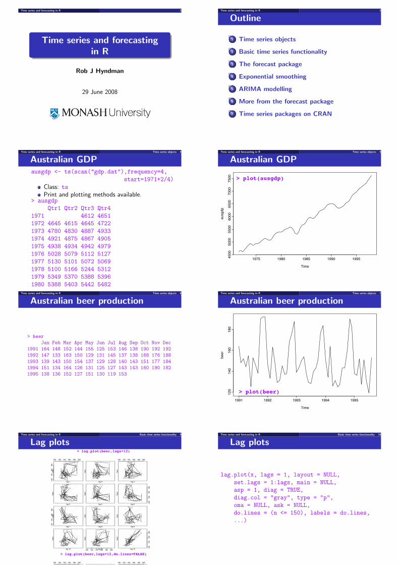
Time series and forecastingin R
Rob J Hyndman
29 June 2008
Time series and forecasting in R 2
Outline
1 Time series objects
2 Basic time series functionality
3 The forecast package
4 Exponential smoothing
5 ARIMA modelling
6 More from the forecast package
7 Time series packages on CRAN
Time series and forecasting in R Time series objects 4
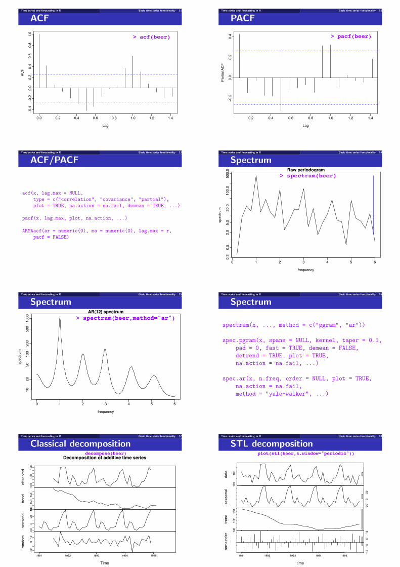
Australian GDPausgdp <- ts(scan("gdp.dat"),frequency=4,
start=1971+2/4)Class: tsPrint and plotting methods available.
> ausgdpQtr1 Qtr2 Qtr3 Qtr4
1971 4612 46511972 4645 4615 4645 47221973 4780 4830 4887 49331974 4921 4875 4867 49051975 4938 4934 4942 49791976 5028 5079 5112 51271977 5130 5101 5072 50691978 5100 5166 5244 53121979 5349 5370 5388 53961980 5388 5403 5442 5482
Time series and forecasting in R Time series objects 5
Australian GDP
Time
ausgdp
1975 1980 1985 1990 19954500
5000
5500
6000
6500
7000
7500
> plot(ausgdp)
Time series and forecasting in R Time series objects 6
Australian beer production
> beerJan Feb Mar Apr May Jun Jul Aug Sep Oct Nov Dec
1991 164 148 152 144 155 125 153 146 138 190 192 1921992 147 133 163 150 129 131 145 137 138 168 176 1881993 139 143 150 154 137 129 128 140 143 151 177 1841994 151 134 164 126 131 125 127 143 143 160 190 1821995 138 136 152 127 151 130 119 153
Time series and forecasting in R Time series objects 7
Australian beer production
Time
beer
1991 1992 1993 1994 1995
120
140
160
180
> plot(beer)
Time series and forecasting in R Basic time series functionality 9
Lag plots
lag 1
be
er 1
23
4
5
6
7
8
9
101112
13
14
15
16
1718
19
20 21
22
23
24
2526
2728
29
30 31
3233
34
35
36
37
38
39
40
41
4243
44 45
46
47
48
4950
51
52
53
54
55
12
01
40
16
01
80
100 120 140 160 180 200
lag 2
be
er 1
23
4
5
6
7
8
9
101112
13
14
15
16
1718
19
20 21
22
23
24
2526
2728
29
3031
3233
34
35
36
37
38
39
40
41
4243
44 45
46
47
48
4950
51
52
53
54
lag 3
be
er 1
23
4
5
6
7
8
9
1011 12
13
14
15
16
1718
19
20 21
22
23
24
2526
2728
29
30 31
3233
34
35
36
37
38
39
40
41
4243
4445
46
47
48
4950
51
52
53
100 120 140 160 180 200
lag 4
be
er 1
23
4
5
6
7
8
9
101112
13
14
15
16
1718
19
2021
22
23
24
2526
2728
29
30 31
3233
34
35
36
37
38
39
40
41
4243
4445
46
47
48
4950
51
52
lag 5
be
er 1
23
4
5
6
7
8
9
101112
13
14
15
16
1718
19
2021
22
23
24
2526
2728
29
30 31
3233
34
35
36
37
38
39
40
41
4243
4445
46
47
48
4950
51
lag 6
be
er 1
23
4
5
6
7
8
9
101112
13
14
15
16
1718
19
20 21
22
23
24
2526
2728
29
3031
3233
34
35
36
37
38
39
40
41
4243
44 45
46
47
48
4950
12
01
40
16
01
80
lag 7
be
er 1
23
4
5
6
7
8
9
1011 12
13
14
15
16
1718
19
2021
22
23
24
2526
2728
29
3031
3233
34
35
36
37
38
39
40
41
4243
4445
46
47
48
49
12
01
40
16
01
80
lag 8
be
er 1
23
4
5
6
7
8
9
101112
13
14
15
16
1718
19
2021
22
23
24
2526
2728
29
30 31
3233
34
35
36
37
38
39
40
41
4243
44 45
46
47
48
lag 9
be
er 1
23
4
5
6
7
8
9
101112
13
14
15
16
1718
19
2021
22
23
24
2526
2728
29
3031
3233
34
35
36
37
38
39
40
41
4243
4445
46
47
lag 10
be
er 1
23
4
5
6
7
8
9
1011 12
13
14
15
16
1718
19
2021
22
23
24
2526
2728
29
3031
3233
34
35
36
37
38
39
40
41
4243
4445
46
lag 11
be
er 1
23
4
5
6
7
8
9
1011 12
13
14
15
16
1718
19
20 21
22
23
24
2526
2728
29
3031
3233
34
35
36
37
38
39
40
41
4243
44 45
100 120 140 160 180 200lag 12
be
er 1
23
4
5
6
7
8
9
1011 12
13
14
15
16
1718
19
2021
22
23
24
2526
2728
29
3031
3233
34
35
36
37
38
39
40
41
4243
44
12
01
40
16
01
80
> lag.plot(beer,lags=12)
!
!!
!
!
!
!
!
!
!!!
!
!
!
!
!!
!
! !
!
!
!
!!
!!
!
! !
!!
!
!
!
!
!
!
!
!
!!
! !
!
!
!
!!
!
!
!
!
!
lag 1
be
er
12
01
40
16
01
80
100 120 140 160 180 200
!
!!
!
!
!
!
!
!
!!!
!
!
!
!
!!
!
! !
!
!
!
!!
!!
!
!!
!!
!
!
!
!
!
!
!
!
!!
! !
!
!
!
!!
!
!
!
!
lag 2
be
er !
!!
!
!
!
!
!
!
!! !
!
!
!
!
!!
!
! !
!
!
!
!!
!!
!
! !
!!
!
!
!
!
!
!
!
!
!!
!!
!
!
!
!!
!
!
!
lag 3
be
er
100 120 140 160 180 200
!
!!
!
!
!
!
!
!
!!!
!
!
!
!
!!
!
!!
!
!
!
!!
!!
!
! !
!!
!
!
!
!
!
!
!
!
!!
!!
!
!
!
!!
!
!
lag 4
be
er !
!!
!
!
!
!
!
!
!!!
!
!
!
!
!!
!
!!
!
!
!
!!
!!
!
! !
!!
!
!
!
!
!
!
!
!
!!
!!
!
!
!
!!
!
lag 5
be
er !
!!
!
!
!
!
!
!
!!!
!
!
!
!
!!
!
! !
!
!
!
!!
!!
!
!!
!!
!
!
!
!
!
!
!
!
!!
! !
!
!
!
!!
lag 6
be
er
12
01
40
16
01
80
!
!!
!
!
!
!
!
!
!! !
!
!
!
!
!!
!
!!
!
!
!
!!
!!
!
!!
!!
!
!
!
!
!
!
!
!
!!
!!
!
!
!
!
lag 7
be
er
12
01
40
16
01
80
!
!!
!
!
!
!
!
!
!!!
!
!
!
!
!!
!
!!
!
!
!
!!
!!
!
! !
!!
!
!
!
!
!
!
!
!
!!
! !
!
!
!
lag 8
be
er !
!!
!
!
!
!
!
!
!!!
!
!
!
!
!!
!
!!
!
!
!
!!
!!
!
!!
!!
!
!
!
!
!
!
!
!
!!
!!
!
!
lag 9
be
er
!
!!
!
!
!
!
!
!
!! !
!
!
!
!
!!
!
!!
!
!
!
!!
!!
!
! !
!!
!
!
!
!
!
!
!
!
!!
!!
!
lag 10
be
er !
!!
!
!
!
!
!
!
!! !
!
!
!
!
!!
!
! !
!
!
!
!!
!!
!
!!
!!
!
!
!
!
!
!
!
!
!!
! !
lag 11
be
er
100 120 140 160 180 200
!
!!
!
!
!
!
!
!
!! !
!
!
!
!
!!
!
!!
!
!
!
!!
!!
!
!!
!!
!
!
!
!
!
!
!
!
!!
!
lag 12
be
er
12
01
40
16
01
80
> lag.plot(beer,lags=12,do.lines=FALSE)
Time series and forecasting in R Basic time series functionality 10
Lag plots
lag.plot(x, lags = 1, layout = NULL,set.lags = 1:lags, main = NULL,asp = 1, diag = TRUE,diag.col = "gray", type = "p",oma = NULL, ask = NULL,do.lines = (n <= 150), labels = do.lines,...)
Time series and forecasting in R Basic time series functionality 11
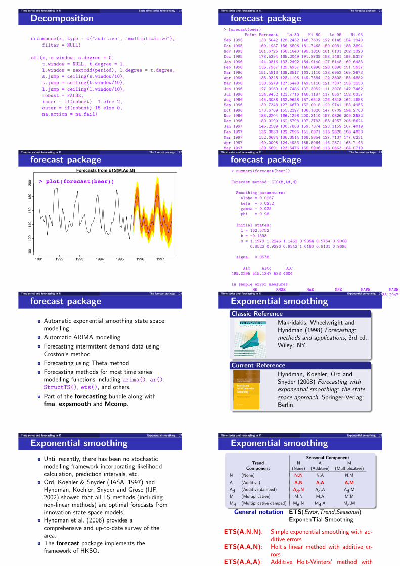
ACF
0.0 0.2 0.4 0.6 0.8 1.0 1.2 1.4
!0.4
!0.2
0.0
0.2
0.4
0.6
0.8
1.0
Lag
ACF
> acf(beer)
Time series and forecasting in R Basic time series functionality 12
PACF
0.2 0.4 0.6 0.8 1.0 1.2 1.4
!0.2
0.0
0.2
0.4
Lag
Part
ial A
CF
> pacf(beer)
Time series and forecasting in R Basic time series functionality 13
ACF/PACF
acf(x, lag.max = NULL,type = c("correlation", "covariance", "partial"),plot = TRUE, na.action = na.fail, demean = TRUE, ...)
pacf(x, lag.max, plot, na.action, ...)
ARMAacf(ar = numeric(0), ma = numeric(0), lag.max = r,pacf = FALSE)
Time series and forecasting in R Basic time series functionality 14
Spectrum
0 1 2 3 4 5 6
0.2
0.5
2.0
5.0
20.0
100.0
500.0
frequency
spectrum
Raw periodogram
> spectrum(beer)
Time series and forecasting in R Basic time series functionality 15
Spectrum
0 1 2 3 4 5 6
10
20
50
100
200
500
1000
frequency
spectrum
AR(12) spectrum
> spectrum(beer,method="ar")
Time series and forecasting in R Basic time series functionality 16
Spectrum
spectrum(x, ..., method = c("pgram", "ar"))
spec.pgram(x, spans = NULL, kernel, taper = 0.1,pad = 0, fast = TRUE, demean = FALSE,detrend = TRUE, plot = TRUE,na.action = na.fail, ...)
spec.ar(x, n.freq, order = NULL, plot = TRUE,na.action = na.fail,method = "yule-walker", ...)
Time series and forecasting in R Basic time series functionality 17
Classical decomposition
130
160
190
observed
146
150
154
trend
!20
020
40
seasonal
!20
010
1991 1992 1993 1994 1995
random
Time
Decomposition of additive time seriesdecompose(beer)
Time series and forecasting in R Basic time series functionality 18
STL decomposition
120
160
data
!20
020
seasonal
146
152
158
trend
!15
!5
515
1991 1992 1993 1994 1995
remainder
time
plot(stl(beer,s.window="periodic"))
Time series and forecasting in R Basic time series functionality 19
Decomposition
decompose(x, type = c("additive", "multiplicative"),filter = NULL)
stl(x, s.window, s.degree = 0,t.window = NULL, t.degree = 1,l.window = nextodd(period), l.degree = t.degree,s.jump = ceiling(s.window/10),t.jump = ceiling(t.window/10),l.jump = ceiling(l.window/10),robust = FALSE,inner = if(robust) 1 else 2,outer = if(robust) 15 else 0,na.action = na.fail)
Time series and forecasting in R The forecast package 21
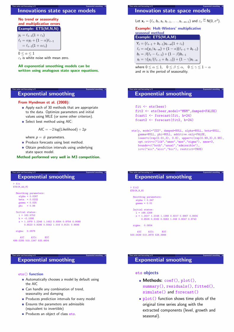
forecast package> forecast(beer)
Point Forecast Lo 80 Hi 80 Lo 95 Hi 95Sep 1995 138.5042 128.2452 148.7632 122.8145 154.1940Oct 1995 169.1987 156.6506 181.7468 150.0081 188.3894Nov 1995 181.6725 168.1640 195.1810 161.0131 202.3320Dec 1995 178.5394 165.2049 191.8738 158.1461 198.9327Jan 1996 144.0816 133.2492 154.9140 127.5148 160.6483Feb 1996 135.7967 125.4937 146.0996 120.0396 151.5537Mar 1996 151.4813 139.8517 163.1110 133.6953 169.2673Apr 1996 138.9345 128.1106 149.7584 122.3808 155.4882May 1996 138.5279 127.5448 149.5110 121.7307 155.3250Jun 1996 127.0269 116.7486 137.3052 111.3076 142.7462Jul 1996 134.9452 123.7716 146.1187 117.8567 152.0337Aug 1996 145.3088 132.9658 157.6518 126.4318 164.1858Sep 1996 139.7348 127.4679 152.0018 120.9741 158.4955Oct 1996 170.6709 155.2397 186.1020 147.0709 194.2708Nov 1996 183.2204 166.1298 200.3110 157.0826 209.3582Dec 1996 180.0290 162.6798 197.3783 153.4957 206.5624Jan 1997 145.2589 130.7803 159.7374 123.1159 167.4019Feb 1997 136.8833 122.7595 151.0071 115.2828 158.4838Mar 1997 152.6684 136.3514 168.9854 127.7137 177.6231Apr 1997 140.0008 124.4953 155.5064 116.2871 163.7145May 1997 139.5691 123.5476 155.5906 115.0663 164.0719Jun 1997 127.9620 112.7364 143.1876 104.6764 151.2476Jul 1997 135.9181 119.1567 152.6795 110.2837 161.5525Aug 1997 146.3349 127.6354 165.0344 117.7365 174.9332
Time series and forecasting in R The forecast package 22
forecast packageForecasts from ETS(M,Ad,M)
1991 1992 1993 1994 1995 1996 1997
100
120
140
160
180
200 > plot(forecast(beer))
Time series and forecasting in R The forecast package 23
forecast package> summary(forecast(beer))
Forecast method: ETS(M,Ad,M)
Smoothing parameters:alpha = 0.0267beta = 0.0232gamma = 0.025phi = 0.98
Initial states:l = 162.5752b = -0.1598s = 1.1979 1.2246 1.1452 0.9354 0.9754 0.9068
0.8523 0.9296 0.9342 1.0160 0.9131 0.9696
sigma: 0.0578
AIC AICc BIC499.0295 515.1347 533.4604
In-sample error measures:ME RMSE MAE MPE MAPE MASE
0.07741197 8.41555052 7.03312900 -0.29149125 4.78826138 0.43512047Time series and forecasting in R The forecast package 24
forecast package
Automatic exponential smoothing state spacemodelling.
Automatic ARIMA modelling
Forecasting intermittent demand data usingCroston’s method
Forecasting using Theta method
Forecasting methods for most time seriesmodelling functions including arima(), ar(),StructTS(), ets(), and others.
Part of the forecasting bundle along withfma, expsmooth and Mcomp.
Time series and forecasting in R Exponential smoothing 26
Exponential smoothingClassic Reference
Makridakis, Wheelwright andHyndman (1998) Forecasting:methods and applications, 3rd ed.,Wiley: NY.
Current ReferenceSpringer Series in Statistics
Rob J. Hyndman · Anne B. Koehler J. Keith Ord · Ralph D. Snyder
Forecasting with Exponential Smoothing
The State Space Approach
Forecasting with Exponential Sm
oothingHyndm
an · Koehler · Ord · Snyder
Hyndman, Koehler, Ord andSnyder (2008) Forecasting withexponential smoothing: the statespace approach, Springer-Verlag:Berlin.
Time series and forecasting in R Exponential smoothing 27
Exponential smoothing
Until recently, there has been no stochasticmodelling framework incorporating likelihoodcalculation, prediction intervals, etc.Ord, Koehler & Snyder (JASA, 1997) andHyndman, Koehler, Snyder and Grose (IJF,2002) showed that all ES methods (includingnon-linear methods) are optimal forecasts frominnovation state space models.Hyndman et al. (2008) provides acomprehensive and up-to-date survey of thearea.The forecast package implements theframework of HKSO.
Time series and forecasting in R Exponential smoothing 28
Exponential smoothing
Seasonal ComponentTrend N A M
Component (None) (Additive) (Multiplicative)
N (None) N,N N,A N,M
A (Additive) A,N A,A A,M
Ad (Additive damped) Ad,N Ad,A Ad,M
M (Multiplicative) M,N M,A M,M
Md (Multiplicative damped) Md,N Md,A Md,M
General notation ETS(Error,Trend,Seasonal)ExponenTial Smoothing
ETS(A,N,N): Simple exponential smoothing with ad-ditive errors
ETS(A,A,N): Holt’s linear method with additive er-rors
ETS(A,A,A): Additive Holt-Winters’ method withadditive errors
ETS(M,A,M): Multiplicative Holt-Winters’ methodwith multiplicative errors
ETS(A,Ad,N): Damped trend method with additive er-rors
There are 30 separate models in the ETSframework
Time series and forecasting in R Exponential smoothing 29
Innovations state space models
No trend or seasonalityand multiplicative errorsExample: ETS(M,N,N)
yt = !t!1(1 + "t)
!t = #yt + (1! #)!t!1
= !t!1(1 + #"t)
0 " # " 1"t is white noise with mean zero.
All exponential smoothing models can bewritten using analogous state space equations.
Time series and forecasting in R Exponential smoothing 30
Innovation state space models
Let xt = (!t , bt , st , st!1, . . . , st!m+1) and "tiid# N(0, $2).
Example: Holt-Winters’ multiplicativeseasonal methodExample: ETS(M,A,M)
Yt = (!t!1 + bt!1)st!m(1 + "t)
!t = #(yt/st!m) + (1! #)(!t!1 + bt!1)
bt = %(!t ! !t!1) + (1! %)bt!1
st = &(yt/(!t!1 + bt!1)) + (1! &)st!m
where 0 " # " 1, 0 " % " #, 0 " & " 1! #and m is the period of seasonality.
Time series and forecasting in R Exponential smoothing 31
Exponential smoothing
From Hyndman et al. (2008):Apply each of 30 methods that are appropriateto the data. Optimize parameters and initialvalues using MLE (or some other criterion).
Select best method using AIC:
AIC = !2 log(Likelihood) + 2p
where p = # parameters.
Produce forecasts using best method.
Obtain prediction intervals using underlyingstate space model.
Method performed very well in M3 competition.
Time series and forecasting in R Exponential smoothing 32
Exponential smoothing
fit <- ets(beer)fit2 <- ets(beer,model="MNM",damped=FALSE)fcast1 <- forecast(fit, h=24)fcast2 <- forecast(fit2, h=24)
ets(y, model="ZZZ", damped=NULL, alpha=NULL, beta=NULL,gamma=NULL, phi=NULL, additive.only=FALSE,lower=c(rep(0.01,3), 0.8), upper=c(rep(0.99,3),0.98),opt.crit=c("lik","amse","mse","sigma"), nmse=3,bounds=c("both","usual","admissible"),ic=c("aic","aicc","bic"), restrict=TRUE)
Time series and forecasting in R Exponential smoothing 33
Exponential smoothing> fitETS(M,Ad,M)
Smoothing parameters:alpha = 0.0267beta = 0.0232gamma = 0.025phi = 0.98
Initial states:l = 162.5752b = -0.1598s = 1.1979 1.2246 1.1452 0.9354 0.9754 0.9068
0.8523 0.9296 0.9342 1.016 0.9131 0.9696
sigma: 0.0578
AIC AICc BIC499.0295 515.1347 533.4604
Time series and forecasting in R Exponential smoothing 34
Exponential smoothing
> fit2ETS(M,N,M)
Smoothing parameters:alpha = 0.247gamma = 0.01
Initial states:l = 168.1208s = 1.2417 1.2148 1.1388 0.9217 0.9667 0.8934
0.8506 0.9182 0.9262 1.049 0.9047 0.9743
sigma: 0.0604
AIC AICc BIC500.0439 510.2878 528.3988
Time series and forecasting in R Exponential smoothing 35
Exponential smoothing
ets() function
Automatically chooses a model by default usingthe AIC
Can handle any combination of trend,seasonality and damping
Produces prediction intervals for every model
Ensures the parameters are admissible(equivalent to invertible)
Produces an object of class ets.
Time series and forecasting in R Exponential smoothing 36
Exponential smoothing
ets objects
Methods: coef(), plot(),summary(), residuals(), fitted(),simulate() and forecast()
plot() function shows time plots of theoriginal time series along with theextracted components (level, growth andseasonal).
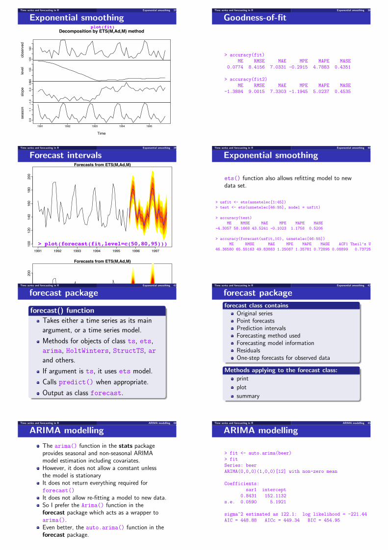
Time series and forecasting in R Exponential smoothing 37
Exponential smoothing120
160
observed
145
155
level
!1.0
0.0
0.5
slope
0.9
1.1
1991 1992 1993 1994 1995
season
Time
Decomposition by ETS(M,Ad,M) methodplot(fit)
Time series and forecasting in R Exponential smoothing 38
Goodness-of-fit
> accuracy(fit)ME RMSE MAE MPE MAPE MASE
0.0774 8.4156 7.0331 -0.2915 4.7883 0.4351
> accuracy(fit2)ME RMSE MAE MPE MAPE MASE
-1.3884 9.0015 7.3303 -1.1945 5.0237 0.4535
Time series and forecasting in R Exponential smoothing 39
Forecast intervalsForecasts from ETS(M,Ad,M)
1991 1992 1993 1994 1995 1996 1997
100
120
140
160
180
200
> plot(forecast(fit,level=c(50,80,95)))
Forecasts from ETS(M,Ad,M)
1991 1992 1993 1994 1995 1996 1997
100
120
140
160
180
200
> plot(forecast(fit,fan=TRUE))
Time series and forecasting in R Exponential smoothing 40
Exponential smoothing
ets() function also allows refitting model to newdata set.
> usfit <- ets(usnetelec[1:45])> test <- ets(usnetelec[46:55], model = usfit)
> accuracy(test)ME RMSE MAE MPE MAPE MASE
-4.3057 58.1668 43.5241 -0.1023 1.1758 0.5206
> accuracy(forecast(usfit,10), usnetelec[46:55])ME RMSE MAE MPE MAPE MASE ACF1 Theil’s U
46.36580 65.55163 49.83883 1.25087 1.35781 0.72895 0.08899 0.73725
Time series and forecasting in R Exponential smoothing 41
forecast package
forecast() functionTakes either a time series as its mainargument, or a time series model.
Methods for objects of class ts, ets,arima, HoltWinters, StructTS, arand others.
If argument is ts, it uses ets model.
Calls predict() when appropriate.
Output as class forecast.
Time series and forecasting in R Exponential smoothing 42
forecast packageforecast class contains
Original seriesPoint forecastsPrediction intervalsForecasting method usedForecasting model informationResidualsOne-step forecasts for observed data
Methods applying to the forecast class:print
plot
summary
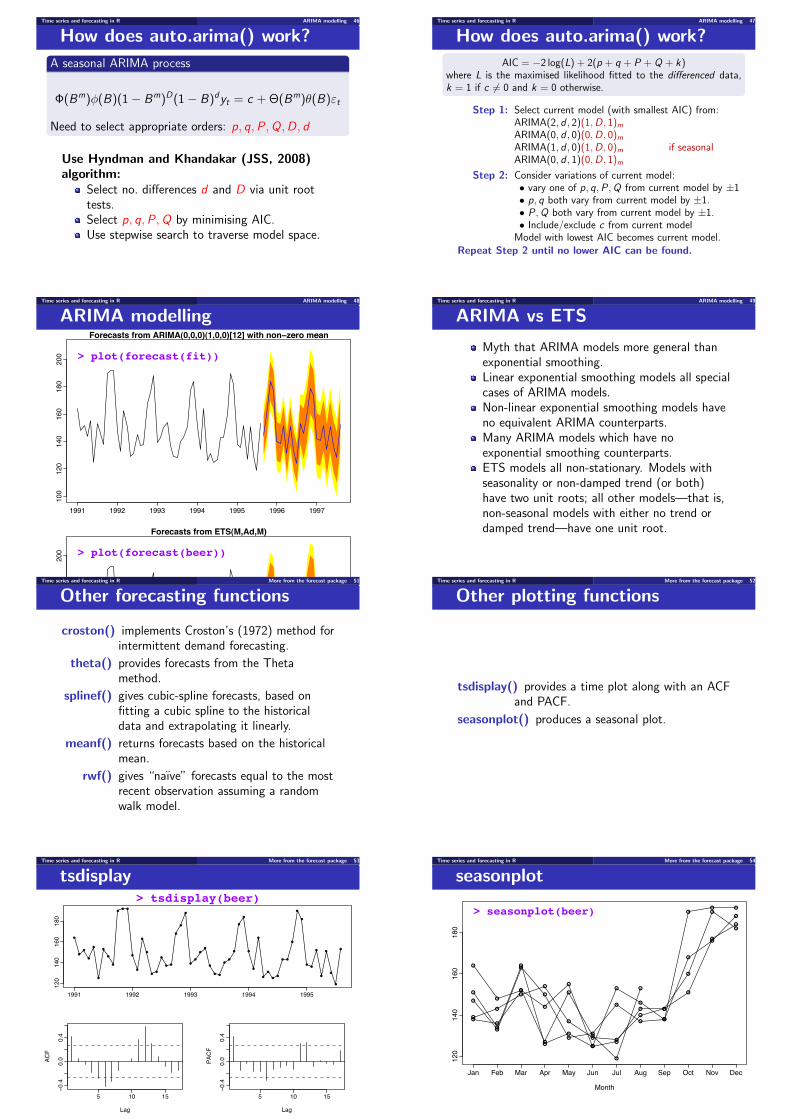
Time series and forecasting in R ARIMA modelling 44
ARIMA modelling
The arima() function in the stats packageprovides seasonal and non-seasonal ARIMAmodel estimation including covariates.However, it does not allow a constant unlessthe model is stationaryIt does not return everything required forforecast()It does not allow re-fitting a model to new data.So I prefer the Arima() function in theforecast package which acts as a wrapper toarima().Even better, the auto.arima() function in theforecast package.
Time series and forecasting in R ARIMA modelling 45
ARIMA modelling
> fit <- auto.arima(beer)> fitSeries: beerARIMA(0,0,0)(1,0,0)[12] with non-zero mean
Coefficients:sar1 intercept
0.8431 152.1132s.e. 0.0590 5.1921
sigma^2 estimated as 122.1: log likelihood = -221.44AIC = 448.88 AICc = 449.34 BIC = 454.95
Time series and forecasting in R ARIMA modelling 46
How does auto.arima() work?
A seasonal ARIMA process
!(Bm)'(B)(1! Bm)D(1! B)dyt = c + "(Bm)((B)"t
Need to select appropriate orders: p, q, P , Q, D, d
Use Hyndman and Khandakar (JSS, 2008)algorithm:
Select no. di#erences d and D via unit roottests.Select p, q, P , Q by minimising AIC.Use stepwise search to traverse model space.
Time series and forecasting in R ARIMA modelling 47
How does auto.arima() work?AIC = !2 log(L) + 2(p + q + P + Q + k)
where L is the maximised likelihood fitted to the di!erenced data,k = 1 if c $= 0 and k = 0 otherwise.
Step 1: Select current model (with smallest AIC) from:ARIMA(2, d , 2)(1, D, 1)m
ARIMA(0, d , 0)(0, D, 0)m
ARIMA(1, d , 0)(1, D, 0)m if seasonalARIMA(0, d , 1)(0, D, 1)m
Step 2: Consider variations of current model:• vary one of p, q, P , Q from current model by ±1• p, q both vary from current model by ±1.• P , Q both vary from current model by ±1.• Include/exclude c from current model
Model with lowest AIC becomes current model.Repeat Step 2 until no lower AIC can be found.
Time series and forecasting in R ARIMA modelling 48
ARIMA modellingForecasts from ARIMA(0,0,0)(1,0,0)[12] with non!zero mean
1991 1992 1993 1994 1995 1996 1997
100
120
140
160
180
200 > plot(forecast(fit))
Forecasts from ETS(M,Ad,M)
1991 1992 1993 1994 1995 1996 1997
100
120
140
160
180
200 > plot(forecast(beer))
Time series and forecasting in R ARIMA modelling 49
ARIMA vs ETS
Myth that ARIMA models more general thanexponential smoothing.Linear exponential smoothing models all specialcases of ARIMA models.Non-linear exponential smoothing models haveno equivalent ARIMA counterparts.Many ARIMA models which have noexponential smoothing counterparts.ETS models all non-stationary. Models withseasonality or non-damped trend (or both)have two unit roots; all other models—that is,non-seasonal models with either no trend ordamped trend—have one unit root.
Time series and forecasting in R More from the forecast package 51
Other forecasting functions
croston() implements Croston’s (1972) method forintermittent demand forecasting.
theta() provides forecasts from the Thetamethod.
splinef() gives cubic-spline forecasts, based onfitting a cubic spline to the historicaldata and extrapolating it linearly.
meanf() returns forecasts based on the historicalmean.
rwf() gives “naıve” forecasts equal to the mostrecent observation assuming a randomwalk model.
Time series and forecasting in R More from the forecast package 52
Other plotting functions
tsdisplay() provides a time plot along with an ACFand PACF.
seasonplot() produces a seasonal plot.
Time series and forecasting in R More from the forecast package 53
tsdisplay
1991 1992 1993 1994 1995
120
140
160
180
!
!
!
!
!
!
!
!
!
!! !
!
!
!
!
!!
!
!!
!
!
!
!
!
!
!
!
!!
!
!
!
!
!
!
!
!
!
!
!!
! !
!
!
!
!!
!
!
!
!
!
!
5 10 15
!0.4
0.0
0.4
Lag
ACF
5 10 15
!0.4
0.0
0.4
Lag
PACF
> tsdisplay(beer)
Time series and forecasting in R More from the forecast package 54
seasonplot
!
!
!
!
!
!
!
!
!
!! !
!
!
!
!
!!
!
!!
!
!
!
!
!
!
!
!
!!
!
!
!
!
!
!
!
!
!
!
!!
! !
!
!
!
!!
!
!
!
!
!
!
120
140
160
180
Month
Jan Feb Mar Apr May Jun Jul Aug Sep Oct Nov Dec
> seasonplot(beer)

Time series and forecasting in R Time series packages on CRAN 56
Basic facilities
stats Contains substantial time seriescapabilities including the ts class forregularly spaced time series. Also ARIMAmodelling, structural models, time seriesplots, acf and pacf graphs, classicaldecomposition and STL decomposition.
Time series and forecasting in R Time series packages on CRAN 57
Forecasting and univariatemodelling
forecast Lots of univariate time series methodsincluding automatic ARIMA modelling,exponential smoothing via state spacemodels, and the forecast class forconsistent handling of time seriesforecasts. Part of the forecastingbundle.
tseries GARCH models and unit root tests.FitAR Subset AR model fitting
partsm Periodic autoregressive time series modelspear Periodic autoregressive time series models
Time series and forecasting in R Time series packages on CRAN 58
Forecasting and univariatemodelling
ltsa Methods for linear time series analysisdlm Bayesian analysis of Dynamic Linear Models.
timsac Time series analysis and controlfArma ARMA ModellingfGarch ARCH/GARCH modelling
BootPR Bias-corrected forecasting and bootstrapprediction intervals for autoregressivetime series
gsarima Generalized SARIMA time series simulationbayesGARCH Bayesian Estimation of the
GARCH(1,1) Model with t innovations
Time series and forecasting in R Time series packages on CRAN 59
Resampling and simulation
boot Bootstrapping, including the blockbootstrap with several variants.
meboot Maximum Entropy Bootstrap for TimeSeries
Time series and forecasting in R Time series packages on CRAN 60
Decomposition and filtering
robfilter Robust time series filtersmFilter Miscellaneous time series filters useful for
smoothing and extracting trend andcyclical components.
ArDec Autoregressive decompositionwmtsa Wavelet methods for time series analysis
based on Percival and Walden (2000)wavelets Computing wavelet filters, wavelet
transforms and multiresolution analysessignalextraction Real-time signal extraction
(direct filter approach)bspec Bayesian inference on the discrete power
spectrum of time series
Time series and forecasting in R Time series packages on CRAN 61
Unit roots and cointegration
tseries Unit root tests and methods forcomputational finance.
urca Unit root and cointegration tests
uroot Unit root tests including methods forseasonal time series
Time series and forecasting in R Time series packages on CRAN 62
Nonlinear time series analysis
nlts R functions for (non)linear timeseries analysis
tseriesChaos Nonlinear time series analysisRTisean Algorithms for time series analysis
from nonlinear dynamical systemstheory.
tsDyn Time series analysis based ondynamical systems theory
BAYSTAR Bayesian analysis of thresholdautoregressive models
fNonlinear Nonlinear and Chaotic Time SeriesModelling
bentcableAR Bent-Cable autoregression
Time series and forecasting in R Time series packages on CRAN 63
Dynamic regression models
dynlm Dynamic linear models and time seriesregression
dyn Time series regression
tpr Regression models with time-varyingcoe$cients.
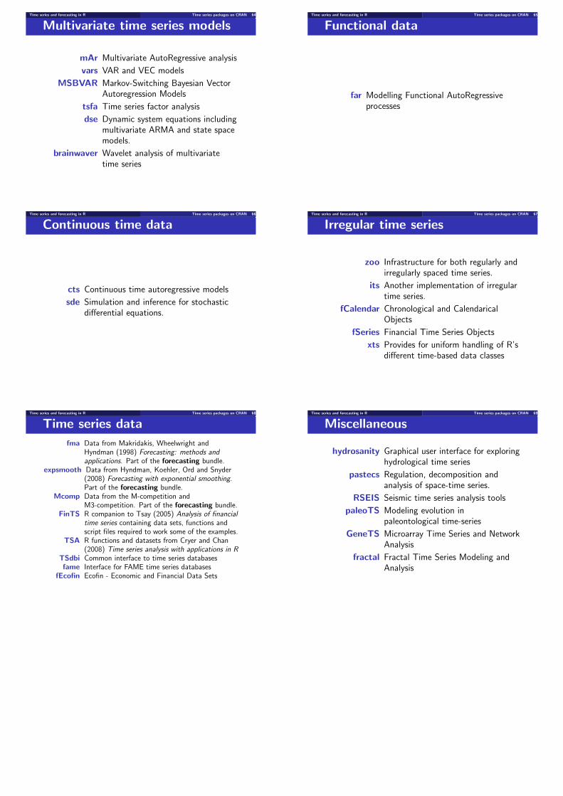
Time series and forecasting in R Time series packages on CRAN 64
Multivariate time series models
mAr Multivariate AutoRegressive analysis
vars VAR and VEC models
MSBVAR Markov-Switching Bayesian VectorAutoregression Models
tsfa Time series factor analysis
dse Dynamic system equations includingmultivariate ARMA and state spacemodels.
brainwaver Wavelet analysis of multivariatetime series
Time series and forecasting in R Time series packages on CRAN 65
Functional data
far Modelling Functional AutoRegressiveprocesses
Time series and forecasting in R Time series packages on CRAN 66
Continuous time data
cts Continuous time autoregressive models
sde Simulation and inference for stochasticdi#erential equations.
Time series and forecasting in R Time series packages on CRAN 67
Irregular time series
zoo Infrastructure for both regularly andirregularly spaced time series.
its Another implementation of irregulartime series.
fCalendar Chronological and CalendaricalObjects
fSeries Financial Time Series Objects
xts Provides for uniform handling of R’sdi#erent time-based data classes
Time series and forecasting in R Time series packages on CRAN 68
Time series datafma Data from Makridakis, Wheelwright and
Hyndman (1998) Forecasting: methods andapplications. Part of the forecasting bundle.
expsmooth Data from Hyndman, Koehler, Ord and Snyder(2008) Forecasting with exponential smoothing.Part of the forecasting bundle.
Mcomp Data from the M-competition andM3-competition. Part of the forecasting bundle.
FinTS R companion to Tsay (2005) Analysis of financialtime series containing data sets, functions andscript files required to work some of the examples.
TSA R functions and datasets from Cryer and Chan(2008) Time series analysis with applications in R
TSdbi Common interface to time series databasesfame Interface for FAME time series databases
fEcofin Ecofin - Economic and Financial Data Sets
Time series and forecasting in R Time series packages on CRAN 69
Miscellaneous
hydrosanity Graphical user interface for exploringhydrological time series
pastecs Regulation, decomposition andanalysis of space-time series.
RSEIS Seismic time series analysis tools
paleoTS Modeling evolution inpaleontological time-series
GeneTS Microarray Time Series and NetworkAnalysis
fractal Fractal Time Series Modeling andAnalysis


