RSTUNE

RSTune™User’s Guide

September 2000

Contacting RockwellSoftware

Technical Support Telephone — 440-646-7800Technical Support Fax — 440-646-7801World Wide Web—www.software.rockwell.com

Copyright Notice ©2000 Rockwell Software Inc., a Rockwell Automation company All rights reservedPrinted in the United States of AmericaPortions copyrighted by ExperTune Inc. and used with permission. Portions copyrighted by Allen-Bradley Company, Inc., and used with permission.Inc. and John Gerry of ExperTune Inc. and used with permission.This manual and any accompanying Rockwell Software products are copyrighted by Rockwell Software Inc. Any reproduction and/or distribution without prior written consent from Rockwell Software Inc. is strictly prohibited. Please refer to the license agreement for details.

Trademark Notices WINtelligent Series is a registered trademark, and the Rockwell Software logo, RSAlarm, RSAnimator, RSAssistant, RSBatch, RSBreakerBox, RSButton, RSChart, RSCompare, RSControlRoom, RSData, RSDataPlayer, RSEventMaster, RSGauge, RSJunctionBox, RSLogix Emulate 5, RSLogix Emulate 500, RSGuardian, RSHarmony, RSKeys, RSLadder, RSLadder 5, RSLadder 500, RSLinx, RSLogix 5, RSLogix 500, RSLogix Frameworks, RSLogix SL5, RSMailman, RSNetworx for ControlNet, RSNetworx for DeviceNet, RSPortal, RSPower, RSPowerCFG, RSPowerRUN, RSPowerTools, RSRules, RSServer32, RSServer, RSServer OPC Toolkit, RSSidewinderX, RSSlider, RSSnapshot, RSSql, RSToolbox, RSToolPak I, RSToolPak II, RSTools, RSTrainer, RSTrend, RSTune, RSVessel, RSView32, RSView, RSVisualLogix, RSWheel, RSWire, RSWorkbench, RSWorkshop, SoftLogix 5, A.I. Series, Advanced Interface (A.I.) Series, AdvanceDDE, AutomationPak, ControlGuardian, ControlPak, ControlView, INTERCHANGE, Library Manager, Logic Wizard, Packed DDE, ProcessPak, ProcessPak5, ProcessPak for Batch, View Wizard, WINtelligent, WINtelligent LINX, WINtelligent LOGIC 5, WINtelligent VIEW, WINtelligent RECIPE, WINtelligent VISION, and WINtelligent VISION2 are trademarks of Rockwell Software Inc.PLC, PLC-2, PLC-3 and PLC-5 are registered trademarks, and Data Highway Plus, DH+, DHII, DTL, MicroLogix, Network DTL, PowerText, Pyramid Integrator, PanelBuilder, PanelView, ControlLogix, PLC-5/250, PLC-5/20E, PLC-5/40E, PLC-5/80E, ProcessLogix, SLC, SLC 5/01, SLC 5/02, SLC 5/03, SLC 5/04, SLC 5/05, SLC 500, and SoftLogix are trademarks of the Allen-Bradley Company, Inc.Microsoft, MS-DOS, Windows, Visual SourceSafe, and Visual Basic are registered trademarks, and Windows NT, Windows 95, Windows 98, and Microsoft Access are trademarks of the Microsoft Corporation.ControlNet is a trademark of ControlNet International.DeviceNet is a trademark of the Open DeviceNet Vendors Association.Ethernet is a registered trademark of Digital Equipment Corporation, Intel, and Xerox Corporation.Pentium is a registered trademark of the Intel Corporation.Adobe and Acrobat are trademarks of Adobe Systems Incorporated.IBM is a registered trademark of International Business Machines Corporation. AIX, PowerPC, Power Series, RISC System/6000 are trademarks of International Business Machines Corporation.UNIX is a registered trademark in the United States and other countries, licensed exclusively through X/Open Company Limited.AutoCAD is a registered trademark of Autodesk, Inc.All other trademarks are the property of their respective holders and are hereby acknowledged.

Warranty This Rockwell Software product is warranted in accord with the product license. The product’s performance will be affected by system configuration, the application being performed, operator control and other related factors.The product’s implementation may vary among users. This manual is as up-to-date as possible at the time of printing; however, the accompanying software may have changed since that time. Rockwell Software reserves the right to change any information contained in this manual or the software at any time without prior notice.The instructions in this manual do not claim to cover all the details or variations in the equipment, procedure, or process described, nor to provide directions for meeting every possible contingency during installation, operation, or maintenance.

Table of ContentsChapter 1Introduction .......................................................................................................................................... 1

What is RSTune™? ................................................................................................................. 1

RSTune Features..................................................................................................................... 1

System and software requirements .......................................................................... 2

Chapter 2Installation............................................................................................................................................. 5

Setting up RSLinx for RSTune ....................................................................................... 5

Installing RSTune.................................................................................................................... 7

Starting the RSTune software ....................................................................................... 8

Configuring a loop to communicate with a processor ................................. 8

Editing and deleting loops.............................................................................................. 11Editing an existing loop ................................................................................................................. 11Deleting a loop ................................................................................................................................ 12

Testing communications ................................................................................................. 12

Troubleshooting installation......................................................................................... 13

Chapter 3Quick Start ........................................................................................................................................... 15

Tuning a loop ........................................................................................................................... 15

Guidelines for optimizing loops .................................................................................. 16

Chapter 4Tuning theory .................................................................................................................................... 19

Description of proportional, integral, and derivative control ............... 19

� i

PID loop example .................................................................................................................. 21Proportional only control .............................................................................................................. 22Proportional plus integral (PI) control ........................................................................................ 23Proportional plus integral plus derivative (PID) control .......................................................... 23

RSTune theory ........................................................................................................................ 24Tuning types .................................................................................................................................... 24

Chapter 5Using RSTune ................................................................................................................................... 27

Faceplate and Trend window....................................................................................... 28

Changing the display of the Faceplate and Trend window .................... 29Changing the Trend display........................................................................................................... 29Changing the span, colors, and decimal places .......................................................................... 30Changing the value of the left and right axes ............................................................................. 31Changing the display of the Faceplate and Trend window ...................................................... 31

Using the Off Line Analysis & PID Tuning screen ......................................... 33

Changing controller settings........................................................................................ 34Changing the setpoint and controller output ............................................................................. 34Changing the controller mode ...................................................................................................... 34

Debugging communications ......................................................................................... 35

Menus ............................................................................................................................................ 35Faceplate and Trend window options menu .............................................................................. 36Faceplate buttons ............................................................................................................................ 36AutoTune ......................................................................................................................................... 38Close.................................................................................................................................................. 38Simulate window ............................................................................................................................. 38

Creating a report for a control loop......................................................................... 41About the report ............................................................................................................................. 41

Setting up extra trends .................................................................................................... 42

Chapter 6Tuning control loops ................................................................................................................ 45

Collecting data ....................................................................................................................... 45

Using AutoTune to collect data ................................................................................. 45

ii � RSTune User’s Guide

Manually collecting data ................................................................................................. 48Collecting data manually ................................................................................................................ 48Data pair and sample interval requirements ............................................................................... 49

Using archived data files ................................................................................................ 50Archiving data.................................................................................................................................. 50Using archived data......................................................................................................................... 50Tuning from archived data ............................................................................................................ 51Deleting archived files .................................................................................................................... 51Adding notes to an archived data file ..........................................................................................51Saving archived data to a different format .................................................................................. 52Changing and downloading PID parameters to the controller................................................ 55

Chapter 7Using the Time data window.......................................................................................... 57

Time Data Toolbar ......................................................................................................................... 58

Changing the Time data window display............................................................. 59Changing line weight ...................................................................................................................... 59Changing the graph type ................................................................................................................ 59

Calculating tuning parameters ................................................................................... 59

Controller tuning ................................................................................................................... 61

Editing data in the Time data window................................................................... 62Zooming ........................................................................................................................................... 62Averaging data ................................................................................................................................. 64Changing data points to a line....................................................................................................... 65Saving changes................................................................................................................................. 66

Verifying data using the Time data window...................................................... 66Statistical analysis ............................................................................................................................ 66Hysteresis check .............................................................................................................................. 68Notes on the hysteresis check....................................................................................................... 70

Adding data from the Time data window to the report ............................. 71

Chapter 8Control loop analysis ............................................................................................................... 73

Using the standard analysis tools ............................................................................ 73

Selecting a process model ............................................................................................ 74

� iii

Options in the Process Model window .................................................................. 76Model Type ...................................................................................................................................... 76Starting the Simulator..................................................................................................................... 76

Process Frequency Response (Bode) plot.......................................................... 77

Control Loop Simulation plot ....................................................................................... 78Options in the Control Loop Simulation plot............................................................................ 79Setpoint plot .................................................................................................................................... 79Load plot .......................................................................................................................................... 79

Robustness plot ..................................................................................................................... 80Options in the Robustness plot .................................................................................................... 81

Chapter 9Application notes ......................................................................................................................... 83

Data collection methods ................................................................................................. 83Controller in manual (open loop)................................................................................................. 84Controller in auto (closed loop).................................................................................................... 84Controller in auto (using a manual step test).............................................................................. 84Controller in manual (fast plant test) ........................................................................................... 85

Examples of data editing ................................................................................................ 86Example of noisy data.................................................................................................................... 86Example of data that is cycling and has noise spikes ................................................................ 86Example of a process that responds faster in one direction .................................................... 88

Integrating (non-self-regulating) loops.................................................................. 89

Temperature control of extruders ............................................................................ 89

Cascading loops .................................................................................................................... 90Collecting data for cascading loops.............................................................................................. 91

Chapter 10Getting the information you need ............................................................................. 93

Introduction .............................................................................................................................. 93

Supplemental reading ....................................................................................................... 93

Online help................................................................................................................................. 94

Online Books ............................................................................................................................ 94

iv � RSTune User’s Guide

Technical support services ........................................................................................... 94When you call .................................................................................................................................. 95

DDE topics ............................................................................................................................................ 97

What is a DDE topic? .......................................................................................................... 97Single processor example............................................................................................................... 98

Recommendations for programming PID loops ........................................ 99

Ladder logic considerations ......................................................................................... 99

Processor considerations .............................................................................................100PLC-5 processors ..........................................................................................................................100SLC 500 processors ......................................................................................................................100ControlLogix processors..............................................................................................................100

Loop setup parameters in RSTune .........................................................................101Control block address...................................................................................................................101Control variable address...............................................................................................................102Process variable address...............................................................................................................102PV or SP engineering units..........................................................................................................102

Activation ............................................................................................................................................103

How activation works......................................................................................................103

Protecting your activation files ................................................................................104

Activating RSTune .............................................................................................................105Running the activation utilities....................................................................................................105

Finding more information about activation......................................................106

Some common questions ..............................................................................................106Glossary ................................................................................................................................................109

� v

vi � RSTune User’s Guide

Chapter

IntroductionWelcome to RSTune, the application that makes tuning your control loops fast, easy, and accurate. RSTune also provides methods of analyzing your loops to help ensure optimal tuning parameters.This chapter covers:• What is RSTune™?• RSTune Features• System and software requirements

What is RSTune™?RSTune is Rockwell Software’s Windows®-based software for analyzing and tuning PID control loops in Allen-Bradley® PLC-5®, SLC 500™, and ControlLogix Programmable Logic Controllers.

RSTune Features• Toolbars on the time plot: makes zooming, editing, averaging, or filtering

your real-time data a snap• OPC support: RSTune is an OPC client (RSLinx 2.1 and above only).• ControlLogix 5550 support

• Support for MicroLogix 1200 and MicroLogix 1500

• Support for Logix 5000 PID function block

• Extra trend: An extra trend can be added to allow you to watch another variable in the same trend.

• Viewing of real-time trend values: Real-time trend values can be viewed as ToolTips by positioning the cursor on the trend line.

• View part of a Control Loop simulation: Easily expand or halve the range on the simulation plot. Lets you view the part of the simulation that interests you most.

Introduction � 1

• Seamless connectivity to your control loops: RSTune uses RSLinx™ Standard, Professional or OEM (OPC only) for all supported processors. The RSTune family of products does not work with RSLinx Lite.

• AutoTune: Easy-to-use AutoTune sequence reduces the time required to tune a loop from hours to minutes

• Archiving: Manual archiving of multiple sets of data allows easy before and after analysis

• Performance increase displays: The performance increase from tuning your loop is displayed on the Faceplate.

• PID loop tuning categories: Categories can be selected for load tuning or setpoint tuning from the simulation plot

• Pre-download setting analysis: Allows you to see the performance of your loops before actually downloading them to the controller

• Data optimization: Data can be zoomed, filtered, averaged, and line edited• Control loop testing: RSTune includes powerful analysis plots that

provide critical performance information on your loops.• Hysteresis check: Allows you to determine whether your control

elements (e.g. valves) are suffering from hysteresis• Tuning reports: Include data, notes, and graphics

System and software requirements• IBM®-compatible 486 or greater (Pentium™ recommended)• Microsoft® Windows® 95, Windows 98, Windows NT™ (4.0, Service Pack

3 or 4)• If reporting function will be used, Microsoft® Word 97 with SR-1 or higher• 8 MB of hard disk space (or more based on application requirements)• 16-color VGA graphics adapter 640 x 480 (256-color or higher, 800 x 600

recommended)• Any Windows®-compatible pointing device• Communications software

• Windows NT: RSLinx 1.50.58 (or higher) • Windows 95 / 98 / 2000 : RSLinx 1.50.58 (or higher)

2 � RSTune User’s Guide

.

Tip Lite or OEM versions of the communications software are not sufficient for communication with RSTune. You must have at least the standard version of the communications software.

Introduction � 3


Chapter

InstallationThis chapter provides information on installing RSTune and setting up the communications package.You must have communication software installed and configured for RSTune to communicate with your control loop. RSTune works with:� RSLinxYou can create a simulated control loop in RSTune without communication software.These topics are covered in this chapter:� Setting up RSLinx for RSTune� Installing RSTune� Starting the RSTune software� Configuring a loop to communicate with a processor� Editing and deleting loops� Testing communications� Troubleshooting installation

Setting up RSLinx for RSTuneTo have RSTune communicate to your processor, you must have RSLinx configured and running. For each processor that RSTune will communicate with, you need to have an RSLinx DDE/OPC Topic defined.

These steps are not needed if you are using the control loop simulator.To configure an RSTune loop to communicate with your processor:1. Install RSLinx.2. Configure RSLinx to communicate with your processor.

Tip This section provides an overview of the steps required in the communication software. For more information on configuring the software and defining a DDE/OPC topic, see Appendix A, “DDE topics” and the RSLinx documentation.

Installation � 5

3. Define an RSLinx topic that RSTune can use to communicate with your PLC.


Installing RSTuneYour RSTune package contains a CD-ROM and a Master Disk. RSTune is copy protected, and the Master Disk activates the software.To install the RSTune software on Windows 95, Windows 98, or Windows NT 4.0 operating systems:1. Close all open programs in Windows.2. Insert the RSTune CD-ROM into the drive.3. Click Start, then click Run. The Run dialog box is displayed.4. In the Open edit box, type drive:\setup, where drive is the letter of the

drive containing the CD-ROM. Click OK.5. Follow the directions on the screen.6. When prompted for the product’s serial number, enter the 10-digit serial

number on the label of the Master Disk.7. When asked if you want to move activation now, click Yes. Insert the

Master Disk into the disk drive.The utility for moving activation, EvMove, runs. Use the EvMove dialogs to move activation from the Master Disk to your root directory (usually C:). For help using EvMove, see Appendix C, “Activation,” or the EvMove online help.

8. Remove the Master Disk and follow the directions on the screen. When the setup utility finishes, an entry for the RSTune application program is displayed in the program list in the Rockwell Software group.

9. Store the CD-ROM and the Master Disk in a safe place.

Tip For more information on activation, see Appendix C, “Activation.”

Installation � 7

Starting the RSTune softwareTo start RSTune software on a PC:1. Click Start.2. Select Programs > Rockwell Software > RSTune.3. Select RSTune.

The main window is displayed.

From this window you can define a new loop, choose an existing loop to either tune or edit, or delete a loop. Loops that have already been created are listed in the Choose a Loop box in the main window. For more information, see “Editing and deleting loops” on page 11.

Configuring a loop to communicate with a processorIn RSTune, you must define parameters for each loop you want to tune.These steps are not needed if you are using the control loop simulator.

Tip Important information about programming the PID instruction in your processor is in Appendix B, “Recommendations for programming PID loops.”We recommend using the PD file type when you program the PID loop if you are using a New Platform PLC-5 processor.


1. Start RSTune.2. On the RSTune main window, click New Loop.

This window is displayed.

3. Type a name for the loop in the File name box. The file extension .tun is added automatically.

4. Click Save. The RSTune Setup window is displayed, as shown here.

5. Choose the Processor Type. The Setup window changes to show the options for the selected processor.

6. If the communications package provides both DDE and OPC support, the DDE and OPC options are available under Communications Via. Select the type of communication you want to use.

7. Complete the boxes as described in this table.

Installation � 9

If you selected this processor: Set these parameters: Parameter descriptions

PLC-5 PD filePLC-5 integer fileSLC 5/03, 5/04SLC 5/02, 5/05ControlLogixMicroLogix 1200/1500

PV Engineering units The engineering units displayed by the AutoTune sequence when it requests a setpoint change. These units are for display only.

Topic The RSLinx Topic. You can select the topic from the drop-down list.

(All processors) Sample Interval The sample interval of your controller or to an interval 4 to 10 times less than the equivalent dead time of your process. Equivalent dead time is the time it takes for your process variable to change appreciably after the controller output changes.RSTune uses the sample interval time to:� collect data to analyze� update the faceplate trend and bar graphs

PLC-5 PD filePLC-5 integer fileSLC 5/03, 5/04SLC 5/02, 5/05ControlLogixMicroLogix 1200/1500

Loop Update Time The Loop Update Time is a parameter that is held inside the PID control block. It needs to be set when you are programming the block. When the PID control block executes, it uses the Loop Update Time in the PID calculation. It is important that the Loop Update Time in the control block corresponds exactly to the actual sample period of the loop. The PID control block should be activated by a timer. The timer preset value should therefore be the same as the Loop Update Time. If this is not the case the PID calculation will be incorrect.The SLC PID instruction can operate in Timed mode or in STI mode. In Timed mode the instruction executes every Update Time period. In STI mode, the instruction should be placed in an STI interrupt subroutine. It will then execute every time the STI subroutine is scanned.

PLC-5 PD filePLC-5 integer fileSLC 5/03, 5/04SLC 5/02, 5/05

PID Instruction Addresses

The addresses used in the PID instruction in your ladder logic file. The Processor Type determines how many addresses are required.


8. Click Save.9. To:

� Return to the main window: Click Close.� Add trends or loops: See “Setting up extra trends” on page 42 .� Go to the Faceplate and Trend window: Click Faceplate.

Editing and deleting loops

Editing an existing loopThe setup parameters for an existing loop can be edited at any time.To edit an existing loop:1. Click the name of the loop in the Choose a Loop list.

2. Click Edit Setup. The RSTune Setup dialog box is displayed. See “Configuring a loop to communicate with a processor” on page 8 for detail on the options in this dialog box.

ControlLogix Tags scoped to program files

Tags in ControlLogix can be scoped to either controllers or program files. If your tags are scoped to program files, select the check box.If you select the check box, the Program file box is displayed. Type the name of the program where your PID control block loop tag resides. Type it in the same format as it was entered when you programmed the PID instruction.

Tag Name The tag name of the PID control block.

If you selected this processor: Set these parameters: Parameter descriptions

Installation � 11

Deleting a loopTo delete a loop (a .tun file and all associated data files):1. In the main window, click the loop to delete in the Choose a Loop list.2. Select File > Delete Loop.3. To:

� Delete archived data for this loop: Select Yes to question in the dialog box.

� Keep archived data for this loop: Select No to question in the dialog box. Data can be deleted manually later if desired.

Testing communicationsThe link between RSTune and the server can be either DDE or OPC. RSTune automatically determines the available communications methods. If there is a choice, you can choose between DDE or OPC in the Edit Setup window.You can test the communications through the Setup dialog box to see if the server is responding correctly.To test communications, click Test.RSTune attempts to read the process variable for the loop from the server. RSTune shows either an error message or the current process variable of the loop.

Tip When you are editing an existing control loop, options in the RSTune Setup dialog box are grayed out if there is archived data stored for that loop.Archives are created:� by RSTune when you run the AutoTune sequence� when you select Archive>Archive OnTo select a new PID loop or change the location, do one of the following:� Click Save As to create a new loop.� Click Close to go to the main window. Click New to create a new

loop.


Troubleshooting installationIf RSTune does not start up or run properly, check the following.

� Is the communication software installed? RSTune works with RSLinx version 1.50.58 or later. The communication software provides communication between the programmable controller and a personal computer in the Microsoft Windows NT, Windows 95, or Windows 98 environment.

If you get a LINX Initialization error message in RSTune when you try to call up the Control Loop Setup window, check these items.� Check the configuration of the RSLinx topic for proper station address and

communications device.� Make sure your cable or card is plugged in.� Check the RSLinx topic to be sure that the Station number is set to the node

address of the processor with which you want to communicate.� If you get the error “Foreign application won’t perform DDE method or

operation,” you might have tried to access the faceplate before all of the RSLinx drivers have fully initialized. Wait and then try again.

� Check to see if RSLinx is running. If not, did you install it? Can you run RSLinx by itself?

� Check to see if your Control Block address is pointing to a PID controller.

Installation � 13


Chapter

Quick StartThis chapter gives you a step-by-step approach to get you started using RSTune. More detailed explanations about the tuning process and how you can edit, verify, and analyze your data can be found in the remaining chapters of this User’s Guide.These topics are covered:� Tuning a loop� Guidelines for optimizing loops

Tuning a loop1. Click Faceplate to communicate with your PID loop or software

simulation. The Faceplate window is displayed.

2. Click AutoTune.3. Follow the instructions on the screen to tune the loop.

Tip For each question in AutoTune, help is available by clicking Help. Detailed information on AutoTune is provided in “Using AutoTune to collect data” on page 45.

Quick Start � 15

4. When you have completed the AutoTune sequence, RSTune displays suggested PID tuning parameters, the Time Data Window for the loop, and the safety factor, derivative, and filter information. Click Download to send these parameters to the processor or simulation.A sample of the screen after AutoTune has completed is shown here.

Guidelines for optimizing loopsThese guidelines help you optimize loops and identify process equipment problems. They are especially helpful for a control loop that is difficult to tune.While controller tuning can attenuate disturbances caused by process equipment problems, if not corrected, these problems can result in more severe equipment, process, or safety problems over time.To completely check the control system:1. Collect process variable data for some time with the controller in Manual.

n Watch for any periodic load disturbances.n If load disturbances occur, try to identify the sources. Minimizing or

eliminating load disturbances will allow the controller to do a much better job.

2. Collect process variable and controller output data with the controller in Auto under normal operating conditions.n Is the controller output operating at one end of the span?n Is a valve operating near its seat? If so, the valve or final control element

might need to be resized to give better controller output resolution.


3. Perform the hysteresis check. See “Hysteresis check” on page 68 for more information.

4. Perform an open loop step test (Manual mode) at several different locations in the controller output span, for example, at 20%, 40%, 60%, and 80% (see “Controller in manual (open loop)” on page 84 for more information).n Check the new tuning parameters and the model identified in the

Process Model window (see “Options in the Process Model window” on page 76).

n Are the models (or PID tuning parameters) at each step significantly different? If the parameters are more than a factor of two different, consider trying to linearize the loop. If you cannot linearize the loop, use the most conservative tuning values.

n Perform an open loop step test in the opposite direction as in step 4.n Compare PID tuning parameters or the models identified in the Process

Model window.n Does the process respond differently in the up direction versus the

down? If so, can you reduce or eliminate the discrepancy? If not, use the more conservative tuning values.

When tuning a loop, it is important to keep in mind other factors that can affect the control loop. For example, sensors must be properly located, calibrated correctly, and able to respond quickly enough to expected process changes. Valves must be sized correctly. The entire design of the control system affects how well the system can be tuned.For more information on optimizing your loop, select Help > Optimization Steps on the Faceplate or the first window in RSTune.

Quick Start � 17


Chapter

Tuning theoryThis chapter provides a basic explanation of PID control, including an example of a simple control loop. Explanations are also provided for the various tuning types that you can select when using RSTune. This chapter includes:• Description of proportional, integral, and derivative control• PID loop example• RSTune theoryTuning types• Load tuning• Safety Factor• Setpoint Tuning

Description of proportional, integral, and derivative control

Proportional, integral, and derivative (PID) control is a means of controlling a process. The process that is being controlled is often referred to as the PID control loop. PID control is based on a set of equations that determines what the output value of the loop should be based on a given setpoint and the value of the process variable.When there is a difference between the desired setpoint and the actual process variable value, the output value of the PID calculation changes in an attempt to bring the process variable back to setpoint. The difference between setpoint and process variable is called the error of the loop.Error is introduced into the system in two ways: by a setpoint change or by a load change occurring.

Tuning theory � 19

The equations used to control the loop contain several variables. The three main variables are:• Proportional gain: The change in controller output is proportional to the

change in error. • Integral gain: The change in controller output is proportional to the

amount of time the error is present. Also called reset.• Derivative gain: The change in controller output is proportional to the

change in the rate-of-change of the error. Also called rate.

PID loop tuning is the procedure you perform to determine the best possible value for each gain factor given the process you are controlling. Determining if a system is well tuned is application-dependent; but in general, a well-tuned system is one that:• responds with little or no overshoot• runs at maximum efficiency• provides the fastest response to an upset• is a compromise between the above three factorsIn some systems, one factor might be more desirable than another. For example, some overshoot might be tolerable to get a faster response.

Tip The units for each gain parameter vary depending on the type of processor.


PID loop exampleThis is an example of how a simple PID loop operates. It is a basic temperature control loop.

This system might control the heating to a room in a building. The people occupying the room can adjust the desired temperature by changing the setting (setpoint) on a thermostat. The temperature sensor sends the actual room temperature (process variable) to the controller.Room temperature could be affected by load changes — the outside air temperature might get colder, causing the room to get colder, or many people could come into the room and turn on computers or copy machines, causing the room to get warmer.The difference between the setpoint and the actual temperature is called the error. The error signal is fed to the PID equation and a new output value (controller output) is calculated and sent to the heating valve to try and bring the temperature back to setpoint.If the room gets colder, the difference between the current setpoint and the room temperature increases. The heating control loop would have to respond to this increased error.If the control loop is tuned properly, the system can respond quickly and efficiently. If the system is not tuned properly, problems could occur.If the room is heated too fast, for example, the room temperature might exceed or overshoot the setpoint. The control loop must back down on the heating, but if it does this too fast, the room temperature would go below the setpoint. The system might oscillate like this for a long period of time before it settles down, if it ever settles down.

SetpointIn Error PID Equation Out

Process Variable

Temperature Sensor

ControllerOutput

Heating Valve


Heating the room too slowly would also cause problems. The occupants would be uncomfortable, and keep changing the setpoint to make the system respond, causing the system to keep chasing the new setpoint.In either case, an improperly tuned system is inefficient, can cause equipment problems, and will not achieve the desired goals of the system.

Proportional only controlSometimes applications use proportional only control. Proportional control responds to the change in error of the system. With proportional only control, there is typically some difference between the setpoint and the process variable, called offset. An example is shown here.

The process variable in the graph does settle out, but it does not reach setpoint. The amount of offset from setpoint depends on the amount of proportional gain and the conditions affecting the control loop.The proportional gain can be increased in order to decrease the amount of offset. However, too much proportional gain can cause the controller to respond too aggressively, and the process variable could overshoot the setpoint and then continue to oscillate. An example of this is shown here.

Setpoint

Process variable

Setpoint

Process variable


Proportional plus integral (PI) controlSince proportional only control typically has some offset, proportional plus integral (PI) control can be used to eliminate the offset and bring the process variable very close to setpoint.Here is an example of PI control.

With integral action, the change in controller output is proportional to the amount of time the error is present. In the example above, the proportional gain responds to the setpoint change, and as time passes, the integral action works to eliminate the offset and bring the process variable back to setpoint.The proper amount of integral action must be used. If there is too little integral action, the system will be sluggish and take too long to get to setpoint. If there is too much integral action, the system could end up oscillating and never settle down.

Proportional plus integral plus derivative (PID) controlWith derivative action, the change in controller output is proportional to the change in the rate of change of the error. It can compensate for a changing process variable. Therefore, derivative action inhibits rapid changes of the measurement more than proportional action.Sometimes derivative action is thought of as a brake on the controller output. It is often used to prevent overshoot. When a load or setpoint change occurs to the system, derivative action causes the controller output to move in the “wrong” direction as it approaches setpoint. This prevents or limits overshooting the setpoint and can make the system settle in to the setpoint faster.Generally, you can use more proportional and integral gain if you are using derivative action.Since derivative works off the rate-of-change, it can cause the controller output to be very “jittery” if there is noise in the measurement. Because of this, use caution when applying derivative action on noisy loops. Unfortunately, most loops are noisy. Use derivative action carefully.

Setpoint

Process variable


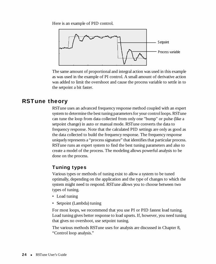
Here is an example of PID control.

The same amount of proportional and integral action was used in this example as was used in the example of PI control. A small amount of derivative action was added to limit the overshoot and cause the process variable to settle in to the setpoint a bit faster.

RSTune theoryRSTune uses an advanced frequency response method coupled with an expert system to determine the best tuning parameters for your control loops. RSTune can tune the loop from data collected from only one "bump" or pulse (like a setpoint change) in auto or manual mode. RSTune converts the data to frequency response. Note that the calculated PID settings are only as good as the data collected to build the frequency response. The frequency response uniquely represents a “process signature” that identifies that particular process. RSTune runs an expert system to find the best tuning parameters and also to create a model of the process. The modeling allows powerful analysis to be done on the process.

Tuning typesVarious types or methods of tuning exist to allow a system to be tuned optimally, depending on the application and the type of changes to which the system might need to respond. RSTune allows you to choose between two types of tuning.• Load tuning• Setpoint (Lambda) tuningFor most loops, we recommend that you use PI or PID fastest load tuning. Load tuning gives better response to load upsets. If, however, you need tuning that gives no overshoot, use setpoint tuning.The various methods RSTune uses for analysis are discussed in Chapter 8, “Control loop analysis.”

Setpoint

Process variable


Load tuningLoad tuning gives PI and PID tuning parameters optimized for load changes at the controller output. Load changes are the most difficult disturbances for the system to control. They are also the most common.There is always a tradeoff between fast response and sensitivity to changing process conditions. RSTune lets you further specify the type of load tuning you want to use, as well as a safety factor to control the sensitivity of load tuning.

Load tuning typesWith RSTune you can specify the type of Load Tuning you want to use.The three types of Load Tuning (with Safety Factor = 1) are:• Fastest:Optimal (minimum absolute error to load step)• Fast:Quarter amplitude damping• Slow:10% overshootThe fastest tuning with the lowest safety factor is the most sensitive to a changing process. Conversely, the slowest tuning with the highest safety factor is the least sensitive. The sensitivity of the loop can be analyzed using the Robustness plot, which is discussed in Chapter 8, “Control loop analysis.”

Load tuning with no overshootFor load tuning with no overshoot, decrease integral action in the fastest category by a factor of 3. For example, if your controller uses integral in time/rep, multiply the integral setting by 3. If integral is in rep/time, divide by 3. Setpoint tuning also gives you no overshoot.

Safety factorRSTune uses a safety factor to control the sensitivity of load tuning.The safety factor setting can be between 1.0 and 3.0. A setting of 1 means the tuning is very sensitive to small changes in the process but could become unstable if subjected to large or sudden load changes. A safety factor of 3.0 gives you conservative tuning; the loop will respond somewhat more slowly but is more stable when subjected to large or sudden load changes.More conservative tuning is appropriate in most situations, and 2.5 is the default setting. For faster response decrease the safety factor.

Tip You can use RSTune to help you design a setpoint filter. By using a setpoint filter you can get good response to both setpoint changes and load upsets. See Chapter 8, “Control loop analysis.”


If you enter a Safety Factor that might cause the system to be too sensitive, the message “Warning: Safety factor makes the loop dangerously sensitive to process changes” is displayed.You might then want to change the safety factor to a more conservative number, but this is only a warning. You can still download the more sensitive value.

Setpoint tuningSetpoint (or Lambda) tuning matches the setpoint response to a first order time constant (or lag time) that you enter. System response is first delayed by the process dead time. This method is popular in applications, such as in the paper industry, where overshoot is not acceptable. With Setpoint tuning the closed loop response should be the identified process dead time plus the target first order time constant (lambda time) you enter.

Caution Most control loops are somewhat non-linear. To be stable when the process changes, most loops require tuning with a safety factor larger (more conservative) than 1.


Chapter

Using RSTuneThis chapter provides you with information on the use of the basic windows of RSTune, including the menu commands, displays, display options, and button functions.These topics are covered:• Faceplate and Trend window• Changing the display of the Faceplate and Trend window• Using the Off Line Analysis & PID Tuning screen• Changing controller settings• Debugging communications• Menus• Creating a report for a control loop• Setting up extra trendsStep-by-step procedures are also provided in the online help system of the software.The details of control loop tuning using the methods available in RSTune are covered in Chapter 6, “Tuning control loops.”

Tip RSTune comes with a control loop simulation program that can be used to help you learn how RSTune works without being connected to a process. To use the control loop simulation:1. In the Choose a loop box in the Main window, click

Simulate.tun.2. Click Faceplate.3. See “Faceplate and Trend window” on page 28.

Using RSTune � 27

Faceplate and Trend windowThe Faceplate and Trend window is the screen where you begin the process of tuning and testing your control loops.The Faceplate and Trend window displays the process variable (PV), setpoint (SP), and controller output (CO) loop variables in a bargraph, as actual values, and in trend lines. Each is the same color in each display.

To display the Faceplate and Trend window:• From the main window: Double-click a loop in the Choose a loop list.• From the Setup window: Click Faceplate.The screen shown here is displayed.

Tip Controller output (CO) is sometimes referred to as the controlled variable (CV).

PV, CO, or SP display

Bargraph display

Menus

Buttons

Controller mode

PID parameter values(see units by hovering over values)

Span settings

Trend length in seconds

Real-time trend display

Arcchive On/Off Button


The Faceplate and Trend window includes:• Menus: Access options and features• Span settings: Allows changes to the way data is displayed• Archive On/Off Button: Allows you to turn the archiver on and off with

just the click of this button.• Real-time trend display: Displays real-time data from your processor• PV, CO, or SP display: If you hold the cursor over any point in the real-

time trend display, the PV, CO, or SP values at that time are displayed. The values that are displayed depend on the Span settings. See “Changing the value of the left and right axes” on page 31.

• Buttons: Perform various commands• PID parameter values: The current processor PID values and the new

values that will be downloaded to the process if Download is selected. • Controller mode: The current controller mode, auto or manual.• Bargraph display: Displays the loop variables in individual bargraphs and

boxes.

Changing the display of the Faceplate and Trend window

You can change the display of the Faceplate and Trend window to meet your needs.

Changing the Trend displayOn the Trend display, you can change:• How ticks are displayed• Whether the process variable, controller output, or setpoint span is used for

the right and left axes• Length of the trend (displayed as the horizontal axis of the real-time trend

display)To change how ticks and trend length are displayed:1. Select Options > Trend Options in the Faceplate and Trend window.

The Trend Options dialog box is displayed.

Using RSTune � 29

2. Click Help for a description of the options in this dialog box.

Changing the span, colors, and decimal placesThis window allows you to change display settings for the process variable (PV), controller output (CO), and setpoint (SP).To change how ticks and trend length are displayed:1. Select Options > Display Spans, Colors, Decimals in the Faceplate

and Trend window.

Tip You can also change these options by clicking the span button on the top left and right of the trend display).


This dialog box is displayed.

2. Click the tab for the parameter you want to change.3. Click Help for descriptions of the options in this dialog box.

Changing the value of the left and right axesYou can display the values for two variables (PV, CO, or SP) along the left and right vertical axes of the display. To change the value that is displayed, select the option you want from the Use dropdown at the upper right or left of the trend display.

Changing the display of the Faceplate and Trend windowYou can choose to display different combinations of the bargraph, trend display, and tuning information through the View menu. The view menu contains these options:• Faceplate Only• Faceplate & Trend• Faceplate, Trend & TuningA sample of what you will see for each selection is shown below.

Using RSTune � 31

Faceplate only

Faceplate & Trend


Faceplate, Trend & Tuning

Using the Off Line Analysis & PID Tuning screenIf you have archived data, you can work with RSTune offline. Offline tuning allows you to verify and edit data and calculate tuning parameters without opening the faceplate and going online.To work offline:1. Start at the main window.2. Select the loop you want to work with.3. Click Off-line. The Off Line Analysis and PID Tuning window is

displayed.From this window, you can:• Perform functions that are available in the faceplate when Tune From

Archived Data is selected. See “Using archived data” on page 50.• Use the Time Data Window by clicking Tune. See “Using the Time data

window” on page 57.• Set up a new loop using Options > Loop Setup.• Create a tuning report using Options > Tuning Report. See “Creating a

report for a control loop” on page 41.

Using RSTune � 33

Changing controller settingsThe setpoint, controller output, controller mode, and PID settings can be changed through the Faceplate and Trend window.

Changing the setpoint and controller outputWhen changing the setpoint, the value must be within the process variable spans of the loop.When changing the controller output, the value can only be changed when the processor is in Manual mode. The value entered must be between the controller output spans for the loop.To change the value of the setpoint or controller output in the Faceplate and Trend window:1. Double-click the Setpoint or Controller Output box.2. The Data Entry dialog box is displayed. Type the new value.3. Click Enter.

Changing the controller modeThe controller mode box below the bargraph allows you to change the controller mode. To change the mode, click the arrow and choose Auto (closed loop) or Manual (open loop).RSTune always displays the mode read from your controller. When you change modes, there is a slight delay before the new mode is displayed while RSTune writes the new mode to the controller and reads it back.


Debugging communicationsData Spy allows you to display raw data before scaling, formatting, or adjusting decimal points.Data Spy is available through the Faceplate and Trend window. To use Data Spy, select Options > Data Spy. This dialog box is displayed.

The Mode as ASCII chars box displays each character of the mode string as its ASCII value.The type of communications being used (DDE or OPC) is shown at the bottom of the dialog box.This window can remain open while other RSTune windows are active. It always stays on top.

MenusThe RSTune Faceplate and Trend window has four menu options:• Archive• View• Options• Help

Using RSTune � 35

Faceplate and Trend window options menuThis menu contains five choices.• Trend Options• Display Spans, Colors, Decimals• DDE Spy• Bring back Previous PID settings to New• Tuning Report

Faceplate buttonsThe buttons underneath the Trend window on the Faceplate allow you to choose to tune from previously archived data, use the AutoTune sequence, or close the Faceplate and Trend window.Descriptions of each of the buttons are included below. Detailed use of the buttons in various tuning functions is described in Chapter 6, “Tuning control loops.”

Tune from archived dataThe Tune from archived data button brings up a list of archived data files. (See Chapter 6, “Tuning control loops,” for information on collecting data.)

The list shows the name of the archive file, the date and time when the data was collected, and whether the file is an edited version of an archived file.To work with an archived file, click the filename.

Name of the original file (added by

“Yes” indicates that the file has been


The buttons below the archived file list are:• Tune: This button displays the Time data window. From this window, you

can have RSTune determine tuning parameters and perform analysis on the data. See Chapter 6, “Tuning control loops,” for details on using the Time data window.

• Copy to ASCII: This button allows you to save your data to an ASCII file (extension .asc). The file can be named and placed in any folder. You can also save the data as a print file (.prn) or as a data file in comma separated value format (.csv).

• Time Plot: The Time data window displays the process variable and controller output data. Use this window to verify that your data meets tuning requirements, or to edit data to optimize it before calculating new parameters.

• Delete: This button deletes the selected archived data file from your hard disk.

• Back: This button closes the archive data file list window.The Loop Notes box to the right of the archive list displays notes that have been entered concerning the loop. RSTune automatically adds notes to the Loop Notes when a file is edited. You can also enter notes manually by clicking Change Notes. To edit the Loop Notes for a data set:1. Select the data set.2. Click Change Notes.3. Type your changes in the Edit notes window.

4. Click OK to save your changes or Cancel to abandon them.

Tip Delete deletes the selected archived data file for the control loop, not the control loop. To delete the control loop file, see “Editing and deleting loops” on page 11.

Tip To start a new line in the Edit Notes window, press Ctrl + Enter.

Using RSTune � 37

AutoTuneAutoTune starts the AutoTune sequence. This is a sequence of questions that you can follow to have RSTune automatically calculate new PID tuning parameters for your control loop.The AutoTune sequence is described in “Using AutoTune to collect data” on page 45.

CloseThe Close button closes the Faceplate and Trend window and takes you back to the RSTune main window. It does not close RSTune.

Simulate windowWhen you open the faceplate for a loop with a processor type of “Software simulation,” the Simulate window opens minimized. This simulated control loop allows you to gain experience with RSTune without being connected to a processor.The loop simulator provides advanced simulation, including cascade and feedforward loops with multiple simultaneous simulations on the same plot for easy comparison.

The functions you can do from the basic Simulate window are listed here. For information on the Advanced button features, see “Advanced” on page 39.

Tip The information in the Simulate window is the same as the information on the Faceplate and Trend window, except for the Advanced button. Any changes to information in the Simulate window will also be changed in the Faceplate and Trend window.


AdvancedThe Advanced simulate window allows you to select one of seven process types and change the load.

If you select a non-linear process, characterizer information is displayed, as shown here.

To: Do these steps:

Change the setpoint, controller output, or PID values

Note: The controller output value can only be changed in Manual mode.1. Double-click the box.2. Delete the old value and type the new value.3. Click Enter.

Switch between Auto and Manual modes

Click the drop-down and select Manual or Auto.

Restore the initial tuning parameters

Click Initial PID. This option returns the initial tuning values, regardless of how many settings you have downloaded.This is different than the Bring back Previous PID settings to New option on the Faceplate and Trend window Options menu. The Bring back option restores only the previous PID values, not the initial values.

Using RSTune � 39

Descriptions of the options in the Advanced Simulate window are presented here.

To: Do these steps:

Display the Advanced Simulate window

1. Click Advanced from the Simulate window.2. Click No.

Change the process type

In the Process type dialog box, select the type of process. The diagram labels change to reflect the new process type. The trend display also shows the change.

Change the process load

In the Process Load dialog box, click +5% to increase the load or –5% to decrese it. The trend display on the Faceplate and Trend window shows the impact on the loop.

Experiment with Characterizer

When the Process Type is set to a non-linear loop, the Controller Characterizer dialog box is displayed.The Controller Characterize allows you to experiment with the Characterizer.Click Demo Instructions for more information on using the Characterizer in the Simulate window.For more information on the Characterizer (available only with RSProcess Perfector), see “Using the output Characterizer” on page 97.


Creating a report for a control loopYou can use the tuning report to create a record of the tuning results for a control loop. Reports can only be produced while tuning or for an archived data set (see “Using archived data files” on page 50 for information).RSTune creates reports in Microsoft® Word 97 with SR-1 or a higher version of Word. Word must be loaded to use the reporting feature.You can create a report while tuning or from archived data.To create a report:1. On the Faceplate and Trend window, select Options > Tuning Report.2. Wait while the report is being prepared. Doing other work on your

computer could interfere with the insertion of graphics in your report.3. Maximize Word to see the report.4. To save the report, select File > Save As in Word.

About the reportRSTune initially inserts these items when you create a report.• Current and new tuning values• Loop Notes• Time data window• PID Tuning Grid• Process model• Robustness Plot• Frequency Response (Bode) Plot• Simulation to Setpoint• Simulation to Load UpsetRSTune uses bookmarks in a Word template file to create the report.For information on using bookmarks and customizing the report, see the online help in RSTune and Microsoft Word.

Tip When you open the report in Word, you will see a message that tells you the document contains macros and asks what you want to do. If you disable macros, the document will open as read-only and you will be unable to edit it. You must select Enable Macros to open the report for editing.

Using RSTune � 41

Editing a reportOnce created, you can edit your report to be specific to your company.• Replace all occurrences of “Company Name” with your company’s name.

You can double-click on text in the headers or footers to edit it.• Change the letter on the cover page to suit your needs.• If using RSProcess Perfector, delete any blank graphs or data that you do not

want to use.• Edit or add notes on the graphics in the report.• Summarize your findings in the Conclusions and Recommendations.

Printing a reportTo print a report:1. Update the boxes by pressing Ctrl + A, then pressing F9.2. Select File > Print.

Setting up extra trendsYou can add an extra trend line to the Faceplate and Trend window. The Extra Trend variable must be in the same PLC as the loop.In RSTune, you can add one additional trend. This trend is for viewing (faceplate) only.If the Processor Type is set to Software Simulation, you will not see the Extra Trend on the Faceplate and Trend window.

Tip When you open the report, you will see a message warning that the document contains macros and asking what you want to do. If you disable macros, the document will open as read-only and you will be unable to edit it. You must select Enable Macros to open the report for editing.

Tip If archives have been collected for a loop, trends cannot be deleted and communication data cannot be changed. To delete trends or change communication data for a trend, either:n Delete the existing archives for the loop (see “Using archived data

files” on page 50 for information).n Create a new loop by clicking Save As in the Setup window.


To create a new trend:1. In the main window, click the loop that will contain the extra trend.2. Click Edit Setup. The RSTune Setup window is displayed.3. Click Advanced. The Extra Trends and Advanced Loop Setup dialog box

is displayed.

4. Click Extra Trends.The blank Setup Extra Trends window is displayed.

5. Click Add Trend. The Trend 1 tab is added, as shown here.

6. Set Eng span to the full engineering range of the trend variable.7. Set Inst span to the instrument range of the trend variable. This is the

range of the value reported to RSTune by the server.

Tip When RSTune reads Extra Trend values, it scales the values from the instrument span to the engineering span. If the value is not scaled, set Inst span to the same value as Eng span.

Using RSTune � 43

8. Set the display information. The options are:

9. Click Test. RSTune reads the variable from the server. RSTune displays the variable from the server or an error message.

Box Description

Description The name of the trend. This name is used on the Faceplate and Trend window. PV, CO, and SP cannot be used as names of extra trends.

Display span The range of data that will be displayed on the Faceplate and Trend window for this trend. The smaller the span, the higher the resolution on the display.

Decimal places The number of digits shown after the decimal point in the Extra Trend value displays. This only affects the display. Decimal places can be set from 0 to 5.

Line width The width of the trend line in the Faceplate and Trend window. Line width can be set from 1 to 4.

Line color The color of the trend line in the Faceplate and Trend window. To select a color:a. Click Line Color.b. Select the color.c. Click OK.


Chapter

Tuning control loopsRSTune makes analyzing, optimizing, and tuning control loops fast, accurate, and easy. You can simply follow an AutoTune sequence, or manually gather data and then have RSTune calculate the tuning parameters. You can edit the data to optimize the new parameters, and you can test the parameters without downloading them to your controller.You can tune data online or offline. Online tuning is done from the Faceplate and Trend window. Offline tuning is done from the Offline Analysis and PID Tuning window, which is selected by clicking Offline in the main window.These topics are covered in this chapter:• Collecting data• Using AutoTune to collect data• Manually collecting data• Using archived data files

Collecting dataWith RSTune, you can follow the AutoTune sequence to determine PID tuning parameters, or you can manually gather data and tune using that information.

Using AutoTune to collect dataAutoTune prompts you to gather data. RSTune uses the data to calculate new PID tuning parameters for your control loop.AutoTune can be done with the controller in either Manual or Auto mode. If the controller is in:• Manual mode: The controller output is changed• Auto mode: The setpoint is changed

Tuning control loops � 45

When gathering data:• Collect the process variable and controller output data from a step or pulse

test. You can make a setpoint change (in Auto) or a controller output change (in Manual).

• Both the process variable and controller output must start and end at a steady state condition and include the complete response to the setpoint or controller output change. When steady state out, both the process variable and controller output are relatively flat horizontal lines in the Trend display, moving within the range of normal process noise.

• RSTune analyzes process variable and controller output data pairs.• All process variable filtering must be removed from the signal.

When you use the AutoTune sequence, data is automatically archived.

To AutoTune:1. From the main window, click the loop to tune.2. Click Faceplate.3. Click AutoTune. The lower left part of the window changes as shown

here.

If your loop is erratic or cycling, try:� Putting the loop in Manual and waiting for it to settle out.� Putting it in Auto mode and entering a low proportional gain and a low

integral gain. Wait for the loop to settle out.

Caution The data must not be from a load or process upset. Loads must not change during the test and the range of test data should be as linear as possible. If a load change occurs during the test, click End Sequence and begin the test again.

Tip You can stop the AutoTune sequence at any time by clicking End Sequence.


4. When your process data is steady state, click Yes. The screen shown here is displayed.

5. RSTune needs to produce a bump in your process by making a setpoint or controller output change. The default is 7.To use a different value, click Different. You are prompted for a value. You can use negative numbers if needed. Click Enter.

6. Click OK.7. If the loop is in Auto mode or you are tuning a simulated loop, go to the

next step.a. If the loop is in Manual mode, this prompt is displayed.

b. If you click Yes, this screen is displayed.

To get good data for tuning, RSTune needs to see the process variable respond to the controller output. The amount of process variable response needs to be at least 4 to 6 times larger than the normal peak-to-peak noise in your process.

Tip If you are using the Simulate.tun file that comes with RSTune, you might want to use a larger value. The default is not much larger than the process noise, so you will get better data if you use 10 or 15.


c. After the process variable moves by this amount, click Yes. RSTune changes the controller output back to its original value.This dialog box is displayed.

8. When the process has steady state, click Yes.9. The name of the archive file for this data is displayed. Click OK.10. The Time data window for the data is displayed (see Chapter 7, “Using

the Time data window”). You can start verifying or editing your data and determining new PID tuning values.

Manually collecting dataRequirements for gathering valid data:• Collect the process variable and controller output data from a step or pulse

test. You can make a setpoint or controller output change.• Both the process variable and controller output must start and end at a

steady state condition and include the complete response to the setpoint or controller output change.

Collecting data manuallyIn some cases, you might want to collect data manually instead of using the AutoTune sequence. This is a basic procedure to collect data manually. This is a closed loop test with the controller in the Auto mode.

Caution Plant data taken for RSTune analysis and tuning must have all process variable filters removed from the signal.

Important The data must not be from a load or process upset. Loads must not change during the test and the range of test data should be as linear as possible. If a load change occurs during the test, stop collecting data and start over.


Examples of other methods of collecting data manually are provided in Chapter 9, “Application notes.”To collect data manually:1. Make sure the controller output is not at 0%, 100%, or saturated into a

limit. If it is, change the controller output to between 5% and 95% (or not at a limit). Valves are usually non-linear at their limits.

2. Let the loop settle out (reach steady state).3. Select Archive > Archive On.4. Change the controller setpoint by about 10%.5. Wait for the process variable to respond an appreciable amount, then

change the setpoint back to its original value. Skip this step if your process can tolerate a new operating point.

6. Let the loop settle out (reach steady state).7. Select Archive > Archive Off.

Data pair and sample interval requirementsTo get valid data for tuning and analysis:• The total points used for analysis must be at least 33 and not larger than one

billion• If there are more than 1025 data pairs (process variable and controller

output), RSTune compresses the data to 1025 pairs.• Very high quality tuning can be determined with between 200 and 500 points

of data.If the data is compressed, the quality of the analysis and tuning might be poorer if the loop has a small equivalent dead time compared to the data sample interval. Equivalent dead time is the amount of time that it takes for your process variable to start changing appreciably after the controller output changes.Data should be collected with a sample interval that is at least 4 times faster than the equivalent dead time of your process. If it is not, RSTune displays a message stating that, for optimal tuning, the sample interval should be smaller.


Using archived data filesRSTune allows you to store data in archived data files that you can use to:• test your loop• prepare for manual tuning• calculate tuning parameters• perform “what if” analysis• verify and edit data• copy to an ASCII fileYou can also add notes to the archived data.

Archiving dataData collected with the AutoTune sequence is automatically archived.You can also manually archive data:1. Select Archive > Archive On.

RSTune starts archiving data to a file with the same root as the .tun file.2. When you are done collecting data, select Archive > Archive Off.When you turn archiving on, RSTune displays the name of the file where the data is archived in the title bar of the Faceplate and Trend window:

Using archived dataOnce archived data is collected, you can display it in the:• Faceplate and Trend window: Click Tune from archived data.• Off Line Analysis and PID Tuning window: In the main window, click

Offline. The Offline button is available after data has been archived.The list of files looks like this in the Faceplate and Trend window:

Tip See online help for rules on archive file naming.


It looks like this in the Off Line Analysis and PID Tuning window:

Tuning from archived dataTo tune from archived data:1. Click the archived data file name.2. Click Tune.

The Time data window and the new tuning parameters are displayed.3. Verify or edit the data.4. When you are done tuning the data, click Back or Done Tuning.

For information on using the Time data window, see page 57. For information on calculating and using new tuning parameters, see page 59.

Deleting archived filesTo delete an archived file, select the archived data file name. Click Delete. The remaining data files will not have their file extensions renumbered.

Adding notes to an archived data fileThe Loop Notes box to the right of the archived data files displays notes about the selected file. RSTune adds notes automatically when a file is edited and saved. You can also add notes manually.To add notes to a file:

Tip The Time and Date shown in the “When collected” box indicate the time and date when the archive was started.

Tip This function does not delete the Control Loop file. See “Editing and deleting loops” on page 11 for information on deleting a control loop.


1. Select the file from the list. Any existing loop notes are displayed.2. Click Change Notes. The Edit Notes window is displayed.3. Type your notes in the Edit Notes window.

4. Click OK.

Saving archived data to a different formatArchived data files can be saved to an ASCII (.asc), printer (.prn), or comma separated value (.csv) file.To save the data in one of these formats:1. Select the data file.2. Click Copy to ASCII.

The Save Data to ASCII File dialog box is displayed.3. In the File name box, type the file name for the file.4. In the Save as type box, select the file type.5. Click Save.An example of an ASCII file is shown here.

Header Section

==============

Number Of Header Items: 40

Scan Interval: 1

Time Stamp Units: milliseconds

Number Of Channels: 3

Date/Time Data Collected: 10/16/97 11:06AM

Version: 9.06.16

Who Created Me: RSTune

Current P: 2

Tip To start a new pargraph in the Edit Notes window, press Ctrl + Enter.

Tip Only a small portion of the information that is available is shown in this example. Depending on the number of trends created and the amount of archived data colleetd, you will normally see more information.


Current I: .58333

Current D: 0

Current F: 0

Channel 1 Description: PV

Channel 1 Eng. Min. Span: 0

Channel 1 Eng. Max Span: 100

Channel 2 Description: CO



Channel 3 Description: SP



Response Direction: up

Controller Algorithm: Allen Bradley PLC-5 PD fileISA, D on PV

Controller Type: ideal

PB Or Gain: gain

Integral Units: min/rep

PB Multiplier: 1

Integral Multiplier: 1

Derivative Multiplier: 1

Mode: 1

PID: 4

TimePlot AutoScale PV: 0

TimePlot AutoScale CO: 0

TimePlot PV Min: 41.63655

TimePlot PV Max: 49.87732

TimePlot CO Min: 39.31247

TimePlot CO Max: 55.48609

TimePlot Number of Lines: 0

TimePlot Line Position1: 0

Timeplot Line Position2: 0










Timeplot Line Position Hyst1: 0




Characterizer Fit Type: 0

Characterizer Language: 0

Characterizer Lines: 0

Characterizer Blue Y1: 0

Number Of Points: 192

ArchiveNotes: Data collected manually with thecontroller in Auto mode.

Data Section

============

PV CO SP

----------- ----------- -----------

41.46768 39.78901 42

41.30512 40.99653 42

41.62125 41.36135 42

41.5027 39.8148 42

41.64124 40.96721 42

41.89695 38.49328 40.85577

42.13604 31.08119 37.29519

42.30678 25.70074 35

42.32682 24.43569 35

42.26803 23.97164 35

41.42966 23.6704 35

39.54797 25.02115 35


Changing and downloading PID parameters to the controllerThe PID values can be changed through the Faceplate and Trend window. The values can be changed manually or you can have RSTune calculate them automatically using the options described in “Controller tuning” on page 61. When the values are correct for your system, they can be downloaded to the controller.To change the values manually:1. Click the New box of the parameter you want to change.2. Delete any existing characters.3. Type the new value.4. You can now download the values as described below.

Downloading PID parameters to the controller

To download the new PID parameters to the controller or the software simulation:1. Click Download on the Faceplate and Trend window.

2. This window is displayed.

3. Click Yes.

Caution Downloading different gain values while the processor is in the Run or Remote Run mode might cause unexpected machine operation, which can result in injury, loss of life, or machine damage.

Tip Download is not available if you are tuning from the Offline Analysis and PID Tuning window.


After the values are downloaded, the Current and New parameters are the same.

Retrieving previous PID settingsTo check what the PID settings were before the download, you can use the Bring Back Previous PID Settings to New option. When you select this option, the New settings are replaced with the settings that had been in the Current column before the download.To retrieve the previous values, select Options > Bring back Previous PID settings to New. The values under New are changed to the values that were in Current before the download. These values can be downloaded.


Chapter

Using the Time data windowThe Time data window displays the process variable and controller output data. Use this window to verify that your data meets tuning requirements, or to edit data to optimize it before calculating new parameters.This window is displayed when:• The AutoTune sequence is complete• You select an archived data file and click Tune• You are in the Offline Analysis and PID Tuning window and click Time

Plot or TuneThis window can be moved anywhere on your screen and remains on top of other RSTune windows. An example Time data window is shown here .

These topics are covered in this chapter:• Changing the Time data window display• Calculating tuning parameters• Controller tuning• Editing data in the Time data window• Verifying data using the Time data window

Using the Time data window � 57

Time Data ToolbarThe toolbar is located near the top of the time data window.

Tip Before working with data, it might be helpful to review the section “Data pair and sample interval requirements” on page 49.

Button Menu Command Description

Tune Button on Faceplate Calculate Tuning

Zoom>Zoom In Zoom In

Zoom>Zoom out to see all data Zoom out to see all data

Edit>Average Average

Edit>Line edit Line Edit

Edit>Filter Fiter

Edit>Undo Undo Changes

Options>Statistical Analysis Statistical Analysis

Options>Hysteresis Check>Automatic Hysteresis Check (automatic)

Options>Report>Full Tuning Report Full Tuning Report


Changing the Time data window displayYou can change the line weight and type of graph that is displayed.

Changing line weightSelect Options > Thick Lines to make the lines in the graphs thicker. Click it again to make the lines thinner.

Changing the graph typeYou can display the Time data window to a bar graph. Select Options > Plot As Bars. Select this option again to switch it back.

Calculating tuning parametersYou can calculate tuning parameters when the Time data window is displayed. The Time data window is displayed:• upon completion of the AutoTune sequence• from the faceplate when you click Tune from archived data, select a data

file, then click Tune• from the Offline Analysis and PID Tuning window when you select a data

file, then click TuneWhen the Time data window is displayed, RSTune calculates and displays New PID parameters for the control loop. It also adds the Controller Tuning, Probable Performance Increase (or Are Current Settings Stable), and Analysis options to the Faceplate and Trend window.


The PID parameters are based on the data collected for your loop. Before the loop is tuned, the New column displays N/A (Not Applicable) for each parameter. The parameters in the New column are recalculated as you make changes in the Controller Tuning section of the Faceplate and Trend window and as you make changes to data in the Time data window.You can also change any of the New tuning parameters yourself. Click the box of the parameter you want to change, edit the value, and press Enter.The Probable Performance Increase is updated as the PID parameters change and tells you how much better the controller will respond to a load upset with the new PID parameters. It is the percent probable performance increase in integrated absolute error (IAE) to a load upset assuming the controller does not overshoot to a load upset with either the current or new parameters. If the controller overshoots, the performance increase is an approximation that is roughly proportional to the IAE improvement. It is still a good predictor of performance.This box says None if the Probable Performance Increase is insignificant. Adding derivative might increase the performance in these cases. (Click the Use derivative if possible box.)

New PID parameters and probable performance increase or are current settings stable message

Controller tuning selections

Analysis button(see how good your data is by hovering over this button)


To determine the optimal tuning parameters for your loop:• Verify and edit your data using the Time data window (below).• Select the desired tuning factors in the Controller Tuning section of the

Faceplate and Trend window (below).• Analyze the effects of the new PID parameters using the Analysis windows

(Chapter 8, “Control loop analysis”).

Controller tuningWhen the Time data window is displayed, you can select the controller tuning factors that you want to use for this loop.

To select controller tuning factors:1. From the:

� Faceplate and Trend window: Click Tune from archived data. Select a file and click Tune.

� Offline window: Click Tune.The Time data window is displayed and the Controller Tuning section is added to the Faceplate and Trend window, as shown here.

1. Pick the type of tuning you want to use:� Load Tuning - Fastest: Recommended for most loops. Provides

minimum absolute error to step load.� Load Tuning - Fast: Provides quarter amplitude damping.� Load Tuning - Slow: Provides 10% overshoot.� Setpoint Tuning: Provides good setpoint response at the expense of

good regulation.

Tip See Chapter 4, “Tuning theory,” for definitions of load tuning, setpoint tuning, safety factor, and other RSTune parameters.

Tip To see what the PID settings would be for each type of tuning, click PID Grid were you will be able to change the settings and see the effects in one window.


2. For:� Load Tuning: Type a Safety Factor between 1 and 5, with 1 being the

most sensitive.� Setpoint Tuning: Type a Response time (in seconds). For a faster

response time, use a smaller response time. For slower response, use a larger response time. The default value that RSTune sets is conservative to prevent overshoot on setpoint change.

3. To use derivative gain, select Use derivative if possible.4. Click Done tuning. The Time data window closes. If you are using the

Off Line Analysis and PID Tuning window, the PID parameter display is also closed.

Editing data in the Time data windowData in the Time data window can be zoomed, averaged, edited by line, and filtered.After you edit the data, RSTune automatically recalculates and displays the PID tuning based on the changes.

ZoomingAfter collecting data, you might want to zoom in on the data you want to use for tuning. This is typically the smallest window of data that starts at a steady state condition and ends within about 5% of steady state. You can zoom manually or use Auto Zoom. When Auto Zoom is used, RSTune automatically tries to zoom in on the data that offers the best tuning.

Zooming manuallyTo zoom in on your data:1. Select Zoom > Zoom in.2. Click the graph where you want to begin zooming.3. Click again where you want to end zooming. The portion of the graph you

selected is highlighted.


4. To change the zoomed area, click at the new spot. You can do this as many times as needed. Clicking the graph anywhere to the right of the midpoint moves the right edge of the highlighted area. Clicking to the left of the midpoint moves the left edge.To include all of the data points to the left, click just outside the left side of the graph. To include all of the data points to the right, click just outside the right side of the graph.To stop zooming, click Cancel Zoom.

5. Click Zoom Now.You can zoom in as many times as needed.To return to the previous view, select Zoom > Zoom Back to Previous.To return to the view of all data, select Zoom > Zoom Out.

Using Auto ZoomTo use Auto Zoom:1. Select Zoom > Auto Zoom. The data is highlighted.2. Click Zoom Now to accept the data.Auto Zoom attempts to zoom based on the current data. If RSTune does not have the proper data to perform Auto Zoom, the error message “Cannot automatically find a zoom location in the data” is displayed. You can then either zoom manually, or recollect data and retry Auto Zoom.


Averaging dataRSTune uses your initial data as the steady state basis for all tuning and modeling. Ideally, this data should start and end at steady state. However, if your initial data is noisy or cycling, averaging might improve your tuning results. Average the controller output and the process variable data to just where it starts changing due to the bump introduced as part of the test.To average a portion of your data:1. Select Edit > Average.2. Click the beginning point of the data you want to average.3. Click the end point of data you want to average. That section of data is

highlighted.

4. To change the area, click at the new spot. You can do this as many times as needed. Clicking the graph anywhere to the right of the midpoint moves the right edge of the highlighted area. Clicking to the left of the midpoint moves the left edge.To include all of the data points to the left, click just outside the left side of the graph. To include all of the data points to the right, click just outside the right side of the graph.To stop averaging, click Cancel Avg.

5. To modify your data, click on the graph at the new beginning or end point of the data you wish to average.

6. To accept the change click Avg now.You can undo the last averaging operation. Select Edit > Undo.

Setpoint

Process Variable


Changing data points to a lineThe line edit option allows you to change a series of data points to a line between two points you select. This is useful for removing any noise spikes or other spurious data from your graph.To do this:1. Select Edit > Line edit.2. Click the beginning data point you want to edit.3. Click the point where the line should end.4. RSTune changes the data to be a line between the two points you picked.5. You can edit as many data points as needed.

6. Click OK.To undo the line editing session, select Edit > Undo.To filter your data:1. Select Edit > Filter. This window is displayed.

2. Select the Filter type from the list. For filter descriptions, see the online help.

3. Type the Filter time constant in seconds. Pick a filter time large enough to eliminate as much noise as possible without degrading loop performance. If the filter time constant is too large, it can hurt loop performance, because the control system will try to control the filter.

Noise spikes have been edited into a line.


4. Click Test to test the effects of filtering. The graph in the Time data window is redrawn with the filter values applied.

5. Click OK to accept the filter values or Cancel to ignore the changes.To undo the filtering change, click Edit > Undo.

Saving changesAfter making editing changing in the Time data window, you can save the changes by selecting Edit > Save changes. The edited data is automatically saved in a new archive data file. RSTune keeps both the original and the edited data file or files. The edited file is indicated by “Yes” in the Edited column. RSTune automatically adds a note that identifies the original file.

Verifying data using the Time data windowUse these tools to verify data:• Statistical analysis• Hysteresis check• Hysteresis check

Statistical analysisStatistical analysis can be used to check the improvement in control with the new tuning parameters. Before tuning, collect the normal operating data (with no setpoint changes) with the controller in Auto. Download the new tuning parameters and collect normal operating data again. Compare the statistics for both sets of data.

Caution Filtering modifies your plant data. If you use the filter, subsequent tuning will be based on the filtered process variable.

The file that the edited file was created from.

Yes indicates that data in this file was edited.


After you gather data for statistical analysis:1. On the faceplate, select Tune from archived data.2. Select the file to analysis.3. Click Tune. The Time data window is displayed.4. Select Options > Statistical Analysis. This window is displayed

The Time data window also changes to show the statistics as mean, standard deviation, and 2x standard deviation lines on the process variable graph.

Definitions of the statistics are:• Sample (raw): The data collection sample interval in the archive.• Mean (µ): The average of your data.

Tip Be sure to turn Archiving on when collecting data so you can save and compare the two sets of data. Select Archive > On to start archiving. Select Archive > Off when data collection is complete.

Mean (red line)

Standard deviation (blue lines)

2x Standard deviation (green lines)


• Standard Deviation: The square root of the sample variance.

• Sample Variance: The spread or dispersion of your data.

• Variability: The relative value of variance. It is expressed as a percentage of the mean, allowing comparison between the level of variability in different processes.

• IAE - Integrated Absolute Error. Performance of a loop is judged by how closely the controlled variable is held to the setpoint, both for setpoint changes and load changes. There are many mathematical ways of judging this, and IAE is one type. IAE is a measure of controller error defined by the integral of the absolute value of a time dependent error function.

Hysteresis checkRSTune can perform a hysteresis check on your data. Hysteresis is a dead band in the movement of a device upon a change of direction.For example, if a valve is moving in one direction, it continues to move if the air signal keeps moving in the same direction. But when the air signal changes direction, the valve has to stop and reverse motion. Conditions like static friction take time to overcome. This time, or hysteresis, must be compensated for by the air signal increasing to an amount equal to the hysteresis before the valve will move in the other direction.If RSTune cannot calculate hysteresis from your data, an error message is displayed. Click Yes to this message to display information on how to properly gather data to perform a hysteresis check.If your hysteresis is more than 1% for valves with positioners or 3% for valves without positioners, consider repairing or changing equipment to try to reduce the hysteresis.

Collecting data for a hysteresis checkThe hysteresis check requires several controller output changes while the controller is in Manual mode: two steps in one direction and one step in the other. To collect data for a hysteresis check:

mean sum of your measurement datanumber of data points

------------------------------------------------------------------------=

standard deviation sample variance=

sample variancemean x i( )–( )2

�number of data points 1–------------------------------------------------------------=

variability 100 2 standard deviation( )×mean

-----------------------------------------------------------------=


1. In the Faceplate and Trend window, select Manual mode. 2. Select Archive > On.3. Wait for the process variable to settle out and collect a little more data to

get normal process noise.4. Increase the controller output by 5%.5. Wait for the process variable to settle out.6. Increase the controller output by another 5%.7. Wait until the process variable settles out.8. Decrease the controller output by 10%.9. Wait until the process variable is at steady state.10. Click Archive > Off.

Performing the hysteresis checkOnce the data has been collected, you can do the Hysteresis check:1. Click Tune from archived data.2. Select the archive file collected above.3. Click Tune. You might see a message indicating that the data is

questionable for tuning. You can ignore this, as it does not reflect on the data’s suitability for a hysteresis check. Click OK.

4. To check:� Automatically: Select Options > Hysteresis check > Automatic.

5. The time data graph changes as shown here.


The areas RSTune used to calculate hysteresis are indicated on the graph. RSTune finds each of the three areas where steady state occurred in the process variable after a step change. The areas are:� p2: From the first steady state area to the second� p3: From the second steady state area to the third� A magenta line is drawn at the noiseband minimum and maximum

values.The controller output graph is labeled at each step change (C1, C2, and C3). If the controller output data is noisy, average the data to make it clean between steps (see page 64).

Notes on the hysteresis checkDuring the hysteresis check, information is displayed on valve sizing and transmitter span. Process gain that is too high could be an indication of incorrect valve sizing, incorrect valve characteristic, or a transmitter span that is not correct for the loop. If any of these items are incorrect, the loop can be difficult to control, and usually results in a cycling loop.

Valve oversizedAn oversized valve cannot provide very fine control. Any valve has a rangeability factor that determines how precisely it regulates. A good control valve might have a rangeability of 100 to 1, which means you can make 1% adjustments in the output. The valve can also be referred to as having a resolution of 1%. This allows finer control with less chance of inducing hunting or cycling.If a valve is oversized, the usable operating range of the valve gets smaller. For example, a valve with a rangeability of 100 to 1 could be oversized for an application to the point that its effective usable operating range is only 50 to 1 (process gain of 2). This translates to a resolution of 2%.The oversized valve can only be adjusted within 2% instead of 1%. It no longer has tight control, and the process might be hunting within the valve resolution. The oversized valve could also be operating on its seat. A command could be sent to the valve, but it might not move off its seat since control isn’t precise.The solution to an oversized valve is to change the valve trim or replace the valve with one of the appropriate size.

Valve undersizedAn undersized valve can be a safety problem since it might not have the range to control the process. The solution to an undersized valve is to change the valve trim or replace the valve with one of the appropriate size.


Transmitter span too largeThe most likely reason for the process gain to be larger than 3 is if the process variable transmitter span is larger than it needs to be. The resolution of the measurement improves with a smaller transmitter span.The resolution of your measurement is the smallest change that your system can detect.For example, you have a choice of two transmitters connected to a controller. The controller has a 12-bit analog to digital converter with a resolution of 1 in 4096 (212 = 4096). Converted to percentage: 1/4096 = 0.0002441 ≈ 0.024%.

You are measuring temperature and one of the transmitters has a span of 0 to 4096. With the 12-bit converter described above, you are only able to measure and control within 1 degree: 4096 * 0.024% ≈ 1The other transmitter has a span of 100 to 500 degrees. Your resolution would improve: 500 – 100 = 400 400 * 0.024% ≈ 0.1Now your system could detect a change of 0.1 degrees instead of 1 degree.If you only need to detect and control a measurement within a certain range, choose a transmitter span that represents what you need.

Transmitter Span Too SmallThe gain of the loop might also be large if the transmitter span is too small or too narrow. The solution is to widen the span. You are more likely, however, to encounter transmitter spans that are too large than too small.

Adding data from the Time data window to the reportTo add data from the Time data window to the report, select either:• Options > Report > Full Tuning Report: Generates the full tuning report.• Options > Report > Just Add This to Report: Places this graphic in the

tuning report for this loop.See “Creating a report for a control loop” on page 41 for more information on reporting.

Controller A/D

Resolutionof 0.024%

Span of 100 to 500Resolution of 0.1 degree

Span of 0 to 4096Resolution of 1 degree



Chapter

Control loop analysisRSTune provides advanced analysis tools that you can use to test your tuning parameters before downloading them to the controller. Five of the analysis tools are available by clicking Analysis on the Faceplate and include:• Process Model• Process Frequency Response Plot• Control Loop Simulation Plot• Robustness PlotThese tools can be used to do “what if” analysis of your tuning parameters before you download them to the controller.

Using the standard analysis toolsTo use the Process Model, Process Frequency Response, Control Loop Simulation, and Robustness plots:1. Open the Faceplate.2. Click Tune from archived data.3. Select the archive file to tune.4. Click Tune. The Time data window is displayed.

Tip The quality of the information in the analysis windows depends on the quality and relevance of the data that you collected. RSTune models are based on frequency response. Frequency response is based on the data shown in the Time data window.

Control loop analysis � 73

5. Click Analysis.All four analysis plots open.

6. Begin working with the plots by selecting a model from the Process Model window.

Selecting a process modelThe Process Model window shows the process model type identified for your control loop. RSTune uses your process frequency response to identify the model as first order or second order.

Analysis button(see how good your data is by hovering over this button)

Tip If you close one of the analysis windows, all of the analysis windows close.When you change a PID tuning value, the Control Loop Simulation and Robustness plots update immediately. (See “Robustness plot” on page 80 for information on the Robustness plot.)

Tip The quality of your models, simulation, and robustness depend on the quality and relevance of your time data.


To select a process model:1. Adjust the plot windows so that you can see the Process Model, Process

Frequency Response, and Robustness Plot.2. Check the data on the Process Frequency Response and Robustness

Plots.3. In the Process Model window, select the other Model type from the list

(Force steady state gain or Allow gain to float). The plots change to reflect the new model.

4. Check the data on the Process Frequency Response and Robustness Plots.

5. In the Process Model window, select the Model type that fits your data the best.

6. Once you’ve determined the best Process Model, you can use the Process Simulation window and the Robustness Plot to analyze the calculated and current PID parameters.

Tip The Process Frequency Response plots both the actual and the model data. Choose the model that is closest to the actual data of Amplitude Ratio and phase. The most important frequencies are where the phase is between about 90 and 180 degrees (phase lead) or –90 and –180 degrees (phase lag).The Robustness Plot shows the trade-off between tight tuning and sensitivity to process changes. If you have two sets of tuning with about the same robustness, you can generally choose the faster response.


Options in the Process Model window

The table in this window shows the gain, dead time, and time constant values for the selected Model type. If RSTune identifies the model as second order, you see two Time constant entries in the table: 1st Time constant and 2nd Time constant. If your process type is integrator, the first order time constant value displays the word integrator. (The integrator process is discussed more in Chapter 9, “Application notes.”) If the model is second order and the roots are imaginary, the time constant displays the word imaginary.

Model TypeAll of the analysis windows depend on the model type chosen. Two models are available. When you choose a different model, all the analysis windows update. The model types are:• Allow gain to float: Causes RSTune to ignore steady state information and

fit the model based on higher frequencies. These higher frequencies are more important to optimal and stable closed loop control.

• Force steady state gain: Forces the steady state gain to be equal to the amplitude ratio at the lowest frequency. The model is fit using the remaining good frequencies. The lowest (or zero) frequency values for amplitude ratio and phase are not plotted on the frequency plot, so at the lowest plotted frequency, the model frequency response might not appear to match the process.

If you selected the Inverse Response option in the Advanced window during loop setup, the model will also show a lead time and integrator.

Starting the SimulatorThis option is available by selecting Options > Start Simulator With This Model. This starts the simulator using information from the selected model. For more information on the Simulator, see “Simulate window” on page 38.


Process Frequency Response (Bode) plotThe Process Frequency Response plot (also known as a Bode plot) shows both the actual and the model process frequency responses for comparison. Actual process data usually is noisy or jittery at higher frequencies (toward the right). Use this plot to help you determine which process model is best. In general, you want the closest fit at frequencies where the phase is between about 90 and 180 degrees.RSTune uses the data in this plot to calculate new PID tuning parameters.

The left vertical axis is the scale for the amplitude ratio in decibels. Two plots of amplitude ratio are provided, one based on actual data and the other based on the Model type.The right vertical axis is the scale for phase angle in degrees. Two plots of the phase angle are provided, one based on actual data and the other based on the Model type.The amplitude ratio and phase angle are plotted against frequency in radians/time (logarithmic scale) on the horizontal axis. The lines are color coded.The process frequencies most important to process control are those between about 90 and 180 degrees of phase.In Process Frequency Response plots for first order time constants, the corner frequency (or cut-off frequency) is where the amplitude ratio starts to turn and the phase lag equals 45 degrees. Consider a sine wave input to a process at this corner frequency. The output of a first order process has half the input power at the corner frequency.


A lag time or first order time constant of 10 has a corner frequency of 1/10. A PID controller with an integral time of 10 also has a corner frequency of 1/10. A PID controller with a derivative time of 10 has a corner frequency of 1/10; however, for derivative, this represents a phase lead of 45 degrees rather than phase lag.To find these frequencies:1. Look at the red scale on the right of the plot. Locate –90 and –180.2. Find the stretch of the red phase angle line between –90 and –180. These

are the most important phases.3. See where the –90 and –180 phase points line up vertically with the blue

amplitude ratio line. These are the most important amplitude ratios.The Process Frequency Response plot is based on process data only, and therefore does not update if the PID tuning changes. It only updates when the Model type changes.The Options menu on the Process Frequency Response window allows you to:• Display the plot in Radians/sec. This is the default.• Display the plot in Cycles/sec.• Show High Frequencies. With this option checked, RSTune shows

amplitude ratio and phases for frequencies with phases lower than –270 degrees.

Control Loop Simulation plotThe Control Loop Simulation plot shows you a simulated response so you can see how the loop will respond before downloading tuning parameters. Use this plot to perform “what if” analysis on your control loop by trying different settings and checking the response.This shows setpoint response and response to a process upset. Setpoint responses and process upset responses can be very different. Normally, you can’t easily test your plant with process upsets, but RSTune can show you the simulated response. Reducing or eliminating process upsets is generally more important to product quality and waste reduction than setpoint response.The Control Loop Simulation plot allows you to simulate the entire loop and do valve wear analysis through a:• Set point plot• Load plotIt also allows you to compare the actual process variable to the simulated process variable.


If you change the model of your process, or change a PID tuning parameter, the simulation is instantly recalculated to reflect your changes.All of the plots show the response for both the current and new PID parameters for comparison. New PID parameters are shown in red and current parameters are shown in blue.

Options in the Control Loop Simulation plotThe options in the Control Loop Simulation window are:• Options > Thick Lines: Makes the plot easier to read.• Time Range > Expand or Shrink: The scale on the Control Loop

Simulation is initially set by RSTune. To increase the scale, select expand. To decrease the scale, select Shrink.

Setpoint plotThe Set Point Plot shows the response to a setpoint change for the current settings and the new settings.This is the first plot displayed if you selected Set Point tuning on the Faceplate. If it is not displayed, you can select it using Options > Set Point plot.A setpoint plot is shown here.

Load plotThe Load plot shows a simulation of a process upset. RSTune applies a step load change to the simulation.This is the first plot displayed if you selected Load Tuning on the Faceplate. If it is not displayed, you can select it using Options > Load plot.This example shows the response to a process upset. The upper portion of the window shows the process variable response and the lower portion shows the controller output response.


Robustness plotThe RSTune Robustness plot shows how sensitive your loop is to process gain or process deadtime changes. The Robustness plot graphically shows the tradeoff between tight tuning and stability. If you have two sets of tuning parameters with about the same robustness, you can generally choose the faster response. An example Robustness plot is shown here.

The two axis of the plot are process gain and dead time.The plot has a region of stability and a region of instability. The red (new tuning parameters) and blue (current tuning parameters) lines on the robustness plot are the limit of stability. To the right and above the lines, the closed loop process is unstable. To the left and below the lines, the closed loop system is stable.The crosshairs in the safety factor area are at the actual process gain and deadtime. Generally, a safety factor or divisor of 2 is reasonable for a control loop. For practical system stability, keep the limit of stability line outside the safety factor area.

New

Safety factor area. The plots should be outside of this region (above and to the right)

Current


For example, in the Robustness plot shown above, the line for the current tuning parameters is inside the safety factor area. These parameters offer very tight tuning, but if the system encounters a high gain ratio, it will be in the region of instability. The line representing the new tuning parameters is well outside the safety factor area, offering more stability.Robustness plots are calculated using the Process Model and controller tuning values. The accuracy of the plot depends on the accuracy of the model.Whenever you choose a different model in the Process Model window, the Robustness plot refreshes. This plot also updates when a new Safety Factor value is entered on the faceplate.RSTune conservatively estimates process dead time when dead time gets close to the sample interval. If your plant has very small dead time, the model appears less stable and the verge of stability lines is lower. The simulations (which use the model) also appear less stable than your plant.

Options in the Robustness plotThe options in the Robustness plot are:

• Actual Gain and Dead Time• Gain and Dead Time Ratio• Robustness Increase• Closest Distance

Actual Gain and Dead TimeYou can display the Robustness plot with axes of gain and deadtime.To display this plot, select Options > Actual Gain and Dead Time.

Gain and Dead Time RatioThis changes the plot to show Dead Time Ratio and Gain Ratio. To display this plot, select Options > Use Gain and Dead Time Ratio.The gain ratio is:

The deadtime ratio is:

At the cross, where both ratios are 1, the process gain and deadtime are at the process values you tuned for.

gain ratio process gainprocess gain the controller was tuned for-----------------------------------------------------------------------------------------------=

deadtime ratio process deadtimeprocess deadtime the controller was tuned for----------------------------------------------------------------------------------------------------------=


Robustness Increase and Closest DistanceThese options assign a numerical value to the robustness. They are displayed at the top right of the plot.Closest Distance is only available if Options > Gain and Dead Time Ratio is selected. This allows you to scroll through the values for Robustness Increase and the Closest Distance for the new and current parameters.The Robustness Increase is the percent that the robustness improves with the new tuning. It is based on comparing the Closest Distance of the new and current tuning. If the loop is less robust with the new tuning, the Robustness Increase will be negative.The Closest Distance is the closest that the robustness line comes to the crosshairs in the safety factor area. This gives a conservative relative measure of the robustness of the loop.


Chapter

Application notesThis chapter contains examples of data collection, diagnostics for various types of conditions, and explanations of handling problem loops when using RSTune.• Data collection methods• Examples of data editing• Integrating (non-self-regulating) loops• Temperature control of extruders• Cascading loopsSee also “Guidelines for optimizing loops” on page 16.

Data collection methodsWhen you gather data manually instead of using the AutoTune feature, there are a number of methods you could use to try and collect the best possible data for tuning. Here are some general examples.To get good data for tuning, RSTune needs to see the process variable respond to the controller output, and not just to noise. When performing these tests, the amount of process variable response needs to be 4 to 6 times larger than the normal peak-to-peak noise in your process.When you perform the test, wait until the process variable responds at least by this amount, and then change the setpoint or controller output back to the original value.

Important Plant data taken for RSTune analysis and tuning must have all process variables filters removed from the signal.

Application notes � 83

Controller in manual (open loop)This is an open loop step test. When you are tuning with the controller in Manual mode, you change the controller output instead of the setpoint.1. Set the controller to manual.2. Make sure the controller output is not at 0%, 100%, or saturated into a

limit. If it is, change the controller output to between 5% and 95% (or not at a limit). Valves are usually non-linear at their limits.

3. Let the loop settle out (reach steady state).4. Select Archive > Archive On.5. Change the controller output by about 10%.6. Wait for the process variable to respond an appreciable amount. Change

the output to its original value. Skip this step if your plant can tolerate a new operating point.

7. Let the loop settle out (reach steady state).8. Select Archive > Archive off.

Controller in auto (closed loop)This test is the same as the one above, except you change the setpoint of the controller instead of the output. The controller is in Auto mode.The test usually goes faster if you remove the integral action from the controller. If the integral is in time/rep make it 0, if in rep/time make it very large. You can use the Simulate window to change the integral value.

Controller in auto (using a manual step test)In this test, the controller starts in Auto mode. It is temporarily put in Manual mode, the controller output is changed, and then the controller is put back in Auto mode.1. Make sure the controller output is not at 0%, 100%, or saturated into a

limit. If it is, change the controller output to between 5% and 95% (or not at a limit). Valves are usually non-linear at limits. If you switched to Manual mode to change the output, switch back to Auto.

2. Let the loop settle out (reach steady state).3. Select Archive > Archive On.4. Put the controller in Manual and quickly change the controller output by

about 5 to 10%.5. Immediately put the controller back in Auto.6. Let the loop settle out (reach steady state).7. Select Archive > Archive Off.


Controller in manual (fast plant test)In this doublet pulse test, the process variable settles fairly quickly, especially on slow loops with large lags. You need some type of a timing device, such as a stopwatch, for this test.1. Check to be sure the controller output is not at 0%, 100%, or saturated

into a limit. If it is, change the controller output to between 5% and 95% (or not at a limit).

2. Let the loop settle out (reach steady state).3. Select Archive > Archive On.4. Put the controller in Manual. Be ready with a stopwatch or timer.5. Change the controller output by about 10%. Start the timer.6. When you see the process variable move significantly more than the noise

in the loop:a. Change the output in the opposite direction by twice as much as the

change you made in step 5.b. Immediately record the time that has passed since the first change.

Call this time T.c. Start timing again.

7. As soon as time T has passed, return the output to its original value from step 2.

8. Wait for a period of time equal to twice time T to pass.9. Select Archive > Archive Off.

The data collected in these two graphs was collected from the same loop, except the one on the right included a step change.

In this case, the doublet pulse saved 25 minutes.


Examples of data editingOnce you collect data, you must decide if you need to edit that data to get the best possible results. Here are some examples of editing using real plant data collected from a variety of process plants.Ideally you should use data from one process response. Zoom in on the data from that response and edit out any noise spikes or invalid data. In some cases, you might not want to zoom in on the data. This could occur if you need some initial data to average to get a good initial steady state.

Example of noisy data

In this case, the process variable data is very noisy. From the Time data window, use Edit/Average to average out the noise.For information on the Average function in RSTune, see “Averaging data” on page 64.Sometimes data requires multiple editing steps to have optimal data for tuning. The next example demonstrates this situation.

Example of data that is cycling and has noise spikes


In this example, the data is cycling and has many large noise spikes. The data cannot be used as it is. To optimize the data, you should:1. Zoom in on the data as shown in the highlighted area.2. Use Edit > Line Edit to edit out noise spikes.3. Consider doing power spectral density analysis to determine the cause of

the cycling.The zooming, editing and averaging in this example would look like:

When you edit out the noise spikes, the actual range of movement for the process variable and the controller output can now be seen more easily on the Time data window graphs.This data allows RSTune to calculate optimal tuning parameters.


Example of a process that responds faster in one directionIn this example, the zoomed areas are both shown on one graph. In practice, each area would require a separate zoom procedure. Zoom in on each of the shaded areas and get tuning constants for each. Use the more conservative tuning values.

This process responds faster in the positive (increasing) direction than it does in the negative (decreasing) direction. To find the optimal tuning parameters for this data:1. Zoom in on the data when it is increasing.2. Make your desired controller tuning selections.3. Note the new tuning parameters calculated by RSTune.4. Zoom out on the data to return it to its original form.5. Zoom in on the data when it is decreasing.6. Make your desired controller tuning selections.7. Note the new tuning parameters calculated by RSTune.8. Compare the two sets of tuning parameters, and use the more

conservative values.


Integrating (non-self-regulating) loopsIf a process settles out after being given a step change, it is called self-regulating. If it does not, it is called non-self-regulating or integrating. This is much like the integral action of a controller, which keeps going if the error remains. An integrating process can take a long time to (or might never) reach steady state (settle out) after a manual step change in the controller output. Examples of these loops are:• Most liquid level loops• Composition and temperature on distillation columns• Composition and temperature on stirred tank chemical reactors• Temperature on extruders• Some gas pressure loops• Digital blending systems that are controlling volumeRSTune provides optimal tuning for integrating loops. Collect data for an integrating loop in:• Manual mode using the method described in “Controller in manual (fast

plant test)” on page 85. The loop must start and end with PV and CO at steady state.

• Auto mode using any of the methods described. The loop must start and end with PV and CO at steady state.

If you are approaching a new loop or the loop is cycling, we suggest using proportional only control when you collect data. Set the proportional gain to a value such as 0.5 to give stable control. Use no integral action. The loop settles faster when performing the test if no integral action is used. If your controller uses integral in time/rep, set the integral to a large number. If your controller uses integral in rep/time, set the integral to zero.

Temperature control of extrudersTemperature loops on extruders tend to be dominant lag or integrator-like loops. They take a long time to reach the desired temperature.When collecting data for these loops, use a small safety factor (about 1.5). Use derivative action if the output goes to a heater. This might cause the output to oscillate, but provides better response.

Tip To omit integral action, if your controller uses integral in:� Time/rep: Set the integral to a large number.� Rep/time: Set the integral to zero.


To collect data for this type of loop in manual mode, see “Controller in manual (fast plant test)” on page 85.To collect data for this type of loop in auto mode:• Possible initial setting: Proportional value of about 80• Possible initial setting: Derivative value of about 1 min/rep• Do the step test with no integral action in the controller. The loop settles

faster.• Leave derivative action in.

Cascading loopsIn cascading loops, the output of one control loop (or controller) manipulates the setpoint of another. Using a cascade design can greatly improve performance of the control system when the process can be split into separate control levels.A typical application of a cascading loop is trying to control the level of a liquid in a vessel. The master loop measures the liquid level in the vessel, compares it to a setpoint, and calculates a new output command. This output command becomes the new setpoint for the slave controller, which measures the flow, compares it to the setpoint sent by the master, and then adjusts the flow rate, maintaining the desired level in the vessel.

Tip To omit integral action, if your controller uses integral in:� Time/rep: Set the integral to a large number.� Rep/time: Set the integral to zero.

LT

Level Transmitter

Level (Master) Controller

LCFlow (Slave) Controller

FC

Flow TransmitterFT


Collecting data for cascading loopsIn general, when tuning cascaded loops, tune the slave (inner) loops first, then the master (outer) loop. To tune cascading loops:1. Set the slave loop to local so it receives the setpoint from itself.2. Collect data from the slave loop process variable and controller output

using the AutoTune sequence or one of the manual methods.3. Enter the PID settings determined by RSTune into the slave loop

controller.4. Set the slave loop to Remote to receive its setpoint from the master loop

controller.5. Collect data from the master loop’s measurement and controller output.

The controller output is the setpoint sent to the slave loop. Use either the AutoTune sequence or one of the manual methods.

6. Check interactions between the loops. Compare the integral settings that RSTune calculated for the slave and master loops. The master loop integral setting in units of time/repeat should be at least 3 to 4 times larger than that of the slave loop. If it is not, increase the integral time of the master loop to be 3 to 4 times that of the slave loop to avoid interactions.



Chapter

Getting the information you need

IntroductionUse this chapter to review the sources of additional information about RSTune software, including online help and technical support. This chapter helps you to find what you need efficiently.You can find more information about RSTune through:• Online help• Online books• RSTune training• Technical support servicesIf you need quick help to get started using RSTune software, the RSTune User’s Guide can help you to learn what you need to know to see results fast. Use it with the online help system to get information about features and functions in RSTune.

Supplemental readingThese Rockwell Software materials might be useful when setting up and using RSTune.

For more information on: See:

RSLinx RSLinx Getting Results Guide (Doc ID 9399-WAB32GR) or online help

Getting the information you need � 93

Online helpRSTune includes online help, a tutorial, and optimization steps that provides general overview information, comprehensive step-by-step procedures, and context-sensitive control definitions. To view online help while using RSTune:• Choose Help > Contents or Help > Search for Help on from the main

window or Faceplate and Trend window• Click the Help button in dialog boxes• Move the cursor to the box, button, or item you want help on and press F1The tutorial guides you through the basics of using RSTune. It is available from the main RSTune window. To use the Tutorial, select Tutorial > Tutorial.The optimization steps provide detailed information on optimizing your loop. It is available through the Faceplate and Trend window. To use the optimization steps, select Help > Optimization Steps.

Online BooksIn RSTune, the Online Books feature allows you to immediately access and search the product documentation for RSTune from the Help menu. This feature contains the User’s Guide in electronic book format. From the main window, open the User’s Guide by selecting Help > Online Books.

Technical support servicesIf you cannot find answers to your questions in the RSTune User’s Guide publication or in the online help, you can call Rockwell Software technical support at the numbers listed on the copyright page. The technical support staff is available Monday through Friday from 8 A.M. to 5 P.M. eastern time, except holidays.


Also, take a look at the Support and Training help file for information about training classes offered at Rockwell Software. In RSTune, select Help > Support and Training.

When you callWhen you call, you should be at the computer running RSTune and be prepared to provide the following information:• Product serial number. This is on the Activation disk labels or product box.

(You can find the serial number online. In RSTune, select Help > About RSTune.)

• Product version number.• Hardware you are using.• Exact wording of any messages on the screen.• Description of what happened, and what you were doing when the problem

occurred.• Description of how you tried to solve the problem.

Getting the information you need � 95


Appendix

DDE topicsRSTune requires a DDE topic for each control loop you need to communicate with.

What is a DDE topic?A topic is a path from Windows’ Dynamic Data Exchange (DDE) to a processor. When a DDE-compatible Windows application makes a DDE request for information from a communication package such as RSLinx, it must specify a topic name and an item. The information stored in the topic determines:• Which communications Driver Type and Driver Number to use• Whether to access a local or remote station• What station number to access• What kind of processor is at that station number• How to communicate with the processor: poll or unsolicited• How long to wait before registering a time-out errorYou can also have multiple topics to communicate with several different processors at once. The minimum number of topics needed in a project is one for each different processor with which you wish to communicate. For example, you might have a topic named Poll 25 that communicates with a PLC-5 processor at station 25 and a topic named Poll 18 that communicates with a PLC-5/250 processor at station 18.Multiple topics can be used in reference to the same processor. One topic called Poll 25 might poll station 25 for data. Another topic called Wait 25 might wait for an unsolicited message from station 25. You could even have additional topics that poll station 25 at different poll rates.

Tip Different topics can be used simultaneously, and different DDE-compatible Windows applications can use the same topics simultaneously.

DDE topics � 97

Single processor exampleThe following example shows how you could configure topics to solve a simple data monitoring problem. This example shows a process using a PLC-5 connected to the computer with a Data Highway Plus network (through a 1784-KT card). The diagram below shows the connections:

In this process, you might want to monitor:• Various addresses in the processor every five seconds to update a Microsoft

Excel chart• PID addresses in the processor every one second for use with RSTuneIn both cases, you could be reading data from several different data files or a single large data file. It might be helpful to concentrate your data in a single data file, since this improves the efficiency of the communications and lowers overall network traffic.To monitor these addresses, you would create two topics:1. One that polls the processor once every five seconds to read data from

the PLC-5 every five seconds.2. Another to poll data from the processor once every second to read data

from t3. he PLC-5 every second.

1784-KT10

Computer

PLC-550

Data Highway Plus Network


Appendix

Recommendations for programming PID loopsThis appendix provides information on using RSTune with the PID instruction used in the Allen Bradley PLC-5 and SLC 500 families of processors.

Ladder logic considerationsThe PID instruction should be activated by the done bit of a timer. Since a block transfer is synchronous and might finish in several scans, do not use a block transfer to activate the PID instruction.To help ensure correct integral and derivative calculations:• Make sure the loop update time and the actual triggering of the instruction

are the same.• PLC-5 timers are accurate to 10ms. We recommend a PID update of 100ms

or less. This ensures that the PID calculation error will be no larger than 10%.

• A processor’s scan time can vary with the amount of logic or operations it must perform. The integral and derivative calculations will not be accurate unless the PID scan time is significantly larger (about ten times) than the largest possible scan time. Again, we recommend a PID update of 100ms or less (although your application might require a longer update time).

• Set up your ladder logic to correct the timer’s accumulator (the timer that triggers the PID blocks) by the status word of the processor scan time. Write the timer's accumulated value to the PID loop update time.

Because the time when an STI is scanned can vary, we do not recommend using an STI for PID calculation.

Recommendations for programming PID loops � 99

Processor considerations

PLC-5 processorsWe recommend that you use the PD file type with dependent gain’s derivative calculation on PV. The PD file type is only available in New Platform PLC-5 processors.

Dead bandPLC-5 processors allow you to set a dead band range in which the controller output will not respond to the error. We recommend that you do not use a dead band as it can cause cycling.

Derivative gainIf you are using a PLC-5 processor with firmware Series/Rev earlier than B/M, C/L, D/C, or E/A and derivative gain, be aware that switching from manual to auto might cause a spike in the output of the controller. To avoid the spike, set D (derivative gain) to zero, switch to auto mode, then set D to the desired value.The following equations describe the output spike (D is the derivative value and T is the loop update time).If D is on error:

If D is on PV:

SLC 500 processorsWe recommend that you set the Reset and Gain Range (RG) bit. The RG bit is only available in SLC 5/03 and 5/04 processors.

ControlLogix processorsWe recommend you use PID with the dependent gains and derivative calculation on PV.

Output spike error now( ) error when you switched mode( )–[ ] DT----×=

Output spike PV now( ) PV when you switched mode( )–[ ] DT----×=


Loop setup parameters in RSTune

Control block addressIf you select the PLC-5 PD file or PLC-5 PCO type in RSTune, there is one address to enter under PID Instruction Addresses on the Setup dialog box when you configure the loop. If you select PLC-5 integer file or SLC 5/02, 5/03, 5/04, there are three addresses to enter when you configure the loop.Enter the Control Block (CB) address of the PID instruction in the same format as when you programmed the PID instruction. The Control Block is a file that stores PID status and control bits, constants, variables, and internally used parameters. The Control Block type (integer or PD) affects how you should program the logic to execute the PID instruction. See the Allen-Bradley PLC -5 Instruction Set Reference Manual for examples.

Integer controlInteger control requires a false to true rung transition to execute. This Integer PID operation is called a rung transitional execution.Integer control uses 23 consecutive elements of data table memory per PID instruction. One integer element equals one word of data table memory. For example, if you use N10:0 as your control address, elements N10:0 through N10:22 are reserved for the PID instruction.

PD controlPD control executes as long as the rung is true. PD control does not require a false to true transition. This PD PID operation is called a rung conditional execution. PD control uses one element of data table memory per PID instruction. One PD element equals 82 words of data table memory. For example, if you use PD10:0 as your control address, your next available address is PD10:1.Use the done bit of a timer to execute the PID block; do not use a block transfer.

Tip Use caution to avoid accidentally overwriting these reserved addresses.

Caution If the PV goes from 4095 to 4096, the instruction sees zero for the PV. If the PV goes from 0 to –1, the PID instruction sees 4095 for the PV.

Recommendations for programming PID loops � 101

Control variable addressThe CV address box is displayed only if you have a PLC-5 integer or SLC 500 processor selected.Enter the Control Variable element address. This address is where the PID instruction copies its calculated PID output value. This is not word 17 in the control block of the PID instruction. Enter the address in the same format as when you programmed the PID instruction. Sample ladder logic shown below.

Process variable addressThe PV address box is displayed only if you have a PLC-5 integer or SLC 500 processor selected.Enter the process variable element address. This address stores the process input value. Enter the address in the same format as when you programmed the PID instruction. Sample ladder logic shown below.

PV or SP engineering unitsThese are the units displayed by the AutoTune sequence when it asks for a setpoint change. These are for your display purposes only.The suggested PV engineering units are:• PLC-5 PD file type: The PV Engineering units should match the

Engineering Units min/max boxes in the PID instruction.• PLC-5 integer file type: If setpoint scaling is on, the PV Engineering units

should match the scaled engineering units. If setpoint scaling is off, the PV Engineering units should be unscaled units.

• SLC 500: If you specify setpoint scaling values, the PV Engineering units should match the scaled engineering units. If you do not specify setpoint scaling values, they should be unscaled units.

PIDControl Block: N7:0Process Variable: N9:0Tieback: N10:0Control Variable: N11:0

PID

PIDControl Block: N7:0Process Variable: N9:0Tieback: N10:0Control Variable: N11:0

PID


Appendix

Activation

How activation worksRockwell Software’s products are copy-protected. Only a computer with access to the activation key can run the software. The key is located in an activation file, which is located on the Master Disk supplied with the program. The activation file contains one activation key per product. Each key contains one or more licenses, depending on how many copies of the product you purchased.

During the setup process, the setup program gives you the opportunity to move the activation file from the Master Disk to the root directory of the drive on which you are installing the software.

When you launch a Rockwell Software product, the software first checks your local hard drives, then network hard drives, and finally local floppy drives for activation. If the system fails to detect either the activation file or the Master Disk, the product starts in Demo mode, which means you cannot connect to a controller, but you can simulate process dynamics using the simulator. Demo mode restricts key functions and often restricts file access to only specific project files.

Tip Store your Master Disk in a safe place. If your activation becomes damaged, the Master Disk might be the only means to run your software in an emergency.

Important Do not install activation on RAID or mirrored drives. You could loose the activation.

Tip Systems attached to extensive networks can take quite a while to search for activation files on all available drives. You can use the CHECKDRIVES environment variable to specify or limit the drives your software checks for activation files and to specify the order in which they are checked. Refer to the activation utilities online help file, COPYPROT.HLP. See page 106 for information on accessing the help.

Activation � 103

Protecting your activation files

To avoid damaging your activation files, do not perform the following operations with activation files on the hard drive.� Restore from backup� Upgrade the operating system� Reinstall the same version of DOS� Uninstall DOS� Compress or uncompress the hard drive� Turn off Windows for Workgroups 32-bit file access. If activation files were

moved to a hard drive with 32-bit file access on, turning off 32-bit file access results in activation files being lost. (You can turn on 32-bit disk access and 32-bit file access in Windows for Workgroups without harming the activation file.)

Defragmentation utilities will not harm activation files.Before running any type of utility that might modify the structure or organization of the hard drive, remove activation from the hard drive:1. Use the Move Activation utility (EvMove) to move activation files from

the hard drive to an activation disk. Run EVMOVE.EXE from your Master Disk or your hard drive (typically located in C:\PROGRAM FILES\ROCKWELL SOFTWARE\RSUTIL).

2. Perform the hard disk operation3. Move the activation files back to the hard drive.

Caution Certain anti-virus software packages, such as Norton Anti-virus, can corrupt the activation files. Configure your anti-virus software to avoid checking the files EVRSI.SYS, ICOM.SYS, EVICOM.SYS and 386SWAP.PAR.

Caution You must use the move utility, EvMove, to move activation files. Attempts to copy, move or e-mail an activation file by other means will damage the file.


Activating RSTuneDepending on your needs, you can activate RSTune from a:Hard drive. The activation key resides on your computer’s hard disk. Use this method if you will typically use RSTune on only one computer. This is the default method if you activate RSTune during installation. To run RSTune on a different computer, move the activation key back to the Master Disk, and then to the hard drive of the new computer. Disk drive. The activation key resides on a floppy disk (activation disk). Use this method if you will typically use RSTune on more than one computer — for example, if you want to run RSTune on a desktop computer at some times and a portable computer at others.Network drive. The activation keys reside on a network drive. Use this method if you have purchased multiple licenses of the software and want several users to be able to activate the software simultaneously over a network. See the online help for instructions on moving activation to a network drive (see page 106 to access online help).

Running the activation utilitiesThe utilities for moving and resetting activation are called EvMove and Reset respectively. Reset is used when an activation file has been damaged. The files EVMOVE.EXE and RESET.EXE are located on your Master Disk and on your hard drive (typically in C:\PROGRAM FILES\ROCKWELL SOFTWARE\RSUTIL). You can run these programs with one of these methods:� Start > Run� Start > Progams > Rockwell Software > Utilities > Move Activation or

Reset Activation

Activation � 105

Finding more information about activationThe online help (COPYPROT.HLP) provides more extensive information on activation, including subjects such as:KEYDISK. Set this environment variable to tell your computer to look for activation on floppy drivesCHECKDRIVES. Specify which drives to search for activation network activation. Move activation to a network server to allow multiple users access to the activationmoving activation. See detailed instructions for moving activationresetting activation. See detailed instructions for using the Reset utility to repair a damaged activation filetroubleshooting. Look up error messages, get problem-solving suggestions You can access online help:� from the Help button on one of the EvMove or Reset dialog boxes� from the RSTune main window: Select Help > Copy protection� without running either RSTune or the activation utilities. Find and run the

file COPYPROT.HLP on either your Master Disk or your hard disk

Some common questionsMy activation files were damaged. What should I do?If you have lost the activation because the activation file is damaged, you need to reset activation. Call Rockwell Software Technical Support or refer to the Reset Codes instructions on the Rockwell Software Technical Support web page. The phone number and web address are listed on the inside front cover of this manual. If you cannot obtain a reset code immediately, follow the instructions below to use the Master Disk to activate the software as a temporary solution.To use the Master Disk to activate the software:1. Set the KEYDISK environment variable to TRUE. (Please refer to the

online help.)2. Insert your Master Disk in the floppy drive.3. Run your software as usual. Your software will find the activation on the

Master Disk.


I accidentally deleted the software directory on my hard disk. Do I need to call Rockwell Software for replacement activation files?No. Deleting the program files does not delete your activation. The activation files are not stored in the program directory; they are located in the root directory. Your activation files won’t be lost unless you format the hard disk, tamper with hidden files in the root directory, or perform certain other hard disk operations (see “Protecting your activation files” on page 104).To get the software running again, simply reinstall the software, but do not move the activation when given the opportunity.

Why can’t I move activation to a floppy disk on a Windows NT system?It has to do with a disk modification that NT does not allow. If you have access to a Windows 95, 98 or 2000 machine, you can create a disk that will work under NT. Format a floppy disk and move any activation file to it under Windows 95, 98 or 2000. (You can move the activation back off the disk if you want to keep it where it was.) Now take that disk to your Windows NT machine and move the activation to it.

Activation � 107


GlossaryActivation disk. Any disk (floppy or hard) containing an activation file. An activation disk can be used to activate the software. This is different than a key disk (Master Disk) in that at least one license of the software must be available on the activation disk to activate the software.Activation file. A hidden read-only system file that “activates” a Rockwell Software product. The software will run properly only if your system can find the correct activation file.Activation key. Activation files contain a database of activation keys. Each key is particular to a certain product and must be accessible on a local or remote drive for that product to run.Archiving. The action of saving data collected from a particular control loop to the hard drive. This data file is saved to the same directory as your control loop (.tun) file.Auto mode. In Auto mode, the controller or processor automatically controls the output commands based on its program. This is a closed loop.AutoTune. The RSTune AutoTune sequence automates the process of collecting data for PID tuning. Answer the questions to the RSTune AutoTune sequence and RSTune finds optimal tuning for your loop.Averaging filter. The averaging filter is a moving average filter — every sample interval it gives the average of the previous time constant of values. The effect of the time constant is about half that of the first order filter. To get the equivalent first order time, use an averaging filter with an averaging window length of twice a first order constant. The averaging filter is a good filter for reducing frequencies of noise occuring at the filter time. If you have a specific frequency you want to remove, setting the average filter time equal to the period of that noise should completely remove it (period is the inverse of frequuency). In general, it is not as good as the butterworth at higher frequencies.Butterworth filter. See Second order Butterworth filter.Bump test. See Step testCascading loops. The output of one control loop manipulates the setpoint of another control loop. Includes a master loop and a slave loop(s).

Glossary � 109

Closed loop. A control loop with feedback. The process variable is compared to a setpoint and a new output command is sent. This occurs with the controller in the Auto mode.Control Block. A file that stores PID status and control bits, constants, variables, and internally used parameters. The Control Block type affects how you should program the logic to execute the PID instruction.Controller gain. The ratio of a change in the output to a change in either the controlled variable or the setpoint.Controller output. The current output command of the controller. It is sometimes referred to as the Controlled Variable.Cycling (oscillating). A condition in a control loop where the process variable does not settle out at setpoint, but continues to change, often going both above and below setpoint.DDE. Dynamic Data Exchange. A method of transferring data from one Windows application to another. For example, RSLinx uses DDE to provide PLC data to RSTune.Dead band. A user-specified range above and below the setpoint where controller output does not respond to the error. The dead band lets you control how closely the process variable matches the setpoint without changing the output. We recommend that you refrain from using dead band as it can cause cycling.Dead time. The amount of time that occurs before the process variable moves appreciably after the controller output changes.Derivative gain. Causes the change in controller output to be proportional to the change in the rate-of-change of the error; also called rate.Disturbance. An undesired change in a variable applied to a system which tends to affect adversely the value of a controlled variable.Disturbance, cyclic. Disturbances that occur on a repeatable, periodic basis.DMC (dynamic matrix control). A multivariable control algorithm that uses plant models to achieve optimal control. In DMC a model of the individual pieces of the process are represented in a coefficient matrix. Each process in the matrix is modeled by using the open loop step response of the process.Error. In a control loop, the difference between the setpoint and the process variable.Filtering. Used to smooth the data to eliminate noise or other inconsistencies.First order filter. The most commonly used filter. Also called a first order lag. You can implement it with the equation:


First order process. A process whose describing differential equation is a first order equation. The time constant for a first order process is called lag time.Frequency response plot. If you introduce a sine wave into a linear process, the output of the process is also a sine wave. However, the output might not be the same size and might be shifted in time relative to the input. The relative size of the output sine wave compared to the input is called the dynamic process gain or amplitude ratio and the amount of time shift is called the phase. A different sine wave frequency introduced in your process might give a different amplitude ratio and phase. If you tried this for a broad range of different sine wave frequencies, you would get a spectrum of amplitude ratio and phase data at each frequency from which a frequency plot like the one in RSTune could be made.Gain. See Controller gain, Derivative gain, Integral gain, Process gain, Proportional gain.Hysteresis. A lag in the movement of a device upon a change of direction.IAE - Integrated Absolute Error. Performance of a loop is judged by how closely the controlled variable is held to the setpoint, both for setpoint changes and load changes. There are many mathematical ways of judging this, and IAE is one type. IAE is a measure of controller error defined by the integral of the absolute value of a time dependent error function.Improvement Indices. See valve travel index, valve reversal index and Robustness Increase.Integral gain. Causes the change in controller output to be proportional to the amount of time the error is present; also called reset.Integrator. If a process settles out after being given a step change it is called self-regulating. If it does not, it is called non-self-regulating or integrating. This is much like the integral action of a controller, which keeps going if the error remains. An integrating process can take a long time to (or might never) reach steady state (settle out) after a manual step change in the controller output.Interval (sample interval). The time in seconds that RSLoop Optimizer uses to collect data. This sample interval is also used to update the trend and bar graphs.Key disk. A floppy disk that can be used to activate the software even if that disk contains zero licenses. The Master Disk is the only key disk. This differs from an activation disk in that an activation disk must contain at least one license.

PVf PV LagTime PVf1 PV–( )+LagTime SampleInterval+

-----------------------------------------------------------------=

Glossary � 111

Lag. The effect of something happening after a change occurs. For example, the valve moves after the command is sent. The amount of lag time varies depending on the system equipment and design.Lag time. The amount of time after the dead time that the process variable takes to move 63.3% of its final value after a step change in valve position. Lag time is the time constant for a first order process.Lambda. See Setpoint tuning.License. Authorization to use a specified number of instances of software. A product’s activation key contains a license for each copy of the software you have purchased. For example, if you bought seven copies of RSLogix 5, the RSLogix 5 key on the Master Disk contains seven “licenses” of RSLogix 5. You can move the activation file for RSLogix 5 to seven different computers.Linear. The type of relationship that exists between two variables when the ratio of one variable to the corresponding value of the other is constant over the entire range of possible values.Load change. In a control loop, a change occurring other than a setpoint change, that causes a disturbance in the system. For example, in a temperature loop, more people coming into a room would raise the room temperature causing the loop to respond.Load tuning. Provides PI and PID tuning parameters optimized for load changes at the controller output. Load changes are the most difficult disturbances for the system to control, but they are also the most common.Load upset. See Load changeManual mode. The mode of the controller where the output command is under the control of the operator, and not the control loop. This is an open loop.Master Disk. This disk is supplied with the software. It contains a database of keys in an “activation file” that enables the software to run. Be sure to store your Master Disk in a safe place. If your activation file becomes damaged, the only way you can run your software (until the activation is reset) is with your Master Disk.Modeling. A mathematical approximation of the control loop. It is based on actual data and loop response. The model can then be used for testing the response of the loop with different tuning parameters and under different conditions.


Noise. Unwanted spikes or disturbances in the system. Noise could be seen on an active transmitter measuring temperature, if for example, the transmitter was subjected to electrical noise from nearby contactors or similar equipment. Noise should be edited out of data that is to be used to calculate tuning parameters.See also Normal process noise.Noiseband. When performing a hysteresis check, the amount of noise as a percent of the process variable range. More than 2% might be an indication that filtering should be used.Normal process noise. Minor variations in the process variable (PV) that are not caused by the loop’s control. Normal process noise can come from sources such as electrical interference, magnetic fields, turbulence in flow loops, or waves in a tank in level loops.Offset. In a proportional only control loop, the difference between the setpoint and the settled out value of the process variable.Open loop. A control loop without feedback. The controller does not send new output commands. The operator can change the output command. Occurs with the controller in the Manual mode.Overshoot. If a process variable is responding to a new setpoint or to a load change, and initially goes beyond (above or below) the goal, it is known as overshoot.Power Spectral Density. Useful for seeing the potential improvement from better tuning. Shows the relative power in the signal at various frequencies ranging from twice the sample time to twice the data collection period.Process gain. The steady state ratio of the output of a process to a change in its input.Process upset. An upset that is not from changing the setpoint. A process upset is something that causes your process variable to deviate from setpoint when you were running at steady state. An example in a flow loop would be a change in downstream pressure. In a level loop controlled by outflow, an increase in inflow would be an upset.Process variable. The variable that the control loop is trying to control. It is used as feedback for the loop.Proportional gain. When the change in controller output is proportional to the change in error.Quarter amplitude damping. A control loop response in which the size (amplitude) of the overshoot or undershoot of each successive cycle is one fourth the size of the previous cycle is called quarter amplitude damping.

Glossary � 113

Rangeability. Any valve has a rangeability factor that determines how precisely it will regulate. A good control valve might have a rangeability of 100 to 1, which means that you can make 1% adjustments in the output. The valve can also be referred to as having a resolution of 1%.Rate. See Derivative gain.Relative Response Time(RRT). is a relative indicator of the speed of the control loop. The smaller the relative response, the faster the loop. The higher the relative response value, the slower the loop. Use this number for comparison purposes. The Relative Response Time is dependant on the speed of response: you can change it by adjusting the safety factor or lambda time.Reset. See Integral gain.Resolution. The smallest change that your system can detect.Reversals. The number of times the valve has changed direction in CO showing in the time graph.Robustness. An indication of how sensitive your loop is to process gain or process deadtime changes. A very robust loop tends to remain stable under most conditions. It is not very sensitive, however, and might respond slowly or not hold control tightly to normal changes. The Robustness plot graphically shows the tradeoff between tight tuning and stability. See also Sensitivity.Safety factor. Controls sensitivity when using Load type tuning. The setting can be between 1 and 2.5. A setting of 1 means the tuning is very sensitive to small changes in the process but could become unstable if subjected to large or sudden load changes. A safety factor of 2.5 gives you conservative tuning; the loop will respond somewhat slower but is more stable when subjected to large or sudden load changes.Second order Butterworth filter. This is a high performance second order filter. It is a good filter to eliminate noise, since it causes the least amount of phase addition for the most amount of noise reduction compared to other filters. You can implement it with this equation:

Second order filter. The second order filter uses half your time constant in each of two cascaded first order filters. This results in an overall time constant equivalent to a first order one.

v v1 SampleInterval PV PVf1–( )+Tau SampleInterval+

-----------------------------------------------------------------------------=

PVf PVf1 2 SampleInterval v PVf1–( )⋅+Tau 2 SampleInterval⋅+

---------------------------------------------------------------------------------------=


Sensitivity. An indication of how quickly a control loop can respond to load or setpoint changes. A loop that can respond very quickly or hold control very tightly is less robust. If it is subjected to sudden large changes it might not be able to react without going unstable.Server. RSTune uses RSLinx or the ProcessLogix OPC server as the server for communications to the controller. The link between RSTune and the server can be either DDE or OPC. RSLinx version 1 use a DDE link. RSLinx version 2 or later and ProcessLogix use an OPC link.Setpoint. The desired operating point of the control loop.Setpoint tuning. Used to match the setpoint response to a first order time constant (or lag time) that you enter. System response is first delayed by the process dead time. This method is popular in the paper industry on some loops when operators want no overshoot. Also known as lambda tuning.Settled out. See Steady state.Simulation. Simulation of a control loop is accomplished by using a model of the loop based on actual data collected from the loop. The model can be used to simulate how the loop will react under different tuning parameters or conditions.Steady state. The condition when both the process variable and controller output are relatively flat horizontal lines in the Trend display, moving within the range of normal process noise. A process variable or controller output that is ramping or in a transient condition is not steady state. The process variable does not have to be at setpoint.Step change. A change of the setpoint or controller output from one steady state value to another.Step test. A change made to the setpoint or controller output in order to analyze the response of the control loop.Stiction. The word stiction is made from the words stick and friction. It is the resistance to the start of motion. Stiction or stick-slip occurs because of tight packing, undersized actuators, or corroded stems. Sticking at the seat is very common especially for valves designed for tight shutoff.Time constant. For a first order lag filter, the time constant is the time to reach 63.2% of the final value in response to a step change.Travel. The total distance the valve has traveled in the CO showing in the time graph.Valve characteristic. The type of response a valve has to a command is its characteristic. It is a function of the valve plug design. The correct characteristic should be chosen for the specific application.

Glossary � 115

Valve sizing. Choosing a valve to have the proper range and flow characteristics for a specific application.Valve travel index. The percent improvement in the controller output travel from the current to new. If the new PID tuning parameters (and filter) result in more travel than the current ones, the Valve Travel index will be negative.Valve reversal Index. Ts the percent improvement in controller output reversals from the current to new. If the new PID tuning parameters (and filter) result in more reversals than the current ones, the Valve Reversal Index will be negative.Verify. The process of using the Time data window to confirm that the control loop data collected is optimal for calculating tuning parameters.


IndexAactivation 106

damaged 106different computers 105disk 109

trouble creating 107file 103, 109from disk drive 105from hard drive 105key 103, 109moving 105online help 106protecting 104reset 105, 106searching drives for 106troubleshooting 106

analysis windows 73Process Frequency Response Plot 77Process Model 74robustness plot 80

archive 36, 50, 109accessing 51creating 12delete 51deleting 51notes 51run from 51tune from 36

ASCII, copy to 52Auto mode 46, 48, 109auto zoom 62AutoTune 38, 45, 46, 109average 64, 86

filter 109

Bbargraph display 29Bode plot 77

Bring Back Previous PID Settings to New 56bump test

see step test 109Butterworth filter (second order) 114

Ccalculating tuning parameters 59cascade loop 90, 109

collect data 91CHECKDRIVES 106closed loop

see auto modetest 48, 84

collect data 45AutoTune 46cascade loop 91manual 48, 83

color, trend line 31communications

debugging 35testing 12

Communications Via 9configure

DDE topic 11loop 8, 9

control block 110address 101

control loop 110setup window 9simulation 78simulation plot

load 79load upset 79setpoint 79

control, PI 23controlled variable 28, 102

Index � 117

controllerchange mode 34gain 110in auto

Closed Loop 84Manual Step Test 84

in manualfast plant test 85Open Loop 84

output 21, 110changing on faceplate 34

tuning 24, 61offline 61optimal parameters 61

ControlLogix 5550 processor 1, 100copy protection

see activation 103copy to ASCII 52corner frequency 77cut-off frequency 77CV address 102cycling 64, 110

example 87

Ddamaged activation 106data 64

archive 36, 50, 51accessing 51

archive, deleting 51collecting 45, 83

AutoTune 46manually 83

edit 62, 86pairs 49points 49requirements 46, 48, 49verify 66viewing 62

Data Spy 35DDE 97, 110

topic 5, 6create 11

topic configuration 11dead band 100, 110

dead time 110debug, communications 35decimal places 31delete

archive 51DDE Topic 11loop 12

derivative 23gain 20, 23, 62, 100, 110selecting 62

display spans 31disturbance 110DMC

see dynamic matrix control 110download 55

PID parameters 55dynamic matrix control 110

Eedit, data 86engineering span 31engineering units 10, 102equivalent dead time 49error 19, 110example

cycling and noisy data 87noisy data 86PID loop 21plant test 86process responds faster in one direction 88

expand control loop simulation 79extra

trend 42setting up 42

extruders 89temperature control 89

Ffaceplate 15, 28, 36

and trend window 28bargraph display 29

features 2files, delete archive 51


filter 110average 109first order 110second order 114

Butterworth 114time constant 65

first order 74, 111filter 110

frequencyresponse 24, 77, 111

Ggain 23

controller 110derivative 20, 62, 100, 110integral 20, 23, 111process 71, 74, 113proportional 20, 22, 113

graphchanging type (Time data window) 59

Hhysteresis 68, 111

notes 70performing check 68

IIAE 68

see integrated absolute error 111information, additional 93initialization error, RSLinx 13installation 5, 7integer control 101integral gain 20, 23, 111integrated absolute error. 111integrating loops 76, 89integrator 111interval 111

sample 49

Kkey disk 106, 111KEYDISK environment variable 106

Lladder logic 99lag 112

time 112lambda

tuning 26, 115license 103, 112line color 31line edit 65load

changes 21, 112plot 79tuning 25, 112

no overshoot 25selecting 61types 25

loopadding 8cascade 90configure 8creating 9edit 11integrating 76, 89new 8notes 37, 51problem 16setup parameters 9, 101

editing 11PID instruction addresses 10, 101processor type 100PV engineering units 10RSLinx topic 10, 97sample interval 10

Mmain window 8manual mode 112manual step test

controller in auto 84master disk 112

activating with 106mode

changing controller 34modeling 112

Index � 119

moveactivation 105RSTune 105

Nnew loop 9New Platform PLC-5 8, 100noise 113

spikes 65noiseband 113noisy data 64

example 86, 87normal process noise 113note

archive 51loop 51

OOff Line Analysis and PID Tuning window

33, 45, 51Offline button 50offline tuning 33, 45, 61offset 113online books 94online help 94

activation 106open loop 113

see manual modestep test 84test 84

operating system requirements 2optimize loops 16order

first 74second 74

over network 106overshoot 21, 25, 113

Pparameter

calculating tuning 59displays 30

PD control 101

PD file type 8, 100PID 19, 23

download parameters 55grid 61instruction addresses 10instruction reference 99loop example 21tuning 51

plant test 83examples 86

PLC-5, New Platform 8, 100plot

load 79robustness 80

Power Spectral Density 113probable performance increase 60problem loops 16process

gain 71, 74noise, normal 113upset 46, 48, 113variable 21, 113variable address 102

Process Frequency Response Plot 77process gain 113Process Model 74

Start Simulator 38types 76window 74

ProcessLogixset up 9

proportionalgain 20, 22, 113only control 22plus integral control 23plus integral plus derivative 23

PVaddress 102engineering units 10

PV engineering units 10

Qquarter amplitude damping 113quick start procedure 15


Rrange, see spanrangeability 114real time trend display 29report

add to 71create 41edit 41, 42macros 41open 41print 42save 41tuning 41

requirements, operating system 2reset activation 105, 106resolution 114Reversals 114robustness 114

plot 80Rockwell Software, contacting 94RSLINX

initialization error 13RSLinx 2, 5, 10, 97

topic 9, 10setup 10

RSTuneinstalling 7moving 105setup window 9starting 8theory 24

run RSTune 8

Ssafety factor 62, 80, 114sample interval 10, 49, 111Save As (setup window) 12saving changes, Time data window 66scale Y-axis, Time data window 59second order 74

Butterworth filter 114filter 114

sensitivity 115see robustness plot 80

set up ProcessLogix 9setpoint 21, 115

changing on faceplate 34plot 79tuning 26, 115

selecting 61settled out

see steady state 46setup parameters

editing 11setup PV engineering units 10setup window

control loop 9opening 11options gray 12RSTune 9

shrink control loop simulation 79Simulate window 38simulation 115

sample loop 27simulator 38span

display 31engineering 31

spikes 65stability, checking with robustness plot 80start RSTune 8statistical analysis 66steady state 46, 115step change 115step test 115

open loop (manual) 84stiction 115supplemental reading 93support, technical 94

Ttechnical support services 94temperature control of extruders 89test

communications 12plant 83step, open loop 84

theory, RSTune 24

Index � 121

thick lines (Time data window) 59time constant 115

filter 65Time data window 48, 57

add data to report 71auto zoom 62changing graph type 59saving changes 66scale Y-axis 59zoom 62

topicconfiguration 11create 11DDE 5, 6delete 11edit 11RSLinx 9

transmitter spantoo large 71too small 71

Travel 115trend 28, 36

adding 42display 29display, changing 31extra 42options 29, 31

troubleshooting 94activation 106, 107communications 13RSTune installation 13

tuning 15, 24, 61automatically 38controller 61determine optimal parameters 61from archived data 36, 51lambda 26offline 33, 45, 61parameters, calculating 59report 41setpoint 26

Uuse derivative if possible 62

Vvalve

characteristics 115oversized 70sizing 116undersized 70

Valve reversal Index 116Valve travel index 116view menu 31

WWINtelligent LINX 2

see also RSLinx 10

Zzoom 62


Documents

RSTUNE