Embed Size (px)
Citation preview

ROYAL INSTITUTEOF TECHNOLOGY
MASTER THESIS
Imputation of Missing Datawith Application toCommodity Futures
DEPARTMENT OF MATHEMATICS,
ROYAL INSTITUTE OF TECHNOLOGY (KTH)
Author:Simon Ostlund
Supervisors:Camilla Johansson Landen, KTH
Mikhail Nechaev, NASDAQ
17th May 2016


Imputation of Missing Datawith Application to
Commodity Futures
AbstractIn recent years additional requirements have been imposed onfinancial institutions, including Central Counterparty clearinghouses (CCPs), as an attempt to assess quantitative measures oftheir exposure to different types of risk. One of these requirementsresults in a need to perform stress tests to check the resilience incase of a stressed market/crisis. However, financial markets developover time and this leads to a situation where some instrumentstraded today are not present at the chosen date because theywere introduced after the considered historical event. Based oncurrent routines, the main goal of this thesis is to provide a moresophisticated method to impute (fill in) historical missing data asa preparatory work in the context of stress testing. The modelsconsidered in this paper include two methods currently regardedas state-of-the-art techniques, based on maximum likelihoodestimation (MLE) and multiple imputation (MI), together with athird alternative approach involving copulas. The different methodsare applied on historical return data of commodity futures contractsfrom the Nordic energy market. By using conventional error metrics,and out-of-sample log-likelihood, the conclusion is that it is veryhard (in general) to distinguish the performance of each method, ordraw any conclusion about how good the models are in comparisonto each other. Even if the Student’s t-distribution seems (in general)to be a more adequate assumption regarding the data comparedto the normal distribution, all the models are showing quite poorperformance. However, by analysing the conditional distributionsmore thoroughly, and evaluating how well each model performs byextracting certain quantile values, the performance of each methodis increased significantly. By comparing the different models (whenimputing more extreme quantile values) it can be concluded thatall methods produce satisfying results, even if the g-copula andt-copula models seems to be more robust than the respective linearmodels.
Keywords: Missing Data, Bayesian Statistics, Expectation Con-ditional Maximization (ECM), Conditional Distribution, RobustRegression, MCMC, Copulas.
i
Imputation av Saknad Datamed Tillampning pa
Ravaruterminer
Sammanfattning
Pa senare ar har ytterliggare krav inforts for finansiella insti-tut (t.ex. Clearinghus) i ett forsok att faststalla kvantitativa mattpa deras exponering mot olika typer av risker. Ett av dessa kravinnebar att utfora stresstester for att uppskatta motstandskraftenunder stressade marknader/kriser. Dock forandras finansiellamarknader over tiden vilket leder till att vissa instrument somhandlas idag inte fanns under den davarande perioden, eftersomde introducerades vid ett senare tillfalle. Baserat pa nuvaranderutiner sa ar malet med detta arbete att tillhandahalla en mersofistikerad metod for imputation (ifyllnad) av historisk data somett forberedande arbete i utforandet av stresstester. I denna rapportimplementeras tva modeller som betraktas som de bast presterandemetoderna idag, baserade pa maximum likelihood estimering (MLE)och multiple imputation (MI), samt en tredje alternativ metodsom involverar copulas. Modellerna tillampas pa historisk data forterminskontrakt fran den nordiska energimarkanden. Genom attanvanda val etablerade matmetoder for att skatta noggrannhetenfor respektive modell, ar det valdigt svart (generellt) att sarskiljaprestandan for varje metod, eller att dra nagra slutsatser om hurbra vaje modell ar i jamforelse med varandra. Aven om Studentst-fordelningen verkar (generellt) vara ett mer adekvat antaganderorande datan i jamforelse med normalfordelningen, sa visar allamodeller ganska svag prestanda vid en forsta anblick. Daremot,genom att undersoka de betingade fordelningarna mer noggrant, foratt se hur val varje modell presterar genom att extrahera specifikakvantilvarden, kan varje metod forbattras markant. Genom attjamfora de olika modellerna (vid imputering av mer extremakvantilvarden) kan slutsatsen dras att alla metoder producerartillfredstallande resultat, aven om g-copula och t-copula modellernaverkar vara mer robusta an de motsvarande linjara modellerna.
Nyckelord: Saknad Data, Bayesiansk Statistik, Expectation Condi-tional Maximization (ECM), Betingad Sannolikhet, Robust Regres-sion, MCMC, Copulas.
ii

Acknowledgements
I would like to thank NASDAQ, and especially my supervisor at the Risk Management EuropeanCommodities department, Mikhail Nechaev, who introduced me to this subject and supportedme throughout the project. Finally I would like to thank my supervisor at the Royal Institute ofTechnology, Camilla Johansson Landen, for feedback and guidance.
Stockholm, Mars 2016
Simon Ostlund
iii

Contents
1 Introduction . . . . . . . . . . . . . . . . . . . . . . . . . . . . . . . . . . . . . . . 1
2 Background . . . . . . . . . . . . . . . . . . . . . . . . . . . . . . . . . . . . . . . 32.1 The Role of a Central Counterparty Clearing House . . . . . . . . . . . . . . . . 32.2 Stress Testing under EMIR/ESMA . . . . . . . . . . . . . . . . . . . . . . . . . . 32.3 Missing Data within Stress Testing . . . . . . . . . . . . . . . . . . . . . . . . . . 42.4 Current Routines . . . . . . . . . . . . . . . . . . . . . . . . . . . . . . . . . . . . 42.5 Modelling Approach . . . . . . . . . . . . . . . . . . . . . . . . . . . . . . . . . . 4
3 Mathematical Background . . . . . . . . . . . . . . . . . . . . . . . . . . . . . . 53.1 Maximum Likelihood Estimation (MLE) . . . . . . . . . . . . . . . . . . . . . . . 53.2 Bayesian Inference . . . . . . . . . . . . . . . . . . . . . . . . . . . . . . . . . . . 63.3 Expectation Conditional Maximization (ECM) . . . . . . . . . . . . . . . . . . . 63.4 Regression Analysis . . . . . . . . . . . . . . . . . . . . . . . . . . . . . . . . . . 93.5 Copulas . . . . . . . . . . . . . . . . . . . . . . . . . . . . . . . . . . . . . . . . . 10
3.5.1 Elliptical Distributions . . . . . . . . . . . . . . . . . . . . . . . . . . . . . 11
4 Methodology . . . . . . . . . . . . . . . . . . . . . . . . . . . . . . . . . . . . . . . 124.1 Stochastic Regression Imputation . . . . . . . . . . . . . . . . . . . . . . . . . . . 12
4.1.1 The Likelihood Function . . . . . . . . . . . . . . . . . . . . . . . . . . . . 134.1.2 The Prior Distribution . . . . . . . . . . . . . . . . . . . . . . . . . . . . . 134.1.3 The Posterior Distribution . . . . . . . . . . . . . . . . . . . . . . . . . . . 144.1.4 Imputation Procedure . . . . . . . . . . . . . . . . . . . . . . . . . . . . . 15
4.2 Multiple Imputation (MI) . . . . . . . . . . . . . . . . . . . . . . . . . . . . . . . 194.2.1 The Imputation Phase . . . . . . . . . . . . . . . . . . . . . . . . . . . . . 194.2.2 The Analysis Phase . . . . . . . . . . . . . . . . . . . . . . . . . . . . . . 274.2.3 The Pooling Phase . . . . . . . . . . . . . . . . . . . . . . . . . . . . . . . 27
4.3 A Copula Approach . . . . . . . . . . . . . . . . . . . . . . . . . . . . . . . . . . 294.3.1 Copula Estimation . . . . . . . . . . . . . . . . . . . . . . . . . . . . . . . 324.3.2 Copula Simulation . . . . . . . . . . . . . . . . . . . . . . . . . . . . . . . 33
5 Results . . . . . . . . . . . . . . . . . . . . . . . . . . . . . . . . . . . . . . . . . . 35
6 Conclusions . . . . . . . . . . . . . . . . . . . . . . . . . . . . . . . . . . . . . . . 46
Bibliography . . . . . . . . . . . . . . . . . . . . . . . . . . . . . . . . . . . . . . . . . 48Appendices . . . . . . . . . . . . . . . . . . . . . . . . . . . . . . . . . . . . . . . . . 51
Appendix A . . . . . . . . . . . . . . . . . . . . . . . . . . . . . . . . . . . . . . . . 52
Appendix B . . . . . . . . . . . . . . . . . . . . . . . . . . . . . . . . . . . . . . . . 54

Appendix C . . . . . . . . . . . . . . . . . . . . . . . . . . . . . . . . . . . . . . . . 55
Appendix D . . . . . . . . . . . . . . . . . . . . . . . . . . . . . . . . . . . . . . . . 56
Appendix E . . . . . . . . . . . . . . . . . . . . . . . . . . . . . . . . . . . . . . . . 65

Chapter 1
Introduction
Missing data is a widespread concern throughout all varieties of science. Researches have for along time tried different ad hoc techniques to manage incomplete data sets, including omittingthe incomplete cases and filling in the missing data. The downside of most of these methods isthe requirement of a relatively strict assumption regarding the cause of the missing data, andthey are hence likely to introduce bias [10].
During the 1970s some major progress was achieved within this area with the introduction ofmaximum likelihood estimation (MLE) methods and multiple imputation (MI). In 1976 Rubin [34]introduced an approach for managing missing data in a way that remains in extensive use today.Both the MLE and MI approach have received a lot of attention the past 40 years and are stillregarded as the current state-of-the-art techniques. In comparison with more traditional methodsMLE and MI are theoretically desirable since they require weaker assumptions, and will henceproduce more robust estimates with less bias and greater power.
To be able to reduce bias and achieve more power when dealing with missing data it is importantto know the characteristics of the missing data and its relation to the observed values. Missingdata patterns and missing data mechanisms are two useful terms regarding this matter, andthe latter is a cornerstone in Rubin’s missing data theory. A missing data pattern refers tothe way in which the data is missing and the missing data mechanism describes the relationbetween the distribution of the missing data and the observed variables. In other words, themissing data pattern describes where the gaps are located and the missing data mechanism putsmore emphasis on why or how the data is missing, even if it does not give a causal elucidation1.A more thorough introduction to these concepts together with various examples of missingdata patterns can be found in Enders [10]. The different types of missing data mechanismsare also explained in more detail in [34], but since they are of great importance, and form thefoundation of the assumptions made in this thesis, they are stated below as they are defined in [10].
• MCAR - The formal definition of missing completely at random (MCAR) requiresthat the distribution of the missing data on a variable Y is unrelated to othermeasured variables and is unrelated to the values of Y itself.
• MAR - Data are missing at random (MAR) when the distribution of the missingdata on a variable Y is related to some other measured variable (or variables) inthe analysis model but not to the values of Y itself.
• MNAR - Data are missing not at random (MNAR) when the distribution of themissing data on a variable Y is related to the values of Y itself.
The aim of this thesis will be to analyse three different methods, and discern the approach bestsuited for imputation of missing values for a specific missing data pattern. The models consideredin this paper include two techniques currently regarded as state-of-the-art methods based onmaximum likelihood estimation (MLE) and multiple imputation (MI), together with a thirdalternative approach involving copulas. To asses the validity of the assumption regarding thedistribution of the missing data both a normal and a Student’s t-distribution are implemented.
1 In the sense that it does not explicitly give a more detailed explanation to the reason why the data is missing.
1

All methods are applied on a real world data set and generate unbiased estimates under theMAR assumption. The performance of the different models are assessed using conventionalerror metrics: the mean square error (MSE), the mean absolute error (MAE) and out-of-samplelikelihood.
The background of this thesis, and a presentation of the problem in its real world context, ispresented in Chapter 2, followed by the most vital mathematical theory in Chapter 3. Theactual implementation of each method is described in more detail in Chapter 4. In Chapter 5the performance of each method is presented after being applied to a real data set. Finally, theconclusions, together with some interesting topics for future reference regarding imputation ofmissing data are found in Chapter 6.
2

Chapter 2
Background
2.1 The Role of a Central Counterparty Clearing House
The main responsibility of a Central Counterparty clearing house (CCP) is to ensure that alltraded contracts are being honored to maintain efficiency and stability on the financial markets.A clearing house acts as a middle man and is the counterparty in all transactions. By taking bothlong and short positions its portfolio is always perfectly balanced [26]. The essential functionof a risk management department within a CCP is to assess the risk associated with this role.Counterparty risk is the risk when one of the participants in an agreement can not fulfill itsobligations in time of settlement, also known as default risk or credit risk. When a participantdefaults on its obligation the clearing house needs to offset its position as soon as possible tolimit its exposure to the market risk incurred.
Market risk is defined in McNeil et al. [24] as
”The risk of a change in the value of a financial position due to changes in the value ofthe underlying components on which that position depends”.
The components in this definition refer to stock and bond prices, exchange rates, commodityprices, and different types of derivative products. A technique used to analyze the exposure tomarket risk during various extreme scenarios is stress testing.
2.2 Stress Testing under EMIR/ESMAIn recent years additional requirements has been imposed on financial institutions, includingCCPs, as an attempt to assess quantitative measures of their exposure to different types of risk.The European Securities and Markets Authority (ESMA) is an independent EU authority operat-ing to maintain and improve the stability of the European Union’s financial system by ensuringthe consistent and correct application of the EU’s Markets Infrastructure Regulation (EMIR) [11].Nasdaq Clearing AB (Nasdaq Clearing) was approved by the Swedish Financial SupervisoryAuthority (SFSA) as a CCP under EMIR the 18th of March 2014 [17]. An important role of ESMAis to review and validate the risk models applied by the CCPs, including an annual EU-widestress test performed in collaboration with the the European Systemic Risk Board (ESRB) [12].
Historical stress testing supposes that historically observed price changes are used to simulatea possible change of market value in the specified portfolio. The idea is to take extreme pricechanges observed at a date of a crisis (like the default of Lehman Brothers in 2008) and applythese changes to the current portfolio in an attempt to analyze what would be the correspondingimpact on the profit/loss distribution if it should happen again.
The simplicity of the idea has a downside which makes it difficult to implement. Financialmarkets develop over time and this leads to a situation when some instruments traded today arenot present at the chosen date because they were introduced after the considered historical event.
3
This thesis pays attention to the important preparatory work and analysis of the historical dataused in stress testing of a financial portfolio, and more specific, the common problem regardingmissing data.
2.3 Missing Data within Stress TestingThe lack of historical information may have an adverse effect on the parameter estimates andpower of the considered model. Hence, interpretations and conclusions based on obtained resultsfrom the model are more likely to be erroneous. Even if stress testing is a tool used whenhistorical data is missing, there is a chance the magnitude and the frequency of the potentiallosses are heavily underestimated when using incomplete data.
2.4 Current RoutinesAt the moment there are two simple methods used to manage the problem of missing data. Themissing data are either set to zero or equal to the maximum of all observed price changes forsimilar instruments at the considered date.
At a first glance it may seem meaningless to impute the value zero, and at an intuitive level itwould mean the same thing as not regarding the missing cases at all. However, when consideringthe distribution of relative returns of an instrument with an expected value close to zero it yieldsless variability of the data. Imputation of values near the center of the distribution could there-fore have a significant effect on the variance and the standard deviation. Hence, the covarianceand the correlations are also attenuated when the variability is reduced. Even if the data areMCAR this approach will result in biased parameter estimates. According to Enders [10] differentstudies conclude that expected value imputation is probably the least appealing approach available.
On the contrary to neglecting the missing data, by putting the missing cases equal to themaximum of all observed price changes could lead to an overestimation of the exposure to severelosses. The distribution becomes more skewed and parameter estimates are likely to be biased.Current routines hence need to be replaced by a more sophisticated method to acquire morereliable results.
2.5 Modelling ApproachThe aim in this thesis is to impute missing values through the conditional distribution. Thisapproach retains the variability of the data and hence do not affect correlations in such extentas the imputation by the corresponding conditional expected value. Another advantage of thisapproach is that specific quantile values are tractable and can be extracted from the consideredparametric model, which is an beneficial property regarding stress testing.
4
Chapter 3
Mathematical Background
This chapter will introduce the most vital mathematical theory behind the algorithms used inthis thesis. The idea is to present the theory in a framework as general as possible. Therefore,the implementation of each method will be thoroughly described in Chapter 4.
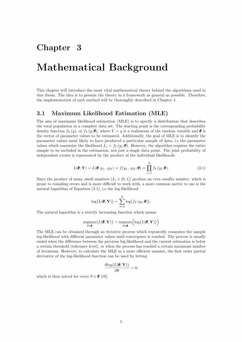
3.1 Maximum Likelihood Estimation (MLE)
The aim of maximum likelihood estimation (MLE) is to specify a distribution that describesthe total population in a complete data set. The starting point is the corresponding probabilitydensity function fY (y), or fY (y;θθθ), where Y = y is a realization of the random variable and θθθ isthe vector of parameter values to be estimated. Additionally, the goal of MLE is to identify theparameter values most likely to have produced a particular sample of data, i.e the parametervalues which maximize the likelihood Li = fY (yi;θθθ). However, the algorithm requires the entiresample to be included in the estimation, not just a single data point. The joint probability ofindependent events is represented by the product of the individual likelihoods
L(θθθ; Y) = L(θθθ; y1...yN ) = f(y1...yN ;θθθ) =
N∏i=1
fY (yi;θθθ). (3.1)
Since the product of many small numbers (Li ∈ [0, 1]) produce an even smaller number, which isprone to rounding errors and is more difficult to work with, a more common metric to use is thenatural logarithm of Equation (3.1), i.e the log-likelihood
log(L(θθθ; Y)
)=
N∑i=0
log(fY (yi;θθθ)
).
The natural logarithm is a strictly increasing function which means
argmaxθ∈θθθ
(L(θθθ; Y)
)= argmax
θ∈θθθ
(log(L(θθθ; Y)
))The MLE can be obtained through an iterative process which repeatedly computes the samplelog-likelihood with different parameter values until convergence is reached. The process is usuallyended when the difference between the previous log-likelihood and the current estimation is belowa certain threshold (tolerance level), or when the process has reached a certain maximum numberof iterations. However, to calculate the MLE in a more efficient manner, the first order partialderivative of the log-likelihood function can be used by letting
∂log(L(θθθ; Y)
)∂θ
= 0,
which is then solved for every θ ∈ θθθ [10].
5

3.2 Bayesian InferenceIn probability theory there are two fundamentally different approaches regarding the interpreta-tion of the set of parameters to be estimated. They consist of the Frequentist inference and theBayesian inference. In the Frequentist analysis approach the data is interpreted as a repeatablerandom sample, and the estimated parameters to be fixed, i.e f(Y;θθθ). However, in the Bayesianframework the data is assumed to be observed from a realized sample, and the parameters tobe estimated are referred to as random variables, i.e f(θθθ|Y = y). More specific, the Bayesianframework consist of three essential steps
1. specify prior distributions for the included parameters
2. assign a likelihood function to include the information held by the data regardingthe different parameter values, and
3. combine the prior distributions and the likelihood to form a posterior distributionthat describes the relative probability across a range of parameter values [10].
The prior distributions are used to incorporate additional information to the model that isnot explained by the data alone. The intuition of assigning a uniform prior is hence that noadditional information is available or used. Based on the data, the likelihood function givesinformation regarding the relative probability for different parameter values. Additionally, theprior information regarding the parameters and the information attained from the data is thenused to form the posterior distribution of the parameters given the data via Bayes’ theorem, seeEquation (3.2).
f(θθθ|Y) =f(Y|θθθ)f(θθθ)
f(Y)(3.2)
In Equation (3.2) the parameters of interest are given by θθθ, and Y is the sample data. Theprior distribution assigned to θθθ is given by f(θθθ), the likelihood (i.e the distribution of the dataconditional on the parameter) is given by f(Y|θθθ), and the marginal distribution of the data isgiven by f(Y). The posterior distribution (i.e the distribution of the parameter conditional onthe data) is then given by f(θθθ|Y). The denominator of Equation (3.2) is just a normalizingconstant used to ensure that the area under the distribution function integrates to one, in otherwords
Posterior =Likelihood · Prior
Normalizing constant.
The shape of the posterior distribution is not affected by this constant, which often is difficult tocalculate. Hence, a more common way to express the posterior distribution is to exclude thisconstant (see [10]) and write
Posterior ∝ Likelihood · Prior.
3.3 Expectation Conditional Maximization (ECM)The MLE is an attractive tool when managing data. However, since the MLE is based on thefirst derivative of the log-likelihood function for every observed event it becomes intractable whenworking with missing data. Hence, another approach for the maximum likelihood estimation isneeded. The expectation conditional maximization (ECM) algorithm is an updated version of theclassical expectation maximization (EM) method first introduced by Dempster et al. (1977) [6],and is an appealing solution to the missing data estimation problem. The ECM algorithmfunctions partially under the Bayesian assumptions and will through an iterative process in-clude the conditional probability distribution of the missing data and provide a correspondingmaximum-a-posteriori (MAP) estimate of the parameter vector θθθ, i.e the mode value from its
6

posterior distribution.
The EMC is a two-step iterative estimation process. The first step is the expectation step (E-step)and the second step is the conditional maximization step (CM-step). The E-step generates samplesof missing (or latent) data by taking expectations over complete-data conditional distributions.Thereafter, the CM-step involves individual complete-data maximum likelihood estimation of eachparameter, by conditionally keeping the other parameters fixed. The CM-step is what separatesthe original EM method from the ECM algorithm. In the EM approach the correspondingM-step is maximizing the likelihood function with respect to all parameters at the same time.Hence, even if the ECM method is more computer intensive in the sense of number of iterations,the overall rate of convergence may be improved. The objective of the ECM algorithm is tomaximize the observed-data likelihood by iteratively maximizing the complete-data likelihood [25].
Consider the complete-data Y = (Yobs,Ymiss), where Yobs refers to the observed-data andYmiss the missing-data. By using Bayes’ theorem, see Equation (3.2), the likelihood of thecomplete-data can be written as
fY (Y|θθθ) = fYobs,Ymiss(Yobs,Ymiss|θθθ) = fYmiss(Ymiss|θθθ,Yobs) · fYobs(Yobs|θθθ)
⇒ fYobs(Yobs|θθθ) =fYobs,Ymiss(Yobs,Ymiss|θθθ)fYmiss(Ymiss|θθθ,Yobs)
,
where fYmiss(Ymiss|θθθ,Yobs) is the conditional distribution of the missing data given the observeddata. The relation between the complete-data likelihood L(θθθ; Y) and the observed-data likelihoodL(θθθ; Yobs) is then given by
log(L(θθθ; Yobs)
)= log
(L(θθθ; Y)
)− log
(fYmiss(Ymiss|θθθ,Yobs)
). (3.3)
The E-step now yields taking the expectation of Equation (3.3) with respect to fYmiss(Ymiss|θθθ,Yobs),i.e
log(L(θθθ; Yobs)
)= Eθθθ0
[log(L(θθθ; Y)
)]− Eθθθ0
[log(fYmiss(Ymiss|θθθ,Yobs)
)], (3.4)
for any initial value θθθ0. Since the expectation is taken with respect to the missing data Ymiss,the left hand side is by definition deterministic and the expectation is omitted. A common ECMnotation for the expected log-likelihood (see [31]) is
Q(θθθ|θθθ0,Yobs) = Eθθθ0[log(L(θθθ; Y)
)]. (3.5)
The consecutive CM-step then maximizes Equation (3.5) by
Q(θθθ(m+1)
∣∣∣θθθ(m),Yobs
)= max
θθθ
[Q(θθθ∣∣∣θθθ(m),Yobs
)]. (3.6)
If θθθm =(θ
(1)(m), ..., θ
(N)(m)
)is the parameter estimate at iteration m, m = 0, ...,M , the ECM
sequentially maximize Equation (3.5) through the following scheme
7

Q(θ
(1)(m+1)
∣∣∣θ(1)(m), ..., θ
(k)(m), ..., θ
(N)(m),Yobs
)= max
θ(1)
[Q(θ(1)∣∣∣θ(1)
(m), ..., θ(k)(m), ..., θ
(N)(m),Yobs
)]...
Q(θ
(2)(m+1)
∣∣∣θ(1)(m+1), θ
(2)(m), ..., θ
(k)(m), ..., θ
(N)(m),Yobs
)= max
θ(2)
[Q(θ(2)∣∣∣θ(1)
(m+1), θ(2)(m)..., θ
(k)(m), ..., θ
(N)(m),Yobs
)]...
Q(θ
(N)(m+1)
∣∣∣θ(1)(m+1), ..., θ
(k)(m+1), ..., θ
(N−1)(m+1) , θ
(N)(m),Yobs
)= max
θ(N)
[Q(θ(N)
∣∣∣θ(1)(m+1), ..., θ
(k)(m+1), ..., θ
(N−1)(m+1) , θ
(N)(m),Yobs
)].
In other words, the ECM algorithm maximize Equation (3.5) by first maximizing with respect
to θ(1)(m) keeping all other parameters constant. The fundamental in the theory behind the
ECM algorithm is that the observed likelihood in Equation (3.4) is increased by maximizingQ(θθθ|θθθ0,Yobs) in each iteration. The following theorem and proof is referred to by Robert et al.in [31], but were first stated by Dempster et al. (1977) [6].
Theorem 3.3.1. The sequence(θ(m)
)defined by Equation (3.6) satisfies
L(θ(m+1)
∣∣∣Yobs
)≥ L
(θ(m)
∣∣∣Yobs
)with equality holding if and only if Q
(θ(m+1)
∣∣∣θ(m),Yobs
)= Q
(θ(m)
∣∣∣θ(m),Yobs
).
Proof. On successive iterations, it follows from the definition of θm+1 that
Q(θ(m+1)
∣∣∣θ(m),Yobs
)≥ Q
(θ(m)
∣∣∣θ(m),Yobs
).
Hence, if it can be showed that
Eθ(m)
[log
(fYmiss
(Ymiss
∣∣∣θ(m+1),Yobs
))]≤ Eθ(m)
[log
(fYmiss
(Ymiss
∣∣∣θ(m),Yobs
))], (3.7)
it will follow from Equation (3.4) that the value of the likelihood is increased at each iteration.By defining the Shannon entropy, first introduced by Shannon [36] in 1948, as
H(θ(m+1)
∣∣∣θ(m)
)= −Eθ(m)
[log
(fYmiss
(Ymiss
∣∣∣θ(m+1),Yobs
))]
= −∫
Ymiss
log
(fYmiss
(Ymiss
∣∣∣θ(m+1),Yobs
))· fYmiss
(Ymiss
∣∣∣θ(m),Yobs
)dYmiss,
and by using the Gibbs inequality2 [2]
2 For a continuous probability distribution F =∫fX(x)dx, and any other continuous probability distribution
Q =∫qX(x)dx, the Gibbs inequality states
−∫
log(fX(x)
)· fX(x)dx ≤ −
∫log(qX(x)
)· fX(x)dx,
with equality only if f = q.
8

−∫
Ymiss
log
(fYmiss
(Ymiss
∣∣∣θ(m),Yobs
))· fYmiss
(Ymiss
∣∣∣θ(m),Yobs
)dYmiss
≤
−∫
Ymiss
log
(fYmiss
(Ymiss
∣∣∣θ(m+1),Yobs
))· fYmiss
(Ymiss
∣∣∣θ(m),Yobs
)dYmiss
⇒
H(θ(m)
∣∣∣θ(m)
)≤ H
(θ(m+1)
∣∣∣θ(m)
),
the theorem is established.
However, Theorem 3.3.1 does not confirm that the sequence θ(m) converges to its correspondingMLE estimate. The following complementing theorem is given by Roberts et al. [31] to ensureconvergence to a stationary point, i.e either a local maximum or a saddle point.
Theorem 3.3.2. If the expected complete-data likelihood Q(θ|θ0,Yobs) is continuous in both θ
and θ0, then every limit point of an EM sequence θ(m) is a stationary point of L(θ|Yobs) and
L(θ(m)
∣∣∣Yobs
)converges monotonically to L
(θ∣∣∣Yobs
)for some stationary point θ.
Be aware that Theorem 3.3.2 only guarantees convergence to a stationary point and not a globalmaximum. This problem can be solved by running the ECM algorithm a number of times usingdifferent initial values [31].
In Appendix A a short example [28] of the derivation of the ECM updating formula for the oneparameter case can be found.
3.4 Regression AnalysisThe basic idea of the linear regression model is to build a set of regression equations to estimatethe conditional expectation of a set of random variables Y = (Y1, ..., Yn), see Equation (3.8).
yi =
k∑j=0
xi,jβj + ei, i = 1, ..., N. (3.8)
The predicted value yi is a realisation of the dependent random variable Yi whose value dependson the explanatory variables (covariates) xi,j . In contrast to the observed covariates, the residuals,ei, are random variables and are assumed to be independent between observations, and withconditional expected value and variance
E[ei|x] = 0 and E[e2i
∣∣∣x] = σ2,
where σ is typically unknown [22]. However, this representation of the residuals is under theassumption of homoskedasticity3. This is often an unverified assumption, and in many casesheteroskedasticity4 is a more appropriate premise [16].
To bring more power to the estimated regression model it is strongly recommended to constructa regression equation with high correlation between the explanatory variables and the dependentvariable, but with little to none correlation among the covariates themselves. Additionally, thepresence of multicollinearity5 can otherwise induce uncertainty regarding the inference to be
3 Homoskedasticity is when E[e2i
∣∣∣x] = σ2, i.e the residual variance does not depend on the observation.
4 Heteroskedasticity is when E[e2i
∣∣∣x] = σ2i , i.e the residual variance depends on the observation.
5 Multicollinearity arises when two or more covariates are perfectly correlated.
9

made about the model, even if the phenomenon in general does not reduce power or influencethe reliability of the model [22].
However, the first covariate, xi,0, is usually set to 1. This means that the first coefficient β0, calledthe intercept, in (3.8) acts as a constant term. Hence, in contrast to the other coefficients theintercept is somewhat hard to interpret since it does not indicate how much a specific covariatecontributes to the estimation of the dependent variable. However, the intercept is essential andis included to reduce bias by shifting the regression line, and therefore guaranteeing that theconditional expected value of the residual is E[ei|x] = 0 [15].
3.5 Copulas
The name copula is a Latin noun that means a ”link, tie, bond” [27]. In probability theory acopula is a function used to describe and model the relation between one-dimensional distributionfunctions, when the corresponding joint distribution is intractable. The name and theory behindcopulas (in the mathematical context) was first introduced by Sklar in 1959. Still, an informativeintroduction to copulas (which is some what easy to digest) can be found in Embrechts et al. [8],in Lindskog et al. [7] and in Embrechts [9]. More extensive literature concerning this subject ispresented by Nelsen [27] and by Dall’Aglio et al. [4]. However, the theorems and correspondingproofs behind the theory of copulas in this paper is stated as in McNeil et al. [24].
A copula is defined in McNeil et al. [24] as:
Definition 3.5.1. A d-dimensional copula is a distribution function on [0, 1]d with standarduniform marginal distributions. The notation C(u) = C(u1, ..., ud) is reserved for the multivariatedistribution functions that are copulas. Hence C is a mapping of the form C : [0, 1]d → [0, 1], i.e.a mapping of the unit hypercube into the unit interval. The following three properties must hold.
1. C(u1, ..., ud) is increasing in each component ui.
2. C(1, ..., 1, ui, 1, ..., 1) = ui for all i ∈ 1, ..., d, ui ∈ [0, 1].
3. For all (a1, ..., ad), (b1, ..., bd) ∈ [0, 1]d with ai ≤ bi, the following must apply
2∑i1=1
...
2∑id=1
(−1)i1+...+idC(u1i1 , ..., udid) ≥ 0, (3.9)
where uj1 = aj and uj2 = bj for all j ∈ 1, ..., d.
The first property is clearly required of any multivariate distribution function and the second prop-erty is the requirement of uniform marginal distributions. The third property is less obvious, butthe so-called rectangle inequality in Equation (3.9) ensures that if the random vector (U1, ..., Ud)
′
has distribution function C, then P (a1 ≤ U1 ≤ b1, ..., ad ≤ Ud ≤ bd) is non-negative. These threeproperties characterize a copula; if a function C fulfills them, then it is a copula.
Before stating the famous Sklar’s Theorem, which is of great importance in the the study ofmultivariate distribution functions, the operations of probability and quantile transformationtogether with the properties of generalized inverses must be introduced, see Proposition 3.5.1.The proof and the underlying theory to Proposition 3.5.1 can be found in [24].
Proposition 3.5.1. Let G be a distribution function and let G← denote its generalized inverse,i.e. the function G←(y) = inf{x : G(x) ≥ y}.
1. Quantile transformation. If U ∼ U(0, 1) has a standard uniform distribution,then P (G←(U) ≤ x) = G(x).
2. Probability transformation. If Y has distribution function G, where G is acontinuous univariate distribution function, then G(Y ) ∼ U(0, 1).
10
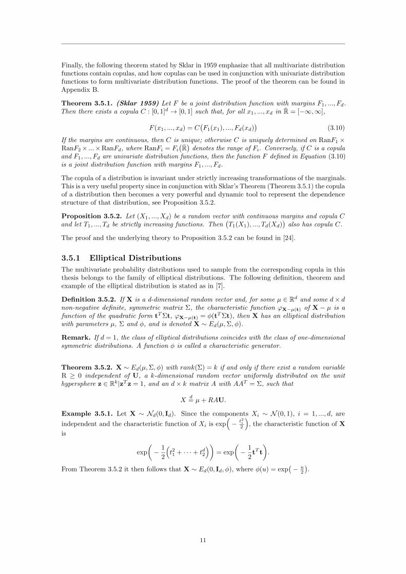
Finally, the following theorem stated by Sklar in 1959 emphasize that all multivariate distributionfunctions contain copulas, and how copulas can be used in conjunction with univariate distributionfunctions to form multivariate distribution functions. The proof of the theorem can be found inAppendix B.
Theorem 3.5.1. (Sklar 1959) Let F be a joint distribution function with margins F1, ..., Fd.Then there exists a copula C : [0, 1]d → [0, 1] such that, for all x1, ..., xd in R = [−∞,∞],
F (x1, ..., xd) = C(F1(x1), ..., Fd(xd)
)(3.10)
If the margins are continuous, then C is unique; otherwise C is uniquely determined on RanF1 ×RanF2× ...×RanFd, where RanFi = Fi
(R)
denotes the range of Fi. Conversely, if C is a copulaand F1, ..., Fd are univariate distribution functions, then the function F defined in Equation (3.10)is a joint distribution function with margins F1, ..., Fd.
The copula of a distribution is invariant under strictly increasing transformations of the marginals.This is a very useful property since in conjunction with Sklar’s Theorem (Theorem 3.5.1) the copulaof a distribution then becomes a very powerful and dynamic tool to represent the dependencestructure of that distribution, see Proposition 3.5.2.
Proposition 3.5.2. Let (X1, ..., Xd) be a random vector with continuous margins and copula Cand let T1, ..., Td be strictly increasing functions. Then
(T1(X1), ..., Td(Xd)
)also has copula C.
The proof and the underlying theory to Proposition 3.5.2 can be found in [24].
3.5.1 Elliptical Distributions
The multivariate probability distributions used to sample from the corresponding copula in thisthesis belongs to the family of elliptical distributions. The following definition, theorem andexample of the elliptical distribution is stated as in [7].
Definition 3.5.2. If X is a d-dimensional random vector and, for some µ ∈ Rd and some d× dnon-negative definite, symmetric matrix Σ, the characteristic function ϕX−µ(t) of X − µ is afunction of the quadratic form tTΣt, ϕX−µ(t) = φ(tTΣt), then X has an elliptical distributionwith parameters µ, Σ and φ, and is denoted X ∼ Ed(µ,Σ, φ).
Remark. If d = 1, the class of elliptical distributions coincides with the class of one-dimensionalsymmetric distributions. A function φ is called a characteristic generator.
Theorem 3.5.2. X ∼ Ed(µ,Σ, φ) with rank(Σ) = k if and only if there exist a random variableR ≥ 0 independent of U, a k-dimensional random vector uniformly distributed on the unithypersphere z ∈ Rk|zT z = 1, and an d× k matrix A with AAT = Σ, such that
Xd= µ+RAU.
Example 3.5.1. Let X ∼ Nd(0, Id). Since the components Xi ∼ N (0, 1), i = 1, ..., d, are
independent and the characteristic function of Xi is exp(− t2i
2
), the characteristic function of X
is
exp
(− 1
2
(t21 + · · ·+ td2
))= exp
(− 1
2tT t
).
From Theorem 3.5.2 it then follows that X ∼ Ed(0, Id, φ), where φ(u) = exp(− u
2
).
11

Chapter 4
Methodology
In this chapter the mathematical theory from Chapter 3 is implemented in three differentmethods for imputation of missing data. More information regarding the underlying data andthe corresponding results are presented in Chapter 5 where they are put in the context of thesolution of a real world problem.
4.1 Stochastic Regression ImputationStochastic regression is, as the name implies, an evolved version of the ordinary regression analysis.In resemblance with the expected value imputation, described in Chapter 2, ordinary regressionimputation also suffers from lost variability and is therefore likely to induce bias. Stochasticregression modelling effectively restores this variability in the data by adding a random variableto the regression equation
yi =
k∑j=0
xi,j βj + zi, i = 1, ..., N, (4.1)
where yi is the estimate of the predicted variable, xi,j is the known covariate, βj is the corres-ponding parameter estimate and zi is the added noise variable. The matrix representation ofEquation (4.1) is given by
Y = Xβββ + z, (4.2)
where
Y =
y1
...yN
, X =
1 x1,1 . . . x1,j . . . x1,k
......
. . ....
. . ....
1 xN,1 . . . xN,j . . . xN,k
, βββ =
β0
...
βk
, and z =
z1
...zN
.The coefficients in Equation (4.2) are estimated using the ECM algorithm, which is introducedin Chapter 3. In contrast to the widespread use of the Ordinary Least Squares (OLS) method,the ECM algorithm make use of information attained from the missing data in the estimationprocess.
Two different assumptions regarding the distribution of the data is used during the estimation andimputation phases. First a normality assumption is applied by regarding the data as realisationsfrom a normal distribution as in Enders (2010) [10]. However, since the data is known to beheavy tailed, this procedure is further developed by also implementing the assumption that thedata belongs to a Student’s t-distribution (t-distribution).
The parameters are estimated using a full Bayesian implementation of the ECM algorithm. Inother words, the posterior distribution is derived by specifying prior distributions for the modelparameters and assigning a likelihood function for the data as in Section 3.2. However, to makethe derivation easier to follow the likelihood function is first assigned to the data, and then theprior distributions are specified for each parameter.
12

4.1.1 The Likelihood Function
Consider the complete d-variate data vector yi. Next, the assumption that the complete databelongs to a multivariate t-distribution
yi|ν,βββ,ΨΨΨ ∼ t(ν,Xi,0:kβββ,ΨΨΨ) (4.3)
fyi(yi|ν,βββ,ΨΨΨ) ∝ |ΨΨΨ| 12(
1 +1
ν(yi −Xi,0:kβββ)′ΨΨΨ(yi −Xi,0:kβββ)
)− ν+d2
,
with shape matrix6 ΨΨΨ, is applied by using a mixture of normal distributions together with aprior distribution of an auxiliary weight parameter wi. More specific, the corresponding priordistribution of the weight vector and the normal mixture assigned to the observations are givenby
wi|ν ∼ Gamma(ν
2,ν
2
)=
(ν2
)( ν2 )
Γ(ν2
) (wi)ν2−1e−
ν2wi (4.4)
fwi(wi|ν) ∝ (wi)ν2−1e−
ν2wi
and
yi|ν,βββ,ΨΨΨ, wi ∼ N(Xi,0:kβββ, (wiΨΨΨ)−1
)=|wiΨΨΨ|
12
√2π
e−wi2 (yi−Xi,0:kβββ)′ΨΨΨ(yi−Xi,0:kβββ)
fyi(yi|ν,βββ,ΨΨΨ, wi) ∝ |wiΨΨΨ|12 e−
wi2 (yi−Xi,0:kβββ)′ΨΨΨ(yi−Xi,0:kβββ),
where | · | is the determinant and Γ(·) is the Gamma function. If the N × d vector Y =[y1, ...,yi, ...,yN
]′of observations is assumed to be conditionally independent, the total likeli-
hood is
fY(Y|ν,βββ,ΨΨΨ,ωωω) =
N∏i=1
fyi(yi|ν,βββ,ΨΨΨ, wi)
∝ |ΨΨΨ|N2 ·N∏i=1
(wi)d2 · e− 1
2
∑Ni=1 wi(yi−Xi,0:kβββ)′ΨΨΨ(yi−Xi,0:kβββ).
In consistency with Section 3.2 the sign ∝ means ”proportional to” and indicates that somenormalizing constants have been omitted [30].
4.1.2 The Prior Distribution
The parameter βββ is assigned a uniform prior distribution (see [23]) given by
βββ ∝ constant.
The specified joint prior distribution for the parameter ΨΨΨ is given by an uninformative version ofthe inverse Wishart distribution with density
ΨΨΨ ∼ |ΛΛΛ| ν22ν·d2 Γd
(ν2
) |ΨΨΨ|− ν+d+12 e−
12 tr(ΛΛΛΨΨΨ−1
),
ΨΨΨ ∝ |ΨΨΨ|−ν+d+1
2 e−12 tr(ΛΛΛΨΨΨ−1
), (4.5)
6 The relation between the MAP estimate of the shape matrix and the covariance matrix is for the normal
distribution given by Σ = ΨΨΨ−1
, and for the t-distribution Σ = νν−2
ΨΨΨ−1
, (ν > 2).
13

where Γd(ν2
)is the multivariate gamma function and tr(·) is the trace 7. In this case the word
uninformative means that no initial assumptions regarding the distribution of ΨΨΨ are applied. Morespecific, setting ν = 0 and Λ = 0 in Equation (4.5) is akin to say that no additional informationregarding the distribution is used [10]. This means that the improper8 prior distribution ofΨΨΨ (see [30]) is proportional to
fΨΨΨ(ΨΨΨ) ∝ |ΨΨΨ|−d+12 .
4.1.3 The Posterior Distribution
By using Bayes’ theorem (see Equation (3.2)) and assuming that ωωω,βββ,ΨΨΨ are a-priori independentfinally gives the posterior distribution
fν,βββ,ΨΨΨ,ωωω(ν,βββ,ΨΨΨ,ωωω|Y) ∝ fY(Y|ν,βββ,ΨΨΨ,ωωω) · fβββ(βββ) · fΨΨΨ(ΨΨΨ) · fωωω(ωωω|ν)
∝ |ΨΨΨ|N−d−1
2
N∏i=1
(wi)d+ν2 −1e−
12
∑Ni=1 wi
((yi−Xi,0:kβββ)′ΨΨΨ(yi−Xi,0:kβββ)+ν
)(4.6)
Given the full posterior distribution in Equation (4.6), the posterior conditional distribution foreach parameter can be derived.
The posterior distribution of the weights, conditional on (Y, ν,βββ,ΨΨΨ), is attained by omittingeverything in Equation (4.6) not depending on ωωω, i.e
fωωω(ωωω|Y, ν,βββ,ΨΨΨ) ∝N∏i=1
(wi)d+ν2 −1 · e−
12
∑Ni=1 wi
((yi−Xi,0:kβββ)′ΨΨΨ(yi−Xi,0:kβββ)+ν
). (4.7)
By inspection, the Equation (4.7) is proportional to the closed form expression of the gammadistribution (see Equation (4.4)), hence
wi|yi, ν,βββ,ΨΨΨ ∼ Gamma(d+ ν
2,
(yi −Xi,0:kβββ)′ΨΨΨ(yi −Xi,0:kβββ) + ν
2
)fωωω(ωωω|Y, ν,βββ,ΨΨΨ) =
N∏i=1
f(wi|yi, ν,βββ,ΨΨΨ).
The corresponding conditional expectation of the weights is then given by
E[wi∣∣yi, ν,βββ,ΨΨΨ] =
d+ ν
(yi −Xi,0:kβββ)′ΨΨΨ(yi −Xi,0:kβββ) + ν. (4.8)
Continuing with the posterior conditional distribution of the shape matrix ΨΨΨ, and comparingEquation (4.6) with the Wishart distribution
|ΨΨΨ| ν−d−12 e−
12 tr(ΛΛΛ−1ΨΨΨ
)2ν·d2 |ΛΛΛ| ν2 Γd
(ν2
) ,
gives
7 The trace of an n× n square matrix A is defined to be the sum of the elements on the main diagonal of A, i.etr(A) = a11 + a22 + ...+ ann =
∑ni=1 aii
8 Improper in the sense that it does not integrate to 1.
14

ΨΨΨ|Y, ν,βββ,ωωω ∼Wishart(Λ−1, N)
fΨΨΨ(ΨΨΨ|Y, ν,βββ,ωωω) ∝ |ΨΨΨ|N−d−1
2 · e− 12 tr(ΨΨΨΛ),
where
N∑i=1
wi(yi −Xi,0:kβββ)ΨΨΨ(yi −Xi,0:kβββ)′ = tr(ΨΨΨΛΛΛ)
and
Λ =
N∑i=1
wi(yi −Xi:kβββ)(yi −Xi,0:kβββ)′.
The MAP estimate of the posterior conditional distribution of the shape matrix ΨΨΨ is then givenby
mode(ΨΨΨ|Y, ν,βββ,ωωω) = (N − d− 1) ·Λ−1, (4.9)
for N > d − 1. Finally, by examining Equation (4.6) it can be seen that the posterior condi-tional distribution of the coefficient vector βββ is normal (see [30]), and the MAP estimate is given by
mode(βββ|Y, ν,ΨΨΨ,ωωω) =
(N∑i=1
wi(Xi,0:k)′ΨΨΨXi,0:k
)−1 N∑i=1
wi(Xi,0:k)′ΨΨΨyi. (4.10)
4.1.4 Imputation Procedure
The iterative ECM method is used to attain the MAP estimates of the corresponding posteriorconditional distributions. However, until now the estimation of the degrees of freedom parameter,ν, has not been considered. In comparison with the other parameters the estimation of thedegrees of freedom parameter, ν, is a bit more tedious.
Estimation of the Degrees of Freedom Parameter, ν
Given the marginal distribution of the observed weights (see Equation (4.4)) the correspondinglog-likelihood of ν, ignoring constants, is given by
LGamma(ν|ωωω) ∝ −N · ln(
Γ
(ν
2
))+N · ν
2· ln(ν
2
)+ν
2·N∑i=1
(ln(wi)− wi
). (4.11)
However, the representation in Equation (4.11) is assuming that the weights, wi, are known.Hence, when the weights are unknown the last term in Equation (4.11) is replaced by itsconditional expectation, i.e by
E
[N∑i=1
(ln(wi)− wi
)|Y, ν,βββ,ΨΨΨ
]= φ
(d+ ν
2
)− ln
(d+ ν
2
)
+
N∑i=1
(ln(E[wi∣∣Y, ν,βββ,ΨΨΨ
])− E
[wi∣∣Y, ν,βββ,ΨΨΨ
]),
where φ(·) is the digamma function9 and E[wi∣∣Y, ν,βββ,ΨΨΨ
]is given by Equation (4.8).
9 The digamma function is defined as φ(x) =dln(Γ(x)
)dx
.
15

The degrees of freedom parameter is then attained by maximizing Equation (4.11) with respectto ν. In other words, at iteration (m+ 1) of the ECM algorithm the value of ν is obtained byfinding the solution to the following equation
0 =− φ(ν
2
)+ ln
(ν
2
)+ 1 + φ
(d+ ν(m)
2
)− ln
(d+ ν(m)
2
)
+1
N
N∑i=1
(ln(w
(m)i
)− w(m)
i
). (4.12)
The solution to Equation (4.12) can be found by a one-dimensional search using a half intervalmethod. In this thesis Equation (4.12) is solved using the MATLAB function Bisection [3], seealso [1] for more information. Additionally, for a more thorough derivation of Equation (4.12)see [23].
Treating Missing Values
Until now, the missing data Ymiss in Y =(Yobs,Ymiss
)has not been covered in the estimation
process. In the parameter estimation process the missing data is temporary filled in using theconditional expectation
E[Ymiss|Yobs = yobs] = Xβββ −ΣΣΣYobs,YmissΣΣΣ−1Yobs,Ymiss
(yobs −Xβββ),
and then the conditional covariance of Ymiss|Yobs = yobs is updated via
ΣΣΣYmiss|Yobs=yobs = ΣΣΣYmiss−ΣΣΣYobs,Ymiss
ΣΣΣ−1Yobs,Yobs
ΣΣΣYmiss,Yobs.
Implementing the ECM Algorithm
Consider a N ×d vector y = (yobs,ymiss), where N = (Nobs, Nmiss) is the number of observationand missing values in y. The ECM algorithm is then used to obtain the MAP estimates of eachparameter, see Algorithm (1). The E-step corresponds to Equation (4.8) and the CM-steps toEquations (4.9), (4.10) and (4.12).
16

Algorithm 1: The ECM Algorithm
1: Initialize ymiss ← 0, ΨΨΨ(0)obs ← I, ΨΨΨ(0) =
(ΨΨΨ
(0)obs, ΨΨΨ
(0)miss
), ωωω(0) ← 1 and ν(0) ← 4.
2: while∣∣βββ(m+1) − βββ(m)
∣∣ ≥ tolerance do
3: βββ(m+1) ←(∑N
i=1 w(m)i yi(Xi,0:k)
′ΨΨΨ(m)Xi,0:k
)−1∑Ni=1 w
(m)i (Xi,0:k)ΨΨΨ(m)yi
4: Λ(m+1) ←∑Ni=1 w
(m)i
(yi −Xi,0:kβββ
(m+1))(
yi −Xi,0:kβββ(m+1)
)′5: ΨΨΨ(m+1) ← (N − d− 1)
(Λ(m+1)
)−1
6: Solve for ν:
0 =− φ(ν
2
)+ ln
(ν
2
)+ 1 + φ
(d+ ν(m)
2
)
− ln
(d+ ν(m)
2
)+
1
N
N∑i=1
[ln(w
(m)i
)− w(m)
i
]
7: Set ν(m+1) = ν8: for i = 1 to N do9: w
(m+1)i ← d+ν(m+1)
ν(m+1)+(yi−Xi,0:kβββ(m+1))′ΨΨΨ(m+1)(yi−Xi,0:kβββ(m+1))
10: end for11: Treating missing values12: for i = 1 to Nmiss do
13: y(m+1)miss,i = Xi,0:kβββ
(m+1) −(ΨΨΨ
(m+1)obs,miss
)−1
ΨΨΨ(m+1)obs,obs
(yobs,i −Xi,0:kβββ
(m+1))
14: end for
15:
(ΨΨΨ
(m+1)miss|obs
)−1
←(ΨΨΨ
(m+1)miss
)−1
−(ΨΨΨ
(m+1)obs,miss
)−1
ΨΨΨ(m+1)obs,obs
(ΨΨΨ
(m+1)miss,obs
)−1
16: Set ΨΨΨ(m+1)miss ←ΨΨΨ
(m+1)miss|obs
17: Set ΨΨΨ(m+1) ←(ΨΨΨ
(m+1)obs ,ΨΨΨ
(m+1)miss
)18: end while
The MAP estimate for the normal regression, i.e letting ν →∞, is obtained by neglecting theweight update in lines 8-10. The ECM routine described above is implemented through anupdated version of the MATLAB function, mvsregress [30]. In the original version of mvsregressthe degrees of freedom, ν, is assumed to be known, and the function hence exclude the estimationin line 6 in Algorithm 1.
The estimated coefficients in Equation (4.1) and the degrees of freedom parameter, with differentamount of missing data (NaN), can be found in Table 4.1.
Normal distributionNaN β0 β1 β2 ν
0 0.0205 0.5744 0.5394 ∞3 0.0217 0.5741 0.5401 ∞10 0.0197 0.5734 0.5412 ∞25 0.0213 0.5723 0.5401 ∞50 0.0337 0.5563 0.5501 ∞100 0.0088 0.5426 0.5598 ∞150 0.0171 0.5370 0.5579 ∞250 0.0193 0.5342 0.5851 ∞
Student’s t-distributionNaN β0 β1 β2 ν
0 0.0153 0.5949 0.5058 2.89473 0.0164 0.5944 0.5068 2.913510 0.0140 0.5933 0.5088 2.932825 0.0135 0.5917 0.5074 2.970550 0.0162 0.5813 0.5173 3.3667100 0.0106 0.5724 0.5253 5.0469150 0.0127 0.5585 0.5394 6.2348250 0.0191 0.5494 0.5636 9.3356
Table 4.1: Estimated parameter values for the normal distribution assumption and the Student’st-distribution with different amount of missing data (NaN).
17
The predicted values are now computed using Equation (4.1) together with the parameterestimates from Table 4.1. The random noise variable zi is then added to every output to restorevariability to the imputed data. In the first model the noise term is assumed to have a normaldistribution with zero mean and a corresponding residual variance. In the model where the datais assumed to be heavy tailed the noise is generated by the t-distribution with zero mean andcorresponding residual variance and degree of freedom, i.e
zi ∼ N(0,ΨΨΨ−1
)zi ∼ t
(ν, 0,
ν
ν − 2ΨΨΨ−1
).
18

4.2 Multiple Imputation (MI)
Multiple imputation (MI) is an alternative to maximum likelihood estimation (MLE) and is theother method currently regarded as a state-of-the-art missing data technique [10]. The MI methodtends to produce similar analysis results as the MLE approach if the imputation model containsthe same variables as the subsequent analysis model. However, in the case when additionalvariables are used that are not included in the subsequent analysis the two approaches mayprovide different estimates, standard errors, or both. However, the main difference between themethods is that the analysis from the MI approach does not depend solely on one imputed set ofmissing values but of several augmented chains. For more information regarding the advantagesand disadvantages of the two methods please see [10]. The imputation approach outlined inthis section functions under the same assumption as in Section 4.1, i.e. that the data is missingat random (MAR). In line with Section 4.1 both a normal distribution and a t-distribution isassigned to the data. To attain the corresponding t-distribution, the approach used in Section 4.1,is also applied here.
MI is actually a broad term and include a variety of underlying imputation techniques, eachsuperior depending on the current missing data pattern and mechanism assumption. A multipleimputation analysis consists of three distinct steps common to all multiple imputation procedures:
• The imputation phase
• The analysis phase
• The pooling phase
In the imputation phase the underlying algorithm is used to estimate a multiple set of predictedvalues for each missing data point. In other words, a multiple set of parallel series are generatedfor each set of missing data. The underlying MI procedure used in this thesis is an iterative versionof the stochastic regression imputation technique from Section 4.1. However, the mathematicalprinciple behind the update of the parameter estimates rely heavily on Bayesian methodology.The goal of the analysis phase is, as its name implies, to individually analyze the filled-indata sets and estimate the corresponding parameters. With exception of the initial step, thisamounts to sequentially applying the same statistical procedures as if the data had been complete.Additionally, the analysis phase should hence produce a parameter estimate for each imputedparallel set of values from the imputation phase. The purpose of the final step, the pooling phase,is to estimate a single set of results by combining all the estimated parameters.
4.2.1 The Imputation Phase
The imputation phase is a data augmentation algorithm consisting of a two-step procedure, theactual imputation step (I-step) and the posterior step (P-step). The I-step uses the stochasticregression imputation technique from Section 4.1 to fill-in the set of missing values. More specific,the I-step uses an estimate of the mean vector and covariance matrix to construct a set ofregression equations to predict the missing values using the observed covariates.
The objective of the imputation phase is to generate a large number κ of complete data sets oflength N = Nobs +Nmiss, each of which contains augmented chains of length Nmiss of uniqueestimates of the missing values, see Table 4.2. To be able to attain these unique imputations, newestimates of the regression coefficients are required for each I-step. The purpose of the P-step istherefore to draw new candidates of the mean vector and covariance matrix from the respectiveposterior distribution. The imputation step is hence an iterative process which alternates betweenthe I-step and the P-step.
19

Y ∗κ,1 . . . Y ∗κ,Nobs Y ∗κ,Nobs+1 . . . Y ∗κ,Nobs+NmissY ∗κ−1,1 . . . Y ∗κ−1,Nobs
Y ∗κ−1,Nobs+1 . . . Y ∗κ−1,Nobs+Nmiss...
......
......
...Y ∗2,1 . . . Y ∗2,Nobs Y ∗2,Nobs+1 . . . Y ∗2,Nobs+NmissY ∗1,1 . . . Y ∗1,Nobs Y ∗1,Nobs+1 . . . Y ∗1,Nobs+Nmiss
Table 4.2: An overview of the κ number of complete data sets of length N = Nobs + Nmiss, each ofwhich contains augmented chains of length Nmiss of unique estimates of the missing values.
The I-Step
As described above, the purpose of the I-step is to construct a set of regression equations froman estimate of the mean vector and the covariance matrix. Since the procedure is an iterativeprocess alternating between the I-step and the P-step, the first iteration requires an initialestimate of the mean vector and the covariance matrix. Typically, a good starting point is touse the estimated parameters from the ECM algorithm used in Section 4.1. From these initialparameters estimates a first set of missing values are predicted from the observed covariates byusing stochastic regression imputation. In other words, the initial phase of the I-step produces afirst set of complete data, which the rest of the analysis is based upon.
Since the data is assigned a mixture of normal distributions together with an auxiliary weightvariable, wi, the corresponding unbiased10 Monte Carlo integration estimate of the expectedvalue and covariance of the complete data is given by
µY =1
N
N∑i=1
wiyi (4.13)
and
ˆCov(Y,Xj) =1
N − 1
N∑i=1
wi(yi − µY)(xi,j − µXj). (4.14)
The value of the auxiliary weight parameter wi is attained together with the initial parameterestimates using the ECM algorithm. Note that under the normal assumption the weight wi = 1,which is consistent with Section 4.1.
Given the estimated regression equation
Y = Xβββ + z,
where
Y =
y1
...yN
, X =
1 x1,1 . . . x1,j . . . x1,k
......
. . ....
. . ....
1 xN,1 . . . xN,j . . . xN,k
=[1 X1 . . . Xk . . . Xk
],
βββ =
β0
...
βk
, and z =
z1
...zN
,10 Unbiased in the sense that µ(·) = 1
N
∑Ni=1(·)→ E[·] as N →∞.
20
then the corresponding mean vector and covariance matrix is
µµµ =
µY
µX1
...µXk
, ΣΣΣ =
ˆCov(Y,Y) ˆCov(Y,X1) . . . ˆCov(Y,Xk)ˆCov(X1,Y) ˆCov(X1,X1) . . . ˆCov(X1,Xk)
......
. . ....
ˆCov(Xk,Y) ˆCov(Xk,X1) . . . ˆCov(Xk,Xk)
.
By using Equation (4.13) and (4.14) the regression coefficients are calculated by solving thefollowing set of equations
ˆCov(Y,Xi) =
k∑j=1
βj · ˆCov(Xj ,Xi).
and
β0 = µY − µµµX1:kβββ1:k,
or by using the subvector and submatrix of the mean vector and covariance matrix
βββ1:k =
ˆCov(X1,X1) . . . ˆCov(X1,Xk)
.... . .
...ˆCov(Xk,X1) . . . ˆCov(Xk,Xk)
−1
ˆCov(Y,X1)...
ˆCov(Y,Xk)
and
β0 = µY − µµµX1:kβββ1:k.
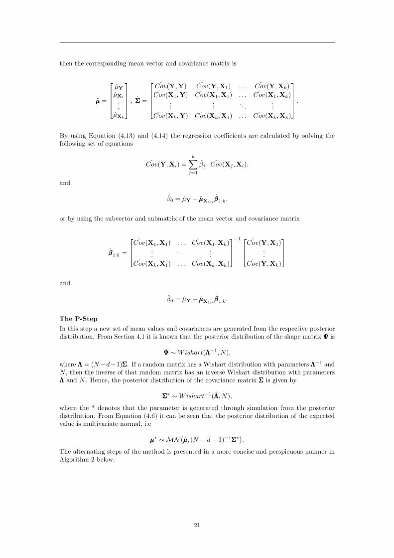
The P-Step
In this step a new set of mean values and covariances are generated from the respective posteriordistribution. From Section 4.1 it is known that the posterior distribution of the shape matrix ΨΨΨ is
ΨΨΨ ∼Wishart(ΛΛΛ−1, N),
where ΛΛΛ = (N−d−1)ΣΣΣ. If a random matrix has a Wishart distribution with parameters ΛΛΛ−1 andN , then the inverse of that random matrix has an inverse Wishart distribution with parametersΛΛΛ and N . Hence, the posterior distribution of the covariance matrix ΣΣΣ is given by
ΣΣΣ∗ ∼Wishart−1(ΛΛΛ, N),
where the * denotes that the parameter is generated through simulation from the posteriordistribution. From Equation (4.6) it can be seen that the posterior distribution of the expectedvalue is multivariate normal, i.e
µµµ∗ ∼MN(µµµ, (N − d− 1)−1ΣΣΣ∗
).
The alternating steps of the method is presented in a more concise and perspicuous manner inAlgorithm 2 below.
21

Algorithm 2: The Data Augmentation Algorithm of Multiple Imputation
1: Initialize βββ(0),w and ν via Algorithm 1.
2: Estimate Y = Xβββ(0)
3: ΨΨΨ(t) ← (N − d− 1)
(∑Ni=1 wi
(yi −Xi,0:kβββ
(t))(
yi −Xi,0:kβββ(t))′)−1
4: Draw z∗ ∼ N
(0,
(ΨΨΨ
(0))−1
)or z∗ ∼ t
(ν, 0, ν
ν−2
(ΨΨΨ
(0))−1
)5: Set Y(0) = Xβββ
(0)+ z∗
6: Estimate µµµ and ΣΣΣ7: for t = 1 to T do8: Set ΛΛΛ = (N − d− 1)ΣΣΣ
9: Draw ΣΣΣ∗(t) ∼Wishart−1(ΛΛΛ, N)10: Draw µµµ∗(t) ∼MN
(µµµ, (N − d− 1)−1ΣΣΣ∗(t)
)11: Compute βββ
(t)
1:k using ΣΣΣ∗(t)
12: Compute β(t)0 using µµµ∗(t)
13: Estimate Y = Xβββ(t)
14: ΨΨΨ(t) ← (N − d− 1)
(∑Ni=1 wi
(yi −Xi,0:kβββ
(t))(
yi −Xi,0:kβββ(t))′)−1
15: Draw z∗ ∼ N
(0,
(ΨΨΨ
(t))−1
)or z∗ ∼ t
(ν, 0, ν
ν−2
(ΨΨΨ
(t))−1
)16: Set Y(t) = Xβββ
(t)+ z∗
17: Estimate µµµ and ΣΣΣ18: end for
Initial I-Step
P-Step
I-Step
Convergence
The data augmentation algorithm used in the imputation phase belongs to a family of MarkovChain Monte Carlo (MCMC) procedures. The objective of a MCMC algorithm is to generaterandom draws from a distribution. By iteratively alternating between the I-step and the P-step,and sequentially generating new samples, a so-called data augmentation chain is created:
Y∗1 , θθθ∗1,Y
∗2 , θθθ∗2,Y
∗3 , θθθ∗3, . . . ,Y
∗t , θθθ∗t , . . . ,Y
∗T , θθθ∗T ,
where Y∗t represents the imputed values at I-step t, and θθθ∗t contains the generated parametervalues at P-step t. Note that the length of the total number of generated complete sets, T , ismuch greater than the final number of unique independent complete sets, κ.
In contrast to maximum likelihood based algorithms which reach convergence when the parameterestimates do not change over consecutive iterations, data augmentation converges when thedistributions become stationary11. The complexity of this definition is due to the fact that eachstep in the data augmentation chain is dependent on the former step. Hence, even if the dataaugmentation chain appears to be sequentially increased by random samples, the dependencebetween each I-step and P-step induces a correlation between the simulated parameters fromconsecutive P-steps. Additionally, analyzing data sets from consecutive I-steps inherit the sameproblem and is therefore also inappropriate. Consequently, to be able to generate a multipleof independent copies of the missing data it is essential to ensure when the data augmentation
11 Stationary in the sense that the expected value and variance do not change over time, i.e there is no visibletrend present.
22

chain has reached stationarity.
Monitoring the evolution of the chain over a large number of cycles is one way to accomplish this.In Figure 4.1-4.4 the first 200 iterations of the data augmentation chain of the expected valuesand the elements of the covariance matrix can be seen for the case with the greatest amount ofmissing values (in this case NaN=250). The horizontal line represents the corresponding mean ofthe total chain of T = 10, 000 iterations.
0 100 200
µY
-0.3
-0.25
-0.2
-0.15
-0.1
-0.05
0
0.05
0.1
0.15
0 100 200
µX
1
-0.5
-0.4
-0.3
-0.2
-0.1
0
0.1
0.2
Normal distribution
0 100 200
µX
2
-0.2
-0.15
-0.1
-0.05
0
0.05
0.1
0.15
Figure 4.1: The evolution of the data augmentation chain for the first 200 sampled expected valuesunder the normal assumption.
0 50 100 150 200
σ2 Y
6
6.5
7
7.5
8
0 50 100 150 200
σ2 X
1
9
10
11
12
Normal distribution
0 50 100 150 200
σ2 X
2
3
3.2
3.4
3.6
3.8
4
0 50 100 150 200
σY,X
1
6.5
7
7.5
8
8.5
9
0 50 100 150 200
σY,X
2
3.5
4
4.5
5
0 50 100 150 200
σX
1,X
2
3
3.5
4
4.5
Figure 4.2: The evolution of the data augmentation chain for the first 200 sampled elements of thecovariance matrix under the normal assumption.
23
0 100 200
µY
-0.4
-0.3
-0.2
-0.1
0
0.1
0.2
0 100 200
µX
1
-0.5
-0.4
-0.3
-0.2
-0.1
0
0.1
0.2
Students t-distribution
0 100 200
µX
2
-0.15
-0.1
-0.05
0
0.05
0.1
0.15
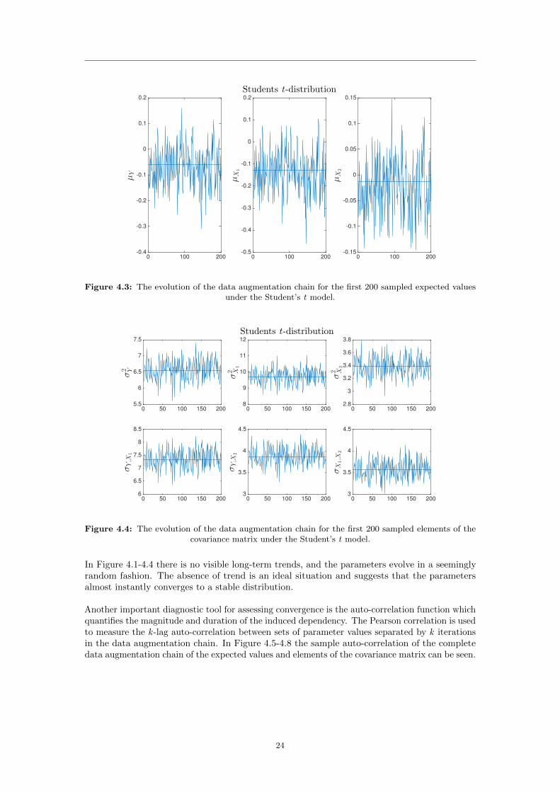
Figure 4.3: The evolution of the data augmentation chain for the first 200 sampled expected valuesunder the Student’s t model.
0 50 100 150 200
σ2 Y
5.5
6
6.5
7
7.5
0 50 100 150 200
σ2 X
1
8
9
10
11
12
Students t-distribution
0 50 100 150 200
σ2 X
2
2.8
3
3.2
3.4
3.6
3.8
0 50 100 150 200
σY,X
1
6
6.5
7
7.5
8
8.5
0 50 100 150 200
σY,X
2
3
3.5
4
4.5
0 50 100 150 200
σX
1,X
2
3
3.5
4
4.5
Figure 4.4: The evolution of the data augmentation chain for the first 200 sampled elements of thecovariance matrix under the Student’s t model.
In Figure 4.1-4.4 there is no visible long-term trends, and the parameters evolve in a seeminglyrandom fashion. The absence of trend is an ideal situation and suggests that the parametersalmost instantly converges to a stable distribution.
Another important diagnostic tool for assessing convergence is the auto-correlation function whichquantifies the magnitude and duration of the induced dependency. The Pearson correlation is usedto measure the k -lag auto-correlation between sets of parameter values separated by k iterationsin the data augmentation chain. In Figure 4.5-4.8 the sample auto-correlation of the completedata augmentation chain of the expected values and elements of the covariance matrix can be seen.
24
lag0 5 10 15 20
Sample
Autocorrelation
-0.2
0
0.2
0.4
0.6
0.8
1
µY
lag0 5 10 15 20
-0.2
0
0.2
0.4
0.6
0.8
1
µX1
lag0 5 10 15 20
-0.2
0
0.2
0.4
0.6
0.8
1
µX2
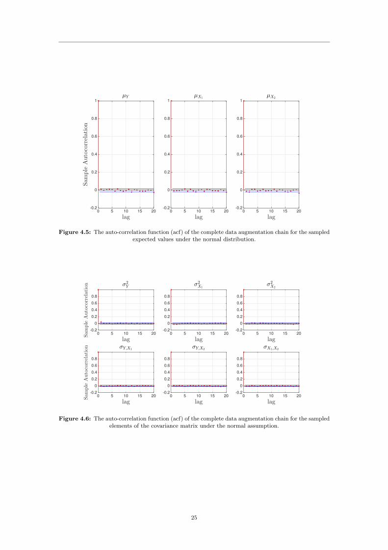
Figure 4.5: The auto-correlation function (acf) of the complete data augmentation chain for the sampledexpected values under the normal distribution.
lag0 5 10 15 20
Sample
Autocorrelation
-0.2
0
0.2
0.4
0.6
0.8
σ2Y
lag0 5 10 15 20
-0.2
0
0.2
0.4
0.6
0.8
σ2X1
lag0 5 10 15 20
-0.2
0
0.2
0.4
0.6
0.8
σ2X2
lag0 5 10 15 20
Sample
Autocorrelation
-0.2
0
0.2
0.4
0.6
0.8
σY,X1
lag0 5 10 15 20
-0.2
0
0.2
0.4
0.6
0.8
σY,X2
lag0 5 10 15 20
-0.2
0
0.2
0.4
0.6
0.8
σX1,X2
Figure 4.6: The auto-correlation function (acf) of the complete data augmentation chain for the sampledelements of the covariance matrix under the normal assumption.
25

lag0 5 10 15 20
Sample
Autocorrelation
-0.2
0
0.2
0.4
0.6
0.8
1
µY
lag0 5 10 15 20
-0.2
0
0.2
0.4
0.6
0.8
1
µX1
lag0 5 10 15 20
-0.2
0
0.2
0.4
0.6
0.8
1
µX2
Figure 4.7: The auto-correlation function (acf) of the complete data augmentation chain for the sampledexpected values under the Student’s t model.
lag0 5 10 15 20
Sample
Autocorrelation
-0.2
0
0.2
0.4
0.6
0.8
σ2Y
lag0 5 10 15 20
-0.2
0
0.2
0.4
0.6
0.8
σ2X1
lag0 5 10 15 20
-0.2
0
0.2
0.4
0.6
0.8
σ2X2
lag0 5 10 15 20
Sample
Autocorrelation
-0.2
0
0.2
0.4
0.6
0.8
σY,X1
lag0 5 10 15 20
-0.2
0
0.2
0.4
0.6
0.8
σY,X2
lag0 5 10 15 20
-0.2
0
0.2
0.4
0.6
0.8
σX1,X2
Figure 4.8: The auto-correlation function (acf) of the complete data augmentation chain for the sampledelements of the covariance matrix under the Student’s t model.
In Figure 4.5-4.8 the auto-correlation plots of the different parameters confirm the behavior inFigure 4.1-4.4. The auto-correlation drops to within sampling error of zero almost immediately.This suggests that the distribution of the parameters becomes stable after a very small numberof iterations.
26

Final Set of Imputations
As stated earlier, the main goal of the imputation phase is to generate a large number κ ofcomplete data sets, each of which contains unique estimates of the missing values. After analyzingthe complete data augmentation chains there are two approaches for attaining the final setof independent imputations, κ, namely by sequential and parallel sampling. Sequential dataaugmentation chains refers to saving and analysing the data sets at regular intervals, e.g. every20th I-step. Parallel data augmentation chains are generated by sampling several chains and saveand analyse the imputed data at the final I-step. In this thesis the final set of imputations aregenerated by using sequential sampling. To be certain that the data augmentation chain hasreached stationarity the generated samples are saved and analyzed every 100th I-step. Hence, atotal of T = 10, 000 iterations are required to attain κ = 100 imputed samples for each missingvalue.
4.2.2 The Analysis Phase
In the analysis phase the κ data sets are analyzed using the same procedure as if the datahad been complete. This phase is in a way integrated in Algorithm 2, and the mean vectorand covariance matrix of the corresponding κ final complete data sets are saved and analyzed.The regression coefficients are then computed through these κ sets of independently sampledparameters and are combined to a single estimate in the subsequent pooling phase.
4.2.3 The Pooling Phase
In the final step of the MI procedure the κ estimates of each parameter from the analysis phaseare pooled into a single point estimate. In contrast to the ECM algorithm in Section 4.1 theMI approach relies on the results from multiple estimates rather than a single data set. In 1987Rubin [35] defined the MI point estimate as the arithmetic mean value of the κ independentestimates
θ =1
κ
κ∑i=1
θi,
where θi is the parameter estimate from data set i and θ is the pooled estimate [10]. In Figure 4.9-4.10, 10, 000 samples generated from the corresponding posterior distribution of each regressioncoefficient are plotted in a histogram with a fitted normal distribution and Student’s t-distribution.Additionally, in Table 4.3 the pooled estimates of the regression coefficients are listed for differentamount of missing data (NaN).
β0
-0.1 0 0.1 0.2
#
0
200
400
600
800
1000
1200
1400
1600
1800
β1
0.45 0.5 0.55 0.60
200
400
600
800
1000
1200
1400
1600
1800
Normal distribution
β2
0.5 0.6 0.70
200
400
600
800
1000
1200
1400
Figure 4.9: A histogram of 10,000 sampled regression coefficients under the normal assumption with afitted normal distribution.
27

β0
-0.1 0 0.1 0.2
#
0
200
400
600
800
1000
1200
1400
1600
β1
0.5 0.55 0.60
500
1000
1500
Students t-distribution
β2
0.5 0.55 0.6 0.650
200
400
600
800
1000
1200
Figure 4.10: A histogram of 10,000 sampled regression coefficients under the Student’s t model with afitted Student’s t-distribution.
Normal distributionNaN β0 β1 β2 ν
3 0.0216 0.5719 0.5425 ∞10 0.0205 0.5746 0.5399 ∞25 0.0200 0.5720 0.5402 ∞50 0.0376 0.5552 0.5520 ∞100 0.0077 0.5438 0.5584 ∞150 0.0177 0.5369 0.5580 ∞250 0.0184 0.5349 0.5836 ∞
Student’s t-distributionNaN β0 β1 β2 ν
3 0.0173 0.5954 0.5055 2.913510 0.0130 0.5929 0.5091 2.932825 0.0097 0.5929 0.5063 2.970550 0.0186 0.5807 0.5169 3.3667100 0.0097 0.5726 0.5242 5.0469150 0.0123 0.5579 0.5387 6.2348250 0.0164 0.5479 0.5661 9.3356
Table 4.3: The pooled parameter values for the normal distribution assumption and the Student’st-distribution with different amount of missing data (NaN).
The predicted values are now computed using Equation (4.1) together with the parameterestimates from Table 4.1. The random noise variable zi is then added to every output to restorevariability to the imputed data. In the first model the noise term is assumed to have a normaldistribution with zero mean and a corresponding residual variance. In the model where the datais assumed to be heavy tailed the noise is generated by the t-distribution with zero mean andcorresponding residual variance and degree of freedom, i.e
zi ∼ N(0,ΨΨΨ−1
)zi ∼ t
(ν, 0,
ν
ν − 2ΨΨΨ−1
).
28

4.3 A Copula ApproachThe use of copulas has become very popular over the years since they offer a dynamic way tomodel the dependence structure between random variables. It is an appealing approach since themarginal behavior of each random variable and the joint dependent structure can be modelledseparately. This gives the opportunity to a custom made modeling approach for each problem.Although the use of copulas to model the dependence structure between random variables hasincreased (especially in finance), the literature regarding copulas in the context of missing data isvery limited. The earliest articles found concerning this topic is the imputation of missing databy using the Gaussian copula (g-copula) by Kaarik (2005) [19] and Kaarik (2006) [20]. This workis developed further by Friedman et al. (2009) [13] and Friedman et al. (2012) [14], where theStudent’s t-copula (t-copula), among other models (including the Gaussian copula), are appliedto heavy tailed data.
In consistency with Section 4.1-4.2, both a normal assumption and heavy tailed model is appliedto the data in this section. The construction of the dependence structure used in this thesis stemsfrom the definition of a copula as a multivariate distribution function defined on the d-dimensionalunit cube [0, 1]d, with uniformly distributed marginals [7]. In line with the assumptions regardingthe data, a multivariate normal distribution and a multivariate t-distribution is used to generatesamples from the corresponding copula. Both these distributions belong to the family of ellipticaldistributions, and the corresponding copulas are hence referred to as elliptical copulas, seeDefinition 3.5.2. Elliptical distributions are easy to simulate from and this helpful propertyis inherited by the elliptical copulas through Sklar’s theorem (see, Theorem 3.5.1) [7], even ifelliptical copulas in general do not have simple closed forms [24].
Copulas are usually used to model the dependence structure between marginal distributions whenthe corresponding joint distribution function is intractable. However, in this thesis copulas areused to model the dependency of conditional distribution functions directly, without the use ofBayes’ theorem, see Section 3.3. The following feature of the (t-copula) is stated in Demarta andMcNeil (2004) [5]:
”If a random vector Y has the t-copula Ctν,P and univariate t margins with the samedegree of freedom parameter ν, then it has a multivariate t-distribution with ν degreesof freedom. If, however, Equation (3.10) is used to combine any other set of univariatedistribution functions using the t-copula we obtain multivariate distribution functions Fwhich have been termed meta-t-distribution functions”.
The modelling approach is based on known results regarding the Arellano-Valle and Bolfarine’sgeneralized t-distribution first given by Kots and Nadarajah (2004) [21], but is here applied asin [13] and [14], see Definition 4.3.1.
Definition 4.3.1. A d-dimensional random vector Y = (Y1, ..., Yd)′ is said to have an Arellano-
Valle and Bolfarine’s generalized t-distribution with degrees of freedom ν, mean vector m, andsymmetric positive definite d× d covariance matrix, R, and additional parameter λ > 0 if it canbe represented via
Y = m + V12 G, (4.15)
where V has the inverse gamma distribution given by the probability density function
fV (v) =
(λ2
) ν2
Γ(ν2
)(1
v
) ν2 +1
exp
(− λ
2v
), v > 0
and G ∼ N(0,R) is distributed independently of V. A common notation for the distribution ofY is Y ∼ t(m,R, λ, ν), and the probability density function of Y is denoted by t(y; m,R, λ, ν).
29
Note that the matrix, R, is the covariance of the normally distributed variable G, and not thet-distributed random variable Y.
Proposition 4.3.1. If Y ∼ t(y; m,R, λ, ν), then
µY = m, ν > 1
Cov(Y) = ΣΣΣ =λ
ν − 2R, ν > 2. (4.16)
Definition 4.3.2. In the special case λ = ν, the generalized t-distribution reduces to the (usual)multivariate t-distribution with mean m, degrees of freedom ν, and dependence structure matrix,R.
In the parameter estimation of the corresponding copula, the (usual) multivariate t-distribution isused. However, as to be seen, the conditional distributions of (usual) multivariate t-distributionsare, in general, not usual but generalized t-distributions [13] [14].
Consider the d-dimensional t-distributed random variable Y with degrees of freedom ν and let
Y =
[Y1
Y2
], with sizes
[d1 × 1
(d− d1)× 1
],
m =
[m1
m2
], with sizes
[d1 × 1
(d− d1)× 1
],
and
ΣΣΣ =
[ΣΣΣ11 ΣΣΣ12
ΣΣΣ21 ΣΣΣ22
], with sizes
[d1 × d1 d1 × (d− d1)
(d− d1)× d1 (d− d1)× (d− d1)
],
then Proposition 4.3.2 holds.
Proposition 4.3.2. The marginal density function of Y1 is given by
f(y1) =Γ(ν+d1
2
)(πλ)
d12 Γ(ν2
)|R11|
12
(1 +
1
λ(y1 −m1)′R−1
11 (y1 −m1)
)− ν+d12
,
i.e. Y1 ∼ t(m1,R11, λ, ν).
Now, let the corresponding conditional expectation, mY1|Y2=y2, conditional covariance, ΣΣΣY1|Y2=y2
,and extra degrees of freedom parameter qY1|Y2=y2
be defined as
30

mY1|Y2=y2= m1 + ΣΣΣ12ΣΣΣ−1
22 (y2 −m2), (4.17)
ΣΣΣY1|Y2=y2= ΣΣΣ11 −ΣΣΣ12ΣΣΣ−1
22 ΣΣΣ21, and (4.18)
qY1|Y2=y2= (y2 −m2)′ΣΣΣ−1
22 (y2 −m2).
The first step in computing ΣΣΣ12ΣΣΣ−122 and ΣΣΣ11 −ΣΣΣ12ΣΣΣ−1
22 ΣΣΣ21 in Equation (4.17) and (4.18) is toinvert the matrix ΣΣΣ via
ΣΣΣ−1 = ΨΨΨ =
[ΨΨΨ11 ΨΨΨ12
ΨΨΨ21 ΨΨΨ22
]=
[(ΣΣΣ11 −ΣΣΣ12ΣΣΣ−1
22 ΣΣΣ21)−1 −(ΣΣΣ11 −ΣΣΣ12ΣΣΣ−122 ΣΣΣ21)−1ΣΣΣ12ΣΣΣ−1
22
−(ΣΣΣ22 −ΣΣΣ21ΣΣΣ−111 ΣΣΣ12)−1ΣΣΣ21ΣΣΣ−1
11 (ΣΣΣ22 −ΣΣΣ21ΣΣΣ−111 ΣΣΣ12)−1
],
and then calculate
−ΨΨΨ−111 ΨΨΨ12 = (−(ΣΣΣ11 −ΣΣΣ12ΣΣΣ−1
22 ΣΣΣ21))(−(ΣΣΣ11 −ΣΣΣ12ΣΣΣ−122 ΣΣΣ21)−1)︸ ︷︷ ︸
I
ΣΣΣ12ΣΣΣ−122 = ΣΣΣ12ΣΣΣ−1
22
ΨΨΨ−111 = ΣΣΣ11 −ΣΣΣ12ΣΣΣ−1
22 ΣΣΣ21,
where I is the identity matrix [33].
Proposition 4.3.3. The conditional density function of Y1, given Y2, is
Y1|Y2 = y2 ∼ t(mY1|Y2=y2
,RY1|Y2=y2, λ+ qY1|Y2=y2
, ν + (d− d1)).
Based on the Proposition 4.3.2-4.3.3 of a generalized t-distribution, the conditional density isextracted directly, which make these distributions very convenient to work with. However, underthe assumption λ = ν the conditional distribution can be expressed as an (usual) multivariatet-distribution by rescaling the conditional covariance as follows
Y1|Y2 = y2 ∼ t(
mY1|Y2=y2,ν + qY1|Y2=y2
ν + (d− d1)·RY1|Y2=y2
, ν + (d− d1)
). (4.19)
Additionally, for a thorough derivation and presentation of the multivariate and conditionalStudent’s t-distribution please see Roth (2013) [32].
The copula approach in this thesis uses the same estimation technique as in [13] [14], i.e. bystarting with raw data, the approach is to
31

1. estimate marginal (univariate) probability distribution functions for each variableseparately
2. transform the data to a space referred to as the working space
3. estimate the conditional distribution of generalized t-distributed random vectors inthe working space
4. compute the conditional probability distribution on the raw variable space.
More specific, suppose that there are N observations of d random variables on the raw variablespace Y = Rd. Assume, for the moment, that the degrees of freedom, ν, of a (usual) multivariatet-distribution is known. The first step in the estimation of the conditional distribution of theraw variables is to estimate the univariate cumulative distribution function (cdf), Fj , for eachvariable in the raw space. Additionally, as in [13] and [14] the family of Johnson SU distributionsis used to model the marginal characteristics of the raw data. This is a four-parameter family ofdistributions suited to fit normally distributed data as well as heavy tailed data. In contrast to [13]and [14] the marginal distributions of the data are fitted using the Johnson Curve Toolbox [18].The univariate distributions are then used to map each observation to a point in U = [0, 1]d, byusing the probability transformation ui,j = Fj(yi,j), see Proposition 3.5.1, for i = 1, .., N andj = 1, ..., d. Let Tν be the univariate cdf of a t random variable with ν degrees of freedom. Bymaking use of the inverse function, T−1
ν (ui,j), each value ui,j ∈ U is transformed to a point inthe working space wi,j ∈ W, i.e
Y Fj , j=1,...,d−−−−−−−−→ U T−1ν−−−→W. (4.20)
The distribution in the working space is then estimated via a (usual) multivariate t-distribution,i.e letting λ = ν. Note, that the procedure above is assuming complete data. However, theestimation approach is exactly the same when dealing with incomplete data.
4.3.1 Copula Estimation
This subsection describes in more detail the techniques used to estimate the parameters of thecopulas, including the degrees of freedom ν and covariance matrix ΣΣΣ. As described above, thefirst step is to estimate the marginal distributions of the considered variables. Even if some ofthe variables have missing values the marginal distributions are estimated using the existing data.The data is then transformed to the working space using the inverse of a univariate Student’st cumulative distribution function (t-cdf) with ν degrees of freedom, see the transformation inEquation (4.20). Until now, the parameter, ν has been assumed to be known. In [13] and [14]the method of k-fold cross validation is used to estimate the degrees of freedom parameter, ν, inthe set, {3, 10, 20,∞} of parameter values. However, this method is considered to be less suitablewhen the range of possible parameter values is more narrow. In this thesis, the data is known tobe heavy tailed, and the question is rather which value the degrees of freedom should be assignedin the set, {3, 4, 5,∞}. Note, for the case when ν = ∞, the normal assumption regarding thedata is applied. The problem of choosing the parameter becomes more obvious when it is time toestimate the degrees of freedom of the (usual) multivariate t-distribution in the common workingspace. The estimated degrees of freedom parameter in the working space should coincide withthe one in the transformation when using the inverse of the t-cdf in the former step. The methodused to estimate the parameter, ν, in this thesis is to initially use each of the values in thesubset {3, 4, 5} separately in the transformation to the working space. After all observationshave been transformed it is time to estimate the corresponding degrees of freedom of the (usual)multivariate distribution function on the working space.
Estimation of the parameters ν and ΣΣΣ
Before the parameters, ν and ΣΣΣ can be estimated on the common working space the variableswith missing observations must be augmented. In [13] and [14] the regularized EM method, based
32

on ridge regression, is used to temporarily fill in the missing values of the considered randomvariable to form complete data sets. However, in this thesis the stochastic regression imputationmethod, from Section 4.1, is used to temporarily construct complete data sets on the workingspace, see Algorithm 1. The covariance matrix, Σ, is then computed on the working space databy using Equation (4.14), where the corresponding weights are attained from the ECM algorithm.
Finally, armed with complete data it is time to continue the estimation of the degrees of free-dom parameter, ν. In this thesis the degree of freedom parameter of the (usual) multivariatet-distribution is estimated using the maximum likelihood estimation algorithm12. There is aproblem of determining, ν, since the estimate of this parameter should also be used in thetransformation to the working space via T−1
ν . The method is hence to use each of the valuesof ν in the subset {3, 4, 5} and see how much the parameter estimate of the degrees of freedomparameter of the (usual) multivariate t-distribution varies. In Table 4.4 it can be seen how the finalnumber of degrees of freedom of the (usual) multivariate t-distribution is affected by the initialassumption regarding the degrees of freedom in the transformation, T−1
ν , when ν ∈ {3, 4, 5}, andwith different amount of missing data (NaN). Here νMLE denotes the final maximum likelihoodestimation of the degrees of freedom of the (usual) multivariate t-distribution on the working space.
T−13 T−1
4 T−15 NaN
νMLE 5.4202 5.4202 5.4202 0νMLE 5.4148 5.4236 5.4040 3νMLE 5.4159 5.4352 5.4361 10νMLE 5.4690 5.3632 5.3720 25νMLE 5.3241 5.1620 5.0132 50νMLE 5.8079 6.4288 6.8772 100νMLE 5.8712 6.5297 5.7734 150νMLE 4.6699 6.2609 6.4192 250
Table 4.4: Overview of the effect on νMLE by assigning different values of ν during the transformationvia T−1
ν with different amount of missing data (NaN).
Remember, the parameter ν depends on the underlying data which is temporarily filled in usingthe stochastic regression imputation method in Section 4.1. However, it is considered to workas an indicator of which value of the degrees of freedom is best suited to be assigned to thecorresponding copula. In this thesis the degrees of freedom is set to ν = 5 for all cases of missingdata. Note, as stated earlier, even if the (usual) multivariate t-distribution is used to estimatethe dependence structure in the working space, the final conditional distribution of the (usual)multivariate t-distribution is in fact a generalized t-distribution.
4.3.2 Copula Simulation
In the copula estimation procedure the stochastic regression imputation method is used totemporarily fill in the missing values in the working space. In this section the complete datasets are obtained, containing both the observed values and the augmented set of imputed valuessampled from the corresponding conditional distribution.
The goal is first to generate samples from the estimated copula on the working space, i.eEquation (4.19). This is made possible by using the representation in Equation (4.15). Note, inthe copula estimation ΣΣΣ was computed, and not R. However, R is obtained from the relation inEquation (4.16) as follows
ΣΣΣ =ν
ν − 2R→ R =
ν − 2
νΣΣΣ.
12 Here the function, copulafit, in MATLAB is used to calculate the maximum likelihood estimation (MLE) of ν.
33

Under the normal assumption (i.e letting ν →∞) the covariance matrix ΣΣΣ is equal to R. Thegenerated samples on the working space are then transformed back to the raw data space.
Consider a N × d dimensional vector Y and a Nmiss × 1 dimensional vector of missing valuesYmiss. In Algorithm 3 is the simulation procedure presented when the data is assumed to beheavy tailed. The expectation, m·, and covariance, Σ, are computed using Equation (4.13) andEquation (4.14) in Section 4.2. Additionally, the normal assumption regarding the data is appliedby letting ν →∞.
Algorithm 3: Copula Simulation
1: for j = 1 to d do2: Set Fj(Yj) = Uj
3: Set Wj = T−1ν (Uj)
4: end for5: Use Algorithm 1 in Section 4.1 to construct complete data sets on W6: Estimate m and ΣΣΣ on W7: for i = 1 to Nmiss do8: Set m1(wi,2) = m1 + ΣΣΣ12ΣΣΣ−1
22 (wi,2 −m2)9: Set q(wi,2) = (wi,2 −m2)ΣΣΣ−1
22 (wi,2 −m2)
10: Set RW1|W2=wi,2= ν+(d−d1)−2
ν+(d−d1) (ΣΣΣ11 −ΣΣΣ12ΣΣΣ−122 ΣΣΣ21)
11: Generate Gi ∼ N((
ν+qW1|W2=w2
ν+(d−d1) ·RW1|W2=wi,2
), 1
)12: Generate 1
Vi∼ Gamma
(ν + (d− d1), ν + (d− d1)
)13: Set Wi = m1(wi,2) + V
12i Gi
14: Set Ui = Tν(Wi)15: Set Ymiss,i = F−1(Ui)16: end for
34

Chapter 5
Results
In this chapter the performance of each model is evaluated after being applied to a real data set.The data is provided by NASDAQ and consist of 4 years of daily relative returns13 of monthly,quarterly and yearly commodity futures contracts from the Nordic Power market, with 2 monthto maturity. The actual time period stretches between the 3rd of January 2008 and the 5th ofJuly 2012. The relative returns are turned into percentage returns for numerical stability (i.e therelative returns are multiplied by 100).
The model setup has been to impute the missing return values of the quarterly futures contractconditioned upon the returns of the corresponding monthly and yearly futures contracts. Thedata was split into two sets, one set used to estimate the models and a second out-of-sample setused to evaluate the performance of each model. The missing data was planned to be missingin a uniform monotone pattern for the cases of (0, 3, 10, 25, 50, 100, 150, 250) removed values.In other words, known data for the quarterly futures contract are removed in a cumulativemanner where the data in the case of 3 missing values are also missing in the case of 10 missingvalues, and so on. Since the different imputation procedures are to be used in the preparatorywork of stress testing, the considered data range has intentionally been chosen because of theincreased volatility during this time period. Additionally, since the data is assumed to be miss-ing during the crisis, the data is removed from 2008 and forward, and not from 2012 and backward.
Each model has separately been tested by assuming a normal distribution, and a more heavytailed assumption by also assigning a Student’s t-distribution for the data. In this chapter theperformance of each model is evaluated by calculating the Mean Absolute Error (MAE), the RootMean Square Error (RMSE) and the out-of-sample log-likelihood. The MAE and the RMSEmeasure are defined as follows
Mean Absolute Error =1
Nmiss
Nmiss∑i=1
∣∣∣Y io−o−s − Y ipre∣∣∣Root Mean Square Error =
√√√√ 1
Nmiss
Nmiss∑i=1
(Y io−o−s − Y ipre
)2
,
where Y io−o−s is the observed out-of-sample value and Y ipre the corresponding predicted value.Both the MAE and the RMSE are two accuracy measures. The MAE, as its name indicates,measures the absolute distance to the true value and weights all errors equally. In contrast, theRMSE is obtained by taking the square root of the Mean Square Error (MSE). The MSE isdefined as the second moment of the errors and is given by
MSE =1
Nmiss
Nmiss∑i=1
(Y io−o−s − Y ipre
)2
= V ar[Y io−o−s − Y ipre
]+
(Bias
(Y io−o−s − Y ipre
))2
.
13 The relative returns are calculated asVt+1−Vt
Vt, where Vt is the value at time t.
35
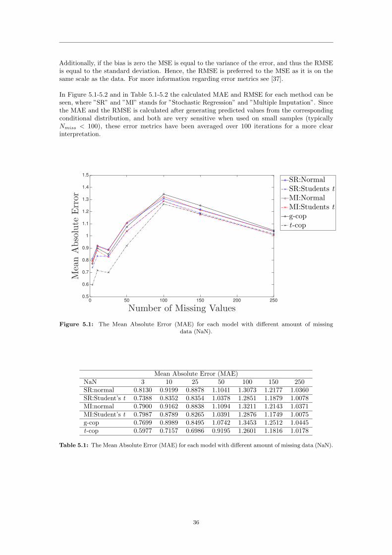
Additionally, if the bias is zero the MSE is equal to the variance of the error, and thus the RMSEis equal to the standard deviation. Hence, the RMSE is preferred to the MSE as it is on thesame scale as the data. For more information regarding error metrics see [37].
In Figure 5.1-5.2 and in Table 5.1-5.2 the calculated MAE and RMSE for each method can beseen, where ”SR” and ”MI” stands for ”Stochastic Regression” and ”Multiple Imputation”. Sincethe MAE and the RMSE is calculated after generating predicted values from the correspondingconditional distribution, and both are very sensitive when used on small samples (typicallyNmiss < 100), these error metrics have been averaged over 100 iterations for a more clearinterpretation.
Number of Missing Values0 50 100 150 200 250
MeanAbsolute
Error
0.5
0.6
0.7
0.8
0.9
1
1.1
1.2
1.3
1.4
1.5
SR:Normal
SR:Students t
MI:Normal
MI:Students t
g-cop
t-cop
Figure 5.1: The Mean Absolute Error (MAE) for each model with different amount of missingdata (NaN).
Mean Absolute Error (MAE)NaN 3 10 25 50 100 150 250SR:normal 0.8130 0.9199 0.8878 1.1041 1.3073 1.2177 1.0360SR:Student’s t 0.7388 0.8352 0.8354 1.0378 1.2851 1.1879 1.0078MI:normal 0.7900 0.9162 0.8838 1.1094 1.3211 1.2143 1.0371MI:Student’s t 0.7987 0.8789 0.8265 1.0391 1.2876 1.1749 1.0075g-cop 0.7699 0.8989 0.8495 1.0742 1.3453 1.2512 1.0445t-cop 0.5977 0.7157 0.6986 0.9195 1.2601 1.1816 1.0178
Table 5.1: The Mean Absolute Error (MAE) for each model with different amount of missing data (NaN).
36

Number of Missing Values0 50 100 150 200 250
RootMeanSquare
Error
0.8
1
1.2
1.4
1.6
1.8
2
SR:Normal
SR:Students t
MI:Normal
MI:Students t
g-cop
t-cop
Figure 5.2: The Root Mean Square Error (RMSE) for each model with different amount of missingdata (NaN).
Root Mean Square Error (RMSE)NaN 3 10 25 50 100 150 250SR:normal 0.9336 1.1233 1.1093 1.4988 1.7774 1.6385 1.4121SR:Student’s t 0.9025 1.0629 1.0889 1.4754 1.7632 1.6134 1.3900MI:normal 0.9224 1.1392 1.0984 1.5157 1.7894 1.6346 1.4131MI:Student’s t 0.9948 1.1311 1.1033 1.4685 1.7511 1.5962 1.3879g-cop 0.9170 1.0954 1.0527 1.4879 1.8404 1.7185 1.4527t-cop 0.7183 0.8822 0.8705 1.3129 1.7382 1.6095 1.4052
Table 5.2: The Root Mean Square Error (RMSE) for each model with different amount of missingdata (NaN).
37
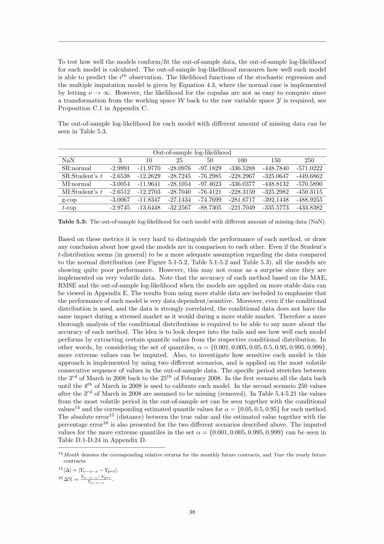
To test how well the models conform/fit the out-of-sample data, the out-of-sample log-likelihoodfor each model is calculated. The out-of-sample log-likelihood measures how well each modelis able to predict the ith observation. The likelihood functions of the stochastic regression andthe multiple imputation model is given by Equation 4.3, where the normal case is implementedby letting ν → ∞. However, the likelihood for the copulas are not as easy to compute sincea transformation from the working space W back to the raw variable space Y is required, seeProposition C.1 in Appendix C.
The out-of-sample log-likelihood for each model with different amount of missing data can beseen in Table 5.3.
Out-of-sample log-likelihoodNaN 3 10 25 50 100 150 250SR:normal -2.9991 -11.9770 -28.0976 -97.1829 -336.5288 -448.7840 -571.0222SR:Student’s t -2.6538 -12.2629 -28.7245 -76.2985 -228.2967 -325.0647 -449.6862MI:normal -3.0054 -11.9641 -28.1054 -97.4623 -336.0377 -448.8132 -570.5890MI:Student’s t -2.6512 -12.2703 -28.7040 -76.4121 -228.3159 -325.2982 -450.3115g-cop -3.0067 -11.8347 -27.1434 -74.7699 -281.6717 -392.1448 -488.9255t-cop -2.9745 -13.6448 -32.2567 -88.7305 -221.7049 -335.5773 -433.8382
Table 5.3: The out-of-sample log-likelihood for each model with different amount of missing data (NaN).
Based on these metrics it is very hard to distinguish the performance of each method, or drawany conclusion about how good the models are in comparison to each other. Even if the Student’st-distribution seems (in general) to be a more adequate assumption regarding the data comparedto the normal distribution (see Figure 5.1-5.2, Table 5.1-5.2 and Table 5.3), all the models areshowing quite poor performance. However, this may not come as a surprise since they areimplemented on very volatile data. Note that the accuracy of each method based on the MAE,RMSE and the out-of-sample log-likelihood when the models are applied on more stable data canbe viewed in Appendix E. The results from using more stable data are included to emphasize thatthe performance of each model is very data dependent/sensitive. Moreover, even if the conditionaldistribution is used, and the data is strongly correlated, the conditional data does not have thesame impact during a stressed market as it would during a more stable market. Therefore a morethorough analysis of the conditional distributions is required to be able to say more about theaccuracy of each method. The idea is to look deeper into the tails and see how well each modelperforms by extracting certain quantile values from the respective conditional distribution. Inother words, by considering the set of quantiles, α = {0.001, 0.005, 0.05, 0.5, 0.95, 0.995, 0.999},more extreme values can be imputed. Also, to investigate how sensitive each model is thisapproach is implemented by using two different scenarios, and is applied on the most volatileconsecutive sequence of values in the out-of-sample data. The specific period stretches betweenthe 3rd of March in 2008 back to the 25th of Feburary 2008. In the first scenario all the data backuntil the 4th of March in 2008 is used to calibrate each model. In the second scenario 250 valuesafter the 3rd of March in 2008 are assumed to be missing (removed). In Table 5.4-5.21 the valuesfrom the most volatile period in the out-of-sample set can be seen together with the conditionalvalues14 and the corresponding estimated quantile values for α = {0.05, 0.5, 0.95} for each method.The absolute error15 (distance) between the true value and the estimated value together with thepercentage error16 is also presented for the two different scenarios described above. The imputedvalues for the more extreme quantiles in the set α = {0.001, 0.005, 0.995, 0.999} can be seen inTable D.1-D.24 in Appendix D.
14 Month denotes the corresponding relative returns for the monthly future contracts, and Year the yearly futurecontracts.
15 |∆| = |Yo−o−s − Ypre|.16 ∆% =
Yo−o−s−YpreYo−o−s
.
38

SR:normal, α = 0.95Nmiss = 0 Nmiss = 250
Date Monthly Yearly Yo−o−s Ypre |∆| ∆% Ypre |∆| ∆%2008-03-03 -7.9176 -2.4645 -10.3876 -4.4107 5.9769 0.5754 -4.5136 5.8740 0.56552008-02-29 -4.8392 0 -5.9767 -1.3406 4.6361 0.7757 -1.4499 4.5268 0.75742008-02-28 0.4615 0.3806 1.3294 1.8233 0.4939 -0.3716 1.5231 0.1937 -0.14572008-02-27 7.4380 2.5366 7.4603 6.8969 0.5634 0.0755 6.4223 1.0380 0.13912008-02-26 -6.3467 -2.6591 -7.6246 -3.6420 3.9826 0.5223 -3.8158 3.8089 0.49952008-02-25 -7.7143 -0.5666 -8.2100 -3.2545 4.9554 0.6036 -3.2771 4.9329 0.6008
Table 5.4: An overview of the values from the most volatile period in the out-of-sample set together withthe conditional values, and the corresponding estimated quantile values for α = 0.95 for the SR:normalmethod. The absolute error (distance) between the true value and the estimated value together with the
percentage error is also presented for two different scenarios.
SR:normal, α = 0.5Nmiss = 0 Nmiss = 250
Date Monthly Yearly Yo−o−s Ypre |∆| ∆% Ypre |∆| ∆%2008-03-03 -7.9176 -2.4645 -10.3876 -5.7323 4.6553 0.4482 -5.5538 4.8338 0.46532008-02-29 -4.8392 0 -5.9767 -2.6622 3.3145 0.5546 -2.4902 3.4865 0.58342008-02-28 0.4615 0.3806 1.3294 0.5017 0.8277 0.6226 0.4828 0.8466 0.63682008-02-27 7.4380 2.5366 7.4603 5.5753 1.8850 0.2527 5.3821 2.0782 0.27862008-02-26 -6.3467 -2.6591 -7.6246 -4.9636 2.6610 0.3490 -4.8560 2.7687 0.36312008-02-25 -7.7143 -0.5666 -8.2100 -4.5761 3.6338 0.4426 -4.3173 3.8926 0.4741
Table 5.5: An overview of the values from the most volatile period in the out-of-sample set together withthe conditional values, and the corresponding estimated quantile values for α = 0.5 for the SR:normalmethod. The absolute error (distance) between the true value and the estimated value together with the
percentage error is also presented for two different scenarios.
SR:normal, α = 0.05Nmiss = 0 Nmiss = 250
Date Monthly Yearly Yo−o−s Ypre |∆| ∆% Ypre |∆| ∆%2008-03-03 -7.9176 -2.4645 -10.3876 -7.0539 3.3337 0.3209 -6.5940 3.7936 0.36522008-02-29 -4.8392 0 -5.9767 -3.9838 1.9929 0.3334 -3.5304 2.4463 0.40932008-02-28 0.4615 0.3806 1.3294 -0.8199 2.1493 1.6167 -0.5574 1.8868 1.41932008-02-27 7.4380 2.5366 7.4603 4.2537 3.2066 0.4298 4.3419 3.1184 0.41802008-02-26 -6.3467 -2.6591 -7.6246 -6.2852 1.3394 0.1757 -5.8962 1.7284 0.22672008-02-25 -7.7143 -0.5666 -8.2100 -5.8977 2.3122 0.2816 -5.3575 2.8524 0.3474
Table 5.6: An overview of the values from the most volatile period in the out-of-sample set together withthe conditional values, and the corresponding estimated quantile values for α = 0.05 for the SR:normalmethod. The absolute error (distance) between the true value and the estimated value together with the
percentage error is also presented for two different scenarios.
39

SR:Student’s t, α = 0.95Nmiss = 0 Nmiss = 250
Date Monthly Yearly Yo−o−s Ypre |∆| ∆% Ypre |∆| ∆%2008-03-03 -7.9176 -2.4645 -10.3876 -4.6754 5.7122 0.5499 -4.6151 5.7724 0.55572008-02-29 -4.8392 0 -5.9767 -1.6094 4.3673 0.7307 -1.5601 4.4165 0.73902008-02-28 0.4615 0.3806 1.3294 1.6782 0.3488 -0.2624 1.4767 0.1473 -0.11082008-02-27 7.4380 2.5366 7.4603 6.8586 0.6018 0.0807 6.4262 1.0341 0.13862008-02-26 -6.3467 -2.6591 -7.6246 -3.8597 3.7650 0.4938 -3.8921 3.7325 0.48952008-02-25 -7.7143 -0.5666 -8.2100 -3.5783 4.6317 0.5642 -3.4146 4.7954 0.5841
Table 5.7: An overview of the values from the most volatile period in the out-of-sample set together withthe conditional values, and the corresponding estimated quantile values for α = 0.95 for the SR:Student’st method. The absolute error (distance) between the true value and the estimated value together with
the percentage error is also presented for two different scenarios.
SR:Student’s t, α = 0.5Nmiss = 0 Nmiss = 250
Date Monthly Yearly Yo−o−s Ypre |∆| ∆% Ypre |∆| ∆%2008-03-03 -7.9176 -2.4645 -10.3876 -5.8722 4.5154 0.4347 -5.6107 4.7769 0.45992008-02-29 -4.8392 0 -5.9767 -2.8062 3.1705 0.5305 -2.5557 3.4210 0.57242008-02-28 0.4615 0.3806 1.3294 0.4814 0.8480 0.6379 0.4811 0.8483 0.63812008-02-27 7.4380 2.5366 7.4603 5.6618 1.7985 0.2411 5.4307 2.0296 0.27212008-02-26 -6.3467 -2.6591 -7.6246 -5.0564 2.5682 0.3368 -4.8877 2.7370 0.35902008-02-25 -7.7143 -0.5666 -8.2100 -4.7751 3.4349 0.4184 -4.4101 3.7998 0.4628
Table 5.8: An overview of the values from the most volatile period in the out-of-sample set together withthe conditional values, and the corresponding estimated quantile values for α = 0.5 for the SR:Student’st method. The absolute error (distance) between the true value and the estimated value together with
the percentage error is also presented for two different scenarios.
SR:Student’s t, α = 0.05Nmiss = 0 Nmiss = 250
Date Monthly Yearly Yo−o−s Ypre |∆| ∆% Ypre |∆| ∆%2008-03-03 -7.9176 -2.4645 -10.3876 -7.0690 3.3186 0.3195 -6.6062 3.7814 0.36402008-02-29 -4.8392 0 -5.9767 -4.0030 1.9737 0.3302 -3.5512 2.4255 0.40582008-02-28 0.4615 0.3806 1.3294 -0.7153 2.0447 1.5381 -0.5144 1.8438 1.38692008-02-27 7.4380 2.5366 7.4603 4.4650 2.9953 0.4015 4.4352 3.0251 0.40552008-02-26 -6.3467 -2.6591 -7.6246 -6.2532 1.3714 0.1799 -5.8832 1.7414 0.22842008-02-25 -7.7143 -0.5666 -8.2100 -5.9719 2.2381 0.2726 -5.4057 2.8043 0.3416
Table 5.9: An overview of the values from the most volatile period in the out-of-sample set together withthe conditional values, and the corresponding estimated quantile values for α = 0.05 for the SR:Student’st method. The absolute error (distance) between the true value and the estimated value together with
the percentage error is also presented for two different scenarios.
40

MI:normal, α = 0.95Nmiss = 0 Nmiss = 250
Date Monthly Yearly Yo−o−s Ypre |∆| ∆% Ypre |∆| ∆%2008-03-03 -7.9176 -2.4645 -10.3876 -4.4163 5.9713 0.5748 -4.4920 5.8956 0.56762008-02-29 -4.8392 0 -5.9767 -1.3384 4.6382 0.7761 -1.4267 4.5500 0.76132008-02-28 0.4615 0.3806 1.3294 1.8261 0.4967 -0.3736 1.5293 0.1999 -0.15032008-02-27 7.4380 2.5366 7.4603 6.9058 0.5545 0.0743 6.4146 1.0457 0.14022008-02-26 -6.3467 -2.6591 -7.6246 -3.6485 3.9762 0.5215 -3.8008 3.8238 0.50152008-02-25 -7.7143 -0.5666 -8.2100 -3.2539 4.9560 0.6037 -3.2465 4.9635 0.6046
Table 5.10: An overview of the values from the most volatile period in the out-of-sample set togetherwith the conditional values, and the corresponding estimated quantile values for α = 0.95 for theMI:normal method. The absolute error (distance) between the true value and the estimated value
together with the percentage error is also presented for two different scenarios.
MI:normal, α = 0.5Nmiss = 0 Nmiss = 250
Date Monthly Yearly Yo−o−s Ypre |∆| ∆% Ypre |∆| ∆%2008-03-03 -7.9176 -2.4645 -10.3876 -5.7180 4.6696 0.4495 -5.5226 4.8650 0.46842008-02-29 -4.8392 0 -5.9767 -2.6501 3.3266 0.5566 -2.4619 3.5148 0.58812008-02-28 0.4615 0.3806 1.3294 0.5071 0.8223 0.6186 0.4927 0.8367 0.62942008-02-27 7.4380 2.5366 7.4603 5.5730 1.8873 0.2530 5.3735 2.0868 0.27972008-02-26 -6.3467 -2.6591 -7.6246 -4.9515 2.6731 0.3506 -4.8313 2.7934 0.36642008-02-25 -7.7143 -0.5666 -8.2100 -4.5607 3.6493 0.4445 -4.2803 3.9297 0.4786
Table 5.11: An overview of the values from the most volatile period in the out-of-sample set togetherwith the conditional values, and the corresponding estimated quantile values for α = 0.5 for the MI:normalmethod. The absolute error (distance) between the true value and the estimated value together with the
percentage error is also presented for two different scenarios.
MI:normal, α = 0.05Nmiss = 0 Nmiss = 250
Date Monthly Yearly Yo−o−s Ypre |∆| ∆% Ypre |∆| ∆%2008-03-03 -7.9176 -2.4645 -10.3876 -7.0585 3.3291 0.3205 -6.5621 3.8255 0.36832008-02-29 -4.8392 0 -5.9767 -3.9866 1.9901 0.3330 -3.5017 2.4749 0.41412008-02-28 0.4615 0.3806 1.3294 -0.8206 2.1500 1.6173 -0.5511 1.8805 1.41462008-02-27 7.4380 2.5366 7.4603 4.2561 3.2042 0.4295 4.3258 3.1345 0.42022008-02-26 -6.3467 -2.6591 -7.6246 -6.2892 1.3354 0.1751 -5.8722 1.7524 0.22982008-02-25 -7.7143 -0.5666 -8.2100 -5.9018 2.3081 0.2811 -5.3183 2.8916 0.3522
Table 5.12: An overview of the values from the most volatile period in the out-of-sample set togetherwith the conditional values, and the corresponding estimated quantile values for α = 0.05 for theMI:normal method. The absolute error (distance) between the true value and the estimated value
together with the percentage error is also presented for two different scenarios.
41

MI:Student’s t, α = 0.95Nmiss = 0 Nmiss = 250
Date Monthly Yearly Yo−o−s Ypre |∆| ∆% Ypre |∆| ∆%2008-03-03 -7.9176 -2.4645 -10.3876 -2.9315 7.4561 0.7178 -4.5888 5.7988 0.55822008-02-29 -4.8392 0 -5.9767 0.1342 6.1108 1.0224 -1.6037 4.3729 0.73172008-02-28 0.4615 0.3806 1.3294 3.4165 2.0871 -1.5700 1.4619 0.1325 -0.09972008-02-27 7.4380 2.5366 7.4603 8.5919 1.1316 -0.1517 6.3855 1.0748 0.14412008-02-26 -6.3467 -2.6591 -7.6246 -2.1177 5.5070 0.7223 -3.8454 3.7792 0.49572008-02-25 -7.7143 -0.5666 -8.2100 -1.8323 6.3777 0.7768 -3.4599 4.7500 0.5786
Table 5.13: An overview of the values from the most volatile period in the out-of-sample set togetherwith the conditional values, and the corresponding estimated quantile values for α = 0.95 for theMI:Student’s t method. The absolute error (distance) between the true value and the estimated value
together with the percentage error is also presented for two different scenarios.
MI:Student’s t, α = 0.5Nmiss = 0 Nmiss = 250
Date Monthly Yearly Yo−o−s Ypre |∆| ∆% Ypre |∆| ∆%2008-03-03 -7.9176 -2.4645 -10.3876 -5.8754 4.5122 0.4344 -5.5796 4.8080 0.46292008-02-29 -4.8392 0 -5.9767 -2.8076 3.1691 0.5302 -2.5964 3.3802 0.56562008-02-28 0.4615 0.3806 1.3294 0.4820 0.8473 0.6374 0.4614 0.8680 0.65302008-02-27 7.4380 2.5366 7.4603 5.6655 1.7948 0.2406 5.3766 2.0837 0.27932008-02-26 -6.3467 -2.6591 -7.6246 -5.0591 2.5655 0.3365 -4.8389 2.7857 0.36542008-02-25 -7.7143 -0.5666 -8.2100 -4.7776 3.4323 0.4181 -4.4488 3.7612 0.4581
Table 5.14: An overview of the values from the most volatile period in the out-of-sample set together withthe conditional values, and the corresponding estimated quantile values for α = 0.5 for the MI:Student’st method. The absolute error (distance) between the true value and the estimated value together with
the percentage error is also presented for two different scenarios.
MI:Student’s t, α = 0.05Nmiss = 0 Nmiss = 250
Date Monthly Yearly Yo−o−s Ypre |∆| ∆% Ypre |∆| ∆%2008-03-03 -7.9176 -2.4645 -10.3876 -7.0711 3.3165 0.3193 -6.5805 3.8071 0.36652008-02-29 -4.8392 0 -5.9767 -4.0036 1.9730 0.3301 -3.5949 2.3818 0.39852008-02-28 0.4615 0.3806 1.3294 -0.7149 2.0443 1.5378 -0.5379 1.8673 1.40472008-02-27 7.4380 2.5366 7.4603 4.4674 2.9929 0.4012 4.3783 3.0820 0.41312008-02-26 -6.3467 -2.6591 -7.6246 -6.2551 1.3695 0.1796 -5.8404 1.7842 0.23402008-02-25 -7.7143 -0.5666 -8.2100 -5.9732 2.2367 0.2724 -5.4472 2.7628 0.3365
Table 5.15: An overview of the values from the most volatile period in the out-of-sample set togetherwith the conditional values, and the corresponding estimated quantile values for α = 0.05 for theMI:Student’s t method. The absolute error (distance) between the true value and the estimated value
together with the percentage error is also presented for two different scenarios.
42

g-cop, α = 0.95Nmiss = 0 Nmiss = 250
Date Monthly Yearly Yo−o−s Ypre |∆| ∆% Ypre |∆| ∆%2008-03-03 -7.9176 -2.4645 -10.3876 -4.2304 6.1572 0.5927 -4.3909 5.9967 0.57732008-02-29 -4.8392 0 -5.9767 -1.4468 4.5299 0.7579 -1.4808 4.4959 0.75222008-02-28 0.4615 0.3806 1.3294 1.7823 0.4529 0.3407 1.4994 0.1700 0.12792008-02-27 7.4380 2.5366 7.4603 7.3363 0.1241 0.0166 6.7530 0.7073 0.09482008-02-26 -6.3467 -2.6591 -7.6246 -3.6314 3.9932 0.5237 -3.7924 3.8322 0.50262008-02-25 -7.7143 -0.5666 -8.2100 -3.0412 5.1687 0.6296 -3.0559 5.1541 0.6278
Table 5.16: An overview of the values from the most volatile period in the out-of-sample set togetherwith the conditional values, and the corresponding estimated quantile values for α = 0.95 for the g-copulamethod. The absolute error (distance) between the true value and the estimated value together with the
percentage error is also presented for two different scenarios.
g-cop, α = 0.5Nmiss = 0 Nmiss = 250
Date Monthly Yearly Yo−o−s Ypre |∆| ∆% Ypre |∆| ∆%2008-03-03 -7.9176 -2.4645 -10.3876 -5.7383 4.6493 0.4476 -5.7453 4.6423 0.44692008-02-29 -4.8392 0 -5.9767 -2.6817 3.2950 0.5513 -2.5241 3.4526 0.57772008-02-28 0.4615 0.3806 1.3294 0.5522 0.7772 0.5846 0.5399 0.7895 0.59392008-02-27 7.4380 2.5366 7.4603 5.5107 1.9497 0.2613 5.2722 2.1881 0.29332008-02-26 -6.3467 -2.6591 -7.6246 -5.0631 2.5615 0.3359 -5.0473 2.5774 0.33802008-02-25 -7.7143 -0.5666 -8.2100 -4.4069 3.8030 0.4632 -4.2660 3.9440 0.4804
Table 5.17: An overview of the values from the most volatile period in the out-of-sample set togetherwith the conditional values, and the corresponding estimated quantile values for α = 0.5 for the g-copulamethod. The absolute error (distance) between the true value and the estimated value together with the
percentage error is also presented for two different scenarios.
g-cop, α = 0.05Nmiss = 0 Nmiss = 250
Date Monthly Yearly Yo−o−s Ypre |∆| ∆% Ypre |∆| ∆%2008-03-03 -7.9176 -2.4645 -10.3876 -7.4611 2.9265 0.2817 -7.3039 3.0837 0.29692008-02-29 -4.8392 0 -5.9767 -4.0092 1.9675 0.3292 -3.6225 2.3542 0.39392008-02-28 0.4615 0.3806 1.3294 -0.6387 1.9681 1.4805 -0.3821 1.7115 1.28742008-02-27 7.4380 2.5366 7.4603 3.9256 3.5348 0.4738 4.0158 3.4445 0.46172008-02-26 -6.3467 -2.6591 -7.6246 -6.6826 0.9420 0.1236 -6.4893 1.1353 0.14892008-02-25 -7.7143 -0.5666 -8.2100 -5.9350 2.2750 0.2771 -5.5921 2.6179 0.3189
Table 5.18: An overview of the values from the most volatile period in the out-of-sample set togetherwith the conditional values, and the corresponding estimated quantile values for α = 0.05 for the g-copulamethod. The absolute error (distance) between the true value and the estimated value together with the
percentage error is also presented for two different scenarios.
43

t-cop, α = 0.95Nmiss = 0 Nmiss = 250
Date Monthly Yearly Yo−o−s Ypre |∆| ∆% Ypre |∆| ∆%2008-03-03 -7.9176 -2.4645 -10.3876 -4.9212 5.4664 0.5262 -4.3924 5.9952 0.57722008-02-29 -4.8392 0 -5.9767 -2.0292 3.9474 0.6605 -1.4568 4.5199 0.75632008-02-28 0.4615 0.3806 1.3294 1.2423 0.0871 0.0655 1.5377 0.2083 0.15672008-02-27 7.4380 2.5366 7.4603 6.2975 1.1628 0.1559 6.1186 1.3417 0.17982008-02-26 -6.3467 -2.6591 -7.6246 -4.2011 3.4236 0.4490 -3.7665 3.8582 0.50602008-02-25 -7.7143 -0.5666 -8.2100 -3.9074 4.3025 0.5241 -3.2295 4.9805 0.6066
Table 5.19: An overview of the values from the most volatile period in the out-of-sample set togetherwith the conditional values, and the corresponding estimated quantile values for α = 0.95 for the t-copulamethod. The absolute error (distance) between the true value and the estimated value together with the
percentage error is also presented for two different scenarios.
t-cop, α = 0.5Nmiss = 0 Nmiss = 250
Date Monthly Yearly Yo−o−s Ypre |∆| ∆% Ypre |∆| ∆%2008-03-03 -7.9176 -2.4645 -10.3876 -5.8175 4.5701 0.4400 -5.7156 4.6720 0.44982008-02-29 -4.8392 0 -5.9767 -2.9775 2.9991 0.5018 -2.8468 3.1299 0.52372008-02-28 0.4615 0.3806 1.3294 0.5076 0.8217 0.6181 0.5080 0.8214 0.61792008-02-27 7.4380 2.5366 7.4603 5.4621 1.9982 0.2678 5.1876 2.2727 0.30462008-02-26 -6.3467 -2.6591 -7.6246 -5.0123 2.6124 0.3426 -4.9805 2.6441 0.34682008-02-25 -7.7143 -0.5666 -8.2100 -4.9899 3.2201 0.3922 -4.8050 3.4049 0.4147
Table 5.20: An overview of the values from the most volatile period in the out-of-sample set togetherwith the conditional values, and the corresponding estimated quantile values for α = 0.5 for the t-copulamethod. The absolute error (distance) between the true value and the estimated value together with the
percentage error is also presented for two different scenarios.
t-cop, α = 0.05Nmiss = 0 Nmiss = 250
Date Monthly Yearly Yo−o−s Ypre |∆| ∆% Ypre |∆| ∆%2008-03-03 -7.9176 -2.4645 -10.3876 -6.6062 3.7814 0.3640 -6.7073 3.6803 0.35432008-02-29 -4.8392 0 -5.9767 -3.8308 2.1459 0.3590 -4.0086 1.9681 0.32932008-02-28 0.4615 0.3806 1.3294 -0.2210 1.5504 1.1662 -0.5444 1.8738 1.40952008-02-27 7.4380 2.5366 7.4603 4.5426 2.9178 0.3911 3.9672 3.4931 0.46822008-02-26 -6.3467 -2.6591 -7.6246 -5.7389 1.8857 0.2473 -5.8987 1.7260 0.22642008-02-25 -7.7143 -0.5666 -8.2100 -5.9278 2.2821 0.2780 -6.0259 2.1840 0.2660
Table 5.21: An overview of the values from the most volatile period in the out-of-sample set togetherwith the conditional values, and the corresponding estimated quantile values for α = 0.05 for the t-copulamethod. The absolute error (distance) between the true value and the estimated value together with the
percentage error is also presented for two different scenarios.
44

By investigating Table 5.4-5.21 and Table D.1-D.24, it can be seen that the performance ofeach method can be significantly increased by imputing more extreme quantile values. Byletting the median (α = 0.5) of the corresponding conditional distribution be a representative forthe standard method (where samples are randomly drawn from the corresponding conditionaldistribution), the standard method can be compared with the approach of imputing more extremequantile values. In Figure 5.1-5.2 and Table 5.1-5.2 it can be seen that the standard method isinsufficient when applied on more volatile data. However, the standard approach can be usedto compute a first estimate of the final imputed value. This value can then be substituted bylower extreme values (α = 0.05) or higher extreme values (α = 0.95) depending on whether thecorresponding conditional values are greater or smaller then this first estimate. In other words,the results in Table 5.4-5.21 and Table D.1-D.24 indicate that it is required to extract lowerquantile values if the median value is greater than the corresponding Monthly future value, andvice versa. Even if there is an obvious trend in the results the dependence structure regardingthe conditional values, quantile values and median values is very vague and requires to be morethoroughly analyzed before any real conclusions can be made.
Additionally, by calculating the absolute difference between the percentage error (∆%) forNmiss = 0 and Nmiss = 250 it can be concluded that the g-copula and t-copula models are morerobust than the respective linear models, see Table 5.22.
|∆%Nmiss=0 −∆%Nmiss=250|α 0.999 0.995 0.95 0.5 0.05 0.005 0.001 AverageSR:normal 0.1150 0.0944 0.0572 0.0219 0.0744 0.1116 0.1322 0.1011SR:Student’s t 0.6452 0.2646 0.0413 0.0275 0.0655 0.2988 0.6794 0.2889MI:normal 0.1131 0.0917 0.0554 0.0230 0.0778 0.1167 0.1363 0.0877MI:Student’s t 0.5839 0.2670 0.4402 0.0312 0.0632 0.2927 0.6725 0.3358g-cop 0.1178 0.1041 0.0558 0.0146 0.0587 0.0912 0.1193 0.0802t-cop 0.2348 0.1862 0.0669 0.0159 0.0655 0.1371 0.1739 0.1257
Table 5.22: The mean absolute difference (MD) between the percentage error (∆%) for Nmiss = 0 andNmiss = 250.
Although the more heavy tailed assumption in general seems to be more accurate (see Figure 5.1-5.2 and Table 5.1-5.2), using the g-copula and impute values from the extreme quantile α = 0.0001seems to give very satisfying results, see Table 5.23.
g-cop, α = 0.0001Nmiss = 0 Nmiss = 250
Date Monthly Yearly Yo−o−s Ypre |∆| ∆% Ypre |∆| ∆%2008-03-03 -7.9176 -2.4645 -10.3876 -10.0661 0.3215 0.0309 -9.7969 0.5907 0.05692008-02-29 -4.8392 0 -5.9767 -5.9064 0.0702 0.0118 -5.2828 0.6939 0.11612008-02-28 0.4615 0.3806 1.3294 -2.1607 3.4901 2.6253 -1.6686 2.9980 2.25522008-02-27 7.4380 2.5366 7.4603 2.1809 5.2794 0.7077 2.4865 4.9738 0.66672008-02-26 -6.3467 -2.6591 -7.6246 -9.1100 1.4854 0.1948 -8.8006 1.1760 0.15422008-02-25 -7.7143 -0.5666 -8.2100 -8.2017 0.0083 0.0010 -7.6464 0.5636 0.0686
Table 5.23: An overview of the values from the most volatile period in the out-of-sample set togetherwith the conditional values, and the corresponding estimated quantile values for α = 0.0001 for theg-copula method. The absolute error (distance) between the true value and the estimated value together
with the percentage error is also presented for two different scenarios.
45

Chapter 6
Conclusions
In this thesis three different methods have been investigated for imputation of missing dataconcerning commodity futures returns in the context of the preparatory work regarding stresstesting. To retain the variability of the data the chosen approach has been to impute historicalreturn data by the conditional distribution rather than the conditional expectation. This approachalso has the advantage that certain extreme quantile values can be extracted from each parametricmodel, and used in different stress testing scenarios.
The two first models implemented in this paper are currently regarded as state-of-the-art tech-niques for managing missing data. The first method, Stochastic Regression Imputation, uses aBayesian approach to find the corresponding MAP-estimate of the coefficients in the regressionequation. The second model, Multiple Imputation (MI), uses a full17 implementation of theBayesian theory, and by simulation generates new covariances and mean values used to con-struct multiple sets of augmented data chains. Although the first and second approach tendto produce similar results when the regression equations includes the same variables, the latterhas the advantage of not depending solely on one imputed value for each missing data event.The third alternative method implemented in this thesis is based on elliptical copulas and thebeneficial properties of the Arellano-Valle and Bolfarine’s generalized t-distribution [21]. Incontrast to the first two approaches the marginal distribution of each random variable is mod-elled separately, and the dependence structure is applied in a non-linear manner in the third model.
The characteristics of the data is known to be non-normal. However, both a normal distributionand a more heavy tailed assumption, in form of a t-distribution, has been assigned to the missingdata to study the validity of the model assumptions for each method separately. However, it iswell known that the normal assumption is a very naive approach since it does not regard anypossible tail dependence. This means that the probability that two random variables simultan-eously attain extreme values is zero, even if the variables are correlated. In contrast, the taildependence under the t-distribution increases with correlation, and decreases when the numberof degrees of freedom increases. However, to attain the accuracy of each method more thoroughlysome conventional error metrics like the Mean Absolute Error, Root Mean Square Error andout-of-sample log-likelihood are used.
Based on these metrics it is very hard to distinguish the performance of each method, or draw anyconclusion about how good the models are in comparison to each other. Even if the Student’s t-distribution seems (in general) to be a more adequate assumption regarding the data compared tothe normal distribution (see Figure 5.1-5.2, Table 5.1-5.2 and Table 5.3), all the models are show-ing quite poor performance. However, by analyzing the conditional distributions more thoroughly,i.e. by looking deeper into the tails and extracting more extreme quantile values the performanceof each method is increased significantly. Additionally, by calculating the absolute differencebetween the percentage error (∆%) for Nmiss = 0 and Nmiss = 250 it can be concluded thatthe g-copula and t-copula models are more robust than the respective linear models, see Table 5.22.
Note, even if the results in Table 5.4-5.21, Table 5.23 and Table D.1-D.24 show very goodperformance the models are calibrated when the true data is known. Hence, these results are
17 In the sense that the distribution of each parameter is considered and not only a single estimate.
46

just presented to show that the models can actually perform very well if the distributions aremore thoroughly investigated. Therefore, an important and interesting topic for future studieswould be to investigate how sensitive the conditional distributions are, concerning the conditionaldata, to see how far into the tails it is required to go before any reasonable results can be obtained.
Moreover, the aim of this thesis has been to provide a more sophisticated method used to imputemissing historical data in the preparatory work of portfolio stress testing. However, the methodsused are only implemented on one type of data and missing data pattern. Hence, in the future itwould be interesting to apply these methods on a broader set of data/financial instruments, andin a context where the missing data is missing in a non-monotone univariate pattern.
Finally, a natural way of proceeding this work would be to investigate the influence theseimputation methods have on the profit and loss distribution compared to current routines. Inother words, it would be interesting to see how the expected future losses and the amount ofcapital needed to be secured is affected when these new tractable methods are implemented inthe context of portfolio stress testing.
47

Bibliography
[1] Burden, R. L. and Faires, J. D. 2011.Solutions of Equations in One Variable - The BisectionMethod. Beamer Presentation Slides prepared by John Carroll Dublin City University. Available at:https://www.math.ust.hk/∼mamu/courses/231/Slides/ch02 1.pdf, (Retrieved 2016-02-26).
[2] Carter, Tom. 2014. An introduction to information theory and entropy. California State University.Available at: http://csustan.csustan.edu/∼tom/Lecture-Notes/Information-Theory/info-lec.pdf,(Retrieved 2016-01-20).
[3] Chakrabarti, Brato. 2011. Bisection Method.Available at: http://www.mathworks.com/matlabcentral/fileexchange/33748-bisection-method/all files, (Retrieved 2016-02-26).
[4] Dall’Aglio, G., Kotz, S., Salinetti, G. 1991. Advances In Probability Distributions with GivenMarginals : Beyond the Copulas. Vol. 67. Dordrecht: Springer Science+Business Media Dordrecht.
[5] Demarta, Stefano and McNeil, Alexander J. 2004. The t Copula and Related Copulas. Departmentof Mathematics Federal Institute of Technology, ETH, Zurich.Available at: http://clone.risknet.de/fileadmin/eLibrary/t-Copula-Demarta-ETH.pdf,(Retrieved 2016-01-20).
[6] Dempster, Arthur P., Laird, Nan M. and Dempster, A., and Rubin, Donald B. 1977. MaximumLikelihood from Incomplete Data via the EM Algorithm. Journal of the Royal Statistical Society.Series B (Methodological), Vol. 39, No. 1, pp. 1-38.
[7] Embrechts, Paul, Lindskog, Filip and McNeil, Alexander. 2001. Modelling Dependence with Copulasand Applications to Risk Management. Department of Mathematics, ETHZ, CH-8092 Zurich,Switzerland. Available at: https://people.math.ethz.ch/∼embrecht/ftp/copchapter.pdf,(Retrieved 2016-01-17).
[8] Embrechts, P., McNeil A. and Straumann D. 2009. Correlation and Dependency in Risk Management:Properties and Pitfalls. The Journal of Risk and Insurance. Series B, Vol. 76, No. 3, pp. 639-650.
[9] Embrechts, Paul. 2009. Copulas: A Personal View. The Journal of Risk and Insurance. Series B,Vol. 76, No. 3, pp. 639-650.
[10] Enders, Craig K. 2010. Applied Missing Data Analysis. New York: The Guilford Press.
[11] European Securities and Markets Authority. 2015. WHO WE ARE.Available at: https://www.esma.europa.eu/about-esma/who-we-are, (Retrieved 2016-01-20).
[12] European Securities and Markets Authority. 2015. 2016 Work Programme.Available at: https://www.esma.europa.eu/sites/default/files/library/2015/10/2015-1475 esma2016 work programme.pdf, (Retrieved 2016-01-20).
[13] Friedman, C., Huang, J., Zhang, Y. and Cao, W. 2009. Joint and conditional transformed t-mixturemodels with applications to financial and economic data. The Journal of Risk, Vol. 11, No. 3, pp.25-54.
[14] Friedman, C., Huang, J., Zhang, Y. and Cao, W. 2012. Missing value imputation via copula andtransformation methods, with applications to financial and economic data. Int. J. Data AnalysisTechniques and Strategies, Vol. 4, No. 4, pp. 315-339.
48

[15] Frost, Jim. 2013. Regression Analysis: How to Interpret the Constant (Y Intercept). The Min-itab Blog. [Blog]. 11 July. Available at: http://blog.minitab.com/blog/adventures-in-statistics/regression-analysis-how-to-interpret-the-constant-y-intercept, (Retrieved 2015-11-11).
[16] Hansen, Bruce E. 2000. Econometrics. University of Wisconsin.Available at: http://www.ssc.wisc.edu/∼bhansen/econometrics/, (Retrieved 2016-01-20).
[17] Hedensio, Martin. 2014. NASDAQ OMX CLEARING RECEIVES EMIR AUTHORISATION.NASDAQ OMX. Available at: http://www.nasdaqomx.com/newsroom/pressreleases/pressrelease?messageId=1253167&displayLanguage=en, (Retrieved 2016-01-20).
[18] Jones, D. L. 2014. The Johnson Curve Toolbox for Matlab: analysis of non-normal data usingthe Johnson system of distributions. College of Marine Science, University of South Florida, St.Petersburg, Florida, USA. Available at: http://www.mathworks.com/matlabcentral/fileexchange/46123-johnson-curve-toolbox, (Retrieved 2016-01-17).
[19] Kaarik, Ene. 2005. Handling dropouts by copulas. WSEAS Transactions on Biology and Biomedicine,Vol. 1, No. 2, pp. 93-97.
[20] Kaarik, Ene. 2006. Imputation Algorithm Using Copulas. Metodoloski zvezki, Vol. 3, No. 1, pp.109-120.
[21] Kotz, S. and Nadarajah S. 2004. Multivariate t-Distributions and Their Applications. Cambridge.
[22] Lang, Harald. 2014. Elements of Regression Analysis. Royal Institute of Technology, Stockholm.
[23] Liu, Chuanhai. 1994. Statistical Analysis Using the Multivariate t Distribution. Department ofStatistics Harvard University. Available at: www.geog.ucsb.edu/∼dongmei/chuanhai.ps, (Retrieved2016-02-15).
[24] McNeil, Alexander J., Rudiger Frey., Embrechts Paul. 2005. Quantitative Risk Management: Con-cepts, techniques and Tools. Princeton and Oxford: Princeton University Press.
[25] Meng, Xiao L. and Rubin, Donald B. 1993. Maximum Likelihood via the ECM Algorithm: A GeneralFramework. Biometrika, Vol. 80, No. 2, pp. 267-278.
[26] NASDAQ OMX Group. April 2015. NASDAQ Clearing as a Counterparty. Available at: http://www.nasdaqomx.com/digitalAssets/98/98491 nasdaq-clearing-as-a-counterparty-april-2015.pdf,(Retrieved 2016-01-20).
[27] Nelsen, Roger B. 2006. An Introduction to Copulas. 2nd. Ed. New York: Springer.
[28] Olsson, Jimmy. 2014. SF2955 Computer Intensive Methods in Mathematical Statistics [Examand Solutions]. Department of mathematics, Royal Institute of Technology (KTH), Stockholm.Available at: https://www.math.kth.se/matstat/gru/sf2955/Exam/exam SF2955 20140818.pdf andhttps://www.math.kth.se/matstat/gru/sf2955/Exam/exam SF2955 20140818 solutions.pdf(Retrieved 2016-04-20).
[29] Peel, David and Mclachlan, Geoffrey J. 2000. Robust mixture modelling using the t distributions.Statistics and Computing, Vol. 10, No. 4, pp. 339-348.
[30] Piche, Robert. 2011. Robust multivariate linear regression using the Student-t distribution. Pro-fessor of Automation Science and Engineering at Tampere University of Technology. Availableat: http://www.mathworks.com/matlabcentral/fileexchange/38212-mvsregress/content/mvsregresspackage/mvsregress.m, (Retrieved 2016-01-17).
[31] Robert, Christian P. and Casella, George. 2004. Monte Carlo Statistical Methods. 2nd. Ed. NewYork: Springer.
[32] Roth, Michael. 2013. On the Multivariate t Distribution. Technical report from Automatic Controlat Linkopings University. Available at: http://users.isy.liu.se/en/rt/roth/student.pdf,(Retrieved 2016-02-15).
[33] Lindgren, Georg, Rootzen, Holger and Sandsten, Maria. 2013. Appendix A Some Probabilityand Statistics. Stationary Stochastic Processes for Scientists and Engineers, Vol. 1, No. 1, pp.261-270. CRC Press Inc. Available at: http://www.math.chalmers.se/∼rootzen/highdimensional/SSP4SE-appA.pdf, (Retrieved 2016-02-03).
49

[34] Rubin, Donald B. 1976. Inference and Missing Data. Biometrika, Vol. 63, No. 3, pp. 581-592.
[35] Rubin, Donald B. 1987. Multiple imputation for nonresponse in surveys. Hoboken, NJ: Wiley.
[36] Shannon, Claude E. 1948. A Mathematical Theory of Communication. Bell System Technical Journal,Vol. 27, No. 3, pp. 379-423, 623-656.
[37] Walther, Bruno A. and Moore, Joslin L. 2005. The concepts of bias, precision and accuracy, and theiruse in testing the performance of species richness estimators, with a literature review of estimatorperformance. Ecography, Vol. 28, No. 6, pp. 815-829.
50

Appendices
51

Appendix A
The following example is taken from [28] and explicitly show how the posterior conditionaldistribution, used in the ECM algorithm for the case with one parameter, is derived.
Example A.1. A latent data model comprises N independent observations (Yi)Ni=1 of a random
variable
Y ∼ Exp(X) = xe−xy, y ≥ 0,
where the intensity X is unobserved and itself exponentially distributed, i.e.,
X ∼ Exp(λ) = λe−λx, x ≥ 0.
The parameter λ is unknown. For all the observations (Yi)Ni=1 the corresponding latent variables
(Xi)Ni=1 are mutually independent (otherwise the observations would not be independent).
(a) Compute the conditional distribution of X given Y .
Answer: Write
f(x|y) ∝ f(y, x) = f(y|x)f(x) = xe−xyλe−λx ∝ xe−x(y+λ),
from which can be concluded that
X|Y = y ∼ Gamma(2, y + λ),
where
Gamma(k, µ) =µk
Γ(k)xk−1e−µx,
and Γ is the gamma function.
(b) Derive the ECM-updating formula for the unknown parameter λ based on the N observations.
Answer: For this model, the complete data likelihood w.r.t. λ is, as the pairs {(Xi, Yi)}Ni=1 areindependent, given by
fλ(x1:N , y1:N ) =
N∏i=1
fλ(xi, yi) = λNe−∑Ni=1 xi(yi+λ)
N∏i=1
xi,
yielding the complete data log-likelihood
log(fλ(x1:N , y1:N )
) c.= N log(λ)− λ
N∑i=1
xi,
wherec.= means that the equality holds up to a constant that does not depend on λ. This yields
the ECM intermediate quantity
Qλm(λ) = Eλm[log(fλ(X1:N , Y1:N )
)|Y1:N
] c.= N log(λ)− λ
N∑i=1
Eλm[Xi|Yi
].
52

For X ∼ Gamma(k, µ) it holds that E[X] = kµ , which implies that
Em[Xi|Yi
]=
2
Yi + λm,
providing
Qλm(λ)c.= N log(λ)− 2λ
N∑i=1
1
Yi + λm.
Finally, in the M-step, Qλm(λ) is maximized w.r.t. λ:
dQλm(λ)
dλ=N
λ− 2
N∑i=1
1
Yi + λm= 0⇔ λ =
N
2∑Ni=1
1Yi+λm
.
This yields the ECM updating formula
λm+1 =N
2∑Ni=1
1Yi+λm
for λ.
53
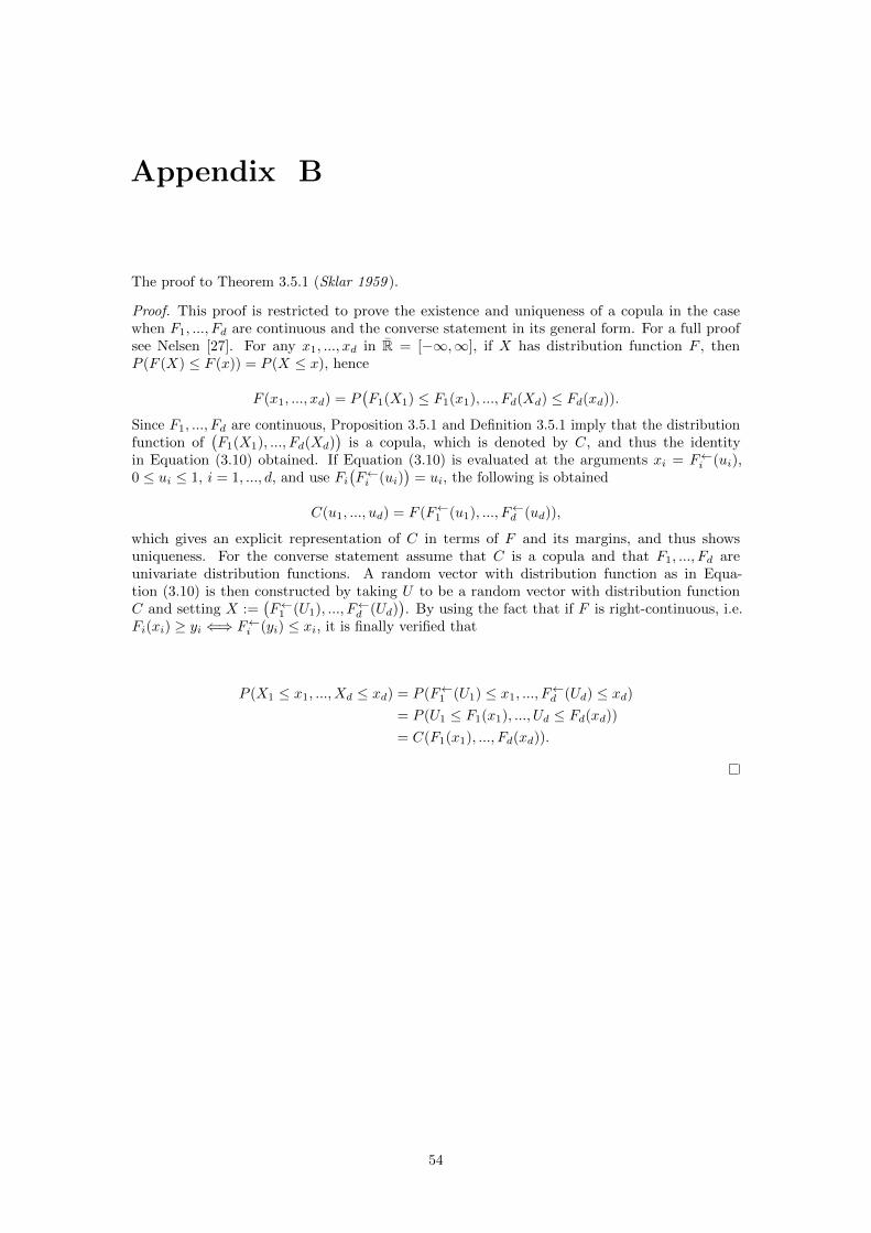
Appendix B
The proof to Theorem 3.5.1 (Sklar 1959 ).
Proof. This proof is restricted to prove the existence and uniqueness of a copula in the casewhen F1, ..., Fd are continuous and the converse statement in its general form. For a full proofsee Nelsen [27]. For any x1, ..., xd in R = [−∞,∞], if X has distribution function F , thenP (F (X) ≤ F (x)) = P (X ≤ x), hence
F (x1, ..., xd) = P(F1(X1) ≤ F1(x1), ..., Fd(Xd) ≤ Fd(xd)).
Since F1, ..., Fd are continuous, Proposition 3.5.1 and Definition 3.5.1 imply that the distributionfunction of
(F1(X1), ..., Fd(Xd)
)is a copula, which is denoted by C, and thus the identity
in Equation (3.10) obtained. If Equation (3.10) is evaluated at the arguments xi = F←i (ui),0 ≤ ui ≤ 1, i = 1, ..., d, and use Fi
(F←i (ui)
)= ui, the following is obtained
C(u1, ..., ud) = F (F←1 (u1), ..., F←d (ud)),
which gives an explicit representation of C in terms of F and its margins, and thus showsuniqueness. For the converse statement assume that C is a copula and that F1, ..., Fd areunivariate distribution functions. A random vector with distribution function as in Equa-tion (3.10) is then constructed by taking U to be a random vector with distribution functionC and setting X :=
(F←1 (U1), ..., F←d (Ud)
). By using the fact that if F is right-continuous, i.e.
Fi(xi) ≥ yi ⇐⇒ F←i (yi) ≤ xi, it is finally verified that
P (X1 ≤ x1, ..., Xd ≤ xd) = P (F←1 (U1) ≤ x1, ..., F←d (Ud) ≤ xd)
= P (U1 ≤ F1(x1), ..., Ud ≤ Fd(xd))= C(F1(x1), ..., Fd(xd)).
54

Appendix C
Proposition C.1. Let W(Y) denote the vector with ith component
Wi(Yi) = T−1ν
(Fi(Yi)
),
and let∣∣∂W∂Y
∣∣ denote the determinant of the Jacobian matrix associated with the transforma-tion (4.20). Then the conditional distribution on the raw variables is given by
fY(Y1|Y2) = fW(W1(Y1)|W2(Y2)
)∣∣∣∣∂W1
∂Y1
∣∣∣∣,where
∂W1
∂Y1(y1) =
f1(y1)
tν(T−1ν
(F1(y1)
)) .Given fY(Y1|Y2), it is easy to extract the conditional distribution for any particular component,say the jth component y1,j , of Y1, given Y2. The distribution of y1,j , given Y2, is then given by
fY(y1,j |Y2) = fW(w1,j(y1,j)|W2(Y2)
)∣∣∣∣∣ f1(y1,j)
tν(T−1ν
(F1(y1,j)
)) ∣∣∣∣∣For a full proof of Proposition C.1 please see [13] and [14].
55

Appendix D
In Table D.1-D.24 the values from the most volatile period in the out-of-sample set can beseen together with the conditional values and the corresponding estimated quantile values forα = {0.001, 0.005, 0.995, 0.999} for each method.
SR:normal, α = 0.999Nmiss = 0 Nmiss = 250
Date Monthly Yearly Yo−o−s Ypre |∆| ∆% Ypre |∆| ∆%2008-03-03 -7.9176 -2.4645 -10.3876 -3.2494 7.1382 0.6872 -3.5995 6.7881 0.65352008-02-29 -4.8392 0 -5.9767 -0.1792 5.7974 0.9700 -0.5358 5.4408 0.91032008-02-28 0.4615 0.3806 1.3294 2.9847 1.6553 -1.2451 2.4371 1.1077 -0.83332008-02-27 7.4380 2.5366 7.4603 8.0582 0.5979 -0.0801 7.3364 0.1239 0.01662008-02-26 -6.3467 -2.6591 -7.6246 -2.4807 5.1439 0.6746 -2.9017 4.7230 0.61942008-02-25 -7.7143 -0.5666 -8.2100 -2.0932 6.1168 0.7450 -2.3630 5.8469 0.7122
Table D.1: An overview of the values from the most volatile period in the out-of-sample set togetherwith the conditional values, and the corresponding estimated quantile values for α = 0.999 for theSR:normal method. The absolute error (distance) between the true value and the estimated value
together with the percentage error is also presented for two different scenarios.
SR:normal, α = 0.995Nmiss = 0 Nmiss = 250
Date Monthly Yearly Yo−o−s Ypre |∆| ∆% Ypre |∆| ∆%2008-03-03 -7.9176 -2.4645 -10.3876 -3.6627 6.7249 0.6474 -3.9248 6.4628 0.62222008-02-29 -4.8392 0 -5.9767 -0.5925 5.3841 0.9009 -0.8612 5.1155 0.85592008-02-28 0.4615 0.3806 1.3294 2.5713 1.2420 -0.9342 2.1118 0.7824 -0.58862008-02-27 7.4380 2.5366 7.4603 7.6449 0.1846 -0.0247 7.0111 0.4492 0.06022008-02-26 -6.3467 -2.6591 -7.6246 -2.8940 4.7306 0.6204 -3.2270 4.3976 0.57682008-02-25 -7.7143 -0.5666 -8.2100 -2.5065 5.7034 0.6947 -2.6883 5.5216 0.6726
Table D.2: An overview of the values from the most volatile period in the out-of-sample set togetherwith the conditional values, and the corresponding estimated quantile values for α = 0.995 for theSR:normal method. The absolute error (distance) between the true value and the estimated value
together with the percentage error is also presented for two different scenarios.
56

SR:normal, α = 0.005Nmiss = 0 Nmiss = 250
Date Monthly Yearly Yo−o−s Ypre |∆| ∆% Ypre |∆| ∆%2008-03-03 -7.9176 -2.4645 -10.3876 -7.8019 2.5857 0.2489 -7.1828 3.2048 0.30852008-02-29 -4.8392 0 -5.9767 -4.7318 1.2449 0.2083 -4.1191 1.8575 0.31082008-02-28 0.4615 0.3806 1.3294 -1.5679 2.8973 2.1794 -1.1462 2.4756 1.86222008-02-27 7.4380 2.5366 7.4603 3.5057 3.9546 0.5301 3.7531 3.7072 0.49692008-02-26 -6.3467 -2.6591 -7.6246 -7.0332 0.5914 0.0776 -6.4850 1.1397 0.14952008-02-25 -7.7143 -0.5666 -8.2100 -6.6457 1.5642 0.1905 -5.9463 2.2636 0.2757
Table D.3: An overview of the values from the most volatile period in the out-of-sample set togetherwith the conditional values, and the corresponding estimated quantile values for α = 0.005 for theSR:normal method. The absolute error (distance) between the true value and the estimated value
together with the percentage error is also presented for two different scenarios.
SR:normal, α = 0.001Nmiss = 0 Nmiss = 250
Date Monthly Yearly Yo−o−s Ypre |∆| ∆% Ypre |∆| ∆%2008-03-03 -7.9176 -2.4645 -10.3876 -8.2152 2.1724 0.2091 -7.5081 2.8795 0.27722008-02-29 -4.8392 0 -5.9767 -5.1451 0.8316 0.1391 -4.4445 1.5322 0.25642008-02-28 0.4615 0.3806 1.3294 -1.9812 3.3106 2.4903 -1.4715 2.8009 2.10692008-02-27 7.4380 2.5366 7.4603 3.0924 4.3679 0.5855 3.4278 4.0325 0.54052008-02-26 -6.3467 -2.6591 -7.6246 -7.4465 0.1781 0.0234 -6.8103 0.8143 0.10682008-02-25 -7.7143 -0.5666 -8.2100 -7.0591 1.1509 0.1402 -6.2716 1.9383 0.2361
Table D.4: An overview of the values from the most volatile period in the out-of-sample set togetherwith the conditional values, and the corresponding estimated quantile values for α = 0.001 for theSR:normal method. The absolute error (distance) between the true value and the estimated value
together with the percentage error is also presented for two different scenarios.
SR:Student’s t, α = 0.999Nmiss = 0 Nmiss = 250
Date Monthly Yearly Yo−o−s Ypre |∆| ∆% Ypre |∆| ∆%2008-03-03 -7.9176 -2.4645 -10.3876 -0.7847 9.6029 0.9245 -3.3557 7.0319 0.67692008-02-29 -4.8392 0 -5.9767 2.2813 8.2580 1.3817 -0.3007 5.6759 0.94972008-02-28 0.4615 0.3806 1.3294 5.5690 4.2396 -3.1891 2.7361 1.4067 -1.05812008-02-27 7.4380 2.5366 7.4603 10.7493 3.2890 -0.4409 7.6856 0.2253 -0.03022008-02-26 -6.3467 -2.6591 -7.6246 0.0311 7.6557 1.0041 -2.6327 4.9919 0.65472008-02-25 -7.7143 -0.5666 -8.2100 0.3125 8.5224 1.0381 -2.1552 6.0548 0.7375
Table D.5: An overview of the values from the most volatile period in the out-of-sample set togetherwith the conditional values, and the corresponding estimated quantile values for α = 0.999 for theSR:Student’s t method. The absolute error (distance) between the true value and the estimated value
together with the percentage error is also presented for two different scenarios.
57

SR:Student’s t, α = 0.995Nmiss = 0 Nmiss = 250
Date Monthly Yearly Yo−o−s Ypre |∆| ∆% Ypre |∆| ∆%2008-03-03 -7.9176 -2.4645 -10.3876 -2.9356 7.4520 0.7174 -3.8788 6.5088 0.62662008-02-29 -4.8392 0 -5.9767 0.1304 6.1071 1.0218 -0.8238 5.1529 0.86222008-02-28 0.4615 0.3806 1.3294 3.4181 2.0887 -1.5712 2.2130 0.8836 -0.66472008-02-27 7.4380 2.5366 7.4603 8.5984 1.1381 -0.1526 7.1626 0.2978 0.03992008-02-26 -6.3467 -2.6591 -7.6246 -2.1198 5.5048 0.7220 -3.1558 4.4688 0.58612008-02-25 -7.7143 -0.5666 -8.2100 -1.8384 6.3715 0.7761 -2.6783 5.5317 0.6738
Table D.6: An overview of the values from the most volatile period in the out-of-sample set togetherwith the conditional values, and the corresponding estimated quantile values for α = 0.995 for theSR:Student’s t method. The absolute error (distance) between the true value and the estimated value
together with the percentage error is also presented for two different scenarios.
SR:Student’s t, α = 0.005Nmiss = 0 Nmiss = 250
Date Monthly Yearly Yo−o−s Ypre |∆| ∆% Ypre |∆| ∆%2008-03-03 -7.9176 -2.4645 -10.3876 -8.8089 1.5787 0.1520 -7.3425 3.0451 0.29312008-02-29 -4.8392 0 -5.9767 -5.7428 0.2338 0.0391 -4.2875 1.6891 0.28262008-02-28 0.4615 0.3806 1.3294 -2.4552 3.7846 2.8469 -1.2507 2.5801 1.94082008-02-27 7.4380 2.5366 7.4603 2.7251 4.7352 0.6347 3.6989 3.7615 0.50422008-02-26 -6.3467 -2.6591 -7.6246 -7.9931 0.3684 -0.0483 -6.6195 1.0051 0.13182008-02-25 -7.7143 -0.5666 -8.2100 -7.7117 0.4982 0.0607 -6.1420 2.0680 0.2519
Table D.7: An overview of the values from the most volatile period in the out-of-sample set togetherwith the conditional values, and the corresponding estimated quantile values for α = 0.005 for theSR:Student’s t method. The absolute error (distance) between the true value and the estimated value
together with the percentage error is also presented for two different scenarios.
SR:Student’s t, α = 0.001Nmiss = 0 Nmiss = 250
Date Monthly Yearly Yo−o−s Ypre |∆| ∆% Ypre |∆| ∆%2008-03-03 -7.9176 -2.4645 -10.3876 -10.9598 0.5722 -0.0551 -7.8656 2.5220 0.24282008-02-29 -4.8392 0 -5.9767 -7.8937 1.9171 -0.3208 -4.8106 1.1661 0.19512008-02-28 0.4615 0.3806 1.3294 -4.6061 5.9355 4.4648 -1.7738 3.1032 2.33432008-02-27 7.4380 2.5366 7.4603 0.5742 6.8861 0.9230 3.1758 4.2845 0.57432008-02-26 -6.3467 -2.6591 -7.6246 -10.1440 2.5193 -0.3304 -7.1426 0.4820 0.06322008-02-25 -7.7143 -0.5666 -8.2100 -9.8626 1.6527 -0.2013 -6.6651 1.5449 0.1882
Table D.8: An overview of the values from the most volatile period in the out-of-sample set togetherwith the conditional values, and the corresponding estimated quantile values for α = 0.001 for theSR:Student’s t method. The absolute error (distance) between the true value and the estimated value
together with the percentage error is also presented for two different scenarios.
58

MI:normal, α = 0.999Nmiss = 0 Nmiss = 250
Date Monthly Yearly Yo−o−s Ypre |∆| ∆% Ypre |∆| ∆%2008-03-03 -7.9176 -2.4645 -10.3876 -3.2495 7.1381 0.6872 -3.5800 6.8076 0.65542008-02-29 -4.8392 0 -5.9767 -0.1810 5.7957 0.9697 -0.5149 5.4618 0.91392008-02-28 0.4615 0.3806 1.3294 2.9865 1.6571 -1.2465 2.4420 1.1126 -0.83692008-02-27 7.4380 2.5366 7.4603 8.0620 0.6017 -0.0807 7.3281 0.1322 0.01772008-02-26 -6.3467 -2.6591 -7.6246 -2.4792 5.1455 0.6748 -2.8884 4.7362 0.62122008-02-25 -7.7143 -0.5666 -8.2100 -2.0963 6.1137 0.7447 -2.3351 5.8749 0.7156
Table D.9: An overview of the values from the most volatile period in the out-of-sample set togetherwith the conditional values, and the corresponding estimated quantile values for α = 0.999 for theMI:normal method. The absolute error (distance) between the true value and the estimated value
together with the percentage error is also presented for two different scenarios.
MI:normal, α = 0.995Nmiss = 0 Nmiss = 250
Date Monthly Yearly Yo−o−s Ypre |∆| ∆% Ypre |∆| ∆%2008-03-03 -7.9176 -2.4645 -10.3876 -3.6621 6.7255 0.6475 -3.8955 6.4921 0.62502008-02-29 -4.8392 0 -5.9767 -0.5880 5.3886 0.9016 -0.8298 5.1469 0.86122008-02-28 0.4615 0.3806 1.3294 2.5753 1.2459 -0.9372 2.1213 0.7919 -0.59572008-02-27 7.4380 2.5366 7.4603 7.6512 0.1909 -0.0256 7.0026 0.4577 0.06132008-02-26 -6.3467 -2.6591 -7.6246 -2.8942 4.7304 0.6204 -3.2063 4.4184 0.57952008-02-25 -7.7143 -0.5666 -8.2100 -2.5024 5.7076 0.6952 -2.6474 5.5625 0.6775
Table D.10: An overview of the values from the most volatile period in the out-of-sample set togetherwith the conditional values, and the corresponding estimated quantile values for α = 0.995 for theMI:normal method. The absolute error (distance) between the true value and the estimated value
together with the percentage error is also presented for two different scenarios.
MI:normal, α = 0.005Nmiss = 0 Nmiss = 250
Date Monthly Yearly Yo−o−s Ypre |∆| ∆% Ypre |∆| ∆%2008-03-03 -7.9176 -2.4645 -10.3876 -7.8047 2.5829 0.2487 -7.1525 3.2351 0.31142008-02-29 -4.8392 0 -5.9767 -4.7424 1.2343 0.2065 -4.0895 1.8872 0.31582008-02-28 0.4615 0.3806 1.3294 -1.5728 2.9022 2.1831 -1.1354 2.4648 1.85412008-02-27 7.4380 2.5366 7.4603 3.5000 3.9603 0.5308 3.7466 3.7137 0.49782008-02-26 -6.3467 -2.6591 -7.6246 -7.0328 0.5918 0.0776 -6.4617 1.1629 0.15252008-02-25 -7.7143 -0.5666 -8.2100 -6.6576 1.5524 0.1891 -5.9080 2.3020 0.2804
Table D.11: An overview of the values from the most volatile period in the out-of-sample set togetherwith the conditional values, and the corresponding estimated quantile values for α = 0.005 for theMI:normal method. The absolute error (distance) between the true value and the estimated value
together with the percentage error is also presented for two different scenarios.
59

MI:normal, α = 0.001Nmiss = 0 Nmiss = 250
Date Monthly Yearly Yo−o−s Ypre |∆| ∆% Ypre |∆| ∆%2008-03-03 -7.9176 -2.4645 -10.3876 -8.2223 2.1652 0.2084 -7.4848 2.9028 0.27942008-02-29 -4.8392 0 -5.9767 -5.1545 0.8222 0.1376 -4.4170 1.5597 0.26102008-02-28 0.4615 0.3806 1.3294 -1.9843 3.3137 2.4927 -1.4638 2.7932 2.10112008-02-27 7.4380 2.5366 7.4603 3.0931 4.3672 0.5854 3.4210 4.0393 0.54142008-02-26 -6.3467 -2.6591 -7.6246 -7.4510 0.1737 0.0228 -6.7950 0.8296 0.10882008-02-25 -7.7143 -0.5666 -8.2100 -7.0709 1.1390 0.1387 -6.2359 1.9740 0.2404
Table D.12: An overview of the values from the most volatile period in the out-of-sample set togetherwith the conditional values, and the corresponding estimated quantile values for α = 0.001 for theMI:normal method. The absolute error (distance) between the true value and the estimated value
together with the percentage error is also presented for two different scenarios.
MI:Student’s t, α = 0.999Nmiss = 0 Nmiss = 250
Date Monthly Yearly Yo−o−s Ypre |∆| ∆% Ypre |∆| ∆%2008-03-03 -7.9176 -2.4645 -10.3876 -0.7908 9.5968 0.9239 -3.3153 7.0723 0.68082008-02-29 -4.8392 0 -5.9767 2.2760 8.2527 1.3808 -0.3314 5.6452 0.94452008-02-28 0.4615 0.3806 1.3294 5.5668 4.2374 -3.1875 2.7279 1.3985 -1.05202008-02-27 7.4380 2.5366 7.4603 3.0931 4.3672 0.5854 3.4210 4.0393 0.54142008-02-26 -6.3467 -2.6591 -7.6246 0.0261 7.6507 1.0034 -2.5741 5.0505 0.66242008-02-25 -7.7143 -0.5666 -8.2100 0.3056 8.5155 1.0372 -2.1846 6.0254 0.7339
Table D.13: An overview of the values from the most volatile period in the out-of-sample set togetherwith the conditional values, and the corresponding estimated quantile values for α = 0.999 for theMI:Student’s t method. The absolute error (distance) between the true value and the estimated value
together with the percentage error is also presented for two different scenarios.
MI:Student’s t, α = 0.995Nmiss = 0 Nmiss = 250
Date Monthly Yearly Yo−o−s Ypre |∆| ∆% Ypre |∆| ∆%2008-03-03 -7.9176 -2.4645 -10.3876 -2.9315 7.4561 0.7178 -3.8397 6.5479 0.63042008-02-29 -4.8392 0 -5.9767 0.1342 6.1108 1.0224 -0.8546 5.1221 0.85702008-02-28 0.4615 0.3806 1.3294 3.4165 2.0871 -1.5700 2.1993 0.8699 -0.65432008-02-27 7.4380 2.5366 7.4603 8.5919 1.1316 -0.1517 7.1124 0.3479 0.04662008-02-26 -6.3467 -2.6591 -7.6246 -2.1177 5.5070 0.7223 -3.1008 4.5239 0.59332008-02-25 -7.7143 -0.5666 -8.2100 -1.8323 6.3777 0.7768 -2.7055 5.5044 0.6705
Table D.14: An overview of the values from the most volatile period in the out-of-sample set togetherwith the conditional values, and the corresponding estimated quantile values for α = 0.995 for theMI:Student’s t method. The absolute error (distance) between the true value and the estimated value
together with the percentage error is also presented for two different scenarios.
60
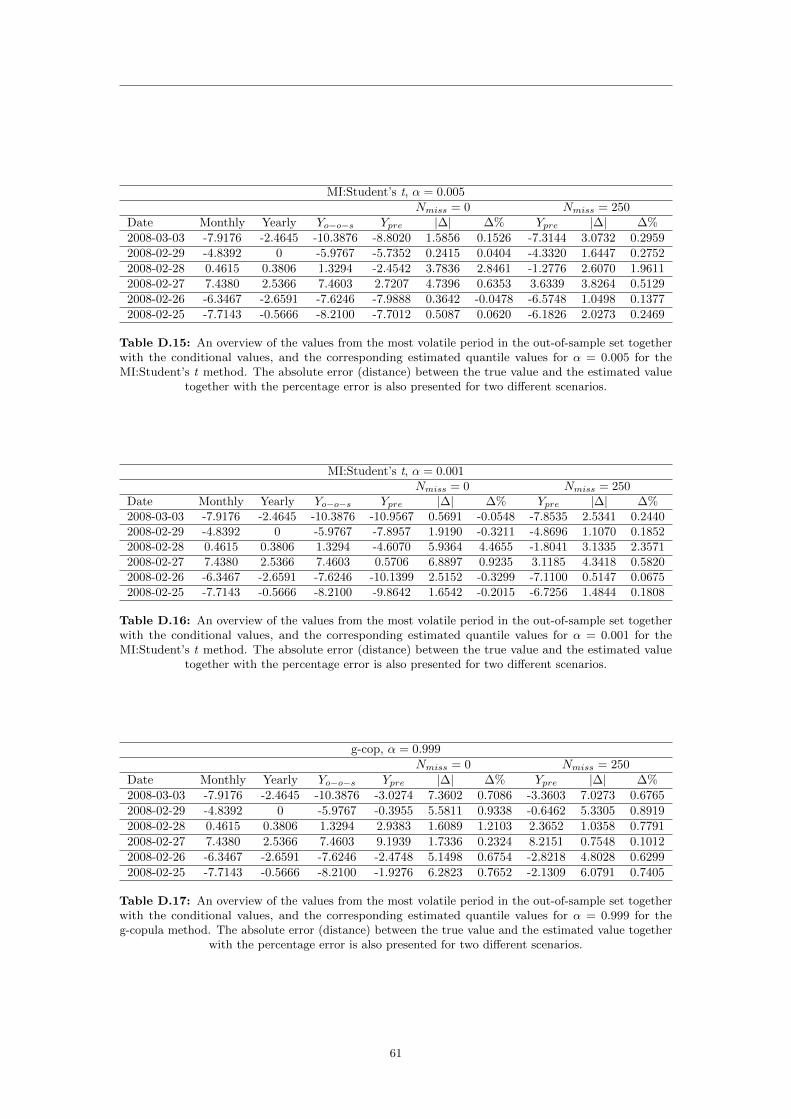
MI:Student’s t, α = 0.005Nmiss = 0 Nmiss = 250
Date Monthly Yearly Yo−o−s Ypre |∆| ∆% Ypre |∆| ∆%2008-03-03 -7.9176 -2.4645 -10.3876 -8.8020 1.5856 0.1526 -7.3144 3.0732 0.29592008-02-29 -4.8392 0 -5.9767 -5.7352 0.2415 0.0404 -4.3320 1.6447 0.27522008-02-28 0.4615 0.3806 1.3294 -2.4542 3.7836 2.8461 -1.2776 2.6070 1.96112008-02-27 7.4380 2.5366 7.4603 2.7207 4.7396 0.6353 3.6339 3.8264 0.51292008-02-26 -6.3467 -2.6591 -7.6246 -7.9888 0.3642 -0.0478 -6.5748 1.0498 0.13772008-02-25 -7.7143 -0.5666 -8.2100 -7.7012 0.5087 0.0620 -6.1826 2.0273 0.2469
Table D.15: An overview of the values from the most volatile period in the out-of-sample set togetherwith the conditional values, and the corresponding estimated quantile values for α = 0.005 for theMI:Student’s t method. The absolute error (distance) between the true value and the estimated value
together with the percentage error is also presented for two different scenarios.
MI:Student’s t, α = 0.001Nmiss = 0 Nmiss = 250
Date Monthly Yearly Yo−o−s Ypre |∆| ∆% Ypre |∆| ∆%2008-03-03 -7.9176 -2.4645 -10.3876 -10.9567 0.5691 -0.0548 -7.8535 2.5341 0.24402008-02-29 -4.8392 0 -5.9767 -7.8957 1.9190 -0.3211 -4.8696 1.1070 0.18522008-02-28 0.4615 0.3806 1.3294 -4.6070 5.9364 4.4655 -1.8041 3.1335 2.35712008-02-27 7.4380 2.5366 7.4603 0.5706 6.8897 0.9235 3.1185 4.3418 0.58202008-02-26 -6.3467 -2.6591 -7.6246 -10.1399 2.5152 -0.3299 -7.1100 0.5147 0.06752008-02-25 -7.7143 -0.5666 -8.2100 -9.8642 1.6542 -0.2015 -6.7256 1.4844 0.1808
Table D.16: An overview of the values from the most volatile period in the out-of-sample set togetherwith the conditional values, and the corresponding estimated quantile values for α = 0.001 for theMI:Student’s t method. The absolute error (distance) between the true value and the estimated value
together with the percentage error is also presented for two different scenarios.
g-cop, α = 0.999Nmiss = 0 Nmiss = 250
Date Monthly Yearly Yo−o−s Ypre |∆| ∆% Ypre |∆| ∆%2008-03-03 -7.9176 -2.4645 -10.3876 -3.0274 7.3602 0.7086 -3.3603 7.0273 0.67652008-02-29 -4.8392 0 -5.9767 -0.3955 5.5811 0.9338 -0.6462 5.3305 0.89192008-02-28 0.4615 0.3806 1.3294 2.9383 1.6089 1.2103 2.3652 1.0358 0.77912008-02-27 7.4380 2.5366 7.4603 9.1939 1.7336 0.2324 8.2151 0.7548 0.10122008-02-26 -6.3467 -2.6591 -7.6246 -2.4748 5.1498 0.6754 -2.8218 4.8028 0.62992008-02-25 -7.7143 -0.5666 -8.2100 -1.9276 6.2823 0.7652 -2.1309 6.0791 0.7405
Table D.17: An overview of the values from the most volatile period in the out-of-sample set togetherwith the conditional values, and the corresponding estimated quantile values for α = 0.999 for theg-copula method. The absolute error (distance) between the true value and the estimated value together
with the percentage error is also presented for two different scenarios.
61

g-cop, α = 0.995Nmiss = 0 Nmiss = 250
Date Monthly Yearly Yo−o−s Ypre |∆| ∆% Ypre |∆| ∆%2008-03-03 -7.9176 -2.4645 -10.3876 -3.4290 6.9586 0.6699 -3.7541 6.6335 0.63862008-02-29 -4.8392 0 -5.9767 -0.7563 5.2204 0.8735 -0.9942 4.9825 0.83372008-02-28 0.4615 0.3806 1.3294 2.5219 1.1925 0.8970 2.0280 0.6986 0.52552008-02-27 7.4380 2.5366 7.4603 8.4985 1.0382 0.1392 7.6473 0.1870 0.02512008-02-26 -6.3467 -2.6591 -7.6246 -2.8642 4.7604 0.6243 -3.1820 4.4427 0.58272008-02-25 -7.7143 -0.5666 -8.2100 -2.3016 5.9083 0.7197 -2.5178 5.6922 0.6933
Table D.18: An overview of the values from the most volatile period in the out-of-sample set togetherwith the conditional values, and the corresponding estimated quantile values for α = 0.995 for theg-copula method. The absolute error (distance) between the true value and the estimated value together
with the percentage error is also presented for two different scenarios.
g-cop, α = 0.005Nmiss = 0 Nmiss = 250
Date Monthly Yearly Yo−o−s Ypre |∆| ∆% Ypre |∆| ∆%2008-03-03 -7.9176 -2.4645 -10.3876 -8.6685 1.7191 0.1655 -8.2964 2.0912 0.20132008-02-29 -4.8392 0 -5.9767 -4.8883 1.0884 0.1821 -4.3007 1.6760 0.28042008-02-28 0.4615 0.3806 1.3294 -1.3326 2.6619 2.0024 -0.9202 2.2496 1.69222008-02-27 7.4380 2.5366 7.4603 3.1298 4.3305 0.5805 3.3406 4.1197 0.55222008-02-26 -6.3467 -2.6591 -7.6246 -7.7988 0.1741 0.0228 -7.4075 0.2171 0.0282008-02-25 -7.7143 -0.5666 -8.2100 -6.9938 1.2161 0.1481 -6.4244 1.7856 0.2175
Table D.19: An overview of the values from the most volatile period in the out-of-sample set togetherwith the conditional values, and the corresponding estimated quantile values for α = 0.005 for theg-copula method. The absolute error (distance) between the true value and the estimated value together
with the percentage error is also presented for two different scenarios.
g-cop, α = 0.001Nmiss = 0 Nmiss = 250
Date Monthly Yearly Yo−o−s Ypre |∆| ∆% Ypre |∆| ∆%2008-03-03 -7.9176 -2.4645 -10.3876 -9.2252 1.1624 0.1119 -8.7791 1.6085 0.15492008-02-29 -4.8392 0 -5.9767 -5.3029 0.6737 0.1127 -4.6234 1.3532 0.22642008-02-28 0.4615 0.3806 1.3294 -1.6993 3.0287 2.2783 -1.1991 2.5285 1.90202008-02-27 7.4380 2.5366 7.4603 2.6755 4.7849 0.6414 2.9850 4.4753 0.59992008-02-26 -6.3467 -2.6591 -7.6246 -8.3305 0.7058 0.0926 -7.8680 0.2433 0.03192008-02-25 -7.7143 -0.5666 -8.2100 -7.4705 0.7395 0.0901 -6.8082 1.4017 0.1707
Table D.20: An overview of the values from the most volatile period in the out-of-sample set togetherwith the conditional values, and the corresponding estimated quantile values for α = 0.001 for theg-copula method. The absolute error (distance) between the true value and the estimated value together
with the percentage error is also presented for two different scenarios.
62

t-cop, α = 0.999Nmiss = 0 Nmiss = 250
Date Monthly Yearly Yo−o−s Ypre |∆| ∆% Ypre |∆| ∆%2008-03-03 -7.9176 -2.4645 -10.3876 -3.4317 6.9559 0.6696 -2.0144 8.3732 0.80612008-02-29 -4.8392 0 -5.9767 -0.5387 5.4379 0.9099 0.8110 6.7877 1.13572008-02-28 0.4615 0.3806 1.3294 2.3205 0.9911 0.7455 3.1877 1.8583 1.39782008-02-27 7.4380 2.5366 7.4603 7.4587 0.0016 0.0002 7.6590 0.1987 0.02662008-02-26 -6.3467 -2.6591 -7.6246 -2.8736 4.7510 0.6231 -1.5943 6.0303 0.79092008-02-25 -7.7143 -0.5666 -8.2100 -2.1065 6.1035 0.7434 -0.4631 7.7468 0.9436
Table D.21: An overview of the values from the most volatile period in the out-of-sample set togetherwith the conditional values, and the corresponding estimated quantile values for α = 0.999 for thet-copula method. The absolute error (distance) between the true value and the estimated value together
with the percentage error is also presented for two different scenarios.
t-cop, α = 0.995Nmiss = 0 Nmiss = 250
Date Monthly Yearly Yo−o−s Ypre |∆| ∆% Ypre |∆| ∆%2008-03-03 -7.9176 -2.4645 -10.3876 -4.0660 6.3216 0.6086 -2.9376 7.4500 0.71722008-02-29 -4.8392 0 -5.9767 -1.1605 4.8162 0.8058 -0.0045 5.9722 0.99922008-02-28 0.4615 0.3806 1.3294 1.8980 0.5686 0.4277 2.5748 1.2454 0.93692008-02-27 7.4380 2.5366 7.4603 7.0302 0.4301 0.0577 7.0842 0.3761 0.05042008-02-26 -6.3467 -2.6591 -7.6246 -3.4305 4.1942 0.5501 -2.4498 5.1748 0.67872008-02-25 -7.7143 -0.5666 -8.2100 -2.8775 5.3325 0.6495 -1.4824 6.7275 0.8194
Table D.22: An overview of the values from the most volatile period in the out-of-sample set togetherwith the conditional values, and the corresponding estimated quantile values for α = 0.995 for thet-copula method. The absolute error (distance) between the true value and the estimated value together
with the percentage error is also presented for two different scenarios.
t-cop, α = 0.005Nmiss = 0 Nmiss = 250
Date Monthly Yearly Yo−o−s Ypre |∆| ∆% Ypre |∆| ∆%2008-03-03 -7.9176 -2.4645 -10.3876 -7.2424 3.1452 0.3028 -7.5755 2.8121 0.27072008-02-29 -4.8392 0 -5.9767 -4.5235 1.4531 0.2431 -4.9661 1.0106 0.16912008-02-28 0.4615 0.3806 1.3294 -0.8312 2.1605 1.6252 -1.4892 2.8186 2.12022008-02-27 7.4380 2.5366 7.4603 3.7367 3.7236 0.4991 2.7895 4.6708 0.62612008-02-26 -6.3467 -2.6591 -7.6246 -6.3278 1.2969 0.1701 -6.7285 0.8962 0.11752008-02-25 -7.7143 -0.5666 -8.2100 -6.6755 1.5345 0.1869 -7.0169 1.1930 0.1453
Table D.23: An overview of the values from the most volatile period in the out-of-sample set togetherwith the conditional values, and the corresponding estimated quantile values for α = 0.005 for thet-copula method. The absolute error (distance) between the true value and the estimated value together
with the percentage error is also presented for two different scenarios.
63

t-cop, α = 0.001Nmiss = 0 Nmiss = 250
Date Monthly Yearly Yo−o−s Ypre |∆| ∆% Ypre |∆| ∆%2008-03-03 -7.9176 -2.4645 -10.3876 -7.7172 2.6704 0.2571 -8.1221 2.2655 0.21812008-02-29 -4.8392 0 -5.9767 -5.0440 0.9326 0.1560 -5.6073 0.3694 0.06182008-02-28 0.4615 0.3806 1.3294 -1.3195 2.6489 1.9926 -2.1577 3.4871 2.62312008-02-27 7.4380 2.5366 7.4603 3.0303 4.4300 0.5938 1.8021 5.6582 0.75842008-02-26 -6.3467 -2.6591 -7.6246 -6.7714 0.8532 0.1119 -7.2429 0.3817 0.05012008-02-25 -7.7143 -0.5666 -8.2100 -7.2278 0.9822 0.1196 -7.6668 0.5432 0.0662
Table D.24: An overview of the values from the most volatile period in the out-of-sample set togetherwith the conditional values, and the corresponding estimated quantile values for α = 0.001 for thet-copula method. The absolute error (distance) between the true value and the estimated value together
with the percentage error is also presented for two different scenarios.
64

Appendix E
In Figure E.1-E.2 and in Table E.1-E.2 the calculated MAE and RMSE for each method canbe seen when the models are applied on more stable data. Since the MAE and the RMSE iscalculated after generating predicted values from the corresponding conditional distribution, andboth is very sensitive when used on small samples (typically Nmiss < 100), these error metricshave been averaged over 100 iterations for a more distinguishable interpretation.
Number of Missing Values0 50 100 150 200 250
MeanAbsolute
Error
0.3
0.35
0.4
0.45
0.5
0.55
0.6
0.65
0.7
0.75
0.8
SR:Normal
SR:Students t
MI:Normal
MI:Students t
g-cop
t-cop
Figure E.1: The Mean Absolute Error (MAE) for each model with different amount of missingdata (NaN).
Mean Absolute Error (MAE)NaN 3 10 25 50 100 150 250SR:normal 0.6475 0.6310 0.6675 0.6954 0.6846 0.7243 0.7632SR:Student’s t 0.6337 0.5828 0.5643 0.6336 0.6056 0.6593 0.6763MI:normal 0.6264 0.6331 0.6486 0.6891 0.6851 0.7289 0.7612MI:Student’s t 0.6479 0.5743 0.5479 0.6178 0.6081 0.6651 0.6802g-cop 0.5588 0.5613 0.5736 0.6343 0.6211 0.6635 0.7033t-cop 0.4169 0.3306 0.3600 0.4425 0.4588 0.5803 0.5695
Table E.1: The Mean Absolute Error (MAE) for each model with different amount of missing data (NaN).
65

Number of Missing Values0 50 100 150 200 250
RootMeanSquare
Error
0.4
0.5
0.6
0.7
0.8
0.9
1
SR:Normal
SR:Students t
MI:Normal
MI:Students t
g-cop
t-cop
Figure E.2: The Root Mean Square Error (RMSE) for each model with different amount of missingdata (NaN).
Root Mean Square Error (RMSE)NaN 3 10 25 50 100 150 250SR:normal 0.7517 0.7667 0.8150 0.8749 0.8592 0.9126 0.9613SR:Student’s t 0.7583 0.8166 0.8023 0.9380 0.8611 0.9410 0.9257MI:normal 0.7148 0.7724 0.8035 0.8634 0.8600 0.9181 0.9586MI:Student’s t 0.7673 0.7749 0.7646 0.8768 0.8740 0.9410 0.9337g-cop 0.6504 0.6925 0.7138 0.8142 0.7911 0.8514 0.8927t-cop 0.4893 0.4144 0.4655 0.5915 0.6028 0.7622 0.7428
Table E.2: The Root Mean Square Error (RMSE) for each model with different amount of missingdata (NaN).
66
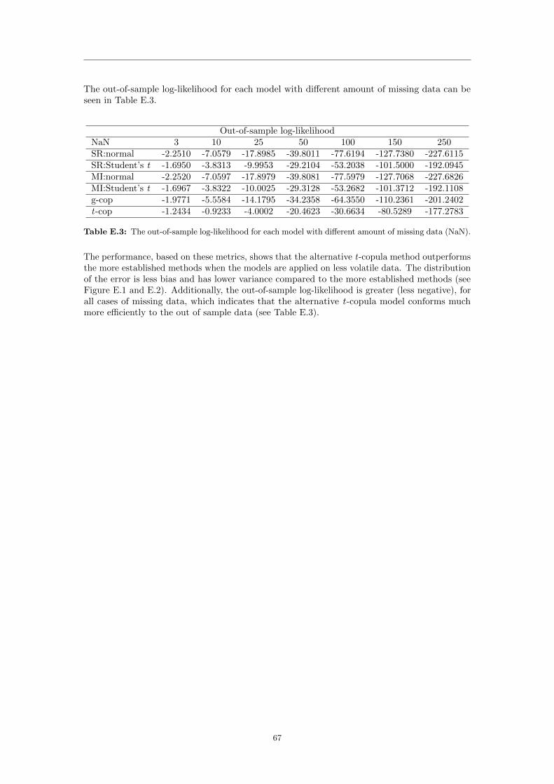
The out-of-sample log-likelihood for each model with different amount of missing data can beseen in Table E.3.
Out-of-sample log-likelihoodNaN 3 10 25 50 100 150 250SR:normal -2.2510 -7.0579 -17.8985 -39.8011 -77.6194 -127.7380 -227.6115SR:Student’s t -1.6950 -3.8313 -9.9953 -29.2104 -53.2038 -101.5000 -192.0945MI:normal -2.2520 -7.0597 -17.8979 -39.8081 -77.5979 -127.7068 -227.6826MI:Student’s t -1.6967 -3.8322 -10.0025 -29.3128 -53.2682 -101.3712 -192.1108g-cop -1.9771 -5.5584 -14.1795 -34.2358 -64.3550 -110.2361 -201.2402t-cop -1.2434 -0.9233 -4.0002 -20.4623 -30.6634 -80.5289 -177.2783
Table E.3: The out-of-sample log-likelihood for each model with different amount of missing data (NaN).
The performance, based on these metrics, shows that the alternative t-copula method outperformsthe more established methods when the models are applied on less volatile data. The distributionof the error is less bias and has lower variance compared to the more established methods (seeFigure E.1 and E.2). Additionally, the out-of-sample log-likelihood is greater (less negative), forall cases of missing data, which indicates that the alternative t-copula model conforms muchmore efficiently to the out of sample data (see Table E.3).
67