Rovib

Studying the Oscillation of Hydrochloric Acid via Gas Phase Vibrational-Rotational Infrared

Spectroscopy

Josiah Matthew

Bob Jones University Chemistry Department

1700 Wade Hampton BLVD

Greenville, SC 29614

Abstract

The following experiment studies the oscillations of hydrochloric acid using vibrational

rotational infrared spectroscopy. The spectral data is fitted to a polynomial from which the

moment of inertia and inter-nuclear distance are both calculated. These data can be used to

analyze how well an anharmonic oscillator fits our data. Most of the data corresponds well to

literature data, except for values predicted for an anharmonic oscillator. This suggest that HCl

best fits the model of a harmonic oscillator rigid rotor, and demonstrates very little

anharmonicity.

Introduction

The purpose of this experiment is to

study the harmonic and anharmonic

oscillations of HCl. A quantum harmonic

oscillator is a quantum mechanical

approximation of a classical harmonic

oscillator which follows Hook’s law. In this

model, a chemical bond is treated like a

spring, where a restoring force acts upon a

molecule when it is displaced from

equilibrium. A harmonic oscillating

molecule is quantized and only has

specifically allowed energy levels. The

simplest model of a harmonic oscillator is

the rigid rotor, which assumes that atoms

are joined by a rigid weightless rod which

does not distort under rotational stress. A

chemical bond is not truly rigid and

therefore does stretch some when rotated.

Anharmonicity is a deviation from

harmonicity where the actual potential is

different from the harmonic potential and

the actual vibrational energy levels are not

as predicted by harmonic oscillation due to

centrifugal distortion. This experiment uses

vibrational-rotational infrared spectroscopy

to determine study the harmonic-oscillator

rigid rotor model as it applies to HCl gas.

Infrared rotational-vibrational

(rovibrational) spectroscopy is used

extensively in physical chemistry. The

rovibrational spectra of polycyclic aromatic

hydrocarbons (PAHs) have been studied

and PAHs are thought to be responsible for

some of the unidentified spectral bands in

interstellar emissions1. One study that is

similar to this current experiment uses

rovibrational spectroscopy on various

isotopologues of carbon monoxide in order

to test molecular rotor theories by

calculating rotational constants and

predicting the center of mass and center of

interaction of the molecule2. Rovibrational

spectroscopy has been important in

determining the structural properties,

reaction kinetics, and dynamics of radicals

such as the phenyl radical, which has a

variety of uses due to its high reactivity, and

is considered the most important aromatic

radical in all of chemistry3. In addition,

rovibrational spectroscopy has been used in

determining the presence of

dichlorodifluoromethane (CFC-12), a

significant greenhouse gas, in the

atmosphere4. The chemical and physical

properties of SiO have also been discovered

using rovibrational spectroscopy, and this

data is important to its role in interstellar

space5.

This experiment uses a gas phase

infrared rovibrational spectrum to

determine the harmonic properties of HCl

gas. Because chlorine exists in isotopes 35Cl

(~75 %) and 37Cl (~25 %), two resolved

features are observed for each absorption

peak. The spectrum shows absorbances for

vibrational transitions following the

selection rule for a change in value of the

rotational quantum number of ∆𝐽 = ±1.

The spectrum is divided into R and P

branches, where ∆𝐽 = 1 for the R branch,

and ∆𝐽 = −1 for the P branch. This

experiment is concerned with transitions

from the ground state J’’ values to the first

excited state J’. The quantity m is defined as

𝑚 = 𝐽′′ + 1 for the R branch, and 𝑚 = −𝐽′′

for the P branch. The spectrum acquired in

this experiment is labelled with m and J’’

values. The wavenumber of absorbance, ��,

is plotted vs. the m value it represents. This

plot can be fit to a second order polynomial

in order to determine the following values

from equation 1:6

𝜈0 =

𝑡ℎ𝑒 𝑓𝑟𝑒𝑞𝑢𝑒𝑛𝑐𝑦 𝑜𝑓 𝑓𝑜𝑟𝑏𝑖𝑑𝑑𝑒𝑛 𝑡𝑟𝑎𝑛𝑠𝑖𝑡𝑖𝑜𝑛 (∆𝐽 =

0), 𝐵𝑒 =

𝑡ℎ𝑒 𝑟𝑜𝑡𝑎𝑡𝑖𝑜𝑛𝑎𝑙 𝑐𝑜𝑛𝑠𝑡𝑎𝑛𝑡, 𝑎𝑛𝑑 𝛼𝑒 =

𝑡ℎ𝑒 𝑣𝑖𝑏𝑟𝑎𝑡𝑖𝑜𝑛 −

𝑟𝑜𝑡𝑎𝑡𝑖𝑜𝑛 𝑖𝑛𝑡𝑒𝑟𝑎𝑐𝑡𝑖𝑜𝑛 𝑐𝑜𝑛𝑠𝑡𝑎𝑛𝑡.

��(𝑚) = 𝜈0 + (2𝐵𝑒 − 2𝛼𝑒)𝑚 − 𝛼𝑒𝑚2 (1)

This data can also be fit to a third order

polynomial6 in order to include a correction

for anharmonicity due to centrifugal

stretching,

𝐷𝑒 =

𝑡ℎ𝑒 𝑐𝑒𝑛𝑡𝑟𝑖𝑓𝑢𝑔𝑎𝑙 𝑑𝑖𝑠𝑡𝑜𝑟𝑡𝑖𝑜𝑛 𝑐𝑜𝑛𝑠𝑡𝑎𝑛𝑡.

��(𝑚) = 𝜈0 + (2𝐵𝑒 − 2𝛼𝑒)𝑚 − 𝛼𝑒𝑚2 −

4𝐷𝑒𝑚3 (2)

Once 𝐵𝑒 is known, the moment of inertia 𝐼𝑒

can be calculated using equation 3

(ℎ = 𝑝𝑙𝑎𝑛𝑐𝑘′𝑠 𝑐𝑜𝑛𝑠𝑡𝑎𝑛𝑡, 𝑐 =

𝑠𝑝𝑒𝑒𝑑 𝑜𝑓 𝑙𝑖𝑔ℎ𝑡).6

𝐼𝑒 =ℎ

8𝜋2𝐵𝑒𝑐 (3)

This is then used in equation 4 to calculate

the inter-nuclear distance, 𝑟𝑒:6

𝑟𝑒 = √𝐼

𝜇 (4)

where 𝜇 =𝑚1𝑚2

𝑚1+𝑚2 is the reduced mass. The

values for

𝜈�� =

𝑡ℎ𝑒 𝑓𝑢𝑛𝑑𝑎𝑚𝑒𝑛𝑡𝑎𝑙 𝑓𝑟𝑒𝑞𝑢𝑒𝑛𝑐𝑦 𝑜𝑓 𝑣𝑖𝑏𝑟𝑎𝑡𝑖𝑜𝑛

, and

𝜈��𝜒𝑒 = 𝑡ℎ𝑒 𝑎𝑛ℎ𝑎𝑟𝑚𝑜𝑛𝑖𝑐𝑖𝑡𝑦 𝑐𝑜𝑛𝑠𝑡𝑎𝑛𝑡 can

be determined by simultaneously solving

equations 5 and 6.6

𝜈0 = 𝜈�� − 2𝜈��𝜒𝑒 (5)

𝜈0∗ = 𝜈�� (

𝜇

𝜇∗)

1

2 − 2𝜈��𝜒𝑒

𝜇

𝜇∗ (6)

According to the rigid rotor prediction the

following equation6 is true:

𝐵𝑒∗

𝐵𝑒=

𝜇

𝜇∗ (7)

Therefore by calculating 𝐵𝑒

∗

𝐵𝑒, this will tell us

how close our data follows the rigid rotor

model.

Our results correspond well to

literature values, except for our values of

𝜈��and 𝜈��𝜒𝑒 . The experimental value of 𝐵𝑒

∗

𝐵𝑒 is

almost exactly the same as the theoretical

value. Inclusion of centrifugal distortion did

not significantly improve our data. This

suggests that HCl fits the rigid rotor model

very well, and that it does not demonstrate

much anharmonicity.

Materials and Methods

Materials

The HCl used in this experiment was

technical grade HCl gas obtained from

Matheson Tri-Gas, 4328 kPa at 21 ˚C. The

Infrared Spectrometer was a Nicolet 300 FT-

IR from Thermo Electron Corporation. A 10

cm cell was used with NaCl windows, similar

to the cell shown in figure 1.

Figure 1. Diagram of gas IR cell

Methods

Because HCl is highly corrosive, a

purge of N2 gas was flowing through the

spectrometer throughout the experiment.

The following experimental conditions were

used for the spectrometer: 32 sample

scans, 32 background scans, resolution

1.000, sample gain 1.0, mirror velocity

0.4747, and aperture 10.00. After taking the

background scans, the cell was filled with

HCl gas under a hood and 8 sample scans

were taken initially. The peaks were not

resolved into the two components because

the cell was too concentrated. The cell was

moved to a hood and a little N2 gas was

blown through the cell to dilute it. 8 sample

scans were taken and the peaks were

resolved into two components, so the full

32 sample scans were used.

Results

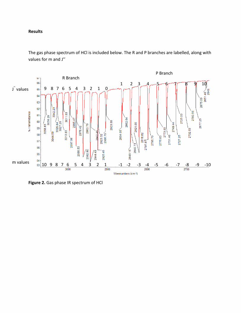
The gas phase spectrum of HCl is included below. The R and P branches are labelled, along with

values for m and J’’

Figure 2. Gas phase IR spectrum of HCl

R Branch

9 8 7 6 5 4 3 2 1 0 J’’ values

P Branch

1 2 3 4 5 6 7 8 9 10

m values 10 9 8 7 6 5 4 3 2 1

-1 -2 -3 -4 -5 -6 -7 -8 -9 -10

H35Cl data

The spectral data for H35Cl is tabulated below and then plotted as 𝜈 vs. m.

m 𝜈, 𝑐𝑚−1 10 3058.83

9 3044.58

8 3029.64

7 3013.93

6 2997.56

5 2980.53

4 2962.80

3 2944.43

2 2925.45

1 2905.79

-1 2864.65

-2 2843.15

-3 2821.09

-4 2797.87

-5 2775.00

-6 2751.40

-7 2727.25

-8 2702.53

-9 2677.25

-10 2651.40

Table 1. Tabulated spectral data for H35Cl

The graph of 𝜈 vs. m is fitted to a second order polynomial. The values of 𝜈0, 𝐵𝑒 , and 𝛼𝑒 are

determined from the polynomial fit using equation 1:

��(𝑚) = 𝜈0 + (2𝐵𝑒 − 2𝛼𝑒)𝑚 − 𝛼𝑒𝑚2

The values of 𝐼𝑒 and 𝑟𝑒 are also calculated. All values are tabulated and compared to literature

data.

Figure 3. Second order polynomial fit for spectral data of H35Cl

Value Experimental Literature7 Percent error

𝜈0, 𝑐𝑚−1 2,885.4205 2885.9775 0.0193 %

𝐵𝑒 , 𝑐𝑚−1 10.5264 10.593404 0.633 %

𝛼𝑒 , 𝑐𝑚−1 0.3030 -0.307139 1.35 %

𝐼𝑒 , 𝑘𝑔 𝑚2 2.65742 ∙ 10−47 2.64061 ∙ 10−47 0.637 %

𝑟𝑒 , 𝑝𝑚 127.815 127.455 0.283 %

Table 2. Values obtained from figure 3 compared to literature data

𝐼𝑒 and 𝑟𝑒 are calculated using equations 3 and 4 below.

𝐼𝑒 =ℎ

8𝜋2𝐵𝑒𝑐=

6.626 ∙ 10−34𝐽 𝑠

8𝜋2 ∙ 10.534 𝑐𝑚−1 ∙ 3 ∙ 1010 𝑐𝑚𝑠

= 2.65742 ∙ 10−47𝑘𝑔 𝑚2

𝜇 =𝑚1𝑚2

𝑚1 + 𝑚2=

1.007825 ∙ 34.968853

1.007825 + 34.968853= 0.979593

0.979593 ∙ 1.66054 ∙ 10−27𝑘𝑔 = 1.62665 ∙ 10−27𝑘𝑔

𝑟𝑒 = √𝐼

𝜇= √

2.65742 ∙ 10−47𝑘𝑔 𝑚2

1.62665 ∙ 10−27𝑘𝑔= 127.815 𝑝𝑚

y = -0.3030x2 + 20.4468x + 2,885.4205 R² = 1.0000

2600

2650

2700

2750

2800

2850

2900

2950

3000

3050

3100

-15 -10 -5 0 5 10 15

Wav

en

um

be

r, c

m-1

m

H35Cl, ṽ vs. m

H35Cl

Poly. (H35Cl)

The above calculations are repeated using a 3rd order polynomial fit in order to include the

centrifugal distortion constant, 𝐷𝑒, as seen in equation 2 below.

��(𝑚) = 𝜈0 + (2𝐵𝑒 − 2𝛼𝑒)𝑚 − 𝛼𝑒𝑚2 − 4𝐷𝑒𝑚3

Figure 4. Third order polynomial fit for spectral data of H35Cl


𝜈0, 𝑐𝑚−1 2,885.4205 2885.9775 0.0193 %

𝐵𝑒 , 𝑐𝑚−1 10.6047 10.593404 0.107 %

𝛼𝑒 , 𝑐𝑚−1 0.3030 -0.307139 1.35 %

𝐷𝑒 5.951 ∙ 10−4 −5.32019 ∙ 10−4 11.9 %

𝐼𝑒 , 𝑘𝑔 𝑚2 2.6378 ∙ 10−47 2.64061 ∙ 10−47 0.106 %

𝑟𝑒 , 𝑝𝑚 127.004 127.455 0.354 %



𝐼𝑒 =ℎ

8𝜋2𝐵𝑒𝑐=

6.626 ∙ 10−34𝐽 𝑠

8𝜋2 ∙ 10.6649 𝑐𝑚−1 ∙ 3 ∙ 1010 𝑐𝑚𝑠

= 2.62378 ∙ 10−47𝑘𝑔 𝑚2

𝑟𝑒 = √𝐼

𝜇= √

2.62378 ∙ 10−47𝑘𝑔 𝑚2

1.62665 ∙ 10−27𝑘𝑔= 127.004 𝑝𝑚

y = -0.0023804x3 - 0.3030x2 + 20.6034x + 2,885.4205 R² = 1.0000

2600

2650

2700

2750

2800

2850

2900

2950

3000

3050

3100

-15 -10 -5 0 5 10 15

Wav

en

um

be

r, c

m-1

m

H35Cl, ṽ vs. m

H35Cl

Poly. (H35Cl)

H37Cl data

The spectral data for H37Cl is tabulated below and then plotted as 𝜈 vs. m.

m 𝜈, 𝑐𝑚−1 10 3056.29

9 3042.23

8 3027.28

7 3011.63

6 2995.47

5 2978.42

4 2960.78

3 2942.46

2 2923.32

1 2903.80

-1 2862.64

-2 2840.73

-3 2818.82

-4 2795.87

-5 2773.03

-6 2749.44

-7 2725.00

-8 2700.56

-9 2675.00

-10 2649.00

Table 4. Tabulated spectral data for H37Cl

The graph of 𝜈 vs. m is fitted to a second order polynomial. The values of 𝜈0, 𝐵𝑒 , and 𝛼𝑒 are

determined from the polynomial fit using equation 1:

��(𝑚) = 𝜈0 + (2𝐵𝑒 − 2𝛼𝑒)𝑚 − 𝛼𝑒𝑚2

The values of 𝐼𝑒 and 𝑟𝑒 are also calculated. All values are tabulated and compared to literature

data.

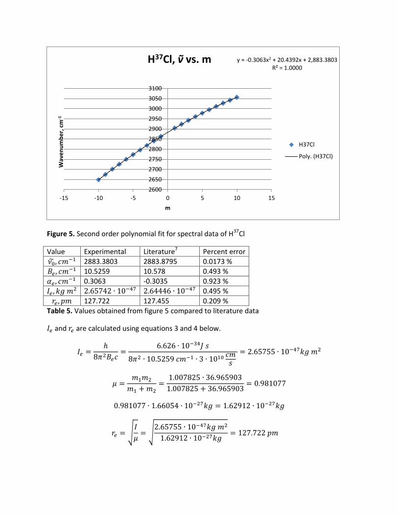
Figure 5. Second order polynomial fit for spectral data of H37Cl


𝜈0, 𝑐𝑚−1 2883.3803 2883.8795 0.0173 %

𝐵𝑒 , 𝑐𝑚−1 10.5259 10.578 0.493 %

𝛼𝑒 , 𝑐𝑚−1 0.3063 -0.3035 0.923 %

𝐼𝑒 , 𝑘𝑔 𝑚2 2.65742 ∙ 10−47 2.64446 ∙ 10−47 0.495 %

𝑟𝑒 , 𝑝𝑚 127.722 127.455 0.209 %



𝐼𝑒 =ℎ

8𝜋2𝐵𝑒𝑐=

6.626 ∙ 10−34𝐽 𝑠

8𝜋2 ∙ 10.5259 𝑐𝑚−1 ∙ 3 ∙ 1010 𝑐𝑚𝑠

= 2.65755 ∙ 10−47𝑘𝑔 𝑚2

𝜇 =𝑚1𝑚2

𝑚1 + 𝑚2=

1.007825 ∙ 36.965903

1.007825 + 36.965903= 0.981077

0.981077 ∙ 1.66054 ∙ 10−27𝑘𝑔 = 1.62912 ∙ 10−27𝑘𝑔

𝑟𝑒 = √𝐼

𝜇= √

2.65755 ∙ 10−47𝑘𝑔 𝑚2

1.62912 ∙ 10−27𝑘𝑔= 127.722 𝑝𝑚

y = -0.3063x2 + 20.4392x + 2,883.3803 R² = 1.0000

2600

2650

2700

2750

2800

2850

2900

2950

3000

3050

3100

-15 -10 -5 0 5 10 15

Wav

en

um

be

r, c

m-1

m

H37Cl, ṽ vs. m

H37Cl

Poly. (H37Cl)

The above calculations are repeated using a 3rd order polynomial fit in order to include the

centrifugal distortion constant, 𝐷𝑒, as seen in equation 2 below.

��(𝑚) = 𝜈0 + (2𝐵𝑒 − 2𝛼𝑒)𝑚 − 𝛼𝑒𝑚2 − 4𝐷𝑒𝑚3

Figure 6. Third order polynomial fit for spectral data of H37Cl


𝜈0, 𝑐𝑚−1 2883.3803 2883.8795 0.0173 %

𝐵𝑒 , 𝑐𝑚−1 10.6086 10.578 0.289 %

𝛼𝑒 , 𝑐𝑚−1 0.3063 -0.3035 0.923 %

𝐷𝑒 6.28 ∙ 10−4 5.30 ∙ 10−4 18.5 %

𝐼𝑒 , 𝑘𝑔 𝑚2 2.63686 ∙ 10−47 2.64446 ∙ 10−47 0.287 %

𝑟𝑒 , 𝑝𝑚 127.223 127.455 0.182 %



𝐼𝑒 =ℎ

8𝜋2𝐵𝑒𝑐=

6.626 ∙ 10−34𝐽 𝑠

8𝜋2 ∙ 10.6086 𝑐𝑚−1 ∙ 3 ∙ 1010 𝑐𝑚𝑠

= 2.63686 ∙ 10−47𝑘𝑔 𝑚2

𝑟𝑒 = √𝐼

𝜇= √

2.63686 ∙ 10−47𝑘𝑔 𝑚2

1.62912 ∙ 10−27𝑘𝑔= 127.32 𝑝𝑚

y = -0.0025129x3 - 0.3063x2 + 20.6045x + 2,883.3803 R² = 1.0000

2600

2650

2700

2750

2800

2850

2900

2950

3000

3050

3100

-15 -10 -5 0 5 10 15

Wav

en

um

be

r, c

m-1

m

H37Cl, ṽ vs. m

H37Cl

Poly. (H37Cl)

The value of 𝜈0 was determined above to be 2,885.4205 cm-1 for H35Cl and 2883.3803 cm-1 for

H37Cl. The values for 𝜈�� and 𝜈��𝜒𝑒 can be determined by simultaneously solving equations 5 and

6 below:

𝜈0 = 𝜈�� − 2𝜈��𝜒𝑒

2.885.4205 𝑐𝑚−1 = 𝜈�� − 2𝜈��𝜒𝑒

𝜈��𝜒𝑒 =𝜈��

2− 1442.71 𝑐𝑚−1

and

𝜈0∗ = 𝜈�� (

𝜇

𝜇∗)

12

− 2𝜈��𝜒𝑒

𝜇

𝜇∗

2,883.3803 𝑐𝑚−1 = 𝜈�� ∙ 0.999242 − 1.99697𝜈��𝜒𝑒

𝜈��𝜒𝑒 = 𝜈�� ∙ 0.50038 − 1443.88 𝑐𝑚−1

Combining these two equations gives:

𝜈��

2− 1442.71 𝑐𝑚−1 = 𝜈�� ∙ 0.50038 − 1443.88 𝑐𝑚−1

𝜈�� = 3081.76 𝑐𝑚−1

𝜈��𝜒𝑒 = 𝜈�� ∙ 0.50038 − 1443.88 𝑐𝑚−1 = 98.17 𝑐𝑚−1

Value Experimental Literature7 % error

𝜈�� 3081.76 2990.97424 3.04 %

𝜈��𝜒𝑒 98.17 52.84579 85.8 %

Table 7. Experimental values of 𝜈��𝜒𝑒 and 𝜈�� compared to literature values.

Potential sources of error could be differences in instrumentation used in literature values or

calibration errors.

Discussion

There is no absorption feature at the

𝜈0 value because this represents a

forbidden transition. This transition is from

𝐽′′ = 0 to 𝐽′′ = 0 which violates the

selection rule of allowed transitions being

Δ𝐽 = ±1.

An anharmonic oscillator does not

fit well to our data because the value of

anharmonicity constant 𝜈��𝜒𝑒 is not close to

the literature value. We can determine

from this that the molecule does not

demonstrate much anharmonicity.

The inclusion of centrifugal

distortion does not significantly improve

our results. Comparing tables 2 and 3, the

values of 𝐵𝑒 and 𝐼𝑒 are improved slightly by

including centrifugal distortion, but the

value for 𝑟𝑒 is slightly better without

including it. A slight improvement is seen in

all three values when comparing table 5 and

6. None of these differences however are

significant, therefore we can determine that

centrifugal stretching does not play an

important role.

Our data give the value for 𝐵𝑒

∗

𝐵𝑒=

0.999632. According to the rigid rotor

prediction, equation 7 is true, 𝐵𝑒

∗

𝐵𝑒=

𝜇

𝜇∗ =

0.999242. Our experimental value is very

accurate with only 0.0390 % error, which

suggests that our data corresponds very

well to a rigid rotor. The very small error

suggests that our data is very precise.

Acknowledgements

Thanks are given to Bob Jones

University Dr. George Matzko for his

supervision of laboratory procedures, and

to my 4 lab partners Eric Boley, Liz Chu,

Erica Cosmos, and David Maloney for their

assistance in experimental procedures.

Author Information Corresponding Author

[email protected]

Bob Jones University, Box 40343

References

1. Calvo, F.; Basire, M.; Parneix, P.

Temperature Effects on the Rovibrational

Spectra of Pyrene-Based PAHs. J. Phys.

Chem. A, 2011, 115, 8845–8854.

2. Fajardo, M. E. High-Resolution

Rovibrational Spectroscopy of Carbon

Monoxide Isotopologues Isolated in Solid

Parahydrogen. J. Phys. Chem. A, 2013, 117,

13504−13512.

3. Buckingham, G. T.; Chang, C.; Nesbitt, D.

J. High-Resolution Rovibrational

Spectroscopy of Jet-Cooled Phenyl Radical:

The ν19 Out-of-Phase Symmetric CH

Stretch. J. Phys. Chem. A, 2013, 117,

10047−10057.

4. Robertson, E. G.; Medcraft, C.;

McNaughton, D.; Appadoo, D. The Limits of

Rovibrational Analysis: The Severely

Entangled ν1 Polyad Vibration of

Dichlorodifluoromethane in the

Greenhouse IR Window. J. Phys. Chem. A

2014, 118, 10944−10954.

5. Muller, H. S. P.; Spezzano, S.; Bizzocchi ,

L.; Gottlieb, C. A.; Esposti, C. D.; McCarthy,

M. C. Rotational Spectroscopy of

Isotopologues of Silicon Monoxide, SiO, and

Spectroscopic Parameters from a Combined

Fit of Rotational and Rovibrational Data. J.

Phys. Chem. A 2013, 117, 13843−13854.

6. Garland, Carl W.; Nibler, Joseph W.;

Shoemaker, David P.; Experiments in

Physical Chemistry. McGraw-Hill: New York,

2009; p. 416-23.

7. Sime, R. J.; Physical Chemistry: Methods,

Techniques, and Experiments. Philadelphia,

PA: Saunders College Publishing, 1990, 680.

Documents

Rovib