Embed Size (px)
Citation preview

Brigham Young UniversityBYU ScholarsArchive
All Theses and Dissertations
2018-03-01
Rotational Stiffness Models for Shallow EmbeddedColumn-to-Footing ConnectionsAshley Lauren SadlerBrigham Young University
Follow this and additional works at: https://scholarsarchive.byu.edu/etd
Part of the Civil and Environmental Engineering Commons
This Thesis is brought to you for free and open access by BYU ScholarsArchive. It has been accepted for inclusion in All Theses and Dissertations by anauthorized administrator of BYU ScholarsArchive. For more information, please contact [email protected], [email protected].
BYU ScholarsArchive CitationSadler, Ashley Lauren, "Rotational Stiffness Models for Shallow Embedded Column-to-Footing Connections" (2018). All Theses andDissertations. 6752.https://scholarsarchive.byu.edu/etd/6752

Rotational Stiffness Models for Shallow Embedded
Column-to-Footing Connections
Ashley Lauren Sadler
A thesis submitted to the faculty of Brigham Young University
in partial fulfillment of the requirements for the degree of
Master of Science
Paul W. Richards, Chair Fernando S. Fonseca
Kyle M. Rollins
Department of Civil and Environmental Engineering
Brigham Young University
Copyright © 2018 Ashley Lauren Sadler
All Rights Reserved

ABSTRACT
Rotational Stiffness Models for Shallow Embedded Column-to-Footing Connections
Ashley Lauren Sadler
Department of Civil and Environmental Engineering, BYU Master of Science
Shallow embedded steel column connections are widely used in steel buildings; however, there is insufficient research about this connection type to understand the actual rotational stiffness that the connection provides. Shallow embedded steel columns are when a steel column is anchored to the foundation slab and then unreinforced concrete is poured around the base plate and the base of the column. This thesis seeks to further quantify the rotational stiffness available in this type of connection due to the added concrete and improve an existing model in order to represent the rotational stiffness.
Existing data from two series of experiments on shallow embedded columns were used to validate and improve an existing rotational stiffness model. These two data sets were reduced in the same manner so that they could be compared to one another. In addition, the rotational stiffness for each test column was determined so they could be evaluated against the outputs of the model. The existing model was improved by evaluating each parameter in the model: the modulus of subgrade reaction, exposed column length, modulus of concrete for the blockout and the foundation slab, flange effective width, embedment depth, and effective column depth. It was determined that the model was sensitive to the subgrade reaction, modulus of concrete, embedment depth and effective column depth. The exposed length was not a highly sensitive parameter to the model. Flange effective width was determined to not be needed, especially when the other parameters were altered. In order to test the sensitivity of the total stiffness to the rotational stiffness, equations were developed using the stiffness method for several different moment frame configurations with partial fixity at the column base. It was seen that if the rotational stiffness was changed by 100% then there could be seen a change in the total stiffness was only up to 20%.
Keywords: steel columns, shallowly embedded connections, rotational stiffness, blockout

ACKNOWLEDGEMENTS
This thesis would not have been possible without the support of several people, which I
would like to thank. I would like to first acknowledge the constant support and advice from my
committee chair Dr. Paul Richards. Without his time and effort this research would not have
progressed as much as it did. I would also like to thank my family and friends for their constant
support and encouragement. Finally, I want to thank the American Institute of Steel
Construction which provided funding for this project.
iv
TABLE OF CONTENTS
LIST OF TABLES ......................................................................................................................... vi
LIST OF FIGURES ...................................................................................................................... vii
1 Introduction ............................................................................................................................. 1
Overview of Steel Column-to-Footing Connections ........................................................ 1
Motivation ........................................................................................................................ 2
Scope of Research ............................................................................................................ 3
Outline .............................................................................................................................. 3
2 Literature Review .................................................................................................................... 4
Exposed Column Base Plate Connections ....................................................................... 4
2.1.1 DeWolf and Sarisley (1980) ....................................................................................... 4
2.1.2 Kanvinde and Deierlein (2011) ................................................................................... 6
2.1.3 Kanvinde et al. (2011)................................................................................................. 8
2.1.4 Kanvinde et al. (2013)................................................................................................. 9
Embedded Column Connections .................................................................................... 10
2.2.1 Cui et al. (2009) ........................................................................................................ 10
2.2.2 Grilli and Kanvinde (2015) ....................................................................................... 12
2.2.3 Barnwell (2015) ........................................................................................................ 13
2.2.4 Tryon (2016) ............................................................................................................. 15
2.2.5 Hanks (2016) ............................................................................................................. 19
2.2.6 Grilli and Kanvinde (2017) ....................................................................................... 22
2.2.7 Rodas, et al. (2017) ................................................................................................... 25
3 Data Reduction ...................................................................................................................... 27
Introduction .................................................................................................................... 27
Generating Hysteretic Plots ............................................................................................ 27
Calculating Effective Rotational Stiffness ..................................................................... 32
Results ............................................................................................................................ 34
Summary ........................................................................................................................ 43
4 Modified Tryon Model .......................................................................................................... 45
Introduction .................................................................................................................... 45
Influence of Various Parameters in Tryon’s Model ....................................................... 46
4.2.1 Effects of Exposed Lengths ...................................................................................... 46
v
4.2.2 Effects of Flange Effective Width ............................................................................ 48
4.2.3 Effects of Concrete Modulus .................................................................................... 50
Combined Effects ........................................................................................................... 52
4.3.1 Barnwell’s Data ........................................................................................................ 52
4.3.2 Hanks’ Data .............................................................................................................. 53
4.3.3 Direct Comparison .................................................................................................... 57
Summary ........................................................................................................................ 58
5 System Level Sensitivity ....................................................................................................... 60
Introduction .................................................................................................................... 60
Method ........................................................................................................................... 60
5.2.1 Sensitivity of Total Stiffness as Modulus of Subgrade Reaction Changes ............... 60
5.2.2 Sensitivity of Total Stiffness as the Rotational Stiffness β Changes ........................ 61
5.2.3 Sensitivity Analysis for Larger Moment Frame Systems ......................................... 64
Results ............................................................................................................................ 67
5.3.1 Sensitivity of Total Stiffness as Modulus of Subgrade Reaction Changes ............... 67
5.3.2 Sensitivity of Total Stiffness as the Rotational Stiffness β Changes ........................ 68
5.3.3 Sensitivity Analysis for Larger Moment Frame Systems ......................................... 74
Summary ........................................................................................................................ 84
6 Conclusions ........................................................................................................................... 85
References ..................................................................................................................................... 87
Appendix A ................................................................................................................................... 89

vi
LIST OF TABLES
Table 2-1: Specimen Test Matrix and Results (DeWolf and Sarisley 1980) .................................. 5
Table 2-2: Specimen Test Matrix (Grilli and Kanvinde 2015) ..................................................... 12
Table 2-3: Original Specimen Test Matrix (Barnwell 2015) ........................................................ 14
Table 2-4: Retested Specimen Test Matrix (Barnwell 2015) ....................................................... 15
Table 2-5: Specimen Test Matrix (Hanks 2016)........................................................................... 21
Table 3-1: Barnwell's Experiment Parameters .............................................................................. 29
Table 3-2: Hanks' Experimental Parameters ................................................................................. 29
Table 3-3: Rotational Stiffness Values from Barnwell's Experiments ......................................... 43
Table 3-4: Rotational Stiffness Values from Hanks’ Experiments ............................................... 43
Table 5-1: W8x35 Percent Change Comparison of Stiffness ....................................................... 71
Table 5-2: W10x77 Percent Change Comparison of Stiffness ..................................................... 74
Table 5-3: W8x35 Exterior Percent Change Comparison of Stiffness ......................................... 76
Table 5-4: W8x35 Interior Percent Change Comparison of Stiffness .......................................... 79
Table 5-5: W10x77 Exterior Percent Change Comparison of Stiffness ...................................... 81
Table 5-6: W10x77 Interior Percent Change Comparison of Stiffness ........................................ 83
vii
LIST OF FIGURES
Figure 1-1: Blockout connection commonly used at the base of steel buildings. ........................... 1
Figure 1-2: Exposed base plate connection commonly used at the base of steel buildings. ........... 2
Figure 2-1: Base Plate Strength Methods (DeWolf and Sarisley 1980). ........................................ 5
Figure 2-2: Model of various deformation (Kanvinde et al. 2011). ................................................ 9
Figure 2-3: Barnwell's test setup used for first and second testing (Barnwell 2015). .................. 14
Figure 2-4: Model for embedded column connection (Tryon, 2016). .......................................... 16
Figure 2-5: Tryon’s model for effective flange width. (Tryon, 2016). ......................................... 17
Figure 2-6: Tryon’s model for rotational stiffness vs. normalized embedment depth for W10s
(Tryon 2016). ........................................................................................................... 18
Figure 2-7: Hanks' test set up (Hanks 2016). ................................................................................ 20
Figure 2-8: Idealization of moment transfer- (a) overall equilibrium and (b) explode detail. ...... 23
Figure 3-1: Hysteretic plot for Barnwell's specimens. .................................................................. 30
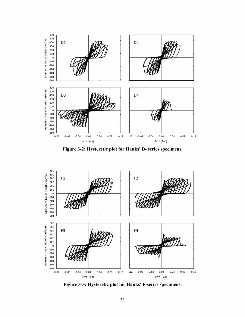
Figure 3-2: Hysteretic plot for Hanks' D- series specimens. ........................................................ 31
Figure 3-3: Hysteretic plot for Hanks' F-series specimens. .......................................................... 31
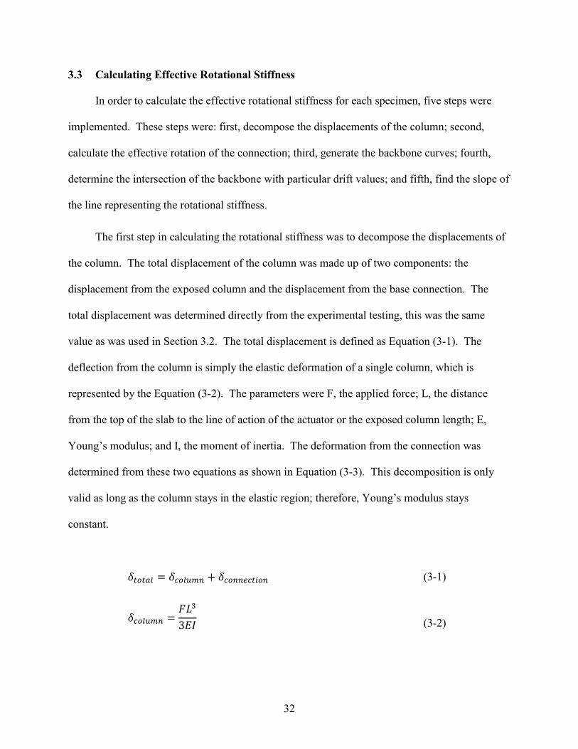
Figure 3-4: Specimen A2 rotational stiffness calculation. ............................................................ 34
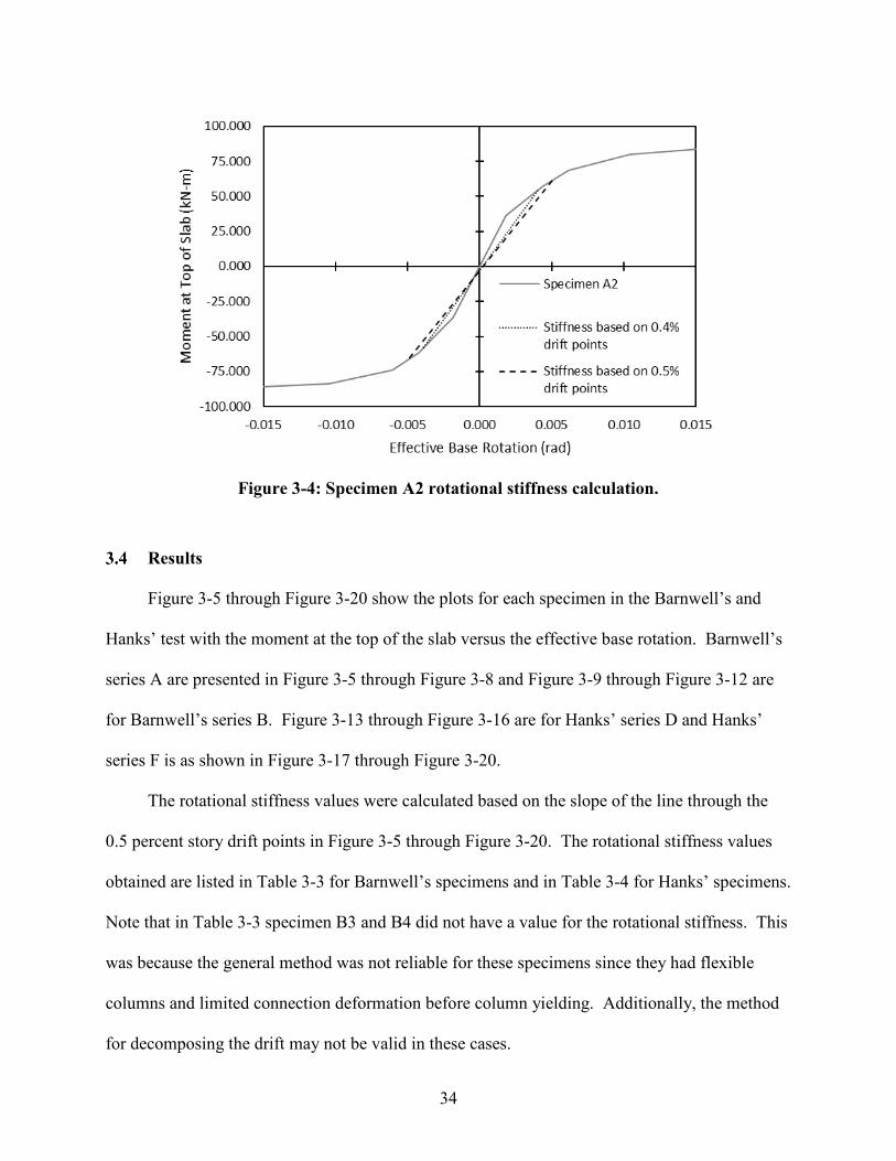
Figure 3-5: Specimen A1 moment at top of slab versus effective base rotation. (W8x35
Strong – 6.5 inches embedment depth). ................................................................... 35
Figure 3-6: Specimen A2 moment at top of slab versus effective base rotation (W8x48
Strong – 6.5 inches embedment depth). ................................................................... 35
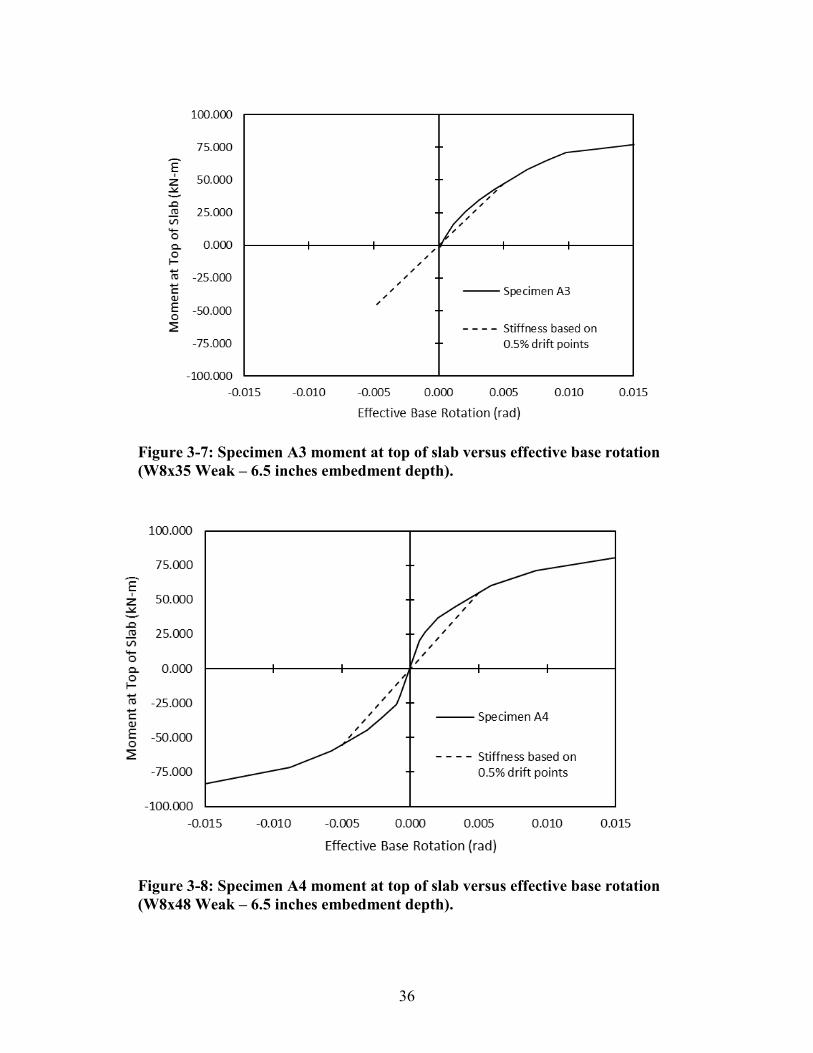
Figure 3-7: Specimen A3 moment at top of slab versus effective base rotation (W8x35
Weak – 6.5 inches embedment depth). .................................................................... 36
viii
Figure 3-8: Specimen A4 moment at top of slab versus effective base rotation (W8x48
Weak – 6.5 inches embedment depth). .................................................................... 36
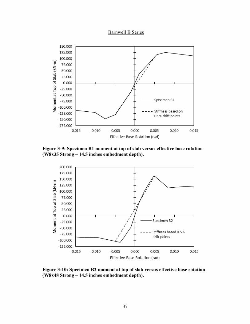
Figure 3-9: Specimen B1 moment at top of slab versus effective base rotation (W8x35
Strong – 14.5 inches embedment depth). ................................................................. 37
Figure 3-10: Specimen B2 moment at top of slab versus effective base rotation (W8x48
Strong – 14.5 inches embedment depth). ................................................................. 37
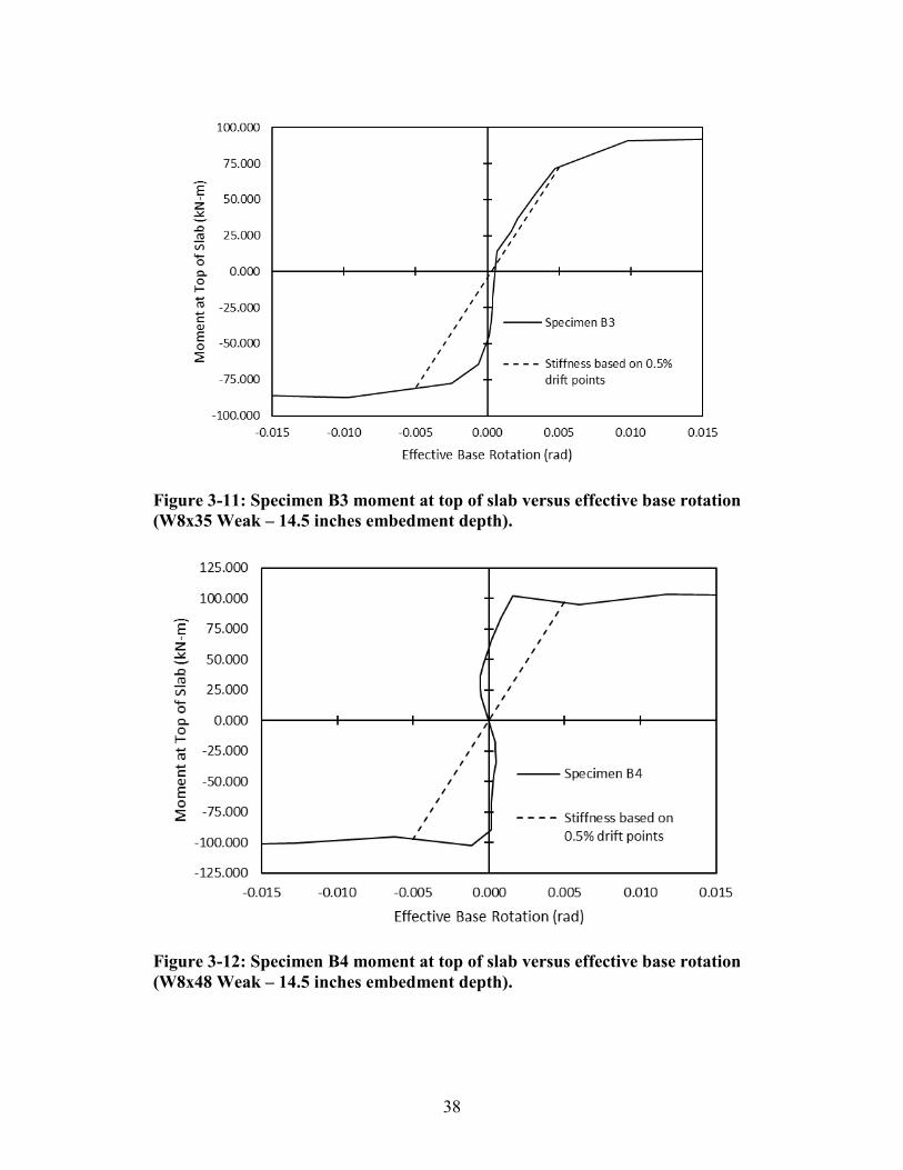
Figure 3-11: Specimen B3 moment at top of slab versus effective base rotation (W8x35
Weak – 14.5 inches embedment depth). .................................................................. 38
Figure 3-12: Specimen B4 moment at top of slab versus effective base rotation (W8x48
Weak – 14.5 inches embedment depth). .................................................................. 38
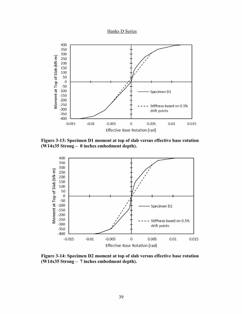
Figure 3-13: Specimen D1 moment at top of slab versus effective base rotation (W14x35
Strong – 0 inches embedment depth). ..................................................................... 39
Figure 3-14: Specimen D2 moment at top of slab versus effective base rotation (W14x35
Strong – 7 inches embedment depth). ..................................................................... 39
Figure 3-15: Specimen D3 moment at top of slab versus effective base rotation (W14x35
Strong – 15 inches embedment depth). .................................................................... 40
Figure 3-16: Specimen D4 moment at top of slab versus effective base rotation (W14x35
Strong – 15 inches embedment depth). .................................................................... 40
Figure 3-17: Specimen F1 moment at top of slab versus effective base rotation (W10x77
Strong – 0 inches embedment depth). ..................................................................... 41
Figure 3-18: Specimen F2 moment at top of slab versus effective base rotation (W10x77
Strong – 7 inches embedment depth). ..................................................................... 41
ix
Figure 3-19: Specimen F3 moment at top of slab versus effective base rotation (W10x77
Strong – 15 inches embedment depth). .................................................................... 42
Figure 3-20: Specimen F4 moment at top of slab versus effective base rotation (W10x77
Strong – 15 inches embedment depth). .................................................................... 42
Figure 4-1: Exposed length comparison for Barnwell’s experiments (ko = 150kip/in3). ............. 47
Figure 4-2: Exposed length comparison for Hanks’ experiments (ko = 150kip/in3). ................... 47
Figure 4-3: Flange effective width comparison of Barnwell's strong axis specimens
(ko = 150kip/in3). ...................................................................................................... 49
Figure 4-4: Flange effective width comparison of Hanks' specimens (ko = 150kip/in3). ............. 49
Figure 4-5: Barnwell's experiments compared to differing equations of the base plate
rotational stiffness, ks (ko = 150kip/in3). .................................................................. 51
Figure 4-6: Hanks' experiments compared to differing equations of the base plate rotational
stiffness, ks, (ko = 150kip/in3). .................................................................................. 51
Figure 4-7: Barnwell’s experiments compared to Tryon’s model using Equation 4-5. The
concrete footing modulus used was 3600 ksi and the concrete blockout modulus
used was 2280 ksi. ................................................................................................... 53
Figure 4-8: Hanks’ experiments compared to Tryon’s model using Equation 4-5. The
concrete footing blockout moduli were 3600 ksi. .................................................... 54
Figure 4-9: Hanks’ experiment compared to Tryon’s model using Equation 4-5 for multiple
values of ko. The concrete footing and blockout moduli were 3600 ksi. ................ 54
Figure 4-10: Hanks’ experiments compared to Tryon’s model using Equation 4-5 when d is
the distance between anchor bolts. The concrete footing and blockout moduli
were 3600 ksi. .......................................................................................................... 55
x
Figure 4-11: Hanks’ experiment compared to Tryon’s model using Equation 4-5 when d is
the distance between anchor bolts and with multiple ko. The concrete footing
and blockout moduli are 3600 ksi. ........................................................................... 56
Figure 4-12: Exposed length comparison for Hanks’ experiments when d is the distance
between anchor bolts. d = 16 inches for W10 and d = 18 inches for W14
(ko = 150 kip/in3). ..................................................................................................... 57
Figure 4-13: Comparison of Tryon's original model to the modified model with Barnwell's
specimens (ko=150 kip/in3). ..................................................................................... 58
Figure 4-14: Comparison of Tryon's original model to the modified model with Hanks'
specimens (ko=200 kip/in3). ..................................................................................... 58
Figure 5-1: Full moment frame and system parameters with partial fixity denoted at the top
of the slab. ................................................................................................................ 62
Figure 5-2: Half the moment frame and system parameters for the system analyzed with
partial fixity denoted at the top of the slab. ............................................................. 62
Figure 5-3: The four degrees of freedom and nodes for the half moment frame. ......................... 62
Figure 5-4: Multi-story and bay moment frame with system parameters labeled and partial
fixity denoted at each top of the slab. ...................................................................... 64
Figure 5-5: Exterior element of a multi-story and bay moment frame with system parameters
labeled and partial fixity noted at the top of the slab. .............................................. 65
Figure 5-6: Interior element of multi-story and bay moment frame with system parameters
labeled and partial fixity noted at the top of the slab. .............................................. 65
Figure 5-7: Six degrees of freedom for the exterior elements of a multi-story and bay moment
frame as used in analysis.......................................................................................... 66
xi
Figure 5-8: Seven degrees of freedom for the interior elements of a multi-story and bay
moment frame as used in analysis. .......................................................................... 66
Figure 5-9: Barnwell’s W8x35 14.5 inches embedment depth - single column stiffness
analysis. .................................................................................................................... 68
Figure 5-10: Comparison of stiffness for W8x35 of 6.5 inches embedment depth for a large
range of rotational stiffness. ..................................................................................... 69
Figure 5-11: Comparison of stiffness for W8x35 of 6.5 inches embedment depth from
Barnwell's experiments and Tryon's model for a partially fixed moment frame ..... 70
Figure 5-12: Comparison of stiffness for W8x35 of 14.5 inches embedment depth from
Barnwell's experiments and Tryon's model for a partially fixed moment frame. .... 71
Figure 5-13: Comparison of stiffness for W10x77 of 7 inches embedment depth from Hanks’
experiments and Tryon's model for a partially fixed moment frame. ...................... 72
Figure 5-14: Comparison of stiffness for W10x77 of 15 inches embedment depth from Hanks’
experiments and Tryon's model for a partially fixed moment frame. ...................... 73
Figure 5-15: Plot of total stiffness versus rotational stiffness for exterior assembly (W8x35 –
6.5 inches embedment depth). ................................................................................. 75
Figure 5-16: Plot of total stiffness versus rotational stiffness for exterior assembly (W8x35 –
14.5 inches embedment depth). ............................................................................... 76
Figure 5-17: Plot of total stiffness versus rotational stiffness for interior assembly (W8x35 –
6.5 inches embedment depth). ................................................................................. 77
Figure 5-18: Plot of total stiffness versus rotational stiffness for interior assembly (W8x35 –
14.5 inches embedment depth). ............................................................................... 78

xii
Figure 5-19: Plot of total stiffness versus rotational stiffness for exterior assembly (W10x77 –
7 inches embedment depth). .................................................................................... 80
Figure 5-20: Plot of total stiffness versus rotational stiffness for exterior assembly (W10x77 –
15 inches embedment depth). .................................................................................. 81
Figure 5-21: Plot of total stiffness versus rotational stiffness for interior assembly (W10x77 –
7 inches embedment depth). .................................................................................... 82
Figure 5-22: Plot of total stiffness versus rotational stiffness for interior assembly (W10x77 –
15 inches embedment depth). .................................................................................. 83

1
1 INTRODUCTION
Overview of Steel Column-to-Footing Connections
Steel is one of the most affordable and durable materials, which is why it is commonly
used for framing multi-story buildings. Concrete is also an efficient material and is typically
used for the foundations of steel buildings. One of the most common connections in construction
is the connection of a steel column to a concrete footing. Figure 1-1 shows how this connection
is often accomplished, by leaving a square hole (blockout) in the floor slab, so that the steel
column can be bolted directly to the footing under the slab. After the column is installed the
square hole (blockout) is filled in with concrete, hiding the bolts and base plate; no extra
reinforcing steel is added in the blockout section.
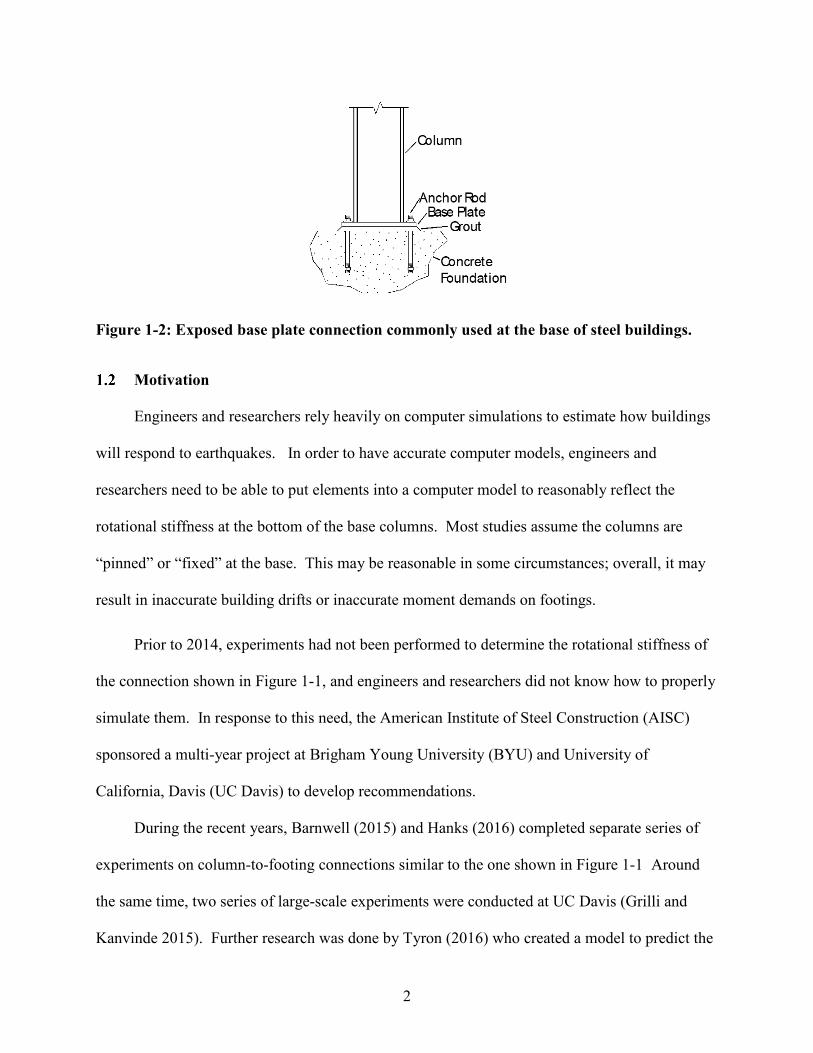
Figure 1-2 shows the configuration for another common steel column to concrete footing
connection, an exposed column base plate. It can be seen that the major difference between the
two figures is the blockout. The exposed base plate in Figure 1-2 does not have a concrete
blockout around the column and the base plate.
(a) (b)
Figure 1-1: Blockout connection commonly used at the base of steel buildings: (a) detail; (b) picture of blockout just after column installation and prior to pouring of blockout concrete.
Base PlateGrout
Anchor Rod
Column
ConcreteFoundation
Slab on Grade
Blockout
2
Figure 1-2: Exposed base plate connection commonly used at the base of steel buildings.
Motivation
Engineers and researchers rely heavily on computer simulations to estimate how buildings
will respond to earthquakes. In order to have accurate computer models, engineers and
researchers need to be able to put elements into a computer model to reasonably reflect the
rotational stiffness at the bottom of the base columns. Most studies assume the columns are
“pinned” or “fixed” at the base. This may be reasonable in some circumstances; overall, it may
result in inaccurate building drifts or inaccurate moment demands on footings.
Prior to 2014, experiments had not been performed to determine the rotational stiffness of
the connection shown in Figure 1-1, and engineers and researchers did not know how to properly
simulate them. In response to this need, the American Institute of Steel Construction (AISC)
sponsored a multi-year project at Brigham Young University (BYU) and University of
California, Davis (UC Davis) to develop recommendations.
During the recent years, Barnwell (2015) and Hanks (2016) completed separate series of
experiments on column-to-footing connections similar to the one shown in Figure 1-1 Around
the same time, two series of large-scale experiments were conducted at UC Davis (Grilli and
Kanvinde 2015). Further research was done by Tyron (2016) who created a model to predict the
3
rotational stiffness of such connections; he used values from Barnwell’s tests to calibrate his
model.
Scope of Research
The purpose of this research was to evaluate the recently generated experimental data
collectively, and to develop a rotational stiffness model that engineers and researchers can use in
computer models to simulate the response of buildings from earthquakes. Tryon’s original
model was refined based on observations from the experimental data.
The research that was accomplished can be separated into three sections. First, all recent
experimental data was evaluated; second, the existing mathematical model was refined to better
represent all of the data; and third, several moment frame configurations were evaluated with a
closed form solution of the total stiffness to determine the sensitivity of the rotational stiffness.
Outline
This chapter has included a brief introduction to the research that was conducted and to
introduce the motivation for additional research. Chapter 2 reviews the current literature on
column-to-footing connections. Chapter 3 describes the method used for data reduction of
Barnwell’s and Hanks’ data sets. The description of the modification of Tryon’s model is
discussed in Chapter 4. The system level sensitivity of different configurations and Tryon’s
modified model is discussed in Chapter 5. Finally, conclusions are presented in Chapter 6.

4
2 LITERATURE REVIEW
Exposed Column Base Plate Connections
Exposed base plate connections were introduced in Section 1.1 (Figure 1-1). A great deal
of research has been performed on these connections and the models are fairly accurate in
predicting the rotational stiffness. Even though these models are not perfect for embedded
columns, they provide a good starting point for the interaction of the base plate and concrete
foundation.
2.1.1 DeWolf and Sarisley (1980)
DeWolf and Sarisley (1980), investigated the strength of exposed base plate connections.
They used two methods, the working stress and the ultimate strength methods, to determine the
strength of the connections. Figure 2-1 shows the compression block for both methods. They
conducted 16 tests to compare the models’ results, Table 2-1 shows the test matrix. The 16
specimens were tested by inducing a moment on the column from an axial load with an
eccentricity. The main differences between the two models were the compression block. The
working stress method had a triangular distributed bearing stress and the ultimate strength
method was modeled as a rectangular stress block. The average factor of safety was 2.16 for the
working stress method and 1.11 for the ultimate strength method.

5
Table 2-1: Specimen Test Matrix and Results (DeWolf and Sarisley 1980)
(a) Working stress Method b) Ultimate Strength Method
Figure 2-1: Base Plate Strength Methods (DeWolf and Sarisley 1980).

6
The authors reached three conclusions from their experiments:
1. When the diameter of the anchor bolts was large in comparison to the base plate
dimensions, then the distance from the anchor bolt to the bearing zone of the plate
on the concrete was small. The smaller bearing area, did not allow the anchor bolt
to reach capacity, and therefore, some of the bolts were ineffective.
2. When the concrete area was greater than the base plate area, then a confining effect
needed to be accounted for in the design.
3. Increased plate thickness decreased capacity at a point, due to the plate acting like a
rigid plate and would cause premature failure. This was due to large bearing
stresses from the plate not being as flexible.
The authors recommended that the ultimate strength method be used for design, because it more
accurately predicted the connection behavior.
2.1.2 Kanvinde and Deierlein (2011)
Kanvinde and Deierlein (2011), conducted experiments on 20 exposed base plate
connections. These tests were meant to be compared to the AISC Design Guide (Fisher and
Kloiber 2006), which is the current standard for designing exposed column base plate
connections. They also were concerned with the behavior of the columns for three different
scenarios which were tested to failure: an applied axial load with an eccentricity to induce a
moment, an axial load and a shear force applied at the base of the column, and an axial and
moment loads on columns designed to isolate the column to base plate weld. The first two
mechanisms had seven specimens in the test series and the final mechanism had 6 specimens.
All specimens were constructed to two-third scale and then tested to failure.

7
The authors reached the following conclusions for each mechanism:
1. Moment Capacity
i. All tests showed “excellent deformation capacity” with little strength
degradation until after 7% - 10% drift. This suggested that the current
design assumption, i.e., the base plate remaining elastic, may be rather
conservative and significant deformation and energy dissipation capacity
were available in the base plate.
ii. The AISC Design Guide gave highly conservative predictions. It was
observed that the experimental data showed connection strengths that were
80% greater than the predicted values on average.
2. Shear Capacity
i. A coefficient of friction value of 0.45 was recommended to be used
between the grout and steel. This was slightly higher than the value
recommended in AISC Design Guide of 0.40.
ii. The AISC Design Guide was accurate for shear loads resisted by anchor
bolts. The bolts should be checked for the interaction between flexural
axial forces and direct axial loads.
iii. Concrete Capacity Design (CCD) was recommended for use in design
when a shear key or shear lug is used, since the current method of 45°
cone method was not conservative.

8
3. Weld Capacity
i. The Complete Joint Penetration (CJP) and Partial Joint Penetration (PJP)
were both adequate for use in seismic design, which could withstand up to
3% to 5% drift.
ii. PJP performed better than the CJP. This was attributed to the stress
concentrations that form around the access hole for the CJP groove weld.
2.1.3 Kanvinde et al. (2011)
Kanvinde et al. (2011) focused on the rotational stiffness of exposed column base
connections, due to the fact that this element is often ignored in the design process. They
developed an analytical model which was validated with nine experimental specimens.
Their method to estimate the design stiffness of base connections had three steps:
1. Determine the design strength and internal force distribution
2. Determine the deformation under high eccentricity
3. Calculate the connection rotation for each individual component
The components that contributed to the total deformation were the stretching of anchor rods that
were in tension, the bending of the plate on the tension and compression sides, and the
deformation of the concrete under the compression side of the plate; Figure 2-2 depicts these
different deformations.

9
Figure 2-2: Model of various deformation (Kanvinde et al. 2011).
The authors stated that the design of the connections cannot be classified as pinned or
fixed, for it was somewhere in the middle. The classification of the base fixity was important for
the design, for if the column was designed as fixed, then increased story drift could occur in the
first story. Additionally, if the connection was designed as pinned then it would be possible for a
more conservative response. Therefore, for safety and economy reasons it is important to
understand the true fixity of the connection.
The authors warned that there were a few inherent inaccuracies in the method that was
included from the AISC Design Guide (Fisher and Kloiber 2006). One of the main assumption
was the shape of the stress block. Both of these models assume that the stress block was
rectangular; however, this was not a perfect representation of the behavior.
2.1.4 Kanvinde et al. (2013)
Kanvinde et al. (2013) investigated the connection response of exposed base plate
connections by adjusting the base plate thickness. They noted that previous models had
simplified assumptions in order to perform tests, since it was extremely difficult to test
individual components due to the highly interactive nature of all the components. Therefore, the
10
authors performed finite element analysis in order to isolate single components. They then
validated the model with physical experiments.
From these comparisons, the authors noted that the current method for determining the
rotational stiffness may be adequate; however, a perfect prediction would be too complex for
normal design situations. It was additionally noted that the thickness of the base plate should be
a key factor in the design formulas since it was seen that a thicker base plate increased the
connection stiffness capacity.
The important finding from their finite element analysis was that the rectangular
compression block may be non-conservative for thicker plates since thicker plates tend to have
higher stress concentrations at the toe of the compression side of the base plate.
Embedded Column Connections
Embedded column connections were introduced in Section 1.1 (Figure 1-2) and are formed
by pouring concrete around the base of the column after the foundation and main slab have been
poured and the steel columns has been anchored into place. These connections are commonly
used due to the ease of construction as well as it being more aesthetically pleasing. However,
there is limited research on the behavior of this type of connection.
2.2.1 Cui et al. (2009)
Cui et al. (2009) conducted experiments to investigate the effect of earthquake loads on
shallow-embedded column base connections, specifically the effect on the slab. Their tests
included eight two-third scale HSS columns. They investigated the effects of slab thickness,
shape, and reinforcement on elastic stiffness, strength, and energy dissipation capacity of the
embedded column.

11
The test specimens were all constructed from HSS 200 mm tubes. Seven columns had 9
mm tube thickness and one column had 12 mm tube thickness. The base plates were all 25-mm
thick and 300 mm square. Each base plate had twelve anchor bolts spread evenly around the
base plate and the foundation was designed to be stiff enough that the anchor bolts governed the
strength. One of the specimens was left with an exposed base plate to act as the control. The
other seven had varying amounts of reinforcement and slab shapes. The columns were all loaded
axially with a 511 kN load.
The authors reasoned that the contribution of the concrete slab to resist the applied moment
was provided by two mechanisms: 1) The direct bearing of the slab on the column in
compression, and 2) Punching resistance of the slab from the rotation of the base plate.
The authors reached six conclusions from their experiments.
1. The elastic stiffness, maximum strength, and dissipated energy saw improvement
with the inclusion of the floor slab.
2. The thickness and shape of the floor slab caused significant changes in the
maximum strength. The inclusion of horizontal rebar also greatly improved the
strength.
3. Horizontal rebar increased the deformation capacity.
4. The main failure mode was punching shear in the column slab. This was true until
the column base connection strength was increased to be larger than the plastic
moment of the column, then the column failed in local buckling.
5. A strengthened slab and elevated foundation slab shape should be used.

12
6. The plastic theory could reasonably estimate the maximum strength of the column
regardless of thickness and geometric shape of the floor slab, with less than 20%
error.
2.2.2 Grilli and Kanvinde (2015)
Grilli and Kanvinde (2015) investigated the performance of embedded column base
connections under seismic loads. They tested five full scale test specimens with the
consideration of three main variables: embedment depth, column size, and axial load, Table 2-2
summarizes the tests conducted. The specimens were constructed by a welding a base plate to a
wide flange shape. They also welded a stiffener on the column where the blockout slab would
end. Their purpose was for the base plate to be used in uplift resistance and the stiffener for
compression resistance.
Table 2-2: Specimen Test Matrix (Grilli and Kanvinde 2015)
13
These experiments demonstrated that the strength and stiffness of the embedded column
were greater than that of the exposed base connection and that the stiffness increased as the
embedment depth increased. Another observation was that increased connection strength
occurred with increased flange width. In the experiments, there was a correlation between
compressive axial load and strength compared with that of no applied load; however, no
correlation was seen for a tensile load. Finally, strength and stiffness were seen to decrease as the
concrete cracked.
The authors also proposed a strength model calibrated from their experimental data. The
model was based on three mechanisms. The first was horizontal bearing stress that acts on the
column flanges. The second was the vertical bearing stresses that act on the embedded base plate
at the bottom of the column, and the third was panel shear. The authors suggested that their
model was applicable for deeper columns; however, for shallow embedment, a model like
Barnwell’s (2015) or any other model that was better suited. A final note by the authors was
about connection fixity. They stated that although their column connections were designed as if
they were fixed, there was still some flexibility in the connection, which should be accounted for
during design.
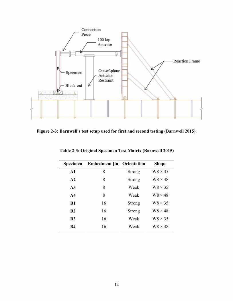
2.2.3 Barnwell (2015)
Figure 2-3 showed Barnwell’s test setup. He investigated shallow-embedded columns
with blockout concrete. The test matrix included twelve two-third scale specimens in order to
investigate the effect of the blockout concrete on the rotational stiffness and overall strength of
the connection. The original eight specimens are shown in Table 2-3. Four additional tests were
conducted on four of the eight original specimens as summarized in Table 2-4. All specimens
were tested to failure and had four anchor bolts located in the corners of the base plate.
14
Figure 2-3: Barnwell's test setup used for first and second testing (Barnwell 2015).
Table 2-3: Original Specimen Test Matrix (Barnwell 2015)
Specimen Embedment [in] Orientation Shape
A1 8 Strong W8 × 35
A2 8 Strong W8 × 48
A3 8 Weak W8 × 35
A4 8 Weak W8 × 48
B1 16 Strong W8 × 35
B2 16 Strong W8 × 48
B3 16 Weak W8 × 35
B4 16 Weak W8 × 48
15
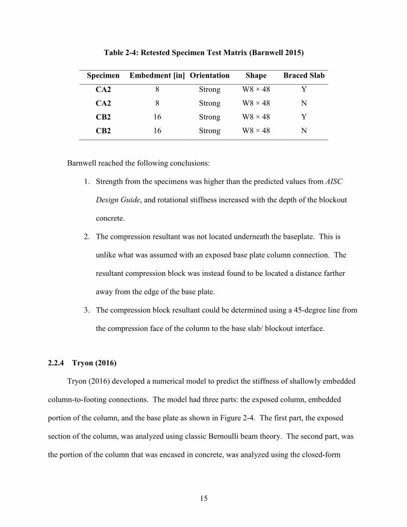
Table 2-4: Retested Specimen Test Matrix (Barnwell 2015)
Specimen Embedment [in] Orientation Shape Braced Slab
CA2 8 Strong W8 × 48 Y
CA2 8 Strong W8 × 48 N
CB2 16 Strong W8 × 48 Y
CB2 16 Strong W8 × 48 N
Barnwell reached the following conclusions:
1. Strength from the specimens was higher than the predicted values from AISC
Design Guide, and rotational stiffness increased with the depth of the blockout
concrete.
2. The compression resultant was not located underneath the baseplate. This is
unlike what was assumed with an exposed base plate column connection. The
resultant compression block was instead found to be located a distance farther
away from the edge of the base plate.
3. The compression block resultant could be determined using a 45-degree line from
the compression face of the column to the base slab/ blockout interface.
2.2.4 Tryon (2016)
Tryon (2016) developed a numerical model to predict the stiffness of shallowly embedded
column-to-footing connections. The model had three parts: the exposed column, embedded
portion of the column, and the base plate as shown in Figure 2-4. The first part, the exposed
section of the column, was analyzed using classic Bernoulli beam theory. The second part, was
the portion of the column that was encased in concrete, was analyzed using the closed-form
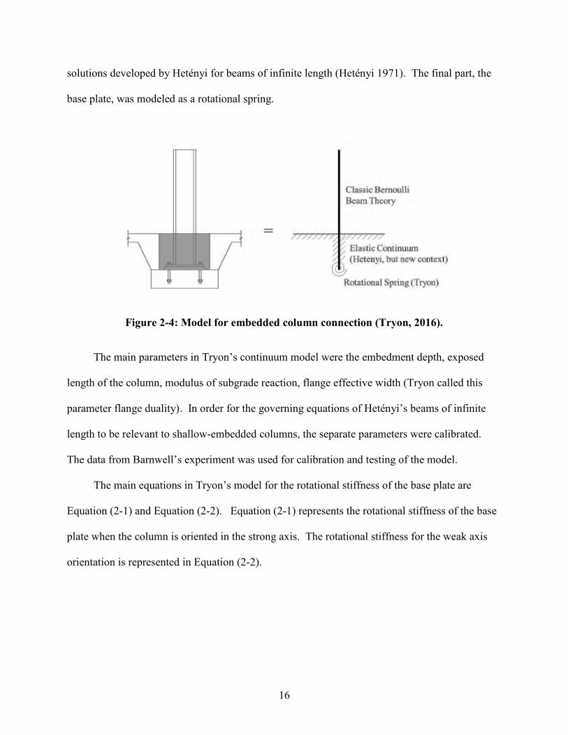
16
solutions developed by Hetényi for beams of infinite length (Hetényi 1971). The final part, the
base plate, was modeled as a rotational spring.
The main parameters in Tryon’s continuum model were the embedment depth, exposed
length of the column, modulus of subgrade reaction, flange effective width (Tryon called this
parameter flange duality). In order for the governing equations of Hetényi’s beams of infinite
length to be relevant to shallow-embedded columns, the separate parameters were calibrated.
The data from Barnwell’s experiment was used for calibration and testing of the model.
The main equations in Tryon’s model for the rotational stiffness of the base plate are
Equation (2-1) and Equation (2-2). Equation (2-1) represents the rotational stiffness of the base
plate when the column is oriented in the strong axis. The rotational stiffness for the weak axis
orientation is represented in Equation (2-2).
Figure 2-4: Model for embedded column connection (Tryon, 2016).

17
𝑘𝑘𝑠𝑠 =𝑘𝑘𝑑𝑑3
24�
𝑏𝑏𝑓𝑓2𝑏𝑏𝑓𝑓 − 𝑡𝑡𝑤𝑤
� �𝐸𝐸𝑓𝑓𝑓𝑓𝑓𝑓𝑓𝑓𝑓𝑓𝑓𝑓𝑓𝑓𝐸𝐸𝑏𝑏𝑏𝑏𝑓𝑓𝑏𝑏𝑏𝑏𝑓𝑓𝑏𝑏𝑓𝑓
+ 1� (2-1)
𝑘𝑘𝑠𝑠 =𝑘𝑘𝑏𝑏𝑓𝑓3
24�𝐸𝐸𝑓𝑓𝑓𝑓𝑓𝑓𝑓𝑓𝑓𝑓𝑓𝑓𝑓𝑓𝐸𝐸𝑏𝑏𝑏𝑏𝑓𝑓𝑏𝑏𝑏𝑏𝑓𝑓𝑏𝑏𝑓𝑓
+ 1� (2-2)
One parameter of interest was the flange effective width for the strong axis orientation.
This factor assumed that both flanges bearing against the concrete blockout acted in resisting.
Figure 2-5 shows the depiction of the dual flanges resisting against the concrete blockout. Tryon
accounted for the two flanges with the term �2𝑏𝑏𝑓𝑓 − 𝑡𝑡𝑤𝑤� in Equation (2-1). He incorporated the
flange effective width into the equations for base plates rotational stiffness. The flange effective
width is not included in Equation (2-2) because the weak axis orientation only has the depth of
the column resisting against the concrete blockout.
Tryon also accounted for the differing strength in the blockout concrete and the base slab
of concrete since these have an effect on the stiffness. This parameter is given in Equation (2-3),
which is the average of the two concrete strengths to the blockout modulus. However, the ratio
Figure 2-5: Tryon’s model for effective flange width. (Tryon, 2016).
12�𝐸𝐸𝑓𝑓𝑓𝑓𝑓𝑓𝑓𝑓𝑓𝑓𝑓𝑓𝑓𝑓𝐸𝐸𝑏𝑏𝑏𝑏𝑓𝑓𝑏𝑏𝑏𝑏𝑓𝑓𝑏𝑏𝑓𝑓
+ 1�
18
of the modulus of concretes would cancel out if the strength of the two were equal or close to
equal.
𝑘𝑘𝑠𝑠 =12�𝐸𝐸𝑓𝑓𝑓𝑓𝑓𝑓𝑓𝑓𝑓𝑓𝑓𝑓𝑓𝑓𝐸𝐸𝑏𝑏𝑏𝑏𝑓𝑓𝑏𝑏𝑏𝑏𝑓𝑓𝑏𝑏𝑓𝑓
+ 1� (2-3)
Tryon demonstrated that the rotational stiffness of the base plate was related to the
modulus of subgrade reaction. The stiffness of the concrete was determined by the modulus of
subgrade reaction multiplied with the depth of the column bearing against the concrete. This
meant that for a column loaded in the strong axis direction, the subgrade modulus was multiplied
by the flange width and the weak axis was multiplied by the depth of the column.
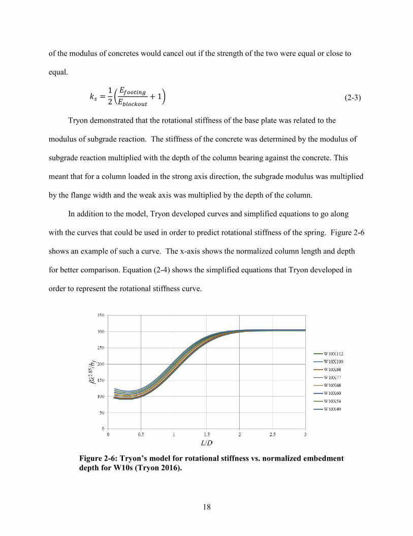
In addition to the model, Tryon developed curves and simplified equations to go along
with the curves that could be used in order to predict rotational stiffness of the spring. Figure 2-6
shows an example of such a curve. The x-axis shows the normalized column length and depth
for better comparison. Equation (2-4) shows the simplified equations that Tryon developed in
order to represent the rotational stiffness curve.
Figure 2-6: Tryon’s model for rotational stiffness vs. normalized embedment depth for W10s (Tryon 2016).

19
2.85
0.50135
110 80 0.5 2.0
300 2.0f
LD
L Lb D D
LD
βλ
<= ⋅ + ≤ < ≤
(2-4)
Where:
β = Rotational stiffness at the embedment concrete (kip-in/radians)
bf = Width of column flange (in)
L = Embedment depth of the column (in)
D = Depth of the column (in)
λ = Factor that incorporates the material properties of both the embedment material and the column material.
04
(2 )4
f w
x
k b tE I⋅ −
⋅ ⋅
ko = modulus of reaction of the embedment material, assumed to be = 500 kip/in3
tw = web thickness of column (in)
E = Modulus of Elasticity of column material = 29000 ksi
Ix = Moment of Inertia of the column about its strong axis (in4)
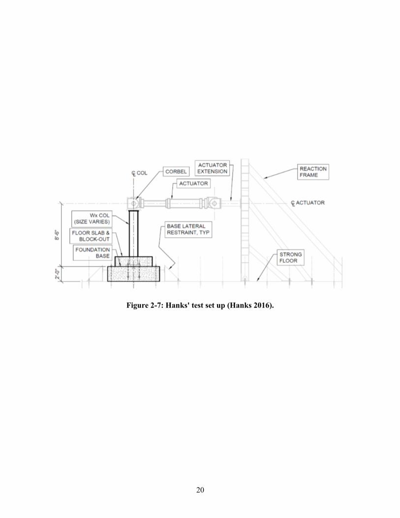
2.2.5 Hanks (2016)
Hanks (2016) validated the model proposed by Barnwell (2015) as well as studied the
effects of the stiffness of shallow embedded moment frame columns on the ductility of the
frame. He constructed eight two-third scale test specimens, which were similar in design to
Barnwell’s specimens. Hanks’ test set up was also quite similar to Barnwell’s as shown in
Figure 2-7.
20
Figure 2-7: Hanks' test set up (Hanks 2016).

21
The eight specimens were divided into two series of tests; each series being defined by a
different column size. The first specimen in each series acted as the control, i.e., specimens with
no blockout concrete and only an exposed base plate connection. The second specimen in each
series had a blockout with a depth of 8 inches. The third and fourth specimens had blockouts
that were 16 inches deep. The difference between the third and fourth specimens in the series
was the number of anchor bolts. The full test matrix is shown in Table 2-5. The number of
anchor bolts used in each connection was one of the key changes from Barnwell’s tests.
Additional differences between Hanks’ experiment and Barnwell’s was the inclusion of a shear
tab at the bottom of the base plate as well as larger column sizes.
Table 2-5: Specimen Test Matrix (Hanks 2016)
Column Base Plate Anchor Bolts Base Block-out
Specimen Name Size Thickness
(in) ASTM grade
Shear Lug Qty DIA
(in) Grade Depth (in)
Depth (in)
D1 W14x53 2.25 A36 Yes 8 1 F1554 Gr 36 24 0 D2 W14x53 2.25 A36 Yes 8 1 F1554 Gr 36 24 8 D3 W14x53 2.25 A36 Yes 8 1 F1554 Gr 36 24 16 D4 W14x53 1.5 A36 Yes 4 1 F1554 Gr 36 24 16 F1 W10x77 3 A36 Yes 8 1 1/8 F1554 Gr 36 24 0 F2 W10x77 3 A36 Yes 8 1 1/8 F1554 Gr 36 24 8 F3 W10x77 3 A36 Yes 8 1 1/8 F1554 Gr 36 24 16 F4 W10x77 2 A36 Yes 4 1 1/8 F1554 Gr 36 24 16
Hanks’ concluded the following:
1. The addition of the blockout concrete provided increased strength to the
connection.
22
2. The currently accepted model, i.e., that developed by Kanvinde et al. (2011)
although not meant for embedded columns can be informative for a highly
conservative estimate.
3. Rotational stiffness can be modeled as a fixed connection at the top of footing
elevation instead of a rotational spring at the top of footing elevation if there was
sufficient depth. Although the depth that would prove sufficient is unknown, the
embedment depth – column depth ratio should be greater than 1.22.
2.2.6 Grilli and Kanvinde (2017)
Grilli and Kanvinde (2017) investigated the current methods for estimating the strength of
Embedded Column Base (ECB) connections as well as developed a new method for strength
determination. The method was developed by examining the work by Grilli and Kanvinde
(2015), Barnwell (2015), and Cui et al. (2009).
They assumed internal force transfer of horizontal bearing on the column flanges against
the concrete panel shear and the vertical bearing on the embedded base plate against the
concrete. The proposed method assumed a moment distribution between the horizontal and
vertical bearing mechanisms and corresponding stress distribution. The proposed model
attempted to balance reliance on mechanics and physics interactions, minimize ad-hoc
calibration factors, agree with test data, and simplify equations for design. Figure 2-8 shows the
breakdown of the assumed interaction of forces. Equation (2-5) through Equation (2-11)
demonstrated how the moment capacity of the connection can be estimated with their model.

23
Figure 2-8: Idealization of moment transfer- (a) overall equilibrium and (b) explode detail.

24
𝑀𝑀𝐻𝐻𝐻𝐻 = 𝑀𝑀𝑏𝑏𝑏𝑏𝑠𝑠𝑏𝑏 − 𝑀𝑀𝑉𝑉𝐻𝐻 = �𝐹𝐹𝑓𝑓𝑏𝑏𝑏𝑏𝑓𝑓𝑓𝑓𝑏𝑏𝑓𝑓𝑓𝑓𝑡𝑡 − 𝐹𝐹𝑓𝑓𝑏𝑏𝑏𝑏𝑓𝑓𝑓𝑓𝑏𝑏𝑏𝑏𝑓𝑓𝑓𝑓𝑓𝑓𝑓𝑓𝑏𝑏� ∗ ℎ = 𝑉𝑉𝑗𝑗 ∗ ℎ (2-5)
𝑉𝑉𝑏𝑏𝑓𝑓𝑏𝑏𝑏𝑏𝑏𝑏𝑓𝑓 = 𝛽𝛽 ∗ 𝛽𝛽1 ∗ 𝑓𝑓′𝑏𝑏 ∗ (𝑑𝑑𝑈𝑈 − 𝑑𝑑𝐿𝐿) ∗ 𝑏𝑏𝑗𝑗 (2-6)
𝑀𝑀𝐻𝐻𝐻𝐻𝑏𝑏𝑏𝑏𝑏𝑏𝑏𝑏𝑓𝑓𝑓𝑓𝑓𝑓 = 𝛽𝛽 ∗ 𝛽𝛽1 ∗ 𝑓𝑓′𝑏𝑏 ∗ 𝑏𝑏𝑗𝑗 ∗ �𝑑𝑑𝐿𝐿 ∗ 𝑑𝑑𝑏𝑏𝑓𝑓𝑓𝑓𝑏𝑏𝑏𝑏𝑓𝑓𝑓𝑓𝑒𝑒𝑏𝑏 −
(𝑑𝑑𝐿𝐿2 − 𝑑𝑑𝑈𝑈2 )2
� (2-7)
𝑀𝑀𝑉𝑉𝐻𝐻 = 𝛼𝛼 ∗ 𝑀𝑀𝑏𝑏𝑏𝑏𝑠𝑠𝑏𝑏 (2-8)
𝑀𝑀𝐻𝐻𝐻𝐻 = (1 − 𝛼𝛼) ∗ 𝑀𝑀𝑏𝑏𝑏𝑏𝑠𝑠𝑏𝑏 (2-9)
𝛼𝛼 = 1 − �𝑑𝑑𝑏𝑏𝑏𝑏𝑏𝑏𝑏𝑏𝑒𝑒 𝑑𝑑𝑏𝑏𝑏𝑏𝑓𝑓⁄ � ≥ 0 (2-10)
𝑀𝑀𝑏𝑏𝑏𝑏𝑠𝑠𝑏𝑏𝑏𝑏𝑏𝑏𝑡𝑡𝑏𝑏𝑏𝑏𝑓𝑓𝑓𝑓𝑐𝑐 = 𝑀𝑀𝐻𝐻𝐻𝐻
𝑏𝑏𝑏𝑏𝑏𝑏𝑏𝑏𝑓𝑓𝑓𝑓𝑓𝑓 (1 − 𝛼𝛼)� (2-11)
α = Fraction applied moment resisted by the vertical bearing mechanism
β = Factors to account for concrete confinement and the effective bearing
bj = effective joint width, outer joint panel zone width
dL = Depth of lower horizontal concrete bearing stress
dU = Depth of upper horizontal concrete bearing stress
dembed, deffective = Embedment depth
dref = Depth at which the horizontal bearing stress attenuate to zero.
h = web height of column.
𝐹𝐹𝑓𝑓𝑏𝑏𝑏𝑏𝑓𝑓𝑓𝑓𝑏𝑏𝑓𝑓𝑓𝑓𝑡𝑡 , 𝐹𝐹𝑓𝑓𝑏𝑏𝑏𝑏𝑓𝑓𝑓𝑓𝑏𝑏𝑏𝑏𝑓𝑓𝑓𝑓𝑓𝑓𝑓𝑓𝑏𝑏 = Force in the column flanges at the top and bottom of the embedment zone.
Mbase = Generic base moment notation.
𝑀𝑀𝑏𝑏𝑏𝑏𝑠𝑠𝑏𝑏𝑏𝑏𝑏𝑏𝑡𝑡𝑏𝑏𝑏𝑏𝑓𝑓𝑓𝑓𝑐𝑐 = Base moment capacity as determine by the proposed method.
𝑀𝑀𝑏𝑏𝑏𝑏𝑠𝑠𝑏𝑏𝑏𝑏𝑏𝑏𝑚𝑚 = Maximum base moment observed by tests.
𝑀𝑀𝐻𝐻𝐻𝐻 ,𝑀𝑀𝑉𝑉𝐻𝐻= Moment resisted through horizontal or vertical bearing mechanisms.
𝑀𝑀𝐻𝐻𝐻𝐻𝑏𝑏𝑏𝑏𝑏𝑏𝑏𝑏𝑓𝑓𝑓𝑓𝑓𝑓 = Moment capacity provided by horizontal bearing.
P = Axial force in column.
Vj = Vertical shear force in the joint panel.
Vcolumn = Imposed column shear.

25
In order to determine the validity of their results, the maximum moment found during the
tests was compared to the moment capacity determined by the method. The proposed strength
estimation method was found to give good estimations for the five tests conducted by the authors
with an average test ratio of 1.01 in comparison to the current method which gives a ratio of
1.32. The authors warned that the proposed method is limited due to the small pool of data and
limited failure modes examined.
2.2.7 Rodas, et al. (2017)
Rodas et al. (2017), presented a model representing the rotational stiffness of the deeply
embedded columns. The data used was that of Grilli and Kanvinde (2015). The authors also
used data collected from Barnwell (2015) as supplemental data in order to determine how their
model transitioned from the deeper embedment to a shallower embedment.
The model decomposed the total rotational stiffness into two parts: deformation from the
concrete and deformation from the column due to shear or flexure. These separate deformations
are determined by using the theory for beams on elastic foundations. They then attempted to
simplify the elements of the model so that it would be more convenient. In order for the stiffness
of the system to be determined, the base connection must be designed for strength before their
method can be used. This is due to the fact that the model was predominantly developed as a
strength method. Good estimations of the rotational stiffness were found for a range of
embedment depths. Using all of the test data, the test-predicted ratio was 1.20, if only the data
from UC Davis was used, the ratio can be improved to 1.15.
The authors cautioned that the developed model was not as accurate for shallow embedded
column connections. Additionally, the model only considered local deformation that was in the
vicinity of the embedment. The model also did not consider additional stiffness provided by

26
reinforcement welded to the column flanges. It should also be noted that this model accounted
for axial loads.
27
3 DATA REDUCTION
Introduction
Experimental data from two different test series were used in this research. The
experiments were conducted by Barnwell (2015) and Hanks (2016), details of testing and setup
were given in Sections 2.2.3 and 2.2.5, respectively. In order for these data sets to be
comparable, they needed to be processed with the same procedure. This section describes the
method for the consistent calculation of the drift, moment at the top of the slab, and the rotational
stiffness for each specimen in each of the separate experiments. In addition, the resulting
rotational stiffness values for each individual specimen are summarized.
Generating Hysteretic Plots
Hysteretic plots were created for each specimen in order to understand the behavior of the
specimens. The process of generating these plots was implemented in three general steps. The
first step was to calculate the moment at the top of the slab. Second was to calculate the total
drift. The final step was to generate the hysteretic plots.
The moment at the top of the slab was calculated with the applied load by the actuator and
the distance from the top of slab to the line of action of the actuator. The moment was calculated
for each time step. The load that was applied was determined by the loading cycle of the
experiments. The length of the exposed column was defined as the distance from the top of the

28
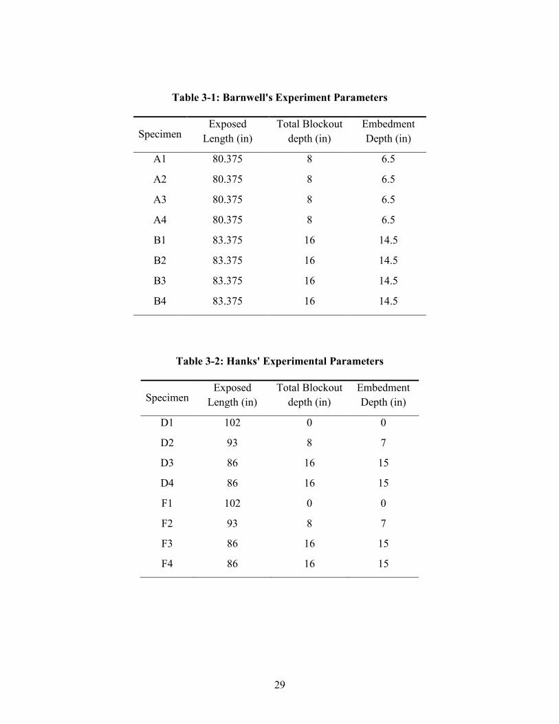
slab to the line of action of the actuator. Table 3-1 and Table 3-2 show the exposed length for
each of Barnwell’s and Hanks’ specimens respectively.
Two additional values are shown in Table 3-1 and Table 3-2; the total blockout depth and
the embedment depth. The total blockout depth was the full depth thickness of the main slab or
floor slab, which was poured on top of the foundation slab. The embedment depth was defined
as the distance from bottom of the base plate to the top of the blockout concrete slab. The
embedment depth was closely related to the total blockout depth, since the embedment depth was
equivalent to the depth of the blockout minus the layer of grout between the column base plate
and the base foundation concrete.
The values listed in Table 3-1 and Table 3-2 were used throughout this thesis. The
exposed length was investigated further for its influence on Tryon model in Section 4.2.1. The
embedment depth was used in several figures of rotational stiffness versus the embedment depth
throughout the thesis in order to evaluate the stiffness models.
The second step for generating hysteric plots was to calculate the total drift of the column.
The total drift of the column was determined by the total displacement of the column divided by
the exposed length of the column. The displacement of the column was calculated from the
string potentiometer measurements. The exposed length are the values listed in Table 3-1 and
Table 3-2. The total drift was then calculated for each time step.
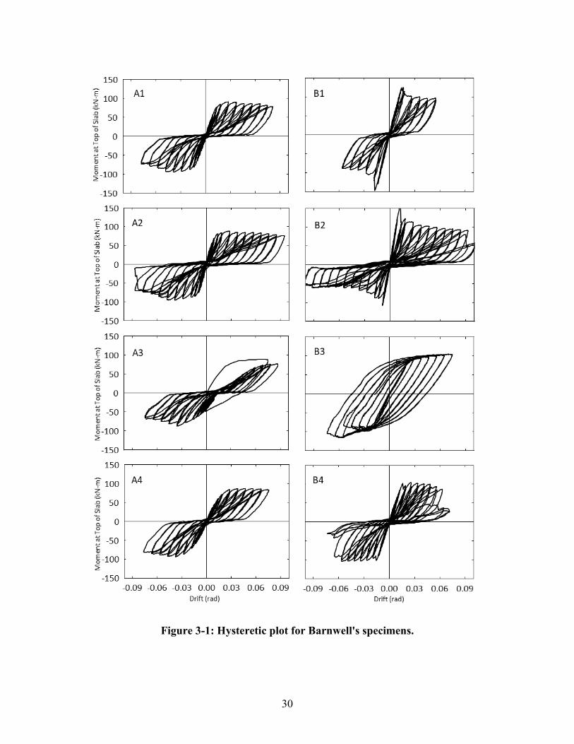
The final step was to generate the hysteretic plots. Figure 3-1 shows the hysteretic plots
for each of Barnwell’s specimens and Figures 3-2 and 3-3 show the hysteretic plots for each
Hanks’ testing series.
29
Table 3-1: Barnwell's Experiment Parameters
Specimen Exposed
Length (in) Total Blockout
depth (in) Embedment Depth (in)
A1 80.375 8 6.5
A2 80.375 8 6.5
A3 80.375 8 6.5
A4 80.375 8 6.5
B1 83.375 16 14.5
B2 83.375 16 14.5
B3 83.375 16 14.5
B4 83.375 16 14.5
Table 3-2: Hanks' Experimental Parameters
Specimen Exposed
Length (in) Total Blockout
depth (in) Embedment Depth (in)
D1 102 0 0
D2 93 8 7
D3 86 16 15
D4 86 16 15
F1 102 0 0
F2 93 8 7
F3 86 16 15
F4 86 16 15
30
Figure 3-1: Hysteretic plot for Barnwell's specimens.
31
Figure 3-2: Hysteretic plot for Hanks' D- series specimens.
Figure 3-3: Hysteretic plot for Hanks' F-series specimens.
32
Calculating Effective Rotational Stiffness
In order to calculate the effective rotational stiffness for each specimen, five steps were
implemented. These steps were: first, decompose the displacements of the column; second,
calculate the effective rotation of the connection; third, generate the backbone curves; fourth,
determine the intersection of the backbone with particular drift values; and fifth, find the slope of
the line representing the rotational stiffness.
The first step in calculating the rotational stiffness was to decompose the displacements of
the column. The total displacement of the column was made up of two components: the
displacement from the exposed column and the displacement from the base connection. The
total displacement was determined directly from the experimental testing, this was the same
value as was used in Section 3.2. The total displacement is defined as Equation (3-1). The
deflection from the column is simply the elastic deformation of a single column, which is
represented by the Equation (3-2). The parameters were F, the applied force; L, the distance
from the top of the slab to the line of action of the actuator or the exposed column length; E,
Young’s modulus; and I, the moment of inertia. The deformation from the connection was
determined from these two equations as shown in Equation (3-3). This decomposition is only
valid as long as the column stays in the elastic region; therefore, Young’s modulus stays
constant.
𝛿𝛿𝑓𝑓𝑓𝑓𝑓𝑓𝑏𝑏𝑏𝑏 = 𝛿𝛿𝑏𝑏𝑓𝑓𝑏𝑏𝑏𝑏𝑏𝑏𝑓𝑓 + 𝛿𝛿𝑏𝑏𝑓𝑓𝑓𝑓𝑓𝑓𝑏𝑏𝑏𝑏𝑓𝑓𝑓𝑓𝑓𝑓𝑓𝑓 (3-1)
𝛿𝛿𝑏𝑏𝑓𝑓𝑏𝑏𝑏𝑏𝑏𝑏𝑓𝑓 =𝐹𝐹𝐿𝐿3
3𝐸𝐸𝐸𝐸 (3-2)

33
𝛿𝛿𝑏𝑏𝑓𝑓𝑓𝑓𝑓𝑓𝑏𝑏𝑏𝑏𝑓𝑓𝑓𝑓𝑓𝑓𝑓𝑓 = 𝛿𝛿𝑓𝑓𝑓𝑓𝑓𝑓𝑏𝑏𝑏𝑏 −𝐹𝐹𝐿𝐿3
3𝐸𝐸𝐸𝐸 (3-3)
With the column displacement decomposed, the effective base rotation was determined by
using the displacement of column from only the connection, Equation (3-3). The effective
rotation was found by dividing the displacement due to the connection by the column exposed
length given in Tables 3-1 and 3-2.
The third step in the process of calculating the effective rotational stiffness was to generate
the backbone curve for each specimen. The backbone curve is the plot of the effective base
rotation, which was found in the previous step and plotting it against the moment at the top of the
slab, which was found in Section 3.2. The difference was that not all of the moment data was
used, only the maximum values per cycle or the backbone points.
The fourth step was to identify points corresponding to particular drift values. This was
done by finding the intersection of the backbone curve with a particular value of drift or the
effective base rotation. Values of 0.004 and 0.005 effective base rotation were used as
reasonable estimates. The 0.4 percent drift and the 0.5 percent drift were essentially averages of
the higher stiffness at lower percentages and the reduced stiffness at later percentages. The drift
values chosen were the same for all specimens. The drift was linearly interpolated from the
available data points of the backbone curve.
The final step was to find the slope of the line between the two drift points. This slope
value was the estimated effective rotational stiffness. A typical plot is shown in Figure 3-4. The
A2 line represents the backbone curve and the two dashed lines are the estimated effective
rotational stiffness for two assumed drift values.
34
Figure 3-4: Specimen A2 rotational stiffness calculation.
Results
Figure 3-5 through Figure 3-20 show the plots for each specimen in the Barnwell’s and
Hanks’ test with the moment at the top of the slab versus the effective base rotation. Barnwell’s
series A are presented in Figure 3-5 through Figure 3-8 and Figure 3-9 through Figure 3-12 are
for Barnwell’s series B. Figure 3-13 through Figure 3-16 are for Hanks’ series D and Hanks’
series F is as shown in Figure 3-17 through Figure 3-20.
The rotational stiffness values were calculated based on the slope of the line through the
0.5 percent story drift points in Figure 3-5 through Figure 3-20. The rotational stiffness values
obtained are listed in Table 3-3 for Barnwell’s specimens and in Table 3-4 for Hanks’ specimens.
Note that in Table 3-3 specimen B3 and B4 did not have a value for the rotational stiffness. This
was because the general method was not reliable for these specimens since they had flexible
columns and limited connection deformation before column yielding. Additionally, the method
for decomposing the drift may not be valid in these cases.
35
Barnwell’s A Series
Figure 3-5: Specimen A1 moment at top of slab versus effective base rotation. (W8x35 Strong – 6.5 inches embedment depth).
Figure 3-6: Specimen A2 moment at top of slab versus effective base rotation (W8x48 Strong – 6.5 inches embedment depth).
36
Figure 3-7: Specimen A3 moment at top of slab versus effective base rotation (W8x35 Weak – 6.5 inches embedment depth).
Figure 3-8: Specimen A4 moment at top of slab versus effective base rotation (W8x48 Weak – 6.5 inches embedment depth).
37
Barnwell B Series
Figure 3-9: Specimen B1 moment at top of slab versus effective base rotation (W8x35 Strong – 14.5 inches embedment depth).
Figure 3-10: Specimen B2 moment at top of slab versus effective base rotation (W8x48 Strong – 14.5 inches embedment depth).
38
Figure 3-11: Specimen B3 moment at top of slab versus effective base rotation (W8x35 Weak – 14.5 inches embedment depth).
Figure 3-12: Specimen B4 moment at top of slab versus effective base rotation (W8x48 Weak – 14.5 inches embedment depth).
39
Hanks D Series
Figure 3-13: Specimen D1 moment at top of slab versus effective base rotation (W14x35 Strong – 0 inches embedment depth).
Figure 3-14: Specimen D2 moment at top of slab versus effective base rotation (W14x35 Strong – 7 inches embedment depth).
40
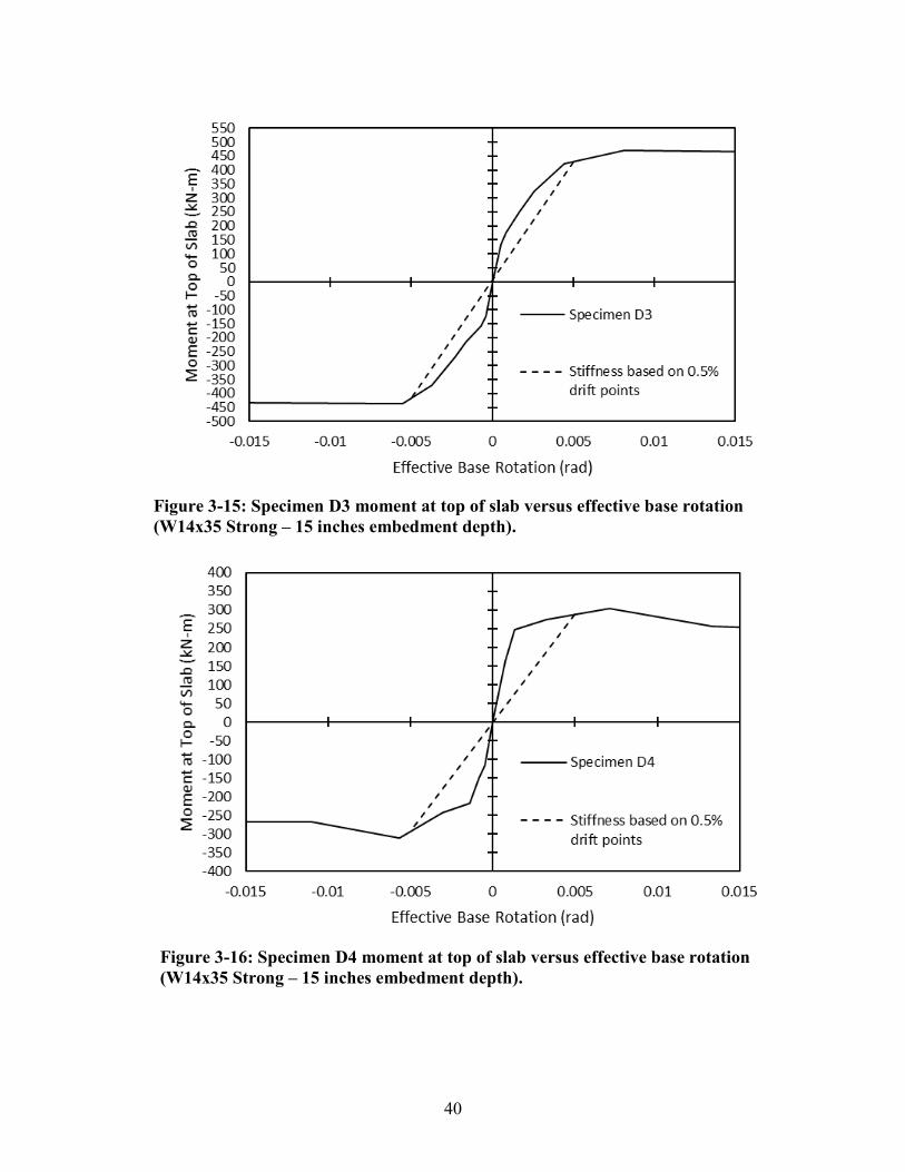
Figure 3-15: Specimen D3 moment at top of slab versus effective base rotation (W14x35 Strong – 15 inches embedment depth).
Figure 3-16: Specimen D4 moment at top of slab versus effective base rotation (W14x35 Strong – 15 inches embedment depth).
41
Hanks F Series
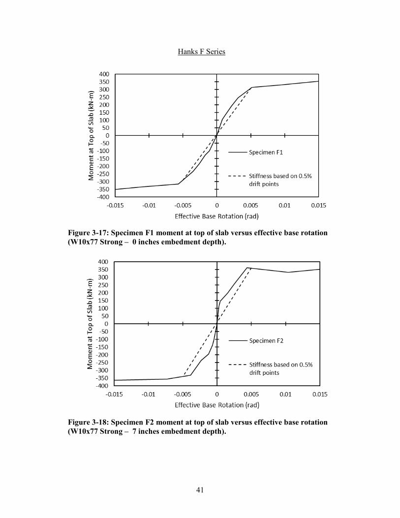
Figure 3-17: Specimen F1 moment at top of slab versus effective base rotation (W10x77 Strong – 0 inches embedment depth).
Figure 3-18: Specimen F2 moment at top of slab versus effective base rotation (W10x77 Strong – 7 inches embedment depth).
42
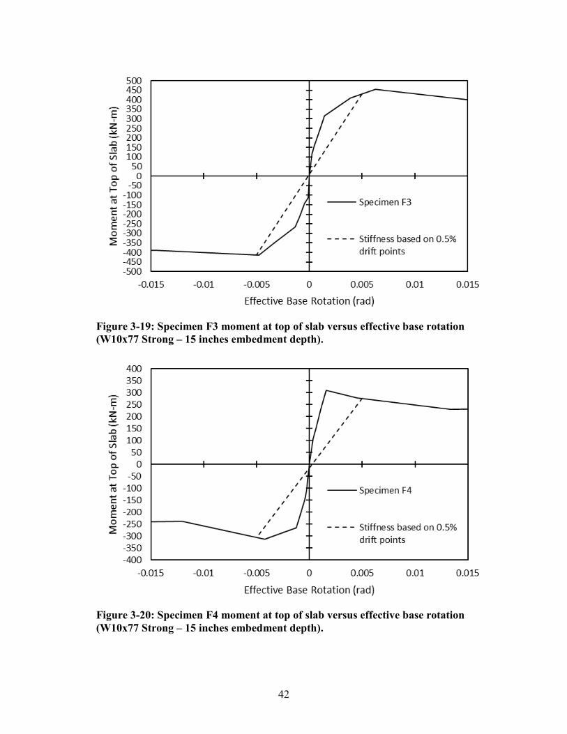
Figure 3-19: Specimen F3 moment at top of slab versus effective base rotation (W10x77 Strong – 15 inches embedment depth).
Figure 3-20: Specimen F4 moment at top of slab versus effective base rotation (W10x77 Strong – 15 inches embedment depth).

43
Table 3-3: Rotational Stiffness Values from Barnwell's Experiments
Specimens Rotational Stiffness
@ 0.5% Drift (kN-m/rad) Rotational Stiffness
@ 0.4% Drift (kN-m/rad) A1 11567 12318 A2 12806 14212
A3 9470 10241 A4 11027 12353 B1 23587 24429
B2 26599 31392 B3 N/A N/A
B4 N/A N/A
Table 3-4: Rotational Stiffness Values from Hanks’ Experiments
Specimens Rotational Stiffness
@ 0.5% Drift (kN-m/rad) Rotational Stiffness
@ 0.4% Drift (kN-m/rad) D1 55145 59872
D2 68074 75914
D3 84606 97305
D4 58121 68416
F1 59811 65850
F2 69844 83928
F3 84239 98660
F4 58193 74185
Summary
Data reduction was necessary in order to ensure that similar values were being compared.
The values determined in this section were the values that were used for analysis in the rest of
the thesis. Although the rotational stiffness values seen in this section were approximations for
the 0.5 percent story drift, any value of percent drift can be calculated and used in a similar

44
manner. The 0.5 percent story drift was chosen, because it was an average of the higher stiffness
at lower story drift values and the lower stiffness at higher story drift values. However, as shown
in Figure 3-5 through Figure 3-20, the 0.5 percent story drift was not always the best
approximation.
The values presented in this section were slightly different from those that were presented
in Tryon’s or Hanks’ theses, Barnwell did not present rotational stiffness values in his thesis.
The values in Table 3-3 were about two times smaller than the values reported by Tryon for
Barnwell’s testing and the valued in Table 3-4 were also smaller than those reported in Hanks’
thesis. Values from Table 3-4 were between 15% but less than 50% of Hanks’ reported values,
because both Hanks and Tryon used different percent story drifts than the value used in this
thesis. In addition, the stiffness was calculated with small differences in the embedment depth
and exposed length.

45
4 MODIFIED TRYON MODEL
Introduction
With the data reduction complete, the experimental data was compared with the results
from Tryon’s model. Tryon’s model was investigated in order to determine the parameters that
were significant. Each parameter was either added directly without modifications into a new
version of Tryon’s model or the parameter were altered for a better fit of the data before being
added into the model.
The main parameters in Tryon’s continuum model are embedment depth, exposed length,
flange effective width, modulus of subgrade reaction, and base plate rotational stiffness, ks, as
stated in Section 2.2.4. The embedment depth was discussed in Section 3.2. The exposed length
was introduced in Section 3.2 and is discussed further in Section 4.2.1. The flange effective
width and modulus of subgrade reaction are influential components to the rotational stiffness
equations and are discussed in Sections 4.2.2 and 4.2.3, respectively.
Results are shown in Section 4.3 for the relationship between the rotational stiffness that
was determined in Section 3.4 and the model with the modified parameters.

46
Influence of Various Parameters in Tryon’s Model
4.2.1 Effects of Exposed Lengths
The sensitivity of the resulting model for a single exposed length, when the column size
and orientation match, was investigated. Since Barnwell’s specimens had two different exposed
lengths, the sensitivity of the model to this parameter was investigated. For Barnwell’s tests,
there was an exposed length of 80.375 inches for specimens with an 8-inch blockout depth and
83.375 inches for the specimens with a 16-inch blockout depth. It was believed that the 3-inch
difference would not cause a significant change in the response of Tryon’s model. Figure 4-1
shows the difference in the rotational stiffness as predicted by Tryon’s model for the two
different exposed lengths from Barnwell’s data if all other parameters were held constant. The
small difference in exposed length did not have much impact on the results from Tryon’s model.
Thus, an exposed length of 83.375 inches was assumed for comparison with Tryon’s model in
other parameter studies. The exposed length of 83.375 inches was used in Tryon’s model to
calculate the moment, which was in turn used to estimate the total rotation and displacement of
the column.
Hanks’, specimen D2 and F2 had an exposed length of 93 inches and specimen D3, D4,
F3, and F4 had an exposed length of 86 inches. Specimens D1 and F1 did not have a blockout,
so their exposed length was 102 inches. Even though there was a greater difference between the
three exposed lengths for Hanks’ data, it was still believed that the difference in exposed length
was small enough that there would not be significant difference in the response of Tryon’s
model. Figure 4-2 shows the comparison of the three lengths with similar parameter
assumptions. Since there was an insignificant difference in the response of the model, a single
value of 86 inches was assumed for the exposed length for Hanks’ experiments in other

47
parameter studies. The single value chosen for Hanks’ data as well as Barnwell’s data would be
used to generate the curves shown throughout the remainder of this thesis. The exposed length
was an important parameter in calculating the moment induced on the specimen.
Figure 4-1: Exposed length comparison for Barnwell’s experiments (ko = 150kip/in3).
Figure 4-2: Exposed length comparison for Hanks’ experiments (ko = 150kip/in3).

48
4.2.2 Effects of Flange Effective Width
A further assumption that was evaluated for Tryon’s model was flange effective width,
which Tryon called flange duality and the effective width of the column. As was discussed in
Section 2.2.4, Tryon assumed that both flanges would act in resisting against the blockout
concrete. In order to check the flange effective width, curves were generated using Tryon’s
model, one with the assumption of both flanges resisting and another accounting for only one of
the flanges resisting against the blockout concrete. Barnwell’s experimental data was then
compared to the two curves to determine the best fit. The affected parameter was mainly the
spring rotational stiffness; however, Tryon’s calculations for the modulus of subgrade reaction
was also affected.
The flange effective width was then removed from Equation (2-1) and Equation (2-2)
which became Equation (4-1) and Equation (4-2), respectively. Notice that Equation (4-2) does
not change since this was for the weak orientation of the column and therefore the two flanges
were not acting in resistance. The variable k in theses equations represents the concrete stiffness
and was determined by the modulus of subgrade reaction multiplied by the depth of the flanges if
strong axis and the depth of the column if the weak axis was used.
𝑘𝑘𝑠𝑠 =𝑘𝑘𝑑𝑑3
24�𝐸𝐸𝑓𝑓𝑓𝑓𝑓𝑓𝑓𝑓𝑓𝑓𝑓𝑓𝑓𝑓𝐸𝐸𝑏𝑏𝑏𝑏𝑓𝑓𝑏𝑏𝑏𝑏𝑓𝑓𝑏𝑏𝑓𝑓
+ 1� (4-1)
𝑘𝑘𝑠𝑠 =𝑘𝑘𝑏𝑏𝑓𝑓3
24�𝐸𝐸𝑓𝑓𝑓𝑓𝑓𝑓𝑓𝑓𝑓𝑓𝑓𝑓𝑓𝑓𝐸𝐸𝑏𝑏𝑏𝑏𝑓𝑓𝑏𝑏𝑏𝑏𝑓𝑓𝑏𝑏𝑓𝑓
+ 1� (4-2)
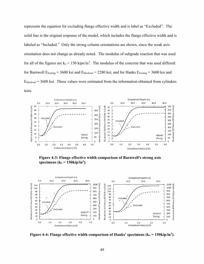
The results of the flange effective width analysis are shown in Figure 4-3 for Barnwell’s
strong axis specimens and in Figure 4-4 for Hanks’ specimens. The dashed line in these figures
49
represents the equation for excluding flange effective width and is label as “Excluded”. The
solid line is the original response of the model, which includes the flange effective width and is
labeled as “Included.” Only the strong column orientations are shown, since the weak axis
orientation does not change as already noted. The modulus of subgrade reaction that was used
for all of the figures are ko = 150 kips/in3. The modulus of the concrete that was used differed:
for Barnwell Efooting = 3600 ksi and Eblockout = 2280 ksi; and for Hanks Efooting = 3600 ksi and
Eblockout = 3600 ksi. These values were estimated from the information obtained from cylinders
tests.
Figure 4-3: Flange effective width comparison of Barnwell's strong axis specimens (ko = 150kip/in3).
Figure 4-4: Flange effective width comparison of Hanks' specimens (ko = 150kip/in3).
50
Figure 4-3 shows that Barnwell’s data fits better with flange effective width excluded;
however, Figure 4-4 suggests that Hanks’ data may fit slightly better with flange effective width
included. Although there are too few points to say definitively which way is better. However,
the flange effective width was removed for later parameter investigation, since there appeared to
not be an extreme change between the two curves and Hanks’ data in some cases seems to fit
better with the excluded flange effective width.
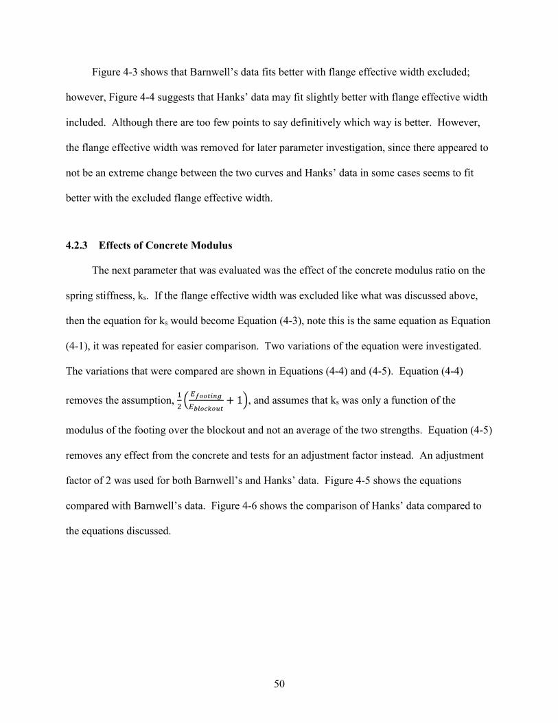
4.2.3 Effects of Concrete Modulus
The next parameter that was evaluated was the effect of the concrete modulus ratio on the
spring stiffness, ks. If the flange effective width was excluded like what was discussed above,
then the equation for ks would become Equation (4-3), note this is the same equation as Equation
(4-1), it was repeated for easier comparison. Two variations of the equation were investigated.
The variations that were compared are shown in Equations (4-4) and (4-5). Equation (4-4)
removes the assumption, 12� 𝐸𝐸𝑓𝑓𝑓𝑓𝑓𝑓𝑓𝑓𝑓𝑓𝑓𝑓𝑓𝑓𝐸𝐸𝑏𝑏𝑏𝑏𝑓𝑓𝑏𝑏𝑏𝑏𝑓𝑓𝑏𝑏𝑓𝑓
+ 1�, and assumes that ks was only a function of the
modulus of the footing over the blockout and not an average of the two strengths. Equation (4-5)
removes any effect from the concrete and tests for an adjustment factor instead. An adjustment
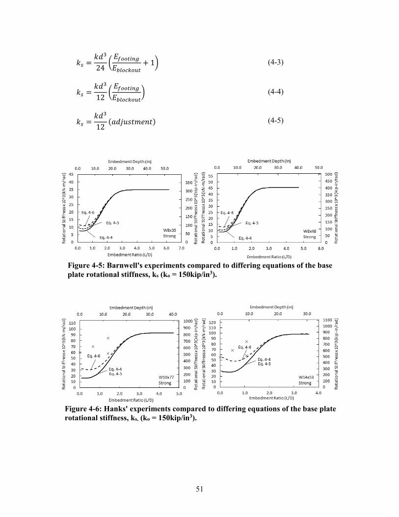
factor of 2 was used for both Barnwell’s and Hanks’ data. Figure 4-5 shows the equations
compared with Barnwell’s data. Figure 4-6 shows the comparison of Hanks’ data compared to
the equations discussed.
51
Figure 4-5: Barnwell's experiments compared to differing equations of the base plate rotational stiffness, ks (ko = 150kip/in3).
Figure 4-6: Hanks' experiments compared to differing equations of the base plate rotational stiffness, ks, (ko = 150kip/in3).
𝑘𝑘𝑠𝑠 =𝑘𝑘𝑑𝑑3
24�𝐸𝐸𝑓𝑓𝑓𝑓𝑓𝑓𝑓𝑓𝑓𝑓𝑓𝑓𝑓𝑓𝐸𝐸𝑏𝑏𝑏𝑏𝑓𝑓𝑏𝑏𝑏𝑏𝑓𝑓𝑏𝑏𝑓𝑓
+ 1� (4-3)
𝑘𝑘𝑠𝑠 =𝑘𝑘𝑑𝑑3
12�𝐸𝐸𝑓𝑓𝑓𝑓𝑓𝑓𝑓𝑓𝑓𝑓𝑓𝑓𝑓𝑓𝐸𝐸𝑏𝑏𝑏𝑏𝑓𝑓𝑏𝑏𝑏𝑏𝑓𝑓𝑏𝑏𝑓𝑓
� (4-4)
𝑘𝑘𝑠𝑠 =𝑘𝑘𝑑𝑑3
12(𝑎𝑎𝑑𝑑𝑎𝑎𝑎𝑎𝑎𝑎𝑡𝑡𝑎𝑎𝑎𝑎𝑎𝑎𝑡𝑡) (4-5)

52
Figure 4-5 shows that Barnwell’s data fits fairly well with any of the equations, since
Barnwell did not test any exposed base connection columns. Figure 4-6 suggests that a different
modulus of subgrade reaction may be required or an additional change in a parameter. These
equations will be evaluated further in the Section 4.3 on combined effects.
Combined Effects
4.3.1 Barnwell’s Data
Figure 4-7 shows the relationship between Barnwell’s data and Tryon’s model. Tryon’s
model was updated with the assumptions that were described in the preceding subsections. The
curves were generated using Equation (4-4) for two different shapes in the strong and weak axis
direction, with a variety of values for the modulus of subgrade reaction, 100 kip/in3, 150 kip/in3,
and 200 kip/in3. The “xs” in the figure correlate to the stiffness calculated at 0.5 percent story
drift. The results show that Tryon’s model is sensitive to the modulus of subgrade reaction
value assumed, as well as the way the stiffness was calculated for the specimen. The best fit for
this strong axis loading is with ko = 150 kip/in3.
The best fit values for Tryon’s model for the weak axis orientation was a little more
difficult to determine since only one data point for each shape and orientation combination was
available. The best approximation for ko for the weak axis loading is 200 kip/in3. The lack of
experimental results was due to some errors during testing that did not allow for the actual
stiffness to be calculated for comparison.
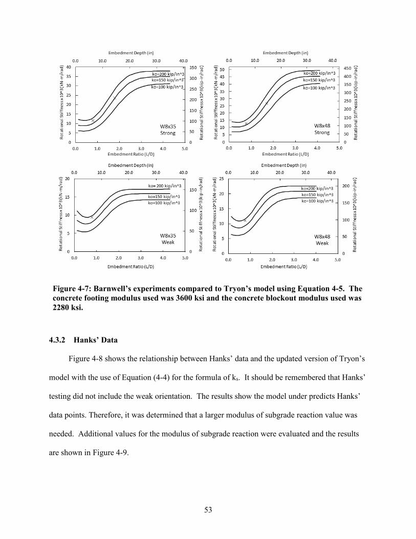
53
Figure 4-7: Barnwell’s experiments compared to Tryon’s model using Equation 4-5. The concrete footing modulus used was 3600 ksi and the concrete blockout modulus used was 2280 ksi.
4.3.2 Hanks’ Data
Figure 4-8 shows the relationship between Hanks’ data and the updated version of Tryon’s
model with the use of Equation (4-4) for the formula of ks. It should be remembered that Hanks’
testing did not include the weak orientation. The results show the model under predicts Hanks’
data points. Therefore, it was determined that a larger modulus of subgrade reaction value was
needed. Additional values for the modulus of subgrade reaction were evaluated and the results
are shown in Figure 4-9.
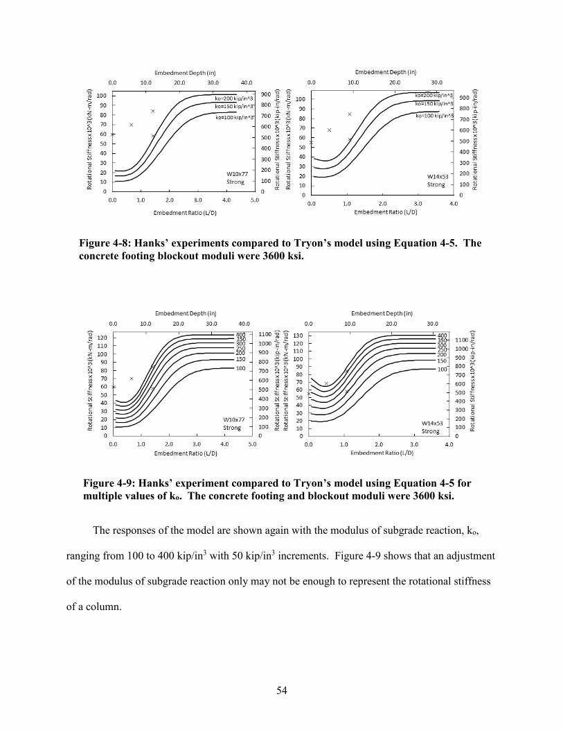
54
Figure 4-8: Hanks’ experiments compared to Tryon’s model using Equation 4-5. The concrete footing blockout moduli were 3600 ksi.
Figure 4-9: Hanks’ experiment compared to Tryon’s model using Equation 4-5 for multiple values of ko. The concrete footing and blockout moduli were 3600 ksi.
The responses of the model are shown again with the modulus of subgrade reaction, ko,
ranging from 100 to 400 kip/in3 with 50 kip/in3 increments. Figure 4-9 shows that an adjustment
of the modulus of subgrade reaction only may not be enough to represent the rotational stiffness
of a column.
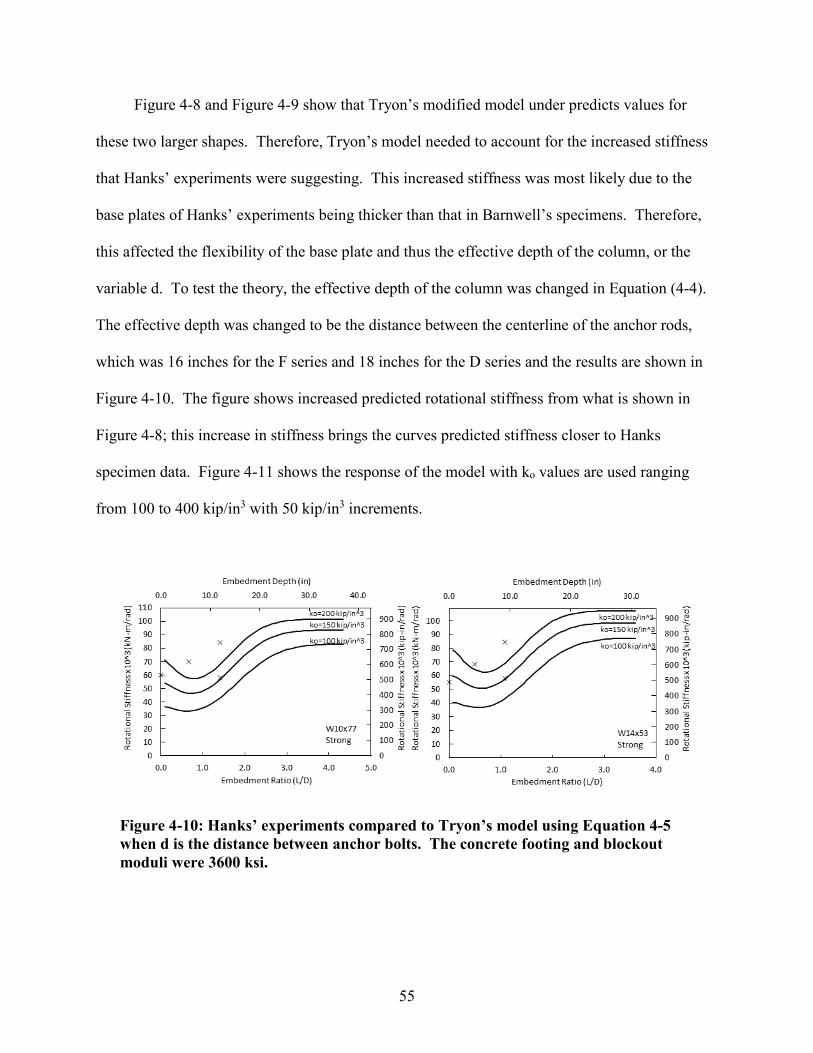
55
Figure 4-8 and Figure 4-9 show that Tryon’s modified model under predicts values for
these two larger shapes. Therefore, Tryon’s model needed to account for the increased stiffness
that Hanks’ experiments were suggesting. This increased stiffness was most likely due to the
base plates of Hanks’ experiments being thicker than that in Barnwell’s specimens. Therefore,
this affected the flexibility of the base plate and thus the effective depth of the column, or the
variable d. To test the theory, the effective depth of the column was changed in Equation (4-4).
The effective depth was changed to be the distance between the centerline of the anchor rods,
which was 16 inches for the F series and 18 inches for the D series and the results are shown in
Figure 4-10. The figure shows increased predicted rotational stiffness from what is shown in
Figure 4-8; this increase in stiffness brings the curves predicted stiffness closer to Hanks
specimen data. Figure 4-11 shows the response of the model with ko values are used ranging
from 100 to 400 kip/in3 with 50 kip/in3 increments.
Figure 4-10: Hanks’ experiments compared to Tryon’s model using Equation 4-5 when d is the distance between anchor bolts. The concrete footing and blockout moduli were 3600 ksi.
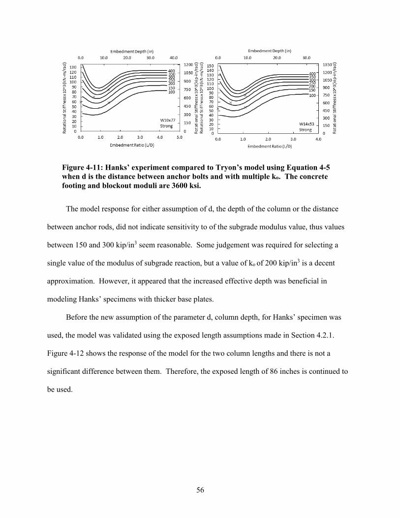
56
Figure 4-11: Hanks’ experiment compared to Tryon’s model using Equation 4-5 when d is the distance between anchor bolts and with multiple ko. The concrete footing and blockout moduli are 3600 ksi.
The model response for either assumption of d, the depth of the column or the distance
between anchor rods, did not indicate sensitivity to of the subgrade modulus value, thus values
between 150 and 300 kip/in3 seem reasonable. Some judgement was required for selecting a
single value of the modulus of subgrade reaction, but a value of ko of 200 kip/in3 is a decent
approximation. However, it appeared that the increased effective depth was beneficial in
modeling Hanks’ specimens with thicker base plates.
Before the new assumption of the parameter d, column depth, for Hanks’ specimen was
used, the model was validated using the exposed length assumptions made in Section 4.2.1.
Figure 4-12 shows the response of the model for the two column lengths and there is not a
significant difference between them. Therefore, the exposed length of 86 inches is continued to
be used.

57
Figure 4-12: Exposed length comparison for Hanks’ experiments when d is the distance between anchor bolts. d = 16 inches for W10 and d = 18 inches for W14 (ko = 150 kip/in3).
4.3.3 Direct Comparison
Figure 4-13 shows the direct comparison of Tryon’s original model to the modified model
with Barnwell’s specimens represented with “xs”. A value for the modulus of subgrade reaction
of 150 kip/in3 was used for modeling as was suggested in Section 4.3.1. It can be seen that for
the lower embedment there is not a lot of difference in the model, but for the deeper embedment
there is a greater change. A similar comparison is shown for Hanks data in Figure 4-14. Again,
a direct comparison of the original model and the modified model. Hanks’ specimens are shown
with “xs”. A modulus of subgrade reaction of 200 kip/in3 was used as suggested in Section
4.3.2. There is not as close a solution for Hanks’ specimens; however, Hanks’ results are fairly
close to the predicted rotational stiffnesses.
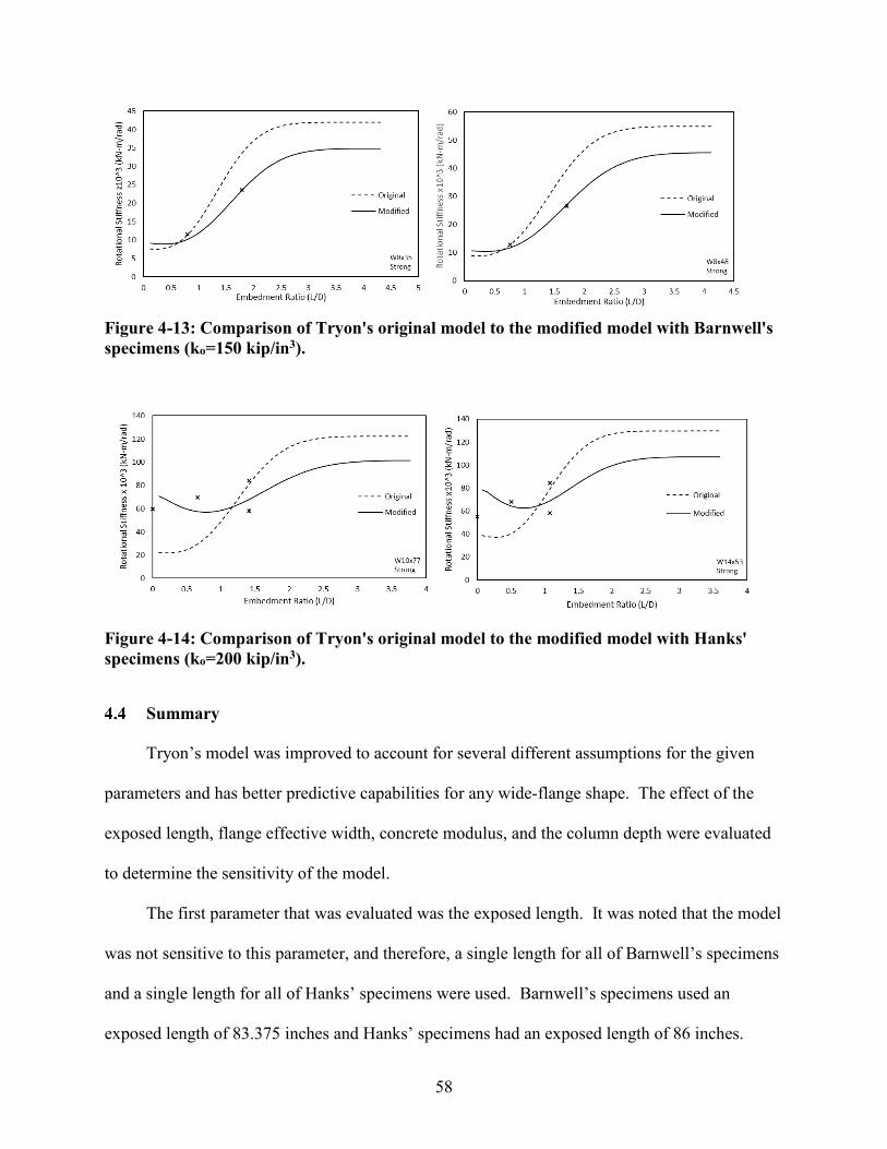
58
Figure 4-13: Comparison of Tryon's original model to the modified model with Barnwell's specimens (ko=150 kip/in3).
Figure 4-14: Comparison of Tryon's original model to the modified model with Hanks' specimens (ko=200 kip/in3).
Summary
Tryon’s model was improved to account for several different assumptions for the given
parameters and has better predictive capabilities for any wide-flange shape. The effect of the
exposed length, flange effective width, concrete modulus, and the column depth were evaluated
to determine the sensitivity of the model.
The first parameter that was evaluated was the exposed length. It was noted that the model
was not sensitive to this parameter, and therefore, a single length for all of Barnwell’s specimens
and a single length for all of Hanks’ specimens were used. Barnwell’s specimens used an
exposed length of 83.375 inches and Hanks’ specimens had an exposed length of 86 inches.
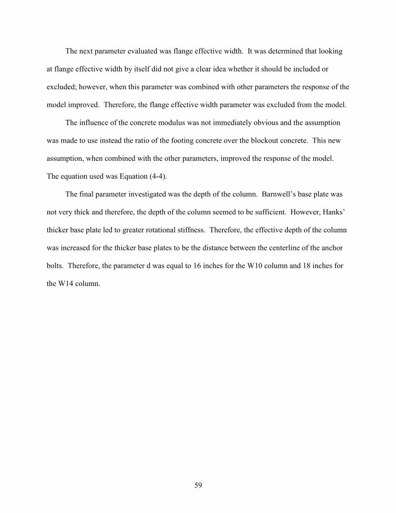
59
The next parameter evaluated was flange effective width. It was determined that looking
at flange effective width by itself did not give a clear idea whether it should be included or
excluded; however, when this parameter was combined with other parameters the response of the
model improved. Therefore, the flange effective width parameter was excluded from the model.
The influence of the concrete modulus was not immediately obvious and the assumption
was made to use instead the ratio of the footing concrete over the blockout concrete. This new
assumption, when combined with the other parameters, improved the response of the model.
The equation used was Equation (4-4).
The final parameter investigated was the depth of the column. Barnwell’s base plate was
not very thick and therefore, the depth of the column seemed to be sufficient. However, Hanks’
thicker base plate led to greater rotational stiffness. Therefore, the effective depth of the column
was increased for the thicker base plates to be the distance between the centerline of the anchor
bolts. Therefore, the parameter d was equal to 16 inches for the W10 column and 18 inches for
the W14 column.

60
5 SYSTEM LEVEL SENSITIVITY
Introduction
In Tryon’s model the rotational stiffness, β, was dependent upon the value chosen for the
modulus of subgrade reaction, ko. However, determining an appropriate value for the modulus
of subgrade reaction is a challenge. It was, therefore, determined to study the sensitivity of the
total stiffness to the rotational stiffness, β, and determine how accurate β must be in order to
obtain reasonable values for the total stiffness. The sensitivity analysis was done by comparing
the system stiffness to the rotational stiffness, β, for several values of the modulus of subgrade
reaction. A moment frame with partially fixed base columns was used in this study.
Method
5.2.1 Sensitivity of Total Stiffness as Modulus of Subgrade Reaction Changes
The total stiffness of a column was investigated to determine its sensitivity to β as ko was
changed. This was done by determining the stiffness of the column and base connection
separately. Equation (5-1) is the flexural stiffness of a single cantilever column, which depends
on the modulus of elasticity, the moment of inertia, and the exposed length of the column. The
stiffness of the embedment depth was determined by Equation (5-2). This was the stiffness
provided by a rotational spring at the top of the slab. The rotational stiffness at the top of the
slab provided by the embedment, β, was determined by using Hetényi’s beam equations and the
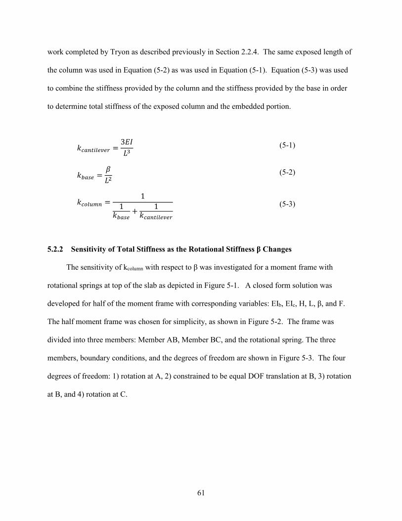
61
work completed by Tryon as described previously in Section 2.2.4. The same exposed length of
the column was used in Equation (5-2) as was used in Equation (5-1). Equation (5-3) was used
to combine the stiffness provided by the column and the stiffness provided by the base in order
to determine total stiffness of the exposed column and the embedded portion.
𝑘𝑘𝑏𝑏𝑏𝑏𝑓𝑓𝑓𝑓𝑓𝑓𝑏𝑏𝑏𝑏𝑒𝑒𝑏𝑏𝑏𝑏 =3𝐸𝐸𝐸𝐸𝐿𝐿3
(5-1)
𝑘𝑘𝑏𝑏𝑏𝑏𝑠𝑠𝑏𝑏 =𝛽𝛽𝐿𝐿2
(5-2)
𝑘𝑘𝑏𝑏𝑓𝑓𝑏𝑏𝑏𝑏𝑏𝑏𝑓𝑓 =1
1𝑘𝑘𝑏𝑏𝑏𝑏𝑠𝑠𝑏𝑏
+ 1𝑘𝑘𝑏𝑏𝑏𝑏𝑓𝑓𝑓𝑓𝑓𝑓𝑏𝑏𝑏𝑏𝑒𝑒𝑏𝑏𝑏𝑏
(5-3)
5.2.2 Sensitivity of Total Stiffness as the Rotational Stiffness β Changes
The sensitivity of kcolumn with respect to β was investigated for a moment frame with
rotational springs at top of the slab as depicted in Figure 5-1. A closed form solution was
developed for half of the moment frame with corresponding variables: EIb, EIc, H, L, β, and F.
The half moment frame was chosen for simplicity, as shown in Figure 5-2. The frame was
divided into three members: Member AB, Member BC, and the rotational spring. The three
members, boundary conditions, and the degrees of freedom are shown in Figure 5-3. The four
degrees of freedom: 1) rotation at A, 2) constrained to be equal DOF translation at B, 3) rotation
at B, and 4) rotation at C.

62
Figure 5-1: Full moment frame and system parameters with partial fixity denoted at the top of the slab.
Figure 5-2: Half the moment frame and system parameters for the system analyzed with partial fixity denoted at the top of the slab.
Figure 5-3: The four degrees of freedom and nodes for the half moment frame.
F
F
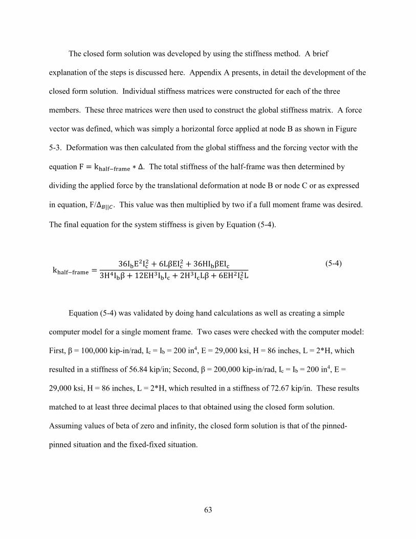
63
The closed form solution was developed by using the stiffness method. A brief
explanation of the steps is discussed here. Appendix A presents, in detail the development of the
closed form solution. Individual stiffness matrices were constructed for each of the three
members. These three matrices were then used to construct the global stiffness matrix. A force
vector was defined, which was simply a horizontal force applied at node B as shown in Figure
5-3. Deformation was then calculated from the global stiffness and the forcing vector with the
equation F = khalf−frame ∗ Δ. The total stiffness of the half-frame was then determined by
dividing the applied force by the translational deformation at node B or node C or as expressed
in equation, F/∆𝐻𝐻||𝐶𝐶 . This value was then multiplied by two if a full moment frame was desired.
The final equation for the system stiffness is given by Equation (5-4).
Equation (5-4) was validated by doing hand calculations as well as creating a simple
computer model for a single moment frame. Two cases were checked with the computer model:
First, β = 100,000 kip-in/rad, Ic = Ib = 200 in4, E = 29,000 ksi, H = 86 inches, L = 2*H, which
resulted in a stiffness of 56.84 kip/in; Second, β = 200,000 kip-in/rad, Ic = Ib = 200 in4, E =
29,000 ksi, H = 86 inches, L = 2*H, which resulted in a stiffness of 72.67 kip/in. These results
matched to at least three decimal places to that obtained using the closed form solution.
Assuming values of beta of zero and infinity, the closed form solution is that of the pinned-
pinned situation and the fixed-fixed situation.
khalf−frame =36IbE2Ic2 + 6LβEIc2 + 36HIbβEIc
3H4Ibβ + 12EH3IbIc + 2H3IcLβ + 6EH2Ic2L
(5-4)
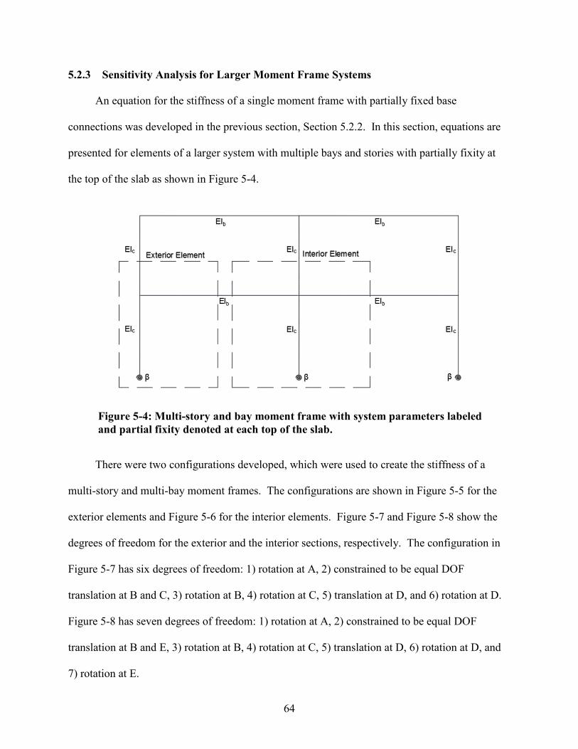
64
5.2.3 Sensitivity Analysis for Larger Moment Frame Systems
An equation for the stiffness of a single moment frame with partially fixed base
connections was developed in the previous section, Section 5.2.2. In this section, equations are
presented for elements of a larger system with multiple bays and stories with partially fixity at
the top of the slab as shown in Figure 5-4.
Figure 5-4: Multi-story and bay moment frame with system parameters labeled and partial fixity denoted at each top of the slab.
There were two configurations developed, which were used to create the stiffness of a
multi-story and multi-bay moment frames. The configurations are shown in Figure 5-5 for the
exterior elements and Figure 5-6 for the interior elements. Figure 5-7 and Figure 5-8 show the
degrees of freedom for the exterior and the interior sections, respectively. The configuration in
Figure 5-7 has six degrees of freedom: 1) rotation at A, 2) constrained to be equal DOF
translation at B and C, 3) rotation at B, 4) rotation at C, 5) translation at D, and 6) rotation at D.
Figure 5-8 has seven degrees of freedom: 1) rotation at A, 2) constrained to be equal DOF
translation at B and E, 3) rotation at B, 4) rotation at C, 5) translation at D, 6) rotation at D, and
7) rotation at E.
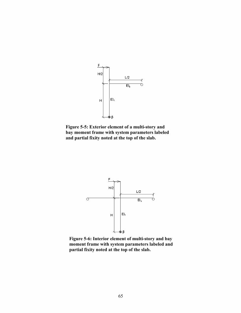
65
Figure 5-5: Exterior element of a multi-story and bay moment frame with system parameters labeled and partial fixity noted at the top of the slab.
Figure 5-6: Interior element of multi-story and bay moment frame with system parameters labeled and partial fixity noted at the top of the slab.
F
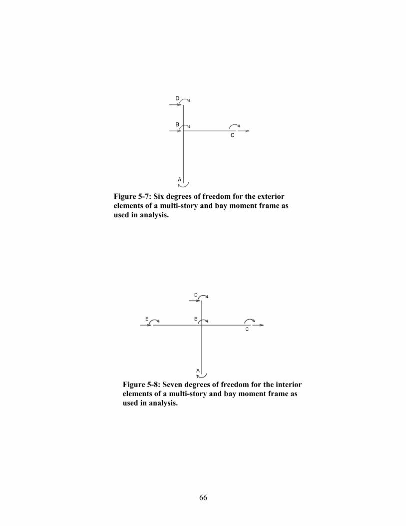
66
Figure 5-7: Six degrees of freedom for the exterior elements of a multi-story and bay moment frame as used in analysis.
Figure 5-8: Seven degrees of freedom for the interior elements of a multi-story and bay moment frame as used in analysis.
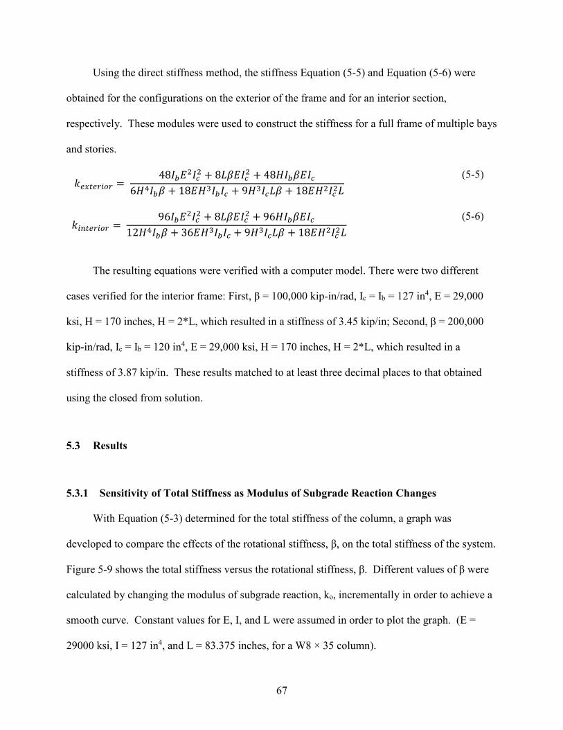
67
Using the direct stiffness method, the stiffness Equation (5-5) and Equation (5-6) were
obtained for the configurations on the exterior of the frame and for an interior section,
respectively. These modules were used to construct the stiffness for a full frame of multiple bays
and stories.
𝑘𝑘𝑏𝑏𝑚𝑚𝑓𝑓𝑏𝑏𝑏𝑏𝑓𝑓𝑓𝑓𝑏𝑏 = 48𝐸𝐸𝑏𝑏𝐸𝐸2𝐸𝐸𝑏𝑏2 + 8𝐿𝐿𝛽𝛽𝐸𝐸𝐸𝐸𝑏𝑏2 + 48𝐻𝐻𝐸𝐸𝑏𝑏𝛽𝛽𝐸𝐸𝐸𝐸𝑏𝑏
6𝐻𝐻4𝐸𝐸𝑏𝑏𝛽𝛽 + 18𝐸𝐸𝐻𝐻3𝐸𝐸𝑏𝑏𝐸𝐸𝑏𝑏 + 9𝐻𝐻3𝐸𝐸𝑏𝑏𝐿𝐿𝛽𝛽 + 18𝐸𝐸𝐻𝐻2𝐸𝐸𝑏𝑏2𝐿𝐿
(5-5)
𝑘𝑘𝑓𝑓𝑓𝑓𝑓𝑓𝑏𝑏𝑏𝑏𝑓𝑓𝑓𝑓𝑏𝑏 = 96𝐸𝐸𝑏𝑏𝐸𝐸2𝐸𝐸𝑏𝑏2 + 8𝐿𝐿𝛽𝛽𝐸𝐸𝐸𝐸𝑏𝑏2 + 96𝐻𝐻𝐸𝐸𝑏𝑏𝛽𝛽𝐸𝐸𝐸𝐸𝑏𝑏
12𝐻𝐻4𝐸𝐸𝑏𝑏𝛽𝛽 + 36𝐸𝐸𝐻𝐻3𝐸𝐸𝑏𝑏𝐸𝐸𝑏𝑏 + 9𝐻𝐻3𝐸𝐸𝑏𝑏𝐿𝐿𝛽𝛽 + 18𝐸𝐸𝐻𝐻2𝐸𝐸𝑏𝑏2𝐿𝐿
(5-6)
The resulting equations were verified with a computer model. There were two different
cases verified for the interior frame: First, β = 100,000 kip-in/rad, Ic = Ib = 127 in4, E = 29,000
ksi, H = 170 inches, H = 2*L, which resulted in a stiffness of 3.45 kip/in; Second, β = 200,000
kip-in/rad, Ic = Ib = 120 in4, E = 29,000 ksi, H = 170 inches, H = 2*L, which resulted in a
stiffness of 3.87 kip/in. These results matched to at least three decimal places to that obtained
using the closed from solution.
Results
5.3.1 Sensitivity of Total Stiffness as Modulus of Subgrade Reaction Changes
With Equation (5-3) determined for the total stiffness of the column, a graph was
developed to compare the effects of the rotational stiffness, β, on the total stiffness of the system.
Figure 5-9 shows the total stiffness versus the rotational stiffness, β. Different values of β were
calculated by changing the modulus of subgrade reaction, ko, incrementally in order to achieve a
smooth curve. Constant values for E, I, and L were assumed in order to plot the graph. (E =
29000 ksi, I = 127 in4, and L = 83.375 inches, for a W8 × 35 column).
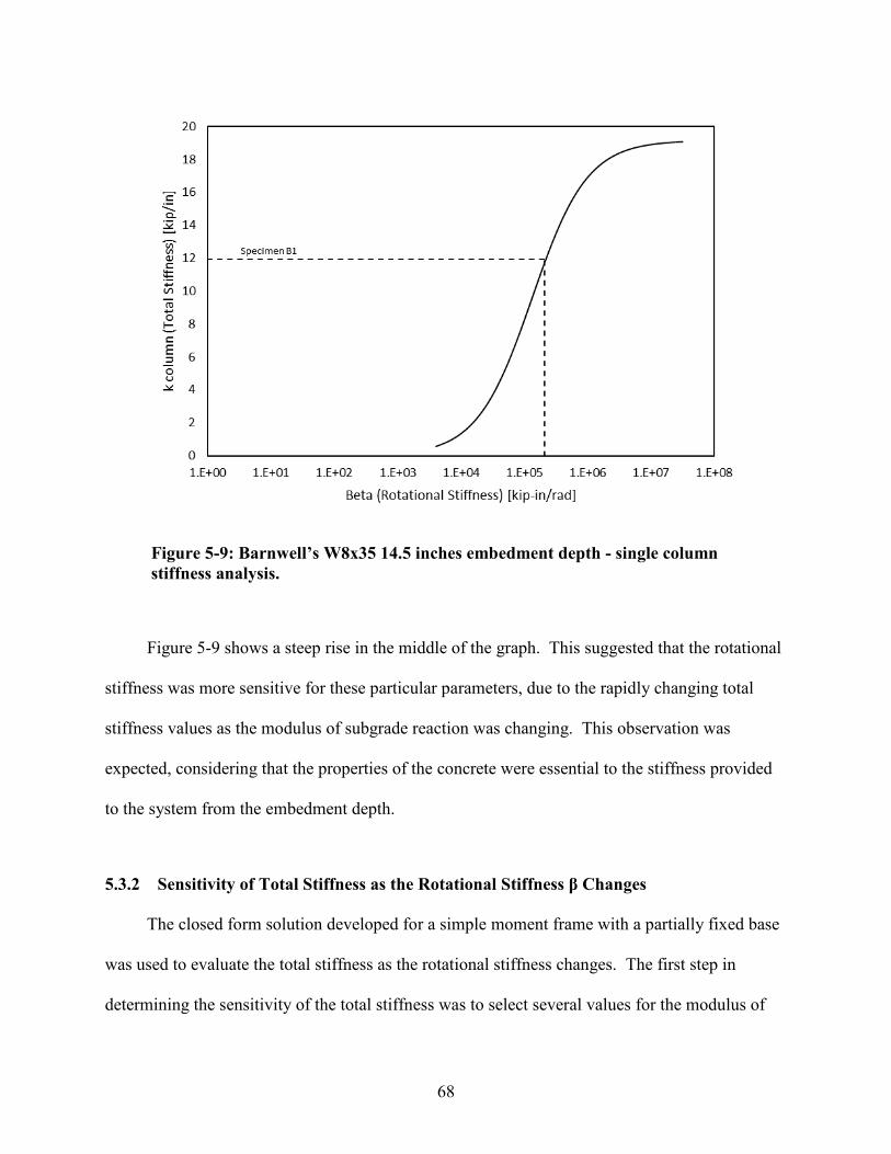
68
Figure 5-9 shows a steep rise in the middle of the graph. This suggested that the rotational
stiffness was more sensitive for these particular parameters, due to the rapidly changing total
stiffness values as the modulus of subgrade reaction was changing. This observation was
expected, considering that the properties of the concrete were essential to the stiffness provided
to the system from the embedment depth.
5.3.2 Sensitivity of Total Stiffness as the Rotational Stiffness β Changes
The closed form solution developed for a simple moment frame with a partially fixed base
was used to evaluate the total stiffness as the rotational stiffness changes. The first step in
determining the sensitivity of the total stiffness was to select several values for the modulus of
Figure 5-9: Barnwell’s W8x35 14.5 inches embedment depth - single column stiffness analysis.
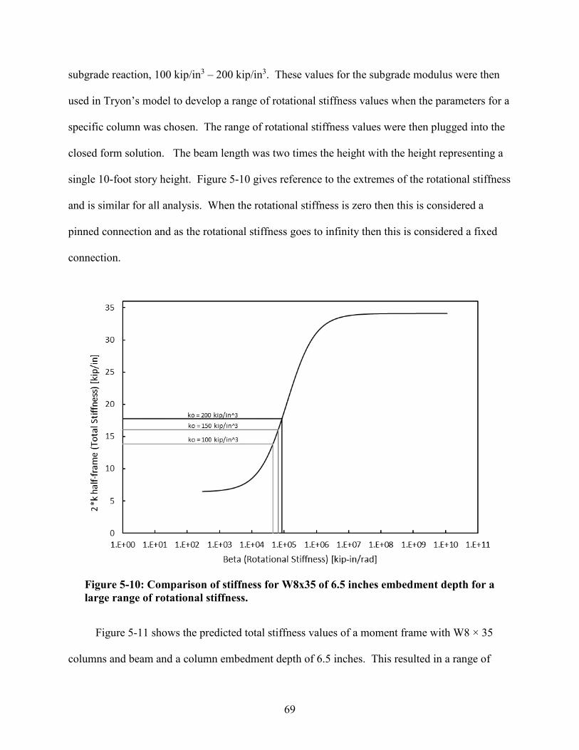
69
subgrade reaction, 100 kip/in3 – 200 kip/in3. These values for the subgrade modulus were then
used in Tryon’s model to develop a range of rotational stiffness values when the parameters for a
specific column was chosen. The range of rotational stiffness values were then plugged into the
closed form solution. The beam length was two times the height with the height representing a
single 10-foot story height. Figure 5-10 gives reference to the extremes of the rotational stiffness
and is similar for all analysis. When the rotational stiffness is zero then this is considered a
pinned connection and as the rotational stiffness goes to infinity then this is considered a fixed
connection.
Figure 5-10: Comparison of stiffness for W8x35 of 6.5 inches embedment depth for a large range of rotational stiffness.
Figure 5-11 shows the predicted total stiffness values of a moment frame with W8 × 35
columns and beam and a column embedment depth of 6.5 inches. This resulted in a range of
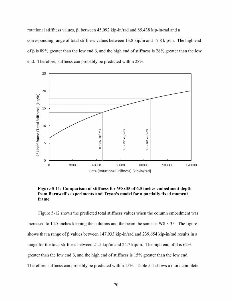
70
rotational stiffness values, β, between 45,092 kip-in/rad and 85,438 kip-in/rad and a
corresponding range of total stiffness values between 13.8 kip/in and 17.8 kip/in. The high end
of β is 89% greater than the low end β, and the high end of stiffness is 28% greater than the low
end. Therefore, stiffness can probably be predicted within 28%.
Figure 5-11: Comparison of stiffness for W8x35 of 6.5 inches embedment depth from Barnwell's experiments and Tryon's model for a partially fixed moment frame
Figure 5-12 shows the predicted total stiffness values when the column embedment was
increased to 14.5 inches keeping the columns and the beam the same as W8 × 35. The figure
shows that a range of β values between 147,933 kip-in/rad and 239,654 kip-in/rad results in a
range for the total stiffness between 21.5 kip/in and 24.7 kip/in. The high end of β is 62%
greater than the low end β, and the high end of stiffness is 15% greater than the low end.
Therefore, stiffness can probably be predicted within 15%. Table 5-1 shows a more complete
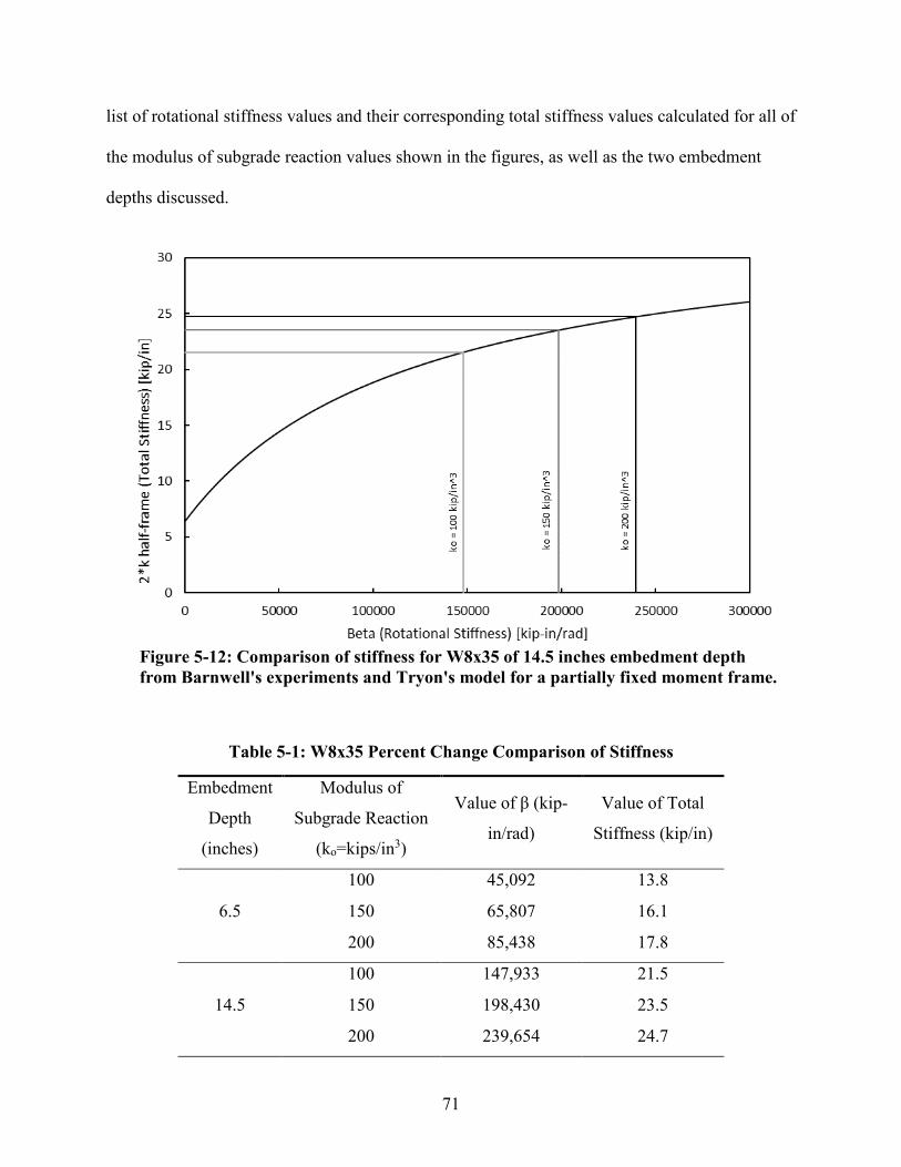
71
list of rotational stiffness values and their corresponding total stiffness values calculated for all of
the modulus of subgrade reaction values shown in the figures, as well as the two embedment
depths discussed.
Figure 5-12: Comparison of stiffness for W8x35 of 14.5 inches embedment depth from Barnwell's experiments and Tryon's model for a partially fixed moment frame.
Table 5-1: W8x35 Percent Change Comparison of Stiffness
Embedment
Depth
(inches)
Modulus of
Subgrade Reaction
(ko=kips/in3)
Value of β (kip-
in/rad)
Value of Total
Stiffness (kip/in)
6.5
100 45,092 13.8
150 65,807 16.1
200 85,438 17.8
14.5
100 147,933 21.5
150 198,430 23.5
200 239,654 24.7

72
Figure 5-13 shows the predicted stiffness values if a W10 × 77 was used for the columns
and beam; a column embedment depth of 7 inches was assumed. These assumptions resulted in
a range of rotational stiffness values between 300,809 kip-in/rad and 522,451 kip-in/rad and
resulted in a range of total stiffness values between 63.2 kip/in and 76.8 kip/in. The high end of
β is 74% greater than the low end β. The high end of stiffness is 21% greater than the low end.
Therefore, stiffness can probably be predicted within 21%.
Figure 5-13: Comparison of stiffness for W10x77 of 7 inches embedment depth from Hanks’ experiments and Tryon's model for a partially fixed moment frame.
Figure 5-14 shows the results for a moment frame with columns and beam with W10 × 77
shape, but the column embedment depth is increased to 15 inches. Figure 5-14, shows a range of

73
β values between 398,196 kip-in/rad and 626,350 kip-in/rad, which resulted with a total stiffness
range between 70.1 kip/in and 81.2 kip/in. The high end of β is 57% greater than the low end β.
The high end of stiffness is 16% greater than the low end. Therefore, stiffness can probably be
predicted within 16%. Table 5-2 shows a more complete list of rotational stiffness values and
total stiffness values calculated for all of the modulus of subgrade reaction values shown in the
figure, as well as the two embedment depths discussed.
Figure 5-14: Comparison of stiffness for W10x77 of 15 inches embedment depth from Hanks’ experiments and Tryon's model for a partially fixed moment frame.
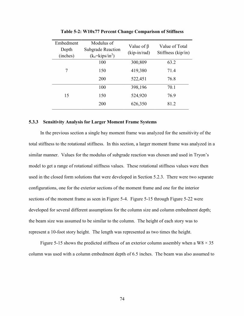
74
Table 5-2: W10x77 Percent Change Comparison of Stiffness
Embedment Depth
(inches)
Modulus of Subgrade Reaction
(ko=kips/in3)
Value of β (kip-in/rad)
Value of Total Stiffness (kip/in)
7
100 300,809 63.2
150 419,380 71.4
200 522,451 76.8
15
100 398,196 70.1
150 524,920 76.9
200 626,350 81.2
5.3.3 Sensitivity Analysis for Larger Moment Frame Systems
In the previous section a single bay moment frame was analyzed for the sensitivity of the
total stiffness to the rotational stiffness. In this section, a larger moment frame was analyzed in a
similar manner. Values for the modulus of subgrade reaction was chosen and used in Tryon’s
model to get a range of rotational stiffness values. These rotational stiffness values were then
used in the closed form solutions that were developed in Section 5.2.3. There were two separate
configurations, one for the exterior sections of the moment frame and one for the interior
sections of the moment frame as seen in Figure 5-4. Figure 5-15 through Figure 5-22 were
developed for several different assumptions for the column size and column embedment depth;
the beam size was assumed to be similar to the column. The height of each story was to
represent a 10-foot story height. The length was represented as two times the height.
Figure 5-15 shows the predicted stiffness of an exterior column assembly when a W8 × 35
column was used with a column embedment depth of 6.5 inches. The beam was also assumed to
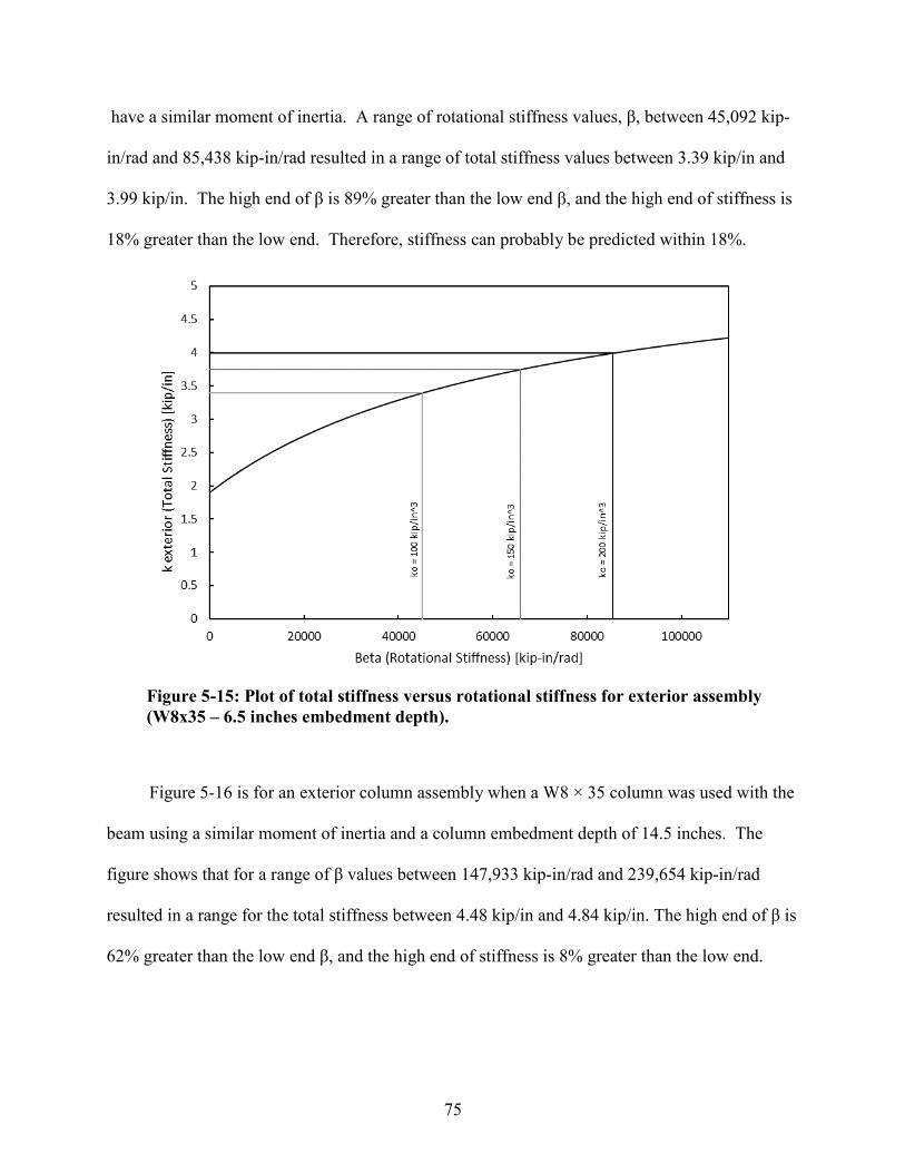
75
have a similar moment of inertia. A range of rotational stiffness values, β, between 45,092 kip-
in/rad and 85,438 kip-in/rad resulted in a range of total stiffness values between 3.39 kip/in and
3.99 kip/in. The high end of β is 89% greater than the low end β, and the high end of stiffness is
18% greater than the low end. Therefore, stiffness can probably be predicted within 18%.
Figure 5-15: Plot of total stiffness versus rotational stiffness for exterior assembly (W8x35 – 6.5 inches embedment depth).
Figure 5-16 is for an exterior column assembly when a W8 × 35 column was used with the
beam using a similar moment of inertia and a column embedment depth of 14.5 inches. The
figure shows that for a range of β values between 147,933 kip-in/rad and 239,654 kip-in/rad
resulted in a range for the total stiffness between 4.48 kip/in and 4.84 kip/in. The high end of β is
62% greater than the low end β, and the high end of stiffness is 8% greater than the low end.
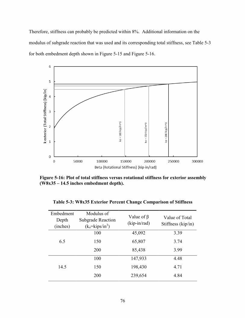
76
Therefore, stiffness can probably be predicted within 8%. Additional information on the
modulus of subgrade reaction that was used and its corresponding total stiffness, see Table 5-3
for both embedment depth shown in Figure 5-15 and Figure 5-16.
Figure 5-16: Plot of total stiffness versus rotational stiffness for exterior assembly (W8x35 – 14.5 inches embedment depth).
Table 5-3: W8x35 Exterior Percent Change Comparison of Stiffness
Embedment Depth
(inches)
Modulus of Subgrade Reaction
(ko=kips/in3)
Value of β (kip-in/rad)
Value of Total Stiffness (kip/in)
6.5
100 45,092 3.39
150 65,807 3.74
200 85,438 3.99
14.5
100 147,933 4.48
150 198,430 4.71
200 239,654 4.84
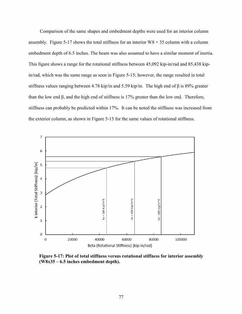
77
Comparison of the same shapes and embedment depths were used for an interior column
assembly. Figure 5-17 shows the total stiffness for an interior W8 × 35 column with a column
embedment depth of 6.5 inches. The beam was also assumed to have a similar moment of inertia.
This figure shows a range for the rotational stiffness between 45,092 kip-in/rad and 85,438 kip-
in/rad, which was the same range as seen in Figure 5-15; however, the range resulted in total
stiffness values ranging between 4.78 kip/in and 5.59 kip/in. The high end of β is 89% greater
than the low end β, and the high end of stiffness is 17% greater than the low end. Therefore,
stiffness can probably be predicted within 17%. It can be noted the stiffness was increased from
the exterior column, as shown in Figure 5-15 for the same values of rotational stiffness.
Figure 5-17: Plot of total stiffness versus rotational stiffness for interior assembly (W8x35 – 6.5 inches embedment depth).
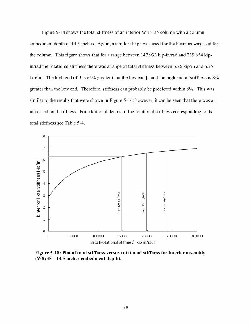
78
Figure 5-18 shows the total stiffness of an interior W8 × 35 column with a column
embedment depth of 14.5 inches. Again, a similar shape was used for the beam as was used for
the column. This figure shows that for a range between 147,933 kip-in/rad and 239,654 kip-
in/rad the rotational stiffness there was a range of total stiffness between 6.26 kip/in and 6.75
kip/in. The high end of β is 62% greater than the low end β, and the high end of stiffness is 8%
greater than the low end. Therefore, stiffness can probably be predicted within 8%. This was
similar to the results that were shown in Figure 5-16; however, it can be seen that there was an
increased total stiffness. For additional details of the rotational stiffness corresponding to its
total stiffness see Table 5-4.
Figure 5-18: Plot of total stiffness versus rotational stiffness for interior assembly (W8x35 – 14.5 inches embedment depth).

79
Table 5-4: W8x35 Interior Percent Change Comparison of Stiffness
Embedment Depth
(inches)
Modulus of Subgrade Reaction
(ko=kips/in3)
Value of β (kip-in/rad)
Value of Total Stiffness (kip/in)
6.5
100 45,092 4.78
150 65,807 5.26
200 85,438 5.59
14.5
100 147,933 6.26
150 198,430 6.57
200 239,653 6.75
A larger shape size was evaluated next for both the exterior column assembly as well as the
interior column assembly. Figure 5-19 shows the values for the total stiffness if a W10 × 77
exterior columns and the same shape for the beam was used. A column embedment depth of 7
inches was assumed. These assumptions resulted in a range of rotational stiffness values
between 300,809 kip-in/rad and 522,451 kip-in/rad and resulted in a range of total stiffness
values between 14.2 kip/in and 16.0 kip/in. The high end of β is 74% greater than the low end β,
and the high end of stiffness is 12% greater than the low end. Therefore, stiffness can probably
be predicted within 12%.
Figure 5-20 shows the values for the total stiffness if a W10 × 77 shape is used for the
exterior columns and a beam with similar moment of inertia as the column; however, with
15 inches of column embedment depth. This resulted in a range of rotational stiffness values
between 398,195 kip-in/rad and 626,350 kip-in/rad, which resulted in a total stiffness range
between 15.2 kip/in and 16.5 kip/in. The high end of β is 57% greater than the low end β, and the
high end of stiffness is 9% greater than the low end. Therefore, stiffness can probably be
predicted within 9%. For additional information on the results seen in Figure 5-19 and Figure
5-20 see Table 5-5.
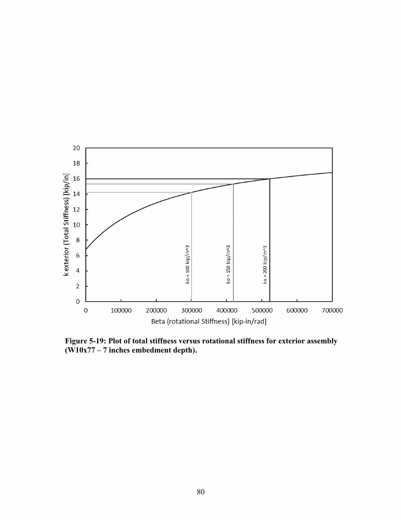
80
Figure 5-19: Plot of total stiffness versus rotational stiffness for exterior assembly (W10x77 – 7 inches embedment depth).
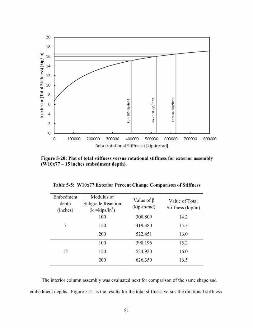
81
Figure 5-20: Plot of total stiffness versus rotational stiffness for exterior assembly (W10x77 – 15 inches embedment depth).
Table 5-5: W10x77 Exterior Percent Change Comparison of Stiffness
Embedment depth
(inches)
Modulus of Subgrade Reaction
(ko=kips/in3)
Value of β (kip-in/rad)
Value of Total Stiffness (kip/in)
7
100 300,809 14.2
150 419,380 15.3
200 522,451 16.0
15
100 398,196 15.2
150 524,920 16.0
200 626,350 16.5
The interior column assembly was evaluated next for comparison of the same shape and
embedment depths. Figure 5-21 is the results for the total stiffness versus the rotational stiffness

82
when a W10 × 77 column and beam was used for the interior assembly and a column embedment
depth of 7 inches. The figure shows a range for the rotational stiffness between 300,809 kip-
in/rad and 522,451 kip-in/rad, which was the same range as seen in Figure 5-19; however, this
range of β results in increased total stiffness values between 19.9 kip/in and 22.4 kip/in. The
high end of β is 74% greater than the low end β, and the high end of stiffness is 12% greater than
the low end. Therefore, stiffness can probably be predicted within 12%.
Figure 5-21: Plot of total stiffness versus rotational stiffness for interior assembly (W10x77 – 7 inches embedment depth).
Figure 5-22 is also for an interior column assembly using the W10 × 77 shape, a beam
shape of a similar moment of inertia, and 15 inches of column embedment depth. The figure
shows that the rotational stiffness ranges between 398,195 kip-in/rad and. 626,350 kip-in/rad.
This is the same range as seen in Figure 5-20; however, the range resulted in an increased total
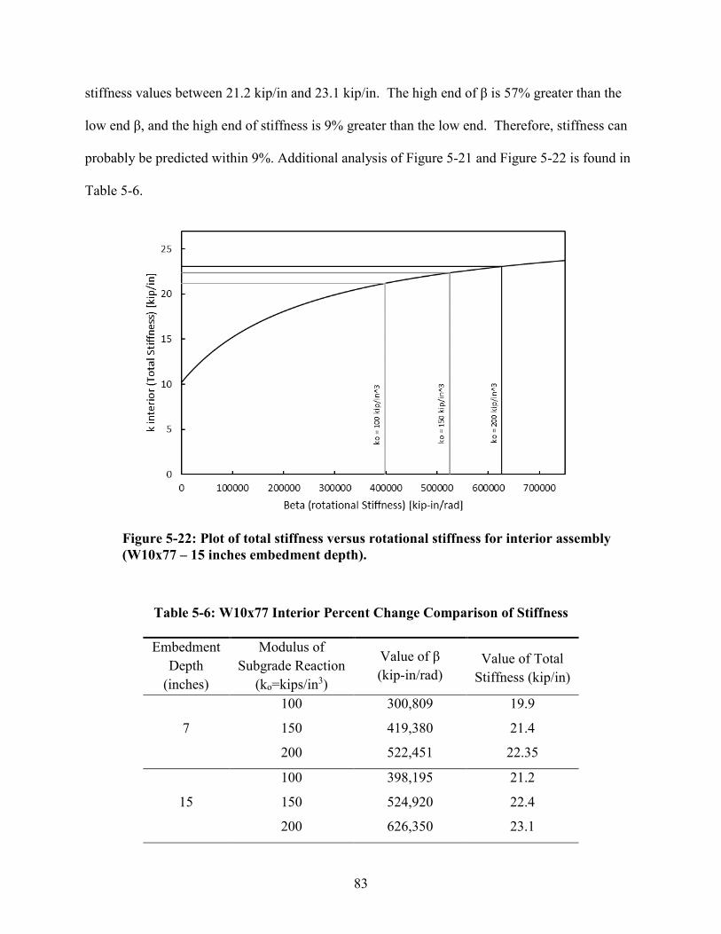
83
stiffness values between 21.2 kip/in and 23.1 kip/in. The high end of β is 57% greater than the
low end β, and the high end of stiffness is 9% greater than the low end. Therefore, stiffness can
probably be predicted within 9%. Additional analysis of Figure 5-21 and Figure 5-22 is found in
Table 5-6.
Figure 5-22: Plot of total stiffness versus rotational stiffness for interior assembly (W10x77 – 15 inches embedment depth).
Table 5-6: W10x77 Interior Percent Change Comparison of Stiffness
Embedment Depth
(inches)
Modulus of Subgrade Reaction
(ko=kips/in3)
Value of β (kip-in/rad)
Value of Total Stiffness (kip/in)
7
100 300,809 19.9
150 419,380 21.4
200 522,451 22.35
15
100 398,195 21.2
150 524,920 22.4
200 626,350 23.1

84
Summary
The total stiffness is very for values of β from around 1e+04 to 1e+06. However, the exact
values will vary as shown herein for the W10 and W8 columns. The effect of β remains semi-
regular for different shapes as well as for the different column configurations used during
investigation. The main difference was in the total stiffness per column. It was expected that the
moment frame with partial fixity at the base would have greater stiffness then a single partially
fixed column.
Better accuracy in predicting the rotational stiffness is obtained with better estimation of
the modulus of subgrade reaction; however, even if the rotational stiffness may only be predicted
to within a 100%, then the total stiffness of a partially fixed frame may be predicted only within
a 15% to 20% change. The percentage was reduced based on the type of configuration use.

85
6 CONCLUSIONS
This thesis outlined the work done to further the understanding of the rotational stiffness of
shallow embedded columns. This thesis evaluated the model created by Tryon with the data
collected from the physical test conducted by Barnwell and Hanks. The research completed for
this thesis resulted in creating an improved model.
The new model shows:
1. The modulus of subgrade reaction was a sensitive parameter for the model. However,
when the modulus of subgrade reaction is in the correct range for the column
connection then there is not a large change on the total stiffness.
2. The exposed length did not have a large effect on the model predicted results,
especially for small changes.
3. The modulus of concrete for the slab and the blockout had a large effect on the model
predicted results.
4. Flange effective width was not an influential parameter to the model. It appeared that
only one flange acted in resistance against the concrete blockout was a better
estimation.
5. The base plate thickness had a large effect on the predicted rotational stiffness, by
adjusting the effective column depth.

86
6. The model was not a good predictor for little to no embedment depth due to the lack of
specimen data.
7. Shallow embedded columns had a great deal more stiffness than a pinned system and
less stiffness than a fixed system.
8. Values for beta or the stiffness of the rotational spring were in the sensitive region;
however, a large change in the spring stiffness will result in a change of less than 20%
in the stiffness of the whole system.
This model was meant as an approximation and to give a good range for estimating
rotational stiffness values. However, it is important to use good judgement and check the limits
of your design, since, the number of anchor bolts, base plate thickness, embedment depth,
column and or beam size as well as the type of loads that the system is subjected to has a large
effect on the design. Different shapes other than the wide flange shape may not work with this
model.
Further research could be completed by adding in more data sets with more range in shape
sizes and embedment depths, so that more accurate curves can be developed. Additional tests
should be done for the weak orientation, since there were only two points in all the data
presented.
87
REFERENCES
Barnwell, N. V. (2015). Experimental Testing of Shallow Embedded Connections Between
Steel Columns and Concrete Footings. (Master of Science), Brigham Young University.
Cui, Y., Nagae, T., & Nakashima, M. (2009). Hysteretic behavior and strength capacity of
shallowly embedded steel column bases. Journal of structural engineering, 135(10), 1231-1238.
DeWolf, J. T., & Sarisley, E. F. (1980). Column base plates with axial loads and moments.
Journal of the Structural Division, 106(11), 2167-2184.
Fisher, J. M. and L. A. Kloiber (2006). Base Plate and Anchor Rod Design, 2nd Ed.
American Institute of Steel Construction.
Grilli, D. A., & Kanvinde, A. M. (2015). Embedded column base connections subjected to
flexure and axial load: Tests and strength models.
Grilli, D. A., & Kanvinde, A. M. (2017). Embedded column base connections subjected to
seismic loads: Strength model. Journal of Constructional Steel Research, 129, 240-249.
Hanks, K. N. (2016). Rotational Strength and Stiffness of Shallowly Embedded Base
Connections in Steel Moment Frames. (Master of Science), Brigham Young University.
Hetényi, M. (1971). Beams on elastic foundation: theory with applications in the fields of
civil and mechanical engineering: University of Michigan.
Kanvinde, A. M., & Deierlein, G. G. (2011). Recent research on column base connections.
Modern Steel Construction.
88
Kanvinde, A. M., Grilli, D. A., & Zareian, F. (2011). Rotational stiffness of exposed
column base connections: Experiments and analytical models. Journal of structural engineering,
138(5), 549-560.
Kanvinde, A. M., Jordan, S. J., & Cooke, R. J. (2013). Exposed column base plate
connections in moment frames-Simulations and behavioral insights. Journal of Constructional
Steel Research, 84, 82-93.
Rodas, P. T., Zareian, F., & Kanvinde, A.M. (2017). Rotational stiffness of Deeply
Embedded Column-Base Connections. Journal of structural engineering, 143(8): 04017064.
Sall, O. A., Fall, M., Berthaud, Y., & Ba, M. (2013). Influence of the Elastic Modulus of
the Soil and Concrete Foundation on the Displacements of a Mat Foundation. Open Journal of
Civil Engineering, 3(04), 228
Tryon, J. E. (2016). Simple Models for Estimating the Rotational Stiffness of Steel
Column-to-Footing Connections. (Master of Science), Brigham Young University.

89
APPENDIX A

Half Moment Frame With Nodes A, B, and C
Step 1: Construct indiviual member k matrix
k hat for member AB
khatab
E Ac
H
0
0
E Ac
H
0
0
0
12 E Ic
H3
6 E Ic
H2
0
12 E Ic
H3
6 E Ic
H2
0
6 E Ic
H2
4 E Ic
H
0
6 E Ic
H2
2 E Ic
H
E Ac
H
0
0
E Ac
H
0
0
0
12 E Ic
H3
6 E Ic
H2
0
12 E Ic
H3
6 E Ic
H2
0
6 E Ic
H2
2 E Ic
H
0
6 E Ic
H2
4 E Ic
H
=
T
0
1
0
0
0
0
1
0
0
0
0
0
0
0
1
0
0
0
0
0
0
0
1
0
0
0
0
1
0
0
0
0
0
0
0
1
= Transform so that the member is vertical
kab TT khatab T=
90
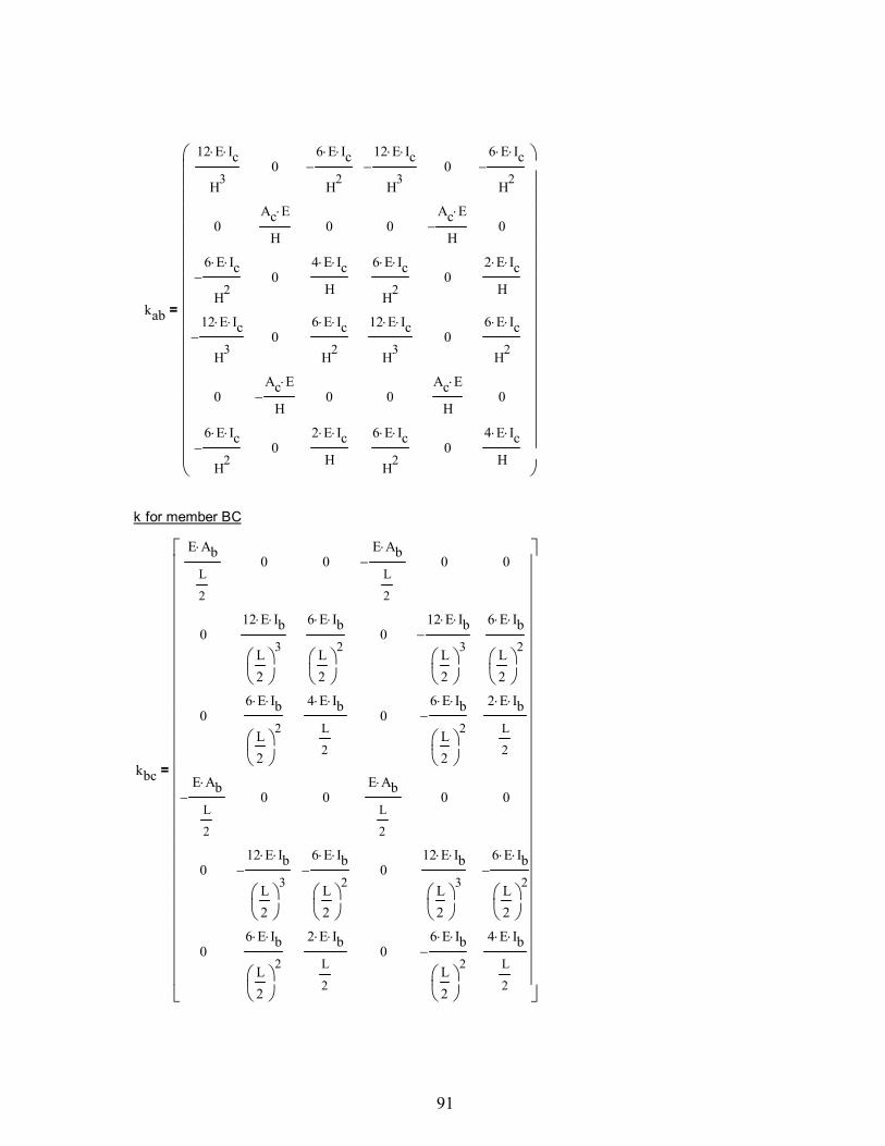
kab
12 E Ic
H3
0
6 E Ic
H2
12 E Ic
H3
0
6 E Ic
H2
0
Ac E
H
0
0
Ac E
H
0
6 E Ic
H2
0
4 E Ic
H
6 E Ic
H2
0
2 E Ic
H
12 E Ic
H3
0
6 E Ic
H2
12 E Ic
H3
0
6 E Ic
H2
0
Ac E
H
0
0
Ac E
H
0
6 E Ic
H2
0
2 E Ic
H
6 E Ic
H2
0
4 E Ic
H
=
k for member BC
kbc
E Ab
L
2
0
0
E Ab
L
2
0
0
0
12 E Ib
L2
3
6 E Ib
L2
2
0
12 E Ib
L2
3
6 E Ib
L2
2
0
6 E Ib
L2
2
4 E Ib
L
2
0
6 E Ib
L2
2
2 E Ib
L
2
E Ab
L
2
0
0
E Ab
L
2
0
0
0
12 E Ib
L2
3
6 E Ib
L2
2
0
12 E Ib
L2
3
6 E Ib
L2
2
0
6 E Ib
L2
2
2 E Ib
L
2
0
6 E Ib
L2
2
4 E Ib
L
2
=
91
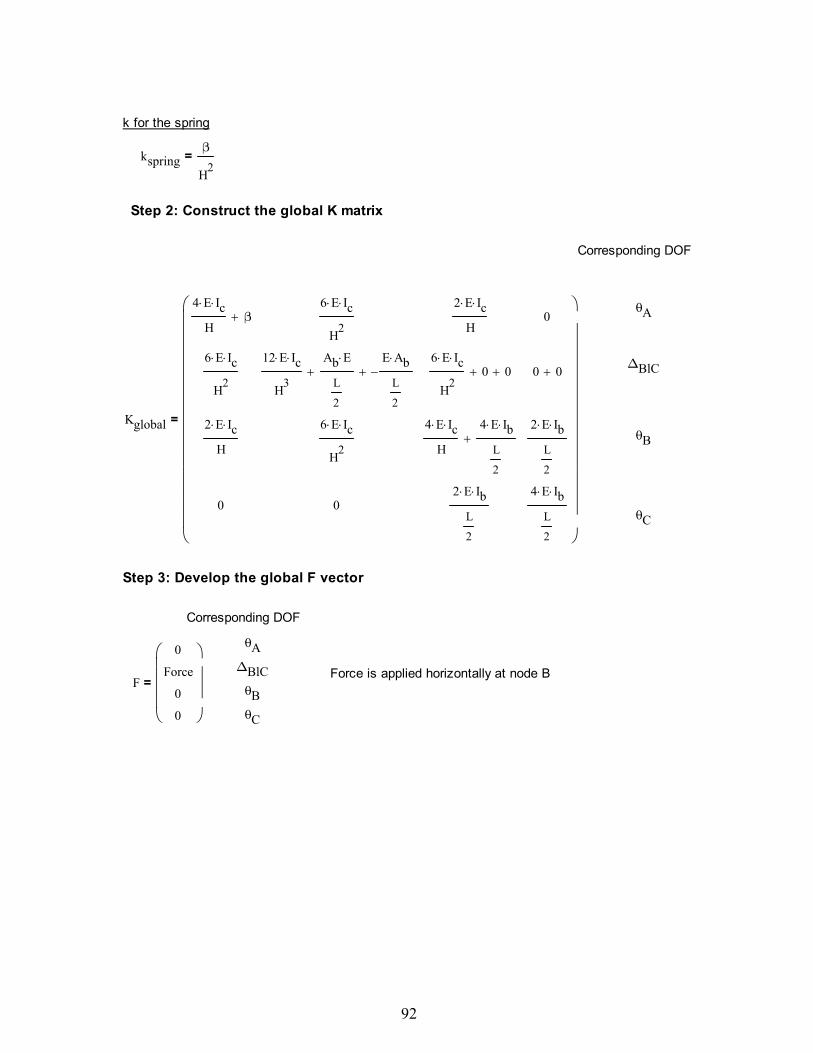
k for the spring
kspringβ
H2=
Step 2: Construct the global K matrix
Corresponding DOF
θA
ΔBlC
Kglobal
4 E Ic
Hβ
6 E Ic
H2
2 E Ic
H
0
6 E Ic
H2
12 E Ic
H3
Ab E
L
2
E Ab
L
2
6 E Ic
H2
0
2 E Ic
H
6 E Ic
H20 0
4 E Ic
H
4 E Ib
L
2
2 E Ib
L
2
0
0 0
2 E Ib
L
2
4 E Ib
L
2
=θB
θC
Step 3: Develop the global F vector
Corresponding DOF
θAΔBlC Force is applied horizontally at node B
F
0
Force
0
0
=θBθC
92

Step 4: Find all displacments and deformations
U Kglobal1 F= Corresponding DOF
θA
ΔBlC
U
Force 3 Ib H2 Ic L H
6 E Ib Ic 6 H Ib β Ic L β
Force 3 H4 Ib β 12 E H3
Ib Ic 2 H3 Ic L β 6 E H2
Ic2
L
36 Ib E2 Ic
2 6 L β E Ic
2 36 H Ib β E Ic
Force L β H2 2 E Ic L H
12 E2 Ib Ic 12 E H Ib β 2 E Ic L β
Force E Ic L H L β β H2 2 E Ic H
2 E Ic 2 H β 12 E2 Ib Ic 12 E H Ib β 2 E Ic L β
=θB
θC
Step 5: Determine the stiffness of the system at the base
Stiffness of the system is
KForceΔBlC
=
K36 Ib E2
Ic2
6 L β E Ic2
36 H Ib β E Ic
3 H4 Ib β 12 E H3
Ib Ic 2 H3 Ic L β 6 E H2
Ic2
L=
This is the stiffness for the half moment frame.
For the full moment frame use 2*K
93