Rotation-free triangular plate and shell elements - Cimne

INTERNATIONAL JOURNAL FOR NUMERICAL METHODS IN ENGINEERINGInt. J. Numer. Meth. Engng. 47, 557–603 (2000)

Rotation-free triangular plate and shell elements

Eugenio Onate∗ and Francisco Z�arateInternational Centre for Numerical Methods in Engineering; Universidad Polit�ecnica de Cataluna;

Gran Capit�an s=n; 08034 Barcelona; Spain

SUMMARY

The paper describes how the �nite element method and the �nite volume method can be successfully combinedto derive two new families of thin plate and shell triangles with translational degrees of freedom as the onlynodal variables. The simplest elements of the two families based on combining a linear interpolation ofdisplacements with cell centred and cell vertex �nite volume schemes are presented in detail. Examples ofthe good performance of the new rotation-free plate and shell triangles are given. Copyright ? 2000 JohnWiley & Sons, Ltd.

KEY WORDS: rotation-free; thin plate and shell triangles; �nite elements; �nite volumes

INTRODUCTION

The need for e�cient plate and shell elements is essential for solving large-scale industrial prob-lems such as the analysis of shell structures in civil, mechanical, naval and airspace engineering,the study of vehicle dynamics and crash-worthiness situations and the design of sheet metal form-ing processes among others. Despite recent advances in the �eld [1–3], the derivation of simpletriangles capable of accurately representing the deformation of a plate or a shell structure undercomplex loading conditions is still nowadays a challenging topic of intensive research.The development of plate (and shell) �nite elements was initially based on the so called thin

plate theory following Kirchho�’s main assumption of preserving orthogonality of the normals tothe mid-plane [1; 4]. Indeed, most plates and shells can be classed as ‘thin’ structures and there-fore Kirchho�’s theory can reproduce the essential features of the deformation in many practicalcases. The well known problems to derive conforming C1 continuous thin plate and shell elementsmotivated a number of authors to explore the possibilities of Reissner–Mindlin theory. This theoryrelaxes the normal orthogonality condition, thereby introducing the e�ect of shear deformationwhich can be of practical importance in thick situations, such as the analysis of some bridge slabsand, more important, it requires only C0 continuity for the de ection and rotation �elds. Unfortu-nately Reissner–Mindlin plate and shell elements su�er from the so called ‘shear locking’ de�ectwhich pollutes the numerical solution in the thin limit. This de�ciency has jeopardized the fullsuccess of Reissner–Mindlin plate=shell elements for practical engineering analysis, an exception

∗ Correspondence to: Eugenio Onate, International Centre for Numerical methods in Engineering, Universidad Polit�ecnicade Cataluna, edi�cio C1, Campus Norte UPC, Gran Capit�an s=n, 08034 Barcelona, Spain. E-mail: [email protected]

CCC 0029-5981/2000/030557–47$17.50 Received 10 March 1999Copyright ? 2000 John Wiley & Sons, Ltd.

558 E. ONATE AND F. Z �ARATE

perhaps being the four node quadrilateral based on an assumed shear strain formulation developedby Dvorkin and Bathe [5]. Thus, despite considerable e�orts [6–23] there are not yet well estab-lished simple triangles which are currently used for solving large-scale industrial plate and shellproblems.This paper presents a general approach to derive very simple plate and shell triangular elements

incorporating the displacements as the only nodal variables. The elements are based on Kirchho�’sthin plate theory and as such can be viewed as a return to the origins of plate and shell �niteelements. Indeed for the applications in mind such as the analysis of standard thin plate and shellanalysis, vehicle crash-worthiness and sheet stamping processes, Kirchho�’s theory su�ces forpractical purposes.The idea of using the de ection as the only nodal variable for plate bending analysis is not

new and many �nite di�erence (FD) procedures are based on this approach [24]. The obviousdi�culties of FD techniques are the treatment of boundary conditions and the problems for dealingwith non-orthogonal or unstructured grids.Several authors have tried to derive plate and shell �nite elements with displacements as the

nodal variables. So far the methods limit their applicability to triangular shapes only. The �rstattempt was probably due to Nay and Utku [25] who derived a rotation free thin plate triangle usinga least-square quadratic approximation to describe the de ection �eld within the patch surroundinga node in terms of the de ections of the patch nodes. The sti�ness matrix of the resulting threenode plate triangle were computed by the standard minimum potential energy approach. A fewyears later Barnes [26] proposed a method for deriving a three node plate triangle with the nodalde ections as the only degrees of freedom (d.o.f.) based on the computation of the curvaturesin terms of the normal rotations at the mid-side points determined from the nodal de ections ofadjacent elements. This method was exploited by Hampshire et al. [27] assuming that the elementsare hinged together at their common boundaries, the bending sti�ness being represented by torsionalsprings resisting the rotations about the hinge lines. Phaal and Calladine [28; 29] proposed asimilar class of rotation-free triangles for plate and shell analysis. Yang et al. [30] derived afamily of triangular elements of this type for sheet stamping analysis based on so called bendingenergy augmented membrane approach which basically reproduces the hinge bending sti�nessprocedure of Hampshire et al. [27]. Brunet and Sabourin [31] proposed a di�erent approach tocompute the constant curvature �eld within each triangle in terms of the six node displacementsof a macro-element. The triangle was successfully applied to non-linear shell analysis using anexplicit dynamic approach. Rio et al. [32] have used the concept of side hinge bending sti�ness toderive a thin shell triangle of ‘translational’ kind for explicit dynamic analysis of sheet stampingproblems.In 1993 Onate and Cervera [33] proposed a general procedure based on �nite volume concepts

[34–36] for deriving thin plate elements of triangular and quadrilateral shapes with the nodal de- ection as the only degree of freedom and presented a competitive and simple three d.o.f. triangle.In this work the ideas presented in [33] are extended to derive new rotation-free plate and shellelements. The basic ingredients of the derivation are a mixed Hu–Washizu formulation, a standarddiscretization of the plate surface into three node triangles, a linear �nite element (FE) approxi-mation of the displacement �eld within each triangle and a �nite volume (FV) type approach forcomputing the curvature and bending moment �elds within appropriate non-overlapping controldomains. Basically two modalities of control domains will be considered here, leading each toa di�erent plate triangle: the so called ‘cell centred’ patch formed by each individual triangle,leading to the BPT plate triangle and the BST shell triangle, and the ‘cell vertex’ domain formed

Copyright ? 2000 John Wiley & Sons, Ltd. Int. J. Numer. Meth. Engng. 47, 557–603 (2000)

ROTATION-FREE TRIANGULAR PLATE AND SHELL ELEMENTS 559

Figure 1. Sign convention for the de ection and the rotations in a plate

by the non-overlapping nodal regions, leading to the BPN and BSN plate and shell triangles,respectively.The layout of the paper is the following. In the next section the basic concepts of Kirchho�’s

plate theory are given and the set of governing equations emerging from the standard Hu–Washizuformulation are described. Next, details of the combined �nite element=�nite volume approach usedin the formulation of the rotation free BPT and BPN plate triangles are described. An extensionof the BPT element based on a linear least-square interpolation of the de ection gradients overan element patch is also presented. The relevant matrices and vectors for each case are given inexplicit form. The formulation of the rotation-free BST and BSN shell triangles is then describedas an extension of the parent thin plate formulation. Examples of the e�ciency of the new trianglesfor a wide range of plate and shell problems are �nally presented.

BASIC THEORY

Let us consider the plate of Figure 1. We will assume Kirchho�’s thin plate conditions to hold, i.e.

�x = @w=@x and �y = @w=@y (1)

The curvatures �eld and the moment–curvature relationship can be expressed in the usual manneras

Z=Lw; m=DZ (2)

with

Z= [�x; �y; �xy]T; m= [mx; my; mxy]T

L=[− @2

@x2;− @2

@y2;−2 @2

@x@y

]T; D=

Et3

12(1− �2)

1 � 0� 1 0

0 01− �2

(3)

where E and � are the Young’s modulus and the Poisson’s ratio, respectively, and t is the platethickness.



The set of governing equations will be expressed in integral form starting from the standardHu–Washizu functional [1]

�=12

∫∫AZTDZ dA−

∫∫A[Lw − Z]Tm dA−

∫∫Aqw dA (4)

where q is the distributed loading and A is the area of the plate. Variation of � with respect toZ; m and w leads to the following three equations:

Constitutive equation ∫∫A�ZT[DZ −m] dA=0 (5a)

Curvature-de ection equation ∫∫A�mT[Lw − Z] dA=0 (5b)

Equilibrium equation ∫∫A[L�w]Tm dA−

∫∫A�wq dA=0 (5c)

Equations (5a)–(5c) represent the global satisfaction over the plate of the constitutive, kinematicand equilibrium equations, respectively. Equations (5) are the basis of the FE=FV discretizationto be presented next.

FINITE ELEMENT=FINITE VOLUME DISCRETIZATION

Let us consider an arbitrary discretization of the plate into standard three node triangles. The curva-ture and the bending moments are described by constant �elds within appropriate non-overlappingcontrol domains (also termed ‘control volumes’ in the FV literature [34–36]) covering the wholeplate as

m= I3mp; �m= I3�mp (6a)

Z= I3Zp; �Z= I3�Zp (6b)

where I3 is the 3× 3 unit matrix and (·)p denotes constant values for the pth control domain.Two modalities of control domains are considered: (a) that formed by a single triangular ele-

ment (Figure 2(a)) and (b) the control domain formed by one-third of the areas of the elementssurrounding a node (Figure 2(b)). The two options are termed in the FV literature ‘cell centred’and ‘cell vertex’ schemes, respectively.Note that in the cell centred scheme each control domain coincides with a standard three node

�nite element triangle. Alternatively in the cell vertex scheme a control domain is contributed bydi�erent elements, as shown in Figure 2(b).It is also useful to de�ne the term ‘patch of elements’ associated to a control domain. In the cell

centred scheme (Figure 2(a)) this patch is always formed by four elements (except in elementssharing a boundary segment), whereas in the cell vertex scheme the number of elements in thepatch is variable (Figure 2(b)).



Remark 1. The name ‘Cell Centred’ (CC) indicates that the chosen variables (i.e. the curvaturesand bending moments) are ‘sampled’ at the center of the cells discretizing the analysis domain(i.e. the three node triangles). Similarly a ‘Cell Vertex’ (CV) scheme denotes that the variablesare sampled at the corners (i.e. the nodes) of the discretizing grid. This terminology has su�eredsome controversial interpretations in the past (for instance in [33; 34] a di�erent criterion waschosen). The meaning given here to the CC and CV schemes corresponds to above de�nition.The constant curvature and bending moment �elds within each control domain are expressed

next in terms of the nodal de ections associated to the corresponding element patch.The area integrals in equations (5) can be written as sum of contributions over the di�erent

control domains taking into account equations (6) as

Constitutive equation

∑p

∫∫Ap�ZTp [DZp −mp] dA=0 (7)

where Ap is the area of the pth control domain.Recalling that the virtual curvatures are arbitrary, gives

mp=DpZp (8a)

Dp=1Ap

∫∫ApD dA (8b)

where Dp is the average constitutive matrix over a control domain. Equation (8a) de�nes theconstant bending moment �eld over the control domain in terms of the corresponding constantcurvatures.

Curvature-de ection equation

∑p

∫∫Ap�mTp [Lw − Zp] dA=0 (9)

Taking into account that the virtual bending moments are arbitrary, gives

Zp=1Ap

∫∫ApLw dA (10)

A simple integration by parts of the r.h.s. of equation (10) leads to

Zp=1Ap

∫�pT∇w d� (11)

where

T=

[−nx 0 −ny0 −ny −nx

]T; ∇=

@@x@@y

(12)



Figure 2. (a) Cell centred and (b) cell vertex �nite volume schemes. BPT and BPN triangles

and n= [nx; ny]T is the outward unit normal to the boundary �p surrounding the control domain(Figure 2).Equation (11) de�nes the curvatures for each control volume in terms of the de ection gradients

along its boundaries. The transformation of the area integral of equation (10) into the line integralof equation (11) is typical of �nite volume methods [33–36].

Remark 2. The computation of the line integral in equation (11) poses a di�culty for caseswhere the de ection gradient is discontinuous at the control volume boundaries and some smooth-ing procedure is then required. This issue is discussed in more detail in a later section.

Equilibrium equationEquation (5c) can be expressed as

∑p

∫∫Ap[L�w]Tmp dA−

∫∫A�wq dA=0 (13)

Integrating by parts the �rst integral in equation (13) and recalling that the bending momentsare constant within each control domain, gives

∑p

(∫�p[T∇�w]T d�

)mp −

∫∫A�wq dA=0 (14)

Substituting equations (8a) and (11) into equation (14) �nally gives

∑p

(∫�p[T∇�w]T d�

)1ApDp∫�pT∇w d�−

∫∫A�wq dA=0 (15)

Equation (15) is the basis for deriving the �nal set of algebraic equations, after appropriatediscretization of the de ection �eld as described next.



Derivation of the discretized equations

The �nal step is to discretize the de ection �eld. The simplest option is to interpolate linearlythe de ection within each triangular element in terms of the nodal values in the standard �niteelement manner [1] as

w=3∑i=1Niwi=N(e)w(e) (16)

with N(e) = [N1; N2; N3] and w(e) = [w1; w2; w3]T. In equation (16) wi denotes the nodal de ectionvalues and Ni are the standard linear shape functions of the three node triangle [1]. Substitutingequations (16) into (11) gives

Zp=1Ap

∫�pT∇N(e)w(e) =Bpwp (17)

where vector wp lists the de ections of the nodes linked to the pth control domain and Bp isthe curvature matrix relating the constant curvature �eld within a control domain and the nodalde ections associated to the control domain. The computation of matrix Bp is di�erent for cellvertex and cell centred schemes and the details are given in next sections.Substituting equations (16) into (15) gives the �nal system of algebraic equations as

Kw= f (18)

where vector w contains the nodal de ections of all mesh nodes. The global sti�ness matrix K canbe obtained by assembling the sti�ness contributions from the di�erent control domains given by

Kp= [Bp]TDpBpAp (19)

The components of the nodal force vector f in equation (18) are obtained as in standard C0linear �nite element triangles [1], i.e.

Point loading

fi=pi (20)

where pi is the point load acting on the ith node

Distributed loading

f(e)i =∫∫

A(e)Niq(x) dA (21)

The global nodal force component fi is obtained by assembling the element contributions f(e)i

in the standard �nite element manner. For a constant distributed load q this gives

fi=∑e

qA(e)

3(22)

where the sum extends to all triangular elements sharing the ith node and A(e) is the area ofelement e.



Box I. Matrix Bp for the 3 d.o.f. basic plate triangle (BPT)

Bp=1Ap

yij �b(b)i + yki �b

(d)i yij �b

(b)j + yjk �b

(c)j yjk �b

(c)k + yki �b

(d)k

−xij �c (b)i − xki �c (d)i −xij �c (b)j − xjk �c (c)j −xjk �c (c)k − xki �c (d)k[yij �c

(b)i − xij �b(b)i

[yij �c

(b)j − xjk �b(b)j

[yjk �c

(c)k − xjk �b(c)k

+yki �c(d)i − xki �b (d)i

]+yjk �c

(c)j − xjk �b(c)j

]+yki �c

(d)k − xki �b (d)k

]yij �b

(b)l yjk �b(c)m yki �b(d)n

−xij �c (b)l −xjk �c (c)m −xki �c (d)nyij �c

(b)l − xij �b(b)l yjk �c(c)m − xjk �b(c)m yki �c (d)n − xki �c (d)n

�b(e)i =b(e)i2A(e)p

; �c (e)i =c (e)i2A(e)p

; b(e)i =y(e)j − y(e)k ci= x(e)k − x(e)j ; etc:; Ap=A(p)

CELL CENTERED PATCH BPT ELEMENT

The evaluation of the constant curvature �eld in equation (11) requires the computation of thede ection gradient along the control domain boundaries. This poses a di�culty in cell cen-tred con�gurations where each control domain coincides with an individual element. Here if thede ection is linearly interpolated within each triangle, then the term ∇w is discontinuous at theelement sides. A simple method to overcome this problem proposed by Onate and Cervera [33]is to compute the de ection gradients at the triangle sides as the average value of the gradientscontributed by the two elements sharing the side. The constant curvature �eld for each controldomain can be expressed in this case as

Zp=1Ap

3∑j=1

l(p)j

2T(p)j

[∇N(p)w(p) +∇N(k)w(k)] =Bpwp (23a)

with

wp= [wi; wj; wk ; wl; wm; wn]T (23b)

In equation (23a) the sum extends over the three sides of element p coinciding with the pthcontrol domain, T(p)j is the transformation matrix of equation (12) for side j; l(p)j are the lengthsof the element sides, Ap=A(p) is the area of the fth triangle and superindex k refers to each ofthe elements adjacent to element p (k = a; b; c for j=1; 2; 3. See Figure 2(a)).The computation of the curvature matrix is simple noting that the gradients of the shape functions

are constant within each element. The explicit form of matrix Bp is given in Box I.Note that Bp in this case is a 3× 6 matrix relating the de ections of the six nodes of the four

element patch contributing to the control domain. Consequently the sti�ness matrix Kp is a 6× 6matrix.The resulting plate element is identical to that derived by Onate and Cervera [33] and it is

termed BPT (for Basic Plate Triangle). The element can be viewed as a standard �nite element



Figure 3. Basic plate triangle (BPT) next to a boundary line

plate triangle with one degree of freedom per node and a wider bandwidth, as each element islinked to its neighbours through equation (23a).

Boundary conditions for the BPT element

The implementation of the boundary conditions is straightforward and the main di�erence withstandard �nite elements is that the conditions on the prescribed rotations must be imposed whenthe curvature matrices Bp are being built. The di�erent situations are considered next.A BPT element with a side along a boundary edge has one of the elements contributing to the

patch missing. This is simply taken into account by ignoring this contribution when performingthe average of the de ection gradient in equation (23a). Thus, if side 1 corresponding to nodes ijlies on the boundary (Figure 3), the curvature �eld for the control domain is obtained by

Zp=lijApT (p)1 ∇N(p)w(p) + 1

Ap

3∑j=2

l(p)j

2T (p)j [∇N(p)w(p) +∇N(k)w(k)] =Bpwp (24)

Additional conditions must be imposed in the case of boundary edges where the rotations and=orthe de ections are constrained as explained next.

Clamped edge (w=∇w=0)The conditions on the rotations are simply imposed by disregarding the contributions from the

clamped edges when computing the sum along the element sides in equation (23a). For instance,if side ij is clamped this simply implies making zero the �rst term in the r.h.s. of equation (24).The condition w=0 on the nodes laying on clamped edges is prescribed at the equation solution

level in the standard manner.

Symmetry edge (@w=@x=0 or @w=@y=0)The condition of zero rotation is imposed by neglecting the contribution from the prescribed

rotation term (@w=@x or @w=@y) at the symmetry edge when computing equation (23a).

Simply supported edge (w= @w=@s=0)The condition @w=@s=0, where s is the boundary direction, is simply imposed by prescribing

w=0 in the boundary nodes at the global equation solution level in the standard fashion. Thee�ect of the ‘missing’ contributing element at the boundary edge is accounted for by skipping theaveraging of the de ection gradient for that edge as described above.



BPT1 ELEMENT

An interesting alternative to the BPT element can be derived by de�ning a linear de ection gradient�eld over the four element patch. The simplest procedure is to use a least-square approximation ofthe de ection gradients computed at the centroids of the four elements contributing to the controldomain (Figure 2(a)). This avoids the averaging procedure of equation (23a) as the de ectiongradient is now continuous over the control volume. The basic ingredients of the element, termedBPT1, are given next.The de ection gradient is de�ned linearly over the four elements patch as

∇w={a1a2

}+{b1b2

}x +

{c1c2

}y= a + bx + cy (25)

The a; b and c parameters are obtained by minimizing the following quadratic form:

Jp=4∑i=1[(∇w)i − (a + bxi + cyi)]2 (26)

with respect to the parameters ai; bi; ci:In equation (26) (∇w)i are the de ection gradients computed at the centroid (xi; yi) of each of

the four elements linked to the pth control domain. It can be easily shown that

(∇w)i= 12A(i)

3∑j=1

{�(i)j�(i)j

}wj (27)

with �(i)j =y(i)k − y(i)l ; �(i)j = x(i)l − x(i)k for an element with nodes j; k; l [1].

In equation (27) A(i) is the area of the ith element and x(i)j ; y(i)j ; j=1; 2; 3; are the coordinates

of the element nodes.Minimization of Jp gives

[a1; b1; c1]T =C−1GSxwp (28a)

[a2; b2; c2]T =C−1GSywp (28b)

where wp is given by equation (23b) and the form of the matrices C;G;Sx and Sy is shown inBox II.Equation (25) can be used to compute the curvature vector for each control domain using

equation (11) as

Zp=1Ap

∫�pT[a + bx + cy]d�=

1Ap

3∑j=1T (p)j [a + bxj + cyj]lj =Bpwp (29)

where the sum extends to the three edges of the control domain, xj; yj are the coordinates of themid-point of the jth edge and lj is the edge length. The expression of Bp in this case can be easilydeduced substituting equations (28) into equation (29).The treatment of the boundary conditions follows the same procedure as for the BST element.

Naturally in a control volume sharing a boundary edge, the linear interpolation of the de ection�eld is then exact as only three elements are involved in the approximation. Also, the contributionof edges where the rotation is prescribed to a zero value is neglected in the sum of equation (29).



Box II. Matrices involved in the derivation of the BPT1 element

C=4∑i=1

1 xi yixi x2i xiyiyi xiyi y2i

; G=

1 1 1 1

x1 x2 x3 x4y1 y2 y3 y4

Sx =

�� (1)1 �� (1)2 �� (1)3 0 0 0

�� (2)3 �� (2)2 0 �� (2)1 0 0

0 �� (3)3 �� (3)2 0 �� (3)1 0

�� (4)2 0 �� (4)3 0 0 �� (4)1

Sy =

��(1)1

��(1)2

��(1)3 0 0 0

��(2)3

��(2)2 0 ��

(2)1 0 0

0 ��(3)3

��(3)2 0 ��

(3)1 0

��(4)2 0 ��

(4)3 0 0 ��

(4)1

with �� (i)1 =1A(i)

(y(i)3 − y(i)2 ); ��(i)1 =

1A(i)

(x(i)2 − x(i)3 ); etc:

Remark 3. The curvature matrix for the BPT1 element can be readily derived by using theoriginal form of equation (10) as the second derivatives of the de ection �eld can be directlycomputed from equation (25). The result is obviously the same in both cases.

Remark 4. The interpolation of the de ection �eld can be enhanced using weighted least-squareinterpolation techniques [37].



Figure 4. BPN element. Example of a typical control domain and numbering of nodes

Remark 5. The performance of the BPT and BPT1 elements is identical for regular structuredmeshes as the sti�ness matrices are the same in both cases. In non-structured meshes the perfor-mance of the BPT1 element is slightly superior as it will be shown in the examples.

CELL VERTEX PATCH. BPN ELEMENT

As mentioned earlier, a di�erent class of rotation-free plate triangles can be derived starting fromthe so called cell vertex �nite volume scheme (Figure 2(b)). The advantage of the cell vertexscheme is that the de ection gradient is now continuous along the control domain boundaries.This allows to compute directly the constant curvature vector over the control domain as

Zi=1Ai

∫�iT∇Niwi d�=Biwi (30)

where Ni contains contributions from the shape functions from all the elements participating inthe ith nodal control domain. Equation (30) can be rewritten in a simpler form taking into accountthat the de ection gradients are constant within each element, as

Zi=1Ai

∑j

lj2Tj∇N(j)w(j) =Biwi (31)

where the sum extends over the ni elements contributing to the ith control domain (for instanceni=5 in the patch of Figure 4), lj is the external side of element j; Tj is the transformation matrixof equation (12) linked to the side lj, superindex j refers to element values and Ai= 1

3

∑nik=1 A

(k)

where A(k) is the area of element k.The computation of the curvature matrix Bi is not so straightforward in this case as its size

depends on the variable number of nodes over the element patch contributing to a nodal controldomain (see Figure 4).Typically

1 2 : : : pnBi3×n

= [Bi Ba; : : : ; Br] (32)



Box III. Example of derivation of the curvature matrix for theBPN control domain of Figure 4

Bi= [Bi ;B j;Bk ;Bl;Bm;Bn]

Bi=12Ai

[laTaG

(a)1 + lbTbG

(b)1 + lcTcG

(c)1 + ldTdG

(d)1 + leTeG

(e)1

]

B j =12Ai

[laTaG

(a)2 + leTeG

(e)3

]

Bk =12Ai

[laTaG

(a)3 + lbTbG

(b)2

]

Bl=12Ai

[lbTbG

(b)3 + lcTcG

(c)2

]

Bm=12Ai

[lcTcG

(c)3 + ldTdG

(d)2

]

Bn=12Ai

[ldTdG

(d)3 + leTeG

(e)2

]

G(k)i =∇N (k)i =1

2A(k)

{bici

}(k); b(k)i =y(k)j − y(k)k ; c(k)i = xk − x(k)j

where pn is the number of nodes in the patch (i.e. pn=6 in the patch of Figure 4) and superindexesi; a; : : : ; r refer to global node numbers. An explicit expression of the nodal curvature matrix Bi

can be found as

Bi3×1

=12Ai

∑klkTk∇N (k)j (33)

where the sum extends now over the elements sharing node i within the patch and j is the localnumber of node i within element k. An example of matrix Bi for a typical control domain isshown in Box III.It is important to note that Bi is in this case the global curvature matrix for the central ith node.

Thus, the product BTi DiBiAi provides the ith row of the global sti�ness matrix. This simpli�es theassembly and solution process as the global sti�ness equations for a node can be elliminated oncethey are computed.Indeed the standard ‘element’ sti�ness matrix can be found by adding the contribution of the

three internal domains participating into each triangular element as shown in Figure 5. This,however, has been found not useful for practical purposes and the direct assembly of the controldomain contributions as explained above is recommended.



Figure 5. Contribution of control domains to a BPN tri-angular element in the cell vertex scheme

Figure 6. BPN element. Control domain sharing a boundaryline. Integration path for computation of curvature matrix

This plate element is termed BPN (for Basic Plate Nodal patch). Note that the concept of‘element’ here is generalized as the BPN element combines a standard �nite element interpolationwith non-standard integration domains.

Boundary conditions for the BPN element

The method for imposing the boundary conditions in the BPN element follows the lines pre-viously explained for the BPT element. The procedure is now simpler as the de ection gradientnow is continuous along the control domain boundary which intersects the central node in thiscase (Figure 6). As usual, the conditions on nodal de ections are imposed at the global solutionlevel while the prescribed rotations must be treated when building the curvature matrix.

Clamped and symmetry edgesZero rotation conditions at clamped and symmetry edges are simply imposed by elliminating

the contributions from these rotation terms in the sum of equation (31).

Simple supported edgesThe condition @w=@s=0 along an edge direction is simple accounted for by prescribing the

de ections of the edge nodes to a zero value at the global solution level.

Free edgesNo special treatment for the rotations is required at free edges. Advantage can be taken from

the mixed formulation in this case by prescribing the edge bending moments Mn and Msn to azero value. This can be simply done by eliminating the contributions from these moments at freeedge patches by making zero the appropriate rows in the constitutive matrix D. Indeed if thefree edge is not parallel to one of the cartesian axes a transformation of the constitutive equationto edge axes is then necessary.This procedure can also be applied to impose the condition Mn=0 at simply supported edges.



Figure 7. BST element. Control domain and four elements patch

BASIC SHELL TRIANGLE (BST)

The BPT element of previous section can be combined with the standard Constant Strain Trian-gle (CST) [1] to model membrane behaviour. The resulting rotation-free shell element is calledBasic Shell Triangle (BST). The nodal degrees of freedom of the BST element are the threedisplacements. Thus, the computational cost of the BST element is equivalent to that of a standardmembrane element, while it incorporates full bending e�ects. Details of the derivation of the BSTelement are given below.

BST element. Bending sti�ness matrix

Figure 7 shows the patch of four shell triangles typical of the Cell Centered (CC) �nite volumescheme. As usual in the CC scheme the control domain coincides with an individual element. Alsoin Figure 7 the local and global node numbering scheme chosen is shown. A clear de�nition oflocal and global node numbers is essential for the derivation of the BST element sti�ness matrixas shown next.Figure 8 shows the local element axes x′y′z′ where x′ is parallel to side 1–2 (or i–j) and in

the direction of increasing local node numbers, z′ is a direction orthogonal to the element de�ningthe unit normal vector n and y′ is obtained by cross product of vectors along z′ and x′. A sideco-ordinate system is also de�ned (see Figures 8 and 9) including side unit vectors s; t and n.Vector s is aligned along the side following the directions of increasing global node numbers, nis the normal vector parallel to the z′ local axis and t= n ∧ s.Let us now express the local rotations �x′ ; �y′ along each side in terms of the tangential and

normal side rotations �s and �n. The sign for the rotations follows the criterion of Figures 8 and 9.The transformation relating local and side rotations is written as

X′(e) ={�x′�y′

}(e)=[cij −sijsij cij

](e){�sij�nij

}(e)= TijX

′ij (34)

where �sij and �nij are the tangential and normal rotations along side ij of element e, �x′ = @w′=@x′;

�y′ = @w′=@y′ and c(e)ij ; s(e)ij are the components of side vector s(e)ij , i.e. s

(e)ij = [c

(e)ij ; s

(e)ij ]

T.



Figure 8. BST element. De�nition of global, local and side co-ordinate systems

Figure 9. BST element. Transformation from side to local rotations

The de�nition of curvatures follows the lines given for the BPT element. The local curvaturesover the control domain formed by the triangle ijk are given by (see equation (11))

Z′p=1A(p)

∫�pT∇′w′ d� (35)

where

Z′=[−@

2w′

@x′2;−@

2w′

@y′2;−2 @

2w′

@x′@y′

](36a)



T=[−tx′ 0 −ty′0 −ty′ −tx′

]Tand ∇′=

@@x′@@y′

(36b)

where tx′ ; ty′ are the components of vector t in the x′; y′ co-ordinate system, respectively.Recalling that X′= [�x′ ; �y′ ]T =∇′w′ and substituting equation (34) into (35), the curvature over

the triangular control domain can be written as

Z′p=1A(p)

[T (p)ij T(p)ij X

′ijlij + T

(p)jk T

(p)jk X

′jk ljk + T

(p)k i T

(p)k i X

′k ilk i ] (37)

In the derivation of equation (37) it has been assumed that the local rotations are constant overeach element side. This is a consequence of the linear interpolation chosen for the displacement�eld.The tangential side rotations can be directly expressed in terms of the local de ections along

the sides. For instance, for side jk

�(p)sjk =w′(p)k − w′(p)

j

ljkfor k¿j (38)

where ljk is the length of side jk.Equation (38) introduces an approximation as the tangential rotation vectors of adjacent element

sharing a side are not parallel. Therefore the tangential rotation are discontinuous along elementsides, i.e. (see Figure 8)

�(p)sjk =w′(p)k − w′(p)

j

ljk6= w

′(b)k − w′(b)

j

ljk= �(b)sjk (39)

The authors have found that this error has little relevance in practice. Note that the errordiminishes for smooth shells as the mesh is re�ned. Thus, for quasi-coplanar sides w′(p)

k 'w′(b)k ,

w′(p)j 'w′(b)

j and �(p)sjk ' �(b)sjk .An alternative to ensure a continuous tangential side rotation is to de�ne its value as the average

of the tangential side rotations contributed by the two adjacent elements to the side, i.e.

�(p)sjk =12(�

(p)sjk + �

(b)sjk ) (40)

The normal rotation vector has the same direction for the two elements sharing a side(Figure 8). A continuous value of the normal rotation along the side can be enforced by de�ningan average normal side rotation as

�(p)njk =12(�

(p)njk + �

(b)njk ) (41)

Using equation (34) the average normal rotation along the side can be expressed in terms ofthe normal de ections as

�(p)njk =12([

(p)jk ∇′w′(p) + [(b)jk ∇′w′(b)) (42)

where

[(p)jk = [−s(p)jk ; c(p)jk ] (43)



Box IV. BST element. Local curvature matrix for the control domain of Figure 7

Z′p=Spw′p

w′p =

[w′(p)i ; w′(p)

j ; w′(p)k ; w′(a)

j ; w′(a)i ; w′(a)

l ; w′(b)k ; w′(b)

j ; w′(b)m ; w′(c)

i ; w′(c)k ; w′(c)

n

]T

Sp = [S(p)ij ;S(p)jk ;S

(p)ki ]; S(p)ij =

lijA(p)

T(p)ij T(p)ij A

(p)ij

A(p)ij =

[�=lij �=lij 0 0 0 0

03 03 (p)iji (p)ijj (p)ijk (a)ijj (a)iji (a)ijl

]; �=−1; �=1; j¿i�=1; �=−1; j¡i

A(p)jk =

[0 �=ljk �=ljk 0 0 0

03 03 (p)jki (p)jkj (p)jkk (b)jkk (b)jkj (b)jkm

]; �=−1; �=1; k¿j�=1 �=−1; k¡j

A(p)k i =

[�=lk i 0 �=lk i 0 0 0

03 03 (p)k ii (p)kij (p)kik (c)kii (c)kik (c)kin

]; �=1; �=−1; k¿i�=−1; �=1; k¡i

(p)ijk =12[(p)ij ∇N (p)k ; [(p)ij = [−s(p)ij ; c(p)ij ]; 03 =

[0 0 00 0 0

]

∇N (p)k =

@Nk@x′

@Nk@y′

(p)

=1

2A(p)

{bici

}(p); b(p)i =y′(p)j − y′(p)k ; c(p)i = x′(p)k − x′(p)j

Substituting equations (38) and (42) into (37) and choosing a standard linear interpolation forthe displacement �eld within each triangle, the curvatures for the control domain can be expressedin terms of the normal de ection values of patch nodes as

Z′p = Spw′p (44)

Sp = [S(p)ij ;S

(p)jk ;S

(p)k i ] (45)

w′p = [w

′(p)i ; w′(p)

j ; w′(p)k ; w′(a)

j ; w′(a)i ; w′(a)

l ; w′(b)k ; w′(b)

j ; w′(b)m ; w′(c)

i ; w′(c)k ; w′(c)

n ]T (46)

The form of the di�erent S(p)ij matrices is given in Box IV. Note also that the de�nition of vectorw′p depends on the convenion chosen for the local and global node numbers for the element patch(Figure 7).The normal nodal de ections are related to the global nodal displacements by the following

transformation:

w′p=Cpap (47)



where

Cp=

i j k l m n

C(p)i 0 0 0 0 0

0 C(p)i 0 0 0 0

0 0 C(p)i 0 0 0

0 C(a)i 0 0 0 0

C(a)i 0 0 0 0 0

0 0 0 C(a)i 0 0

0 0 C(b)i 0 0 0

0 C(b)i 0 0 0 0

0 0 0 0 C(b)i 0

C(c)i 0 0 0 0 0

0 0 C(c)i 0 0 0

0 0 0 0 0 C(c)i

; ap=

uiujukulumun

(48)

with

C(p)i = [c(p)z′x ; c(p)z′y ; c

(p)z′z ]; ui=

uiviwi

(49)

In the above c(p)z′x is the cosine of the angle between the local z′ axis of element p and the

global x axis, etc.Substituting equation (47) into (44) gives �nally

Z′p=Bbpap (50)

where

Bbp =SpCp (51)

is the curvature matrix of the control pth domain. In equations (47) and (50) ap is the vectorcontaining the eighteen nodal displacement variables of the six nodes belonging to the patch ofelements associated to the pth control domain. Recall that in the BST element control domainscoincide with triangles.The bending sti�ness matrix associated to the pth control domain is obtained by

Kbp =A(p)BTbpDpBbp (52)

where Dp is the bending constitutive matrix for the patch (see equation (8)).

BST element. Membrane sti�ness matrix

The membrane contribution to the BST element is simply provided by the Constant StrainTriangle (CST) under plane stress conditions. The local membrane strains are de�ned within each



element in terms of the nodal displacements as

U′m=3∑i=1B′(p)mi u

′(p)i =B′(p)

m a′(p)m (53)

where

U′m =[@u′

@x′;@v′

@y′;@u′

@y′+@v′

@x′

]T(54)

B′(p)mi =

@N (p)i

@x′0

0@N (p)i

@y′

@N (p)i

@y′@N (p)i

@x′

=

12A(p)

bi 00 cici bi

(p)

(55)

a′(p)m =

u′(p)i

u′(p)j

u′(p)k

and u′(p)i = [u′(p)i ; v′(p)i ]T

In the above u′(p)i and v′(p)i are the local in plane displacements along x′; y′ axis (Figure 8) andb(p)i ; c(p)i are de�ned in Box IV.The membrane strains within a control domain (coinciding with a triangle) are expressed now

in terms of the eighteen global nodal displacements of the four elements patch as follows

U′m=B′(e)m Lpap=Bmpap (56)

where

Bmp =B′(e)m Lp (57)

The transformation matrix Lp is given by

Lp=

L(p) 0 0

0 L(p) 0 0

0 0 L(p) 6× 9

; L(p) =

[cx′x cx′y cx′zcy′x cy′y cy′z

](p)(58)

The membrane sti�ness matrix associated to the pth control domain is obtained as

Kmp =A(p)BTmpDmBmp (59)

where for an isotropic homogeneous material

Dm=Et

(1− �2)

1 � 0� 1 0

0 01− �2

(60)



BST element. Full sti�ness matrix and nodal force vector

The sti�ness matrix for the BST element is obtained by adding the membrane and bendingcontributions, i.e.

Kp=Kbp + Kmp (61)

where Kbp and Kmp are given by equations (52) and (59), respectively.Recall that the dimensions of the sti�ness matrix Kp is 18× 18 as it links the eighteen displace-

ments of the six nodes contributing to the control domain. The assembly of the sti�ness matricesKp into the global equation system follows the standard procedure, i.e. a control domain is treatedas a macro-triangular element with six nodes.The equivalent nodal force vector is obtained similarly as for standard C0 shell triangular ele-

ments. Thus, the contribution of a uniformly distributed load over an element is splitted into threeequal parts among the three element nodes. As usual nodal point loads are directly asigned to anode.

Boundary conditions for the BST element

The procedure for prescribing the boundary conditions for the BST element follows the samelines explained for the BPT plate triangle.The process is simpli�ed as the side rotations are formulated in terms of the normal and tan-

gential values. This allows to treat naturally all boundary condition types found in practice.Thus, the conditions on the normal rotations are introduced when forming the curvature matrix,

whereas the conditions on the nodal displacements and the tangential rotations are prescribed atthe solution equation level.

Clamped edge (ui= uj = �nij = �sij =0)The condition ui= uj =0 is prescribed when solving the global system of equations. Note that,

the condition �sij =0 is automatically satis�ed by prescribing the side displacements to a zerovalue.The condition �nij =0 is imposed by making zero the second row of matrix A

(p)ij (see Box IV)

as this naturally enforces the condition of zero normal side rotations in equation (42).Note that the control domain in this case has the element adjacent to the boundary side missing.

This has to be properly taken into account in the assembly process.

Simply supported edge (ui= uj = �sij =0)This condition is simply imposed by prescribing ui= uj =0 at the global equation solution level.

Symmetry edge (�nij =0)The condition of zero normal side rotation is imposed by making zero the second row of matrix

A(p)ij as described above.

Free edgeMatrix A(p)ij is modi�ed by ignoring the contribution from the missing adjacent element to the

boundary side ij. This simply involves making (a)ijj = (a)iji =

(a)ijl =0 and changing the 1=2 in the

de�nition of (p)ijk to a unit value (see Box IV).



Figure 10. BSN element. Control domain and coordinate systems

BASIC SHELL NODAL ELEMENT (BSN)

The BPN plate element described in a previous section is extended now to shell analysis. Thederivation of the bending and membrane sti�ness matrices is described next.

BSN element. Bending sti�ness matrixFigure 10 shows a typical vertex centred control domain surrounding a node and the corre-

sponding patch of BPN shell triangles. The following co-ordinate systems are de�ned:

Global system: x; y; z, de�ning the global displacements u; v; w.

Local element system: x′; y′; z′, de�ning the element curvatures. Vector x′ is de�ned along thedirection of the external side of each element in the patch, z′ is the normal direction to the elementand the y′ axis is obtained by cross product of unit vectors along the z′ and x′ directions.

Nodal system: �x; �y; �z, de�ning the constant curvatures �eld over the control domain. Here �z isthe average normal direction at the node, �x is de�ned as orthogonal to �z and lying on the globalplane x; z (if �z coincides with the global y axis, then �x= z) and the �y direction is taken as crossproduct of unit vectors in the �z and �x directions.A constant curvatures �eld is de�ned over each control domain. For convenience the curvatures

are de�ned in the nodal co-ordinate system. From simple transformation rules for each triangularelement we can write

�Z=R1Z=R1R2Z′ (62)

In the above

�Z=[−@

2 �w

@ �x2;−@

2 �w

@ �y2;−2 @

2 �w@ �x@ �y

]T(63)



is the nodal curvature vector

Z′=[−@

2w′

@x′2;−@

2w′

@y′2;−2 @

2w′

@x′@y′

]T(64)

is the element curvature vector and Z is an auxiliary ‘global’ curvature vector used to simplifythe transformation from element to nodal (local) curvatures. Recall that w′ is the de ection in thedirection of the z′ axis. The transformation matrices R1 and R2 are given by

R1 =

c2�xx c2�xy c2�xz c �xxc �xy c �xxc �xz c �xyc �xzc2�yx c2�yy c2�yz c�yxc�yy c�yxc�yz c�yyc�yz

2c �xx2c�yx 2c �xyc�yy 2c �xzc�yz c �xyc�yx + c �xxc�yy c �xzc�yx + c �xxc�yz c �xzc�yy + c �xyc�yz

(65)

R2 =

c2x′x c2y′x cx′xcy′x

c2x′y c2y′y cx′ycy′y

c2x′z c2y′z cx′zcy′z

2cx′xcx′y 2cy′xcy′y cx′ycy′x + cx′xcy′y2cx′xcx′z 2cy′xcy′z cx′zcy′x + cx′xcy′z2cx′ycx′z 2cy′ycy′z cx′zcy′y + cx′ycy′z

(66)

where as usual c �xx is the cosine of the angle between �x and x axes, etc.Let us write equation (62) in integral form using the weighted residual method with unit weight

functions [1] as ∫Ai[ �Z − R1R2Z′]dA=0 (67)

where Ai is the area of the ith control domain surrounding node i. A simple integration by partsgives (noting that the curvatures �Z and the transformation matrix R1 are constant within the controldomain)

�Zi=1AiR(i)1

∫�iR2T∇′w′ d� (68)

where T is given by equation (36b). In the derivation of equation (68) the changes of the trans-formation matrix R2 across the element sides have been neglected. Note that these changes tendto zero as the mesh is re�ned.Equation (68) can be computed by performing the boundary integral over the di�erent elements

which contribute to the control domain of node i, i.e.

�Zi=1AiR(i)1∑j

lj2R( j)2 Tj∇′w′ (69)

where the sum extends over the number of elements contributing to the ith control domain, ljis the external side of element j (see Figure 10) and Ai is the area of the ith control domainAi= 1

3

∑nij=1 A

(i)j , where A

(i)j is the area of the jth triangular element contributing to the control

domain.



Substituting in equation (69) the standard linear interpolation for the normal de ection w′ withineach triangle gives

�Zi=Siw′i (70)

with

1 2 : : : ni

Si=[S(a)i ; S

(b)i ; : : : ; S

(r)i

] (71)

where ni is the number of elements in the ith patch (for instance ni=6 in the patch shown inBox V) and superindexes a; b; : : : ; r refer to global element numbers. Matrix S(k)i is given by

S(k)i =F(k)i[G(k)1 ;G

(k)2 ;G

(k)3

](72)

with

F(k)i =lk2AiR(i)1 R

(k)2 Tk (73)

and

G(k)i =∇′N (k)i =1

2A(k)

{b(k)ic(k)i

}; b(k)i = x′(k)j − x′(k)k ; c(k)i =y′(k)k − y′(k)j (74)

Vector w′i is given by

w′i =

w′(a)

w′(b)...

w′(r)

12

pn

; w′(k) = [w′(k)1 ; w′(k)

2 ; w′(k)3 ]

T(75)

The �nal step is to transform the local nodal de ection vector w′i to global axes. The process

follows the transformations explained for the BST element (see equations (47)–(49)), i.e.

w′i =Ciai (76)

with

aTi =[uTi ; u

Tj ; u

Tk ; : : : ; u

Tpn

]; ui= [ui; vi; wi]T (77)

In equations (75) and (77) pn is the number of nodes in the patch linked to the ith controldomain (i.e. pn=7 for the patch shown in Box V).The form of the transformation matrix Ci depends naturally on the numbering of nodes in the

patch. A simple numbering scheme can be derived by taking the central node as the �rst nodefor each element and the remaining two edge nodes in anticlockwise order as nodes 2 and 3. Anexample of this numbering scheme is shown in Box V.The curvature matrix is �nally obtained by substituting equation (76) into (70) giving

�Zi=Bbiai (78)



Box V. Example of computation of the curvature matrix for the BSN element

�Zi =Siw′i Si = [S

(a)i ;S

(b)i ;S

(c)i ;S

(d)i ;S

(e)i ;S

(f)i ]; S(k)i =F(k)i [G(k)1 ;G

(k)2 ;G

(k)3 ]

F(k)i =lk2AiR(i)1 R

(k)2 Tk ; G(k)i =∇′N (k)i =

12A(k)

{b(k)ic(k)i

};

b(k)i = x′(k)j −x′(k)k ; c(k)i =y(k)k −y(k)jw′i =

[w′(a)i ; w′(a)

j ; w′(a)k ; w′(b)

i ; w′(b)k ; w′(b)

l ; w′(c)i ; w′(c)

l ; w′(c)m ; w′(d)

i ; w′(d)m ; w′(d)

n ;

w′(e)i ; w′(e)

n ; w′(e)p ; w′(f)

i ; w′(f)p ; w′(f)

j

]Tw′i =Ciai ⇒ �Zi =SiCiai =Biai

Ci =

i j k l m n p

C(a)i 0 0 0 0 0 00 C(a)j 0 0 0 0 00 0 C(a)k 0 0 0 0C(b)i 0 0 0 0 0 00 0 C(b)k 0 0 0 00 0 0 C(b)l 0 0 0C(c)i 0 0 0 0 0 00 0 0 C(c)l 0 0 00 0 0 0 C(c)m 0 0C(d)i 0 0 0 0 0 00 0 0 0 C(d)m 0 00 0 0 0 0 C(d)n 0C(e)i 0 0 0 0 0 00 0 0 0 0 C(e)n 00 0 0 0 0 0 C(e)pC(f)i 0 0 0 0 0 00 0 0 0 0 0 C(f)p

0 C(f)j 0 0 0 0 0

; ai =

uiujukulumunup

; ui =

{uiviwi

}



with the curvature matrix given for the ith control domain given by

Bbi =SiCi (79)

The bending sti�ness matrix for the ith control domain is �nally obtained by

Kbi =AiBTbiDiBbi (80)

where Di is given by equation (8b).Box V shows an example of computation of the curvature matrix for a typical BSN element.

BSN element. Membrane sti�ness matrix

The membrane contribution to the BSN element can be obtained from the sti�ness matrix ofthe CST element following the lines explained for the Basic Shell Triangle (BST) in previoussection. A di�culty however arises in the assembly of the bending and membrane sti�nesses inthis case as cell vertex control domains do not coincide with triangles as in the BST element. Thisassembly is however possible by identifying the membrane sti�ness contribution to each nodalcontrol domain.An alternative and simpler assembly scheme can be devised by obtaining directly the mem-

brane sti�ness matrix for each control domain following a similar procedure as for the bendingcase.For this purpose a constant membrane �eld �Um is assumed over the control domain. For conve-

nience the membrane �eld �Um is de�ned in the nodal co-ordinate system. The relationship betweennodal and element membrane strains can be obtained from

�Um =R1R2U′m (81)

where R1 and R2 are the transformation matrices given by equations (65) and (66) and

�Um =[@ �u@ �x;@ �v@ �y;@ �u@ �y+@ �v@ �x

]T(82a)

U′m =[@u′

@x′;@v′

@y′;@u′

@y′+@v′

@x′

]T(82b)

From equation (81) the following expression for the membrane strains in the ith control domainis readily obtained

�Umi =1AiR(i)1

∫∫AiR2U′m dA=

1AiR(i)1∑j

A( j)

3R( j)2 U

′( j)m (83)

where the sum extends over the elements contributing to the ith control domain, U′( j)m are the localstrains over the jth triangular element, A( j) is the area of this triangle and the rest of the termshave the same meaning as in equation (69). Note that in the derivation of equation (83) the localstrain �eld U′m has assumed to be constant over each element in the patch.The local membrane strains within each element are now readily expressed in terms of the

nodal displacements by equation (53). Substituting this equation into (83) the following matrixexpression can be found

�Umi =B′miu

′i (84)



where

1 2 · · · niB′mi =

[M(a)i ; M

(b)i ; : : : ; M

(r)i

] (85)

with

M(k)i =H

(k)i

[B′(k)m1 ;B

′(k)m2 ;B

′(k)m3

](86a)

H(k)i =A(k)

3AiR(i)1 R

(k)2 (86b)

and the expression of B′(k)mi is given by equation (55).

In equation (84) u′(k)i is the vector of nodal in-plane displacements for each element in the patchgiven by

u′i =

u′(a)

u′(b)...u′(r)

12...ni

; u′(a) =

u′(a)1

u′(a)2

u′(a)3

with u′(a)j =

{u′(a)j

v′(a)j

}(87)

The next step is to transform vector u′i to global axes. The transformation reads

u′i = Liai (88)

where ai is the global nodal displacement vector for the ith control domain given by equation(77) and Li is the local–global transformation matrix. This matrix is obtained by assembling thenodal contributions L(e) given by equation (58). The structure of Li is identical to that of matrixCi (see Box V).Substitution of equation (88) into (84) gives

�Um i = B′m iLiai = Bm iai (89)

with

Bm i = B′m iLi (90)

The membrane sti�ness matrix for the ith control domain is �nally given by

Km i = AiBTm iDm iBm i (91)

where Dm i is given by equations (60) and (8b).

BSN element. Full sti�ness matrix and nodal force vector

The sti�ness matrix for a control domain characterizing a control domain for the BSN elementis obtained by adding the membrane and bending contributions as

Ki = Kbi + Km i (92)

where Kbi and Km i are given by equations (80) and (90), respectively.



Recall that in the BSN formulation control domains do not coincide with individual elementsas in the BST case. The sti�ness matrix Ki of equation (91) assembles all the contributions to asingle node and therefore it is already a global sti�ness matrix. The sti�ness assembly process istherefore not necessary as in the case of the BPN element.The equivalent nodal force vector for the BSN element can be obtained in identical form as for

the BST element, i.e. a uniformly distributed load is splitted into three equal parts and assignedto each element node and nodal point loads are directly assigned to the node at global level.

Boundary conditions for the BSN element

The conditions of prescribed displacements are imposed as usual at the equation solution levelafter the global assembly process.The conditions on prescribed rotations at edges follow a process similar to that explained for

the BPN plate element. Thus, free boundary edges are naturally modelled simply by noting thatthe free boundary edge is now part of the control domain boundary (see Figure 6). On the otherhand the condition of zero rotation along an edge is imposed when forming the curvature matrixby making zero the appropriate row in matrix G(k)j of equation (74).It is worth noting that the nodal de�nition of curvatures and membrane strains allows to impose

the conditions of zero bending and=or axial forces at free and simply supported boundaries bymaking zero the appropriate rows of the constitutive matrix as explained for the BPN element.

EXAMPLES

Square plates under uniform and point loads

A number of examples of thin square plates have been studied to test the e�ciency of the BPT,BPT1 and BPN rotation free plate elements. The examples analysed are the following:

• Simple supported square plate under uniform load (Figure 12)• Simple supported square plate under central point load (Figure 13)• Clamped square plate under uniform load (Figure 14)• Clamped square plate under central point load (Figure 15)Figure 11 shows the geometry of the plate and the material properties. Results shown in

Figures 12–15 have been obtained for structured meshes using the two di�erent mesh orienta-tions shown in Figure 11. Numerical results for the central de ection obtained with the BPT,BPT1 and BPN elements are compared with the standard thin plate solutions [4] and with resultsobtained with the standard 9 d.o.f. DKT plate element [7; 16] and the 6 d.o.f. Morley plate trian-gle [6]. Results obtained with the new rotation free plate triangles compare very favourably withthose obtained with the DKT element. As expected, the Morley triangle yielded a higher error forthe same degrees of freedom in all cases due to the presence of mid-side normal rotations. Thissubstantially increases the numbers of nodal variables in the Morley triangle for the same type ofmeshes.Note also that the BPN gave in most cases more accurate results than the BPT and BPT1

elements. However, a good feature of these two elements is that they seem to be insensitive tomesh orientation, a property not shared by the BPN and the DKT triangles.



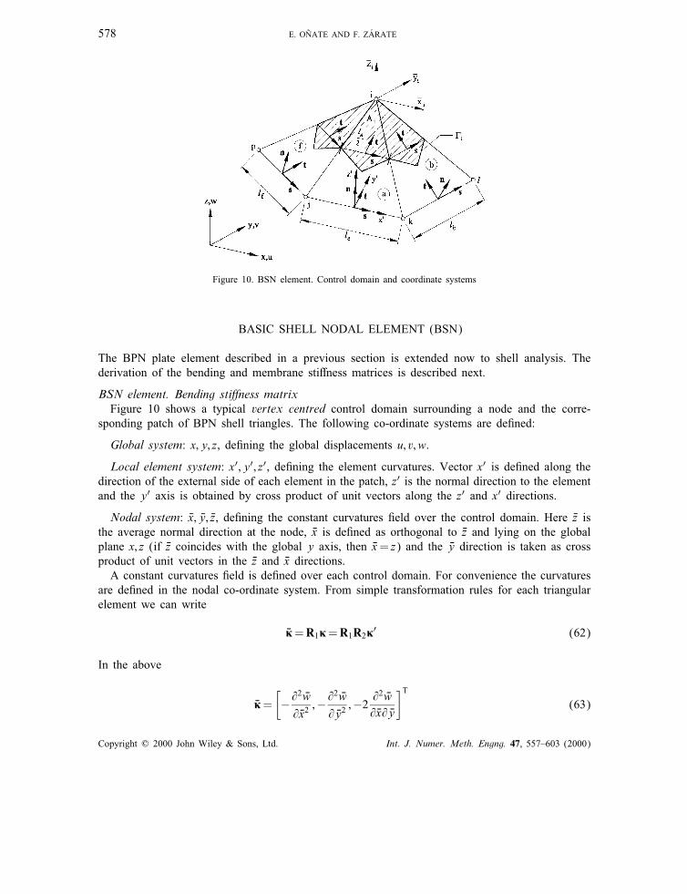
Figure 11. (a) square plate: L = 10, structured mesh, orientation A; (b) square plate: structured mesh, orientation B;(c) circular plate: structured mesh. E = 10·92; � = 0·3 and t = 0·01 in all cases

Note that results for the BPT and BPT1 elements are identical in both cases as expected forregular meshes.The performance of the new rotation free triangles in non-structured meshes was also found to

be remarkable [38]. Results for the central de ection for a clamped plate under a central pointload using a non-structured mesh are shown in Figure 16(a).

Circular plates under uniform and central point loads

Figure 11(c) shows the geometry of the plate and the material properties. Again a number oftests using the BPT, BPT1 and BPN rotation free plate triangles was performed using structuredand non-structured meshes.Numerical results for the central de ection using structured meshes are shown in Figures 17

and 18 for the following cases:

(1) Simple supported circular plate under uniform load and a central point load (Figure 17);(2) Clamped circular plate under a uniform load and a central point load (Figure 18).

The performance of the three rotation free plate elements is excellent. Numerical results werein all cases (with exception of the example of Figure 17(a)) more accurate than those providedby the DKT and the Morley triangles.Note that results for the BPT and BPT1 di�er slightly in this case as the mesh is not regular. No

particular trend in the comparison between the results obtained with the two elements is observed.This favours the use of the BPT element for practical purposes due to its simplicity.Again the performance of all rotation-free plate elements for non-structured meshes was found

to be excellent [38]. A typical example is shown in Figure 16(b).

Skew thin plates under uniform load

Figure 19 shows the typical geometry of the skew plates analysed and the material properties.The following cases are considered.

(1) Bi-clamped 30◦ skewed plate under uniform load (Figure 20)(2) 60◦, 40◦ and 20◦ cantilever skewed plates under uniform load (Figures 21–23).



Figure 12. Central point de ection of a simple supported square plate under uniform load: (a) mesh orientation A; (b) meshorientation B



Figure 13. Central point de ection of a simple supported square plate under central point load: (a) mesh orientation A,(b) mesh orientation B



Figure 14. Central point de ection of a clamped square plate under uniform load: (a) mesh orientation A; (b) meshorientation B



Figure 15. Central point de ection of a clamped square plate under central point load: (a) mesh orientation A; (b) meshorientation B



Figure 16. Central point de ection of clamped square and circular plates under a central point load. Percentage errorin central de ection values obtained with BPT, BPT1 and BPN elements using the non-structured meshes shown.

Geometry and material properties as in Figure 11

Numerical results obtained with BPT, BPT1, BPN, DKT and Morley triangles using structuredmeshes are compared with a �nite di�erence solution reported in [39] and with �nite elementsolutions obtained with the DRM and ELM1 Reissner–Mindlin triangles [13, 20] (Figures 21–23).The performance of the new rotation-free plate elements is also good in all these examples. The

maximum error for a 1000 d.o.f. mesh did not exceed 2·5 per cent in all cases. Obviously thesolution can be improved using mesh adaptivity as shown in [38].

Cylindrical shell under central point load

Figure 24 shows the geometry of the shell, the material properties and the loading. The problemhas been studied with the BST and BSN rotation-free shell triangles using structured and non-structured meshes [38].Figure 24 shows the convergence of the central de ection obtained using structured meshes.

The reference solutions were obtained from [40; 41]. Numerical results for the three rotation-freeshell triangles compare well with those obtained with the DKT-15 [7; 16] element also shown.A plot of the distribution of the bending moment My′ along the central edge AB is shown in

Figure 25.

Cylindrical shell under uniform load

The geometry of the dome known Scordelis–Lo shell [42; 43] is shown in Figure 26. Theconvergence of numerical results for the vertical displacement of the free point B using structured



Figure 17. Central point de ection of a simple supported circular plate: (a) Uniform load, (b) central point load



Figure 18. Central point de ection of a clamped circular plate: (a) Uniform load; (b) central point load



Figure 19. (a) Bi-clamped skewed plate under uniform load; (b) skew cantilever plates under uniform load

Figure 20. Bi-clamped 30◦ skewed plate under uniform load. Convergence of central de ection

meshes is shown in the same �gure. The results obtained with the new rotation-free BST andBSN triangles compare favourably with those obtained with the DKT-15 [7; 16] element. Furtherresults for this problem using non-structured meshes can be found in [38].

Open spherical dome under opposite diametral point loads

The geometry of the dome, the material properties and the mesh is shown in Figure 27. Again thesolution reported here has been obtained using structured meshes. A non-structured mesh analysiscan be found in [38].



Figure 21. 60◦ skew cantilever plate under uniform load: (a) Convergence of de ection of corner point 1; (b) convergence ofde ection of corner point 2



Figure 22. 40◦ skew cantilever plate under uniform load: (a) Convergence of de ection of corner point 1; (b) convergenceof de ection of corner point 2



Figure 23. 20◦ skew cantilever plate under uniform load: (a) Convergence of de ection of corner point 1; (b) convergenceof de ection of corner point 2



Figure 24. Cylindrical shell under central point load. Error in vertical displacement of point A for di�erent structured meshesof BST, BSN and DKT-15 elements

Figure 25. Cylindrical shell under point load. Distribution of My1 bending moment along side B-A for BST, BSN andDKT-15 elements

Figure 27 shows the convergence for the radial displacement of point A obtained with the BPT,BSN and DKT-15 elements. Numerical results converge in all cases to a sti�er solution than thereference value of 0·093 [11; 43]. This well-known defect is due to the appearance of strain energycausing an over sti� exural response commonly known as membrane locking [44]. Methods toelliminate this de�ciency are presented in [8].



Figure 26. Cylindrical shell under uniform load. Convergence of vertical displacement of point B for di�erent structuredmeshes of BST, BSN and DKT-15 elements

Figure 27. Open spherical dome under point load. Error in radial displacement of point A for di�erent structured meshesof BST, BSN and DKT-15 elements

Table I. Open spherical dome. Radial displacement of point A obtained with a structured mesh of 2048triangles using BST, BSN and DKT-15 elements

Rotation-free shell triangles DKT-15

BST BSNNo. of d.o.f wA Error wA Error No. of d.o.f. wA errortriangles triangles

2048 3200 0·0835 10·2 Per cent 0·0821 11·7 2048 5312 0·0798 14·2 Per cent

Some numerical results are shown in Table I. Note that the behaviour of the BST and BSNelements is more accurate than the DKT-15 element for a considerably smaller number of degreesof freedom.



Figure 28. Hyperbolic shell under uniform load. Convergence of vertical displacement of central point for di�erentstructured meshes of BST, BSN and DKT-15 elements

Figure 29. Spherical cup under uniform impulse loading. Geometry, material properties and triangular mesh for analysis withBST, BSN and DKT elements

Hyperbolic shell under uniform load

The geometry of the shell and the material properties are shown in Figure 28. A comparisonof the central de ection values obtained with di�erent structured meshes using BST, BSN andDKT-15 elements is shown in Figure 28 where a reference solution is also shown [45]. Note theaccuracy of less than ' 10 per cent error obtained in all cases for meshes with more than 100d.o.f.

Spherical cap under uniform impulse loading

The last example shows the e�ciency of the new BST and BSN rotation-free shell triangles forexplicit dynamic analysis of shell structures.



Figure 30. (a) Spherical cup under uniform impulse loading. Evolution of central displacement; elastic solution;(b) Elastoplastic solution. Results obtained with BST, BSN, and DKT elements are compared with those obtained

by Bathe [48] and using the explicit dynamic code WHAMS [47]

The problem description and the mesh of 800 triangles (1082 d.o.f.) used to discretize thespherical cap are shown in Figure 29. Fourfold symmetry was used. A uniform load of 600 psiwas applied over the cap as shown. Both elastic and elasto-plastic materials with the materialproperties given in Figure 28 were considered. The results for the central de ection obtained with



the BST and BSN elements are compared in Figures 30(a) and 30(b) to those obtained with theDKT-15 element [46] and with results reported in references [47; 48]. Note the accuracy of thenew rotation-free triangles for both the linear and non-linear solutions.Other examples of the performance of the new rotation-free shell triangles for non-linear dynamic

analysis problems including frictional contact conditions are reported in [49–52].

CONCLUDING REMARKS

A general methodology for deriving rotation-free plate and shell triangles has been described.The two element families here presented result from combining cell centred and cell vertex �nitevolume schemes with �nite element interpolations over triangular elements. The simplest elementsof these two families, i.e. those corresponding to a linear displacement interpolation, have beendescribed in some detail. The resulting plate and shell triangles are simple and inexpensive as theyonly involve translational degrees of freedom as nodal variables.The performace of the new rotation-free plate and shell triangles has been found to be very good

in all cases studied. The elements seen particularly promising for competitive analysis of large-scalenon-linear shell problems typical of sheet metal forming and crash-worthiness situations.

REFERENCES

1. Zienkiewicz OC, Taylor RC., The �nite element method (4th edn), vol. 1. McGraw Hill: New York, 1989.2. Stolarski H, Belytschko T, Lee S-H. A review of shell �nite elements and corotational theories. ComputationalMechanics Advances, 1995; 2(2):125–212.

3. Idelsohn S, Onate E, Dvorkin EN (eds), Proceedings of IACM IV World Congress on Computational Mechanics,CIMNE, Barcelona, 1998.

4. Timoshenko SP. Theory of Plates and Shells. McGraw Hill: New York, 1979.5. Dvorkin EN, Bathe KJ. A continuum mechanics based four node shell element for general non-linear analysis.Engineering Computations, 1984; 1:77–88.

6. Morley LSD. On the constant moment plate bending element. Journal of Strain Analysis 1971; 6:10–14.7. Batoz JL, Bathe KJ, Ho LW. A study of three-node triangular plate bending elements. International Journal forNumerical Methods in Engineering 1980; 15:1771–1812.

8. Carpenter N, Stolarski H, Belytschko T. Improvements in 3-node triangular shell elements. International Journal forNumerical Methods in Engineering 1986; 23:1643–47.

9. Papadopoulos P, Taylor RL. A triangular element based on Reissner-Mindlin plate theory. International Journal forNumerical Methods in Engineering 1988; 30:1029–49.

10. Batoz JL, Lardeur P. A discrete shear triangular nine d.o.f. element for the analysis of thick to very thin plates.International Journal for Numerical Methods in Engineering 1989; 29:1595–1638.

11. Sim�o, JC, Fox DD, Rifai MS. On a stress resultant geometrically exact shell model, Part II: The linear theory:computational aspects. Computer Methods in Applied Mechnics and Engineering, 1989; 73:553–592.

12. Zienkiewicz OC, Taylor RL, Papadopoulos P, Onate E. Plate bending element with discrete constraints: new triangularelements. Computer and Structures 1990; 35:505–522.

13. Auricchio F, Taylor RL. 3 node triangular elements based on Reissner-Mindlin plate theory, Report no. UCB=SEMM-91=04 Dept. Civil Engng. University of California, Berkeley, 1991.

14. Onate E, Zienkiewicz OC, Suarez B, Taylor RL. A methodology for deriving shear constrained Reissner–Mindlin plateelements. International Journal for Numerical Methods in Engineering 1992; 33:345–367.

15. Batoz JL, Katili I. On a simple triangular Reissner-Mindlin plate element based on incompatible modes and discreteconstraints. International Journal for Numerical Methods in Engineering 1992; 26:1603–1632.

16. Batoz JL, Mod�ellisation des structures par �el�ements �ns. Vol. 3 coques, Hermes: Paris, 1992.17. Katili I. A new discrete Kirchho�-Mindlin element based on Mindlin–Reissner plate theory and assumed shear �elds.

Part I: An extended DKT element for thick plate bending analysis. International Journal for Numerical Methods inEngineering 1993; 36:1859–1883.

18. Zienkiewicz OC, Xu Z, Zeng LF, Samuelsson A, Wiberg NE. Linked interpolation for Reissner-Mindlin plate elements.Part I: A simple quadrilateral. International Journal for Numerical Methods in Engineering 1993; 36:3043–3056.



19. Taylor RL, Auricchio F. Linked interpolation for Reissner–Mindlin plate elements. Part II: A simple triangle.International Journal for Numerical Methods in Engineering 1993; 36:3057–3066.

20. Auricchio F, Taylor RL. A triangular thick plate �nite element with an exact thin limit. Finite Elements in Analysisand Design 1995; 19:57–68.

21. Van Keulen F, Bont A, Ernst LJ. Non linear thin shell analysis using a curved triangular element. Computer Methodsin Applied Mechanics and Engineering 1993; 103:315–343.

22. Onate E. A review of some �nite element families for thick and thin plate and shell analysis. In: Recent developmentin �nite element analysis, Hughes TJR, Onate E, Zienkiewicz OC (eds), CIMNE, Barcelona, 1999.

23. Onate E, Z�arate F, Flores F. A simple triangular element for thick and thin plate and shell analysis. InternationalJournal for Numerical Methods in Engineering 1994; 37:2569–2582.

24. Uguraz AC. Stresses in Plates and Shells. McGraw Hill: New York, 1981.25. Nay RA, Utku S. An alternative to the �nite element method. Variational Methods Engineering, 1972; 1.26. Barnes MR. Form �nding and analysis of tension space structure by dynamic relaxation. PhD Thesis, Department of

Civil Engineering, The City University, London, 1977.27. Hampshire JK, Topping BHV, Chan HC. Three node triangular elements with one degree of freedom per node.

Engineering Computations 1992; 9:49–62.28. Phaal R, Calladine CR. A simple class of �nite elements for plate and shell problems. I: Elements for beams and thin

plates. International Journal for Numerical Methods in Engineering 1992; 35:955–977.29. Phaal R, Calladine CR. A simple class of �nite elements for plate and shell problems. II: An element for thin shells

with only translational degrees of freedom. International Journal for Numerical Methods in Engineering 1992; 35:979–996.

30. Yang DY, Jung DW, Song LS, Yoo DJ, Lee JH. Comparative investigation into implicit, explicit and iterativeimplicit=explicit schemes for simulation of sheet metal forming processes. In: NUMISHEET ’93, Makinouchi A,Nakamachi E, Onate E, Wagoner RH (eds), RIKEN: Tokyo 1993; 35–42.

31. Brunet M, Sabourin F. Prediction of necking and wrinkles with a simpli�ed shell element in sheet forming. InProceedings of the International Conference of Metal Forming Simulation in Industry, II, Kr�oplin B (Ed.), 27–48,1994.

32. Rio G, Tathi B, Laurent H. A new e�cient �nite element model of shell with only three degrees of freedom per node.Applications to industrial deep drawing test. In Recent Developments in Sheet Metal Forming Technology, BarataMarques MJM (ed.), 18th IDDRG Biennial Congress, Lisbon, 1994.

33. Onate E, Cervera M. Derivation of thin plate bending elements with one degree of freedom per node. EngineeringComputations 1993; 10:543–561.

34. Onate E, Cervera M, Zienkiewicz OC. A �nite volume format for structural mechanics. International Journal forNumerical Methods in Engineering 1994; 37:181–201.

35. Zienkiewicz OC, Onate E. Finite elements versus �nite volumes. Is there really a choice? In Nonlinear ComputationMechanics. State of the Art Wriggers P, Wagner W (eds), Springer: Berlin, 1991.

36. Idelsohn S, Onate E. Finite volumes and �nite elements: two ‘good friends’. International Journal for NumericalMethods in Engineering 1994; 37:3323–3341.

37. Onate E, Idelsohn S, Zienkiewicz OC, Taylor L. A �nite point method in computational mechanics. Applicationsto convective transport and uid ow. International Journal for Numerical Methods in Engineering 1996; 39:3839–3866.

38. Z�arate F. New �nite elements for plate and shell analysis (in Spanish), PhD Thesis, University Polit�ecnica de Catalunya,Barcelona, 1996.

39. Razzaque A. A program for triangular bending elements with derivative smoothing. International Journal for NumericalMethods in Engineering 1973; 6:333–343.

40. Fl�uge W. Stress in shells. Springer: Berlin, 1960.41. Lindberg GM, Olson MD, Cowper GR. New developments in the �nite element analysis of shells, Quaterly Bulletin,

Vol. 4, Division of Mechanical Engineering and National Aeronautical Establishment, National Research Council ofCanada, 1969.

42. Scordelis AC, Lo KS. Computer analysis of cylindrical shells. Journal of American Concrete Institute 1969; 61:539–561.

43. MacNeal RH, Harder RL. A proposed standard set of problems to test �nite element accuracy. Computer and Structures1985; 20:121–128.

44. Belytschko T, Liu WK, Lam D. Implementation and application of a 9-node Lagrangian shell element with spuriosmode control. Computers and Structures 1985; 20:121–128.

45. Connor JJ, Brebia C, Sti�ness matrix for shallow rectangular shell elements. Journal of Engineering Mechanics.,Divison ASCE, 1967; 93: 43–45.

46. Cendoya P, Explicit dynamic analysis of shells using rotational dof-free triangles. PhD Thesis (in Spanish), UPC,Barcelona, 1996.

47. Bathe KJ, Ramm E, Wilson EL. Finite element formulation for large deformation dynamic analysis. InternationalJournal for Numerical Methods in Engineering 1975; 9:353–386.



48. WHAMS-3D, An Explicit 3D �nite element program. KBS2 Inc: Willow Springs, IL 60480, USA.49. Onate E, Cendoya P, Rojek J, Miquel J. A simple thin shell triangle with translational degrees of freedom for sheet

stamping analysis. Proceedings of the 3rd International Conference on Numerical Simulation of 3D Sheet FormingProcesses (NUMISHEET ’96), Dearbon, Michigan, USA, 29 Sept.–3 Oct., 1996.

50. Onate E, Cendoya P, Rojek J, Miquel J. Non linear explicit dynamic analysis of shell structures using a simple trianglewith translational degrees of freedom only. Proceedings of the International Conference on Computational EngineeringScience (ICES ’97), San Jose, Costa Rica, May 4–9, 1996.

51. Du�et GA, Onate E, Rojek J, Z�arate F. Stampar: A parallel processing approach to sheet stamping simulations. InComputational Plasticity V, Owen DRJ, Onate E, Hinton E (eds), CIMNE, Barcelona, 1997.

52. Jovicevic J, Onate E. Analysis of beams and shells using a rotation-free �nite element–�nite volume formulation.Monograph CIMNE, Barcelona, 1999.


Documents

Rotation-free triangular plate and shell elements - Cimne