Embed Size (px)
Citation preview

University of CambridgeInstitute of Astronomy
A dissertation submitted for the degree ofDoctor of Philosophy
Rotation and magnetismin massive stars
Adrian Thomas Potter
Pembroke College
Under the supervision of Dr. Christopher A. Tout
Submitted to the Board of Graduate Studies10 May, 2012


i
For everyone who helped to get me here

ii

CONTENTS iii
Contents
Contents iii
Declaration vii
Acknowledgements ix
Summary xi
List of Tables xiii
List of Figures xv
1 Introduction 1
1.1 Stellar evolution . . . . . . . . . . . . . . . . . . . . . . . . . . . . . . . . 1
1.1.1 The mechanical equilibrium of stars . . . . . . . . . . . . . . . . . 2
1.1.2 The main sequence . . . . . . . . . . . . . . . . . . . . . . . . . . 3
1.2 Rotation in massive stars . . . . . . . . . . . . . . . . . . . . . . . . . . . 7
1.2.1 Changes in stellar structure . . . . . . . . . . . . . . . . . . . . . 7
1.2.2 The Von Zeipel paradox . . . . . . . . . . . . . . . . . . . . . . . 11
1.2.3 The Kelvin–Helmholtz instability . . . . . . . . . . . . . . . . . . 13
1.2.4 Observations of rotational velocities . . . . . . . . . . . . . . . . . 18
1.2.5 Chemical mixing in massive stars . . . . . . . . . . . . . . . . . . 21
1.3 Stellar magnetism . . . . . . . . . . . . . . . . . . . . . . . . . . . . . . . 22
1.3.1 Observations of magnetism in massive stars . . . . . . . . . . . . 22
1.3.2 Stellar dynamos . . . . . . . . . . . . . . . . . . . . . . . . . . . . 24
1.3.3 Fossil fields . . . . . . . . . . . . . . . . . . . . . . . . . . . . . . 26
1.4 Common envelope evolution . . . . . . . . . . . . . . . . . . . . . . . . . 27
1.5 Dissertation outline . . . . . . . . . . . . . . . . . . . . . . . . . . . . . . 33
2 Modelling rotation and magnetic fields in stars 35
2.1 Stellar structure and evolution . . . . . . . . . . . . . . . . . . . . . . . . 35
2.2 The Cambridge stellar evolution code . . . . . . . . . . . . . . . . . . . . 37
2.3 Modelling stellar rotation . . . . . . . . . . . . . . . . . . . . . . . . . . . 39

iv CONTENTS
2.3.1 Structure equations for rotating stars . . . . . . . . . . . . . . . . 39
2.3.2 Meridional circulation . . . . . . . . . . . . . . . . . . . . . . . . 40
2.3.3 Mass loss with rotation . . . . . . . . . . . . . . . . . . . . . . . . 42
2.3.4 Rotation in convective zones . . . . . . . . . . . . . . . . . . . . . 42
2.3.5 Angular momentum transport . . . . . . . . . . . . . . . . . . . . 42
2.3.6 Numerical implementation of rotation . . . . . . . . . . . . . . . . 43
2.4 Modelling stellar magnetism . . . . . . . . . . . . . . . . . . . . . . . . . 46
2.4.1 Magnetic field evolution . . . . . . . . . . . . . . . . . . . . . . . 46
2.4.2 Angular momentum evolution with a magnetic field . . . . . . . . 48
2.4.3 Magnetic diffusion . . . . . . . . . . . . . . . . . . . . . . . . . . 49
2.4.4 Dynamo model . . . . . . . . . . . . . . . . . . . . . . . . . . . . 50
2.4.5 Magnetic braking . . . . . . . . . . . . . . . . . . . . . . . . . . . 50
2.4.6 Free parameters . . . . . . . . . . . . . . . . . . . . . . . . . . . . 51
2.4.7 Numerical implementation . . . . . . . . . . . . . . . . . . . . . . 52
2.5 Simulating stellar populations . . . . . . . . . . . . . . . . . . . . . . . . 52
3 Comparison of stellar rotation models 55
3.1 Introduction . . . . . . . . . . . . . . . . . . . . . . . . . . . . . . . . . . 55
3.2 Models of stellar rotation . . . . . . . . . . . . . . . . . . . . . . . . . . . 56
3.3 Angular momentum transport . . . . . . . . . . . . . . . . . . . . . . . . 57
3.3.1 Test cases . . . . . . . . . . . . . . . . . . . . . . . . . . . . . . . 57
3.4 Results . . . . . . . . . . . . . . . . . . . . . . . . . . . . . . . . . . . . . 61
3.4.1 Evolution of a 20M� star in cases 1, 2 and 3 . . . . . . . . . . . 61
3.4.2 Effect on Hertzsprung–Russell diagram . . . . . . . . . . . . . . . 65
3.4.3 Nitrogen enrichment . . . . . . . . . . . . . . . . . . . . . . . . . 67
3.4.4 Helium–3 enrichment . . . . . . . . . . . . . . . . . . . . . . . . . 69
3.4.5 Metallicity dependence . . . . . . . . . . . . . . . . . . . . . . . . 69
3.4.6 Surface gravity cut–off . . . . . . . . . . . . . . . . . . . . . . . . 71
3.4.7 Alternative models for convection . . . . . . . . . . . . . . . . . . 74
3.5 Conclusions . . . . . . . . . . . . . . . . . . . . . . . . . . . . . . . . . . 74
4 Model–dependent characteristics of stellar populations 79
4.1 Introduction . . . . . . . . . . . . . . . . . . . . . . . . . . . . . . . . . . 79
4.2 Input physics . . . . . . . . . . . . . . . . . . . . . . . . . . . . . . . . . 80
4.2.1 Case 1 . . . . . . . . . . . . . . . . . . . . . . . . . . . . . . . . . 82
4.2.2 Case 2 . . . . . . . . . . . . . . . . . . . . . . . . . . . . . . . . . 83
4.2.3 Stellar populations . . . . . . . . . . . . . . . . . . . . . . . . . . 84
4.3 Results . . . . . . . . . . . . . . . . . . . . . . . . . . . . . . . . . . . . . 84
4.3.1 The Hertzsprung–Russell diagram . . . . . . . . . . . . . . . . . . 84
4.3.2 Velocity distribution evolution . . . . . . . . . . . . . . . . . . . . 86
4.3.3 The Hunter diagram . . . . . . . . . . . . . . . . . . . . . . . . . 86

CONTENTS v
4.3.4 Effective surface gravity and enrichment . . . . . . . . . . . . . . 89
4.3.5 Recalibration . . . . . . . . . . . . . . . . . . . . . . . . . . . . . 93
4.3.6 Effects of metallicity . . . . . . . . . . . . . . . . . . . . . . . . . 93
4.3.7 Selection effects in the VLT–FLAMES survey . . . . . . . . . . . 98
4.4 Conclusions . . . . . . . . . . . . . . . . . . . . . . . . . . . . . . . . . . 101
5 Stellar evolution with an alpha–omega dynamo 105
5.1 Introduction . . . . . . . . . . . . . . . . . . . . . . . . . . . . . . . . . . 105
5.2 Magnetic rotating model . . . . . . . . . . . . . . . . . . . . . . . . . . . 107
5.3 Results . . . . . . . . . . . . . . . . . . . . . . . . . . . . . . . . . . . . . 108
5.3.1 Magnetic field evolution . . . . . . . . . . . . . . . . . . . . . . . 110
5.3.2 Effect on angular momentum distribution . . . . . . . . . . . . . 113
5.3.3 Mass–rotation relation of the main–sequence field strength . . . . 117
5.3.4 Effect on the Hertzsprung–Russel diagram . . . . . . . . . . . . . 121
5.3.5 The lifetime of fossil fields . . . . . . . . . . . . . . . . . . . . . . 123
5.3.6 Effect on surface composition . . . . . . . . . . . . . . . . . . . . 124
5.3.7 Variation with different parameters . . . . . . . . . . . . . . . . . 128
5.4 Conclusions . . . . . . . . . . . . . . . . . . . . . . . . . . . . . . . . . . 129
6 WD magnetic fields in interacting binaries 133
6.1 Introduction . . . . . . . . . . . . . . . . . . . . . . . . . . . . . . . . . . 133
6.2 CE Evolution and energy constraints . . . . . . . . . . . . . . . . . . . . 134
6.3 Governing equations for magnetic field evolution . . . . . . . . . . . . . . 136
6.4 Numerical Methods . . . . . . . . . . . . . . . . . . . . . . . . . . . . . . 139
6.5 Results . . . . . . . . . . . . . . . . . . . . . . . . . . . . . . . . . . . . . 140
6.5.1 Consequences of CE lifetime . . . . . . . . . . . . . . . . . . . . . 141
6.5.2 Effect of randomly varying the magnetic field orientation . . . . . 146
6.6 Conclusions . . . . . . . . . . . . . . . . . . . . . . . . . . . . . . . . . . 152
7 Conclusions 155
7.1 Populations of rotating stars . . . . . . . . . . . . . . . . . . . . . . . . . 155
7.2 Populations of magnetic, rotating stars . . . . . . . . . . . . . . . . . . . 158
7.3 Highly magnetic white dwarfs . . . . . . . . . . . . . . . . . . . . . . . . 159
7.4 Future work . . . . . . . . . . . . . . . . . . . . . . . . . . . . . . . . . . 159
A Stellar structure derivations 161
A.1 The structure parameter, fP . . . . . . . . . . . . . . . . . . . . . . . . . 161
A.2 The structure parameter, fT . . . . . . . . . . . . . . . . . . . . . . . . . 163
A.3 The Von Zeipel Theorem . . . . . . . . . . . . . . . . . . . . . . . . . . . 164
Bibliography 167

vi CONTENTS

vii
Declaration
I hereby declare that my dissertation entitled Rotation and magnetism in mas-sive stars is not substantially the same as any that I have submitted for a degreeor diploma or other qualification at any other university. I further state thatno part of my thesis has already been or is being concurrently submitted forany such degree, diploma or other qualification. This dissertation is the resultof my own work and includes nothing which is the outcome of work done incollaboration except where specifically indicated in the text. Those parts whichhave been published or accepted for publication are:
• Material from chapter 1 is largely intended as a literature review and sodraws heavily on the references contained therein. Material from section 1.4was submitted for the Certificate of Postgraduate Study to the Universityof Cambridge.
• Material from chapters 2 and 3 has been published as: Potter A. T.,Tout C. A. and Eldridge J. J., 2012, “Towards a unified model of stellarrotation”, Monthly Notices of the Royal Astronomical Society, 419, 788-759and was completed in collaboration with these authors.
• Material from chapters 2 and 4 has been accepted for publication as: Pot-ter A. T., Brott I. and Tout C. A., “Towards a unified model of stellar ro-tation II: Model-dependent characteristics of stellar populations”, MonthlyNotices of the Royal Astronomical Society and was completed in collabo-ration with these authors.
• Material from chapters 2 and 5 has been accepted for publication as: Pot-ter A. T., Chitre S. M. and Tout C. A., “Stellar evolution of massive starswith a radiative alpha–omega dynamo”, Monthly Notices of the Royal As-tronomical Society and was completed in collaboration with these authors.
• Material from chapter 6 has been published as: Potter A. T. and Tout C. A.,2010, “Magnetic field evolution of white dwarfs in strongly interacting bi-nary star systems”, Monthly Notices of the Royal Astronomical Society,402, 1072-1080 and was completed in collaboration with that author.
This dissertation contains fewer than 60, 000 words.
Adrian Potter
June 2, 2012

viii DECLARATION

ix
Edmund: It’s taken me seven years, and it’s
perfect... My magnum opus, Baldrick. Every-
body has one novel in them, and this is mine.
Baldrick: And this is mine. My magnificent
octopus.
(Blackadder the Third, Ink and Incapability) Acknowledgements
For this piece of work I am indebted to the invaluable help and support of
countless people over the past four years. Without their time and effort none
of this work would have been possible.
First and foremost I would like to give the greatest of thanks to my supervisor,
Christopher Tout. His hard work, knowledge and guidance have been an abso-
lutely essential for driving this work forwards and I am thoroughly grateful. I
am also particularly thankful for the support of John Eldridge who stepped in
to fill the void whilst Christopher was on sabbatical. Not only that but his firm
knowledge of the Cambridge stellar evolution code has allowed me to overcome
countless hurdles. I would also like to thank Ines Brott and Shashikumar Chitre
for their ongoing support.
The success of a PhD is dependent on all of those people behind the scenes who
make things possible. Firmly at the top of that list is Andrea Kuesters who has
always been there when I needed her the most. I have always been able count
on her regardless of what life sent my way and for that I am eternally grateful.
More than that we’ve had some fantastic times and even when she tried to
break my hand one Christmas, I treasure every moment we’ve spent together. I
also couldn’t have asked for a better year group at the Institute of Astronomy.
Amy, Becky, Ryan, Warrick, Steph, Alex, Jon, James, other James, Dom and
Yin-Zhe, you’ve been fantastic, thank you. I’d also like to thank Chrissie, Amy,
Natasha, Barny, Sam, Mark C, James, Samantha, Mark W, Simon, Bahar,
Sophie and Lucy for all the great times during the past four years. In addition
I’d like to thank Sian Owen, Margaret Harding and Becky Coombs for their
tireless administrative efforts. My family have also been a constant source of
support. They shouldered the financial burden of my degrees and have always
been just a phone call away whenever I needed them.
Finally I’d like to give my thanks to Christine whose love, support and en-
couragement has been unwavering. Her time and understanding has been so
important in helping me to cope with pressure of finishing my eight years in
Cambridge and I’m very thankful for everything she’s given me.

x ACKNOWLEDGEMENTS

xi
...so smart it’s got a PhD from Cambridge.
(Blackadder Goes Forth, Private Plane)
Summary
Rotation has a number of important effects on the evolution of stars. Apart from struc-
tural changes because of the centrifugal force, turbulent mixing and meridional circulation
can dramatically affect a star’s chemical evolution. This leads to changes in the surface
temperature and luminosity as well as modifying its lifetime. Rotation decreases the
surface gravity, causes enhanced mass loss and leads to surface abundance anomalies
of various chemical isotopes all of which have been observed. The replication of these
physical effects with simple stellar evolution models is very difficult and has resulted in
the use of numerous different formulations to describe the physics. We have adapted the
Cambridge stellar evolution code to incorporate a number of different physical models
for rotation, including several treatments of angular momentum transport in convection
zones. We compare detailed grids of stellar evolution models along with simulated stellar
populations to identify the key differences between them. We then consider how these
models relate to observed data.
Models of rotationally-driven dynamos in stellar radiative zones have suggested that
magnetohydrodynamic transport of angular momentum and chemical composition can
dominate over the otherwise purely hydrodynamic processes. If this is the case then a
proper consideration of the interaction between rotation and magnetic fields is essen-
tial. We have adapted our purely hydrodynamic model to include the evolution of the
magnetic field with a pair of time-dependent advection–diffusion equations coupled with
the equations for the evolution of the angular momentum distribution and stellar struc-
ture. This produces a much more complete, though still reasonably simple, model for the
magnetic field evolution. We consider how the surface field strength varies during the
main-sequence evolution and compare the surface enrichment of nitrogen for a simulated
stellar population with observations.
Strong magnetic fields are also observed at the end of the stellar lifetime. The surface
magnetic field strength of white dwarfs is observed to vary from very little up to 109G.
As well as considering the main-sequence evolution of magnetic fields we also look at how
the strongest magnetic fields in white dwarfs may be generated by dynamo action during
the common envelope phase of strongly interacting binary stars. The resulting magnetic
field depends strongly on the electrical conductivity of the white dwarf, the lifetime of the
convective envelope and the variability of the magnetic dynamo. We assess the various
energy sources available and estimate necessary lifetimes of the common envelope.

xii SUMMARY

LIST OF TABLES xiii
List of Tables
3.1 The diffusion coefficients used by each of the different cases examined in
chapter 3 . . . . . . . . . . . . . . . . . . . . . . . . . . . . . . . . . . . . 58
4.1 The properties of the single–aged stellar populations used in section 4.3 . 83
5.1 The variation of magnetic stellar evolution owing to variation in parameters
for magnetic field evolution . . . . . . . . . . . . . . . . . . . . . . . . . 128
6.1 Residual surface magnetic field strengths generated by a varying external
field . . . . . . . . . . . . . . . . . . . . . . . . . . . . . . . . . . . . . . 151
6.2 Residual surface field strengths generated by an external field of strength
B0 which reorients at intervals of 109 s . . . . . . . . . . . . . . . . . . . 152

xiv LIST OF TABLES

LIST OF FIGURES xv
List of Figures
1.1 Schematic of the two principal forces acting in a hydrostatic star . . . . . 2
1.2 HR diagram for the main–sequence evolution for a range of masses of non–
rotating stars . . . . . . . . . . . . . . . . . . . . . . . . . . . . . . . . . 6
1.3 High–resolution image of the visible surface of the rapidly rotating star
Altair . . . . . . . . . . . . . . . . . . . . . . . . . . . . . . . . . . . . . 9
1.4 The distortion of stars with different rotation rates calculated using the
Roche Model . . . . . . . . . . . . . . . . . . . . . . . . . . . . . . . . . 10
1.5 Contours of constant potential in a rotating star calculated using the Roche
Model . . . . . . . . . . . . . . . . . . . . . . . . . . . . . . . . . . . . . 12
1.6 Van Gogh’s “La Nuit Etoilee” . . . . . . . . . . . . . . . . . . . . . . . . 14
1.7 Numerical simulation of the Kelvin–Helmholtz instability . . . . . . . . . 15
1.8 Rotational broadening of absorption lines in stellar spectra . . . . . . . . 19
1.9 Rotational velocity distribution of B–stars . . . . . . . . . . . . . . . . . 20
1.10 An example of the Roche potential for two orbiting point masses . . . . . 29
1.11 Reconstructed values of the common envelope efficiency parameter for a
number of systems . . . . . . . . . . . . . . . . . . . . . . . . . . . . . . 32
3.1 Terminal age main sequence composition of a 20 M� rotating star . . . . 61
3.2 Zero age main sequence properties for the angular momentum distribution
in a 20 M� rotating star . . . . . . . . . . . . . . . . . . . . . . . . . . . 63
3.3 Terminal age main sequence properties of the angular momentum distri-
bution in a 20 M� rotating star . . . . . . . . . . . . . . . . . . . . . . . 64
3.4 Hertzsprung–Russell diagram for a range of stellar masses and rotation rates 65
3.5 Hertzsprung–Russell diagram for various masses of star rotating at 300 km s−1
for a number of different models . . . . . . . . . . . . . . . . . . . . . . . 66
3.6 Hunter diagrams for different stellar masses for a number of different phys-
ical models . . . . . . . . . . . . . . . . . . . . . . . . . . . . . . . . . . . 68
3.7 Helium–3 enrichment variation with surface rotation for 10 M� and 60 M�stars for a number of different physical models . . . . . . . . . . . . . . . 70
3.8 Hunter diagrams at low metallicity for different stellar masses for a number
of different physical models . . . . . . . . . . . . . . . . . . . . . . . . . . 72

xvi LIST OF FIGURES
3.9 Effective gravity variation with surface velocity for 10 M� and 60 M� low–
metallicity stars for a number of different physical models . . . . . . . . . 73
3.10 Angular velocity distributions for 60 M� stars initially rotating at 300 km s−1
for different models of angular momentum transport in convective zones . 75
3.11 Hunter diagrams for 10 M� and 60 M� stars for different models of angular
momentum transport in convective zones . . . . . . . . . . . . . . . . . . 76
4.1 Grid of models for simulating stellar populations in chapter 4 . . . . . . . 82
4.2 Hertzsprung–Russell diagrams for stellar populations at age 2 × 10⁷ yr for
different physical models . . . . . . . . . . . . . . . . . . . . . . . . . . . 85
4.3 Velocity distributions of stellar populations at age 2 × 10⁷ yr for different
physical models . . . . . . . . . . . . . . . . . . . . . . . . . . . . . . . . 87
4.4 Hunter diagrams for stellar populations at various ages for different phys-
ical models . . . . . . . . . . . . . . . . . . . . . . . . . . . . . . . . . . . 88
4.5 Hunter diagrams for stellar population under the assumption of continuous
star formation for different physical models . . . . . . . . . . . . . . . . . 90
4.6 Relation between the mass and surface gravity in a simulated stellar pop-
ulation of age 107 yr . . . . . . . . . . . . . . . . . . . . . . . . . . . . . . 91
4.7 Surface nitrogen enrichment against effective surface gravity for popula-
tions at a range of ages for different physical models . . . . . . . . . . . . 92
4.8 Surface nitrogen enrichment against effective surface gravity of simulated
populations of stars with continuous star formation for different physical
models . . . . . . . . . . . . . . . . . . . . . . . . . . . . . . . . . . . . . 94
4.9 Hunter diagrams for simulated stellar populations in case 2b . . . . . . . 95
4.10 Surface nitrogen enrichment against mass for simulated stellar populations
with continuous star formation for different physical models . . . . . . . 96
4.11 Hunter diagrams for simulated stellar populations at LMC metallicity . . 97
4.12 Hunter diagrams for simulated stellar populations undergoing continuous
star formation with different physical models . . . . . . . . . . . . . . . . 99
4.13 Distribution of masses in a simulated stellar population at LMC metallicity 100
5.1 Grid of models used in section 5.3 . . . . . . . . . . . . . . . . . . . . . . 109
5.2 Magnetic field evolution in a 5 M� star initially rotating at 300 km s−1
without magnetic braking . . . . . . . . . . . . . . . . . . . . . . . . . . 111
5.3 Evolution of the magnetic field in a 5 M� star initially rotating at 300 km s−1
with magnetic braking . . . . . . . . . . . . . . . . . . . . . . . . . . . . 112
5.4 Evolution of the surface magnetic field strengths in rotating stars of various
masses . . . . . . . . . . . . . . . . . . . . . . . . . . . . . . . . . . . . . 114
5.5 Turbulent diffusivities governing angular momentum transport in a mag-
netic, rotating 5 M� star . . . . . . . . . . . . . . . . . . . . . . . . . . . 115

LIST OF FIGURES xvii
5.6 Evolution of the angular momentum distribution in a rotating, magnetic
5 M� star . . . . . . . . . . . . . . . . . . . . . . . . . . . . . . . . . . . 116
5.7 Main–sequence magnetic field strengths for ZAMS stars with varying masses
and rotation rates . . . . . . . . . . . . . . . . . . . . . . . . . . . . . . . 118
5.8 Masses and magnetic field strengths of stars in a synthetic stellar popula-
tion with ongoing star formation . . . . . . . . . . . . . . . . . . . . . . . 119
5.9 Hertzsprung–Russell diagram for magnetic, rotating stars of various masses 121
5.10 Evolution of the magnetic field strength of 5 M� in the absence of dynamo
regeneration . . . . . . . . . . . . . . . . . . . . . . . . . . . . . . . . . . 122
5.11 Hunter diagram for LMC stars observed in the VLT–FLAMES survey of
massive stars . . . . . . . . . . . . . . . . . . . . . . . . . . . . . . . . . 124
5.12 Hunter diagram for a population of stars drawn from the grid of models
shown in Fig. 5.1 . . . . . . . . . . . . . . . . . . . . . . . . . . . . . . . 125
5.13 Relation between field strength, mass and rotation rate in a simulated
population of stars according to the observational constraints of the VLT–
FLAMES survey . . . . . . . . . . . . . . . . . . . . . . . . . . . . . . . 126
6.1 Radial magnetic field strength at 0.99 of the stellar radius for a white dwarf
embedded in a uniform vertical field . . . . . . . . . . . . . . . . . . . . . 142
6.2 Radial magnetic field strength at 0.9 of the stellar radius for a white dwarf
embedded in a uniform vertical field . . . . . . . . . . . . . . . . . . . . . 143
6.3 Meridional magnetic field strength at 0.99 of the stellar radius for a white
dwarf embedded in a uniform vertical magnetic field . . . . . . . . . . . . 144
6.4 Meridional magnetic field strength at 0.9 of the stellar radius for a white
dwarf embedded in a uniform vertical magnetic field . . . . . . . . . . . . 145
6.5 Behaviour of the transfer efficiency factor, Q(γ) as described in section 6.5.2.147
6.6 Form of the induced field within the DC with spatially uniform diffusivity
and varying external field . . . . . . . . . . . . . . . . . . . . . . . . . . 148
6.7 Decay of the magnetic field of a WD upon removal of a constant external
magnetic field . . . . . . . . . . . . . . . . . . . . . . . . . . . . . . . . . 150

xviii LIST OF FIGURES

1
Focus on the journey, not the destination. Joy
is found not in finishing an activity but in do-
ing it. (Greg Anderson)
1Introduction
The study of the effects of rotation on stars is notoriously difficult because of the challenge
to introduce them in a consistent yet sufficiently simple way. Rotation’s strong connection
with the evolution of magnetic fields through dynamo mechanisms means that a great
deal of interesting behaviour arises from their introduction into stellar models. Rotation
and magnetic fields are present in almost all areas of astrophysics at all scales and are
so very deserving of attention. Massive stars are of particular interest because they are
largely responsible for driving the heavy element chemical evolution of the Universe. They
are far hotter and more luminous than our own Sun and burn through their nuclear fuel
much faster. During the late stages of their evolution, many of the heavier elements that
are so important to us on Earth, are formed and at the end of their lives they explode
in huge supernovae, scattering their ashes over huge distances. The remnants of these
explosions eventually begin to collapse again to form new stars and planets. Rotation
and magnetic fields not only affect the structure of stars but also the way in which they
evolve. Understanding how rotation and magnetic fields affect stars is therefore of great
importance for understanding how the Universe evolves as a whole.
1.1 Stellar evolution
At its simplest level, stellar evolution is the study of why stars exist and how they change
over time. The subject has a long history and beyond the fairly straightforward basic
principles, a huge number of subtle and interesting effects have been identified that cause
a plethora of fascinating behaviours. In this work we focus on two of these, rotation and
magnetism.

2 CHAPTER 1. INTRODUCTION
Figure 1.1: Schematic diagram showing the forces of gravity and pressure acting in a star in hydrostaticequilibrium.
1.1.1 The mechanical equilibrium of stars
Stars are incredible objects. They power the Universe through nuclear fusion and make
life possible through the formation of heavy elements. Yet basic models of stars can be
constructed from extremely simple principles. At each point in a star, the stellar material
is being acted on by two major forces.
• Gravity: Stars are extremely massive objects. The mass of the Sun is 2 × 1030 kg.
By comparison, the mass of the Earth is 6×1024 kg, roughly a million times smaller.
Because the gravitational pull of an object is proportional to its mass, the surface
gravity of the Sun is roughly 28 times stronger than on Earth1. In a more extreme
case, white dwarfs, which are stars that have expended their nuclear fuel, have
a diameter comparable to the Earth and mass comparable to the Sun. In these
stars, the surface gravity can be millions of times greater than on Earth. Gravity
is extremely important in stars and is constantly pulling all material towards the
centre.
• Pressure: This is the combination of the outward force due to the gas and radiation
within a star. Pressure is a measure of the overall outward force exerted by ions,
electrons and even photons in a material. A gas (or alternatively a liquid or plasma)
is made up of atoms undergoing rapid, random motions. For any enclosed gas, the1The surface gravity of the Sun is not a million times larger than on Earth because the Sun has a much larger radius.

1.1. STELLAR EVOLUTION 3
surface of the enclosure must exert a force on any atoms that collide with it to
prevent them from passing through. The sum of the force from all of the collisions
is called pressure. In a star material isn’t enclosed in a container but atoms in the
gas do collide with each other. Imagine a completely permeable boundary in a star.
Atoms cross in both directions. If more atomic collisions occur below the boundary
(i.e. the pressure is higher) than above it then more atoms will be ejected in the
upwards direction than are deflected downwards. There is therefore a tendency
for a net upward transfer of momentum, or in other words the material below the
boundary exerts an upwards force on the material above the boundary. Hence we are
not so much interested in the total pressure in a star but how the pressure changes
at different levels.
Because gravity and pressure both act isotropically (i.e. equally in all directions) stars
tend towards spherical symmetry2.
The balance of these two forces, pressure acting outwards and gravity acting towards
the centre, keeps stars in perfect equilibrium. We call this situation hydrostatic equilib-
rium, illustrated in Fig. 1.1. In stars this equilibrium is, thankfully, extremely stable.
The change caused by the introduction of the centrifugal force3, which arises because of
rotation, is one of the main focuses of this work.
1.1.2 The main sequence
Stars proceed through a number of important stages of evolution during their lifetimes.
Stars are formed from protostellar clouds which collapse under their own gravity, this
stage of evolution is commonly referred to as the pre–main sequence. Eventually the
internal pressure and temperature become large enough to ignite the fusion of hydrogen
to helium. This is the start of the main sequence. Beyond this point, nuclear fusion
becomes the primary energy source for the star. The fusion of hydrogen into helium halts
the collapse of the star which then remains in a stable, quiescent state over a time period
varying between a few million and many billions of years depending on the mass of the
star. Eventually a star burns through all of the hydrogen in the core. When the central
hydrogen abundance reaches zero, the star starts to rapidly expand. This marks the end
of the main sequence and the star transitions into the various phases of giant evolution.
Hydrogen is converted into helium through two primary mechanisms, the pp chain
and the CNO cycle. Stars begin their lives composed of around one quarter helium and
three quarters hydrogen by mass. There are also small quantities of heavier elements
often present (in particular carbon, nitrogen and oxygen, which are produced in the late
stages of the evolution of massive stars). The rate of the CNO cycle depends strongly on
how abundant these elements are.2I recall one departmental meeting where we spent over an hour discussing the fundamental reason why stars are
spherical.3A force which does exist! We refer the reader to http://xkcd.com/123/.

4 CHAPTER 1. INTRODUCTION
The pp chain dominates the nuclear reactions at temperatures lower than around
2 × 10⁷ K and is split into three different branches. The first few reactions of each chain
are the same. They start with the formation of a deuterium nucleus, 2H, from two
hydrogen nuclei
1H +1 H →2 H + e+ + ν (1.1)
and release a positron, e+, which annihilates quickly with an electron, e, and a neutrino,
ν. Another proton then fuses with the deuterium nucleus so that
1H +2 H →3 He + γ, (1.2)
releasing an energetic photon, γ. From this point on the reaction chains are different.
• ppI: This reaction dominates between around 107 K and 1.4× 10⁷ K. In this process,
two 3He nuclei fuse to produce 4He,
3He +3 He →4 He + 21H + γ. (1.3)
The ppI chain produces 26.2 MeV per 4He nucleus produced.
• ppII: This reaction dominates between around 1.4 × 10⁷ K and 2.3 × 10⁷ K. The
reactions of the ppII chain are
3He +4 He →7 Be + γ, (1.4)
7Be + e− →7 Li + ν, (1.5)
and7Li +1 H → 24He. (1.6)
The ppII chain produces 25.7 MeV of energy per 4He nucleus.
• ppIII: In this branch of the chain, 7Be is produced as in the ppII chain but the
reaction progresses as
7Be +1 H →8 Be∗ + γ, (1.7)
8Be∗ →8 Be + e+ + ν + γ, (1.8)
and8Be → 24He, (1.9)
where 8Be∗ is an unstable isotope of beryllium. This branch of the reaction is
important only when the temperature is greater than 2.3×10⁷ K and generates 19.3
MeV of energy.

1.1. STELLAR EVOLUTION 5
If the temperature exceeds 2×10⁷ K then nuclear reactions are dominated by the CNO
cycle which generates 23.8 MeV of energy per 4He nucleus. The reactions of these cycles
are
12C +1 H →13 N + γ, (1.10)
13N →13 C + e+ + ν, (1.11)
13C +1 H →14 N + γ, (1.12)
14N +1 H →15 O + γ, (1.13)
15O →15 N + e+ + ν, (1.14)
and15N +1 H →12 C +4 He + γ. (1.15)
Evidently the nuclear processes that cause the evolution of a star across the main
sequence are very dependent on the temperature of the stellar material, this is mainly
influenced by the mass of the star. Stars of different masses evolve quite differently. In
this piece of work we focus solely on massive stars. The exact definition of what massive
means varies between authors but we consider such stars to have convective cores and
radiative outer envelopes. This applies to all stars more massive than approximately
1.2 M�. Typically we refer to intermediate–mass stars as stars with masses between
1.2 M� and 10 M�. High–mass stars are those stars more massive than 10 M�. We show
the main–sequence evolution in the Hertzsprung–Russell diagram for stars with a range
of masses in Fig. 1.2. The Hertzsprung–Russell diagram relates the temperature and
luminosity evolution of stars.
Of particular importance to us in this work is the main–sequence lifetime of a star.
A star that lives for longer has more time for rotational mixing to transport material
between the core and the surface. In addition, stars that live for longer, have more time
to be spun down by magnetic braking and there is more time for the magnetic field to
decay. Any difference in the stellar lifetime therefore has serious consequences for the
evolution of the angular momentum distribution and the magnetic field. As shown in
Fig. 1.2, the luminosity of a main–sequence star increases rapidly with mass. This is
because of the higher temperature and pressure in the cores of massive stars and the
lower opacity of their outer envelopes. In fact, the stellar luminosity increases roughly
as a power law such that L ∝ M3.5 where L is the stellar luminosity and M is the
stellar mass. This power law breaks down above around M ≈ 50 M� because the opacity
in this range is dominated by electron scattering which is not strongly dependent on
temperature. The lifetime of a star depends on how rapidly it burns through its fuel (i.e.
the luminosity) and how much fuel there is to burn. The latter increases in proportion to
the stellar mass. The main–sequence lifetime therefore varies as τms ∝ M−2.5. Therefore,

6 CHAPTER 1. INTRODUCTION
2
3
4
5
6
3.9 4 4.1 4.2 4.3 4.4 4.5 4.6 4.7
log 1
0(L
/L�
)
log10(Teff/K)
3M�5M�
10M�20M�40M�60M�
100M�
Figure 1.2: The Hertzsprung–Russell diagram for the main–sequence evolution of non–rotating solar–metallicity stars for a range of initial masses between 3M�and 100M�. The horizontal axis is for theeffective surface temperature, Teff , and the vertical axis is for the stellar luminosity, L.

1.2. ROTATION IN MASSIVE STARS 7
the main–sequence lifetime of a star is far shorter for more massive stars.
In this work we focus on the main–sequence evolution of stars. Whilst models of
rotation and magnetic fields have often been extended on to the giant branch, it is much
more difficult to get a convergent model owing to the emergence of convective shells. The
dramatic change in the mechanism for angular momentum transport across these shells
means that models tend to be far less stable than their main–sequence counterparts.
A consequence is that, whilst models might progress to further stages of evolution, the
progress of a model is likely to be very dependent on the stellar mass and the particular
stages of evolution the model has to traverse.
1.2 Rotation in massive stars
Stars rotate because it is actually quite hard for them not to. Every object in our own
Solar System is rotating; the Earth, the Sun, the planets, the asteroids and the moons.
So it is reasonable to expect that objects beyond the Solar System also rotate which is
indeed what we observe. Stellar rotation arises from two simple ideas, turbulence in the
interstellar medium and conservation of angular momentum. Stars form from giant clouds
of gas that collapse under their own gravity. This material has large–scale turbulence and
so different fluid parcels are moving in different directions. When a section of the cloud
starts to collapse, it is therefore highly probable that the material has non–zero total
angular momentum, an average rotation in one particular direction around the centre.
The amount of angular momentum the cloud has varies greatly because of the random
nature of turbulence. As the cloud collapses, it retains its total angular momentum
and, much as an ice skater does when she4 draws in her arms, rotates at an increasingly
rapid rate the further it contracts. The gas almost certainly sheds some of its angular
momentum through mass loss from the system during the various stages of star formation
but almost all of the angular momentum would have to be lost from the system for the
star to have minimal rotation. For a review of the star formation process we direct the
reader to McKee and Ostriker (2007). Rotation in stars is therefore a rather normal
feature of their structure. One of the key questions in this work is how fast does a star
need to be rotating before it has a significant effect on the structure and evolution and,
when it does, what exactly are those effects.
1.2.1 Changes in stellar structure
Owing to the Earth’s rotation, it is over 20 km wider at the equator than it is from pole to
pole. The same effect happens in stars except, in a high proportion of cases, the rotation
is sufficiently rapid that the effect is far more pronounced. In fact the equatorial radius
can approach 1.5 times the polar radius. This figure not only comes from theoretical
models but also from long–baseline interferometric observations of the rapidly rotating
4This choice of pronoun is because it specifically refers to Christine Yallup.

8 CHAPTER 1. INTRODUCTION
stars Achernar (Carciofi et al., 2008) and Altair (Peterson et al., 2006). A map of the
visible surface of Altair by Peterson et al. (2006) is shown in Fig. 1.3. In this figure, the
distortion to the shape of the star is clearly visible. It is also notable that the star is
hotter at the poles than at the equator. We discuss this further in section 1.2.2.
We can approximate the distortion of stars owing to rotation with a number of simple
models. One of the most common models is that of McLaurin Spheroids which assumes
that the star is a body of constant density with uniform rotation velocity. The other
is the Roche model which assumes the gravitational potential is that of the mass of
the star concentrated at the centre. Typically the second approximation is a better fit
to simulations and observations owing to the strong density gradient in stars. For an
introduction to McLaurin Spheroids we direct the reader to section 41.1 of Kippenhahn
and Weigert (1994).
In the Roche model we assume a spherically symmetric gravitational potential
Φgrav = −GM
r(1.16)
where G is the gravitational constant, M is the mass of the star and r is the distance
from the centre. This is the gravitational potential of mass M concentrated at the origin.
If the star rotates as a solid body then we can represent the potential of the centrifugal
force by
Φrot = −1
2s2Ω2 (1.17)
where s is the perpendicular distance from the rotation axis and Ω is the angular velocity.
Let z be the perpendicular distance from the equatorial plane so that r2 = s2 + z2. The
total potential is then
Φ = Φgrav + Φrot = − GM√s2 + z2
− s2Ω2
2. (1.18)
As in section 1.4 the stellar surface is expected to lie along lines of constant potential,
Φ = constant. For Roche models, the critical rotation rate, above which the star becomes
unbound, is given by
Ωcrit =
√8GM
27R3p
(1.19)
where Rp is the polar radius. Fig. 1.4 shows how the shape of stars in the Roche Model
changes with rotation rate. We note that stars rotating at 80% of their critical rotation
rate still only have an equatorial radius which is approximately 14% larger than their
polar radius.

1.2. ROTATION IN MASSIVE STARS 9
Figure 1.3: A false–colour rendering of the visible surface of the rapidly rotating star, Altair, fromPeterson et al. (2006). Red indicates lower luminosity and blue indicates higher luminosity. It is alsoindicative of the temperature which ranges from 8,740 K at the poles to 6,890 K at the equator.

10 CHAPTER 1. INTRODUCTION
0.0 0.2 0.4 0.6 0.8 1.0 1.2 1.4
0.0
0.2
0.4
0.6
0.8
1.0
1.2
1.4
x
Rp
y Rp
Figure 1.4: The distortion of stars rotating at different rates calculated with the Roche Model. Thecontours are for different values of ζ = Ω
Ωcrit; ζ = 0 (black), ζ = 0.2 (green), ζ = 0.4 (red), ζ = 0.6 (cyan),
ζ = 0.8 (orange), ζ = 1.0 (blue). The degree of distortion is reasonably small even for rotation rates upto 80% of critical rotation. For very high rotation rates the ratio of the equatorial radius to the polarradius tends to 1.5.

1.2. ROTATION IN MASSIVE STARS 11
1.2.2 The Von Zeipel paradox
The condition for radiative equilibrium outside burning regions in a hydrostatic star is
such that the divergence of the radiative flux, F , is 0 (i.e. ∇ · F = 0). This condition
ensures that the amount of heat flux is conserved as it passes through an arbitrary fluid
parcel, or rather that no energy is either created or destroyed as it is transported through
the star. Von Zeipel (1924) considered how radiative equilibrium would be affected by
rotation and concluded that a rotating, hydrostatic star could not simultaneously be in
radiative equilibrium. This is commonly known as the Von Zeipel paradox. For a complete
description we direct the reader to Tassoul (1978). We go through a basic derivation here.
The thermal flux at some point in a star is given by
F = −4acT 3
3κρ∇T, (1.20)
where a = 7.5646×10⁻¹⁵erg cm−3 K−4 is the radiation–density constant, c is the speed of
light, T is the temperature, κ is the opacity and ρ is the density. All of these quantities
can be written in terms of the total potential, Φ, which includes the force of gravity and
rotation such that
F =
(−4a3T 3
3κρ
dT
dΦ
)∇Φ = f(Φ)∇Φ, (1.21)
where f(Φ) is some unknown function of the potential. The radiative flux is therefore
perpendicular to contours of constant Φ. If we calculate the divergence of F from equation
(1.21) we find
∇ · F = f ′(Φ)(∇Φ)2 + f(Φ)∇2Φ. (1.22)
From Poisson’s equation we know that ∇2Φ = 4πGρ − 2Ω2 where G is the gravitational
constant and Ω is the angular velocity which is also constant along lines of constant
Φ. However, ∇Φ is not constant at different co–latitudes, the contours of constant Φ
in a rotating star are closer together at the poles than they are at the equator. This is
illustrated in Fig. 1.5. Therefore the right–hand side of equation (1.22) is non–zero and
radiative equilibrium cannot be established.
Von Zeipel (1924) took this further and established a relation between the effective
gravity and effective temperatures; Teff(Ω, θ) ∝ geff(Ω, θ)14 . This is Von Zeipel’s theorem,
derivations of which can be found in Tassoul (1978) and Maeder (2009). A brief derivation
is given in appendix A.3. On the stellar surface the effective gravity is stronger at the
poles than at the equator owing to the action of the centrifugal force so we similarly
expect the effective surface temperature to be higher at the poles than at the equator.
This is exactly the observation of rapidly rotating star Altair as shown in Fig. 1.3.
As rotation breaks the radiative equilibrium within the star, additional processes must
occur in order to bring the star back into equilibrium. As a result of the Von Zeipel

12 CHAPTER 1. INTRODUCTION
0.0 0.2 0.4 0.6 0.8 1.0 1.2 1.4
0.0
0.2
0.4
0.6
0.8
1.0
1.2
1.4
x
Rp
y Rp
Figure 1.5: The shape of contours of constant potential in a star rotating at 99% of its critical rotationrate calculated using the Roche Model. The contours are for different values of the potentail, Φ. Giventhat the potential at the surface of the star is Φsurf the contours as for, Φ = Φsurf (black), Φ = 1.2Φsurf
(green), Φ = 1.4Φsurf (red), Φ = 1.6Φsurf (cyan), Φ = 1.8Φsurf (orange), Φ = 2Φsurf (blue). Note thatthe contours are closer together at the pole than at the equator.
1.2. ROTATION IN MASSIVE STARS 13
paradox, we know that in the absence of these other processes, there will be different
degrees of heating and cooling of material across surfaces with constant potential. This
gives rise to buoyant forces and results in a bulk motion of material which manifests as
a circulation current within the star. Transport of thermal energy by these currents re–
establishes radiative equilibrium. Strictly speaking we can no longer claim that rotating
stars are in hydrostatic equilibrium but these circulation currents are sufficiently weak
that they do not greatly affect the hydrostatic balance between pressure, gravity and
rotation. Various forms of the meridional circulation have been used over the years. The
most common is that of Sweet (1950) but other theories have been used more recently
by Zahn (1992) and Maeder and Meynet (2000).
1.2.3 The Kelvin–Helmholtz instability
Certain types of fluid flow are susceptible to a range of instabilities. When an instability
occurs, an otherwise simple flow develops complicated secondary motions and eventually
may descend into turbulence. The particular instability which is of most interest to us is
the Kelvin–Helmholtz instability and occurs at the interface between two fluids moving
at different velocities. This is an extremely common instability and occasionally can be
observed in certain cloud formations. In fact, it is widely considered (e.g Forste, 1996)
that Van Gogh’s “La Nuit Etoilee” (Fig. 1.6) depicts this phenomenon. A numerical
simulation of the phenomenon is shown in Fig. 1.75.
It is quite easy to demonstrate the existence of this instability from linear analysis of
the equations of fluid dynamics. We restrict ourselves to the simple case of two fluids
separated by a discrete, horizontal interface. In stellar environments the change in density
is continuous and so the analysis is somewhat more complicated and the result is known
as the Taylor–Goldstein equation. Below the interface the fluid velocity is u1 = u1ex,
the density is ρ1 and the pressure is p1 = p0 − ρ1gz where z is the vertical coordinate.
Similarly, above the interface the fluid velocity is u2 = u2ex, the density is ρ2 and the
pressure is p2 = p0−ρ2gz. We assume the background flow above and below the boundary
are both moving in the x–direction. We could generalize this for arbitrary flow directions
above and below the interface but for simplicity we look at the example where the flows
above and below the interface are in the same direction. The equilibrium position of the
interface is at z = 0 but we perturb it so that the interface is at
z = ξ = ξ0 exp (i (kx + ly) + st) . (1.23)
We assume that the background flow is irrotational (∇ × u = 0) and incompressible
(∇·u = 0) so that we can represent the fluid velocity by the gradient of a potential field,
u = ∇φ where5The slides in this figure were taken from an open–source movie of a numerical simulation of the instability at
http://en.wikipedia.org/wiki/File:Kelvin-Helmholtz Instability.ogv. It’s my personal favourite animation of theinstability and I’ve yet to find a more illustrative simulation in the literature. Unfortunately many details of the modelsuch as the initial conditions and code used are unavailable.

14 CHAPTER 1. INTRODUCTION
Figure 1.6: Van Gogh’s “La Nuit Etoilee”. The white clouds in the centre are widely regarded asundergoing Kelvin–Helmholtz instabilities.

1.2. ROTATION IN MASSIVE STARS 15
Figure 1.7: Numerical simulation of the Kelvin–Helmholtz instability. The white fluid is moving to theright and the black fluid is moving to the left. Eddies form at the interface between the two regions andthe subsequent turbulence leads to mixing of the two fluids. The simulation is shown at t = 0 s (topleft), t = 1 s (top right), t = 3 s (middle left), t = 5 s (middle right), t = 6 s (bottom left) and t = 7 s(bottom right).

16 CHAPTER 1. INTRODUCTION
φ =
⎧⎨⎩φ1, z > ξ,
φ2, z < ξ(1.24)
and
∇2φi = 0. (1.25)
In the limit of very large z
∇φ1 → u1 as z → −∞ (1.26)
and
∇φ2 → u2 as z → +∞. (1.27)
The kinematic boundary condition states that fluid on the surface, ξ, must remain on
the surface. This implies
∂φi
∂z=
Dξ
Dt=
∂ξ
∂t+
∂φi
∂x
∂ξ
∂x+
∂φi
∂y
∂ξ
∂yon z = ξ for i = 1, 2. (1.28)
The dynamic boundary condition is derived from the Bernoulli principle and ensures that
pressure is balanced across the boundary
ρ1
(1
2(∇φ1)
2 − 1
2u2
1 +∂φ1
∂t− gz
)= ρ2
(1
2(∇φ2)
2 − 1
2u2
2 +∂φ2
∂t− gz
)on z = ξ.
(1.29)
To investigate linear stability we set
φ2 = u2x + φ2 for z > ξ (1.30)
and
φ1 = u1x + φ1 for z < ξ. (1.31)
We substitute this solution into the boundary conditions and neglect second order terms.
This gives

1.2. ROTATION IN MASSIVE STARS 17
∇2φ1 = 0 z < 0, (1.32)
∇2φ2 = 0 z > 0, (1.33)
∇φ1 → 0 z → −∞, (1.34)
∇φ2 → 0 z → +∞, (1.35)
∂φi
∂z=
∂ξ
∂t+ ui
∂ξ
∂xz = 0, i = 1, 2 (1.36)
(1.37)
and
ρ1
(u1
∂φ1
∂x+
∂φ1
∂t+ gξ
)= ρ2
(u2
∂φ2
∂x+
∂φ2
∂t+ gξ
)z = 0. (1.38)
(1.39)
The solution of equations (1.32) to (1.35) is
φ1 = A1eqzei(kx+ly)+st (1.40)
and
φ2 = A2e−qzei(kx+ly)+st, (1.41)
where q2 = k2 + l2 and Ai are constants to be determined. Substituting these solutions
into equation (1.36) gives
A1 = −s + iku1
qξ0 (1.42)
and
A2 =s + iku2
qξ0. (1.43)
Further substituting these solutions into equation (1.38) gives
ρ1
(qg + (s + iku1)
2)
= ρ2
(qg − (s + iku2)
2)
(1.44)
which simplifies to
s = −ik
(ρ1u1 + ρ2u2
ρ1 + ρ2
)±(
k2ρ1ρ2(u1 − u2)2
(ρ1 + ρ2)2− qg(ρ1 − ρ2)
ρ1 + ρ2
) 12
. (1.45)
We get instability in the system if the real part of s is positive. This can only occur when

18 CHAPTER 1. INTRODUCTION
√k2 + l2
k2g <
ρ1ρ2(u1 − u2)2
(ρ1 − ρ2)2. (1.46)
This criterion is met whenever there is shear (i.e. u1 − u2 = 0) for sufficiently large k.
However, for very large frequencies, surface tension effects can stabilise the boundary. The
main conclusion we draw from this criterion is that the system becomes more unstable
for higher shear and more stable if the density difference between the two layers is large.
1.2.4 Observations of rotational velocities
The observations of rotation rates of massive stars are nothing new. Much of the analysis
over the past three decades has come from the data of the Bright Stars Catalogue (Hoffleit
and Jaschek, 1982) but there have been a number of significant updates (e.g. Abt et al.,
2002; Huang and Gies, 2006; Strom et al., 2005).
There are a number of ways in which the surface rotation rate can be measured. One of
these is to measure the difference in the redshift between the light emitted from different
sides. If the star is rotating then one side moves towards the observer and so the light is
shifted towards higher frequencies (blue–shift). On the other side of the star, the emission
surface recedes from the observer and so the light is shifted towards lower frequencies
(red–shift). This is a good technique but largely impractical for all but the closest stars
because extremely high resolution is needed to distinguish between light emitted from
two different sides of the star. The more common way to measure the surface rotation is
to use the broadening of absorption lines in stellar spectra. Stars emit light across a wide
range of frequencies. Different isotopes in stellar atmospheres absorb light very strongly
at very specific frequencies. The change in the amount of light being emitted at a specific
frequency indicates the abundance of a particular isotope and the shape of the absorption
feature can be modelled with simulations of stellar atmospheres. One particular observed
effect is that, in rotating stars, the overall amount of light absorbed is the same but the
width of the line is significantly broader. The line width is typically measured by looking
at the FHWM (full width half maximum) which is the width of the absorption feature
at half its depth. The larger the FHWM is, the faster the star is rotating. Fig. 1.8 shows
an example absorption feature from Dufton et al. (2006). This shows the same feature
in two stars with different rotation rates. Note that the feature is significantly broader
in the more rapidly rotating star.
Stellar populations of massive stars have been observed to exhibit a range of different
rotation rates. Fig. 1.9 shows the distribution of surface rotation rates for a sample of
Galactic B stars from Huang and Gies (2006) who used the data of Abt et al. (2002).
The field stars have mean surface rotation velocity of 113 km s−1 and for cluster stars the
mean velocity is 148 km s−1. Strom et al. (2005) similarly concluded that populations
of massive stars in dense clusters had average rotation velocities that were significantly
higher than field stars. It is not known exactly why this happens. Strom et al. (2005)

1.2. ROTATION IN MASSIVE STARS 19
Figure 1.8: The rotational broadening of absorption lines in stellar spectra. The top panel is for a starwith estimated rotation velocity of 75 km s−1 and the bottom panel is for a star with estimated rotationvelocity of 330 km s−1. The figure is from Dufton et al. (2006).

20 CHAPTER 1. INTRODUCTION
Figure 1.9: Histograms of the projected surface rotational velocity, V sin i, for field and cluster B stars.The figure is from Huang and Gies (2006) who used the data of Abt et al. (2002).

1.2. ROTATION IN MASSIVE STARS 21
suggest it could either be that in dense clusters it is harder to form wide binaries. Wide
binaries would reduce the average angular momentum of the stars because much of the
angular momentum of the stellar material would instead be absorbed as orbital angular
momentum of the binary systems. An alternative explanation is that dense star clusters
affect the way material is accreted on to stars during the formation phase. This affects the
angular momentum of the population when it reaches the main sequence. It has also been
suggested by Dufton et al. (2011) and de Mink et al. (2011) that the most rapidly rotating
stars arise because of angular momentum transfer between stars in binary systems. We do
not examine these effects in this work but simply stress that rotation is a common feature
of massive stars and hence it is important to continue developing our understanding of
how it affects physical processes in stars.
Much of the current work regarding stellar rotation uses the data of Dufton et al.
(2006) and Hunter et al. (2009) from the VLT–FLAMES survey of massive stars (Evans
et al., 2005). Using the rotational velocities derived from the survey, Hunter et al. (2009)
estimated the chemical compositions at the surface of many of the massive stars in the
survey. As described in section 1.2.5, we expect rotation to cause abundance anomalies in
rotating stars by transporting material from the core to the surface. The data of Hunter
et al. (2009) allows us to see exactly how rotation and chemical abundance anomalies are
related. A sample of this data is shown in Fig. 5.11. It is primarily this data that we use
to examine how closely our models for stellar rotation fit with real stars.
1.2.5 Chemical mixing in massive stars
Chemical anomalies in O and B stars have been studied for over 40 years. Walborn (1970)
identified a number of stars in this luminosity range whose measured nitrogen abundances
were significantly different to other similar stars in the same population and which could
not be classified into any other existing stellar types. These observations were expanded
by Dufton (1972) who looked in detail at two B–type stars and found abundance anomalies
in the nitrogen, neon, silicon and magnesium. However, these were attributed to chemical
inhomogeneities in the interstellar medium rather than to rotation. This phenomenon
was later also observed in the Magellanic Clouds (Trundle et al., 2004). The chemical
abundances for a large number of stars from the Milky Way, Small Magellanic Cloud and
Large Magellanic Cloud have recently been analysed by Hunter et al. (2009) who found
many stars with peculiar chemical abundances, particularly nitrogen. For most stars,
there is a strong correlation between nitrogen enrichment and rotation. However, there
are two notable classes of stars which do not obey this rule.
1. Chemically peculiar stars are observed that have slow surface rotation but an un-
usually high nitrogen abundance compared to the rest of the population. Hunter
et al. (2009) suggest that these stars might be the result of magnetic fields but as-
serts that the magnetic fields in these stars are of fossil origin (c.f. section 1.3.3)
22 CHAPTER 1. INTRODUCTION
because dynamo–driven magnetic fields based on current models (e.g. Spruit, 2002)
would be present in all the observed stars. This is not necessarily true as discussed
in chapter 5.
2. A number of stars were observed with rapid surface rotation but low surface nitrogen
enrichment. Whilst this would be the case for very young stars, such stars would
fall outside of the observational limits of the VLT–FLAMES survey (Brott et al.,
2011a). The stars in this category also have relatively low surface gravity and so are
almost certainly not young enough to fit this explanation. It has been speculated
that these stars could be the result of binary evolution but this has thus far remained
untested.
1.3 Stellar magnetism
Along with rotation, stellar magnetism is a property of main–sequence stars that is of-
ten regarded as of secondary importance. In many stars this may be the case but it
is increasingly becoming recognised that magnetic fields may play a major role in the
evolution of some stars, particularly in populations of massive stars. As with rotation,
magnetic fields are not an alien phenomenon. The Earth has a magnetic field strength
of approximately 0.1 G and the Sun has a surface field strength of, on average, around
1 G. However, the complex behaviour of magnetic fields means that their generation and
evolution is difficult to model and our knowledge of how this occurs within our own Solar
System, where our observations are somewhat more detailed than other systems, is still a
very active area of research. However, we do know that extremely strong fields are not an
uncommon feature of other stellar systems. The most striking example of this is the case
of magnetars, neutron stars with extremely strong fields, which can have field strengths
of order 1015 G.
1.3.1 Observations of magnetism in massive stars
The first stellar magnetic field reported outside of our Solar System was by Babcock
(1947) for a chemically peculiar A star, 78 Vir. Chemically peculiar stars have distinctly
different surface compositions across a number of elements when compared to their sur-
rounding populations and are commonly referred to as Ap and Bp stars for chemically
peculiar A and B stars respectively. Around 10% of A stars are estimated to belong in
the Ap classification (Moss, 2001). It has been suggested that all chemically peculiar Ap
stars result from the action of magnetic fields (Auriere et al., 2007). In fact, Auriere et al.
(2007) suggested further that there may exist a minimal magnetic field strength, below
which no stable field can be sustained given that so few Ap stars are observed with field
strengths less than around 300 G.
Studies have shown that these chemically peculiar stars contain extremely slow rotators

1.3. STELLAR MAGNETISM 23
and in general have slower rotation than normal stars of similar temperature (Mathys,
2004). This suggests that a mechanism for magnetic braking is likely to be operating
in these stars (c.f. section 2.4.5). It has been suggested that chemical peculiarity arises
because of slow rotation (Abt, 2000) but an alternative scenario, and the one we consider
in chapter 5, is that slow rotation and chemical peculiarity are both results of the magnetic
field evolution and are otherwise not causally related.
Observations of the structure of magnetic fields in magnetic stars typically find that
they have significant large–scale structure and in most cases are well approximated by a
simple dipolar field (Mathys, 2009). This contrasts with the more complex field geome-
tries found in less massive stars (Wade, 2003). Measured field strengths for these stars
can exceed 20 kG (Borra and Landstreet, 1978) and though this is rare, field strengths of
around 7.5 kG are not uncommon (e.g. Bagnulo et al., 2004; Hubrig et al., 2005; Kudryavt-
sev et al., 2006). The determination of the magnetic fields in more massive stars (i.e. O
stars) is far more difficult because they have few spectral lines and these are often too
broad for use with standard techniques. That said, a number of magnetic O stars have
been identified. The star θ1 OriC has an observed field of 550 G (Donati et al., 2002) and
HD 191612 has observed field strength of 220 G (Donati et al., 2006a).
Observations of the magnetic fields of massive stars come from a number of different
methods. The most common is high–resolution spectropolarimetry. Magnetic fields cause
a shift in the spectra in circularly polarised light. Therefore, by looking at the difference
in the spectra produced from both right and left polarisations we can obtain an estimate
for the magnetic field strength. If the field is sufficiently strong and there are sharp
absorption features in the spectra it is sometimes possible to see the splitting of absorption
lines in normal spectra without having to look at different polarisations. These methods
are less useful at higher rotation rates because of the rotational broadening discussed in
section 1.2.4. In these situations, the largest absorption features become too broad to
get accurate measurements. For fast rotators, hydrogen Balmer lines are often used to
determine the magnetic field strength because rotational broadening has a much smaller
effect on them owing to their larger intrinsic line width. This method has notably been
used by the fors–1 instrument at the Very Large Telescope (e.g. Bagnulo et al., 2002;
Hubrig et al., 2008). For a more detailed review of the observational techniques used
to determine the magnetic field configuration in massive stars we direct the reader to
Mathys (2009).
More recently, a great deal of work to expand our knowledge about massive magnetic
stars has been conducted by the MiMeS (Magnetism in Massive Stars) collaboration6
(Wade et al., 2009). The survey involves over 1,000 hours using the high–resolution
spectropolarimeters ESPaDOnS and Narval. The results of this survey are only now
beginning to reach maturity and so we expect a great deal of future work will examine
how this new data relates to our current theoretical understanding of the magnetic field
6http://www.physics.queensu.ca/∼wade/mimes

24 CHAPTER 1. INTRODUCTION
evolution of massive stars. Interestingly, in their preliminary observations they identified
a star with field strength around 2 kG rotating at around 290 km s−1 (Grunhut et al.,
2012). This is unusually quick for a very magnetic star but its low mass (M = 5.5 M�)
is consistent with the model we shall present in chapter 5. Grunhut et al. (2011) also
report the discovery of a number of new magnetic O and B stars. Notably the incidence
of magnetic fields is around 8% although it is significantly higher in B stars than O stars.
However, whether this is a genuine reflection of actual stellar populations or a result of
small number statistics will only be resolved as more data becomes available.
1.3.2 Stellar dynamos
A dynamo is any process that converts mechanical or kinetic energy into magnetic or
electrical energy. Mechanical dynamos are very common and are used for generating
all of our household electricity. However, these dynamos use solid magnets where as
stars are made up of plasma which has a lot more freedom of motion. This makes the
problem of sustaining a dynamo in stars significantly more challenging. In a stellar
dynamo, energy is transferred between the kinetic motion of the gas and its associated
magnetic field. As the fluid moves, the magnetic field lines are deformed, broken and
reconnected. This complex interplay drives the generation of new field but also results in
significant Ohmic decay. A dynamo–driven field is only possible if the rate of magnetic
energy generation exceeds its overall dissipation. The proposition that dynamos might
be responsible for sustaining stellar magnetic fields dates back as far as Larmor (1920)
although the existence of self–sustaining dynamo action was not proved until several
decades later (Backus, 1958; Herzenberg, 1958).
The study of stellar dynamos is important because simple magnetic fields are subject
to a number of instabilities. These instabilities cause the rapid dissipation of any large–
scale field and so unless a stable configuration exists (section 1.3.3) then a dynamo is
required to regenerate the large–scale field. We stress that it is the large–scale field we
are interested in. Small–scale fields are relatively straightforward to generate but the
transformation of those fields into a cohesive large–scale field is somewhat more difficult.
It was Cowling (1933) who showed that axisymmetric magnetic fields were intrinsically
unstable. Further instabilities have also been demonstrated to affect simple fields (e.g.
Parker, 1958; Tayler, 1973). For a history of stellar dynamos we direct the reader to
Weiss (2005).
Stellar magnetic fields are most often considered to derive from a specific dynamo,
known as the α–Ω dynamo7. We shall discuss other possible dynamos later in this section.
In the α–Ω dynamo, toroidal flux8 is generated from the poloidal flux by the action of
shear (i.e. differential rotation). This is the Ω–effect (Cowling, 1945). The regeneration
7Sometimes ω is used instead of Ω depending on the author.8Poloidal and toroidal refer to the two different components of the magnetic field. Toroidal refers to the component
that encircles the rotation axis, poloidal refers to the component that points along the rotation axis and radially outwards.The divergence–free nature of magnetic fields means that only two components are necessary to describe them.

1.3. STELLAR MAGNETISM 25
of the poloidal field comes from correlations of the small–scale turbulent motions and is
known as the α–effect (Parker, 1955). We shall see where this comes from later in this
section.
The study of dynamo mechanisms often comes from the use of mean field magnetohy-
drodynamics (MHD), developed by Steenbeck et al. (1966) and later by Moffatt (1970).
Here we present a derivation for a simple α–Ω dynamo following the method of Roberts
(1972). We assume a background fluid flow U and magnetic field B contained within the
volume V . By Maxwell’s equations, the magnetic field must be divergence free, ∇·B = 0,
and evolves according to the induction equation,
∂B
∂t= ∇ (U ×B) + ∇× (η0∇×B) , (1.47)
where η0 is the magnetic diffusivity. The principle of mean–field MHD is that the fluid
velocity and magnetic field may be split into two components; one that varies on large
scales and one that varies on small scales. This is not necessarily valid in stars, par-
ticularly because turbulent energy cascades operate over a continuous range of scales.
However, it does provide a reasonable starting point. We write
U = U + U ′, B = B + B ′, (1.48)
where an over bar denotes some suitable average across small scales and a primed quantity
only varies over small scales (i.e. B ′ = 0). If we substitute these quantities into equation
equation (1.47) we get
∂B + B ′
∂t= ∇
(U ×B + U ×B ′ + U ′ ×B + U ′ ×B ′)+ ∇×
(η0∇×
(B + B’
)).
(1.49)
By taking our small–scale average of this equation we get
∂B
∂t= ∇
(U ×B + E
)+ ∇×
(η0∇×B
)(1.50)
where E = U ′ ×B ′. Finally, by subtracting equation (1.50) from equation (1.49) we get
∂B ′
∂t= ∇
(U ×B ′ + U ′ ×B + E ′)+ ∇× (η0∇×B ′) (1.51)
where E ′ = U ′ × B ′ − U ′ ×B ′. More complicated parameterizations exist (see the
reviews of Brandenburg, 2009; Brandenburg and Subramanian, 2005) but for a simple
dynamo model we take the second order correlation approximation (SOCA; Steenbeck
et al., 1966) which simplifies to E = αB − β∇ × B9. Substituting into equation (1.50)
and dropping the over bars we get
9SOCA actually gives Ei = αijBj + βijk∂Bj∂xk
but we take constant, isotropic values for the α and β tensors for simplicity.

26 CHAPTER 1. INTRODUCTION
∂B
∂t= ∇× (αB) + ∇ (U ×B) + ∇× (η∇×B) (1.52)
where η = η0 + β. This is the origin of the α–effect. We expect the microscopic diffusion
coefficient η0 β because it acts across a much smaller length scale. We therefore
take η = β for the remainder of this dissertation. If we now look at the simple case in
spherical polar coordinates, U = Ω(r)eφ and B = (Br, Bθ, Bφ) = Bφeφ + ∇× (A(r)eφ)
then equation 1.52 becomes
∂Bφ
∂t= rBr sin θ
∂Ω
∂r− (∇× (η∇×B))φ (1.53)
and∂A
∂t= αBφ −∇× (η∇× Aeφ). (1.54)
Strictly speaking, an α term should appear in equation (1.53) but we assume that it is
dominated by the shear term. If there were no shear and we included just the α terms we
would get an α2–dynamo. Similarly, an α2–Ω dynamo is one where an α–term is included
in both equations as well as the shear term in the poloidal equation. The various types
of dynamo model relate to the complexity of the terms included from the mean field
parameter E and how the small–scale motions are translated into a large scale effect. For
our purposes, the α–Ω dynamo model is currently the most suitable theoretical set up.
From equations (1.53) and (1.54) we see the action of the shear in generating toroidal
flux from the radial magnetic field and the α–effect generating poloidal field from the
toroidal component. We explore more details of this model in section 2.4 and look at the
subsequent results in chapter 5.
1.3.3 Fossil fields
In chapter 5 we examine a model for a radiative dynamo operating in the envelope of
rotating massive stars. However, another popular theory for the existence of massive
magnetic stars is that the fields are primordial in origin, this is the fossil fields argu-
ment. The theory, proposed by Cowling (1945)10, is that as a star is formed from the
inter–stellar medium, weak fields within that material can become enhanced through flux
conservation as the material collapses. If enough of the magnetic field can survive the
pre–mainsequence evolution, particularly when the star is largely convective, then a star
arrives on the main sequence with a substantial magnetic field.
One of the main issues with this theory in the past has been that simple magnetic
field configurations are prone to instability (e.g. Cowling, 1933; Parker, 1958; Tayler,
1973). If this is the case then we should only see strong magnetic fields at the start
of the main sequence if magnetic fields could survive long enough to reach the main
sequence at all. However, recent work by Braithwaite and Nordlund (2006) has uncovered
10Cowling’s paper actually suggests how the Sun’s magnetic field formed. We now know that the Sun’s magnetic fieldactually has a dynamo origin.

1.4. COMMON ENVELOPE EVOLUTION 27
certain magnetic field configurations that are stable for time scales similar to the main
sequence lifetimes and so it seems possible that fossil fields might survive through the
main sequence. Furthermore it seems that arbitrary field configurations may relax to
these stable states (Mathis et al., 2011). Even if dynamos do operate in stellar interiors
this is an extremely important discovery. However, at the moment it is somewhat unclear
how these field geometries are affected by turbulence driven by rotation and magnetic
fields.
Another issue is that stars are expected to go through a stage of being almost entirely
convective during the pre–main sequence. This is expected to cause severe disruption
of any existing fossil field. Moss (2003) examined the effect of pre–mainsequence evolu-
tion on fossil fields and found that significant fields might survive through to the main
sequence. The proportion of flux which survives is strongly dependent on the magnetic
diffusion coefficient. If it is too high then almost no flux is expected to survive.
Finally, the fossil field argument cannot yet explain the proportion of massive stars that
support magnetic fields and why some stars reach the main sequence with strong fields
whilst others do not. This is particularly puzzling when magnetic fields are considered to
be an essential part of the star formation process. The proposition that the variation in
magnetic fields arises because of variations in the interstellar medium is quite reasonable
but it does shift the problem to an earlier stage of evolution rather than solving it.
In their study, Alecian et al. (2008) found that from a study of 55 A and B stars on
the pre–main sequence. Around 7% were found to support significant magnetic fields. A
number of these were determined to be almost entirely radiative and so the possibility that
magnetic fields originate through a convective dynamo was considered unlikely. However,
Alecian et al. (2008) did not consider the alternative action of a radiative dynamo.
1.4 Common envelope evolution
Binary star systems, where two stars orbit each other, play a crucial role in astronomy.
In most situations, the evolution of the two stars in a binary system can be modelled
independently. However this simplification breaks down if the two components get close
enough for strong interactions to occur. If there is sufficient mass in the system and the
separation is small enough then tidal and gravitational effects become important. By
assuming zero eccentricity and that the two stars behave as point masses we can model
binary systems by transforming to a frame co–rotating with the system. The subsequent
force potential, Φ, called the Roche potential, is
Φ(x, y, z) = −ω2
2Φ(x
a,y
a,z
a
), (1.55)
Φ (x, y, z) =2q
1 + q
1
r1
+2
1 + q
1
r2
+
(x − 1
1 + q
)2
+ y2, (1.56)

28 CHAPTER 1. INTRODUCTION
where the mass of the two stars are m1 at the origin and m2 at (a, 0, 0), a is the orbital
separation,
r21 = x2 + y2 + z2,
r22 = (x − a)2 + y2 + z2,
q =m1
m2
and
ω2 =G(m1 + m2)
a3.
An example of the equipotentials of this configuration is shown in Fig. 1.10. In hydro-
static equilibrium the surfaces of the stars lie along these equipotentials. This is evident
from the static Navier–Stokes equation
∇P = ∇Φ, (1.57)
where P is the pressure of the material. The stars are therefore left as almost undisturbed
spheres if they are sufficiently far within the critical potential which crosses at the point
where the gravitational forces of each star and the centrifugal force balance. The closer
they get to this critical potential, the more distorted they become. If one of the stars
becomes sufficiently large so that it fills over the critical potential surface, referred to as
its Roche Lobe, then mass overflows on to the companion star. The Roche Lobe radius
is the radius of a sphere with the same volume and is usually estimated by Eggleton’s
(1983) formula which is accurate to within 1% for all q,
RL
a=
0.49q2/3
0.69q2/3 + ln(1 + q1/3). (1.58)
If mass transfer is stable and the material has sufficient angular momentum the transferred
mass forms an accretion disc around the companion. However in some circumstances the
transfer of mass is rapid and the mass cannot be accreted fast enough. In these cases
the transferred material forms a thick layer around the companion. This matter is not
co–rotating nor does it reach hydrostatic equilibrium and if mass transfer continues it
overflows the Roche Lobe of the companion and engulfs the whole system. This is what
we refer to as a common envelope (hereinafter CE). The basic principle of CE evolution
was proposed by Paczynski (1976)
During a CE phase the envelope does not co–rotate with the orbit of the remnant
stars and so they feel a drag force. This leads to energy and angular momentum transfer
between the orbit and the CE, potentially expelling the CE, at least in part, and a
reduction of the orbital separation of the stars. CE evolution is essential to explain
the existence of short period binary stars which contain at least one compact object (a
white dwarf, neutron star or black hole). The reduction in orbit is important because
the compact object must have been formed from an asymptotic giant branch (AGB) or

1.4. COMMON ENVELOPE EVOLUTION 29
�0.5 0.0 0.5 1.0 1.5 2.0
�1.5
�1.0
�0.5
0.0
0.5
1.0
1.5
x
y
Figure 1.10: An example of the Roche potential, Φ, for two orbiting point masses with dimensionlessparameters q = 0.2 and a = 1. The figure shows several equipotentials including the critical Roche Lobe.

30 CHAPTER 1. INTRODUCTION
red giant (RG) star which originally had an envelope much larger than the final binary
separation. There must therefore exist a mechanism to remove a large part of the energy
and angular momentum from the progenitor system. For typical systems, up to 90% of
the orbital energy must be removed. Examples of systems that have undergone a CE
phase are cataclysmic variables, binary puslsars, low–mass X–ray binaries and planetary
nebulae with close binary nuclei.
There are a number of possible mechanisms that can lead to Roche Lobe overflow and
a subsequent CE phase. The most common is the expansion of the outer stellar envelope
once a star exhausts the hydrogen at its centre. Once this happens, the star expands
and may fill its Roche Lobe, depending on the mass ratio and orbital separation. For
a common envelope phase to ensue, mass transfer must be unstable. This requires the
mass–losing (donor) star to have developed a deep enough convective envelope and a
large enough mass ratio. Provided these conditions are met, mass is transferred on the
time scale τdyn ≈ GM2/RL where M,R and L are the mass, radius and luminosity of the
donor star respectively (Paczynski, 1971).
In order for unstable mass transfer to proceed, the mass ratio must be sufficiently
high, typically q > 0.8. This can be simply demonstrated. The Roche Lobe radius, RL,
may be approximated by (Iben and Tutukov, 1984)
RL
a= 0.52
(M1
M1 + M2
)0.44
. (1.59)
We refer to the primary as the mass transferring star that initiated the common envelope
phase and the secondary as its companion. The masses of the primary and secondary are
represented by M1 and M2 respectively. Where appropriate, the additional subscripts ‘c’
and ‘e’ are used to describe the core and envelope of each star respectively (i.e. M1 =
M1c + M1e). Other variables are labelled with the same convention. The mass ratio is
defined as q = M1/M2 unless otherwise stated. We take dM2 = −f dM1 where f ≤ 1
and dMi is the change in mass of star i. This may be rewritten as
d ln RL = 2d ln Jorb − 2d ln M1
(0.78 − fq − 0.28
(1 − f
1 + q
)), (1.60)
where Jorb = a2ω q1+q
M2 is the orbital angular momentum which we assume is conserved,
ω2 = G(M1+M2)a3 is the orbital frequency and a is the orbital separation. Thus, for f = 1,
the Roche Lobe shrinks as a result of mass transfer when q > 0.78. Even if the primary
doesn’t have a deep convective envelope then, provided the mass ratio is high, unstable
mass transfer still occurs.
The CE phase continues as long as the luminosity is high enough to keep driving
material outwards. Eventually this is no longer the case and any material that has not
been ejected can no longer be supported. If the giant star contains nuclear burning shells
then once the thickness of the layer outside the shell drops below a critical value the

1.4. COMMON ENVELOPE EVOLUTION 31
shell is extinguished and the remains of the giant envelope contract. Eventually the giant
shrinks within its Roche Lobe and the CE phase ends.
The original formulation of CE evolution assumed transfer of orbital energy of the
binary to gravitational binding energy of the envelope with some constant transfer effi-
ciency, αCE (Livio and Soker, 1988; Webbink, 1976), where
αCE =ΔEbind
ΔEorb
, (1.61)
ΔEbind is the change in the binding energy and ΔEorb is the change in orbital energy.
This equation may be written explicitly (Nelemans et al., 2000; Webbink, 1984) as
M1eM1
λR1
= αCE
[M2M1c
2af
− M1M2
2ai
], (1.62)
where ai and af are the initial and final orbital separations respectively. The exact form
of equation (1.61) differs in some work (e.g. de Kool, 1990). We also note that the use
of α here differs from Tutukov and Yungelson (1979) who take α simply as the ratio
of the initial and final orbital energies. The parameter λ depends on the structure of
the envelope and for giant stars may be approximated by the relation (Hjellming and
Webbink, 1987)
λ−1 ≈ 3.000 − 3.816me + 1.041m2e + 0.067m3
e + 0.136m4e , (1.63)
where me = M1e/M1. Several authors (e.g. Dewi and Tauris, 2000; Podsiadlowski et al.,
2003) take λ = 0.5 but, owing to the phenomenological nature of the theory there is a
great deal of uncertainty regarding the values taken by real systems. Alternatively it may
be absorbed into the uncertainty factor αCE (e.g. Nelemans and Tout, 2005). Given this
process of energy transfer, the ratio of initial to final orbital separations is
af
ai
=M1c
M1
[1 +
(2ai
αCEλR1
)(M1e
M2
)]−1
, (1.64)
where ai/R1 may be approximated at Roche Lobe overflow using equation (1.58).
By observing post–common envelope systems we can use this model to reconstruct
the possible values of αCE that may have produced the observed systems. An example
of this, taken from Zorotovic et al. (2010), is shown in Fig. 1.11. We see that for most
systems there is a wide range of possible values for the efficiency but most systems share
a common value of αCE = 0.2.
The α–model helps us to build up an idea for how common envelopes evolve but it is
a very simple model. Over the past four decades, many attempts have been made to run
numerical simulations of common envelopes at a range of complexities (e.g. Bodenheimer
and Taam, 1984; Livio and Soker, 1988; Meyer and Meyer-Hofmeister, 1979; Ricker and
Taam, 2008; Taam et al., 1978; Terman et al., 1994). This has provided significant insight
into how common envelopes evolve. However, these simulations often include very limiting

32 CHAPTER 1. INTRODUCTION
Figure 1.11: Reconstructed values of αCE taken from Zorotovic et al. (2010). The figures shows thereconstructed values for several values of λ. The term λBSE refers to the case when the value is recon-structed using the bse code of Hurley et al. (2002). The rightmost panel shows the effect of includingthe internal energy of the star in the calculation of αCE.
1.5. DISSERTATION OUTLINE 33
simplifications or are only able to run over a fraction of the lifetime of the envelope. This
is because of the huge range of length and time scales involved in the problem. For the
moment, a fully detailed simulation of the entire common envelope phase of evolution is
still highly impractical.
1.5 Dissertation outline
In chapter 2 we give the details of the physical models we use for simulating rotating
stars with and without magnetic fields and how we implement those models numerically
in the Cambridge stellar evolution code. We also discuss the generation of synthetic
stellar populations from our stellar evolution models. In chapter 3 we look at the results
of a number of common models of non–magnetic, rotating stars and examine where the
greatest differences are in the predictions of each model. In chapter 4 we extend that
analysis to synthetic stellar populations generated with the models of chapter 3. We
consider how the differences discussed in chapter 3 would appear in stellar populations
and how this relates to the observations from the VLT–FLAMES survey of massive stars
(Dufton et al., 2006; Hunter et al., 2009). In chapter 5 we look at how the introduction
of magnetic fields into the physical model affects stellar evolution and its affect on our
simulated populations. In chapter 6 we consider how white dwarfs with very strong
surface fields might result from common envelope evolution in strongly interacting binary
star systems. Finally, in chapter 7, we summarize our conclusions from each of the
chapters and present some suggestions for future work.

34 CHAPTER 1. INTRODUCTION

35
A theory has only the alternative of being right
or wrong. A model has a third possibility: it
may be right, but irrelevant. (Manfred Eigen)
2Modelling rotation and magnetic fields in stars
Given the complicated and highly non–linear nature of the physics involved in rotation
and magnetic fields, all but the simplest models must be solved numerically. The challenge
for any model is choosing those elements of the physics which could have a strong effect
on the results without creating a model whose complexity hinders simulation speeds
and prevents progress in our understanding of the physical processes involved. In this
chapter we discuss the physical models and numerical algorithms used throughout this
dissertation.
2.1 Stellar structure and evolution
When we ignore secondary effects, such as rotation and magnetism, stars may be con-
sidered as one–dimensional objects. All of the fundamental properties such as pressure,
density and temperature are determined according to the distance from the centre and
are independent of latitude and longitude. In this case we refer to the star as being
spherically symmetric. This approximation is extremely useful for numerical modelling.
There have been attempts to create models of stars taking into account all three spatial
dimensions (e.g. Bazan et al., 2003). However, these require huge amounts of comput-
ing power and are still only able to simulate stars on dynamical time scales which is
impractical for studying the long–term behaviour of stars.
In one dimension we can formulate the equations for stellar evolution by defining
variables according to r, the absolute distance from the centre of the star. In reality it
is more convenient to work with the independent variable m, the mass enclosed within
radius r. We can transform between the two coordinates with the mass conservation

36 CHAPTER 2. MODELLING ROTATION AND MAGNETIC FIELDS IN STARS
equation
dm
dr= 4πr2ρ, (2.1)
where ρ is the local density.
There are some stages of stellar evolution that proceed on very short timescales. How-
ever, for the majority of a star’s life we assume it exists in a state of hydrostatic equilib-
rium. In this state, the outward pressure is balanced by the inward pull of gravity and
there are no bulk motions. This assumption breaks down in the presence of rotation as
discussed in section 1.2.2. The equation for hydrostatic equilibrium is
dP
dm= − Gm
4πr4, (2.2)
where P is the local pressure and G is the gravitational constant.
The equation for energy generation is
dL
dm= ε, (2.3)
where L is the local luminosity and ε is the energy generation rate. This term includes
energy generation as a result of nuclear reactions, changes in gravitational energy and
neutrino emission.
Energy is transported through the star according to the equation
d log T
dm= −∇d log P
dm= − Gm
4πr4P∇, (2.4)
where T is the local temperature. The behaviour of ∇ depends on whether energy is
transported radiatively or convectively. Radiative transport is when energy is transported
by repeated emission and absorption of photons. If the temperature gradient is sufficiently
high or the opacity is sufficiently low then it is more efficient for energy to be transported
by convection. In this case, material becomes unstable to vertical motion and circulation
patterns of rising and falling fluid parcels develop. Strictly speaking our assumption of
hydrostatic equilibrium breaks down in this case but we can still model the process within
our hydrostatic framework because the perturbation to the underlying structure is small.
Where the star is radiative we take
∇ = ∇r =3κPL
16πacgr2T 4, (2.5)
where κ is the opacity, a is the radiation constant, c is the speed of light and g = Gm/r2
is the gravitational field strength.
The adiabatic gradient ∇ad =(
d log Td log P
)S, where S is the entropy of the stellar ma-
terial. If ∇ad − ∇r < 0, known as the Schwarzschild criterion, then the material is
unstable to convective motions and we take ∇ = ∇ad + Δ, where Δ is the superadia-
batic gradient. The adiabatic and superadiabatic temperature gradients can be calcu-

2.2. THE CAMBRIDGE STELLAR EVOLUTION CODE 37
lated from the equation of state and mixing–length theory (Bohm-Vitense, 1958). This
also gives us the convective diffusion coefficient for use in equation (2.6). The coeffi-
cient Dcon =(Ccon (∇r −∇ad)2 m2
)/τnuc where Ccon is a large constant calculated from
mixing–length theory and τnuc is the nuclear timescale. The coefficient Dcon is non–zero
only if the Schwarzschild criterion for convective instability is satisfied.
The evolution of the chemical composition of a star drives changes in the stellar struc-
ture and is responsible for the transition between the various phases of evolution. It is
therefore of critical importance that we accurately track the changes that occur owing to
nuclear fusion and chemical mixing. If Xi is the mass fraction of element i then it evolves
according to the diffusion equation
dXi
dt=
d
dm
(D
dXi
dm
)−∑
j
Ri,j (2.6)
where D is a diffusion coefficient which describes the transport of chemical composition.
Typically for a non–rotating star this is only non–zero in convective zones although
secondary effects such as overshooting, semi–convection, rotation and magnetism can all
lead to mixing in radiative zones. The term Ri,j is the rate of conversion of element i to
element j. This value can be either positive or negative depending on whether element i
is being created or destroyed.
In order to close these equations we need an equation of state which relates the tem-
perature, pressure, entropy and density of the material and is a complex function of the
physical variables. We also need to describe the opacity of the material and the reaction
rates. We describe the methods used to determine these in section 2.2.
2.2 The Cambridge stellar evolution code
This code was first developed by Eggleton (1971) and has undergone a number of sig-
nificant revisions over the past 40 years (e.g. Pols et al., 1995; Stancliffe and Eldridge,
2009). The code is written in fortran 77 and, without the inclusion of rotation and
magnetic fields, is approximately 7, 000 lines long. This is unusually short for a typical
stellar evolution code. Its simplicity is one of the key reasons for the code’s endurance
and allows the modification of the internal physics with relative ease.
The code splits the star into a sequence of mesh–points. These mesh–points are non–
Lagrangian and are distributed according to a mesh–spacing function, Q. This is a
complicated function of the pressure, temperature, mass, radius and density and can be
easily modified depending on the needs of the user. The mesh points are distributed such
that ∂Q∂k
is constant throughout the star, where k is the number of the mesh point. The
function Q is selected so that more mesh points are allocated to regions where higher
resolution is needed such as the boundary of burning zones.
Prior to the inclusion of rotation and magnetic fields, the code solves 14 finite–

38 CHAPTER 2. MODELLING ROTATION AND MAGNETIC FIELDS IN STARS
difference equations for the variables r,m, T, L, dQdm
, X1H, X4He, X12C, X14N, X16O, X20Ne, X24Mg
and X28Si. The equations are solved by a Henyey technique (Henyey et al., 1959) which
applies an iterative Newton–Raphson method. The solver uses an estimate for the solu-
tion of the equations based on the previous time step. This solution is then perturbed
and the solver determines the relative fit between this solution and the previous solution.
Based on this difference the code then produces a new trial solution. If this solution
matches the equations sufficiently accurately then the code moves on to the next time
step. If not then another iteration of this process is performed. If a solution with suf-
ficient accuracy cannot be found or a maximal number of iterations is reached then the
code terminates.
The difference equations are set up according to the structure equations described in
section 2.1. The distribution of mass is determined by
mk+1 − mk = Δmk+1/2 (2.7)
where Δmk =(
∂m∂k
)k. The value of the derivative is determined by the mesh–spacing
function. The mass conservation equation is
r2k+1 − r2
k =
(1
2πrρΔm
)k+1/2
, (2.8)
where the right–hand side is the arithmetic mean of the function in brackets evaluated
at mesh points k and k + 1. Similarly the equation for hydrostatic equilibrium is
(log P )k+1 − (log P )k = −(
Gm
4πr4PΔm
)k+1/2
. (2.9)
The difference equation for energy transport is
(log T )k+1 − (log T )k = −(∇ Gm
4πr4PΔm
)k+1/2
, (2.10)
where ∇ = d log Td log P
as described in section 2.1. The difference equation for energy produc-
tion is
Lk+1 − Lk = (εΔm)k+1/2 . (2.11)
The rate ε contains terms for nuclear energy generation, energy changes owing to neutrino
emission and changes in gravitational energy distribution. Finally, the evolution of the
distribution of element i is governed by
(DΔm)k+1/2 (Xi,k+1 − Xi,k) − (DΔm)k−1/2 (Xi,k − Xi,k−1) =((∂Xi
∂t+∑
j
Ri,j
)Δm
)k
+ (Xi,k+1 − Xi,k)mk+1/2
2+ (Xi,k − Xi,k−1)
mk−1/2
2
(2.12)

2.3. MODELLING STELLAR ROTATION 39
where mk =(
∂m∂t
)k.
The nuclear reaction rates were updated by Pols et al. (1995) and Stancliffe et al.
(2005) and are based on the reaction rates of Caughlan and Fowler (1988) and Gorres
et al. (2000). The opacities were last updated by Eldridge and Tout (2004) and are
based on the opal opacities (Iglesias and Rogers, 1996) at high temperatures and those
of Ferguson et al. (2005) at low temperatures. Also included are further corrections for
major molecular opacities (Stancliffe and Glebbeek, 2008). The equation of state was
last overhauled by Pols et al. (1995) and includes the effects of Coulomb interactions and
pressure ionization.
2.3 Modelling stellar rotation
The centrifugal force caused by rotation affects the hydrostatic balance of the star, ef-
fectively reducing the local gravity. On a surface of constant radius the centrifugal force
acts more strongly at the equator than the poles so the distortion of the star depends on
co–latitude and our assumption of spherical symmetry is no longer valid. Tassoul (1978)
showed that, except for stars that are close to critical rotation, the effect of rotational
deformation remains axially symmetric. Enhanced mass loss from the surface because
of rotation generally keeps stars rotating sufficiently below critical. Even when this is
not the case it is only the outer–most layers that are affected. In models where the
angular momentum distribution in convective regions is uniform the rotation rate may
approach critical there but, because convective turbulence is already considered to be
fully asymmetric, we do not need to consider further non–axial instabilities owing to the
rotation.
2.3.1 Structure equations for rotating stars
We adopt similar adjustments to the stellar structure equations to those described by
Endal and Sofia (1978) and Meynet and Maeder (1997). First we define SP to be a
surface of constant pressure, P . The volume contained within SP is VP and rP is the
radius of a sphere with volume VP = 4πr3P /3. The mass conservation equation is then
preserved in its non–rotating form,
dmP
drP
= 4πr2P ρ, (2.13)
where mP is the mass enclosed within SP and ρ is the density on the isobar which is
assumed to be uniform. Owing to the strong stratification of stars, we expect hydro-
dynamic turbulence to be much stronger in the horizontal direction than in the vertical
direction. This means that we expect variations in physical properties to be much smaller
horizontally than vertically (Zahn, 1992). This is known as the shellular hypothesis and
is described further in section 2.3.5. This applies to state variables such as pressure and

40 CHAPTER 2. MODELLING ROTATION AND MAGNETIC FIELDS IN STARS
temperature as well as composition variables. For a rotating star, the local gravity vector
is
g eff =
(−Gm
r2+ Ω2r sin2 θ
)er +
(Ω2r sin θ cos θ
)eθ, (2.14)
where Ω is the local angular velocity. To proceed further we define the average of a
quantity over SP as
< q >≡ 1
SP
∮SP
q dσ, (2.15)
where dσ is a surface element of SP . Using this notation the equation of hydrostatic
equilibrium becomesdP
dmP
= −GmP
4πr4P
fP , (2.16)
where
fP =4πr4
P
GmP SP
< g−1eff >−1 (2.17)
and geff ≡ |g eff |. The derivation of fP is given in appendix A.1. Hence with the new
definition of variables we can retain the same 1D hydrostatic equilibrium equation as in
non–rotating stars (c.f. equation 2.2) modified by a factor of fP which tends to unity for
no rotation.
The equation for radiative equilibrium is similarly modified to
d log T
d log P=
3κPLP
16πacGmPT 4
fT
fP
, (2.18)
where LP is the total energy flux through SP , P is the pressure, T is the temperature, κ
is the opacity, a is the radiation constant, c is the speed of light, G is the gravitational
constant and
fT ≡(
4πr2P
SP
)(< geff >< g−1
eff >)−1
. (2.19)
Again, the non–rotating equation for stellar evolution has been preserved (c.f. equa-
tion (2.4)) except for the multiplication by fT /fP (c.f. appendix A.2). Of the two factors,
fP deviates further from unity for a given rotation rate than fT . Additional secondary
effects of the reduced gravity must be taken into account when calculating quantities
such as the pressure scale height and Brunt–Vaisala frequency. Hereinafter we drop the
subscript P .
2.3.2 Meridional circulation
The amount of thermal flux F through a point in a star behaves as F ∝ geff(θ) (c.f.
appendix A.3). As seen in equation (2.14), geff is strongly dependent on co–latitude
and so the radiative flux is greater at the poles than at the equator. This leads to a
global thermal imbalance that drives a meridional circulation. The presence of meridional

2.3. MODELLING STELLAR ROTATION 41
circulation has been considered for nearly a century since Von Zeipel (1924). In the past it
has commonly been approximated by Eddington–Sweet circulation (Sweet, 1950). Zahn
(1992) proposed an alternative but similar treatment of the meridional circulation based
on energy conservation along isobars and this is the formulation we are currently using.
In spherical polar coordinates the circulation takes the form
U = U(r)P2(cos θ)er + V (r)dP2(cos θ)
dθeθ, (2.20)
where U and V are linked by the continuity equation
V =1
6ρr
d
dr(ρr2U) (2.21)
and P2 is the second Legendre polynomial P2(x) = 12(3x2 − 1). We currently use an
approximate form for the meridional circulation by Maeder and Zahn (1998)
U = C0L
meffgeff
P
CP ρT
1
∇ad −∇r + ∇μ
(1 − ε
εm
− Ω2
2πGρ
)(4Ω2r3
3Gm
), (2.22)
where meff = m(
1 − Ω2
2πGρ
), ε = Enuc + Egrav, the total local energy emission, εm =
L/m, CP is the specific heat capacity at constant pressure, ∇r and ∇ad are the radiative
and adiabatic temperature gradients respectively as described in section 2.1 and ∇μ =∂ log μ∂ log P
is the mean molecular weight gradient. For simplicity, the ratio of thermodynamic
derivatives γδ
used by Maeder and Zahn (1998) is set to unity. As γ =(
∂ log ρ∂ log μ
)P,T
and
δ = −(
∂ log ρ∂ log T
)P,μ
this is correct for a perfect gas. We have also approximated the factor
g/g of Zahn (1992) by 4Ω2r3
3Gm. This is a suitable approximation throughout most of the star.
The constant C0 is included for aid of calibration and is discussed further in section 3.3.1.
Meridional circulation receives very different treatments by different authors. More
important than the precise formulation is the physical implementation. As discussed in
section 2.3.5, angular momentum is transported in stars by two main processes, advection
and diffusion. Models such as those of Zahn (1992) and Maeder (2003) treat meridional
circulation as an advective process where as Heger et al. (2000) treat it as diffusive.
This is an important distinction because an advective process can transport a variable
in either direction with respect to the gradient of that variable. Therefore, advective
transport of angular momentum can drive the generation of additional shear. Diffusion
on the other hand can only transport a variable down the gradient of that variable and
therefore can only act to reduce shear. Much emphasis is often placed on these two
different treatments but shear can also be generated by structural changes from standard
nuclear stellar evolution and mass–loss from the surface. However, the degree of shear
is almost always significantly greater in models where meridional circulation is treated
advectively.

42 CHAPTER 2. MODELLING ROTATION AND MAGNETIC FIELDS IN STARS
2.3.3 Mass loss with rotation
Observational evidence for enhanced mass loss is mixed (see Nieuwenhuijzen and de
Jager, 1988; Vardya, 1985) but, theoretically, near–critical rotation must drive additional
mass loss to remove angular momentum and prevent the surface of the star from rotating
super–critically (Friend and Abbott, 1986). We use the enhanced mass–loss rate of Langer
(1998)
M = MΩ=0
(1
1 − ΩΩcrit
)ξ
, (2.23)
where we take Ωcrit =√
2GM3R3 and ξ = 0.45. A more complete discussion of the critical
rotation rates of stars is given by Maeder and Meynet (2000) and Georgy et al. (2011).
We use the non-rotating mass loss rates of Vink et al. (2001).
2.3.4 Rotation in convective zones
Current 1D models of stellar evolution generally assume that convective zones are kept
in solid body rotation. This may be caused by strong magnetic fields induced by dynamo
action (Spruit, 1999) but there is no conclusive evidence that real fields generated by this
mechanism are strong enough to enforce solid body rotation. Certainly in the Sun we
see latitudinal variations in the angular velocity throughout the outer convective layer
(Schou et al., 1998). Standard mixing length theory suggests that a rising fluid parcel
should conserve its angular momentum before mixing it with the surrounding material
after rising a certain distance. This would lead to uniform specific angular momentum
rather than solid body rotation. This is supported by a recent MLT–based closure model
for rotating stars (Lesaffre et al., in prep.) and by 3D hydrodynamic simulations (Arnett
and Meakin, 2010). In reality magnetic fields are likely to play some part in the transport
of angular momentum but it is uncertain whether these are strong enough to affect the
hydrodynamics. The asymptotic behaviour of the rotation profile in convective zones
could have a profound effect on the evolution of the star, first because the total angular
momentum content of a star for a given surface rotation increases dramatically for uniform
specific angular momentum and secondly because uniform angular momentum in the
convective zone produces a layer of strong shear at the boundary with the radiative zone
and this drives additional chemical mixing. To explore the different possible behaviours
we have introduced, in rose (section 2.3.6), the capacity to vary the distribution of
angular momentum in convective zones as discussed in section 2.3.5.
2.3.5 Angular momentum transport
Differential rotation is expected to arise in stars because of hydrostatic structural evolu-
tion, mass loss and meridional circulation. Because of this stars are subject to a number
of local hydrodynamic instabilities. These are expected to cause diffusion of radial and

2.3. MODELLING STELLAR ROTATION 43
latitudinal variations in the angular velocity in order to bring the star back to solid body
rotation, its lowest energy state. This occurs with characteristic diffusion coefficients
DKH and Dh respectively. Zahn (1992) proposed that, because of the strong stratifica-
tion present in massive stars, the turbulent mixing caused by these instabilities is much
stronger horizontally than vertically (Dh DKH). This leads to a situation where the
angular velocity variations along isobars are negligible compared to vertical variations.
Furthermore, all other state variables are assumed to be roughly constant over isobars
and the mixing produces horizontal chemical homogeneity. This is referred to as shellular
rotation, for which we describe the angular velocity by Ω = Ω(r).
Taking into account all of the processes described in section 2.3 we use the evolution
equation for the angular velocity (Zahn, 1992)
∂(r2Ω)
∂t=
1
5ρr2
∂(ρr4ΩU)
∂r+
1
ρr2
∂
∂r
(ρDKHr4 ∂Ω
∂r
)+
1
ρr2
∂
∂r
(ρDconr
(2+n)∂r(2−n)Ω
∂r
)(2.24)
and for the chemical evolution
∂Xi
∂t=
1
r2
∂
∂r
((DKH + Deff + DΩ=0) r2 ∂Xi
∂r
), (2.25)
where Xi is the abundance of species i. The diffusion coefficient Dcon is non–zero only in
convective zones and the DKH and Deff are non–zero only in radiative zones. The param-
eter n sets the steady state specific angular momentum distribution in convective zones,
n = 2 corresponds to solid body rotation and n = 0 corresponds to uniform specific angu-
lar momentum. The coefficient Deff describes the effective diffusion of chemical elements
because of the interaction between horizontal diffusion and meridional circulation so
Deff =|rU |230Dh
. (2.26)
The main differences between models (Heger et al., 2000; Maeder, 2003; Meynet and
Maeder, 2000; Talon et al., 1997, e.g.) are the treatment of the meridional circulation,
U , the diffusion coefficients, DKH, Deff and Dcon, and the steady power–law distribution
of angular momentum in convective zones determined by n. We describe many of these
models which we have implemented with rose in section 3.3.1.
2.3.6 Numerical implementation of rotation
Rotation has been implemented in the stars code described in section 2.2. The new
version of the code has been named rose (rotating stellar evolution). The code funda-
mentally remains the same but now solves an additional second–order difference equation
based on equation (2.24) described in section 2.3.5. Also included are modifications to
the gravity and structure equations as described in section 2.3.1.

44 CHAPTER 2. MODELLING ROTATION AND MAGNETIC FIELDS IN STARS
Angular momentum transport
Throughout the code we make the equivalence J ≡ r2Ω where J is the new independent
variable solved for by the code. In this sense J is similar to specific angular momentum
except that the specific angular momentum of a spherical shell rotating with angular
velocity Ω is 23r2Ω. We work with J because it is more straightforward than including
factors of 23
in every instance. It also makes it easier to ensure angular momentum
conservation. However, many processes are dependent on the amount of shear, ∂Ω∂r
and
so we switch between the variables Ω and J frequently.
The angular momentum evolves according to the difference equation
Δmk∂Jk
∂t+ (Jk+1 − Jk)
mk+1/2
2+ (Jk − Jk−1)
mk−1/2
2=
4π
5
((ρr2JU
)k+1/2
−(ρr2JU
)k−1/2
)+
16π2((DKHr6ρ2Δm−1)k+1/2(Ωk+1 − Ωk) − (DKHr6ρ2Δm−1)k−1/2(Ωk − Ωk−1)
)+
16π2(Dconr
4+nρ2Δm−1)
k+1/2
((r2−nΩ
)k+1
−(r2−nΩ
)k
)−
16π2(Dconr
4+nρ2Δm−1)
k−1/2
((r2−nΩ
)k−(r2−nΩ
)k−1
). (2.27)
If we integrate equation (2.24) over the star and assume radiative behaviour exterior and
interior the rate of change of total angular momentum Htot1
dHtot
dt= 4πr4DKHρ
∂Ω
∂r
∣∣∣∣R
0
, (2.28)
where R is the radius of the star. In other words, angular momentum conservation
requires that we choose ∂Ω∂r
= 0 at the surface and the centre. We modify this condition
in the presence of magnetic braking as discussed in section 2.4. When mass is lost from
the star through the action of stellar winds, it is effectively removed from the outer mesh
point and so the total angular momentum of the star is reduced by the specific angular
momentum of the outer mesh point multiplied by the total mass loss. Hence the total
angular momentum of the star is reduced by the angular momentum lost in the stellar
wind.
The difference equation for the evolution of the chemical composition is still given by
equation (2.12) except that the diffusion coefficient is modified to include the effects of
rotation as described in equation (2.25). The implementation of the difference equation
for angular momentum transport and its boundary condition into rose is fairly straight-
forward. The definition of suitable expressions for the diffusion coefficients is somewhat
more complicated. The diffusion coefficients for purely rotating, non–magnetic stars are
described in section 3.3.1.
1Note that the variable Htot is the total angular momentum as opposed to J which is used to describe specific angularmomentum, the angular momentum per unit mass.

2.3. MODELLING STELLAR ROTATION 45
Diffusion coefficient smoothing
Numerical convergence becomes difficult at the surface and the centre of the star. Certain
models, in which there is sudden change in behaviour at convective boundaries, also need
special treatment. Much of this comes down to extreme changes of behaviour in angular
momentum transport between radiative and convective zones. At these points, pertur-
bations in one variable lead to large changes in another and this makes convergence very
difficult. In order to avoid numerical instabilities, the diffusion coefficients are smoothed
at the surface and the centre. The degree of smoothing is chosen so that a single choice of
parameters allows all models with 3 < M/M� < 100 with sub–critical initial rotation rate
to reach the end of the main sequence. Many models are able to run with less aggressive
smoothing but for consistency we choose parameters that do not require modification.
At the centre of the star the situation is a little more complicated. During the main
sequence, all of the stars considered in this dissertation have a convective core. When
these stars reach the end of the main sequence their cores become radiative. From a
numerical point of view, the value of ∇ad−∇r oscillates close to the centre and this again
means that it is difficult to get convergent behaviour. To avoid this problem, a constant,
uniform radiative diffusion coefficient is applied close to the centre and the convective
diffusion coefficient goes to zero. This is also important where a uniform specific angular
momentum distribution is assumed in convective zones because the rotation rate behaves
as Ω ∝ r−2 close to the centre. By assuming a small radiative region we prevent the
singularity. In reality, viscous forces would eventually dominate here at length scales
smaller than the convective length scale.
In the case of a constant, uniform convective diffusion coefficient, the behaviour
changes suddenly at convective boundaries. Therefore, even small perturbations to the
trial solution lead to large changes in the subsequent iteration. Convergence can be
achieved by applying suitable smoothing to the convective diffusion coefficient at the
convective boundary. This smoothing does not need to be applied in the case of a
mixing–length theory based diffusion coefficient because the diffusion coefficient tapers
off far more smoothly.
In order to apply smoothing to the diffusion coefficients we multiply them by variants
of the function
f(x, x0, σ) =1
1 + exp(2(x − x0)/σ)=
1
2
(1 − tanh
(x − x0
σ
)). (2.29)
Typically the arguments are taken to be some function of m, k or ∇ad−∇r. This function
allows us to smoothly transition between different types of behaviour. At the surface the
values are taken to be x = k, x0 = 0.2kmax and σ = 10−2, where kmax is the number of
mesh points used by the model, typically 399. We note that the mesh points start at
1 at the surface and increases to kmax at the centre. The radiative angular momentum
transport diffusion coefficient tends to 1016 cm2 s−1 which is a typical value calculated

46 CHAPTER 2. MODELLING ROTATION AND MAGNETIC FIELDS IN STARS
for the outer regions of massive stars. At the centre we take x = k, x0 = 0.99kmax and
σ = 10−3. At the centre of the star the diffusion coefficient again tends to 1016 cm2 s−1.
Even though the smoothing in the outer region covers around 20% of the star by mesh
point, this corresponds to a tiny fraction, typically around 10−3 of the star by mass.
The effective gravity and structure equations
In the presence of rotation, the effective gravity is a complex function of the co–latitude,
θ. In order to simulate stars in one–dimension we have to perform suitable averages to
remove this dependence. We use the framework set out in section 2.3.1. To calculate the
value of < geff >. We perform the average over spherical shells
< geff >=1
nθ + 1
nθ∑j=0
geff
(r,
2πj
nθ
)(2.30)
and a similar average for < g−1eff >. This allows us to calculate fP and fT . We currently
use nθ = 20.
2.4 Modelling stellar magnetism
In order to simulate the magnetic field in stellar interiors we build on the code rose
described in section 2.3. In this section we describe a new physical model for magnetic
field evolution in massive stars. It is based upon Spruit (1999) but encompasses many
new elements. Most importantly, the magnetic field is evolved as an independent variable
within the system, or rather two variables, one for the poloidal field and one for the
toroidal field. The rotation is coupled to the magnetic field through the MRI instability
and a simple α–Ω dynamo
2.4.1 Magnetic field evolution
We approach the evolution of the magnetic fields in a similar way to the evolution of the
angular momentum distribution. In the radiative zones of stars, turbulence from purely
rotational or magnetorotational instabilities leads to the generation of magnetic field by
an α–Ω dynamo mechanism. We assume a background velocity field of the form
U =
{U(r)P2(cos θ), V (r)
dP2(cos θ)
dθ, Ω(r)r sin θ
}, (2.31)
where P2(x) is the second Legendre polynomial and U(r) and V (r) are the components
of the meridional circulation and are related by the continuity equation
V =1
6ρr
d
dr(ρr2U). (2.32)

2.4. MODELLING STELLAR MAGNETISM 47
The radial component, U(r), is taken to be the same as equation (2.22) based on Maeder
and Meynet (2000). It has been suggested that meridional circulation can be neglected in
the presence of strong magnetic fields (Maeder and Meynet, 2003). We discuss whether
this is indicated by our model in section 5.3.2. For now we leave it in our equations for
completeness.
The evolution of the large–scale magnetic field is described by the induction equation
∂B
∂t= ∇× (U ×B) −∇× (η∇×B). (2.33)
Assuming an azimuthal form for the mean field we may write B as
B = Bφ(r, θ)eφ + ∇× (A(r, θ)eφ). (2.34)
Substituting equations (2.31) and (2.34) into (2.33) gives
∂Bφ
∂t= rBr sin θ
∂Ω
∂r+ Bθ sin θ
∂Ω
∂θ−
1
r
∂
∂θ
(V (r)
dP2(cos θ)
dθBφ
)− 1
r
∂
∂r(rU(r)P2(cos θ)Bφ)−
(∇× (η∇×B))φ (2.35)
and
∂A
∂t= −2V (r)
r
dP2(cos θ)
dθA cot θ − U(r)P2(cos θ)
r
∂Ar
∂rsin θ + αBφ −∇× (η∇× Aeφ),
(2.36)
where we have introduced the α–term in equation (2.36) to describe the regeneration of
the poloidal field by the dynamo (Schmalz and Stix, 1991). The radial and latitudinal
components of the magnetic field are Br and Bθ respectively. Under the assumption of
shellular rotation, the term Bθ sin θ ∂Ω∂θ
= 0.
In order to reduce the equations to one dimension we need to choose the θ–dependence
of the magnetic field and perform a suitable latitudinal average of equations (2.35) and
(2.36). First we choose A(r, θ) = A(r) sin θ so that in the limit of no meridional circulation
or magnetic stresses, the poloidal field tends towards a dipolar geometry. Under this
assumption Br = 2A cos θr
and Bθ = −d(rA)dr
sin θ. We could equally choose a quadrupolar
or higher order geometry but we start with this as the simplest case. The radial field
has negative parity about the equator so this must also be true of the toroidal field. The
toroidal field must also vanish at the poles to avoid singularities. We therefore choose
Bφ = Bφ(r) sin(2θ). Again, this is not a unique choice but is the lowest order Fourier
mode that meets our requirements. Finally we take α = α(r) and η = η(r).
We take the average2 of a quantity q to be
2This is a different averaging process from that described in equation (2.15).

48 CHAPTER 2. MODELLING ROTATION AND MAGNETIC FIELDS IN STARS
〈q〉mag =
∫ π/2
0
q sin θdθ = −∫ π
π/2
q sin θdθ. (2.37)
The second identity holds because of our choice of parity for the various terms in equa-
tions (2.35) and (2.36). Hereinafter we drop the use of angled brackets and write q = q for
the radially–dependent components of the magnetic field and related quantities. Taking
averages of equations (2.35) and (2.36) we get
∂Bφ
∂t= A
∂Ω
∂r− 6
5rV Bφ − 1
10rUBφ + r
∂
∂r
(η
r4
∂
∂r(r3Bφ)
)(2.38)
and∂A
∂t=
3V
2rA − U
8r
∂
∂r(Ar) +
8α
3πBφ +
∂
∂r
(η
r2
∂
∂r(r2A)
). (2.39)
In the case where diffusion dominates, A → 1/r2 and Bφ → 1/r3. This is what we expect
for a dipolar field. Our boundary conditions are Bφ = 0 and Bθ ∝ π2
∂(rA)∂r
= 0 at r = 0
and R.
2.4.2 Angular momentum evolution with a magnetic field
In the Taylor–Spruit dynamo Spruit (2002) angular momentum transport is driven by
the Maxwell stress produced by the magnetic field. This process is assumed diffusive and
an effective diffusion coefficient is derived. We treat the angular momentum evolution in
radiative zones by extending equation (2.24) to
∂(r2Ω)
∂t=
1
5ρr2
∂(ρr4ΩU)
∂r+
3r
8πρ〈(∇×B) ×B〉φ +
1
ρr2
∂
∂r
(ρDtotr
4 ∂Ω
∂r
), (2.40)
where the pre–factor in the magnetic stress term comes from the combination of a factor of14π
for the permeability of free space and 32
from the spherical average, < r2 sin2 θ >mag, on
the left–hand side. The term Dtot is the total diffusion of angular momentum that arises
from a combination of purely rotationally–driven turbulence, magneto–rotational turbu-
lence and convection. Purely hydrodynamic turbulence comes from Kelvin–Helmholtz
instabilities that are driven by shear. As in section 2.3, we refer to this diffusion co-
efficient as DKH. There are other sources of hydrodynamic turbulence, including an
effective diffusion owing to the meridional circulation, but we group these all in DKH. We
use the formulation of Potter et al. (2012), based on that of Maeder (2003), but other
formulations may be used instead as described in chapters 3 and 4. The diffusion by
convective transport is Dcon and is based on the effective diffusion from mixing–length
theory (Bohm-Vitense, 1958). Finally the magnetic diffusion is Dmag. With this notation
Dtot = DKH + Dcon + Dmag. After averaging the magnetic stress term in equation (2.40)
over co–latitude we find

2.4. MODELLING STELLAR MAGNETISM 49
∂(r2Ω)
∂t=
1
5ρr2
∂(ρr4ΩU)
∂r+
3
64ρr3Bφ
∂
∂r
(r3B2
φA)
+1
ρr2
∂
∂r
(ρDtotr
4 ∂Ω
∂r
), (2.41)
where a factor of 8π
appears in the Maxwell stress term from the spherical average.
We see that the Maxwell stress does not act diffusively as is often suggested. Spruit
(2002) equates the Maxwell stress, Smag, to rρ∂Ω∂r
νe, where νe is some effective diffusivity.
This automatically assumes that the large scale stresses lead to solid body rotation and
is unjustified. It leads to a diffusion coefficient of the form νe ∝ (∂Ω∂r
)−1 and so high
diffusion rates for small shear. We could have equally assumed any similar relation such
as Smag = ρr
∂(r2Ω)∂r
νe, where νe is now an effective diffusivity which drives the system
towards uniform specific angular momentum. For Spruit (2002) this never becomes a
problem because he assumes a steady–state saturated magnetic field but it does present
a problem for systems where the magnetic field strength is independently derived. The
magnetic stress term in fact acts advectively and so can increase the amount of shear in
the system.
2.4.3 Magnetic diffusion
Instead of relying on the large scale Maxwell stress to redistribute angular momentum
in radiative zones, we use the magnetic turbulence from the Tayler–instability (Tayler,
1973). Turbulent diffusion coefficients for this instability were proposed by Spruit (2002)
and Maeder and Meynet (2004). We follow a similar method to derive the associated
diffusion coefficients here. The main difference is that we solve for the magnetic field
and hence the Alfven velocity independently instead of treating it as a function of the
rotation rate.
First, the energy of the instability must be enough to overcome the restoring buoyancy
force. This puts a limit on the vertical extent of the magnetic instability
lr <rωA
N, (2.42)
where ω2A ≈ B2
φ
4πr2ρis the Alfven frequency and N is the relevant buoyancy frequency. If
this length scale is too small then the magnetic diffusivity damps the instability. Spruit
(2002) takes this limit to be
l2r >ηΩ
ω2A
. (2.43)
When account is taken of the thermal diffusivity, the buoyancy frequency given by Maeder
and Meynet (2004) is
N2 =η/K
η/K + 2N2
T + N2μ, (2.44)

50 CHAPTER 2. MODELLING ROTATION AND MAGNETIC FIELDS IN STARS
where K is the thermal diffusivity, N2T is the Brunt–Vaisala frequency and N2
μ is the fre-
quency associated with the mean molecular weight gradient. Substituting equation (2.44)
into equations (2.42) and (2.43) gives a quadratic equation for η,
(N2T + N2
μ)η2 +
(2KN2
μ − r2ω4A
Ω
)η − 2Kr2ω4
A = 0. (2.45)
In the limit N2μ N2
T and K η we recover equation (1) of Maeder and Meynet
(2004) and in the limit N2μ N2
T and K η we recover their equation (2). In most
cases we find that K η and N2T N2
μ in which case we get
η ≈ r2Ω(ωA
Ω
)2(
Ω
N
)1/2(K
r2NT
)1/2
. (2.46)
In equation (2.45) we make the substitution η = Cmη′ where Cm is a calibration constant
which we expect to be of order unity. The chemical composition of the star evolves in
radiative zones according to the equation
∂Xi
∂t=
1
r2
∂
∂r
(PrcDtotr
2 ∂Xi
∂r
), (2.47)
where Prc is the chemical Prandtl number and Xi is the mass fraction of element i.
Similarly we take the magnetic diffusivity to be η = Prm Dmag where Prm is the magnetic
Prandtl number. We look at the effect of varying these two parameters in section 5.3.7
but we expect the magnetic Prandtl number to be of order unity (Yousef et al., 2003).
2.4.4 Dynamo model
We describe the dynamo generation parameter by taking α = γr/τa where γ is an effi-
ciency parameter and τa is the amplification time scale of the field. Following Maeder
and Meynet (2004) we take τa = NωAΩq
where q = ∂ log Ω∂ log r
. Combining these our dynamo
efficiency is given by
α = γrωAΩq
N. (2.48)
2.4.5 Magnetic braking
Strongly magnetic intermediate–mass stars typically have rotation rates much slower than
other stars in their parent population (Mathys, 2004). If the Alfven radius, the radius at
which the magnetic energy density is the same as the kinetic energy density in the stellar
wind, is larger than the stellar radius then magnetic braking allows additional angular
momentum to be carried away by the stellar wind. Consider equation (2.40). Writing∫ m
0dm =
∫ R
04πr2ρdr we obtain the boundary condition for angular momentum loss from
the surface

2.4. MODELLING STELLAR MAGNETISM 51
dHtot
dt= 4πR4ρDtot
(∂Ω
∂r
)R
(2.49)
where dHtot
dtis the total rate of angular momentum loss from the star and is given by
dHtot
dt= R2
AΩM = σ2Jsurf . (2.50)
The Alfven radius is RA, σ = RA
Rand Jsurf is the specific angular momentum at the surface
of the star. Following the analysis of ud-Doula and Owocki (2002) we can calculate the
magnetic efficiency
φ(r) =B2
∗R2
Mv∞
( rR
)−4
1 − Rr
, (2.51)
where v∞ = vesc =√
2geffR and vesc is the escape velocity at the stellar surface. We have
assumed that the external field is dipolar (q = 3). The Alfven radius is typically taken
where the dynamo efficiency equals unity. Rearranging equation (2.51), and setting φ = 1
and σ = rR
= RA
Rat r = RA we find
σ4 − σ3 =B2
∗R2
Mvesc
. (2.52)
We assume σ 1 so that
σ2 =
√B2∗R2
Mvesc
(2.53)
for the remainder of this dissertation. If RA < R then we take σ = 1 so that, as a star
loses mass, material carries away the specific angular momentum at the surface. When
we approach this limit we should calculate σ exactly from equation (2.52) but for now
we assume that equation (2.53) remains valid. In section 5.3.3 we typically find either
strong fields where σ 1 or very weak fields where we can safely take σ = 1. So far we
have been unable to produce a stable model for the mass–loss rates of Vink et al. (2001)
and so use the rate of Reimers (1975) in equation (2.53). For intermediate–mass stars on
the main sequence this approximation is reasonably accurate.
2.4.6 Free parameters
Like most theories for stellar rotation and magnetic field evolution we have produced a
closed model which depends on a number of free parameters. We look at typical physically
motivated values for these parameters in section 5.3.7 and also the effect of varying them.
In total we have four free parameters. The parameter Cm affects the overall strength of
the turbulent diffusivity. The magnetic and chemical Prandtl numbers, Prm and Prc,
describe how efficiently the turbulent diffusivity transports magnetic flux and chemical
composition compared to angular momentum. And γ affects the strength of the dynamo

52 CHAPTER 2. MODELLING ROTATION AND MAGNETIC FIELDS IN STARS
generation. Whilst Prm and Cm are both expected to be of order unity we have left them
as free parameters for the moment to maintain generality.
2.4.7 Numerical implementation
The implementation of magnetic fields in the code is very similar to the implementation
of angular momentum as described in section 2.3.6. Before we proceed we consider the
modification the angular momentum difference equation. With the inclusion of magnetic
stress the equation is now
Δmk∂Jk
∂t+ (Jk+1 − Jk)
mk+1/2
2+ (Jk − Jk−1)
mk−1/2
2=
4π
5
((ρr2JU
)k+1/2
−(ρr2JU
)k−1/2
)+16π2
((DKHr6ρ2Δm−1
)k+1/2
(Ωk+1 − Ωk) −(DKHr6ρ2Δm−1
)k−1/2
(Ωk − Ωk−1))
+16π2(Dconr
4+nρ2Δm−1)
k+1/2
((r2−nΩ
)k+1
−(r2−nΩ
)k
)−16π2
(Dconr
4+nρ2Δm−1)
k−1/2
((r2−nΩ
)k−(r2−nΩ
)k−1
)+
3π
16(rBφ)k
((r3B2
φA)
k+1/2−(r3B2
φA)
k−1/2
). (2.54)
With the inclusion of magnetic fields the code now solves for two additional second–
order equations, making 16 in total. The difference equations for the evolution of the
poloidal and toroidal field components are
Δmk∂Bφ
∂t= (2πr2ρAk+1/2) (Ωk+1 − Ωk) + (2πr2ρAk−1/2) (Ωk − Ωk−1) +
16π2rk
(ηρ2Δm−1
)k+1/2
((r3Bφ
)k+1
−(r3Bφ
)k
)−
16π2rk
(ηρ2Δm−1
)k−1/2
((r3Bφ
)k−(r3Bφ
)k−1
) (2.55)
and
Δmk∂Aφ
∂t=
8αk
3πΔmkBφ,k+
16π2(ηρ2r2Δm−1
)k+1/2
((r2A
)k+1
−(r2A
)k
)−
16π2(ηρ2r2Δm−1
)k−1/2
((r2A
)k−(r2A
)k−1
).
(2.56)
2.5 Simulating stellar populations
Whilst creating models is extremely important for understanding how rotation and mag-
netic fields effect the evolution of stars, it is essential that we compare our results with

2.5. SIMULATING STELLAR POPULATIONS 53
observations. In order to do that we need to predict how a stellar population would
look if stars obeyed our model. To create synthetic stellar populations we use the code
starmaker, described by Brott et al. (2011b). It was originally designed to work with
the evolutionary models of Brott et al. (2011a). We have adapted it for use with rose
stellar evolution models.
Based on a grid of evolutionary models, starmaker generates a population of millions
of individual stars. The properties of each star are determined by generating random
values for the initial mass, initial surface velocity and age. The initial mass is chosen
so that the initial mass function, IMF, is ξ(m)dm ∝ m−2.35dm, where ξ(m)dm is the
number of stars with mass between m and m + dm. The initial surface rotation velocity
distribution is that of Dufton et al. (2006) for Galactic B–type stars, a Gaussian function
truncated at zero with mean μ = 175 km s−1 and standard deviation σ = 94 km s−1. The
age is chosen from a uniform distribution that lies between pre–defined upper and lower
bounds. The values of physical variables are then estimated from the stellar evolution
models by interpolating between the four neighbouring models in initial mass and initial
surface velocity space.
Models may be filtered depending on whether we would expect them to appear in an
observed sample of stars. Stars must be sufficiently massive to produce enough light to
pass the detection threshold of the telescope. As such, stars are excluded if their visual
magnitude falls below a certain, cluster dependent, value. Stars that are too massive have
luminosities so high that the surface chemical abundance cannot be resolved from stellar
spectra. As such, stars hotter than 35,000 K are excluded from the sample. Finally,
stars with surface gravity geff < 103.2 cm s−2 are classed as giants and are also excluded.
We can also apply randomised errors to the predictions to better reflect observational
errors in the data. For example, the error in the nitrogen enrichment is approximately
log10[N/H] ≈ 0.2. These errors are chosen from a Gaussian distribution and applied to
each star.

54 CHAPTER 2. MODELLING ROTATION AND MAGNETIC FIELDS IN STARS

55
Remember that all models are wrong; the
practical question is how wrong do they have
to be to not be useful. (George Edward Pel-
ham Box)
3Comparison of stellar rotation models
3.1 Introduction
It has been known for many years that rapid rotation can cause significant changes in the
evolution of stars (e.g. Kippenhahn et al., 1970). Not only does it cause a broadening of
the main sequence in the Hertzsprung Russell diagram but it also produces enrichment of
a number of different elements at the stellar surface (e.g. Frischknecht et al., 2010; Hunter
et al., 2009). With new large scale surveys, such as the VLT–FLAMES survey of massive
stars, now reaching maturity, the data available for rotating stars are growing rapidly (e.g.
Evans et al., 2005, 2006). Any viable model of stellar rotation must be able to match the
observed changes in surface chemical enrichment, temperature and luminosity of rotating
stars. Whilst some useful conclusions about the internal structure of individual rotating
stars can be derived from asteroseismology (e.g. Aerts et al., 2003) it is still impractical
to do this for large populations. The treatment of rotation and its induced chemical
mixing in stars has changed dramatically over the past two decades. The model of Zahn
(1992) has formed the basis for much of this work and many variations from the original
have been used during this time to generate different predictions of stellar evolution with
rotation (e.g. Maeder, 2003; Meynet and Maeder, 2000; Talon et al., 1997). Alternative
formalisms, such as that of Heger et al. (2000), treat the physical processes very differently.
Particular emphasis is often placed on the treatment of meridional circulation. While
those models based on that of Zahn (1992) treat meridional circulation as an advective
process, Heger et al. (2000) treat it as a diffusive process. This leads to a fundamentally
different behaviour. This is just one feature of the model which may lead to significantly
different results. Even so, both treatments are used and frequently quoted in the literature

56 CHAPTER 3. COMPARISON OF STELLAR ROTATION MODELS
for their predictions of the effect of rotation on stellar evolution.
One of the most poorly explored features of stellar rotation is the treatment of angular
momentum transport within convective zones. Current 1D models treat convective zones
as rotating solid bodies. This is not necessarily correct and there are strong reasons to
explore alternatives such as uniform specific angular momentum (e.g. Arnett and Meakin,
2010, Lesaffre et al., in prep.). This potentially has dramatic consequences for stellar
evolution because a star with uniform specific angular momentum through its convective
core has much more angular momentum for a given surface rotation velocity. It also has
a strong shear layer at the convective boundary that can drive additional transport of
chemical elements.
Different models for stellar rotation have not been compared directly on a common
numerical platform alongside otherwise identical input physics before. From the Cam-
bridge stellar evolution code (Eggleton, 1971; Pols et al., 1995) we have produced a code
capable of modelling rotating stars in 1D under the shellular rotation hypothesis of Zahn
(1992). The code, rose (Rotating Stellar Evolution), can easily be programmed to run
with different physical models of stellar rotation and can model both radiative and con-
vective zones under a range of different assumptions. This allows us to compare a variety
of models for stellar rotation and determine what, if any, observable traits could be used
to distinguish between them. We foresee two possibilities, either we can identify clear
observational tests to eliminate certain models or the models show no testable difference
in which case a simplified model could be formulated to provide the same results.
In section 3.2 we outline the physical models implemented in rose, in section 3.4 we
present a comparison of the evolutionary predictions for each model and in section 3.5
we present our conclusions.
3.2 Models of stellar rotation
In section 2.3 we introduced the basic physical ingredients for simulating the evolution
of rotating stars using the code rose. The structure equations are modified owing to
the centrifugal force acting within rotating stars. Shear arises from processes such as
circulation, mass loss and hydrostatic structural evolution. This causes Kelvin–Helmholtz
instabilities that drive hydrodynamic turbulence. Because of the strong stratification of
material in stars, horizontal turbulence along isobars is expected to be much stronger than
vertical turbulence. As a result, horizontal variations in physical quantities are expected
to be much smaller than vertical variations and we therefore approximate the star as
retaining spherical symmetry according to the modifications to the structure equations
described in section 2.3.1. This is the shellular hypothesis of Zahn (1992).

3.3. ANGULAR MOMENTUM TRANSPORT 57
3.3 Angular momentum transport
As in section 2.3.5, we model the evolution of the angular momentum distribution ac-
cording to the equation
∂(r2Ω)
∂t=
1
5ρr2
∂(ρr4ΩU)
∂r+
1
ρr2
∂
∂r
(ρDKHr4 ∂Ω
∂r
)+
1
ρr2
∂
∂r
(ρDconr
(2+n) ∂r(2−n)Ω
∂r
),
(3.1)
where Ω(r) is the angular velocity, r is the radius from the centre of the star, ρ is the
density, n determines the local power–law distribution of specific angular momentum
in convective zones, Dcon is the diffusion coefficient in convective zones and DKH is the
diffusion coefficient in radiative zones. The meridional circulation, U , is given by
U = C0L
meffgeff
P
CP ρT
1
∇ad −∇ + ∇μ
(1 − ε
εm
− Ω2
2πGρ
)(4Ω2r3
3Gm
), (3.2)
where L is the stellar luminosity, meff = m(
1 − Ω2
2πGρ
), geff is the effective gravity (c.f.
equation 2.14), P is the pressure, CP is the specific heat capacity at constant pressure,
T is the temperature, G is the gravitational constant, ε = Enuc + Egrav, the total local
energy emission εm = L/m, ∇ is the radiative temperature gradient, ∇ad is the adiabatic
temperature gradient and ∇μ is the mean molecular weight gradient. It is similar to the
formulation of Maeder and Zahn (1998). The variable C0 is a calibration constant which
is discussed further in section 3.3.1. Meridional circulation is discussed in more detail in
section 2.3.2.
3.3.1 Test cases
Since the shellular hypothesis of Zahn (1992) there have been many alternate prescriptions
for stellar rotation (e.g. Heger et al., 2000; Maeder, 2003; Meynet and Maeder, 1997; Talon
et al., 1997; Zahn, 1992). Most of these are based on similar assumptions but vary in their
implementation of the various diffusion coefficients for angular momentum and chemical
transport because of rotation.
rose is able to simulate stars with a number of common models. The details of these
models are summarized in Table 3.3.1. We examine the difference between these models
in section 3.4. Unless otherwise stated, the metallicity is taken to be solar (Z = 0.02).
For each model we compute the stellar evolution for a range of masses between 3 M� and
100 M� and initial equatorial surface rotation velocities between 0 and 600 km s−1, except
where the initial surface rotation rate would be super–critical.

58 CHAPTER 3. COMPARISON OF STELLAR ROTATION MODELS
Table 3.1: The diffusion coefficients used by each of the different cases examined in this chapter. Foreach case we give the value of n, the power–law profile for the distribution of specific angular momentumdistribution in convective zones. In addition the table gives the source of the various diffusion coefficients.
Case n DKH Dh Dcon
1 2 Talon et al. (1997) Maeder (2003) Dmlt
2 2 Heger et al. (2000) N/A Dmlt
3 2 Zahn (1992) Zahn (1992) Dmlt
4 0 Talon et al. (1997) Maeder (2003) Dmlt
5 0 Talon et al. (1997) Maeder (2003) 1010cm2 s−1
6 0 Talon et al. (1997) Maeder (2003) 1014cm2 s−1
Case 1:
Here we use the formulation for DKH of Talon et al. (1997),
DKH =2Ric
(r dΩ
dr
)2N2
T /(K + Dh) + N2μ/Dh
, (3.3)
where Ric = (0.8836)2/2 is the critical Richardson number which we have taken to be the
same as did Maeder (2003).
N2T = − geff
HP
(∂ ln ρ
∂ ln T
)P,μ
(∇ad −∇) (3.4)
and
N2μ =
geff
HP
(∂ ln ρ
∂ ln μ
)P,T
d ln μ
d ln P. (3.5)
Following Maeder (2003) we take
Dh = 0.134r (rΩV (2V − αU))13 , (3.6)
where
α =1
2
∂(r2Ω)
∂r. (3.7)
The differential equations derived by Zahn (1992) are fourth order in space. Our model
differs in that third order derivatives and above cannot be reliably computed and must
be ignored. The constant C0 is included as a means of calibrating the model in light of
this difference. Because our ultimate intention is to compare these models to data from
the VLT–FLAMES survey of massive stars, we have chosen C0 so that we reproduce
the terminal–age main–sequence (TAMS) nitrogen enrichment of a 40 M� star initially
rotating at 270 km s−1 and with Galactic composition given by Brott et al. (2011b). This
gives C0 = 0.003. Whilst this is admittedly quite small, it is important to note that the
non–linearity of the angular momentum transport equation means that a small change
in the amount of diffusion corresponds to quite a large change in C0. We could have
similarly adjusted the magnitude of DKH in case 1 to give the desired degree of nitrogen

3.3. ANGULAR MOMENTUM TRANSPORT 59
enrichment. However, attempting to reduce the diffusion coefficient results in more shear
which drives the diffusion back up so DKH would need to be reduced by a large factor
to give the desired effect. This would have the further consequence that the meridional
circulation would have a much stronger effect on the system and produce stars with a
very high degree of differential rotation between the core and the envelope. Hence we
have chosen to adopt this method of calibration as the most physically reasonable. The
diffusion of angular momentum in convective zones is determined by the characteristic
eddy viscosity from mixing length theory such that Dcon = Dmlt = 13vmltlmlt. This model
takes n = 2.
Case 2:
This is the model of Heger et al. (2000). In this case we set U = 0 because circulation is
treated as a diffusive process. The details of the various diffusion coefficients are extensive
so we refer the reader to their original paper. With their notation the diffusion coefficients
are
DKH = Dsem + DDSI + DSHI + DSSI + DES + DGSF (3.8)
and
Deff = (fc − 1)(DDSI + DSHI + DSSI + DES + DGSF), (3.9)
where each of the Di corresponds to a different hydrodynamic instability. We note that
our notation differs slightly from the original paper. The diffusion coefficients ν and D
used by Heger et al. (2000) are equivalent to DKH and DKH + Deff respectively. Heger
et al. (2000) take fc = 1/30 which is what we use here. The parameter fμ used by Heger
et al. (2000) is taken to be zero. Mean molecular weight gradients play an important part
in chemical mixing near the core however we have performed a number of test runs with
fμ = 0.05. Although there were some differences, they were not significant and could be
largely masked by modifying the other free parameters associated with this case. The
model differs from the original formulation of Heger et al. (2000) in that we are unable
to use stars to consistently compute non–local quantities such as the spatial extent of
instability regions used in some of the expressions for the various diffusion coefficients.
We do not expect this to have a significant effect on the results because DES dominates
the total diffusion coefficient and its limiting length scale is the pressure scale height
rather than the extent of the unstable region.
This model is calibrated by modifying the dominant diffusion coefficient for transport
owing to meridional circulation, DES, by a constant of order unity to give the same TAMS
nitrogen enrichment as case 1 for a 20 M� star with initial surface angular velocity of
300 km s−1. This model has n = 2 and Dcon = Dmlt.

60 CHAPTER 3. COMPARISON OF STELLAR ROTATION MODELS
Case 3:
This is a reproduction of the original model of Zahn (1992) and is included as a baseline
to highlight the differences in predictions of stellar rotation from the original model. In
this model
DKH = νv,h + νv,v, (3.10)
where
νv,v =8C1Ric
45K
(r
N2T
dΩ
dr
)2
, (3.11)
νv,h =1
10
(Ω
N2T
)(K
Dh
) 12
r|2V − αU |, (3.12)
K is the thermal diffusivity and α is the same as in case 1. In this model
Dh = C2r|2V − αU | (3.13)
and C1 and C2 are constants used for calibration. We constrain C1 and C2 by matching as
closely as possible the TAMS nitrogen enrichment and luminosity of a 20 M� case–1 star
with initial surface rotation of 300 km s−1. We find that C1 = 0.019 which is surprisingly
small. This is because this model does not take into account mean molecular weight
gradients and this leads to far more mixing between the convective core and the radiative
envelope than in case 1. The TAMS luminosity is always greater than case 1 and so we
minimize it with respect to C2 so C2 → ∞. This is realised by setting Deff = 0 and is the
case when the horizontal diffusion completely dominates over the meridional circulation
and so is consistent with our assumption of shellular rotation. The constant C0 is the
same as in section 3.3.1.
The main objection to this model, apart from the exclusion of mean molecular weight
gradients, is that in the formulation of Dh we assume that, if the horizontal variation in
the angular velocity along isobars takes the form Ω = Ω2(r)P2(cos θ), then Ω2(r)/Ω(r) is
constant and this is not physically justified. Again we set n = 2 and Dcon = Dmlt.
Cases 4, 5 and 6:
For these cases we use the same DKH and Dh as in case 1 but we set n = 0 to produce
uniform specific angular momentum through the convective zones and test the effect of
varying the convective diffusion coefficient Dcon,
Dcon =
⎧⎪⎪⎪⎨⎪⎪⎪⎩
Dmlt case 4,
1010 cm2 s−1 case 5,
1014 cm2 s−1 case 6.
(3.14)

3.4. RESULTS 61
1e-09
1e-08
1e-07
1e-06
1e-05
0.0001
0.001
0.01
0.1
1
0 5 10 15 20
Xn
m/M�
Rotating
Non-rotating
H3He4He
NH
3He4He
N
Figure 3.1: Terminal–age main sequence composition of 20M� case–1 stars. The solid lines are for astar initially rotating at 300 km s−1 and the dashed lines are for a non–rotating star. Both stars havecentral hydrogen abundance XH = 10−3. Note that rotational mixing results in a larger core and mixingof helium and nitrogen throughout the radiative envelope.
Metallicity variation
We have also calculated the evolution in cases 1, 2 and 3 for the same masses and velocities
but with Z = 0.001. We shall represent these cases with a superscript Z (case 1Z is the
low metallicity analogue of case 1 etc.).
3.4 Results
Whilst there are many potential observables which may be used to distinguish between
different models, it is important to choose the ones that are most easily compared with
observational data. From our stellar evolution calculations we find a number of important
differences between the test cases.
3.4.1 Evolution of a 20M� star in cases 1, 2 and 3
First it is helpful to briefly examine the internal evolution that occurs. We consider here
the main–sequence evolution of a 20 M� star with initial surface rotation of 300 km s−1
for cases 1, 2 and 3. Although the centrifugal force causes some change in a star’s

62 CHAPTER 3. COMPARISON OF STELLAR ROTATION MODELS
structure, its evolution is most strongly affected by changes in the chemical composition.
Fig. 3.1 shows how the composition of a rotating 20 M� case–1 star differs from a non–
rotating 20 M� star at the end of the main sequence. The difference in the rotation–
induced mixing produces the variation in results between the various cases. Fig. 3.2 shows
the angular velocity profile and the diffusion coefficient for vertical angular momentum
transport in radiative zones predicted by each of cases 1, 2 and 3 at the zero–age main
sequence (ZAMS). Note that, even though the stars have the same surface rotation, their
core rotation and hence total angular momentum content can vary significantly between
models
Despite their similar treatments, cases 1 and 3 have quite different initial rotation
profiles. This is largely because of our choice of calibration. Because in case 3 we ignore
mean molecular weight gradients, the overall efficiency of mixing must be reduced to
match our calibration criterion (section 3.3.1). This means that shear diffusion is much
weaker relative to advection and so a profile with more differential rotation results. Had
we chosen to calibrate the mixing by reducing C0 instead of C1 we would have found the
opposite effect. This highlights one possible pitfall of including multiple free parameters
within a given system.
Case 2 is dominated by diffusion because of the diffusive treatment of meridional
circulation. Recall that meridional circulation is treated advectively in cases 1 and 3 so
is not included in the diffusion coefficient. In fact it is responsible for production of the
shear at the ZAMS despite turbulence trying to restore solid body rotation. Because
there is no perturbation to the rotation at the start of the main sequence, the star in
case 2 rotates as a solid body. As the star evolves and mass is lost from its surface the
solid body rotation is disturbed. Even so, because of the strong diffusion, case 2 stars
never deviate far from solid body rotation as can be seen in Fig. 3.3. We note that case–1
stars reach the end of the main sequence with a higher mass than those in case 2 or
case 3. This is because case–2 and case–3 stars have a longer main–sequence life owing to
more efficient mixing at the core–envelope boundary. This allows hydrogen to be mixed
into the core more rapidly than in case 1. This also leads to larger core masses in cases 2
and 3 compared to case 1.
We see in Fig. 3.2 that the predicted diffusion coefficients for cases 1 and 2 are similar
throughout most of the envelope. By the TAMS, the diffusion predicted by case 2 is
significantly lower than the other two cases. This is possibly because rising shear, owing
to rapid hydrostatic evolution at the TAMS, causes the diffusion in cases 1 and 3 to
increase while in case 2 diffusion is dominated instead by the circulation. Unsurprisingly,
the diffusion coefficient in case 3 is similar in form to case 1 but significantly smaller,
a result of our choice of C1. However, we note that the diffusion coefficient predicted
by the two cases is very similar by the end of the main sequence. Also, the diffusion
coefficient at the core–envelope boundary at the end of the main sequence in case 1 is
around an order of magnitude lower than in case 3. This is partially because of the core
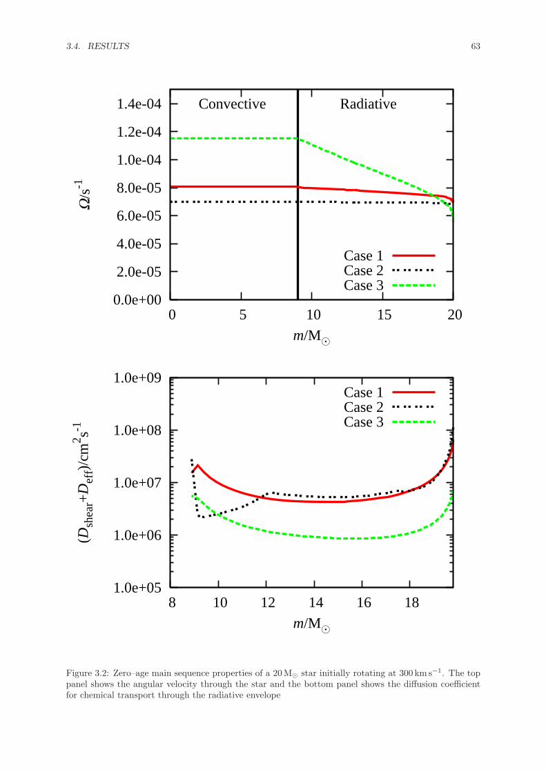
3.4. RESULTS 63
0.0e+00
2.0e-05
4.0e-05
6.0e-05
8.0e-05
1.0e-04
1.2e-04
1.4e-04
0 5 10 15 20
Ω/s
-1
m/M�
Convective Radiative
Case 1Case 2Case 3
1.0e+05
1.0e+06
1.0e+07
1.0e+08
1.0e+09
8 10 12 14 16 18
(Dsh
ear+
Def
f)/c
m2 s-1
m/M�
Case 1Case 2Case 3
Figure 3.2: Zero–age main sequence properties of a 20M� star initially rotating at 300 km s−1. The toppanel shows the angular velocity through the star and the bottom panel shows the diffusion coefficientfor chemical transport through the radiative envelope

64 CHAPTER 3. COMPARISON OF STELLAR ROTATION MODELS
0.0e+00
2.0e-05
4.0e-05
6.0e-05
8.0e-05
1.0e-04
1.2e-04
1.4e-04
1.6e-04
1.8e-04
0 5 10 15 20
Ω/s
-1
m/M�
Conv. Rad. Case 1Case 2Case 3
1.0e+06
1.0e+07
1.0e+08
1.0e+09
1.0e+10
1.0e+11
1.0e+12
1.0e+13
6 8 10 12 14 16 18
(Dsh
ear+
Def
f)/c
m2 s-1
m/M�
Case 1Case 2Case 3
Figure 3.3: Terminal–age main sequence properties of a 20M� star initially rotating at 300 km s−1. Thetop panel shows the angular velocity through the star and the bottom panel shows the diffusion coefficientfor chemical transport through the radiative envelope. The vertical line of the top panel separates theconvective and radiative zones of the case–1 star.

3.4. RESULTS 65
2
2.5
3
3.5
4
4.5
5
5.5
6
6.5
3.6 3.8 4 4.2 4.4 4.6 4.8
log 1
0(L
/L�
)
log10(Teff/K)
5 M�
10 M�
20 M�
50 M�
100 M�
0 km s-1
100 km s-1
200 km s-1
400 km s-1
Figure 3.4: Stellar evolution tracks for stars between 5M� and 100M� calculated with rose for case 1with surface velocities of 0 to 400 km s−1. The tracks for cases 4, 5 and 6, where the angular momentumtransport in convective zones is varied, are almost indistinguishable from each other but produce moreluminous stars than in case 1. There is significant difference between the predictions made for cases 2and 3, where the angular momentum transport in radiative zones is varied.
of the case–3 star rotating faster than in case 1 but is mostly because of the inclusion
of the mean molecular weight gradient in the formulation for case 1. Frischknecht et al.
(2010), who use a model very similar to our case 1, predict a much greater decline in
the mixing near the core but we have been unable to reproduce this. It is likely that the
difference is a result of the inhibiting effect of the mean molecular weight gradient on the
rotational mixing. Whilst it is included in our models, the results of Frischknecht et al.
(2010) suggest that, towards the end of the main–sequence, its effect covers a much larger
proportion of the radiative envelope than in our models.
3.4.2 Effect on Hertzsprung–Russell diagram
As expected, the effects of rotation on the structure and chemical evolution of each star
are significant across the HR diagram. We have plotted the case–1 models in Fig 3.4.
Centrifugal forces cause the star to expand making it dimmer and redder. However,
because of the additional chemical mixing, more hydrogen is made available during the
main sequence so, by the TAMS, rotating stars are generally more luminous than similar
mass non–rotating stars. This effect becomes more pronounced at higher rotation rates

66 CHAPTER 3. COMPARISON OF STELLAR ROTATION MODELS
2
2.5
3
3.5
4
4.5
5
5.5
6
6.5
3.6 3.8 4 4.2 4.4 4.6 4.8
log 1
0(L
/L�
)
log10(Teff/K)
5M�
10M�
20M�
50M�
100M�
Case 1Case 2Case 3
Figure 3.5: Stellar evolution tracks for stars between 5M� and 100M� with initial surface rotationof 300 km s−1 for cases 1, 2 and 3. The model of Heger et al. (2000) predicts a greater enhancementand higher surface temperatures compared to that based on Maeder (2003) for stars more massive than10M�.
and is most apparent for stars with masses up to 20 M�.
There are clear differences between the predicted evolution of rotating stars in each
of the three cases. Fig. 3.5 shows the evolution of five different stellar masses in the HR
diagram for cases 1, 2 and 3 with an initial surface rotation of 300 km s−1. These cases
are the three different models of rotational mixing in radiative zones at solar metallicity.
Rotating case–1 stars appear to be the most luminous at low masses but least luminous
at high masses. Case–2 stars are also consistently cooler than their case–1 and case–3
equivalents except below 10 M�. This is because the strength of rotation–induced mixing
increases rapidly with mass in case–2 stars unlike in cases 1 and 3, where the difference
is more modest.
Although there is apparently a large difference between the three models in the HR
diagram, to distinguish between them from stellar populations requires either a very large
sample or accurate independent measurements of stellar masses and rotation velocities.
Both of these are very challenging but, with the advent of large scale surveys, the former
is quickly becoming a possibility.

3.4. RESULTS 67
3.4.3 Nitrogen enrichment
Currently the key test for any model of stellar rotation is how well it reproduces the spread
of data in a Hunter diagram (Hunter et al., 2009). Hunter plotted nitrogen enrichment
against surface rotation. Large scale surveys, such as the VLT–FLAMES Tarantula sur-
vey (Evans, 2011), will greatly increase the data available for surface rotation velocities
and surface abundances over the coming decade. Thus, if different models can be distin-
guished in a Hunter diagram, this would form a key test for stellar rotation models.
In Fig. 3.6 we plot our theoretical Hunter diagram for 10 M� and 60 M� stars at
different initial surface rotation velocities with the different radiative–zone models at
solar metallicity. Each star begins at the bottom of the plot with the same nitrogen
abundance but different initial surface velocities. There is an initial period where the
star spins down before any enrichment has occurred. During this time the star moves
straight to the left of the plot. Eventually the surface nitrogen abundance begins to
increase because of rotation induced mixing from the burning region. At the same time
the star continues to spin down because of mass loss and structural evolution. The net
effect is that the star moves towards the upper left–hand region of the plot. At the end
of the main sequence the star expands and rapidly spins down. This appears as a near–
horizontal line as the star moves rapidly towards the left–hand edge of the plot. Some
further enrichment may occur during the giant phase.
The evolution of the surface abundances is very model dependent. Case 3, which is
based on the early model of Zahn (1992), gives more nitrogen enrichment than case 1
at high masses (M ≥ 60 M�) but significantly less at low masses (M ≤ 10 M�). Most
notably though, the case–3 stars spin down to a far greater degree before enrichment
occurs. We attribute this to the neglect of mean molecular weight gradients. Mixing
near the core is more efficient in case 3 but, owing to the overall calibration, is weaker
near the surface.
For case 2 the amount of mixing in lower–mass stars is much less than for both cases
1 and 3. By comparison the enrichment of case–2 60 M� stars is greater than in the
other two cases, particularly for slower rotators. This mass dependent behaviour of the
rotating models could provide important clues to distinguish between the models.
At solar metallicity, owing to the enhanced mass loss, massive stars spin down before
the end of the main sequence so, in this case, we would not observe the absence of the
moderately rotating, highly enriched stars seen at low metallicity (Hunter et al., 2009).
Observations of multiple clusters at different ages at this metallicity would be a good test
for rotating stellar models because the evolution across the Hunter diagram is significantly
different in each case even when they are calibrated to give the same level of enrichment
at the end of the main sequence.

68 CHAPTER 3. COMPARISON OF STELLAR ROTATION MODELS
8
8.2
8.4
8.6
8.8
9
9.2
0 50 100 150 200 250 300 350 400 450
12+
log 1
0[N
/H]
v/km s-1
10M�
Case 1Case 2Case 3
8
8.2
8.4
8.6
8.8
9
9.2
9.4
0 50 100 150 200 250 300 350 400
12+
log 1
0[N
/H]
v/km s-1
60M�
Case 1Case 2Case 3
Figure 3.6: Nitrogen enrichment (by number of nuclei) variation with initial surface rotation for cases 1,2 and 3. Stars start on the ZAMS with low nitrogen abundances and high velocities and evolve to higherabundances and lower velocities during the main sequence. The top panel is for 10M� stars and thebottom panel is for 60M� stars. Note the different scales for each panel. As expected the enrichment ismuch greater for more massive stars. Case–3 stars spin down more before any enrichment occurs. Theygive greater enrichment than either of the other two models at high masses but significantly less thancase 1 for low masses. Cases 1 and 2 enrich to a similar degree for the high–mass stars but case 2 exhibitssignificantly less enrichment for low–mass stars than case 1.

3.4. RESULTS 69
3.4.4 Helium–3 enrichment
Apart from the enrichment of nitrogen, rotation can have a large effect on the evolution of
other elements. Changes in the carbon and oxygen abundances in rotating stars predicted
from models have been considered but the accuracy of the data prohibits any strong
conclusions from being made. Frischknecht et al. (2010) discuss the effect rotation may
have on the surface abundances of light elements. We consider here the evolution of the
surface abundance of 3He. A similar analysis could be performed for other elements such
as lithium and boron. The changes in the overall abundance of 3He because of rotation
could partially explain the discrepancy between the predicted abundances produced by
stars and the lack of enrichment of the inter–stellar medium compared to levels predicted
by primordial nucleosynthesis (Dearborn et al., 1986, 1996; Hata et al., 1995). This has
been explained in the past by thermohaline mixing (Stancliffe, 2010) but, as our results
show, the surface 3He abundance is strongly affected by rotation and so it is likely to
make at least some contribution to this effect. We leave the issue of whether the total
production increases or decreases over the stellar lifetime to future work. In either case,
the evolution of helium–3 with respect to the surface rotation is very different between
alternative models and so, as for nitrogen enrichment, this would form a useful comparison
of stellar rotation models. Unlike nitrogen, helium–3 enrichment is stronger at low masses
and so provides a greater number of candidate stars for observations.
Fig. 3.7 shows the helium–3 enrichment for 10 M� and 60 M� stars of varying initial
surface velocities for each of the different radiative zone models at solar metallicity. As
for nitrogen, all three cases show comparable amounts of enrichment in high–mass stars.
The amount of enrichment at the end of the main sequence is the same in each case but
case–3 stars are slightly more enriched at all rotation rates. Case–3 stars spin down much
more before enrichment occurs so the paths for these stars lie to the left of case–1 and
case–2 stars but the amount of enrichment at the end of the main sequence is comparable
to, though slightly higher than, the other two cases.
The difference between the test cases is far greater at lower masses. Both case–2 and
case–3 stars show substantially less enrichment during the main sequence especially for
slow rotators and case–3 stars have much slower surface rotation at the end of the main
sequence than in the other two cases. Both of these contribute to very different evolution
which should be distinguishable observationally. Indeed, whilst the models may produce
similar results for full population synthesis calculations, it has been found that there
is often far less agreement when different mass ranges are considered separately (Brott
et al., 2011a).
3.4.5 Metallicity dependence
In order to compare stellar rotation models with data it is important to distinguish which
effects are observable at different metallicities. Low–metallicity stars are particularly

70 CHAPTER 3. COMPARISON OF STELLAR ROTATION MODELS
2
3
4
5
6
7
8
0 50 100 150 200 250 300 350 400 450
12+
log 1
0[3 H
e/H
]
v/km s-1
10M�
Case 1Case 2Case 3
2 2.5
3 3.5
4 4.5
5 5.5
6 6.5
0 50 100 150 200 250 300 350 400
12+
log 1
0[3 H
e/H
]
v/km s-1
60M�
Case 1Case 2Case 3
Figure 3.7: Helium–3 enrichment variation with initial surface rotation for cases 1, 2 and 3. The toppanel is for 10M� stars and the bottom panel is for 60M� stars. At high masses all three cases showa similar degree of TAMS enrichment though there is some variation in the evolutionary paths in eachcase. Case–3 stars spin down more before enrichment occurs and so lie to the left of the other two cases.At low masses, both case–2 and case–3 stars are less enriched at the TAMS than case–1 stars. This isespecially true for slow rotators.

3.4. RESULTS 71
useful because they have significantly lower mass–loss rates (Vink et al., 2001). For stars
of metallicity Z = 0.001 the mass–loss rate is roughly ten times lower than at solar
metallicity. This allows us to rule out effects on the models produced by our prescription
for mass loss.
The low–metallicity cases show similar distinctions in the HR diagram to those at
solar metallicity, although high–mass, rapidly rotating, case–2 stars are sufficiently well
mixed to undergo quasi–homogeneous evolution. There are also significant differences
in the nitrogen enrichment between the different models. Because the mass–loss rate
is lower in low–metallicity stars they retain their surface rotation for much longer so
the main sequence appears much more vertical in a Hunter diagram. Unlike the solar
metallicity cases, case 2Z exhibits significantly more mixing than case 1Z particularly for
slow and moderately rotating stars (Fig. 3.8). This is the complete opposite of the results
at solar metallicity and highlights the importance of testing different stellar environments
to discover clues to distinguish between different models. In contrast, the enrichment of
helium–3 in case 2Z stars is less than in case 1Z .
3.4.6 Surface gravity cut–off
As a consequence of increasing stellar radius and angular momentum conservation all
models for stellar rotation predict a rapid decay in the surface rotation velocity after
the end of the main sequence. Observations suggest that, even for rotating stars, there
is a sharp cut–off in the effective gravity at log10(g/cm2s−1) ≈ 3.2 when a star leaves
the main sequence and moves over to the giant branch (Brott et al., 2011b). This effect
depends on stars reaching the TAMS without spinning down too much during the main
sequence. Therefore it is more easily seen at lower metallicities where the mass–loss rate
is lower. The observed value for the TAMS gravity can be enforced in rotating models
by including a degree of overshooting. However this simply introduces an additional free
parameter into the models. In Fig. 3.9 we show the different cut–offs in the effective
gravity predicted by cases 1Z , 2Z and 3Z . The end of the main sequence is indicated by
a distinct cusp in the path of the star in the range 3 < log10(g/cm2s−1) < 4. Note that
the expected number of stars with significant rotation after the main–sequence cut–off is
low because the evolution to a very slowly rotating giant is extremely rapid compared to
the rest of the main sequence.
For higher–mass stars there is a sharp cut–off in the surface gravity at the end of
the main sequence that is the same regardless of the model used although the TAMS
surface rotation is somewhat higher in case 2. The mixing in low–metallicity, high–mass,
rapidly rotating, case–2 stars is very efficient and so they evolve almost homogeneously
and thus they appear differently in the plot. For lower–mass stars the change in surface
gravity at the end of the main sequence is still clear but varies by around an order of
magnitude across all rotation rates and test cases. Case–2 and case–3 stars have lower
terminal–age main–sequence surface gravities than case–1 stars and show a tendency

72 CHAPTER 3. COMPARISON OF STELLAR ROTATION MODELS
4
4.5
5
5.5
6
6.5
7
7.5
8
0 100 200 300 400 500
12+
log 1
0[3 H
e/H
]
v/km s-1
10M�
Case 1Z
Case 2Z
Case 3Z
7
7.5
8
8.5
0 100 200 300 400 500 600
12+
Log
[N/H
]
v/kms-1
60M�
Case 1Z
Case 2Z
Case 3Z
Figure 3.8: Chemical enrichment variation at low metallicity. The top panel shows the enrichment ofhelium–3 and the bottom panel shows the enrichment of nitrogen. The upper plot is for 10M� stars andthe lower plot is for 60M� stars. Case 2Z now shows much higher nitrogen enrichment than case 1Z , theopposite to what we found in the solar metallicity cases. The enrichment of helium–3 in case 2Z stars isstill considerably less than in case 1Z .

3.4. RESULTS 73
0
100
200
300
400
500
2.5 3 3.5 4 4.5
v/km
s-1
log10(geff/cm s-2)
10M�
Case 1Z
Case 2Z
Case 3Z
0
50
100
150
200
250
300
350
400
2.5 3 3.5 4 4.5
v/km
s-1
log10(geff/cm s-2)
60M�
Case 1Z
Case 2Z
Case 3Z
Figure 3.9: The effective gravity variation with surface velocity for 10M� stars (top panel) and 60M�stars (bottom panel) for cases 1Z , 2Z and 3Z . The end of the main sequence occurs at the right–mostcusp of each path. Although the surface gravity is similar for all the models and all initial rotation rates,the TAMS surface velocities are very different between the different cases. Exceptions to this are therapidly–rotating, high–mass, case–2Z stars which undergo almost homogeneous evolution.

74 CHAPTER 3. COMPARISON OF STELLAR ROTATION MODELS
towards lower TAMS surface gravities for more rapid rotators. Case–3 stars generally have
lower rotation rates at the end of the main sequence for low–mass stars. This distinguishes
them from case 2. Once again we see that the difference in stellar properties predicted
by each model is strongly dependent on rotation rate, mass and metallicity suggesting
that it is essential to explore populations covering as wide a range as possible in order to
test rotating models.
3.4.7 Alternative models for convection
In order to compare the difference in the evolution of a star owing to the details of the
model for convective angular momentum transport we now focus on cases 1, 4, 5 and
6. Uniform specific angular momentum in the core causes more shear mixing near the
core–envelope boundary than when the core is solid body rotating as shown in Fig. 3.10.
This results in higher luminosity stars with similar temperatures. There is almost no
difference between cases 4, 5 and 6 in the HR diagram.
When we compare the different models for convection in a Hunter diagram we see
that cases 4, 5 and 6, which have uniform specific angular momentum throughout their
convective zones, have significantly more enrichment for all masses and rotation rates
than case 1. The difference is more pronounced for higher–mass rapid rotators (Fig. 3.11).
However, we note that it is more difficult to distinguish between cases 4, 5 and 6. For the
highest mass stars we do find some difference in the enrichment of nitrogen and helium–3
between the models but recall that there is a difference in Dcon of four orders of magnitude
between cases 5 and 6.
Given the small magnitude of the change in enrichment and structure over such a
range of diffusion coefficients it seems unlikely that these tests can adequately distinguish
between convective models. In addition, adjusting the calibration of case 1 could produce
a very similar effect making it difficult even to distinguish between n = 0 and n = 2 models
from observations. At the same time though, it is interesting to note the significant change
that modifying the core angular momentum distribution has had on the evolution of the
surface composition.
3.5 Conclusions
Rotation in stars has a number of profound effects on their evolution. Not only are there
significant changes in the hydrostatic structure (Endal and Sofia, 1978) but this causes a
thermal imbalance that can lead to a strong meridional circulation current (Sweet, 1950).
Meridional circulation leads to additional shear which induces a number of instabilities.
The resulting turbulence leads to strong mixing of both angular momentum and chemical
composition.
Although most modellers include all of these effects, the exact implementation of
stellar rotation can vary dramatically. For example Heger et al. (2000) use a model

3.5. CONCLUSIONS 75
0.0e+00
1.0e-04
2.0e-04
3.0e-04
4.0e-04
5.0e-04
0 10 20 30 40 50 60
Ω/s
-1
m/M�
Conv. Rad.
Case 1Case 4Case 5Case 6
0.0e+00
1.0e-04
2.0e-04
3.0e-04
4.0e-04
5.0e-04
0 10 20 30 40 50
Ω/s
-1
m/M�
Conv. Rad.
Case 1Case 4Case 5Case 6
Figure 3.10: Angular velocity distributions for 60M� stars initially rotating at 300 km s−1 for differentconvective models. The top panel shows the ZAMS distributions and the bottom panel shows the TAMSdistributions. Despite there being four orders of magnitude difference between the convective diffusioncoefficients in cases 4, 5 and 6, there is very little difference between the angular velocity distributionsthey predict. In each case, the models with uniform specific angular momentum in convective zonespredict more shear at the convective boundary than the models with solid body rotation in convectivezones.

76 CHAPTER 3. COMPARISON OF STELLAR ROTATION MODELS
8
8.2
8.4
8.6
8.8
9
9.2
0 50 100 150 200 250 300 350 400 450
12+
Log
[N/H
]
v/kms-1
10M�
Case 1Case 4Case 5Case 6
8
8.5
9
9.5
10
0 50 100 150 200 250 300 350 400 450
12+
Log
[N/H
]
v/kms-1
60M�
Case 1Case 4Case 5Case 6
Figure 3.11: Nitrogen enrichment variation with initial surface rotation for cases 4, 5 and 6. The toppanel is for 10M� stars and the bottom panel is for 60M� stars. As expected the enrichment is muchgreater for more massive stars. There is much more enrichment for models in which the core has uniformspecific angular momentum, an effect that becomes progressively more pronounced for higher massesand rotation rates
.

3.5. CONCLUSIONS 77
where meridional circulation is treated diffusively. The diffusion owing to shear is the
linear combination of a number of coefficients based on different possible instabilities.
On the other hand, modellers such as Zahn (1992), Talon et al. (1997) and Maeder
(2003) treat the circulation as advective and use a single diffusion coefficient based on
the magnitude of Kelvin–Helmholtz instabilities induced by shear. In these models it
is also necessary to define the magnitude of diffusion along isobars and this too varies
between different models.
We have shown that different models generally give rise to similar qualitative con-
clusions but there are significant differences in the results based on mass, rotation rate
and metallicity. There are also open questions about how angular momentum transport
occurs in convective zones.
Comparing the models based on Talon et al. (1997) and Maeder (2003), case 1, and
that based on Heger et al. (2000), case 2, we find that case 1 gives higher luminosity stars
for masses less massive than 10 M� and more luminous, hotter stars at higher masses than
case 2. High–mass stars give similar levels of nitrogen enrichment in each case but case 2
produces far less enrichment for low–mass and intermediate–mass stars than case 1. The
situation is similar for their helium–3 enrichment.
The predicted effects of rotation appear to be highly dependent on the metallicity.
This is one of the clearest tests for different stellar rotation models. At metallicity of
Z = 0.001, case 2 actually produces significantly more nitrogen enrichment in high–mass
stars although the degree of helium–3 enrichment is still lower in case 2 than case 1.
Additional effects such as the variation of the surface gravity with respect to surface
rotation velocity are seen in lower–metallicity stars where the mass–loss rate is lower.
We see a sharp cut–off in the effective gravity at the end of the main sequence but the
TAMS rotation rates are very different between different models. Case–2 stars reach the
end of the main sequence with higher rotation rates than the other two cases for both
low–and high–mass stars. Case–1 stars reach the end of the main sequence with higher
surface gravity than the other two cases but only for lower–mass stars.
All current models treat convective zones as rotating solid bodies. This may be justified
if convective zones can generate sufficiently strong magnetic fields (e.g. Spruit, 1999) but,
if not, hydrodynamic models and calculations suggest that convective zones should tend
towards uniform specific angular momentum (Lesaffre et al., in prep., Arnett and Meakin,
2010). Identifying whether this is the case or not is difficult from surface observations.
There is no significant change in the paths of stars across the HR diagram between cases 4,
5 and 6. In fact, there is no test we have found that would adequately differentiate between
these three cases even though the diffusion coefficient in convective zones varies by four
orders of magnitude. There are some minor differences in the amount of enrichment for
massive stars but these would be hard to test with existing data. The models with uniform
specific angular momentum generally produce slightly more luminous stars and higher
surface chemical enrichment than those models with solidly rotating cores. However,

78 CHAPTER 3. COMPARISON OF STELLAR ROTATION MODELS
slightly less efficient mixing in the radiative zone could mask this difference.
We have thus far not included magnetic fields in the models. It has been suggested
that the strong turbulence generated by rotation could result in a radiative magnetic
dynamo (Spruit, 1999). A sufficiently strong magnetic field can effectively suppress the
meridional circulation and reduce the overall shear (Maeder and Meynet, 2005). It could
also result in additional mass and angular momentum loss (e.g. Lau et al., 2011; ud-Doula
and Owocki, 2002). As with rotation, there is little consensus on the details of magnetic
field generation but it is generally accepted that the effects of rotation and magnetic fields
cannot be considered in isolation. In chapter 5 we include magnetic fields in rose in a
similar manner in order to better explore this important feature of stellar evolution.
Owing to the range of available models, it is an extremely challenging problem to try to
identify the one which best fits observed stellar populations. Now that large scale surveys
are starting to produce data for many stars in different regions it is becoming possible to
make progress and isolate which effects dominate. The key to distinguishing the relevant
physics seems to be taking measurements of groups of stars at different masses, ages
and metallicities. In individual clusters, models should be able to match not only the
full distribution of observed stars but also the expected distribution in each mass range.
Whilst most of the models can be calibrated to fit the data for a single cluster, we have
shown that the behaviour of each model is highly dependent on mass and metallicity and
so being able to fit data for a range of stellar environments is the true test of any model.

79
A few observation and much reasoning lead to
error; many observations and a little reasoning
to truth. (Alexis Carrel)
4Model–dependent characteristics of stellar populations
4.1 Introduction
The effect of rotation on the internal physics of stars has been considered for many years
(e.g. Kippenhahn et al., 1970). Rotation causes significant changes in the hydrostatic
balance of the star (Endal and Sofia, 1978), thermal imbalance causes a meridional cir-
culation current (Sweet, 1950) and differential rotation leads to shear instabilities (e.g.
Spiegel and Zahn, 1970). These all result in mixing of angular momentum and chemical el-
ements within the star leading to changes its surface properties such as the surface gravity,
temperature, luminosity and chemical composition. Over the course of several decades,
the physical formulations used to describe stellar rotation have proliferated (Heger et al.,
2000; Maeder and Meynet, 2005; Meynet and Maeder, 1997; Talon et al., 1997; Zahn,
1992). Whilst each new model has been suitably justified physically, there has been lit-
tle observational data to back up claims of improved physical agreement. This leads to
the possibility that any number of physical models can be chosen to produce a range of
desired results which may or may not be accurate. This situation is worsened because
the data required to constrain the models is scarce. However, with the observations of
the VLT–FLAMES survey of massive stars (Evans et al., 2005, 2006) and VLT–FLAMES
Tarantula survey (Evans, 2011) it is now becoming possible to make such comparisons of
different physical models and place some constraints on the formulations used.
Comparing stellar models is still problematic because of the difficulty of isolating
the effects of rotation from other physical and numerical differences in the results of
other groups. In chapter 3 we presented rose, a code capable of performing stellar
evolution calculations with a number of different models of stellar rotation, eliminating

80 CHAPTER 4. MODEL–DEPENDENT CHARACTERISTICS OF STELLAR POPULATIONS
any differences owing to other numerical or physical effects between different codes.
In chapter 3 we considered the main differences between the evolution of individual
stars under the assumptions of several popular models. In this chapter we combine that
analysis with the stellar population code, starmaker (Brott et al., 2011a), to determine
the differences in stellar populations that arise from two physical models. One is based
upon Heger et al. (2000) and has solely diffusive transport of angular momentum. The
other is based on Talon et al. (1997) and Maeder (2003) and has both diffusive and
advective transport of angular momentum. The two different models have very different
diffusion coefficients and there are marked differences in the results for individual stars.
It is possible to get better agreement between the models under different criteria by
adjusting the associated unknown constants but this leads to poorer agreement elsewhere.
One particular consequence of different input physics that we found in chapter 3 is that
the mass dependence of the mixing is very different in each case. The models agree in
that the total enrichment in low–mass stars (M < 20 M�) is much less than in high–mass
stars (M > 20 M�). However, the enrichment found with each model is very different for
low–mass stars despite reasonable agreement for high–mass stars. In chapter 3 we also
concluded that the difference between the two models varies for different metallicities. For
Z = 0.001, the model based on Heger et al. (2000) actually produces significantly more
nitrogen enrichment in high–mass stars, particularly for slow and moderate rotators. We
shall explore all of these features further in this chapter.
In section 4.2 we briefly review the physics of the models. For full descriptions we
refer the reader to chapter 2 and Brott et al. (2011b). We also describe the models under
comparison. In section 4.3 we compare the stellar population predictions and consider
the similarities and differences between the models and in section 4.4 we present our
summary and conclusions.
4.2 Input physics
Each grid of models is produced with the code rose described in section 2.3.6. The
physical model for the evolution of rotating stars is described in section 2.3. The stellar
populations are then generated with the code starmaker (Brott et al., 2011b), described
in section 2.5. It was originally designed to work with the evolutionary models of Brott
et al. (2011a). We have adapted it for use with rose stellar evolution models. Based
on a grid of evolutionary models, starmaker interpolates for stellar properties given
an initial mass, initial surface velocity and age. These are chosen at random according
to user–defined distribution functions. Each simulated star is assigned a random orien-
tation in space. The newly generated sample can subsequently be filtered according to
observational selection effects to enable comparison with observed samples.
In this chapter we consider two models for comparison, these are case 1 and case 2
from chapter 3. For both models we evolve a grid of stars with masses between 3 M� and

4.2. INPUT PHYSICS 81
100 M� and initial equatorial surface rotation velocities between 0 and 600 km s−1. The
zero age main sequence is taken to be the point of minimum luminosity at the onset of
hydrogen burning. The masses computed are
m/M� ∈{3, 4, 5, 6, 7, 8, 9, 10, 12, 15, 20, 25,
30, 35, 40, 45, 50, 55, 60, 65, 70, 75, 80,
85, 90, 95, 100} (4.1)
and for each mass the initial surface velocities used are
vini/km s−1 ∈{0, 50, 100, 150, 200, 250, 300,
350, 400, 450, 500, 550, 600}, (4.2)
except when the rotation velocity would be too close to critical rotation to achieve nu-
merical convergence. This becomes more difficult for stars less massive than 10 M�.
Convergence can be achieved for a 10 M� star rotating faster than 95% of critical rota-
tion, although the assumptions of the model are likely to become invalid this close to
critical. For a 3 M� star the limit for convergence is close to 70% of critical rotation.
Both the case 1 and case 2 models for each mass and initial surface velocity must reach
the end of the main sequence for either of them to be used in the grid. The end of the
main sequence is taken as the point of maximum temperature before a star moves onto
the Hertzsprung gap. Each model evolved is plotted in Fig. 4.1. For both models, the
diffusion of angular momentum in convective zones is determined by the characteristic
eddy viscosity given by mixing length theory such that Dconv = Dmlt = 13vmltlmlt. The
position of the convective boundary is determined by the Schwarzschild criterion and
although the code includes a model for convective overshooting, we do not use it in these
simulations. Unlike for chapter 3, we only consider the case in which the convective core
tends to a state of solid body rotation. In section 4.3.5 we examine the effects of changing
the free parameters associated with the model. Models generated with this calibration
are referred to as case 2b. In this chapter we generate models with two different metal-
licities, Galactic and LMC, as defined by Brott et al. (2011a). Other than the initial
composition, the input physics is the same for both metallicities. However, for clarity, we
distinguish models that use LMC metallicity by referring to them with a superscript ‘Z’
(e.g. case 1Z).
The angular momentum evolves according to
∂(r2Ω)
∂t=
1
5ρr2
∂(ρr4ΩU)
∂r+
1
ρr2
∂
∂r
(ρDKHr4 ∂Ω
∂r
)+
1
ρr2
∂
∂r
(ρDconr
2 ∂Ω
∂r
). (4.3)

82 CHAPTER 4. MODEL–DEPENDENT CHARACTERISTICS OF STELLAR POPULATIONS
0
100
200
300
400
500
600
0 10 20 30 40 50 60 70 80 90 100
v/km
s-1
M/MO•
0
100
200
300
400
500
600
0 10 20 30 40 50 60 70 80 90 100
v/km
s-1
M/MO•
Figure 4.1: Grid of initial models, in initial mass–initial equatorial velocity space, used for simulatingstellar populations.
This is equation (2.24) with n = 2. The terms are described in more detail in chapter 2.
The primary difference between the cases is the treatment of meridional circulation U
and the diffusion coefficient DKH.
4.2.1 Case 1
Our case 1 model uses the formulation for DKH of Talon et al. (1997),
DKH = C0
2Ric(r dΩ
dr
)2N2
T /(K + Dh) + N2μ/Dh
, (4.4)
where
N2T = − geff
HP
(∂ ln ρ
∂ ln T
)P,μ
(∇ad −∇) (4.5)
and
N2μ =
geff
HP
(∂ ln ρ
∂ ln μ
)P,T
d ln μ
d ln P. (4.6)
As in chapter 3 we follow Maeder (2003) by taking the critical Richardson number,
Ric = (0.8836)2/2. We have also chosen C0 so that we reproduce the terminal–age main–

4.2. INPUT PHYSICS 83
Age/yr Number of Maximum mass Maximum massstars remaining (case 1)/M� (case 2)/M�
5 × 10⁶ 9749375 42.2 41.6107 9168582 21.6 22.3
2 × 10⁷ 8318064 14.1 13.75 × 10⁷ 6449586 8.2 7.4
Table 4.1: The properties of different single–aged stellar populations used in section 4.3. The originalsize of the population in each case is 107 stars. Each population is generated by an instantaneous burstof star formation at t = 0. The first column shows the age of the simulated population. The secondcolumn shows the number of stars remaining in the sample after stars that have reached the end of themain sequence are excluded. The third and fourth columns show the mass of the most massive starremaining in the sample at the given age for case 1 and case 2 respectively.
sequence (TAMS) nitrogen enrichment of a 40 M� star initially rotating at 270 km s−1 with
Galactic composition given by Brott et al. (2011b). The effective diffusion coefficient Deff
is
Deff =|rU |230Dh
(4.7)
and we take
Dh = 0.134r (rΩV (2V − αU))13 , (4.8)
where
α =1
2
d(r2Ω)
dr. (4.9)
4.2.2 Case 2
Our case 2 model is that of Heger et al. (2000). In this case U = 0 because circulation is
treated as a purely diffusive process. The details of the various diffusion coefficients are
extensive so we refer the reader to the original paper. With their notation the diffusion
coefficients are
DKH = Dsem + DDSI + DSHI + DSSI + DES + DGSF (4.10)
and
Deff = (fc − 1)(DDSI + DSHI + DSSI + DES + DGSF), (4.11)
where each Di corresponds to a different hydrodynamic instability. Heger et al. (2000)
take fc = 1/30 and we use this too. We also use fμ = 0. The consequences of this
are discussed in chapter 3. Unless otherwise stated, we calibrate this model by scaling
DES, the dominant diffusion coefficient, so that the nitrogen enrichment of a 20 M�, solar
metallicity star with initial surface angular velocity of 300 km s−1 is the same as for case 1
at the TAMS.

84 CHAPTER 4. MODEL–DEPENDENT CHARACTERISTICS OF STELLAR POPULATIONS
4.2.3 Stellar populations
Throughout this paper we use a variety of populations at different ages with different
star formation histories. The main reason for this is that, as a population ages, the mass
of the most massive stars remaining in the main–sequence population decreases, whilst
stars much less massive than the maximum mass have not had sufficient time to produce
significant nitrogen enrichment. The combination of these tendencies allows us to follow
how the amount of enrichment varies with mass. This applies specifically to clusters in
which we expect the range of ages of the stars to be small compared to the age of the
cluster. It is important to note that rotation can significantly affect the upper bound
to the mass of stars in the population. The populations used in this paper are listed in
Table 4.2.3. For the figures in section 4.3 we compare the data using 2D histograms for
which we have separated the data into a grid of 50 × 50 bins. The number of stars in
each bin divided by the total number of stars. In case 1 this is n1 and similarly n2 for
case 2. In each comparison we reduce the size of the larger population to be the same
size as the other by randomly removing stars.
4.3 Results
We simulated stellar populations at a number of ages and metallicities for each model
and found a number of significant differences.
4.3.1 The Hertzsprung–Russell diagram
When we look at the effect of the two models of rotation on stars in the Hertzsprung–
Russell (HR) diagram we find that there is very little difference between them. Whilst
there is variation in the TAMS temperatures and luminosities of the stars in each case, the
difference is small and, for a single burst of star formation, only affects a handful of stars
in the population at any given time. For most of a star’s lifetime the predicted position
in the HR diagram is sufficiently similar between the two cases that the difference in the
population cannot be distinguished. Fig. 4.2 shows the HR diagrams for cases 1 and 2
for simulated clusters with an age of 2 × 10⁷ yr. Apart from slightly different degrees of
broadening at the main–sequence turn off, there is no difference between the two cases.
This is true at all ages and if we simulate a population of stars with continuous star
formation we still find only slight distinctions between the two cases. To distinguish
these differences in real stellar populations would be made even more difficult because
the broadening of the high–luminosity end of the main sequence in the HR diagram
owing to rotation is similar to the effect of including binary stars (Eldridge et al., 2008).
This doesn’t mean that mass determinations of rotating stars from their surface rotation,
temperatures and luminosities are unaffected by the specific physics of the model. For
individual models, the difference can be significant but the cumulative effect has little

4.3. RESULTS 85
Case 1
log10(Teff/K)
log 1
0(L
/L�)
4.154.24.254.34.354.44.452
2.5
3
3.5
4
4.5
5
log 1
0(n
1)
−6
−5
−4
−3
−2
Case 2
log10(Teff/K)
log 1
0(L
/L�)
4.154.24.254.34.354.44.452
2.5
3
3.5
4
4.5
5
log 1
0(n
2)
−6
−5
−4
−3
−2
Difference
log10(Teff/K)
log 1
0(L
/L�)
4.154.24.254.34.354.44.452
2.5
3
3.5
4
4.5
5
2|n
1−n2|
n1+
n2+
10−6
0.1
0.2
0.3
0.4
0.5
0.6
0.7
0.8
0.9
Figure 4.2: Hertzsprung–Russell diagrams for a population of stars at age 2×10⁷ yr. There is some slightvariation between the two cases at the end of the main sequence (highest luminosity) but the effect issmall. Otherwise there is no obvious difference between the results produced in cases 1 and 2. Whencomparing the two populations, the addition of 10−6 in the denominator is to avoid division by zero inunpopulated bins.

86 CHAPTER 4. MODEL–DEPENDENT CHARACTERISTICS OF STELLAR POPULATIONS
impact on the population as a whole. It is also important to note that the maximum
mass of stars remaining in the sample varies between the cases because the main–sequence
lifetimes are different. This means that care must be taken when identifying a cluster’s
age with respect to its most massive members if the cluster contains rapid rotators.
4.3.2 Velocity distribution evolution
Because of variations in the amount of mixing and the evolutionary timescale between
the two cases, we might expect differences between the distribution of rotation rates as
the populations evolve. In Fig. 4.3 we plot the velocity distribution of the remaining stars
in the single–aged populations at 2× 10⁷ yr. This is the typical shape of the distribution
at all ages considered and we see that there is very little difference between the two cases.
4.3.3 The Hunter diagram
The surface abundance of various isotopes is an extremely important tracer of the effects
of rotation. In section 4.3.2 we showed that, using alternate models of rotation, we find
only small effects on the velocity distribution in stellar populations. We now consider the
effect of rotation on the surface abundance of nitrogen. We could make similar conclusions
about other chemical elements but their usefulness depends on the accuracy to which they
can be measured and the availability of data. For example in chapter 3 we discussed the
effect of rotation on the surface abundance of helium–3 but this is difficult to measure
and so is not particularly useful in this discussion. Frischknecht et al. (2010) and Brott
et al. (2011b) also consider how rotation is likely to affect the surface abundances of
light elements. If we look at a plot of the surface abundance against surface rotation
rate, commonly referred to as the Hunter diagram (Hunter et al., 2009), for different
ages (Fig. 4.4) we see that there are some very clear differences between the two cases.
At each age, the most massive stars remaining in the population dominate the enriched
stars. Stars more massive than this have already evolved off the main sequence. The
less massive stars in the population evolve more slowly and so have not had enough time
to become enriched. At early times the populations are very similar except that case 1
predicts rather more enrichment for stars rotating slower than 200 km s−1 while case 2
predicts more enrichment of the most rapidly rotating stars. As the population ages, the
amount of enrichment in case 1 stays roughly the same but the amount of enrichment
in case 2 drops off slowly followed by a large drop between 2 × 10⁷ yr and 5 × 10⁷ yr. It
is here, where only stars less massive than 8.2 M� remain, that the difference between
the models is clearest. However, even at 2 × 10⁷ yr, we can see that there are far more
enriched stars in case 1 than case 2 compared with earlier times.
If we consider the case–dependence of the Hunter diagrams for a population of stars
with a continuous star formation history we find much the same thing. Fig. 4.5 shows
that, although both cases follow a trend of more frequent enrichment in stars with higher

4.3. RESULTS 87
0 100 200 300 400 500 6000
0.5
1
1.5
2
2.5
3
3.5
4
4.5
5x 10
−3 Case 1
v/km s–1
n1
0 100 200 300 400 500 6000
0.5
1
1.5
2
2.5
3
3.5
4
4.5
5x 10
−3 Case 2
v/km s–1
n2
Figure 4.3: Velocity distribution of stars in cases 1 and 2 both at an age of 2×10⁷ yr for the populationsdescribed in table 4.2.3. For this and subsequent figures, v is the projected surface rotation velocity.There is no marked difference between the two distributions.

88 CHAPTER 4. MODEL–DEPENDENT CHARACTERISTICS OF STELLAR POPULATIONS
Case 1
v/kms–1
12+
log 1
0[N
/H]
100 200 300 400 500
7.8
8
8.2
8.4
8.6
8.8
9
9.2
9.4
log 1
0(n
1)
−6.5
−6
−5.5
−5
−4.5
−4
−3.5
−3
−2.5
−2
−1.5
Case 2
v/kms–112
+lo
g 10[N
/H]
100 200 300 400 500
7.8
8
8.2
8.4
8.6
8.8
9
9.2
9.4
log 1
0(n
2)
−6.5
−6
−5.5
−5
−4.5
−4
−3.5
−3
−2.5
−2
−1.5
Difference
v/kms–1
12+
log 1
0[N
/H]
100 200 300 400 500
7.8
8
8.2
8.4
8.6
8.8
9
9.2
9.4
2|n
1−
n2|
n1
+n
2+
10−
6
0.1
0.2
0.3
0.4
0.5
0.6
0.7
0.8
0.9
Case 1
v/kms–1
12+
log 1
0[N
/H]
0 200 400 600
7.8
8
8.2
8.4
8.6
8.8
log 1
0(n
1)
−6.5
−6
−5.5
−5
−4.5
−4
−3.5
−3
−2.5
−2
−1.5
Case 2
v/kms–1
12+
log 1
0[N
/H]
0 200 400 600
7.8
8
8.2
8.4
8.6
8.8
log 1
0(n
2)
−6.5
−6
−5.5
−5
−4.5
−4
−3.5
−3
−2.5
−2
−1.5
Difference
v/kms–1
12+
log 1
0[N
/H]
0 200 400 600
7.8
8
8.2
8.4
8.6
8.8
2|n
1−
n2|
n1
+n
2+
10−
6
0.1
0.2
0.3
0.4
0.5
0.6
0.7
0.8
0.9
Case 1
v/kms–1
12+
log 1
0[N
/H]
0 100 200 300 400 500
7.8
8
8.2
8.4
8.6
8.8
log 1
0(n
1)
−6.5
−6
−5.5
−5
−4.5
−4
−3.5
−3
−2.5
−2
−1.5
Case 2
v/kms–1
12+
log 1
0[N
/H]
0 100 200 300 400 500
7.8
8
8.2
8.4
8.6
8.8
log 1
0(n
2)
−6.5
−6
−5.5
−5
−4.5
−4
−3.5
−3
−2.5
−2
−1.5
Difference
v/kms–1
12+
log 1
0[N
/H]
0 100 200 300 400 500
7.8
8
8.2
8.4
8.6
8.8
2|n
1−
n2|
n1
+n
2+
10−
6
0.1
0.2
0.3
0.4
0.5
0.6
0.7
0.8
0.9
Case 1
v/kms–1
12+
log 1
0[N
/H]
100 200 300 400
7.7
7.8
7.9
8
8.1
8.2
8.3
8.4
8.5
8.6
8.7
log 1
0(n
1)
−6.5
−6
−5.5
−5
−4.5
−4
−3.5
−3
−2.5
−2
Case 2
v/kms–1
12+
log 1
0[N
/H]
100 200 300 400
7.7
7.8
7.9
8
8.1
8.2
8.3
8.4
8.5
8.6
8.7
log 1
0(n
2)
−6.5
−6
−5.5
−5
−4.5
−4
−3.5
−3
−2.5
−2
−1.5
Difference
v/kms–1
12+
log 1
0[N
/H]
100 200 300 400
7.7
7.8
7.9
8
8.1
8.2
8.3
8.4
8.5
8.6
8.7
2|n
1−
n2|
n1
+n
2+
10−
6
0.1
0.2
0.3
0.4
0.5
0.6
0.7
0.8
0.9
Figure 4.4: Hunter diagrams for single–aged populations of stars. From top to bottom, the four rows offigures correspond to 5×10⁶ yr, 107 yr, 2×10⁷ yr and 5×10⁷ yr. At early times the two cases are similarwith slightly more enrichment of the fastest rotators in case 2 and more enrichment of stars rotatingmore slowly than 200 km s−1 in case 1. By 2 × 10⁷ yr we see many more enriched stars in case 1 andby 5 × 10⁷ yr the amount of mixing in case 2 has dropped off dramatically. The jagged right hand edgeof the populations is a result of the grid geometry and the mass–independence of the initial rotationvelocity distribution. Neither affects the large difference we see in the populations at late times.

4.3. RESULTS 89
rotation rates, case 1 produces far more enriched stars than case 2. This is not surprising
because we found far less mixing in case–2 stars at lower masses than in case 1 and it
is these stars that dominate the population. We could have instead chosen to calibrate
case 2 so that there were more mixing in low–mass stars but this would inevitably lead
to a worse match in the populations elsewhere, perhaps in the enrichment of rapidly
rotating very massive stars (M > 40 M�). We discuss this further in section 4.3.5. Also
important to consider is the effect of metallicity. In chapter 3 we found a reversal in the
trend of less mixing in case–2, low–mass stars (M < 20 M�). Increasing the mixing here
to bring the two populations in line would make the low–metallicity agreement far worse.
We discuss this in section 4.3.6.
4.3.4 Effective surface gravity and enrichment
As we suggested in chapter 3, the difference between the two cases can be seen most
clearly by considering different masses of stars. In our discussion of the Hunter diagram
we have appealed to the single–aged population of stars to differentiate between stellar
masses as the population ages. Unfortunately, determining the mass of rotating stars self–
consistently is difficult because of the degeneracy that arises owing to rotation. Fig. 4.6
shows the typical relationship between mass and effective surface gravity in a simulated
population. There is a strong correlation between the two but rotation causes degeneracy
so estimates of the mass from effective gravity alone could be wrong by up to 7 M� in
this case. The correlation does not persist in the case of continuous star formation. Use
of the effective surface gravity is also advantageous because it can be directly determined
spectroscopically. However, caution is necessary for rapid rotators because the effective
gravity is not uniform across the stellar surface (Von Zeipel, 1924). The Hunter diagram
suffers from the problem that, even for simple stellar populations like this one, stars exist
in all regions of the diagram and the population has few clear boundaries. If we look at
the variation of effective surface gravity with nitrogen enrichment the difference between
the models becomes very clear (Fig. 4.7). There are sharp curves that bound the upper
and lower effective surface gravities of the population. The lower bound occurs because
stars evolve rapidly into giants with much lower surface gravity after this limit. The upper
bound occurs because younger stars with higher surface gravities haven’t evolved to the
point where their surface nitrogen is enriched. There are features which distinguish the
two populations at each age. For young populations (5×10⁶ yr) case 2 has a higher upper
bound for nitrogen enrichment and there is a much broader range of surface gravities than
in case 1. For older populations (107 yr and 2 × 10⁷ yr) case 2 predicts generally lower
values for the surface gravity. Finally for old populations (5 × 10⁷ yr) the difference
becomes very stark. The amount of mixing in case 2 drops off dramatically compared to
case 1 while we still predict much lower values for the surface gravity in rapid rotators.
When we consider a population of stars with continuous star formation history, the
difference in the populations is still clear. Interestingly, unlike the Hunter diagram,

90 CHAPTER 4. MODEL–DEPENDENT CHARACTERISTICS OF STELLAR POPULATIONS
Case 1
v/km s–1
12+
log 1
0[N
/H]
0 100 200 300 400 500
7.8
8
8.2
8.4
8.6
8.8
9
log 1
0(n
1)
−7
−6
−5
−4
−3
−2
Case 2
v/km s–1
12+
log 1
0[N
/H]
0 100 200 300 400 500
7.8
8
8.2
8.4
8.6
8.8
9
log 1
0(n
2)
−7
−6
−5
−4
−3
−2
Difference
v/km s–1
12+
log 1
0[N
/H]
0 100 200 300 400 500
7.8
8
8.2
8.4
8.6
8.8
9
2|n
1−n2|
n1+
n2+
10−6
0.1
0.2
0.3
0.4
0.5
0.6
0.7
0.8
0.9
Figure 4.5: Hunter diagrams for a population of stars with continuous star formation. Despite showinggood agreement at low surface rotation rates, case 1 has many more fast–rotating highly enriched stars.However, this difference can often be accounted for by recalibration of the mixing coefficients and isdifficult to observe owing to the rarity of rapidly rotating high–mass stars which occupy this region ofthe plot.

4.3. RESULTS 91
M/M�
log 1
0(g
eff/cm
2s–
1)
5 10 15 20
3.5
3.6
3.7
3.8
3.9
4
4.1
4.2
4.3
4.4
log 1
0(n
1)
−6.5
−6
−5.5
−5
−4.5
−4
−3.5
−3
−2.5
−2
−1.5
Figure 4.6: Simulated single–aged stellar populations at 107 yr in case 1. The plot shows the strongcorrelation between mass and surface gravity. This relation only holds when the population has a singleage. Because of rotation, the relation is degenerate and a measurement of the surface gravity correspondsto stellar masses with a range of up to 7M�.

92 CHAPTER 4. MODEL–DEPENDENT CHARACTERISTICS OF STELLAR POPULATIONS
Case 1
log10(geff/cm2 s–1)
12+log10[N
/H]
3 3.5 4
7.8
8
8.2
8.4
8.6
8.8
9
log10(n
1)
−7
−6
−5
−4
−3
−2
−1Case 2
log10(geff/cm2 s–1)
12+log10[N
/H]
3 3.5 4
7.8
8
8.2
8.4
8.6
8.8
9
log10(n
2)
−7
−6
−5
−4
−3
−2
−1Difference
log10(geff/cm2 s–1)
12+log10[N
/H]
3 3.5 4
7.8
8
8.2
8.4
8.6
8.8
9
2|n
1−n2|
n1+n2+10
−6
0
0.1
0.2
0.3
0.4
0.5
0.6
0.7
0.8
0.9
1
Figure 4.7: Distribution of the surface nitrogen enrichment against effective surface gravity in single–aged stellar populations. From top to bottom, the four rows of figures correspond to 5 × 10⁶ yr, 107 yr,2 × 107 yr and 5 × 10⁷ yr. At early times case 2 gives a larger spread of effective surface gravities andhigher enrichment of the fastest rotators. At later times the maximum enrichment is similar but case 2predicts overall lower surface gravities than case 1. Finally at late times when only stars with masssmaller than 8.2M� remain, case 2 predicts far less mixing than case 1 as well as much lower surfacegravity for its fastest rotators.

4.3. RESULTS 93
this visualisation actually highlights the similarities between the two cases as well the
differences. Fig. 4.8 shows that stars in both models are confined to a similar band
of effective gravities and their range of surface abundances are very similar. The main
difference between the two cases, apart from the increased frequency of enriched stars in
case 1 which we saw in section 4.3.3, is the confinement of the enriched case–1 stars to a
distinct band. This contrasts to case 2 for which the stars are spread much more evenly
across their range of enrichment.
4.3.5 Recalibration
We have thus far described the differences that arise between the two test cases under a
specific calibration of the mixing. However, within each case is the flexibility to calibrate
to some degree the amount of mixing that arises because of rotation. We chose in our ini-
tial calibration to match the TAMS nitrogen enrichment of 20 M� stars initially rotating
at v = 300 km s−1. This is a reasonably good fit for stars of M > 15 M� but for smaller
masses the amount of mixing in case 2 drops off rapidly. Now suppose instead we had
chosen to match the TAMS nitrogen enrichment of a star with initial mass M = 10 M�and v = 200 km s−1. We refer to this model as case 2b. This is more representative of the
stars observed in the VLT–FLAMES survey (Dufton et al., 2006) and so should produce
mixing in line with the bulk of the population. We discuss the VLT–FLAMES survey
data in relation to our simulated populations in section 4.3.7. Fig. 4.9 shows the Hunter
diagram for the new sample. We see that the agreement is better in the Hunter diagram
but case 2b still can’t produce the tightly confined bulk of enriched stars seen in case 1.
Also, the maximum enrichment observed in case 2b is now far greater than in case 1.
Although we can’t directly measure the mass of stars, it is instructive to examine where
the main differences in our sample arise. Fig. 4.10 shows the distribution of nitrogen
enrichment by mass in case 1, case 2 and case 2b. In the first instance, the agreement
between the two models is reasonable for stars more massive than around 15 M� but the
mixing in case 2 drops off rapidly for lower masses as we observed in section 4.3.4. For
case 2b the agreement holds to much lower masses except now there are far more highly
enriched stars with mass 5 M�< M < 20 M� when compared to case 1.
4.3.6 Effects of metallicity
In chapter 3 we concluded that there was significant variation in the differences between
the two cases at different metallicities. We simulated a grid of models at LMC metallicity,
composition and initial velocity distribution, as given by Brott et al. (2011b). This is not
as low as the low–metallicity case described in chapter 3 but it does allow us to compare
our results with the data from the LMC observations in the VLT–FLAMES survey of
massive stars. We simulated a population in case 1Z and case 2Z at this composition with
continuous star formation history. The Hunter diagram for this population is shown in

94 CHAPTER 4. MODEL–DEPENDENT CHARACTERISTICS OF STELLAR POPULATIONS
Case 1
log10(geff/cm2s–1)
12+
log 1
0[N/H
]
2.5 3 3.5 4
7.8
8
8.2
8.4
8.6
8.8
9
log 1
0(n
1)
−7
−6
−5
−4
−3
−2
−1
Case 2
log10(geff/cm2s–1)
12+
log 1
0[N
/H]
2.5 3 3.5 4
7.8
8
8.2
8.4
8.6
8.8
9
log 1
0(n
2)
−7
−6
−5
−4
−3
−2
−1
Difference
log10(geff/cm2s–1)
12+
log 1
0[N
/H]
2.5 3 3.5 4
7.8
8
8.2
8.4
8.6
8.8
9
2|n
1−n2|
n1+
n2+
10−6
0.1
0.2
0.3
0.4
0.5
0.6
0.7
0.8
0.9
Figure 4.8: Surface nitrogen enrichment against effective surface gravity of simulated populations ofstars with continuous star formation. The distributions are both confined to a narrow band and havesimilar ranges for enrichment, though slightly higher in case 2. However, case 1 produces many moreenriched stars than case 2 when they are for the large part confined to a narrow band. There are someedge–of–grid effects that arise because the initial rotation function is mass independent and so producesmany more low–mass stars close to their critical limit.

4.3. RESULTS 95
Case 1
v/km s–1
12+
log 1
0[N
/H]
0 100 200 300 400 500
8
8.5
9
9.5
log 1
0(n
1)
−7
−6
−5
−4
−3
−2
Case 2b
v/km s–1
12+
log 1
0[N
/H]
0 100 200 300 400 500
8
8.5
9
9.5
log 1
0(n
2)
−7
−6
−5
−4
−3
−2
Difference
v/km s–1
12+
log 1
0[N
/H]
0 100 200 300 400 500
8
8.5
9
9.5
2|n
1−n2|
n1+
n2+
10−6
0.1
0.2
0.3
0.4
0.5
0.6
0.7
0.8
0.9
Figure 4.9: Hunter diagrams for a population of stars undergoing continuous star formation with case 2calibrated to give the same TAMS nitrogen enhancement as case 1 for a star of mass 10M� initiallyspinning with v = 200 km s−1 (case 2b). There are now more moderately enriched stars in case 2b butstill far fewer than in case 1 and the upper limit for enrichment in case 2b is now far greater than case 1.
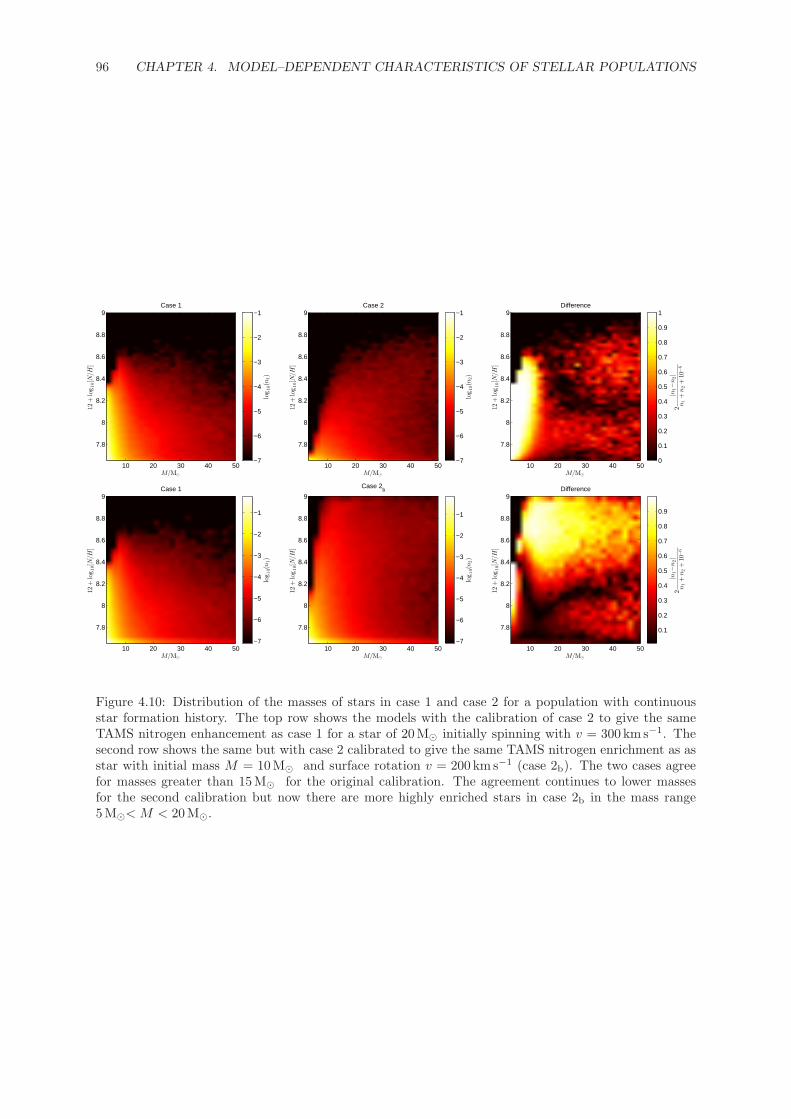
96 CHAPTER 4. MODEL–DEPENDENT CHARACTERISTICS OF STELLAR POPULATIONS
Case 1
M/M�
12+log10[N
/H]
10 20 30 40 50
7.8
8
8.2
8.4
8.6
8.8
9
log10(n
1)
−7
−6
−5
−4
−3
−2
−1Case 2
M/M�
12+log10[N
/H]
10 20 30 40 50
7.8
8
8.2
8.4
8.6
8.8
9
log10(n
2)
−7
−6
−5
−4
−3
−2
−1Difference
M/M�
12+log10[N
/H]
10 20 30 40 50
7.8
8
8.2
8.4
8.6
8.8
9
2|n
1−n2|
n1+n2+10
−6
0
0.1
0.2
0.3
0.4
0.5
0.6
0.7
0.8
0.9
1
Case 1
M/M�
12+log10[N
/H]
10 20 30 40 50
7.8
8
8.2
8.4
8.6
8.8
9
log10(n
1)
−7
−6
−5
−4
−3
−2
−1
Case 2b
M/M�
12+log10[N
/H]
10 20 30 40 50
7.8
8
8.2
8.4
8.6
8.8
9
log10(n
2)
−7
−6
−5
−4
−3
−2
−1
Difference
M/M�
12+log10[N
/H]
10 20 30 40 50
7.8
8
8.2
8.4
8.6
8.8
9
2|n
1−n2|
n1+n2+10
−6
0.1
0.2
0.3
0.4
0.5
0.6
0.7
0.8
0.9
Figure 4.10: Distribution of the masses of stars in case 1 and case 2 for a population with continuousstar formation history. The top row shows the models with the calibration of case 2 to give the sameTAMS nitrogen enhancement as case 1 for a star of 20M� initially spinning with v = 300 km s−1. Thesecond row shows the same but with case 2 calibrated to give the same TAMS nitrogen enrichment as asstar with initial mass M = 10M� and surface rotation v = 200 km s−1 (case 2b). The two cases agreefor masses greater than 15M� for the original calibration. The agreement continues to lower massesfor the second calibration but now there are more highly enriched stars in case 2b in the mass range5M�< M < 20M�.

4.3. RESULTS 97
Case 1Z
v/km s–1
12+
log 1
0[N
/H]
0 100 200 300 400 500
7
7.5
8
8.5
log 1
0(n
1)
−6
−5
−4
−3
−2
Case 2Z
v/km s–1
12+
log 1
0[N
/H]
0 100 200 300 400 500
7
7.5
8
8.5
log 1
0(n
2)
−6
−5
−4
−3
−2
Difference
v/km s–1
12+
log 1
0[N
/H]
0 100 200 300 400 500
7
7.5
8
8.5
2|n
1−n2|
n1+
n2+
10−6
0.1
0.2
0.3
0.4
0.5
0.6
0.7
0.8
0.9
Figure 4.11: Hunter diagrams for populations of stars undergoing continuous star formation at LMCmetallicity. The two populations are qualitatively similar to the populations at solar metallicity. Wehave also plotted the LMC stars observed by Hunter et al. (2009). Case 1Z predicts a very confineddistribution of enriched stars, whereas case 2Z predicts a much wider spread of enrichment. The stars atthe left–hand edge of the diagram can’t be explained by rotational mixing alone.

98 CHAPTER 4. MODEL–DEPENDENT CHARACTERISTICS OF STELLAR POPULATIONS
Fig. 4.11.
We see that the qualitative distribution of stars in the simulated population is similar
to the solar metallicity populations. Case 1Z produces a much more well–defined band
of enriched stars whereas case 2Z produces fewer enriched stars that have a much greater
spread in abundance. If we consider the mass–dependence of the rotational mixing we
find a similar decline in the amount of mixing in case 2Z compared to case 1Z for stars
less massive than 20 M�. As in chapter 3, we find that the amount of mixing in stars
above this mass is higher in case 2Z than in case 1Z. In fact, the mixing in case 1Z
decreases slightly for higher–mass stars. This means that, as in section 4.3.5, an increase
in the mixing in case 2Z is unlikely to produce a better correlation between the two cases.
However, owing to the IMF, there are many more stars less massive than 20 M� in the
population and so case 1 produces many more enriched stars than case 2Z.
In Fig. 4.11 we have also plotted those LMC stars for which the nitrogen abundances
have been determined by Hunter et al. (2009). As remarked by Hunter et al. (2009), there
are many highly enriched, slowly rotating stars that are not explained by either model of
rotational mixing. These are addressed in chapter 5. For the remainder of observed stars
we see a trend of increasing enrichment for higher rotation rates. On initial inspection,
case 1Z fits the VLT–FLAMES data much more closely than case 2Z. However, selection
effects are important and we consider these in section 4.3.7.
4.3.7 Selection effects in the VLT–FLAMES survey
The most common data set used to test rotational mixing in massive stars is the VLT–
FLAMES survey of massive stars (Dufton et al., 2006; Evans et al., 2005, 2006) owing
to the number of stars sampled and the detailed determination of surface composition.
We repeated our population synthesis as in section 4.3.6 for a continuous population of
LMC–metallicity stars but we have included the selection effects which affect the stars
in the VLT–FLAMES survey so that we may compare the distributions more directly
with those found by Hunter et al. (2009). The selection criteria we used are that of the
cluster N11 in the LMC. For a detailed description see Brott et al. (2011b). Stars are
excluded if their visual magnitude is greater than 15.34, if they are hotter than 35,000 K,
if their surface gravity is less than 103.2 cm s−2 or they are rotating faster than 90% of
their critical rotation rate. In addition, a random error is applied to log10[N/H] selected
randomly from a Gaussian with standard deviation σ = 0.2.
The simulated population produced after we apply the selection effects is shown in
Fig. 4.12 along with the LMC stars data of Hunter et al. (2009). We show the population
in cases 1Z, 2Z and 2Zb (the LMC analogue of case 2b with the calibration described in
section 4.3.5). We see that, contrary to our discussion in section 4.3.6, the differences
between the various models are now far less apparent. Compared with the other two
cases, case 2Z predicts many more less–enriched fast rotators than are observed and the
amount of mixing is insufficient to match the observed band of enriched stars. Compared

4.3. RESULTS 99
Case 1Z
v/km s–1
12+
log 1
0[N
/H]
0 100 200 300 400
7
7.5
8
8.5
9
log 1
0(n
1)
−6
−5
−4
−3
−2
Case 2Z
v/km s–1
12+
log 1
0[N
/H]
0 100 200 300 400
7
7.5
8
8.5
9
log 1
0(n
2)
−6
−5
−4
−3
−2
Case 2Zb
v/km s–1
12+
log 1
0[N
/H]
0 100 200 300 400
7
7.5
8
8.5
9
log 1
0(n
3)
−6
−5
−4
−3
−2
Figure 4.12: Hunter diagrams for populations of stars undergoing continuous star formation at LMCmetallicity for a number of different models with selection effects applied as described in section 4.3.7.Populations have been simulated for cases 1Z, 2Z and 2Z
b . The populations are qualitatively similar to thepopulations at solar metallicity. We have also plotted the LMC stars observed by Hunter et al. (2009).The slowly–rotating, highly–enriched stars at the left–hand edge of the diagram cannot be explained byrotational mixing alone.

100 CHAPTER 4. MODEL–DEPENDENT CHARACTERISTICS OF STELLAR POPULATIONS
10 20 30 40 50 60 700
0.02
0.04
0.06
0.08
0.1
Case 1Z
M/M�
n1
Figure 4.13: Distribution of masses in a simulated population of case–1Z stars at LMC metallicity withthe inclusion of selection effects. The distribution is very similar in each case. We see that the distributionpeaks strongly around 12M�.

4.4. CONCLUSIONS 101
with section 4.3.6, cases 1Z and 2Zb now both show a similarly good fit to the data. In both
cases the band of predicted enriched stars is matched well by the observations. However,
we note that we would expect to see a number of stars with 12 + log10[N/H] > 8. The
number of predicted stars in this range is greater for case 2Zb than case 1Z . If we were
to reduce the amount of mixing we would get too little nitrogen enrichment in stars
with v < 200 km s−1. This effect may be a result of the difficulty of measuring nitrogen
abundances in this region but is otherwise difficult to resolve. A further increase in
the mixing would exacerbate the problem that the upper bound to enrichment at rapid
rotation is too high. A decrease in the mixing would mean that the band of enriched
stars in the simulated population is less likely to produce a good fit to the model and
would leave observed slowly–rotating, moderately–enriched stars that cannot be explained
through the theoretical models.
Unfortunately, the mass dependence of the models is not well reflected in the VLT–
FLAMES populations. With the selection effects described, the masses of the LMC–
metallicity sample are confined between 10 M� and 20 M� as shown in Fig. 4.13. We
find a similarly narrow range when we consider Galactic stars under similar selection
effects. Therefore, any simulated population where we include the selection effects of
VLT–FLAMES captures the rotational–dependence of the model but for only a small
fraction of the mass–dependence which is where we have found the biggest differences
between our two cases.
4.4 Conclusions
Rotation has many effects on stellar evolution. Some of these, such as that on the sur-
face temperature, are because of rotation but only vary significantly between different
models towards the end of the main sequence. Others, such as that on the surface rota-
tion velocity, may evolve differently throughout the main sequence according to different
models but do not produce significant changes in the distribution of stars in a simulated
population. Therefore these properties alone are largely unhelpful to distinguish between
the different implementations of rotation in stellar models.
It has been observed that the surface abundances of several chemical elements change
significantly because of rotation. The degree to which this happens in the theoretical
models strongly depends on which particular model for stellar rotation is used and which
constraints are used to calibrate them. Recently, the Hunter diagram has been the
favoured diagnostic tool for analysing stellar rotation because it shows a clear connection
between the surface rotation of a star and its surface enrichment. Our model based on
that of Talon et al. (1997), case 1, shows a similar order of magnitude enrichment for all
masses. On the other hand our model based on that of Heger et al. (2000), case 2, shows
a steep decline in the amount of enrichment around 15 M�. We can account for this to a
degree by adjusting the calibration of the models but we see that increasing the mixing

102 CHAPTER 4. MODEL–DEPENDENT CHARACTERISTICS OF STELLAR POPULATIONS
in case 2, so that low–mass stars show similar enrichment to those of case 1, then leads to
a much higher maximum enrichment for a case–2 population than a case–1 population.
This suggests that studies should focus on stars either side of this mass limit.
Because the two models are very different for different mass ranges, the effective gravity
is a sensible tool to investigate the mass–dependence of the mixing strength. It is very
difficult to self–consistently infer the mass of a star from a luminosity–temperature–
rotation relation because any such relation depends on the model used for rotation.
The effective gravity however can be derived directly from spectra and, despite some
degeneracy, there is a strong relation between it and the stellar mass. This can be
usefully applied to the study of rotational mixing. We have shown that there are very
clear differences between the synthetic populations produced by each model when nitrogen
enrichment is plotted against surface gravity. In the case of a population in which all the
stars have the same age, they are confined to a very specific region. Stars with surface
gravity below a certain limit evolve into giants and beyond on a short timescale compared
to their main–sequence lifetime. Stars with surface gravity above another limit are less
massive and have not had long enough to become enriched. This effect persists even in
the case of a population of stars with continuous star formation. Case 1 predicts that
nitrogen is enriched over a narrower range of surface gravities than case 2. We see that
case 1 produces many more moderately enriched stars than case 2 but the maximum
enrichment in case 1 is lower than in case 2.
We have also shown that similar trends appear at different metallicities. We simulated
populations in both cases with continuous star formation history at LMC metallicity. The
qualitative distribution of stars in each case was similar to that at Galactic metallicity.
Case 1Z still produced a confined band of enriched stars in the Hunter diagram, whereas
case 2Z produced a much greater spread. Case 1Z also produced many more highly–
enriched stars than case 2Z although the maximum enrichment in case 2Z was higher
than in case 1Z. Similarly to solar metallicity, this is because of the mass dependence of
the mixing in each case. The decline in the amount of mixing in case 2Z begins at higher
masses at low metallicity (20 M� at LMC rather than 15 M� at solar metallicity) and
the mixing in stars above this mass is relatively constant for stars in case 2Z, whereas
case–1Z stars show slightly less enrichment as the mass of stars increases. This may
not be indicative of the strength of the rotational mixing but more that, because the
main–sequence lifetime of the stars decreases with increasing mass, there is less time to
transport nitrogen from the core to the surface.
When we compare the simulated populations to the LMC–metallicity stars in the VLT–
FLAMES survey we find that both cases 1Z and 2Zb , which uses the second calibration
for case 2 described in section 4.3.5, give a reasonable fit to the observed data and it
is difficult to determine which fits the data more closely. Unfortunately the range of
initial masses that remain in the simulated samples after we apply the selection effects
is extremely narrow, between 10 M� and 20 M� in the LMC populations. This means

4.4. CONCLUSIONS 103
that it is difficult to observe the large difference in the mass–dependence of the models.
Hence, a close fit between the Hunter diagrams for a simulated population and the data
of the VLT–FLAMES survey is a useful test of models for rotational mixing but cannot
establish the validity of a model by itself. As we have seen, models for rotational mixing
with very different mass–dependencies can reproduce similarly good fits to the current
data. Whilst, in the future, determinations of the nitrogen abundance in a wider mass–
range of stars may help solve this problem, it is likely that examining the enrichment and
depletion of other elements will be necessary. For example, Brott et al. (2011a) look at
the effect of rotation on the surface Boron abundance. Different initial rotation velocity
distributions may also have a significant effect on the simulated populations.
Despite sharing many similar features, it is unreasonable to expect that two different
models for stellar rotation can produce identical qualitative results for an extended range
of masses, rotation rates and metallicities. We have shown that, whilst the two models
agree for stars more massive than 15 M�, there is much less agreement for less massive
stars. Furthermore, we have only thus far made a comparison of two particular models
for stellar rotation chosen from the many available. In particular we haven’t included
models based around the Taylor–Spruit dynamo (Spruit, 2002) such as that investigated
by Brott et al. (2011b) up to this point. Whilst this is a similar model to that of Heger
et al. (2000) it produces very different results owing to the inclusion of magnetic fields.
We examine the effect of magnetic fields in chapter 5. Whilst the marginally better fit
of case 1 suggests that models in which meridional circulation is treated advectively and
diffusion comes solely from hydrodynamic instabilities are more realistic, the difference
is still not convincing and the results of Brott et al. (2011b) also produce a reasonable fit
to observed LMC stars. To distinguish between these models, and others, it is necessary
to continue with this analysis and extend it to different masses and metallicities as more
data becomes available.

104 CHAPTER 4. MODEL–DEPENDENT CHARACTERISTICS OF STELLAR POPULATIONS

105
Magnetism, as you recall from physics class, is
a powerful force that causes certain items to
be attracted to refrigerators. (Dave Barry)
5Stellar evolution of massive stars with a radiative
alpha–omega dynamo
5.1 Introduction
The study of rotation in the radiative zones of stars is strongly coupled with the evolution
of magnetic fields. Observation of stellar magnetic fields is difficult but a number of
magnetic O and B stars have been discovered (Donati et al., 2001, 2002, 2006a,b; Grunhut
et al., 2011; Neiner et al., 2003). Combined with this, a number of chemically peculiar A
and B stars (known as Ap and Bp stars respectively) with surface field strengths up to
20 kG have been identified (e.g. Bagnulo et al., 2004; Borra and Landstreet, 1978; Hubrig
et al., 2005). We direct the reader to Mathys (2009) for a review. These large–scale
fields tend to have simple geometries and there is debate over whether they arise from
fossil fields present during a star’s formation (Alecian et al., 2008; Cowling, 1945) or
from a rotationally–driven dynamo operating in the radiative zone of the star (Maeder
and Meynet, 2004; Spruit, 1999). In this chapter we focus on the latter but we give
consideration to whether a fossil field can be sustained throughout the stellar lifetime.
In low–mass stars, where the outer region is convective, magnetic fields are expected to
be formed in a strong shear layer at the base of the convection zone and then transported
to the surface by convection and magnetic buoyancy (Nordhaus, 2010). In radiative
zones there is no strong bulk motion to redistribute magnetic energy. In most dynamo
models, magnetic flux is redistributed by magneto–rotational turbulence (Spruit, 2002).
This turbulence is also responsible for driving the generation of large–scale magnetic flux.
This is the α–effect (e.g. Brandenburg, 2001) which applies to both poloidal and toroidal

106 CHAPTER 5. STELLAR EVOLUTION WITH AN ALPHA–OMEGA DYNAMO
components, although in rotating systems shear is generally more effective at producing
toroidal field from the poloidal component and so the α–effect is needed for the poloidal
field only. The toroidal field is instead maintained by the conversion of poloidal field into
toroidal field by differential rotation. This is commonly referred to as an α–Ω dynamo
(Schmalz and Stix, 1991).
Because observed fields are potentially strong enough to affect chemical mixing and
angular momentum transport, their inclusion in stellar evolution models is essential. Ro-
tation itself is a likely candidate to drive dynamo mechanisms within a star and theoret-
ical models (e.g. Spruit, 1999) have predicted magnetic fields that can produce turbulent
instabilities which dominate the transport of angular momentum. Whilst the purely hy-
drodynamic evolution of the angular momentum distribution in main–sequence stars has
been considered extensively in the framework of one–dimensional stellar evolution calcu-
lations (e.g. Heger et al., 2000; Meynet and Maeder, 2000), magnetic fields have received
far less attention (Brott et al., 2011a; Maeder and Meynet, 2004). The evolution of the
angular momentum distribution and magnetic field strength have a significant effect on
the final fate of a star and its ejecta.
Apart from causing chemical mixing, sufficiently strong magnetic fields are expected
to cause magnetic braking that results in the rapid spin down of rotating magnetic stars
(Mathys, 2004). It has been suggested that magnetic fields might explain the existence
of slowly–rotating, chemically peculiar stars in surveys of rotating stars (Hunter et al.,
2009). We include a model for magnetic braking based on that of ud-Doula and Owocki
(2002) and show the effects it has on the models of magnetic stars.
Many studies of magnetic fields in massive main–sequence stars consider the Tayler–
Spruit dynamo mechanism (Spruit, 2002). This model asserts that pinch–type instabil-
ities (Spruit, 1999; Tayler, 1973) arise in toroidal fields that drive magnetic turbulence
that enforces solid–body rotation. The growth of instabilities is controlled by magnetic
diffusion which ultimately determines the equilibrium strength of the field. This idea
was built upon by Maeder and Meynet (2004) who found that the Tayler–Spruit dynamo
did indeed result in far less differential rotation than in solely hydrodynamic models. It
was also incorporated in the work of Brott et al. (2011a) who compared stellar evolution
calculations based on the Tayler–Spruit dynamo with the data from the VLT–FLAMES
survey of massive stars (e.g. Evans et al., 2005, 2006). They found reasonable agreement
between the observed and simulated samples (Brott et al., 2011b). However, in chapter 4
we found equally good agreement between the data from the VLT–FLAMES survey and
purely hydrodynamic models based on models of Heger et al. (2000) and Meynet and
Maeder (2000).
In the models of of Spruit (2002) and Maeder and Meynet (2004), the magnetic field is
purely a function of the stellar structure and rotation. Whilst it feeds back on the system
via turbulent diffusivities, the magnetic field doesn’t appear as an independent variable
within the system. In this work we have continued along similar lines to Spruit (2002)

5.2. MAGNETIC ROTATING MODEL 107
but have developed a magnetic model where the poloidal and toroidal components are
evolved via advection–diffusion equations derived from the induction equation. These are
similar in form to the angular momentum evolution equation. The magnetic field and
angular momentum evolution are coupled by turbulent diffusivities, magnetic stresses
and conversion of poloidal field into toroidal field by differential rotation. The dynamo
is completed by regeneration of magnetic flux by a simple α–Ω dynamo. We look at how
the predicted surface magnetic field varies with age and rotation rate for a range of initial
masses and how a simulated population of magnetic stars compares to the data from the
VLT–FLAMES survey of massive stars (Dufton et al., 2006). We also consider how our
model behaves with a strong initial fossil field but without the action of a dynamo.
In section 5.2 we briefly review the model we use to simulate the magnetic fields
including the equations for the α–Ω dynamo and magnetic braking. For the full details
we direct the reader to section 2.4. In section 5.3 we look at the predictions of the model
for a range of stellar masses and initial rotation rates and how simulated populations
compare with observations and in section 5.4 we present a discussion of the results and
our conclusions.
5.2 Magnetic rotating model
In order to simulate the magnetic field in stellar interiors we build on the code rose
(Potter et al., 2012) described in section 2.3.6. We briefly review our model for magnetic
fields in rotating stars in this section. For full details we refer the reader to section 2.4.
We assume the magnetic field, B takes the form
B = Bφ(r, θ)eφ + ∇× (A(r, θ)eφ). (5.1)
By substituting this into the induction equation (c.f. equation (2.33)) and performing a
suitable spherical average we get the equations
∂Bφ
∂t= A
∂Ω
∂r− 6
5rV Bφ − 1
10rUBφ + r
∂
∂r
(η
r4
∂
∂r(r3Bφ)
)(5.2)
and∂A
∂t=
3V
2rA − U
8r
∂
∂r(Ar) +
8α
3πBφ +
∂
∂r
(η
r2
∂
∂r(r2A)
), (5.3)
where the α term represents the regeneration of the poloidal field by magnetic turbu-
lence. The turbulent diffusion coefficient Dmag represents transport of magnetic flux by
turbulence owing to magnetic instabilities. With the inclusion of magnetic forces, the
angular momentum evolves according to
∂(r2Ω)
∂t=
1
5ρr2
∂(ρr4ΩU)
∂r+
1
4πr
∂
∂r(rABφ) +
1
ρr2
∂
∂r
(ρDtotr
4 ∂Ω
∂r
). (5.4)
The diffusion coefficient Dtot includes the diffusion of angular momentum by Kelvin–

108 CHAPTER 5. STELLAR EVOLUTION WITH AN ALPHA–OMEGA DYNAMO
Helmholtz instabilities and convection as discussed in chapters 3 and 4 as well as addi-
tional turbulent transport as a result of magnetic instabilities. The magnetic diffusivity,
η, is
η = r2Ω(ωA
Ω
)2(
Ω
N
)1/2(K
r2NT
)1/2
. (5.5)
where ωA is the Alfven frequency and N is the Brunt–Vaisala and K is the thermal
diffusivity. The chemical composition of the star evolves in radiative zones according to
the equation
∂Xi
∂t=
1
r2
∂
∂r
(PrcDtotr
2 ∂Xi
∂r
), (5.6)
where Prc is the chemical Prandtl number. Similarly we take the magnetic diffusivity to
be η = Prm Dmag where Prm is the magnetic Prandtl number.
The dynamo efficiency is given by
α = γrωAΩq
N, (5.7)
where q = ∂ ln Ω∂ ln r
. Owing to magnetic braking, angular momentum is lost from the star at
a rate given by
dHtot
dt= 4πR4ρDtot
(∂Ω
∂r
)R
, (5.8)
where dHtot
dtis the total rate of angular momentum loss from the star and is given by
dHtot
dt= R2
AΩM = σ2Jsurf . (5.9)
The Alfven radius is RA, σ = RA
Rand Jsurf is the specific angular momentum at the
surface of the star. The parameter σ is evaluated by
σ2 =
√B2∗R2
Mvesc
. (5.10)
There are four free parameters in this model. The parameter Cm affects the overall
strength of the turbulent diffusivity. The magnetic and chemical Prandtl numbers, Prm
and Prc respectively, define the ratio between the diffusion coefficient for angular momen-
tum transport and the diffusion coefficients for the magnetic field and chemical transport.
Finally, γ affects the efficiency of the magnetic dynamo.
5.3 Results
We simulated a grid of models with masses 4 < M/ M�< 24 and initial rotation rates
0 < vini/km s−1 < 600, except where the initial rotation rate is greater than the critical

5.3. RESULTS 109
5 10 15 20 250
100
200
300
400
500
600
700
M/M�
v/km
s–1
B/G
0
200
400
600
800
1000
1200
1400
1600
1800
Figure 5.1: Grid of models considered in section 5.3. The colour of each point indicates the surface fieldstrength at the zero–age main sequence.

110 CHAPTER 5. STELLAR EVOLUTION WITH AN ALPHA–OMEGA DYNAMO
rotation rate of the star. All of the models described are at LMC metallicity as used
by Brott et al. (2011a). We set Cm = 1 and Prm = 1. We also set γ = 10−15 which
results in a maximum field strength across the whole population of B ≈ 20 kG. The
maximum terminal–age main–sequence (TAMS) nitrogen enrichment in the simulated
magnetic population, including observational constraints, is matched with the maximum
enrichment in the slowly rotating population of Hunter et al. (2009). This gives Prc =
0.01. In each model the rotation and magnetic field were allowed to relax to equilibrium
at the zero–age main sequence (ZAMS). The grid of initial models is shown in Fig. 5.1
which also shows the ZAMS surface field strength in each model. We will look at this in
more detail in section 5.3.3.
5.3.1 Magnetic field evolution
Owing to the strong magnetically–induced turbulence, the toroidal field behaves roughly
as Bφ ∝ r−3 and the poloidal field behaves as A ∝ r−2 so both are much stronger towards
the core than at the surface of the star as shown in Fig. 5.2. The toroidal field falls to zero
within a very narrow region near the surface of the star to meet the boundary conditions.
The strength of the toroidal field predicted is around nine orders of magnitude larger
than the poloidal field. This is because the Ω–effect, the conversion of poloidal field into
toroidal field by differential rotation, is much stronger than the α–effect which regenerates
the poloidal field. We take the surface value of the field to be the strength of the toroidal
field just below the boundary layer. If we were instead to take the poloidal field, we
would need a larger value of γ to produce a stronger field. In this case the toroidal field is
around six orders of magnitude larger than the poloidal field. So a surface poloidal field
of 103 G would correspond to a toroidal field of 109 G just below the surface. The fields
then increase by several orders of magnitude towards the core. Not only do these field
strengths seem unreasonably energetic but also the magnetic stresses result in cores that
are spinning near or above break–up velocity. However, spectropolarimetric observations
have concluded that the large–scale structure of the external magnetic fields of massive
stars are largely dipolar so there must be some mechanism for converting the toroidal
field into poloidal field at the surface. It is likely that the stellar wind stretches the field
lines in the radial direction, changing the toroidal field to a radial geometry as material
is ejected from the stellar surface (Parker, 1958).
Owing to the very large value for Dcon predicted from mixing–length theory, the pre-
dicted field is extremely weak within the convective core. This is somewhat at odds with
our observations in the Sun where large–scale magnetic flux can be transported through
a convective region without being destroyed. It may be that convection is better treated
by an anisotropic diffusivity. It has little effect on the magnetic field in the radiative
zone though so does not strongly affect our model for massive stars. We therefore leave
further consideration of this effect for future work.
We first consider models in the absence of magnetic braking in order to distinguish

5.3. RESULTS 111
10-8
10-7
10-6
10-5
10-4
10-3
10-2
0 1 2 3 4 5 6
(A/r
)/G
r/R�
t/tms=0t/tms=0.25t/tms=0.5
t/tms=0.75t/tms=1
103
104
105
0 1 2 3 4 5 6
B/G
r/R�
t/tms=0t/tms=0.25t/tms=0.5
t/tms=0.75t/tms=1
Figure 5.2: Evolution of the magnetic field in a 5M� star initially rotating at 300 km s−1 withoutmagnetic braking. The top plot shows the magnetic potential and the bottom plot shows the toroidalfield. The α–effect produces a weak poloidal field which is efficiently converted into toroidal field bydifferential rotation. For each component, the field strength is approximately three orders of magnitudesmaller at the surface than the core. The ratio of the toroidal and poloidal field strengths is of theorder 109.
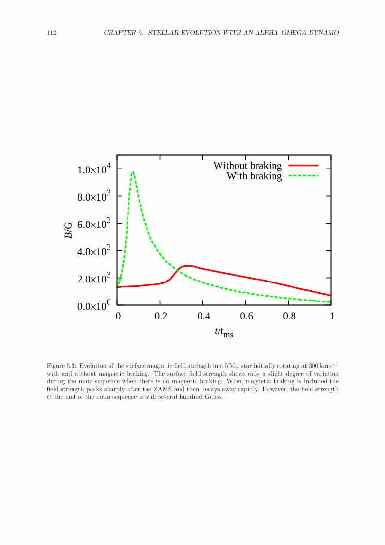
112 CHAPTER 5. STELLAR EVOLUTION WITH AN ALPHA–OMEGA DYNAMO
0.0×100
2.0×10³
4.0×10³
6.0×10³
8.0×10³
1.0×10⁴
0 0.2 0.4 0.6 0.8 1
B/G
t/tms
Without brakingWith braking
Figure 5.3: Evolution of the surface magnetic field strength in a 5M� star initially rotating at 300 km s−1
with and without magnetic braking. The surface field strength shows only a slight degree of variationduring the main sequence when there is no magnetic braking. When magnetic braking is included thefield strength peaks sharply after the ZAMS and then decays away rapidly. However, the field strengthat the end of the main sequence is still several hundred Gauss.

5.3. RESULTS 113
evolutionary effects owing to the dynamo from those caused by braking. In this case,
although the surface field only exhibits a small degree of variation (Fig. 5.3), the magnetic
field inside the star becomes significantly stronger during the course of the main sequence.
The surface magnetic field reaches a peak strength and then weakens towards the end of
the main sequence. However, this change is always within a factor of three of the ZAMS
value. This is consistent with the model of Tout and Pringle (1996) in which Ae/Be stars
tap rotational energy early in their lives. The enhancement of the field inside the star
is largely because the Brunt–Vaisala frequency decreases as the star expands during the
main sequence. It is also partly because the amount of differential rotation increases as
a result of the changing hydrostatic structure of the star.
We might intuitively expect that the spin down of the star owing to magnetic braking
would cause the magnetic field to decay rapidly and this is true later in the life of the
star. However, the inclusion of magnetic braking first leads to a significant enhancement
of the magnetic field shortly after the ZAMS. When braking is included, the loss of angular
momentum from the surface is so fast that diffusion of angular momentum cannot prevent
a build up of shear within the radiative envelope. This drives additional generation of
magnetic flux through the α–Ω dynamo and actually causes a much stronger peak field
than without magnetic braking. The magnetic diffusion eventually reduces the amount
of differential rotation and the magnetic spin down results in a weaker dynamo and faster
rate of field decay. However, the field remains sufficiently large throughout the main
sequence that the rate of chemical transport is still large enough to cause a significant
amount of nitrogen enrichment. We discuss this further in section 5.3.6. Although the
eventual decay of the surface field in the presence of magnetic braking is quite rapid, the
field strength at the end of the main sequence is still several hundred Gauss. This is
consistent with the observation that all chemically peculiar Ap stars have strong fields
(Auriere et al., 2007).
5.3.2 Effect on angular momentum distribution
The effect of the magnetic field on the angular momentum distribution of a star has
profound implications for its chemical evolution and the properties of its remnant. Shear
arises in stars mostly as a result of changes in the structure from ongoing evolution and
mass loss. Rotation also causes meridional circulation in stars. This contributes to the
shear as we discussed in section 2.3.2. In the magnetic case, where magnetic braking is
included, meridional circulation dominates over the magnetic stresses at the ZAMS for
almost the entire star. For a 5 M� star initially rotating at 300 km s−1 the meridional
circulation is approximately six orders of magnitude stronger in the outer layers than the
magnetic stresses at the ZAMS. Through most of the envelope the difference is between
one and three orders of magnitude. However, when the magnetic field grows rapidly
shortly after the ZAMS and magnetic braking begins to rapidly spin down the star this
reverses and the magnetic stresses become much more important than the meridional

114 CHAPTER 5. STELLAR EVOLUTION WITH AN ALPHA–OMEGA DYNAMO
0.0×100
2.0×10³
4.0×10³
6.0×10³
8.0×10³
1.0×10⁴
1.2×10⁴
0 0.2 0.4 0.6 0.8 1
B/G
t/tms
4M�6M�
10M�
Figure 5.4: Evolution of the surface magnetic field strengths in 4M�, 6M� and 10M� stars initiallyrotating at 300 km s−1 with an α–Ω dynamo and magnetic braking. The maximum field strength is muchgreater in less massive stars. For all masses of star, the field strength increases sharply at the start ofthe main sequence owing to the rapid loss of angular momentum at the surface because of magneticbraking. This causes differential rotation which drives additional flux generation by the dynamo. Thispeak occurs later for more massive stars both in absolute time and as a fraction of their main–sequencelifetime. Following this, the field decays rapidly over the remainder of the main sequence.
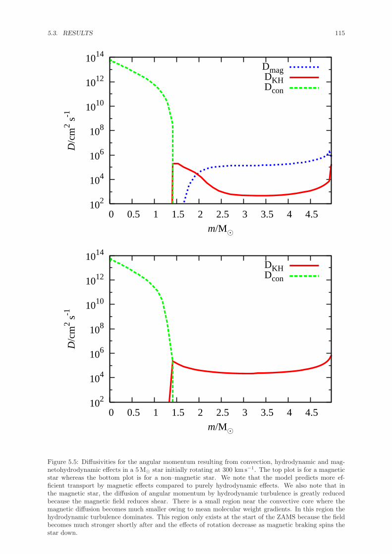
5.3. RESULTS 115
102
104
106
108
1010
1012
1014
0 0.5 1 1.5 2 2.5 3 3.5 4 4.5
D/c
m2 s
-1
m/M�
DmagDKHDcon
102
104
106
108
1010
1012
1014
0 0.5 1 1.5 2 2.5 3 3.5 4 4.5
D/c
m2 s
-1
m/M�
DKHDcon
Figure 5.5: Diffusivities for the angular momentum resulting from convection, hydrodynamic and mag-netohydrodynamic effects in a 5M� star initially rotating at 300 km s−1. The top plot is for a magneticstar whereas the bottom plot is for a non–magnetic star. We note that the model predicts more ef-ficient transport by magnetic effects compared to purely hydrodynamic effects. We also note that inthe magnetic star, the diffusion of angular momentum by hydrodynamic turbulence is greatly reducedbecause the magnetic field reduces shear. There is a small region near the convective core where themagnetic diffusion becomes much smaller owing to mean molecular weight gradients. In this region thehydrodynamic turbulence dominates. This region only exists at the start of the ZAMS because the fieldbecomes much stronger shortly after and the effects of rotation decrease as magnetic braking spins thestar down.

116 CHAPTER 5. STELLAR EVOLUTION WITH AN ALPHA–OMEGA DYNAMO
0.0×100
5.0×10⁻⁵
1.0×10⁻⁴
1.5×10⁻⁴
2.0×10⁻⁴
0 1 2 3 4 5
Ω/s
-1
m/M�
t/tms=0t/tms=0.25t/tms=0.5
t/tms=0.75t/tms=1
0.0×100
5.0×10⁻⁵
1.0×10⁻⁴
1.5×10⁻⁴
2.0×10⁻⁴
0 1 2 3 4 5
Ω/s
-1
m/M�
t/tms=0t/tms=0.25t/tms=0.5
t/tms=0.75t/tms=1
10-9
10-8
10-7
10-6
10-5
10-4
0 1 2 3 4 5
Ω/s
-1
m/M�
t/tms=0t/tms=0.25t/tms=0.5
t/tms=0.75t/tms=1
Figure 5.6: Evolution of the angular momentum distribution in a 5M� star initially rotating at300 km s−1. The top plot is for a non–magnetic star, the middle plot is for a magnetic star withoutbraking and the bottom plot is for a magnetic star with braking. In magnetic stars without braking, thestrong magnetic turbulence results in much less shear than the non–magnetic equivalent. Stronger dif-fusion in the magnetic stars also leads to far less differential rotation between the core and the envelope.This causes higher surface rotation in the non–braked magnetic star compared to the non–magnetic star.When braking is introduced to the magnetic star it spins down rapidly. The angular momentum lossfrom the surface leads to a much higher degree of differential rotation in the magnetic star with brakingcompared to the magnetic star without braking.

5.3. RESULTS 117
circulation for the remainder of the main sequence. As we see in Fig 5.4, this peak
occurs later for more massive stars as a fraction of main–sequence lifetime and so the
meridional circulation can dominate for longer. Therefore, whilst it is true that the
meridional circulation has little effect on the evolution of magnetic stars for most of the
main sequence, it is not necessarily true close to the ZAMS.
Apart from the physical effects that produce shear within the radiative envelope the
other major factor that affects the angular momentum distribution is the strength of the
turbulent diffusion. We have plotted the major diffusion coefficients at the ZAMS for
a 5 M� star initially rotating at 300, km s−1 in Fig. 5.5. The overall diffusion coefficient
predicted by the magnetic model is significantly larger than produced by hydrodynamic
turbulence alone. We note that DKH ∝(
∂Ω∂r
)2predicted in the magnetic model is signifi-
cantly lower than in the non–magnetic model. Whilst magnetic stresses should produce
more shear than in the non–magnetic model, the diffusion coefficient is sufficiently high
to cause an overall reduction in shear. This is illustrated in Fig. 5.6 where we have
plotted the evolution of the angular momentum distribution for the same star without a
magnetic field, with a magnetic field but without braking and with both a magnetic field
and braking. There is a small region near the convective core in the magnetic star where
the magnetic diffusion becomes much smaller owing to mean molecular weight gradients.
In this region the hydrodynamic turbulence dominates. This region only exists at the
start of the ZAMS because the field becomes much stronger shortly after and the effects
of rotation decrease as magnetic braking spins the star down.
In Fig. 5.6 we see that, in the magnetic star without braking, there is far less differential
rotation throughout the star than in the non–magnetic star. This also means that the
cores of magnetic stars are likely to be rotating more slowly than non–magnetic stars
even before the effects of braking are included. When braking is included we see much
the same trend except, in the model with magnetic braking, the whole star spins down
rapidly. The typical Alfven radius for this star is approximately 50, meaning that the
rate of angular momentum loss is several thousand times faster than without a magnetic
field. We note that there is far more differential rotation in this star compared with the
magnetic star without braking. This is because of the rapid loss of angular momentum
from the surface of the star.
5.3.3 Mass–rotation relation of the main–sequence field strength
Historically the presence of strong magnetic fields in massive stars has been thought to
be mainly confined to A stars and perhaps some of the lower–mass B stars (Mathys,
2009). This may have been because of the difficulty in observing magnetic effects in the
broad absorption features of more massive stars (Petit and Wade, 2011). However, as
the amount of available data has grown, thanks to surveys such as MiMeS project (e.g.
Wade et al., 2009), it has become clear that this is not caused simply by selection effects.
By applying our model to the grid shown in Fig. 5.1 we are able to track the evolution of

118 CHAPTER 5. STELLAR EVOLUTION WITH AN ALPHA–OMEGA DYNAMO
M/M�
v/km
s–1
5 10 15 20
50
100
150
200
250
300
350
400
450
500
550
B/G
0
200
400
600
800
1000
1200
1400
1600
Figure 5.7: Main–sequence magnetic field strengths for intermediate–mass ZAMS stars at different ro-tation rates. Stars more massive than 15M� have almost no magnetic activity except for a weak fieldin slow rotators. The strongest fields occur in the most rapidly rotating stars with 4 < M/M�< 10.

5.3. RESULTS 119
M/M�
B/G
5 10 15 200
0.2
0.4
0.6
0.8
1
1.2
1.4
1.6
1.8
2x 10
4
log(n1)
−6
−5
−4
−3
−2
−1
Figure 5.8: Simulated masses and magnetic field strengths for a population of stars drawn from thegrid of models shown in Fig. 5.1. The population undergoes continuous star formation, is drawn from aSalpeter IMF and the velocity distribution is Gaussian with mean μ = 145 km s−1 and standard deviationσ = 94 km s−1. The number of stars in each bin as a fraction of the total number of stars is n1. We seethat lower–mass stars support much stronger fields. There is very little magnetic activity in stars moremassive than around 15M�.

120 CHAPTER 5. STELLAR EVOLUTION WITH AN ALPHA–OMEGA DYNAMO
the surface field strength of stars and, in particular, how it varies with mass and rotation
rate. We show this dependence at the ZAMS in Fig. 5.7. It is immediately apparent that
although stars less massive than around 15 M� are able to sustain significant fields, no
significant field is predicted in more massive stars except in very slow rotators. Even for
high–mass, slow rotators the field doesn’t exceed 200 G. The transition between a strong
ZAMS field and no field is sharpest in rapid rotators. This transition is caused by the
interaction between hydrodynamic and magnetic turbulence. If DKH exceeds Dmag for a
sufficiently large region of the radiative envelope, the magnetic field decays exponentially
and cannot be sustained by the dynamo. Because α ∝ ωA, the strength of the dynamo
weakens with the magnetic field. In the case where Dmag is the dominant turbulent
process, this is matched by a greater reduction in the turbulent diffusivity because, for
most of the envelope, Dmag ∝ ω2A. As the diffusivity drops, the field is less efficiently
dissipated and so an equilibrium is reached. When DKH dominates and the field decays
the diffusivity is largely unaffected and so the dynamo continues to weaken causing the
field to completely disappear. At higher masses and rotation rates DKH is larger and
so catastrophic quenching occurs for lower dynamo efficiencies. Assuming that both
instabilities act in the radiative envelope, this explains why magnetic fields are more
likely to be observed in A stars and less frequently in O and B stars.
Given that the magnetic field strength increases sharply after the main sequence before
decaying away exponentially as discussed in section 5.3.1, we consider the distribution
of magnetic field strengths in a population of stars with a continuous distribution of
ages. The population is shown in Fig. 5.8. The population undergoes continuous star
formation, is drawn from a Salpeter IMF and a Gaussian velocity distribution with mean
μ = 145 km s−1 and standard deviation σ = 94 km s−1. We see that magnetic activity is
highest in the least massive stars. As before, stars more massive than around 15 M� show
no magnetic activity. We note that the stars with the strongest fields fall outside the
observational limits of the VLT–FLAMES survey of massive stars (Dufton et al., 2006).
We discuss this further in section 5.3.6.
We therefore predict two distinct populations of stars. The first is a population of
slowly rotating, magnetic and chemically peculiar stars with masses less than 15 M�.
The second is a population of more massive stars that are non–magnetic and follow
the trend discussed by Hunter et al. (2009) and chapter 4, where rotation and nitrogen
enrichment have a strong positive correlation. This is precisely what we observe (Hunter
et al., 2009). We may still observe A stars that are rapidly rotating but not highly
enriched. These stars should still support a strong magnetic field but are sufficiently
young that no chemical enrichment has occurred. These rapidly rotating stars would
be very infrequent owing to the efficient spin down by the magnetic braking. A rapidly
rotating, highly magnetic massive star was observed by Grunhut et al. (2012). The star
has a mass of 5.5 M� and a surface rotation velocity of 290 km s−1 but has a surface field
strength in excess of 10 kG.

5.3. RESULTS 121
4.15 4.2 4.25 4.3 4.35 4.4 4.45 4.5 4.55
log 1
0(L
/L�
)
log10(Teff/K)
4M�
6M�
10M�
Non rotatingRotating, non magnetic
Rotating, magnetic
Figure 5.9: Hertzsprung–Russell diagram for stars with mass 4M�, 6M� and 10M�. The plot shows thepredicted evolution for non–rotating stars, stars initially rotating at 300 km s−1 but with no magneticfield (c.f. case 1 from chapters 3 and 4) and magnetic stars initially rotating at 300 km s−1. In lessmassive stars magnetic braking rapidly spins down the star so the structural effects of rotation are muchless apparent. In more massive stars the effect of braking is much weaker and so the evolution is muchcloser to the rotating, non–magnetic model.
5.3.4 Effect on the Hertzsprung–Russel diagram
Because less massive stars have stronger fields, both magnetically induced mixing and
magnetic braking are much more effective in these stars. Owing to the stronger mag-
netic mixing, chemical transport is more efficient in less massive stars as discussed in
section 5.3.6. As a result, more hydrogen is mixed down into the core of less massive
stars. However, because magnetic braking causes lower–mass stars to spin down very
rapidly, the effects on brightness and temperature that arise from changes in the stellar
structure in rotating stars are far less apparent when magnetic fields are introduced, as
shown in Fig. 5.9. In the 10 M� model we see that the difference between the magnetic
and non–magnetic rotating models is smaller owing to the much weaker field and hence
less rapid spin down. However, in the evolution of the 4 and 6 M� models the magnetic
stars remain barely distinguishable from the evolution of the non–rotating stars.

122 CHAPTER 5. STELLAR EVOLUTION WITH AN ALPHA–OMEGA DYNAMO
102
103
104
105
0 0.2 0.4 0.6 0.8 1
B/G
t/tms
Dynamo-driven fieldFossil field
Figure 5.10: Evolution of two 5M� stars with different magnetic field models. The first star has nomagnetic dynamo (γ = 0) but starts with a very strong initial field (B = 10 kG). The second star usesthe same dynamo model and parameters as described in section 5.2. The star with an active dynamo isable to sustain the field for longer than the star with a fossil field but, owing to magnetic braking, bothfields eventually decay exponentially. The two stars have similar field strengths at the end of the mainsequence.

5.3. RESULTS 123
5.3.5 The lifetime of fossil fields
An alternative to the radiative–dynamo model is that the magnetic field originates in
the material that formed the star. If the protostellar cloud which forms a star is weakly
magnetic, conservation of magnetic energy would result in a very strong main–sequence
field. We call these fossil fields (Braithwaite and Spruit, 2004). In order for the fossil
field model to work, the field must be able to survive the collapse of the protostellar
cloud during the star formation process. The fossil field argument also relies on a stable
field configuration being reached that would avoid destruction on main–sequence lifetimes.
Certain stable configurations have been found in recent years (Braithwaite and Nordlund,
2006) and simulations have suggested that arbitrary field configurations do relax to these
stable states (Mathis et al., 2011). However, simple field configurations are still subject
to the same instabilities as the fields we have generated by dynamo action, in particular
the Tayler instability (Tayler, 1973). There are a number of other instabilities that could
occur in simple field configurations (Parker, 1966) but for now we consider only the Tayler
instability.
We consider two stars, both initially rotating at 300 km s−1. The first star starts on
the ZAMS with a magnetic field of 10 kG but γ = 0 so no dynamo operates. The second
star is a rotating magnetic star with dynamo parameters described in section 5.2. The
evolution of the magnetic fields is shown in Fig. 5.10. In each case, the initial field
undergoes some amplification at first owing to the onset of mass and angular momentum
loss and the subsequent redistribution of angular momentum through the envelope. This
is much more rapid in the case of the fossil field and does not appear in Fig. 5.10. The
field then decays exponentially during the main sequence. We note that although the
star with an operating dynamo is able to prevent the field from decaying for a short time,
once magnetic braking has spun the star down sufficiently, the dynamo can no longer
maintain the field which then decays exponentially. The final field strength is similar in
each case.
Because the fossil field model predicts field evolution similar to that of the dynamo
model it is difficult to argue which model is more physically accurate. However, we
note that the fossil field strength has to be several orders of magnitude larger than the
initial field in the case of a magnetic dynamo in order to reproduce the same final field.
The question remains whether the fossil field argument can produce stars with strong
enough initial fields so that they remain strong enough to influence chemical mixing in
the star during the main sequence. Moss (2003) examined how much magnetic flux could
potentially survive to the ZAMS from the pre–main sequence. He found that a significant
fraction of flux could survive but only if the magnetic diffusivity was sufficiently low.
Above this limit, no flux was expected to survive. The fossil field must also reproduce
the two distinct observed populations in the Hunter diagram, shown in Fig. 5.11, discussed
further in section 5.3.6. One could argue that this depends on the distribution of magnetic
field strengths in protostellar clouds but the fossil field model must then also explain the

124 CHAPTER 5. STELLAR EVOLUTION WITH AN ALPHA–OMEGA DYNAMO
0 100 200 300 4006.6
6.8
7
7.2
7.4
7.6
7.8
8
v/km s–1
12+
log 1
0[N
/H]
log 1
0(T
eff/K
)
4.3
4.35
4.4
4.45
4.5
Figure 5.11: Hunter diagram for the LMC stars observed in the VLT–FLAMES survey of massive stars(Hunter et al., 2009). Stars with surface gravity smaller than log10(geff/cm2 s−1) = 3.2 are classified asgiants and have been excluded. The effective temperature of each star is also shown.
mass–dependent distribution of field strengths observed in massive stars. Thus far we
have come across no arguments that accurately reproduce these features of observed
populations for fossil fields.
5.3.6 Effect on surface composition
The Hunter diagram (Hunter et al., 2009) is a plot of the surface nitrogen abundance
in a star against surface velocity. The VLT–FLAMES survey of massive stars (Dufton
et al., 2006; Evans et al., 2005, 2006) resulted in a significant amount of data on the
nitrogen abundances in rotating stars in a number of samples from the Milky Way and
Magellanic Clouds (Hunter et al., 2009). In particular it was observed that there exists
a class of stars that are slowly rotating (v < 60 km s−1) but exhibit significant nitrogen

5.3. RESULTS 125
v/km s–1
12+
log 1
0[N
/H]
0 100 200 300 400
7
7.2
7.4
7.6
7.8
8
8.2
8.4
log(n1)
−4
−3.8
−3.6
−3.4
−3.2
−3
−2.8
−2.6
−2.4
−2.2
−2
Figure 5.12: Hunter diagram for a population of stars drawn from the grid of models shown in Fig. 5.1.The population undergoes continuous star formation, is drawn from a Salpeter IMF and the velocitydistribution is Gaussian with mean μ = 145 km s−1 and standard deviation σ = 94 km s−1. The numberof stars in each bin as a fraction of the total number of stars is n1. The magnetic model reproduces wellthe two distinct populations of stars observed in the VLT–FLAMES survey. More massive stars whichcannot support a dynamo are enriched by rotational mixing whereas lower–mass stars are spun downrapidly and are enriched by magnetic mixing.

126 CHAPTER 5. STELLAR EVOLUTION WITH AN ALPHA–OMEGA DYNAMO
M/M�
v/km
s–1
5 10 15 20
50
100
150
200
250
300
350
400
450
500
550
B/G
0
100
200
300
400
500
600
Figure 5.13: Distribution of magnetic field strengths with respect to mass and rotation rate for a popu-lation of stars undergoing continuous star formation. The population is drawn from a Salpeter IMF andthe velocity distribution is Gaussian with mean μ = 145 km s−1 and standard deviation σ = 94 km s−1.The gray region is where stars are not observed in the simulated population. Less massive stars areeliminated from the sample because they have insufficient magnitude for detection. The black region isfor stars that appear in the simulated population but have no discernible field. We see that the magneticstars in the sample, responsible for producing the slowly–rotating, enriched stars in Fig. 5.12 come froma narrow region around M = 10M�.

5.3. RESULTS 127
enrichment. It was suggested that these stars are, or once were, magnetic stars. If we
extend the Hunter diagram to consider the effective temperature of each star as shown
in Fig. 5.11 we do not see a significant temperature variation between the two groups
but we note that the mass range of stars in this sample is only 8 < M/M� < 20 and so
we cannot draw any strong conclusions about the relative mass distribution of the two
enriched populations.
The observed distribution of surface abundance anomalies are well reproduced by our
model which predicts magnetic fields only in stars less massive than around 15 M�. The
rest of the stars in the sample continue to evolve as non–magnetic stars as described in
chapter 4. The two distinct populations that we see in Fig. 5.11 are reflected by the
predictions made in section 5.3.3, shown in Fig. 5.12. This shows a simulated population
of stars between 8 M� and 20 M� with our radiative–dynamo model and with magnetic
braking. The mass range is smaller than that of the full grid shown in Fig. 5.1 owing
to the removal of the least and most massive stars because of observational effects. The
population was generated with the population synthesis code starmaker (Brott et al.,
2011b). It behaves exactly as we would expect from the VLT–FLAMES data. The
stars initially have a full spread of rotation rates but the magnetic population spins
down rapidly owing to the effects of magnetic braking. The magnetic field continues to
affect the mixing and these stars become enriched as they age producing a population
of magnetic, slowly rotating, chemically peculiar stars. More massive stars, where an
equilibrium field cannot be supported by the dynamo, evolve as non–magnetic stars with
hydrodynamic turbulence driving the mixing. This produces a second population whose
enrichment increases with rotation rate as modelled in chapter 4. The two populations
are also highlighted in Fig. 5.13 which shows the relationship between field strength, mass
and rotation rate in the simulated population. Most of the stars evolve without magnetic
fields but there is a small region, at the lower mass limit of the sample (M ≈ 10 M�),
where stars are predicted to be magnetic. We note that, because this region is very
narrow, small changes in the boundary between magnetic and non–magnetic evolution
have a significant effect on the number of magnetic stars in the observed sample. It is
possible this effect could be produced by fossil fields as discussed in section 5.3.5 but thus
far there is no way to explain why we see such distinct populations in the VLT–FLAMES
data or why magnetic fields have a higher incidence rate amongst less massive stars.
We also note that those stars in Fig. 5.11 with nitrogen enrichment 6.8 < log10[N/H] <
7.1 and 0 < v/km s−1 < 150 cannot easily be categorized into either group of stars. They
may be low–mass, fast rotators that have been partially spun down by magnetic braking,
low–mass stars that are born with slow rotation or high–mass stars that are born with
slow rotation. These stars evolve along a relatively similar path in the Hunter diagram.

128 CHAPTER 5. STELLAR EVOLUTION WITH AN ALPHA–OMEGA DYNAMO
Cm Prm γ max(
rBφ
A
)max(q) max(Bsurf/G)
1 1 1.93 × 10⁻¹⁶ 4.2 × 10⁹ 1.39 3.06 × 10³
0.1 1 2.40 × 10⁻¹⁸ 1.1 × 10¹¹ 0.96 7.10 × 10²
10 1 3.53 × 10⁻¹⁴ 1.2 × 10⁸ 0.019 1.53 × 10³
1 0.1 1.52 × 10⁻¹⁶ 3.74 × 10⁹ 1.04 7.40 × 10²(2)
0.1 0.1 3.00 × 10⁻¹⁷(3)
10 0.1 1.81 × 10⁻¹⁴ 4.4 × 10⁸ 0.25 1.27 × 10³
1 10 1.04 × 10⁻¹⁴ 8.13 × 10⁸ 0.0089 1.55 × 10³
0.1 10 4.47 × 10⁻¹⁶ 1.95 × 10¹⁰ 0.14 8.92 × 10²
10 10 1.58 × 10⁻¹¹ 2.1 × 10⁷ 0.033 N/a(1)
Table 5.1: The variation of magnetic and stellar parameters with different values for Cm and Prm fora 5M� star initially rotating at 200 km s−1 with magnetic braking. Each model was taken to have thesame equilibrium ZAMS field. The table shows the values of Cm, Prm and γ used for each model as wellas the maximum internal value of the ratio of the poloidal and toroidal field, rBφ
A and q = ∂Ω∂r , taken at
5 × 10⁷yr. Finally the table shows the maximum value of the surface field during the main sequence.We note three special entries in the table. (1) This star evolved quasi–homogeneously and produceda monotonically increasing field well beyond the normal main–sequence lifetime. Therefore defining amaximum main–sequence field was inappropriate. (2) This star evolved normally but we note that fora slightly smaller value of γ we were unable to maintain an equilibrium field. This effect was discussedin section 5.3.3. (3) This star is similar to (2) but in this case we were totally unable to maintain anequilibrium field at the desired strength. We note that for stars (2) and (3), a stronger field can bemaintained provided the dynamo–efficiency is sufficiently large.
5.3.7 Variation with different parameters
The model currently contains four parameters which we may vary independently. If
we include possible recalibration of the Alfven radius by constants of order unity then
this increases to five. We may fix the Alfven radius by ensuring that the population of
enriched magnetic stars is confined to the appropriate band of rotation rates as discussed
in section 5.3.6. We can also set Prc by ensuring that the maximal enrichment of magnetic
stars is the same as in the VLT–FLAMES data also discussed in section 5.3.6. The
remaining three parameters may then be varied so that typical field strengths are of the
order 10 kG, as observed in magnetic Ap stars (Mathys, 2009). This value is subject to
change though given the scarcity of observations of magnetic stars. This still leaves a
high degree of freedom within the model. Up to this point we have used C = Prm = 1
and γ = 10−15 but we consider the effect of varying Cm and Prm by an order of magnitude
in either direction. We ran our 5 M� star initially rotating at 300 km s−1 with magnetic
braking. The effect on a number of parameters is shown in Table 5.1.
For low magnetic Prandtl numbers it is much more difficult to sustain the dynamo.
The same surface field is reproduced with smaller dynamo efficiencies but the minimum
sustainable field strength is larger. In the case of small Cm and small Prm, the field was
completely quenched by the hydrodynamic turbulence as described in section 5.3.3. A
dynamo could be sustained for stronger surface fields but only by increasing the dynamo
efficiency significantly. Even for Cm = 1 we found that for a small reduction in γ the
ZAMS field collapsed.
For higher values of Cm, the diffusion of the magnetic field requires a larger dynamo

5.4. CONCLUSIONS 129
efficiency in order to maintain the same strength field and vice–versa for smaller values of
Cm. For simultaneously large values of Cm and Prm the field keeps growing monotonically
with time during quasi–homogeneous evolution. This is to be expected when the dynamo–
driven mixing becomes very high. Typically we could adjust Prc to compensate.
Regardless of our choice of Cm and Prm, the ratio of the poloidal and toroidal field
strength is well correlated with the dynamo efficiency. Larger values of the dynamo
efficiency lead to a smaller ratio between the two field strengths. This is because of
the form of equations (5.2) and (5.3). Because the two fields have the same diffusion
timescales, their equilibria depend on the regeneration terms. In the case of the poloidal
field this comes from the α–effect and for the toroidal field it comes from the shear. In
all of our models, the α–effect is much weaker than the effect of shear and so the poloidal
field strength is much smaller. However if γ is increased, increasing the regeneration of
the poloidal field but having little direct effect on the toroidal field, the ratio between the
two becomes much smaller.
There are other aspects of the evolution that are much more difficult to explain and
are related to the non–linearities in the model and their coupling to the effects of stellar
evolution on nuclear timescales. We might expect the maximum value of the shear to
always be smaller with higher values of Cm because the angular momentum transport
is more efficient but, while this is true in general, it isn’t a simple relationship. Like-
wise the maximum main–sequence surface field doesn’t seem to correlate with either free
parameter.
In particular, the relative abundance of slow and fast rotating chemically peculiar stars
may be explained by a shift in the position by mass of the cut–off between magnetic stars
and non–magnetic stars discussed in section 5.3.3. The effect of these free parameters on
the position of the cut–off is something we leave for future work.
5.4 Conclusions
Magnetic fields are one of the most mysterious and least understood aspects of stellar
evolution. The first magnetic massive star was discovered over 65 years ago (Babcock,
1947) and yet debate still rages about whether these fields have primordial origin or are
generated by a radiative dynamo acting within the stellar envelope. Models of magnetic
stars must reproduce the observed phenomenon of magnetic A stars with unusual surface
compositions that have much slower rotation rates than the rest of their population
(Mathys, 2004). The data from the VLT–FLAMES survey of massive stars (Evans et al.,
2005, 2006) also supports the idea that there exists a population of stars that are slowly
rotating but have a high degree of nitrogen enrichment (Hunter et al., 2009).
We have presented a simple radiative dynamo model that arises because of the Tayler
pinch–type instability (Tayler, 1973) and is based on the model of Spruit (1999) which
was further developed by Spruit (2002) and Maeder and Meynet (2004). Unlike previous

130 CHAPTER 5. STELLAR EVOLUTION WITH AN ALPHA–OMEGA DYNAMO
work, we have evolved both the poloidal and toroidal fields as independent variables at
each radius in the star coupled to the angular momentum distribution of the star. The
magnetic fields evolve according to a latitudinally–averaged induction equation with the
inclusion of an αΩ–dynamo mechanism derived from mean–field magnetohydrodynamics
(Schmalz and Stix, 1991). We introduce a model for magnetic braking similar to that of
ud-Doula and Owocki (2002). The model depends on a number of parameters, the overall
strength of the magnetic turbulence, the magnetic Prandtl number, the chemical Prandtl
number, the dynamo efficiency and the critical ratio of the kinetic energy to the magnetic
energy, which defines the Alfven radius. The choices of Cm, which affects the strength of
the magnetic turbulence, and Prc have a strong effect on the dynamo efficiency needed
to sustain the field but the relation between these parameters and the internal evolution
of the models is complicated.
In models of the magnetic field, when magnetic braking is not included, the field varies
only by a factor of a few during the main sequence. When we include magnetic braking,
the Alfven radius is typically between 10 and 100 times greater than the stellar radius
and so angular momentum loss is some 103 times greater than from non–magnetic mass
loss alone. The rapid angular momentum loss from the surface drives additional shear
that leads to increased field generation. In magnetic stars with magnetic braking, the
field increases rapidly at the start of the main sequence before decaying exponentially.
The field strengths at the end of the main sequence are predicted to be of order 100 G.
We consider a population of stars with this magnetic model and find two distinct
types of behaviour. For stars more massive than around 15 M� the Kelvin–Helmholtz
turbulence dominates over the magnetic turbulence and a stable field cannot be sustained
by the dynamo. In these cases we see no appreciable field strength during the main
sequence so the stars evolve according to our normal prescription for non–magnetic,
rotating stars. The predicted field strength is stronger for rapid rotators but the overall
strength does not depend strongly on the stellar mass except near the limit at which the
dynamo can sustain the field. Although the magnetic field decays exponentially after
an initial peak, it remains strong enough to have a significant effect on the chemical
evolution of the star. Though the actual mass at which this dichotomy sets in depends
on parameters, the fact it exists is an important consequence of our model.
If we look at the evolution of an artificially strong initial field in the absence of any
dynamo action, but subject to the diffusion that arises from the Tayler (1973) instability,
we find that reproducing the same TAMS field requires an initial field several orders of
magnitude larger than in the presence of a dynamo because any fossil field is predicted to
decay exponentially. The fossil field hypothesis suffers from the problem that we expect
the fields in low–mass stars to decay more than in more massive stars, likely because of
their much longer main–sequence lifetimes. This is opposite to observed trends which
suggest that less massive stars are more likely to support strong fields than more massive
stars Grunhut et al. (2011). This model also offers no explanation as to why we see two

5.4. CONCLUSIONS 131
distinct groups in the Hunter diagram. Both of these issues are well resolved by our
αΩ–dynamo model.
We created an artificial population of stars with the population synthesis code star-
maker (Brott et al., 2011b), including the effects of the α–Ω dynamo and magnetic
braking. The population reflects well the observations of the VLT–FLAMES survey of
massive stars. The survey observed two distinct populations of stars. The first shows
increasing nitrogen enrichment with rotation rate, the second is a class of slow–rotating
stars that exhibit unusually high nitrogen abundances compared to the rest of the pop-
ulation. This distribution of stars is well reproduced by the magnetic model. The fact
that the two very different evolutionary paths arise naturally from the model is very
encouraging to explain why we observe these two classes of star without having to appeal
to the fossil fields argument.
There are still a number of open questions and further refinements that need to be
made to the model. We have evolved a magnetic population of stars with the same initial
velocity distribution as the non–magnetic stars. If the radiative dynamo has a strong
effect on the pre–mainsequence evolution then magnetic braking causes magnetic stars
to reach the ZAMS with significantly slower rotation rates than stars with no significant
field. This is indeed observed in stellar populations (Mathys, 2004). Alecian et al. (2008)
also discovered a number of stars on the pre–main sequence which exhibited significant
magnetic activity. They attribute these to fossil fields by eliminating the possibility that
the fields could be generated by a convective dynamo. However, if a radiative dynamo
operates in these stars it could also be responsible for the generation of the observed
fields. By comparison, the observations of Grunhut et al. (2012) suggest that magnetic
stars may reach the main sequence with significant rotational velocities. If magnetic
stars were born with slower rotation rates than their non–magnetic counterparts then
this would partly explain why the required dynamo efficiency is so small and why the
predicted ratio between the poloidal and toroidal fields is so large. If magnetic stars
were born with lower surface rotation rates then a higher dynamo efficiency would be
needed to produce observed magnetic field strengths. This would reduce the difference
between the α–effect and the Ω–effect and so the ratio of the strengths of the poloidal
and toroidal fields would be closer to unity. Another possible explanation for why the
predicted dynamo efficiency is so small is that we chose the radial coordinate as the
length scale for the dynamo action. In reality a more sensible choice may have been the
length scale of the saturated magnetic instabilities, lr (c.f. equations (2.42) and (2.43)). A
shorter length scale would result in a weaker dynamo and therefore the dynamo efficiency
would need to be higher to sustain the same field strength.
The observed proportion of Ap stars as a fraction of the whole population of A stars
is roughly 10% (Moss, 2001). Our grid of models does not yet extend down to the mass
range for A stars (1.4 < M/ M�< 2.1) and so we cannot yet say whether our population
matches this statistic. We do expect that, given the predicted initial velocity distribution

132 CHAPTER 5. STELLAR EVOLUTION WITH AN ALPHA–OMEGA DYNAMO
of massive stars, the population of A stars should still be dominated by slow rotators
that do not support a radiative dynamo. In the mass range of our simulated population,
over 90% of stars in the sample have surface field strength less than 187 G. This is well
below the limit of 300 G anticipated for the transition to Ap classification (Auriere et al.,
2007). Although our population contains some very massive stars where we expect smaller
field strengths, the form of the IMF ensures that the population is still dominated by
intermediate–mass stars so the figure for A stars is likely to be similar. It is also likely
that below a certain amount of shear, a dynamo does not operate. We have not taken this
into account in our simple model. If it is the case, there may also be a sharp transition
between magnetic and non–magnetic behaviour at low rotation rates.
In our models we have assumed a simple magnetic field geometry. Even if real fields are
generated by dynamo action then they may still relax to stable field configurations such as
those suggested by Braithwaite and Nordlund (2006); Mathis et al. (2011). Further work
is needed to determine how the model might behave differently under these conditions.
Further consideration must also be given to the action of convection on the magnetic
field. Does our diffusive model apply in convective zones and if so is it anisotropic?
Furthermore, can we better constrain the free parameters in the system, including the
efficiency of magnetic braking? Although data on magnetic stars is scarce, a great deal
of progress has been made possible by surveys such as the VLT–FLAMES survey of
massive stars and the MiMeS project. These provide sufficient clues to further constrain
our existing models. Additional progress will no doubt be possible thanks to ongoing
developments in stellar observations from the MiMeS project (Grunhut et al., 2011; Wade
et al., 2009) and additional data on stellar surface compositions through projects such as
the VLT–FLAMES tarantula survey (Evans et al., 2011).

133
All things change; nothing perishes. (Ovid)
6White dwarf magnetic fields in strongly interacting
binaries
6.1 Introduction
Surveys of the galactic white dwarf (WD) population have discovered magnetic field
strengths ranging up to about 109 G (Schmidt et al., 2003). Typically WDs fall into two
categories, those with field strengths of the order 106 G or higher and those with fields
weaker than around 105 G. We focus here on highly magnetic WDs (hereinafter MWDs)
with field strengths greater than 106 G. Landstreet and Angel (1971) proposed a fossil
field mechanism for the origin of these fields based on the evolution of magnetic Ap/Bp
stars. We discussed the fossil field argument in chapter 5 and concluded that there are
many outstanding issues with this argument. In particular it is likely that a large fraction
of the magnetic flux would be dissipated before reaching the terminal–age main sequence
(TAMS). Here we build on the proposal of Tout et al. (2008) that the origin of the strong
fields of MWDs lies in the interaction between the WD and its companion star in a binary
system.
This assertion is based on observations from the SDSS that approximately 10 % of iso-
lated WDs are highly magnetic (Liebert et al., 2005) as are 25 % in cataclysmic variables
(Wickramasinghe and Ferrario, 2000) while there are none to be found in wide detached
binary systems. Of the 1,253 binary systems comprising a WD and non–degenerate M–
dwarf star surveyed in the SDSS Data Release Five (Silvestri et al., 2007) none have been
identified with magnetic fields greater than the detection limit of about 3 MG. The rela-
tively high occurrence of MWDs in strongly interacting binaries compared with elsewhere

134 CHAPTER 6. WD MAGNETIC FIELDS IN INTERACTING BINARIES
suggests that the generation of their strong fields is likely the result of the interaction be-
tween the binary components. The MWDs observed in isolated systems may be explained
by either the total disruption of the companion star during unstable mass transfer or the
coalescence of the MWD and the core of its companion following loss of sufficient orbital
energy to the common envelope (hereinafter CE) or via gravitational radiation.
When a giant with a degenerate core expands beyond its Roche Lobe (c.f. section 1.4)
mass transfer may proceed on a dynamical time scale. A dense companion, typically a
main–sequence star, cannot accrete the overflowing material fast enough and so instead
swells up to form a giant CE. As a result of energy and angular momentum transfer
to the CE during orbital decay of the dense companion and the remnant core, strong
differential rotation is established within the envelope. Also, owing to its size and thermal
characteristics together with the nuclear energy source at the core, the CE is expected to
be largely convective. In the mechanism proposed by Tout et al. (2008) this is expected
to drive strong dynamo action giving rise to powerful magnetic fields (Regos and Tout,
1995; Tout and Pringle, 1992). If sufficiently strong dynamo action occurs in the CE then
comparable magnetic fields may be induced in the degenerate core (DC) that then evolves
into a WD once the envelope has been removed. We show here that strong surface fields
can result from CE evolution. The strength of such fields is highly dependent on the
electrical conductivity of DC, the lifetime of the CE and the variability of the magnetic
dynamo.
In section 6.2 we outline the various sources of energy in the binary/CE system and
their relation to the energy requirements of the magnetic dynamo. In section 6.3 we
discuss the governing equations of the system and derive the form of the magnetic field
for a general spatially and temporally varying magnetic diffusivity via the static induction
equation. Then in section 6.4 we give an overview of the numerical methods we have used
to solve the various stages of the problem. In section 6.5 we present our results and we
discuss these and conclude in section 6.6.
6.2 CE Evolution and energy constraints
In the absence of detailed hydrodynamic properties, the most favoured models for com-
mon envelope evolution are the so–called α (Livio and Soker, 1988; Webbink, 1976) and γ
(Nelemans et al., 2000; Paczynski and Zio�lkowski, 1967) prescriptions which use a one di-
mensional parametrization of the transfer of energy and angular momentum respectively
between the binary orbit and the envelope. We consider the energy content of a typical
envelope compared to the energy necessary to generate the desired magnetic fields.
The primary sources of energy in the CE are the orbital energy of the binary system
itself and the gravitational binding energy of the envelope. In the α–prescription, energy
is transferred from the orbit to the envelope and this leads to the expulsion of the envelope
and decay of the orbital separation. This is regarded as the most likely origin of cata-

6.2. CE EVOLUTION AND ENERGY CONSTRAINTS 135
clysmic variables (Meyer and Meyer-Hofmeister, 1979; Paczynski, 1976). Other potential
sources are the thermal energy content of the envelope and its rotational energy. However
for a virialised cloud, these energies are small compared to the other energy sources. In
some systems recombination energy can be similar in magnitude to the binding energy
so may become important (Webbink, 2008).
Let W, O and M be the binding, orbital and magnetic energy content of the binary/CE
system respectively.
W = ηwGMenvMT
Renv
, (6.1)
O =GMcM2
a, (6.2)
and (6.3)
M =B2
2μ0
(2πa)(πr2I ), (6.4)
where Menv is the mass of the CE with radius Renv, Mc is the mass of the degenerate
core, M2 is the mass of the dense companion, ηw is a constant of order unity that can be
calculated from stellar models. The total mass of the system is MT = Menv + Mc + M2
and a is the final orbital separation. As we would expect, the total available energy is
less than the energy required to produce a field of the desired strength throughout the
cloud. However, given that we anticipate that the field is generated by dynamo action,
the strongest fields occur where the hydrodynamic motions of the CE are most strongly
perturbed. We imagine this region to be a torus of the orbital radius a and cross–sectional
radius rI which is a few times max(R2, Rc) where R2 is the radius of the dense companion
and Rc is the radius of the core of the giant. The energy of the cloud is then approximated
by
W = 4.6 × 1038 ηw
(Menv
M�
)(MT
2.6 M�
)(Renv
10 au
)−1
J, (6.5)
O = 1.0 × 1041
(Mc
0.6 M�
)(M2
M�
)( a
0.01 au
)−1
J, (6.6)
and (6.7)
M = 5.7 × 1039
(B
107 G
)2 ( a
0.01 au
)( rI
R�
)2
J. (6.8)
Most of the energy may be derived from the orbital decay of the binary within the CE.
The value of a we have taken is for a typical separation with orbital period of 1 d and thus
represents the final separation of the system. As the orbit decays, the increase in orbital
velocity results in stronger local perturbations to the CE and in an increase in dynamo
activity that produces stronger magnetic fields provided the CE is still sufficiently dense
around the stellar cores. Therefore it is more appropriate to consider the late stage of

136 CHAPTER 6. WD MAGNETIC FIELDS IN INTERACTING BINARIES
CE evolution from the point of view of magnetic dynamos.
For the AM Herculis system Mc = 0.78 M� (Gansicke et al., 2006), M2 = 0.37 M�(Southwell et al., 1995), a = 1.1 R� (Kafka et al., 2005) and B = 1.4×10⁷ G (Wickramas-
inghe and Martin, 1985). Taking M = O gives rI = 2.1 (B/109 G)−1
R�. This represents
the limiting radius in which a field of sufficient strength could be generated given the
total energy available. This is far larger than the radius of the DC and somewhat larger
than the second star and so energetically there is nothing to prevent the necessary field
from being generated.
6.3 Governing equations for magnetic field evolution
Consider the system evolving according to the static induction equation for a general
isotropic magnetic diffusivity, η(r , t), related to the electrical conductivity, σ by η = c2
4πσ.
The DC is embedded in an infinite, uniform, vertical, time dependent magnetic field. This
is a sensible approximation provided the length scale for variation of the external field
defined by the dynamo action in the CE is sufficiently large compared to the radius of the
DC. We expect the DC to be spherically symmetric and we further assume the external
field to be locally axisymmetric at the surface of the DC. In reality the exact form of the
imposed field is uncertain and is likely to support a complex geometry. This is supported
by spectropolarimetric observations of WD magnetic field morphologies (Valyavin et al.,
2006). We consider what effect this might have later on.
Except where stated otherwise, we use spherical polar coordinates (r, θ, φ). Outside
of the DC (r > rc) we require
∇×B = 0 (6.9)
and
B → Bz(t)ez as r → ∞. (6.10)
Equation (6.9) is satisfied locally around the DC because the magnetic field is a super-
position of the curl–free imposed field and the dipole field produced by the DC. In the
global field we expect this condition to be broken by the motions of the CE. Inside the
DC the magnetic field evolves according to the magneto–hydrodynamic (MHD) induction
equation with stationary fluid,
dB
dt= ∇× (η∇×B) . (6.11)
We have ignored the term ∇× (U ×B), assuming that this term, that results from fluid
motions within the DC, is dominated by the diffusive term. If this term were large then
we would expect WDs to support dynamo action. This is not supported by the statistics
presented in section 6.1. The magnetic field must be continuous at r = rc. We proceed
by decomposing the magnetic field into poloidal and toroidal parts

6.3. GOVERNING EQUATIONS FOR MAGNETIC FIELD EVOLUTION 137
B = ∇× (Tr) + ∇× (∇× (Sr)) , (6.12)
where the first term on the right is the toroidal part of the magnetic field and the sec-
ond term is the poloidal part. In the case of the magnetic field external to the DC,
equation (6.9) simplifies to
L2T = 0 and L2(∇2S) = 0, (6.13)
where
L2 = −{
1
sin θ
∂
∂θ
[sin θ
∂
∂θ
]+
1
sin2 θ
∂2
∂φ2
}. (6.14)
Taking S =∑∞
l=1 Sl(r, t)Pl(cos θ) (similarly for T ) and given L2Pl(cos θ) = l(l+1)Pl(cos θ)
this implies
T = 0, ∇2S = 0. (6.15)
The condition B → Bzez is equivalent to S → 12Bzr cos θ. The solutions of ∇2S = 0 give
S in terms of spherical harmonics. In the far–field the only mode is that corresponding
to l = 1. The other modes decay exponentially without some mechanism to regenerate
them. Thus we take S outside of the DC to be of the form
S =
(S0(t)r
−2 +1
2Bz(t)r
)cos θ, (6.16)
where Bz(t) is the external field arising from the dynamo activity in the CE. Now consider
the field inside the DC. Provided the magnetic diffusivity is spherically symmetric we can
again decompose B into poloidal and toroidal parts to see that S and T evolve according
to
S = η(r, t)∇2S and T = η(r, t)∇2T. (6.17)
If we assume that we may write the diffusivity in the self–similar form η(r, t) = ηr(r)ηt(t)
then the equation is completely separable. So suppose we write T (r , t) = U(t)V (r) then
we find that the two functions satisfy
U
ηtU=
ηr∇2V
V= −λ2, where λ is a complex constant (6.18)
so that
U = exp
(−λ2
∫ηt(t)dt
)(6.19)
and
∇2V +λ2
ηr
V = 0. (6.20)
In the case of spatially constant diffusivity, equation (6.20) is simply Helmholtz’s

138 CHAPTER 6. WD MAGNETIC FIELDS IN INTERACTING BINARIES
equation. Choosing solutions which are bounded as r → 0 gives solutions of the form
V ∝ j1(ar) cos θ where ji is the ith spherical Bessel function of the first kind and a =√
λ2
ηr.
In order to satisfy continuity in the magnetic field at r = rc we must have j1(arc) = 0.
This gives a real value of a and so λ must be real. So with no way to replenish the
toroidal field, T → 0 exponentially by equation (6.19).
It should be noted that, although we have assumed that all higher order spherical
harmonics, azimuthal modes of the toroidal magnetic field, decay exponentially, we have
not presented here additional consideration to the relative decay times. Given the vertical
form of the imposed external field, the dipole mode is the only one induced by the CE
and therefore the only mode we focus on. A similar analysis may be performed for other
values of l but these modes are only important if they are produced by the external field.
The equation for S can be treated in a very similar way to T . For r < rc we write
S =
∫ ∞
−∞R(r; γ) exp (iγH) cos θ dγ. (6.21)
By taking H =∫
ηt(t)dt the system is reduced to a Fourier transform. It is possible
to use different transform methods with different choices of the parameter γ. However,
because we shall consider an oscillating external field, this is the natural choice. In this
form the function is still separable and R solves the equation
∇2(R cos θ) =iγ
ηr
R cos θ (6.22)
so thatd2R
dr2+
2
r
dR
dr− (
iγ
ηr
+2
r2)R = 0. (6.23)
In order to enforce continuity at the boundary we must have S and ∂S∂r
continuous at
r = rc for all θ. These are equivalent to
∫ ∞
−∞
∂R(r; γ)
∂r
∣∣∣∣r=rc
exp (iγH) dγ = −2S0(t)
r3c
+1
2Bz(t) (6.24)
and ∫ ∞
−∞R(rc; γ) exp(iγH) dγ =
S0(t)
r2c
+1
2Bz(t)rc. (6.25)
By taking 13((6.25) − rc.(6.24)) and 4
3((6.25)/rc + 1
2(6.24)) these become
1
3
∫ ∞
−∞
(R(rc; γ) − ∂R(r; γ)
∂r
∣∣∣∣r=rc
.rc
)exp(iγH) dγ =
S0(H)
r2c
(6.26)
and4
3
∫ ∞
−∞
(R(rc; γ)
rc
+1
2
∂R(r; γ)
∂r
∣∣∣∣r=rc
)exp(iγH) dγ = Bz(H). (6.27)
We take Bz(H) as given and so focus for the moment on the second of these equations.
This allows us to solve for S and then we can derive the magnetic field within the DC.

6.4. NUMERICAL METHODS 139
So if the transform of Bz(H) is Bz(γ) then we may rewrite the previous equation as
Bz(γ) =4
3
(R(rc; γ)
rc
+1
2
∂R(r; γ)
∂r
∣∣∣∣r=rc
). (6.28)
So given the condition R → 0 as r → 0 and this boundary condition we can now fully
determine R. This in turn fully solves the internal (and external) dipole field of the DC.
In the case T = 0, S = Q(t)R(r) cos θ, the internal magnetic field (for a particular γ) is
given by
B = Q(t)
(2R
rcos θ er −
(R
r+
∂R
∂r
)sin θ eθ
). (6.29)
In theory we may solve this system exactly for any imposed field. However, owing to the
complexity of the external field and its Fourier transform under the change of variable
t → H(t), numerical computations become extremely difficult. Thus, for the most part,
we focus on single modes given by some specific γ. This is ultimately justified by the
slow variation of η during the lifetime of the CE.
In the case where the induced magnetic field is not entirely dipolar, the final term in
equation (6.23) is modified by some factor for each l. In the case of uniform diffusivity
this gives spherical Bessel functions of varying order. The forms of these functions in
this parameter regime are actually very similar to the first order function considered in
section 6.5 so we do not expect including the higher modes to affect the qualitative results
significantly for the overall strength and radial variation of the internal field. In addition,
given the uncertainties in the geometry of the magnetic field of the CE, inclusion of higher
order harmonics is unlikely to give any greater insight.
6.4 Numerical Methods
We calculate the spatial form of the magnetic field in the presence of an oscillating
external field with a sixth–order adaptive step Runge–Kutta algorithm (Press et al.,
1992) applied to equation (6.29). The equation was integrated from the centre out to the
surface with boundary conditions R(0) = 0 and a small arbitrary value of R′(0). The
solution grows by several thousand orders of magnitude between r = 0 and r = rc. To
cope with this variation, we include a subroutine to rescale the solution whenever R(r)
or its derivatives exceeds some maximum value, typically 1030. Once a solution has been
found the boundary condition at r = rc, given by equation (6.27), is matched by scaling
the entire function. Such arbitrary rescaling is valid because of the linear nature of the
governing ODE and the zero boundary condition at r = 0. In order to calculate the
diffusivity field we employed the approximation of Wendell et al. (1987) for the electrical
conductivity. In addition we needed to calculate the opacity for the given temperature
and density. This was done with the data tables and subroutines of the stars stellar
evolution code (Eggleton et al., 1973; Pols et al., 1995). In all simulations we have used

140 CHAPTER 6. WD MAGNETIC FIELDS IN INTERACTING BINARIES
a CO WD composition for the DC.
The time evolution of the magnetic field following the dispersal of the external field
was calculated with a first order Euler finite step method. The code was run multiple
times with a variety of step sizes and spatial resolutions with no significant variation in
the solution between runs. The induction equation was simplified by the relations
R(r) = R(r) +r
2
∂R
∂r(6.30)
and
R(r) =1
r2
∫ r
0
2rR(r)dr. (6.31)
This removes the spherical geometry of the induction equation, reducing it to the form
∂R
∂t= η
∂2R
∂r2, (6.32)
which has a zero boundary condition at r = rc in the absence of an external field and is
ultimately easier to work with. The function R and subsequently B are then recovered
from R with the relation in equation (6.31) numerically evaluated with the trapezoidal
rule. The routine does not take into account DC cooling. This is unlikely to affect the
evolution of the field during the CE phase and shortly after when the field is evolving
rapidly. In the late time evolution however when the field has finished its radial redis-
tribution and is decaying purely exponentially, Wendell et al. (1987) showed that the
cooling significantly increases the decay timescale and the magnetic field becomes essen-
tially frozen into the dwarf. Therefore we may take the final value for the field strength
shortly after it has reached a state of exponential decay. This is typically around 107 yr
after the dispersion of the CE.
6.5 Results
The magnetic field produced by the CE is heavily dependent on several key factors.
Although the magnetic field of the DC and the CE is continuous at the surface, the total
magnetic flux able to penetrate the DC depends on the lifetime of the CE. Once the CE
has dispersed, the field continues to migrate inwards and the surface field strength decays.
The degree to which this happens depends on how much of the field is able to penetrate
the DC while the surface field is still maintained. This requires a suitable treatment of
the radial conductivity profile of the DC. As the density increases towards the centre of
the DC the conductivity rises rapidly, inhibiting further diffusion of the field. This results
in the confinement of the field to around the outer 10 % of the DC by radius.
The structure and orientation of the magnetic field of the CE is also of critical impor-
tance. In a convectively driven magnetic dynamo we might expect the orientation of the
field to change rapidly. The frequency of the changes has important consequences for the

6.5. RESULTS 141
field. Given the geometry of the system driving the fluid motions which in turn give rise
to the magnetic dynamo we might also anticipate a preferred direction to the orientation
of the field. A field that is maintained in a single direction produces a WD field several
orders in magnitude stronger than one in which the orientation varies rapidly and with
random orientation.
6.5.1 Consequences of CE lifetime
The lifetime of the CE has a complicated relationship to the original orbital separation
of the binary system, the size of the envelope and the properties of the degenerate core
and its companion. This is to be expected because of the wide range of magnetic field
strengths in MWDs. Here we consider how quickly a field may be built up in the DC as
a result of an applied uniform constant vertical magnetic field outside. This mechanism
produces stronger magnetic fields than one with varying orientation but it is the best
case scenario and places an upper bound on how much field might be retained. While the
MHD properties of CEs are not understood, it is difficult to say to what degree there may
be a preferred orientation for the magnetic field so the true physical system may resemble
anything in between a uni–directional field and one that reorients itself randomly in any
direction.
We applied a constant external field of B0 to a DC of radius 0.01 R�, mass 0.6 M�with diffusivity profile determined by a polytropic index of 3/2 and temperature 105 K.
The equations for electrical conductivity from Wendell et al. (1987) are not strongly
temperature dependent in the highly degenerate density regime. As such, the diffusivity
profile for WDs of temperatures varying between 103 K and 107 K only show noticeable
differences at the surface. This has no significant effect on the evolution of the DC field
in our model. The magnetic field of the WD scales linearly with the applied field. We
tested the cases where the field was applied for 1011 s, 1012 s, 1013 s and 1014 s. The radial
and meridional fields at r = 0.99rc and r = 0.9 rc are shown in Figs. 6.1 to 6.4. For
r = 0.99 rc we note the two distinct phases of the solution. First there is the initial
growth phase in the presence of the external field. Once the external field is removed the
field strength peaks and begins to decay. The strength of the field that remains after the
removal of the external field increases in proportion to the lifetime of the external field.
Following the removal of the external field, the surface field of the exposed WD decays
rapidly for around 1014 s before continuing to decay exponentially with a characteristic
timescale of around 1015 s. Whilst this rate of decay is too rapid to explain the existence
of long–lived WD magnetic fields, our simulations have not included WD cooling. The
results of Wendell et al. (1987) indicate that cooling causes the diffusivity to decrease
and significantly extends the decay time scale for the magnetic field. This effectively
freezes the field. If we suppose the magnetic field is frozen after 2 × 10¹⁴ s when the field
has relaxed to its post CE state then the residual magnetic field strength produced by
an external field of strength Bext with lifetime tCE, taking into account both radial and

142 CHAPTER 6. WD MAGNETIC FIELDS IN INTERACTING BINARIES
10-6
10-5
10-4
10-3
10-2
10-1
0 2 4 6 8 10
B/B
0
t/1014s
(1)(2)(3)(4)
Figure 6.1: The radial magnetic field strength at r = 0.99 rc that results from a constant, uniform,vertical magnetic field applied to a DC for (1) 1011 s, (2) 1012 s, (3) 1013 s and (4) 1014 s. Note the peakof the field strength at the end of the phase where the external field is applied. After the removal ofthe external field there is a period of rapid decay lasting around 2 × 10¹⁴ s after which the field decaysmuch more slowly on a timescale of around 1015 s. The strength of the field is roughly proportional tothe lifetime of the external field.

6.5. RESULTS 143
10-10
10-9
10-8
10-7
10-6
10-5
10-4
10-3
10-2
0 2 4 6 8 10
B/B
0
t/1014s
(1)(2)(3)(4)
Figure 6.2: The radial magnetic field strength at r = 0.9 rc that results from a constant, uniform, verticalmagnetic field applied to a DC for (1) 1011 s, (2) 1012 s, (3) 1013 s and (4) 1014 s. The magnetic fielddoes not exhibit the same peaks as at r = 0.99 rc because the saturation of the field takes significantlylonger than closer to the surface. The field here continues to grow even after the rapid decay phase ofthe field closer to the surface as it continues to diffuse inwards. We also see that the strength of the fieldis roughly proportional to the lifetime of the external field.

144 CHAPTER 6. WD MAGNETIC FIELDS IN INTERACTING BINARIES
10-6
10-5
10-4
10-3
10-2
10-1
100
0 2 4 6 8 10
B/B
0
t/1014s
(1)(2)(3)(4)
Figure 6.3: The meridional magnetic field strength at r = 0.99 rc that results from a constant, uniform,vertical magnetic field applied to a DC for (1) 1011 s, (2) 1012 s, (3) 1013 s and (4) 1014 s. Note the peakof the field strength at the end of the phase where the external field is applied. After the removal of theexternal field there is a period of rapid decay lasting around 2× 10¹⁴ s after which the field decays muchmore slowly on a timescale of around 1015 s. The strength of the meridional field is several orders ofmagnitude larger than the radial field. The strength of the field is roughly proportional to the lifetimeof the external field.

6.5. RESULTS 145
10-1010-910-810-710-610-510-410-310-210-1
0 2 4 6 8 10
B/B
0
t/1014s
(1)(2)(3)(4)
Figure 6.4: The meridional magnetic field strength at r = 0.9 rc that results from a constant, uniform,vertical magnetic field applied to a DC for (1) 1011 s, (2) 1012 s, (3) 1013 s and (4) 1014 s. The magneticfield does not exhibit the same peaks as at r = 0.99 rc because the saturation of the field takes significantlylonger than closer to the surface. The field here continues to grow even after the rapid decay phase ofthe field closer to the surface as it continues to diffuse inwards. We also see that the strength of the fieldis roughly proportional to the lifetime of the external field.

146 CHAPTER 6. WD MAGNETIC FIELDS IN INTERACTING BINARIES
meridional components, is approximately
Bres = Bext5 tCE × 10−16
s. (6.33)
From the results at r = 0.9 rc we see that the field continues to diffuse inwards after
the removal of the external field until it reaches saturation point. This is because the
diffusivity decreases towards the interior of the WD. Once the field reaches a certain point,
the diffusion becomes so slow that it is effectively halted. This is extremely important
if we wish to build strong surface fields because it prevents any further redistribution of
magnetic energy. If we look at the magnetic field further into the star we see that the field
doesn’t penetrate any deeper than r = 0.5 rc after 1015 s and the field inside r = 0.9 rc is
extremely weak compared to the surface field.
6.5.2 Effect of randomly varying the magnetic field orientation
If the direction of the applied field is not constant, as we might expect from a dynamo
driven field, then typically the final field strength is reduced by some factor based on
the degree of variation. For a spatially constant conductivity with oscillating boundary
conditions we may solve the induction equation analytically. This gives us some insight
into the mechanisms preventing the build up of strong fields in the case of a rapidly
varying external field. We also simulated the change in orientation numerically by taking
the field generated by applying a magnetic field for a short time in a single orientation
and then taking the sum of the same field rotated at random angles at each time step up
until the dispersion of the CE.
Uniform diffusivity DC
In the case where ηr is a constant we are able to solve for R analytically as in section 6.3.
In this case, η(t) = ηrηt(t) and equation (6.23) becomes the Helmholtz equation and we
seek solutions in the form of spherical Bessel functions. We find that R ∝ j1
((iγ)
12 r)
.
Then from equations (6.28) and (6.21) we find
S =3
4
∫ ∞
−∞Bz(γ)
⎛⎝ j1
((iγ)
12 r)
j1
((iγ)
12 rc
)+ 1
2(iγ)
12 j′1
((iγ)
12 rc
)⎞⎠ eiγH dγ cos θ. (6.34)
Consider the strength of the field generated at the surface of the DC by each γ–mode.
We define Q(γ) by
Q(γ) = Re
⎡⎣ j1
((iγ)
12 rc
)j1
((iγ)
12 rc
)+ 1
2(iγ)
12 j′1
((iγ)
12 rc
)⎤⎦ . (6.35)

6.5. RESULTS 147
�2 0 2 4 6Log10�Γ�
�2
�1
0
Log10�Q���
Figure 6.5: Behaviour of the transfer efficiency factor, Q(γ) as described in section 6.5.2.
We shall refer to Q(γ) as the transfer efficiency because it represents roughly the radial
magnetic flux across the surface of the DC relative to the imposed field. Fig. 6.5 shows
how Q(γ) varies. We see that for γ > 1, Q(γ) falls off approximately as γ− 12 . So the
higher γ modes of the system are more effectively suppressed but the fall off is slow. This
means that the radial magnetic field at the surface of the star for very large γ approaches
0. In this case the boundary conditions are matched by the dipolar field which cancels
out the imposed field at the surface of the DC (c.f. equation (6.25)).
If we consider a system with constant diffusivity η, then H = ηt. If we then take
Bz(t) ∝ cos(αt) it is easy to show that the transfer efficiency is Q(αη). We interpret this
by recognising that, if the rate of oscillation is too high compared to the diffusivity each
time the external field switches, most of the field generated by the previous oscillation
is cancelled out. If the diffusivity is high enough, the oscillations are less effectively
cancelled and a residual field is able to build up.
Now let us consider the radial form of the induced field. From our discussion above we
expect that the field is functionally similar to Re[j1(iα/η)1/2r]. Fig. 6.6 shows the form
of the field that results from the solution of equations (6.26), (6.27) and (6.29). We have
used the parameters given above and an imposed field strength of B0. So, although the
transfer efficiency is very low and the radial field is suppressed, the strong R gradient
produces an internal field parallel to the surface which is comparable in magnitude to
the imposed field but decays extremely rapidly with depth. The thickness of this layer
behaves asymptotically as (αη)−1/2. We note that this is the same behaviour as the
efficiency factor Q(γ). This is reasonable because the efficiency of transfer of magnetic
energy from the external field to the DC should scale roughly in proportion to how far

148 CHAPTER 6. WD MAGNETIC FIELDS IN INTERACTING BINARIES
-2.0×10⁻⁴
-1.5×10⁻⁴
-1.0×10⁻⁴
-5.0×10⁻⁵
0.0×100
5.0×10⁻⁵
1.0×10⁻⁴
1.5×10⁻⁴
2.0×10⁻⁴
0.9975 0.998 0.9985 0.999 0.9995 1-2
-1
0
1
2B
r / B
0
Bθ
/ B0
r/rc
Br / B0Bθ / B0
Figure 6.6: Form of the induced field within the DC with a spatially uniform magnetic diffusivityη = 221cm2 s−1 with variation frequency α = 2 × 10⁻⁸ s−1 for an imposed field of B0. The radial fieldis Br and the toroidal field is Bθ. We see from the horizontal axis that the field is confined to the outermost regions of the DC. This is because the rapid variation of the external field causes any field that isgenerated at the surface to smooth out to zero as it diffuses inwards. We also see that the meridionalfield is several orders of magnitude stronger than the radial field.
the field can penetrate, at least for shallow layers.
Because we are proposing a model in which the magnetic field of a common envelope
surrounding a binary system induces the magnetic field of the DC we choose a value
of α to reflect this. First consider a far–field varying on a time scale similar to the
orbital period of the binary system. We determine this time scale for a 0.6 M� DC
with a typical red giant companion of mass 6 M� and radius 400 R� which has filled
its Roche Lobe. This gives us an orbital time scale of torbit ≈ 3.5 × 10⁸ s and so we
choose α = 2πtorbit
≈ 2 × 10⁻⁸ s−1. This gives a transfer efficiency of Q(αη) ≈ 2 × 10⁻⁴.
Alternatively as we suggested earlier, the magnetic dynamo is likely to be stronger when
the orbit of the binary has decayed. If we apply the same analysis with torbit = 1 day
then Q ≈ 4× 10⁻⁶. In either case, the field is still confined to a very thin boundary layer
and is almost entirely meridional.
Post CE evolution of the magnetic field
Following the initial generation of the magnetic field within the DC we foresee two possible
cases for the subsequent evolution. Either the CE is dispersed on a time scale shorter

6.5. RESULTS 149
than the variation of magnetic diffusivity or the diffusivity varies by a significant factor
over the lifetime of the CE. In the absence of a magnetic field, the lifetime of the CE
phase is estimated to be on the order of 103 yr (Taam et al., 1978). The time scale for
orbital decay as a result of a dynamo driven wind is estimated to be a few Myr (Regos
and Tout, 1995). If energy from orbital decay is transformed to magnetic energy rather
than unbinding the envelope then the lifetime of the CE phase is prolonged though from
the energy considerations of section 6.2 the lifetime is likely to lie much closer to the lower
bound. Depending on the degree to which this happens the lifetime of the dynamo may
lie anywhere between these two bounds. Typically the diffusivity varies on a time scale of
tη ≈ 1016 s ≈ 3× 10¹⁰ yr, much longer than the probable lifetime of the CE. However our
understanding of CE evolution is sufficiently poor that these estimates may bear little
resemblance to reality.
The decay of an unsupported magnetic field occurs on a time scale tB ≈ β r2c
ηwhere
β is a constant related to the field geometry. For an unsupported field β = π2. In the
case where η = 221 cm2 s−1, which is a good approximation for the surface layers of a
DC, and rc = 0.01 R� we get tB ≈ 2β × 1015 s. Wendell et al. (1987) showed that the
magnetic field of a WD without an imposed field has a decay time which is much longer
than the evolutionary age of the WD over its whole lifetime and so the magnetic field is
essentially frozen into the WD. We observe that, in our setup where the internal field is
supported by a rapidly oscillating external field, the strong confinement of the field to
the outermost layers of the DC produces strong gradients which lead to rapid magnetic
diffusion. Once the field is removed, the system rapidly relaxes to the solution given
by zero external field. The field then decays on an ohmic time scale of tB with β = π2
(Proctor and Gilbert, 1994).
Fig. 6.7 shows the evolution of the field produced by a DC with diffusivity profile
determined from a polytropic structure. The field strengths of the radial and meridional
fields are shown at r/rc = 0.99 and 0.9. We see that, once the external field vanishes,
the field spreads slowly inwards. The field was calculated below r/rc = 0.9 but even
by the end of the simulation, no field had reached as deep as r/rc = 0.5. The surface
magnetic field decays by about a factor of 102 as it relaxes owing to the redistribution
of the magnetic energy over the radius. This occurs on a time scale of around 2 × 10¹³ s.
After the initial rapid decay, the surface field continues to decay exponentially on a much
longer timescale of around 1014 s. This is faster than predicted analytically but as Fig. 6.7
shows the field at r/rc = 0.9 is still growing so the system has not fully relaxed. It is
likely that the decay timescale grows as the field moves towards spatial equilibrium. WD
cooling which has not been included here would also prevent additional decay.
We have neglected secondary effects that are produced as a result of the finite time the
magnetic dynamo of the CE takes to decay. We expect though, given that the lifetime of
the CE is estimated to be significantly shorter than the relaxation time for the field, the
magnetic dynamo is likely to decay on an even shorter time scale. Thus the effect on the

150 CHAPTER 6. WD MAGNETIC FIELDS IN INTERACTING BINARIES
10-5
10-4
10-3
10-2
10-1
100
0 0.5 1 1.5 2
B/B
0
t/1014s
Br(r=0.99rc)Br(r=0.9rc)
Bθ(r=0.99rc)Bθ(r=0.99rc)
Figure 6.7: Decay of the magnetic field of a WD upon removal of a constant external magnetic fieldapplied for 1014 s. The plot shows the evolution of the evolution of the radial field, Br, and the toroidalfield, Bθ at r
rc= 0.99 and r
rc= 0.9. Although the surface meridional field is initially much stronger than
the radial field it decays much faster until the two are roughly equal 2× 10¹⁴ s after the external field isremoved. We also see that, even after the rapid initial decay of the surface field seems to have finished,the field 0.9 r0 is still growing as it diffuses inwards.

6.5. RESULTS 151
tdyn/ s BR/G BM/G BT/GNo preferred orientation
106 1.9 × 10⁻⁶ −1.8 × 10⁻⁶ 1.3 × 10⁻⁵
107 −3.3 × 10⁻⁶ 4.0 × 10⁻⁷ −4.1 × 10⁻⁶
108 −3.6 × 10⁻⁶ −2.6 × 10⁻⁶ −1.6 × 10⁻⁶
109 4.2 × 10⁻⁵ −1.6 × 10⁻⁵ 3.9 × 10⁻⁶
Half–plane restricted orientation106 2.3 × 10⁻³ −4.2 × 10⁻⁶ −1.1 × 10⁻⁵
107 2.9 × 10⁻³ −2.5 × 10⁻⁶ 3.8 × 10⁻⁶
108 1.9 × 10⁻³ −9.2 × 10⁻⁶ 8.7 × 10⁻⁶
109 2.0 × 10⁻³ 1.6 × 10⁻⁵ 1.4 × 10⁻⁵
Table 6.1: Residual surface magnetic field strengths generated by an external field of unit strength whichreorients at intervals of tdyn. BR is the radial field, BM is the meridional field and BT is the toroidalfield. The external field lasts for a total of 1013 s and the residual field is taken at 2 × 10¹⁴ s
solution should be negligible.
Numerically evolved field with random orientation
In order to simulate a randomly varying external field in a more three–dimensional sense
we considered a supposition of multiple copies of a base field rotated into random orien-
tations applied in sequence. The base field was generated by applying a constant vertical
field for a range of times much shorter than the lifetime of the CE. Such a superposition
is valid because the induction equation is linear. So if the field generated by applying a
constant vertical magnetic field for time δt is B(t) then the total field is
B(t) =N∑
k=1
A (θk, φk) B (t − kδt) , (6.36)
where θk and φk are randomly generated angles that describe a uniform distribution of
spatial orientations and Nδt is the duration of the magnetic dynamo. The rotation matrix
A(θ, φ) for a vector in Cartesian coordinates is
A(θ, φ) =
⎛⎜⎝
cos θ sin φ sin θ cos φ sin θ
0 cos φ − sin φ
− sin θ sin φ cos θ cos φ cos θ
⎞⎟⎠ . (6.37)
The results are shown in Table 6.1. We find that, in the case of a purely random ori-
entation, the residual field is smaller than the constant external field case by a factor of
around 1, 000. This is to be expected because, on average, each field orientation is op-
posed by one pointing in the opposite direction. The fluctuations arise from the random
nature of the field orientation and the different times at which each field is applied. It
seems certain that the magnetic field strength that would be needed to generate observed
magnetic fields would be extremely large in this case.

152 CHAPTER 6. WD MAGNETIC FIELDS IN INTERACTING BINARIES
tCE/s BR/B0 BM/B0 BT/B0
No preferred orientation1011 4.7 × 10⁻⁶ 1.8 × 10⁻⁶ 4.0 × 10⁻⁷
1012 3.2 × 10⁻⁶ −4.8 × 10⁻⁶ −8.5 × 10⁻⁷
1013 4.2 × 10⁻⁵ −1.6 × 10⁻⁵ 3.9 × 10⁻⁶
1014 −6.7 × 10⁻⁵ −3.3 × 10⁻⁵ −4.9 × 10⁻⁵
Half–plane restricted orientation1011 1.9 × 10⁻⁵ 3.0 × 10⁻⁷ 2.8 × 10⁻⁶
1012 2.0 × 10⁻⁴ 1.1 × 10⁻⁶ 1.5 × 10⁻⁵
1013 2.0 × 10⁻³ −2.3 × 10⁻⁵ 1.3 × 10⁻⁵
1014 3.1 × 10⁻² −1.2 × 10⁻⁴ 9.5 × 10⁻⁵
Table 6.2: Residual surface magnetic field strengths generated by an external field of strength B0 whichreorients at intervals of 109 s. BR is the radial field, BM is the meridional field and BT is the toroidalfield. The external field lasts for tCE and the residual field is taken at 2 × 10¹⁴ s
The effect of introducing a preferred direction to the external field
Owing to the nature of the proposed magnetic dynamo it seems reasonable to suggest
that there may be a preferred direction to the magnetic field. If the field is generated by
perturbations in the CE owing to the orbital motion of the DC and its companion, the
magnetic field lines may show a tendency to align with the orbit. This contrasts with
the dynamo mechanism in accretion discs which is a result of the magneto–rotational
instability producing eddies that have no preferred direction. Therefore we restrict the
magnetic field vector to lie within a hemisphere. The results are also included in Table 6.1.
We find that the residual radial field can now reach strengths close to those produced by
the constant external field. This does not apply to the meridional field or the toroidal
field because different orientations may still oppose each other and give typically weak
field strengths.
If we now vary the CE lifetimes (Table 6.2) we see that in the case of purely random
orientations, the overall field strength is largely unaffected by changes to it. In the case
where the field has preferred alignment, the residual radial field strength increases roughly
linearly with CE lifetime as in the case of constant external field. It is also possible to
produce fields with similar field strength to the uni–directional case. This suggests that
while dynamo action may result in fluctuating magnetic field orientations with time,
the residual field strength can be maintained provided that the dynamo has a preferred
direction on average.
6.6 Conclusions
The lack of magnetic WDs in wide binary systems suggests that the origin of their strong
fields is a product of some feature of binary interaction. Indeed, the argument that the
fields originate through flux conservation during the collapse of Ap/Bp stars does not
explain their high frequency in interacting binaries. By building on the proposal that
the magnetic field is generated by dynamo action within a common convective envelope

6.6. CONCLUSIONS 153
we have shown that strong fields may be transferred to the DC. These fields can then be
preserved upon dissipation of the envelope.
Following the dissipation of the CE, we have found that the system rapidly relaxes
on a timescale of about 7 Myr to the state we would anticipate given no external field.
Although there is no significant dissipation of magnetic energy during this time, the
redistribution of magnetic flux towards the interior of the WD results in significant decay
of the surface field by around a factor of at least 10− 100. Further decay is prevented by
the increasing electrical conductivity towards the interior of the WD. This prevents field
diffusing beyond around r = 0.9rc. Once the field has relaxed to its new configuration it
continues to decay but on a timescale much longer than the time scale for cooling of the
WD so we expect any further loss of field strength to be minimal.
The maximal rate of transfer of field energy from the CE to the DC occurs when the
field is kept fixed. In this case the residual strength of the field following dissipation of
the CE is linearly related to the lifetime of the strong field in the CE. If we combine
equations (6.8) and (6.33) we find
M = 5.7 × 1035
(Bres
107 G
)2 ( a
0.01 au
)( rI
0.01R�
)2(tCE
2 × 10¹⁵ s
)−2
J, (6.38)
where M is the total energy of the CE magnetic field as in equation (6.8). If we assume
that all of the energy released through orbital decay is transformed into magnetic energy
then this requires an envelope lifetime of 1.1 × 10¹² s or 3.6 × 10⁴ yr to produce a 107 G
magnetic field. This lifetime is extended if there is variation in the direction of the field
produced by the dynamo or there are energy sinks other than the magnetic field. Because
the required envelope lifetime scales linearly with Bres, weaker fields could be produced
on a much shorter time scale. Energetically there is nothing to prevent formation of a
109 G MWD. As shown, the final field strength scales proportionally with the CE lifetime.
If the dynamo is confined to a smaller region or the CE lifetime is extended then this
strength of field could be produced. Scenarios this extreme seem unlikely and this is
complemented by the rarity of MWDs with such strong magnetic fields. We do not rule
out the possibility that the strongest fields may be produced by the merger of a white
dwarf and the core of a giant star which have both been strongly magnetized during CE
phases.
We have also shown that the production of sufficiently strong fields is almost certainly
dependent on some preferred orientation of the magnetic dynamo. In the case where there
is no preferred direction the DC magnetic field is confined to a layer of thickness about
(αη)−1/2, where α is the frequency for field variation and η is the magnetic diffusivity, and is
almost entirely meridional. Despite the generation of strong surface fields during the CE
phase in this case, the total magnetic energy of the DC field is constrained by the depth
of the magnetic layer. Consequently once the CE disperses and the field of the exposed
WD begins to diffuse inwards, the majority of the field strength is lost. This result is

154 CHAPTER 6. WD MAGNETIC FIELDS IN INTERACTING BINARIES
confirmed by the numerical simulations. Typically a field strength of 10−5 relative to the
average magnetic field strength of the dynamo is the largest possible residual field. This
may be sufficient to produce WDs with weaker fields but the formation of the strongest
WD magnetic fields would require far more energy than the system could provide. In
the case where the field has some preferred orientation, the proportion of field retained
is increased up to a few percent depending on the lifetime of the CE dynamo.
Whilst the arguments we have presented here suggest that the origin of the fields
of MWDs may be dynamo action in CEs of closely interacting binaries, there are still
many uncertainties. Most of these are the result of insufficient understanding of the
formation and evolution of CEs. The field structures we have used to construct our
models are simple but complex field geometries are observed in WDs such as Feige 7 and
KPD 0253+5052. If CE dynamos are responsible for the origins of MWDs, they should
support complex geometries. Further progress depends on a better understanding of the
physical processes and energy transfer within the CE.

155
I left the ending ambiguous, because that is
the way life is. (Bernardo Bertolucci)
7Conclusions
Throughout this work we have considered a number of different aspects of rotation and
magnetic fields in relation to stellar evolution. In many respects, these two phenomena
are very closely linked. Magnetic fields show a number of instabilities which cause them to
decay rapidly compared to stellar lifetimes. In order for strong magnetic fields to endure
in the long term they must either be sustained by some sort of contemporary dynamo or
the decay time scale must be extended, such as in degenerate stars. We have considered
both the effects of a simple α–Ω dynamo on the evolution of massive main-sequence stars
and the formation of magnetic fields in white dwarfs during the common-envelope phase
of evolution. The study of magnetic fields in stars is complicated because of our lack
of knowledge about the effect of rotation on stellar evolution. Whilst a great deal of
work has gone into modifying the equations for stellar structure to incorporate the effects
of rotation, there is much uncertainty regarding the properties of rotationally-driven
turbulence. We have examined a number of popular models in order to understand
the different predictions of each model and how those differences become evident in
observations of populations of rotating stars.
7.1 Populations of rotating stars
In chapter 2 we introduced the stellar evolution code, rose. Adapted from the Cambridge
stellar evolution code stars, rose is able to simulate rotating stars with a variety of
common physical models. The code can include the effects of magnetic field evolution
with a simple α–Ω dynamo and a model for magnetic braking. We have also included the
capability to evolve the angular momentum distribution in convective zones under a range

156 CHAPTER 7. CONCLUSIONS
of different assumptions. All of these factors lead to a great degree of variability in the
predictions of simulations of rotating stars. It is important to be aware of these variations
and the limitations of any particular model before making predictions involving rotating
stars. By adapting the population synthesis code, starmaker (Brott et al., 2011b),
for use with our stellar evolution calculations we have been able to predict how these
different populations would appear as observations and how those predictions relate to
the data from the VLT-FLAMES survey of massive stars (Dufton et al., 2006; Hunter
et al., 2009).
In chapter 3 we looked at the specific differences between a number of models for
rotation, primarily those of Talon et al. (1997) and Heger et al. (2000). Under the
assumptions of Talon et al. (1997), main-sequence stars appear more luminous for stars
less massive than 10 M� than the model based on Heger et al. (2000). Stars more massive
than 10 M� appear hotter and more luminous according to Talon et al. (1997) than Heger
et al. (2000). This difference is also reflected when we consider the effect on the changes
of surface composition in rotating stars. We find that very massive stars (M ≈ 60 M�)
show similar degrees of nitrogen and helium-3 enrichment under the assumptions of both
physical models. However, when we look at less massive stars (M ≈ 10 M�) we find that
the amount of nitrogen enrichment is much lower in stars simulated with the model of
Heger et al. (2000) than those that use the model of Talon et al. (1997). This supports
the idea that higher luminosities arise because of stronger mixing. Stronger mixing leads
to more hydrogen being transported between the radiative envelope and the convective
core and causes additional nuclear burning within the core. The amount of nitrogen
enhancement shows only slight mass dependence when simulations are performed with
the model of Talon et al. (1997). On the contrary, the model of Heger et al. (2000)
exhibits strong mass-dependency.
We have also found that there is a significant difference between the metallicity-
dependence of the two different physical models. We performed simulations for stars
at very low metallicity (Z = 0.001). In these stars we found that the relative mixing
between Heger et al. (2000) at high and low metallicities is much greater than with Talon
et al. (1997). At very low metallicity, very massive stars simulated using the model of
Heger et al. (2000) are more enriched than those that use Talon et al. (1997). The dif-
ference between the two models at lower masses is much less pronounced than at higher
metallicities. Unfortunately, there is little prospect of observing this tendency because
our ability to measure the changes in the surface chemical abundance is currently limited
to our own Galaxy and local galaxies such as the Large and Small Magellanic Clouds.
We note that the tendencies are similar for the enrichment of helium-3 but there are dif-
ferences. Whilst we have examined these differences briefly in this dissertation the study
of how different elements are affected by rotational turbulence is an important area of
research for understanding the properties of rotational mixing. Some work on this topic
has been undertaken by Frischknecht et al. (2010) but there is still significant work to be

7.1. POPULATIONS OF ROTATING STARS 157
done.
Also of interest is the way in which angular momentum is transported within convective
zones. All current models of which we are aware have convective zones that rotate as
solid bodies. This assumption works well but is not necessarily consistent with mixing-
length theory. We simulated models using a number of different diffusion coefficients
in convective zones but under the assumption of uniform specific angular momentum.
There is little difference between the models with different diffusion coefficients because
the diffusion is sufficiently strong to keep the convective zone well mixed for a wide
range range of coefficients around that predicted by mixing-length theory. However,
there is a significant difference between those models that assume solid body rotation
in convective zones compared to those with uniform specific angular momentum. For a
given surface velocity, stars with uniform specific angular momentum in convective zones
have significantly higher total angular momentum than those with cores rotating as solid
bodies. This leads to more extended cores owing to the lower effective gravity. More
importantly, the change in behaviour of the angular momentum distribution leads to a
strong shear layer at the convective boundary. This leads to more mixing between the
core and the envelope and hence more chemical enrichment at the surface. However,
whilst the internal behaviour is quite different, the effects on the observable properties
are fairly small and could easily be masked if the free parameters in the radiative angular
momentum diffusion coefficients were modified slightly.
In chapter 4 we considered how the results of chapter 3 would be reflected in observed
stellar populations. The Hunter diagram (Hunter et al., 2009) has become the favoured
diagnostic tool for analysing observed populations as it highlights the correlation between
the rotation rate and surface nitrogen enrichment. The Hunter diagram does not distin-
guish a star’s age or its mass, for which alternative measures are needed. The effective
surface gravity may be used in conjunction with the surface nitrogen enrichment to show
how rotational mixing varies with stellar mass. It is particularly useful for single-aged
populations of stars because this minimises the degeneracy in the relationship between
surface gravity and stellar mass. There is always be some degeneracy between these two
variables in rotating populations owing to the effect of centrifugal forces but this effect
is small. When we plot nitrogen enrichment against effective surface gravity for syn-
thetic populations, where all the stars have the same age, we find that the populations
are confined to a very specific region. Stars with surface gravity below a certain limit
have already evolved into giants. Stars with surface gravity above another limit are less
massive and have not had sufficient time to become enriched. The effect persists for pop-
ulations generated with ongoing star formation although the relationship is not as clear.
Populations evolved with the model of Talon et al. (1997) predict that surface nitrogen
is enriched over a narrower range of surface gravities than populations generated with
the model of Heger et al. (2000). Populations that use the model of Talon et al. (1997)
have many more moderately enriched stars than those that use the model of Heger et al.

158 CHAPTER 7. CONCLUSIONS
(2000) but the maximal enrichment is higher in these populations.
This trend continues for lower metallicities. In chapter 3 we considered how the models
vary at very low metallicities (Z = 0.001). In chapter 4 we considered populations with
initial composition of the Large Magellanic Cloud, where the metallicity is not as low.
At this metallicity the qualitative behaviour is similar to that at Galactic metallicity
and not the very low metallicity case of chapter 3. When we simulate populations at
this metallicity, those that use the model of Talon et al. (1997) produce a very confined
band of enriched stars. Populations evolved with the model of Heger et al. (2000) predict
a much greater spread in the population and a greater maximal enrichment. As at
Galactic metallicity, this is largely because of the differences in the mass dependencies of
each model.
When we introduce selection effects into the simulated populations we find that it
becomes far more difficult to distinguish between the different models. Both the models
of Talon et al. (1997) and Heger et al. (2000) give reasonably good fits to the data from
the VLT-FLAMES survey of massive stars except that the predicted maximum mixing is
higher than observed in each case. This is not unexpected given the difficulty in measuring
the nitrogen enrichment and surface rotation rates in rapidly rotating, highly-enriched
stars. Even though the populations behave very differently when a wide range of stellar
masses are included, the populations with observational effects included are very similar.
This is because the mass range of the data from the VLT-FLAMES survey is rather
narrow. Only stars with masses between around 10 M� and 20 M� remain. Under these
conditions, the very different mass dependencies of each model cannot be resolved.
7.2 Populations of magnetic, rotating stars
Introducing magnetic fields into the evolution of rotating stars significantly affects their
evolution through additional chemical mixing and magnetic braking. We use a simple
radiative dynamo based on the work of Tayler (1973) and Spruit (1999) and a magnetic
braking model based on that of ud-Doula and Owocki (2002). This has significantly
improved on previous efforts to replicate observed populations of rotating, magnetic stars.
The key difference with the new model is that the poloidal and toroidal components of
the magnetic field are evolved as independent variables via a pair of advection-diffusion
equations coupled to the angular momentum evolution equation.
When we examine the relation between mass and surface field strength in this new
model we find that two distinct behaviours arise. In stars more massive than around
15 M� the hydrodynamic turbulence dominates the transport of angular momentum and
a dynamo cannot be sustained. In less massive stars the magneto-rotational turbulence
dominates and a stable dynamo is established. This leads to two distinct populations
of stars, the former composed of very massive stars that do not support a strong field
and evolve as discussed in chapters 3 and 4. In this population there is a strong positive

7.3. HIGHLY MAGNETIC WHITE DWARFS 159
correlation between surface nitrogen enrichment and rotation rate. The second population
supports magnetic fields and its stars are spun down rapidly by the action of magnetic
braking. These stars appear in the Hunter diagram (Hunter et al., 2009) as highly
enriched, slowly-rotating stars. It has been suggested that in the past that this population
arises owing to the action of magnetic fields but this is the first time that the two distinct
types of behaviour have arisen from a single model for the evolution of rotating magnetic
stars.
7.3 Highly magnetic white dwarfs
In chapter 6 we looked at a different population of magnetic stars, that of white dwarfs
with very strong magnetic fields. Owing to the significantly higher frequency of magnetic
white dwarfs in close interacting binaries, there is strong evidence that these fields are a
feature of binary star evolution. We have considered how the field might arise through
dynamo action during a common envelope stage of evolution. The final state of the field
that can be generated in the white dwarf is strongly dependent on the form of the field
generated in the common envelope. A static field in the common envelope could produce
a magnetic field of order 107 G in around 104 yr. If the field of the common envelope varies
with time this timescale is extended. The lifetime of the external field generated by the
common envelope is directly proportional the strength of the residual field strength of
the white dwarf so weaker fields may be generated much faster. If the field external to
the white dwarf varies rapidly with time then the depth of the residual field in the white
dwarf is greatly reduced and so when the common envelope dissipates, the total magnetic
energy transferred to the white dwarf is significantly less than if the field was static. As
the surface magnetic energy diffuses inwards, the surface magnetic field strength of the
white dwarf goes through an initial stage of rapid decay and so, in this case, it is much
harder to produce strong residual fields.
Energetically, there is nothing to prevent the generation of stronger fields. The limiting
factors for the strength of the white dwarf’s magnetic field are the life time of the common
envelope and the strength of the dynamo-generated field in the common envelope which
may be increased if the field is confined to a smaller region in the envelope. It is possible
that the strongest white dwarfs may be produced by merging two cores orbiting in a
common envelope which have both been highly magnetised by the field in the envelope.
7.4 Future work
Whilst we have made significant progress in the simulation of the properties of rotation
and magnetic fields in stars, there are still many questions that remain open. For main-
sequence stars, can we find observational tests that can better distinguish the difference
between different models of stellar rotation? In particular can we devise tests that match

160 CHAPTER 7. CONCLUSIONS
with available data in different mass ranges? For instance, what are the observational
differences in the abundance of other elements for different stellar masses? Also, if we can
then identify those models that better reflect the observational data, can we bring those
models together into a common stellar evolution and population synthesis code? This
would allow us to use more advanced statistical techniques to further refine the model
and our knowledge of stellar rotation.
We have also shown that magnetic fields play a critical role in the evolution of stars. If
slowly-rotating, highly-enriched stars are produced from the magnetic evolution of stars
less massive than 15 M� then any model that ignores this effect cannot properly estimate
the properties of stellar populations that bridge this mass range. The model we have
presented for the magnetic evolution of rotating stars is at a very preliminary stage and
we expect significant refinements to be made in the future. Of particular interest is how
the mass limit for a stable dynamo varies with the free parameters defined in the dynamo
model. Because this cut-off is currently close to the lower end of the observable mass range
in the observations of the VLT-FLAMES survey of massive stars, even a small change
to this limit could have a significant effect on the populations. Analyses such as these
could better refine the model by matching the predicted populations to the proportion
of expected slowly-rotating, highly-enriched stars in the VLT-FLAMES survey and also
the proportions of magnetic stars observed as part of the MiMeS collaboration.
There are still many open questions about the evolution of common envelopes even
before the introduction of complicating factors such as magnetic fields. We have presented
a simple model of magnetic field generation in white dwarfs embedded in a common
envelope. However, observed highly magnetic white dwarfs often have complex field
geometries so further work on the structure and evolution of magnetic fields generated in
common envelopes is essential for further progress in this area.

161
Percy: I intend to discover, this very after-
noon, the secret of alchemy. The hidden art of
turning base things into gold.
Blackadder: I see. And the fact that this secret
has eluded the most intelligent people since the
dawn of time doesn’t dampen your spirits?
Percy: Oh, no. I like a challenge!
(Blackadder II, Money)
ADerivations for the effects of rotation on stellar
structure
A.1 The structure parameter, fP
We follow the derivation of Maeder (2009) for the structure parameter fP . We define the
potential, Ψ as
Ψ = Φ − 1
2Ω2r2 sin2 θ, (A.1)
where the gravitational potential is defined by ∂Φ∂r
= Gmr/r2, r is the radius, mr is the
mass inside radius r and Ω is the angular velocity. In polar coordinates, the components
of ∇Ψ are
∂Ψ
∂r=
∂Φ
∂r− Ω2r sin2 θ − r2 sin2 θΩ
∂Ω
∂r(A.2)
and1
r
∂Ψ
∂θ=
1
r
∂Φ
∂θ− Ω2r sin θ cos θ − Ω2r sin θ cos θ − r2 sin2 θΩ
1
r
∂Ω
∂θ. (A.3)
The effective gravity is g eff = (−geff,r, geff,θ, 0), where the components are given by
geff,r =∂Φ
∂r− Ω2r sin2 θ (A.4)
and
geff,θ = Ω2r sin θ cos θ. (A.5)

162 APPENDIX A. STELLAR STRUCTURE DERIVATIONS
Comparing the terms of g eff and ∇Ψ we see that
g eff = −∇Ψ − r2 sin2 θΩ∇Ω. (A.6)
As in section 2.3.1 we associate a radius rP to the isobar for pressure P such that the
volume inside the isobar, VP , is
VP ≡ 4π
3r3P . (A.7)
We define the mean value of any quantity ξ over an isobar as
< ξ >≡ 1
SP
∮Ψ=const
ξ dSP , (A.8)
where SP is the total surface area of the isobar and dSP is an element of the surface.
Unless the star is rotating as a solid body or the angular velocity has cylindrical symmetry,
the effective gravity cannot be described by the gradient of a potential field. Instead we
define υ = |dΩ/dΨ| such that ∇Ω = υ∇Ψ. We can do this on the assumption that Ω
is constant along isobars. This tells us that ∇Ω is parallel to ∇P and from the Navier-
Stokes equation we further conclude they are also parallel to ∇Ψ. The average distance
between two neighbouring isobars is dn ≈ drP and
geff = |g eff | = (1 − r2 sin2 θΩυ)dΨ
dn. (A.9)
The equation for hydrostatic equilibrium (equation (2.2) for a non-rotating star) similarly
becomes
dP
dn= −ρ(1 − r2 sin2 θΩυ)
dΨ
dn. (A.10)
We wish to describe the pressure gradient relative to the independent variable mP , the
mass inside radius rP . This gives
dmP =
∫Ψ=const
ρdn dSP = dΨ
∫Ψ=const
ρdn
dΨdSP
= dΨ
∫Ψ=const
ρ1 − r2 sin2 θΩυ
geff
dSP . (A.11)
Integrating this equation gives
dΨ
dmP
=1
ρ(1 − r2 sin2 θΩυ) < g−1eff > SP
. (A.12)
When combined with equation (A.10) this gives
dP
dmP
=−1
< g−1eff > SP
. (A.13)

A.2. THE STRUCTURE PARAMETER, FT 163
We define fP as
fP =4πr4
P
GmpSP < g−1eff >
(A.14)
so that the equation for hydrostatic equilibrium is
dP
dmP
= −GmP
4πr4P
fP . (A.15)
This has the same form as the equation for hydrostatic equilibrium for non-rotating stars
except for the factor fP .
A.2 The structure parameter, fT
To derive the equation for fT we use many of the identities used in appendix A.1. The
radiative flux, F , is given by
F = −4acT 4
3κρ
dT
dn= −4acT 4
3κρ
dT
dmP
dmP
dΨ
dΨ
dn. (A.16)
We substitute the relations from equations (A.12) and (A.9) to find that
F = −4acT 3
3κρ
dT
dmP
ρ < g−1eff > SP < geff > . (A.17)
The luminosity, LP is then
LP = −4ac
3< g−1
eff > S2P <
T 3geff
κ
dT
dmP
>≈ −4acT3S2
P
3κ
dT
dmP
< geff >< g−1eff >, (A.18)
where an over bar denotes the average of a quantity over an isobar. By comparing
equations (A.18) and (2.5) we define
∇r,P =d ln P
d ln TP
=fT
fP
3κPLP
16πacGmP T4 , (A.19)
where
fT =
(4πr2
P
SP
)21
< geff >< g−1eff >
(A.20)
and we have used equation (A.13). By repeating the derivation of the equation for
radiative equilibrium in radiative zones from section 2.3.1 we get

164 APPENDIX A. STELLAR STRUCTURE DERIVATIONS
d ln T
d ln P= −∇r,P
d ln P
dmp
= −GmP
4πr4P
fP∇P , (A.21)
where
∇P = min (∇ad,∇r,P ) (A.22)
and we have assumed the adiabatic gradient has remained roughly unchanged.
A.3 The Von Zeipel Theorem
The energy flux, F , through a star rotating as a solid body with angular velocity, Ω, is
F (Ω, θ) = −χ∇T (Ω, θ)
= χdT
dP∇P (Ω, θ)
= −ρχdT
dPg eff(Ω, θ), (A.23)
(A.24)
where χ = 4acT 3/3κρ. The first identity comes from the equation for hydrostatic equi-
librium. The second identity is possible because the star is rotating as a solid body and
so the equipotentials and isobars coincide. The total luminosity, L, on an equipotential
surface, SP is
L =
∫SP
F (Ω, θ) · n dSP = ρχdT
dP
∫SP
∇Ψ(Ω, θ) · n dSP , (A.25)
where n is a unit vector normal to the surface, dSP is a surface element of SP and Ψ is
the total force potential. We know from Poisson’s equation that ∇2Ψ = 4πGρ− 2Ω2 and
so
L = ρχdT
dP
∫VP
∇2Ψ dVP = ρχdT
dP
∫VP
4πGρ − 2Ω2 dVP (A.26)
where SP encloses VP . By combining equations (A.23) and (A.26) we get
ρχdT
dP=
L
4πGmr
(1 − Ω2
2πGρm
) , (A.27)
where ρm is the average density contained within mass, m. If we take this relation at the
stellar surface we get

A.3. THE VON ZEIPEL THEOREM 165
F (Ω, θ) = − L
4πGM∗g eff , (A.28)
where
M∗ = M
(1 − Ω2
2πGρM
)(A.29)
and M is the stellar mass. The effective temperature is given by L = σT 4eff where σ is
the Stefan-Boltzmann constant. We conclude that
Teff =
(L
4πσGM∗
)g
1/4eff . (A.30)
We conclude that Teff ∝ geff(Ω, θ)1/4. Because the effective gravity is lower at the equator
than at the poles, owing to the centrifugal force, the surface temperature of a rotating
star is higher at the poles than at the equator.

166 APPENDIX A. STELLAR STRUCTURE DERIVATIONS

BIBLIOGRAPHY 167
Bibliography
H. A. Abt. Does Rotation Alone Determine Whether an A-Type Star’s Spectrum Is
Abnormal or Normal? ApJ, 544:933–936, December 2000. doi: 10.1086/317257. 23
H. A. Abt, H. Levato, and M. Grosso. Rotational Velocities of B Stars. ApJ, 573:359–365,
July 2002. doi: 10.1086/340590. 18, 20
C. Aerts, A. Thoul, J. Daszynska, R. Scuflaire, C. Waelkens, M. A. Dupret, E. Niem-
czura, and A. Noels. Asteroseismology of HD 129929: Core Overshooting and Nonrigid
Rotation. Science, 300:1926–1928, June 2003. doi: 10.1126/science.1084993. 55
E. Alecian, G. A. Wade, C. Catala, C. Folsom, J. Grunhut, J.-F. Donati, P. Petit, S. Bag-
nulo, S. C. Marsden, J. C. Ramirez Velez, J. D. Landstreet, T. Boehm, J.-C. Bouret,
and J. Silvester. Magnetism in pre-MS intermediate-mass stars and the fossil field hy-
pothesis. Contributions of the Astronomical Observatory Skalnate Pleso, 38:235–244,
April 2008. 27, 105, 131
W. D. Arnett and C. Meakin. Turbulent Mixing in Stars: Theoretical Hurdles. In
K. Cunha, M. Spite, & B. Barbuy, editor, IAU Symposium, volume 265 of IAU Sym-
posium, pages 106–110, March 2010. doi: 10.1017/S174392131000030X. 42, 56, 77
M. Auriere, G. A. Wade, J. Silvester, F. Lignieres, S. Bagnulo, K. Bale, B. Dintrans, J. F.
Donati, C. P. Folsom, M. Gruberbauer, A. Hui Bon Hoa, S. Jeffers, N. Johnson, J. D.
Landstreet, A. Lebre, T. Lueftinger, S. Marsden, D. Mouillet, S. Naseri, F. Paletou,
P. Petit, J. Power, F. Rincon, S. Strasser, and N. Toque. Weak magnetic fields in
Ap/Bp stars. Evidence for a dipole field lower limit and a tentative interpretation of the
magnetic dichotomy. A&A, 475:1053–1065, December 2007. doi: 10.1051/0004-6361:
20078189. 22, 113, 132
H. W. Babcock. Zeeman Effect in Stellar Spectra. ApJ, 105:105, January 1947. doi:
10.1086/144887. 22, 129
G. Backus. A class of self-sustaining dissipative spherical dynamos. Annals of Physics,
4:372–447, August 1958. doi: 10.1016/0003-4916(58)90054-X. 24
S. Bagnulo, T. Szeifert, G. A. Wade, J. D. Landstreet, and G. Mathys. Measuring
magnetic fields of early-type stars with FORS1 at the VLT. A&A, 389:191–201, July
2002. doi: 10.1051/0004-6361:20020606. 23

168 BIBLIOGRAPHY
S. Bagnulo, H. Hensberge, J. D. Landstreet, T. Szeifert, and G. A. Wade. Discovery
of a huge magnetic field in the very young star NGC 2244-334 in the Rosette Nebula
cluster. A&A, 416:1149–1158, March 2004. doi: 10.1051/0004-6361:20034283. 23, 105
G. Bazan, D. S. P. Dearborn, D. D. Dossa, P. P. Eggleton, A. Taylor, J. I. Castor,
S. Murray, K. H. Cook, P. G. Eltgroth, R. M. Cavallo, S. Turcotte, S. C. Keller, and
B. S. Pudliner. Djehuty, a code for modeling stars in three dimensions. In S. Turcotte,
S. C. Keller, & R. M. Cavallo, editor, 3D Stellar Evolution, volume 293 of Astronomical
Society of the Pacific Conference Series, pages 1–58381, 2003. 35
P. Bodenheimer and R. E. Taam. Double-core evolution. II - Two-dimensional hydrody-
namic effects. ApJ, 280:771–779, May 1984. doi: 10.1086/162049. 31
E. Bohm-Vitense. Uber die Wasserstoffkonvektionszone in Sternen verschiedener Effek-
tivtemperaturen und Leuchtkrafte. Mit 5 Textabbildungen. Zeitschrift fur Astrophysik,
46:108, 1958. 37, 48
E. F. Borra and J. D. Landstreet. The magnetic field geometry of HD 215441. ApJ, 222:
226–233, May 1978. doi: 10.1086/156138. 23, 105
J. Braithwaite and A. Nordlund. Stable magnetic fields in stellar interiors. A&A, 450:
1077–1095, May 2006. doi: 10.1051/0004-6361:20041980. 26, 123, 132
J. Braithwaite and H. C. Spruit. A fossil origin for the magnetic field in A stars and
white dwarfs. Nat., 431:819–821, October 2004. doi: 10.1038/nature02934. 123
A. Brandenburg. The Inverse Cascade and Nonlinear Alpha-Effect in Simulations of
Isotropic Helical Hydromagnetic Turbulence. ApJ, 550:824–840, April 2001. doi: 10.
1086/319783. 105
Axel Brandenburg. Advances in theory and simulations of large-scale dy-
namos. Space Science Reviews, 144:87–104, 2009. ISSN 0038-6308. URL
http://dx.doi.org/10.1007/s11214-009-9490-0. 10.1007/s11214-009-9490-0. 25
Axel Brandenburg and Kandaswamy Subramanian. Astrophysical mag-
netic fields and nonlinear dynamo theory. Physics Reports, 417(14):1 –
209, 2005. ISSN 0370-1573. doi: 10.1016/j.physrep.2005.06.005. URL
http://www.sciencedirect.com/science/article/pii/S037015730500267X.
25
I. Brott, S. E. de Mink, M. Cantiello, N. Langer, A. de Koter, C. J. Evans, I. Hunter,
C. Trundle, and J. S. Vink. Rotating massive main-sequence stars. I. Grids of evolu-
tionary models and isochrones. A&A, 530:A115, June 2011a. doi: 10.1051/0004-6361/
201016113. 22, 53, 69, 80, 81, 103, 106, 110

BIBLIOGRAPHY 169
I. Brott, C. J. Evans, I. Hunter, A. de Koter, N. Langer, P. L. Dufton, M. Cantiello,
C. Trundle, D. J. Lennon, S. E. de Mink, S.-C. Yoon, and P. Anders. Rotating massive
main-sequence stars. II. Simulating a population of LMC early B-type stars as a test of
rotational mixing. A&A, 530:A116, June 2011b. doi: 10.1051/0004-6361/201016114.
53, 58, 71, 80, 83, 86, 93, 98, 103, 106, 127, 131, 156
A. C. Carciofi, A. Domiciano de Souza, A. M. Magalhaes, J. E. Bjorkman, and F. Vakili.
On the Determination of the Rotational Oblateness of Achernar. ApJL, 676:L41–L44,
March 2008. doi: 10.1086/586895. 8
G. R. Caughlan and W. A. Fowler. Thermonuclear Reaction Rates V. Atomic Data and
Nuclear Data Tables, 40:283, 1988. doi: 10.1016/0092-640X(88)90009-5. 39
T. G. Cowling. The magnetic field of sunspots. MNRAS, 94:39–48, November 1933. 24,
26
T. G. Cowling. On the Sun’s general magnetic field. MNRAS, 105:166, 1945. 24, 26, 105
M. de Kool. Common envelope evolution and double cores of planetary nebulae. ApJ,
358:189–195, July 1990. doi: 10.1086/168974. 31
S. E. de Mink, N. Langer, and R. G. Izzard. Binaries are the best single stars. Bulletin
de la Societe Royale des Sciences de Liege, 80:543–548, January 2011. 21
D. S. P. Dearborn, D. N. Schramm, and G. Steigman. Destruction of He-3 in stars. ApJ,
302:35–38, March 1986. doi: 10.1086/163969. 69
D. S. P. Dearborn, G. Steigman, and M. Tosi. Galactic Evolution of D and 3He Including
Stellar Production of 3He. ApJ, 465:887, July 1996. doi: 10.1086/177472. 69
J. D. M. Dewi and T. M. Tauris. On the energy equation and efficiency parameter of the
common envelope evolution. A&A, 360:1043–1051, August 2000. 31
J.-F. Donati, G. A. Wade, J. Babel, H. f. Henrichs, J. A. de Jong, and T. J. Harries. The
magnetic field and wind confinement of β Cephei: new clues for interpreting the Be
phenomenon? MNRAS, 326:1265–1278, October 2001. doi: 10.1046/j.1365-8711.2001.
04713.x. 105
J.-F. Donati, J. Babel, T. J. Harries, I. D. Howarth, P. Petit, and M. Semel. The
magnetic field and wind confinement of θ1 Orionis C. MNRAS, 333:55–70, June 2002.
doi: 10.1046/j.1365-8711.2002.05379.x. 23, 105
J.-F. Donati, I. D. Howarth, J.-C. Bouret, P. Petit, C. Catala, and J. Landstreet. Discov-
ery of a strong magnetic field on the O star HD 191612: new clues to the future of θ1 Ori-
onis C∗. MNRAS, 365:L6–L10, January 2006a. doi: 10.1111/j.1745-3933.2005.00115.x.
23, 105

170 BIBLIOGRAPHY
J.-F. Donati, I. D. Howarth, M. M. Jardine, P. Petit, C. Catala, J. D. Landstreet, J.-
C. Bouret, E. Alecian, J. R. Barnes, T. Forveille, F. Paletou, and N. Manset. The
surprising magnetic topology of τ Sco: fossil remnant or dynamo output? MNRAS,
370:629–644, August 2006b. doi: 10.1111/j.1365-2966.2006.10558.x. 105
P. L. Dufton. A fine analysis of two early B-type supergiants, HD 96248 and HD 164402,
relative to the main sequence star tau Scorpii. A&A, 16:301–314, January 1972. 21
P. L. Dufton, S. J. Smartt, J. K. Lee, R. S. I. Ryans, I. Hunter, C. J. Evans, A. Herrero,
C. Trundle, D. J. Lennon, M. J. Irwin, and A. Kaufer. The VLT-FLAMES survey of
massive stars: stellar parameters and rotational velocities in NGC 3293, NGC 4755 and
NGC 6611. A&A, 457:265–280, October 2006. doi: 10.1051/0004-6361:20065392. 18,
19, 21, 33, 53, 93, 98, 107, 120, 124, 156
P. L. Dufton, P. R. Dunstall, C. J. Evans, I. Brott, M. Cantiello, A. de Koter,
S. E. de Mink, M. Fraser, V. Henault-Brunet, I. D. Howarth, N. Langer, D. J.
Lennon, N. Markova, H. Sana, and W. D. Taylor. The VLT-FLAMES Tarantula
Survey: The Fastest Rotating O-type Star and Shortest Period LMC Pulsar Rem-
nants of a Supernova Disrupted Binary? ApJL, 743:L22, December 2011. doi:
10.1088/2041-8205/743/1/L22. 21
P. P. Eggleton. The evolution of low mass stars. MNRAS, 151:351, 1971. 37, 56
P. P. Eggleton. Approximations to the radii of Roche lobes. ApJ, 268:368, May 1983.
doi: 10.1086/160960. 28
P. P. Eggleton, J. Faulkner, and B. P. Flannery. An Approximate Equation of State for
Stellar Material. A&A, 23:325, March 1973. 139
J. J. Eldridge and C. A. Tout. A more detailed look at the opacities for enriched carbon
and oxygen mixtures. MNRAS, 348:201–206, February 2004. doi: 10.1111/j.1365-2966.
2004.07344.x. 39
J. J. Eldridge, R. G. Izzard, and C. A. Tout. The effect of massive binaries on stellar
populations and supernova progenitors. MNRAS, 384:1109–1118, March 2008. doi:
10.1111/j.1365-2966.2007.12738.x. 84
A. S. Endal and S. Sofia. The evolution of rotating stars. II - Calculations with time-
dependent redistribution of angular momentum for 7- and 10-solar-mass stars. ApJ,
220:279–290, February 1978. doi: 10.1086/155904. 39, 74, 79
C. J. Evans. Populations of OB-type stars in galaxies. In C. Neiner, G. Wade, G. Meynet,
& G. Peters, editor, IAU Symposium, volume 272 of IAU Symposium, pages 233–241,
July 2011. doi: 10.1017/S1743921311010477. 67, 79

BIBLIOGRAPHY 171
C. J. Evans, S. J. Smartt, J.-K. Lee, D. J. Lennon, A. Kaufer, P. L. Dufton, C. Trundle,
A. Herrero, S. Simon-Dıaz, A. de Koter, W.-R. Hamann, M. A. Hendry, I. Hunter, M. J.
Irwin, A. J. Korn, R.-P. Kudritzki, N. Langer, M. R. Mokiem, F. Najarro, A. W. A.
Pauldrach, N. Przybilla, J. Puls, R. S. I. Ryans, M. A. Urbaneja, K. A. Venn, and
M. R. Villamariz. The VLT-FLAMES survey of massive stars: Observations in the
Galactic clusters NGC 3293, NGC 4755 and NGC 6611. A&A, 437:467–482, July 2005.
doi: 10.1051/0004-6361:20042446. 21, 55, 79, 98, 106, 124, 129
C. J. Evans, D. J. Lennon, S. J. Smartt, and C. Trundle. The VLT-FLAMES survey
of massive stars: observations centered on the Magellanic Cloud clusters NGC 330,
NGC 346, NGC 2004, and the N11 region. A&A, 456:623–638, September 2006. doi:
10.1051/0004-6361:20064988. 55, 79, 98, 106, 124, 129
C. J. Evans, W. D. Taylor, V. Henault-Brunet, H. Sana, A. de Koter, S. Simon-Dıaz,
G. Carraro, T. Bagnoli, N. Bastian, J. M. Bestenlehner, A. Z. Bonanos, E. Bressert,
I. Brott, M. A. Campbell, M. Cantiello, J. S. Clark, E. Costa, P. A. Crowther, S. E.
de Mink, E. Doran, P. L. Dufton, P. R. Dunstall, K. Friedrich, M. Garcia, M. Gieles,
G. Grafener, A. Herrero, I. D. Howarth, R. G. Izzard, N. Langer, D. J. Lennon, J. Maız
Apellaniz, N. Markova, F. Najarro, J. Puls, O. H. Ramirez, C. Sabın-Sanjulian, S. J.
Smartt, V. E. Stroud, J. T. van Loon, J. S. Vink, and N. R. Walborn. The VLT-
FLAMES Tarantula Survey. I. Introduction and observational overview. A&A, 530:
A108, June 2011. doi: 10.1051/0004-6361/201116782. 132
J. W. Ferguson, D. R. Alexander, F. Allard, T. Barman, J. G. Bodnarik, P. H. Hauschildt,
A. Heffner-Wong, and A. Tamanai. Low-Temperature Opacities. ApJ, 623:585–596,
April 2005. doi: 10.1086/428642. 39
J. Forste. Green, s. i. (ed.): Fluid vortices. dordrecht etc., kluwer academic publishers
1995. xxxii, 878 pp., dfl. 495.. isbn 0-9723-3376-4 (fluid mechanics and its applica-
tions 30). ZAMM - Journal of Applied Mathematics and Mechanics / Zeitschrift fr
Angewandte Mathematik und Mechanik, 76(5):272–272, 1996. ISSN 1521-4001. doi:
10.1002/zamm.19960760505. URL http://dx.doi.org/10.1002/zamm.19960760505.
13
D. B. Friend and D. C. Abbott. The theory of radiatively driven stellar winds. III - Wind
models with finite disk correction and rotation. ApJ, 311:701–707, December 1986. doi:
10.1086/164809. 42
U. Frischknecht, R. Hirschi, G. Meynet, S. Ekstrom, C. Georgy, T. Rauscher, C. Winteler,
and F.-K. Thielemann. Constraints on rotational mixing from surface evolution of light
elements in massive stars. A&A, 522:A39, November 2010. doi: 10.1051/0004-6361/
201014340. 55, 65, 69, 86, 156

172 BIBLIOGRAPHY
B. T. Gansicke, K. S. Long, M. A. Barstow, and I. Hubeny. FUSE and HST STIS
Far-Ultraviolet Observations of AM Herculis in an Extended Low State. ApJ, 639:
1039–1052, March 2006. doi: 10.1086/499358. 136
C. Georgy, G. Meynet, and A. Maeder. Effects of anisotropic winds on massive star
evolution. A&A, 527:A52, March 2011. doi: 10.1051/0004-6361/200913797. 42
J. Gorres, C. Arlandini, U. Giesen, M. Heil, F. Kappeler, H. Leiste, E. Stech, and M. Wi-
escher. Low-energy resonances in 14N(α,γ)18F and their astrophysical implications.
Phys. Rev. C, 62(5):055801, November 2000. doi: 10.1103/PhysRevC.62.055801. 39
J. H. Grunhut, G. A. Wade, and the MiMeS Collaboration. The incidence of magnetic
fields in massive stars: An overview of the MiMeS Survey Component. ArXiv e-prints,
September 2011. 24, 105, 130, 132
J. H. Grunhut, T. Rivinius, G. A. Wade, R. H. D. Townsend, W. L. F. Marcolino,
D. A. Bohlender, T. Szeifert, V. Petit, J. M. Matthews, J. F. Rowe, A. F. J. Moffat,
T. Kallinger, R. Kuschnig, D. B. Guenther, S. M. Rucinski, D. Sasselov, and W. W.
Weiss. HR 5907: Discovery of the most rapidly rotating magnetic early B-type star
by the MiMeS Collaboration. MNRAS, 419:1610–1627, January 2012. doi: 10.1111/j.
1365-2966.2011.19824.x. 24, 120, 131
N. Hata, R. J. Scherrer, G. Steigman, D. Thomas, T. P. Walker, S. Bludman, and P. Lan-
gacker. Big Bang nucleosynthesis in crisis\? Physical Review Letters, 75:3977–3980,
November 1995. doi: 10.1103/PhysRevLett.75.3977. 69
A. Heger, N. Langer, and S. E. Woosley. Presupernova Evolution of Rotating Massive
Stars. I. Numerical Method and Evolution of the Internal Stellar Structure. ApJ, 528:
368–396, January 2000. doi: 10.1086/308158. 41, 43, 55, 57, 58, 59, 66, 74, 77, 79, 80,
83, 101, 103, 106, 156, 157, 158
L. G. Henyey, L. Wilets, K. H. Bohm, R. Lelevier, and R. D. Levee. A Method for
Automatic Computation of Stellar Evolution. ApJ, 129:628, May 1959. doi: 10.1086/
146661. 38
A. Herzenberg. Geomagnetic Dynamos. Royal Society of London Philosophical Transac-
tions Series A, 250:543–583, August 1958. doi: 10.1098/rsta.1958.0007. 24
M. S. Hjellming and R. F. Webbink. Thresholds for rapid mass transfer in binary systems.
I - Polytropic models. ApJ, 318:794–808, July 1987. doi: 10.1086/165412. 31
D. Hoffleit and C. Jaschek. The Bright Star Catalogue. Fourth revised edition. (Containing
data compiled through 1979). 1982. 18
W. Huang and D. R. Gies. Stellar Rotation in Young Clusters. I. Evolution of Projected
Rotational Velocity Distributions. ApJ, 648:580–590, September 2006. doi: 10.1086/
505782. 18, 20

BIBLIOGRAPHY 173
S. Hubrig, N. Nesvacil, M. Scholler, P. North, G. Mathys, D. W. Kurtz, B. Wolff,
T. Szeifert, M. S. Cunha, and V. G. Elkin. Detection of an extraordinarily large mag-
netic field in the unique ultra-cool Ap star HD 154708. A&A, 440:L37–L40, September
2005. doi: 10.1051/0004-6361:200500164. 23, 105
S. Hubrig, J. F. Gonzalez, and R. Arlt. Spots on the surface of HgMn stars: clues to
the origin of Hg and Mn peculiarities. Contributions of the Astronomical Observatory
Skalnate Pleso, 38:415–416, April 2008. 23
I. Hunter, I. Brott, N. Langer, D. J. Lennon, P. L. Dufton, I. D. Howarth, R. S. I. Ryans,
C. Trundle, C. J. Evans, A. de Koter, and S. J. Smartt. The VLT-FLAMES survey of
massive stars: constraints on stellar evolution from the chemical compositions of rapidly
rotating Galactic and Magellanic Cloud B-type stars. A&A, 496:841–853, March 2009.
doi: 10.1051/0004-6361/200809925. 21, 33, 55, 67, 86, 97, 98, 99, 106, 110, 120, 124,
129, 156, 157, 159
J. R. Hurley, C. A. Tout, and O. R. Pols. Evolution of binary stars and the effect of
tides on binary populations. MNRAS, 329:897–928, February 2002. doi: 10.1046/j.
1365-8711.2002.05038.x. 32
I. Iben, Jr. and A. V. Tutukov. The evolution of low-mass close binaries influenced by
the radiation of gravitational waves and by a magnetic stellar wind. ApJ, 284:719–744,
September 1984. doi: 10.1086/162455. 30
C. A. Iglesias and F. J. Rogers. Updated Opal Opacities. ApJ, 464:943, June 1996. doi:
10.1086/177381. 39
S. Kafka, R. K. Honeycutt, S. B. Howell, and T. E. Harrison. A Multiwavelength Study
of AM Herculis during the 2002-2004 Low States. AJ, 130:2852–2865, December 2005.
doi: 10.1086/497893. 136
R. Kippenhahn and A. Weigert. Stellar Structure and Evolution. 1994. 8
R. Kippenhahn, E. Meyer-Hofmeister, and H. C. Thomas. Rotation in Evolving Stars.
A&A, 5:155, March 1970. 55, 79
D. O. Kudryavtsev, I. I. Romanyuk, V. G. Elkin, and E. Paunzen. New magnetic chemi-
cally peculiar stars. MNRAS, 372:1804–1828, November 2006. doi: 10.1111/j.1365-2966.
2006.10994.x. 23
J. D. Landstreet and J. R. P. Angel. Magnetism in White Dwarfs. In R. D. Davies &
F. Graham-Smith, editor, The Crab Nebula, volume 46 of IAU Symposium, page 234,
1971. 133
N. Langer. Coupled mass and angular momentum loss of massive main sequence stars.
A&A, 329:551–558, January 1998. 42

174 BIBLIOGRAPHY
J. Larmor. How could a Rotating Body such as the Sun become a Magnet? Report
of the British Association for the Advancement of Science, 87th Meeting, 1920. URL
http://citebank.org/uid.php?id=123167. 24
H. H. B. Lau, A. T. Potter, and C. A. Tout. Spin-down of massive rotating stars. MNRAS,
415:959–963, July 2011. doi: 10.1111/j.1365-2966.2011.18766.x. 78
J. Liebert, D. T. Wickramasinghe, G. D. Schmidt, N. M. Silvestri, S. L. Hawley, P. Szkody,
L. Ferrario, R. F. Webbink, T. D. Oswalt, J. A. Smith, and M. P. Lemagie. Where
Are the Magnetic White Dwarfs with Detached, Nondegenerate Companions? AJ, 129:
2376–2381, May 2005. doi: 10.1086/429639. 133
M. Livio and N. Soker. The common envelope phase in the evolution of binary stars.
ApJ, 329:764–779, June 1988. doi: 10.1086/166419. 31, 134
A. Maeder. Stellar rotation: Evidence for a large horizontal turbulence and its effects on
evolution. A&A, 399:263–269, February 2003. doi: 10.1051/0004-6361:20021731. 41,
43, 48, 55, 57, 58, 66, 77, 80, 82
A. Maeder. Physics, Formation and Evolution of Rotating Stars. 2009. doi: 10.1007/
978-3-540-76949-1. 11, 161
A. Maeder and G. Meynet. Stellar evolution with rotation. VI. The Eddington and Omega
-limits, the rotational mass loss for OB and LBV stars. A&A, 361:159–166, September
2000. 13, 42, 47
A. Maeder and G. Meynet. Stellar evolution with rotation and magnetic fields. I. The
relative importance of rotational and magnetic effects. A&A, 411:543–552, December
2003. doi: 10.1051/0004-6361:20031491. 47
A. Maeder and G. Meynet. Stellar evolution with rotation and magnetic fields. II. General
equations for the transport by Tayler-Spruit dynamo. A&A, 422:225–237, July 2004.
doi: 10.1051/0004-6361:20034583. 49, 50, 105, 106, 129
A. Maeder and G. Meynet. Stellar evolution with rotation and magnetic fields. III.
The interplay of circulation and dynamo. A&A, 440:1041–1049, September 2005. doi:
10.1051/0004-6361:20053261. 78, 79
A. Maeder and J.-P. Zahn. Stellar evolution with rotation. III. Meridional circulation
with MU -gradients and non-stationarity. A&A, 334:1000–1006, June 1998. 41, 57
S. Mathis, V. Duez, and J. Braithwaite. MHD relaxation of fossil magnetic fields in
stellar interiors. In N. H. Brummell, A. S. Brun, M. S. Miesch, & Y. Ponty, editor,
IAU Symposium, volume 271 of IAU Symposium, pages 270–278, August 2011. doi:
10.1017/S1743921311017698. 27, 123, 132

BIBLIOGRAPHY 175
G. Mathys. Magnetic fields of A-type stars. In J. Zverko, J. Ziznovsky, S. J. Adelman,
& W. W. Weiss, editor, The A-Star Puzzle, volume 224 of IAU Symposium, pages
225–234, December 2004. doi: 10.1017/S1743921304004600. 23, 50, 106, 129, 131
G. Mathys. Large-scale Organized Magnetic Fields in O, B and A Stars. In S. V. Berdyug-
ina, K. N. Nagendra, & R. Ramelli, editor, Solar Polarization 5: In Honor of Jan
Stenflo, volume 405 of Astronomical Society of the Pacific Conference Series, page 473,
June 2009. 23, 105, 117, 128
Christopher F. McKee and Eve C. Ostriker. Theory of star formation. ANNUAL RE-
VIEW OF ASTRONOMY AND ASTROPHYSICS, 45:565–687, 2007. ISSN 0066-4146.
doi: {10.1146/annurev.astro.45.051806.110602}. 7
F. Meyer and E. Meyer-Hofmeister. Formation of cataclysmic binaries through common
envelope evolution. A&A, 78:167–176, September 1979. 31, 135
G. Meynet and A. Maeder. Stellar evolution with rotation. V. Changes in all the outputs
of massive star models. A&A, 361:101–120, September 2000. 43, 55, 106
G. Meynet and A. Maeder. Stellar evolution with rotation. I. The computational method
and the inhibiting effect of the μ-gradient. A&A, 321:465–476, May 1997. 39, 57, 79
H. K. Moffatt. Turbulent dynamo action at low magnetic Reynolds number. Journal of
Fluid Mechanics, 41:435–452, 1970. doi: 10.1017/S002211207000068X. 25
D. Moss. Magnetic Fields in the Ap and Bp Stars: a Theoretical Overview. In
G. Mathys, S. K. Solanki, & D. T. Wickramasinghe, editor, Magnetic Fields Across
the Hertzsprung-Russell Diagram, volume 248 of Astronomical Society of the Pacific
Conference Series, page 305, 2001. 22, 131
D. Moss. The survival of fossil magnetic fields during pre-main sequence evolution. A&A,
403:693–697, May 2003. doi: 10.1051/0004-6361:20030431. 27, 123
C. Neiner, H. F. Henrichs, M. Floquet, Y. Fremat, O. Preuss, A.-M. Hubert, V. C. Geers,
A. H. Tijani, J. S. Nichols, and S. Jankov. Rotation, pulsations and magnetic field in
¡ASTROBJ¿V 2052 Ophiuchi¡/ASTROBJ¿: A new He-strong star. A&A, 411:565–579,
December 2003. doi: 10.1051/0004-6361:20031342. 105
G. Nelemans and C. A. Tout. Reconstructing the evolution of white dwarf binaries:
further evidence for an alternative algorithm for the outcome of the common-envelope
phase in close binaries. MNRAS, 356:753–764, January 2005. doi: 10.1111/j.1365-2966.
2004.08496.x. 31
G. Nelemans, F. Verbunt, L. R. Yungelson, and S. F. Portegies Zwart. Reconstructing
the evolution of double helium white dwarfs: envelope loss without spiral-in. A&A,
360:1011–1018, August 2000. 31, 134

176 BIBLIOGRAPHY
H. Nieuwenhuijzen and C. de Jager. The relation between rotational velocity and mass-
loss for massive stars. A&A, 203:355–360, September 1988. 42
J. Nordhaus. Magnetic Fields in Low-mass Evolved Stars. In L. M. Stanford, J. D. Green,
L. Hao, & Y. Mao, editor, New Horizons in Astronomy: Frank N. Bash Symposium
2009, volume 432 of Astronomical Society of the Pacific Conference Series, page 117,
October 2010. 105
B. Paczynski. Evolutionary Processes in Close Binary Systems. ARA&A, 9:183, 1971.
doi: 10.1146/annurev.aa.09.090171.001151. 30
B. Paczynski. Common Envelope Binaries. In P. Eggleton, S. Mitton, & J. Whelan,
editor, Structure and Evolution of Close Binary Systems, volume 73 of IAU Symposium,
page 75, 1976. 28, 135
B. Paczynski and J. Zio�lkowski. Evolution of Close Binaries. III. Acta Astronomica, 17:
7, 1967. 134
E. N. Parker. Hydromagnetic Dynamo Models. ApJ, 122:293, September 1955. doi:
10.1086/146087. 25
E. N. Parker. Dynamics of the Interplanetary Gas and Magnetic Fields. ApJ, 128:664,
November 1958. doi: 10.1086/146579. 24, 26, 110
E. N. Parker. The Dynamical State of the Interstellar Gas and Field. ApJ, 145:811,
September 1966. doi: 10.1086/148828. 123
D. M. Peterson, C. A. Hummel, T. A. Pauls, J. T. Armstrong, J. A. Benson, G. C.
Gilbreath, R. B. Hindsley, D. J. Hutter, K. J. Johnston, D. Mozurkewich, and
H. Schmitt. Resolving the Effects of Rotation in Altair with Long-Baseline Inter-
ferometry. ApJ, 636:1087–1097, January 2006. doi: 10.1086/497981. 8, 9
V. Petit and G. A. Wade. Stellar magnetic field parameters from a Bayesian analysis of
high-resolution spectropolarimetric observations. ArXiv e-prints, November 2011. 117
P. Podsiadlowski, S. Rappaport, and Z. Han. On the formation and evolution of black
hole binaries. MNRAS, 341:385–404, May 2003. doi: 10.1046/j.1365-8711.2003.06464.x.
31
O. R. Pols, C. A. Tout, P. P. Eggleton, and Z. Han. Approximate input physics for stellar
modelling. MNRAS, 274:964–974, June 1995. 37, 39, 56, 139
A. T. Potter, C. A. Tout, and J. J. Eldridge. Towards a unified model of stellar rotation.
MNRAS, 419:748–759, January 2012. doi: 10.1111/j.1365-2966.2011.19737.x. 48, 107
W. H. Press, S. A. Teukolsky, W. T. Vetterling, and B. P. Flannery. Numerical recipes
in FORTRAN. The art of scientific computing. Cambridge: University Press, —c1992,
2nd ed., 1992. 139

BIBLIOGRAPHY 177
M. R. E. Proctor and A. D. Gilbert, editors. Lectures on Solar and Planetary Dynamos,
1994. 149
E. Regos and C. A. Tout. The effect of magnetic fields in common-envelope evolution on
the formation of cataclysmic variables. MNRAS, 273:146–156, March 1995. 134, 149
D. Reimers. Circumstellar absorption lines and mass loss from red giants. Memoires of
the Societe Royale des Sciences de Liege, 8:369–382, 1975. 51
P. M. Ricker and R. E. Taam. The Interaction of Stellar Objects within a Common
Envelope. ApJL, 672:L41–L44, January 2008. doi: 10.1086/526343. 31
P. H. Roberts. Kinematic Dynamo Models. Royal Society of London Philosophical Trans-
actions Series A, 272:663–698, August 1972. doi: 10.1098/rsta.1972.0074. 25
S. Schmalz and M. Stix. An alpha-Omega dynamo with order and chaos. A&A, 245:
654–661, May 1991. 47, 106, 130
G. D. Schmidt, H. C. Harris, J. Liebert, D. J. Eisenstein, S. F. Anderson, J. Brinkmann,
P. B. Hall, M. Harvanek, S. Hawley, S. J. Kleinman, G. R. Knapp, J. Krzesinski, D. Q.
Lamb, D. Long, J. A. Munn, E. H. Neilsen, P. R. Newman, A. Nitta, D. J. Schlegel,
D. P. Schneider, N. M. Silvestri, J. A. Smith, S. A. Snedden, P. Szkody, and D. Vanden
Berk. Magnetic White Dwarfs from the Sloan Digital Sky Survey: The First Data
Release. ApJ, 595:1101–1113, October 2003. doi: 10.1086/377476. 133
J. Schou, H. M. Antia, S. Basu, R. S. Bogart, R. I. Bush, S. M. Chitre, J. Christensen-
Dalsgaard, M. P. di Mauro, W. A. Dziembowski, A. Eff-Darwich, D. O. Gough, D. A.
Haber, J. T. Hoeksema, R. Howe, S. G. Korzennik, A. G. Kosovichev, R. M. Larsen,
F. P. Pijpers, P. H. Scherrer, T. Sekii, T. D. Tarbell, A. M. Title, M. J. Thompson,
and J. Toomre. Helioseismic Studies of Differential Rotation in the Solar Envelope by
the Solar Oscillations Investigation Using the Michelson Doppler Imager. ApJ, 505:
390–417, September 1998. doi: 10.1086/306146. 42
N. M. Silvestri, M. P. Lemagie, S. L. Hawley, A. A. West, G. D. Schmidt, J. Liebert,
P. Szkody, L. Mannikko, M. A. Wolfe, J. C. Barentine, H. J. Brewington, M. Harvanek,
J. Krzesinski, D. Long, D. P. Schneider, and S. A. Snedden. New Close Binary Systems
from the SDSS-I (Data Release Five) and the Search for Magnetic White Dwarfs in
Cataclysmic Variable Progenitor Systems. AJ, 134:741–748, August 2007. doi: 10.
1086/519242. 133
K. A. Southwell, M. D. Still, R. Connon Smith, and J. S. Martin. The mass ratio of the
cataclysmic variable AM Herculis. A&A, 302:90, October 1995. 136
E. A. Spiegel and J.-P. Zahn. Instabilities of Differential Rotation. Comments on Astro-
physics and Space Physics, 2:178, September 1970. 79

178 BIBLIOGRAPHY
H. C. Spruit. Dynamo action by differential rotation in a stably stratified stellar interior.
A&A, 381:923–932, January 2002. doi: 10.1051/0004-6361:20011465. 22, 48, 49, 103,
105, 106, 129
H. C. Spruit. Differential rotation and magnetic fields in stellar interiors. A&A, 349:
189–202, September 1999. 42, 46, 77, 78, 105, 106, 129, 158
R. J. Stancliffe. The effects of thermohaline mixing on low-metallicity asymptotic giant
branch stars. MNRAS, 403:505–515, March 2010. doi: 10.1111/j.1365-2966.2009.16150.
x. 69
R. J. Stancliffe and J. J. Eldridge. Modelling the binary progenitor of Supernova 1993J.
MNRAS, 396:1699–1708, July 2009. doi: 10.1111/j.1365-2966.2009.14849.x. 37
R. J. Stancliffe and E. Glebbeek. Thermohaline mixing and gravitational settling in
carbon-enhanced metal-poor stars. MNRAS, 389:1828–1838, October 2008. doi: 10.
1111/j.1365-2966.2008.13700.x. 39
R. J. Stancliffe, M. Lugaro, C. Ugalde, C. A. Tout, J. Gorres, and M. Wiescher. The effect
of the 19F(α, p)22Ne reaction rate uncertainty on the yield of fluorine from Wolf-Rayet
stars. MNRAS, 360:375–379, June 2005. doi: 10.1111/j.1365-2966.2005.09081.x. 39
M. Steenbeck, F. Krause, and K.-H. Radler. Berechnung der mittleren LORENTZ-
Feldstarke ???? X ???? fur ein elektrisch leitendes Medium in turbulenter, durch
CORIOLIS-Krafte beeinflußter Bewegung. Zeitschrift Naturforschung Teil A, 21:369,
April 1966. 25
S. E. Strom, S. C. Wolff, and D. H. A. Dror. B Star Rotational Velocities in h and χ
Persei: A Probe of Initial Conditions during the Star Formation Epoch? AJ, 129:
809–828, February 2005. doi: 10.1086/426748. 18
P. A. Sweet. The importance of rotation in stellar evolution. MNRAS, 110:548, 1950. 13,
41, 74, 79
R. E. Taam, P. Bodenheimer, and J. P. Ostriker. Double core evolution. I - A 16 solar
mass star with a 1 solar mass neutron-star companion. ApJ, 222:269–280, May 1978.
doi: 10.1086/156142. 31, 149
S. Talon, J.-P. Zahn, A. Maeder, and G. Meynet. Rotational mixing in early-type stars:
the main-sequence evolution of a 9Msun star. A&A, 322:209–217, June 1997. 43, 55,
57, 58, 77, 79, 80, 82, 101, 156, 157, 158
J. L. Tassoul. Theory of Rotating Stars. Princeton Series in Astrophysics, Princeton,
1978. 11, 39
R. J. Tayler. The adiabatic stability of stars containing magnetic fields-I.Toroidal fields.
MNRAS, 161:365, 1973. 24, 26, 49, 106, 123, 129, 130, 158

BIBLIOGRAPHY 179
J. L. Terman, R. E. Taam, and L. Hernquist. Double-core evolution. 5: Three-dimensional
effects in the merger of a red giant with a dwarf companion. ApJ, 422:729–736, February
1994. doi: 10.1086/173765. 31
C. A. Tout and J. E. Pringle. Spin-down of rapidly rotating, convective stars. MNRAS,
256:269–276, May 1992. 134
C. A. Tout and J. E. Pringle. Can a disc dynamo generate large-scale magnetic fields?
MNRAS, 281:219–225, July 1996. 113
C. A. Tout, D. T. Wickramasinghe, J. Liebert, L. Ferrario, and J. E. Pringle. Binary
star origin of high field magnetic white dwarfs. MNRAS, 387:897–901, June 2008. doi:
10.1111/j.1365-2966.2008.13291.x. 133, 134
C. Trundle, D. J. Lennon, J. Puls, and P. L. Dufton. Understanding B-type supergiants
in the low metallicity environment of the SMC. A&A, 417:217–234, April 2004. doi:
10.1051/0004-6361:20034325. 21
A. Tutukov and L. Yungelson. Evolution of massive common envelope binaries and mass
loss. In P. S. Conti & C. W. H. De Loore, editor, Mass Loss and Evolution of O-Type
Stars, volume 83 of IAU Symposium, pages 401–406, 1979. 31
A. ud-Doula and S. P. Owocki. Dynamical Simulations of Magnetically Channeled Line-
driven Stellar Winds. I. Isothermal, Nonrotating, Radially Driven Flow. ApJ, 576:
413–428, September 2002. doi: 10.1086/341543. 51, 78, 106, 130, 158
G. Valyavin, S. Bagnulo, S. Fabrika, A. Reisenegger, G. A. Wade, I. Han, and D. Monin.
A Search for Kilogauss Magnetic Fields in White Dwarfs and Hot Subdwarf Stars. ApJ,
648:559–564, September 2006. doi: 10.1086/505781. 136
M. S. Vardya. Stellar rotation and mass loss in O and B stars. ApJ, 299:255–264,
December 1985. doi: 10.1086/163696. 42
J. S. Vink, A. de Koter, and H. J. G. L. M. Lamers. Mass-loss predictions for O and B stars
as a function of metallicity. A&A, 369:574–588, April 2001. doi: 10.1051/0004-6361:
20010127. 42, 51, 71
H. Von Zeipel. The radiative equilibrium of a rotating system of gaseous masses. MNRAS,
84:665–683, June 1924. 11, 41, 89
G. A. Wade. Measuring the Characteristics of Magnetic Fields in A, B and O Stars. In
L. A. Balona, H. F. Henrichs, & R. Medupe, editor, Astronomical Society of the Pacific
Conference Series, volume 305 of Astronomical Society of the Pacific Conference Series,
page 16, 2003. 23
G. A. Wade, E. Alecian, D. A. Bohlender, J.-C. Bouret, J. H. Grunhut, H. Hen-
richs, C. Neiner, V. Petit, N. S. Louis, M. Auriere, O. Kochukhov, J. Silvester,

180 BIBLIOGRAPHY
A. ud-Doula, and ud-Doula. The MiMeS project: magnetism in massive stars. In
IAU Symposium, volume 259 of IAU Symposium, pages 333–338, April 2009. doi:
10.1017/S1743921309030695. 23, 117, 132
N. R. Walborn. Some Spectroscopic Characteristics of the OB Stars: a Nitrogen Anomaly.
ApJL, 161:L149, August 1970. doi: 10.1086/180589. 21
R. F. Webbink. Common Envelope Evolution Redux. In E. F. Milone, D. A. Leahy,
& D. W. Hobill, editor, Astrophysics and Space Science Library, volume 352 of Astro-
physics and Space Science Library, page 233, 2008. 135
R. F. Webbink. The evolution of low-mass close binary systems. I - The evolutionary fate
of contact binaries. ApJ, 209:829–845, November 1976. doi: 10.1086/154781. 31, 134
R. F. Webbink. Double white dwarfs as progenitors of R Coronae Borealis stars and Type
I supernovae. ApJ, 277:355–360, February 1984. doi: 10.1086/161701. 31
N. O. Weiss. Linear and nonlinear dynamos. Astronomische Nachrichten, 326:157–165,
April 2005. doi: 10.1002/asna.200410370. 24
C. E. Wendell, H. M. van Horn, and D. Sargent. Magnetic field evolution in white dwarfs.
ApJ, 313:284–297, February 1987. doi: 10.1086/164968. 139, 140, 141, 149
D. T. Wickramasinghe and L. Ferrario. Magnetism in Isolated and Binary White Dwarfs.
PASP, 112:873–924, July 2000. doi: 10.1086/316593. 133
D. T. Wickramasinghe and B. Martin. The magnetic field of AM Herculis. MNRAS, 212:
353–358, January 1985. 136
T. A. Yousef, A. Brandenburg, and G. Rudiger. Turbulent magnetic Prandtl number and
magnetic diffusivity quenching from simulations. A&A, 411:321–327, December 2003.
doi: 10.1051/0004-6361:20031371. 50
J.-P. Zahn. Circulation and turbulence in rotating stars. A&A, 265:115–132, November
1992. 13, 39, 41, 43, 55, 56, 57, 58, 60, 67, 77, 79
M. Zorotovic, M. R. Schreiber, B. T. Gansicke, and A. Nebot Gomez-Moran. Post-
common-envelope binaries from SDSS. IX: Constraining the common-envelope effi-
ciency. A&A, 520:A86, September 2010. doi: 10.1051/0004-6361/200913658. 31, 32