Rosetta Strawman Version 0 · 2002-09-17 · Rosetta Strawman Version 0.1 Perry Alexander and Cindy Kong Information & Telecommunication Technology Center The University of Kansas

Rosetta Strawman

Version 0.1

Perry Alexander and Cindy KongInformation & Telecommunication Technology Center

The University of Kansas{alex,ckong}@ittc.ku.edu

David BartonEDAptive Computing, [email protected]

Peter AshendenAshenden Systems

[email protected]

Catherine MenonAdelaide University

[email protected]

September 16, 2002

Contents

1 Introduction 5

2 Facet and Package Basics 6

2.1 Facet Definition . . . . . . . . . . . . . . . . . . . . . . . . . . . . . . . . . . . . . . . . . . . . 6

2.1.1 Examples . . . . . . . . . . . . . . . . . . . . . . . . . . . . . . . . . . . . . . . . . . . 9

2.2 Facet Aggregation . . . . . . . . . . . . . . . . . . . . . . . . . . . . . . . . . . . . . . . . . . 17

2.3 Facet Composition . . . . . . . . . . . . . . . . . . . . . . . . . . . . . . . . . . . . . . . . . . 19

2.4 Packages . . . . . . . . . . . . . . . . . . . . . . . . . . . . . . . . . . . . . . . . . . . . . . . . 20

2.5 Label Visibility and Resolution . . . . . . . . . . . . . . . . . . . . . . . . . . . . . . . . . . . 21

2.6 Compilation Units and Libraries . . . . . . . . . . . . . . . . . . . . . . . . . . . . . . . . . . 25

2.7 The Alarm Clock Example . . . . . . . . . . . . . . . . . . . . . . . . . . . . . . . . . . . . . 25

2.7.1 The timeTypes Package . . . . . . . . . . . . . . . . . . . . . . . . . . . . . . . . . . . 26

2.7.2 Structural Definition . . . . . . . . . . . . . . . . . . . . . . . . . . . . . . . . . . . . . 26


2.7.4 The Specification . . . . . . . . . . . . . . . . . . . . . . . . . . . . . . . . . . . . . . . 28

3 Items, Variables, Values and Types 30

3.1 Items and Values . . . . . . . . . . . . . . . . . . . . . . . . . . . . . . . . . . . . . . . . . . . 30

3.2 Elements . . . . . . . . . . . . . . . . . . . . . . . . . . . . . . . . . . . . . . . . . . . . . . . 31

3.3 Numbers . . . . . . . . . . . . . . . . . . . . . . . . . . . . . . . . . . . . . . . . . . . . . . . . 31

3.3.1 Complex Numbers . . . . . . . . . . . . . . . . . . . . . . . . . . . . . . . . . . . . . . 31

3.3.2 Lexical Structure of Number Constants . . . . . . . . . . . . . . . . . . . . . . . . . . 34

3.3.3 Boolean . . . . . . . . . . . . . . . . . . . . . . . . . . . . . . . . . . . . . . . . . . . . 35

3.4 Characters . . . . . . . . . . . . . . . . . . . . . . . . . . . . . . . . . . . . . . . . . . . . . . . 36

3.4.1 ASCII Type . . . . . . . . . . . . . . . . . . . . . . . . . . . . . . . . . . . . . . . . . . 37

3.5 Enumerations . . . . . . . . . . . . . . . . . . . . . . . . . . . . . . . . . . . . . . . . . . . . . 37

3.6 Composite Types . . . . . . . . . . . . . . . . . . . . . . . . . . . . . . . . . . . . . . . . . . . 39

3.6.1 Sets . . . . . . . . . . . . . . . . . . . . . . . . . . . . . . . . . . . . . . . . . . . . . . 39

3.6.2 Sequences . . . . . . . . . . . . . . . . . . . . . . . . . . . . . . . . . . . . . . . . . . . 41

1

3.7 Functions . . . . . . . . . . . . . . . . . . . . . . . . . . . . . . . . . . . . . . . . . . . . . . . 44

3.7.1 Direct Definition . . . . . . . . . . . . . . . . . . . . . . . . . . . . . . . . . . . . . . . 45

3.7.2 Anonymous Functions and Function Types . . . . . . . . . . . . . . . . . . . . . . . . 45

3.7.3 Function Evaluation . . . . . . . . . . . . . . . . . . . . . . . . . . . . . . . . . . . . . 47

3.7.4 Currying, Partial Evaluation, Function Composition and Selective Union . . . . . . . 48

3.7.5 The If Expression . . . . . . . . . . . . . . . . . . . . . . . . . . . . . . . . . . . . . . 52

3.7.6 The Case Expression . . . . . . . . . . . . . . . . . . . . . . . . . . . . . . . . . . . . . 53

3.7.7 The Let Expression . . . . . . . . . . . . . . . . . . . . . . . . . . . . . . . . . . . . . 53

3.8 Set Construction and Quantification . . . . . . . . . . . . . . . . . . . . . . . . . . . . . . . . 57

3.8.1 Domain, Range and Return Type . . . . . . . . . . . . . . . . . . . . . . . . . . . . . . 57

3.8.2 Quantifiers . . . . . . . . . . . . . . . . . . . . . . . . . . . . . . . . . . . . . . . . . . 59

3.8.3 Selection . . . . . . . . . . . . . . . . . . . . . . . . . . . . . . . . . . . . . . . . . . . 59

3.8.4 Shorthand Notation . . . . . . . . . . . . . . . . . . . . . . . . . . . . . . . . . . . . . 60

3.8.5 Function Containment . . . . . . . . . . . . . . . . . . . . . . . . . . . . . . . . . . . . 60

3.8.6 Limits, Derivatives and Integrals . . . . . . . . . . . . . . . . . . . . . . . . . . . . . . 61

3.9 Universal Type . . . . . . . . . . . . . . . . . . . . . . . . . . . . . . . . . . . . . . . . . . . . 62

3.10 User Defined Types . . . . . . . . . . . . . . . . . . . . . . . . . . . . . . . . . . . . . . . . . . 63

3.10.1 Sets and Types . . . . . . . . . . . . . . . . . . . . . . . . . . . . . . . . . . . . . . . . 63

3.10.2 Parameterized Type Formers . . . . . . . . . . . . . . . . . . . . . . . . . . . . . . . . 65

3.11 Constructed Types . . . . . . . . . . . . . . . . . . . . . . . . . . . . . . . . . . . . . . . . . . 65

3.11.1 Defining Constructed Types . . . . . . . . . . . . . . . . . . . . . . . . . . . . . . . . . 65

3.11.2 Records . . . . . . . . . . . . . . . . . . . . . . . . . . . . . . . . . . . . . . . . . . . . 68

3.11.3 Pattern Matching . . . . . . . . . . . . . . . . . . . . . . . . . . . . . . . . . . . . . . . 69

3.12 Facet Items . . . . . . . . . . . . . . . . . . . . . . . . . . . . . . . . . . . . . . . . . . . . . . 70

3.12.1 Facet Operations . . . . . . . . . . . . . . . . . . . . . . . . . . . . . . . . . . . . . . . 71

3.12.2 Facet Types and Subtypes . . . . . . . . . . . . . . . . . . . . . . . . . . . . . . . . . . 72

4 Expressions, Terms, Labeling and Facet Inclusion 73

4.1 Expressions . . . . . . . . . . . . . . . . . . . . . . . . . . . . . . . . . . . . . . . . . . . . . . 73

4.2 Terms . . . . . . . . . . . . . . . . . . . . . . . . . . . . . . . . . . . . . . . . . . . . . . . . . 74

4.3 Labeling . . . . . . . . . . . . . . . . . . . . . . . . . . . . . . . . . . . . . . . . . . . . . . . . 76

4.3.1 Facet Labels . . . . . . . . . . . . . . . . . . . . . . . . . . . . . . . . . . . . . . . . . 76

4.3.2 Term Labels . . . . . . . . . . . . . . . . . . . . . . . . . . . . . . . . . . . . . . . . . 77

4.3.3 Variable and Constant Labels . . . . . . . . . . . . . . . . . . . . . . . . . . . . . . . . 78

4.3.4 Explicit Exporting . . . . . . . . . . . . . . . . . . . . . . . . . . . . . . . . . . . . . . 79

4.4 Label Distribution Laws . . . . . . . . . . . . . . . . . . . . . . . . . . . . . . . . . . . . . . . 79

4.4.1 Distribution Over Logical Operators . . . . . . . . . . . . . . . . . . . . . . . . . . . . 79

2

4.4.2 Distributing Declarations and Terms . . . . . . . . . . . . . . . . . . . . . . . . . . . . 80

4.5 Relabeling and Inclusion . . . . . . . . . . . . . . . . . . . . . . . . . . . . . . . . . . . . . . . 81

4.5.1 Facet Instances and Inclusion . . . . . . . . . . . . . . . . . . . . . . . . . . . . . . . . 81


5 The Facet Algebra 87

5.1 Facet Conjunction . . . . . . . . . . . . . . . . . . . . . . . . . . . . . . . . . . . . . . . . . . 87

5.2 Facet Disjunction . . . . . . . . . . . . . . . . . . . . . . . . . . . . . . . . . . . . . . . . . . . 88

5.3 Facet Implication . . . . . . . . . . . . . . . . . . . . . . . . . . . . . . . . . . . . . . . . . . . 90

5.4 Facet Equivalence . . . . . . . . . . . . . . . . . . . . . . . . . . . . . . . . . . . . . . . . . . . 90

5.5 Parameter List Union . . . . . . . . . . . . . . . . . . . . . . . . . . . . . . . . . . . . . . . . 90

5.5.1 Type Composition . . . . . . . . . . . . . . . . . . . . . . . . . . . . . . . . . . . . . . 91

5.5.2 Parameter Ordering . . . . . . . . . . . . . . . . . . . . . . . . . . . . . . . . . . . . . 92

6 Domains and Interactions 93

6.1 Domains . . . . . . . . . . . . . . . . . . . . . . . . . . . . . . . . . . . . . . . . . . . . . . . . 93

6.1.1 Null . . . . . . . . . . . . . . . . . . . . . . . . . . . . . . . . . . . . . . . . . . . . . . 94

6.1.2 Logic . . . . . . . . . . . . . . . . . . . . . . . . . . . . . . . . . . . . . . . . . . . . . 94

6.1.3 State Based . . . . . . . . . . . . . . . . . . . . . . . . . . . . . . . . . . . . . . . . . . 96

6.1.4 Discrete . . . . . . . . . . . . . . . . . . . . . . . . . . . . . . . . . . . . . . . . . . . . 99

6.1.5 Finite State . . . . . . . . . . . . . . . . . . . . . . . . . . . . . . . . . . . . . . . . . . 100

6.1.6 Infinite State . . . . . . . . . . . . . . . . . . . . . . . . . . . . . . . . . . . . . . . . . 101

6.1.7 Discrete Time . . . . . . . . . . . . . . . . . . . . . . . . . . . . . . . . . . . . . . . . . 102

6.1.8 Continuous Time . . . . . . . . . . . . . . . . . . . . . . . . . . . . . . . . . . . . . . . 105

6.2 Interactions . . . . . . . . . . . . . . . . . . . . . . . . . . . . . . . . . . . . . . . . . . . . . . 106

7 Semantic Issues 120

7.1 Preliminary Definitions . . . . . . . . . . . . . . . . . . . . . . . . . . . . . . . . . . . . . . . 120

7.2 Items . . . . . . . . . . . . . . . . . . . . . . . . . . . . . . . . . . . . . . . . . . . . . . . . . 120

7.3 Variable and Constant Items . . . . . . . . . . . . . . . . . . . . . . . . . . . . . . . . . . . . 122

7.4 Value Item . . . . . . . . . . . . . . . . . . . . . . . . . . . . . . . . . . . . . . . . . . . . . . 122

7.5 Type Items . . . . . . . . . . . . . . . . . . . . . . . . . . . . . . . . . . . . . . . . . . . . . . 123

7.5.1 Uninterpreted Types . . . . . . . . . . . . . . . . . . . . . . . . . . . . . . . . . . . . . 123

7.5.2 Interpreted Types . . . . . . . . . . . . . . . . . . . . . . . . . . . . . . . . . . . . . . 124

7.5.3 Type Compatibility . . . . . . . . . . . . . . . . . . . . . . . . . . . . . . . . . . . . . 125

7.6 Facet Items . . . . . . . . . . . . . . . . . . . . . . . . . . . . . . . . . . . . . . . . . . . . . . 125

7.6.1 Algebras in Rosetta . . . . . . . . . . . . . . . . . . . . . . . . . . . . . . . . . . . . . 126

7.6.2 Facet Abstract Syntax . . . . . . . . . . . . . . . . . . . . . . . . . . . . . . . . . . . . 127

3

7.6.3 Facet Semantics . . . . . . . . . . . . . . . . . . . . . . . . . . . . . . . . . . . . . . . 131

7.6.4 Parameterization and Instantiation . . . . . . . . . . . . . . . . . . . . . . . . . . . . . 132

7.7 Facet Contexts . . . . . . . . . . . . . . . . . . . . . . . . . . . . . . . . . . . . . . . . . . . . 133

7.8 Composition Operations . . . . . . . . . . . . . . . . . . . . . . . . . . . . . . . . . . . . . . . 134

7.9 Label Distribution . . . . . . . . . . . . . . . . . . . . . . . . . . . . . . . . . . . . . . . . . . 134

7.10 Type Composition . . . . . . . . . . . . . . . . . . . . . . . . . . . . . . . . . . . . . . . . . . 134

7.11 Facet Composition . . . . . . . . . . . . . . . . . . . . . . . . . . . . . . . . . . . . . . . . . . 135

7.12 Domain Interaction . . . . . . . . . . . . . . . . . . . . . . . . . . . . . . . . . . . . . . . . . . 135

7.12.1 Categories . . . . . . . . . . . . . . . . . . . . . . . . . . . . . . . . . . . . . . . . . . . 135

7.12.2 Transferring Information . . . . . . . . . . . . . . . . . . . . . . . . . . . . . . . . . . . 136

7.12.3 Facet Composition . . . . . . . . . . . . . . . . . . . . . . . . . . . . . . . . . . . . . . 137

7.13 Types and Values . . . . . . . . . . . . . . . . . . . . . . . . . . . . . . . . . . . . . . . . . . . 137

7.14 Open Issues . . . . . . . . . . . . . . . . . . . . . . . . . . . . . . . . . . . . . . . . . . . . . . 138

4

Chapter 1

Introduction

This document serves as a usage guide for the Rosetta specification language. It defines most of the baseRosetta semantics in an ad hoc fashion and provides general usage guidelines through examples.

The basic unit of Rosetta specification is a facet. Each facet is a parameterized collection of declarationsand definitions specified using a domain theory. Facets are used to define: (i) system models; (ii) systemcomponents; (iii) architectures; (iv) libraries; and (v) semantic domains.

Although definitions within facets use many different semantic representations, the semantics of facet com-position, inclusion and data types are shared among all facets. Collections of facets are composed usinga collection of common operations that operate regardless of semantic domain. The basic facet definitionprovides an encapsulation, parameterization and naming convention for Rosetta systems.

This document describes the semantics of facets in an ad hoc fashion. Its intent is to provide an introductionto facets and their various uses without discussing any specific domain theory. In addition to facets them-selves, this document also defines a type system shared among facet definitions. Basic types and operationsavailable to Rosetta specifiers are identified and primitive definitions provided. Finally, the system constructused to describe hegerogeneous systems using facets is presented. The system construct supports definitionof facets, assumptions, declarations, and verifications in support of a systems level design activity.

5

Chapter 2

Facet and Package Basics

The basic unit of specification in Rosetta is termed a facet. Each facet defines a single aspect of a componentor system from a particular perspective. To define facets completely, it is necessary to understand the basicsof Rosetta declarations, functions and expressions. This chapter intends only to introduce the concept andsimple examples of facet definition to motivate the descriptions in following chapters. If concepts are notfully presented here, assume they will be in chapters dealing with the specifics of facet definition.

A facet is a parameterized construct used to encapsulate Rosetta definitions. Facets form the basic semanticunit of any Rosetta specification and are used to define everything from basic unit specifications throughcomponents and systems. Facets consist of three major parts: (i) a parameter list; (ii) a collection ofdeclarations; (iii) a domain; and (iv) a collection of labeled terms. This section introduces the facet syntax,an ad hoc facet semantics, and provides structure for the remainder of the document. For a formal definitionof facet semantics, please see the Rosetta Language Semantics Guide.

2.1 Facet Definition

Facets are defined using two mechanisms: (i) direct definition; and (ii) composition from other facets andfunctions. In this section we will deal only with direct definition and defer facet composition to Section 2.3.Direct definition is achieved using a traditional syntax similar to a procedure in a traditional programminglanguage or a theory in an algebraic specification language. The general formal for a facet definition is asfollows:

facet <facet-label> (<parameters> )::<domain> is<declarations>

begin<terms>

end facet <facet-label> ;

The facet definition is delineated by the facet keyword immediately followed by a < facet − label >providing the facet with a unique name. The facet label is immediately followed by a comma separatedparameter list denoted above by < parameters >, a domain that denotes the facet type by ¡domain¿ andthe keyword is that opens the declarations section. The declarations section, denoted by < declarations >,is used to declare labeled items and define visibility of locally defined labels using an optional export clause.The keyword begin starts the definition section. Declarations follow in the form of labeled terms, denoted< terms > that provide a definition for facet. The definition concludes with the keywords end facet andthe facet label.

As an example, a specification for a find component follows:

6

facet register(i::input bitvector; o::output bitvector;s0::input bit; s1::input bit)::state_based is

state::bitvector;beginl1: if s0=0 then

if s1=0 then state’=stateelse state’=lshr(state) endif

elseif s1=0 then state’= lshl(state)

else state’=i endifend if;

l2: o’=state’;end facet register;

This definition describes a facet register with data parameters i, and o of types bitvector and two controlparameters of type bit. The variable state is defined to hold the internal state of the register and is oftype bitvector. As can be deduced from examination of the specification, this register performs hold,logical shift right and left, and load operations given inputs of 00, 01, 10 and 11 on parameters s0 and s1respectively.

All Rosetta variables and parameters are declared using the notation v::T where v is a variable name and Tis a type. The “::” notation is used to indicate a declaration. The notation x::T creates an item labeled xwhose values are associated with type T. The declaration can be viewed as declaring an item x whose possiblevalues are selected from the set T. In the register specification, state::bitvector defines a variable labeledstate whose values can be selected from the type bitvector.

Parameters are universally quantified variables visible over the scope of the facet. Parameter definitionsare like traditional declarations with the addition of a kind indicator. Specifically, i::input bitvectordefines a parameter i of type bitvector and declares the predicate input(i) to be true. The semanticsof input(i) are defined by the semantic domain currently being used. Generally the input kind is usedto denote a parameter used to provide input to the facet. The kinds output and design are also quitecommon in specifications with output indicating a parameter providing an output and design identifying amonotonic generic parameter. Parameters without a kind specifier are unqualified in a facet definition.

In the register example, the state based domain defines the specification vocabulary used by the facet.The domain provides definitions and a basic model of computation for specification. The state baseddomain provides a basic vocabulary for axiomatic specification and defines the “tick” notation (state’) torepresent a label in the next state. It also defines input to explicitly make the value of input parametersinvariant over state change. Domains are semantically facets and will be discusse in detail in Chapter 6.

The declaration section following the facet interface includes declarations local to the facet. Items defined inthis manner are visible throughout the facet. Such declarations may be made visible outside the facet usingan export statement. In this case, the exclusion of an export clause implies that no labels defined in thefacet are visible outside the specification. The notation export all causes all defined labels to be visibleoutside the facet. Including a list of locally defined labels explicitly identifies what labels are and are notvisible.

When referenced in the facet body, a term, variable or parameter is referenced by its label without decoration.When used outside the facet, labels are referenced using the facet name as a qualifier. In the modified registerexample below, register.l1 refers to the first term in register while register.state refers to the variablestate.

facet register(i::input bitvector; o::output bitvector;s0::input bit; s1::input bit):;state_based is

state::bitvector;export all;

7

beginl1: if s0=0 then


elseif s1=0 then state’= lshl(state)

else state’=i endifend if;

l2: o’=state’;end facet register;

The begin-end pair delimits the domain specific terms within the facet while the facet type defines thedomain. The begin statement opens the set of terms. In the register the semantic domain is state basedproviding the basic semantics for state and change in the traditional axiomatic style. Specifying a semanticdomain indicates what domain theory the facet uses for its definition. Every facet must have an associateddomain even if that domain is the logic domain common to all facets.

Terms in the term list define the behavior modeled by the facet. Each term is a labeled, well formed formulaof type boolean or facet. Boolean terms define basic facet properties. Facet terms define facet properties bycomposing other facets. Both boolean and facet terms may be included in the same facet.

The general form associated with any term is:

l: term;

where l is the label associated with the term and term is the definition itself. The label is used to referencethe term in other definitions as well as when the term is exported. As boolean terms are rarely referenceddirectly, their labels may be ommitted. All terms defined in scope of the begin-end pair are considered toplevel terms.

%% Add the use of a let clause for local definitions.

The register uses two terms to define behavior. The first, labeled l1, defines the register’s next state interms of its current state, input and control inputs. The if statement implements the various cases for hold,shift right, shift left, and load. It should be noted that the shift operations are implemented using the builtin bitvector shift functions lshr and lshl that provide logical shifts over bitvector types. The second term,labeled l2 defines the next output. This simple expression states that the next output is the same as thenext state as defined by term l1.

It should be noted that both terms defined in register hold simultaneously. Thus, both the next stateand output definitions must hold for the component to behave correctly. The structure of the specificationis much like the structure of a VHDL specification. Each state variable and output parameter is handledindividually. The distinction here is the variability of definition semantics. In this case, the Rosetta functionsemantics is used to calculate next values for each variable.

The domain extends the base definition semantics by adding new definitions specific to a specific domain.In the case of state based, the basic addition is the concept of current and next state. Specifically in theregister definition, state refers to the register contents in the current state while state’ refers to the registercontents in the following state. The state based domain defines the semantics of “x’”.

Parameter instantiation is achieved by traditional universal quantifier elimination. An object of the specifiedtype is selected and the parameter replaced by that object. When formal parameters are instantiated withobjects, those objects replace instances of parameters throughout the facet specification. When A is an actualparameter and F is a formal parameter, the notation A=>F allows direct assignment of actual parameters toformal parameters. This notation allows partial instantiation and is sometimes necessary when parameterordering in constructed facets is ambiguous.

8

%% Parameter instantiation in a facet must be discussed further.%% This is associated with bug 164

Consider the following modified register specification:

facet register(i::input bitvector; o::output bitvector;s0::input bit; s1::input bit)::state_based is

export state;state::bitvector;

beginl1: if s0=0 then


else if s1=0 then state’= lshl(state)else state’=i endif

end if;l2: o’=state’;

end facet register;

This specification is identical to the previous definition except that only the state variable is visible outsidethe facet scope. The terms l1 and l2 are no longer visible as they are not listed in the export clause. Thevariable state is accessed using the name register.state because register is the label assigned to thefacet.

2.1.1 Examples

Examples are included here to provide motivation for the facet syntax and to provide context for the followingsections. It is intended that these examples provide an overview, not a detailed language description. Itis suggested that these be referred to while reading subsequent chapters as a means for understanding theutility of Rosetta definition capabilities.

%% Examples are fried with the most recent syntax and language%% semantics changes.%%%% sort - Too naive. Complete the definition or delete.%% array_utils - Update to reflect the fact that arrays are gone.%% array_utils package - Probably update this and remove the facet%% version.%% sort - All the later sort stuff should be thought through. We%% don’t have units or a constraint package at the moment.%%%% Include examples from the TDMA thingy.

Example 1 (Sort Definition) A declarative specification for requirements and constraints associated witha sort function has the following form:

use array_utils(integer);facet sort_req(i::input sequence(integer);

o::output sequence(integer))::state_based isbeginl2: permutation(o’,i);l1: ordered(o’);

end facet sort_req;

9

The facet sort req defines a view of a component that accepts an array of integers as input and outputsthe array sorted. This simple specification demonstrates several aspects of Rosetta specification using thestate based, axiomatic style.

Parameters for sort req are simply an input and output arrays of type integer. The facet uses thestate based domain allowing the use of o’ to represent the output in the state following execution. Thepackage array utils (defined later) is included to provide definitions necessary for defining sort. Specifi-cally, permutation and ordered. These functions could be defined in the declaration section of the pack-age, however this definition is cleaner and allows reuse of the array utilities in other specifications. Notethat the array utils package is parameterized over a type. This parameterization is used to specialize thearray utils for any appropriate type.

It is possible to write a sort req definition that is parameterized over the contents of the input and outputarray. This implementation sorts arrays of integers. Although this may be interesting from a pedagogicalperspective, it is not particularly useful or reusable. The following definition parameterizes the facet definitionover an arbitrary type, T:

use array_utils(T);facet sort_req(T::design type; i::input array(T);

o::output array(T))::state_based isbeginl2: permutation(o’,i);l1: ordered(o’);

end facet sort_req;

In this new sort req facet, the type T associated with the contents of the input and output arrays is aparameter. This allows specialization of the sort req facet for various array contents. The only restrictionbeing that an ordering relationship must be defined on the array elements.

The following instantiation of the parameterized sort req is equivalent to the original sort req facet:

sort_req(integer,_,_);

This usage replaces all instances of T in the facet with the type integer. The resulting facet is semanticallyidentical to the original sort req definition.

Example 2 (array utils Package) Packages are a parameterized mechanism for grouping together defini-tions. They are defined using the semantics of facets and will be discussed fully in a later section. Here, thedefinition of the array utils package used by the sort req facet is defined:

package array_utils(T::univ)::logic isbegin

// numin - return the number of occurrences of x in inumin(x::T; i::sequence(T)):: natural isif i=[] then 0

else if x=i(0) then 1+numin(tail(i))else numin(tail(i))

end ifend if;

10

// permutation - determine if a1 is a permutation of a2permutation(a1::sequence(T); a2::sequence(T)):: boolean isforall(x::T | numin(x, a1) = numin(x, a2));

// ordered - determine if a1 is ordered. =< must be defined on Tordered(a1::sequence(T)):: boolean isforall(i :: sel(x::natural| x =< #a1-1) | a(i) =< a(i+1));

// tail - return the tail of an array. based on sequence tail.tail(a1::sequence(T)):: sequence(T) is tl(a1);

end package array_utils;

The array utils package defines four general purpose functions for arrays: (i) numin; (ii) permutation;(iii) ordered; and (iv) tail. It is difficult to explain these definitions fully without deeper understanding ofRosetta function definition. However, some exploration will aid in understanding and writing more complexspecifications.

As an example, examine the definition of permutation:

permutation(a1::sequence(T); a2::sequence(T)):: boolean isforall(x::T | numin(x, a1) = numin(x, a2));

This definition can be divided into two parts. First, the signature of permutation is given as

permutation(a1::sequence(T); a2::sequence(T)):: boolean

The function name is permutation, (a1::sequence(T); a2::sequence(T)) are the domain parameters,and boolean is the return type.

The second part of the definition, following the keyword is, denotes the value of the return expression. Theexpression specifies the permutation. It is true when every element of T occurs in a1 and a2 the same numberof times. It is false otherwise. The syntax of function declaration and the semantics of forall and otherconstructs are defined later.

Other functions are similarly defined. numin determines the number of occurrences of a value in an arrayusing a simple recursive definition. ordered defines a predicate that is true when every element of its argu-ment array is greater than or equal to the preceding element. Finally, tail for arrays is defined by extractingthe elements into a sequence, finding the tail, and recreating an array. Remember, to fully understand thesedefinitions requires further knowledge of Rosetta type and function semantics that will be presented later.

Example 3 (Sort Constraints) An alternative view of a component models performance constraints. Thefollowing definition models the power consumption constraints of a sorting component.

facet sort_constr::constraintspower::real;

beginp1: power =< 5mW;

end facet sort_constr;

The variable power is a real number representing power consumed by the component. The facet body defines asingle term that limits power consumption to be less than or equal to 5mW. Both the semantics of constraintsand the unit constructors required to define 5mW are defined in the constraints facet.

11

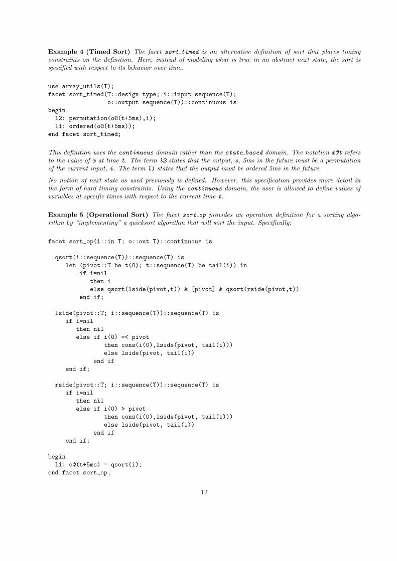
Example 4 (Timed Sort) The facet sort timed is an alternative definition of sort that places timingconstraints on the definition. Here, instead of modeling what is true in an abstract next state, the sort isspecified with respect to its behavior over time.

use array_utils(T);facet sort_timed(T::design type; i::input sequence(T);

o::output sequence(T))::continuous isbeginl2: permutation(o@(t+5ms),i);l1: ordered(o@(t+5ms));

end facet sort_timed;

This definition uses the continuous domain rather than the state based domain. The notation x@t refersto the value of x at time t. The term l2 states that the output, o, 5ms in the future must be a permutationof the current input, i. The term l1 states that the output must be ordered 5ms in the future.

No notion of next state as used previously is defined. However, this specification provides more detail inthe form of hard timing constraints. Using the continuous domain, the user is allowed to define values ofvariables at specific times with respect to the current time t.

Example 5 (Operational Sort) The facet sort op provides an operation definition for a sorting algo-rithm by “implementing” a quicksort algorithm that will sort the input. Specifically:

facet sort_op(i::in T; o::out T)::continuous is

qsort(i::sequence(T))::sequence(T) islet (pivot::T be t(0); t::sequence(T) be tail(i)) in

if i=nilthen ielse qsort(lside(pivot,t)) & [pivot] & qsort(rside(pivot,t))

end if;

lside(pivot::T; i::sequence(T))::sequence(T) isif i=nil

then nilelse if i(0) =< pivot

then cons(i(0),lside(pivot, tail(i)))else lside(pivot, tail(i))

end ifend if;

rside(pivot::T; i::sequence(T))::sequence(T) isif i=nil

then nilelse if i(0) > pivot


end ifend if;

beginl1: o@(t+5ms) = qsort(i);

end facet sort_op;

12

This specification is interesting due to its similarity to a VHDL specification and its equivalence to sort req.The sort op specification specifies that the output parameter 5ms in the future is equal to the result ofapplying quicksort to the input parameter i. The details of the application are unimportant. Suffice to saythat excluding the concept of a wait statement, this is quite similar to how a VHDL specification might bedefined.

The function qsort and the auxiliary functions lside and rside define a quicksort algorithm over sequences.The definition follows the classic recursive style. As with other function definitions in these examples, thesefunctions require some further study to understand completely. At this point it is important only to understandthat parameters to the function are specified as param-var::param-type, separated by the “;” token andenclosed within parantheses. The final expression defines the return value. In the case of lside, all valuesless than or equal to the pivot value are found recursively and returned.

A potentially cleaner specification might have the form:

package work(T::univ)::logic isexport sort_op;

begin

qsort(i::sequence(T))::sequence(T) islet (pivot::T be t(0); t::sequence(T) be tail(i)) in

if i=nilthen ielse qsort(lside(pivot,t)) & [pivot] & qsort(rside(pivot,t))

end if;

lside(pivot::T; sequence(T))::sequence(T) isif i=nil

then nilelse if i(0) =< pivot


end ifend if;

rside(pivot::T; i::sequence(T)):: sequence(T) isif i=nil

then nilelse if i(0) > pivot


end ifend if;

facet sort_op(i::input T; o::output T) isbegin continuousl1: o@(t+5ms) = qsort(i);

end facet sort_op;

end package work;

Here the function specifications are removed from the facet specification. The facet and functions are includedin the package work. The similarity to VHDL here is intentional. Unlike VHDL, the package is parameterizedallowing specialization for arbitrary types. Note the inclusion of the export sort op clause. This causes

13

the sort op facet to be visible outside the package. Other declarations such as qsort, lside and rside arehidden in the package.

Why the obsession with sort? Thus far, an axiomatic, continuous time and operational continuous timespecification have been developed. Together, we can use all three specifications to define various charac-teristics of a single sorting component in a manner unique to Rosetta. Specifically, in the next section wewill define how a designer can specify a sorting component by combining specifications from multiple do-mains. The result is a requirements specification, a temporally constrained requirements specification, anoperational specification, and a power specification simultaneously describing a system. With the additionof facet composition operators, this provides a powerful mechanism for mixing and composing specifications.

Example 6 (Alarm Clock System) Consider the following definition of an alarm clock taken from theSynopsys synthesis tutorial. This alarm clock provides a basic capability for setting time, setting alarm,sounding an alarm and keeping time. The specification states the following requirements:

1. When the setTime bit is set, the timeIn is stored as the clockTime and output as the display time.

2. When the setAlarm bit is set, the timeIn is stored as the alarmTime and output as the display time.

3. When the alarmToggle bit is set, the alarmOn bit is toggled.

4. When clockTime and alarmTime are equivalent and alarmOn is high, the alarm should be sounded.Otherwise it should not.

5. The clock increments its time value when time is not being set.

The systems level description of the alarm clock is defined in the following facet:

use timeTypes;facet alarmClockBeh(timeIn::input time; displayTime::output time;

alarm::output bit; setAlarm::input bit;setTime::input bit; alarmToggle::input bit)::state_based is

alarmTime :: time;clockTime :: time;alarmOn :: bit;

beginsetclock: setTime=1 =>

clockTime’ = timeIn and displayTime’ = timeIn;setalarm: if setAlarm=1

then alarmTime’ = timeIn and displayTime’ = timeInelse alarmTime’ = alarmTime

end if;displayClock: setTime = 0 and setAlarm = 0 =>

displayTime’ = clockTime’;tick: setTime => clockTime’ = increment_time(clockTime);armalarm: if alarmToggle = 1

then alarmOn’ = -alarmOnelse alarmOn’ = alarmOn

end if;sound: alarm’ = alarmOn and %(alarmTime=clockTime);

end facet alarmClockBeh;

14

Inputs correspond to data and control values for the clock. timeIn contains the current time input and canbe used to set either the alarm time or the clock time. displayTime is the time currently being displayed.alarm drives the audible alarm. setAlarm and setTime control whether the alarm time or clock time arecurrently being set. alarmToggle causes the alarm set state to toggle.

Local variables correspond to the state of the clock. alarmTime is the current time associated with soundingan alarm. clockTime is the current time. alarmOn is “1” when the alarm is set and “0” otherwise.

Exploring the specification indicates that each requirement is defined as a labeled term. Each term can betraced back to a requirement from the English specification. Term setclock handles the case where the clocktime is being set. Term setalarm handles when the alarm time is being set. Term armalarm handles thetoggling of the alarm set bit. tick causes the clockTime to be incremented. The clock time is incrementedin the next state only when the clock time is not being set. Finally, the sound term defines the alarm outputin terms of the alarmOn bit and whether the alarmTime and clockTime values are equal. The “%” notationtransforms the boolean result of equals into a bit value. All terms must be simultaneously true. Thus, thespecification has the same effect as using multiple processes in VHDL.

The alarm clock facet uses the following collection of time manipulation functions and types:

package timeTypes::logic isbegin

hours :: subtype(natural) is sel(x::natural | x =< 12);minutes :: subtype(natural) is sel(x::natural | x =< 59);time :: type is data record(h::hours; m::minutes)::time?;

increment_time(t:: time) :: time isrecord(increment_hours(t); increment_minutes(t));

increment_minutes(t:: time) :: minutes isif t(m) < 59

then t(m) + 1else 0

end if;

increment_hours(t::time) :: hours isif t(m) = 59

then if t(h) < 12then t(h) + 1else 1

end ifelse t(h)

end if;end package timeTypes;

hours and minutes are restricted subranges of natural number representing hours and minutes respectively.The notation type(natural) indicates that hours and minutes are bunches, not singleton values. The sel

operation provides a comprehension operator and is used to filter natural numbers. time is a constructedtype defined as a record containing an hours value and a minutes value.

Three increment functions define incrementing time. increment time forms a record from the results ofincrementing the current hours and minutes values. increment hours and increment minutes handle in-crementing hour and minute values respectively. Note that the field names are used to reference hours andminutes values respectively.

%% Remove this definition or fix it.

15

Example 7 (Stack definition) For formal specification fans, a semi-constructive stack definition is in-cluded to describe an alternate means for function specification. Here, the traditional stack operations aredeclared, but are not defined directly. The distinction with other function definitions being that no constantdefinition appears in conjunction with the declaration. Assume here that there exist in the containing packagedeclarations for EType and SType. Then the specification takes the form:

facet stack::logic ispush(E::Etype;S::Stype)::Stype;pop(S::Stype)::Stype;top(S::Stype)::Etype;is_empty(S::Stype)::boolean;empty::Stype;

beginax1:forall(e::Etype|forall(s::Stype|pop(push(e,s))=s));ax2:forall(e::Etype|forall(s::Stype|top(push(e,s))=e));ax3:forall(e::Etype|forall(s::Stype|not(is_empty(push(e,s)))));ax4:is_empty(empty);

end facet stack;

This is a canonical constructive specification for a stack. In the declarations section, push, pop, and top aredefined to operate over stacks and elements. The axioms defined as ax1 through ax4 constrain the values offunctions in the traditional declarative fashion.

This specification style may prove uncomfortable for traditional VHDL users. An alternate definition usessequences to represent the stack:

package stackAsSeq(E::type)::logic isbeginS::subtype(sequence(universal)) is sequence(E);push(s::S; e::E) :: S is cons(e,s);pop(s::S) :: S is tl(s);top(s::S) :: E is hd(s);empty::S is nil;is_empty(s::S) :: boolean is s=empty;

end package stackAsSeq;

This stack definition uses the package construct to present a series of direct definitions. No terms are neededto describe the behavior of the provided type. The stack type, S, is not an uninterpreted type but is defined asa sequence of type E. The basic stack operations are now defined on the stack type using concrete operations.

An interesting exercise is to consider the meaning of:

stack(E,sequence(E)) and stackAsSeq(E)

As we shall see later, facet composition states that properties of both stack and stackAsSeq must apply inthe facet formed by and. Effectively, this new definition is consistent only if stackAsSeq obeys the axiomaticdefinition provided by stack. In essence, stack represents requirements while stackAsSeq represents animplementation of stack.

16

Summary: A facet is the basic unit of Rosetta specification. It consists of a label, optional parameterlist, optional declarations, a domain and terms that extend its domain. Variable declaration is achievedusing the notation v::T interpreted as the value of v is contained in T. Constants are similarly definedusing the notation v::T is c interpreted as the value of v is contained in T and is equal to c. Domainsprovide a vocabulary for defining specifications. Terms extend domains to provide definitions for the specificcomponents. Terms are declarative constructs that are accompanied by a label. Any label defined in aRosetta specification may be exported and referenced using the canonical facet-name.label notation. Bydefault, all labels are exported. However, an explicit export statement may be used in the declaration sectionto selectively control label export.

2.2 Facet Aggregation

An important system level specification activity is aggregation of facets into general purpose architectures.Rosetta supports this directly using facet inclusion and facet labeling. Facet inclusion occurs when a facetname is referenced in a facet term. Facet labeling occurs when a facet is given a new label.

Consider the trivial example of defining a three input and gate from two input and gates:

facet andgate(x, y::input bit; z::output bit)::state_based isbegin state_based

l1: z’ = x and y;end facet andgate;

facet andgate3(a,b,c::input bit; d::output bit) isi:: bit;

beginl1: andgate(a,b,i);l2: andgate(i,c,d);

end facet andgate3;

The resulting definition is quite similar to structural VHDL without explicit component instantiation. Thefirst facet clearly defines the behavior of a simple and gate while the second seems to use facets as terms.The terms l1 and l2 both reference andgate and are interpreted as stating that the definitions providedby each are true. Thus, the first term instantiates andgate with items a, b and i where i is an internallydefined variable of type bit. Thus, the facet asserts that i is equal to a and b. The second term does thesame except it asserts that d is equal to i and c.

Communication between facets is achieved by sharing items. Here, the items are variable items definedeither in the parameter list or in the body of the including facet. This models instantaneous exchange ofinformation between facets via variables. Later, channels will be introduced to provide means for definingconnections with properties such as storage and delay.

Although similar to VHDL structural definition, this Rosetta definition style is semantically quite different.To understand this requires some understanding of labels and item labeling. The notation l: term definesterm and associates label l with it. Thus, the definition:

l1: andgate(a,b,i);

asserts andgate(a,b,i) as a term and associates label l1 with it. Effectively, the definition renames andgatelocally to l1. Thus, the terms l1 and l2 define facets equivalent to andgate, but with new names. Thereasoning for this is demonstrated in any definition where components that locally define variables andconstants have multiple instances. For example, consider the following incorrect specification:

17

facet register(i::in bitvector; o::out bitvector;load::in bit)::state_based is

memory::bitvector;beginload1: if %load then memory’=i else memory’=memory end if;output: o’=memory;

end facet register;

facet registerx2(i1,i2::input bitvector;o1,o2::output bitvector;load::input bit) is

begin state_basedregister(i1,o1,load);register(i2,o2,load);

end facet registerx2;

Consider the memory variable associated with each register. In the above definition, register.memoryreference to the memory variable in facet register. Unfortunately, there’s no way to learn which register.Further, because the register variables share the same name in the facet, they must be equal.

The proper definition is:

facet register(i::input bitvector; o::output bitvector;load::input bit)::state_based is

memory::bitvector;beginload1: if %load then memory’=i else memory’=memory endif;output: o’=memory;

end facet register;

facet registerx2(i1,i2::input bitvector;o1,o2::output bitvector;load::input bit)::state_based is

beginr1:register(i1,o1,load);r2:register(i2,o2,load);

end facet registerx2;

In this definition, the facet register is “copied” and relabeled twice. In the first case, the new facet is namedr1 and in the second, r2. The memory variable associated with r1 is referenced via r1.memory and similarlyfor r2.memory. Now there is no conflict and the elements of each component have unique references. Thisaspect of labeling is simple, but extraordinarily powerful.

Summary: Including facet definitions as terms supports structural definition through facet aggregation.Including and instantiating facets in definitions is achieved using relabeling. Instantiating facets replacesformal parameters with actual items. Unique naming forces these items to be shared among facets providingfor communications. When a facet is renamed, all of its internal items are renamed making each instance ofthat included facet unique.

%% The following section is way out of date given the updates to the%% facet algebra. We need to rethink facet declaration to include%% parameters (using a notation like functions) to make this happen%% correctly. I think we can use the same semantics.

18

2.3 Facet Composition

The essence of systems engineering is the assembling of heterogenous information in making design decisions.Rosetta supports this type of specification directly with operations collectively known as the facet algebra.The facet algebra provides mechanisms for defining new specifications by composing existing specificationsusing the standard operators and, or, and not.

In the context of facets, these are not logical operators. The operation F1 and F2 does not have a booleanvalue. Instead, it defines a new facet with properties from both F1 and F2. Looking ahead, this operationprovides us a mechanism for combining properties from several facets into a single facet.

Facets under composition must maintain the logical truths as specified by standard interpretations of logicalconnectives. For example, if F3 = (F1 and F2), then F3 is consistent if and only if F1 and F2 is consistent(Note: F1 and F3 are enclosed in parentheses because = has higher precedence than and). Facet compositionis useful for specifying many systems level properties by combining properties from various facets. A newfacet can be defined via composition by an expression of the following form:

<name >(<paramlist >) is <facet expression >;

where < name > is the new name, < paramlist > is an optional parameter list, and < facet expression >is an expression comprised of facet algebra operations.

The following examples describe several prototypical uses of facet composition. Please note that domainsused in these examples are defined in an accompanying document.

F1 and F2 Facet conjunction states that properties specified by terms T1 and T2 must by exhibited by thecomposition and must be mutually consistent. Further, the interface is I1 ∪ I2 implying that all symbolsvisible in F1 and F2 are visible in the composition.

The most obvious use of facet conjunction is to form descriptions through composition. Of particular in-terest is specifying components using heterogeneous models where terms do not share common semantics.A complete description might be formed by defining requirements, implementation, and constraint facetsindependently. The composition forms the complete component description where all models apply simulta-neously.

Example 8 (Requirements and Constraints) Reconsider the previously defined facets sort req andsort const. Recall that sort req defined requirements for a sorting component while sort const defined apower constraint over the same component. A sorting component can now be defined to satisfy both facets:

sort :: facet is sort_req and sort_const;

Informally, sort: (i) outputs a sorted copy of its input; and (ii) consumes only 5mW of power. Formally,the new facet sort is the product of properties from sort req and sort const. In this example, the inter-action between constraints domain and other requirements domains are unspecified. Therefore, analysis ofinteractions will reveal little additional information. However, it is certainly possible to define a relationshipbetween the constraints and state based domains if desirable.

Example 9 (Postcondition Specifications) Consider again the specifications for sort req and sort op.The first facet specifies the requirements for a sorting component using a black-box, axiomatic style. The sec-ond facet defines sorting using a specific, operational algorithm. Like the constraint model and requirementsmodels previously, sort req and sort op can be combined into a single sorting definition:

sort :: facet is sort_req and sort_op;

19

Here, the composition behaves much differently. The state-based and models do interact in interesting ways.The composition of sort req and sort op provides a pre- and post-condition for the operational sortingdefinition. The net effect is like an assertion in VHDL. However, the requirements are specified distinctlyand are not intermingled in the operational definition. Thus, for this composition to be consistent, theoperational specification must hold along with it’s real time constraints and the axiomatic specification musthold defining pre- and post-condition requirements on the composition.

Similarly, a sort specification can be developed that combines requirements, operational and constraint models:

sort :: facet is sort_req and sort_op and sort_const;

F1 or F2 Facet disjunction states that properties specified by either terms T1 or T2 must be exhibited bythe composition. Note that this is logical or, not exclusive or. The most obvious use of facet disjunction iscombining different component models into a component family. The following example illustrates such asituation.

Example 10 (Component Version) Consider the following definitions using sort facets defined previ-ously:

multisort::facet is sort_req and (bubble_sort or quicksort);

The new facet multisort describes a component that must sort, but may do so using either a bubble sort orquicksort algorithm. While and is a product operator, or is a sum operator over facets.

Other facet operations are defined and include negation, implication and equivalence. These will be presentedin detail in a later chapter. The objective here is simply to demonstrate various facet composition operationsand where they might apply in a specification.

Summary: The facet algebra supports combining facet definitions into new facet definitions. The and andor operations corresponding to product and sum operations over facets combine facets under conjunctionand disjunction respectively. The and operation defines new facets with all properties from both constituentfacets. The or operation defines new facets with properties from either facet.

2.4 Packages

Packages provide a convenient way of aggregating similar Rosetta structures including facets, types, functionsand other definitional elements. Semantically, a package is simply a facet with: (i) no terms section; and(ii) explict export of defined symbols. This, the package construct allows only the declaration of new items.The Rosetta package is intended function much like a VHDL package.

Packages are define using the package keyword and name, a parameter list, domain and definitions betweena begin-end pair. The name labels the package and provides an access mechanism. The parameter listprovides a means for defining models around a common parameter set. Only parameters of kind design areallowed. Leaving out the kind specifier causes a parameter definition to default to design. The domaindefines a base domain for all contained definitions. Definitions may include any Rosetta definitional structureincluding constants, types, functions and relations, facets and other packages.

The form of a package is shown in the following example:

20

package mathops(w:natural)::logic isbeginword::word(w);

bv2nat(w::word)::natural;nat2bv(n::natural)::word;

component adder(i1,i2::bitvector[w], o::bitvector[w+1]) isbegindefinition state-based

bv2nat(o’) = bv2nat(i1)+bv2nat(i2);end definition;end adder;

component multiplier(i1,i2::bitvector[w], o::bitvector[2*w]) isbegindefinition logic

bv2nat(o’) = bv2nat(i1)*bv2nat(i2);end definition;end multiplier;

end mathops;

By default, all symbols from the package are visible by compilation units using the package. If an exportclause is present, only listed labels are visible. Users are strongly encouraged to explicitly export symbolsfrom packages. As with facets, exported package labels are referenced using the “package.label” notation.

Packages are included in other compilation units using the use keyword and a fully instantiated packagename. To use the previous package definition contents within a second package, the following notation isused:

use mathops(8);

The result is inclusion of the facet in the immediately following compilation unit. Note that all mathopsparameters must be instantiated when it is included. The adder component in mathops is referenced usingthe notation mathops.adder unless the reference is unambiguous. In this case, simply using adder isappropriate. If a local definition of adder is declared in the including compilation unit or more than onedefinition of adder is present, then the dot notation must be used. If a facet includes multiple instances ofmathops, parameters disambiguate definitions as in mathops(8).adder.

%% Note that there are still examples remaining in the systems%% chapter that we might want to move

%% Do we want to keep the concept of interface and body compilation%% units. Entered as bug 163.

2.5 Label Visibility and Resolution

Rosetta is at its essence a statically scoped language where the declaration associated with a symbol beingreferenced in an expression can be found at compile time. When resolving a label instance, there are fivebasic sources for declarations that comprise the context: (i) the local declarative scope; (ii) the enclosing

21

compilation unit; (iii) the facet domain; (iv) packages identifed in a use clause; and (v) the context of theenclosing compilation unit.

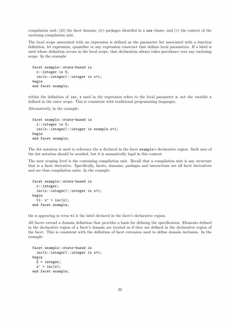
The local scope associated with an expression is defined as the parameter list associated with a functiondefinition, let expression, quantifier or any expression construct that defines local parameters. If a label isused whose definition occurs in the local scope, that declaration always takes precidence over any enclosingscope. In the example:

facet example::state-based isx::integer is 5;inc(x::integer)::integer is x+1;

beginend facet example;

within the definition of inc, x used in the expression refers to the local parameter x, not the variable xdefined in the outer scope. This is consistent with traditional programming languages.

Alternatively, in the example:

facet example::state-based isx::integer is 5;inc(x::integer)::integer is example.x+1;

beginend facet example;

The dot notation is used to reference the x declared in the facet example’s declarative region. Such uses ofthe dot notation should be avoided, but it is semantically legal in this context.

The next scoping level is the containing compilation unit. Recall that a compilation unit is any structurethat is a facet derivative. Specifically, facets, domains, packages and interactions are all facet derivativesand are thus compilation units. In the example:

facet example::state-based isx::integer;inc(x::integer)::integer is x+1;

begint1: x’ = inc(x);

end facet example;

the x appearing in term t1 is the label declared in the facet’s declarative region.

All facets extend a domain definition that provides a basis for defining the specification. Elements definedin the declarative region of a facet’s domain are treated as if they are defined in the declarative region ofthe facet. This is consistent with the definition of facet extension used to define domain inclusion. In theexample:

facet example::state-based isinc(x::integer)::integer is x+1;

beginS = integer;s’ = inc(s);

end facet example;

22

The state type S and the state variable s are defined in the domain state-based. Thus they are referencedusing their undecorated names without using the dot notation. Note state-based.s is not defined as thefacet extends the domain rather than encapsulating the domain. In the example:

facet example::state-based isS::type is integer;inc(x::integer)::integer is x+1;

begins’ = inc(s);

end facet example;

the declaration of type S represents a redeclaration error because the declaration of S in state-based istreated as a local definition. Thus, the term S = integer is used in the previous facet definition to makethe value of the state type concrete.

Packages used by a compilation unit represent the next source of scope and context information to considerwhen resolving a symbol. Three cases exist: (i) a label is declared locally and in a package; (ii) a label isdeclared in a single package; and (iii) a label is declared in multiple packages.

In the example:

package test::logic isbegin

x::integer;end package test;

use test;facet example::state-based is

inc(x::integer)::integer is x+1;begin

t1: x’ = inc(x);end facet example;

the x instance in used in the term t1 refers to the declaration in package test. It is used without the dotnotation because there is only one possible source for the declaration. In the following example, multipleused packages define x:

package test0::logic isbeginx::real;

end package test;

package test1::logic isbeginx::integer;

end package test;

use test0;use test1;facet example::state-based isinc(x::integer)::integer is x+1;

begint1: test1.x’ = inc(test1.x);

end facet example;

23

Here the dot notation must be used to eliminate ambiguity in the determination of what declaration x refersto. If a local x is defined:

package test0::logic isbegin

x::real;end package test;



use test0;use test1;facet example::state-based is

x::type is integer;inc(x::integer)::integer is x+1;

begint1: x’ = inc(test1.x);

end facet example;

then the unqualified instance refers to the local definition. Note that definitions from packages can bereferenced by explicitly using the package name.

Finally, it may be that a label is defined in the compilation unit containing facet example:

package scoping_example::logic isx::integer;


x::real;end package test;



use test0;use test1;facet example::state-based is

inc(x::integer)::integer is x+1;begin

t1: scoping_example.x’ = inc(test1.x);end facet example;

end package scoping_example;

when no local definition is present, the undecorated reference cannot be resolved to a single declaration of x asit is defined in the containing compilation unit and two packages. Thus, the package name must be explicitlyincluded in the label reference. If no declaration is present except the declaration in scoping example, thenit may be used without the dot notation. If a local declaration is present, the local definition may always bereferenced without the dot notation.

24

A rule of thumb for Rosetta scoping is that the local definition (in the facet or its domain) is always referencedwithout using the dot notation. If the local declaration is not present and only one declaration exists inthe scope of the reference, then it may be used with our without the dot notation. If multiple declarationsare present, then any declaration other than a local declaration must be referenced explicitly using the dotnotation. Any active declaration may be referenced by using it’s compilation unit name and the dot notation.

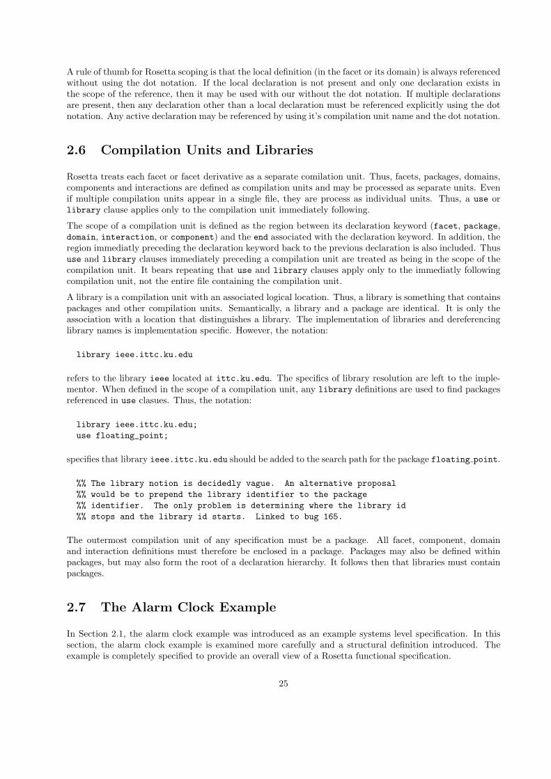
2.6 Compilation Units and Libraries

Rosetta treats each facet or facet derivative as a separate comilation unit. Thus, facets, packages, domains,components and interactions are defined as compilation units and may be processed as separate units. Evenif multiple compilation units appear in a single file, they are process as individual units. Thus, a use orlibrary clause applies only to the compilation unit immediately following.

The scope of a compilation unit is defined as the region between its declaration keyword (facet, package,domain, interaction, or component) and the end associated with the declaration keyword. In addition, theregion immediatly preceding the declaration keyword back to the previous declaration is also included. Thususe and library clauses immediately preceding a compilation unit are treated as being in the scope of thecompilation unit. It bears repeating that use and library clauses apply only to the immediatly followingcompilation unit, not the entire file containing the compilation unit.

A library is a compilation unit with an associated logical location. Thus, a library is something that containspackages and other compilation units. Semantically, a library and a package are identical. It is only theassociation with a location that distinguishes a library. The implementation of libraries and dereferencinglibrary names is implementation specific. However, the notation:

library ieee.ittc.ku.edu

refers to the library ieee located at ittc.ku.edu. The specifics of library resolution are left to the imple-mentor. When defined in the scope of a compilation unit, any library definitions are used to find packagesreferenced in use clasues. Thus, the notation:

library ieee.ittc.ku.edu;use floating_point;

specifies that library ieee.ittc.ku.edu should be added to the search path for the package floating point.

%% The library notion is decidedly vague. An alternative proposal%% would be to prepend the library identifier to the package%% identifier. The only problem is determining where the library id%% stops and the library id starts. Linked to bug 165.

The outermost compilation unit of any specification must be a package. All facet, component, domainand interaction definitions must therefore be enclosed in a package. Packages may also be defined withinpackages, but may also form the root of a declaration hierarchy. It follows then that libraries must containpackages.

2.7 The Alarm Clock Example

In Section 2.1, the alarm clock example was introduced as an example systems level specification. In thissection, the alarm clock example is examined more carefully and a structural definition introduced. Theexample is completely specified to provide an overall view of a Rosetta functional specification.

25

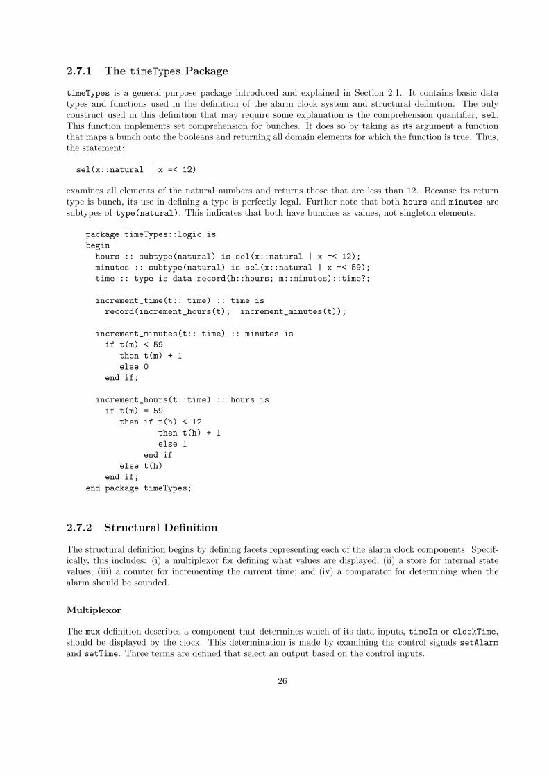
2.7.1 The timeTypes Package

timeTypes is a general purpose package introduced and explained in Section 2.1. It contains basic datatypes and functions used in the definition of the alarm clock system and structural definition. The onlyconstruct used in this definition that may require some explanation is the comprehension quantifier, sel.This function implements set comprehension for bunches. It does so by taking as its argument a functionthat maps a bunch onto the booleans and returning all domain elements for which the function is true. Thus,the statement:

sel(x::natural | x =< 12)

examines all elements of the natural numbers and returns those that are less than 12. Because its returntype is bunch, its use in defining a type is perfectly legal. Further note that both hours and minutes aresubtypes of type(natural). This indicates that both have bunches as values, not singleton elements.

package timeTypes::logic isbeginhours :: subtype(natural) is sel(x::natural | x =< 12);minutes :: subtype(natural) is sel(x::natural | x =< 59);time :: type is data record(h::hours; m::minutes)::time?;

increment_time(t:: time) :: time isrecord(increment_hours(t); increment_minutes(t));

increment_minutes(t:: time) :: minutes isif t(m) < 59

then t(m) + 1else 0

end if;

increment_hours(t::time) :: hours isif t(m) = 59

then if t(h) < 12then t(h) + 1else 1

end ifelse t(h)

end if;end package timeTypes;

2.7.2 Structural Definition

The structural definition begins by defining facets representing each of the alarm clock components. Specif-ically, this includes: (i) a multiplexor for defining what values are displayed; (ii) a store for internal statevalues; (iii) a counter for incrementing the current time; and (iv) a comparator for determining when thealarm should be sounded.

Multiplexor

The mux definition describes a component that determines which of its data inputs, timeIn or clockTime,should be displayed by the clock. This determination is made by examining the control signals setAlarmand setTime. Three terms are defined that select an output based on the control inputs.

26

// mux routes the proper value to the display output based on the// settings of the setAlarm and setTime inputs.use timeTypes;facet mux(timeIn::input time; displayTime::output time;

clockTime::input time; setAlarm::input bit;setTime::input bit)::state_based is

beginl1: %setAlarm => displayTime’ = timeIn;l2: %setTime => displayTime’ = timeIn;l3: %(-(setTime xor setAlarm)) => displayTime’ = clockTime;

end facet mux;

Recall that the Rosetta operator % converts bit values into boolean values allowing bits to be used inimplications directly.

Store

The store component is the store for the alarm clock’s internal state. It operates by examining the controlbit associated with each stored value. If the control bit is set, a new value is loaded from an appropriateinput, or in the case of alarmOn, toggling the existing value. If the associated control bit is not set, then thestored value is retained.

// store either updates the clock state or makes it invariant based// on the setAlarm and setTime inputs. Outputs are invariant if// their associated set bits are not high.use timeTypes;facet store(timeIn::input time; setAlarm::input bit; setTime::input bit;

toggleAlarm::input bit;clockTime::output time; alarmTime::output timealarmOn::output bit)::state_based is

beginl1:: if %setAlarm

then alarmTime’ = timeInelse alarmTime’ = alarmTime

end if;l2:: if %setTime

then clockTime’ = timeInelse clockTime’ = clockTime

end if;l3:: if %toggleAlarm

then alarmOn’ = -alarmOnelse alarmOn’ = alarmOn

end if;end facet store;

Counter

The counter component is the simplest component involved in the definition. It states that each time theclock is invoked, its internal time is incremented.

// counter increments the current time

27

use timeTypes;facet counter(clockTime :: inout time)::state_based isbeginl4:: clockTime’ = increment_time(clockTime);

end facet counter

Comparator

The comparator implements the guts of the alarm clock’s alarm function. It determines the appropriatevalue for the alarm output given the state of the alarm set bit and the values of the alarm time and the clocktime. If the alarm is set and the alarm time and clock time are equal, then the alarm output is enabled.Again, the % operator is used to convert a boolean value into the bit value associated with the alarm output.

// comparator decides if the alarm should be sounded based on the// setAlarm control input and if the alarmTime and clockTime are// equal.use timeTypes;facet comparator(setAlarm:: in bit; alarmTime:: in time;

clockTime:: in time; alarm:: out bit)::state_based isbeginl1: alarm = %(setAlarm and (alarmTime=clockTime)) endif

end facet comparator;


The actual structural definition instantiates each component and provides appropriate interconnections.

// The alarm clock structure is defined by assembling the components// defined previously.use timeTypes;facet alarmClockStruct(timeIn::input time; displayTime::output time;

alarm::output bit; setAlarm::input bit;setTime::input bit; alarmToggle::input bit)::state_based is

clockTime :: time;alarmTime :: time;alarmOn :: bit;

beginstore_1 : store(timeIn,setAlarm,setTime,toggleAlarm,clockTime,

alarmTime,alarmOn);counter_1 : Counter(clockTime);comparator_1 : comparator(setAlarm,alarmTime,clockTime,alarm);mux_1 : mux(timeIn,displayTime,clockTime,setAlarm,setTime);

end facet alarmClockStruct;

2.7.4 The Specification

The final specification enclosed in a Rosetta package is shown in Figure 2.1.

28

package AlarmClock::logic is

use timeTypes;

facet mux(timeIn::input time; displayTime::output time; clockTime::input time;

setAlarm::input bit; setTime::input bit)::state_based is

begin

l1: %setAlarm => displayTime’ = timeIn;

l2: %setTime => displayTime’ = timeIn;

l3: %(-(setTime xor setAlarm)) => displayTime’ = clockTime;

end facet mux;

use timeTypes;

facet store(timeIn::input time; setAlarm::input bit; setTime::input bit;

toggleAlarm::input bit; clockTime::output time;

alarmTime::output time alarmOn::output bit)::state_based is

begin

l1: alarmTime’ = if %setAlarm then timeIn else alarmTime endif;

l2: clockTime’ = if %setTime then timeIn else clockTime endif;

l3: alarmOn’ = if %toggleAlarm then -alarmOn else alarmOn endif;

end facet store;

use timeTypes;

facet counter(clockTime :: inout time)::state_based is

begin

l4:: clockTime’ = increment-time clockTime;

end facet counter

use timeTypes;

facet comparator(setAlarm:: in bit; alarmTime:: in time;

clockTime:: in time; alarm:: out bit)::state_based is

begin

l1: alarm = %(setAlarm and (alarmTime=clockTime)) endif

end facet comparator;

use timeTypes;

facet alarmClockStruct(timeIn::input time; displayTime::output time;

alarm::output bit; setAlarm::input bit;

setTime::input bit; alarmToggle::input bit)::logic is

clockTime :: time;

alarmTime :: time;

alarmOn :: bit;

begin

store_1 : store(timeIn,setAlarm,setTime,toggleAlarm,clockTime,

alarmTime,alarmOn);

counter_1 : Counter(clockTime);

comparator_1 : comparator(setAlarm,alarmTime,clockTime,alarm);

mux_1 : mux(timeIn,displayTime,clockTime,setAlarm,setTime);

end facet alarmClockStruct;

end package AlarmClock;

Figure 2.1: The complete alarm clock specification

29

Chapter 3

Items, Variables, Values and Types

%% First Evaluation Complete...

3.1 Items and Values

Rosetta’s basic semantic unit is called an item. Item structures result when Rosetta descriptions are parsedprior to manipulation. Although most users will never deal directly with items, they present an effectiveway to describe the relationships between variables, values and types.

Informally, an item consists of a label naming the item, a value the item represents, and a type from whichspecific item values must be chosen. When any structure is defined in a Rosetta specification, an item iscreated with the specified label. Variables, constants, terms, even facets themselves are items in a Rosettaspecification. When a label is referred to in a specification, it refers to the value of the item it is associatedwith. An item’s set of potential values is delineated by it’s associated type. In a legal Rosetta specification,every item’s value is an element of it’s associated type. A more complete description of items can be foundin Chapter 7.

Value items, or simply values, represent items that can be used as values for other items. There are threegeneral classes of values: (i) elements; (ii) composite items; and (iii) functions. Elemental values representprimitive, atomic values that are directly manipulated by Rosetta. Elemental values include such things asintegers, naturals, characters, bits and boolean values. Traditional programming languages refer to elementalvalues as scalar. Composite values are constructed from other values. Composite values include such thingsas sequences, sets, and facets. Function values represent operations that by definition exhibit properties ofmathematical functions. The name universal is used to refer to all values. Universal is itself a type, butrefers to the Rosetta term language.

All Rosetta types are sets where a set is simply a packaged collection of values. Functions and propertiesfor sets are defined completely in Section 3.6.1. Throughout this document, the terms set and subtype areused interchangeably to refer to a subset of a set. The term type refers to any possible set. The notationa::T is used to declare a new Rosetta item and constrain its type. Appearing in a declarative region, “a::T”declares a new item labeled a of type T. Specifically, a is a new item constrained by the type constraint ain T where T is a set. If the notation a::T appears in a non-declarative section, it serves as a mechanismfor explicitly specifying the type of an expression when type inference produces ambiguous results.

By convention, we say that v::T in a declarative region of a facet declares a variable item of type T whosevalue is an element of set T. No expression is included to constrain the value of v, thus its value is not known.Similarly, the notation v::T is c defines a constant item of type T whose value is given by the expressionc. The constraint c in T must hold for the constant declaration to be consistent. Function definition is anexception to this rule where the expression c becomes the expression associated with the function, not an

30

expression evaluated to obtain a value. This notation will be explained and used extensively in the followingsections.

3.2 Elements

By definition, elements are values that are atomic and cannot be decomposed. Element types are sets ofsuch values. Numbers such as 1, 5.32, and -32, characters such as ’a’, ’B’, and ’1’, and boolean values suchas true and false represents such atomic values. In contrast, composite values such as sequences and setsare not elemental in that each is defined by describing its contents. Element values are frequently calledscalars in traditional programming languages.

The type element is comprised of the types number, character, and any new values created by enumerationdeclarations. The element type is largely a semantic construction with no common operations over allmembers of the type other than simple equality (=) and inequality (/=) operations.

3.3 Numbers

Numeric types include standard sets of values associated with traditional number systems. Predefinednumeric types include real, integer, natural, bit, imaginary, complex and boolean and are listed in thefollowing table:

Type Format Subtype Ofcomplex 1+2*j, 3*e(̂4*j) numberreal -123.456, 123.456, 1.234e56 complexposreal 123.456, 1.234e56 realrational 123/456 realinteger 123,0,-123 rationalnatural 0,123, integerposnat 123 naturalbit 1,0 naturalimaginary j, 5*j complexboolean true, false numbernumber Any element of the above types element

Predefined operators defined over number and its subtypes include: (Assuming A and B are numbers)

%% Ordering relations moved to boolean, real, and imaginary.

Operation Format Valid ForNegation - A number

3.3.1 Complex Numbers

Complex numbers form the most basic Rosetta number. All traditional number values are subtypes ofcomplex. Traditional operations such as addition and subtraction are defined over complex numbers asanticipated. Projection functions extract real and imaginary values from complex values. re returns themagnitude of a number’s real part while im returns the magnitude of the imaginary part. For any complexvalue n expressed in the cartesian form:

n = re(n)+im(n)*j

31

The polar form may also be used. For any complex value n expressed in the polar form:

n = mag(n)*e^(arg(n)*j)

The conj operator evaluates to the complex conjugate of its complex argument. The operator mag evaluatesto the magnitude of the vector associated with a complex number in the complex plane.

Additional predefined operators defined over complex and its subtypes include: (Assuming A and B arenumbers)

Operation Format Valid ForAddition and Subtraction A+B,A-B complexMultiplication and Division A*B,A/B complexPower ,A^ B complexSquare Root sqrt(A) complexImaginary and Real im(A), re(A) complexMagnitude, Conjugate and Argument abs(A), conj(A), arg(A) complexTrig functions sin(A), cos(A), tan(A) complex

arcsin(A), arccos(A), arctan(A)sinh(A), cosh(A), tanh(A)arcsinh(A), arccosh(A), arctanh(A)

Log and exponential exp(A), log(A), log10(A), log2(A) complex

Real Numbers

The type real can be defined as the subtype of complex such that im(x)=0. Formally:

real::subtype(complex) is sel(x::complex | im(x)=0);

The additional operations min, max, floor, ceiling, round, and sgn are defined over real as well astraditional ordering relationships:

Operation Format Valid ForMinimum and Maximum A min B, A max B realFloor, Ceiling and Truncate floor(x), ceiling(x), trunc(x) realRound round(x) realSignum sgn(x) realOrdering Relations A<B,A=<B,A>B,A>=B real

min and max evaluate to the minimum and maximum value of their arguments respectively.

floor evaluates to the greatest integer number less than or equal to its argument. Conversely, ceilingevaluates to the least integer number greater than or equal to its argument. trunc always truncates it’svalue towards zero.

round evaluates to ceiling if the fractional part of its argument is greater than or equal to 0.5. Otherwise,it evaluates to floor.

sgn is defined formally as (for x 6= 0):

sgn(x::real)::integer is if -(x=0) then x / abs(x) else 1 end if;

Classical ordering relationships are provided and defined the traditional manner.

The constant values e and pi are provided as real numbers:

Constant Format Valid ForExpotential e numberPi pi real

32

Positive Real Numbers

The subtype posreal is defined as the subtype of real such that all values are greater than 0.0. Formally:

posreal::subtype(real) is sel(x::real | x > 0);

No additional operators are defined over posreal beyond those defined for real.

Imaginary Numbers

The type imaginary is the subtype of complex such that its real part is 0. Formally:

imaginary::subtype(complex) is sel(x::complex | re(x)=0);

Imaginary numbers are formed by multiplying a real number by the predefined imaginary constant j. Onecan think of this as a conversion operation from real number types to imaginary numbers. Multiplying animaginary number by the imaginary constant results in a non-imaginary value. Thus, 5*j*j is equivalent to-5 as expected.

The following operators are defined over imaginary beyond those defined for complex:

Operation Format Valid ForMinimum and Maximum A min B, A max B imaginaryOrdering Relations A<B,A=<B,A>B,A>=B imaginary

min and max evaluate to the minimum and maximum value of their arguments respectively.

Classical ordering relationships are provided and defined the traditional manner.

Rational Numbers

The type rational is the subtype of real such that each value is calculated as one integer value divided byanother. Formally:

rational::subtype(real) is sel(x::real | exists(y,z::integer | x=y/z and z/=0));

No additional operators are defined over rational beyond those defined for real.

Integer Numbers

The subtype integer is a subtype of rational such that all values are discrete. Formally:

integer::subtype(rational) is sel(x::rational | floor(x)=ceiling(x));

The additional mod, div and rem functions are defined over integer in addition to operators defined overrational. All operators are defined in the traditional fashion.

Operation Format Valid ForModulo Arithmetic x mod y integerInteger Division x div y integerInteger Remainder x rem y integer

integer is closed under +, -, *, but not under /, or trigonometric operations.

33

Natural Numbers

The subtype natural can be defined as the subtype of integer such that all values are greater than orequal to 0. Formally:

natural::subtype(integer) is sel(x::integer | x >= 0);

No additional operators are defined over natural beyond those defined for integer.

Positive Natural Numbers

The subtype posnat is defined as the subtype of natural such that all values are greater than 0. Formally:

posnat::subtype(natural) is sel(x::natural | x > 0);

No additional operators are defined over posnat beyond those defined for natural.

Bits

The subtype bit can be defined as a subtype of natural consisting of the values 0 and 1. Formally:

bit::subtype(natural) is {1,0};

Additional operators defined over bit include: (Assume the declarations x,y::bit and the definitions a=%x, and b=% y):

Operation Format Definition% % 1, % true Converts bits and boolean.Inverse not x % -aConjunction and Disjunction x and y, x or y %(a and b), %(a or b)Negated Conjunction and Disjuction x nand y, x nor y not(x and y)), not(x or y)Exclusive or and nor x xor y, x xnor y %(a xor b), %(a xnor b)

The % operation translates between bit and boolean in such a way that 1 is isomorphic with true and 0 isisomorphic with false.

It should be noted that as a subtype of natural, bit is not closed under arithmetic operations such as plusand minus.

3.3.2 Lexical Structure of Number Constants

Numeric constants are represented by a strings of digits and optional sign, decimal point, exponential andradix indicators. Specifically:

• A number may be preceded by an optional “-” operator that inverts the sign of its argument. Thenumber -123 is equivalent to negative 123.• A single decimal point may be included in a number. The number 1.23 is interpreted in the traditional

manner.• A single exponent indicator may be included in a number. The number 1.234e7 is equivalent to 1.234

times 10 to the 7th power.

34

• An optional radix may be included using the notation R\N\eE where R is the radix value (up to 16),N is a number, and E is an exponent. The radix value and the exponent value are always expressed inbase 10 while the number value is specified in the indicated radix. The number 2\10001.1001\ is thebase 2 representation of the binary real value 10001.1001. Note that “\” is not a function, but a partof the number token itself.• Imaginary numbers are formed by multiplying a real value by the complex root, j. The number 5.3*j

is interpreted in the traditional fashion.• Complex numbers are formed by adding a real number to an imaginary number or using the polar

form. The number 5+2*j is interpreted as the complex number whose real part has magnitude 5 andimaginary part has magnitude 2. The number 6*e(̂pi*j) is interpreted as the complex number whosemagnitude is 6 and whose argument is pi.

3.3.3 Boolean

The Rosetta boolean type is defined by the two element set {true,false} and is a subtype of number.Although boolean is a number type, it is not a subtype of complex or natural.

The following operators are defined over boolean beyond those defined for complex:

Operation Format Valid ForMinimum and Maximum A min B, A max B booleanOrdering Relations A<B,A=<B,A>B,A>=B booleanBit/Boolean Conversion %A booleanLogical Operations A and B, A or B, A xor B boolean

A nand B, A nor B, A xnor Bnot A

min and max evaluate to the minimum and maximum value of their arguments respectively. The maximumboolean value is true and the minimum false. Classical ordering relationships are provided and defined thetraditional manner given the definitions of true and false as maximum and minimum values respectively.

The % operator converts between boolean and bit in the classical manner.

Classical logical operations including and, or, xor, nand, nor , xnor, and not are provided. and and or aresynonyms for min and max while not is a synonym for the unary operation “-”.

When treated as numeric values, true and false follow the following equivalence and ordering rules:

Property Meaningfalse = -true false is equivalent to not true-false = true true is equivalent to not falseforall(x::number | x /= true => x < true) true is the greatest numberforall(x::number | x /= false => x > false) false is the least number

Boolean values obey ordering laws, but addition, subtraction, multiplication, division and other traditionaloperations are not defined. As numbers, true acts like positive infinity and false acts like negative infinity.Consequences of this convention are numerous and useful. They include: (i) max is semantically the same asor; (ii) min is semantically the same as and; and (iii) =< is semantically the same as implication (=>) and >=is semantically the same as implied by (<=). The same laws apply to these operations in all cases, and thedifferent signs are taken to be synonyms of each other, maintained here for the sake of historical recognition.Thus, we have the following table defining min and max over true and false:

A B A min B A max Bfalse false false falsefalse true false truetrue false false truetrue true true true

35

This is identical to the truth table defining and and or. The negation operator, -, also follows directly fromthe numeric interpretation of boolean. The greatest positive number negated is the least negative number.Thus, -true = false. As negation is its own inverse, we know that -(-x)) = x for any boolean value x.Thus, -false = true. The resulting truth table has the form:

A -Afalse truetrue false

Definitions for other logical operations follow directly. Of particular interest is the definition of implicationas:

A => B == -A or B

By definition, this is equivalent to -A max B. Again, consider the truth table generated by the definition oftrue and false as numeric values:

A B -A -A max Bfalse false true truefalse true true truetrue false false falsetrue true false true

This is semantically the same as the definition of implication. Reverse implication works similarly and thedefinition of equivalence (A=B) is consistent with the above definition. Further, when values are restricted toboolean, the following equivalences hold:

A => B == A =< BA <= B == A >= BA <= B and B <= A == A = B

It should be noted that Rosetta does not define logical equivalence, iff, separately from numerical equiva-lence. Given the mathematical definition of booleans, the normal equivalence operations are sufficient.

Example 11 (Number Constants) Examples of defining number constants, including complex, its sub-types, and boolean include:

Number Interpretation12 The standard decimal constant 12-12 The standard decimal constant −121.2 The standard decimal constant 1.21.23e4 The decimal constant 1.23 ∗ 104

1.23e-4 The decimal constant 1.23 ∗ 10−4

16\E.1F\e5 The hexadecimal constant E.1F16 ∗ 165

2\1101\e-7 The binary constant 11012 ∗ 2−7

false The boolean constant falsetrue The boolean constant true

3.4 Characters

The type character is a subtype of element and is defined as the collection of unicode values.

Given a::character, b::character, and n::natural in the range of Unicode code values, operators oncharacter include:

36

Operation Format DefinitionOrd and character ord(a), char(n) Unicode valueOrdering Relations a<b, a=<b ... ord(a)<ord(b), ord(a)=<ord(b) ...Raise and lower case uc(a), dc(a) Raise/lower case

3.4.1 ASCII Type

The type ascii is a subtype of character and is defined as the subset of characters that represent ASCIIvalues. Formally:

ascii::subtype(character) is map(char,{0,..255});

No new functions are defined on ASCII other than those defined over character values.

%% Should add other character sets besides ascii.

Lexical Structure of Character Constants

Unicode literals are expressed using the standard notation ’X’ where X is a Unicode character, ’U+XXXX’where XXXX is a 4-digit, hexadecimal number. The enclosing ticks are significant and must be included.character values that have no printable form must be specified using their Unicode hex value.

Example 12 (Character Constants) Examples of defining character constants:

Character Interpretation’U+DD01’ Unicode character associated with hex DD01

’1’ ASCII character 1

’a’ ASCII character a

%% Need some decent examples of unicode constants

3.5 Enumerations

Enumerations provide a mechanism for declaring new elemental values and types by extension. When anenumeration is declared, two semantic operations are performed on the list of value items associated withthe enumeration. First, the list of values associated with the enumeration are added to element as elementaltypes if they are not already present. Second, the list of value items is assembled into a set associated withthe construction. For example, the following notation:

enumeration(apple,orange,pear)

is semantically equivalent to adding the new value items apple, orange, and pear to element and assemblingthem into a new set. Intellectually (and semantically) the enumeration construct can be evaluated as:

enumeration(apple,orange,pear) == {apple, orange, pear}

37

The distinction between the enumeration former and the set former is that the value items comprising theenumeration need not exist before the enumeration is formed. In the example above, if apple is not a valueitem prior to generating the enumeration, then it is declared as one by the enumeration. The enumerationformer is only allowed in a declarative region and cannot be used to generate sets in terms.

Enumerations can be used to define new types using the canonical Rosetta notation:

fruit :: subtype(element) is enumeration(apple,orange,pear);

This declaration creates a new item whose supertype is element and whose value is the set containing thevalue items apple, orange, and pear. A variable defined as:

x :: fruit;

must take its value from the set {apple,orange,pear}.

Only elemental values may be included in enumeration declarations. Thus, the pair of declarations:

x :: integer;c :: enumeration( x,1,z );

is illegal because x is already defined as an integer item, and so can’t be used as a label item. Assuming thatif z has been defined, it is defined as a value item, the declaration:

c :: enumeration( 1,z );

is semantically legal. A new value item z is created in the current scope and the enumeration evaluatesto the set {1,z}. Note that having been defined as a value item by the enumeration, z cannot be used asanything else in the current scope. Upon leaving the enumeration’s scope, z is again available for use as anyitem name.

%% Move the definition of label to the meta package.

Summary: The following predefined elemental types are predefined for all Rosetta specifications:

• element — All atomic values including number, character, and value items generated by enumerationformers.

• number — Subtype of element consisting of complex and boolean values.

• complex — Subtype of number and root of the numeric type tree. Formed as the the sum of anyimaginary and any real. Thus, 7.0e2 + 2.1e4*j is complex.

• imaginary — Subtype of complex where the real part is 0. Formed by any multiple of j and a real.Thus, j is imaginary as is 5e3*j.

• real — Subtype of complex where the imaginary part is 0. Thus, 4, 4.3e2, and -4.3e2 are all real.

• posreal — Subtype of real where all values are greater than 0. Thus, 4 and 4.3e2 are both posreal.

• rational — Subtype of real where values are fractions of integers. Formed by dividing one integervalue by another. Thus, 5/4 is a rational constant.

38

• integer — Subtype of rational where values are integral numeric values. Formed when no decimalpoint or negative exponent are included in the number definition. Thus, 1, 12, 12e3 and -12e3are allinteger constants.

• natural — Subtype of integer where all values are positive or zero. Thus, 0, 5 and 12e3 are allnatural constants.

• posnat — Subtype of natural where all values are greater than zero. Thus, 5 and 12e3 are all posnatconstants.

• bit — Subtype of natural consisting of the values 0 and 1. Operations on bit elements correspondto operations on the booleans in the canonical fashion.

• boolean — Subtype of number consisting of the named values true and false. True is the greatestnumber value while false is the smallest. The boolean operators and, or and not correspond to min,max and “-” respectively.

• character — Subtype of element consisting of all unicode values. Formed using notation ’x’ wherex is either a printable character, or a four digit, hexadecimal value. Thus, ’a’, ’1’, ’U+0024’ and’U+EF37’ are character constants.

• ascii — Subtype of character consisting of all ascii values. Formed using the same notation ascharacter values. Thus, ’a’ and ’1’ are ascii values.

• enumeration values — Value items formed by use of the enumeration former. An enumerationdeclaration may add new value items to the element type. The notation enumeration(x,y,z) is usedto define three new element values and assembles them into a set that can be used as a type.

3.6 Composite Types

Composite types make complex values by combining simpler values. There are two mechanisms for struc-turing: (i) containment and (ii) indexing. Containment groups items together into collections of items. Setsand sequences are both used as containers for multiple items of the same type. Sets provide a container fora specified type that is not indexed and does not contain duplicate items. Indexing establishes a functionfrom the natural numbers (from zero to the size of the structure minus one) to the elements of the structure.Sequences effectively index sets allowing individual elements within the sequence to be accessed.

3.6.1 Sets

Rosetta sets are collections of items that exhibit properties traditionally defined in classical set theory. Inthe following, assume that S and T are sets. The first table lists functions that form sets from items or othersets:

Operation Format DefinitionFormation {1}, {1,2,3} Forms a set from a collection of itemsComprehension sel(x::T | p(x)) {x | x ∈ T and p(x)}Union S+T {x | x ∈ T ∨ x ∈ S}Intersection S*T {x | x ∈ T ∧ x ∈ S}Difference S-T {x | x ∈ S ∧ x /∈ T}Power Set set(T) (S in set(T)) == S=<TInteger Sequence {i,..j} sel(x::integer | x >= i and x =< j)Image image(f,S) f applied to each element of S

The basic set former takes an arbitrary collection of items and forms a set by extension. Each argument tothe set former is treated and evaluated as an expression. The sel operation provides a set comprehension

39

capability where one set is filtered to form another. In the table, elements of T are filtered by the booleanpredicate p to form a new set. Operations for intersection, union, and difference are defined in the classicalmanner. The set function is equivalent to the set of all subsets of its argument and is typically used to definenew set items. The sequence operation generates sets from sequences of integers. The notation {1,..4}generates the set {1,2,3,4}. Finally, the image operation takes a function and applies it to all elements ofa set. (image is synonymous with ran defined later.)

Classical relations between sets are defined and are listed in the following table:

Operation Format DefinitionEquality S = T S =< T and T =< SInequality S /= T not(S =< T) or not(T =< S)Subset S =< T, T >= S ∀x : S · x ∈ TProper Subset S < T, T > S S =< T and S /= TElement a in S a ∈ SSize # S | S |Empty Set {} ∀x : universal · not(x ∈ {}))

Equivalence is equivalence of contents. Subset and proper subset are defined in the classical manner fromelement. The in operation defines the set theoretic concept of “element of.” Size returns the cardinality ofthe set while {} names the empty set.

Defining items of a particular set type is achieved using the set type former or the power set former. Thefollowing notation defines x to be an element of the set of all possible subsets (the power set) of another setS:

x::set(S);

The declaration may intuitively be read as “x is an element of the power set S” or alternatively as “x is asubset of S.” This is in contrast to the notation:

x::S;

that defines x to be a single element of the set S.

Like any Rosetta definition, it is possible to make a set valued item constant using an is clause to associatethe item with a value. The following notation defines a set of integers that is equal to the set containing -1,0 and 1:

trivalue::set(integer) is {-1,0,1};

Similarly, set comprehension can be used to define a set value:

natural::set(integer) is sel(x::integer | x >= 0);

In both cases, the type correctness restriction requires that the specified expression be an element of thetype. In each of the above cases, the expressed value is a set of integers and is thus a legal value. Thefollowing expression:

trivalue::set(integer) is {-0.1,0.0,0.1}

Is not type correct because the specified set value is not a set of integers.

40

3.6.2 Sequences

Sequences are indexed collections of elements that combine the features of arrays and lists into a single,indexed container data structure. Sequences differ from sets in two important ways. First, they are indexedfrom 0 and allow random access of elements via their index. If s=[1,2,1] is a sequence, then s(0)=1,s(1)=2 and so forth. Second, they allow multiple instances of the same value in the container. In theexample s=[1,2,1] the value 1 appears in both the first and last position. The simplest sequence is [], theempty sequence. If S and T, are sequences, n a natural number, e an element, and I a sequence of naturalnumbers, the following operations are defined to form sequences from items or other sequences:

Operation Format DefinitionFormation [1,2,1,4] Forms a sequence containing 1,2,1,4

in the specified orderSubscription S sub I Subsequence from S

corresponding to integer sequence ICatenation S&T ConcatenationInteger Sequence [i,..j] Sequence of integers from i to jReplacement n->e|S Copy S with element n replaced by value eEmpty Sequence [] The empty sequenceHead, tail and cons head(S),tail(S),cons(h,t) cons(head(S),tail(S))==SMapping map(f,S) map(f,[s0,s1,...]==[f(s0),f(s1),...]Reduction reduce(f,S,i) f(f(f(i,s(0)),s(1)),s(2))...Filtering filter(p,S) Include only elements satisfying p.

The sequence former, [], forms sequences by extension with ordering of elements in the sequence the sameas the lexical ordering in the former.

Subscription is an extraction mechanism where elements from a sequence are extracted to form a newsequence. Give S and an integer sequence I, S sub I extracts the elements from S referenced by elementsof I and forms a new sequence. For example:

[A,B,C,D] sub [0,2,1] == [A,C,B]

The catenation operator, &, concatenates two sequences.

The notation [i,..j] forms an integer sequence from i running to j. As an example, the functions head,tail, and cons can be defined using subscription and integer sequence as follows:

head(S) = S(0)tail(S) = S sub [1,..(#S-1)]cons(x,S) = [x]&S

S(0) returns the first element in the sequence. The integer sequence former [1,..(#S-1)] forms the integersequence from 1 to the length of S minus 1. Extracting elements of S associated with 1 through #S-1 includesall elements except the first and thus defines tail in the canonical fashion.

The replace operation allows replacement of an element within a list. The notation n->e | S generates anew sequence with the element in position n replaced by e. For example:

2 -> 5 | [1,2,3,4,5] == [1,2,5,4,5]

The map and filter operators provide mechanisms for applying a function to each element of a sequenceand filtering a sequence respectively. They correspond to ran and sel for functions and sets. The operationmap(f,S) applies f to each element of S in order, generating a new sequence. Given the definition of anincrement function:

41

inc(x::natural)::natural is x+1;

then:

map(inc,[0,1,2,3]) == [1,2,3,4]

filter(p,S) applies p to each element of S generating a new sequence of only those elements satisfying p.Given the definition of a greater than zero operation:

gtz(x::integer)::boolean is x>0;

then:

filter(gtz,[0,1,2,3]) == [1,2,3]

reduce(f,S,i) applies the binary function f recursively through the sequence S. The initialization valuei is paired with S(0) to start the process. For example, the addition operator can be used to implementsummation:

reduce( + ,[1,2,3],0) == 6

The following operations define relationships between sequences and properties of sequences:

Operation Format DefinitionEquality and inequality S = T, S /= T Lexical equivalenceAccess S(n) nth element of S from 0Ordering Relations S<T, S=<T, S>=T, S>T Lexicographical orderingSize # S SizeMin and max S max T, S min T Order defined on elementsContents ~ S Set of elements from the sequence

Equal and not equal take their canonical meanings.

The ordering operations, min and max are lexicographic ordering relations. If cons(x,S)<cons(y,T), theneither x<y or x=y and S<T. Note that for any sequence, S /= [] implies that S > []. S=<T is defined as S<Tor S=T. The S min T and S max T operators return the minimum sequence of S and T and the maximumsequence respectively.

The contents of a sequence can be extracted as a set using the notation ~ A. Duplicates are removed as wellas indexing and the ordering imposed by the indexing. For example:

~[2,1,1,1] == {1,2}

To define an item of type sequence containing only elements from type B, the following notation is used:

x::sequence(B);

To define an item of type sequence, the following notation is used:

x::sequence(universal);

where x is the new item and sequence(universal) refers to the set of all possible Rosetta sequences. Thus,sequence(universal) is any sequence while sequence(B) restricts possible sequences to the elements ofB. Semantically, sequence(B) generates the set of all finite sequences created from B and thus the typecontaining all finite sequences of B.

42

Bitvectors

A special case of a sequence is the bitvector type. Formally, bitvector is defined as:

bitvector::type is sequence(bit);

Operations over bit are generalized to bitvector’s of the same length by performing each operation onsimilarly indexed bits from the two bit vectors. Assuming that op (◦) is any bit operation, the bitvector,C, result of applying the operation over arbitrary bitvector items A and B is defined by:

forall(n::{0,..(#A-1)} | C(n) = A(n) ◦ B(n))

If either A or B is longer, then the shorter bitvector is padded to the left with 0s. to achieve the end result.

In addition, the following operations are defined over items of type bitvector: (Assume A::bitvector andn::natural)

Operation Format DefinitionBitwise Logic A or B,A and B, A xor B Logical operators

A nand B, A nor B, not AConversion bv2n(A),n2bv(n) Convert between bitvectors and naturals2’s complement twos(A) Generate two’s complementShift Operations ashr(A), ashl(A), lshl(A), lshr(A) Logical and arithmetic shiftRotate rotr(A), rotl(A) Rotate right and leftPad Operations padr(A,1,n), padl(A,0,n) Pad with value to n bits.

%% Add examples for the bitwise operations

%% Add examples for direct specification of bitvectors using strings%% (or whatever we decide to use).

The operations bv2n and n2bv provide standard mechanisms for converting between binary and naturalnumbers. It is always true that bv2n(n2bv(x))=x.

The operation twos takes the two’s complement of a binary value. The lshr and lshl operations providelogical shifts right and left while ashr and ashl provide arithmetic shifts right and left. The distinctionbeing that logical shift operations shift in 0s while arithmetic shift operations shift in 1. The rotr and rotloperations provide rotation or circular shift. Note that none of the complement, shift, or rotate operationschange the length of the bit vector.

The padr and padl operations pad or catenate a bit vector. Each takes three arguments: (i) the bitvectorbeing manipulated; (ii) the pad value (1 or 0); and (iii) the resulting length. If the length value is less thanthe length of the argument vector, padr removes bits to the right and padl removes bits to the left resultingin a vector of length n. In this case, the pad value is ignored.

A special subtype of bitvector is defined to allow definition of bitvectors with specific lengths. Thewordtype type former takes a single natural number argument and generates the type containing bitvectorsof that length:

wordtype(n::integer)::set(bitvector) is sel(b::bitvector | #b = n);

The type definitions:

43

word::subtype(bitvector) is wordtype(16);byte::subtype(bitvector) is wordtype(8);nybble::subtype(bitvector) is wordtype(4);

defines new types called word, nybble and byte that consist of all bitvectors of lengths 16, 4 and 8 respec-tively. It should be noted that wordtype is simply a function that returns a set of bitvectors. Usage offunctions in this way is defined in a subsequent chapter.

Strings

A special case of a sequence is the string type. Formally, string is defined as:

string::subtype(sequence(character)) is sequence(character);

A shorthand for forming strings is the classical notation embedding a sequence of characters in quotations.Specifically:

"ABcdEF" == [’A’,’B’,’c’,’d’,’E’,’F’]

Functions defined over strings include those defined for general sequences. In particular, the notation "abc"& "def" is appropriate for concatenation of strings. It is important to note that the ordering operations forsequences provide lexicographical ordering for strings. No additional function definitions are required.

Summary: The following predefined composite types are available in a Rosetta specification:

• set — A set is a packaged collection of items that obeys basic principles of set theory. Sets are formedby extension using the set former or by comprehension using sel. The notation set(S) refers to thepower set of S. subtype is a synonym for set used in declarations. Ten notation type is a synonymfor set(universal), the power set of all possible Rosetta items.

• sequence — A sequence is an indexed collection of items. The notation sequence(S) refers to anysequence of Rosetta items formed from the elements of set S. Sequences are formed by extensionusing the sequence former or by filtering, mapping or folding sequences using reduce and map. Thedeclaration sequence(universal) refers to any indexed collection of Rosetta items.

• string — The type string is a special sequence defined as string=sequence(character).

• bitvector — The type bitvector is a special sequence defined as bitvector=sequence(bit). Op-erations from bit are defined as bitwise operations over bitvector.

• wordtype(n::integer) — The function wordtype(n::natural) is a special function that generatesthe set of bitvectors of length n.

3.7 Functions

Defining functions in Rosetta is a simple matter of defining mappings between types. Functions are extensivemappings between two different types, called the domain and range of the function. Functions are definedby defining their domain and stating an expression that transforms elements of the domain into elementsof the range. This is achieved by introducing variables of the domain type whose scope is confined to thefunction definition and defining a result expression using that variable. The domain is given by an expressionthat describes the domain type. The range is given by an expression using the variable introduced by thefunction, called the result or result function.

44

3.7.1 Direct Definition

The direct definition mechanism for defining functions is to define the function’s signature and an expressionthat relates domain values to a range value. Functions are typically defined by providing a signature and anoptional expression. The syntax:

add(x,y::natural)::natural is x+y;

In this definition, add is the function name, x,y::integer defines the domain parameters, and integer isthe return type. Together, these elements define the signature of inc as a function add that accepts twoarguments of type natural and evaluates to a value of type natural.

Following the signature, the keyword is denotes the value of the return expression, in this case x+y. Thereturn expression is a standard Rosetta expression defined over visible symbols whose type is the return type.Literally, what the function definition states is that anywhere in the defining scope add(x,y) can be replaceby x+y for any arbitrary natural values. Whenever a function appears in an expression in a fully instantiatedform, it can be replaced by the result of substituting formal parameters by actual parameters and evaluatingthe resulting expression. Specifically, if the function instantiation add(3,4) appears in an expression, itcan be replaced by the expression 3+4 and simplified to 7. Any legal expression can be encapsulated into afunction in this manner.

Like any Rosetta definition, add is an item with an associated type and value. In this case, the type ofadd is a function type defining a mapping from two naturals into the natural. The value of add is knownand is a function encapsulating the expression x+y. The specific value resulting from function evaluation isdetermined by its associated expression.

A function signature can be defined separately by specifying its arguments and return type without anexpression. The notation:

add(x,y::natural)::natural;

defines the signature of a function add that maps pairs of natural into natural. Because this add definitionhas no associated expression, it is referred to as a function signature. Allowing the definition of a signaturewithout an associated expression supports flexibility in the definition style. In this case the expressionassociated with add can be defined directly using equality or indirectly by defining properties. Functionsignatures help dramatically in reducing over-specification in definitions.

3.7.2 Anonymous Functions and Function Types

Anonymous functions, frequently called lambda functions, are defined by excluding the name and encapsu-lating the function definition in the function former <* *>. The definition:

<* (x,y::natural)::natural is x+y*>

defines an anonymous function identical to the function add above, except the anonymous function has nolabel. Such function definitions can be used as values and are evaluated in exactly the same manner asnamed functions. Specifically:

1. <* (x,y::natural)::natural is x+y *>(1,4)2. == <* ()::natural is 1+4 *> == 5

Anonymous function signatures can also be defined in a similar manner. The definition:

45

<* (x,y::natural)::natural *>

is equivalent to the function signature defined above without associating the signature with a name. We callthis a function type because it defines a collection of functions mapping pairs of natural numbers to naturalnumbers. Technically, it defines a set of functions that map two natural numbers to a third natural number.This is true because the function’s expression is left unspecified. Because the definition represents a set offunctions, it can be used as a type in formal definitions. The definition:

add::<* (x,y::natural)::natural *>

is semantically equivalent to the earlier add signature definition. The definition says that add is of type<*(x,y::natural)::natural*> or that add is a function that maps two natural numbers to a third naturalnumber. The earlier signature definition is a shorthand for this notation provided to make definitions easierto read and write.

The definition:

add::<* (x,y::natural)::natural *> is <* (x,y::natural)::natural is x+y *>

is equivalent to the first definition of add above and semantically defines the function definition shorthand.The add function is defined as a variable of type function. The declaration asserts that the add function isequivalent to the anonymous function value mapping two integers to their sum. Any function label can bereplaced by its value, if defined.

The notation <* *> is referred to as a function former because it encapsulates an expression with a collectionof local symbols to form a function. The brackets form a scope for locally defined parameters. When noparameters are present, the function former brackets can be dropped as there is no need to define parameterscope.

Rosetta provides the special type function that contains all functions definable in a specification. Statingthat f::function says that f is a function, but does not specify its domain or range values.

A function is an element of a function type if it is an element of the set of functions associated with thetype. Given a function, f

f(x::T)::R is expr;

and a function type F:

F(x::M)::N;

then f in F if the following relationship holds:

f in F == T =< M and forall(x::T | f(x) in N)

The domain of f must be a subset of the domain of F and applying f to each element of its domain mustresult in an element of F’s specified domain.

For example, given the standard definition of inc:

inc(x::integer)::integer is x+1;

inc is an element of the function type:

46

<* (x::integer)::integer *>

because it is one specific example of a function mapping integer to integer. Specifically, the domains ofthe function and function type are the same and applying inc to any integer results in an integer.

A function type is a subtype of another function type if a subset relationship holds between them. Specifically,given two function signatures defining function types:

F1(x::D1)::R1;F2(x::D2)::R2;

Then F1 =< F2 and F1::subtype(F2) if the following holds:

F1 =< F2 == D1 =< D2 and R1 =< R2;

The distinction between subtype and type inclusion is the return type of the function type is used ratherthan its range. This is because the largest possible range associated with an element of a type must be thereturn type associated with its function type.

For example, given the function types:

F1 == <*(x::real)::integer*>F2 == <*(x::integer)::integer*>

we know that F1 =< F2 because integer =< real and integer =< integer hold for the domains andreturn types respectively.

Functions defined over function types and anonymous functions include: (Assume that f and g are functionsand F and G are a function types)

Operation Format DefinitionType Equivalence F=G, F/=G F >= G and G >= G

-(F >= G) or -(G >= F)Type Containment F=<G, F<G, F>G, F>=G Subset and proper subset relationships.Containment f in F Type membership

Type containment is define as above. Proper containment, F>G occurs when F>=G and -(F=G). Type equiv-alence, F=G occurs when the types have the same elements. A function is a member of a type, f in F if itsdomain is a subset of the type’s domain and its range is a subset of the type’s return type.

3.7.3 Function Evaluation

Evaluation of Rosetta functions follows the semantics of λ-calculus and allows for both currying and partialevaluation. All Rosetta functions are evaluated in a lazy fashion. Arguments can be instantiated andfunctions evaluated in any order. Consider the following use of inc and add:

inc(add(4,5))

Rather than evaluating in the traditional style, expand the function definitions Using the canonical definitionsof inc and add results in the following anonymous function:

<* (z::natural)::natural is z+1 *>(<* (x,y::natural)::natural is x+y *>(4,5))

47

Instantiating the argument to what was the increment function results in the following definition:

<* ()::natural is <* (x,y::natural)::natural is x+y *>(4,5) + 1 *>

As the resulting function has no arguments, the outer function former can be dropped resulting in the newanonymous function:

<* (x,y::natural)::natural is x+y *>(4,5) + 1

Instantiating the x parameter of the new function by replacing the formal parameter with its associatedactual parameter results in:

<* (y::natural)::natural is 4+y *>(5) + 1

Finally, instantiating the y parameter in the same manner results in:

<* ()::natural 4+5 *> + 1

When no arguments are defined in the scope of an anonymous function, the function former can be droppedresulting in the expected result:

4+5+1 == 10

In general, the notation <* ()::T is e *> is equivalent to simply stating e.

The same result occurs regardless of the order of instantiation. The following shows a different order resultingin the same result:

1. <* (z::integer)::integer is z+1 *>(add(4,5))2. == <* ()::integer is add(4,5)+1 *>3. == <* ()::integer is <*(x,y::integer)::integer is x+y *>(4,5)+1 *>4. == <* ()::integer is <*(x::integer)::integer is x+5 *>(4) + 1 *>5. == <* (x::integer)::integer is x+5 *>(4) + 16. == <* ()::integer is 4+5 *> + 17. == 4+5+18. == 10

3.7.4 Currying, Partial Evaluation, Function Composition and Selective Union

Thus far, all Rosetta functions have been defined by using an expression in the function definition. Rosettaprovides three additional mechanisms for function construction: (i) curried functions and partial evaluation;(ii) function composition; and (iii) selective union. Partial evaluation generates new functions by substitutingvalues for some parameters and simplifying. Function composition is simply an application of functiondefinition techniques that allow a new function to be constructed from existing functions. Selective unionallows functions to be specified by extension.

48

Currying Multi-Parameter Functions

Technically, evaluation of multi-parameter function is achieved by a process based on the concept of a curriedfunction. This process provides the basis of the evaluation process used previously. All Rosetta functionscan be expressed as functions of a single argument, or curried functions. Specifically, the function:

<* (x::R;y::S)::T is exp *>

can be expressed equivalently as:

<*(x::R)::<*(y::S)::T*> is <*(y::S)::T exp *>*>

The new function is expressed is unary function over items of type R that returns another unary functionthat maps items of type S to type T. Given a function f(x::R; y::S)::T and r::R and s::S, the followingequivalence holds:

f(r,s) == f(r)(s)

Given the definition above, this equivalence generalizes to functions of arbitrarily many variables.

Consider again the definition of add defined over two integer numbers:

add(x,y::integer)::real is x+y;

Using the previous notation, add can be expressed in a curried fashion as:

add(x::integer)::<*(y::integer)::integer*> is<*(y::integer)::integer is x+y*>;

The use of x in the expression is perfectly legal as the second function definition is done in the scope of x.

The add function is now defined over a single parameter of type integer. Its return type is no longer aninteger value, but a function that maps one integer onto another. Using this notation, adding two valuesa and b is achieved using add(a)(b) - exactly the notation discussed previously.

Now consider application of the add function using the curried function approach:

1. add(1,2)2. == add(1)(2)3. == <*(x::real)::<*(y::real)::real is x+y*>*>(1)(2)4. == <*(y::real)::real is 1+y*>(2)5. == <*()::real is 1+2*>6. == 3

The function is evaluated by substituting an actual parameter for a formal parameter in first the originaladd function and then in the unary function returned by add, exactly as it was done in the previous section.

It is particularly interesting to note the following equivalence:

1. add(1)2. == <*(x::real)::<*(y::real)::real is x+y*>*>(1)3. == <*(y::real)::real is 1+y*>

This process, called currying, defines the semantics of multi-parameter functions and is the basis for allfunction evaluation.

49

Partial Evaluation

Partial evaluation is the process of taking a function and instantiating only a subset of it’s parameters. Thesemantics of partial evaluation are defined using currying as described previously. Here, only the usage andapplication of partial evaluation are discussed.

Consider the following definition of f over real numbers:

f(x::real;y::real;z::real)::real is (x+y)/z;

Application of f follows the traditional rules of substituting actual parameters for formal parameters inthe expression and substituting the expression for the function. Partial evaluation will perform the samefunction, but will not require instantiating all parameters. Consider a situation where f is applied knowingthat in all cases the value of z will be fixed at 2 to perform an average. The following syntax partiallyevaluates f and assigns the resulting function to the new function name avg:

avg(x::real;y::real)::real;

avg=f(_,_,2);

In this definition, the “ ” symbol is used as a placeholder for a parameter that will not be instantiated. Tocalculate the value of f( , ,2), we simply follow the instantiate and substitute rule:

f(_,_,2) == <*(x::real;y::real)::real is (x+y)/2*>;

The result is a 2-ary function that returns a real value. As noted, this function calculates the average of itstwo arguments. An alternate, more compact notation for the definition is:

avg::<*(x::real;y::real)::real*> is f(_,_,2);

This general approach is applicable to functions of arbitrarily many values.

Function Composition

Function composition is an application of function definition capabilities. Assume that two functions, f andg exist and that ran(g)::dom(f). We can define a new function h as the composition of f and g using thefollowing definition style:

h(x::R)::T is f(g(x));

The approach extends to other definition styles in addition to the direct definition style.

Consider the definition of inc and a function sqr defined as:

sqr(y::integer)::integer is y^2;

The definition of a function whose value is (x+ 1)2 can be defined as:

<*(z::integer)::integer is sqr(inc(z))*>

50

Expanding the definitions of sqr and inc gives the following function:

<*(z::integer)::integer is<*(y::integer)::integer is

y^2*>(<*(x::integer)::integer is x+1*>(z))*>

The only available simplification is to substitute y’s actual parameter in to the expression for sqr giving:

<*(z::integer)::integer is <* (<* (x::integer)::integer is x+1*>(z))^2 *> *>

Continuing to substitute, replacing formal parameters with actuals and eliminating function formers whenparameters are replaced gives:

1. <*(z::integer)::integer is <* (<* z+1 *>)^2 *> *>2. == <*(z::integer)::integer is <* (z+1)^2 *> *>3. == <*(z::integer)::integer is (z+1)^2 *>

The result is a new function defined over z that gives the result of composing inc and sqr.

Selective Union

Selective union of two functions f and g is defined formally as:

(f|g)(x) = if x in dom(f)then f(x)else if x in dom(g)

then g(x)end if;

end if;

Using the if construct insures that the function associated with the first including domain will be called. Inthe above example, if dom(f)=integer and dom(g)=real, then an integer value will cause f to be selectedwhile only a real value that is not an integer will cause g to be selected. If the domains are reverse, i.e.dom(f)=real and dom(g)=integer, g will never be selected because any element of integer is also in real.If the type of x is in none of the domains specified, then the result of evaluating the function is undefined.

The domain and range of (f|g) is defined as:

dom(f|g) == dom(f)+dom(g);ran(f|g) == ran(f)+ran(g);

Selective union is highly useful for implementing a form of polymorphism. An example of a function definedby selective union is the simple non zero function:

non_zero(n::number)::boolean is(<*(n::0) is true*> |<*(n::sel(x::integer | x>0))::boolean is false*> |<*(n::sel(x::integer | x<0))::boolean is false*>)

This is a rather pedestrian use of selective union and there are better definitions of the non zero function.However, it does demonstrate how domain values can be used to select from among different functiondefinitions.

51

3.7.5 The If Expression

The Rosetta if expression is a polymorphic function that supports choice between options. The syntax ofthe if expression is:

if exp1 then exp2 else exp3 end if;

where exp1 must be of type boolean while exp2 and exp3 may be of arbitrary types.

The rules for evaluating an if expression but differ from the if statement in an imperative language. Whenexp1 is true, the expression evaluates to exp2. When exp1 is false, the expression evaluates to exp3.Specifically:

if true then a else b end if == aif false then a else b end if == b

The else clause may be omitted:

if exp1 then exp2 else end if;

In this case, the if expression evaluates to exp2 if exp1 is true and is undefined otherwise. Specifically:

if true then a end if == aif false then a end if == undefined

The domain of an if expression is simply boolean while the ranges is the union of the types of exp2 andexp3.

For convenience, an elsif construct is provided to nest if statements. The notation:

if exp1 then exp2

elsif exp3 then exp4

elsif exp5 then exp6

...else expn

end if

is semantically equivalent to:

if exp1 then exp2

else if exp3 then exp4

else if exp5 then exp6

...else expn end if

end ifend if

52

3.7.6 The Case Expression

%% The case statement section is dependent on resolution of bugs 156%% and 157

The case expression supports selection from multiple options in a manner similar to using the if constructwith the elsif extension.

The general form of a case statement is:

case exp0 iss1 -> exp1 |s2 -> exp2 |s3 -> exp3 |...sn -> exprn

end case;

where s1 -sn are sets and exp0 -expn are expressions. The case statement evaluates to expk when exp0 insk holds. If this relationship is satisfied by multiple sets, the case expression evaluates to the expressionassociated with the first such set. A default case can be achieved using universal as the set expression.The equivalence check performed in most traditional languages is performed by using singleton sets. Forexample:

case x issel(x::integer | x > 0) -> false |{0} -> true |sel(x::integer | x < 0) -> false

end case;

implements a zero test on the x.

Please note that the case statement is semantically equivalent to application of a unary function definedusing selective union. Specifically:

(<*(x::sel(i::integer | x > 0))::boolean is false *> |<*(x::0)::boolean is true *> |<*(x::sel(i::integer | x < 0))::boolean is false *> )

is identical to the previous case statement.

3.7.7 The Let Expression

Function application provides Rosetta with a mechanism for defining expressions over locally defined vari-ables. An additional language construct, the let expression generalizes this providing a general purposelet construct. The Rosetta let is much like a Lisp let in that it allows definition of local variables withassigned expressions. The general form of a let expression is:

let (x::T be ex1 ) in ex2 end let;

53

This expression defines a local variable x of type T and associates expression ex1 with it. The expressionex2 is an arbitrary expression that references the variable x. Each reference to x is replaced by ex1 in theexpression when evaluated. The be keyword is semantically similar to is. The distinction is that is clausesare evaluated when their associated variable declarations are evaluated. be clauses are evaluated when thelet form is evaluated. Unlike traditional variable declarations, let parameter definitions may not omit thebe clause. All let parameters must have values when the let form is interpreted.

The syntax of the let expression is defined by transforming the expression into a function application.Specifically, the semantic equivalent of the previous let expression is:

<*(x::T)::universal is ex2*>(ex1)

When the function is applied, all occurrences of x in ex2 are replaced by ex1. This process is identical tothe application of any arbitrary function to an expression. Assume the declaration i::integer and considerthe following let expression:

let (x::integer be i+1) in i’=x end let;

The semantics of this let expression is:

<*(x::integer)::universal is i’=x*>(i+1)

Evaluation of the function application gives:

i’=i+1

The usefulness of let becomes apparent when an expression is used repeatedly in a specification. Considera facet with many terms that reference the same expression. The let construct dramatically simplifies sucha specification.

Let expressions may be nested in the traditional fashion. In the following specification, the variable x oftype T has the associated expression ex1 while y of type R has the expression ex2. Both may be referencedin the expression ex3.

let (x::T be ex1 ) inlet (y::R be ex2 ) in ex3 end let

end let;

This expression may also be written as:

let (x::T be ex1, y::R be ex2) in ex3 end let;

The semantics of this definition are obtained by applying the previously defined semantics of let:

<* (x::T)::universal is <*(y::R)::universal is ex3 *>*>(ex1 )(ex2 )

Consider the following specification assuming that i is of type integer and fcn is a two argument functionthat returns an integer:

let (x::integer be i+1, y::integer be i+2) in i’=fnc(x,y) end let;

54

When evaluated, the following function results:

<*(x::integer)::universal is <*(y::integer)::universal is i’=fnc(x,y)*>*>(i+1)(i+2)

The result of evaluating this function is:

<*(x::integer)::universal is <*y::integer is i’=fnc(x,y)*>*>(i+1)(i+2) ==<*(y::integer)::universal is i’=fnc(i+1,y)*>(i+2) ==i’=fnc(i+1,i+2)

In order for normal argument substitution to work, the expressions in the Rosetta let expression must notbe mutually recursive. If recursion is necessary, the expressions must be represented as normal Rosetta rulesor predicates.

Summary: A Rosetta function is defined by specifying a domain, range and an expression defining arelationship between domain and range elements. The notation:

f(d::domain )::range is exp ;

Defines a function mapping domain to range where exp is an expression defined over domain parametersand gives a value for the associated range element. The notation:

f(d::domain )::range ;

defines f as an element of the set of all functions relating domain to range without specifying the precisemapping function.

As an example, the increment function is defined over naturals using the notation:

inc(x::natural)::natural is x+1;

Applying a function is simply substitution of an actual parameter for a formal parameter. Evaluating inc(2)involves replacing x with 2 and applying the definition of a function. Specifically:

inc(2) = 2+1 =inc(2) = 3

Function types are specified as anonymous functions using the notation:

<*(d::domain )::range *>

This function type specifies the set of all functions mapping domain to range. The definition:

f::<*(d::domain )::range *>

says that f is a function that maps domain to range. The function former (<* *>) defines the scope of thenamed parameter x and forms a function constant in the same manner as {} forms a set and [] forms asequence.

An anonymous function is a function having no assigned label. It is treated like a lambda function in Lispprogramming languages in that it can be evaluated like any other function, but has no name by which toreference it.

55

<*(d::domain )::range is exp *>

This anonymous function specifies the function mapping domain to range using the expression exp. It issemantically the same as f(d::domain)::range. The definition:

f::<*(d::domain )::range is exp *>

says that f is a function that maps domain to range using the expression exp. It is semantically the sameas f(d::domain)::range is exp.

The let expression provides a mechanism for defining local variables and assigning expressions to them. Thisprovides shorthand notations that can dramatically simplify complex specifications by reusing specificationfragments. The syntax of the general let expression is:

let (v1::T1 be e1, v2::T2 be e2, ..., vn::Tn be en) in exp end let;

where v1 through vn define variables, T1 through Tn define the types associated with each variable, and e1through en define expressions for each variable.

Evaluating the let expression results in the expression exp with each variable replaced by its associatedexpression. The semantics of the let expression are defined using function semantics. It is sufficient torealize that the let provides local definitions for expressions.

The if expression provides a simple mechanism for expressing choice. The general form:

if expression then cond1 else cond2 end if;

evaluates to cond1 if expression evaluates to true and cond2 if expression evaluates to false.

The case expression provides a general purpose selection method used to choose from more that two,potentially non-exclusive options. The form of the case statement is:

The general form of a case statement is:

case exp0 iss1 -> exp1 |s2 -> exp2 |s3 -> exp3 |...sn -> expn |otherwise -> exp

end case;

where expk are expressions and sk are sets or expressions that result in sets. The case expression evaluatesto the first expk such that exp0 in sk. The term otherwise is a synonym for universal and provides adefault case. If the match condition holds for none of the case terms and an otherwise term is not included,the case statement is undefined.

%% Stop First Evaluation Complete...

%% Start Evaluation Here...

56

3.8 Set Construction and Quantification

In Rosetta, all quantifiers are functions defined over other functions. A number of second order functionssuch as min and max are defined and will be presented here. Given that F(x::universal)::universal andP(x::universal)::boolean, the following quantifier and set constructor functions are defined:

Operation Format DefinitionFunction Former <* (rank)::return is exp *> Forms a function value or type.Domain dom(F) Function’s actual domainReturn Type ret(F) Signature’s return typeRange ran(F) Function’s Range or ImageMaximum and Minimum max(F),min(F) Maximum and minimum value in rangeSelection sel(P) Set ComprehensionExists exists(P) Existential quantifierForall forall(P) Universal quantifierSummation and Product +B, *B Summation and Product

%% The unary versions of + and * are being considered for removal in%% bug 166.

The signature for the min function is:

min(f::<*(x::universal)::universal*>)::universal

The min function accepts an arbitrary function and returns the minimum value associated with the rangeof the argument function. Recall that the range of the argument function is the result expression applied toeach element of the domain. Consider the following function application:

min(<*(x::{1,2,3,4})::natural is x*2 *>)

The domain of the argument is the set {1,2,3,4}. Although it is unusual to define a set by extension inthese circumstances, it is perfectly legal. The range of the argument function is the expression applied toeach element of the domain. Specifically, {2,4,6,8}. The min function then returns the minimum value in{2,4,6,8} or 2.

If the unaltered minimum value associated with the input set is desired, the min function can be appliedusing an identity function as in:

min(<*(x::{1,2,3,5})::natural is x *>)

The max function is defined similarly and operates in the same manner.

3.8.1 Domain, Range and Return Type

The ret function takes a function and returns its defined return type. This is the type specified in the functiondefinition following parameters and limits the values that can be returned by the function definition. Theran function is similar to a set mapping function and returns the image of a function with respect to itsdomain. It returns the set resulting from applying the parameter function’s expression to each element ofthe domain. By definition, ran(F) in ret(F), but it is not necessary for the range of a function to be equalto its return type. Consider the following example where ran is used to add one to each element of set B:

ran(<*(x::B)::natural is x+1*>)

57

Given that B={1,2,3}, the expression above evaluates to {2,3,4}. This is precisely the application of x+1to each element of the range set. Applying ret to the same function would return natural as the returntype.

The dom function is defined similarly to the range function but instead returns the domain associated withits function argument. For example:

dom(<*(x::T)::natural is x+1*>)

evaluates to the set T.

The domain and range functions present a greater challenge when dealing with functions of arity other than1. The domain of a nullary function is defined as the null type while the range of a nullary function is theresult of its evaluation:

dom(<* ()::natural is 3+2 *>) == nullran(<* ()::natural is 3+2 *>) == 5

Using this identity, one can define evaluation of a fully instantiated function as taking the range of thatfunction. Specifically, if all arguments to a function are known, then the range of that instantiated functionis the same as evaluating the function.

Currying is applied when looking at the domain and range of functions with arity greater than one. Recallthat any n-ary function can be treated as application of a series of unary functions. Thus, the domain offunctions with arity greater than one is defined as the type of the first parameter. Thus, for the add functiondefined by:

add(x,y::natural)::natural is x+y;

The value of dom(add) is defined as:

dom(add) == natural;

or the set of values the curried form of add can be applied to.

The range of such a function is the set of functions that result from currying over all possible domain values.Literally, it is the set of values, albeit function values, that result from applying the curried function formto the domain values. Thus for the add function:

ran(add) == image(add,natural);

the range is defined as the set of functions that result from applying add to every domain element. Theelements of the resulting set are functions of the form:

f(x::natural)::natural is x+n

where n is any natural.

The return type is defined in the same manner as for unary functions. It is the type used to define thefunction signature in its declaration. Thus, for add:

ret(add) == natural

It is important to note that the range and return type of a function are two different concepts. ran(f) is afunction of f and its application across its domain. ret(f) is associated with the signature of f and neednot be equal to its domain.

58

3.8.2 Quantifiers

As previously defined, the functions min and max provide minimum and maximum functions over functionranges. Over boolean valued functions, min and max provide quantification functions forall and exists. Asnoted earlier, and and or correspond to the binary relations min and max respectively. As forall and existsare commonly viewed as general purpose and and or operations, forall and exists should correspond tomin and max.

Consider the following application of forall to determine if a set, S, contains only integers greater thanzero:

forall(<* (x::S)::boolean is x>0 *>)

Here, the domain of the argument function is the set S and the result expression x>0. To determine therange of the argument function, x>0 is applied to each element of S. Assume that S={1,2,3}. Substitutinginto the above expression results in:

forall(<*(x::{1,2,3})::boolean is x>0 *>)

Applying the result expression to each element of the domain, the range of the function becomes:

{true,true,true} == {true}

As true is greater or equal to all boolean values, the minimum resulting value is true as expected. AssumingS={-1,0,1} demonstrates the opposite effect. Here, the range of the internal function becomes:

{false,false,true} == {false,true}

As false is less than true, the minimum resulting value is false. Again, this is as expected.

3.8.3 Selection

The function sel provides a comprehension operator over boolean functions. The signature for sel is definedas follows:

sel(<*(x::universal)::boolean*> is set(universal)*>)

Like min and max, sel observes the range of the input function. However, instead of returning a singlevalue, sel returns a set of values from the domain that satisfy the result expression. Consider the followingexample where sel is used to filter out all elements of S that are not greater than 0:

sel(<*(x::S)::boolean is x>0*>)

Assuming S={1,2,3}, x>0 is true for each element. Thus, the above application of comprehension returns{1,2,3}. If S={-1,0,1} then x>0 holds only for 1 and the instance of sel evaluates to {1}.

%% A select one operation, selone, is being discussed in bug 169

59

3.8.4 Shorthand Notation

A shorthand notation is provided to make specifying forall, exists, sel, min and max expressions simpler.Notationally, the following statement:

forall(x::S | x>0);

is equivalent to:

forall(<*(x::S)::boolean is x>0*>);

and returns true if every x selected from S is greater than 0. The notation allows specification of the domainon the left side of the bar and the expression on the right. The domain of the expression is assumed to beboolean for forall, exits, and sel. For min and max, the domain is taken from the expression. Thisnotation is substantially clearer and easier to read than the pure functional notation. Note that the originalnotation is still valid for specifying quantified functions.

The notation extends to n-ary functions by allowing parameter lists to appear before the “|” to representparameter lists. The format of these lists is identical to the format of function parameter lists. Specificexamples include:

forall(x,y::integer | x+y>0)exists(x,y::integer | x+y>0)sel(x,y::integer | x+y>0)

It is important to remember that like forall and exists, sel observes the function range and selectsappropriately. Interpreting the notation in the standard way results in the definitions:

forall(<* (x,y:integer)::boolean is x+y>0 *>)exists(<* (x,y:integer)::boolean is x+y>0 *>)sel(<* (x,y:integer)::boolean is x+y>0 *>)

%% Need to update summary section

Summary: Quantifier functions operate on other functions. Each generates the range of their functionargument and returns a specific value associated with that range. min and max return the minimum andmaximum range values respectively and are synonymous with forall and exists. sel and ran providecomprehension and image functions respectively. sel applies a specific boolean expression to a function’srange and returns a set of domain elements satisfying the expression. dom returns the domain of a functiondefined as the application of the result expression to every domain element.

3.8.5 Function Containment

Function containment, f1 =< f2, holds when a function is fully contained in another function. Assumingf1(x::d1)::r1 and f2(x::d2)::r2 where d1, d2, r1 and r2 are types representing domain and rangerespectively:

f1 =< f2 == d1 =< d2 and forall(x::d1 | f1(x) = f2(x))

60

f1 is contained in f2 if and only if the domain of f1 is contained in the domain of f2 and for every elementof f1’s domain, f1(x) is equal to f2(x).

Consider the case of determining if increment is contained in identity over natural numbers. In this case,the law should not hold:

1. inc =< id2. == <*(x::natural)::natural is x+1*> =< <*(x::natural)::natural is x*>3. == dom(inc) >= dom(id) and forall(x::natural | inc(x) = id(x))4. == natural in natural and forall(x::natural | x+1 = x)5. == true and false

false is obtained from the second expression by the counter example provided by x=0 as 0+1 /= 0.

Assume that f(x::df)::rf and g(x::dg)::rg are functions. The following operations are defined over twofunctions:

Operation Format DefinitionEquivalence f=g, f/=g f=<g and g=<f, -(f=<g) or -(g=<f)Containment f=<g, g>=f dom(f)=<dom(g) and forall(x::dom(f) | f(x)=g(x)Proper Containment f<g, g>f f >= g and f /= g

Functional equivalence checks to determine if every application of f and g to elements from the union oftheir domains results in the same value. Specifically, f(x) = g(x) for every x in either domain. Functioninequality is defined as the negation of function equality.

Function containment, f=<g, occurs when dom(f)<dom(g) and forall(x::dom(f) | f(x) = g(x). Propercontainment occur when simple containment holds and the functions are not equal.

%% Working here...

%% Consider moving this section. Technically, these are second%% order funtions, but they are specific to real and complex valued%% fuctions. Don’t know where to move them though...

3.8.6 Limits, Derivatives and Integrals

A special class of functions for defining limits, derivatives and integrals are provided for use with real valuedfunctions. These functions exist primarily to allow specification of differential equations (both ordinary andpartial) over real valued functions. Given a real valued function f(x::real)::real, the following definitionsare provided:

Operation Format DefinitionLimit lim(f,x,n) limx→n f(x)Derivative deriv(f,x) df

dxIndefinite Integral antideriv(f,x,c)

∫f(x)dx+ c

Definite Integral integ(f,x,u,l)∫ ulf(x)dx

The derivative of a function is defined with using limit in the canonical fashion. The following axiom isdefined for all real valued functions and real valued nonzero delta:

deriv(f,x) = lim((f(x+delta)-f(x))/(x+delta)-x,delta,0)

In the derivative function, f is the object function and x is the label of the parameter subject to the derivative.In the above function, the following holds:

61

deriv(f,x) = dfdx

The derivative function is generalizable to expressing partial derivatives. Assuming that g is defined overmultiple parameters, such as g(x::real;y::real;z::real)::real, then:

deriv(g,x) = ∂g∂x

Antiderivative, or indefinite integral, is the inverse of derivative. The antiderivative of f with respect to x isexpressed as:

antideriv(f,x,c) =∫

f(x)dx + c

f being the function in question, x being the variable integrated over, and c being the constant of integration.

As antiderivative is the dual of derivative, the following axiom is defined for all real valued functions:

antideriv(deriv(f,x),x,0) == deriv(antideriv(f,x,0),x) == f

The definite integral of f with respect to x over the range u to l is expressed as:

integ(f,x,l,u) ==∫ ulf(x)dx

The definite integral is defined as the difference of the indefinite integral applied at the upper and lowerbounds:

integ(f,x,l,u) == antideriv(f,x,0)(u) - antideriv(f,x,0)(l)

It is possible to express a definite integral over an infinite range using the notation:

integ(f,x,false,true) =∫∞−∞ f(x)dx

It should be noted that limit, derivative, antiderivative and integral functions are defined over real valuedfunctions only. Further, the functions provide a mechanism for expressing these operations and some semanticbasis for them. Solution mechanisms are not provided.

3.9 Universal Type

The type universal is now introduced as the supertype of all Rosetta types. This includes element, set,sequence, constructed types, function and facet types. Declaring:

x :: universal;

results in an item x that can literally contain any Rosetta value. Declaring:

f(x::universal)::universal;

results in a function f that can accept any Rosetta value and may result in any Rosetta value. Declaring:

t :: subtype(universal);

results in a type variable, t, whose value may be any set of Rosetta values.

62

3.10 User Defined Types

3.10.1 Sets and Types

As noted earlier, all Rosetta types are sets and any Rosetta set can be used as a type. To support clarity inspecifications, several notational shorthands are provided to support defining types and subtypes. The itemdeclaration notation:

i::integer;

defines an item named i whose value is restricted to single elements from the set integer. When integeris viewed as a set, this restriction can be represented as:

i in integer;

Similarly, the notation:

natural::set(integer);

implies that natural is a set of elements from integer. This constraint can be expressed using in byequating set(integer) power set of integers:

natural in set(integer);

the set natural is contained in the power set of integers and is a subset of integer. The value of naturalcan be restricted to a single element of the power set that appropriately defines naturals using the notation:

natural::set(integer) is sel(x::integer | x >= 0);

Now the set natural is constrained to be equal to the set of elements from integer that are greater thanor equal to 0. Because the expression defines a set value by comprehension over integer, we know that theexpression is contained in set(integer).

In Rosetta, sets are first class items and any set can be used as a type. Thus, natural from the previousdeclaration can be used as a type in subsequent declarations. Thus, the declaration:

n::natural;

declares a new item named n that is an element of the set natural used as a type.

Subtype and Type

In Rosetta, one type is a subtype of another if all its elements are contained in the second type. Specifically,S is a subtype of T if S=<T holds. When defining a new set using the notation:

natural::set(integer);

it is known that natural is a subset of integer and thus that natural is a subtype of integer. Thus,Rosetta provides an operation, subtype that is semantically equivalent to set:

63

natural::subtype(integer);

The subtype notation is equivalent to the set notation. Both define a new set that includes possible subsetsof integer. The subtype notation is simply syntactic sugar that provides a mechanism that a set will beused as a type.

It is also possible to define a new type that is not explicitly defined as a subtype of any existing type. Usingthe set notation, such a type is defined as:

T::set(universal);

or alternatively using subtype:

T::subtype(universal);

Both notations define a new set, T, whose elements are simply Rosetta items. No other type restriction ismade. Such sets are frequently used when defining abstract types whose construction is not specified orknown. Thus, Rosetta provides a keyword type that is equivalent to the definition subtype(universal).Specifically:

T::type;

is equivalent to the previous notations and defines a new type that has no subtype relationships with othertypes.

Both subtype and type definitions can be used to define constants in a manner identical to that for anyother Rosetta item. The is clause is included to provide a constant value for the symbol. The type naturalis defined using this technique:

natural :: subtype(integer) is sel(n::integer | n >= 0);

The following example defines a type that includes sets of exactly four integers:

set4 :: subtype(set(integer)) is sel(x::set(integer | #x=4));

where set4 is the set of subsets of integer that contain exactly four elements. In this case, set4 is a setof integer sets, not simply a set of integers. Thus, the set operation is used to generate the power set andthe new type set4 is chosen from the power set of the power set. In other words, it is itself a set of integersets. The sel operation uses the cardinality operator to choose integer subsets that contain 4 element setsonly. The notation z::set4 declares z to be an element of set4, or simply a subset of integer containingfour elements.

The type notation can be used similarly to define the natural numbers:

natural::type is sel(x::integer | x >= 0)

Using this definition, natural is still a subset of integer and is thus a subtype of integer. However, thisinformation must be inferred rather than directly found in the definition. The type declaration should beused carefully and only when defining or types not defined by filtering existing sets. If a subtype relationshipexists, then it should be specified explicitly in the definition. Even if the type’s value is not known, expressinga subtype relationship in the type definition aids automated analysis and readability.

In addition to constructing new types comprised of elements, the subtype construct can be used to definetypes comprised of composite values. The following definition:

bv::subtype(sequence(bit));

defines a new type named bv that is comprised of bitvectors. Similarly, it is possible to define types containingsets and constructed types.

64

3.10.2 Parameterized Type Formers

Any function returning a set can be used to define a Rosetta parameterized type. Consider the followingfunction definition:

word(n::natural)::subtype(bitvector) issel(b::bitvector | $b = n);

Remembering that subtype is a synonym for set, the function signature defines a mapping from naturalnumbers to a set of bitvectors. That set of bitvectors is defined by the sel operations to be those whoselengths are equal to the parameter n. Thus, word will return the set of bitvectors of length equal to itsparameter. We can now use wordtype as as a type definition construct.

The notation:

reg::word(8);

defines reg to be a bitvector of length 8.

The notation:

bv8::subtype(bitvector) is word(8);

defines bv8 to be the set of all bitvectors of length 8.

%% Summary section needs to be updated.

Summary: User defined types are declared exactly as are other Rosetta variables and constants. Whilethe notation x::T forces x to be a singleton element of T, the notation x::subtype(T) allows x to be asubset for T. Types can be formed from any element or composite type.

Uninterpreted types are defined as subtypes of the universal type.

Parameterized types are defined by using functions to return set as types.

%% Stop Evaluation Here... (Skip Forward)

3.11 Constructed Types

%% Working to determine if the type parameters from the function%% should also be expressed as parameters to the data declaration.

3.11.1 Defining Constructed Types

Rosetta provides a general shorthand for defining types in a constructive fashion. Constructor, observer andrecognizer functions are defined for the type and encapsulated in a single notation. These types are calledconstructed types and are created with the special data keyword and notation. As an example, consider adefinition for a binary tree of integers:

65

Tree(a::type) :: type is data(a::type)null::nullp |node(L::Tree(a),v::a,R::Tree(a))::nodep;

This definition provides two constructors for Tree: (i) the nullary function null; and (ii) the ternary functionnode. The null function creates an empty tree while the node function creates a node from a value and aleft and right subtree. A tree of integers can be defined as:

IntTree :: Tree(integer);

A tree with one node whose value is 0 can be generated with the following function instantiation:

node(null(),0,null());

A balanced tree with 0 as the root and 1 and 2 as the left and right nodes respectively can be generated:

node(node(null(),1,null()),0,node(null(),2,null()));

The recognizers nullp and nodep indicate the constructor used to generate a tree. Specifically, nullp istrue if its argument is null() and nodep is true if its argument is an instantiation of the node function.Semantically, these functions are defined as follows:

nullp(x::tree(integer))::boolean is x=null();

nodep(x::tree(integer))::boolean isexists(lt::tree(integer), v::integer, rt::tree(integer) | node(lt,v,rt)=x);

Finally, parameter names are used to generate observer functions that return actual parameters from con-structor functions. Specifically, the following functions are generated from the integer tree definition:

lt(t::sel(x::tree(integer) | nodep(x)))::tree(integer)rt(t::sel(x::tree(integer) | nodep(x)))::tree(integer)v(t::sel(x::tree(integer) | nodep(x)))::integer

These functions return the actual parameter instantiation of their associated formal parameter. For example:

lt(node(null(),1,node(null(),2,null()))) == null()v(node(null(),1,node(null(),2,null()))) == 1v(rt(node(null(),1,node(null(),2,null())))) = 2

The syntax for creating unparameterized constructed type definitions is:

T :: type is dataf1(b11::T11,b12::T12 ... b1i::T1i)::r1 |f2(b21::T21,b22::T22 ... b2j::T2j)::r2 |...fn(bn1::Tn1,bn2::Tn2 ... bnm::Tnm)::rn;

66

This data type definition defines n functions that create and recognize all elements of type T. Instantiatingany of the fk functions creates an element of type T. This set of functions are refered to as constructors ofthe type T.

Associated with each constructor, fk, is a boolean recognizer function rk that is true when its argument wascreated with the associated constructor function. Specifically, rk will return true when its argument wascreated using fk:

r(k)(t1, t2, t3,..., ti)==true;

Associated with each constructor function parameter is an observer function of the same name that observesthe parameter. Given an instantiated constructor function, the observer associated with a parameter willreturn the actual parameter instantiating it:

b(k)(t1, t2, t3,..., ti)==tk;

Like any other function, constructor functions can be partially evaluated. If this is the case, then the resultsof applying observer functions associated with uninstantiated parameters are not defined.

The general expression above is equivalent to the following definitions and laws (where the definitions are inthe definition section and the laws in the predicate section):

T :: type;f1(b11::T11, b12::T12 ... b1i::T1i)::T;f2(b21::T21, b22::T22 ... b2j::T2j)::T;...fn(bn1::Tn1, bn2::Tn2 ... bni::Tni)::T;

r1(t::T)::boolean is exists(b11::T11, b12::T12 ... b1i::T1i |f1(b11, b12 ... b1i)=t)

r2(t::T)::boolean is exists(b21::T21, b22::T22 ... b2j::T2j |f2(b21, b22 ... b2j)=t)

...rn(t::T)::boolean is exists(bn1::Tn1, bn2::Tn2 ... bni::Tnk |

fn(bn1, bn2 ... bni)=t)rn(t::T)::boolean is exists(bn1::Tn1, bn2::Tn2 ... bnm::Tnm |

fn(bn1, bn2 ... bnm)=t)

b11(t::f1(x,_,_ ... _))::T11 is x;b12(t::f2(_,x,_ ... _))::T12 is x;...

begint1: forall(x::T | exists(x1::b11,...,xi::b1i | f1(x1,x2, ... xi) = x) or

exists(x1::b21,...,x2::b2j | f2(x1,x2, ... xi) = x) or...exists(xn::bn1,...,xn::bnm | fn(x1,x2, ... xi) = x) or

The syntax for creating parameterized constructed type definitions adds a collection of type parameters tothe definition:

F(p1::type,...,pn::type):: type is data (p1::type,...,pn::type)f1(b11::T11, b12::T12 ... b1i::T1i)::r1 |

67

f2(b21::T21, b22::T22 ... b2j::T2j)::r2 |...fn(bn1::Tn1, bn2::Tn2 ... bnk::Tnk)::rn ;

In this case, the result is a type definition function that can be used to create new subtypes of the newtype F. Specifically, when instantiated F(p1,...pn) creates a new constructed type with constructed typevariables instantiated.

The tree example is one such parameterized constructed type definition. The new type, Tree(a), is param-eterized over a single value that is used as a type in subsequent definitions:

Tree(a::type) :: type is data(a::type)null::nullp |node(L::Tree(a),v::a,R::Tree(a))::nodep;

Thus, the definition:

IntTree :: type is Tree(integer);

This definition creates a new type called IntTree that is formed by instantiating the Tree constructed typewith integers. Alternatively:

AnIntTree :: Tree(integer);

creates a single new integer tree named AnIntTree that is of the type created by the parameterized con-structed type instantiation.

3.11.2 Records

In Rosetta, no special syntax for defining records is defined as record structures follow directly from con-structed types. A record type is a constructed type with a single constructor function that associates valueswith parameters used as field names. A typical record type will be defined with the following constructivetechnique:

record::type is datarecordFormer(f0::T0 | f1::T1 | ... fn::Tn)::recordp;

where recordFormer is the single constructor, f1through fn are the names of the various fields and T1through Tn are the types associated with those fields. The recognizer recordp is also defined, but is largelyunused. To define a specific record type that represents Cartesian coordinates, the following notation is used:

cartesian::type is datacartFormer(x::real, y::real, z::real)::cartp;

To define an item of this type, the standard Rosetta declaration syntax is used:

c :: cartesian;

Values an be associated with record items using the canonical is form:

68

origin :: cartesian is cartFormer(0,0,0);

Accessing individual fields of the record is achieved by applying one of the observer functions associated witha field name. To access field y in the record c, the following notation is used:

y(c)

Forming a record is achieved by calling the constructor function:

recordFormer(v1,v2,...,vn)

where v1 through vn name the specific values for fields f1 through fn. Defining a coordinate in Cartesianspace using the definition above is achieved by:

cartFormer(1,0,0);

Accessing the result is achieved using the observer functions:

x(cartFormer(1,0,0))==1;y(cartFormer(1,0,0))==0;z(cartFormer(1,0,0))==0;

Using the “ ” notation, it is possible to create records whose specific field values are not known. The followingcreates a cartesian coordinate whose x and y values are known, but whose z value is not specified:

cartFormer(1,0,_);

Should the function z be instantiated with this record, the return value is undefined.

%% Working here...

3.11.3 Pattern Matching

Pattern matching in parameter lists dramatically simplifies defining observer functions over type constructors.Parameter matching takes advantage of the mechanism used to create its input parameters. Consider theinteger tree definition presented above. Two constructor functions, null and node are defined to constructtwo different types of trees. Viewed differently, they also partition trees into the subclasses constructed bythose individual functions. Specifically, the empty and nonempty trees. Viewed in this manner, it followsthe the constructor functions can be used to generate types like any other types. For example:

nonemptyIntTree :: type is ran(node)emptyTree :: type is ran(null)

Due to the nature of constructed types, the constructor for a particular instance of the type is always known.This fact can be utilized to perform pattern matching when instantiating function parameters. Consider thefollowing definition of is empty using selective union:

is empty(t::tree(integer))::boolean is(<*(t::null):boolean is true *> |<*(t::node(lt,v,rt))::boolean is false*>);

69

The first function accepts a single parameter of type null. This shorthand is equivalent to saying that t iscontained in the set of all trees generated by null. Of course, this contains the single null tree. In the seconddefinition, the type node(lt,v,rt) refers to all trees that can be constructed with node. Furthermore, lt,v and rt become parameters in the function that are bound to the actual parameters of any invocation ofnode. Specifically, in the following function call:

<*(t::node(lt,v,rt))::boolean is false*>(node(null(),5,node(null(),6,null())))

lt = null(), v=5, and rt=node(null(),6,null()) within the scope of the function. These values are de-termined by matching the constructor function node with the parameter specification for t. The parametersare implicitly defined and their associated types determined from the constructor specification. Specifically,lt and rt are of type tree(integer) while v is of type integer.

A more interesting case is defining accessor functions for the left and right subtrees of a nonempty tree. Thisis accomplished using the following definitions:

lTree(t::node(lt,v,rt))::tree(integer) is lt;

rTree(t::node(lt,v,rt))::tree(integer) is rt;

The utility of pattern matching is more obvious here. The two functions return actual parameters associatedwith the constructor function node. Furthermore, both functions are defined only over trees constructedwith node and are not defined over trees constructed with null. This is the desired result for high levelspecification.

In the definitions of lTree, rTree and is empty, some or all of the constructor parameters are not usedin the internal function. Thus, they need not be named in the definition. We use “ ” to designate such aparameter as in the following:

is empty(t::tree(integer))::boolean is(<*(t::null):boolean is true *> |<*(t::node(_,_,_))::boolean is false*>);

lTree(t::node(lt,_,_))::tree(integer) is lt;

rTree(t::node(_,_,rt))::tree(integer) is rt;

In both cases, parameters that are not used are not named or available in the function definition.

%% Must edit to reflect changes in facet operations and the root of%% the facet type hierarchy. Defer details to the domains chapter.

%% Restart Evaluation Here...

3.12 Facet Items

Because Rosetta is a reflective language, specification structures such as facets are items defined in thelanguage. Like any other item, a facet item consists of a label, type and value. A facet’s type is a set offacets that define the possible values of the facet item. A facet’s value is simply an element of that set. Thesemantics of facet operations and types are defined in Chapter 7, but are included here as they are treatedin the same manner as any Rosetta item.

In Chapter 2 a format for defining facets directly is provided. Specifically, the following defines a simplefacet that increments an input value and outputs it:

70

facet inc(i::in integer; o::out integer)::state_based isbeginl1: o’=i+1;

end inc;

Treated as a Rosetta item, the label of this facet is inc, the type state based, and the value the algebraassociated with the definition.

3.12.1 Facet Operations

The facet algebra defines a collection of operations over facet types. These operations allow composition ofindividual facets into new facets and the definition of relationships between facets.

Facet composition operators can be used to define new facets as compositions of other facets. To achieve this,a facet is declared and assigned to the composition of other facets. An example from Chapter 2 describesthe composition of requirements and constraints for a sorting component. Specifically:

sort :: logic is sort_req + sort_const;

This declaration follows the definitional style used for all Rosetta declarations. The label sort names thefacet while the built-in type logic defines the facet type. In this case +, pronounced sum, forms a new facetfrom sort req and sort const. Specifically, sum forms the co-product of sort req and sort const.

Like types, parameterized facets may be defined using the function notation. The facet type is a type likeany other and can be returned by functions. Thus, the signature of a parameterized sort facet definition is:

sort(qs::boolean)::facet issort const + (if qs then quick sort req else sort req);

In this definition, the parameter qs selects whether requirements for a quicksort or more general sortingrequirements are included in the sum.

The following operators are defined over facets:

Operation Format DefinitionSum F + G co-product of F and GProduct F * G product of F and GImplies F => G homomorphism from G to FEquivalence F = G F => G and G => FFunctor F(f::domain)::domain Mapping from one facet type to another

The properties of sum and product are defined by the category theoretic notations of co-product and product.When the co-product of two items is formed, the new item must have the properties of both the originalitems. Specifically, the facet F+G must have all properties of both F and G. When the product of two itemsis formed, the new item must have the properties of one or the other of the original items. Specifically, thefacet F*G must have either properties of F or G.

Facet implication is a relation between facets that occurs when a homomorphism exists between them. WhenF=>G, pronounced “F implies G” holds, all properties of F are also properties of G and a homomorphismexists from G to F. Note that the homomorphism works in the opposite direction as implication.

Facet equivalence is defined as the existence of an isomorphism between two facets. If F=>G and G=>F, thenan isomorphism exists between F and G and F=G.

A functor is a special function that maps elements of one facet type onto elements of another facet type.Functors play an important role in Rosetta as mechanisms for moving information between domains. Appli-cation of functors and their semantics are defined fully in Chapter 6 and Chapter 7 respectively.

71

3.12.2 Facet Types and Subtypes

A facet’s type is defined by the use of a domain in its definition. For example, a facet f defined as follows:

facet f(x::in integer, z::out integer)::finite_state isbegint1: ... ;t2: ... ;

end f;

is considered to be of type finite state. Thus, the declaration:

f::finite state;

could be used to declare the facet signature. Note that the details defined in terms and declarations fromthe previous facet are not included in this declaration.

The facet type defined by a facet domain is the collection of all consistent facets that are defined based onthe domain. In effect, every facet that references a specific domain is an element of that domain.

Facet subtypes provide a domain polymorphism capability. In the same way that integer is a subtypeof real because integers are defined by restricting reals, the finite state domain is a sub-domain of thestate based domain. This is true because the finite state domain is formed from the state baseddomain by extension, adding new definitions to constrain the state based domain. Thus, a homomorphismexists between the state based and finite state domains.

The signature of the finite state domain is:

domain finite state::state based;

indicating that the domain finite state is an extension of the domain state based. It then follows thatthe facet type associated with finite state is a subtype of the facet type associated with state based. Thesemantics and uses of facet types and subtypes are defined in Chapters 6 and 7. Facet types and subtypesare among the most important language contributions of the Rosetta system.

%% End Evaluation Here...

72

Chapter 4

Expressions, Terms, Labeling andFacet Inclusion

4.1 Expressions

A Rosetta expression is constructed using operators and variables as defined in the current scope. Predefinedoperators and types are defined in Chapter 3 and form the basis of the Rosetta expression syntax. All rosettaexpressions are recursively defined in terms of unary and binary operations. Parenthesized operations havethe highest priority followed by unary operations and binary operations in traditional fashion.

Expressions are formed using unary operations, binary operations, grouping operations, and with functioncalls. The following general rules are used to define Rosetta expressions:

• Any constant a is an expression.• Given any unary operation, ◦, and expression e, then ◦e is also an expression.• Given any binary operation, ◦, and expressions e1 and e2, then e1 ◦ e2 is also an expression.• Given any function, f , and expressions e1...en, then f(e0, ..., en−1) is an expression where n is the arity

of f .• Given any expression, e1, then (e1), {e1} and [e1] are also expressions.

Precedence for Rosetta unary and binary operations follow the canonical style. The following table listsRosetta operators in tabular form:

Operator Type(),{},[] Grouping-, not, %, $, #, ~ Unary^ , in, :: Power and membership*, /, ** Product+, -, ++, --, ;; Sum<, =<, >=, >, <<, >> Relational=, /= Equalitymin, and, nand Boolean productmax, nmax, nmin, or, nor, xor, xnor, <=, => Boolean Sum== Equivalence

Table 4.1: Precedence table for pre-defined Rosetta operations.

73

The type of an expression is the bunch of items resulting from all possible instantiations of the expres-sion. For example, given the declaration x::natural and the expression x+1, the type of x+1 is the bunchran(x::natural | x+1) equl to the whole or counting numbers. Any function or facet parameter or variablemay be legally instantiated with any expression of the same type.

4.2 Terms

A Rosetta term is a labeled, expression that appears within the scope of a begin-end pair within a facet. Allterms are asserted as true within the scope of the facet. Note that simply because a term is boolean valueddoes not imply the term cannot represent an operational specification. It simply says that the statementsmade within the term are declared to be true.

The general format for a Rosetta term is a label, followed by an expression, terminated by a semicolon.Specifically:

label : term;

For example, the following term states that inc 3 is equal to 4:

l1: inc(3) = 4;

Term label is l1, the term is inc(3) = 4 and the semicolon terminates the term definition. Effectively,the semicolon terminates the scope of the label’s assigned term. All terms defined in this fashion must belabeled.

The function of the semicolon is to terminate a labeled expression. Thus, the specification fragment:

l1: inc(3) = 4;l2: forall(x::1++2 | x<4);

defines two terms with labels l1 and l2 and term expressions inc(3) = 4 and forall(<*x::1,2 -> x<4*>) respectively. In contrast:

l1: inc(3) = 4l2: forall(x::1++2 | x<4);

is illegal as l2: is not an operation in the specification grammar.

%% Operators do in fact distribute over semicolons. This is,%% unfortunately wrong and needs to be corrected.

Semantically, the semicolon behaves as a conjunction. Terms delineated by semicolons in the body of aspecification are simultaneously true and form a set of terms associated with the facet. This set of termsmust be consistent with respect to the facet domain. A facet is consistent if and only if its domain, bunchof terms, and declarations are mutually consistent.

No term’s semantic meaning can be inferred without reference to the including facet’s domain. For example,the following definitions seem quite similar, but with proper interpretation mean quite different things. Thefollowing examples demonstrate this fact by showing how similarly defined terms have different semanticsbased on the definition domain. In each case, reference to the VHDL signal assignment semantics is mentionedto aide in understanding what is being specified. The various domains are explained in Chapter 6.

The following term asserts that x is equal to f of x:

74

beginl1: x = f(x);...

The domain for this term is logic, referring to Rosetta’s basic mathematical system. There is no concept ofstate, time or change in this domain. Thus, x = f(x) is an assertion about x that must always hold. Thisdomain is frequently termed the monotonic domain because change is not defined. If f(x) is not equal tox, then this term is inconsistent and the specification is in error.

The following term asserts that x in the next state is equal to f of x in the current state:

beginl1: x’ = f(x);...

The state-based domain provides the basics of axiomatic specification. Specifically, the notion of currentand next state. x’ refers to the value of x in the state resulting from evaluating the facet’s function. xrefers to the value in the current state. This specification fragment has roughly the same semantics asan assignment statement as it specifies that x in the next state is equal to f x. Thus, if x /= f(x), noinconsistency results. It is interesting to note that this statement is quite similar in nature to a basic signalassignment in VHDL. Specifically in VHDL:

x <= f(x);

The following term asserts that x at current time plus 5ms is equal to f of x in the current state:

beginl1: x@(t+5ms) = f(x);...

This specification is quite similar to the previous specification in that the value of x in some future state isequal to f(x). It differs in that the specific state is defined temporally. Specifically, in the state associatedwith 5ms in the future, x will have the value associated with f(x) where the argument to f is the value of xin the current state. Again, this definition bears some resemblance to VHDL signal assignments. This time,a wait statement is specified in conjunction with the signal assignment:

x <= f(x) after 5ms;

Other domains and semantics are available for discrete time, constraints and mechanical specifications. Theintent here is to demonstrate only the relationship between a term and its associated domain.

Another example uses classical axiomatic specification to define a function. The function inc has been usedrepeatedly as an example of constant function definition. Here, the function is defined as an abstract functionand constrained using a term in the specification body:

inc(x::integer)::integer;beginincdef: forall(x::integer | inc(x) = x + 1);...

The definition states that for every integer, x, calling the function inc on x is equal to adding 1 to x. Thisis semantically equivalent to previous the previous definition, however it is more difficult for an interpreterto evaluate.

An alternate definition assigns a specific function to the function variable defined:

75

inc(x::integer)::integer;beginincdef: inc = <* (x::integer)::integer is x + 1 *>;

Semantically, this is identical to the standard definition. Like the previous definition, it is not as easy forthe compiler to determine the value of inc.

The let form is also used to form terms. Consider the following definition:

l1: let (x::integer is a+1) in f(x,5);

When the let form is evaluated, the following term results:

l1: f((a+1),5);

Note that let currently supports defining variables over a single expression. Let forms cannot define variablesover multiple terms.

Summary: A term is a labeled, boolean expression defined within the body of a facet. Each term isseparated by a semicolon and is simultaneously true within the facet scope. Terms must be evaluated withrespect to the domain associated with their enclosing facet to be fully interpreted.

4.3 Labeling

Labeling is the process of assigning a name to a Rosetta item. Facet definitions, item declarations, andterms all define items and provide labels. Recall that all Rosetta items consist of a label, value and type.Where the value and type define current and possible values associated with the item, the label providesa name used to reference the item. Specifically, labels serve as names for terms, variables, constants, andfacets. Any item may be referenced using it’s label. This provides the basis of reflection in Rosetta allowingRosetta specifications to reference elements of themselves.

%% Scoping discussion moved to facets chapter.

4.3.1 Facet Labels

Facet labels name facets and provide a mechanism for controlling visibility within a facet. Facets are labeledwhen they are defined directly. Further, they are defined when labeled terms define new facets from existingdefinitions using the facet algebra described in Chapter 3 and later in Chapter 5. When that label appearswithin a definition, it references the defined facet.

In a traditional facet definition, the facet name following the facet keyword becomes the defined facet’slabel. Consider the following definition of find:

%% Question: Why is a local var called ’power’ declared in facet ’find’%% below? It is not used so it seems superfluous.

facet find(k::in keytype; i::in array[T]; o::out T)::state_based ispower::real;

beginpostcond1: key(o’) = k;postcond2: elem(o’,i);

end find;

76

This definition produces a facet item labeled find whose type is facet and whose value results from parsingall declarations and terms within the facet.

Items declared in and exported from a facet visible outside the facet. Such items are referenced using thestandard notation name.label where name is the facet label and label is the item label. For example, key(o’)= k is accessed using the name find.postcond1. Consider the following facet definitions:

facet find_power::constraint_requirements is

power::real;

begin

heatConst: heatDiss power <= 10mW;

end find_power;

facet find_emi::constraint_requirements is

power::real;

begin

emiConst: emi power;

end find_emi;

These facets describe electromagnetic interference (EMI) constraints and heat dissipation constraints infacets labeled find emi and find power. Both facets are defined over a physical variable representing powerconsumption. Consider the composition of these facets into a single electrical constraints facet. The new facetis defined by conjuncting the find power and find emi facets and providing a new label, find electrical:

find electrical :: facet is find power and find emi;

Note that this declaration is identical to all other Rosetta declarations. An item of type facet is declaredand named find electrical. Then, the value of find electrical is constrained to be the product (con-junction) of find emi and find power. The declaration does not assert the facet in the current scope, butasserts that find electrical references the new facet. This definition is the equivalent of saying:

find electrical :: facet;begin

l1: find electrical = find emi and find power;

Alternatively, a facet can be defined and referenced in a definition using the following form:

find electrical:: find power and find emi;

%% Work on this. It’s a bit old and I think there’s a much better%% way to assert facets as terms.

As stated earlier, all terms are boolean valued expressions. However, in the earlier definition and is used todefine a new facet. The distinction is this form defines a new facet and asserts it to be true in the currentcontext. Again it is named find electrical and all labels and variables defined in it are accessed usingfind electrical, not their original names. Facet labels do not nest, but instead the new label alwaysreplaces the old. Because no export clause is specified, power, heatConst and emiConst are all visibleusing the find electrical.label notation. Further discussion of facet inclusion and assertion is presentedin Section 4.5. It suffices here to understand that a new facet is being defined and it’s resulting label is theassigned term label.

4.3.2 Term Labels

Each term defined in a facet must have a label. The Rosetta syntax allows labels to be omitted, howeverthe resulting term’s label is simply undefined and may be constrained to particular value by language tools.The label identifies the term and is effectively equal to the term throughout the facet definition. All termdefinitions have the form:

l : term ;

77

where l is the term label and term is the term body. Any reference to the label l in the scope of this definitionrefers to the term specified. Consider again the term from the earlier specification for EMI:

emiConst: emi power;

This simple definition defines a term emiConst that asserts emi power. Thus, the item referred to by emiinstantiated with the item power is asserted as a true statement.

Consider the following term involving a let expression:

l1: let (x::natural = 1) in inc x;

The label l1 refers to the term defined by the let expression. Simplifying this definition based on thedefinition of let results in the term l1: inc 1. Given the classic definition of inc, this term is not legalas it asserts the value associated with inc 1. The only condition where this could be legal is if inc returnsa boolean value or a facet.

4.3.3 Variable and Constant Labels

Labels for variable and constant items are labels for the objects they represent. Like term and facets,variables and constants are also made visible using their label. Like all other items, variables are referencedusing the name.label notation where name is the facet label and label is the physical variable name. Considerthe definition of power from the earlier constraint facet:

power::real;

This declaration defines a variable item referenced by the label power. Outside the facet definition, thisvariable is accessed using the notation find.power.

Constants work similarly. Consider the following constant definition:

pi :: real = 3.14159;

Within the scope of this definition, the label pi refers to the defined item whose value is the constant3.14159.

It is important to remember that functions, types and facets are all items that can be declared within a facet.Thus, they may all be referenced using their associated labels. Recall the definition of increment minutesfrom the alarm clock specification:

increment minutes(t::time)::minutes isif m(t) =< 59 then m(t) + 1 else 0;

This definition is interpreted exactly like the previous constant definition. The label increment minutesrefers to the item of type time->minutes whose value is specified by the constant function definition. Thus,timeTypes.increment minutes is used in the body of including specifications to reference the functions.This practice of collecting declarations within facets will form the basis of the Rosetta package constructdefined later.

78

4.3.4 Explicit Exporting

Visibility of labels is controlled using the export clause that appears in the declaration part of a facet. Theconvention for label exporting is that any label listed in the export clause is visible outside the enclosingfacet using the standard facet.label notation. Labels not listed in the export clause are not visible and cannotbe referenced. All labels within a facet can be exported using the special shorthand export all notation.If the export clause is omitted, then no labels from the facet are visible.

Summary: All Rosetta items are labeled and can be referenced in a specification by their associated label.Three major labeling operations are the definition of facets, the declaration of variables and constants, andthe definition of terms within a facet. Any label may be referenced outside its enclosing facet using thecanonical notation facet.label where facet is the containing facet’s name and label is the label being access.Controlling access is achieved using the export clause. If an export clause is present, all listed labels arevisible and all unlisted labels are not. If all appears in the export clause, then all labels are exported. Ifno export clause is present, then no labels are visible outside the facet.

4.4 Label Distribution Laws

Given two labeled Rosetta items, distributive properties of labels over logical operations can be defined asfollows:

Equivalence Namel1:j and i = l1:j and l1:i and Distributionl1:(j or i ) = l1:j or l1:i or Distributionl1:(not i ) = not l1:i not Distributionl1: i ; l1: j = l1: i and j ; term Distributionl1::S ; l1::T = l1::S and T ; Declaration Distribution

Label distribution works consistently for any Rosetta definition. An identical label can be distributed intoor factored out of any logical or collection operation regardless of the types of it’s arguments. For example,labels distribute over and in exactly the same manner whether the arguments are expressions, facets, orterms. Let’s examine distribution law in two general classes: (i) boolean operations; and (ii) term anddeclaration distribution.

4.4.1 Distribution Over Logical Operators

Label distribution over logical operations follows the same process regardless of the specific operation.Namely:

l1: A ◦ B == l1: A ◦ l1: B

for any logical operator and, or or not. The definition easily extends to cover cases for =>, = and otherlogical connectives. For example, the definition:

l1: P(x) or Q(y)

is equivalent to the definition:

l1: P(x) or l1: Q(y)

The semantics of each term depends on the specifics of the term value. In this case, if P and Q are bothboolean valued operations, then the terms assert that the disjunction of the two properties holds. If theterm types are facets, then the resulting definition defines and labels a new facet.

79

4.4.2 Distributing Declarations and Terms

Label distribution over semicolons occurs when two declarations or terms share the same label. Specifically,an example in the case of declarations:

x::integer;x::character;

and in the case of terms:

b1: and gate(x,y,z);b1: constraint(p);

In both cases, the terms or declarations share the same label. In such circumstances, the semantics ofdistribution is the conjunction of the definitions. In the case of declarations:

v::S is c; v::T is d;

is equivalent to:

v::S and T;begint: v=c and v=d;

The semantics of the declaration are such that v is the coproduct of S and T.1 Specifically, any value associatedwith v has both the properties of S and the properties of T. This is not type intersection, but product in thecategory theoretic sense. The definition does not say that v is in the intersection of the original types, butsays that it has a projection into both types.

The semantics of distribution over term declarations is similar. The definition:

b1: and gate(x,y,z);b1: constraint(p);

is equivalent to:

b1: and gate(x,y,z) and constraint(p);

If the two conjuncts are boolean expressions, the definition of conjunction applies. If the two conjuncts arefacets, then the new facet b1 has the properties of both an and gate and constraint simultaneously.

Summary: Label distribution is defined across all boolean operators as well as semicolons as used indeclarations and term definitions. In all cases for boolean operations, identical labels distribute acrossoperations. In all cases for semicolons, declarations and terms sharing labels can be combined into a singledeclaration or term resulting from the product (conjunction) of their definitions.

1See Chapter 5 for details of conjunction usage.

80

4.5 Relabeling and Inclusion

The ability to rename object in conjunction with label distribution laws allows definition of: (i) facet inclusionand instances; (ii) system structures; and (iii) type combination. Facet inclusion supports use of facets asunits of specification modularity. If renamed when included, the new facet represents a renamed instanceof the original. With inclusion, describing structural definitions becomes possible. Finally, using variablelabels allows definition of type combination and interface union.

4.5.1 Facet Instances and Inclusion

Facet inclusion allows compositional definition in a manner similar to packages or modules in programminglanguages and theory inclusion in formal specification language. Whenever a facet label is referenced in aterm, that facet is included in the facet being defined. Consider the following extended find specification:

facet find primitives(T,K::subtype(univ)) iskey(t::T)::K;elem(t::T,a::array(T))::boolean;export all;

begin logicend find primitives;

%% Why does ’power’ appear in facet find below? It is not used there.

facet find(k::in keytype; i::in array(T); o::out T) ispower::real;

begin state basedfindpkg: find primitives(T,keytype);postcond1: findpkg.key(o’) = k;postcond2: findpkg.elem(o’,i);

facet find;

In previous find specifications, definitions for key and elem remain unspecified. In this example, the facetfind primitives defines those operations. The find facet includes a copy of find primitives in the termlabled findpkg. Semantically, this term includes a copy of find primitives and relables the facet withfindpkg.

In the resulting definition, elements of the newly renamed facet are accessed using findpkg as their associatedfacet name. Specifically, the elem and key functions defined in find primitives are referened using thefindpkg.elem and findpkg.key notations respectively. findpkg is said to be an instance of the originalfacet because each newly named copy is distinct from the original. This includes physical variables as wellas terms. Thus, two renamed copies of the same facet will not inadvertently interact. This is exceptionallyimportant when defining structural definitions where many instances of the same component may be required.

Alternatively, a facet or package may be referenced in a use clause to make their definitions visible in thecurrent scope. Consider the following definition:

facet find primitives(T,K::subtype(univ)) isbegin requirementskey(t::T)::K;elem(t::T,a::array(T))::boolean;

begin logic...

end find primitives;

81

%% Why does ’power’ appear in facet find below? It is not used there.

use find primitives(T,keytype);facet find(k::in keytype; i::in array(T); o::out T) ispower::real;

begin state basedpostcond1: key(o’) = k;postcond2: elem(o’,i);

facet find;

Here the use clause makes all labels defined in find primitives visible in the current scope. When usingthis approach, the “.” notation is no longer necessary as the functions key and elem are now visible. In mostsituations, this is the desired mechanism for packaging and using definitions. The special package definitionprovides a facet construct specifically for this purpose. Please see Chapter 2 and Chapter 5 for more detailson the semantics and use of packages.


System structure is defined using facet inclusion and labeling in the sam manner as defined previously. Facetsrepresenting components are included and interconnected by instantiating parameters with common objects.Labeling provides name spaced control and supports defining multiple instances of the same component.Consider the following specification of a two bit adder using two one bit adders:

facet one bit adder(x,y,cin::in bit; z,cout::out bit) isdelay::real;export delay;

begin state basedl1: z’= x xor y xor cin;l2: cout’ = x and y;

end one bit adder;

facet two bit adder(x0,x1,y0,y2::in bit; z0,z1,c::out bit) isdelay::real;cx::bit;export delay;

begin logicb0: one bit adder(x0,y0,0,z0,cx);b1: one bit adder(x1,y1,cx,z1,c);l1: delay = b0.delay+b1.delay;

end two bit adder;

Facet interconnection is achieved by sharing symbols between component instances. When a facet is includedin the structural facet, formal parameters are instantiated with objects. When objects are shared in theparameter list of components in a structural facet, those components share the object. Thus, informationassociated with the object are shared between components. The two bit adder specification includes twocopies of one bit adder. Parameters of the two adders are instantiated with parameters from two bit adderto associated signals with those at the interface. The internal variable cx is used to share the carry out valuefrom the least significant bit adder with the carry in value from the most significant bit adder.

When the two one bit adder instances are included in the two bit adder definition, they are labeled withb0 and b1. The result is that the first one bit adder is renamed b0 and the second b1. The implication of

82

the renaming is that the delay physical variable associated with the adder definition is duplicated. I.e. thevalues b0.delay and b1.delay are available for reference and represent distinct objects. Without renamingusing labels, both one bit adder instances would refer to the same physical variable, one bit adder.delay.This is not appropriate as the adders should be distinct. The same result can be achieved using parameter fordelay. In large specifications including parameters for physical variables representing constraint specificationsbecomes cumbersome. Further, delay is not a parameter but a characteristic of the component.

After including the two adder instances, the value of delay in the two bit adder specification is constrainedto be equivalent to the sum of the one bit adder delays. In this way, it is possible to specify compositionof non-behavioral characteristics across architectures.

Logical operators are defined to distribute across structure components. Assume the following facets definingpower constraints on a one bit adder and an architecture defining constraints on a two bit adder composedof two one bit adders:

facet one bit adder const ispower::posreal;

begin constraintsp0: power <= 5mW;

end one bit adder const;

facet two bit adder const ispower::posreal;

begin constraintsb0: one bit adder const;b1: one bit adder const;p0: power = b0.power + b1.power;

end two bit adder const;

The facet conjunction two bit adder = two bit adder and two bit adder const is equivalent to:

facet two bit adder(x0,x1,y0,y1::in bit; z0,z1,c::out bit) isdelay::real;power::posreal;cx::bit;export delay,power;

begin logicb0: one bit adder(x0,y0,0,z0,cx);b0: one bit adder const;b1: one bit adder(x1,y1,cx,z1,c);b1: one bit adder const;d0: delay = b0.delay+b1.delay;p0: power = b0.power+b1.power;

end two bit adder;

This definition results from the definition of facet conjunction. The term set is simply the set of all definedterms in the two facets.

This definition results from the distributivity of labeling. The same result holds for disjunction, implicationand logical equivalence. Application of label distribution results in:

facet two bit adder(x0,x1,y0,y1::in bit; z0,z1,c::out bit) isdelay::real;power::posreal;cx::bit;export delay,power;

begin logicb0: one bit adder(x0,y0,0,z0,cx) and one bit adder const;b1: one bit adder(x1,y1,cx,z1,c) and one bit adder const;d0: delay = b0.delay+b1.delay;p0: power = b0.power+b1.power;

end two bit adder;

83

Here, conjunction distributes across the structural definition. Proper label selection allowed power constraintsto be associated with each component. The result can be viewed as either the conjunction of a power andfunctional model or the composition of two component models both having constraint and functional models.

%% Working Here %%

Example 13 (Structural Example) Consider the following facets:

facet sort(x::in array(T); y::out array(T)) isbegin state basedl1: permutation(x,y’);l2: ordered(y’);

end sort;

facet binsearch(k::in keytype; x::in array(T); y:out T) isbegin state basedl1: ordered(y);l2: member(k, dom(x)) => member(y’, dom(x)) AND key(y’)=k;

end binsearch;

facet find structure(k::in keytype; x::in array(T); y:out T) isbuff::array(T);

begin logicb1: sort(x,buff);b2: binsearch(k,buff,t);

end find structure;

The sort and binsearch facets define requirements for sorting and binary search components. The find-structure facet defines a find architecture by connecting the two components. The state variable buff isshared by the binary search and sorting components and facilitates sharing information. Note that new doesnot generate a new copy of buff because new is called on both sort and binsearch before parameters areinstantiated. Thus, the same object buff is references in the terms of both components and constrained bythose terms.

The following collection of examples are designed to demonstrate several configurations of a simple transceiversystem. The following represent simple specifications of a transmitter and receiver used throughout theexamples:

use signal processing requirements(T);facet tx (data::in T; output::out T) isbegin state basedl1: output’=encode(data);

end tx;

use signal processing requirements(T);facet rx (data::out T; input::in T) isbegin state based

l1: data’=decode(input);end rx;

These specifications assume the following domain facet for signal processing:

facet signal processing requirements(T::subtype(univ)) isencode(t::T)::T;decode(t::T)::T;export encode,decode;

begin logicencode decode: forall(t::T | decode(encode(t))=t);

end signal processing requirements;

84

Recall that in the presense of an export statement, only specified labels are visible outside the facet. Here,a facet is used rather than a facet to allow specification of the encode decode axiom that states the inverserelationship between the encode and decode functions. The use clause makes the functions visible andavailable to the transmitter and receiver specifications. The axiom is not visible, but does remain present inthe definition.

Example 14 (Transmit/Receive Pair) The following defines the simplest possible communications chan-nel transmitting and receiving encoded, baseband signals:

facet tx rx pair (data in::in T; data out::out T) ischannel::T;

begin logictxb: tx(data in,channel);rxb: rx(data out,channel);

end tx rx pair;

The resulting component represents a perfect transmitter receiver pair where input data is perfectly transmittedto an output data stream.

Example 15 (Transceiver) The following defines a simple transceiver combining the transmitter and re-ceiver functions into a single component:

facet transceiver (data in::in T; data out::out T;out chan::out T; in chan::in T) is

being structuraltxb: tx(data in, out chan);rxb: tx(data out, in chan);

end transceiver;

Note that in this specification, the transmitter and receiver do not interact. They simply operate in parallelon indepednent data streams.

Example 16 (Transceiver Pair) Now consider a tranceiver pair constructed from two transceivers:

facet trx pair (data in1, data in2::in T;data out1, data out2::out T) is

begin logicchan1,chan2::T;trx1: transceiver(data in1,data out1,chan1,chan2);trx2: transceiver(data in2,data out2,chan2,chan1);

end trx pair;

Example 17 (Transceiver Pair - Common Channel) An adaptation of a tranceiver pair is one wheretransmission from both devices occurs on the same channel. Here, only one channel parameter is defined:

facet trx pair (data in1, data in2::in T;data out1, data out2::out T) is

chan::T;begin logictrx1: transceiver(data in1,data out1,chan,chan);trx2: transceiver(data in2,data out2,chan,chan);

end trx pair;

85

Example 18 (Low Power Transmitter) Define a new facet for transmitters and receivers that constrainspower consumption:

facet low power ispower::real;

begin constraintsp0: power =< 10MW;

end low power;

%% Cindy, look at this syntax...

One can now define a low power transmitter as:

tx low power(data::in T; output::out T)::facet is tx and low power;

In this definition, a new facet called tx low power is defined that is the composition of the transmitterfunctional facet and the low power constraints.

%% The definition below should be contained in a facet definition as%% it’s really a function.

Example 19 (Transmitter Configuration) Define a new facet for high power transmission:

facet high power ispower::real;

begin constraintsl1: power =< 100Mw;

end high power;

Now define a configurable device that represents either the high or low power version:

tx power select(select::boolean)::facet istx(data,output) andif select

then low powerelse high power

endif;

When the select parameter is true, then the tx facet is composed with the low power constraints facet.Otherwise, the tx facet is composed with the high power constraint facet.

86

Chapter 5

The Facet Algebra

%% Needs a good introductory paragraph

%% Still need to define syntax for the facet composition operators.%% Also need some reference to the formal semantics. Put a small%% section in on the theory calculus from the interactions white%% paper.

The following sections describe several prototypical uses of facet composition. Please note that domains usein these examples are defined in Chapter 6. In the following definitions, assume that all Fn are facets whereTn, Dn and In are the term set, domain and interface associated with Fn respectively.

5.1 Facet Conjunction

Facet conjunction, F1 ∧ F2, states that properties specified by terms T1 and T2 must by exhibited by thecomposition and must be mutually consistent. Further, the interface is I1 + +I2 implying that all symbolsin the parameter lists of F1 and F2 are also visible in the parameter list of the composition.

The most obvious use of facet conjunction is to form descriptions through composition. Of particular in-terest is specifying components using heterogeneous models where terms do not share common semantics.A complete description might be formed by defining requirements, implementation, and constraint facetsindependently. The composition forms the complete component description where all models apply simulta-neously.

Example 20 (Requirements and Constraints) Consider the following facets describing a sorting com-ponent:

facet sort req(i::input T;o::output T)::state based is

beginl2: permutation(o’,i);l1: ordered(o’);

end facet sort req;

facet sort const::constraints ispower::real;

beginp1: power =< 5mW;

end facet sort const;

A sorting component can now be defined to satisfy both facets:

sort::facet is sort req and sort const;

87

Alternatively, the following definition can be used to define sort:

sort::facet;beginl1: sort = sort req and sort const;...

end facet facet;

Another alternative is using relabeling to define a single sort component in a structural Rosetta description:

beginsort: sort req and sort const;...

end facet facet;

In each case, the resulting sort definition is the conjunction of the sort req and sort const definitions.

Summary:

5.2 Facet Disjunction

Facet disjunction, F1 ∨F2, states that properties specified by either terms T1 in domain D1 or T2 in domainD2 must be exhibited by the resulting facet. Like conunction, the interface of the resulting facet is I1 + +I2,the union of the facet interfaces.

The most obvious use of facet disjunction is the definition of cases. Two situations are of particular interest:(i) using predicatative semantics to define component behavior; and (ii) defining families of components.

Example 21 (Case Specification) Given a container C defined as a collection of key (K), element (E)pairs, naive requirements for a simple search algorithm are defined as:

facet search(c::input C; k::input K; o::output E)::state based isbeginmember((k,o’),c);

end facet search;

Clearly, this specification will be inconsistent if there is no element in c corresponding to k. Thus, it istraditional to break the requirements into two cases: (i) the element is present and is returned; and (ii) theelement is not present. Such a situation is modeled by the following two specifications:

facet searchOK(c::input C; k::input K;o::output E)::state_based is

beginl1: exists(x::E | member((k,x), c));l2: member((k,o’),c);

end facet searchOK;

facet searchErr(c::input C; k::input K;o::output E)::state based is

beginl1: -exists(x::E | member((k,x), c));

end facet searchErr;

Facet search is now defined:

search::facet is searchOK or searchErr;

88

Example 22 (Component Version) Another excellent example of disjunction use is representing a familyof components. Consider the following definitions using sort facets defined previously:

multisort::facet is sort req and (bubble sort or quicksort);

The new facet multisort describes a component that must sort, but may do so using either a bubble sort orquicksort algorithm. 1

A more interesting definition configures a component to represent both low and high power configurations ofa device:

facet low power::constraints ispower::real;

beginpower =< 1mW;

end facet low power;

facet tx req(d::input data;s::output signal)::continuous is

begin<transmitter definition here>

end facet tx req;

facet power::constraints ispower::real;

beginpower =< 5mW;

end facet power;

low power tx::facet istx req and low power;

high power tx::facet istx req and power;

In this example one specification for a transmitter function is provided along with two definitions of low andhigh power versions. Facet conjunction is used to combine power constraints with functional transmitterproperties.

Consider the following specification:

tx(select::boolean)::facet = if select thenlow power txelse high power tx

endif;

Here a generic parameter is introduced into the definition to select one version over another. When selectis instantiated, then tx resolves to the appropriate model. A more interesting case occurs when select isskolemized to an arbitrary boolean constant a:

tx(a) == if a then low power tx else high power tx endif;

Whenever facet tx is used in this manner, both specifications must be considered. Effectively, tx defines twotransmitter models. When instantiated in a structural facet, both models must be considered in the analysisactivity. It must be noted that the parameter select is a boolean valued parameter and not a facet. It istempting to attempt a definition of if-then-else that uses facets as all its parameters. However, such adefinition has been shown to have little utility.

%% These must be dealt with separately because they do not result in%% facets. Although implication should if it’s defined in terms of%% disjunction.

Summary:1Assume the facet quicksort has been defined in the canonical fashion.

89

5.3 Facet Implication

Facet implication, F1 ⇒ F2, states that properties specified by term T1 must imply properties specified byterm T2. Note that F1 ⇒ F2 ≡ ¬F1 ∨ F2. The most obvious use of refinement is showing that one facet“implements” the properties of another. Specifically, if F1 ⇒ F2, then the theory of F2 is a subset of thetheory of F1.

Example 23 (Implementation) Given the requirements defined for sort in sort req, any legal imple-mentation of a sorting algorithm must implement these properties. We say that sort req can be refined intobubble sort and state this as:

sort ref::facet is bubble sort => sort req;

Additional constraints may be added by conjuncting facets in the consequent of the implication. The followingis an example of adding a low power constraint to the specification:

constrained sort ref::facet is bubble sort => low power and sort req;

This is an interesting result because it insists that bubble sort be a low power solution to the sorting problem.

As an aside, the definition of conjunction requires that F1andF2 => F1.

Summary:

5.4 Facet Equivalence

Facet equivalence, F1 ⇔ F2, states that properties specified by terms T1 and T2 in domains D1 and D2 mustbe equivalent. The formaly definition of equivalence can be expressed in terms of implication. Formally:

F1 ⇔ F2 = F1 ⇒ F2 ∧ F2 ⇒ F1

Summary:

5.5 Parameter List Union

Throughout the defintion of the facet algebra, reference is made to the union of parameter lists. Specifically,when facets are combined the parameter list of the new facet is defined as I1 + +I2. Viewed as bunches, thisdefinition is literally true where all parameters from both facets become parameters in the new facet.

Given the facet declarations:

facet F1(x::R, y::S, t::T) is facet F2(w::Q,x::R) is... ...

end facet F1; end facet F2;

The parameter list of F1 and F2 is (x::R, y::S, t::T, w::Q). Note that the declaration of parameter xis shared in both facet declarations. Bunch union implies that a single x appears in the result of parameterlist union.

90

5.5.1 Type Composition

The more interesting case occurs when a parameter is shared betweeen facets, but the declarations specifydifferent types. Consider the following two facet declarations:

facet F1(x::R, y::S, t::T) is facet F2(w::Q,x::P) is... ...

end facet F1; end facet F2l;

In this case, the parameter list of F1 and F2 is (x::R, x::P, y::S, t::T, w::Q). Note that two dec-larations of x exist in the parameter list definition. Recall that parameter declarations are simply termsappearing in the parameter list. Specifically, a variable or parameter declaration is shorthand for:

x:e::R

Viewing the parameter definition in this way allows application of label distribution laws. This applicationyeids the parameter list (x::R and P, y::S, t::T, w::Q). Note that in this parameter list x is of type Rand P implying that x can be viewed both as type R and type P.

When conjuncting and disjunction facets, care must be taken to assure that parameters having the samename represent the same physical quantity. The type declaration R and P results in a type that, in principle,behaves like the result of facet conjunction. Specifically, an item of this type is simultaneously viewed asbeing of both types. It is also important to understand that type composition is not type union. SpecificallyR and P is not equal to R ++ P. In the latter case, elements of R ++ P can take values from either R or P.

An excellent example of type composition occurs when looking at a circuit component such as a simple gatefrom multiple perspectives. Consider a simple and gate viewed in both the analog and digital domains:

facet and discrete(x,y::input bit;z::output bit)::state based is

beginl1: z’ = x*y;

end facet and discrete;

facet and cont(x,y::input real;z::output real)::continuous is

begin<and gate definition here>

end facet and cont;

The definition of a completely modeled and gate gate becomes:

and gate :: facet is and discrete and and cont;

The parameter list resulting from this definition is:

(x,y::input bit and real, z::output bit and real)

Thus, each parameter can be viewed as either a real or discrete value.

%% Need discussion of parameter interaction here. Defer semantics%% to the semantics guide, but some discussion must occur.

91

5.5.2 Parameter Ordering

The pragmatics of using parameter list union insist that some ordering be placed on the results. Typically,specifiers use the order of parameters in parameter list to associated actual parameters with formal param-eters. Rosetta provides two mechanisms for handling this situation. The first is for the user to define anordering and the second is to use explicit parameter assignment.

To explicitly define parameter ordering in the facet resulting from a conjunction the user specifies parametersin the facet declaration. For our and gate gate example previously, the following definition specifies anordering for resulting parameters:

and gate(z,y,x::null)::facet is and discrete and and cont;

In this definition, the parameter ordering in the definition of and gate defines the parameter ordering. Thenull type is used to specify the parameter types as for any type T, T and null == T. Thus, the parameterdefinitions add ordering information, but add no additional type information to the definition.

Users may also allow Rosetta to order the types for them.

%% Ordering definition here

Examples:

Summary:

92

Chapter 6

Domains and Interactions

Domains and interactions are special facets that define domain theories and interactions between domaintheories respectively.

6.1 Domains

A domain is a special purpose facet that defines a domain theory for facets. Effectively, all facets extenddomains that are considered to be their types. Each domain represents a model of computation and avocabulary for domain specification. When writing a specification, a designer chooses a domain appropriatefor the model being constructed. The domain is extended by adding declarations and terms that use thebase domain’s predefined model of computation. Alternatively, a designer can define her/his own domain byextending an existing domain or start completely from scratch. The advantage of using an existing domainis reuse of the domain and its interaction with other domains. The syntax for a domain is defined as:

domain <name> (f::facet)::<domain> is<declarations> ;

begin<terms>

end domain <name> ;

where ¡name¿ is the label naming the domain, ¡domain¿ is the domain extended by the new definition,¡declarations¿ are items defined in the domain, and ¡terms¿ define the new domain. All domains are param-eterized over a single facet variable that represents a place holder for the facet including the domain theory.Given a domain called state based semantics used in the following facet:

facet register(i::input bitvector; o::output bitvector;s0::input bit; s1::input bit)

:: state based semantics isstate::bitvector;

beginl1: if s0=0

then if s1=0 then state’=stateelse state’=lshr(state) end if

else if s1=0 then state’= lshl(state)else state’=i end if

end if;l2: o’=state’;

end facet register;

93

the parameter f in state based semantics refers to the including facet register. Thus, the domaindefinition can generically reference elements of the including facet in its definition. For example, it is possibleto reference meta labels(f) or meta items(f) to reference the labels and items defined in f respectively.

As with traditional facet definition, a domain definition extends the theory provided by its referenced domain.It is therefore possible to define a lattice of domains that inherit and specialize each other. Figure 6.1 showsone such specification lattice including pre-defined domain definitions. Solid arrows represent extensionbetween domains. Clear arrows represent morphisms where all information is conserved from domain at tailof arrow to domain at head. Dotted arrows represent morphisms where some information is lost as a resultof the morphim.

The root of the lattice is the null domain which is directly extended by the logic domain. The logic domaincontains declarations of all Rosetta types, constructs and operators. Effectively, it serves as prelude. The restof the domains are classified into 3 groups: unit of semantics, model of computation and engineering model.A unit of semantics represents a unifying semantic domain, i.e. it provides a basic set of semantic objectsthat can be used to represent different computation models. The model of computation group consists ofdomains that provide semantics for defining objects, goals, relations, i.e. the ontology, of a design paradigm.An engineering model is a domain that defines semantics specific to an engineering field, e.g. it may containdefinition of units.

Figure 6.1: Lattice of pre-defined specification domains.

The following sections provide basic definitions and usage examples for each pre-defined domain.

6.1.1 Null

The null domain refers to the empty domain. It is included to provide a basis for defining domains thatinherit nothing from other domains. The logic domain that provides basic mathematics will use null asa domain to indicate that it is self contained. There is no constructive definition of null because it has nodomain definition.

6.1.2 Logic

The logic domain serves as prelude to Rosetta. All primitive Rosetta constructs are declared in logic. Italso defines mathematical constants such as pi. Any term defined in the logic domain expresses a fact thatis always true, i.e. item values cannot change.

94

domain logic(f::facet)::null isuniversal :: type;univ :: subtype(universal);item, constructed, function, element,

set, array, facet :: subtype(univ);domain, package, component, interaction :: subtype(facet);character, enumeration, number :: subtype(element);string :: array(character);label::type;boolean :: subtype(number) is enumeration[true | false];complex :: subtype(number);real :: subtype(complex);rational :: subtype(real);integer :: subtype(rational);natural :: subtype(integer);bit :: subtype(natural) is enumeration[0 | 1];bitvector :: subtype(array(bit));j :: complex;im(x :: complex) :: real;rl(x :: complex) :: real;fl(x :: real) :: integer;abs(x :: real) :: real;sqrt(x :: real) :: complex;sqr(x :: real) :: real;log(x :: real) :: real;__=__ :: <* (lhs, rhs :: univ) :: boolean *>;__/=__ :: <* (lhs, rhs :: univ) :: boolean *>;__==__ :: <* (lhs, rhs :: univ) :: boolean *>;#__ :: <* (rhs :: set(univ)) :: natural *>;__++__ :: <* (lhs, rhs :: set(univ)) :: set(univ) *>;__**__ :: <* (lhs, rhs :: set(univ)) :: set(univ) *>;__--__ :: <* (lhs, rhs :: set(univ)) :: set(univ) *>;__in__ :: <* (lhs :: univ; rhs :: set(univ)) :: boolean *>;$__ :: <* (rhs :: array(univ)) :: natural *>;__;;__ :: <* (lhs, rhs :: array(univ)) :: array(univ) *>;// polymorphicsubst(a :: array(univ); i :: natural; v :: univ) :: array(univ);%__ :: <* (rhs :: bit) :: natural *>;__<__ :: <* (lhs, rhs :: number) :: boolean *>;__>__ :: <* (lhs, rhs :: number) :: boolean *>;__>=__ :: <* (lhs, rhs :: number) :: boolean *>;__=<__ :: <* (lhs, rhs :: number) :: boolean *>;__>=__ :: <* (lhs, rhs :: number) :: boolean *>;__max__ :: <* (lhs, rhs :: number) :: number *>;__min__ :: <* (lhs, rhs :: number) :: number *>;__+__ :: <* (lhs, rhs :: complex) :: complex *>;__-__ :: <* (lhs, rhs :: complex) :: complex *>;__/__ :: <* (lhs, rhs :: complex) :: complex *>;__*__ :: <* (lhs, rhs :: complex) :: complex *>;__^__ :: <* (lhs, rhs :: complex) :: complex *>;not__ :: <* (rhs :: boolean) :: boolean *>;__implies__ :: <* (lhs, rhs :: boolean) :: boolean *>;__=>__ :: <* (lhs, rhs :: boolean) :: boolean *>;

95

__nmax__ :: <* (lhs, rhs :: boolean) :: boolean *>;__nmin__ :: <* (lhs, rhs :: boolean) :: boolean *>;__and__ :: <* (lhs, rhs :: boolean) :: boolean *>;__nand__ :: <* (lhs, rhs :: boolean) :: boolean *>;__or__ :: <* (lhs, rhs :: boolean) :: boolean *>;__nor__ :: <* (lhs, rhs :: boolean) :: boolean *>;__xor__ :: <* (lhs, rhs :: boolean) :: boolean *>;__xnor__ :: <* (lhs, rhs :: boolean) :: boolean *>;posreal :: subtype(real) is sel(x::real | x >= 0);tl(seq :: sequence(univ)) :: sequence(univ);nil :: sequence(univ);pi :: real is 3.1415927;// and so on ...export all;

beginend domain logic;

Examples

Summary

6.1.3 State Based

The state based semantics domain defines the base semantics for systems that change state. This domainextends the mathematical capabilities provided by the logic domain to include the concept of state andchange. Recall that in the logic domain, the values associated with items could not change. Doing socreated inconsistencies with the original definitions. The state based semantics domain provides the basisfor modeling the concepts of state and change by defining: (i) the state of a facet; (ii) the current state; and(iii) a next state function that derives the next state from the current state.

Consider the following trivial definition of a counter that counts from 0 to 7 and repeats:

facet counter(v::output natural)::state based semantics isn::natural;

beginnext: if n < 7 then n’=n+1 else n’=0 end if;output: v’ = n;

end facet counter;

This definition uses a natural number, n, to maintain the current counter value and uses two terms to definethe next state and output respectively. The first term, labeled next, defines the next state given the currentstate:

next: if n < 7 then n’=n+1 else n’=0 end if;

In this term, n refers to the value of n right now in the current state. The notation n’ refers to the value ofn in the next state after the component or system represented by the facet has completed its computation.Understanding this convention, the term can now be interpreted as a conditional statement stating ‘if n isless than seven in the current state, then n in the next state is n+1, else n in the next state is 0.’ This isprecisely how a counter calculates its next value.

Similarly, the second term defines the next output:

96

output: v’ = n;

Using the same interpretation mechanism, the next value of v will be the current value of n. This is somewhatinteresting as the output lags the current state by one value. If such behavior is not desired, then this termcan be modified to state v’=n’.

It is exceptionally important to recognize that the following term similar to a C-like programming statementis not correct:

next: if n < 7 then n=n+1 else n=0 endif;

Remember that terms state things that are true. These are not executed and there is no notion of assignment.Although legal in C where = is an assignment operator, in Rosetta this statement asserts that if n < 7, thenn = n+1 is also true. Looking at = as equality rather than assignment makes the second statement inconsis-tent as there is no natural number that is equal to itself plus one. The key to using state based semanticsdomains is recognizing that no label tick indicates the current state and label tick indicates the next state.

The state based semantics tick notation is defined based on the state based semantics domain defi-nitions of current state and the next state function. In reality, the notation x’ is shorthand notation forx@next(s) where: (i) @ refers to the value of a label in a state; (ii) next defines the state following a givenstate, and s is the current state. Specifically:

x == x@s

and

x’ == x@next(s)

The previously defined counter specification is equivalent to the following expansion:

facet counter(v::out natural)::state based semantics isn::natural;

beginnext: if n@s < 7 then n@next(s)=(n@s)+1 else n@next(s)=0 end if;output: v@next(s) = n@s;

end facet counter;

where the tick notation is replaced by it’s definition and references to labels in the current state are expandedto explicitly reference the state. Readers curious about the actual definition of the state based semanticsdomain should refer to Section 6.1.3 defining the semantics of state based semantics. Readers needingonly to understand use of the state based semantics domain may safely skip Section 6.1.3.

Examples

%% Steal the examples from the tutorial and add a few more.

97

Semantics

This and subsequent semantics sections may be skipped by readers who do not wish to see the internals ofa domain definition.

The state based semantics domain provides a basic definition of state and change of states. Two basicmechanisms are provided: (i) a definition of state; and (ii) a definition of what next state means. Thedefinition of state provides a state type that can be referenced in definitions. In the state based semanticsdomain, relatively few restrictions are placed on the state definition. The next state function provides theconcept of change by sequencing states. Like the state type, the state based semantics domain places fewrestrictions on the next state function.

The state type, States, is defined as an uninterpreted type representing possible states. Information canbe added, but base definitions cannot be changed. A specific instance, s::States, is defined as the currentstate. Effectively, s provides a name that can be referenced in definitions rather than quantifying over allstates. The next state function, next, is defined as a function that maps one state to another. No otherconstraints are defined for the next function. In other domains related to state based semantics, nextwill be restricted and specialized to model varying definitions of time and state change. In the basic domain,only the existence of a current and next state are defined.

domain state_based_semantics :: logic isStates :: subtype(univ);s :: States;next :: <* (x :: States) :: States *>;

__@__ :: <* (lhs :: label; rhs :: States) :: item *> is<* (lhs :: label; rhs :: States) :: item is meta_getItem(lhs, rhs) *>;

__’ :: <* (lhs :: label) :: item *> is<* (lhs :: label) :: item is lhs@next(s) *>;

event(x :: label; st :: States) :: boolean is (x@st /= x@next(st));

input(x :: label) :: boolean;output(x :: label) :: boolean;inout(x :: label) :: boolean;design(x :: label) :: boolean;

export all;begin

end domain state_based_semantics;

The Rosetta Semantics Guide defines the function meta parse as a function that assigns semantics to Rosettastructures. When applied to an arbitrary Rosetta structure, meta parse is equal to the semantic definitionof that structure. In the state based semantics domain, the definition of meta parse is specialized toprovide a mapping from labels to their associated values in a particular state. The function is specializedonly for atomic items forming the leaves of the parse tree. In other words, items associated with lexicaltokens.

Meta parse for a given label is defined to return the value associated with that label in the currentstate. The meta-function meta getItem(l,c) refers to the item associated with l in the state (or con-text) c. In meta parse, meta getItem is instantiated to reference specifically the state s defined in thestate based semantics domain to be the current state. Meta value is used to access the value of the item.Thus, any label appearing in a state based semantics facet refers to the value of the item named by thelabel in the current state.

98

The infix function @ is used to reference a label’s value in an arbitrary state. The notation x@s5 refersto the value of x in a state referred to by s5. The definition of @ is nearly identical to meta parse usingmeta getItem and meta value to obtain the value of a label in an arbitrary state. As anticipated, thetheorem that x==x@s is easily proven by instantiating the state variable in @ with the current state s. Ofspecial note is that the first argument to @ is a label. Because the label rather than the value is desired inthis situation, the meta parse function is not applied to the first argument of @.

In the state based semantics domain, the dominant specification methodology is axiomatic specification.Thus, the primary use of @ is to refer to label values in the next state. Specifically, statements such asR(x,x@next(s)) are used to constrain the value of x in the next state based on the value of x in the currentstate. In axiomatic specification, the standard notation x’ is used as a shorthand for x@next(s). Thus,Rosetta provides a shorthand notation for any symbol, x, in the next state as x’. The previous examplespecification can thus be rewritten in a more compact notation as R(x,x’).

Summary

The state based semantics domain provides a mechanism for specifying how a component or systemchanges state. It provides a basic type, States, for states and a state variable, s::States, that representsthe current state. In addition, the state based semantics domain provides a definition for next, a functionthat generates a new state from a given state. Thus, if s is the current state, then next(s) is the next state.

To refer to the value of a variable in a state, the “@” operation dereferences a label in a bunch of items.Specifically, given an item bunch c and a label l, the notation l@c refers to the value of the item associatedwith l in the context c. As states are defined as bunches of items, the “@” operation is easily used to obtainvalues of items in a state.

Because relationships between the current and next state are frequently the objective of state based speci-fication, the state based semantics domain provides a shorthand for referencing items in the next state.Specifically, the notation x’ is equivalent to x@next(s) providing a convenient shorthand for referencingnext state values.

As the state based semantics domain represents a unifying semantic domain, it should mainly be used asbasic domain for definition of new domains. However, at early design stages when working at high levels ofabstraction, the state based semantics domain provides a mechanism for describing state transformationswithout unnecessary details.

The state based semantics domain should not be used when details such as timing are involved in thespecification. Furthermore, the state based semantics domain provides no automatic mechanism for com-posing component states when developing structural models.

6.1.4 Discrete

The discrete domain constrains the States type defined in state based semantics to containing discretevalues for states. As discrete extends state based semantics, all definitions from state based semanticsremain valid in the new definition.

Examples

Semantics

The discrete domain constrain the states to be discrete.

domain discrete(f::facet) isbegin state_based_semantics

99

d1: exists(fnc::<*(st::States)::natural*> |forall(s1,s2::States|(s1 /= s2) implies (fnc(s1) /= fnc(s2))));

end domain discrete;

6.1.5 Finite State

The finite state domain provides a mechanism for defining systems whose state space is known to be finite.As finite state extends state based semantics, all definitions from state based semantics remainvalid in the new definition. Specifically, next, “@”, and tick retain their original definitions. The onlyaddition is the constraint that States must be a finite set. Consider the simple definition of a counter:

facet counter(c::output natural)::finite state isStates :: subtype(natural);

beginstate-space: States=0,1,2,3;next-state: next(s)=if s=<2 then s+1 else 0 endif;output: c’=next(s);

end facet counter;

In this counter, the state space is explicitly defined as the set containing 0 through 3. Because #S=4, the statespace is clearly finite causing no inconsistency with the axiom added by the finite state domain. Here,instead of defining the next state function in terms of properties of the next state, it is explicitly defined asmodulo 4 addition on the current state. This is quite different from the previous state based semanticsspecifications where the actual value of the next state was not defined.

The final term in the counter asserts that the output in the next state is the value of the next state.Remember that here state is defined as a collection of numeric values from 0 through 4. Expanding the finalterm reveals the following:

c@next(s)=next(s)

The output in the next state is equal to the value of the next state.

Examples

Semantics

The domain finite state is an extension of the state based semantics. Specifically, in the finite statedomain the number of defined states is finite. The domain definition extends the finite state facet bysimply adding the assertion that the size of the state type, States, is finite:

domain finite state(f::facet)::state based semantics isbeginl1: #States < TRUE;

end domain finite-state;

Because finite state is an extension of state based semantics, all other definitions remain true.

100

Summary

The finite state domain is simply an extension of the state-based domain where the set of possiblestates is known to be finite. Using the finite state domain is exactly the same as using the state-baseddomain with the additional restriction assuring that the state bunch is finite. Note that all finite statespecifications can be expressed as state based semantics definitions with the added restriction on the statespace size.

The finite state domain is useful when defining systems known to have finite states. Whenever a sequentialmachine is the appropriate specification model, the finite state domain is the appropriate specificationmodel. Typically, the elements of the state type are specified by extension or comprehension over anotherbunch to assure the state type is finite. Most RTL specifications can be expressed using the finite statedomain if desired.

The finite state domain should not be used when the state type is not known to be finite. If the additionalfinite state property does not add to the specification, then the state based semantics domain should beused. Of particular note is that finite state specifications should not typically be used when timinginformation is specified as a part of function. In such circumstances, the set of possible states is almostalways know to be infinite.

6.1.6 Infinite State

Like the finite state domain, the infinite state domain extends the state based semantics domainby restricting the state definition. Instead of making the state type finite, the infinite state domainexplicitly makes the state type infinite by adding the term next(s) > s. With this definition, two conceptsare defined: (i) an ordering on states; and (ii) the next state is always greater than the current state. Strictly,the latter definition is somewhat too restrictive as it implies no loops in the state transition diagram. However,the restricted model does lend itself to systems level specification.

Examples

Semantics

The infinite state domain extends the state based semantics domain by adding the assertion that thenext state is always greater than the current state. This is expressed in term l1 in the following domaindefinition:

domain infinite state(f::facet)::state based semantics is__>__(s1::S,s2::S)::boolean;

begin state based semanticsl1: forall(<*(s1::S)::boolean is next(s1) > s1 *>);l2: forall(<*(s1::S)::boolean is -(s1 < s1) *>);l3: forall(<*(s1::S,s2::S)::boolean is s1 < s2 => -(s2 < s1) *>);l3: forall(<*(s1::S,s2::S,s3::S)::boolean is

s1 < s2 and s2 < s3 => (s1 < s1) *>);end domain infinite state;

The addition of l1 to the definition implies a potentially infinite number of states as a side effect of stateordering. Specifically, a total order, “>”, must be defined over any bunch of items used to define state.To assure the total order property, terms constrain the “<” to be a total order. Note that although thisdeclaration is local to the infinite state domain, the specifier is responsible for assuring the definition ofthe operation. Specifically, the specifier must define what “<” means for the state bunch S. When specifying

101

time models in the discrete-time and continuous-time domains later, the elements of S will be fixed insuch a way that the ordering property is assured.

Like the finite state domain, because the infinite state domain extends state based semantics, alldefinitions remain true. Expanding the state based semantics domain gives the following definition ofinfinite state:

domain infinite state(f::facet)::logic isS::bunch(items);s::S;next(s::S)::S;__>__(s1::S,s2::S)::boolean;M__parse(l::M__labels(f))::universal is M__value(M__item(l,s));__@__(l::label; s1::S)::universal is M__value(M__item(l,s1)));__’(x::label)::item is x@next(s);

begina1: forall(<*(s::S)::boolean is

forall(<*(l::M__labels(f))::boolean isM__item(l,f) = M__item(l,s)*>)

l1: forall(<*(s1::S)::boolean is next(s1) > s *>);l2: forall(<*(s1::S)::boolean is -(s1 < s1) *>);l3: forall(<*(s1::S,s2::S)::boolean is s1 < s2 => -(s2 < s1) *>);l4: forall(<*(s1::S,s2::S,s3::S)::boolean is

s1 < s2 and s2 < s3 => (s1 < s1) *>);end infinite state;

Summary

The infinite state domain is another extension of the state based semantics domain where the set ofpossible states is known to be infinite and ordered. Using the infinite state domain is exactly the sameas using the state based semantics domain with the additional restriction of assuring the existence of astate ordering and that next generates new states in order. Note that all infinite state specifications canbe expressed as state based semantics definitions with appropriate added restrictions on state ordering.

The infinite state domain is useful when defining systems where states are ordered and potentially in-finite numbers exist. For example, representing a discrete event simulation system is appropriate for theinfinite state domain.

The infinite state domain should not be used when the state type is know to be finite or if no state se-quencing is known. Nor should the infinite state domain be used when timing models are known. As such,most specifiers will choose to use the discrete-time or continuous-time domain over the infinite statedomain in most modeling situations.

6.1.7 Discrete Time

The discrete-time domain is a special case of the infinite state domain where: (i) each state has anassociated time value; and (ii) time values increased by a fixed amount. Specifically, in the discrete-timedomain, time is a natural number denoted by t and discrete time quanta is a non-zero natural numberdenoted by delta. The next state function is defined as next(t)=t+delta and following from previousdomain definitions, x@t is the value of x and time t and x’ is equivalent to x@next(t).

Specifications are written in the discrete time domain in the same fashion as the infinite and finite statedomains. The additional semantic information is the association of each state with a specific time value.Thus, the term:

102

t1: x’ = f(x)

constrains the value of x at time t+delta to be the value of f(t) in the current state. This specificationstyle is common and reflects the general syntax and semantics of a VHDL signal assignment.

Examples

Semantics

The discrete-time domain extends the infinite state domain by: (i) refining state to be of type natural;and (ii) refining the next. These definitions are provided in the definition section while the associationbetween state and time is made in term l1 in the following definition:

domain discrete-time(f::facet)::infinite state isT::natural;t::T;delta::natural--0;next(t::T)::T is t+delta;

beginl1: T=S and t=s;

end domain discrete-time;

Expanding fully the definition of infinite state results in the following specification:

domain discrete-time(f::facet)::logic isS::bunch(items);s::S;T::natural;t::T;delta::natural--0;next(s::S)::S;next(t::T)::T is t+delta;__>__(s1::S,s2::S)::boolean;M__parse(l::M__labels(f))::universal is M__value(M__item(l,s));__@__(l::label; s1::S)::universal is M__value(M__item(l,s1)));__’(x::label)::item is x@next(s);

begin logica1: forall(<*(s::S)::boolean is


l1: forall(<*(s1::S)::boolean is next(s1) > s *>);l2: forall(<*(s1::S)::boolean is -(s1 < s1) *>);l3: forall(<*(s1::S,s2::S)::boolean is s1 < s2 => -(s2 < s1) *>);l4: forall(<*(s1::S,s2::S,s3::S)::boolean is

s1 < s2 and s2 < s3 => (s1 < s1) *>);l5: T=S and t=s;

end domain discrete-time;

Simplifying and removing redundant terms results in: (Note that the simplification is achieved by rewritingS and s with T and t throughout the specification.)

103

domain discrete-time(f::facet)::logic isT::natural;t::T;delta::natural--0;next(t::T)::T is t+delta;__>__(s1::T,s2::T)::boolean;M__parse(l::M__labels(f))::universal is M__value(M__item(l,t));__@__(l::label; s1::T)::universal is M__value(M__item(l,s1)));__’(x::label)::item is x@next(t);

begin logica1: forall(<*(s::T)::boolean is


l1: forall(<*(s1::T)::boolean is next(s1) > t *>);l2: forall(<*(s1::T)::boolean is -(s1 < s1) *>);l3: forall(<*(s1::T,s2::T)::boolean is s1 < s2 => -(s2 < s1) *>);l4: forall(<*(s1::T,s2::T,s3::T)::boolean is

s1 < s2 and s2 < s3 => (s1 < s1) *>);end domain discrete-time;

Of particular note is the axiom asserting that next(s) > s from the infinite state domain. It is a simplematter to show that specializing next(s) with t+delta satisfies this requirement. Specifically, delta isconstrained to be a non-zero natural number. Adding delta to any natural number t results in a value thatis greater than t by the canonical definition of natural number addition.

Summary

The discrete-time domain is an extension of the infinite state domain where the set of possible statesis the set of natural numbers and the next state function is constrained to be the addition of a discrete valueto the current state. Using the discrete-time domain is exactly the same as using the infinite statedomain with the addition of discrete time values to the definition of state. Note that all discrete-timespecifications can be expressed as infinite state and state based semantics definitions with appropriateadded restrictions on state ordering.

The discrete-time domain is the workhorse of the state based semantics specification domain. It is excep-tionally useful when defining digital systems of all types. Using the expression notation:

x’ = f(x,y,z)

provides a mechanism for constraining the value of variables in the next state. Furthermore, the notation:

x@t+(n*delta) = f(x,y,z)

provides a mechanism for looking several discrete time units in the future. Such mechanisms are useful whendefining delays in digital circuits.

The discrete-time domain should not be used when no fixed timing constraints are known. In suchsituations, the infinite state or state based semantics domains may be more appropriate and will helpavoid over-specification.

104

6.1.8 Continuous Time

Continous time specifications provide a mechanism for defining temporal specifications using a maximallygeneral notion of time. Unlike discrete time specifications, continuous time specifications allow reference toany specific time. Time becomes real-valued.

The continuous-time facet provides a type T representing time that is real valued. This differs from thediscrete-time domain where time values were restricted to the natural numbers, a countably infinite set.The function next is defined as is x’ for any variable x. Using these concepts, the time derivative, orinstantaneous change associated with x is defined as deriv(x@t) or simply deriv(x) by viewing x as afunction of time. An nth order time derivative can be referenced by recursive application of deriv. Thesecond derivative is defined deriv(deriv(x)), the third derivative deriv(deriv(deriv(x))), and so forth.

If x is defined as a function over time, x=f(t), the derivative is defined in the canonical fashion as:

dx

dt=df(t)dt

= deriv(f)

It is interesting to note that the definition x=f(t) expands to x@t=f(t)@t. Although this notation may bea bit awkward, it is consistent with the definition of the state of a Rosetta specification at a particular timet. It should be noted that deriv(f) defined in this context is identical to the derivative deriv(f,t) usingthe general derivative structure provide in the logic domain. The same applies for any of the derivativeand integral functions provided in the time domain.

The indefinite integral with respect to t is defined as antideriv(x) and behaves similarly when x is afunction over time. Note that the antiderivative with respect to time assumes an integration constant ofzero. Making the integration constaint different is a simple matter of adding or subtracting a real value fromthe indenfinite integral. As with the standard indefinite integral, the following is defined:

antideriv(deriv(x)) == x

The indefinite integral of the derivative of any function over time is the original function.

The definite integral is provided as integ(x,l,u) and is defined as:

integ(x,l,u) == antideriv(x)(u) - antideriv(x)(l)

This is the canonical definition of the definite integral over a specified time period.

Examples

Semantics

%% There are still numerous problems with the following definitions.

domain continuous-time(f::facet)::logic isT::real;__@__(x::label; t::T)::univ is M__value(x,M__items(f,t));next(t::T)::T;__’(x::label)::item is x@next(s);deriv(x::real)::real is deriv(x,t);antideriv(x::real)::real is antideriv(x,t,0);integ(x,u,l::real)::real is integ(x,t,u,l);

begin

105

t1: forall(<*(t::T)::boolean isforall(<*(d::M__type(x,M__items(f)))::boolean is

forall(<*(e::T)::boolean isabs(x@(t+e)-x’) < d *>)*>)*>)

t2: forall(<*(t::T)::boolean isderiv(x@t) = lim((x@next(t) - x@t) / (t - next(t)),next(t),0))

end domain continuous-time;

%% Original definition of next from discussions earlier in the%% year.%% deriv(x@t) = x@next(t) - x@t) / (t - next(t))

Summary

6.2 Interactions

An interaction is a special purpose facet that defines situations where two domains interact. Unlike domainand traditional facet definitions, signficant syntactic sugar is added to the interaction definition syntax tosimplify the special characteristics of the interaction definition.

Facets, Domains and Terms

An atomic facet, Fk, is a pair, (Dk, Tk), where Dk is the domain of Fk and Tk is the term set of Fk. Thedomain of a model is its semantic basis. The term set of a model is a set of terms that extend its domain todescribe a more specific system. Thus, Dk provides meaning and inference capabilities to terms expressedin Tk. We say that a term, t, is a consequence of a model if Mk `Dk t, where `Dk is inference as definedby domain Dk. Specifically, a term follows from a model if it can be inferred using the model’s inferencemechanism. The theory, Θk, of a model, Mk, is defined as the closure with respect to domain specificinference:

Θk = {t |Mk `Dk t}

The complete calculus for models is given in the semantics guide and is taken largely from existing modeltheoretic research. It is sufficient for this effort to understand that each model consists of a semantic domainmodel and a set of terms extending that domain.

Interaction Semantics

A composite facet is a set of facets that are simultaneously true. Generally, a composite facet is definedusing facet conjunction. Given two facets Fj and Fk, we define F = FjandFk as:

F = {(Dj , Tj ∪M I(Fj , Fk)), (Dk, Tk ∪M I(Fk, Fj))}

where M I is an interaction function defining the domain interaction. M I(Fj , Fk) defines a set of terms,called the interaction term set or simply interaction set, in the semantic domain of Fj . The interaction setdefines the impact of Fk on Fj using terms defined in the semantic domain Dj . Under composition, theterms of Fj are unioned with the interaction term set to augment the original model with interaction results.Again, the key to the approach is that the interaction term set is expressed in the affected domain. In adesign flow, composing models in this way corresponds to putting a design in its operational environment.

The Rosetta syntax for the default domain interaction function is:

106

M__I(F1::domain1; F2::domain2)::set(term) is empty;

Interaction definitions overload M I for various domains. The default interaction defined by the functionabove is the empty term set. Specifically, if no interaction has been defined between domains, then theinteraction is assumed to be null.

The projection of a composite model into a domain, πD, is the atomic facet assocated with domainD resultingfrom the interaction. While composition combines models, projection pulls them back apart maintaining theeffect of the interaction. Specifically:

πD(F ) = Fk ⇔ Fk ∈ F ∧D = Dk

The Rosetta syntax for the projection function is:

M__pi(D::domain,F::facet)::facet;

The projection function retrieves domain aspects of a composite facet specific to a domain. To find theprojection, the composition is formed using the interaction function and the projection with respect tothe domain in question is extracted. If there is no model in the composition associated with D, then theprojection is undefined. In a design flow, taking projections in this way corresponds to assessing the resultsof putting a design in its operational environment from one particular perspective.

A special case of facet composition exists when Dj = Dk. In this case:

F = (Dj , Tj ∪ Tk)

Specifically, the resulting model is an atomic model with the domain shared by the original models and termset equal to the union of the original term sets. Further, only πDj is defined. It is not possible to retrievethe original theories from the composition.

They syntax for an interaction is defined as:

interaction operator (domain1,domain2 ::domain) isbegin interactionl1: M__I(facet::domain1; facet::domain2) is term-expression ;l2: M__I(facet::domain2; facet::domain1) is term-expression ;

end operator ;

In this definition, operator is the facet algebra operation associated with the interaction while the domain1and domain2 values specify parameters representing the two interacting domains. Typically, interactions aredefined only over conjunction operations. Other operations may introduce interactions in the future and thenotation is flexible to allow such definitions. Note that the definition semantics differs from traditional facetdefinition in that the parameter types are the domains associated with facets, not types in the traditionalsense.

The domain of an interaction definition is the special interaction domain where the interaction operationsand the projection operation are defined. By building from the interaction domain, designers start witha basic set of interaction definition capabilities. The terms associated with an interaction are a set oftraditional terms that define the interaction functions. To completely specify the interaction, the definitionof M I must be included for both perumtations of the domain parameters. If this is not done, then theinteraction definition will not be complete. The interaction definition applies any time two facets of theappropriate types are specified in a facet algebraic operation involving operator.

107

One of the simplest and most powerful interactions defined is the interaction between monotonic logic(mathematics) and a state based semantics semantics. Two interactions define the relationship defined inthe logic domain and temporal claims defined in the state based semantics domain.. Assume that logicsimply provides a mathematical domain that is monotonic, i.e. unchanging. In contrast the state baseddomain provides the concepts of current and next state. Intuitively, if both models describe the samesystem, each assertion made in the monotonic (logic) model must be true in every state of the temporal(state based) domain.

interaction and(state based semantics,logic::domain) isbegin interactionl1: M__I(f::logic,g::state based semantics)::set(term) is

dom(t::M__terms(f) | dom(s::g.S | t@s));l2: M__I(g::state based semantics,f::logic)::set(term) is

sel(t::M__terms(g) | forall(s::g.S | t@s));end and;

The first interaction equation defines the impact of an interaction between logic and state based specificationson the logic domain:

M__I(f::logic,g::state based semantics)::set(term) isdom(t::M__terms(f) | dom(s::g.S | t@s))

This function states that every predicate defined in the facet of type logic logic is an invariant in thestate based semantics facet. Specifically, the interaction is defined as the set of all terms from the logicfacet asserted in every state of the state based semantics facet. The notation t@s is used to represent theterm t asserted in state s. The set S is the set of all possible states as defined by the state based semanticsdomain. Assuming that:

forall(x::integer | P(x) is a term in the logic domain,

then:

forall(s::g.S | forall( x:integer | P(x)@s))

holds in the state based domain and the set:

dom(s::S | forall(x::integer | P(x))@s)

defines the interaction. Specifically, because forall(x::integer | P(x)) is monotonic, it must hold inevery state.

This interaction is extremely useful in defining system constraints such as power consumption. Many con-straints are defined in a monotonic fashion. By composing a constraints model for a component and afunctional model using a state based semantics, the interaction asserts that the constraint is true in allstates.

The second interaction equation is the dual of the first:

M__I(g::state based semantics,f::logic)::set(term) issel(t::M__terms(g) | forall(s::g.S | t@s));

108

The interaction set is defined as all those terms in the state based semantics facet that are true in everystate. The property expressed is that if a term is true in every state, that term is invariant over all states.It is, in effect, invariant and can be stated without reference to state. The generation of the interaction setis analogous to the previous example.

Similar in nature to its dual, this interaction discovers invariant properties in a state based semantics spec-ification. Although discovering a constraint is an interesting concept, its usefulness arises typically whenmodeling properties such as safety and liveness conditions.

As noted, this is the simplest of the interactions defining relationships between domains using differenttemporal semantics. Other currently defined domains provide pair-wise relationships between monontonic,state based, finite state, infinite state, discrete time and continuous time domains. Not all of these domainsare isomorphic, thus many interactions define only partial transformations of information.

Just a few interesting interactions useful for defining constraints and requirements include:

• Monotonic constraints interpreted as moving averages — Rather than treating monotonic specifica-tions as absolute limits, check moving averages over time. Useful for specifying constraints whoseinstantaneous values are not as important as values over time.• Axiomatic specifications interpreted as assertions in operational specifications — Preconditions and

postconditions specified in the state based domain become assertions checked at the initiation andtermination of an operationally specified process. Useful for mapping “black box” requirements ontodetailed specifications.• Temporal specifications interpreted as temporal constraints in operational specifications — Like ax-

iomatic specifications, but checked at specific temporal instances. Useful for mapping real time con-straints onto detailed specifications.

In the design flow, interactions provide information to designers whenever models are composed using theprojection operators. When the model composition occurs is a matter of style, however the projectionoperators deliver back to the domain specific designers the implications of the interaction. Specifically,the designers working with the state based, functional model learn what impacts constraints have on theirdesign without requiring access to the constraint model. Conversely, the constraints engineer understandsthe impact of the functional design on constraints issues.

Systems and Components

Editor’s Note: This section is (clearly) under construction. The working version is not ready for presentation.We anticipate an incremental update on or before 7/7/99. Comments and suggestions are welcome but mayneed to be deferred until after the section is released.

An integral part of systems design is the representation and aggregation of components. The facet semanticspresented this far provides necessary support for component semantics. However, component-based designis so pervasive the inclusion of a component structure is necessary.

A component consists of three information elements representing: (i) assumptions made in its design; (i)definitions providing component descriptions; and (iii) verifications describing what must be true about thecomponent. Assumptions provide necessary context for component use. They include assumptions madeon the operational environment, input and output data, or any other constraint placed on a component’suse. Definitions describe characteristics of the component and include both functional requirements andperformance constraints. Example facets presented earlier in this document exemplify the construction anduses for facets in descriptions. Verifications describe conditions that must be true for the component to beconsidered correct. Each verification may be accompanied by a justification that provides support for theverification.

A component is defined using the following syntax:

109

component d2a(bits::in bitvector[width], sig:: out real, width::nat)power::real;

use conversion-functions;

definitionsbegin logicb0: bv2r(bits,sig);

end definitions;

assumptionsbegin logica1:

end assumptions;

verificationsbegin logicv1: sig <= bv2nat(max(bits)) * quantum;

end verifications;end d2a;

package conversion-functions;<conversion function definitions here>

end conversion-functions;

The component definition provides a template for defining three facets associated with definitions, verifica-tions and assumptions respective. The keywords assumptions, definitions, and verifications delineatefacet definitions. The format of each respective section is identical to a facet definition that assumes the sameparameter list as the component parameter list. Adding parameters additional parameters is not allowed.

Assumptions

Terms defined in the assumptions facet represent conditions that must be true for the component to be used.Assumptions are used to document design assumptions, usage conditions, and other information elementsassumed true by the designer. When a component is used in a system definition, the designer is obligatedto show all assumptions are true in that context. Within the context of the facet, assumptions are treatedas definitions.

Definitions

Terms defined in the definition facet represent the component’s basic functional characteristics. As the nameimplies, definitions are treated as axioms and are true both in the facet context and when included in otherdesigns.

Verifications and Justifications

The verification language allows attaching verification sequences to verification terms. Each verificationsequence is a sequence of related justifications that support the verification term. A justification is either asingle term supporting the truth of the verification or a pair of terms related by a justification operator.

This needs to be tightened up and completed - wpa

Each term in the verification section may be accompanied by a verification sequence. The form of terms inthe verification section is:

110

l: term <== justification;

where justification a sequence of terms, justification operations and reasons.

T_1[==|==>|<==] <reason>;T_2[==|==>|<==] <reason>;...T_n

where T1 . . . Tk represent terms and ==, ==>, <== represent equivalence, entailment and reverse en-tailment respectively. Each verification step is documented by a free form < reason > that justifies theverification step. Such reasons may take various forms including formal verification, simulation, testing,inspection, and assumptions. No restriction is placed on the reason to allow heterogeneous justifications forverification steps.

Component Semantics

Component semantics are defined as a facet where: (i) the assumptions and verifications sections becomelocally defined facets; and (ii) the definitions facet defines terms for the facet. Specifically, the componentd2a is equivalent to the facet:

facet d2a(bits::in bitvector[width], sig:: out real, width::nat)power::real;

use conversion-functions;

facet assumptionsbegin logica1:

end assumptions;

facet verificationsbegin logicv1: sig <= bv2nat(max(bits)) * quantum;

end verifications;

begin logicb0: bv2r(bits,sig);

end d2a;

When included in a definition, the d2a facet equivalent to the component is included in the standard man-ner. The assumptions and verifications facets are accesed using the standard facet.label notation. Theautomatic reference to the functional definition from the name is the intuitive interpretation.

The notation:

b0: d2a(I,O,8);

includes a facet called d2a with parameters instantiated with I, O and 8 respectively.

The assumptions and verifications component elements are accesses using the canonical access mecha-nism. Specifically, d2a.assumptions refers to the facet:

111

facet d2a.assumptions(bits::in bitvector[width], sig:: out real, width::nat)power::real;

begin logica1:

end d2a.assumptions;

while d2a.verifications refers to the facet:

facet d2a.verifications(bits::in bitvector[width], sig:: out real,width::nat)power::real;

begin logicv1: sig <= bv2nat(max(bits)) * quantum;

end d2a.verifications;

Note that it is possible to access term v1 in component d2a using the notation d2a.verifications.v1.

Example 24 (One bit adder) Consider the following one bit adder component definition:

component one-bit-adder(x,y,cin::in bit; z,cout::out bit)begin

definition state-basedz’= x xor y xor cin;cout’ = x and y;

end definition;

end one-bit-adder;

component two-bit-adder(x0,x1,y0,y2::in bit; z0,z1,c::out bit)begin

definition logiccx::bitb0: one-bit-adder(x0,y0,0,z0,cx);b1: one-bit-adder(x1,y1,cx,z1,c);delay = b0.delay+b1.delay;

end definition;

verification logic<definition of two bit adder correctness here>

end verification;

end two-bit-adder;

Interfaces and Bodies

A common program writing scheme is the separate presentation of a module interface and module body. Theinterface represents visible module aspects while the body presents their implementations. Using the exportclause, Rosetta allows the explicit definition of any facet’s interface. However, no explicit means is providedthus far for separately defining a facet’s interface and body.

Separate specification units are achieved using the interface and body specification directives. Both aredefined as:

112

facet interface find(k::in keytype; i::in array[T]; o::out T) ispower::real;

begin state-basedend find;

The interface specification defines visible labels and the facet interface. The find interface defines a param-eter list and the physical variable power.

facet body find(k::in keytype; i::in array[T]; out::out T) isbegin state-based

l1: key(o’) = k;l2: elem(o’,i);

end find;

The body specification defines labels that are not visible. Here, two terms are defined that will not beaccessible outside the find facet. Together, the interface and body specifications define the same find facetdefined in the introduction. Specifically, they are together equivalent to the conjunction of the interface andbody facets with all labels defined in the interface exported. For the find specification, this results in:

facet interface find(k::in keytype; i::in array[T]; o::out T) ispower::real;export power;

begin state-basedl1: key(o’) = k;l2: elem(o’,i);

end find;

Because both packages and components are defined using facet semantics, defining interface and body spec-ifications for these constructs follows from the above definitions.

The interface and body constructs are purely syntactic as their semantics is directly defined using existingfacet construct. Thus, all facet operations and restrictions apply to interfaces and bodies. The primarydifference being that reference to a facet automatically references the conjunction of it’s associated interfacesand bodies. Given the previous definition of a find interface and body, referring to find implicitly refers totheir conjunction.

More generally, given interface (FI1 , FI2 , ..., FIn) and body (FB1 , FB2 , ..., FBm) specifications for any con-struct, referencing the associated facet label refers to the conjunction of all facet interfaces and bodiesassociated with that label. Formally:

F =∧

i=1..m

FIi ∧∧

j=1..n

FBj

This is the intuitive definition as reference to the name cannot differentiate between the several definingbody and interface constructs.

Although interfaces and bodies are unrestricted facets, stylistically several rules apply. Specifically: (i) donot introduce new parameters in body specifications; (ii) do not associate different definitions with the samelabel; and (iii) do not use export clauses in interface and body specifications. It is unwise to introduce newinterface parameters in a body specification. Conjunction defines the semantics of such an addition, but itclearly violates the spirit of the interface specification by defining a new visible label.

Labels associated with parameters, physical variables and terms should not be associated with differentdefinitions in body and interface specifications. It is certainly possible to define the same label differently in

113

the body and interface. However, facet conjunction rules and label distribution rules imply that the entiredefinition will be visible. This has the same effect as adding a new parameter in a facet body - a new, visiblelabel is being added outside the interface.

Explicit use of export clauses in interfaces and bodies is to be avoided. An export clause in an interface doesnothing. An export clause in a body usurps the information hiding achieved by the definition constructs.

Example 25 (Adder Interface and Body) Example goes here...

Example 26 (Component Interface and Body) Example goes here...

Example 27 (Package Interface and Body) Example goes here...

Example Specifications

Note: The following definitions have not been updated since the elimination of the system construct - wpa

Example 28 (Telecommunication System) The following is a specification of a simple telecommunica-tion system. This specification parallels the definitions provided as examples earlier in the document.

system commPackagedefinitions

-- Define a library of basic communications functions-- parameterized over data and transmission types.facet codeLib(D,T::TYPE)export encode, decode, decode_encode;

begin requirements-- Define encoding and decoding functionsencode: D->T;decode: T->D;-- Define a duality theorem for encode and decodedecode_encode: theorem (forall d::T) decode(encode(d))==d;

end codeLib;end commPackage;

The commPackage system is a package that defines facets for reuse in other systems. The commPackage

system provides a facet codeLib that defines properties of encoding and decoding functions. The specifierprovides definitions for encoding and decoding functions as parameters to the codeLib facet. A single theoremis defined in codeLib that states the decode function is the inverse of the encode function. In this example,there are no assumptions or verifications.

system telecom(D,T::TYPE);-- Define systemwide types for data and transmission valuesincludescommPackage(D,T);

definitions-- Define a very simple ideal transmitterfacet tx(D,T::TYPE, data::in D, output::out T)begin requirements

codeLib(D,T);txdef: output = codeLib.encode(data);

end tx;

114

-- Define a very simple ideal receiverfacet rx(D,T::TYPE, data::in T, output::out D)begin requirementscodeLib(D,T);rxdef: output = codeLib.decode(data);

end rx;

-- Define a very simple ideal channelfacet channel(T::TYPE, datain::in T, dataout::out T)begin requirementsl: dataout=datain;

end channel;

-- Put it all togetherfacet commSys(D,T::TYPE, datain::in D, dataout::out D)begin requirements;chan1,chan2::T;tx: tx(datain,chan1);ch: channel(chan1,chan2);rx: rx(dataout,chan2);

end commSys;

assumptions-- There are no assumptions for this systemtrue;

verifications-- Verify that given an input value, the output value will always-- be equal to it.bisim: (forall (d1,d2::D)

commSys(D,T,d1,d2)) => d1=d2 <== <PVS proof>;end telecom;

The telecomm system uses information from system commPackage to define a simple telecommunicationssystem. First, commPackage is included to make general telecommunications systems information available.In the definitions section, facets are defined for a transmitter, receiver and ideal channel. In the first twofacets, codeLib is included to provide encoding and decoding functions. The final facet, commSys connectsa transmitter and receiver together over a single channel. The verification section includes a single termstating that the input to the commSys is equal to its output. The justification for this verification is simplystated to be a proof using the PVS system.

The telecomm system is an exceptionally naive specification of a telecommunications system include onlyto demonstrate system specification capabilities. We will now specify a similar, but more complex systemrepresenting a more complex system with more interesting systems requirements.

Example 29 (Temporal Telecomm System Specification) Consider the definition of a telecommuni-cations system using temporal specification techniques. Specifically, the discrete time requirements spec-ification and monotonic logic specification capabilities are used together to define a heterogenous systemspecification.

First, define two systems representing ideal transmitter and receiver configurations. Effectively, these speci-fications define baseline requirements.

115

system transmitter(D,T::TYPE)definesfacet tx(d::D; t::T)begin discrete-time

t’=encode(d);end tx;

end transmitter;

system receiver(D,T::TYPE)definesfacet rx(t::T; d::D)begin discrete-time

d’=decode(t);end rx;

end transmitter;

Define constraint facets for representing components.

system constraints;definitions-- Define a component power constraint templatefacet power(c::real);

p::real;begin requirements

p <= c;compose:[x::set[real]]::real = sum(x);

end power;

-- Define a component clock speed constraint templatefacet clockspeed(c::natural);

freq::natural;begin requirements

freq <= c;compose:[x:set[natural]:natural = min(x);

end clockspeed;end constraints;

The constraints facets define templates for specifying constraints for components. They will be used by speci-fying values for parameters that indicate design constraints. The compose operators indicate how constraintsare composed across several components. This will be used to determine if an architecture specification meetshigher level constraint requirements.

Using the two sets of systems, it is possible to define a constrained transmitter/receiver pair using an idealchannel:

system commSys(D,T::type)includes-- Include functional transmitter and receiver systems as well as-- constraint models.transmitter(D,T), receiver(D,T), constraints;

The includes section lists the systems defined previously for representing transmitters, receivers and con-straint blocks. The transmitter and receiver systems are instantiated with data types D and T from the commSys

system interface. When commSys is used in a specification, the D and T types are instantiated throughout thesystem definition.

116

defines-- Define functional correctness as output in the next state is-- input in the current statefacet functional-system(i::in D; o::out D)begin requirements

o’=i;end functional-system;

-- Define systems level constraintsfacet constrained-system

p::real;freq::natural;

begin requirementspower::power(10);clockspeed::clockspeed(5);p=power.p;freq=clockspeed.freq;

end constrained-system;

-- Define system level requirements as functional correctness-- combined with constraintssystem-req = functional-system and constrained-system;

The initial facets in the defines section specify system level function and constraints. The functional spec-ification is trivial specifying that a communication system simply takes its input and produces it as output.The systems level constraints specify top level constraints of clockspeed and power consumption. Here thefacets from the constraints system are used to specify relationships. Finally, a new facet is defined torepresent the overall systems requirements. system-req combines constraints and functional requirementsinto a single system definition using facet conjunction.

-- Define an architecture for the transmission system as transmitter-- connected directly to a receiverfacet functional-arch(d1,d2::D)begin requirements

t::T;tx: transmitter.tx(d1,t);rx: receiver.rx(t,d2);

end functional-arch;

-- Define an architecture for constraint requirements, one block for-- each componentfacet constraint-arch;


begin requirementstx: constraints.power(5.0) and constraints.clockspeed(50);rx: constraints.power(3.0) and constraints.clockspeed(50);l1: p = power.compose({tx.p,rx.p});l2: freq = clockspeed.compose({tx.freq,rx.freq});

end constraint-arch;

-- Define the complete architecture specification by combining the-- functional architecture and the constraint architecturearchitecture = constraint-arch and functional-arch;

117

With system level specifications in place, it is possible to define an architecture representing an initial designdecomposition. In this architecture, three components are connected in series. Facets from the transmitter

and receiver systems are used in conjunction with the locally defined channel facet to define a simplesystem. The transmitter outputs values that appear at the channel as inputs. The channel the outputs thesame value which appears at the input of the receiver. Finally, the receiver decodes its input and producesdata.

The constraint architecture is similar except here power and clockspeed are defined. Note that labels are sharedbetween the functional and constraint architecture facets. When conjuncted together, distribution laws causethe constraint specifications to be associated with their appropriate transmitter or receiver specifications. Thiscombination is accomplished in the architecture facet definition.

verifications-- Simple property inclusion style verification. The properties of-- the system requirements must be exhibited by the architecture.behavioral-equivalence: architecture implies system-req;

end commSys;

Finally, a verification condition is specified that defines a relationship between systems level specificationsand architecture specifications. Here a simple property inclusion relationship is defined. Specifically, thearchitecture facet should imply all properties of the system requirements facet.

Removing commentary from the system specification results in:

system commSys(D,T::type)includes-- Include functional transmitter and receiver systems as well as-- constraint models.transmitter(D,T), receiver(D,T), constraints;

defines-- Define functional correctness as output in the next state is-- input in the current statefacet functional-system(i::in D; o::out D)begin requirements

o’=i;end functional-system;

-- Define systems level constraintsfacet constrained-system


begin requirementspower::power(10);clockspeed::clockspeed(5);p=power.p;freq=clockspeed.freq;

end constrained-system;

-- Define system level requirements as functional correctness-- combined with constraintssystem-req = functional-system and constrained-system;

118

-- Define an architecture for the transmission system as transmitter-- connected directly to a receiverfacet functional-arch(d1,d2::D)begin requirementst::T;tx: transmitter.tx(d1,t);rx: receiver.rx(t,d2);

end functional-arch;

-- Define an architecture for constraint requirements, one block for-- each componentfacet constraint-arch;p::real;freq::natural;

begin requirementstx: constraints.power(5.0) and constraints.clockspeed(50);rx: constraints.power(3.0) and constraints.clockspeed(50);l1: p = power.compose({tx.p,rx.p});l2: freq = clockspeed.compose({tx.freq,rx.freq});

end constraint-arch;

-- Define the complete architecture specification by combining the-- functional architecture and the constraint architecturearchitecture = constraint-arch and functional-arch;

verifications-- Simple property inclusion style verification. The properties of-- the system requirements must be exhibited by the architecture.behavioral-equivalence: architecture implies system-req;

end commSys;

119

Chapter 7

Semantic Issues

%% This chapter is undergoing so many changes that you might as well%% put change bars around the whole thing....

7.1 Preliminary Definitions

Definition 1 (Rosetta Term Language) R is the language consisting of all legal Rosetta strings.

Definition 2 (Rosetta Variable Free Termlanguage) Rc is the variable free termlanguage associatedwith Rosetta. In the language, the variable free termlanguage is synonymous with the type universal con-taining all Rosetta things.

7.2 Items

The basic unit of Rosetta semantics is an item used to represent all Rosetta constructs. An item behaves asa 3-tuple consisting of a: (i) label; (ii) value; and (iii) type.

Definition 3 (Item) An item is an abstract data structure defined as follows:

• l – a label naming the item referenced by the function meta.label(i::item)::label

• v – a value referenced by the function meta.value(i::item)::universal>

• t – a set defining the type of i referenced by the function meta.type(i::item)::set(universal)

%% Removed the definition of meta.string.

The following properties hold with respect to any item, i:

Axiom 1 (Value Consistency) forall(i::item | meta.value(i) in meta.type(i))

Any item’s value is an element of it’s associate type set.

All parsed Rosetta definitions are internally represented as items. The function meta.parse is a predefinedoperation that takes any element of R and returns the item associated with it. meta-string is the inversefunction producing a string representation in the concrete syntax associated with parse:

120

Definition 4 (Parsing) meta.parse transforms a string into its associated Rosetta item. Effectively,meta.parse associates semantics with string representations of Rosetta items. Many meta.parse representa-tions may exist for various concrete Rosetta syntaxes. meta.parse(s::string)::item obeys the followingaxioms:

Axiom 2 (Parse Consistency) forall(i::item | meta.parse(meta.string(i))=i)

Thus, parsing the string representation of an item results in the original item.

Axiom 3 (String Consistency) forall(s::string | s in R=>(meta.string(meta.parse(s))=s)

If s is a syntactically correct Rosetta language structure, then the string representation of the parsed string isthe parsed string. Note that many meta.parse and meta.string pairs may exist that satisfy this property.

Labels are used to reference items in Rosetta specifications. To aid in the referencing process, any label usedin a specification for any action other than labeling new constructs refers to the value of the item associatedwith the label.

Axiom 4 (Referencing) Let i be a Rosetta item with label l. In a Rosetta specification, reference to thelabel within an expression l refers to meta.value(i).

Several functions are defined that allow access of a labeled object in a set of objects. These functions areprovided for shorthand purposes and do not add functionality to the definition.

Definition 5 (Dereference Function) The deref function finds the set of items in a context associatedwith a specific label where the context is defined as a bunch of items. Specifically:

%% Need an operation that extracts elements from a set. It may be%% far more useful to have a function that returns an element given%% changes in the mechanisms we have for facet composition.

meta.deref(l::label, I::set(item))::item is sel(i::I | meta.label(i)=l)

The meta.deref function is typically used when performing semantic checking where item type and valueare typically required to resolve type checking issues. Note that the meta.deref function returns a set ofitems, not a single item.

Definition 6 (Dereferenced Accessor Functions) A collection of accessor functions is defined to re-trieve an item’s constituent components from a set of items. Specifically:

• meta.derefValue(l::label, I::set(item))::universal is meta.value(meta.deref(l,I))

• meta.derefType(l::label, I::set(item))::set(universal) is meta.type(meta.deref(l,I))

121

7.3 Variable and Constant Items

Variables and constant items are labels whose values are selected from a specific type bunch. The distinctionis that a constant’s value is fixed at definition time. Variable items are used to define logical variables,physical variables and parameters. In a sense, a variable is any Rosetta item whose label and type areknown at specification time and whose value is determined by other definitions around it.

A variable definition is achieved in Rosetta by the following declaration:

v::T;

where v is the variable label (traditionally called its name) and T is its associated type. The definitionoperator operator “::” creates a new item v in the current context and asserts that its value must be takenfrom T. Formally, the declaration is equivalent to creating the new labeled item and asserting the term:

meta.value(V) in meta.value(T);

Thus, all values associated with V must be in the set associated with meta.value(T).

A constant definition is achieved similarly by defining a specific value for the value field:

c::T is v;

where c is the constant label, T is the constant type, and v is the constant value. The value may be anexpression, but it can only include other constant symbols and facet parameters of kind design. This is toassure the constant-ness of the definition. The same definition can be achieved using a variable definition:

c :: T;

and a term asserting the value of the constant:

c = v;

We use the earlier notation allow language processing tools to easily determine that an item is a constant.Further, only items defined using the constant declaration syntax are referred to as constants.

Using the definition of variables, this definition states the following:

meta.value(c) in meta.value(T) and meta.value(c)=v;

Thus, all values associated with c must be in the bunch associated with the value of T and those values mustbe equal to v.

7.4 Value Item

A value item is a constant item representing a specific, atomic Rosetta value. Specifically, a value item is anitem whose value is constant and known. Each value item’s label is the same as the string associated with itsvalue. Thus, the label for the item associated with the value 5 is the string “5”. When the label “5” appearsin a Rosetta specification, it resolves to the value 5. literal values are necessarily of type element.

122

Example 30 (Value Item Example) The value 5 is represented by the item i such that:

meta.label(i)= ‘‘5’’;meta.type(i)=element;meta.value(i) = 5;

Axiom 5 (Value Parse and String) If an item’s label is equivalent to the string associated with it’s value,then printing the item prints only the label.

forall(i::item | meta.value(i)=meta.label(i) => meta.string(i)=meta.value(i))

%% I don’t like this definition. It should be replaced with%% something more substantial.

Definition 7 (Literal Items) The meta.literal function is true if and only if its argument is or refer-ences a value item. In general, a literal item is an item that satisfies the Literal Parse and String axiom andmeta.literal can be defined as:

meta.literal(i::item)::boolean ismeta.value(i)=meta.label(i) => meta.string(i)=meta.value(i);

%% I’m not sure this literal function is necessary. Even if it is,%% this definition is pretty lame.

7.5 Type Items

A type item is a variable or constant item representing a Rosetta type. The type item label is the name ofthe type while the type item value is the set representing the possible values associated with the type. Thetype item’s type is the supertype of the type. For example, the definition of natural is represented as:

natural::subtype(integer) is sel(i::integer | i>=0);

In this declaration, the label is natural, the subtype is the powerset of integer and the value is the set ofall elements of integer greater than or equal to 0.

In Rosetta, an uninterpreted type is defined as a variable type while interpreted types are typically definedas constants. It should be noted that the definition of these types parallels that of variable and constantdefinition. Rosetta types are simply variables and constants whose values are sets.

7.5.1 Uninterpreted Types

An uninterpreted type definition is achieved in Rosetta by the following declaration:

T::subtype(universal);

where T is the name of the type and subtype(universal) represents an arbitrary set. Rosetta provides aspecial keyword, type, that is equivalent to subtype(universal). The above definition is equivalent to:

123

T::type;

An uninterpreted subtype definition is achieved in Rosetta by the declaration:

T::subtype(R);

where R is a known type. In this definition, T is contained in set(R), but it’s actual value is left unspecified.Although T is known to be a subset of R, its actual value is not known. The distinction between thedefinitional styles is that when the supertype is known, some type compatibility decisions can be made.When the supertype is not known, the type is not guaranteed to be compatible with any other type. Recallthat when defining types, subtype == set. Thus T::subtype(R) is equivalent to T::set(R).

Example 31 (Uninterpretted Type Item) The type R::type is represented by an item t such that:

meta.label(t) = ‘‘R’’;meta.type(t) = set(universal);meta.value(t) = undefined ;

Example 32 (Uninterpretted Subtype Item) The type R::subtype(integer) is represented by theitem t such that:

meta.label(t) = ‘‘R’’;meta.type(t) = set(integer);meta.value(t) = undefined ;

7.5.2 Interpreted Types

An interpreted type definition is achieved in Rosetta by defining a value for a type variable. Specifically,by defining a value for the type it is made constant can can be interpreted by tools. Such a type is definedusing following declaration:

T::subtype(R) is S;

where T is the type name, R is the supertype, and S is the set defining the type value. As with other constantdefinitions, this type definition is equivalent to the declaration:

T::subtype(R);

and the associated term:

T = S;

It should be noted that the set S may be any expression of type set such that S in subtype(R) or equivalentlyS in set(R). Specifically, types may be expressed by comprehension over the subtype or any other type solong as the result is contained in R.

Example 33 (Interpretted Type Item) The predefined type bit can be defined as:

124

bit::subtype(natural) is 0,1;

is represented by an item t such that:

meta.label(t) = ‘‘bit’’;meta.type(t) = set(natural);meta.value(t) = 0,1;

It is important to note that types behave as variables and constants in all ways. Keeping this in mind makesthis section somewhat redundant as rules for variable and constant definition are simply repeated for types.

7.5.3 Type Compatibility

We say that items of type T are compatible with type R if any value from T can be used in an expressioninvolving R. Formally, T is compatible with R if it can be shown that T is a subset of R. Formally, T =< R.

Definition 8 (Type Compatibility) Given two types T and R, T is compatible with R if and only if T =<

R can be proven.

Example 34 (Type Compatibility) Assume the following declarations:

T1::subtype(universal);T2::T1;T3::T2 = sel(t::T2 | P(i))

The uninterpreted type T1 is not compatible with either T2 or T3 because T1 =< T2 and T1 =< T3 cannot beproven.

The uninterpreted type T2 is compatible with type T1 because T2 =<T1 is true by definition.

The interpreted type T3 is compatible with type T2 because T3 =< T2 by expansion of the definition of T3.The inverse is not true unless it can be shown that sel(t::T2 | P(i))=T2. In this case, T3=T2.

7.6 Facet Items

A facet item is an item whose value is of type facet. Like all Rosetta specification structures, facets are simplyvalues constructed in the language. In this case, a facet is a theory representing one model of a system. Notethat as packages, domains, interactions and components are defined from the basic facet semantics, theseitems represent subclasses of facet items.

The basis of the facet semantics is drawn from algebraic semantics. Each facet can be viewed as a collectionof axioms defined over a signature. Thus, the semantic definition of a facet can be viewed as the quotientalgebra associated with the facet with respect to equational reasoning.

125

7.6.1 Algebras in Rosetta

We begin by clearly defining the notion of a domain algebra. To do this we need to define sorts, constantand operation symbols and operation symbols with arguments from the set of sorts.

For an arbitrary algebra A, let AS represent the set of sorts of A, with members S1...Sk, where Si is thei’th sort of A. Let AN represent the set of constant symbols in AS . Alternatively, n ∈ AN can be said torepresent a function n :→ Si for some i ≤ k.Let AO represent the set of functions of A with arguments from Si for some Si ∈ AS . The result ofevaluating any function f(sp, ..., sq) ∈ A0 must be within Sj for some j ≤ k.

Given two algebras A and B, the signature of A is said to extend that of B precisely when all the followingconditions are fulfilled:

1. ∀Si ∈ BS , Si ∈ AS

2. ∀n ∈ BN , n ∈ AN

3. ∀f(sp, ..., sq) ∈ BO, f(sp, ..., sq) ∈ AO

The presentation of A is said to extend that of B precisely when any axiom in the presentation of B existsin the presentation of B.If both the presentation and signature of A extend those of B we say that the algebra A is an extension ofthe algebra B.

In the theory of Rosetta, the algebras we encounter will be both domain and facet algebras. When we referto an algebra, we intend the algebra which is denoted by both a signature and a presentation.

Domains

For a domain D1 we define sorts, constant symbols and functions as below.

The sorts, making set D1S are defined to be:

1. All declarations of types and variables that are defined in the Rosetta domain definition of D1 or aparent of it in the domain hierarchy.

The constant symbols, making set D1N are defined to be all declarations of constants that are defined inthe Rosetta domain definition of D1 or a parent of it in the domain hierarchy.

The function symbols, making set D1O are defined to be:

1. All declarations of domain-specific functions in the Rosetta domain definition of D1 or a parent of itin the domain hierarchy

Facets

For a facet algebra F1 of a facet specification f1 that extends a domain D1 we define sorts, constant symbolsand functions are defined as below.The sorts, making set F1S are defined to be:

1. Parameters of f1.

2. All declarations within f1.

3. All declarations from D1 or a parent of it in the domain hierarchy

126

The constants, making set F1S are defined to be those facet constants defined in the Rosetta facet specifi-cation for any facet that conforms to this facet algebra, as well as any constants from D1 or a parent of itin the domain hierarchy.

The operations, making set F1O are defined to be:

1. Any function that is declared in f1.

2. All domain-specific functions in the Rosetta domain definition of D1 or a parent of it in the domainhierarchy.

7.6.2 Facet Abstract Syntax

Facet types are defined by providing a signature defining items representing variables and constants, a domainextended by the facet, and a collection of terms that define axioms over items defined in the signature anddomain. Thus, we define a facet’s abstract semantics in terms of these elements.

Definition 9 (Facet Type) A facet, F, is an item with the following properties:

%% Need an image function for the labels operation. Range might%% work. It’s still rather fouled up.

• meta.signature(F) is the signature of the facet and consists of a set of declared and visible items overwhich terms are defined.• meta.terms(F)=T is the set of terms defined by the facet and consists of a set of items of type term.• meta.domain(F) is the domain extended by the facet and is a single facet of type domain.

The type facet is defined as the set of all possible facets. Thus, a facet item, f, is an item whose value isof type facet. Specifically:

f::facet;

declares a variable item, f, of type facet. A facet constant is defined in the canonical Rosetta fashion:

f::facet is < exp>;

where <exp> is an expression of type facet, typically defined using the facet algebra.

Subtypes of the facet type are defined based on the domain used by a facet. Two facets are a member ofthe same subtype if they extend the same domain. If domain is the name of a specific Rosetta domain, thenthe facet subtype domain is defined as follows:

domain :: subtype(facet) is sel(f::facet | meta.domain(f)=domain );

Example 35 (Facet Subtype) The following definition specifies that sb is a facet variable of subtypestate based:

sb :: subtype(state_based);

127

%% Don’t forget to define domain subtypes/inclusion as well...

Most facets are defined using the concrete facet syntax:

facet facet-label (param-list ) isexport-list ;declarations ;

begin domain-name

term-list ;end facet facet-label ;

where facet-label names the facet, param-list is an optional set of facet parameters, export-list is the listof exported labels, declarations is the set of local declarations, domain-name is the name of the domainextended by the facet, and term-list is the list of facet terms defined over its signature.

Example 36 (Facet Item) Let the following be a hypothetical facet item:

facet f(p1::T) isp2::R;

begin logict1::P(p1,p2);

end f;

Given that i=meta.parse(f), the following definitions hold:

• meta.label(i)=f

• meta.type(i) = logic

• meta.value(i) = v

where the following definitions hold for the value, v, of i:

• meta.signature(v)={p1,p2}+meta.signature(domain)+{t1}• meta.domain(v)=logic

• meta.terms(v)={t1}+meta.terms(domain)

Facet Signature

%% Intro to the signature here. The elements of the signature%% follow - parameter, defined and included items.

Definition 10 (Paramter List) The meta.parameters(v) function is defined as the set of labels includedin the parameter list of facet value v.

Definition 11 (Export List) The meta.visible(v) function is defined as the set of labels from facet v

that are visible in an including facet. When one facet is included in another, these labels are included inthe signature of the including facet using the notation facet-name.label. If the included facet is a domain orpackage, the exported labels of the included facet are added to the signature without modification.

128

Facet Domain

A facet’s domain is itself a facet that defines a specification vocabulary for writing specifications. Sematically,the facet extends its domain by adding declarations and terms. The signature and term set start withdeclarations from the domain and add item and term declarations to them. Unlike inclusion of facets interms, the inclusion of a domain adds directly to the signature of the including facet. Specifically, the dotnotation is not used to access domain labels allowing them to be referenced directly.

Facet Terms

%% Need to define both a facet instance term item and a boolean term%% item. Also make the label optional on boolean term items. Add%% the let over terms as well.

Terms are special Rosetta objects that represent declarations within the facet body. Specifically, any decla-ration using the syntax

l:t;

where l is a label and t is either a boolean expression or a facet expression declares a term item.

For any term item, t, the term item label names the term and its value is of type boolean or facet. If aterm’s label is undefined, the term cannot be referenced by name. Unlabled terms are allowed only in thecase of boolean valued terms.

Example 37 (Boolean Term Item) The term l:F(x)=5; defined in the logic domain is represented byan item t such that:

meta.label(i) = l;meta.type(i) = boolean;meta.value(i) = F(x)=5;

This term is a boolean term because its value is defined to be a boolean expression.

Facet valued terms must be labled to achieve a form of elaboration called relabling. When a facet is includedas a term, the facet is elaborated a relabeled. The effect is that the instantiated facet is a fresh facet.Renaming the facet assures that no name conflicts will occur. Consider the following terms:

and1: and-gate(x1,x2,z2);and2: and-gate(x3,x4,z2);const: and-gate.power =< 5mw;

Two and-gate devices are instantiated and a term constraining the power consumption is defined over aninternal variable. Without relabeling, it is impossible to determine which power constraint is being set. Ifboth are assumed, then it becomes impossible to set the power consumption differently for both. Thus, theand-gate device is copied twice and renamed by the label. In this case, the constraint is obvious:

and1: and-gate(x1,x2,z2);and2: and-gate(x3,x4,z2);const1: and1.power =< 5mw;const2: and2.power =< 6mw;

129

Relabeling removes and ambiguity or aliasing that might occur due to the inclusion of multiple copies of thesame facet.

%% Facet Algebra discussion here... Probably move later in the%% document after facets are discussed. May need to move the entire%% term discussion as well...

Example 38 (Facet Term Item) The term and1:and-gate(x1,x2,z); defined in the logic domain isrepresented by an item t such that:

meta.label(i) = and1;meta.type(i) = facet;meta.value(i) = and-gate(x1,x2,z);

This term is a facet term because its value is defined as a facet type. Note that the labeling of the termeffectively renames the facet.

The Facet let Form

Rosetta defines a let form in the definition of expressions that allows a local variable to be defined and usedin the scope of the let form. This concept is extended to terms allowing the definition of local variablesacross multiple terms. The syntax for the facet let form is:

let declaration be expression interm-list

end let;

This form is equivalent to adding declaration is expression to the delcarative section, but making declarationsvisible only in the terms from term-list. Note that the declaration is shared among the terms and is notequivalent to putting each term in its own let form. Variables in let forms can never be exported.

Example 39 (Facet Let Form) In the following facet, a let form is used to define a common declaration,pi, used to calculate circumference and radius:

facet letform(r::in real) isc,a::real;

begin nulllet pi::integer be 3.14159 int1: c = 2*pi*r;t2: a = pi*r^2;

end let;end facet letform;

This facet is equivalent to:

facet letform(r::in real) isc,a::real;pi::real is 3.14159;

130

begin nullt1: c = 2*pi*r;t2: a = pi*r^2;

end facet letform;

Note that if terms appear in the facet declaration, but outside the let form, the variable defined by the letform is not visible.

7.6.3 Facet Semantics

A facet’s semantics is defined based on its signature, domain and terms that extend that domain. Thiscorresponds to the concepts of a formal system and theory presentation in traditional formal systems. Intraditional definitions, the presentation is defined with the formal system implicitly present. As Rosettasupports interaction between domains, the formal system must be explicitly present in the facet specification.

Definition 12 (Facet Semantics) Using the abstract syntax functions signature, domain, and terms, thesemantics of a facet f is defined as the quotient algebra of the presentation signature(f) and terms(f).

%% Check to see if the following really is true...

The quotient algebra is obtained by finding the closure of the presentation with respect to classical equationalreasoning. Specifically, the algebra resulting from all possible substitutions of equal expressions in the termsof the facet. The quotient algebra as defined in this manner is from this point forward refered to as the theoryof f and is denoted meta.theory(f). Note that the function meta.theory(f) has no complete realizationin any Rosetta implementation.

The definition of semantic correctness is simply consistency of terms with respect to the specified semanticdomain. If no term or declaration introduces an inconsistency, then the facet definition is semanticallycorrect. The function meta.consistent denotes consistency of a facet.

Definition 13 (Semantic Correctness) A facet is semantically correct, meta.consistent(F), if its as-sociated theory does not contain FALSE as an element. Specifically:

¬(FALSEinmeta.theory(f))

The semantic correctness of any given facet is dependent on both its term set and its domain. Thus, it isimpossible to determine semantic correctness without knowing the specification domain. This is expected asin Rosetta, the domain is specified explicitly with each facet.

Semantic correctness as consistency is not decidable in the general case. Thus, pragmatics of semanticchecking insist on a human assisted process. Where appropriate, Rosetta will be restricted to assure au-tomatic semantic correctness determination. Such situations necessarily include operational facets whereexecutability needs to be insured.

Definition 14 (Binding) A binding is an association between an item and a value. A single binding isexpressed by the term i=v where i is the item label and v is an expression. A binding is consistent in thecontext of a facet, f, if:

131

v in meta.signature(f)v in meta.value(i)meta.consistent(f’) where f’ is a facet such that:

meta.signature(f’) = meta.signature(f)meta.domain(f’) = meta.domain(f)meta.terms(f’) = meta.terms(f) + i=v

Definition 15 (Environment) An environment is a set of bindings associated with a facet. An environ-ment, E, is consistent if:

forall(i=v in E | i in meta.signature(f))forall(i=v in E | v in meta.value(i))meta.consistent(f’) where f’ is a facet such that:

meta.signature(f’) = meta.signature(f)meta.domain(f’) = meta.domain(f)meta.terms(f’) = meta.terms(f) + E

Definition 16 (State and Possible States) A state, S, of a facet, f, is a consistent environment suchthat every item is bound to a value:

forall(i in meta.signature(f) | exists(v in meta.type(i) | i=v in S))

A facet’s state set, meta.states(f), is the set of states associated with the facet. If meta.states(f)=empty,then the facet is not satisfiable and is inconsistent. If #meta.states(f)=1, the facet is satisfiable anddeterministic. If #meta.states(f)>1, the facet is satisfiable, but not deterministic.

%% Working here...

7.6.4 Parameterization and Instantiation

A formal parameter can be replaced by an actual parameter if the actual parameter is type compatible withthe formal parameter. A formal parameter is type compatible with an actual parameter if all legal instancesof the actual parameter are type safe with respect to the formal parameter. Although substitution is a purelysyntactic operation, the objects associated with labels must be referenced to determine the safeness of thesubstitution.

Definition 17 (Type Compatbility) An actual parameter, a, is type compatible with respect to a formalparameter, p, if and only if:

meta.compatible(a,p::label) :: boolean is meta.ran(a) :: meta.type(p);

Facet parameters as all Rosetta parameters are treated as universally quantified variables. The definition:

facet A(x::T,y::R) is...

end A;

132

can be viewed conceptually as:

forall(x::T |forall(y::R |facet A is...

end A;)

);

Although not a legal Rosetta definition, the facet reflects the behavior of a parameter. Instantiating pa-rameters is a process of applying the standard universal elimination operation in classical logic. Specifically,replacing a formal parameter with an item of compatible type and eliminating the universal quantifier asso-ciated with the variable. This process is referred to as instantiation of a facet.1

Definition 18 (Facet Instance) A facet instance is defined as a collection of terms that are consistentwith the facet definition and potentially extend the facet definition. Specifically, given a facet Fn, Fm definesan instance of Fn if and only if:

meta.consistent(Fm) ∧ ∀t :: meta.terms(F) · meta.terms(G) `Dn t (7.1)

Fm is an instance of Fn if it is consistent and every term in Fn can be derived from Fm.

Instantiating a parameterized item is replacement of a formal parameter with the label of an actual parameterthat is type compatible. Instantiating parameters is the only syntactic mechanism for generating facetinstances.

Definition 19 (Instantiation) Given a facet with formal parameter i and an actual parameter j, suchthat meta.compatible(j,i) holds, the following defines the result of instantiating i with j:

• meta.items(meta.instantiate(f,i,j))=meta.items(f)-{meta.item(i)}+{meta.itemj}• meta.domain(meta.instantiate(f,i,j))=meta.domain(f)

• meta.terms(meta.instantiate(f,i,j))=meta.terms(f)[i/j]

• meta.types(meta.instantiate(f,i,j))=meta.types(f)[i/j]

• meta.pvars(meta.instantiate(f,i,j))=meta.pvars(f)[i/j]

• meta.visible(meta.instantiate(f,i,j))=meta.visible(f)[i/j]

• meta.params(meta.instantiate(f,i,j))=meta.params(f)-{i}

7.7 Facet Contexts

%% Still needs some work to deal with the static nature of types and%% terms over time. Specifically, l1: P(x) defines a constant of%% type term whose value is P(x). It cannot change over time. The%% value of x may change over time. This needs to be cleaned up and%% and some text added.

1Note that facet instantiation is defined identically to function application.

133

To this point, facets are static items with no temporal properties. When describing systems, it is necessary tospecify how sequences of input changes effect the system’s state and output. The Rosetta context provides theability to reference facet instantiations at various points in time. This mechanism is provided syntacticallyusing the “@” operation to explicitly reference a context.

Various domains use the notation x@t to reference the value of item x in some context t. This usually refersto a state or time value. Within domain specifications, the behavior of context objects is described withoutreference to their structure or interface behavior. Here we provide mechanisms that allow specifying thesemantics of expressions as well as referencing items in various contexts.

x@t refers to the value of x in context t. Using the concept of context introduced in Section 7.1, the semanticsof x@t is defined as meta.derefValue(x,t) or the value of x in context t.

Definition 20 (x@s) The semantics of x@s is defined simply as x in context t:

x@t == meta.derefValue(x,t);

Thus, when the notation x@t appears in an expression, it is in interpreted as the value of x at t. When avariable appears without explicit reference to context, the default context is defined as the current context.Thus, x refers to the value of x at the current time or in the current state.

7.8 Composition Operations

7.9 Label Distribution

Label distribution states and labeling operations distribute over declarations. Thus, L:T1 ◦ L:T2 = L:T1◦ T2 for any Rosetta logical operator.

Definition 21 (Label Distribution) For any logical operator ◦, label L and item definitions T1 and T2,the following distribution law holds:

L : T1 ◦ L : T2 = L : (T1 ◦ T2)

Example 40 (Label Distrubution Over Terms) Assume the following term definitions in a facet:

L:P(x); L:Q(x);

By label distribution, this is equivalent to:

L:P(x) and Q(x)

7.10 Type Composition

A direct application of label distribution is type composition. In Rosetta, an item is frequently viewed frommultiple, interacting specifications. One such example occurs when facets are composed and parameter listsare unioned. In such cases, a label referring to an item may be interpreted differently in the domains ofboth facets. In such situations, the type of the parameter in the newly formed facet is the conjunction ofthe original two types. This follows directly from the definition of type composition:

134

Definition 22 (Type Composition) Assume the following two variable definitions:

v::T1; v::T2;

By label distribution, this is equivalent to:

v::(T1 and T2)

Note that in this context and is not a logical connective, but a composition operator. v::(T1 and T2)means that the item v is both of type T1 and T2 simultaneously. This does not imply that the resulting typeis the intersection of T1 and T2, but is similar to a set of ordered pairs of elements from T1 and T2. Elementsof the composed type can be viewed as either type. The semantics of this will be better understood whenconsidering facet composition operators later in this section.

7.11 Facet Composition

%% White paper composition definitions here...

7.12 Domain Interaction

7.12.1 Categories

A category is said to be defined by facet-type. Formally, this means that a category is defined by a domainalgebra. That is, we speak of the category D1 − CAT , in which the objects are domain algebras and facetalgebras, with the morphisms being extensions. That is, there is a morphism from object A to object B inD1 − CAT precisely when the algebra A extends the algebra B. By this definition both facet and domainalgebras can be the source of morphisms. This morphism is in fact unique. That is, given a source algebraF corresponding to a facet f , and a target algebra G corresponding to a facet g, there is only one extensionwe can use to form G from F . This extension corresponds to

1. Adding to the signature of F those elements of GS ,GN and GO which are not already present.

2. Adding to the presentation of F those axioms which exist in the presentation of G but not the presen-tation of F .

Up to the order in which elements are added (something about which we do not care), this extension isunique. This is in part due to the fact that an algebra corresponds to a particular Rosetta facet specificationso the only way to form the facet algebra G of facet g is as above - adding different sorts, terms, axiomsor functions will result in a facet algebra corresponding to a facet which, although it may be functionallyequivalent to g, is not in fact g. In this sense we see that, for example, re-labelling a function or using aderived set of axioms within the presentation results in a facet algebra that by our definition is a distinctobject from the one prior to re-labelling/deriving axioms.

The category D1−CAT is defined as being the category with set of objects Obj and morphisms Morph where:

1. ∀A ∈ Obj,A 6= D1∃f ∈Morph such that targ(f) = A

2. there is no f ∈Morph such that targ(f) = D1.

135

It is important to realise that, although each category is a category of algebras, the algebras may have differentsignatures. We see that a category D1 − CAT consists of all facets that extend domain D1 (rememberingthat in Rosetta domains are also facets). Thus, if domain D2 extends domain D1, then D2 − CAT is asubcategory of D1−CAT . One thing to note is that here sorts of the first and second type in the D1 algebraare the instantiations of the algebras which are objects in D1 − CAT .

A proof that this does indeed define a category follows:∀f, g, h ∈Morph and A,B,C,D ∈ Obj:

1. Unique-typeRTP: f : A→ B and f : A

′ → B′ ⇒ A = A

′and B = B

′.

ProofAll morphisms in the category as defined above are extensions. An extension is defined uniquely by its targetand source, so it is impossible for the same extension (morphism) to have more than one target or source.

2. CompositionRTP: f : A→ B and g : B → C ⇒ f ◦ g : A→ CProofBy definition of our morphisms, we know the signature and presentation of C extend the signature andpresentation of B, which itself extends the signature and presentation of A. From the definition of extension,it is then clear that the signature and presentation of C extend the signature and presentation of A. Thus,our construction of the category implies that there is indeed a morphism between A and C. We denote thismorphism f ◦ g and construct it by effecting both the extensions of B, and the subsequent extensions of Cupon our object A.

3. Identity-existenceRTP: ∀A ∈ Obj∃idA ∈Morph such that idA : A→ AProofBy definition of extension, every algebra is said to extend itself. Thus, by how we have constructed thecategory, we know there exists such an identity morphism.

4. AssociativityRTP: f : A→ B, g : B → C, h : C → D, then (f ◦ g) ◦ h = f ◦ (g ◦ h)ProofThis holds from the definition of f ◦ g, above as the simple addition of sorts, operations and constants(addition is an associative operation).

5. Identity-operationRTP:∀f : A→ B, idA ◦ f = f = f ◦ idBProofWe define the identity morphism as the morphism which returns the identical morphism as that which itoperated on (up to isormorphism). This clearly provides the above property.

Thus, the definitions above fulfill requirements for a category.

7.12.2 Transferring Information

We often need to transfer information from one domain to another, in the process of what is termed inRosetta a projection or interaction. In the most general terms, we can represent this by means of functorsoperating on the categories specified by the domains in question. That is, we can define a functor

θ : D1 − CAT → D2 − CATto be used when we want to transform a facet f1 that extends domain D1 to a facet that extends domainD2. This is most often used when we want to view a facet from one domain in a second domain. We achievethis - in theory - by applying the functor θ and viewing the facet θ(f1).

136

7.12.3 Facet Composition

To provide the theoretical basis of facet composition of two facets with algebra F1 and F2 we need to expressthis operation and resultant facet algebra, F3, in terms of category theory. Let D3 − CAT represent thesmallest category such that F3 is an object within D3 − CAT . We define D3 as the algebra with signaturecomposed of the following:

1. The set of sorts of D3:D3S = D1S

⋃D2S .

2. The set of constant symbols:D3N = D1N

⋃D2N .

3. The set of functions of D3 with arguments from Si for some Si ∈D3S :D3N = D1N

⋃D2N .

The presentation of algebra D3 is also the union of the presentations of algebras D1 and D2.

This domain is generally not explicitly stated in the domain hierarchy and no details are provided on howto construct it. However, it is simple to show that D3 − CAT is a sub-category of both D1 − CAT andD2 − CAT . To facilitate this proof we remember that D1 and D2 are themselves objects in a category,denoted by L. WLOG, we will prove this for D1 − CAT only. By definition of extension, the D3 algebra isan object in D1−CAT . By composition of extensions, any objects which are extensions of D3 and thereforein D3 − CAT are also extensions of D1 and therefore objects in D1 − CAT . Since morphisms are definedpurely by source and target object, we define the morphisms in D3 −CAT to be precisely those morphismswhich exist between the objects of D3 − CAT when considered as objects of D1 − CAT .

Facet and domain composition can be theoretically represented as a co-product. That is, we claim that D3

and the morphisms f1 : D1 → D3 and f1 : D2 → D3, above, form the co-product of D1 and D2.Firstly, the morphisms from D1 and D2 clearly exist in L, as D3 is an extension of both D1 and D2. So D3

is clearly a co-product of D1 and D2. To prove that it is indeed the co-product we need to prove initiality.RTP: ∀D4 in the class of co-products in L of D1 and D2, ∃!g : D3 → D4

ProofSince D4 is in the class of co-products in L of D1 and D2 we know there exist morphisms from these algebrasto D4 in L. Thus, D4 is an extension of D1 (D2). Now, we defined D3 to be the algebra with the smallestsignature such that it is an extension of D1 and D2 both. Thus, a morphism g in the category L does existsuch that g : D3 → D4. Now, our definition of the category said that precisely one morphism existed fromeach algebra to each of its extensions. Thus, g is the unique such morphism and we have proved initiality.

Having established a domain for the facet represented by the composition of facets with facet algebra F1

and F2, we are now in a position to define the actual facet f3 (which is f1 + f2), with facet algebra F3. Asexpected, we define F3 to be the coproduct of F1 and F2, with the proof as above. We can therefore see thatF3 is an element in D3 − CAT by associativity of extension.

%% White paper interaction semantics here...

7.13 Types and Values

137

7.14 Open Issues

• Assuming that A::B is true when A is an atomic element and in B. Specifically, that A is not a bunch.If this axiom is removed, then bunch values for atomic items becomes possible. For example, ifi::integer is defined, then i=1,2 is fine if 1,2::integer is true.• String functions are defined over items, not just over values. The string/parse thing needs some

thought. It’s not clear to me that it’s as simple as we’re assuming it to be at this point.

138

Documents

Rosetta Strawman Version 0 · 2002-09-17 · Rosetta Strawman Version 0.1 Perry Alexander and Cindy Kong Information & Telecommunication Technology Center The University of Kansas