Root water compensation sustains transpiration rates in

an Australian woodland

Parikshit Vermaa,b, Steven P. Loheide IIc, Derek Eamusd,b, EdoardoDalya,b,∗

aDepartment of Civil Engineering, Monash University, Clayton, AustraliabNational Centre for Groundwater Research and Training, Flinders University, Adelaide,

AustraliacDepartment of Civil Engineering, University of Wisconsin-Madison, Wisconsin, USAdClimate Change Cluster and School of the Environment, University of Technology,

Sydney

Abstract

We apply a model of root-water uptake to a woodland in Australia to

examine the regulation of transpiration by root water compensation (i.e.,

the ability of roots to regulate root water uptake from different part of soil

depending on local moisture availability). We model soil water movement

using the Richards equation and water flow in the xylem with Darcy’s equa-

tion. These two equations are coupled by a term that governs the exchange

of water between soil and root xylem as a function of the difference in water

potential between the two. The model is able to reproduce measured diurnal

patterns of sap flux and results in leaf water potentials that are consistent

with field observations. The model shows that root water compensation is a

key process to allow for sustained rates of transpiration across several months.

Scenarios with different root depths showed the importance of having a root

system deeper than about 2 m to achieve the measured transpiration rates

∗edoardo.daly@monash.edu

Preprint submitted to Elsevier August 15, 2014

without reducing the leaf water potential to levels inconsistent with field

measurements. The model suggests that the presence of more than 5% of

the root system below 0.6 m allows trees to maintain sustained transpiration

rates keeping leaf water potential levels within the range observed in the

field. According to the model, a large contribution to transpiration in dry

periods was provided by the roots below 0.3 m, even though the percentage

of roots at these depths was less than 40% in all scenarios.

Keywords: root water compensation, transpiration, hydrological modeling,

eco-hydrology

1. Introduction

Water taken up by plant roots for transpiration constitutes a significant

portion of the hydrological cycle, largely determining the exchange of water,

carbon and energy between the land surface and the atmosphere [1]. The

accurate prediction of root water uptake is thus important in hydrological

and climatological applications.

Mechanisms associated with root water uptake that have been observed

in the field and have received recently renewed interest are hydraulic redis-

tribution and root water compensation [2, 3, 4, 5, 6, 7, 8, 9]. Hydraulic

redistribution refers to the movement of water from soil layers with higher

soil water potential to those with lower soil water potential through the root

system, while root water compensation refers to the ability of plants to adjust

their distribution of uptake of water through the soil profile as a function of

local soil water content [10]. These passive mechanisms of root water uptake

and release are key drivers in regulating water use by vegetation, becom-

2

ing especially important in shallow groundwater environments [11] or duplex

soils, where deeper soil layers experience large soil water potential (i.e., near

saturation) when compared to the soil near the surface [12].

These two mechanisms have been discussed separately in the literature,

with hydraulic redistribution being associated with an imbalance in water

potentials across the root system, and root water compensation being in-

terpreted as a defensive mechanism against water stress [13]. Recently, the

definition of these two mechanisms has been merged, by acknowledging their

common driving force, i.e., the non uniform water potential distribution

across the root system [14, 15]. Despite their possible different definitions,

it is now recognized that the inclusion of these mechanisms in mathematical

models is recommended to accurately describe root water uptake [15].

Most of the available models commonly used in hydrological applications

describe root water uptake as a sink term in the Richards equation for soil-

water flow, and the rate of water extraction at different depths depends on

the amount of water available in the soil, the fraction of total roots present

in different soil layers and the potential rate at which plant can extract water

under unstressed conditions [16, 17, 18]. Root water compensation has been

embedded in the sink term by using formulations to increase water uptake

from wetter parts of the root system to compensate lower water uptake from

roots in drier parts of the soil [13, 19, 20, 21, 18]. Other models relate

root water uptake to root water potential; some assume a defined root water

potential distribution across the soil [22, 23, 10, 24, 25] and others also model

water flow through the root xylem [26, 27, 28, 29]. Root water uptake is

commonly assumed to depend on the difference between soil and root water

3

potential. Other formulations are available. For example, van Lier et al. [30]

expressed water uptake as a function of the difference between the flux matric

potential in the soil and the rhizosphere. This approach has been also used to

give a mechanistic interpretation of some of the earlier, empirical definitions

of root water compensation [31]. More sophisticated models also consider

root [32] or whole plant hydraulic architecture [33, 34, 35, 14]. Although these

models permit a more detailed description of the soil water dynamics, they

are computationally demanding and require a large number of parameters,

some of which difficult to measure.

In this study we use a model that couples water flow in soil to the flow

in the xylem of vegetation, both below and above ground. The model builds

on that presented by Amenu and Kumar [27]. We use this model to show

the key role of root water compensation in modulating transpiration in a

woodland growing on a duplex soil. Specifically, we show i) that root water

compensation is able to explain the sustained transpiration rates observed

across several relatively dry months and ii) how the trees partition their water

demand from various soil layers under scenarios with different root depths.

2. Model description

We used a one-dimensional model, thereby taking a big-leaf approxima-

tion, according to which spatial variability of the canopy is aggregated in the

value of parameters estimated at the stand level. The model describes water

flow in the soil and xylem, both below and above ground, with the exchange

of water between soil and roots dependent on the water potential difference

between the two.

4

Water flow in variably saturated soils is described using the Richards

equation with a sink term for root water uptake:

∂θ

∂hs

∂hs

∂t− ∂

∂z

[k(hs)

(∂hs

∂z+ 1

)]= ksr(z) f(θ)(hx − hs), (1)

where θ [L3L−3] is volumetric water content, hs [L] is the pressure head in the

soil, k [LT−1] is soil hydraulic conductivity, z [L] is the vertical coordinate

(positive upwards), ksr [L−1T−1] is the soil-root conductance, f(θ) [−] is a

water-stress function reducing root water uptake, and hx [L] is the pressure

head in the root xylem. We use the relationship given by van Genuchten [36]

to relate hs to k and θ (Appendix A).

Since the exchange of water between soil and roots in different soil layers

depends on the amount of roots present in those layers, the parameter ksr is

modeled as a function of root density distribution as:

ksr(z) =r(z)∫ 0

−dr(z)dz

ksrt, (2)

where ksrt [T−1] is total soil-to-root radial conductance, r(z) is the root mass

distribution as a function of depth, and d is root depth. The function r(z)

is assumed as [16]:

r(z) =

(1− |z|

d

)exp

(−qzd

|z|)

− d ≤ z ≤ 0, (3)

where qz [−] is an empirical parameter expressing the decrease of the root

mass with depth.

5

The rate of root water uptake reduces in low soil moisture conditions.

Additionally, when soil becomes dry, an air gap forms between soil and roots,

thereby decreasing conductivity between the two. To model this reduction

in soil-root conductance, we use the function [37]:

f(θ) =

0 θ ≤ θ1,

(θ − θ1)/(θ2 − θ1) θ1 < θ ≤ θ2,

1 θ > θ2,

(4)

where θ1 is the volumetric soil moisture content below which root water

uptake ceases, and θ2 represents the volumetric soil moisture content below

which root water uptake starts decreasing. We did not consider any reduction

in root water uptake due to oxygen stress.

In relation to vegetation, we consider above- and below-ground xylem as

a porous medium and thus describe flow of water through the xylem using

Darcy’s equation. Below ground, flow is described by:

ρg Ss

(∂hx

∂t

)− ∂

∂z

[kp(hx)

(∂hx

∂z+ 1

)]= ksr(z) f(θ)(hs − hx), (5)

where hx [L] is the xylem pressure head, Ss [M−1LT 2] is storage within the

xylem, and kp [LT−1] is the spatially averaged axial hydraulic conductivity

of the xylem.

Above ground, flow through the xylem is driven by:

ρg Ss

(∂hx

∂t

)− ∂

∂z

[kp(hx)

Ax

As

(∂hx

∂z+ 1

)]= 0, (6)

6

where Ax is the average xylem cross-sectional area of all the plants present

in the ground area As. Plants are assumed to transpire only from the top

of the canopy so that there are no sinks along the above-ground xylem;

transpiration is a function of solar radiation, air temperature, vapor pressure

deficit, and leaf water potential, as explained in Appendix B. A detailed

derivation of Eq. (6) is presented in Appendix C.

Xylem conductivity, kp, is a function of xylem potential, according to [38]:

kp = kpmax

(1− 1

1 + exp(ap(ρghx − bp))

). (7)

Although in general kp can be different for below- and above-ground xylem

[34], we assumed here a single value for kp in Eqs. (5) and (6).

3. Case study

The data reported here have been presented and analyzed in previous

studies [12, 39, 40, 41, 42, 43]. We refer the reader to these studies for more

complete details on the site. Only a brief description of the site and data

used in our analysis is given here.

3.1. Site Description

The site is located at latitude 33◦ 39′ 41′′ S and longitude 150◦ 46′ 57′′ E in

New South Wales, Australia. The nearest weather station with rainfall and

temperature data is located at the Royal Australian Air Force base in Rich-

mond (Australian Bureau of Meteorology, station 067105). The long term

statistics (1993−2013) show that the average daily minimum and maximum

7

E

Figure 1: Observed air temperature (Ta) and rainfall (R), solar radiation (S), vapor pres-sure deficit (VPD), and sap flux (E) between January 1st and June 7th, 2007.

temperatures are 10 ◦C and 24 ◦C, with January being the hottest month (av-

erage minimum and maximum temperatures are 18 ◦C and 30 ◦C) and July

the coldest (average daily minimum and maximum temperatures are 4 ◦C

and 17 ◦C). Mean annual rainfall is about 730 mm and the wettest month is

February with average rainfall of about 125 mm.

Rainfall, solar radiation, air temperature and humidity were measured at

the field site using a weather station; data from January 1st to June 4th in

2007 were available for this study (Figure 1). Total rainfall in this period

was about 500 mm.

The soil consists of two layers: the first is dominated by sand (sand to

8

loamy sand) up to a depth of 0.8 m, and the second is clay with a low amount

of sand. The hydraulic properties for these soil types are reported in [40] and

values of the parameters used in the model are listed in Table 1.

The vegetation is primarily dominated by Eucalyptus parramattensis C.A.

Hall (Parramatta Red Gum) and Angophora bakeri E.C. Hall (narrow-leaved

apple). The trees are about 14 m tall. Leaf area index (LAI) was estimated

between 1.3 to 1.9. Root biomass distribution was estimated from trenches,

with root masses determined up to a depth of 1.5 m. The root biomass in the

first 0.4 m varied between 40% and 80% of the total root biomass, according

to measurements in four trenches [40]; an estimate of root distribution from

these measurements is reported in Appendix D. Sap flux data were collected

using the heat ratio technique at half-hour intervals (Figure 1); sensors were

installed at about 1.3 m from the ground. Details on the sap flux mea-

surements, including number of monitored trees, number of sensors per tree,

corrections associated with wounding, estimation of zero flow, and scaling

from trees to stand, are reported in Zeppel et al. [12] and [39]. Gaps in the

sap-flux measurements totaled 13 days. Discrete measurements of leaf water

potential and soil moisture profiles to a depth of 5 m, spanning the two-year

period 2007− 2009, are reported in Zeppel et al. [12] and Yunusa et al. [42]

respectively. These soil moisture measurements were used to parameterize

the model, whereas the leaf water potential and fine scale measurements of

sap flux were used to evaluate the model performance.

3.2. Numerical simulations

COMSOL Multiphysics (Ver. 4.1; http://www.comsol.com/) was used to

solve the system of partial differential equations.

9

Table 1: List of soil parametersParameters Units Sand Clay Description ReferenceMeasuredks m · s−1 3.45 · 10−5 1.94 · 10−7 Saturated hydraulic conductivity [40]From literatureθs - 0.47 0.55 Saturated volumetric soil moisture content [44]θr - 0.045 0.068 Residual volumetric soil moisture content [44]α m−1 14.5 0.8 Soil hydraulic parameter [44]n - 2.4 1.5 Soil hydraulic parameter [44]l - 0.5 0.5 Soil hydraulic parameter [44]θ1 - 0.05 0.08 Wilting point [44]Estimatedθ2 - 0.09 0.12 Root water uptake reduction parameter

Table 2: List of vegetation parametersParameter Units Value Description ReferenceMeasuredAx/As - 8.62 · 10−4 Xylem cross-sectional area and site surface ratio [43]LAI - 1.5 Leaf area index [12]qz − 9 Root distribution parameter [40]From literatureap Pa−1 2 · 10−6 Xylem cavitation parameter [45, 38]bp Pa −1.5 · 106 Xylem cavitation parameter [45, 38]Cp J ·m−3 ·K−1 1200 Heat capacity of air [27]gb m · s−1 2. · 10−2 Leaf boundary layer conductance [46]ga m · s−1 2. · 10−2 Aerodynamic conductance [46]kpmax m · s−1 1 · 10−5 Xylem conductivity [38, 47]kr m2 ·W−1 5 · 10−3 Jarvis radiation parameter [46]kt K−2 1.6 · 10−3 Jarvis temperature parameter [46]λ J ·m−3 2.51 · 109 Latent heat of vaporization [27]γ Pa ·K−1 66.7 Psychrometric constant [27]Estimatedgsmax m · s−1 10 · 10−3 Maximum leaf stomatal conductancehx50 m −130 Jarvis leaf water potential parameterkd Pa−1 1.1 · 10−3 Jarvis vapor pressure deficit parameterksrt s−1 7.2 · 10−10 Total soil-to-root radial conductancenl − 2 Jarvis leaf water potential parameterSs Pa−1 1.1 · 10−11 Xylem storageTopt K 289.15 Jarvis temperature parameter

10

sand

clay

0.8 m

4.2 m

14 m

z

rootdistribution

Rainfall

Transpiration

SOIL

XYLEM

dwater exchange

soil and rootsbetween

Figure 2: Schematic diagram of the setting used in the simulations.

11

Figure 2 shows a schematic of the soil and the plant domains as well as

the physical dimensions used in the simulations. Based on available data

[12, 39, 40, 41, 42, 43], we used a soil profile consisting of a sand layer of

0.8 m above a clay layer of 4.2 m. The water retention and the hydraulic

properties of the two soil types were taken from Macinnis-Ng et al. [40]

and Carsel and Parrish [44] (Table 1). We set the pressure head at the

bottom boundary to be constant and equal to −6.09 m, corresponding to

a volumetric water content of 0.28. This is consistent with discrete soil

moisture observations reported by Yunusa et al. [42], which showed that the

water content in the clay layer at a depth of 5 m exhibited small fluctuations

around this value. The measured rainfall rate was used as a flux boundary

condition at the surface. As an initial condition, we assumed the pressure

head in the sand layer to be constant and equal to −0.402 m, corresponding

to a volumetric moisture content of 0.08; this is in agreement with estimates

from soil moisture measurements. In the clay layer, we assumed that the

pressure head below an elevation of 3 m was constant and equal to −6.09

m; this is in agreement with the soil moisture measurements reported by

Yunusa et al. [42]. Between elevations 3 and 4.2 m, the pressure head was

interpolated linearly from −6.09 to −0.402 m.

The plant domain consists of above and below-ground xylem. In the

soil-plant-atmosphere model presented by Zeppel et al. [12] and applied to

the same site, the Authors used a maximum root depth of 3.2 m, stressing

that, although measurements showed that most of the roots were in the top

1.5 m, the model was not able to simulate the sustained transpiration rates

unless a depth of at least 3 m was assumed. In accordance with Zeppel

12

et al. [12], we also used a root depth of 3.2 m. The boundary conditions for

the plant domain are a zero-flux condition at the bottom of the roots and,

above ground, transpiration rates define the flux at the top of the canopy.

We used the Penman-Monteith equation coupled to the Jarvis formulation

for canopy stomatal conductance to simulate transpiration. Since positive

sap flux was often measured during the night, and according to the Jarvis

formulation stomatal conductance is zero in the absence of solar radiation,

we included nocturnal transpiration using an empirical function based on the

measurements reported by Zeppel et al. [39] (see details in Appendix B).

As an initial condition, we assume that the xylem pressure head decreased

linearly from −6.09 m at the bottom of the roots to −23.3 m at the top of

the canopy.

The list of xylem parameters are presented in Table 2. The values of

most of the parameters were taken from either measurements at the site or

from the literature. The parameters θ2 and nl were estimated within the

range of values found in the literature; Topt was estimated to be about the

annual average daily temperature at the site, i.e., 16◦C. The parameter kd was

estimated at 1.1 ·10−3 Pa−1, similar to the value used in Daly et al. [46] (i.e.,

0.8 ·10−3 Pa−1). The value of gmax was assumed to be 10 mm s−1 (about 410

mmol m−2s−1), consistent with the maximum stomatal conductance observed

at the site [48]. The parameters ksrt, Ss, and hx50 were randomly varied,

within an interval of reasonable values, until a combination of parameters

producing a satisfactory fit between observations and model predictions was

achieved.

13

14 16 18 20

0.04

0.08

0.12

0.16

E (

mm

h−

1)

101 103 105 107

0.04

0.08

0.12

0.16

Figure 3: Top: Comparison between measured (circles) and modeled (lines) sap flux ratesat 1.3 m above ground for two different time periods. Bottom: corresponding root wateruptake rates, S [103d−1], profiles in the top 0.8 m from the surface. The total root depthis 3.2 m.

40 80 120

40

80

120

160

DOY

Tra

nspiration d

epth

(m

m)

Emod

Emeas

0.5 1 1.5

0.5

1

1.5

Emod

=0.18+0.90 Emeas

R2=0.70

Emeas

(mm d−1

)

Em

od

(mm

d−

1)

Figure 4: Left: Comparison between measured (Emeas) and modeled (Emod) daily sapflux rates at 1.3 m above ground, excluding fluxes during nights. Right: cumulative plotof measured (dashed line) and modeled (continuous line) sap fluxes.

14

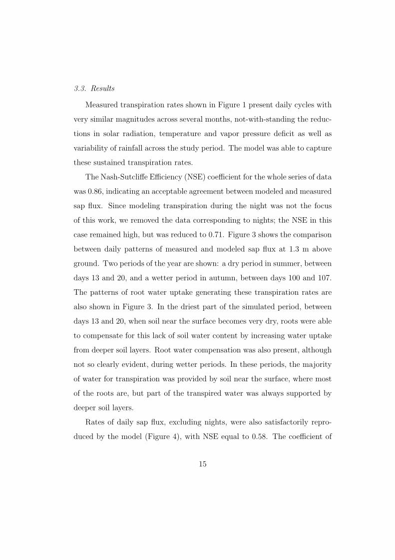
3.3. Results

Measured transpiration rates shown in Figure 1 present daily cycles with

very similar magnitudes across several months, not-with-standing the reduc-

tions in solar radiation, temperature and vapor pressure deficit as well as

variability of rainfall across the study period. The model was able to capture

these sustained transpiration rates.

The Nash-Sutcliffe Efficiency (NSE) coefficient for the whole series of data

was 0.86, indicating an acceptable agreement between modeled and measured

sap flux. Since modeling transpiration during the night was not the focus

of this work, we removed the data corresponding to nights; the NSE in this

case remained high, but was reduced to 0.71. Figure 3 shows the comparison

between daily patterns of measured and modeled sap flux at 1.3 m above

ground. Two periods of the year are shown: a dry period in summer, between

days 13 and 20, and a wetter period in autumn, between days 100 and 107.

The patterns of root water uptake generating these transpiration rates are

also shown in Figure 3. In the driest part of the simulated period, between

days 13 and 20, when soil near the surface becomes very dry, roots were able

to compensate for this lack of soil water content by increasing water uptake

from deeper soil layers. Root water compensation was also present, although

not so clearly evident, during wetter periods. In these periods, the majority

of water for transpiration was provided by soil near the surface, where most

of the roots are, but part of the transpired water was always supported by

deeper soil layers.

Rates of daily sap flux, excluding nights, were also satisfactorily repro-

duced by the model (Figure 4), with NSE equal to 0.58. The coefficient of

15

14 16 18 20

−2

−1

0

DOY

hx

(MP

a)

101 103 105 107

−2

−1

0

DOY

hx

(MP

a)

−2 −1 0

4

8

12

hx

(MPa)

Ele

vation (

m)

DOY 14

DOY 18

DOY 101

DOY 105

Figure 5: Modeled leaf water potential (continuous line) and root water potential at thesurface (dashed line) in two different periods. The panel at the bottom shows the xylempotential as a function of height above ground at 12 pm in four different days.

16

determination between modeled and observed data was 0.70, with the slope

of the least-squares regression line being 0.90 (with 95% confidence interval

ranging from 0.80 to 1.00) with an intercept of 0.17 (with 95% confidence in-

terval between 0.06 and 0.29). Figure 4 also shows the cumulative amount of

water transpired by the vegetation and that obtained from the model during

the simulated period.

Examples of modeled water potentials in the xylem are shown in Figure

5. The modeled leaf water potential oscillated around −0.2 MPa at pre-dawn

and reached values of about −3 MPa in the middle of the day. These values

are consistent with the leaf water potentials measured by Zeppel et al. [12] on

four days during the period September-December; measured pre-dawn values

for E. parramattensis and A. bakeri were between −0.18 and −1.77 MPa,

while minimum leaf water potentials were between −1.81 and −3.60 MPa. In

the same study, Zeppel et al. [12] used in their soil-plant-atmosphere model

a value of −2.8 MPa as a minimum sustainable leaf water potential, which

is consistent with the values obtained in our model. The modelled difference

between root and leaf water potentials during the night were due to both

differences in elevations (14 m = 0.14 MPa between soil surface and leaves)

and transpiration during the night. The gradient in water potentials between

roots and leaves were sufficient to generate a flux of water from the soil to

the atmosphere, such that the model did not show fluxes of water from roots

to the soil possibly associated with hydraulic redistribution. Figure 5 also

shows variation of above-ground xylem water potential for different days at

12 pm. The decrease of the xylem water potential with height is non-linear

because of the reduction in xylem conductivity (Eq. 7) caused by low leaf

17

water potentials.

4. Root water uptake with different root depths

Previous studies and the sap flux data in Figure 1 show that trees at

the site are able to maintain sustained daily sap-flux rates across several

months; the reason for this has been attributed to the continuous presence

of water near the interface between the sand and clay layers, which acts as

a buffer during dry periods [12]. Thus, when the sand becomes dry near

the surface, the trees are able to increase their water uptake from deeper

soil layers, even though a lower percentage of roots are present at these

depths. Since data on root density were available only to a depth of 1.5 m,

we modeled the root water uptake when root depths lower than 3.2 m are

assumed. We recall that in the model used by Zeppel et al. [12], which did

not account for root water compensation, a minimum root depth of 3 m was

required to satisfactorily describe the observed sap flow rates. Eucalyptus

species are generally evergreen and require deep root systems; other species

(e.g., drought deciduous species) might require shallower root depths. We

now consider root depths decreasing from a maximum of d = 3.2 m to a

minimum of d = 0.9 m, to establish whether different root depths in our

model are able to maintain the observed sap fluxes. We thus assumed that

the root distribution had the shape as in Eq. (3), modifying only the value

of d; since we used Eq. (2), this assumption implies that the root mass

remained the same in all simulations, but it was distributed differently along

the root depth.

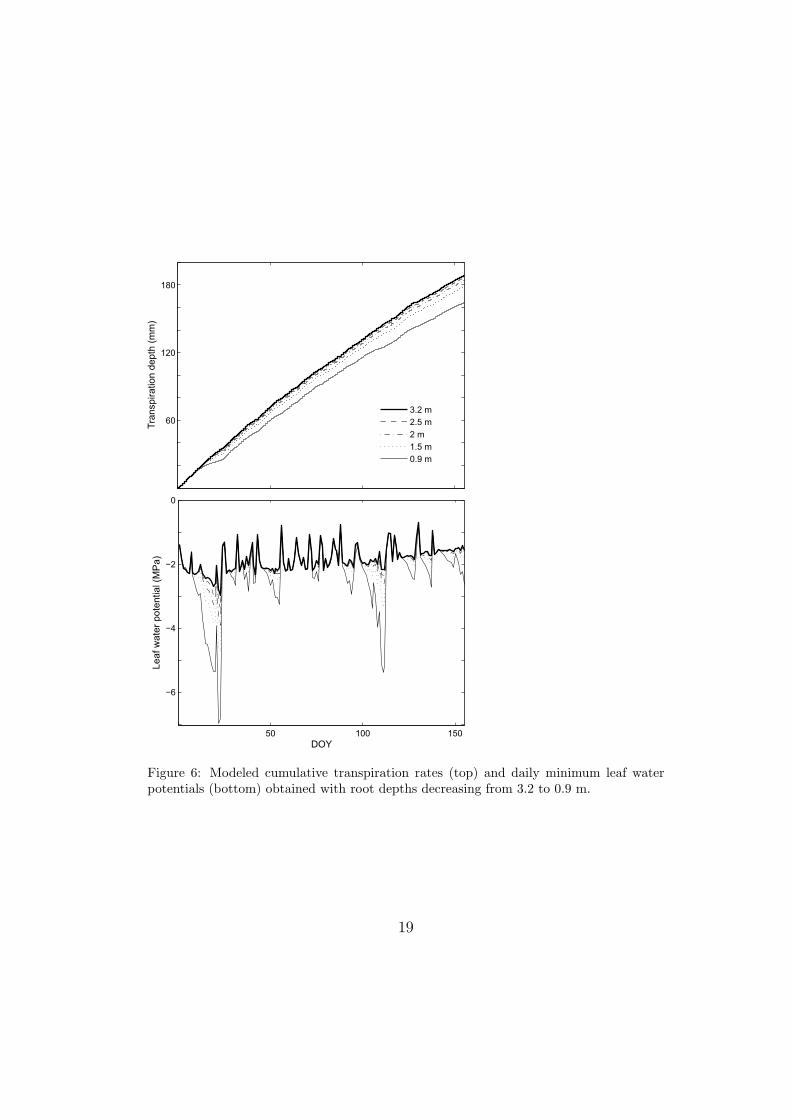
According to the model results, the water transpired over the period under

analysis decreased with shallower root depths (Figure 6). Similar transpira-

18

50 100 150

−6

−4

−2

0

DOY

Leaf w

ate

r pote

ntial (M

Pa)

3.2 m

2.5 m

2 m

1.5 m

0.9 m

60

120

180

Tra

nspiration d

epth

(m

m)

Figure 6: Modeled cumulative transpiration rates (top) and daily minimum leaf waterpotentials (bottom) obtained with root depths decreasing from 3.2 to 0.9 m.

19

tion rates were obtained with root depths from 3.2 to 2 m, while transpiration

declined more noticeably with depths lower than about 2 m. Specifically,

when assuming that the roots were almost entirely in the sandy layer (i.e.,

d = 0.9 m), the total transpiration after 155 days was about 24 mm lower

than in the case with d = 3.2 m. In order to maintain such high transpi-

ration rates even with shallower root depths, the vegetation needs to lower

the xylem water potential. As shown in Figure 6, the minimum leaf water

potential that the trees needed to sustain became much lower as root depth

decreased. The values of leaf water potential obtained with root depths lower

than about 2 m were very low and unrealistic when compared to measure-

ments at the site [12]. For all root depths, the daily minimum leaf water

potential was below hx50 for 91% of the days. With d = 3.2 m, the daily

averaged leaf water potential stayed above hx50 during the entire period sim-

ulated; as d decreased, the percentage of days in which the daily averaged

leaf water potential went below hx50 increased from 1.3%, for d = 2.5 m, to

11%, when d was 0.9 m.

The reduction in transpiration with shallower root depths is evident by

comparing the results in Figure (7) with those in Figure (3). With shallower

root depths, the vegetation was more reliant on soil moisture near the surface.

Larger water uptake rates near the surface after rainfall events caused a quick

drying of the sandy layer. With water uptake occurring mostly from the sand

layer and the high hydraulic conductivity of the sand, soil moisture content

declined near the surface inducing water stress in the vegetation. Root water

compensation was still evident during dry periods, but the lower moisture

available reduced the water uptake in comparison to the case with deeper

20

101 103 105 107

0.04

0.08

0.12

0.16

14 16 18 20

0.04

0.08

0.12

0.16

E(m

m h

−1)

Figure 7: Top: Modeled sap flux rates at 1.3 m from the ground for two different timeperiods using a total root depth of 0.9 m. Bottom: corresponding root water uptake rates,S [103d−1], profiles in the top 0.8 m from the surface.

21

root depths. Even in wetter periods, the shallow rooted vegetation is more

dependent on rainfall. This is for example shown by the rapid water uptake

near the surface occurring towards the end of the day 104, when 1 mm of

water fell in 30 minutes (Figure 7). This small event did not cause any

significant change in the root water uptake when the root depth was set to

3.2 m (Figure 3).

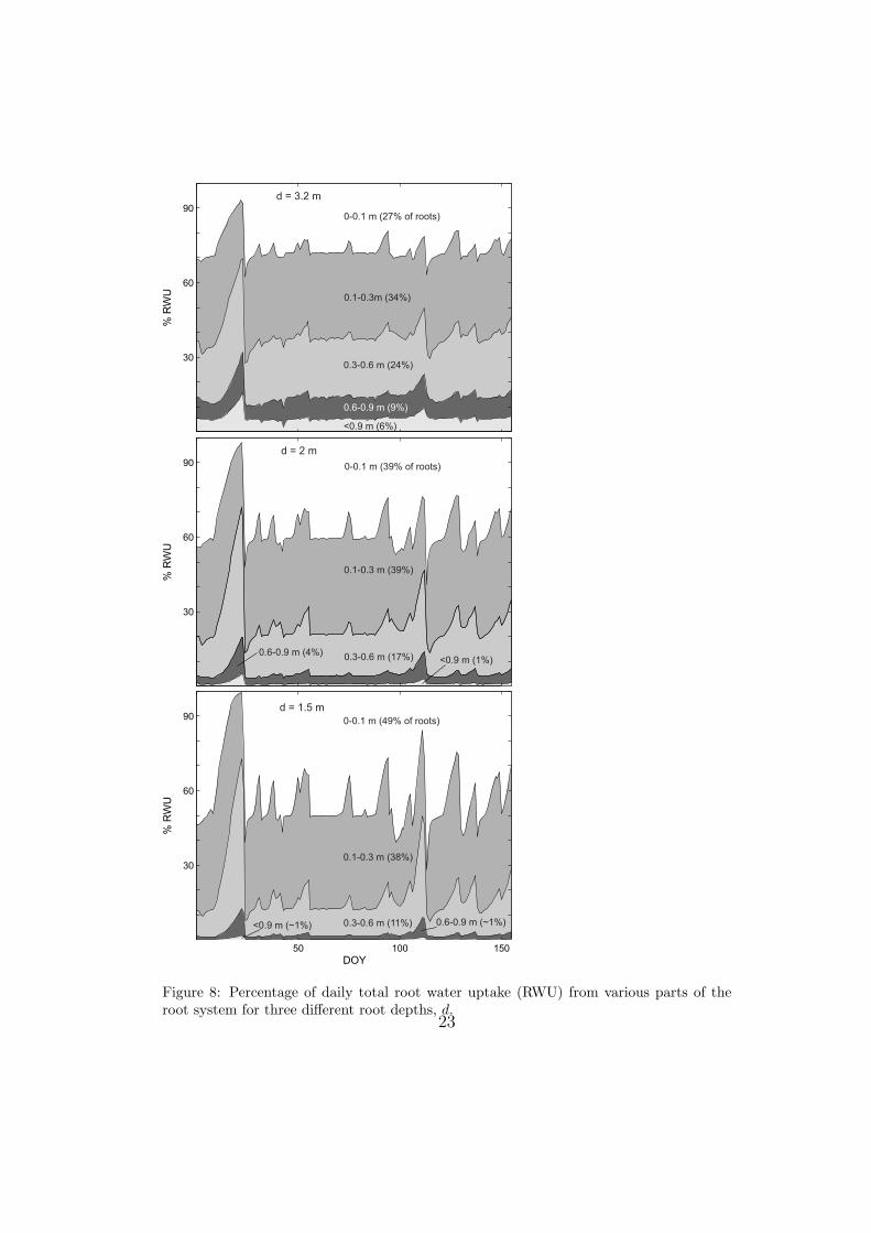
Most of the root water uptake occurred within the first 0.8 m of soil.

Figure (8) shows how daily root water uptake is partitioned among various

parts of the root system comparing different root depths. With d = 3.2 m,

about 15% of the daily root water uptake consistently came from soil layers

deeper than 0.6 m, where about 15% of the roots are; during dry periods, the

percentage of water from these depths increased, reaching about 30% in the

driest part of the period analyzed. When reducing the root depth, the roots

between 0.3 and 0.6 m became more important during dry periods. They

contributed at times more than 50% of the total daily rott water uptake,

even though less than 20% of the roots were at these depths.

To see the effect of lower rainfall rates on the partitioning of root water

uptake, we ran the same simulations using as input 70% of the rainfall rates

measured at the site (i.e., a total rainfall of 350 mm). The total transpiration

rates in this case were slightly lower than those obtained before, and these

transpiration rates were achieved thanks to lower leaf water potentials (not

shown). The partition of root water uptake from different depths did not

differ considerable from what shown in Figure (8).

22

50 100 150

30

60

90

DOY

% R

WU

30

60

90

% R

WU

30

60

90

% R

WU

d = 3.2 m

d = 2 m

d = 1.5 m

0-0.1 m (27% of roots)

0.1-0.3m (34%)

0.3-0.6 m (24%)

0.6-0.9 m (9%)

<0.9 m (6%)

0-0.1 m (39% of roots)

0.1-0.3 m (39%)

0.3-0.6 m (17%)0.6-0.9 m (4%)

<0.9 m (1%)

0.1-0.3 m (38%)

0.3-0.6 m (11%) 0.6-0.9 m (~1%)<0.9 m (~1%)

0-0.1 m (49% of roots)

Figure 8: Percentage of daily total root water uptake (RWU) from various parts of theroot system for three different root depths, d.

23

5. Conclusions

Root water compensation is the mechanism through which vegetation ad-

justs the depth of root water uptake based on soil water availability, thereby

favoring uptake from areas of the soil that have higher water potentials even

when the root density is relatively low in these areas. We present here a

modeling study that helps show the key role of root water compensation in

maintaining sustained transpiration rates in an Australian woodland growing

on a duplex soil.

Using a one dimensional model that couples water flow in the soil to that

in the xylem, we were able to reproduce field observations of transpiration

rates over a period of several months. The root depth in this simulation

was initially assumed to be 3.2 m; this value was adopted in a previous

study at the same site [12]. Root water uptake from the model suggested

that root water compensation was a key mechanism that allowed trees to

maintain stable transpiration rates during dry periods of the year; root water

compensation was also present during relatively wet periods. The roots below

a depth of 0.6 m, totaling to about 15% of the whole root biomass, provided

consistently nearly 15% of the daily transpiration, reaching 30% in the driest

part of the analyzed period.

The roots below a depth of 0.6 m, totaling to about 15% of the whole

root biomass, provided between 15% and 30% of the daily transpiration.

Scenarios with different root depths, from 3.2 to 0.9 m, showed that in all

cases root water compensation was actively involved in sustaining transpira-

tion rates, which anyway reduced considerably for root depths shallower than

about 2 m. For such depths, transpiration rates were sustained by decreasing

24

leaf water potentials, which were much lower than what was experimentally

observed. The model suggested that the vegetation with shallower root sys-

tem is more responsive to rainfall events; in this case the soil surface becomes

drier and vegetation is more prone to experience water stress, thereby reduc-

ing transpiration rates. Root depths shallower than 2 m, with a percentage

of root biomass below 0.6 m of less than about 5%, reduced transpiration

rates because of water stress and led to leaf water potentials much lower than

field observations. In those scenarios, roots deeper than 0.3 m provided up

to 70% of the daily transpiration even though root biomass at these depths

was less than 15%.

Our results can likely be extended to other areas with duplex soils and

shallow water table conditions, where large amounts of water can be reached

by the roots. In such conditions, roots can switch their preferential water

uptake from near the surface immediately after rainfall events to deeper soil

layers, where the wet soil allows for larger differences between soil and root

water potentials. Our study thus shows that duplex soils might provide ener-

getically favorable conditions for root water uptake near the interface between

the layers, thereby allowing vegetation to maintain sustained transpiration

rates not-with-standing intermittent wet and dry periods.

Appendix A. Water retention curves

In unsaturated conditions, the soil moisture (θ) and unsaturated hydraulic

conductivity (k) vary with soil pressure head (hs). The relationship between

these variables are modeled as [36]:

25

θ =

θr +

θs − θr[1 + |αhs|n]m

if hs < 0,

θs if hs ≥ 0,

(A.1)

k =

ks

(θ − θrθs − θr

)l[1−

(1−

(θ − θrθs − θr

)1/m)m]2

if hs < 0,

ks if hs ≥ 0,

(A.2)

where θr [L3L−3] is the residual water content, θs [L

3L−3] is the water content

at saturation, ks[LT−1] is the soil hydraulic conductivity at saturation and

α[L−1], l[−], n[−] are parameters dependent on soil type; the parameterm[−]

is equal to 1− 1/n.

Appendix B. Penman-Monteith equation

The Penman-Monteith equation reads:

Ep =

[Qn∆+ CpDga

λ[∆gc + γ(gc + ga)]

]gc, (B.1)

where Ep [LT−1] is the transpiration rate, Qn [MT−3] is the net radiation,

∆ [ML−1T−2K−1] is the slope of the saturation vapor pressure curve at a

given air temperature, Cp [ML−1T−2K−1] is the heat capacity of air at con-

stant pressure, D [ML−1T−2] is the vapour pressure deficit, λ [ML−1T−2] is

26

the latent heat of vaporization, ga [LT−1] is the aerodynamic conductance,

γ [ML−1T−2K−1] is the psychrometric constant and gc [LT−1] is the canopy

conductance. The net radiation is calculated as the 70% of the total radia-

tion, S [49]. The slope of the saturation vapor pressure curve, ∆, is obtained

as [50]:

∆ =

[4098

(Ta − 35.85)2

]esat, (B.2)

where esat [ML−1T−2] is the saturation vapor pressure at a given air temper-

ature Ta [K], and given by the equation [50]:

esat = 611 exp

[17.27(Ta − 273.15)

(Ta − 35.85)

], (B.3)

with esat in Pascal.

The canopy conductance, gc, was modeled as:

gc =

[gsgb

gs + gb

]LAI, (B.4)

where LAI [−] is the leaf area index, gb [LT−1] is the leaf boundary layer

conductance per unit leaf area and gs [LT−1] is the stomatal conductance.

Assuming that CO2 concentrations remain constant and do not affect the

stomatal conductance, gs can be modeled as [51]:

gs = gsmaxf(S)f(Ta)f(D)f(hxleaf ), (B.5)

27

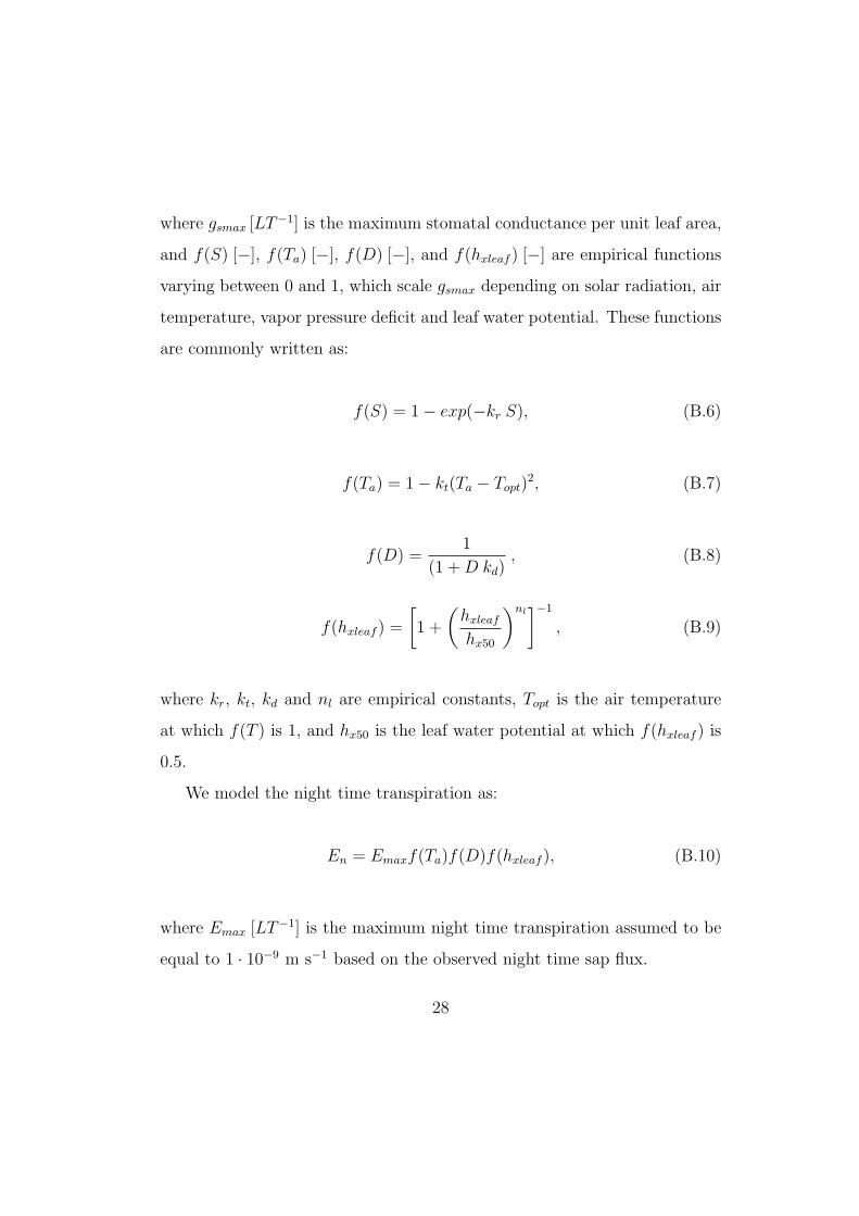
where gsmax [LT−1] is the maximum stomatal conductance per unit leaf area,

and f(S) [−], f(Ta) [−], f(D) [−], and f(hxleaf ) [−] are empirical functions

varying between 0 and 1, which scale gsmax depending on solar radiation, air

temperature, vapor pressure deficit and leaf water potential. These functions

are commonly written as:

f(S) = 1− exp(−kr S), (B.6)

f(Ta) = 1− kt(Ta − Topt)2, (B.7)

f(D) =1

(1 +D kd), (B.8)

f(hxleaf ) =

[1 +

(hxleaf

hx50

)nl]−1

, (B.9)

where kr, kt, kd and nl are empirical constants, Topt is the air temperature

at which f(T ) is 1, and hx50 is the leaf water potential at which f(hxleaf ) is

0.5.

We model the night time transpiration as:

En = Emaxf(Ta)f(D)f(hxleaf ), (B.10)

where Emax [LT−1] is the maximum night time transpiration assumed to be

equal to 1 · 10−9 m s−1 based on the observed night time sap flux.

28

Appendix C. Water flow in above ground xylem

Above ground, for a single plant, the water flow through the xylem can

be written as [52, 53]:

ρg Ss

(∂hx

∂t

)− 1

A(z)

∂

∂z

[kp(hx, z)A(z)

(∂hx

∂z+ 1

)]=

− 1

A(z)τ(z) Ed(z, t, hx), (C.1)

whereA(z)[L2] is the cross-sectional area of the above ground xylem, kp[LT−1]

is the xylem conductivity per unit of xylem cross-sectional area, τ(z) [L] is

the leaf area per unit of stem length, and Ed(z, t, hx) [LT−1] is the transpira-

tion flux density. For simplicity, we assume a uniform xylem cross sectional

area above ground, and thus A(z) becomes a constant. Therefore, A(z) on

the l.h.s. of Eq. (C.1) at the numerator and denominator cancel each other.

Since we do not consider a canopy structure, the term on the r.h.s of Eq.

(C.1) becomes zero.

Because Eqs. (1) and (5) define transpiration per unit of ground area,

we need to re-scale Eq. (C.1) from the xylem cross-sectional area of a single

plant to the unit of ground area. This is obtained by re-scaling the axial

hydraulic conductivity, kp, which is multiplied by the ratio Ax/As, where Ax

is the average xylem cross-sectional area of all the plants in the ground area

As. Accordingly, Eq. (C.1) becomes Eq. (6).

29

1 2 3

−3

−2

−1

0

root density (m−1

)

Depth

(m)

Figure D.9: Modeled root distribution with d = 3.2 m (continuous line) and measureddistribution (circles) [40].

Appendix D. Estimated root distribution

The root distribution when the root depth equals 3.2 m was estimated

from the data presented in Figure 4 of Macinnis-Ng et al. [40]. The percentage

of roots at 0.1, 0.3, 0.5, 1.0, and 1.5 m was measured in four trenches. We

averaged the results from the four trenches and assumed that the percentage

of roots at 0.1 m was distributed over the first 0.15 m of soil; the value at 0.3

m referred to the soil between 0.15 and 0.40 m, the value at 0.5 m referred

to the soil between 0.40 and 0.75 m, the value at 1.0 m referred to the soil

between 0.75 and 1.25 m, and the value at 1.5 m referred to the depths

between 1.25 and 1.75 m. Dividing the values of the averaged percentage

of roots by the respective depth interval gives and estimation of the root

density.

The parameter qz of the root distribution (Eq. 2) with d = 3.2 m was

chosen to fit the root estimated from these calculation, as shown in Figure

30

D.9.

Acknowledgements

The authors thank Melanie J. B. Zeppel for providing the data used in

the study. P.V., D.E. and E.D. acknowledge the support of the Australian

Research Council (ARC) and the Australian National Water Commission

(NWC) through Program 4 (Groundwater Vegetation Atmosphere Interac-

tions) of the National Centre for Groundwater Research and Training. P.V.

thanks the Director of the National Environmental Engineering Research

Institute, Nagpur, India, for granting leave to pursue his PhD studies at

Monash University.

References

[1] G. Bonan, Ecological Climatology: Concepts and Applications, Cam-

bridge University Press, Cambridge, UK, 2002.

[2] L. M. Arya, G. R. Blake, D. A. Farrell, Field study of soil-water depletion

patterns in presence of growing soybean roots. 3. Rooting characteristics

and root extraction of soil-water, Soil Science Society of America Journal

39 (3) (1975) 437–444.

[3] J. U. Nnyamah, T. A. Black, Rates and patterns of water-uptake in a

Douglas-fir forest, Soil Science Society of America Journal 41 (5) (1977)

972–979.

[4] S. R. Green, B. E. Clothier, Root water uptake by kiwifruit vines fol-

lowing partial wetting of the root zone, Plant and Soil 173 (2) (1995)

317–328.

31

[5] E. H. McLean, M. Ludwig, P. F. Grierson, Root hydraulic conductance

and aquaporin abundance respond rapidly to partial root-zone drying

events in a riparian Melaleuca species, New Phytologist 192 (3) (2011)

664–675, doi:10.1111/j.1469-8137.2011.03834.x.

[6] M. M. Caldwell, T. E. Dawson, J. H. Richards, Hydraulic lift: Conse-

quences of water efflux from the roots of plants, Oecologia 113 (2) (1998)

151–161.

[7] R. J. Ryel, M. M. Caldwell, C. K. Yoder, D. Or, A. J. Leffler, Hydraulic

redistribution in a stand of Artemisia tridentata: evaluation of benefits

to transpiration assessed with a simulation model, Oecologia 130 (2)

(2002) 173–184, doi:10.1007/s004420100794.

[8] I. Prieto, Z. Kikvidze, F. I. Pugnaire, Hydraulic lift: Soil processes and

transpiration in the Mediterranean leguminous shrub Retama sphaero-

carpa (L.) Boiss, Plant and Soil 329 (1) (2010) 447–456.

[9] L. H. Li, Y. P. Wang, Q. Yu, B. Pak, D. Eamus, J. H. Yan, E. van Gorsel,

I. T. Baker, Improving the responses of the Australian community land

surface model (CABLE) to seasonal drought, Journal of Geophysical

Research-Biogeosciences 117, doi:10.1029/2012jg002038.

[10] A. J. Guswa, Canopy vs. roots: Production and destruction of variability

in soil moisture and hydrologic fluxes, Vadose Zone Journal 11 (3).

[11] F. Orellana, P. Verma, S. P. I. Loheide, E. Daly, Monitoring and Mod-

eling Water-Vegetation Interaction in Groundwater-Dependent Ecosys-

tems, Reviews of Geophysics 50 (RG3003) (2012) 1–24.

32

[12] M. Zeppel, C. MacInnis-Ng, A. Palmer, D. Taylor, R. Whitley,

S. Fuentes, I. Yunusa, M. Williams, D. Eamus, An analysis of the sen-

sitivity of sap flux to soil and plant variables assessed for an Australian

woodland using a soil-plant-atmosphere model, Functional Plant Biol-

ogy 35 (6) (2008) 509–520.

[13] N. J. Jarvis, A simple empirical model of root water-uptake, Journal of

Hydrology 107 (1-4) (1989) 57–72, doi:10.1016/0022-1694(89)90050-4.

[14] M. Javaux, V. Couvreur, J. Vander Borght, H. Vereecken, Root

Water Uptake: From Three-Dimensional Biophysical Processes to

Macroscopic Modeling Approaches, Vadose Zone Journal 12 (4), doi:

10.2136/vzj2013.02.0042.

[15] N. J. Jarvis, Simple physics-based models of compensatory plant wa-

ter uptake: concepts and eco-hydrological consequences, Hydrology and

Earth System Sciences 15 (11) (2011) 3431–3446, doi:10.5194/hess-15-

3431-2011.

[16] J. A. Vrugt, M. T. VanWijk, J. W. Hopmans, J. imunek, One-, two-, and

three-dimensional root water uptake functions for transient modeling,

Water Resources Research 37 (10) (2001) 2457–2470.

[17] J. A. Vrugt, J. W. Hopmans, J. Simunek, Calibration of a Two-

Dimensional Root Water Uptake Model, Soil Sci. Soc. Am. J. 65 (4)

(2001) 1027–1037, doi:10.2136/sssaj2001.6541027x.

[18] T. Skaggs, M. van Genuchten, P. Shouse, J. Poss, Macroscopic ap-

33

proaches to root water uptake as a function of water and salinity stress,

Agricultural Water Management 86 (1-2) (2006) 140–149.

[19] K. Y. Li, R. De Jong, J. B. Boisvert, An exponential root-water-uptake

model with water stress compensation, Journal of Hydrology 252 (1-4)

(2001) 189–204.

[20] B. K. Yadav, S. Mathur, M. A. Siebel, Soil moisture dynamics model-

ing considering the root compensation mechanism for water uptake by

plants, Journal of Hydrologic Engineering 14 (9) (2009) 913–922.

[21] J. Simunek, J. W. Hopmans, Modeling compensated root water and

nutrient uptake, Ecological Modelling 220 (4) (2009) 505–521, doi:

10.1016/j.ecolmodel.2008.11.004.

[22] M. Siqueira, G. Katul, A. Porporato, Onset of water stress, hysteresis in

plant conductance, and hydraulic lift: Scaling soil water dynamics from

millimeters to meters, Water Resources Research 44 (W01432) (2008)

1–14, doi:W01432 10.1029/2007wr006094.

[23] M. Siqueira, G. Katul, A. Porporato, Soil Moisture Feedbacks on Con-

vection Triggers: The Role of Soil-Plant Hydrodynamics, Journal of

Hydrometeorology 10 (1) (2009) 96–112, doi:10.1175/2008jhm1027.1.

[24] S. Tron, F. Laio, L. Ridolfi, Plant water uptake strategies to cope with

stochastic rainfall, Advances in Water Resources 53 (2013) 118–130, doi:

10.1016/j.advwatres.2012.10.007.

[25] T. Vogel, M. Dohnal, J. Dusek, J. Votrubova, M. Tesar, Macroscopic

34

Modeling of Plant Water Uptake in a Forest Stand Involving Root-

Mediated Soil Water Redistribution, Vadose Zone Journal 12 (1), doi:

10.2136/vzj2012.0154.

[26] M. Mendel, S. Hergarten, H. J. Neugebauer, On a better understanding

of hydraulic lift: A numerical study, Water Resources Research 38 (10)

(2002) 11–110.

[27] G. G. Amenu, P. Kumar, A model for hydraulic redistribution incorpo-

rating coupled soil-root moisture transport, Hydrology and Earth Sys-

tem Sciences 12 (1) (2008) 55–74.

[28] J. C. Quijano, P. Kumar, D. T. Drewry, A. Goldstein, L. Misson, Com-

petitive and mutualistic dependencies in multispecies vegetation dy-

namics enabled by hydraulic redistribution, Water Resources Research

48 (W05518) (2012) 1–22, doi:W05518 10.1029/2011wr011416.

[29] S. Gou, G. Miller, A groundwatersoilplantatmosphere continuum ap-

proach for modelling water stress, uptake, and hydraulic redistribution

in phreatophytic vegetation, Ecohydrology 7 (3) (2013) 1029–1041, doi:

10.1002/eco.1427.

[30] Q. D. van Lier, J. C. van Dam, K. Metselaar, R. de Jong, W. H. M.

Duijnisveld, Macroscopic root water uptake distribution using a matric

flux potential approach, Vadose Zone Journal 7 (3) (2008) 1065–1078,

doi:10.2136/vzj2007.0083.

[31] N. J. Jarvis, Comment on ”Macroscopic Root Water Uptake Distribu-

35

tion Using a Matric Flux Potential Approach”, Vadose Zone Journal

9 (2) (2010) 499–502, doi:10.2136/vzj2009.0148.

[32] C. Doussan, A. Pierret, E. Garrigues, L. Pages, Water uptake by plant

roots: II - Modelling of water transfer in the soil root-system with ex-

plicit account of flow within the root system - Comparison with experi-

ments, Plant and Soil 283 (1-2) (2006) 99–117, doi:10.1007/s11104-004-

7904-z.

[33] G. Bohrer, H. Mourad, T. A. Laursen, D. Drewry, R. Avissar, D. Poggi,

R. Oren, G. G. Katul, Finite element tree crown hydrodynamics model

(FETCH) using porous media flow within branching elements: A

new representation of tree hydrodynamics, Water Resources Research

41 (W11404) (2005) 1–17, doi:10.1029/2005wr004181.

[34] M. Janott, S. Gayler, A. Gessler, M. Javaux, C. Klier, E. Priesack,

A one-dimensional model of water flow in soil-plant systems based

on plant architecture, Plant and Soil 341 (1-2) (2011) 233–256, doi:

10.1007/s11104-010-0639-0.

[35] S. Bittner, N. Legner, F. Beese, E. Priesack, Individual tree branch-

level simulation of light attenuation and water flow of three F. sylvatica

L. trees, Journal of Geophysical Research-Biogeosciences 117 (G01037)

(2012) 1–17.

[36] M. T. van Genuchten, Closed-form equation for predicting the hydraulic

conductivity of unsaturated soils, Soil Science Society of America Jour-

nal 44 (5) (1980) 892–898.

36

[37] R. A. Feddes, P. Kowalik, K. Kolinska-Malinka, H. Zaradny, Simula-

tion of field water uptake by plants using a soil water dependent root

extraction function, Journal of Hydrology 31 (1-2) (1976) 13–26.

[38] N. W. Pammenter, C. Vander Willigen, A mathematical and statistical

analysis of the curves illustrating vulnerability of xylem to cavitation,

Tree Physiology 18 (8-9) (1998) 589–593.

[39] M. Zeppel, D. Tissue, D. Taylor, C. Macinnis-Ng, D. Eamus, Rates of

nocturnal transpiration in two evergreen temperate woodland species

with differing water-use strategies, Tree Physiology 30 (8) (2010) 988–

1000, doi:10.1093/treephys/tpq053.

[40] C. M. O. Macinnis-Ng, S. Fuentes, A. P. O’Grady, A. R. Palmer, D. Tay-

lor, R. J. Whitley, I. Yunusa, M. J. B. Zeppel, D. Eamus, Root biomass

distribution and soil properties of an open woodland on a duplex soil,

Plant and Soil 327 (1-2) (2010) 377–388, doi:10.1007/s11104-009-0061-7.

[41] C. Macinnis-Ng, M. Zeppel, M. Williams, D. Eamus, Applying a SPA

model to examine the impact of climate change on GPP of open wood-

lands and the potential for woody thickening, Ecohydrology 4 (3) (2011)

379–393, doi:10.1002/eco.138.

[42] I. A. Yunusa, M. J. Zeppel, S. Fuentes, C. M. Macinnis-Ng, A. R. Palmer,

D. Eamus, An assessment of the water budget for contrasting vegetation

covers associated with waste management, Hydrological Processes 24 (9)

(2010) 1149–1158.

37

[43] I. A. M. Yunusa, S. Zolfaghar, M. J. B. Zeppel, Z. Li, A. R. Palmer,

D. Eamus, Fine Root Biomass and Its Relationship to Evapotranspira-

tion in Woody and Grassy Vegetation Covers for Ecological Restoration

of Waste Storage and Mining Landscapes, Ecosystems 15 (1) (2012)

113–127, doi:10.1007/s10021-011-9496-9.

[44] R. F. Carsel, R. S. Parrish, Developing joint probability-distributions

of soil-water retention characteristics, Water Resources Research 24 (5)

(1988) 755–769, doi:10.1029/WR024i005p00755.

[45] R. H. Froend, P. L. Drake, Defining phreatophyte response to reduced

water availability: Preliminary investigations on the use of xylem cavi-

tation vulnerability in Banksia woodland species, Australian Journal of

Botany 54 (2) (2006) 173–179.

[46] E. Daly, A. Porporato, I. Rodriguez-Iturbe, Coupled dynamics of photo-

synthesis, transpiration, and soil water balance. Part I: Upscaling from

hourly to daily level, Journal of Hydrometeorology 5 (3) (2004) 546–558.

[47] L. D. Prior, D. Eamus, Seasonal changes in hydraulic conductance,

xylem embolism and leaf area in Eucalyptus tetrodonta and Eucalyptus

miniata saplings in a north Australian savanna, Plant, Cell and Envi-

ronment 23 (9) (2000) 955–965, doi:10.1046/j.1365-3040.2000.00612.x.

[48] B. E. Medlyn, R. A. Duursma, D. Eamus, D. S. Ellsworth, I. C. Prentice,

C. V. M. Barton, K. Y. Crous, P. De Angelis, M. Freeman, L. Wingate,

Reconciling the optimal and empirical approaches to modelling stom-

38

atal conductance, Global Change Biology 17 (6) (2011) 2134–2144, doi:

10.1111/j.1365-2486.2010.02375.x.

[49] J. P. Lhomme, E. Elguero, A. Chehbouni, G. Boulet, Stomatal con-

trol of transpiration: Examination of Monteith’s Formulation of canopy

resistance, Water Resources Research 34 (9) (1998) 2301–2308, doi:

10.1029/98WR01339.

[50] R. Allen, M. Smith, L. Pereira, A. Perrier, An update for the calculation

of reference evapotranspiration, ICID bulletin 43 (2) (1994) 35–92.

[51] P. G. Jarvis, The Interpretation of the Variations in Leaf Water Potential

and Stomatal Conductance Found in Canopies in the Field, Philosoph-

ical Transactions of the Royal Society of London. Series B, Biological

Sciences 273 (927) (1976) 593–610.

[52] T. Kumagai, Modeling water transportation and storage in sapwood -

model development and validation, Agricultural and Forest Meteorology

109 (2) (2001) 105–115, doi:10.1016/s0168-1923(01)00261-1.

[53] Y. L. Chuang, R. Oren, A. L. Bertozzi, N. Phillips, G. G. Katul, The

porous media model for the hydraulic system of a conifer tree: Linking

sap flux data to transpiration rate, Ecological Modelling 191 (3-4) (2006)

447–468, doi:10.1016/j.ecolmodel.2005.03.027.

39