Embed Size (px)
Citation preview

Cosmology from optical interferometry of AGNs ... in the visible
Optical Interferometry in the VisibleOCA, Nice, January 15-16, 2015
Romain G. Petrov, Lagrange Laboratory (OCA, UNS, CNRS), Nice, France
withSuvendu Rakshit, Florentin Millour, Sebastian Hoënig, Anthony Meilland, Stephane Lagarde, Makoto Kishimoto,
Alessandro Marconi, Walter Jaffe, Gerd Weigelt...

Introduction:
• Structure and physics of AGNs
January 16, 2015 OIV 2015 Optical interferometry of AGNs in the Visible R.G. Petrov 2

Typical scales
• Accretion disk: ld(s) mas indirect constraints from luminosity distribution
• BLR: 100 ld(s) 0.01 – 0.1 mas imaging requires 1-10 km baselines in V Reverberation mapping constraints on geometry and kinematics with cosmological potential
differential interferometry in K band better differential interferometry in V ?
• Torus (inner rim): 0.5-1pc 0.05 – 5 mas a few images with MATISSE in L band Gas “in the torus” could be
imaged in V and constrain torus kinematics Relationship with BLR ?
• NLR (inner outflow): 1-10 pc (?) 0.05-50 mas imagingBLR like scaling functions with
luminosity ?January 16, 2015 OIV 2015 Optical interferometry of AGNs in the Visible R.G. Petrov 3

Outline
• Focus on BLR observations• Reverberation Mapping
– size-luminosity law and cosmology– mass-luminosity law and SMBH and Galactic evolution
• Interferometric direct distance measurements from Dust– Complexity of geometry and need for a new unification step
• Differential interferometry of BLRs• The observed is not that was expected: the 3C273 case• The potential of the K band• The potential of the Visible, with UTs, ATs and a post VLTI interferometer• Conclusion
January 16, 2015 OIV 2015 Optical interferometry of AGNs in the Visible R.G. Petrov 4

Reverberation mapping
5January 16, 2015 OIV 2015 Optical interferometry of AGNs in the Visible R.G. Petrov

Reverberation Mapping, cosmology and galactic evolution
• Structure and physics of AGNs• Reverberation mapping yields Size-luminosity and Mass-luminosity laws• Mass-luminosity laws from variability• Use QSO as standard candles and mass tags• Geometry dependent laws
January 16, 2015 OIV 2015 Optical interferometry of AGNs in the Visible R.G. Petrov 6
Bentz, A&A, 2013
Kaspi, A&A, 2000

January 16, 2015 OIV 2015 Optical interferometry of AGNs in the Visible R.G. Petrov 7

A complex, luminosity dependent structure
January 16, 2015 OIV 2015 Optical interferometry of AGNs in the Visible R.G. Petrov 8
Kish
imo
to, O
CA
, 20
13
Can we consider a “grand unification” involving luminosity and luminosity as a function of latitude ?

Differential interferometry of BLR
January 16, 2015 OIV 2015 Optical interferometry of AGNs in the Visible R.G. Petrov 9
• Images on resolved sources• Unresolved source:
• Differential Visibility =size of the bin
• Differential phase =position of the bin
Rakshit, MNRAS, 2015

Differential interferometry and RM:RM signals
Full degeneracy between– inclination– opening angle– local velocity field (turbulence)
January 16, 2015 OIV 2015 Optical interferometry of AGNs in the Visible R.G. Petrov 10
inclination
opening
Ra
kshit, M
NR
AS
, 20
15
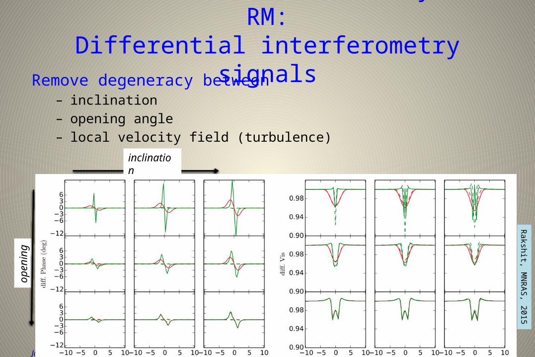
Differential interferometry and RM:Differential interferometry signals
Remove degeneracy between– inclination– opening angle– local velocity field (turbulence)
January 16, 2015 OIV 2015 Optical interferometry of AGNs in the Visible R.G. Petrov 11
inclination
opening
Ra
kshit, M
NR
AS
, 20
15

12
Differential interferometry of BLRs: 3C273• Brightest “nearby” QSO, K=9.7, L=6 1046 erg/s.
– K=9.8 in continuum; K=9.2 on top of line
• z=0.16– Paa line at 2.17 microns
• Reverberation mapping radius: 240 to 580 ld– RBLR=307-91
+69 ld = 0.10 mas in Hg
– RBLR=514-65+64 ld = 0.16 mas in Ha
• MBH~ 2 to 5 108 Msun (Kaspi, 2000)
– ~ 60 108 Msun, (Paltani, 2005)
• Radius of inner rim of torus– RT 0.81±0.34 pc=0.30±0.12 mas (Kishimoto 2011)
• VLTI resolution in K band: 3.5 mas
– Very unresolved target• Differential Interferometry
– Too faint for standard AMBER operation
• MR limiting magnitude set by fringe tracker <8.5
January 16, 2015 OIV 2015 Optical interferometry of AGNs in the Visible R.G. Petrov

3C273: what did we expect?
January 16, 2015 OIV 2015 Optical interferometry of AGNs in the Visible R.G. Petrov 13
For a flat Keplerian model and RBLR=0.15 mas
• Differential visibility up to 2%
• Differential phase up to 4°• i.e. 40 mas photocenter displacement• up to 2° if jet direction is BLR axis
jet
Pe
tro
v, H
ires
20
14

3C273 measures
• Differential visibility accuracy <0.01 per channel
• Visibility drops on all baselines (SNR=10 on largest baseline)
• Differential visibility drop extends over full line
• Differential phase = 0±0.5° per channel of 1250 km/s
January 16, 2015 OIV 2015 Optical interferometry of AGNs in the Visible R.G. Petrov 14
resolution=240
resolution=480
Pe
tro
v, H
ires
20
14
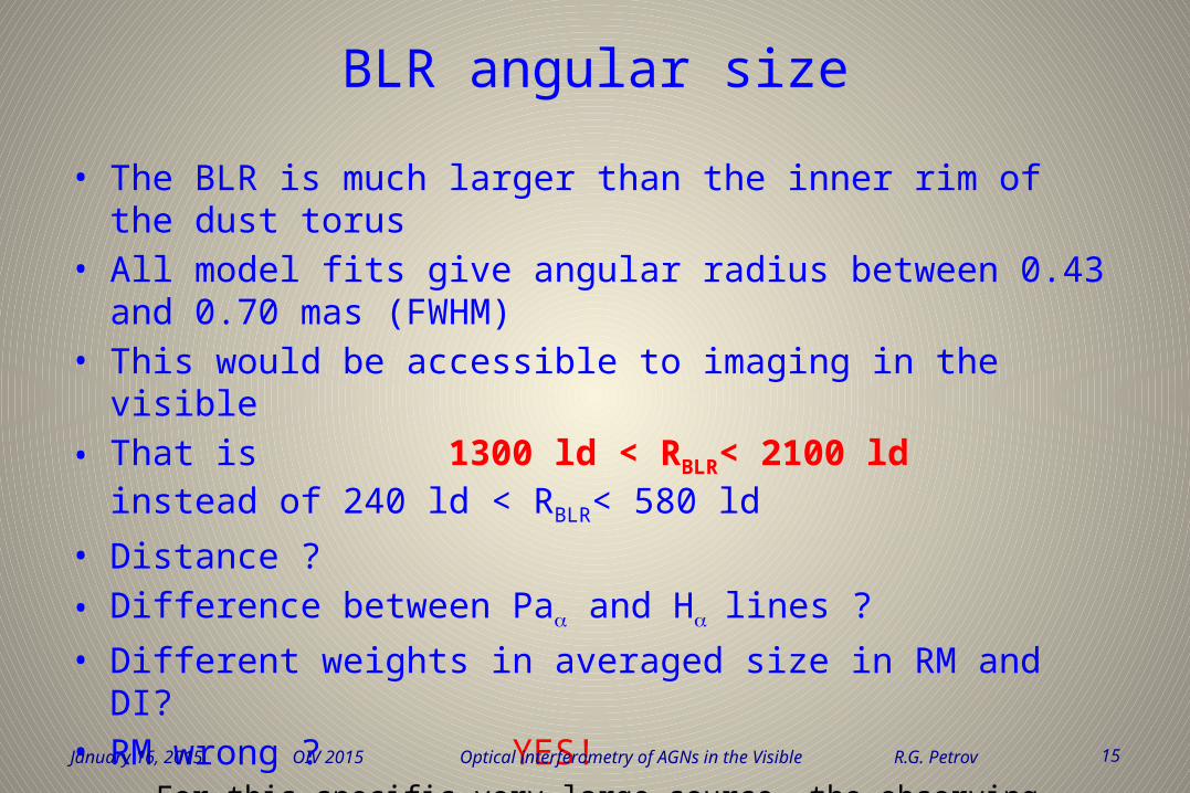
BLR angular size
• The BLR is much larger than the inner rim of the dust torus• All model fits give angular radius between 0.43 and 0.70 mas (FWHM)• This would be accessible to imaging in the visible• That is 1300 ld < RBLR< 2100 ld instead of 240 ld < RBLR< 580 ld • Distance ?• Difference between Paa and Ha lines ?• Different weights in averaged size in RM and DI?• RM wrong ? YES!
– For this specific very large source, the observing time window (2300 days is too short to properly measure any delay larger than 800 days)
January 16, 2015 OIV 2015 Optical interferometry of AGNs in the Visible R.G. Petrov 15

Biased Reverberation Mapping of 3C273
• Take 3C273 continuum light curve (S. Kaspi et al, ApJ 2000)• Produce 500 interpolations of this light curve (damped random walk model, Y. Zu et
al, ApJ 2011)• For each continuum light curve, produce a line light curve, with a time delay tin.
• Compute the RM cross-correlation function, deduce a measured time delay tout and plot tout = f(tin).
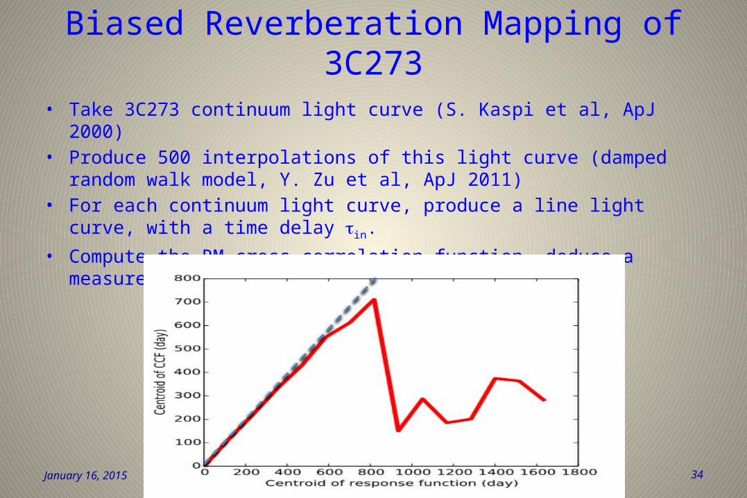
• Reverberation Mapping with the 3C273 observation window, cannot measure BLR sizes larger than 800 light days. – For larger time lags, it yields BLR size estimates in 200-500 ld range– Other interpolation methods give similar results
January 16, 2015 OIV 2015 Optical interferometry of AGNs in the Visible R.G. Petrov 16
Pe
trov, H
ires 2
01
4

BLR model
• “cloud list” model• Radial distribution and RBLR
• Inclination• Opening angle• Local line profile(s) & width• Turbulent velocity• Rotation velocity law
(Keplerian)• Radial velocity law• ...
January 16, 2015 OIV 2015 Optical interferometry of AGNs in the Visible R.G. Petrov 17
Ra
ksh
it, M
NR
AS
, 2
01
5

Global fit
January 16, 2015 OIV 2015 Optical interferometry of AGNs in the Visible R.G. Petrov 18
• RBLR=0.63±0.1 mas– RBLR=0.63±0.1 mas
– RBLR=1880±30 ld
• Inclination not really constrained below i<15°
• Opening angle larger than 85°• Turbulent velocity field 1500
km/s• Mass little sensitive to
inclination: MBH=5.4-0.4+0.2 Msun
Add 20% relative error to RBLR and to MBH because of uncertainty on (absolute visibility in continuum inner rim size)
Pe
tro
v, H
ires
20
14
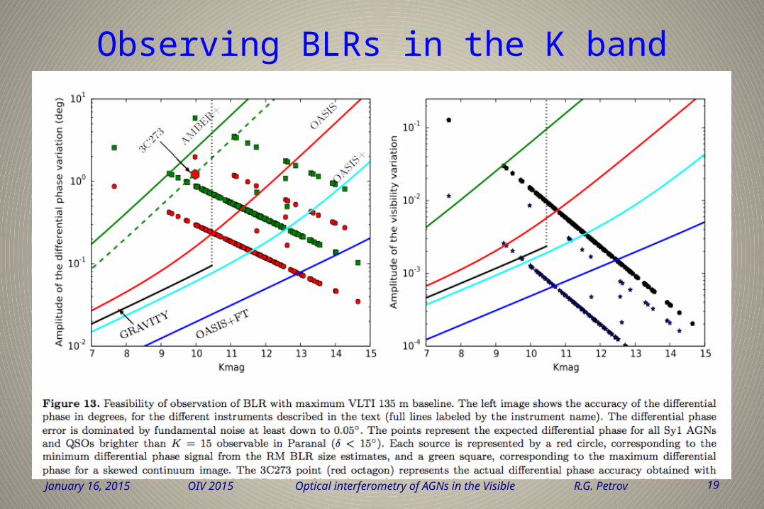
Observing BLRs in the K band
January 16, 2015 OIV 2015 Optical interferometry of AGNs in the Visible R.G. Petrov 19

Observing AGNs in the Visible
January 16, 2015 OIV 2015 Optical interferometry of AGNs in the Visible R.G. Petrov 20
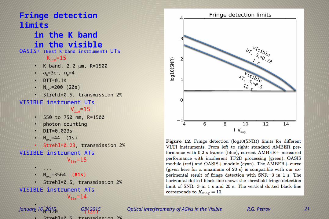
Fringe detection limitsin the K bandin the visible
OASIS+ (Best K band instrument) UTs Klim=15• K band, 2.2 mm, R=1500• sR=3e-, np=4• DIT=0.1s • Nexp=200 (20s)• Strehl=0.5, transmission 2%
VISIBLE instrument UTs Vlim=15• 550 to 750 nm, R=1500• photon counting• DIT=0.023s• Nexp=44 (1s)• Strehl=0.23, transmission 2%
VISIBLE instrument ATs Vlim=15• ...• Nexp=3564 (81s)• Strehl=0.5, transmission 2%
VISIBLE instrument ATs Vlim=14• ...• N=120 (12s)• Strehl=0.5, transmission 2%
January 16, 2015 OIV 2015 Optical interferometry of AGNs in the Visible R.G. Petrov 21
Vmag
VisibleUT, St =0.231 s
VisibleAT, St=0.512 s

Target list
• We investigate all QSOs and Sy1 AGNs observable at Paranal (d<15°)• With Kmag<15 and Vmag<15 ~ 130 targets
January 16, 2015 OIV 2015 Optical interferometry of AGNs in the Visible R.G. Petrov 22

Observing BLRs in the Visible• UTs Str~0.25 between 0.55 and 0.75 nm R=1500 2 hours
– sf(V=15) ~ sf(K=15) if StrK=0.5 and StrV=0.23
– FdiffV = FdiffK*50 (resolution gain and use of H a instead of Brg– VdiffV = VdiffK*160 (resolution gain)2 and use of H a instead of Brg– Absolute visibility and differential phase on all sources V<15– Distance accuracy better than 5% at V=14 (~30 sources with distances better than 5%)
January 16, 2015 OIV 2015 Optical interferometry of AGNs in the Visible R.G. Petrov 23
Vmag Vmag
102
101
100
10-1
100
10-1
10-2
10-3

Observing BLRs in the Visible• ATs Str~0.5 between 0.55 and 0.75 nm R=1500 2 hours
– sfAT(V=15) ~ sfUT(K=15)*3 if StrKUT=0.5 and StrVAT=0.5
– FdiffV = FdiffK*50 (resolution gain and use of H a instead of Brg– VdiffV = VdiffK*160 (resolution gain)2 and use of H a instead of Brg– Absolute visibility and differential phase on all sources V<14– Distance accuracy better than 5% at V=13 (~10 sources with distances better than 5%)
January 16, 2015 OIV 2015 Optical interferometry of AGNs in the Visible R.G. Petrov 24
Vmag Vmag
102
101
100
10-1
100
10-1
10-2
10-3

Conclusion for OIV observations of AGNs
• With the VLTI– Very few BLR images (and access to V>13 necessary)– UTs with fair AO in the Visible (Str~0.2)
• Vlim=15• 130 targets with full modeling and direct distances (60 targets in K band)• Distance accuracy improved * 50 with regard to the K band
– ATs with good AO in the Visible (Str~0.5)• Vlim=14 (?) This is the real frontier
• ~30 targets, much better modeling because V/sV * 50 with regard to the K band (UTs)• Distance accuracy improved * 16 with regard to the K band (UTs)
– Visible VLTI instrument would improve very substantially the calibration of RM mass-luminosity and size-luminosity laws and calibrate RM distance measurements
• With a post VLTI interferometer– imaging BLRs needs 1-10 km baselines– Vlim must be close to 15 3-4 m telescopes with Str~0.5– PFI with good quality telescopes in the visible...
January 16, 2015 OIV 2015 Optical interferometry of AGNs in the Visible R.G. Petrov 25

Additional slides
26January 16, 2015 OIV 2015 Optical interferometry of AGNs in the Visible R.G. Petrov

Summary for AGN dust tori results
27
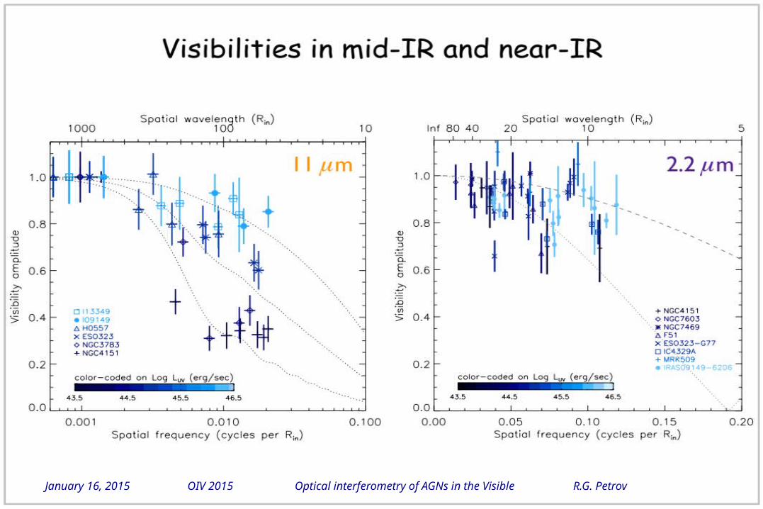
• Clumpy torus (indeed)• Near-IR sizes factor 3 smaller than anticipated; (2) • Surface emissivity ~0.3 pointing to high emissivity (>0.1) = large grains• Bulk of mid-IR emission (>50-80%) comes from polar region, which has
not been expected.• This seems luminosity dependent: higher polar excess at low
luminosity: Luminosity dependent structure• Direct distance measurements
– but morphology dependent
• MATISSE will make images of an handful of QSOs
January 16, 2015 OIV 2015 Optical interferometry of AGNs in the Visible R.G. Petrov

Size of dust torus
28January 16, 2015 OIV 2015 Optical interferometry of AGNs in the Visible R.G. Petrov
Kishimoto, A&A, 2011

Conclusion for IR VLTI observations
• Optical interferometry could provide enough measures by 2020 to:• Measure the morphological parameters of 60 QSOs and Sy1 AGNs
– angular size, radial distribution of clouds, latitudinal distribution of clouds, local-to-global velocity ratio, radial-to-rotation ratios,
– study this parameters as a function of luminosity, RM key measures, light curve parameters
• Calibrate Mass-Luminosity and Size-Luminosity laws• Calibrate GAIA morphology dependent biases on QSOs• Masses and direct distances from GAIA luminosity and variability
measures.
January 16, 2015 OIV 2015 Optical interferometry of AGNs in the Visible R.G. Petrov 29

Observing BLRs with MATISSE
January 16, 2015 OIV 2015 Optical interferometry of AGNs in the Visible R.G. Petrov 30
Biased Reverberation Mapping of 3C273
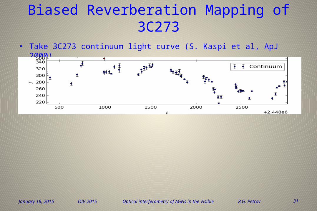
• Take 3C273 continuum light curve (S. Kaspi et al, ApJ 2000)
January 16, 2015 OIV 2015 Optical interferometry of AGNs in the Visible R.G. Petrov 31

Biased Reverberation Mapping of 3C273
• Take 3C273 continuum light curve (S. Kaspi et al, ApJ 2000)• Produce 500 interpolations of this light curve (damped random walk model, Y. Zu et
al, ApJ 2011)
January 16, 2015 OIV 2015 Optical interferometry of AGNs in the Visible R.G. Petrov 32

Biased Reverberation Mapping of 3C273
• Take 3C273 continuum light curve (S. Kaspi et al, ApJ 2000)• Produce 500 interpolations of this light curve (damped random walk model, Y. Zu et
al, ApJ 2011)• For each continuum light curve, produce a line light curve, with time delay tin.
January 16, 2015 OIV 2015 Optical interferometry of AGNs in the Visible R.G. Petrov 33
Biased Reverberation Mapping of 3C273
• Take 3C273 continuum light curve (S. Kaspi et al, ApJ 2000)• Produce 500 interpolations of this light curve (damped random walk model, Y. Zu et
al, ApJ 2011)• For each continuum light curve, produce a line light curve, with a time delay tin.
• Compute the RM cross-correlation function, deduce a measured time delay tout and plot tout = f(tin).
January 16, 2015 OIV 2015 Optical interferometry of AGNs in the Visible R.G. Petrov 34

Last minute results
January 16, 2015 OIV 2015 Optical interferometry of AGNs in the Visible R.G. Petrov 35
• Differential phase on longest baselines
• Broad, asymmetric, blue shifted signal– BLR or dust clouds anisotropy
makes a symmetric signal
• Need model of BLR – partially shielded by torus– with a slight outflow– ...
Dust tori interferometry
36January 16, 2015 OIV 2015 Optical interferometry of AGNs in the Visible R.G. Petrov

Steeper / Shallower structure
37January 16, 2015 OIV 2015 Optical interferometry of AGNs in the Visible R.G. Petrov
Discussion
38
• The high L (or high Eddington ratio) sources seem to have a much more stepper dust distribution
• Possible explanation: radiation pressure on dust– Possible anisotropic illumination
• anisotropy of acc. disk (Netzer 1985; Kawaguchi 2011)• Shielding in equatorial plane
– Interferometric measurements of elongation in the polar direction (polarization direction) (Hoenig, 2012, 2013)
• Dusty wind ?
– There are models for efficiently blown away dusty gas (e.g. Semenov 2003)
• High L: polar region cleared by radiation pressure• Low L: polar dusty wind
January 16, 2015 OIV 2015 Optical interferometry of AGNs in the Visible R.G. Petrov

January 16, 2015 OIV 2015 Optical interferometry of AGNs in the Visible R.G. Petrov 39
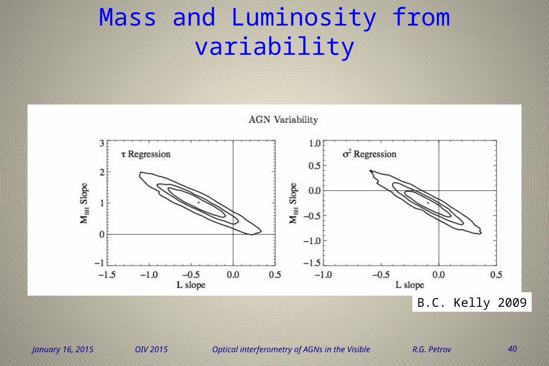
Mass and Luminosity from variability
January 16, 2015 OIV 2015 Optical interferometry of AGNs in the Visible R.G. Petrov 40
B.C. Kelly 2009

AMBER+ is a new observation modeand 2DFT data reductionthat works for SNR per channel and per frame <<1=> gain > 2 magnitudes
41
K=4 K=8.5 K=10
January 16, 2015 OIV 2015 Optical interferometry of AGNs in the Visible R.G. Petrov
3C273 fringe peaks (10 s)

First results, first problems
• Differential visibility– Vdiff(50m) =0.98±0.03
– Vdiff(80m) =0.94±0.04
– Vdiff(125m)=0.92±0.04
• Differential phase– Fdiff <0±2°
• RBLR> 0.5 mas, i.e. > 1500 ld
• Results show artifacts
January 16, 2015 OIV 2015 Optical interferometry of AGNs in the Visible R.G. Petrov 42
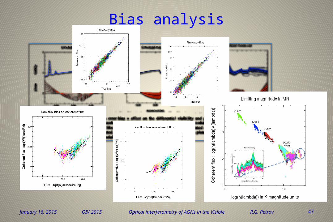
Bias analysis
January 16, 2015 OIV 2015 Optical interferometry of AGNs in the Visible R.G. Petrov 43
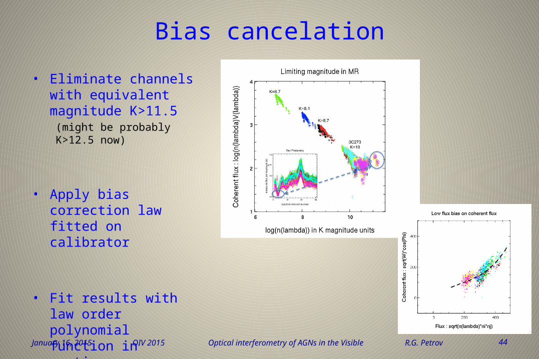
Bias cancelation
• Eliminate channels with equivalent magnitude K>11.5
(might be probably K>12.5 now)
• Apply bias correction law fitted on calibrator
• Fit results with law order polynomial function in continuum
January 16, 2015 OIV 2015 Optical interferometry of AGNs in the Visible R.G. Petrov 44

Final measures
• Differential visibility accuracy <0.01 per channel
• Visibility drops on all baselines (SNR=10 on largest baseline)
• Differential visibility drop extends over full line
• Differential phase = 0±0.5° per channel of 1250 km/s
January 16, 2015 OIV 2015 Optical interferometry of AGNs in the Visible R.G. Petrov 45
resolution=240
resolution=480

BLR structure
January 16, 2015 OIV 2015 Optical interferometry of AGNs in the Visible R.G. Petrov 46
• Flat BLRs with global velocity field seem excluded
• With such a large BLR, to cancel the differential phase, we need:
• A very small inclination– Line and visibility profile width entirely
due to local velocity– Very poor fits
• If i>10°– global velocity field large enough to
explain line width large differential phase
– need large opening angle– and/or large turbulent velocity field

Global fit
January 16, 2015 OIV 2015 Optical interferometry of AGNs in the Visible R.G. Petrov 47
• RBLR=6.26±0.1 mas– RBLR=6.26±0.1 mas
– RBLR=1880±30 ld
• Inclination not really constrained below i<15°
• Opening angle larger than 85°• Turbulent velocity field 1500
km/s• Mass little sensitive to
inclination: MBH=5.4-0.4+0.2 Msun
Conclusion and perspective on BLRs in the K band
• Our VLTI/AMBER measures on 3C273 are real• The BLR of 3C273 is much larger than the dust inner rim• The radius RBLR=6.3±1.5 mas (1850±600 ld) is much larger than RM estimate• The BLR is very close to be a sphere (w>80°)• The BLR mass estimate is 5.4±1.0 108 Msun (dominated by absolute visibility accuracy
measure)
• We are not fitting the s(l) and V(l) wings properly– work on the radial distribution of luminosity
• A better SNR would allow us to analyze the actual profiles of s(l) and V(l) • Measuring a differential phase would make a real difference• More targets...
January 16, 2015 OIV 2015 Optical interferometry of AGNs in the Visible R.G. Petrov 48