1

Role of the Non-Collinear Polarizer Layer in Spin Transfer Torque

Switching Processes

Chun-Yeol You1 and Myung-Hwa Jung2,a)

1Department of Physics, Inha University, Incheon 402-751, Korea

2Department of Physics, Sogang University, Seoul 121-742, Korea

We have recently reported that the spin transfer torque switching current density is very

sensitive to not only the junction sizes but also the exchange stiffness constants of the

free layer according to the micromagnetic simulations. The results are very complicate

and far from the macro-spin model because of the non-coherent spin switching

processes. The dependence of the switching current density on the junction sizes and the

exchange stiffness constants becomes systematic when we employ the non-collinear

polarizer layer. It is found that the non-collinear polarizer layer enhances the coherency

of the spin dynamics by breaking symmetric spin configurations.

PACS: 75.76.+j, 72.25.-b, 85.75.Dd, 75.78.Cd

a)Author to whom correspondence should be addressed. E-mail : mhjung@sogang.ac.kr

2

I. Introduction

The switching current density in the spin transfer torque magnetic random access

memory (STT-MRAM) is one of the most important key issues in the development of

the next generation non-volatile memory devices. A high switching current density

causes the reliability problem of magnetic tunneling junction (MTJ) and the size limit of

device. Therefore, there have been many approaches to reduce the switching current

density through the optimization of layer structures and magnetic properties of the

switching layer.1,2,3,4,5,6,7 Recently, we have reported that the switching current density is

very sensitive to the exchange stiffness constants8 and the lateral junction dimensions9

by micromagnetic simulations. We have also found that the switching current

dependences are unpredictably complicated,8,9 which cannot be explained with simple

model. Since the complicated spin configurations during the switching processes are

main reasons of unexpected switching current density dependences, the detail spin

configuration can be determined by the characteristic length scale of ex effA K , where

Aex is the exchange stiffness constant and Keff is an effective anisotropy energy including

demagnetization energy. When the lateral dimensions of the junction are comparable

with that characteristic length, the detail spin configuration becomes very complex.

Therefore, such unexpected switching current density dispersion with small variation of

junction sizes and fabrication conditions may act as a hurdle to commercialize the STT-

MRAM, and it is clear that more coherent spin rotation is desirable for the device

operations.

By virtue of ultrafast time resolution and nanometer scale spatial resolution of the X-

ray microscopy, it has been revealed that the complicate non-uniform modes are created

3

during the switching procedures for the 110 × 180, 110 × 150, and 85 × 135 nm2

junctions.10,11 Even though there are no vortex formations in the smaller junctions

unlike 110 × 180 nm2 junction, the switching process are always accompanied with

complex non-uniform and non-coherent spin configurations. It has been known that the

“non-collinear polarizer layer”, the magnetization directions between polarizer layer and

switching layer are non-collinear, leads better coherent spin rotations.12,13 It has been

shown that the non-collinear polarizer layer leads more coherent spin rotations by

experiments and micromagnetic simulations for the 60 x 130 nm2 junctions.13 We also

demonstrated that the non-collinear polarizer layer structure can reduce the switching

current density significantly (40 %) even for the smaller junction size (60 x 40 nm2).14

Based on our previous work about the non-collinear polarizer layer, in this work, we

would like discuss more details of the role of the non-collinear polarizer layer. We found

that the non-collinear polarizer layer plays important roles not only in the reduction of

the switching current density, but also in weak and predictable dependences of the

exchange stiffness constants and the junction sizes. Therefore, the non-collinear

polarizer layer structure has many advantages in the devices designs.

II. Macro-Spin Model

Figure 1 shows the MTJ structure with the non-collinear polarizer. The magnetization

of the switching layer F1 is aligned along the x axis, and the magnetization of the

polarizer layer in the SyA structure (F2/NM/F3) is aligned with an angle pθ from the x

axis. Here, I, NM, and AFM are the insulating, non-magnetic, and antiferromagnetic

layers, respectively. The direction of positive current and the axis of coordinates are also

depicted in Fig. 1. A, B, C, and D indicate local points of the switching layer, which will

4

be used later.

Let us derive the analytic expression of the switching current density with the non-

collinear polarizer layer based on the macro-spin model. The Landau-Lifshitz-Gilbert

(LLG) equation with STT term is

( ) ( )s ss eff s J s s p J s p

dm dmm H m a m m m b m mdt dt

γ α γ γ= − × + × − × × − × . (1)

Here, γ is the gyromagnetic ratio, α is the Gilbert damping constant, and 1Ja a J=

with 102p

s s

ae M d

ημ

= and J the current density (opposite to the electron flow).

,s pm and ,s pm are the unit vectors of the magnetization of switching and polarizer

layers, and effH is the effective field including external field. pη , ds , Ms, μ0, and

are the spin polarization of the polarizer layer, the thickness of the switching layer, the

saturation magnetization, the permeability of the vacuum, and the reduced Plank’s

constant, respectively. More details can be found in our previous works.14,15,16 For

simplicity, we ignore the field-like STT term by setting bJ = 0 because the overall Jc

dependence on the polarizer angle is not changed with the field-like term, as we have

already shown in our previous result.14

We repeat the standard method of spin wave excitation to find the switching current

density by using instability conditions17,18,19 with the non-collinear polarizer layer. We

assume that the initial state is ( ) ˆ0sm t x= = and ( ) ˆ ˆ0 cos sinp p pm x yθ θ= + , where

pθ is the magnetization angle of the polarizer layer from the x axis as shown in Fig. 1.

Let us define the excited non-zero x- and y-components of magnetization by STT, that is

( ),x ym tΔ . We put ( ),x ym tΔ contributions to Eq. (1), and linearize them up to the first

5

order of ( ),x ym tΔ , because they are supposed to be small. After linearizing, we obtain

two coupled differential equations of ( ),x ym tΔ . Let us put ( ), ,kt

x y x ym t m eΔ = Δ with

the simple harmonic oscillation model, here k is a complex number. With the same

procedures with previous report,6 we find following matrix equation;

( )( )cos

0cos

J p eff y x s x

yeff z x s J p

k a k H N N M mmk H N N M k a

γ θ α γ γ

α γ γ γ θ

⎛ ⎞+ + + − Δ⎛ ⎞⎜ ⎟ =⎜ ⎟⎜ ⎟ Δ+ + − + ⎝ ⎠⎝ ⎠

, (2)

where , , andx y zN N N are demagnetization factors of each direction. The determinant

of matrix must be zero in order to have non-trivial solutions. The characteristic equation

of the matrix is a quadratic equation of k, and the instability condition is

( )( )2Re[ ] 2 2 cos 01 eff y z x s J pk H N N N M aγ α θ

α⎡ ⎤= − + + − + >⎣ ⎦+

. (3)

Then, we find ( )c pJ θ as follows;

( )( )1cos cos 2 2J p p eff y z x sa a J H N N N Mθ θ α= < − + + − , (4)

( ) ( )( ) 0

1

2 2cos cos

cc p eff y z x s

p p

JJ H N N N Ma

αθθ θ

< − + + − = . (5)

Here, Jc0 is the switching current density with the collinear polarizer layer ( 0pθ = ) in

a normal STT structure. From these results, we can claim that the switching current

density of the non-collinear polarizer is inversely proportional to the cosine.

Furthermore, we also numerically solve the LLG equation with the macro-spin model,6

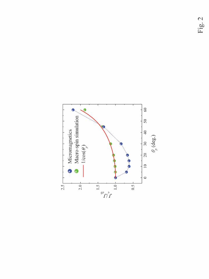
and the results show the inverse cosine dependence as shown in Fig. 2 with Eq. (5). In

Fig. 2, we also depict the normalized switching current densities from previous

micromagnetic simulation result.14

6

III. Micromagnetic Simulations

The micromagnetic simulations are performed by using the public domain

micromagnetic simulator, Object-Oriented MicroMagnetic Framework (OOMMF)20

with the public STT extension module.15 A typical STT-MRAM structure21 in Fig. 1 is

fully considered in micromagnetic simulations. The saturation magnetization Ms and

thicknesses of the F1, F2, and F3 layers are 1.3×106 A/m and 2 nm, respectively. The

thicknesses of the NM and I layers are 1 nm. The cross-section of the nano-pillar is an

ellipse of 60×40 nm2(or varied from 40 to 120 nm × 30 nm in Sec. V), with a mesh

size of 1×1×1 nm3. For simplicity, the crystalline anisotropy energy is not considered in

this study. Aex was set as 2.0×10-11 J/m (or varied from 0.5 to 3.0×10-11 J/m in Sec. V),

and the Gilbert damping constants α is 0.02. The exchange bias field of 4×105 A/m is

assigned to a pπ θ+ direction from the long axis of the ellipse (+x direction) for the F3

layer. Due to the exchange bias, the magnetization direction of the F3 layer prefers the

pπ θ+ direction. Because we design a strong antiferromagnetic interlayer exchange

coupling (-1.0×10-3 J/m2) between the F2 and F3 layers to mimic a typical SyF structure,

the magnetization direction of the F2 layer is pθ as shown in Fig. 1. More details of the

micromagnetic simulation results have been reported in Ref. [14].

IV. Reduction of the Switching Current Density

We depict the results of the switching current densities of the micromagnetic

simulation, Eq.(5), and the numerical simulations of the macro-spin model in Fig. 2.

7

Here, the numerical simulation of the macro-spin means the switching current density is

obtained by numerically solving LLG equations for the macro-spin. In Fig. 2, all

switching current densities are normalized with the value of the collinear polarizer layer

( pθ =0). Therefore, it must be mentioned that values Jc0 are different for three cases; Jc0

= 2.7×1011 A/m2 for the micromagnetic simulation, Jc0 = 1.84×1011 A/m2 for the

analytic macro-spin model Eq. (5), and Jc0 = 2.17×1011 A/m2 for the numerical macro-

spin calculation, respectively. The reason of such discrepancy will be discussed later.

Surprisingly, the macro-spin model and micromagnetic simulation results are

opposite for small pθ as shown in Fig. 2. The Eq. (5) and the numerical macro-spin

model calculations imply that the non-collinear polarizer will increase the switching

current density. However, the micromagnetic simulation results show noticeable

reduction of the switching current density. The main reason is that the macro-spin model

is failed for the collinear polarizer layer due to the non-uniform spin configuration

during switching processes. For the non-collinear polarizer case, the switching

processes occur with the coherent spin rotation which is well described by the macro-

spin model. Therefore, the reduction of the switching current density for the non-

collinear polarizer is mainly due to the enhanced coherent spin rotation.12,13

In order to get deep insight of the switching process, we take snapshots of the spin

configuration of the switching layer as shown in Figs. 3 and 4 for collinear ( 0pθ = ) and

non-collinear ( o10pθ = ) polarizer layers, respectively. The snapshots are taken for the

switching current density of each case. We have already discussed about the detail spin

dynamics in our previous reports for the collinear polarizer case.15,16 Before the actual

switching occurs, strong spin oscillations are found at both edges, and the phases of spin

8

oscillations at both edges are opposite.9 Such asymmetric spin dynamics of both sides

are clearly shown in Fig. 3 (a) and (b). In order to check more details, Fig. 3 (e) shows

the time dependent normalized magnetization dynamics for the specific positions (A, B,

C, and D), which are defined in Fig. 1. In Fig. 3 (e), the amplitude of oscillation is the

strongest at the edge (position A), and it decreases from point A (edge) to D (center).

Even though there are strong oscillations at both edges, the effect of STT is almost

vanished at the center because of the out-of-phase STT contributions from both sides.

Therefore, spins at the center position do not oscillate till 8.0 ns. After certain time (t ~

9.0 ns in Fig. 3 (c)), spins at the center position start to move by breaking the

asymmetric spin dynamics. After breaking the asymmetric spin dynamics, the switching

is accomplished. It must be emphasized that the detail spin dynamics of the collinear

polarizer layer in the typical STT structure is far from the coherent rotation in the

macro-spin model.16

Now let us consider the non-collinear polarizer case, as shown in Figs. 4 (a)~(d). We

find that the spin oscillations are almost coherent from the beginning (Fig. 4 (a)). The

rotation angles of each spin are almost similar, and it is quite different for the collinear

polarizer case. The coherent rotation of spins is easily confirmed from Fig. 4 (e).

Contrary to the collinear polarizer case in Fig. 3 (e), the spin dynamics of each position

from A to D for the non-collinear polarizer case are almost identical and in-phased as

shown in Fig. 3 (e).

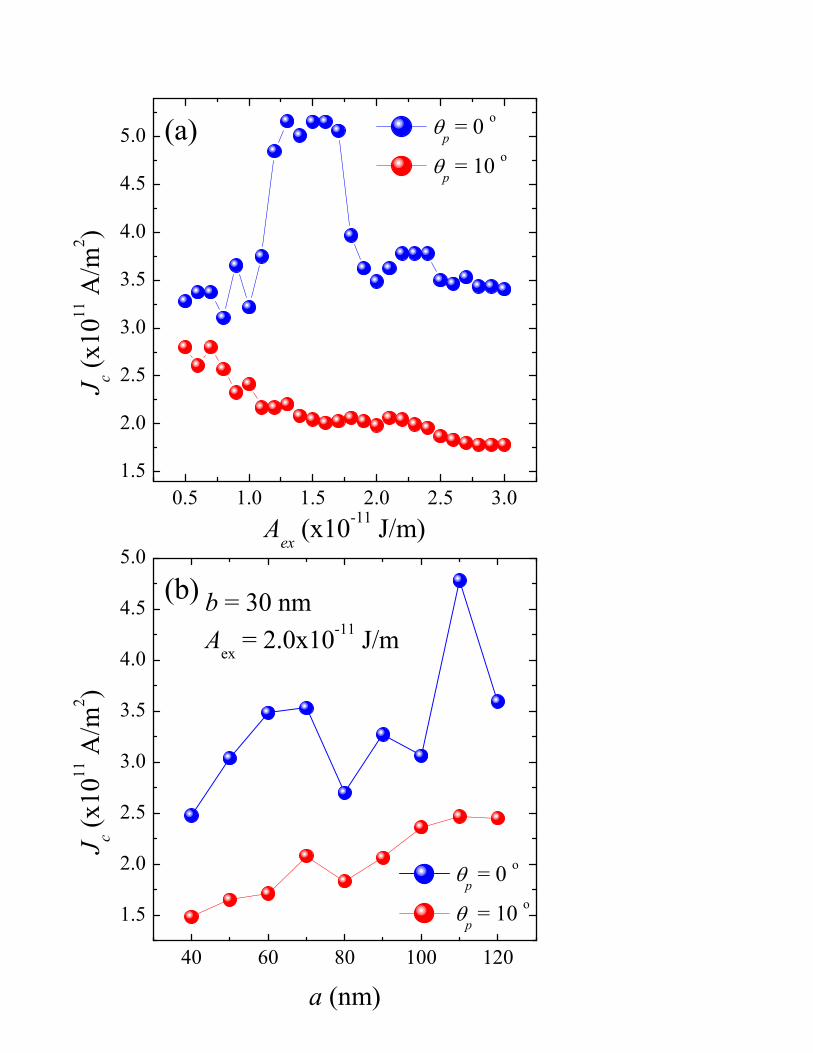
V. Dependence of the Lateral Junction Sizes and the Exchange Stiffness

Constants

Recently, we have reported that the switching current densities are very sensitive

9

function of the lateral junction sizes9 and the exchange stiffness constants, Aex.8 As

aforementioned, the switching process occurs always with the non-uniform spin

configurations, and the detail spin configurations are governed by the exchange length

and the lateral dimension of the junction. Since the macro-spin model cannot treat the

lateral junction size and the Aex,8,9 the macro-spin model failed to handle such problem

properly. Here, we recall our previous results8,9 for various Aex values of 80 × 40 nm2

junctions, and various junction sizes for the collinear ( 0pθ = ) polarizer layer. In

addition, we repeat the same simulation for the non-collinear ( o10pθ = ) polarizer layer

in Fig 5 (a) and (b). As shown in Fig. 5 (a), the switching current density dependence on

Aex is unpredictable for collinear polarizer case. It must be noted that the Aex variation

(1.0 ~ 3.0 x 10-11J/m) is realistic for CoFeB fluctuated with the fabrication conditions.22

Within these realistic variations, the switching current density varies around 60%.

However, when we consider non-collinear polarizer layer, the variation of the switching

current density shows almost monotonic decrease, and it is predictable. For the larger

Aex values, which is more likely to be macro-spin status, the switching current density

approaches to the Jc0 (= 1.84×1011 A/m2) value based on the analytic macro-spin model

with increasing Aex.

In Fig. 5 (b), we fix Aex = 2.0×10-11 J/m and short axis of the ellipse, b = 30 nm, and

varies the long axis of the ellipse, a, from 40 to 120 nm. The collinear polarizer shows

overall increase, but the data is strongly scattered so that it is not easy to say general

trend. However, when we consider the non-collinear polarizer, the dependence is

monotonically increased with small deviation. Such predictable behavior implies that

more coherent spin switching is insensitive on the lateral dimension of the junction and

10

Aex, because non-uniform spin configuration is not involved in these cases.

VI. Conclusion

In conclusion, we investigate the role of the non-collinear polarizer layer in the

typical STT structure. Based on our micromagnetic simulations, we can claim that the

realistic switching process is far from the macro-spin model in a typical STT structure

with the collinear polarizer layer. In contrast to the macro-spin model, the important

switching process always involves non-uniform and non-coherent spin rotation for the

collinear polarizer. Such non-coherent switching can be suppressed effectively with the

non-collinear polarizer layer by breaking the asymmetric spin dynamics, and it leads

conspicuous switching current density reduction. Furthermore, unpredictable and very

sensitive dependence of the switching current density on the lateral junction sizes and

the exchange stiffness constants changes to the weak and monotonic dependences.

Acknowledgements

This work was supported by the NRF funds (Grant Nos. 2010-0023798 and 2010-

0022040, Nuclear R&D Program 2012M2A2A6004261) of the MEST of Korea, and by

the IT R&D program of MKE/KEIT (10043398).

11

References

1 T. Ochiai, Y. Jiang, A. Hirohata, N. Tezuka, S. Sugimoto, K. Inomata, Appl. Phys.

Lett. 86, 242506 (2005).

2 J. Hayakawa, S. Ikeda, Y. M. Lee, R. Sasaki, T. Meguro, F. Matsukura, H. Takahashi,

and H. Ohno, Jpn. J. Appl. Phys. 45, L1057 (2006).

3 M. Ichimura, T. Hamada, H. Imamura, S. Takahashi, and S. Maekawa, J. Appl. Phys.

105, 07D120 (2009).

4 C.-T. Yen, W.-C. Chen, D.-Y. Wang, Y.-J. Lee, C.-T. Shen, S.-Y. Yang, C.-H. Tsai, C.-

C. Hung, K.-H. Shen, M.-J. Tsai, and M.-J. Kao, Appl. Phys. Lett. 93, 092504 (2008).

5 K. Lee, W.-C. Chen, X. Zhu, X. Li, and S.-H. Kang, J. Appl. Phys. 106, 024513

(2009).

6 C.-Y. You, J. Appl. Phys. 107, 073911 (2010): C.-Y. You, Curr. Appl. Phys. 10, 952

(2010).

7 S.-C. Oh, S.-Y. Park, A. Manchon, M. Chshiev, J.-H. Han, H.-W. Lee, J.-E. Lee, K.-T.

Nam, Y. Jo, Y.-C. Kong, B. Dieny, and K.-J. Lee, Nat. Phys. 5, 898 (2009).

8 C.-Y. You, Appl. Phys. Exp. 5, 103001 (2012).

9 C.-Y. You and M.-H. Jung, J. Appl. Phys. 113, 073904 (2013).

10 Y. Acremann, J. P. Strachan, V. Chembrolu, S. D. Andrews, T. Tyliszczak, J. A.

Katine, M. J. Carey, B. M. Clemens, H. C. Siegmann, and J. Stöhr, Phys. Rev. Lett.

96, 217202 (2006).

11 J. P. Strachan, V. Chembrolu, Y. Acremann, X.W. Yu, A. A. Tulapurkar, T. Tyliszczak,

J. A. Katine, M. J. Carey, M. R. Scheinfein, H. C. Siegmann, and J. Stöhr, Phys. Rev.

Lett. 100, 247201 (2008)..

12

12 I. N. Krivorotov, N. C. Emley, J. C. Sankey, S. I. Kiselev, D. C. Ralph, and R. A.

Buhrman, Science 307, 228 (2005).

13 G. Finocchio, I. N. Krivorotov, L. Torres, R. A. Buhrman, D. C. Ralph, and B.

AzzerboniI. Phys. Rev. B 76, 174408 (2007).

14 C.-Y. You, Appl. Phys. Lett. 100, 252413 (2012).

15 C.-Y. You, J. of Magnetics, 17, 73 (2012).

16 C.-Y. You, Appl. Phys. Exp. 5, 103001 (2012).

17 J. Z. Sun: Phys. Rev. B 62 (2000) 570.

18 S. M. Rezende, F. M. de Aguiar, and A. Azevedo, Phys. Rev. Lett. 94, 037202 (2005).

19 J. Grollier, V. Cros, H. Jaffrès, A. Hamzic, J. M. George, G. Faini, J. Ben Youssef, H.

Le Gall, and A. Fert, Phys. Rev. B 67, 174402 (2003).

20 M. J. Donahue and D. G. Porter: OOMMF User's Guide, Ver. 1.0, Interagency Report

NISTIR 6376, NIST, USA (1999).

21 M.-H. Jung, S. Park, C.-Y. You, and S. Yuasa, Phys. Rev. B 81, 134419 (2010): C.-Y.

You, J. Yoon, S.-Y. Park, S. Yuasa, M.-H. Jung, Cur. Appl. Phys. 11, e92 (2011).

22 Jaehun Cho, Jinyong Jung, Ka-Eon Kim, Sang-Il Kim, Seung-Young Park, Myung-

Hwa Jung, and Chun-Yeol You, J. Mag. Mag. Mat. 339, 36 (2013).

13

Figure Captions

Fig. 1 MTJ structure with non-collinear polarizer layer. F1,2,3 are the ferromagnetic

layers, and I, NM, and AFM are the insulating, non-magnetic, antiferromagnetic layers,

respectively. The positive current is defined from the bottom to top electrodes, and x-

axis is the long axis of the ellipse. The average magnetization angel of the polarizer

layer, pθ , are also depicted. A, B, C, and D indicate the specific positions of the

switching layer.

Fig. 2 Normalized switching current density obtained from the micromagnetic

simulations, macro-spin models, and Eq. (5) as a function of the polarizer layer

magnetization direction, pθ . Here, Jc0 = 2.7×1011 A/m2 for micromagnetic simulation,

Jc0 = 1.84×1011 A/m2 for analytic macro-spin model, and Jc0 = 2.17×1011 A/m2 for

numerical macro-spin simulation, respectively.

Fig. 3 Snapshots of spin configurations of the switching layer with the collinear

( 0pθ = ) polarizer layer at specific time with the switching current density. (a) t = 6.44

ns, (b) t = 6.51 ns, (c) t = 8.99 ns, and (d) t = 9.36 ns. (e) Time dependent normalized

magnetization at specific positions (A, B, C, and D), and total magnetization with the

collinear polarizer layer.

Fig. 4 Snapshots of spin configurations of the switching layer with the non-collinear

( o10pθ = ) polarizer layer at specific time with the switching current density. (a) t = 4.13

ns, (b) t = 6.00 ns, (c) t = 6.13 ns, and (d) t = 9.60 ns. (e) Time dependent normalized

14

magnetization at specific positions (A, B, C, and D), and total magnetization with the

non-collinear polarizer layer.

Fig. 5 Switching current density as a function of (a) the exchange stiffness constant, Aex,

for the 80 x 40 nm2 junctions, (b) the long axis of the ellipse with 30-nm short axis and

Aex = 2.0 x 10-11 J/m. The blue and red circles represent the collinear ( o0pθ = ) and non-

collinear ( o10pθ = ) polarizer layers, respectively.

F 1 I F 2

NM

F 3

A

FM

curr

ent

J >

0

x

z

F 1

F 2

F 3

p

A B

C D

Fig.

1

(b) t

=6.

00 n

s

(c) t

=6.

13 n

s (d

) t =

9.60

ns

(a) t

=4.

13 n

s

Fig.

4

A B

C D

0.0

2.0

4.0

6.0

8.0

10.0

12.0

0246810

DTota

l

C B

Mx (arb. unit)

t (ns

)

A(e)