©Rohde & Schwarz; Know your jitter when debugging

White paper | Version 01.00

KNOW YOUR JITTER WHEN DEBUGGINGVerifying signal integrity in high-speed digital design

22

CONTENTSIntroduction ..........................................................................................................................................................3

Rohde & Schwarz releases new oscilloscope tool designed to decompose jitter ...........................................4

Signal model based approach to joint jitter and noise decomposition ...........................................................7

Verifying the true jitter performance of clocks in high-speed digital designs ..............................................27

Verifying the clock source .................................................................................................................................30

The terms HDMI and HDMI High-Definition Multimedia Interface, and the HDMI Logo are trademarks or registered trademarks of HDMI Licensing, LLC in the United States and other countries.

Rohde & Schwarz White paper | Know your jitter when debugging 3

INTRODUCTIONJitter is a fact of life in test and measurement. No matter how cleverly you craft your circuit, no matter how many precautions you take in every step of the design process to minimize noise sources, jitter will appear in your clock signal or serial bus data, regardless.

For some engineers, jitter may not cast a long shadow over their designs. For others, however – often those working with very high-precision, high-speed applications – it is an extremely important consideration. Whether you are designing for arbitrary wave-form generation, data transmission equipment, or medical imaging devices, reducing the uncertainty of where edge crossings occur can be crucial to understanding how jitter affects a system.

Modern tools offer features that make jitter analysis significantly easier than in decades past. Not only are there more intuitive user interfaces on test equipment but there are also increasingly sensitive and accurate analysis tools.

This white paper is designed to provide you with a toolbox of educational content on how to look for, assess, and address jitter in your signal verification tasks, such as meeting your specified jitter budget.

You will find three easy-to-parse resources which present real-world scenarios that first pose an everyday engineering task and then deliver background information and recom-mended test and measurement solutions – all in a bite-sized format.

You will also find a fascinating whitepaper wherein experts from Rohde & Schwarz argue that TIE (time interval error) data alone is not enough for decomposing signals in modern, demanding high-speed serial signal applications and propose a new parametric signal model.

Finally, you will find an announcement of one of the latest Rohde & Schwarz oscilloscope tools designed to specifically help engineers better analyze jitter on the job.

We hope this set of articles serves the EE community well when jitter matters most.

Hannah DeTavisSenior Editor of All About Circuits

4

ROHDE & SCHWARZ RELEASES NEW OSCILLOSCOPE TOOL DESIGNED TO DECOMPOSE JITTERWhy is jitter becoming an increasingly difficult problem to solve? Rohde & Schwarz helps designers respond to these challenges with a jitter analysis tool.

WHAT IS JITTER?Jitter, in laymen terms, is randomness in signal frequency whereby a signal source, such as a 1 kHz square wave, will not always be at 1 kHz. Some portions of the waveform will be higher than 1 kHz and others will lower than 1 kHz.

This variance in frequency, which changes with time, has its own frequency and altera-tions in the waveform. Those that occur at a rate greater than 10 Hz are called jitter whereas those under 10 Hz are referred to as wander. But when does jitter become a problem and what applications are most at risk?

JITTER IN COMMUNICATIONS AND DSPGenerally speaking, communications links are those most prone to jitter problems. This is because these applications must transmit data that is synchronized to a clock source. Other applications, including digital signal processors, can also experience jitter.

Why does a circuit suffer from jitter and what should designers look out for? Simply put, major issues with jitter arise when the variance in a clock signal interferes with data trans-mission timing.

If, for example, a UART port operates at 300 baud and its reference clock source is a 64 MHz crystal, then the variance from the crystal is so small (parts per million) that even the most extreme signal variance of the 64 MHz will have little effect on the 300 baud signal.

If a 300 baud UART port derives its timing from a clock source whose variance caused a UART frequency shift of 10 Hz, then suddenly the baud rate (which is now changing by ±3 %) becomes significant enough that data on the receiving end can be misinterpreted.

So, to summarise, jitter becomes a problem when variance in the frequency of the signal is significant enough to adversely affect the timing of data. Jitter does not affect data rates because of a change in frequency; the changing frequency causes the data on the receiving end to be misinterpreted.


ROHDE & SCHWARZ JITTER DECOMPOSITIONWhen determining the jitter of a system, an analysis tool that generates eye diagrams can provide great insight into the amount of jitter in a circuit and determine a safe area of operation. However, determining jitter is only the first step. The type of jitter also needs to be determined. From there, designers can figure out how to identify sources of jitter and rectify the issue if needed.

Rohde & Schwarz is responding to this conversation on jitter with its newly announced tool, R&S®RTO-K133/R&S®RTP-K133, that will be included in their oscilloscope products.

R&S®RTO-K133/R&S®RTP-K133 advanced jitter analysis option

The jitter tool not only produces the eye diagram for a signal but also separates the jitter into its individual components. These include random jitter, data-dependent jitter, and periodic jitter. Using this analysis, a designer can determine if jitter is the result of random variations in the circuit or if it is due to the interference from components when data is transmitted.

What also makes the R&S®RTO-K133/R&S®RTP-K133 tool unique is that it performs the test on the complete characteristic of the waveform under test, unlike other standard tests that only perform time interval error measurements.

OTHER JITTER INSPECTION TOOLSJitter tools are not only limited to one or two specialized oscilloscopes. Designers can find these tools from many different manufacturers. For instance, in the past, we have discussed how Rigol released an oscilloscope in 2019 called the MSO8000, which includes jitter analysis in real-time with a bandwidth of up to 2 GHz. It also produces eye diagrams.

Keysight, another company based around signal analysis, also produces jitter measuring tools. For instance, their sampling oscilloscope, the 86100C DCA-J, can perform jitter analysis between 50 Mbps to over 40 Gbps. The device, highly sensitive to intrinsic jitter, conveys jitter types and offers multiple views on the jitter data.

What makes the Rohde & Schwarz tool different is that it is incorporated into standard bench oscilloscopes whereas the Keysight 86100C DCA-J is a specialized tool.

https://www.rohde-schwarz.com/us/product/sw_rtx-k133-productstartpage_63493-732992.html#m/fb7:0

https://www.allaboutcircuits.com/news/rigols-newest-mso8000-oscilloscope-offers-2-ghza-bandwidth/

https://www.allaboutcircuits.com/news/rigols-newest-mso8000-oscilloscope-offers-2-ghza-bandwidth/

https://www.rigolna.com/MSO8000/

https://www.keysight.com/en/pd-318628-pn-86100C/infiniium-dca-j-wideband-oscilloscope-mainframe?cc=US&lc=eng

6

CONCLUSIONWhile it is clear that jitter can be highly problematic in environments with high-speed data connections, jitter can also be a problem in other digital circuitry. The ability to measure it can provide insight into the quality of a signal and the amount of noise present.

Being able to differentiate the type of jitter can drastically reduce debug time by helping to identify which components in a circuit are causing the jitter.


SIGNAL MODEL BASED APPROACH TO JOINT JITTER AND NOISE DECOMPOSITION

1 INTRODUCTIONThe identification of jitter and noise sources is critical when debugging failure sources in the transmission of high-speed serial signals. With ever increasing data rates accompa-nied by decreasing jitter budgets and noise margins, managing jitter and noise sources is of utmost relevance. Methods for decomposing jitter have matured considerably over the past 20 years; however, they are mostly based on time interval error (TIE) measurements alone [1, 2]. This TIE-centric view discards a significant portion of the information present in the input signal and thus limits the decomposition accuracy.

The field of jitter separation was conceived in 1999 by M. Li et al. with the introduction of the Dual-Dirac method [3]. The Dual-Dirac method was augmented and improved over the next two decades. Originally, it was meant to isolate deterministic from random jitter components based on the probability density of the input signal’s TIEs. It uses the fact that deterministic and random jitter are statistically independent and that determin-istic jitter is bounded in amplitude, while random jitter is generally unbounded. Three years later, M. Li et al. reported that their Dual-Dirac method systematically overestimates the deterministic component [4]. Despite this flaw, modelling jitter using the Dual-Dirac model has maintained significance in commercial jitter measurement solutions due to its simplicity [5].

Throughout the years, additional techniques were added to the original Dual-Dirac method to separate additional jitter sources such as intersymbol interference (ISI), peri-odic jitter (PJ) and other bounded uncorrelated (OBU) jitter. For example, PJ components can be extracted using the autocorrelation function [6] or the power spectral density [7, 8] of the TIEs, while the ISI part of deterministic jitter can be determined by averaging periodically repeating or otherwise equal signal segments [13]. Yet another method for estimating ISI makes use of the property that ISI can be approximately described as a superposition of the effect of individual symbol transitions on their respective TIE [12]. Once the probability density function of one jitter component is known, any second component can be estimated from a mix of the two by means of deconvolution approaches, as long as the components are statistically independent of each other [9, 10, 11]. Collectively, over 40 IEEE publications and more than 50 patents can be found on the topic of jitter analysis alone. Despite this, applications in industrial jitter measurements commonly use a combination of the previously described methods [14, 15, 16], all based solely on TIEs.

In this paper, we first introduce a parametric signal model for serial pulse-amplitude modulated (PAM) transmission that includes jitter and noise contributions. The key to this model is a set of step responses, which characterizes the deterministic behavior of the transmission system, similar to the impulse response in traditional communica-tions systems. Based on the signal model, we propose a joint jitter and noise analysis framework that takes into account all information present in the input signal. This frame-work relies on a joint estimation of model parameters, from which we readily obtain the commonly known jitter and noise components. Therefore, we provide a single

8

mathematical base yielding the well-known jitter/noise analysis results for PAM signals and thus a consistent impairment analysis for high-speed serial transmission systems.

Additionally, we provide deep system insight through the introduction of new measure-ments, such as what-if signal reconstructions based on a subset of the underlying impairments. These reconstructions enable the visualization of eye diagrams for a selec-tion of jitter/noise components, thereby allowing informed decisions about the relevance of the selected components. Similarly, we determine selective symbol error rate (SER) and bit error rate (BER) extrapolations to allow fast calculation of (selective) peak-to-peak jitter and noise amplitudes at low error rates. The proposed framework is inherently able to perform accurate measurements even using relatively short input signals. This is due to the significant increase in information extracted from the signal. Furthermore, our approach has no requirements regarding specific input symbol sequences, such as predefined compliance patterns. On the contrary, the random or scrambled input data typically encountered in real-world scenarios is ideally suited to the framework.

2 SIGNAL MODELThe proposed joint jitter and noise analysis framework is based on a signal model for serial PAM data transmission. This model assumes the total signal, i.e. the received signal containing all components, to be

Signal Model-Based Approach to a Joint Jitter &Noise Decomposition

Abstract

I. INTRODUCTION

II. SIGNAL MODEL

y(t) =∞∑

k=−∞

∆s[k] · hsr(t− Tclk[k]− εh[k], s) + y−∞ + εv(t). (1)

hsr(t− Tclk[k]− εh[k], s) = hsr(t− Tclk[k]− εh[k], {s[k],∆s[k]}). (2)

εh[k] = εh,P [k] + εh,OBU[k] + εh,R[k] =

NP (h)−1∑l=0

Ah,l sin(2πfh,lTh,l[k] + φh,l) + εh,OBU[k] + εh,R[k] (3)

εv(t) = εv,P (t) + εv,OBU(t) + εv,R(t) =

NP (v)−1∑l=0

Av,l sin(2πfv,lt+ φv,l) + εv,OBU(t) + εv,R(t). (4)

III. JITTER AND NOISE DECOMPOSITION

A. Source and Analysis DomainsB. Decomposition Tree

yR(h)(t) =∞∑n=1

1

n!

∞∑k=−∞

∆s[k] ·∂n

∂tnhsr(t− Tclk[k], {s[k],∆s[k]}) · (−εh,R[k])

n. (5)

yR(h)(t) = −∞∑

k=−∞

∆s[k] ·∂

∂thsr(t− Tclk[k], {s[k],∆s[k]}) · εh,R[k]. (6)

(1)

Here, s denotes the vector of the transmitted PAM symbol sequence

Information Classification: General

known jitter/noise analysis results for PAM signals and thus a consistent impairment

analysis for high-speed serial transmission systems.

Additionally, we provide deep system insight through the introduction of new

measurements, such as what-if signal reconstructions based on a subset of the underlying

impairments. These reconstructions enable the visualization of eye diagrams for a selection

of jitter/noise components, thereby allowing informed decisions about the relevance of the

selected components. Similarly, we determine selective symbol error rate (SER) and bit

error rate (BER) extrapolations allowing for a fast calculation of (selective) peak-to-peak

jitter and noise amplitudes at low error rates.

The proposed framework is inherently able to perform accurate measurements even for

relatively short input signals. This is due to the significant increase in information extracted

from the signal. Furthermore, our approach has no requirements regarding specific input

symbol sequences, such as predefined compliance patterns. On the contrary, random or

scrambled input data typically encountered in real-world scenarios is ideally suited to the

framework.

2 Signal Model

The proposed joint jitter and noise analysis framework is based on a signal model for serial

PAM data transmission. This model assumes the total signal, i.e., the received signal

containing all components, to be

(1)

Here, denotes the vector of the transmitted PAM symbol sequence and

Δ 1 the symbol difference at symbol index . Moreover, ℎsr,

denotes the step response for the symbol vector at time , clk the reference clock time

at symbol index , and the initial signal value. The disturbance sources are split into

horizontal (time) and vertical (signal level) parts: is the total horizontal source

disturbance and is the total vertical source disturbance. Contrary to traditional

communication systems, we use a step response instead of an impulse response to model

the total signal. This is due to the fact that an impulse response is neither able to ensure

signal continuity under non-linear (in the signal level domain) horizontal disturbances nor

able to reproduce symbol transition asymmetries. The step response includes transmitter,

channel, and possibly receiver effects, all of which result in a data-dependent signal

disturbance, i.e., inter-symbol interference. Moreover, the step response depends on the

symbol vector in order to account for effects like symbol transition dependencies in the

transmission system. In the following, we assume the step response to depend only on the

last symbol and the last symbol transition:

and Δs[k] = s[k] – s[k – 1] the symbol difference at symbol index k. hsr (t, s) denotes the step response for the symbol vector s at time t, Tclk [k] the reference clock time at symbol index k, and y–∞ the initial signal value. The disturbance sources are split into horizontal (time) and vertical (signal level) parts: ϵh [k] is the total horizontal source disturbance and ϵv(t ) is the total vertical source disturbance. Contrary to traditional communica-tions systems, we use a step response instead of an impulse response to model the total signal. This is due to the fact that an impulse response is neither able to ensure signal continuity under nonlinear (in the signal level domain) horizontal disturbances nor able to reproduce symbol transition asymmetries. The step response includes transmitter, channel and possibly receiver effects, all of which result in a data-dependent signal disturbance, i.e. intersymbol interference. Moreover, the step response depends on the symbol vector s in order to account for effects like symbol transition dependencies in the transmission system. In the following, we assume the step response to depend only on the last symbol and the last symbol transition:


Abstract

I. INTRODUCTION

II. SIGNAL MODEL

y(t) =∞∑

k=−∞




NP (h)−1∑l=0



NP (v)−1∑l=0




yR(h)(t) =∞∑n=1

1

n!

∞∑k=−∞

∆s[k] ·∂n


n. (5)

yR(h)(t) = −∞∑

k=−∞

∆s[k] ·∂


(2)

We thus have up to NPAM ⋅ (NPAM – 1) step responses for a signal of PAM order NPAM.The total horizontal and vertical source disturbances ϵh [k] and ϵv (t ), respectively, are further decomposed as


Abstract

I. INTRODUCTION

II. SIGNAL MODEL

y(t) =∞∑

k=−∞




NP (h)−1∑l=0



NP (v)−1∑l=0




yR(h)(t) =∞∑n=1

1

n!

∞∑k=−∞

∆s[k] ·∂n


n. (5)

yR(h)(t) = −∞∑

k=−∞

∆s[k] ·∂



Abstract

I. INTRODUCTION

II. SIGNAL MODEL

y(t) =∞∑

k=−∞




NP (h)−1∑l=0



NP (v)−1∑l=0




yR(h)(t) =∞∑n=1

1

n!

∞∑k=−∞

∆s[k] ·∂n


n. (5)

yR(h)(t) = −∞∑

k=−∞

∆s[k] ·∂


(3)


The horizontal and vertical periodic components ϵh,P [k] and ϵv,P (t ), respectively, are characterized by the amplitudes Ax,l , the frequencies fx,l and the phases ϕx,l for l = 0, … , NP(x) – 1 and x = {h,v}, respectively, and Th,l [k] denotes the relevant point in time for the horizontal periodic component l at symbol k. The terms ϵh,OBU [k] and ϵv,OBU (t ) designate other bounded uncorrelated (OBU) 1) components, and the random components ϵh,R [k] and ϵv,R (t ) denote additive noise for the horizontal and vertical case, respectively. At this point, we do not impose any statistical properties on the random components.

3 JITTER AND NOISE DECOMPOSITIONAs introduced in section 2, various effects cause disturbances in transmitted data. The transmitter and the channel have the most influence on the step responses that deter-mine the data-dependent disturbance of the signal (intersymbol interference). Periodic and OBU disturbances make up the remaining deterministic and bounded components. Finally, there are random and unbounded disturbances such as thermal noise. Apart from being deterministic and bounded, very little information is available about OBU compo-nents at the receiver end. Therefore, we omit OBU components from now on. Their influence will be visible in the extracted random components.

3.1 Source and analysis domainsWith the exception of data-dependent components, all disturbances are either of hori-zontal or vertical origin. The horizontal components constituting ϵh [k] originate at the transmitter, whereas the vertical components in ϵv (t ) may also be added in the channel or at the receiver end. The data-dependent components have their origin in the combination of the data, i.e. the transmitted symbols, and the step responses that overlap to build the signal. We thus define the source domain to be either “horizontal”, “vertical” or “data”.

Analyzing the disturbances in the time domain is referred to as jitter analysis. Timing errors with respect to a reference clock signal are determined and analyzed. This is usually done by means of the TIE. However, the disturbances can also be analyzed in the signal level domain, which is referred to as noise analysis. In this case, signal level errors with respect to reference levels are determined and analyzed at symbol sampling times given by a reference clock signal. Fig. 1 depicts the definition of the TIE and the level error (LE). The choice between jitter analysis and noise analysis is a choice of the analysis domain, which we accordingly define to be either “jitter” or “noise”.

Fig. 1: TIE and LE definition

Clock time

Transition point

Sampling time

Threshold level

Reference level

Signal levelLE

TIE

1) The word “other” in OBU refers to the nonperiodicity of the disturbance and the word “uncorrelated” to the nonexistence of any correlation between the disturbance and the symbol sequence.

10

3.2 Decomposition treeThe decomposition tree of total jitter and total noise is depicted in Fig. 2. It is important to remember that, as shown in Fig. 2, horizontal disturbances also have an influence in the noise domain and vertical disturbances in the jitter domain. Thus no matter whether a jitter or a noise analysis is performed, all disturbance components need to be accounted for, i.e. for any analysis domain, all source domains are relevant. Moreover, it is generally not possible to directly map properties in a source domain to measurements in an anal-ysis domain. Consider, e.g. the case of the horizontal random source disturbance ϵh,R [k] only. Its effect on the signal level and thus the noise domain can be described by a Taylor series of ϵh,R [k] around the mean. For the zero-mean case, we obtain


Abstract

I. INTRODUCTION

II. SIGNAL MODEL

y(t) =∞∑

k=−∞




NP (h)−1∑l=0



NP (v)−1∑l=0




yR(h)(t) =∞∑n=1

1

n!

∞∑k=−∞

∆s[k] ·∂n


n. (5)

yR(h)(t) = −∞∑

k=−∞

∆s[k] ·∂


(4)

The first-order approximation of equation (4) is given by


Abstract

I. INTRODUCTION

II. SIGNAL MODEL

y(t) =∞∑

k=−∞




NP (h)−1∑l=0



NP (v)−1∑l=0




yR(h)(t) =∞∑n=1

1

n!

∞∑k=−∞

∆s[k] ·∂n


n. (5)

yR(h)(t) = −∞∑

k=−∞

∆s[k] ·∂


(5)

We recognize that the horizontal random source disturbances are transformed to the noise domain in a nonlinear manner that depends on the step responses and their deriva-tives 2). Moreover, the inverse step of determining the source disturbance based on the noise disturbance is nontrivial.

Fig. 2: Jitter and noise decomposition treea) Jitter analysis

Random horizontal jitter RJ(h)

Random verticaljitter RJ(v)

Random jitter RJ

Periodic horizontal jitter PJ(h)

Periodic vertical jitter PJ(v)

Periodic jitter PJ

Data-dependent jitter DDJ

Deterministic jitter DJ

Total jitter TJ

Unbounded

Bounded

Jitter analysis

Noise analysis

Random horizontal noise RN(h)

Random verticalnoise RN(v)

Random noise RN

Periodic horizontal noise PN(h)

Periodic vertical noise PN(v)

Periodic noise PN

Data-dependent noise DDN

Deterministic noise DN

Total noise TN

Unbounded

Bounded2) For jointly stationary ϵh,R [k] and s [k], and Tclk [k] = kTs with the constant symbol period Ts, the first-order approximation

(5) is cyclostationary. Moreover, for PAM signals of order NPAM > 2 and Gaussian distributed ϵh,R [k], ỹR(h)(t ) is not Gaussian distributed since the symbol difference Δs [k] can take on values with different amplitudes.


Fig. 2: Jitter and noise decomposition tree b) Noise analysis

Random horizontal jitter RJ(h)

Random verticaljitter RJ(v)

Random jitter RJ

Periodic horizontal jitter PJ(h)

Periodic vertical jitter PJ(v)

Periodic jitter PJ

Data-dependent jitter DDJ

Deterministic jitter DJ

Total jitter TJ

Unbounded

Bounded

Jitter analysis

Noise analysis

Random horizontal noise RN(h)

Random verticalnoise RN(v)

Random noise RN

Periodic horizontal noise PN(h)

Periodic vertical noise PN(v)

Periodic noise PN

Data-dependent noise DDN

Deterministic noise DN

Total noise TN

Unbounded

Bounded

4 JOINT JITTER AND NOISE ANALYSIS FRAMEWORKWe propose a framework that encompasses a joint jitter and noise analysis and is based on the signal model introduced in section 2. Contrary to state-of-the-art methods, which transition from a signal to a TIE representation as a first step, our approach is based directly on the total signal. It thus does not discard any information present in the (total) signal by using a condensed representation like TIEs do. The core of our framework operates independently of the analysis domain (jitter or noise) and considers all source domains (horizontal, vertical and data). The jitter and noise results are derived from a joint set of estimated model parameters.

Conceptually, the first step of the framework is to recover a clock that makes it possible to decode, i.e. recover, the data symbols. Based on the recovered clock signal and the decoded symbols, a joint estimation of model parameters is performed. Specifically, a coarse, partly spectrum based estimator recovers rough estimates of the frequencies and phases of the vertical periodic components as well as their number. These are then used for a fine, least-squares estimator that jointly determines the step responses and the peri-odic vertical components. The horizontal periodic components are similarly estimated. These estimates, along with the recovered symbols and clock, allow synthesis of signals with only selected disturbance components, e.g. the data-dependent signal. We then use the total and synthesized signals to transition to the analysis domains and calculate jitter and noise values, i.e. TIE and LE values, respectively. Fig. 3 shows a block diagram of the framework.

12

Fig. 3: Joint jitter and noise analysis framework

Jitter analysis

TIE

LE

Signal synthesisEstimation: step responsesand periodic components

Clock and data recovery

Noise analysis

SYNTH_DDEST_SR_PVDECODECLK_REC

Coarse estimation Fine estimation

SYNTH_PV

SYNTH_DDEST_PHEST_PH_COARSE

EST_PV_COARSE

SIGDD

SIGP(v)

SIGDD+P(h)

SIGT

TIEP(h)+R

TIEX

LEX

4.1 Estimation of model parametersThe fine estimator that performs a joint estimation of the model parameters is at the core of the framework and is derived as follows. First, we need to treat the remaining hori-zontal disturbances ϵh, rem[k] as additive noise for the estimator. Their influence in the signal level domain is quantified as in (5) by linearizing (1) with respect to ϵh, rem[k]:

IV. JOINT JITTER AND NOISE ANALYSIS FRAMEWORK

A. Estimation of Model Parameters

yh,rem(t) ≈ yh,rem(t) = −∞∑

k=−∞

∆s[k] · h(t− Tclk[k], {s[k], ∆s[k]}) · εh,rem[k] (7)

εv,P (t) ≈ yP (v)(t) =

NP (v)−1∑l=0

Av,l sin(2πfv,lt+ φv,l) + Av,l(∆f,v,l2πt+∆φ,v,l) cos(2πfv,lt+ φv,l) (8)

y(t) ≈ y(t) =∞∑

k=−∞

∆s[k] · hsr(t− Tclk[k], {s[k], ∆s[k]}) + y−∞ + yP (v)(t) + εv,R(t) + yh,rem(t). (9)

x =

hsr

y−∞p

= A+y (10)

yDD(t) =∞∑

k=−∞

∆s[k] · hsr(t− Tcdr[k], ∆s[k]) + y−∞ (11)

yP (v)(t) =

NP (v)−1∑l=0

Av,l sin(2πfv,lt+ φv,l). (12)

Tsig,T [k]− Tsig,DD+P (v)[k] (13)

B. Analysis Domains

TIEX [k] = Tsig,X [k]− Tcdr[k] (14)

TIET [k] = TIED[k] + TIER[k] (15)TIEDD+P (h)[k] = TIEDD[k] + TIEP (h)[k] (16)TIEDD+P (v)[k] = TIEDD[k] + TIEP (v)[k] (17)

TIED[k] = TIEDD[k] + TIEP [k]. (18)

LEX [k] = VX [k]− Vref[k] (19)

LET [k] = LED[k] + LER[k] (20)

(6)

where š [k] is the decoded symbol, Δs [k] the corresponding symbol difference, h( t, š [k],




k=−∞


εv,P (t) ≈ yP (v)(t) =

NP (v)−1∑l=0


y(t) ≈ y(t) =∞∑

k=−∞


x =

hsr

y−∞p

= A+y (10)

yDD(t) =∞∑

k=−∞

∆s[k] · hsr(t− Tcdr[k], ∆s[k]) + y−∞ (11)

yP (v)(t) =

NP (v)−1∑l=0



B. Analysis Domains






s [k] ) the impulse response, and Τclk [k] an estimated clock time.

By further approximating the vertical sinusoidal components, we obtain




k=−∞


εv,P (t) ≈ yP (v)(t) =

NP (v)−1∑l=0


y(t) ≈ y(t) =∞∑

k=−∞


x =

hsr

y−∞p

= A+y (10)

yDD(t) =∞∑

k=−∞

∆s[k] · hsr(t− Tcdr[k], ∆s[k]) + y−∞ (11)

yP (v)(t) =

NP (v)−1∑l=0



B. Analysis Domains






(7)

with the frequencies fv,l = ƒv,l + Δf,v,l and the phases ϕv,l = ϕv,l + Δϕ,v,l split into coarse and remaining parts for l = 0, … , NP(v) – 1. This yields the following approximation of the total signal:




k=−∞


εv,P (t) ≈ yP (v)(t) =

NP (v)−1∑l=0


y(t) ≈ y(t) =∞∑

k=−∞


x =

hsr

y−∞p

= A+y (10)

yDD(t) =∞∑

k=−∞

∆s[k] · hsr(t− Tcdr[k], ∆s[k]) + y−∞ (11)

yP (v)(t) =

NP (v)−1∑l=0



B. Analysis Domains






(8)

The coarse estimates and the above approximations can be used to perform a (fine) joint least-squares estimation of the step responses and the vertical periodic components:




k=−∞


εv,P (t) ≈ yP (v)(t) =

NP (v)−1∑l=0


y(t) ≈ y(t) =∞∑

k=−∞


x =

hsr

y−∞p

= A+y (10)

yDD(t) =∞∑

k=−∞

∆s[k] · hsr(t− Tcdr[k], ∆s[k]) + y−∞ (11)

yP (v)(t) =

NP (v)−1∑l=0



B. Analysis Domains






(9)

with the estimate vector x containing the Nsr estimates of the step responses in the vector hsr , the initial signal value estimate




k=−∞


εv,P (t) ≈ yP (v)(t) =

NP (v)−1∑l=0


y(t) ≈ y(t) =∞∑

k=−∞


x =

hsr

y−∞p

= A+y (10)

yDD(t) =∞∑

k=−∞

∆s[k] · hsr(t− Tcdr[k], ∆s[k]) + y−∞ (11)

yP (v)(t) =

NP (v)−1∑l=0



B. Analysis Domains






, and the estimates of the frequencies, phases, and amplitudes of the vertical periodic components in the vector p.


The matrix A+ is the pseudoinverse of the observation matrix and the vector y contains samples of the total signal. Based on these estimates and the recovered (or input) clock signal Τcdr [k], the data-dependent (DD) and the periodic vertical (P(v)) signals can be synthesized as




k=−∞


εv,P (t) ≈ yP (v)(t) =

NP (v)−1∑l=0


y(t) ≈ y(t) =∞∑

k=−∞


x =

hsr

y−∞p

= A+y (10)

yDD(t) =∞∑

k=−∞

∆s[k] · hsr(t− Tcdr[k], ∆s[k]) + y−∞ (11)

yP (v)(t) =

NP (v)−1∑l=0



B. Analysis Domains









k=−∞


εv,P (t) ≈ yP (v)(t) =

NP (v)−1∑l=0


y(t) ≈ y(t) =∞∑

k=−∞


x =

hsr

y−∞p

= A+y (10)

yDD(t) =∞∑

k=−∞

∆s[k] · hsr(t− Tcdr[k], ∆s[k]) + y−∞ (11)

yP (v)(t) =

NP (v)−1∑l=0



B. Analysis Domains






(10)

The horizontal periodic components are estimated in a two-step approach as above. More precisely, the estimation is based on the time difference




k=−∞


εv,P (t) ≈ yP (v)(t) =

NP (v)−1∑l=0


y(t) ≈ y(t) =∞∑

k=−∞


x =

hsr

y−∞p

= A+y (10)

yDD(t) =∞∑

k=−∞

∆s[k] · hsr(t− Tcdr[k], ∆s[k]) + y−∞ (11)

yP (v)(t) =

NP (v)−1∑l=0



B. Analysis Domains






(11)

where Τsig , T [k] and Τsig , DD + P(v) [k] are the level crossing time of the total and the DD + P(v) signal, respectively. Thus an estimate of the horizontal periodic (P(h)) contribu-tion to the level crossing times is obtained and the DD + P(h) signal can be synthesized.

Summarizing, we are able to synthesize signals with a subset of the underlying source disturbances. These what-if signal reconstructions allow us to provide new measure-ments with selectable disturbances. For example, it is possible to construct an eye diagram with data disturbances and chosen periodic disturbances only. The measure-ments carried out in the analysis domains are described in the following sections.

4.2 Analysis domainsBased on the total and the synthesized signals, we move away from a signal-centric view in order to obtain the commonly known jitter/noise values. Specifically, we determine TIEs defined as




k=−∞


εv,P (t) ≈ yP (v)(t) =

NP (v)−1∑l=0


y(t) ≈ y(t) =∞∑

k=−∞


x =

hsr

y−∞p

= A+y (10)

yDD(t) =∞∑

k=−∞

∆s[k] · hsr(t− Tcdr[k], ∆s[k]) + y−∞ (11)

yP (v)(t) =

NP (v)−1∑l=0



B. Analysis Domains






(12)

where Τsig,X [k] is the level crossing time of the signal X = {DD, DD + P(h), DD + P(v), D, T }. For the remaining TIEs, we impose the following relationships:




k=−∞


εv,P (t) ≈ yP (v)(t) =

NP (v)−1∑l=0


y(t) ≈ y(t) =∞∑

k=−∞


x =

hsr

y−∞p

= A+y (10)

yDD(t) =∞∑

k=−∞

∆s[k] · hsr(t− Tcdr[k], ∆s[k]) + y−∞ (11)

yP (v)(t) =

NP (v)−1∑l=0



B. Analysis Domains









k=−∞


εv,P (t) ≈ yP (v)(t) =

NP (v)−1∑l=0


y(t) ≈ y(t) =∞∑

k=−∞


x =

hsr

y−∞p

= A+y (10)

yDD(t) =∞∑

k=−∞

∆s[k] · hsr(t− Tcdr[k], ∆s[k]) + y−∞ (11)

yP (v)(t) =

NP (v)−1∑l=0



B. Analysis Domains






(13)

Similarly, for the noise analysis, we determine LEs that are defined with respect to refer-ence signal levels:




k=−∞


εv,P (t) ≈ yP (v)(t) =

NP (v)−1∑l=0


y(t) ≈ y(t) =∞∑

k=−∞


x =

hsr

y−∞p

= A+y (10)

yDD(t) =∞∑

k=−∞

∆s[k] · hsr(t− Tcdr[k], ∆s[k]) + y−∞ (11)

yP (v)(t) =

NP (v)−1∑l=0



B. Analysis Domains






(14)

where VX [k] is the signal value obtained at the symbol sampling times for the signal X = {DD, DD + P(h), DD + P(v), D, T } and Vref [k] is the reference value that depends on the current symbol value.

14

The remaining LEs are decomposed as in the TIE case, i.e. we use




k=−∞


εv,P (t) ≈ yP (v)(t) =

NP (v)−1∑l=0


y(t) ≈ y(t) =∞∑

k=−∞


x =

hsr

y−∞p

= A+y (10)

yDD(t) =∞∑

k=−∞

∆s[k] · hsr(t− Tcdr[k], ∆s[k]) + y−∞ (11)

yP (v)(t) =

NP (v)−1∑l=0



B. Analysis Domains





LET [k] = LED[k] + LER[k] (20) (15)

and thus the remaining LEs can be computed.

5 MEASUREMENTSVarious measurements of interest can be obtained based on the TIEs and the LEs intro-duced in yection 4.2. The TIE statistics can either be computed for all values or for specific subsets, e.g. rising or falling edges. Similarly, the LE statistics can be computed for certain symbol values only. The measurements are briefly presented in the following subsections.

5.1 Statistical values and histogramsWe calculate common statistical values like the minimum, maximum, peak-to-peak value, power and standard deviation (SD) for both the TIEs and the LEs. Furthermore, we use histogram plots to illustrate the shape of their distribution.

5.2 Duty cycle distortion and level distortionIn the context of a jitter analysis, the duty cycle distortion (DCD) is calculated as

TABLE ISYNTHETIC SETTINGS

Property Scenario 1 Scenario 2Data rate 5 Gbps 5 GbpsSample rate 40 GSa/s 20 GSa/sNumber of symbols 300 k VariableModulation NRZ, reference levels -1 and +1 NRZ, reference levels -1 and +1Symbol pattern Random RandomRate modulation Triangular SSC with -5000ppm @ 33 kHz NoneStep response asymmetry Fall time > rise time NonePeriodic horizontal disturbance εh,P 100 mUI pp @ 20 MHz 200 mUI pp @ 20 MHzPeriodic vertical disturbance εv,P 0.1 pp @ 100 MHz 0.02 pp @ 20 MHzRandom horizontal disturbance εh,R 20 mUI rms 50 mUI rmsRandom vertical disturbance εv,R (SNR) 30 dB 35 dB

V. MEASUREMENTS

A. Statistical Values and HistogramsB. Duty-Cycle and Level Distortion

DCD = maxk=0,...,Nsr−1

{E{TIEDD|hsr,k}} − mink=0,...,Nsr−1

{E{TIEDD|hsr,k}} (21)

LD[l] = E{LEDD|level = l + 1|} − E{LEDD|level = l}, l = 0, . . . , NPAM − 1. (22)

C. Autocorrelation Functions and Power Spectral DensitiesD. Symbol Error Rate Calculation

SER(u) =∑lbin

Phist[lbin] ·∫

v∈e(u)pR (v − xhist[lbin]) dv (23)

E. Jitter and Noise Characterization at a Target SER

TJ@SER = DJδδ + σRJ · c(SER) (24)

F. Framework ResultsG. Exemplary Analysis

Other statistics:

H. Signal Length InfluenceVI. COMPARISON AGAINST COMPETING ALGORITHMS

VII. CONCLUSION

ACKNOWLEDGMENT

(16)

where E {x} denotes the expectation of the random variable x and hsr,k the occurrence of the k-th step response with k = 0, … , Nsr – 1. The DCD value measures the impact of two effects. First, the differences in the various step responses, e.g. rising and falling step responses in the case of non-return-to-zero (NRZ) signals (NPAM = 2), and second, a mismatch in the signal level thresholds used for determining the TIEs.

The level distortion (LD) for the eye opening l



V. MEASUREMENTS







SER(u) =∑lbin

Phist[lbin] ·∫





Other statistics:


VII. CONCLUSION

ACKNOWLEDGMENT

(17)

is used in the context of noise analysis. It characterizes vertical distortion of the eye opening due to data-dependent disturbances.

5.3 Autocorrelation functions and power spectral densitiesFurther information can be derived from a spectral view of the TIE and LE tracks. For TIEs, a spectral view is not straightforward to compute since symbol transitions do not occur between every two symbols. Usually, this is handled by linear interpolation between given TIEs. We propose a different approach in order to avoid the introduction of artifacts. First, compute the autocorrelation function of the TIE track by only considering the given TIE values, then compute the power spectral density (PSD) based on the autocorrelation function, thereby obtaining a spectral view without any interpolation artifacts.

5.4 Symbol error rate calculationSER plots visualize how varying a single parameter affects the number of correctly decoded symbols by plotting the SER against the parameter in question. For a jitter anal-ysis, the SER is plotted against the sampling time offset used to decode the symbols, while for a noise analysis, the parameter is the decision threshold level of the considered eye. Symbol errors occur, e.g. when signal transitions take place after the corresponding symbol has been sampled or signal levels do not cross the threshold level of the desired symbol, respectively. The SER is equivalent to the BER for NRZ signals.


Normally, to measure the SER, the system under test is used to transmit a known symbol sequence and to evaluate the symbol errors in the received signal. Repeating this measurement for a number of values of the desired parameter yields the SER plots. Such a measurement setup usually interferes with the regular operation of the system under test and may therefore be difficult to accomplish or even yield different results. Additionally, SER measurements take a very long time for low SER values like 10–12.

We propose a method to calculate SER plots based on the jitter or noise values, i.e. the TIEs or LEs, respectively, and their statistics. To calculate an SER plot, first select a histo-gram that covers all desired deterministic components with bins representing the desired analysis domain and a set of probability distribution parameters describing the desired random components in the same analysis domain. For example, when the SER for all signal disturbances plotted against the sampling time offset is desired, we select the TIE histogram covering all deterministic components and the TIE distribution covering all random components. By choosing histograms and distributions that cover only part of the measured signal perturbations, what-if SER plots can be generated that allow the user to gain insight into how the SER would change if the user were to resolve certain signal integrity issues. The information stored in the histogram is, for every bin l bin , the probability of hitting that bin P hist [l bin] and the position of that bin x hist [l bin]. Assuming a probability distribution pR of the random components, we get the SER



V. MEASUREMENTS







SER(u) =∑lbin

Phist[lbin] ·∫





Other statistics:


VII. CONCLUSION

ACKNOWLEDGMENT

(18)

where e (u) = {x : position x generates a decoding error for parameter u } holds informa-tion about the error conditions. Note that while random disturbances are often assumed to be Gaussian distributed, this may not be the case in certain scenarios due to the nonlinear transformation from source to analysis domain (see section 3.2).

5.5 Jitter and noise characterization at a target SERA number of secondary measurements are derived from the SER calculation. One of these is TJ@SER, the total jitter at a target SER. This value represents the jitter budget that a system designer has to anticipate when trying to reach a target SER. It can be iden-tified as the width of the SER vs. sampling time offset plot at the desired SER.

Another example is the Dual-Dirac value DJδδ from the Dual-Dirac model. The Dual-Dirac model assumes that the deterministic jitter can only take on two discrete values and that the relationship



V. MEASUREMENTS







SER(u) =∑lbin

Phist[lbin] ·∫





Other statistics:


VII. CONCLUSION

ACKNOWLEDGMENT

(19)

holds, where the value c (SER) depends solely on the target SER. Sufficiently low SERs need to be ensured for the above relationship to hold, otherwise the (Gaussian) random jitter does not dominate the total jitter.

For noise analysis, we compute the EH@SER value, which gives the eye height that is achieved at a target SER.

16

6 FRAMEWORK RESULTSIn this section, we present measurement results from the joint jitter and noise analysis framework presented in section 4. To make the vast amount of measurements and comparisons more accessible, we present a single scenario in section 6.1 and use a majority of the available results to track down a signal integrity issue and understand its implications. In section 6.2, we show how the length of the input signal affects the measurements and thus the framework’s performance. The scenarios used in this sub section are summarized in Table 1. We use a second order phase-locked loop (PLL) with a bandwidth factor of 500 and a damping factor of 0.7 for these scenarios.

Table 1: Settings for synthetic scenarios

Property Scenario 1 Scenario 2Data rate 5 Gbps 5 Gbps

Sample rate 40 Gsample/s 20 Gsample/s

Number of symbols 300k variable

Modulation NRZ, reference levels: –1 and +1 NRZ, reference levels: –1 and +1

Symbol pattern random random

Rate modulationtriangular SSC with –5000 ppm at 33 kHz

none

Step response asymmetry fall time > rise time none

Periodic horizontal disturbance ϵh, P 100 mUI pp at 20 MHz 200 mUI pp at 20 MHz

Periodic vertical disturbance ϵv, P 0.1 pp at 100 MHz 0.02 pp at 20 MHz

Random horizontal disturbance ϵh, R 20 mUI RMS 50 mUI RMS

Random vertical disturbance ϵv, R (SNR)

30 dB 35 dB

6.1 Example analysisThroughout this section, we use scenario 1 from Table 1, i.e. a synthetic 5 Gbps NRZ data signal with random symbols to show the framework’s capabilities.

Fig. 4 shows the data rate over time as recovered by the clock and data recovery (CDR). At the very start of the signal, the CDR’s locking behavior can be observed. After the lock time (indicated by the red line), the CDR follows a triangular modulation profile of –5000 ppm at 33 kHz. Such a modulation profile is commonly used for spread spectrum clocking (SSC) in, e.g. USB 3.0. Note that CDR misconfiguration happens quite frequently and is easily caught at this stage.

Fig. 4: Symbol rate from CDR

1.005

1.000

0.995

0.990

Rate

[nom

inal

rate

]

32.82.62.410.8 1.41.20.20 0.60.4 1.81.6 2.22

Symbol • (105)

Symbol rateCDR lock time

Symbol rateCDR lock time


The recovered clock can be used to produce eye diagrams not only of the total signal, but also of synthesized signals covering only a subset of the disturbances in the total signal. This allows the user to graphically assess the most severe causes of signal degra-dation and to acquire an expectation of what could be achieved in a given scenario once a certain issue is fixed. The variety of available synthetic eye diagrams improves upon the possibilities offered by state-of-the-art methods. Fig. 5 shows some of these eye diagrams: a) the total signal, b) the data-dependent signal, c) the data-dependent signal with periodic horizontal disturbances and d) the signal with all deterministic components. We can see that the data-dependent component is responsible for most of the jitter and noise. Successively adding the periodic disturbances yields signals that approach the jitter and noise of the total signal.

Fig. 5: Total and synthetic eye diagrams

a) T b) DD

c) DD+P(h) d) DD+P(h)+P(v)

Deeper understanding of the individual jitter and noise components is obtained from TIE and LE histograms as in Fig. 6. These show the distribution of all timing and level errors for various components. Some effects can be seen more easily using TIE histograms for rising and falling edges and LE histograms for symbols 0 and 1. Subplot c) in Fig. 6 shows that falling edges cause significantly more data-dependent jitter than their rising counterparts. Periodic jitter in e) adds a moderate amount of additional jitter. In the noise domain, data-dependent components dominate over periodic components. The random components in g) and h) show a close to Gaussian distribution.

18

Fig. 6: TIE and LE histograms

2000

1000

0

TIE [UI]Fr

eque

ncy

0.20.1–0.1–0.2 0

a) TIET

4000

200

0

LE

Freq

uenc

y

0.40.2–0.2–0.4 0

b) LET

Symbol 0Symbol 1

RisingFalling

8000

6000

4000

2000

0

TIE [UI]

Freq

uenc

y

0.20.1–0.1–0.2 0

LE

Freq

uenc

y

0.40.2–0.2–0.4 0

d) LEDD

Symbol 0Symbol 1

RisingFalling

8000

6

4

2

0

c) TIEDD

2000

1000

0

TIE [UI]

Freq

uenc

y

0.20.1–0.1–0.2 0

e) TIEP

LE

Freq

uenc

y

0.40.2–0.2–0.4 0

f) LEP

Symbol 0Symbol 1

RisingFalling

4000

3000

2000

1000

0

3000

2000

1000

0

TIE [UI]

Freq

uenc

y

0.20.1–0.1–0.2 0

g) TIER

LE

Freq

uenc

y

0.40.2–0.2–0.4 0

h) LER

Symbol 0Symbol 1

RisingFalling

6000

4000

2000

0


To get a better understanding of the effects shown in the histograms, Table 2 gives some statistical values derived from the TIEs and the LEs. Note that the total and random components have peak-to-peak (PP) values that depend on the signal length.

Table 2: Statistical values of TIEs and LEs

Disturbances Edges/symbols TIE [mUI] LE

SD Mean PP SD Mean PP

Total All 60.6 –0.11 448.1 1.6 ∙ 10–1 7.5 ∙ 10–5 1.06

Total Rising/0 51.9 –0.12 344.3 1.1 ∙ 10–1 1.1 ∙ 10–1 0.76

Total Falling/1 68.2 –0.09 448.1 1.1 ∙ 10–1 –1.1 ∙ 10–1 0.75

Data-dependent All 40.0 –0.20 178.1 1.4 ∙ 10–1 5.7 ∙ 10–5 0.62

Data-dependent Rising/0 25.7 –0.23 93.0 9.6 ∙ 10–2 1.1 ∙ 10–1 0.37

Data-dependent Falling/1 50.4 –0.18 178.1 9.5 ∙ 10–2 –1.1 ∙ 10–1 0.37

Random All 22.6 0.17 255.8 3.5 ∙ 10–2 1.7 ∙ 10–5 0.37

Random Rising/0 22.8 0.16 202.6 3.5 ∙ 10–2 1.4 ∙ 10–4 0.34

Random Falling/1 22.4 0.17 255.8 3.5 ∙ 10–2 –1.1 ∙ 10–4 0.37

The root cause of the signal integrity issue becomes very clear in Fig. 7, which shows the rising and falling step responses. Clearly, the falling step response shows a much greater fall time than the rise time of its rising counterpart. Such behavior can be triggered by an electrical problem in the transmitter’s output stage. Note that the falling step response is flipped to allow a comparison between the two. At this stage, the user has all the infor-mation needed to solve the signal integrity issue. The display of step responses is a new feature not offered by state-of-the-art methods.

Fig. 7: Step responses

2

1

0

Time [UI]

Sign

al le

vel

RisingFalling

5432–1–2 10–4–5 –3

All that remains is to investigate the effects of the issue when left untreated. We provide measured 3) and calculated SERs over sampling time plots. The calculated SER plots are an important result of the overall analysis since they depend on all the previously extracted components and therefore cumulate to a large portion of the results. In Fig. 8 a), we observe that the sampling time window left to obtain a good SER is rather small. In fact, the jitter amounts to more than half of a unit interval (UI) when aiming for an SER of 10–12, a value that is reported as TJ@SER. Analogous to the SER vs. sampling time plot, an SER vs. decision threshold plot is generated from the noise analysis results, see Fig. 8 b). Although the random components in the noise domain are not exactly Gaussian distributed, the SER extrapolation is still accurate at measurable SER values. Note that the measured SERs become unreliable, and thus diverge from the calculated SERs, at low values due to the low number of measured errors.

3) The SER measurement is based on the assumption that the symbols are correctly decoded at the unit interval center.

20

Fig. 8: SERs: jitter and noise domain

10–2

10–5

10–8

10–11

10–14

Sampling time [UI]

SER

0.50.40.30.2–0.1–0.2 0.10–0.4–0.5 –0.3

a) SER vs. sampling time

10–2

10–5

10–8

10–11

10–14

Threshold level

SER

10.80.50.4–0.2–0.4 0.20–0.8–1 –0.6

b) SER vs. threshold level

MeasuredCalculated T Calculated DD + R

Table 3 provides the TJ@SER along with the Dual-Dirac and the EH@SER values. It also includes the DCD and LD values, which measure the asymmetry between rising and falling transitions and the symbols 0 and 1, respectively.

Table 3: Other statistical values

Statistic ValueDCD 5.4 ∙ 10–1 mUI

LD 0.21

TJ@SER = 1 ∙ 10–12 582.3 mUI

DDδδ 263.7 mUI

EH@SER = 1 ∙ 10–12 0.75

Finally, more information can be derived about the periodic components. Table 4 lists the estimated frequencies and amplitudes of the horizontal and vertical periodic disturbances. Fig. 9 shows TIE and LE PSDs. Compared to state-of-the-art methods, we are able to give PSDs for individual jitter/noise components. The horizontal periodic source disturbance can be identified as peak in the PSD of TIET and TIEP(h), while the vertical periodic source disturbance can be identified as peak in the PSD of LET and LEP(v). Additionally, the PSD of TIEP(v) shows a peak for the vertical periodic source disturbance since, in this case, we compensate for the sign variation of the TIEs due to the rising and falling step response.


Table 4: Periodic disturbances

Horizontal Vertical97 mUI pp at 20.0 MHz 0.100 pp at 100.0 MHz

9.1 mUI pp at 33.4 kHz 6.5 ∙ 10–4 pp at 279.4 MHz



Fig. 9: PSDs

20

10

0

–10

–20

–30

–40

–50

–60

Frequency [symbol rate]

PSD

in d

B

0.50.40.30.2–0.1–0.2 0.10–0.4–0.5 –0.3

a) TIE

TotalPeriodic horizontalPeriodic verticalRandom

20

10

0

–10

–20

–30

–40

–50

–60

Frequency [symbol rate]

PSD

in d

B

0.50.40.30.2–0.1–0.2 0.10–0.4–0.5 –0.3

b) LE

TotalPeriodic horizontalPeriodic verticalRandom

22

6.2 Signal length influenceIt is crucial that the results produced by the framework are consistent and reliable. Therefore, we show that we can produce very similar results from different signal realiza-tions with the same disturbances, even using small signal lengths.

We use scenario 2 from Table 1 with effective signal lengths varying from 1k to 2M (not accounting for the CDR lock time) symbols. For each length, we perform 100 simulations and analysis. Then, we evaluate the SD of various measurement results. Fig. 10 summa-rizes all these SDs vs. signal length and shows the respective linear least-squares fits in the logarithmic domains. We observe that, as expected, the measurements scale with

Information Classification: General

and analysis. Then, we evaluate the SD of various measurement results. Figure 10

summarizes all these SDs vs. signal length and shows the respective linear least-squares

fits in the logarithmic domains. We observe that the measurements scale, as expected, with

1 smb⁄ with the number of (effective) symbols smb. For this scenario, the results are

very precise even at a small length of 100 k symbols. Thus for most applications there is

no need to go far beyond such a signal length. Moreover, this confirms that our framework

uses a large portion of the information present in the input signal.

Figure 10: SDs of the measured SDs vs. signal length.

7 Comparison Against Competing Algorithms

Finally, we draw comparisons to other jitter analysis solutions. While it may seem natural

to compare the results from our framework to those of other commercially available

algorithms, care must be taken in the interpretation. We can feed the same signal, acquired

with the same sampler, to a number of algorithms. However, neither can any of the

algorithms be considered to be a reference or ground truth to compare against, nor can the

value of any added jitter or noise at the transmitter be regarded as a directly measurable

quantity. Any jitter and noise analysis solution measures, e.g., the horizontal source

disturbances transformed by the step responses and transmitted through the entire

transmission system.

We attempt to draw comparisons against a commercial bit error rate tester (BERT), which

performs BER measurements based on knowledge of the transmitted signal. However,

there are differences in the input circuitry and the clock recovery of this device compared

to the Rohde & Schwarz RTP with 8 GHz bandwidth, which we use to acquire the signals.

Thus, the results of the BERT can still not be considered a reference for the remaining

algorithms.

Ultimately, the only meaningful comparison is with respect to our own SER measurements,

which are derived by assuming that the symbols are correctly decoded at the signal eyes'

with the number of (effective) symbols Nsmb. For this scenario, the results are very precise even at a small length of 100k symbols. Thus for most applications, there is no need to go far beyond such a signal length. Moreover, this confirms that our frame-work uses a large portion of the information present in the input signal.

Fig. 10: SDs of the measured SDs vs. signal length

10–1

10–2

10–3

10–4

10–5

Number of effective symbols

SD o

f SD

103

TIER: meas. [UI]TIER: fit [UI]LER: meas. LER: fit TIEDD: meas. [UI]TIEDD: fit [UI]TJ@SER: meas. [UI]TJ@SER: fit [UI]

104 105 106

7 COMPARISON WITH COMPETING ALGORITHMSFinally, we draw comparisons to other jitter analysis solutions. While it may seem natural to compare the results from our framework with those of other commercially avail-able algorithms, care must be taken in the interpretation. We can feed the same signal, acquired with the same sampler, to a number of algorithms. However, none of the algo-rithms can be considered to be a reference or ground truth to compare against nor can the value of any added jitter or noise at the transmitter be regarded as a directly measur-able quantity. Any jitter and noise analysis solution measures, e.g. the horizontal source disturbances transformed by the step responses and transmitted through the entire trans-mission system.

We attempt to draw comparisons with a commercial bit error rate tester (BERT) that performs BER measurements based on knowledge of the transmitted signal. However, there are differences in the input circuitry and the clock recovery of this device and that of the R&S®RTP with 8 GHz bandwidth that we use to acquire the signals. Thus, the results of the BERT still cannot be considered a reference for the remaining algorithms.


Ultimately, the only meaningful comparison is with respect to our own SER measure-ments, which are derived by assuming that the symbols are correctly decoded at the signal eyes’ center. This has the drawback of requiring long signals and, at the same time, very low SERs at the eyes’ center.

For the sake of completeness, we show some SER results derived by our frame-work as well as by commercially available algorithms. To this end, we define the three scenarios in Table 5 and configure the BERT to generate the appropriate signals. We use a second order PLL with a bandwidth factor of 1667 and a damping factor of 0.7 for these scenarios. The results are given in Fig. 11. The commercially available algorithms are spectral and tail fit algorithms from two vendors. The results with our framework are obtained with 1 Msample, while those of the state-of-the-art methods use 10 Msample. The SERs measured using the BERT are obtained with 1011 symbols.

In scenario 1 with a data rate of 1 Gbps, the calculation of the SER using our framework and all extrapolations of the SER are close to the measured SERs from the BERT and our framework 4). However, the results from vendor 1 and vendor 2 slightly overestimate the SER at low and high sampling offsets; this is especially true at the sampling extremes for the vendor 2 results. Scenario 2 with a data rate of 3 Gbps is characterized by a higher amount of jitter. Here, the divergences between the results become more apparent. While the calculated SERs using our framework are able to closely match the measured SERs, the competing algorithms clearly overestimate the SER at sampling offsets around 0.25 and 0.75. Finally, scenario 3 with a data rate of 5 Gbps offers an even higher amount of jitter and the most obvious differences between the algorithms. Here, the commercially available algorithms provide results that are far off the measured SERs; this is especially true for the tail fit methods. In contrast, the calculated SERs from our framework follow the measured SERs much more closely.

Table 5: Settings for BERT scenarios

Property Scenario 1 Scenario 2 Scenario 3Data rate 1 Gbps 3 Gbps 5 Gbps

Sample rate 20 Gsample/s 20 Gsample/s 20 Gsample/s

ModulationNRZ with ±175 mV differential signals

NRZ with ±175 mV differential signals

NRZ with ±175 mV differential signals

Symbol pattern PRBS-23 PRBS-23 PRBS-23

Rate modulation none none none

Cable length 2 m 2 m 2 m

Periodic horizontal

disturbance ϵh, P, 110 mUI pp at 86.12 MHz 15 mUI pp at 120 MHz 50 mUI pp at 120 MHz

Periodic horizontal

disturbance ϵh, P, 2– 15 mUI pp at 35.5 MHz 15 mUI pp at 35.5 MHz

Random horizontal

disturbance ϵh, R 15 mUI RMS 45 mUI RMS 50 mUI RMS

4) As in Section 6.1, note that the measured SERs diverge from the calculated/extrapolated SERs at low values, due to the low number of measured errors.

24

Fig. 11:SERs:proposedframeworkvs.competingalgorithms

Measured (BERT)Measured (Rohde&Schwarz)Calculated (Rohde&Schwarz)Extrapolated: spectral (vendor 1)Extrapolated: tail fit (vendor 1)Extrapolated: spectral (vendor 2)Extrapolated: tail fit (vendor 2)

a) Scenario 1

10–2

10–5

10–8

10–11

10–14

SER

10–2

10–5

10–8

10–11

10–14

SER

10–2

10–5

10–8

10–11

10–14

SER

b) Scenario 2

Sampling time [UI]

10.90.80.70.40.3 0.60.50.10 0.2

c) Scenario 3

Sampling time [UI]

10.90.80.70.40.3 0.60.50.10 0.2

Sampling time [UI]

10.90.80.70.40.3 0.60.50.10 0.2

○+


8 CONCLUSIONIn this paper, we have introduced a joint jitter and noise analysis framework that is based on a signal model for PAM serial data transmission. In contrast to existing jitter analysis algorithms, we do not base our approach on TIEs only; instead we utilize all the infor-mation contained in the signal. We have demonstrated the potential of the proposed framework with exemplary measurement results as well as comparative studies with commercially available algorithms.

To summarize, there are several benefits to our approach. First, we provide additional, previously unavailable, measurements. Second, we require shorter signal lengths to achieve the same accuracy as state-of-the-art methods. Finally, our method does not rely on any specific symbol sequences.

Future work will focus on the consideration of OBU, the separation of horizontal and vertical components, and studies with higher order PAM.

26

9 REFERENCES[1] K. S. Oh and X. Yuan, “High-Speed Signaling: Jitter Modeling, Analysis, and

Budgeting”, Westford, MA, U.S.A.: Pearson Education, Inc., 2012.

[2] M. P. Li, “Jitter, Noise, and Signal Integrity at High-Speed”, Westford, MA, U.S.A.: Pearson Education, Inc., 2008.

[3] M. P. Li, J. Wilstrup, R. Jessen, and D. Petrich, ”A New Method for Jitter Decomposition Through Its Distribution Tail Fitting”, International Test Conference, 1999.

[4] M. P. Li and J. Wilstrup, ”On the Accuracy of Jitter Separation From Bit Error Rate Function”, International Test Conference, 2002.

[5] “Jitter Analysis: The Dual-Dirac Model, RJ/DJ, and Q-Scale”, Whitepaper: Keysight Technologies, U.S.A., Dec. 2017.

[6] Q. Dou and J. A. Abraham, ”Jitter Decomposition by Time Lag Correlation”, Proceedings of the 7th International Symposium on Quality Electronic Design, 2006.

[7] H. Pang, J. Zhu, and W. Huang, ”Jitter Decomposition by Fast Fourier Transform and Time Lag Correlation”, International Conference on Communications, Circuits and Systems, 2009.

[8] K. Bidaj, J.-B. Begueret, and J. Deroo, ”RJ/DJ Jitter Decomposition Technique for High Speed Links”, 2016.

[9] S. Erb and W. Pribyl, ”Comparison of Jitter Decomposition Methods for BER Analysis of High-Speed Serial Links”, 13th IEEE Symposium on Design and Diagnostics of Electronic Circuits and Systems, 2010.

[10] C. Sui, D. G. Beetner, and T. Zhu, ”A New Tail-Fit Method for Jitter Decomposition”, IEEE International Symposium on Electromagnetic Compatibility, 2014.

[11] C. Sui, S. Bai, T. Zhu, C. Cheng, and D. G. Beetner, ”New Method to Characterize Deterministic Jitter and Crosstalk-Introduced Jitter From Measurements”, IEEE Transactions on Electromagnetic Compatibility, 2014.

[12] “Choosing the ISI Filter Size for EZJIT Plus Arbitrary Data Jitter Analysis”, Application Note: Keysight Technologies Inc., 2017.

[13] “Analyzing Jitter Using the EZJIT Plus Software”, Application Note: Keysight Technologies Inc., 2017.

[14] “Selecting RJ Bandwidth in EZJIT Plus Software”, Application Note: Keysight Technologies Inc., 2017.

[15] “Understanding and Characterizing Timing Jitter”, Primer: Tektronix, 2012.

[16] A. Blackman, “Understanding SDAII Jitter Calculation Methods”, Technical Brief: LeCroy Corporation, 2012.


VERIFYING THE TRUE JITTER PERFORMANCE OF CLOCKS IN HIGH-SPEED DIGITAL DESIGNSAs the data rates in high-speed digital designs increase, the limits for overall system jitter become tighter. This especially applies to the various components of the clock tree, where the jitter limits for reference clocks, clock buffers and jitter attenuators are even tighter. Due to their high phase noise sensitivity, phase noise analyzers are the instruments of choice for these tests.

YOUR TASK Measuring jitter for clocks in high-speed digital designs has become increasingly chal-lenging. PCIe Gen4, for example, introduces data rates of up to 16 gigatransfers per second (GT/s) with a corresponding jitter limit of 500 fs (RMS) for the reference clock. To minimize EMI effects, technologies like PCIe, USB and HDMI™ typically use spread spec-trum clocking (SSC), applying a low- frequency FM to the reference clock. Since SSC puts additional stress on the clock, clock jitter also needs to be verified in SSC ON mode.

Clock tree

ROHDE & SCHWARZ SOLUTIONMeasuring clock jitter typically consists of:

► Measuring the phase noise ► Weighting the phase noise based on the corresponding system transfer function ► Integrating the weighted phase noise in the defined jitter integration range

Measuring the phase noiseFor clocks with a high slew rate, the clock jitter is mainly determined by the phase noise of the clock. Since AM noise is greatly suppressed by the high slew rate of the clock, it typically does not contribute to the overall clock jitter. For accurate clock jitter measure-ments, high AM suppression in the phase noise measurement is important.

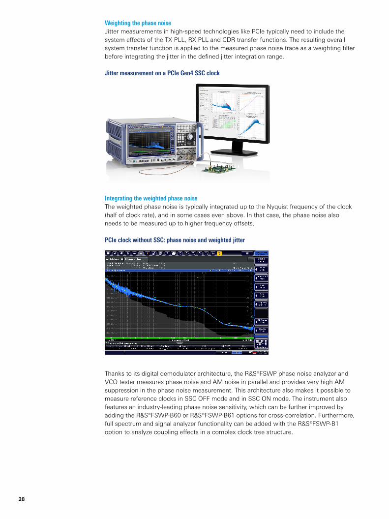
28

Weighting the phase noiseJitter measurements in high-speed technologies like PCIe typically need to include the system effects of the TX PLL, RX PLL and CDR transfer functions. The resulting overall system transfer function is applied to the measured phase noise trace as a weighting filter before integrating the jitter in the defined jitter integration range.

Jitter measurement on a PCIe Gen4 SSC clock

Integrating the weighted phase noiseThe weighted phase noise is typically integrated up to the Nyquist frequency of the clock (half of clock rate), and in some cases even above. In that case, the phase noise also needs to be measured up to higher frequency offsets.

PCIe clock without SSC: phase noise and weighted jitter

Thanks to its digital demodulator architecture, the R&S®FSWP phase noise analyzer and VCO tester measures phase noise and AM noise in parallel and provides very high AM suppression in the phase noise measurement. This architecture also makes it possible to measure reference clocks in SSC OFF mode and in SSC ON mode. The instrument also features an industry-leading phase noise sensitivity, which can be further improved by adding the R&S®FSWP-B60 or R&S®FSWP-B61 options for cross-correlation. Furthermore, full spectrum and signal analyzer functionality can be added with the R&S®FSWP-B1 option to analyze coupling effects in a complex clock tree structure.


PCIe clock with SSC: phase noise

In PCIe Gen4, a total of 64 different system transfer functions are defined for the 16 GT/s data rate. For each of these, the weighted jitter results need to be below the limit of 500 fs. For SSC clocks, the PCIe Gen 4 specification prescribes that the SSC spurs (funda-mental and harmonics) up to 2 MHz need to be removed before applying weighting and jitter integration. For easy handling, an external tool can be found in the download section of this application card. This tool automates the measurement and postprocessing of the data (SSC spur removal, weighting, jitter integration and identification of the highest jitter result out of the different system transfer functions). PCIe versions up to PCIe Gen 5 are supported.

PCIe clock with SSC: postprocessing of phase noise trace and PCIe jitter results

SummaryThe R&S®FSWP offers the functionality needed to test low-jitter clocks in both SSC OFF mode and SSC ON mode. It provides very high AM suppression in the phase noise measurement and excellent phase noise sensitivity for precise jitter measurements on low-jitter clocks for modern high-speed digital designs.

See alsowww.rohde-schwarz.com/product/fswp

30

VERIFYING THE CLOCK SOURCEThe signal purity of clock sources has a direct impact on system performance. To ensure proper operation, it is necessary to verify that the purity meets the design requirements.

YOUR TASKAs a designer of analog and digital circuits, you use and rely on the clock signal used in the target system. Since the clock directly influences overall system performance, it is essential that its performance be good enough to meet the needed requirements. In order to select or develop a clock generator to use in your design or to ensure that the supplied system clock has the proper performance once it reaches your section, you need to verify its performance to make sure it meets your needs. Phase noise, jitter, wideband noise and spurs are typical performance indicators.

ROHDE & SCHWARZ SOLUTIONThe R&S®FSWP phase noise analyzer and VCO tester is the right tool for verifying clock sources. Clock jitter is typically measured in the time domain. For superior sensitivity, users switch to the frequency domain to measure the clock jitter based on a phase noise measurement. The frequency domain approach also makes it easy to separate random jitter from periodic jitter, which can be easily determined by the spur level. Easily change-able integration ranges and weighting filters make it an even more powerful tool for jitter characterization with highest sensitivity.

Measuring the phase noise and jitter of the clock source with the R&S®FSWP

For measuring clocks with very low jitter, the R&S®FSWP can be equipped with a second internal local oscillator to allow cross-correlation and improve the phase noise sensitivity. To know how many correlations are useful, the instrument displays the achievable level of sensitivity with grey color-coding for a given setting. If the grey area is clearly below the trace, you know that the measurements are correct. Thanks to the extremely low-noise internal sources, only a small number of cross-correlations are needed to achieve a large sensitivity range. This speeds up measurement of clean signals dramatically.


The R&S®FSWP features ► Frequency range from 1 MHz to 8/26.5/50 GHz ► Up to 500 GHz with external mixers ► High sensitivity for phase noise measurements thanks to cross-correlation and extremely low-noise internal reference sources: typ. –172 dBc (1 Hz) at 1 GHz carrier frequency and 10 kHz offset, typ. –158 dBc (1 Hz) at 10 GHz carrier frequency and 10 kHz offset

A spectrum analyzer is typically used for spur searches. The R&S®FSWP includes a high-end spectrum and signal analyzer covering the full frequency range of the phase noise tester. You can search for spurs in the spectrum analyzer mode without any other instruments. Thanks to the large screen, you can configure multiple result windows in parallel on the display – and see the result of the phase noise measurements and the spectrum side by side.

The R&S®FSWP displays the achievable level of sensitivity with grey color-coding

The R&S®FSWP features

► Signal and spectrum analyzer and phase noise analyzer in a single box ► High-end signal and spectrum analyzer, 10 Hz to 8/26.5/50 GHz ► Wide dynamic range thanks to low displayed average noise level (DANL) of –156 dBm (1 Hz) (without noise cancellation) and high TOI of typ. 25 dBm

► 80 MHz signal analysis bandwidth ► Total measurement uncertainty: < 0.2 dB up to 3.6 GHz, < 0.3 dB up to 8 GHz

The R&S®FSWP includes a useful add-on as standard: low-noise internal DC sources for VCO characterization. It includes a power supply up to 16 V and a tuning voltage supply up to 28 V. Therefore, the power supply for the clock source module comes free. If the clock source is frequency tunable and based on a VCO design, tests over supply and tuning voltages are easily performed.

In short, the R&S®FSWP is the right tool for verifying the performance of the cleanest clock sources to ensure that the clock does not affect overall system performance.

32

Phase noise measurement and spur/harmonic search in the spectrum domain in parallel

See alsowww.rohde-schwarz.com/product/fswp

Application Notes ► A 1 MHz to 50 GHz Direct Down-Conversion Phase Noise Analyzer with Cross-Correlation

► Measurement Uncertainty Analysis and Traceability for Phase Noise


PRECISE MEASUREMENTS ON HIGH-SPEED DIGITAL SIGNAL LINES WITH THE R&S®ZNBWith continuously increasing data rates, signal inte grity aspects of high-speed digital designs and the components used become more and more challenging. Particularly at higher data rates, vector network analyzers (VNA) are increasingly replacing traditional time domain reflectometry (TDR) setups for testing passive components such as connectors, cables and PCBs. Users benefit from the higher accuracy, speed and ESD robustness of the VNA, making the VNA the instrument of choice in this field.

YOUR TASKWhen performing tasks such as verifying digital high-speed signal structures on PCBs, measurements have to be carried out on certain layers without the effects of probes, probe pads, vias, lead-ins and lead-outs. This requires the use of accurate deembedding algorithms to calculate and remove these effects from the measurements, leaving only the result for the area of interest.

ROHDE & SCHWARZ SOLUTIONThe setup below shows an example for verifying the high-speed differential signal lines on a PCB up to 20 GHz. The basis of the test setup is the R&S®ZNB20 four-port VNA. Corresponding deembedding tools (e.g. Delta-L, Delta-L+, PacketMicro Smart Fixture Deembedding (SFD) or AtaiTec In-Situ Deembedding (ISD)) can be run directly on the R&S®ZNB20, eliminating the need for an external PC.

R&S®ZNB20 setup to verify the high-speed differential signal lines on a PCB up to 20 GHz

34

Besides the actual signal trace to be measured, PCB test coupons typically also include a shorter signal trace to facilitate this deembedding. Differential PCB probes (e.g. from PacketMicro) are used to connect the R&S®ZNB20 to these signal traces.

Test setup

PROCESS AUTOMATIONTo streamline this procedure and guide the operator through the test steps, the test is typically automated via software. The screenshot below shows an example of the three steps of this test procedure:

► Measurement of a 2×thru (short) structure for deembedding, with results in the left column

► Measurement of the total (long) structure, with results in the center column ► Calculation of the area of interest based on the selected deembedding method, with results in the right column

The steps of the test procedure

For the 2×thru (short) as well as for the total (long) measurement, the impedance versus time of both probes is displayed above the insertion loss. This makes it easy to quickly identify whether a probe needs to be readjusted.

Reference planeafter calibration

Reference planeafter deembedding

Reference planeafter deembedding

Reference planeafter calibration

Area of interest


EYE DIAGRAMFor further investigations, the R&S®ZNB-K20 option can be used to analyze the eye diagram for the area of interest. This option also allows you to verify the effects of emphasis, noise, jitter and equalization in the eye diagram. It additionally provides a mask test with PASS/FAIL detection and statistic results.

Simultaneous display of eye diagrams and measurements in the frequency and time domain

SUMMARYR&S®ZNB offers all the functionality needed to test digital high-speed signal structures on PCBs in one box. Additional deembedding tools can be installed on the instrument to remove the effects of probes, probe pads, vias, lead-ins and lead-outs.

Ordering information

Designation Quantity Type Order No.Vector network analyzer

Vector network analyzer, 4 ports, 100 kHz to 20 GHz, PC 3.5 connectors

1 R&S®ZNB20 1311.6010.64

Time domain analysis 1 R&S®ZNB-K2 1316.0156.02

Extended time domain analysis 1 R&S®ZNB-K20 1326.8072.02

Calibration unit or calibration kit

Calibration unit, 10 MHz to 24 GHz, 4 ports, 3.5 mm (f)

1 R&S®ZV-Z52 1164.0521.30

Calibration kit, 50 Ω, 0 Hz to 24 GHz, 3.5 mm (m/f) 1 R&S®ZV-Z235 5011.6542.02

3683

.368

8.52

01.

00 P

DP

/PD

W 1

enR&S® is a registered trademark of Rohde & Schwarz GmbH & Co. KG

Trade names are trademarks of the owners

PD 3683.3688.52 | Version 01.00 | October 2021 (ch)

White paper | Know your jitter when debugging

Data without tolerance limits is not binding | Subject to change

© 2021 Rohde & Schwarz GmbH & Co. KG | 81671 Munich, Germany

Rohde & Schwarz customer supportwww.rohde-schwarz.com/support

Rohde & SchwarzThe Rohde & Schwarz technology group is among the trail-blazers when it comes to paving the way for a safer and connected world with its leading solutions in test & measure-ment, technology systems and networks & cybersecurity. Founded more than 85 years ago, the group is a reliable partner for industry and government customers around the globe. The independent company is headquartered in Munich, Germany and has an extensive sales and service network with locations in more than 70 countries. www.rohde-schwarz.com

3683368852

Documents

©Rohde & Schwarz; Know your jitter when debugging