1

Robust Scalability Analysis and SPM Case Studies*

Dejiang Jin and Sotirios G. Ziavras

Department of Electrical and Computer Engineering

New Jersey Institute of Technology

Newark, NJ 07102

Author for Correspondence

Professor Sotirios G. Ziavras

Department of Electrical and Computer Engineering

New Jersey Institute of Technology

Newark, NJ 07102

ziavras@adm.njit.edu

Telephone: (973) 596-5651

Fax: (973) 596-5680

* This work was supported in part by the U.S. Department of Energy under grant DE-FG02-03CH11171 and the National Science Foundation under grant CNS-0435250.

2

Abstract

Scalability has become an attribute of paramount importance for computer systems used in

business, scientific and engineering applications. Although scalability has been widely discussed,

especially for pure parallel computer systems, it conveniently focuses on improving performance

when increasing the number of computing processors. In fact, the term “scalable” is so much

abused that it has become a marketing tool for computer vendors independent of the system’s

technical qualifications. Since the primary objective of scalability analysis is to determine how well

a system can work on larger problems with an increase in its size, we introduce here a generic

definition of scalability. For illustrative purposes only, we apply this definition to PC clusters, a

rather difficult subject due to their long communication latencies. Since scalability does not solely

depend on the system architecture but also on the application programs and their actual

management by the run-time environment, for the sake of illustration we evaluate scalability for

programs developed under the super-programming model (SPM) [15-17].

Keywords: scalability analysis, distributed processing, parallel processing, heterogeneous cluster

3

1 Introduction

Generally scalability relates to the possibility to build larger systems to address larger problems

without significant performance degradation due to increased communication and other latencies in

the parallel or distributed environment. Scalability has become a critical attribute of computer

systems and/or software solutions in various application domains for economical and technical

reasons. Different users may have different expectations from computer systems, such as their

computing capacity. The particular user’s requirements may also be subject to change with time.

For example, a business user may initially need a small computer system to satisfy basic

requirements and then may demand a more powerful system for larger business tasks. Actually

many servers increase their user base daily and their application datasets become ever larger. In

practice, it is neither possible to design and build a computer system for each user, nor to replace

computer systems very often. Therefore, the solution to address demand diversity is to make

systems adaptable and scalable. That is, keeping the basic features of computer systems, more

resources could be added easily to satisfy higher demands. This way a computer system could

satisfy many users or applications for relatively long periods of time.

The primary objective of scalability analysis is to characterize computer systems in a way

that can convince users that they can still work well with larger workloads. Intuitively, scalability is

an attribute of a scheme, design, architecture or solution for a device or system as it pertains to

solving large problems. When users have an overall solution (e.g., a pair of a computer system and

an algorithm) to solve a particular problem or provide particular service for a certain problem size,

they usually want to know 1) how well the solution works for larger problems (i.e., if the results are

produced quickly enough or an acceptable service level is possible). If the predicted results cannot

achieve the desired goal (in execution time or service quality), they may also want to know 2) if

they can keep the software solution but increase the system resources to reach another desired

performance level. In the latter case, they may even want to know 3) how many resources must be

added to achieve this goal and what extra cost is required. To answer these questions, scalability

studies should incorporate robust quantitative metrics to analyze their solution. If the answer to

question 2 is affirmative, the solution can still be called “scalable.” When comparing different

solutions that solve the same enlarged problem at comparable performance levels, the solution that

requires fewer resources has better scalability.

4

In general, scalability measures the capability of a solution to maintain or increase the

performance when the problem and/or computer size increases. For this reason, relationships

between the performance and the problem size, and/or the computer size are often quantified [6, 11-

13]. Researchers have used various performance metrics and techniques in their definition of

scalability which is expressed in the form of a single index [3-5, 8, 9]. Most often, scalability is

associated with parallel computer systems. A study of the parallel performance of aerodynamic

simulation packages on the NASA Columbia supercomputer was presented in [20]. Results demonstrate

good scalability on up to 2016 CPUs using the NUMAlink4 interconnect and indicate that larger test cases on

larger systems implementing combined MPI/ OpenMP communication should scale gracefully. [21] claims

that the parallel computation of numerical solutions to elastohydrodynamic lubrication problems is

only possible on fine meshes by combining multigrid and multilevel techniques. A performance

model for such a solver was developed to analyze scalability. The authors of [22] claim that the

number of processors in high-end systems is expected to rise by the end of this decade to tens of

thousands (e.g., IBM BlueGene/L). Therefore, known scalability and fault-tolerance deficiencies of

scientific applications must be investigated. A 100,000-processor simulator is discussed. [23]

presents a parallel algorithm for 3D FFT on a 4096-node QCDOC, a massively parallel

supercomputer with tens of thousands of nodes residing on a 6D torus network. To produce graceful

performance, simultaneous multi-dimensional communication and communication-and-computation

overlapping were employed. Benchmarking demonstrated good performance improvement for up to

4096 nodes. The results also suggest that QCDOC is more scalable than the IBM BlueGene/L

supercomputer for 3D FFT.

None of the current scalability models/definitions are appropriate for all computer

architectures because of their narrow focus on a few parameters and their limited search space. To

make possible a study of scalability for various types of computer systems and algorithms, we

introduce a generic definition. We strongly believe that scalability ought to be a comprehensive

attribute than can be hardly expressed by a single index. Therefore, we employ a directional

derivative of a performance metric to quantify scalability. Since researchers can expand all the

design dimensions of interest and collapse all the other dimensions, this kind of scalability

definition facilitates an analysis to find an optimal path to scale up a system for a given problem

solution; it also supports a comparison of potential solutions. For each scenario of scaling up a

system, researchers may need to collect performance data from experiments or employ a

performance metric model.

5

In Section 2, we discuss the need for a robust definition of scalability and present current

definitions along with their limitations. In Section 3, we present a new quantitative definition of

scalability with wide focus and set up a methodology to carry out scalability analysis based on the

new definition. Section 4 tests the robustness of our scalability definition and our analysis

approach; techniques to scale up PC clusters are discussed and the scalability properties of

programs developed under our SPM model are also presented. We point out a way to effectively

scale up PC clusters under SPM to support calculations for very large problems. Our robust

definition of scalability for parallel programs further clarifies issues related to the behavior of

parallel programs on PC clusters, an often complicated topic for users. For illustrative purposes

only (to show how our scalability analysis approach can be applied), case studies of scalability for

PC clusters are presented in Section 5. Experiments on hierarchical PC clusters and relevant

scalability analysis results are presented in Section 6.

2 Scalability Issues and Current Approaches

2.1 Scalability as a Comprehensive Entity

As mentioned earlier, scalability is primarily a qualitative attribute of an algorithmic solution to a

given problem in association with a computer system. Neither the properties of the architecture nor

the properties of the algorithm can be used exclusively to determine scalability [1, 4-10, 20-23].

Solutions adopting the same application algorithm may have different scalabilities. It is possible

that the implementation of the algorithm on one system is scalable but another implementation of

the same algorithm on another system with different architecture is not scalable. Claiming that an

algorithm is scalable may only mean that there is an architecture on which the solution of this

algorithm is scalable. In theory, the architecture may be an ideal computer model, such as the

PRAM. Similarly, we cannot consider only a computer system or architecture without mentioning

an algorithm or a problem. Sometimes the system can be expanded rather easily to potentially

accommodate larger problems. There is a working window where the implementation of some

algorithms on an expandable architecture often improves performance [18, 19]. This is also true for

PC clusters.

From the point of view of quantitative analysis, scalability depends on many factors that

characterize both the architecture and the algorithm. For example, to determine the scalability of

matrix multiplication, one may need to know the size of the matrices, their type and their sparsity;

6

for a distributed multi-computer system, one may need to know the number of processors, the size

of the memories attached to the processors, and the number and type of communication channels

interconnecting these processors along with their bandwidth. Current practices in scalability

analysis do not provide a direct way to take into account large numbers of parameters reflecting the

detailed features of the application algorithm and the target computer system.

2.2 Existing Scalability Definitions

The various definitions of scalability come from similar motivations [10]. A widely used definition

employs the asymptotic speedup metric S(p, n), where p is the number of processors and n is the

problem size [5]. Speedup is defined as the ratio of the serial run time Ts(n) of the best algorithm

that solves the given problem of size n to the time T(p, n) taken by the selected parallel algorithm

for the same problem with p processors. Formally,

S(p, n) = Ts(n) / T(p, n) (1)

for a problem of fixed size. However, this definition may ignore significant non-primary terms

related to overheads; this asymptotic behavior study may not be practical in real program runs. The

definition should actually use the exact order Θ notation.

The simplest definition of scalability uses the system efficiency [2] which is given by

Sc = S(p, n) /p (2)

The authors then introduce the iso-efficiency concept for an algorithm–system pair; it states that the

efficiency should be fixed in scalable problem-system pairs independent of their sizes. For a fixed

Sc > 0, we can then approximate the execution time when the system size increases:

T(p, n) = Ts(n)/ (Sc * p ) (3)

Since all overheads are reflected in the parallel execution time T(p, n), we could find how many

processors to add to the system to decrease the execution time to a desirable level:

p = Ts(n)/ (Sc * T(p, n) ) (4)

This definition has the disadvantage that users are not normally expected to know in advance the

best efficiency for a given pair.

7

Another definition of scalability for a given architecture-algorithm pair uses the ratio of the

asymptotic speedup of the algorithm on this architecture to its asymptotic speedup SI(p, n) on an

ideal machine (such as the PRAM) with the same number of processors [5]:

Sc = S(p, n) / SI(p, n) (5)

This definition finds the effect of the architecture choice by comparing with the best possible

performance on an “ideal” machine. This approach is not practical for a given system that has to be

modified appropriately to get better performance. [1, 13] focus exclusively on problems that are

inherently scalable primarily because of data parallelism. Such problems appear in scientific

applications (such as weather modeling) where the size of the input data set can be increased

“indefinitely” to produce higher accuracy in the solution. Business and many other applications,

however, do not often follow this pattern or sometimes users are interested in finding out how

performance improves with limited resource improvements that focus on specific aspects of the

computer system.

2.3 More on the Limitations of Current Approaches

Scalability analysis relies on a chosen theoretical methodology to analyze performance for various

problem and system sizes. However, current methods of scalability analysis have major limitations

as there are inadequacies in their definition of scalability as well as the analysis approaches taken by

them. A major disadvantage comes from adopting asymptotic terms in the definition of scalability.

Two problems show up. The first one is practical since users are forced to care about performance

when the system size varies in a tremendous range. However, most architectures work well for

given problems only when the system size changes are of limited scope. Asymptotic scalability

analysis may miss too much important information in practical cases. Performance behavior due to

changes in the system size within a specific practical range may be very different from that of

asymptotic changes. The second problem stems from the fact that the performance of very large

systems normally deteriorates rapidly due to intolerable latencies.

The second disadvantage is that these definitions measure the system size based exclusively

on the number of processors. They assume that the performance of programs depends primarily on

the number of processors and less on other resources in the system. Under this assumption, several

scalability analyses only account for the overhead of communication [7]. However, this is not

sufficient. As discussed earlier, the performance depends on both the problem and system sizes.

8

Actually representing the system “size” may require multiple parameters rather than just the number

of processors. Besides processors, a system may be increased in size by installing several additional

resources (e.g., memory) to improve its performance. Increasing the amount of available memory

can improve the scalability of memory-bound problems such as the sorting of very large data sets.

Ignoring these other types of resources may have an adverse effect on performance estimation.

Although scalability analysis exclusively for memory-bound problems has been pursued before, an

integrated approach that incorporates many choices for system changes has not been attempted. In

general, these approaches are incomplete.

To make scalability analysis practical, one usually builds an execution model depending on

some assumptions. A widely accepted implicit assumption is that the execution time of all the basic

processor operations is constant and does not depend on the overall system size. Based on this

assumption, the sequential execution time of a program can be estimated by its total number of

basic operations. It is often called the workload Wideal(n) of the problem. The cost of solving a

problem on a p-processor system can be defined as p * Tp(n); it is the maximum number of

operations in the parallel execution time Tp(n) and is expressed in time units for basic operations.

During execution, the p processors perform useful operations to solve the problem and operations

resulting in overhead. If Woverhead(p, n) represents all the operations corresponding to overhead,

including the idle time of processors, then:

p* Tp(n) = (Wideal(n) + Woverhead(p, n)) * t0 (6)

where t0 is the execution time of a basic operation. If Woverhead(p, n) can be estimated, then the

execution time Tp(n) can be approximated and the system size can be derived to solve a problem of

given size in a specified amount of time. Most scalability analyses focus on the overhead function

Woverhead(p, n), only estimating the amount of additional operations due to communications. A

drawback is that this estimation does not count idle times. Also, it is difficult to estimate this

function when the system size changes in a wide range and/or non-processor resources increase as

well.

3 Robust Scalability Analysis

3.1 Robust Definition of Scalability

An application problem is characterized by two sets of attributes. One relates to the methodology

(i.e., the chosen algorithm). The other is a set of parameters that relates to the characteristics of the

9

input (such as the dimensionality and sparsity of matrices in matrix multiplication). The latter

parameters (p1, p2, …, pj, …) are simply collectively referred to as the size of the problem; they can

be denoted with a vector P(p1, p2, …, pj, …) in the problem space P. Each point in this space

represents a particular size for the problem.

A computer system also can be described with two sets of attributes. The first set of

qualitative attributes identifies the system’s specific architecture. For example, a PC cluster consists

of a set of autonomous PCs which are connected to each other via a standard local network. The

type/class of nodes and the type of network should be included in this set. The other is a set of

quantitative attributes Q which specify the system’s detailed characteristics. For example, a PC

cluster can be characterized by its number of nodes, the total amount of memory per node and the

bandwidth of the network. Each member value quantifies the system in a specific aspect. The

specific system condition can be identified with a vector R(r1, r2, …, ri, …) in the multi-dimensional

system space R. Among the set of quantitative attributes there is a subset associated actually with

the system’s size (e.g., number of nodes). Therefore, the size of the system can be projected as a

vector R(r1, r2, …, ri, …) into a sub-space of R. Each point in this space represents a particular

instance of the computer architecture which can be quantified.

Using the cross-product space N of R and P (or, equivalently, the cross-product space M of

Q and P) for our values domain, we can study scalability. The vector N(r1, r2, …, ri, …; p1, p2, …,

pj, …) in space N denotes an implementation case of running the program of specific size on the

specified system with specific quantitative attributes. For each such implementation case, there is

an associated performance metric

U= U(R, P) (7)

This function should completely profile the performance of the algorithm on the given instance of

the computer architecture. The metric U could be defined as any quantitative index that can

measure the degree of user satisfaction. For example, the chosen metric could be throughput for

service programs. For most computational programs, the metric could be the execution “speed”

defined as 1/T, where T = T(R, P) is the execution time of the program.

The scalability Sc at a particular point (R, P) can now be defined as the directional

derivative of the considered metric along a particular dimension in the new space N. That is:

10

Sc (V, R, P) = (U(N+ΔN)-U(N))/δ (8)

where δ is a small scalar, ΔN = δ V and V is the unit vector in the specified dimension. While the

system resources R increase, the problem size P is fixed or increases simultaneously in space N. Of

course, N represents the pair (R, P).

When Sc(V, R, P) > 0, we can say that the system-problem pair (R, P) is locally scalable in

direction +�N of the chosen dimension. Based on this definition of scalability, it is easy to

conclude that the result does not depend on the selection of any reference case. The term locally

scalable targets improvements at a given design point (i.e., with known values for the design

parameters). On the other hand, the term globally scalable is used to denote scalability analysis

comprising the wider multidimensional space.

3.2 Direction of Preferred Scalability

This definition of scalability is generic for a single dimension. Besides the chosen computer

architecture and algorithm pair, the scalability also depends on the way chosen to increase the

system size and/or problem size; i.e., scalability must be studied in reference to dimensions and

directions of change. Different analysts may have different considerations and may get different

conclusions regarding the scalability of a solution. Scalability analysis in all directions is needed to

completely characterize a solution. Scalability analysis in a particular dimension will give a

solution under a set of specific constraints. Under some constraints, scalability analysis may be

reduced to existing analyses discussed earlier. By selecting 1/T as the metric of user satisfaction

and normalizing to a reference case that solves the problem on an optimized sequential computer,

we get

U= (1/Tp(R,P)) / (1/Ts(P)) = Ts(P)/Tp(R,P) (9)

which is simply the speedup; Ts(P) and Tp(R,P) represent the sequential and parallel execution

time, respectively. Under the constraint that the system is increased in size by simply adding more

processors (a practical example is a multiprocessor computer with centrally shared memory) while

the problem size stays fixed, the obtained scalability corresponds to the first definition. Similarly, if

the problem size increases linearly with the number of processors and all other system parameters

are kept constant, we study scalability according to the definition of scaled speedup [1].

11

Since PC cluster systems are normally increased in size by adding more member computers,

the numbers of many and diverse system resources (including processors, memory, NICs, etc.)

increase as well. Therefore, it is more reasonable to analyze scalability along the direction in which

the relevant parameters of the associated resources increase simultaneously and linearly.

3.3 Cost Study for Optimal System Expansion

As mentioned above, the primary purpose of scalability analysis is to ultimately help users decide if

a system can be scaled up graciously to solve a larger problem. Quantitative analysis can help

decide how exactly to scale up a system to improve a measure, such as performance. However,

users usually have a comprehensive cost metric for system updates as well. Some updates may be

scalable but their cost may be prohibitively high. The cost of an update can be represented by

cost = VP * VU = Σi (Pricei * Δri ) (10)

where VP = (Price1 , Price2 , …, Pricei , …) is a vector of prices for the considered resources and

VU = ΔR = (Δr1 , Δr2 , …, Δri , …) is a vector of resource changes (in arbitrary units); Δri = (ri

− rio) ≥ 0. We can assume for the sake of simplicity that, if ri expresses the resource amount in

linear scale, then Pricei gives the regular price of the i-th type of resource; if ri expresses the

resource amount in logarithmic scale, then Pricei gives the price when doubling the i-th type of

resource. An optimization problem is to update various types of resources for maximum scalability

benefits under a given total cost increase. The users may conveniently define the efficiency of

updates for system-problem pairs as

E = ΔU/cost = (U(N o +ΔN)-U(N o))/ Σi (Pricei * Δri)

= (U(R o +ΔR, P o +ΔP)-U(R o, P o))/ Σi (Pricei * Δri) (11)

where Ro{r1o

, r2o

, …, rio

, …} is a reference system configuration, Po{p1o

, p2o

, …, pjo

, …} is a reference

problem size, R{r1, r2, …, ri, } is the scaled up system and P{p1, p2, …, pj, …} is the problem under

study. In this case, the optimality problem is to find the direction in which the efficiency of the

update is maximized; i.e., find the direction corresponding to the largest possible value of ΔU for a

given maximum update cost.

Based on field theory, in a range enclosing a reference system configuration Ro the increase

in U achieved by moving the system state from Ro to R along vector VU will be

12

ΔU = grad (U) * VU (12)

where grad (U) is the gradient of U [14]. Thus, the scalability in the i-th dimension is

Sci, ΔP = (U(R o +Δri, P o +ΔP)-U(R o, P o)) / Δri . (13)

Based on equation (11), the efficiency of the system update is

E = [grad (U) * VU] / [VP * VU] (14)

We can prove that if (Sck, ΔP/ Pricek) > (Sci, ΔP/ Pricei) for all i ≠ k, then increasing the resources in

the k-th dimension yields the most efficient solution. We can also prove that if there are two or

more dimensions that maximize Sci, ΔP/ Pricei, then a combination of resource updates in a subspace

could yield the same efficiency. The proof is included in the Appendix.

4 Scalability Analysis for PC Clusters Under SPM

Scaling up a system is the basis for users to improve performance in order to solve a larger problem

and/or solve the same problem more quickly. Scalability analysis provides a tool to find the most

effective and economic ways to scale up systems. For each possible solution, researchers may need

to collect performance data from experiments or employ a performance metric model. Scalability

analysis for PC clusters is undoubtedly of paramount importance as the majority of high-

performance systems are of this type. In this section we apply our scalability method to examples

that illustrate how to use our analytical approach. Since our main purpose in these examples is to

find efficient ways to organize PC clusters, we are less interested in the internal architecture of

individual PCs; therefore, we collapse most of the dimensions that characterize the properties of

individual PCs.

4.1 Techniques for Scaling Up PC Clusters

PC clusters can be scaled up in many ways that can be roughly classified into two categories. One is

increasing the number of computer nodes in the cluster. The other is scaling up the member nodes

by improving their capabilities. The first technique is straightforward and essential in scaling up PC

clusters, as long as the new nodes can work seamlessly in the system. This way various types of

resources in a PC cluster can be increased simultaneously. Besides increasing the number of

processors, the total memory in the cluster also increases. The number of nodes in the cluster may

13

still be a good parameter to denote system size. However, newly installed PCs do not have to be

identical to previous PCs. They may have more processors, more memory, may be equipped with

more powerful processors or faster memory, etc. This approach may result in a heterogeneous

cluster. Then, the number of nodes may not be a good parameter to denote system size.

The second category of techniques scales up a PC cluster by increasing the number of

resources in member nodes or improving their capabilities. These techniques may be applied in

many different directions. One may increase the number of processors in individual nodes, the

memory in the nodes individually or simultaneously, etc. Such approaches can improve a PC

cluster to help end users solve larger problems in the requested time. The idea of scaling up clusters

by modifying member nodes can have a wider meaning. People may treat each member computer

in the PC cluster as a logic subsystem. They can then scale up subsystems by replacing member

computers with entire PC clusters. This way, a PC cluster will become a hierarchical structure of

many levels providing many opportunities.

Denoting the size of a hierarchical PC cluster via multiple parameters is reasonable and

makes robust scalability analysis tractable. For the sake of simplicity, we assume homogeneity in

the following examples (i.e., the PCs are identical). In the real world, newly added PCs may be

more powerful than older ones. We can then assume heterogeneity at the lower level but view the

logic nodes at the next level as almost identical; i.e., the new logic nodes at the higher level will

have almost identical computation complexity but will consist of fewer member PCs. The size of a

homogeneous PC cluster with a k-level hierarchical structure may be denoted with the data set R{r1,

r2, …, rj, …, rk, rc, rm}; r1 is a parameter for the number n1 of nodes at the topmost (first) level, r2 is a

parameter for the number n2 of nodes in a subcluster that serves as a node in the first level structure;

similarly, rj (for 1 < j ≤ k) is a parameter for the number nj of nodes in a subcluster that serves as a

node in the (j-1)-th level structure. We select a logarithmic expression for these parameters, i.e., rj =

log nj. For a k-level system, each k-th level subcluster consists of an atomic PC; rc is a parameter

for the number of processors in the PC and rm is a parameter for the memory size in each PC. There

may be more parameters needed to characterize the size of last-level atomic computers; we ignore

them here for the sake of simplicity.

This hierarchical approach provides significant flexibility in building PC clusters, thus

improving their scalability features. For example, assuming a uniform cluster with four levels and

14

32 nodes per subsystem (i.e., r1 = r2 = r3 = r4 = 5) the resulting system is huge consisting of about

one million or 220 PCs.

4.2 Scaling Up Programs Developed Under SPM

Scaling up a PC cluster is just an instrument to help users solve larger problems. However, they

should care about the performance of their software solution on the scaled up system as well. The

factors that affect the scalability of a program under a given programming model constitute two

groups. One group is related to the scalability of the program on the given architecture; the other is

related to the scalability of the implementation in terms of basic operations. The following example

illustrates the difference between these two groups. Assume the problem of multiplying two dense

matrices of size M × M on p “processors.” If these processors can collectively perform

multiplication and addition of two dense matrices of size m2 × m2 directly (i.e., in constant time),

where m2 ≤ M, then the computation complexity of the program is W(m1) ≈ const* (m1)3, where m1

= M/m2. Considering the overhead in terms of additional basic operations Wo(p, m1), the execution

time of the program running on this computer system will be

T(p, f, m1, m2) = C(p, m1) * t(f, m2) = {[W(m1)+Wo(p, m1)] /p} * t(f, m2) (15)

where f is a performance metric of the processors (e.g., the MIPS rate) and t(f, m2) is the average

time to perform a basic operation on these processors. When users need to multiply larger matrices

(i.e., with larger M) but keep the total execution time at the same level, they can either increase the

number p of processors to decrease the first factor C(p, m1) or increase the computation

performance f of the processors to decrease t(f, m2). The effect of these techniques depends on the

real values of m1, m2, f and p. C(p, m1) characterizes the scalability of the program itself while t(f,

m2), on the other hand, characterizes the scalability of basic computer operations.

Few of the existing programming models mention the effect of implementing basic

operations on the overall scalability of the solution. The primary reason is that most of these

programming models do not provide a mechanism to scale up the set of supported basic operations.

They use directly the instruction set of the processor to derive their basic operations. However, the

problem size that can be solved directly with the instruction set of a processor is usually fixed. For

example, COTS (commercial off-the-shelf) processors for PCs often support only the multiplication

of a pair of scalar variables (i.e., in terms of dimensions they only implement directly the

15

multiplication of matrices of size 1 × 1). Besides this, processors are normally impossible to scale

up since their resources cannot be increased after they have been manufactured.

Our super-programming model (SPM), however, can fully exploit the scalability in basic

operations [15-17]. This is because the basic operations under SPM are coarse-level super-

instructions. SPM integrates both message passing and shared memory. Under SPM an effective

instruction-set architecture (ISA) is to be developed for each application domain [15]. Frequently

used operations in that domain should belong to this ISA. The Super-Instructions (SIs) in the ISA

are to be developed efficiently in the form of program functions for individual PCs in the cluster.

The operand sizes (i.e., function parameter sizes) for SIs are limited by predefined thresholds.

Application programs are modeled as Super-Programs (SPs) coded with SIs. Under SPM the

parallel system is modeled as a virtual machine (VM) which is composed of a single super-

processor that includes an SI fetch/dispatch unit (IDU) and multiple SI execution units (IEUs). For

PC clusters, an IEU is a process running on a member node that provides a context to execute SIs.

SIs are dynamically assigned to IEUs based on a producer-consumer protocol. The IDU assigns

SIs, from a list of SIs ready to execute, to IEUs as soon as the latter become available. The super-

processor can handle a set of “build-in” data types that form operands for SIs; they are called Super-

Data Blocks (SDBs). All application data are stored in SDBs which can be accessed via appropriate

interfaces. The runtime support system provides local data representation for SDBs. Each SDB can

be incarnated into a set of objects distributed throughout the cluster. The SPM runtime support

system controls the incarnated objects during their lifecycle based on their usage [16]. Thus, the

logic of scheduling and distributing tasks can be decoupled from the actual data distribution and the

impact of the latter on workload balancing is reduced dramatically. The aforementioned set of

incarnated objects represents a coherent data entity. They cooperate with each other with the

mediation of the runtime system. Such multiple distributed representations can serve efficiently the

demand for data by multiple SIs. Our approach increases the number of SIs executing in parallel by

minimizing thread stalling. The reader is encouraged to read [15, 16] for more details.

The size of the problem solved by an SI depends heavily on its SDB operands that have

configurable size. Also, SIs execute on the IEU virtual functional unit which can be implemented

with scalable hardware/software systems such as symmetric multiprocessors or even PC clusters. In

this situation, exploiting the scalability of basic operations may make the programs more scalable.

Let us review the previous example of matrix multiplication. When the size M of the input matrices

16

doubles while m2 is kept fixed, the complexity W(m1) of the program will increase eight times and

the overhead Wo(p,m1) may increase more. In this case, increasing the resource processors by a

factor of eight cannot keep the total execution time unchanged. In our pilot experiments for sparse

matrix multiplication, the overhead typically increases by more than x=20%. However, keeping m1

(i.e., the number of blocks the matrix is divided into) and the number of IEUs fixed will not

necessarily change the complexity of the super-program and the overhead. This increase in the

problem size can be handled without a time penalty at this level by increasing the problem size for a

basic operation (i.e., m2) and scaling up the system by increasing the resources in each IEU by a

factor of eight. If t(f, m2) increases by less than x when m2 doubles and the individual node

performance f increases eight times, this approach will be better than the previous one. This

example shows that scaling up the SI provides a powerful instrument to improve the overall

scalability.

In this example we pay less attention to the capabilities of the communications

infrastructure. The characteristics of the channels running between different levels in the hierarchy

do not resemble those inside an individual level. The sensitivity of the performance to the

communication latencies depends heavily on the chosen programming model. For example, SPM

implies larger task granularity and larger amounts of data transfers at higher levels. This approach

results in very substantial overlaps of communications with computations at lower levels.

Therefore, the hierarchical cluster can be assumed to be uniform between levels even though

communications between PCs that belong to different subclusters are much slower than those

between PCs inside the same subcluster.

4.3 Scalability of Super-Programs on Hierarchical PC Clusters

SPM matches very well the architecture of PC clusters with multi-level structure. SIs are

implemented with procedures executing on member nodes in the cluster. When a member node

itself is comprised of another lower-level cluster, these SIs can still be implemented under SPM;

i.e., they are similar to super-functions (SFs) that can be coded with lower-level SIs. Such a

hierarchical structure can be extended until the lowest level is an atomic PC, as discussed earlier.

Finding the optimal parameters for SIs at various levels of the hierarchical cluster involves

multiple solution subspaces. Each subspace involves problem and resource sizes; for the sake of

17

simplicity, we assume here a homogeneous cluster where the latter is simply the number of member

nodes. Based on our earlier discussion, the total execution time is

T(r1, r2, …, rk, p1, p2, …, pk, pk+1) = ( ∏i Ci(ri, pi )) * t(pk+1) (16)

where ri is the parameter for the resource size of the i-th level cluster, p1 is the problem size in terms

of operands for first-level SIs, C1(r1, p1) is the complexity of the problem including all associated

overheads in number of first-level SIs, pi (for i = 2, …, k) is the problem size for SIs in (i-1)-th

level clusters, Ci(ri, pi) (for i = 2, …, k) is the average complexity including all associated overheads

of (i-1)-th level SIs in number of i-th level SIs, pk+1 is the problem size for k-th level SIs and t(pk+1)

is the average execution time of k-th level SIs on atomic PCs. ri may be expressed as log2ni, where

ni is the number of member nodes in an i-th level cluster. The total number of atomic PCs in the

cluster is n = 2r, where r = r1 + r2 + … + rk. The overall problem size in number of basic

instructions for atomic PCs is p = p1 * p2 * … pk * pk+1. Increasing the total number of atomic PCs

m times can be achieved by increasing the number of nodes m times at any level. Similarly,

increasing the problem size pi at the i-th level q times also increases the overall problem size q

times. If we adopt U(R, P) = log(1/T(R, P)) as the performance metric (all logarithms here have the

base 2) and r=log n as the resource metric, then according to Equation 13 the scalability of (i-1)-th

level SIs is represented by

Sci, ΔP = log (Ci(rio

, pio) /Ci(ri, pi )) / Δri (17)

It only depends on the algorithm adopted for the i-th level.

From the results in Section 3 we know that the dimension with the maximum value for

Sci,ΔP/ Pricei is the most efficient to update (see Equation 14). This will be referred to as the edge-

scalability of the solution.

4.4 Scalability of an Optimally Configured Solution for a PC Cluster

Now let us discuss some important properties of scalability for a well configured solution. For the

sake of simplicity, we assume that the overall problem size is constant and the performance metric

is the logarithm of the speedup. For Δri = 1, which means that log ni – log nio = 1, we have ni = 2 *

nio and

Sci, ΔP = log (Ci(rio

, pio) /Ci(1+ri

o, pi ) ) (18)

18

Therefore, the scalability can be expressed with logarithmic execution time decreases when the

resources double.

A multi-level PC cluster can be easily reconfigured and the programs developed under SPM

can also fit the reconfigured system by adjusting the parameters for SIs. The basic reason is that

scaling up levels requires the same “raw material”—PCs. An optimal configuration provides

maximum performance under a given amount of resources. The first property of an optimally

configured cluster is that the scalabilities of all its non-leaf levels are identical. The fundamental

reason is liquidity of resources. Reconfiguring the system then simply requires reducing the

resources in one level to scale up another level. This is proved as follows. If Sci, ΔP < Scj, ΔP (for i, j

< k), we can always reduce the number of nodes in each j-th level cluster while increasing the

number of nodes in each i-th level cluster. For this adjustment

ΔU = U(R o +ΔR, P o +ΔP)-U(R o, P o) = Sci, ΔP * Δri + Scj, ΔP * Δrj (19)

where Δri = - Δrj > 0; therefore, ΔU = (Sci, ΔP - Scj, ΔP) * Δri > 0. It means that the current

configuration is not optimal if the scalabilities of non-leaf levels are not the same. The resources at

the lowest level are not interchangeable with resources at other levels since leaf nodes are atomic

PCs. Normally we can neither take apart single PCs to build two or more PCs nor merge the

resources of multiple PCs into a more powerful PC. However, since a PC usually has many

resources, the problem size for SIs executing on a PC can vary in a wide range. Users can

reconfigure the task grains between atomic PCs and upper level clusters to pursue maximum

performance. Therefore, the PC level should have the same scalability with other levels; it can be

obtained by appropriate task assignment. This means that a well configured PC cluster should have

the same scalability at all the levels; it should be close to the edge-scalability (as defined earlier).

Another property of an optimally configured cluster is that its edge-scalability should not be

less than the scalability Sc0 of the initial cluster when a PC is replaced with a two-node cluster; that

is,

log (Ci(rio

, pio)/ Ci(1+ri

o, pi) ) ≥ Sc0 (20)

where Sc0 = log Sp0 and Sp0 is the speedup of a two-node cluster.

19

Equation 20 should hold for all rio

= 0, 1, 2, …, ri-1, if Sci is to decrease monotonically.

Then, log Ci(0, pi) Ci(ri, pi) = log [

Ci(0, pi) Ci(1, pi)

Ci(1, pi) Ci(2, pi) …

Ci(ri -1, pi) Ci(ri, pi) ] and, therefore, log (Ci(0, pi)/ Ci(ri,

pi)) ≥ ri *Sc0. Then, based on Equation 15 the overall speedup of the solution is

Speedup = T(0, 0, …, 0, p1, p2, …, pk, pk+1)/ T(r1, r2, …, rk, p1, p2, …, pk, pk+1)

= ∏i (Ci(0, pi )/Ci(ri, pi )) ≥ exp{ (∑i ri)*Sc0 } = (Sp0 )r (21)

where r = ∑i ri = log n, n is the total number of PCs and Sp0 is the average speedup of a two-node

cluster for the SIs. The efficiency of the solution is then

E = Speedup / n ≥ (Sp0 / 2) r (22)

or

log E ≥ (Sc0 – 1) * log n (23)

5 Case Studies

To showcase our proposed scalability analysis approach, let us take a look at a few cases of matrix

multiplication. That is, the purpose of this section is to show only how our scalability analysis

approach can be applied. We assume a two-level cluster system represented with the pair of

parameters (r1, r2) that denote size, as previously. Also, the input matrices are assumed partitioned

into primary submatrices (i.e., level-1 SDBs) which are partitioned further into basic (i.e., level-2)

SDBs. Multiplying a pair of matrices is implemented with primary or level-1 SIs. Each primary SI

performs multiplications/additions for a pair of level-1 SDBs on a level-1 node in the cluster; these

SDBs are produced by the multiplication of submatrices of size m2 × m2 at level 2. A level-1 node

is itself a cluster (i.e., a level-2 cluster) that consists of many atomic PCs. Each primary SI is

implemented with level-2 SIs. Multiplying a single pair of level-2 SDBs can be performed by a

single level-2 SI on an atomic PC. We assume that the size of these SDBs is constant and the

workload of each level-2 SI is constant. Also, the average execution time of level-2 SIs is T2.

The primary super-program and the SIs at both levels can be developed under SPM.

Therefore, the SI execution times can be estimated. Assume that the workload of a primary SI is

expressed in number w2 of level-2 SIs. The average execution time of a primary SI is then

T1 = C2(r2, m2) * T2 = {[w2+Wo2 (n2,w2) ] / n2 } * T2 (24)

20

where Wo2 represents the overhead for level-2 execution. The total execution time of the super-

program for matrix multiplication is

T = C1(r1, m1) * T1 = {[w1+Wo1 (n1,w1) ] / n1 } * T1 (25)

where w1 is the workload of the program expressed in number of primary (level-1) SIs and Wo1 is

the overhead at this level. Under SPM, the most important overhead is due to workload imbalance

since the primary objective is to minimize the idle time of cluster nodes through multithreading

[15]. This overhead can be expressed simply as

Woi = ci* (ni -1), for i = 1, 2 (26)

where ci = bi - ai. bi is the maximum number of SIs assigned simultaneously by IDU to a node to

execute with multithreading; ai is the average number of SIs per node that are executing on the other

ni -1 nodes when the last set of SIs in the super-program are assigned to a node. ci* Ti is the

expected average idle time of the other ni -1 nodes. Five case studies follow in the subsections

below.

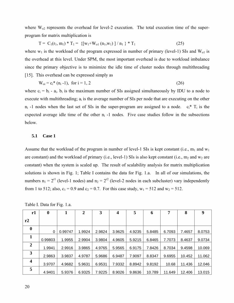
5.1 Case 1

Assume that the workload of the program in number of level-1 SIs is kept constant (i.e., m1 and w1

are constant) and the workload of primary (i.e., level-1) SIs is also kept constant (i.e., m2 and w2 are

constant) when the system is scaled up. The result of scalability analysis for matrix multiplication

solutions is shown in Fig. 1; Table I contains the data for Fig. 1.a. In all of our simulations, the

numbers n1 = 2r1 (level-1 nodes) and n2 = 2r2 (level-2 nodes in each subcluster) vary independently

from 1 to 512; also, c1 = 0.9 and c2 = 0.7. For this case study, w1 = 512 and w2 = 512.

Table I. Data for Fig. 1.a.

r1

r2

0 1 2 3 4 5 6 7 8 9

0 0 0.99747 1.9924 2.9824 3.9625 4.9235 5.8485 6.7093 7.4657 8.0753

1 0.99803 1.9955 2.9904 3.9804 4.9605 5.9215 6.8465 7.7073 8.4637 9.0734

2 1.9941 2.9916 3.9865 4.9765 5.9565 6.9175 7.8426 8.7034 9.4598 10.069

3 2.9863 3.9837 4.9787 5.9686 6.9487 7.9097 8.8347 9.6955 10.452 11.062

4 3.9707 4.9682 5.9631 6.9531 7.9332 8.8942 9.8192 10.68 11.436 12.046

5 4.9401 5.9376 6.9325 7.9225 8.9026 9.8636 10.789 11.649 12.406 13.015

21

6 5.8808 6.8783 7.8732 8.8632 9.8433 10.804 11.729 12.59 13.346 13.956

7 6.769 7.7665 8.7614 9.7514 10.731 11.692 12.617 13.478 14.235 14.844

8 7.5685 8.566 9.5609 10.551 11.531 12.492 13.417 14.278 15.034 15.644

9 8.2356 9.2331 10.228 11.218 12.198 13.159 14.084 14.945 15.701 16.311

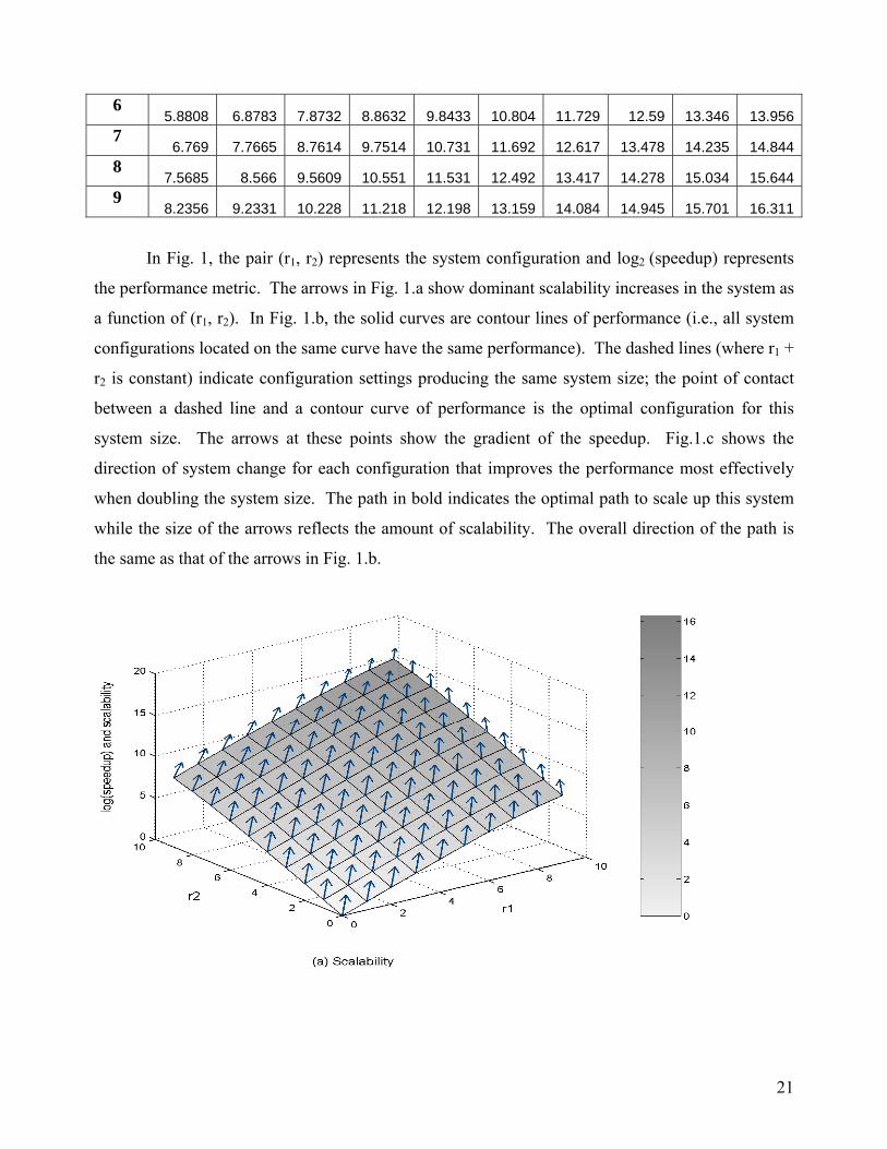
In Fig. 1, the pair (r1, r2) represents the system configuration and log2 (speedup) represents

the performance metric. The arrows in Fig. 1.a show dominant scalability increases in the system as

a function of (r1, r2). In Fig. 1.b, the solid curves are contour lines of performance (i.e., all system

configurations located on the same curve have the same performance). The dashed lines (where r1 +

r2 is constant) indicate configuration settings producing the same system size; the point of contact

between a dashed line and a contour curve of performance is the optimal configuration for this

system size. The arrows at these points show the gradient of the speedup. Fig.1.c shows the

direction of system change for each configuration that improves the performance most effectively

when doubling the system size. The path in bold indicates the optimal path to scale up this system

while the size of the arrows reflects the amount of scalability. The overall direction of the path is

the same as that of the arrows in Fig. 1.b.

22

Fig. 1. Scalability of a two-level cluster for matrix multiplication with fixed workload for the

program and level-1 SIs

5.2 Case 2

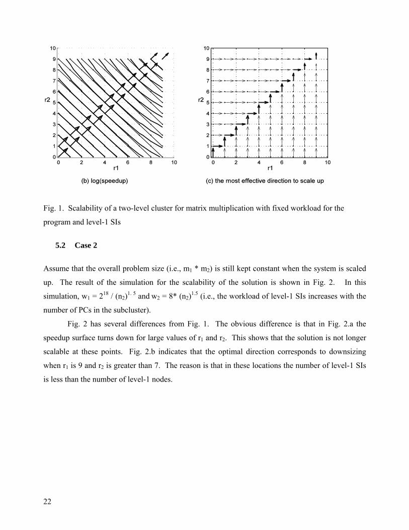
Assume that the overall problem size (i.e., m1 * m2) is still kept constant when the system is scaled

up. The result of the simulation for the scalability of the solution is shown in Fig. 2. In this

simulation, w1 = 218 / (n2)1. 5 and w2 = 8* (n2)1.5 (i.e., the workload of level-1 SIs increases with the

number of PCs in the subcluster).

Fig. 2 has several differences from Fig. 1. The obvious difference is that in Fig. 2.a the

speedup surface turns down for large values of r1 and r2. This shows that the solution is not longer

scalable at these points. Fig. 2.b indicates that the optimal direction corresponds to downsizing

when r1 is 9 and r2 is greater than 7. The reason is that in these locations the number of level-1 SIs

is less than the number of level-1 nodes.

23

Fig. 2. Scalability of a two-level cluster for matrix multiplication with fixed overall workload but

the workload of level-1 SIs increases with increases in the size of level-1 nodes

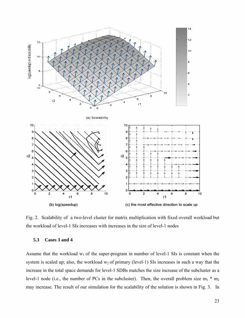
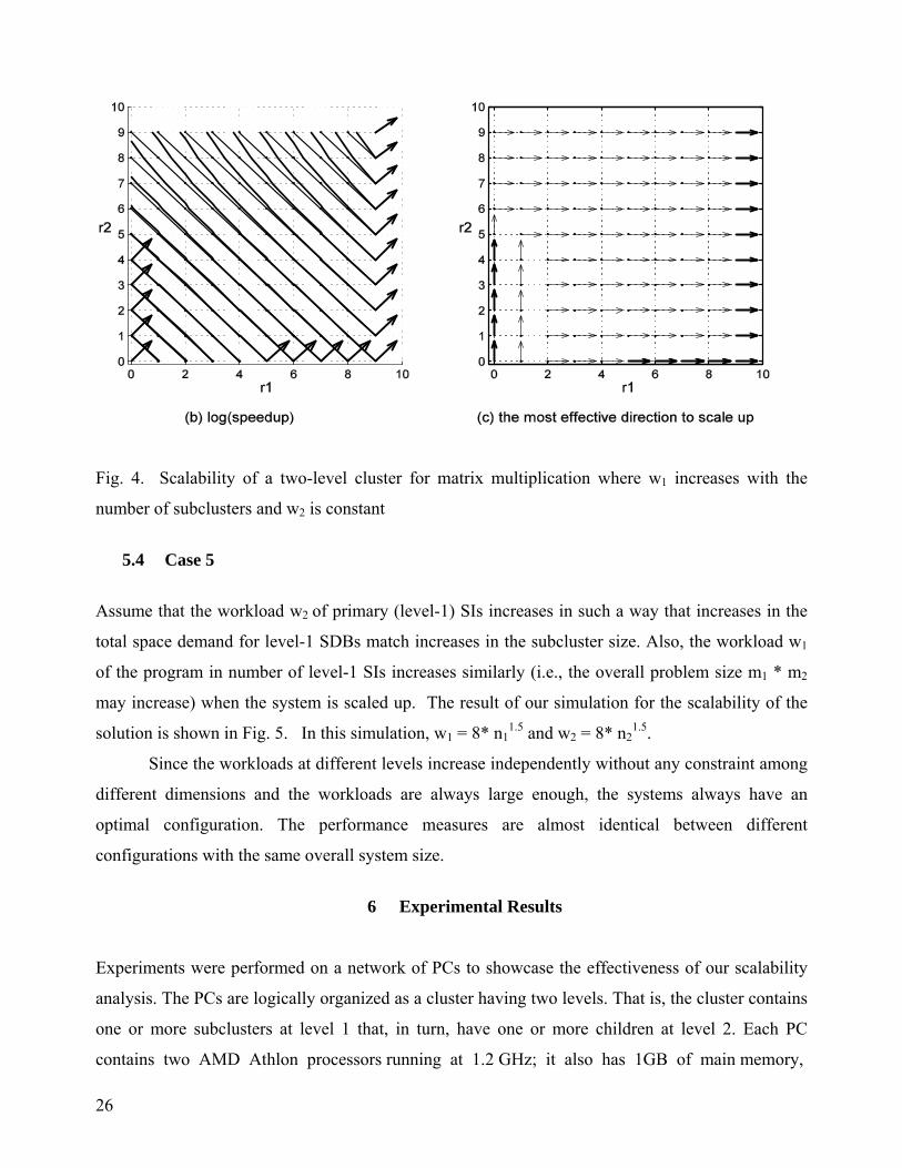
5.3 Cases 3 and 4

Assume that the workload w1 of the super-program in number of level-1 SIs is constant when the

system is scaled up; also, the workload w2 of primary (level-1) SIs increases in such a way that the

increase in the total space demands for level-1 SDBs matches the size increase of the subcluster as a

level-1 node (i.e., the number of PCs in the subcluster). Then, the overall problem size m1 * m2

may increase. The result of our simulation for the scalability of the solution is shown in Fig. 3. In

24

this simulation, w1 = 512 and w2 = 8* n21.5. Conversely, assume that the workload w2 of level-1 SIs

is constant, and w1 and the overall workload increase with the number of subcluster nodes in such

way that w2 = 512 and w1 = 8* n11.5. The corresponding result for the scalability of the solution is

shown in Fig. 4.

From Fig. 3 and Fig. 4, we can see that unlike the earlier cases, the optimal directions do not

form a path to help us find the global optimal configuration. In Fig. 3, among all the systems with r

= r1+r2 = 3, the optimal configuration is at (r1, r2) = (3, 0) and the local scalability vector is close to

(1, 1); the most effective direction to scale up a single dimension is (1, 0). However, the global

optimal configuration for the immediately next size (i.e., r = r1+r2 = 4) is at (0, 4). The same jump

is also observed in Fig. 4. This indicates that even if the starting point is optimal, we cannot find a

global optimal scaled up configuration by analyzing local scalability. The task of scaling up

hierarchical cluster systems for optimal solution is not then simple.

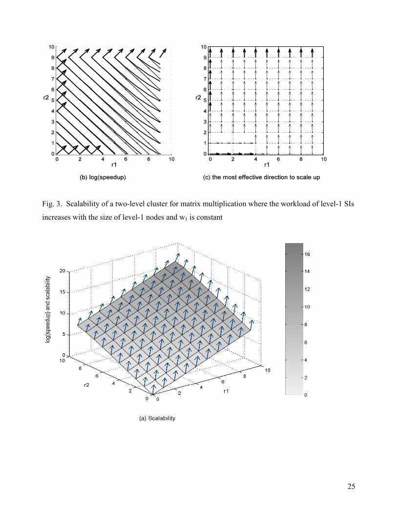
25

Fig. 3. Scalability of a two-level cluster for matrix multiplication where the workload of level-1 SIs

increases with the size of level-1 nodes and w1 is constant

26

Fig. 4. Scalability of a two-level cluster for matrix multiplication where w1 increases with the

number of subclusters and w2 is constant

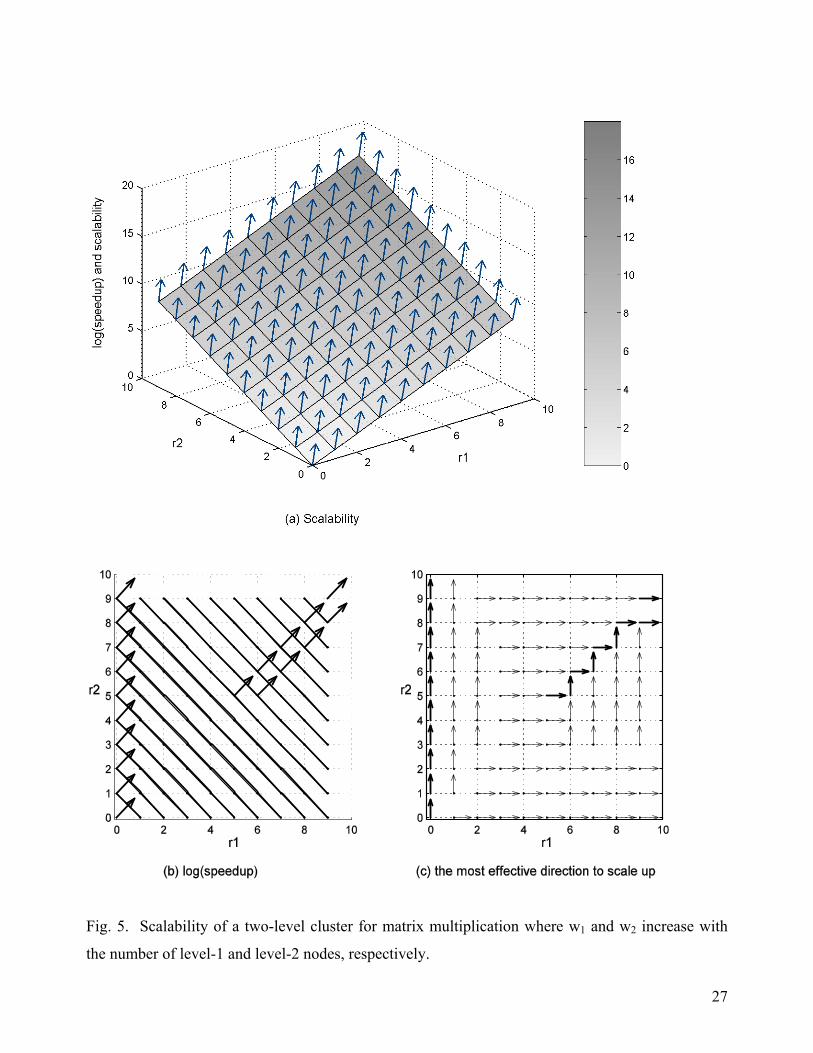
5.4 Case 5

Assume that the workload w2 of primary (level-1) SIs increases in such a way that increases in the

total space demand for level-1 SDBs match increases in the subcluster size. Also, the workload w1

of the program in number of level-1 SIs increases similarly (i.e., the overall problem size m1 * m2

may increase) when the system is scaled up. The result of our simulation for the scalability of the

solution is shown in Fig. 5. In this simulation, w1 = 8* n11.5 and w2 = 8* n2

1.5.

Since the workloads at different levels increase independently without any constraint among

different dimensions and the workloads are always large enough, the systems always have an

optimal configuration. The performance measures are almost identical between different

configurations with the same overall system size.

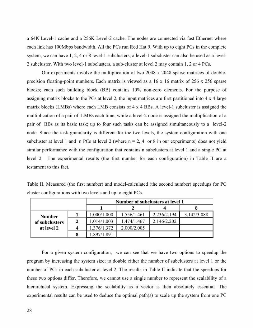
6 Experimental Results

Experiments were performed on a network of PCs to showcase the effectiveness of our scalability

analysis. The PCs are logically organized as a cluster having two levels. That is, the cluster contains

one or more subclusters at level 1 that, in turn, have one or more children at level 2. Each PC

contains two AMD Athlon processors running at 1.2 GHz; it also has 1GB of main memory,

27

Fig. 5. Scalability of a two-level cluster for matrix multiplication where w1 and w2 increase with

the number of level-1 and level-2 nodes, respectively.

28

a 64K Level-1 cache and a 256K Level-2 cache. The nodes are connected via fast Ethernet where

each link has 100Mbps bandwidth. All the PCs run Red Hat 9. With up to eight PCs in the complete

system, we can have 1, 2, 4 or 8 level-1 subclusters; a level-1 subcluster can also be used as a level-

2 subcluster. With two level-1 subclusters, a sub-cluster at level 2 may contain 1, 2 or 4 PCs.

Our experiments involve the multiplication of two 2048 x 2048 sparse matrices of double-

precision floating-point numbers. Each matrix is viewed as a 16 x 16 matrix of 256 x 256 sparse

blocks; each such building block (BB) contains 10% non-zero elements. For the purpose of

assigning matrix blocks to the PCs at level 2, the input matrices are first partitioned into 4 x 4 large

matrix blocks (LMBs) where each LMB consists of 4 x 4 BBs. A level-1 subcluster is assigned the

multiplication of a pair of LMBs each time, while a level-2 node is assigned the multiplication of a

pair of BBs as its basic task; up to four such tasks can be assigned simultaneously to a level-2

node. Since the task granularity is different for the two levels, the system configuration with one

subcluster at level 1 and n PCs at level 2 (where n = 2, 4 or 8 in our experiments) does not yield

similar performance with the configuration that contains n subclusters at level 1 and a single PC at

level 2. The experimental results (the first number for each configuration) in Table II are a

testament to this fact.

Table II. Measured (the first number) and model-calculated (the second number) speedups for PC

cluster configurations with two levels and up to eight PCs.

Number of subclusters at level 1 1 2 4 8

1 1.000/1.000 1.556/1.461 2.236/2.194 3.142/3.088 2 1.014/1.003 1.474/1.467 2.146/2.202 4 1.376/1.372 2.000/2.005

Number of subclusters

at level 2 8 1.897/1.891

For a given system configuration, we can see that we have two options to speedup the

program by increasing the system size; to double either the number of subclusters at level 1 or the

number of PCs in each subcluster at level 2. The results in Table II indicate that the speedups for

these two options differ. Therefore, we cannot use a single number to represent the scalability of a

hierarchical system. Expressing the scalability as a vector is then absolutely essential. The

experimental results can be used to deduce the optimal path(s) to scale up the system from one PC

29

up to eight PCs. It can be seen that the hierarchical system architecture and the chosen algorithm for

matrix multiplication collectively favor increases exclusively in the number of level-1 subclusters.

This is because the assignment of coarser grain tasks reduces the amount of data exchanges. We

have to emphasize here that the bandwidths are identical for inter-cluster and intra-cluster

communications in our system. If the network conditions were modified, the favor might shift but

the method to find the most effective path should not change.

Although this example uses experiments to evaluate performance, in the planning phases

(where the hardware is not available yet) the result should be derived by using a combination of

theory and possibly some small measurements. Models illustrating the behavior of scaling up a

system in a single dimension should not be difficult to derive. By combining such data and models,

the users should be able to obtain a multi-dimensional picture suitable for scalability analysis.

Let us now create a model for this two-level system and algorithm pair in an effort to

showcase our scalability analysis approach for this real-world problem. Based on the discussion in

Section 4.3, the problem complexities under SPM for level-1 and level-2 SIs are C1(r1, m1) = w1*

[1+ (r1-1) ∗ α1 /r1 + (r1-1) ∗ α2] / r1 and C2(r2, m2) = w2* [1+ (r2-1) ∗ β1 /r2 + (r2-1) ∗ β2] / r2,

respectively. The second and third terms to be added in the brackets represent the relative

communication overhead and relative unbalance overhead (appearing when some nodes are idle

after the last task has been assigned), respectively. The speedup is then given by

S = T(1,1)/T(r1, r2) = r1* r2/ {[1+ (r1-1) ∗ α1 /r1 + (r1-1) ∗ α2] *[1+ (r2-1) ∗ β1 /r2 + (r2-1) ∗ β2]}

From our experiments on the aforementioned two-level configurations, we can approximate

the values of the parameters by α1 = 0.3766, α2 = 0.1802, β1 = 1.418 and β2 = 0.2841. The

estimated speedups are then as shown in Table II (the second number for each configuration). It

becomes obvious that the estimated speedups approximate very well the experimental results.

Therefore, this simple performance model can aid us in choosing the right system, and our

scalability analysis is reliable and easy to carry out.

7 Conclusions

Scalability is an attribute characterizing hardware-software solutions. It does not solely depend on

either the target computer or the algorithm used to solve the respective problem. It depends on

many dimensions representing feature spaces for both. Current definitions of scalability can only

characterize partial features of a solution when the system and/or problem are scaled up. A

30

comprehensive scalability expression needs to use a vector as input. Each value in the vector relates

to a single feature change (i.e., a single dimension study). When mentioning scaled up solutions

with graceful performance, we must give the direction (i.e., resource) of change. For an optimally

configured multi-level cluster, the scalabilities at all the levels should be identical. However, a good

solution may not work well with the optimal configuration, especially if such a cluster is built as

general purpose. This is because the internal resources of PCs are not exchangeable. We cannot

increase the amount of a particular resource by decreasing another type of resource. A type of

resource may be over-equipped for a solution but be under-equipped for another solution.

Therefore, there is not any PC configuration in these dimensions that fits well all solutions and the

scalabilities in various dimensions may not be the same. Programs developed under SPM match

well the configurable features of multi-level PC clusters. The scalabilities of various levels can be

matched by reconfiguring the hierarchical structure. This approach guarantees that the efficiency

obtained is higher than a log-linear lower bound.

References

1. J.L. Gustafson, Reevaluating Amdahl’s Law, Comm. of ACM, Vol. 31(5), p18-21, May 1988

2. V. Kumar, A. Grama, A. Gupta, and G. Karypis, Introduction to Parallel Computing,

Redwood City, CA: Benjamin/Cummings Inc., 1994

3. D.R. Law, Scalable Means More than More: a Unifying Definition of Simulation Scalability,

Proc. 30th Conf. on Winter Simulation, p781-788, Washington, D.C., Dec. 1998.

4. M.D. Hill, What Is Scalability? ACM SIGARCH Computer Architecture News, Vol.18 (4),

p18-21, Dec. 1990.

5. D. Nussbaum and A. Agarwal, Scalability of Parallel Machines, Comm. of ACM, Vol.34(3),

p 57 – 61, Mar. 1991.

6. A. Sivasubramaniam, A. Singla, U. Ramachandran, and H. Venkateswaran, An Approach to

Scalability Study of Shared Memory Parallel Systems, ACM SIGMETRICS Performance

Evaluation Review, Vol.22(1), p171 – 180, May 1994.

31

7. J.S. Vetter and M.O. McCracken, Statistical Scalability Analysis of Communication

Operations in Distributed Applications, ACM SIGPLAN Notices, Vol.36 (7), p123 – 132,

June 2001.

8. R. Deters, Scalability and Information Agents, ACM SIGAPP Applied Computing

Review, Vol. 9 (3), p13-20, Sept. 2001.

9. G. Brataas and P. Hughes, Exploring Architectural Scalability, ACM SIGSOFT Software

Engineering Notes, Vol.29 (1), p125-129 Jan. 2004.

10. A.B. Bondi, Characteristics of Scalability and Their Impact on Performance, Proc. 2nd Int’l

workshop on Software and Performance, p195-203, Sept. 2000.

11. A.H. Karp and H.P. Flatt, Measuring Parallel Processor Performance, Comm. of ACM Vol.

33(5), p539-543, May 1990.

12. V. Kumar and V.N. Rao, Parallel Depth-First Search. Int’l J. of Parallel Programming Vol.

16(6), p501-519, June1987.

13. X-H. Sun and J.L. Gustafson, Towards a Better Parallel Performance Metric. Parallel

Computing, Vol. 17, p1093-1109, 1991.

14. M.D. Greenberg, Advanced Engineering Mathematics, New Jersey: Prentice-Hall, 1988.

15. D. Jin and S.G. Ziavras, A Super-Programming Approach for Mining Association Rules in

Parallel on PC Clusters, IEEE Trans. Paral. Distrib. Sys., Vol. 15(9), p783-794, Sept.

2004.

16. D. Jin and S.G. Ziavras, Modeling Distributed Data Representation and its Effect on Parallel

Data Accesses, Journal of Parallel and Distributed Computing, Special Issue on Design

and Performance of Networks for Super-, Cluster-, and Grid-Computing, Vol. 65(10),

p1281-1289, Oct. 2005.

17. D. Jin and S.G. Ziavras, A Super-Programming Technique for Large Sparse Matrix

Multiplication on PC Clusters, IEICE Trans. Information Systems, Vol. E87-D(7), p1774-

1781, July 2004.

32

18. S.G. Ziavras, On the Problem of Expanding Hypercube-Based Systems, Journal of Parallel

and Distributed Computing, Vol. 16(1), p41-53, Sept. 1992.

19. S.G. Ziavras, RH: A Versatile Family of Reduced Hypercube Interconnection Networks, IEEE

Trans. Paral. Distrib. Sys., Vol. 5(11), p1210-1220, Nov. 1994.

20. D.J. Mavriplis, M.J. Aftosmis and M. Berger, High Resolution Aerospace Applications Using

the NASA Columbia Supercomputer, International Journal of High Performance

Computing Applications, Vol. 21(1), p106-126, March 2007.

21. C.E. Goodyer and M. Berzins, Parallelization and Scalability Issues of a Multilevel

Elastohydrodynamic Lubrication Solver, Concurrency Computation Practice and

Experience, Vol. 19(4), p369-396, March 2007.

22. C. Engelmann and A. Geist, Super-scalable Algorithms for Computing on 100,000

Processors, Lecture Notes in Computer Science, Vol. 3514(I), p313-321, 2005.

23. B. Fang, Y. Deng and G. Martyna, Performance of the 3D FFT on the 6D Network Torus

QCDOC Parallel Supercomputer, Computer Physics Communications, Vol. 176(8),

p531-538, April 2007.

Appendix

Theorem: Assume an n-dimensional vector space V where for any vector v ∈ V we have v = ∑i=1n

(vi * ei ); vi, for i = 1, 2, …, n, is a non-negative real number and at least one of them is non-zero,

and {ei} form orthogonal normalized bases for this space. Also, assume a function E: V R that

maps a vector v in V to a real value in the real numbers domain R with E(v) = (v*u)/ (v*w); u and w

are two constant vectors in V (i.e., u = ∑i=1n

(ui * ei ) and w = ∑i=1n

(wi * ei )). Finally, xi = ui / wi.

1) If xk is the maximum value in the set {xi | i = 1, 2, …, n}, then for the vector y = xk * ek the

function E(y) yields the maximum value; i.e., E(y) ≥ E(v) for ∀ v ∈ V.

2) Assume that there exist multiple values xi in the set {xi | i = 1, 2, …, n} that are all equal to

the maximum value in this set (i.e., x s1 = x s2 = …= xsk > xs(k+1) … ≥ x s n and the indices {si

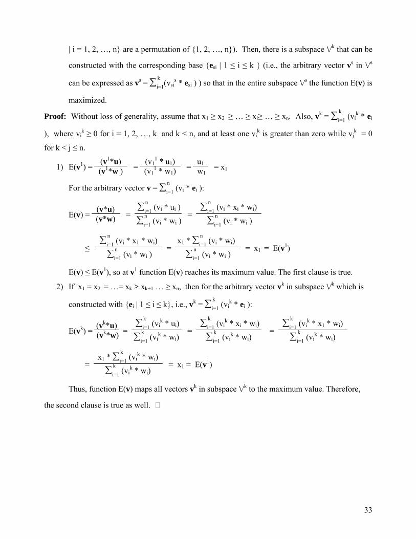
33

| i = 1, 2, …, n} are a permutation of {1, 2, …, n}). Then, there is a subspace Vk that can be

constructed with the corresponding base {esi | 1 ≤ i ≤ k } (i.e., the arbitrary vector vs in Vs

can be expressed as vs = ∑i=1k

(vsis * esi ) ) so that in the entire subspace Vs the function E(v) is

maximized.

Proof: Without loss of generality, assume that x1 ≥ x2 ≥ … ≥ xi≥ … ≥ xn. Also, vk = ∑i=1k

(vik * ei

), where vik ≥ 0 for i = 1, 2, …, k and k < n, and at least one vi

k is greater than zero while vjk = 0

for k < j ≤ n.

1) E(v1) = (v1*u)

(v1*w ) = (v1

1 * u1) (v1

1 * w1) = u1 w1 = x1

For the arbitrary vector v = ∑i=1n

(vi * ei ):

E(v) = (v*u)

(v*w) = ∑i=1

n (vi * ui )

∑i=1n

(vi * wi ) =

∑i=1n

(vi * xi * wi)

∑i=1n

(vi * wi )

≤ ∑i=1

n (vi * x1 * wi)

∑i=1n

(vi * wi ) =

x1 * ∑i=1n

(vi * wi)

∑i=1n

(vi * wi ) = x1 = E(v1)

E(v) ≤ E(v1), so at v1 function E(v) reaches its maximum value. The first clause is true.

2) If x1 = x2 = …= xk > xk+1 … ≥ xn, then for the arbitrary vector vk in subspace Vk which is

constructed with {ei | 1 ≤ i ≤ k}, i.e., vk = ∑i=1k

(vik * ei ):

E(vk) = (vk*u) (vk*w) =

∑i=1k

(vik * ui)

∑i=1k

(vik * wi)

= ∑i=1

k (vi

k * xi * wi)

∑i=1k

(vik * wi)

= ∑i=1

k (vi

k * x1 * wi)

∑i=1k

(vik * wi)

= x1 * ∑i=1

k (vi

k * wi)

∑i=1k

(vik * wi)

= x1 = E(v1)

Thus, function E(v) maps all vectors vk in subspace Vk to the maximum value. Therefore,

the second clause is true as well.