Embed Size (px)
Citation preview
HAL Id: tel-01191084https://tel.archives-ouvertes.fr/tel-01191084
Submitted on 1 Sep 2015
HAL is a multi-disciplinary open accessarchive for the deposit and dissemination of sci-entific research documents, whether they are pub-lished or not. The documents may come fromteaching and research institutions in France orabroad, or from public or private research centers.
L’archive ouverte pluridisciplinaire HAL, estdestinée au dépôt et à la diffusion de documentsscientifiques de niveau recherche, publiés ou non,émanant des établissements d’enseignement et derecherche français ou étrangers, des laboratoirespublics ou privés.
Robust nonlinear control : from continuous time tosampled-data with aerospace applications.
Giovanni Mattei
To cite this version:Giovanni Mattei. Robust nonlinear control : from continuous time to sampled-data with aerospaceapplications.. Automatic. Université Paris Sud - Paris XI, 2015. English. <NNT : 2015PA112025>.<tel-01191084>

UNIVERSITE PARIS SUD
ECOLE DOCTORALESciences et Technologie de l’Information, des Telecommunications
et des SystemesLaboratoire des Signaux et Systemes - L2S
DISCIPLINE: PHYSIQUE
THESE DE DOCTORAT
Soutenance prevue le 13/02/2015
par
Giovanni MATTEI
Robust Nonlinear Control
from continuous time to sampled-datawith aerospace applications
Composition du jury
Directeurs de these: Salvatore MONACO Professeur (DIAG, Sapienza)
Dorothee NORMAND-CYROT Directeur de recherche (L2S - Supelec)
Rapporteurs: Jean-Pierre BARBOT Professeur (ECS-Lab / ENSEA 6)
Giovanni ULIVI Professeur (DIA, Roma Tre)
Examinateurs: Stefano BATTILOTTI Professeur (DIAG, Sapienza)
Vincent FROMION Docteur (INRA Jouy-en-Josas)
Romeo ORTEGA Directeur de recherche (L2S - Supelec)
Membres invites: Silviu NICULESCU Directeur de recherche (L2S - Supelec)

This page intentionally left blank.

“I? What am I?” roared the President, and he rose slowly to an incredible height, like some
enormous wave about to arch above them and break. “You want to know what I am, do you?
Bull, you are a man of science. Grub in the roots of those trees and find out the truth about
them. Syme, you are a poet. Stare at those morning clouds. But I tell you this, that you will
have found out the truth of the last tree and the top-most cloud before the truth about me. You
will understand the sea, and I shall be still a riddle; you shall know what the stars are, and not
know what I am. Since the beginning of the world all men have hunted me like a wolf - kings
and sages, and poets and lawgivers, all the churches, and all the philosophies. But I have never
been caught yet, and the skies will fall in the time I turn to bay. I have given them a good run
for their money, and I will now.” (Sunday, ch.13)
G. K. Chesterton - The Man Who Was Thursday.
Science furthers ability, not knowledge. The value of having for a time rigorously pursued a
rigorous science does not derive precisely from the results obtained from it: for in relation to the
ocean of things worth knowing these will be a mere vanishing droplet. But there will eventuate
an increase in energy, in reasoning capacity, in toughness of endurance; one will have learned
how to achieve an objective by the appropriate means. To this extent it is invaluable, with regard
to everything one will afterwards do, once to have been a man of science.
F. Nietzsche - Human, All Too Human.

Abstract
The dissertation deals with the problems of stabilization and control of nonlinear systems with de-
terministic model uncertainties. First, in the context of uncertain systems analysis, we introduce
and explain the basic concepts of robust stability and stabilizability. Then, we propose a method
of stabilization via state-feedback in presence of unmatched uncertainties in the dynamics. The
recursive backstepping approach allows to compensate the uncertain terms acting outside the
control span and to construct a robust control Lyapunov function, which is exploited in the
subsequent design of a compensator for the matched uncertainties. The obtained controller is
called recursive Lyapunov redesign. Next, we introduce the stabilization technique through “Im-
mersion & Invariance” (I&I) as a tool to improve the robustness of a given nonlinear controller
with respect to unmodeled dynamics. The recursive Lyapunov redesign is then applied to the
attitude stabilization of a spacecraft with flexible appendages and to the autopilot design of an
asymmetric air-to-air missile. Contextually, we develop a systematic method to rapidly evaluate
the aerodynamic perturbation terms exploiting the deterministic model of the uncertainty. The
effectiveness of the proposed controller is highlighted through several simulations in the second
case-study considered. In the final part of the work, the technique of I&I is reformulated in the
digital setting in the case of a special class of systems in feedback form, for which constructive
continuous-time solutions exist, by means of backstepping and nonlinear domination arguments.
The sampled-data implementation is based on a multi-rate control solution, whose existence is
guaranteed for the class of systems considered. The digital controller guarantees, under sampling,
the properties of manifold attractivity and trajectory boundedness. The control law, computed
by finite approximation of a series expansion, is finally validated through numerical simulations
in two academic examples and in two case-studies, namely the cart-pendulum system and the
rigid spacecraft.
Keywords. Nonlinear control, robust control, robust control Lyapunov function, uncertainty
modeling, robust backstepping, Lyapunov redesign, recursive Lyapunov redesign, Immersion and
Invariance, nonlinear sampled data control, multi-rate control, missile autopilot design, attitude
stabilization, flexible spacecraft

List of the publications
1. Journals
• G. Mattei and S. Monaco - “Nonlinear Autopilot Design for an Asymmetric
Missile Using Robust Backstepping Control” - Journal of Guidance, Control,
and Dynamics, (2014), doi: http://arc.aiaa.org/doi/abs/10.2514/1.G000434.
2. Conferences
• G. Mattei and S. Monaco - “Nonlinear Robust Autopilot for Rolling and
Lateral Motions of an Aerodynamic Missile” - AIAA GNC Conference 2012
- 4467.
• G. Mattei and S. Monaco - “Robust Backstepping Control of Missile Lateral
and Rolling Motions in the Presence of Unmatched Uncertainties” - IEEE
CDC 2012 - p. 2878-2883.
• G. Mattei, P. Di Giamberardino, S. Monaco, M.D. Normand-Cyrot - “Lya-
punov Based Attitude Stabilization of an Underactuated Spacecraft with
Flexibilities” - IAA-AAS DyCoSS2 2014 - 140703.
• G. Mattei, A. Carletti, P. Di Giamberardino, S. Monaco, M.D. Normand-
Cyrot - “Adaptive Robust Redesign of Feedback Linearization for a Satellite
with Flexible Appendages” - IAA-AAS DyCoSS2 2014 - 141007.
• G. Mattei, S. Monaco, M.D. Normand-Cyrot - “Multi-rate sampled-data I&I
stabilization of a class of nonlinear systems” - IEEE ECC 2015 proceedings.
• G. Mattei, S. Monaco, M.D. Normand-Cyrot - “Robust Nonlinear Attitude
Stabilization of a Spacecraft through Digital Implementation of an I&I Sta-
bilizer” - IFAC MICNON 2015 proceedings.
3. Technical reports
• G. Mattei and F. Liberati - “Modelli di option pricing: l’equazione di Black &
Scholes” - Department of Computer, Control, and Management Engineering
“Antonio Ruberti” Technical Reports, Report n. 11, 2013.

Ringraziamenti
Questo lavoro e il frutto di tre anni intensi di studio e ricerca, successi e buchi nell’acqua,
centinaia di simulazioni in Matlab & Simulink, nottate in bianco, conferenze in America
e Europa. Tre anni trascorsi a meta fra Roma e Parigi, grazie all’opportunita della
cotutela per la quale ringrazio con tutto il cuore i miei due mentori, il Professor Monaco
e la Professoressa Normand-Cyrot, i quali mi hanno saputo guidare, saggiamente con-
sigliare e intelligentemente indirizzare in questo percorso che giunge a conclusione. Loro
hanno saputo costantemente alimentare la mia “fame di Automatica”, stimolando con-
tinuamente il mio interesse e la mia curiosita, anche sui terreni piu ostici.
Un grazie speciale va ai miei genitori, i quali mi hanno sempre incoraggiato in ogni mia
decisione e che mi continuano a sostenere nonostante la distanza. La mia partenza per
Parigi non e stata facile da affrontare per loro, ma nonostante tutto mi sono sempre
vicini col loro amore incondizionato. Voglio inoltre ringraziare i fratelloni Emanuele
e Paolo e le loro mogli Cristina e Federica per avermi sempre supportato. Non finiro
mai di ringraziarvi per avermi reso zio di un “nipotame” incredibile. Grazie mille a
Monica, Maria, Beatrice, Tommaso, Filippo, Michele, Caterina e Francesco. Voglio poi
ringraziare zio Alfredo e zia Lella per avermi sopportato e per i vari viaggi in aeroporto
che mi avete risparmiato, voglio bene anche a voi sebbene in certi casi non si direbbe.
Grazie anche a Michele e Lamberto per la continua brit-inspiration e per le serate allo
Scholars Lounge a sentire i Radio Supernova. Grazie a Maria e Emanuele per la speranza,
alle gemelle Agnese e Benedetta per la pazienza e a zio Guido e zia Teresa per il loro
supporto.
Grazie ad Alice, per il suo immenso amore e la sua infinita pazienza.
Grazie a Daniele per le chiacchierate di Automatica e i consigli e a Riccardo, perche
anche se ormai ci sentiamo pochissimo e sempre un grande piacere. Grazie a Simone
perche in fondo la scelta e Automatica, a Michele per le partite della Roma viste a
casa sua nel Marais, al Braciola per il calciotto della domenica, a Lorenzo anche se
e della juve e a Raffaele per il pogo al suo matrimonio. Grazie a Damiano per la
sua costante presenza e ad Andrea & Laura per le partite a tresette. Grazie infine a
tutti quelli che hanno reso indimenticabile questo ultimo anno di dottorato: Fabrizio &
Giuliano, Matteo & Matteo, Irene, Ariannona, Chiara, Laura, Silvia, Miguel, Vincenzo,
Francesco, Gianpaolo, Raffaello, Ugo & Mario, Antonio, Gabriele per i Beady Eye al
Bataclan, Federico & Giacomo & Valerio & Luca per le serate brit, Dario per esserci
sempre stato e Andrea, perche mi ricordi me ai tempi della laurea specialistica.
v

But the little things they make me so happy
All I want to do is live by the sea
Little things they make me so happy
But it’s good, yes it’s good . . . it’s good to be free.

Contents
Abstract iii
List of the publications iv
Ringraziamenti v
Contents vii
List of Figures x
List of Tables xiii
Symbols xiv
Introduction 1
1 Robust stability and stabilizability of nonlinear systems 9
1.1 Lyapunov stability of uncertain systems . . . . . . . . . . . . . . . . . . . 9
1.1.1 Semiglobal and practical stability . . . . . . . . . . . . . . . . . . . 13
1.1.2 Input-to-state stability . . . . . . . . . . . . . . . . . . . . . . . . . 15
1.2 Control Lyapunov Function . . . . . . . . . . . . . . . . . . . . . . . . . . 16
1.3 Robust nonlinear stabilization . . . . . . . . . . . . . . . . . . . . . . . . . 23
1.3.1 Nonlinear uncertain systems . . . . . . . . . . . . . . . . . . . . . . 23
1.3.2 Practical-robust stability and stabilizability . . . . . . . . . . . . . 24
1.3.3 Robust Control Lyapunov Function . . . . . . . . . . . . . . . . . 27
1.3.3.1 RCLF in absence of disturbance input . . . . . . . . . . . 29
1.3.3.2 RCLF implies robust stabilizability . . . . . . . . . . . . 30
1.3.3.3 Small control property . . . . . . . . . . . . . . . . . . . . 31
1.3.3.4 Robust stabilizability implies RCLF . . . . . . . . . . . . 31
2 Structure of an uncertain nonlinear system 33
2.1 Uncertainty representation . . . . . . . . . . . . . . . . . . . . . . . . . . . 34
2.2 Input-affine nonlinear uncertain systems . . . . . . . . . . . . . . . . . . . 38
2.2.1 Examples of unstabilizable uncertain systems . . . . . . . . . . . . 39
2.2.2 Matching conditions . . . . . . . . . . . . . . . . . . . . . . . . . . 41
2.2.3 Generalized matching conditions . . . . . . . . . . . . . . . . . . . 42
vii

Contents viii
2.3 Uncertainty modeling . . . . . . . . . . . . . . . . . . . . . . . . . . . . . 44
3 Robust nonlinear control design 50
3.1 Lyapunov redesign revisited . . . . . . . . . . . . . . . . . . . . . . . . . . 50
3.2 Robust Backstepping . . . . . . . . . . . . . . . . . . . . . . . . . . . . . . 54
3.3 Recursive Lyapunov redesign . . . . . . . . . . . . . . . . . . . . . . . . . 57
3.4 Stabilization via Immersion & Invariance . . . . . . . . . . . . . . . . . . 59
3.4.1 The class of systems under study . . . . . . . . . . . . . . . . . . . 61
3.4.2 Control design . . . . . . . . . . . . . . . . . . . . . . . . . . . . . 62
4 Attitude stabilization of a flexible spacecraft 65
4.1 Dynamic model . . . . . . . . . . . . . . . . . . . . . . . . . . . . . . . . . 65
4.2 Control design . . . . . . . . . . . . . . . . . . . . . . . . . . . . . . . . . 68
4.2.1 Robust backstepping . . . . . . . . . . . . . . . . . . . . . . . . . . 69
4.2.2 Recursive Lyapunov redesign . . . . . . . . . . . . . . . . . . . . . 74
5 Missile autopilot design 77
5.1 Dynamic model . . . . . . . . . . . . . . . . . . . . . . . . . . . . . . . . . 77
5.1.1 Modeling for nominal control . . . . . . . . . . . . . . . . . . . . . 83
5.1.2 Modeling for robust control . . . . . . . . . . . . . . . . . . . . . . 84
5.2 Control design . . . . . . . . . . . . . . . . . . . . . . . . . . . . . . . . . 91
5.2.1 Control objectives . . . . . . . . . . . . . . . . . . . . . . . . . . . 91
5.2.2 Nominal control law . . . . . . . . . . . . . . . . . . . . . . . . . . 93
5.2.3 Robust nonlinear control . . . . . . . . . . . . . . . . . . . . . . . . 94
5.3 Simulation and results . . . . . . . . . . . . . . . . . . . . . . . . . . . . . 102
5.3.1 Skid-To-Turn maneuver . . . . . . . . . . . . . . . . . . . . . . . . 102
5.3.2 Bank-To-Turn maneuver . . . . . . . . . . . . . . . . . . . . . . . . 106
6 Immersion and Invariance under sampling 111
6.1 Sampled-data I&I control design . . . . . . . . . . . . . . . . . . . . . . . 112
6.1.1 Sampled-data equivalent models . . . . . . . . . . . . . . . . . . . 112
6.1.2 Main result . . . . . . . . . . . . . . . . . . . . . . . . . . . . . . . 113
6.1.3 Sampled-data approximate design . . . . . . . . . . . . . . . . . . 115
6.1.3.1 Single-rate solution . . . . . . . . . . . . . . . . . . . . . 115
6.1.3.2 Multi-rate solution . . . . . . . . . . . . . . . . . . . . . . 116
6.2 Example with single-rate control . . . . . . . . . . . . . . . . . . . . . . . 117
6.3 Example with multi-rate control . . . . . . . . . . . . . . . . . . . . . . . 120
6.4 The cart-pendulum system . . . . . . . . . . . . . . . . . . . . . . . . . . 123
7 Robust attitude stabilization via digital I&I 128
7.1 Introduction . . . . . . . . . . . . . . . . . . . . . . . . . . . . . . . . . . . 128
7.2 Spacecraft dynamic modeling . . . . . . . . . . . . . . . . . . . . . . . . . 129
7.3 Immersion and Invariance stabilization . . . . . . . . . . . . . . . . . . . . 130
7.3.1 Recalls . . . . . . . . . . . . . . . . . . . . . . . . . . . . . . . . . . 130
7.3.2 The class of systems under study . . . . . . . . . . . . . . . . . . . 132
7.3.3 Problem setting . . . . . . . . . . . . . . . . . . . . . . . . . . . . . 133
7.4 Sampled-data control design . . . . . . . . . . . . . . . . . . . . . . . . . . 134
7.5 Attitude stabilization of the rigid spacecraft . . . . . . . . . . . . . . . . . 136

Contents ix
7.5.1 Continuous-time control design . . . . . . . . . . . . . . . . . . . . 136
7.5.2 Sampled-data control design . . . . . . . . . . . . . . . . . . . . . . 138
7.5.3 Simulations . . . . . . . . . . . . . . . . . . . . . . . . . . . . . . . 139
7.6 Concluding remarks . . . . . . . . . . . . . . . . . . . . . . . . . . . . . . 143
Conclusions and perspectives 144
Resume 147
Notation 148
Bibliography 150
List of Figures
1.1 Nonlinear robust control paradigm. . . . . . . . . . . . . . . . . . . . . . . 25
3.1 Sigmoidal function represented for three different values of the slope. . . . 53
4.1 Artist’s impression of the lander Beagle2 leaving the orbiter Mars Express(courtesy of ESA) c©. . . . . . . . . . . . . . . . . . . . . . . . . . . . . . . 66
4.2 The nonlinear GES kinematic sub-system cascaded with the linear GESflexible sub-system yields a nonlinear GES cascade. . . . . . . . . . . . . . 71
5.1 Meteor is an active radar guided beyond-visual-range air-to-air missile(BVRAAM) being developed by MBDA missile systems. Meteor will offer amulti-shot capability against long range manoeuvring targets in a heavyelectronic countermeasures (ECM) environment with range in excess of100km. The picture is taken from defenseindustrydaily.com, all rightsreserved c©. . . . . . . . . . . . . . . . . . . . . . . . . . . . . . . . . . . . 78
5.2 STT maneuver - Angle of Attack tracking response at two different levelsof uncertainty: nominal controller. . . . . . . . . . . . . . . . . . . . . . . 103
5.3 STT maneuver - Angle of Sideslip tracking response at two different levelsof uncertainty: nominal controller. . . . . . . . . . . . . . . . . . . . . . . 103
5.4 STT maneuver - Bank Angle regulation response at two different levelsof uncertainty: nominal controller. . . . . . . . . . . . . . . . . . . . . . . 103
5.5 STT maneuver - Norm of the control inputs vector at two different levelsof uncertainty: nominal controller. . . . . . . . . . . . . . . . . . . . . . . 104
5.6 STT maneuver - Angle of Attack tracking response at two different levelsof uncertainty: robust controller. . . . . . . . . . . . . . . . . . . . . . . . 104
5.7 STT maneuver - Angle of Sideslip tracking response at two different levelsof uncertainty: robust controller. . . . . . . . . . . . . . . . . . . . . . . . 105
5.8 STT maneuver - Bank Angle regulation response at two different levelsof uncertainty: robust controller. . . . . . . . . . . . . . . . . . . . . . . . 105
5.9 STT maneuver - Norm of the control inputs vector at two different levelsof uncertainty: robust controller. . . . . . . . . . . . . . . . . . . . . . . . 105
5.10 STT maneuver - Norm of the tracking error vector and energy of thecontrol inputs vector at low uncertainty: comparison between nominaland robust controllers . . . . . . . . . . . . . . . . . . . . . . . . . . . . . 106
5.11 STT maneuver - Norm of the tracking error vector and energy of thecontrol inputs vector at high uncertainty: comparison between nominaland robust controllers . . . . . . . . . . . . . . . . . . . . . . . . . . . . . 106
5.12 BTT maneuver - Angle of Attack tracking response at two different levelsof uncertainty: nominal controller. . . . . . . . . . . . . . . . . . . . . . . 107
x
List of Figures xi
5.13 BTT maneuver - Angle of Sideslip regulation response at two differentlevels of uncertainty: nominal controller. . . . . . . . . . . . . . . . . . . . 107
5.14 BTT maneuver - Bank Angle tracking response at two different levels ofuncertainty: nominal controller. . . . . . . . . . . . . . . . . . . . . . . . . 108
5.15 BTT maneuver - Norm of the control inputs vector at two different levelsof uncertainty: nominal controller. . . . . . . . . . . . . . . . . . . . . . . 108
5.16 BTT maneuver - Angle of Attack tracking response at two different levelsof uncertainty: robust controller. . . . . . . . . . . . . . . . . . . . . . . . 108
5.17 BTT maneuver - Angle of Sideslip regulation response at two differentlevels of uncertainty: robust controller. . . . . . . . . . . . . . . . . . . . . 109
5.18 BTT maneuver - Bank Angle tracking response at two different levels ofuncertainty: robust controller. . . . . . . . . . . . . . . . . . . . . . . . . . 109
5.19 BTT maneuver - Norm of the control inputs vector at two different levelsof uncertainty: robust controller. . . . . . . . . . . . . . . . . . . . . . . . 109
5.20 BTT maneuver - Norm of the tracking error vector and energy of thecontrol inputs vector at low uncertainty: comparison between nominaland robust controllers . . . . . . . . . . . . . . . . . . . . . . . . . . . . . 110
5.21 BTT maneuver - Norm of the tracking error vector and energy of thecontrol inputs vector at high uncertainty: comparison between nominaland robust controllers . . . . . . . . . . . . . . . . . . . . . . . . . . . . . 110
6.1 x1 evolutions and comparison with the target system when δ = 0.2 s. Inblack the target system, in red the continuous-time evolution, in blue theevolution under ud and in green that under ud0. . . . . . . . . . . . . . . . 118
6.2 x2 evolutions when δ = 0.2 s. In red the continuous-time evolution, inblue the evolution under ud and in green that under ud0. . . . . . . . . . . 118
6.3 u when δ = 0.2 s. In red the continuous-time input, in blue ud and ingreen ud0. . . . . . . . . . . . . . . . . . . . . . . . . . . . . . . . . . . . . 118
6.4 x1 evolutions and comparison with the target system when δ = 0.8 s. Inblack the target system, in red the continuous-time evolution, in blue theevolution under ud and in green that under ud0. . . . . . . . . . . . . . . . 119
6.5 x2 evolutions when δ = 0.8 s. In red the continuous-time evolution, inblue the evolution under ud and in green that under ud0. . . . . . . . . . . 119
6.6 u when δ = 0.8 s. In red the continuous-time input, in blue ud and ingreen ud0. . . . . . . . . . . . . . . . . . . . . . . . . . . . . . . . . . . . . 119
6.7 x1 evolutions and comparison with the target system when δ = 0.05 s. Inblack the target system, in red the continuous-time evolution, in blue theevolution under multi-rate and in green that under ud10 − ud20. . . . . . . 121
6.8 x2 and x3 evolutions when δ = 0.05 s. In red the continuous-time evo-lution, in blue the evolution under multi-rate and in green that underud10 − ud20. . . . . . . . . . . . . . . . . . . . . . . . . . . . . . . . . . . . 122
6.9 u when δ = 0.05 s. In red the continuous-time input, in blue the multi-rate and in green the emulated. . . . . . . . . . . . . . . . . . . . . . . . . 122
6.10 x1 evolutions and comparison with the target system when δ = 0.1 s. Inblack the target system, in red the continuous-time evolution, in blue theevolution under multi-rate and in green that under ud10 − ud20. . . . . . . 122
6.11 x2 and x3 evolutions when = δ = 0.1 s. In red the continuous-timeevolution, in blue the evolution under multi-rate and in green that underud10 − ud20. . . . . . . . . . . . . . . . . . . . . . . . . . . . . . . . . . . . 123

List of Figures xii
6.12 u when δ = 0.1 s. In red the continuous-time input, in blue the multi-rateand in green the emulated. . . . . . . . . . . . . . . . . . . . . . . . . . . . 123
6.13 Pendulum heading angle w.r.t. the vertical, comparison between continu-ous (red) and sampled-data controllers (emulated in green and first orderin blue) at T = 0.1 s . . . . . . . . . . . . . . . . . . . . . . . . . . . . . 125
6.14 Pendulum angular velocity, comparison between continuous (red) andsampled-data controllers (emulated in green and first order in blue) atT = 0.1 s . . . . . . . . . . . . . . . . . . . . . . . . . . . . . . . . . . . . 125
6.15 Cart velocity trajectory, comparison between continuous (red) and sampled-data controllers (emulated in green and first order in blue) at T = 0.1s . . . . . . . . . . . . . . . . . . . . . . . . . . . . . . . . . . . . . . . . . 126
6.16 Control input, comparison between continuous (red) and sampled-datacontrollers (emulated in green and first order in blue) at T = 0.1 s . . . . 126
6.17 Pendulum heading angle w.r.t. the vertical, comparison between continu-ous (red) and sampled-data controllers (emulated in green and first orderin blue) at T = 0.3 s . . . . . . . . . . . . . . . . . . . . . . . . . . . . . 126
6.18 Pendulum angular velocity, comparison between continuous (red) andsampled-data controllers (emulated in green and first order in blue) atT = 0.3 s . . . . . . . . . . . . . . . . . . . . . . . . . . . . . . . . . . . . 127
6.19 Cart velocity trajectory, comparison between continuous (red) and sampled-data controllers (emulated in green and first order in blue) at T = 0.3s . . . . . . . . . . . . . . . . . . . . . . . . . . . . . . . . . . . . . . . . . 127
6.20 Control input, comparison between continuous (red) and sampled-datacontrollers (emulated in green and first order in blue) at T = 0.3 s . . . . 127
7.1 T = 0.2 s Modified CR parameters trajectories ρ(t). . . . . . . . . . . . 140
7.2 T = 0.2 s Angular velocities trajectories ω(t). . . . . . . . . . . . . . . . 140
7.3 T = 0.2 s Torques trajectories τ(t). . . . . . . . . . . . . . . . . . . . . . 140
7.4 T = 0.2 s z(t) trajectories. . . . . . . . . . . . . . . . . . . . . . . . . . . 141
7.5 T = 0.2 s Control inputs trajectories u(t). . . . . . . . . . . . . . . . . . 141
7.6 T = 0.5 s Modified CR parameters trajectories ρ(t). . . . . . . . . . . . 141
7.7 T = 0.5 s Angular velocities trajectories ω(t). . . . . . . . . . . . . . . . 142
7.8 T = 0.5 s Torques trajectories τ(t). . . . . . . . . . . . . . . . . . . . . . 142
7.9 T = 0.5 s z(t) trajectories. . . . . . . . . . . . . . . . . . . . . . . . . . . 142
7.10 T = 0.5 s Control inputs trajectories u(t). . . . . . . . . . . . . . . . . . 143

List of Tables
5.1 Missile airframe parameters . . . . . . . . . . . . . . . . . . . . . . . . . . 102
7.1 Inertia moments . . . . . . . . . . . . . . . . . . . . . . . . . . . . . . . . 139
xiii

Symbols
Asymmetric missile parameters
m mass of the missile kg
Ix, Iy, Iz, Ixz moments of inertia kg· m2
d diameter of the fuselage m
S cross-sectional area m2
xb, yb, zb unit-vectors of body-axes m
ϕ, α, β bank, attack and sideslip angles rad
p, q, r angular velocities rad· s−1
δR, δP , δY overall tail-fins angular deflections rad
Fy, Fz aerodynamic forces N
Mx, My, Mz aerodynamic moments N·mρ air density kg· m−3
M Mach number -
Vm, Vs missile velocity and speed of sound m/s12ρV
2m dynamic pressure Qd kg·m−1s−2
CNy, CNz aerodynamic coefficients (forces) -
Cl, Cm, Cn aerodynamic coefficients (moments) -
Gp, Gq, Gr aerodynamic coefficients (control deflections) -
ayi, byi i = 1, . . . , 4 parameters defining Fy -
azi, bzi i = 1, . . . , 4 parameters defining Fz -
di i = 1, . . . , 5 parameters defining Mx -
mi i = 1, . . . , 4 parameters defining My -
ni i = 1, . . . , 4 parameters defining Mz -
Clp stability derivative of the rolling moment -
Cmα , Cmαβ , Cmq , Cnpβ stability derivatives of the pitching moment -
Cnβ , Cnαβ , Cnr , Cnpα , CnδY stability derivatives of the yawing moment -
Cmi, i = 1, 2, 3, 4 parameters defining the Magnus effect s−1/-
τ time constant of the actuators dynamics s
I3 three-dimensional identity matrix s
xiv
Dedicated to my beloved parents, Virginio and Anna Maria.
xv

Introduction
Automatic control design of nonlinear systems affected by disturbances and model un-
certainties is a central topic of interest for the whole scientific community involved in
feedback control system analysis and synthesis. In the present work, we develop a proce-
dure to achieve practical asymptotic stabilization of nonlinear systems with matched and
unmatched uncertainties, mostly representing modeling errors in the parameters of the
system and time-varying disturbances. The core idea is to unify the existing results of
Lyapunov redesign and robust backstepping into a single stabilizing controller, which we
call recursive Lyapunov redesign. This tool merges the multi-step philosophy of robust
backstepping with the implicit control definition of Lyapunov redesign to counteract the
effects of both matched and unmatched uncertainties in system dynamics. The property
of stability which can be achieved is that of practical robust global asymptotic stability,
meaning that the closed-loop trajectories converge to an arbitrarily shrinkable com-
pact set surrounding the origin. Such an approach results particularly suited to design
control laws for aerospace systems, whose dynamics is usually highly nonlinear, with
time-varying uncertain parameters and disturbances. We apply the proposed technique
to two case studies, the attitude stabilization of a spacecraft with flexible appendages
and the autopilot design for an asymmetric tail-controlled air-to-air missile.
The construction of a nonlinear stabilizing controller working in the presence of system
uncertainties of various nature has captured the attention of control scientists since the
early Eighties, starting from linear systems with matched uncertainties [21, 41, 70], next
relaxing the matching conditions [8, 9] and finally approaching nonlinear systems [22]
and the application to chemical processes [64]. However, it was only in the early Nineties
that constructive solutions of robust controllers for nonlinear systems started to appear
in the literature, beginning with the work of Isidori and Astolfi [54], mainly devoted
to the problem of disturbance attenuation in the nonlinear H∞ setting. The robust
backstepping approach was first introduced in 1993 by Freeman and Kokotovic [31]
and by Marino and Tomei [81], from different points of view. A similar construction,
however, was found one year before, in 1992, by Qu in [103]. In the following years,
the techniques became more and more refined and several important results on robust
1
Introduction 2
nonlinear stabilization were obtained [32, 59, 104, 105], also paving the way for the
publication of two fundamental books in the field, the first by Freeman and Kokotovic
[36] and the second by Qu [106]. Depending on applications, design constraints and
methodological improvements, the original core ideas have been progressively specialized
and detailed into different areas of interest, like robust adaptive nonlinear control [33,
56, 102, 107], output feedback stabilization and observer design [3, 11–13, 79, 80, 122],
saturated feedback problems [34, 123], inverse optimality results [35, 100] and so on.
New successful concepts were also developed struggling in making a nonlinear control
system robustly stable with respect to external disturbances, one and for all Input-
to-State Stability (ISS) [117], with all her friends and cousins, for instance integral
Input-to-State Stability (iISS) [2], set Input-to-State Stability [39], incremental stability
[1], incremental norm [38] and contraction theory [75]. We cannot keep from mentioning
sliding modes. The old idea of sliding surface and the corresponding sliding mode
control laws represent the simplest tools guaranteeing robust nonlinear stabilization
[128]. They have the advantage of ensuring a finite-time convergence on the surface
where the desired behavior of the system is enforced. However, the discontinuity of the
control laws obtained may cause serious implementation issues, one for all the problem
of “chattering”. A solution has been proposed with higher-order sliding modes, which
involve a dynamic extension of the system [10, 30]. Sliding mode control theory and its
applications have been explored high and low during the years, with modifications of
the original to improve robustness and embrace a broader class of uncertain systems.
Notable extensions of the theory lead to sliding-mode observer designs via the super-
twisting algorithm [29] and other applications to the measurements feedback case [71].
The basic ideas exploited in robust backstepping design to counteract the effect of the
unmatched uncertainties are those of recursion and virtual control. Moreover, this tech-
nique provides a systematic way of construction of a control Lyapunov functions for
systems in pure-feedback or strict-feedback form. These ideas were already introduced,
although in an embryonic form, in the work of Feuer and Morse [28]. Later, they were
developed simultaneously by Byrnes and Isidori [15], Kokotovic, Sontag and Sussmann
[63, 120] and further refined by Tsinias in the early Nineties [125]. In the Nineties,
these ideas were also deeply exploited in adaptive controller design and revealed them-
selves to be particularly suited in several application domains, as widely shown in [60]
and in the book by Krstic, Kanellakopoulos and Kokotovic [65]. In the following years,
the ideas of backstepping were extended to different system structures. The forwarding
technique was introduced to construct nonlinear stabilizer for systems in feedforward
form [55, 89, 111], while the interlacing technique to stabilize systems in interlaced form
[73, 112]. The reader should be warned with the fact that some of this ideas were al-
ready introduced, under slightly different forms, in the most cited book in the control

Introduction 3
literature by Alberto Isidori [52], and further developed in [53].
The design of robust controllers for nonlinear systems arouses the interest of the aerospace
community, since most of the physical systems in the aerospace domain present nonlinear
and uncertain dynamics. Let us consider, for instance, the problem of missile autopilot
design, which concerns highly nonlinear dynamics with uncertain, rapidly varying, pa-
rameters. Starting from the late Seventies the problem has been faced using classical and
Linear Quadratic regulators based upon dynamical models linearized around fixed oper-
ating points. These methods lead naturally to the design of several linear time-invariant
(LTI) point-regulators around equilibria defined on stationary conditions, usually involv-
ing Mach number, altitude and weight. The controller, resulting from the interpolation
of the fixed-point regulators, guarantees global stability only in the case of slowly varying
conditions on both the states and the parameters. This technique, named gain schedul-
ing, still represents the state-of-the-art in control system design for missile autopilots;
this is mostly due to the simplicity of implementation of gain-scheduled regulators, which
also ensure relatively good performance. Classical gain scheduling design are presented,
for instance, in [98] and [40]. In the Nineties, extensions of these techniques brought
several improvements, like guaranteed stability margins and performance levels ([113],
[99], [7], [109] and references therein). Robustness issues have also been addressed using
suitable extensions of H∞ techniques in [37] and [38]. The breakthrough of LPV (lin-
ear parameter-varying) and quasi-LPV approaches in the last two decades has guided
the research and the designers towards new, more systematic and rigorous methodolo-
gies. Main features of these new approaches are the sounder robustness/performance
criteria used and the simplified control synthesis process adopted. The price to pay,
especially for quasi-LPV controllers, is an increased level of conservatism due to the
non-uniqueness of LPV representations of a given nonlinear system. See, for instance,
[130], [121] and [23]. Most of these approaches, with the notable exception of quasi-
LPV designs, are still based on local linearizations of the dynamics around operating
points. Nevertheless, the introduction of new technologies (e.g. high maneuvrability
and stealth), together with the developments of nonlinear control methods, has pushed
towards new control design methods which take into account the intrinsic nonlinearity
of the dynamics. This led to a first generation of nonlinear autopilots based on the
inversion of the dynamics [110], on feedback linearization techniques [47], [42], [24], and
on sliding modes [124]. New solutions have been proposed in the last decades using the
more recent control methods: Lyapunov stabilization techniques [129], L1 adaptive con-
trol [16], Immersion & Invariance control [69] and the state-dependent Riccati equation
approach [18]. The solutions so far proposed in the nonlinear and/or adaptive context
fail in presence of large unstructured uncertainties in the dynamics; moreover, the strict
requirements on the speed of response cannot often be fulfilled in presence of adaptation

Introduction 4
laws. Therefore robust nonlinear approaches based on the geometric theory, as in [49],
and others which make extensive use of Lyapunov direct criterion, as in [51] and [50],
have also been proposed, with good performances at high angle-of-attack. It should also
be pointed out that the solutions based on these methods have only been applied in sim-
ple single-input/single-output (SISO) cases, disregarding the dangerous couplings and
nonlinearities that arise between lateral and longitudinal dynamics when dealing with
Bank-To-Turn maneuvers. Furthermore, these controllers do not take into account Mag-
nus effect and cross-couplings between control channels due to the differential of pressure
acting on the tail fins. Notable exceptions are in the works of Jim Cloutier [19], [72] and
[96]. In this work we design a robust nonlinear autopilot for an asymmetric air-to-air
missile in order to counteract matched and unmatched uncertainties in a MIMO context.
Such aim is achieved using the recursive Lyapunov redesign approach introduced in this
dissertation, exploiting recursion and virtual control to reach the nested part of the dy-
namics. Since very little is known about the aerodynamic parameters, uncertainties are
mostly treated as unstructured, thus reducing the modeling effort and avoiding the need
of a linear parametrization as in adaptive approaches. Moreover, a systematic method
to evaluate the uncertain aerodynamic terms is proposed for the first time. Performance
is radically increased in both Bank-To-Turn and Skid-To-Turn maneuvers with respect
to the standard backstepping design, at the expense of an inevitable increase in control
effort during the transient response. Embracing the nonlinear behavior of the system,
the proposed controller is suitable to guarantee the fulfilment of both maneuvers, with
slight changes in its equations.
A similar discussion can be made about the design of robust nonlinear controllers for
flexible spacecraft. The fundamental advantage of the robust nonlinear control tech-
niques presented in this work relies in the fact that they exploit as much as possible
the knowledge of the model of the system. This modeling effort reflects itself on the
construction of a proper model of the uncertain terms, as it will be shown later in the
work. The attitude stabilization of spacecraft with flexible appendages has been widely
studied, but very few are the results employing robust nonlinear stabilizers [25, 48].
Furthermore, there is no evidence of results obtained employing robust backstepping or
Lyapunov redesign approaches, as done in the present work.
Uncertainty modeling represents a crucial point in robust nonlinear control design, so
that in the present work we establish a systematic procedure to evaluate complex aggre-
gates of uncertain terms using a deterministic representation of the uncertain parameters
through the ∆-operator and the deviation function. Several techniques of uncertainty
modeling were developed in different fields, from linear robust control theory [114, 132]
to the nonlinear counterparts [66]. Several kinds of models of uncertain environment
were developed, for instance, in the robotics field [27]. A wise exploitation of a good

Introduction 5
modeling effort in order to robustify preexisting control laws is one of the nice features
characterizing the Immersion & Invariance (I&I) stabilizing controllers. Such technique,
first introduced in [6], still represents a strong tool to define and solve stabilization
problems, opening new horizons in both the physical and mathematical sides of control
theory, as extensively shown in [5]. The basic ingredients of I&I stabilization are the con-
cepts of manifold invariance and immersion of a target system, representing a reduced
dynamics with desired properties, often a-priori known as a controlled sub-system of the
process to be stabilized. The method is particularly effective when applied to systems
with triangular structures, whereas Lyapunov techniques provide constructive solutions.
Moreover, it is specifically suited for adaptive controller design [74], also in the discrete-
time case [61],[131]. This nonlinear stabilization technique is robust in the sense that it
exploits an increased modeling effort in order to “add robustness” to a nominal control
law developed on the system disregarding higher-order dynamics. The I&I controller
can thus be viewed as a robust version of a preexisting control law which neglects such
unmodeled dynamics. These higher-order dynamics are usually faster and in physical
systems they often correspond to actuator’s first or second-order dynamics, flexible mo-
tions and so on. In this work, a continuous-time solution of the I&I stabilization problem
is found for a special class of systems in feedback form. Then, we propose its digital im-
plementation, namely when the control input is maintained constant over time intervals
of fixed length, called sampling periods. We obtain approximate sampled-data single
rate and multi-rate solutions [91] which follow the continuous-time closed-loop trajec-
tories to ensure manifold attractivity. Trajectory boundedness and manifold invariance
are preserved under sampling. The digital controllers are applied to two academic ex-
amples and two case-studies, the cart-pendulum system and the rigid spacecraft. Their
effectiveness is thus shown by several simulations in different scenarios at increasing
sampling periods. The performance improvement of the proposed controllers relies in a
remarkable increase of the Maximum Allowable Sampling Period (MASP) with respect
to the direct implementation with zero-order hold of the continuous-time solution, which
is emulated control (see [97]).
Three fundamental ingredients participate in characterizing a good recipe for robust
nonlinear control design: the notion of control Lyapunov function, the representation
of system uncertainty together with its, well defined, bounds, and the concept of gain
of a nonlinear system. The first is set up to find out whether a nonlinear system is
stabilizable or not; the second is strictly related to the robustness issue and yields the
concept of robust control Lyapunov function, while the third is instrumental in ensuring
what is commonly called the performance of a system. This work is devoted to develop
the theoretical instruments which come along with these three ingredients, with the final
aim of constructing a general purpose robust nonlinear stabilizer. The main contribution

Introduction 6
of the work lies in the construction of a robust nonlinear stabilizer capable of handling
matched uncertainties multiplying the control, using the technique called recursive Lya-
punov redesign. This feature has a certain impact on aerospace applications, especially
in the case of the tail-controlled air-to-air missile used as case study in this work. It
is also, at least to our knowledge, the first time that the technique of the recursive
Lyapunov redesign is employed to stabilize the attitude of a spacecraft with flexible ap-
pendages, exploiting the particularly control-friendly kinematic representation based on
the modified Cayley-Rodrigues parameters. Another contribution is the introduction of
a systematic method of evaluation of the uncertain terms, which is based on a particular
deterministic model of uncertainty. We show how to propagate easily complex groups of
uncertainties into system dynamics, reducing the computational effort in the expression
of the corresponding bounding functions. Furthermore, a partially novel contribution
lies in the construction of an I&I stabilizer for a particular class of feedback-systems,
for which constructive solutions exist. The design employs one step of backstepping and
nonlinear domination arguments to show the global asymptotic stability of the controlled
system.
The work is organized as follows.
Chapter 1 contains some recalls of the notions of stability and stabilizability of un-
certain time-varying nonlinear systems. We start with the definitions of semi-global
and practical stability, which are of sure interest in the context of applications, since the
properties introduced take into account that there are bounded set of feasible initial con-
ditions and that the steady-state error could also be “sufficiently small” and not exactly
zero. Then we introduce the important concepts of Input-to-State Stability (ISS) and
Control Lyapunov Function (CLF), which are related to the problems of disturbance
attenuation and nonlinear systems stabilizability. Next, we introduce the problem of
robust nonlinear stabilizability and the corresponding definitions of nonlinear uncertain
system and practical robust stabilizability. Finally, we introduce the concept of robust
control Lyapunov function (RCLF), which is the core-idea of the robust nonlinear control
design techniques presented later in the work.
In Chapter 2, the definition of uncertain nonlinear system introduced in Chapter 1
is refined and particularized using a suitable uncertainty representation. Moreover, we
specialize the class of systems considered into that of input-affine nonlinear uncertain
systems and we give examples of unstabilizable uncertain systems, highlighting the most
common sources of instability which uncertainty can bring. Next, we introduce the fun-
damental notion of matching conditions together with the corresponding relaxed version,
that of generalized matching conditions. Both these conditions set some constraints on
system structure which are strictly related to robust stabilizability. In the final part

Introduction 7
of the chapter, we propose a deterministic model of the uncertain terms exploiting the
concepts of ∆-operator and deviation function. Moreover, we establish some rules to
evaluate the complex uncertain terms and a systematic method to propagate them into
system dynamics.
In Chapter 3 we establish the main result of the work. We begin by recalling the
Lyapunov redesign technique and introducing a revisited version of it, exploiting suitable
differentiable sigmoid functions, which we call “robust control functions”, in order to
avoid the problem of chattering in the implementation phase. Next, we recall the robust
backstepping technique, and finally we present our main result, consisting of the fusion
of the two approaches, the technique called recursive Lyapunov redesign. This technique
allows to compensate also control-dependent uncertainties, which are common in certain
nonlinear aerospace dynamics, like missile dynamics. In the last part of the chapter, we
recall the stabilization technique of Immersion & Invariance as a tool of robustification of
nonlinear control laws with respect to higher-order dynamics. We propose a solution in
the case of a particular class of systems in feedback form using one step of backstepping
and a nonlinear domination argument.
In Chapter 4, the robust nonlinear control techniques introduced are applied to the
dynamics of a spacecraft with flexible appendages. First, the dynamic model is made
more effective by using the modified Cayley-Rodrigues parameters for a global and
non-redundant attitude representation. Then, stability of the kinematic-flexible sub-
system under a linear control law is demonstrated to simplify the subsequent recursive
Lyapunov redesign. Application of robust nonlinear control results in practical robust
uniform global asymptotic stability (P-RUGAS) of the closed loop system.
In Chapter 5 the recursive Lyapunov redesign technique is employed to design the
autopilot of an asymmetric air-to-air missile, in order for it to perform Skid-To-Turn
and Bank-To-Turn maneuvers. After a detailed derivation of the dynamical uncertain
model, the problem setting and the construction of a nominal backstepping controller,
we design compensators for the matched and unmatched uncertainties of the dynamics
using the techniques introduced above. P-RUGAS of the closed-loop system is then
shown and several simulations demonstrate the effectiveness of the proposed control law
in different scenarios.
In Chapter 6, we reformulate the I&I stabilization solution found in Chapter 3 into
the sampled-data framework, i.e. when the control input is maintained constant over
intervals of fixed length, namely the sampling period. For the particular class of systems
considered, a digital multi-rate control solution does exist, and we propose an approx-
imate version for application purposes. The approximate sampled-data single rate and
multi-rate solutions found directly match the continuous-time closed-loop trajectories

Introduction 8
at the sampling instants to ensure manifold attractivity. Trajectory boundedness and
manifold invariance are preserved under sampling. The digital controllers are then ap-
plied to two academic examples and to the cart-pendulum system, with simulations
showing how the presence of the first-order corrector term enhances the performance
and ensures stability at sampling times higher than in the case of direct zero-order hold
implementation.
In Chapter 7 the problem of attitude stabilization of the rigid spacecraft, robustly
with respect to first-order actuator dynamics is considered. A continuous time control
solution is found using a two-step backstepping transformation and, subsequently, the
I&I approach is used to handle actuator dynamics as a dynamic extension of the system.
Stabilization is achieved via a nonlinear domination argument. The digital single-rate
version of the controller, tailored to the multiple input nature of the system, is then
proposed. Its effectiveness is shown by several simulations in two scenarios at increasing
sampling periods.

Chapter 1
Robust stability and
stabilizability of nonlinear
systems
In this chapter, we present and discuss some quite basic facts about the notions of sta-
bility and stabilizability of uncertain time-varying nonlinear systems. We start with
the definitions of semi-global and practical stability, which are of sure interest in the
context of applications, since the properties introduced take into account that there are
bounded set of feasible initial conditions and that the steady-state error could also be
“sufficiently small” and not exactly zero. Then we introduce the important concepts of
Input-to-State Stability (ISS) and Control Lyapunov Function (CLF), which are related
to the problems of disturbance attenuation and nonlinear systems stabilizability. Next,
we introduce the problem of robust nonlinear stabilizability and the corresponding def-
initions of nonlinear uncertain system and practical robust stabilizability. Finally, we
introduce the concept of robust control Lyapunov function (RCLF), which is the core-
idea of the robust nonlinear control design techniques presented later in the work.
1.1 Lyapunov stability of uncertain systems
As the technical definitions of system stability according to Lyapunov should be very
well known by the reader, we simply state it as the property of an equilibrium point, a
motion or a set of a system to react to perturbations in the initial conditions containing
or making vanish their effect on the solution with time. Let us just recall the concept of
domain (or, alternatively, basin) of attraction as the subset of the state space containing
all the initial states which lead to asymptotic convergence to a certain equilibrium point,
9

Chapter 1. Robust stability and stabilizability of nonlinear systems 10
also known as attractivity. These definitions [62] can be extended to the context of
uncertain nonlinear systems introducing the concept of practical stability. For, let us
start by introducing some useful stability and boundedness definitions for time-varying
nonlinear systems of the form
x = f(t, x) (1.1)
where t ∈ R+0 represents the time, x ∈ Rn is the state and f : R+
0 ×Rn → Rn is assumed
to satisfy Caratheodory conditions and to be locally Lipschitz in x. More specifically,
for each compact set Q of R+0 × Rn, we assume that there exists an integrable function
lQ : R+0 → R+
0 such that, for all (t, x) ∈ Q and all (t, y) ∈ Q,
‖f(t, x)− f(t, y)‖ ≤ lQ(t) ‖x− y‖ . (1.2)
The Caratheodory conditions plus the Lipschitz condition ensure both existence and
uniqueness of the solutions (1.1) [46]. Note that a large variety of physical systems can
be described by this equation, which is the starting point to understand stability and
stabilizability concepts of uncertain dynamical systems as well. Moreover, the study of
time-varying, or nonautonomous, nonlinear systems is useful to solve trajectory tracking
problems and, also, in the context of the stabilization of systems which do not satisfy
Brockett’s necessary condition [14]. These kind of systems are, in fact, not stabilizable
by means of a continuous time-invariant state feedback, making the class of time-varying
and/or discontinuous controllers eligible for feedback design. This fact is certainly rel-
evant in space systems applications, since underactuated spacecraft belong to the class
of systems depicted just above.
In the following, we state stability and boundedness definitions with respect to the origin
of (1.1), denoting with D a closed subset of Rn containing the origin and with Br the
ball of radius r centered in the origin.
Definition 1.1.0.1 (UB/UGB). The solutions of (1.1) are said to be uniformly bounded on
D if, for any non-negative constant r, there exists a non-negative c(r) such that, for all t0 ∈ R+0 ,
the flow φ satisfies
x0 ∈ D ∩Br ⇒ ‖φ(t, t0, x0)‖ ≤ c, ∀t ≥ t0. (1.3)
If D is Rn, then the solutions are uniformly globally bounded. ♦
The concept of uniform stability is given according to the ε-δ definition for time-varying
systems.

Chapter 1. Robust stability and stabilizability of nonlinear systems 11
Definition 1.1.0.2 (US/UGS). The origin of (1.1) is said to be uniformly stable on D if the
solutions starting from it are uniformly bounded on D and, given any positive constant ε, there
exists a positive δ(ε) such that, for all t0 ∈ R+0 , the solution of (1.1) satisfies
‖x0‖ ≤ δ ⇒ ‖φ(t, t0, x0)‖ ≤ ε, ∀t ≥ t0. (1.4)
If D is Rn, then the origin is uniformly globally stable. ♦
Note that the difference between the two concepts of boundedness and stability mainly
relies in the intrinsic “locality” of the ε-δ definition 1.1.0.2. On the other hand, (1.1.0.1)
is of practical interest because it is not uniquely related to a given equilibrium point like,
for instance, the origin, while rather to an entire domain of initial conditions starting
from which the trajectories remain bounded.
When the characteristics of the boundedness property are ensured for every positive
ε, arbitrarily small, irrespective of the initial conditions in a given set surrounding the
origin, we have the notion of attractivity of the origin.
Definition 1.1.0.3 (UA/UGA). The origin of (1.1) is said to be uniformly attractive on D if,
for all positive numbers r and ε, there exists a positive time T (r, ε) such that, for all x0 ∈ D∩Brand all t0 ∈ R+
0 , the solutions of (1.1) satisfy
‖φ(t, t0, x0)‖ ≤ ε, ∀t ≥ t0 + T. (1.5)
If D is Rn, then the origin is uniformly globally attractive. ♦
Uniform stability plus uniform attractivity yields the property of uniform asymptotic
stability.
Definition 1.1.0.4 (UAS/UGAS). The origin of (1.1) is said to be uniformly asymptotically
stable on D if it is both uniformly stable and uniformly attractive on D. If D is Rn, then the
origin is uniformly globally asymptotically stable. ♦

Chapter 1. Robust stability and stabilizability of nonlinear systems 12
Remark 1.1.0.5 (Uniformity and robustness). As detailed in [68], the property of unifor-
mity guarantees a certain robustness towards external disturbances, since UAS of the origin of
x = f(t, x, 0) ensures stability with respect to constantly acting disturbances d(t) of x = f(t, x, d),
under the assumption of f locally Lipschitz in x uniformly in t. This concept, first introduced by
Malkin [78], is known as total stability and states that the solutions remain arbitrarily small at
all time if the initial state and the disturbance signal are sufficiently small. In some sense, total
stability is the progenitor of the concept of input-to-state stability which will be given in the
following. This robustness property, however, is strictly related to the uniformity assumption:
it is in fact possible to design an arbitrarily small input d(t) such that a GAS (not uniformly)
system x = f(t, x, 0) becomes unstable under it. ♦
In the presence of “large”, bounded but non-vanishing, disturbances, asymptotic sta-
bility cannot be ensured anymore. In this setting, convergence to, eventually large,
neighborhoods of the operating points should be established under the name of uniform
ultimate boundedness [62].
Definition 1.1.0.6 (UUB/GUUB). The solutions of (1.1) are said to be uniformly ultimately
bounded if there exist positive numbers %m and c such that, for every % ∈ (0, %m), there exists a
positive time T (%) such that, for all x0 ∈ B% and all t0 ∈ R+0 , they satisfy
‖φ(t, t0, x0)‖ ≤ c, ∀t ≥ t0 + T. (1.6)
If the result holds for arbitrarily large %, then the solutions satisfy the global uniform ultimate
boundedness property. ♦
Further definitions of stability and boundedness can be given by refining the notation
and introducing new concepts. In the literature [43, 133], the concept of stability of a set
is proposed, under the assumption of forward completeness, to simplify the analysis of
the uncertain systems considered. However, when dealing with the synthesis of a control
system, this extension results particularly useful only in adaptive control design, there-
fore we leave further details to the reader and simply state the following instrumental
definition.

Chapter 1. Robust stability and stabilizability of nonlinear systems 13
Definition 1.1.0.7 (UAS/UGAS of a set). Assume that (1.1) is forward complete on D.
The set P is said to be uniformly asymptotically stable on D for the system if it is both uni-
formly stable and uniformly attractive on D. If D is Rn, then the set P is uniformly globally
asymptotically stable. ♦
For brevity we choose not to state the definitions of uniform stability and attractivity
of a set, for which the reader is referred to [17], main source of the definitions given in
this section.
We should underline that the above definitions can be equivalently expressed in terms
of K and KL functions (see the Appendix, [45, 119]), paving the way to the Lyapunov
constructions instrumental in control design. We reserve the usage of these functions for
later considerations about stability and stabilizability of uncertain nonlinear systems.
1.1.1 Semiglobal and practical stability
These results can be extended to specialize the analysis on the transient behavior of the
system and to take into account different kinds of sets to which the trajectories may
converge. As a matter of fact, non-vanishing disturbances, parametric uncertainties and,
generally speaking, perturbations on the system result in steady-state errors, impeding
the exact convergence to the desired operating condition. Therefore, it makes sense to
consider a set of operating points to which the trajectories may converge. In particular,
we should investigate to what extent it is possible to reduce the dimension of the set
of convergence using the external action of a control input, irrespective of all the initial
conditions in a prescribed set, which should be on the other hand arbitrarily enlargeable.
To do this, it is necessary to move from the analysis point of view to that of systems
with inputs, and to consider explicitly the uncertainties into the state-space representa-
tion. The notions of practical and semi-global stability introduced in the following are
instrumental to this aim.
Let us define the parametrized nonlinear non-autonomous system
x = f(x, t, µ) (1.7)

Chapter 1. Robust stability and stabilizability of nonlinear systems 14
where x ∈ Rn, t ∈ R+0 , µ ∈ Rm is a tuning parameter and f : Rn × R+
0 × Rm → Rn is
locally Lipschitz in x and satisfies Caratheodory conditions for all µ in the domain of
interest.
Definition 1.1.1.1 (SUAS). Let M ⊂ Rm be a set of tuning parameters. The system (1.7) is
said to be semi-globally uniformly asymptotically stable on M if, given any R > 0, there exists an
allowable tuning parameter µs(R) ∈ M such that the origin is uniformly asymptotically stable
with BR as domain of attraction for the tuned system x = f(x, t, µs). ♦
Definition 1.1.1.2 (PUGAS). Let M ⊂ Rm be a set of tuning parameters. The system (1.7)
is said to be practically uniformly globally asymptotically stable on M if, given any % > 0, there
exists an allowable tuning parameter µp(%) ∈ M such that the ball B% is uniformly globally
asymptotically stable for the tuned system x = f(x, t, µp). ♦
Definition 1.1.1.3 (SPUAS). Let M ⊂ Rm be a set of tuning parameters. The system (1.7) is
said to be semi-globally practically uniformly asymptotically stable on M if, given any R > % > 0,
there exists an allowable tuning parameter µsp(%,R) ∈ M such that the ball B% is uniformly
asymptotically stable with BR as domain of attraction for the tuned system x = f(x, t, µsp). ♦
These definitions do have a practical relevance, also in aerospace applications. They take
into account the presence of design parameters µ representing gains (or other tunable
variables) of a control law designed to ensure such properties to an uncertain nonlinear
system, for instance a missile or a spacecraft. Moreover, the allowed design parameters
belong to the set M, which in practical situations is bounded due to actuators limita-
tions. Thus, good performance in a robust nonlinear control system means achieving the
smallest % possible, guaranteeing the largest estimate of R through exploitation of the
allowable parameter set M. We stress that practical stability is more useful in applica-
tions than uniform ultimate boundedness, since the latter does not allow the possibility
of reducing the dimension of the ultimate bound at will and does not guarantee sta-
bility. Moreover, the semi-global feature is just in principle less strong than the global
Chapter 1. Robust stability and stabilizability of nonlinear systems 15
one, since in real applications the set of all the feasible initial conditions is usually a
bounded, closed, set surrounding the operating point of interest. In addition, note that
also the basin of attraction BR can be made large at will using control parameters.
Juxtaposition between “ideal” stability and semi-global/practical stability also finds
reasons in the behavior of physical systems, usually perturbed by external disturbances
and whose state-space representation suffers from modeling errors, neglected dynamics
and other uncertainties. Non-vanishing perturbations usually yield practical stability
results, while neglecting high-order nonlinearities result in relaxing into semi-global the
properties. As a consequence, these two properties taken alone or combined together
give a measure of the robustness of a nonlinear, non-autonomous, system. Finally, we
should note that using the concepts of stability of sets, the origin is not required to be
an equilibrium point for the system considered anymore, as expressed by Def. 1.1.1.2
and 1.1.1.3. This is an appealing feature, because several practically stable systems do
not have an equilibrium at the origin [17].
1.1.2 Input-to-state stability
Another (quite new) relevant idea that fits into the framework of robust nonlinear stabi-
lization is that of input-to-state stability (ISS), introduced by Sontag in [117]. The notion
is more general than asymptotic stability, since it requires that the norm of the state
trajectory be bounded by a function of the norm of the external input plus an asymp-
totically vanishing term in the initial state. However, because the ISS notion results to
be in many cases too strong and restrictive, a weaker version has been introduced in
[2], that of integral input-to-state stability (iISS), which is even more general than the
classic ISS. Instead of establishing a connection between the state and the supremum of
the input, iISS takes into account an estimate of the energy that the input brings into
the system. Just like the ISS, iISS entails global asymptotic stability of the system with
zero input and guarantees a certain degree of robustness against external disturbances.
A big result in this direction is given by Sontag in [118]: if the energy furnished by the
input is finite, the asymptotic state behavior is not affected.
Let us consider, this time, autonomous systems with input of the form
x = f(x, u) (1.8)
where x ∈ Rn is the state, u is the locally measurable and essentially bounded (or, more
simply, piecewise continuous norm-limited) input signal and f : Rn×Rp → Rn is locally
Lipschitz. The definitions of ISS and iISS are given as follows.

Chapter 1. Robust stability and stabilizability of nonlinear systems 16
Definition 1.1.2.1 (ISS). The nonlinear system (1.8) is said to be input-to-state stable if there
exists a class KL function β and a class K∞ function γ such that, for all x0 ∈ Rn and any
admissible input signal u(t), the solution satisfies
‖φ(t, x0, u)‖ ≤ β(‖x0‖ , t) + γ (‖u‖∞) , ∀t ∈ R+0 . (1.9)
where by ‖u‖∞ we identify supτ∈[0,t](‖u(τ)‖). The function γ is called ISS gain of (1.8). ♦
Definition 1.1.2.2 (iISS). The nonlinear system (1.8) is said to be integral input-to-state stable
if there exists a class KL function β and class K∞ functions γ and µ such that, for all x0 ∈ Rn
and any admissible input signal u(t), the solution satisfies
‖φ(t, x0, u)‖ ≤ β(‖x0‖ , t) + γ
(∫ t
0
µ(‖u‖) dτ), ∀t ∈ R+
0 . (1.10)
The function µ is called iISS gain of (1.8). ♦
It is evident that these concepts are suitable to describe the robustness of a GAS nominal
system affected by disturbances or, more in general, by uncertainties. Namely, ISS
and iISS guarantee the global asymptotic stability property of a ball whose amplitude
depends on the amplitude (respectively, the energy) of the input signal. Nevertheless
these properties don’t require that, for a fixed input function u(t), the dimension of
such a ball can be arbitrarily decreased by a proper choice of a design parameter. Thus,
ISS and iISS, still describing a very interesting feature of a nonlinear system, don’t own
the points of strength of practical and semi-global stability, “tactical” in view of control
design. Instead, in view of solving the particular problem of disturbance attenuation
(which is a sub-case of the robust stabilization problem in the nonlinear context), these
two properties will result powerful since they embed a notion of gain of a nonlinear
system.
1.2 Control Lyapunov Function
After having detailed the notions of stability in the nonlinear uncertain systems frame-
work, we need to establish the sufficient conditions under which such properties are

Chapter 1. Robust stability and stabilizability of nonlinear systems 17
guaranteed. The classic Lyapunov direct criterion [77] establishes that, given a non-
linear system, the existence of a smooth positive definite function with the property of
having a non-positive derivative along the solutions implies that the origin of the system
is stable. If such derivative happens to be negative, the origin is asymptotically stable.
If, in addition, the function, which is called Lyapunov function of the system, is radially
unbounded, then the origin is globally asymptotically stable. Furthermore, converse
Lyapunov theorems ensure that the existence of a Lyapunov function is also a neces-
sary condition for stability. The classic Lyapunov result for a nonlinear nonautonomous
system [44] is recalled in what follows.
Theorem 1.2.0.3 (Lyapunov direct criterion). The origin of (1.1) is uniformly globally
asymptotically stable if and only if there exists a C1 class function V : Rn×R+0 → R+
0 and class
K∞ functions α, α and α such that, for all x ∈ Rn and all t ∈ R+0
α(‖x‖) ≤ V (x, t) ≤ α(‖x‖) (1.11)
V =∂V
∂x(x, t)f(x, t) +
∂V
∂t(x, t) ≤ −α(‖x‖) (1.12)
♦
We recall that the property of uniform asymptotic stability is desirable in terms of
robustness against perturbations and disturbances. Another powerful tool for stability
analysis is given by the following theorem due to LaSalle and Yoshizawa [65].
Theorem 1.2.0.4 (LaSalle-Yoshizawa). Let the origin be an equilibrium point of (1.1) and
suppose f is locally Lipschitz in x uniformly in t. Let V : Rn×R+0 → R+
0 be a C1 function such
that, for all x ∈ Rn and all t ∈ R+0
γ1(‖x‖) ≤ V (x, t) ≤ γ2(‖x‖) (1.13)
V =∂V
∂t+∂V
∂x(x, t)f(x, t) ≤ −γ(x) ≤ 0 (1.14)
where γ1 and γ2 are class K∞ functions and γ is a continuous function. Then, all the solutions
of (1.1) are globally uniformly bounded and satisfy
limt→∞
γ(x(t)) = 0. (1.15)
Moreover, if γ(x) is positive definite, then the equilibrium x = 0 is globally uniformly asymptot-
ically stable. ♦

Chapter 1. Robust stability and stabilizability of nonlinear systems 18
This result is very useful when there is the need to establish convergence to a set defined
by γ(x) = 0, as in most nonlinear adaptive control designs and in their robust versions.
We introduce the fundamental concept of invariant set for a given time-invariant system
x = f(x) (1.16)
which fulfills the forward completeness assumption.
Definition 1.2.0.5 (Invariance of a set). A setM is called an invariant set of (1.16) if any
solution x(t) that belongs toM at some time instant t1 must belong to it for all future and past
time:
x(t1) ∈M⇒ x(t) ∈M, ∀t ∈ R. (1.17)
A set Ω is positively invariant if the above fact is only verified for all future time:
x(t1) ∈ Ω⇒ x(t) ∈ Ω, ∀t ≥ t1. (1.18)
♦
Convergence to a desired invariant set can be shown using the well-known results pro-
vided by LaSalle’s Invariance Principle and its corollary.
Theorem 1.2.0.6 (LaSalle). Let Ω be a positively invariant set of (1.16) and V : Ω→ R+0 be
a C1 function V (x) such that V (x) ≤ 0, ∀x ∈ Ω. Moreover, let E =x ∈ Ω|V (x) = 0
, and
let M the largest invariant set contained in E. Then, every bounded solution x(t) starting in Ω
converges asymptotically to M. ♦
Corollary 1.2.0.7 (Asymptotic stability). Let x = 0 be the only equilibrium point of (1.16)
and V : Ω→ R+0 be a C1, positive definite, radially unbounded function V (x) such that V (x) ≤
0 ∀x ∈ Rn. Let E =x ∈ Rn|V (x) = 0
, and suppose that no solution other than the trivial
x(t) ≡ 0 can stay forever in E. Then the origin is globally asymptotically stable. ♦

Chapter 1. Robust stability and stabilizability of nonlinear systems 19
It is clear from these results that the convergence properties of a given nonlinear system
are stronger if the dimension ofM is lower. In the ideal case of asymptotic stability,Mcoincides with the origin of the considered system.
This work is about control design, therefore we need to introduce an extension of the
Lyapunov function concept, the control Lyapunov function (CLF), which helps us estab-
lish the stabilizability of a given nonlinear system. We consider again nonlinear systems
with input in the form of (1.8), satisfying f(0, 0) = 0. Our aim is to design a feedback
control law u = α(x) in such a way that the equilibrium x = 0 of the closed-loop system
x = f(x, α(x)) (1.19)
is GAS. Exploiting Theorem 1.2.0.3, we may seek for a couple (V (x), α(x)) satisfying,
in a domain of interest D ⊂ Rn, the differential inequality
∂V
∂x(x)f(x, α(x)) ≤ −γ(x) (1.20)
with γ(x) positive definite function. This is in general really hard to achieve. A stabiliz-
ing control law for (1.8) may exist but we may be unable to find proper V (x) and γ(x)
to satisfy (1.20). If a suitable choice for V (x) and γ(x) exists, then the system admits
a CLF, as detailed in the following definition.
Definition 1.2.0.8 (Control Lyapunov Function). A smooth, positive definite and radially
unbounded function V : Rn → R+0 is a control Lyapunov function (CLF) for (1.8) if, for all x 6= 0,
infu∈U
∂V
∂xf(x, u)
< 0, (1.21)
where U is a convex set of admissible values for the control variable u. ♦
As a result, a CLF is simply a candidate Lyapunov function whose derivative can be made
negative pointwise by a proper choice of u. It is then clear that, since f is continuous
by assumption, if there exists a continuous state feedback α(x) such that the origin of
(1.19) is a GAS equilibrium point, then by converse Lyapunov theorems [36] there must
exist a CLF for system (1.8). Moreover, if f is affine in the control variable, then the
existence of a CLF for (1.8) is also a sufficient condition for stabilizability via continuous
state feedback.
If the existence of a CLF implies the existence of an admissible stabilizing u for (1.8)
and, vice-versa, the global asymptotic stabilizability of the origin of (1.19), by converse

Chapter 1. Robust stability and stabilizability of nonlinear systems 20
theorems, implies the existence of a CLF, we can finally state that the existence of a
CLF is equivalent to the stabilizability of x = f(x, u) [4].
The CLF concept was introduced by Artstein [4] and Sontag [115] as generalization of
the Lyapunov design results by Jurdjevic and Quinn [57]. In the case of systems affine
in the control
x = f(x) + g(x)u (1.22)
with f(0) = 0, the inequality (1.20) takes the form
∂V
∂xf(x) +
∂V
∂xg(x)α(x) = LfV (x) + LgV (x)α(x) ≤ −γ(x) (1.23)
Suppose we know a V (x) CLF for (1.22), then one stabilizing control law α(x) of class
C∞ for all non-zero x is given by the universal construction known as Sontag’s formula
[116]
αS(x) =
−
(c0 +
a(x) +√a2(x) + (bT (x)b(x))2
bT (x)b(x)
)b(x) if b(x) 6= 0
0 if b(x) = 0
(1.24)
where a(x) = LfV (x) and b(x) = (LgV (x))T . The control law (1.24) renders V evaluated
along the closed-loop trajectories negative definite. Namely, for x 6= 0, we obtain
V = a(x)− p(x)bT (x)b(x) = −√a2(x) + (bT (x)b(x))2 − c0b
T (x)b(x) < 0 (1.25)
where
p(x) =
c0 +a(x) +
√a2(x) + (bT (x)b(x))2
bT (x)b(x)if b(x) 6= 0
c0 if b(x) = 0
(1.26)
We stress that c0 > 0 is not a necessary requirement for a negative definite V since,
away from x = 0, a(x) and b(x) never vanish together due to (1.23) being satisfied only
if∂V
∂xg(x) = 0⇒ ∂V
∂xf(x) < 0, (1.27)
This results in the following expression for γ(x)
γ(x) =√a2(x) + (bT (x)b(x))2 > 0 (1.28)
for all non-zero x. Note that the stabilizing feedback α(x), defined on Rn, is such that
α(0) = 0 and is smooth on the open (and dense) subset Rn\ 0 of Rn. In addition,
α(x) is continuous at x = 0, i.e. it has the property of being an almost smooth function,
if and only if the corresponding CLF V (x) satisfies the so-called small control property.

Chapter 1. Robust stability and stabilizability of nonlinear systems 21
Definition 1.2.0.9 (Small control property). A control Lyapunov function V (x) is said to
satisfy the small control property if, for each ε > 0, there exists a δ(ε) > 0 such that, if x 6= 0
satisfies 0 < ‖x‖ < δ, then there is some u with ‖u‖ < ε such that
∂V
∂x(f(x) + g(x)u) = LfV (x) + LgV (x)u < 0. (1.29)
♦
The small control property represents a mild assumption on V . In fact, let us consider
the open set
Ξ = x|b(x) 6= 0 or a(x) < 0 (1.30)
complemented by Ξc = Rn\Ξ. Note that, inside Ξ, the control law (1.24) is a smooth
function of x if a and b are smooth, because
a+√a2 + (bT b)2
bT bb (1.31)
seen as a function of a ∈ R and b ∈ Rm is analytic when b 6= 0 or a < 0. When V is
a CLF, the set Ξ is the whole state space except for the origin, because of the strict
inequality (1.23). As a consequence, Ξc is just the origin x = 0. If Ξc were to include
points other than the origin, which happens when γ(x) is only positive semi-definite, the
continuity of the control law (1.24) would require the small control property to hold at
every point of Ξc. This is a quite restrictive assumption, and also the reason for which
the CLF concept is defined only with a strict inequality.
The idea of control Lyapunov function represents in some sense a breakthrough in non-
linear control design, but it still remains very difficult to find a CLF for a given nonlinear
system. It is sometimes harder to focus in finding the CLF than to design directly a
stabilizing controller. A way to construct recursively a control Lyapunov function and a
stabilizing control law is provided by the backstepping procedure [28, 125]. This method-
ology represents a powerful tool for the state-feedback stabilization of nonlinear systems
in feedback form, the following lower-triangular structure
z = f(z, ξ1)
ξ1 = a1(ξ1, ξ2)
ξ2 = a2(ξ1, ξ2, ξ3)
. . .
ξn = an(ξ1, ξ2, . . . , ξn, u).
(1.32)

Chapter 1. Robust stability and stabilizability of nonlinear systems 22
The control Lyapunov function obtained is non-quadratic in the state variables and the
control law is intrinsically robust, since the approach is based on an energetic descrip-
tion of the system and avoids wasteful cancellations, unlike feedback linearization. The
nonlinear backstepping methodology will be deeply analyzed, also in its robust exten-
sions. As a matter of fact, this approach has a remarkable impact on space systems
applications of nonlinear control, as will be highlighted in Chapter 3.
Another interesting tool for stabilization is that of forwarding [55, 89], which applies to
systems in feedforward form, the following upper-triangular structure
ξ1 = f1(ξ1) + ψ1(ξ1, ξ2, . . . , ξn, z, u)
ξ2 = f2(ξ2) + ψ2(ξ2, . . . , ξn, z, u)
. . .
ξn−1 = fn−1(ξn−1) + ψn−1(ξn−1, ξn, z, u)
z = a(z) + b(ξn, z)ξn
ξn = u
(1.33)
where the subsystems ξi = fi(ξi) are globally stable with a Lyapunov function W (ξ),
i.e. LfW (ξ) ≤ 0 for all ξ, the interconnection term ψ(ξ, z) satisfy a not-higher-than-
linear growth condition in ξ and z = a(z) is GAS and locally exponentially stable with
a Lyapunov function U(z). A CLF for the following simplified version of the cascade
(1.33)
ξ = f(ξ) + ψ(ξ, z)
z = a(z)(1.34)
is of the form
V (ξ, z) = W (ξ) + U(z) + Ψ(ξ, z) (1.35)
where W (ξ) for ξ = f(ξ) and U(z) for z = f(z) are known and the cross term Ψ must
be constructed to satisfy Ψ = −LψW , so that
V = LfW + LaU ≤ 0 (1.36)
In this kind of constructive design, however, a severe critical point relies in the evaluation
of the line integral
Ψ(ξ, z) =
∫ ∞0
LψW (ξ(t, ξ, z), z(t, z)) dt, (1.37)
along the solutions of ξ(t, ξ, z) and z(t, z) of (1.34) starting from (ξ, z) at t = 0. In
many cases, numerical integration is required. To obtain closed-form solutions, f(·) and
a(·) should be linear in their arguments and the cross-term ψ(ξ, z) = p(z) a polynomial
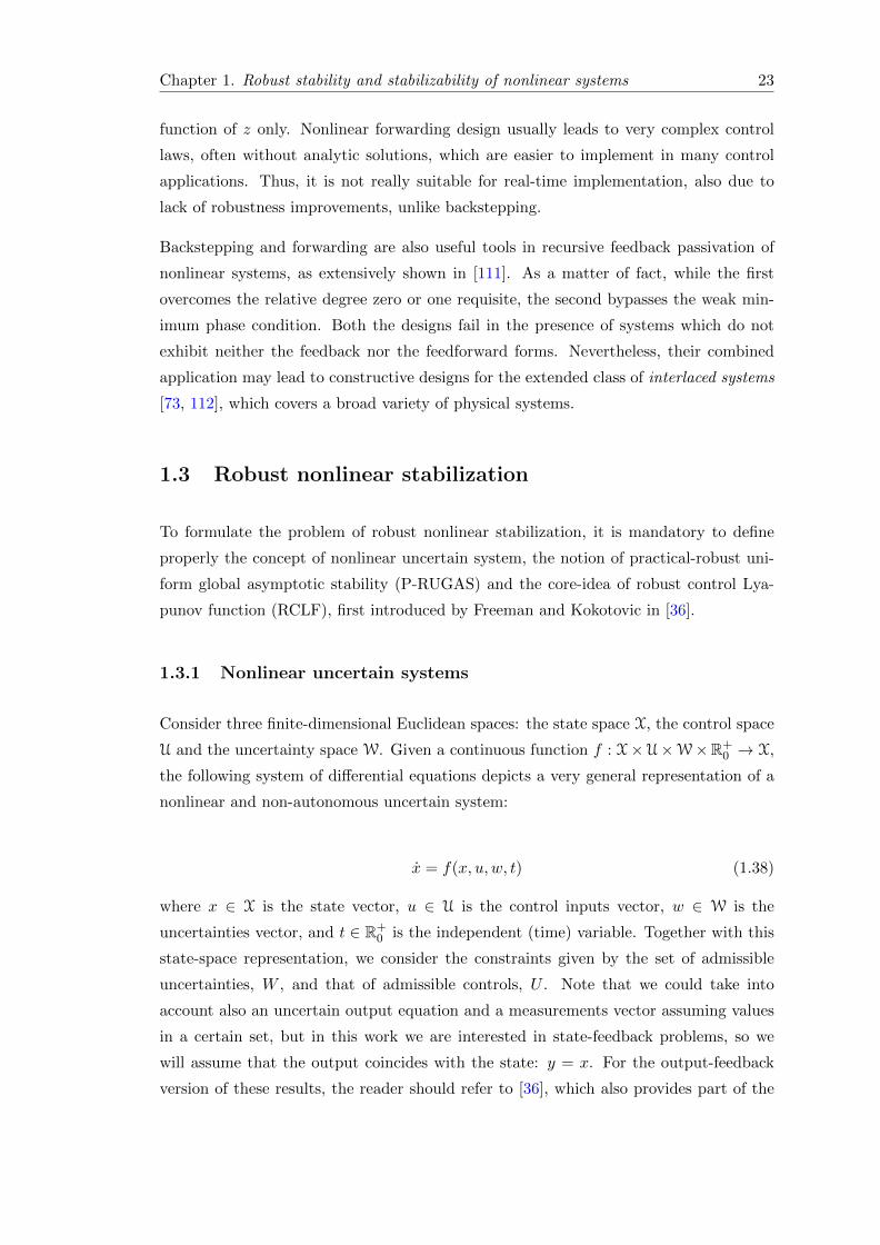
Chapter 1. Robust stability and stabilizability of nonlinear systems 23
function of z only. Nonlinear forwarding design usually leads to very complex control
laws, often without analytic solutions, which are easier to implement in many control
applications. Thus, it is not really suitable for real-time implementation, also due to
lack of robustness improvements, unlike backstepping.
Backstepping and forwarding are also useful tools in recursive feedback passivation of
nonlinear systems, as extensively shown in [111]. As a matter of fact, while the first
overcomes the relative degree zero or one requisite, the second bypasses the weak min-
imum phase condition. Both the designs fail in the presence of systems which do not
exhibit neither the feedback nor the feedforward forms. Nevertheless, their combined
application may lead to constructive designs for the extended class of interlaced systems
[73, 112], which covers a broad variety of physical systems.
1.3 Robust nonlinear stabilization
To formulate the problem of robust nonlinear stabilization, it is mandatory to define
properly the concept of nonlinear uncertain system, the notion of practical-robust uni-
form global asymptotic stability (P-RUGAS) and the core-idea of robust control Lya-
punov function (RCLF), first introduced by Freeman and Kokotovic in [36].
1.3.1 Nonlinear uncertain systems
Consider three finite-dimensional Euclidean spaces: the state space X, the control space
U and the uncertainty space W. Given a continuous function f : X×U×W×R+0 → X,
the following system of differential equations depicts a very general representation of a
nonlinear and non-autonomous uncertain system:
x = f(x, u, w, t) (1.38)
where x ∈ X is the state vector, u ∈ U is the control inputs vector, w ∈ W is the
uncertainties vector, and t ∈ R+0 is the independent (time) variable. Together with this
state-space representation, we consider the constraints given by the set of admissible
uncertainties, W , and that of admissible controls, U . Note that we could take into
account also an uncertain output equation and a measurements vector assuming values
in a certain set, but in this work we are interested in state-feedback problems, so we
will assume that the output coincides with the state: y = x. For the output-feedback
version of these results, the reader should refer to [36], which also provides part of the

Chapter 1. Robust stability and stabilizability of nonlinear systems 24
contents of this section. Let us characterize with precision the spaces above defined in
terms of their set-valued constraints.
We define uncertainty for (1.38) a function w : X × U × R+0 → W such that w(·, ·, t) is
continuous for each fixed t ∈ R+0 and w(x, u, ·) is locally L∞ for each fixed (x, u) ∈ X×U.
Given an uncertainty constraint W : X×U×R+0 W, we define an uncertainty w(x, u, t)
admissible when w(x, u, t) ∈ W (x, u, t) for all (x, u, t) ∈ X× U× R+0 . This kind of rep-
resentation covers a broad class of admissible static uncertainties, including exogenous
and feedback disturbances and other plant and input perturbations. Moreover, this de-
scription is at the foundations of the guaranteed stability framework for robust nonlinear
control [21, 41, 70].
A control for (1.38) is a function u : X×R+0 → U such that u(·, t) is continuous for each
fixed t ∈ R+0 and u(x, ·) is locally L∞ for each fixed x ∈ X. Given a control constraint
U : X × R+0 U, we define a control u(x, t) admissible when u(x, t) ∈ U(x, t) for all
(x, t) ∈ X× R+0 and it is jointly continuous in (x, t).
The vector-field f , together with the two set-valued constraints U and W , constitute the
uncertain nonlinear dynamical system Σ = (f, U,W ). With the expression “solution”
to Σ we mean a solution x(t) to the initial value problem:
x = f(x, u(x, t), w(x, u(x, t), t), t), x(t0) = x0 (1.39)
given an uncertainty vector w(x, u, t), a control u(x, t) and an initial condition (x0, t0) ∈X × R+
0 . The regularity assumptions guarantee that the right-hand side of (1.39) is
continuous in x and locally L∞ in t, and it follows from classical existence theorems
that solutions of Σ always exist, at least locally in t, but need not be unique. Figure 1.1
shows the signal flow diagram of the system.
The system Σ = (f, U,W ) is time-invariant, or autonomous, when the mappings f , U
and W do not explicitly depend on time t. In this case, with slight abuse of notation,
we write f(x, u, w), U(x) and W (x, u). In the same way, we say that a control is time-
invariant when u(x, t) = u(x). Although we have included only static uncertainties and
controls in our formulation, we can accommodate fixed-order dynamics by redefining Σ
according to what is done in [36].
1.3.2 Practical-robust stability and stabilizability
Recall that in Section 1.1.1 we have introduced the notion of PUGAS for a nonlinear
non-autonomous parametrized system. We want to re-define and extend the notion to

Chapter 1. Robust stability and stabilizability of nonlinear systems 25
u ∈ U(x, t)
dx/dt = f(x, u, w, t)
u x
w
K
w ∈ W(x, u, t) u
x
G
Δ
Figure 1.1: Nonlinear robust control paradigm.
the context of nonlinear uncertain systems with control input. With this in mind, we
examine the behavior of the set of solutions of Σ or, which is the same, of (1.38), for all
initial conditions and admissible uncertainties and try to determine which stabilization
property can be achieved with a suitable choice of the robust nonlinear control law u(x).
When every solution of (1.38) converges to a compact residual set Ω ⊂ X containing
a desired operating point (for convenience, the origin 0 ∈ X), we will say that these
solutions (or, equivalently, Ω) are robustly (uniformly globally asymptotically) stable
according to the following definition.
Definition 1.3.2.1 (RUGAS-Ω). Given a control law and a compact set Ω ⊂ X , containing
the origin, the solutions of the nonlinear uncertain system Σ are robustly uniformly globally
asymptotically stable with respect to Ω (RUGAS-Ω) when there exists a class KL function β
such that for all admissible uncertainties and initial conditions (x0, t0) ∈ X × R+0 , all solutions
x(t) exist for all t ≥ t0 and satisfy
|x(t)|Ω ≤ β(|x0|Ω, t− t0) (1.40)
for all t ≥ t0. Moreover, the solutions of Σ are RUGAS when they are RGUAS-0. ♦
Chapter 1. Robust stability and stabilizability of nonlinear systems 26
Note that the RUGAS-Ω implies that the residual set Ω is (robustly) positively invari-
ant. In particular, RUGAS (the particular case with Ω = 0) implies that the origin is
a equilibrium point (in forward time) for every admissible uncertainty and initial con-
dition, which is clearly not necessary using the relaxed RUGAS-Ω property. The robust
stabilization problem for an uncertain nonlinear system Σ which emerges from Definition
(1.3.2.1) is to construct an admissible control law such that the solutions of (1.38) are
RUGAS-Ω for some residual set Ω. In particular, we seek for a practical version of such
property, since we would like to reduce the dimension of Ω at will exploiting control
design parameters. With this in mind, and without loss of generality, let us consider the
extended system Σµ = (f, U,W,M), containing the set M ⊂ Rm of admissible tuning
control parameters. The corresponding state-space representation is then
x = f(x, u(µ), w, t) (1.41)
with µ ∈ M vector of admissible design parameters. It is therefore possible to extend
Definition (1.3.2.1) in the following fashion.
Definition 1.3.2.2 (P-RUGAS). Let M ⊂ Rm be a set of tuning parameters. The uncertain
system (1.41) is said to be practically-robustly uniformly globally asymptotically stable on M
if, given any %(Ω) > 0, with B%(Ω) biggest ball contained in the desired convergence set Ω,
there exists an allowable vector of tuning parameters µp(%(Ω)) ∈ M such that the solutions of
x = f(x, u(µp(%(Ω))), w, t) are robustly uniformly globally asymptotically stable with respect to
B%(Ω) (RUGAS-B%(Ω)). ♦
According to how small we can make the set of convergence of the solutions by a suitable
choice of the control law tuning parameters, we define three types of robust stabilizability
as follows.
Definition 1.3.2.3 (Robust stabilizability). The system Σ is robustly uniformly glob-
ally asymptotically stabilizable when there exists an admissible control and a compact set
Ω ⊂ X , containing the origin, such that the solutions to Σ are RUGAS-Ω. This means that
the distance between the trajectories and the origin of the state space depends strictly on the
dimension of Ω, and cannot made arbitrarily small. When Ω collapse to the origin, the sys-
tem stabilizability property is the simple RUGAS. The system Σµ is practically-robustly
uniformly globally asymptotically stabilizable when for every %(Ω) > 0 there exists an
admissible control and a compact set Ω ⊂ X, satisfying 0 ∈ B%(Ω) ⊂ Ω, such that the solutions

Chapter 1. Robust stability and stabilizability of nonlinear systems 27
to Σµ are RUGAS-B%(Ω). This means that the distance between the trajectories and the origin
of the state space can be made arbitrarily small by an opportune choice of the control design
parameters µ. ♦
Clearly RUGAS with respect to the origin implies practical robust (uniform global
asymptotic) stabilizability, which in turn implies robust (uniform global asymptotic)
stabilizability with respect to a fixed (irreducible in dimension) set Ω.
1.3.3 Robust Control Lyapunov Function
The existence of a Lyapunov function is the most significant necessary and sufficient
condition for the stability of a nonlinear system. The sufficiency was proved by Lyapunov
[76], and the necessity was established half a century later with the advent of the so-
called converse theorems [67]. Since Lyapunov theory deals with dynamical systems
without inputs, it has traditionally been applied only to closed-loop control systems,
that is, systems for which the input has been replaced by a state-feedback control law.
Starting from the early Sixties, some authors began exploiting Lyapunov functions for
feedback design by “making the Lyapunov derivative negative” with proper choice of the
control law [58, 82]. Such ideas have been progressively activated with the introduction
of the concept of control Lyapunov function, of which we have generously discussed in
Section 1.2. This idea can be extended to the class of uncertain nonlinear systems,
introduced in the previous sections, by defining the robust control Lyapunov function,
whose existence, as we are going to show, is a necessary and sufficient condition for
robust nonlinear stabilizability. Most of the contents of this section are rearranged from
[36].
Recall from Section 1.3.1 that an uncertain nonlinear system Σ consists of the triple
(f, U,W ) with continuous generating function f and sets of admissible controls U and
disturbances W . Denote by V(X) the set of all C1 functions V : X×R+0 → R+
0 satisfying,
for all (x, t) ∈ X× R+0 , the inequality
α(‖x‖) ≤ V (x, t) ≤ α(‖x‖) (1.42)
with α and α K∞ functions. The set V(X) is the set of all candidate Lyapunov functions
for testing the robust stability of a nonlinear uncertain system Σ. This set V(X) is
contained in the broader set P(X) of functions which need not to be differentiable or
radially unbounded, that is, the set of all continuous functions α : X × R+0 → R+
0 such

Chapter 1. Robust stability and stabilizability of nonlinear systems 28
that there exist χ1, χ2 ∈ K satisfying χ1(‖x‖) ≤ α(x, t) ≤ χ2(‖x‖) for all (x, t) ∈ X×R+0 .
Given V ∈ V(X) and an uncertain nonlinear system Σ, namely x = f(x, u, w, t), we define
the Lyapunov derivative along the motion LfV : X×U×W×R+0 → R by the equation
LfV (x, u, w, t) :=∂V
∂t(x, t) +
∂V
∂x(x, t)f(x,w, u, t) (1.43)
Clearly LfV is continuous, and it follows from (1.42) that LfV (0, ·, ·, ·) ≡ 0. Now we
are ready to give the definition of robust control Lyapunov function.
Definition 1.3.3.1 (Robust control Lyapunov function). A function V ∈ V(X) is called
a robust control Lyapunov function (RCLF) for an uncertain nonlinear system Σ if there exists
cv ∈ R+0 and αv ∈ P(X) such that
infu∈U(x,t)
supw∈W (x,u,t)
(LfV (x, u, w, t) + αv(x, t)) < 0 (1.44)
for all t ∈ R+0 and all c > cv. ♦
The RCLF extends the CLF in different directions. First, the definition takes into
account not only the control variable, but also the uncertainties, disturbances or generic
perturbations. Second, this notion can be easily extended to measurement feedback as
well. Last, but not least, the parameter cv potentially encompasses all three types of
stabilizability introduced in section 1.3.2, not just asymptotic stabilizability.
This definition particularizes to the special case of autonomous (or time-invariant) sys-
tems in the following fashion.
Definition 1.3.3.2 (Time-inviariant RCLF). A time invariant function V ∈ V(X) is called
a robust control Lyapunov function for an autonomous uncertain nonlinear system Σ if and only
if there exist cv ∈ R+0 and a time invariant function αv ∈ P(X) such that
infu∈U(x)
supw∈W (x,u)
(LfV (x, u, w) + αv(x)) < 0 (1.45)
whenever V (x) > cv. ♦

Chapter 1. Robust stability and stabilizability of nonlinear systems 29
The inequality (1.45) can be interpreted as follows: for every fixed x there exists an
admissible value u for the control such that the Lyapunov derivative is negative for any
admissible value w of the uncertainty. This is a natural generalization of the control
Lyapunov function concept for systems with disturbance inputs.
Example 1.3.3.3 (feedback linearizable systems). Consider a feedback linearizable
system (g1(ξ) nonsingular for all ξ) perturbed by a disturbance input w
ξ = Hξ + L (g0(ξ, w) + g1(ξ)u) (1.46)
Suppose that there is no control constraint, i.e. U(x) ≡ U, and suppose that the
disturbance constraint is such that W (x,U) is bounded for every x ∈ X. Let P be the
symmetric, positive definite, solution to the matrix Riccati equation
HTP + PH − PLLTP + I = 0 (1.47)
The function V (x) = ΦT (x)PΦ(x) = ξTPξ with the selection αv(x) = 12ξT ξ is such that
infu∈U
supw∈W (x,u)
(LfV (x, u, w) + αv(x))
= infu∈U
supw∈W (x,u)
[ξT (HTP + PH)ξ + 2ξTPL (g0(ξ, w) + g1(ξ)u) +
1
2ξT ξ
]= inf
u∈Usup
w∈W (x,u)
[−1
2ξT ξ + ξTPL
(LTPξ + 2g0(ξ, w) + 2g1(ξ)u
)]
=
−12ξT ξ when ξTPL = 0
−∞ when ξTPL 6= 0
(1.48)
Thus we deduce from Definition 1.45 that V is RCLF for system (1.46) with cv = 0. With
this example, we would like to stress that V is also a CLF for the unperturbed version of
system (1.46), the one with w = 0. However, note that not every CLF become a RCLF
when uncertainties perturb a “nominal” dynamics. Generally speaking, this happens
only when the source of uncertainty is matched with the control input, i.e. when the
disturbance w enters the system through the same channel as the control u. Another
way to say this is that the disturbance is in the span of the control action. We will
return later on this point, crucial for robust stabilizability. ♦
1.3.3.1 RCLF in absence of disturbance input
The RCLF is a concept more general than that of CLF, since it takes into account
uncertainties, measurement feedback and non-constant control constraints. We are in-
terested in determining whether or not the RCLF and the CLF coincide. We consider

Chapter 1. Robust stability and stabilizability of nonlinear systems 30
an autonomous system Σ with perfect state measurement, constant control constraint
(U(x) ≡ U), and no uncertainties or disturbance inputs. Recall that a CLF V ∈ V(X)
for x = f(x, u) satisfies
x 6= 0⇒ infu∈U
LfV (x, u) < 0 (1.49)
Clearly, every RCLF for Σ is also a CLF: we want to find out whether or not every CLF
is also a RCLF in this restricted case.
Suppose V is a CLF with the additional property that the left-hand side of the inequality
is bounded away from zero for large x, i.e. for all c > 0 there exists δ > 0 such that
V (x) ≥ c⇒ infu∈U
LfV (x, u) ≤ −δ (1.50)
Every CLF with this additional property is a RCLF according to the definition. As a
matter of fact, if (1.50) is true, then we can find a time-invariant function αv ∈ P(X)
such that adding αv(x) to the left-hand side of (1.49) preserves the inequality. On the
other hand, if a given CLF does not satisfy such extra property, it is not a RCLF because
a suitable function αv does not exist. However, given a CLF not satisfying (1.50), it is
always possible to construct another CLF V satisfying it, and being therefore a RCLF,
see [36] fore more details.
1.3.3.2 RCLF implies robust stabilizability
In [36] several assumptions under which the existence of a robust control Lyapunov func-
tion for a system Σ implies its robust stabilizability, according to Definition 1.3.2.3, are
investigated. There are constraints to be imposed on control and uncertainty spaces U
and W , in terms of lower/upper semi-continuity and, in general, regularity. Another set
of conditions to be fulfilled concerns the structure of the vector field f , which determines
the dynamics of the system Σ, and the structure of W . The first must be a map affine in
the control input, while the second should be independent of u, i.e. W (x, u, t) = W (x, t).
This second set of assumptions could be relaxed when the map f is jointly affine in u
and w: the condition on W changes in that it can be dependent on u, in particular it
must be convex in u. Thus we can state the following sufficiency theorem, whose proof
is detailed in [36].
Theorem 1.3.3.4 (RCLF ⇒ robust stabilizability). Suppose a nonlinear uncertain sys-
tem Σ satisfies some regularity assumptions on U and W , detailed in [36], plus the structural
conditions on f and W . If there exists a RCLF for Σ, then Σ is robustly stabilizable. If,
furthermore, cv = 0, then Σ is practically-robustly stabilizable. Moreover, if Σ and V are

Chapter 1. Robust stability and stabilizability of nonlinear systems 31
time-invariant, then the robustly stabilizing admissible control can always be chosen to be time-
invariant. ♦
1.3.3.3 Small control property
Finally, defining a suitable small control property for nonlinear uncertain systems like
Σ, it is possible to relate the existence of a robust control Lyapunov function to the
robust asymptotic stabilizability of the system considered. Fore more details about the
extension of such a property to the framework of nonlinear uncertain systems, the reader
is again referred to [36]. Substantially, the existence of a robust control Lyapunov func-
tion V which satisfies the small control property, together with all the other conditions
briefly presented above, implies robust asymptotic stabilizability of Σ. Also, if Σ and V
are time-invariant, then the robustly stabilizing admissible control can always be chosen
to be time-invariant.
1.3.3.4 Robust stabilizability implies RCLF
The necessity theorem about robust control Lyapunov functions applies to systems of
the form
x = F (x, d) (1.51)
where F is locally Lipschitz and d(t) is an L∞ exogenous input assuming values in a
nonempty compact convex subset D of a finite-dimensional Euclidean space. First, we
state the following converse theorem.
Theorem 1.3.3.5. Suppose there exists a class KL function β such that, for every initial con-
dition (x0, t0) ∈ X×R and every L∞ exogenous input d(t) taking values in D, the solution x(t)
of (1.51) exists for all t ≥ t0 and satisfies ‖x(t)‖ ≤ β(‖x0‖ , t − t0) for all t ≥ t0. Then, there
exist time-invariant functions V ∈ V(X) and αv ∈ P(X) such that
supd∈D
(LFV (x, d) + αv(x)) ≤ 0 (1.52)
for all x ∈ X. ♦

Chapter 1. Robust stability and stabilizability of nonlinear systems 32
This converse theorem is useful in showing that, at least in the locally Lipschitz case,
the existence of a RCLF is necessary for robust stabilizability. At the same time, we
present the result for robust asymptotic stabilizability, showing the necessity of the small
control property. Again, for the proof the reader is referred to [36].
Theorem 1.3.3.6 (Robust stabilizability ⇒ RCLF). Let Σ be a time-invariant uncer-
tain nonlinear system with generating function f locally Lipschitz. Let the disturbance admis-
sible space W be locally Lipschitz too, with nonempty compact convex values. If Σ is robustly
asymptotically stabilizable via locally Lipschitz time-invariant state-feedback, then there exists a
time-invariant RCLF for Σ satisfying the small control property. ♦

Chapter 2
Structure of an uncertain
nonlinear system
Robust nonlinear control, as already stated, takes into account stabilization problems
of systems whose dynamics is not completely known. A really important role in this
framework is played by the representation used for the uncertain parts of the dynamics,
more briefly the uncertainty. In this section, we define with more details what does the
term “uncertainty” means in the present setting and how uncertainties can be classified.
The most important assumption needed in this context is the possibility to define a
deterministic model of the uncertainty, exploiting it in the subsequent robust nonlinear
design. In particular, only the knowledge of the bounds of these models will be required
to obtain the desired control law. Moreover, we refine the representation of nonlinear
uncertain system and illustrate some of its structural properties. We specialize the class
of systems considered into that of input-affine nonlinear uncertain systems and we give
examples of unstabilizable uncertain systems, highlighting the most common sources of
instability which uncertainty can bring. Next, we introduce the fundamental notion of
matching conditions together with the corresponding relaxed version, that of generalized
matching conditions. Both these conditions set some constraints on system structure
which are strictly related to robust stabilizability. In the final part of the chapter,
we propose a deterministic model of the uncertain terms exploiting the concepts of ∆-
operator and deviation function. As a result, we establish some rules to evaluate the
complex uncertain terms and a novel systematic method to propagate them into system
dynamics.
33

Chapter 2. Structure of an uncertain nonlinear system 34
2.1 Uncertainty representation
Uncertainty represents a part of a physical system that cannot be easily modeled or
precisely known. This means that the model of the system is only partially known. In
the sequel, we will assume that system dynamics can be divided in a nominal, perfectly
known, part and in an uncertain, only partially known, part. Uncertainty is not com-
pletely unknown, because the designer can count on the information about its bounds,
assumed to be known. Note that the use of a partially known model to describe a physi-
cal system not only reflects the reality, but also makes it possible for us to study the way
of designing controls that compensate for the unknowns and achieve better performance
in modern sophisticated systems, like those in the aerospace domain. Recall that the
approach described in this work is totally deterministic, and so are the models and the
uncertainties considered.
Typical uncertainties in deterministic models of physical systems include, but are not
limited to, constant or time-varying parameters of the system, unmodeled dynamics,
modeling errors, unknown inputs such as disturbances, measurement noise, environmen-
tal perturbations of various nature, sampling, quantization noise, etc. In this work we
are going to describe uncertainties as a “lumped”, thus extremely synthetic and practi-
cal, description of all the phenomena that are not depicted in the nominal system model.
Below, we follow in part the classification made by Z. Qu in [106].
There are different ways of classifying the uncertainties, for instance according to:
• functional dependence and structure;
• relationship to the control input;
• size of the bounding functions;
• continuity and other regularity assumptions;
• location in system equations.
A first notable distinction to make is between dynamic (with memory) uncertainties and
static (memoryless) uncertainties.
1. Dynamic uncertainties, also called unmodeled dynamics, are quite difficult to
consider in control design, so they are usually neglected due to their high-frequency
response. Sometimes, their effect on system dynamics is studied using approxima-
tions or asymptotic methods like singular perturbations, center manifold theory
or more practical time-scales separation arguments. If neglected, these uncertain

Chapter 2. Structure of an uncertain nonlinear system 35
terms may lead to instability of the closed-loop system. They are due to a lack of
dynamic description of the model used for control design, often highly simplified
to make the design phase easier. A remarkable example of unmodeled dynamics
is the high-frequency actuator dynamics of an air-to-air missile, one of the case-
studies analyzed in the following. Also the equations of the flexible modes in a
spacecraft with appendages can be considered unmodeled dynamics.
2. Static uncertainties can be taken into account more easily in control design,
nonetheless they still represent a danger for stability. Usually, they are para-
metric uncertainties, modeling errors or disturbances. Typical examples of static
uncertainties, that may be time-varying, state, and control dependent, are the
aerodynamic forces and moments in the missile equations of motion. Another no-
table example is the parametric uncertainty in the inertia moments of a flexible
spacecraft, as in one of the application studies made in this work.
Another very important distinction emerges between unstructured and structured un-
certainties.
1. Unstructured uncertainties are those that are bounded by a function of the
state and time in some norm and can assume any arbitrary value or function within
the size of the given bounding function. There is no additional information upon
the uncertainty structure, only that of its bounding function.
2. Structured uncertainties are those for which some information in addition to
their bounding functions is available. This information is related to the functional
structure of the uncertainty itself.
Consider a deterministic time-domain uncertainty ∆(x, t), for instance a scalar function,
such that:
|∆(x, t)| ≤ ‖x‖ (2.1)
where x ∈ Rn. Without any information about ∆(x, t) other than its bounding function
‖x‖, the uncertainty is said to be unstructured. This particular uncertainty ∆(x, t) is
also called sector-bounded as its bounding function is linear with respect to the norm
of the state. Uncertainty ∆(x, t) is said to be structured if its functional dependence
on the state and time can be described to some extent. The most common type of
structured uncertainties is the class of so-called parametrizable uncertainties, that is,
uncertainties that can be characterized through a certain, more or less defined, func-
tional expression. If the function is known except for a finite number of unknown,
possibly time-varying, parameters, the uncertainty is called linearly parametrizable. An

Chapter 2. Structure of an uncertain nonlinear system 36
example of linearly parametrizable uncertainty is ∆(x, t) = aT (t)x, where a(t), with
‖a(t)‖ ≤ 1, is a vector of unknown time-varying or constant parameters. If otherwise,
for instance, ∆(x, t) = bT (x, t)x where ‖b(x, t)‖ ≤ 1, the uncertainty is said to be non-
linearly parametrizable. It should be noted that several levels of information may be
obtained for uncertainties, particularly for structured ones. As an example, consider
again the structured uncertainty ∆(x, t) = bT (x, t)x with ‖b(x, t)‖ ≤ 1. Once the non-
linear parametrization is given, we can continue to specify if the uncertain vector b(x, t)
is structured. For vector uncertainty b(x, t) to be structured, the expressions of its
uncertain elements are important. If
b(x, t) = c(x, t)x
1 + ‖x‖2(2.2)
with ‖c(x, t)‖ ≤ 2, the same question of being structured or not can be raised again
for the vector c(x, t). This process of exploring uncertainty information stops when
all physical understandings of the system are exhausted. At the end the uncertainties
should be either unstructured or linearly parametrized.
Given a bounding function, the unstructured uncertainties entailed by it constitute a set
of infinite elements. Obviously, structured uncertainties are special, deterministic, real-
izations of unstructured uncertainties bounded by the same bounding function. Hence,
treating structured uncertainty as unstructured inevitably enlarges the set of admissible
elements and in turn makes analysis and control design conservative. It will be shown
in some examples that the location of the uncertainties in system dynamics and their
nature may determine whether the uncertain system is stabilizable, and that exploiting
such structural information is a crucial point in control synthesis. Nevertheless, available
analysis techniques and control design procedures are not capable of taking into account
every piece of information known about uncertainties. As a result, uncertainties being
unstructured at a certain level are often much easier to be handled in analysis and con-
trol design than structured uncertainties. It is in these cases that a conservative result
may have to be concluded. There is clearly a compromise to deal with concerning the
complexity of the design and its conservatism.
Once defined in an accurate way the concept of uncertainty, we are now ready to present
the general problem of robust nonlinear control.
Definition 2.1.0.7 (Robust nonlinear control problem). The problem of controlling non-
linear uncertain systems, also referred to as the robust nonlinear control problem, is to
design a fixed (i.e. uncertainty independent) controller which guarantees design requirements in
Chapter 2. Structure of an uncertain nonlinear system 37
the presence of significant uncertainties bounded in size by either some constant or some well-
defined functions of the state and time. If it exists, such a stabilizing control is called robust
nonlinear control, and must be suited to achieve stability and a desired level of performance
for the closed-loop system. ♦
The adjective “robust” is used to reflect the fact that the specific property holds for all
possible uncertainties within their bounds (or bounding functions). The other two key
phrases in the above definition are “significant” and “bounded in size”. Insignificant
uncertainties need not be considered since all stable feedback control systems possess a
certain level of robustness against small perturbations. Moreover, the boundedness of
uncertainties is a compulsory requirement for the success of nonlinear robust control syn-
thesis. Note that, however, robust nonlinear control laws can be designed merely know-
ing the existence of some bounds or bounding functions of the uncertainties, without
requiring the knowledge of the bounds amplitude itself, but with compulsory limitations
on the performance of the control system. This happens to be the case, for instance, of
the famous redesign technique called nonlinear damping presented in [62]. Therefore,
the superiority of robust control and its difference from other design methodologies are
due to the fact that uncertainties are only required to be bounded. In fact, in compar-
ison, classical adaptive control and learning control can be used to handle only those
systems with linearly parametrized uncertainties. For systems with both unstructured
and parametrizable uncertainties, a combination of robust and adaptive control can have
success.
Basically, the design phase of robust nonlinear control consists of three steps:
• Study the nominal system (in which system uncertainties are assumed to be zero)
and design a stabilizing nominal control.
• Find a Lyapunov function for the uncertain system.
• Develop a robust controller through a Lyapunov argument in which enlargement
and size domination will be employed.
Robust control design is usually based on a nominal control design for the nominal
system, since the presence of uncertainties complicates the synthesis and because robust
control reduces to the nominal as the size of uncertainties becomes zero. There are
two additional reasons why a nominal design is required. First, stability analysis of
uncertain systems is always done with respect to the equilibrium point of the nominal

Chapter 2. Structure of an uncertain nonlinear system 38
system. Second, the Lyapunov function for the uncertain system, at least in solving the
easiest problems, can be chosen to be that of the nominal system. Nominal control design
and robust control design may be combined together to achieve stabilization. In some
cases, it is easier to neglect some known dynamics to develop a simpler nominal control
and treat them as uncertainties to handle in the following robust control synthesis. The
enlargement process consists in exploiting the knowledge of the bounds to develop the
Lyapunov derivative inequality, enlarging the uncertainties to their known maximum
possible sizes. This implies that a robust nonlinear control design is, in essence, a
worst-case design. Size domination, finally, means that the control law developed makes
the Lyapunov derivative satisfy the dissipation inequality by dominating in size all the
uncertain terms in it. For further conceptual considerations about the philosophy of
nonlinear robust control, the reader could refer to [106].
2.2 Input-affine nonlinear uncertain systems
The generic state-space representation of a nonautonomous uncertain nonlinear system
was already given as (1.38). However, it is very difficult to develop a robust nonlinear
controller for a system with such a highly-nonlinear structure. Therefore, we are going
to take into account for the rest of the work the input-affine version of (1.38), because
the control techniques that we will present need this structure to be properly applied.
More in detail, we consider systems of the form
x = a(x,w, t) +B(x,w, t)u (2.3a)
:= f(x, t) + ∆f(x,w, t) +G(x, t)u+ ∆G(x,w, t)u (2.3b)
where x ∈ X ⊂ Rn is the state vector, u ∈ U ⊂ Rp is the control inputs vector, t ∈ R+0 is
the time, and w ∈ W ⊂ Rs is the vector of time-varying uncertain variables. In (2.3a),
w is simply a lumped description of all the uncertainty of the system. The second
representation (2.3b) is a structured version of (2.3a). As a matter of fact, f and G
are the known, nominal, parts of a and B respectively, while ∆f and ∆G represent
their uncertain components. Thus, the representation (2.3b) emphasizes a structural
separation between the nominal dynamics and the uncertain one.
To guarantee existence and uniqueness of the solutions of (2.3), some regularity assump-
tions on system equations are needed. A naıf assumption could be restricting the vector
field a+Bu to be sufficiently smooth. However, this could be too restrictive and could
cause a lack in the representation power of (2.3). As a consequence, we employ the
following two assumptions [106], which are indeed less restrictive.

Chapter 2. Structure of an uncertain nonlinear system 39
Assumption 2.2.0.8. In the nonlinear uncertain system (2.3), the vector field a+Bu
is Caratheodory, and the uncertain vector w is Lebesgue measurable. ♦
Assumption 2.2.0.9. In the nonlinear uncertain system (2.3), the vector field a+Bu
is locally uniformly bounded. ♦
If we make the extra assumption of a state-dependent, time-varying, vector of uncer-
tainties w(x, t), we can further simplify (2.3a) and (2.3b) into:
x = f(x, t) + ∆f(x, t) +G(x, t)u+ ∆G(x, t)u (2.4)
which is the representation used throughout the rest of the work to construct a robust
nonlinear controller.
2.2.1 Examples of unstabilizable uncertain systems
Although it would be ideal if robust control could be designed to stabilize all uncertain
systems in the fully nonlinear form (1.38), the following examples show that this is too
hard to even conceive, since not all the uncertain systems are stabilizable [106].
Example 2.2.1.1 (Structural change). Consider the second-order system:
x1 = x2 + ∆(x1, x2)
x2 = u(2.5)
in which the uncertainty ∆(·, ·) is bounded as follows
|∆(x1, x2)| ≤ 2 + x21 + x2
2 (2.6)
One can easily see that the system is not stabilizable since one possibility of additive
uncertainty within the given bounding function is −x2 + x1. Physically, the system
becomes unstabilizable since uncertainty can change its structure in a critical manner.
Note that, as a matter of fact, part of system dynamics becomes unstable and, also,
decoupled from the rest of the system and from the control input. As will be shown
later, such an uncertainty causing the loss of controllability belongs to the class of so-
called unmatched uncertainties. ♦
Example 2.2.1.2 (Unknown control direction). Consider the scalar system
x = x+ (1 + ∆(x))u (2.7)

Chapter 2. Structure of an uncertain nonlinear system 40
where uncertainty is bounded as |∆(x)| ≤ C for some C ≥ 1. The system is not
stabilizable since ∆(x) could be −1, and so the system is not subject to any control and
is simply unstable. The uncertain term may also be such that the whole sum 1+∆(x) is
uncertain because of C > 1, and therefore any control introduced may have an adverse
effect on stability, since it may cause the state to grow out of bound more quickly. In
these cases, keeping the control input at zero is the best choice, and the system would
be unstabilizable if any control is needed. ♦
Example 2.2.1.3 (Unidirectional control). Consider the scalar system
x = ∆(x)x+ u2 (2.8)
where uncertainty is bounded as 0 < ∆(x) ≤ 1. The system is not stabilizable since, no
matter what choice is made for u, the control action in x is always unidirectional (pos-
itive). In fact, any scalar uncertain system is not stabilizable if the designer cannot make
x be both positive and negative upon his choice through selecting in appropriate way u
(specifically, through choosing robust control to dominate all possible uncertainties). ♦
Although the dynamics of the above examples are quite simple, they furnish intuitive
explanations of what may lead uncertain systems to be unstabilizable. In particular, we
may distinguish two categories of issues:
1. Loss of controllability, due to either the combination of a broken input-output
chain and unstable dynamics, as in example 2.2.1.1, or the presence of both feed-
back and feedforward paths.
2. Unknown or unidirectional control contribution to the differential equations,
as in examples 2.2.1.2 and 2.2.1.3.
The ultimate objective of robust control theory and design of nonlinear uncertain systems
is twofold.
1. First, if necessary, determine the least requirements, called structural conditions,
on the system (2.3) such that it can be stabilized or, in general, controlled. This
is done in the two sections below.
2. Second, find procedures under which robust control u can be systematically de-
signed. The key issue in the design is the search for robust control Lyapunov func-
tions and their associated robust controllers, which may be different for achieving
different types and levels of performances. This is done in the final sections of this
part of the work.

Chapter 2. Structure of an uncertain nonlinear system 41
2.2.2 Matching conditions
To find a suitable robust control for (2.4), we need to analyze further the structure of the
representation in terms of the uncertainties. The main structural property characterizing
the uncertain terms in (2.4) is the matching condition, under which the dynamics assume
the form:
x = f(x, t) +G(x, t) [u+ ∆(x, u, t)] (2.9)
As before, the vector fields f and G represent the known functions of the nominal system
model, while ∆(x, u, t) is an unknown function which lumps together various structured
and unstructured uncertainties. Note that the uncertainty ∆(x, u, t) enters the system
in the same channel of the control input u. This property is recognized by the fact that
∆(x, u, t) is multiplied by the same matrix function G as the control input.
Let us define more precisely the matching conditions for systems of the form (2.4) as
follows.
Definition 2.2.2.1 (Matching conditions). Consider an input-affine uncertain system of the
form
x = f(x, t) + ∆f(x, t) +G(x, t)u+ ∆G(x, t)u (2.10)
with all the properties of (2.4). The above system is said to satisfy the matching conditions if
the uncertain terms can be factorized as follows:
∆f(x, t) = G(x, t)∆f ′(x, t)
∆G(x, t) = G(x, t)∆G′(x, t)(2.11)
and if there exists a positive constant ε such that
‖∆G′(x, t)‖ ≤ 1− ε (2.12)
The uncertainties satisfying the matching conditions are called matched uncertainties. ♦
According to Definition 2.2.2.1, the matched uncertainties act “along” the distribution
spanned by G(x, t), whereas unmatched uncertainties are off-the-distribution compo-
nents. Roughly speaking, matched uncertainties represent variations of the intensity in
the direction of the control action, while unmatched uncertainties act on directions on
which there is no apparent control authority.

Chapter 2. Structure of an uncertain nonlinear system 42
To illustrate the rationale for the inequality condition (2.12), let us rewrite system (2.4),
assuming satisfied conditions (2.12), as follows
x = f(x, t) +G(x, t)[∆f ′(x, t) + (1 + ∆G′(x, t))u
](2.13)
Recalling some basic notions about necessary conditions for output controllability, we
observe that if the bounds of the uncertain term multiplying the control are allowed to
be greater than unity: ∥∥∆G′(x, t)∥∥ > 1 (2.14)
then the control direction cannot be determined, thus any control input may cause the
system to grow unstable. Furthermore, if the uncertain term multiplying the control
input is such that: ∥∥∆G′(x, t)∥∥ = 1 (2.15)
then a singularity occurs when ∆G′(x, t) = −1. In such a case, with no control authority,
stabilization cannot be achieved.
It can be seen for instance from the above example 2.2.1.2, that if the unknown functions
were replaced by known bounding functions satisfying the matching conditions, then one
could easily choose a control law to cancel their effects and stabilize the system. This
is the basic idea of the robust control design methodology called Lyapunov redesign,
presented later in Section 3.1.
2.2.3 Generalized matching conditions
A step forward in nonlinear robust control design is made by taking into account systems
which do not satisfy the matching conditions, i.e. systems containing the so-called
unmatched uncertainties, which do not enter the system dynamics in the input channel
as the matched ones. For this category of systems, very frequent in applications, recent
investigations of the concept of robust control design have been directed toward the
discovery of robust stabilizing controllers. Important results can be found in [108]. These
results were formulated by considering the idea of a stability margin of the stabilized
nominal system. Qu and Dorsey demonstrated that uncertain systems with arbitrarily
large unmatched uncertainty can be stabilized if the nominal system can be stabilized
with an arbitrarily large convergence rate (i.e. arbitrarily large stability margin). Qu,
in [103], proposed a robust control design for a relaxed set of conditions referred to as
equivalently matched uncertainties (or EMUs). The main concept for the EMU based
design is to take advantage of the non-uniqueness of the Lyapunov function candidates,
and demonstrates a set of conditions on the unmatched uncertainties that allows them
Chapter 2. Structure of an uncertain nonlinear system 43
to be handled in the Lyapunov argument as if they were matched. These results were
still fairly restrictive in scope, and limited in practical applications. After some results
for linear systems, the concept of generalized matching condition (or GMCs) was finally
introduced in an important paper of Qu [104]. In this paper, it was also proposed
a systematic robust control design procedure to guarantee global stability under the
GMCs.
The definition of generalized matching conditions is somewhat very technical and lies
outside the purpose of this work. The only conceptual question is in describing the
general structure of an uncertain nonlinear system which meets the GMCs, as follows:
x1 = f1(x1, t) + ∆f1(x1, w1, t) + g1(x1, x2, w1, t)
. . .
xi = fi(x1, . . . , xi, t) + ∆fi(x1, . . . , xi, wi, t) + gi(x1, . . . , xi+1, wi, t)
. . .
xm = fm(x1, . . . , xm, t) + ∆fm(x1, . . . , xm, wm, t) + gm(x1, . . . , xm, u, wm, t)
(2.16)
where col(x1 . . . xm) is the state vector of the system, which is decomposed into state
sub-vectors xi ∈ Rni , i = 1, . . . ,m. Clearly, one must have
n1 + n2 + . . .+ nm = n (2.17)
with n dimension of the state space. The vector u ∈ Rnm+1 contains the control inputs
of the subsystems. The variables wi = 1, ...,m, represent the uncertain time-varying
parameters, and their domain is a prescribed compact set of Rpi . The conditions that
(2.16) should fulfill to satisfy GMCs are fully presented in [106], to which the reader
should refer for a deeper understanding. The reader should only be acknowledged that
these conditions impose constraints on the dimensions of the subsystems, in a lower
triangular form fashion, on the factorization of the gi vector fields (that should also be
Lipschitz functions) and, of course, on the boundedness of the uncertain terms, namely:
‖∆fi(x1, . . . , xi, wi, t)‖ ≤ ρi(x1, . . . , xi, t), ∀ (x1, . . . , xi, wi, t) (2.18)
Note that ρi are known continuous functions that are uniformly bounded w.r.t. t, and
locally uniformly bounded w.r.t. x.
Moving ahead to a more general structure of system, we should consider the generic
class of uncertain systems which do not satisfy matching conditions, nor the generalized
matching conditions. Qu and Kaloust addressed this problem in [59] and developed a

Chapter 2. Structure of an uncertain nonlinear system 44
generic procedure for robust nonlinear control design of these systems. In the follow-
ing, we will consider separately the problem of stabilization of a system which meets
the matching conditions, using the approach named Lyapunov redesign, and the (more
difficult) one of stabilizing a system satisfying just the generalized matching conditions,
using the so-called robust backstepping approach. The fusion of these two methods re-
sults in a novel approach, which we call recursive Lyapunov redesign, whose aim is the
stabilization of systems with a more general structure, in which the matched uncertain-
ties may be control-dependent.
2.3 Uncertainty modeling
The first step in robust controller design for nonlinear systems is to model the uncertainty
which affects the nominal equations in terms of deviations from the nominal values of
system parameters. In this part of the work, we propose a novel approach to rapidly
evaluate the deterministic model of such uncertainty.
First, we need to assume that system (2.4) may be simplified as follows
x = f(x) + f(t) + ∆f(x, t) +G(x)u+ G(t)u+ ∆G(x, t)u (2.19)
so that we can consider the time-varying terms as part of the uncertain terms, namely
∆f(x, t) = f(t) + ∆f(x, t)
∆G(x, t) = G(t) + ∆G(x, t)(2.20)
Thus, disregarding the · for simplicity of notation, system (2.19) can be written in the
following form:
x = f(x) + ∆f(x, t) + [G(x) + ∆G(x, t)]u. (2.21)
Note that f(x) and G(x) are completely known vector and matrix functions. As a
consequence, we can further define
fact(x, t) = fnom(x) + ∆f(x, t)
Gact(x, t) = Gnom(x) + ∆G(x, t)(2.22)
where clearly fnom(x) = f(x) and Gnom(x) = G(x) are the nominal values of the func-
tions, perfectly known, while with fact and Gact we denote the actual, true, values that
the vector function f and the matrix function G assume at time t. The gap between the
real and the nominal values is embedded into the uncertainty functions ∆f and ∆G,
which are time-varying, deterministic perturbations of the nominal values of system’s

Chapter 2. Structure of an uncertain nonlinear system 45
vector and matrix functions. The first thing to do to define these uncertainty functions
is to define the scalar ∆ operator, which applies point-wisely to the nominal compo-
nents of system’s vectors and matrices giving, one by one, the components of the vector
uncertainty functions.
Definition 2.3.0.1. [∆-operator and deviation function] The ∆-operator, when applied to
the nominal value of a function f depending on uncertain parameters, gives a measure of the
gap between that value and its actual one. The way the ∆ operator perturbs a nominal value
really depends on the design purposes and on modeling necessities. The straightforward choice
we make is that of using what we call deviation function σ(t), such that
∆f = σ(t)fnom (2.23)
where σ(t) has the form
σ(t) = k sin(ωt)ept (2.24)
Its amplitude k represents the amount of uncertainty which perturbs the nominal value of the
function to which σ(t) is applied. We let it be a constant value, but in fact it could be allowed to
depend on time. The frequency ω describes the speed of variation of the actual function’s value
around the nominal one. The constant p, less or equal than zero, defines if the perturbation is
transient or permanent: throughout the study we will put this equal to zero, considering only
persistent uncertainties. ♦
By definition, the ∆-operator acts on known values like the derivative operator acts on
constant values. When a parameter p or a function is considered known, its nominal
value coincides with the actual one, and the ∆ operator gives zero as result, namely:
∆(pnom) = 0 (2.25)
Nevertheless, its real purpose is acting as a perturbation operator when applied to an
unknown parameter. In this simple case it returns the product of the deviation function
with the nominal value of the parameter.
∆(p) = σp(t) · pnom = ∆p (2.26)
When ∆ is applied to a generic function f depending on an uncertain vector of param-
eters p, it takes the general form
∆(f(·, p)) = ∆f (·, pnom, σp1 , . . . , σpN ) (2.27)

Chapter 2. Structure of an uncertain nonlinear system 46
with a different deviation function σpi for each parameter in p.
In the sequel, with in mind our case study, we characterize the structure of ∆f when
applied to functions with polynomial dependence on the uncertain parameters. These
functions depend also on known parameters ai and show an affine dependency on them.
We start by considering the case of a single uncertain parameter z:
f = arzr + ar−1z
r−1 + · · ·+ a1z + a0 (2.28)
The application of the ∆ operator preserves the affinity:
∆(f) = ar∆(zr) + ar−1∆(zr−1) + · · ·+ a1∆(z) (2.29)
In a way similar to the derivative operator, ∆ acts on the polynomial uncertain term zr
in this way:
∆(zr) = ∆(z · z · · · z) = (∆z)r + rzr−1∆z +r(r − 1)
2zr−2(∆z)2
+ . . .+r!
i!(r − i)!zr−i(∆z)i + . . .+ r(∆z)r−1z
(2.30)
that means that it is distributed across the polynomial according to the rule of simple
combinations without repetitions. At each application of ∆ we need to group i dis-
tinct elements into a subset, and the number of these subsets is given by the Newton
coefficient. This procedure is of direct derivation from the Leibniz rule for the differen-
tiation of a product, with the notable difference that multiple ∆-products are allowed,
since we are dealing with finite values and not infinitesimal ones. Keeping in mind that
∆z = ∆(z) = σ(t)z1 and consequently grouping powers of z, we obtain:
∆(zr) = σr(t)zr + rσ(t)zr +r(r − 1)
2σ2(t)zr
+ . . .+r!
i!(r − i)!σi(t)zr + . . .+ rσr−1zr
(2.31)
Or in a more compact form, re-ordering and post-multiplying by zr:
∆(zr) =
(r∑i=1
r!
i!(r − i)!σi(t)
)zr (2.32)
1For simplicity, in the following we omit the subscript nom, since it is clearly the nominal value of theparameter z the one we refer to when applying the deviation function.

Chapter 2. Structure of an uncertain nonlinear system 47
Applying repeatedly the same arguments on every power of z in f we obtain:
∆(f) = ar
(r∑i=1
r!
i!(r − i)!σi(t)
)zr
+ ar−1
(r−1∑i=1
(r − 1)!
i!(r − 1− i)!σi(t)
)zr−1 + . . .+ a1σ(t)z
(2.33)
Since we use simple combinations without repetitions, the whole calculus developed is
valid also for polynomial functions of r different parameters z1, z2, . . . , zr. Thus the
following proposition holds.
Proposition 2.3.0.2. Let fnom be the nominal value of a scalar function depending on known
terms ar, ar−1, . . . , a1, a0 and unknown terms whose nominal values are z1, z2, . . . , zr.
fnom = ar · (z1 · z2 · · · zr) + ar−1 · (z1 · z2 · · · zr−1) + . . .+ a1 · z1 + a0 (2.34)
The application of the ∆ operator with the associated deviation function σ(t) results in:
∆(fnom) = ar
(r∑i=1
r!
i!(r − i)!σi(t)
)fr
+ ar−1
(r−1∑i=1
(r − 1)!
i!(r − 1− i)!σi(t)
)fr−1 + . . .
+ ar−j
(r−j∑i=1
(r − j)!i!(r − j − i)!
σi(t)
)fr−j + . . .+ a1σ(t)f1
(2.35)
where fr = z1 · z2 · · · zr, fr−1 = z1 · z2 · · · zr−1 and so on until f1 = z1. ♦
Proof. The ∆ operator applies to the sets of r parameters z of fr by constituting subsets
using simple combinations without repetitions, more in detail:
• 1-subset the first subset is only one and given by the simultaneous application of
∆ to all the r parameters, i.e. set1 = ∆z1∆z2 · · ·∆zr.
• r-subsets There are two subsets composed by r elements, the first given by the
application of ∆ to the single elements, one-by-one, and the second given by the

Chapter 2. Structure of an uncertain nonlinear system 48
application of ∆ to r − 1 groups of elements, both r times:
first r− subset :
∆z1(z2z3 · · · zr) + ∆z2(z1z3 · · · zr) + . . .+ ∆zr(z1z2 · · · zr−1)
second r− subset :
(∆z1∆z2 · · ·∆zr−1)zr + (∆z1 · · ·∆zr−2∆zr)zr−1
+ . . .+ (∆z2∆z3 · · ·∆zr)z1
(2.36)
• Going on with the analysis, we find other two subsets composed by r(r−1)2 elements
obtained through the application of ∆ to 2 and r − 2 elements at once.
• The iterative perturbation process goes on, using always simple combinations to
form the remaining couples of subsets, each of them formed by the same number
of elements given by the Newton coefficient.
The associative property of the deviation function allow for the simplification, so we
obtain:
∆(fr) = σr(t)(z1z2 · · · zr) + rσ(t)(z1z2 · · · zr)
+r(r − 1)
2σ2(t)(z1z2 · · · zr) + . . .
+r!
i!(r − i)!σi(t)(z1z2 · · · zr) + . . .+ rσr−1(t)(z1z2 · · · zr)
=
(r∑i=1
r!
i!(r − i)!σi(t)
)fr
(2.37)
This procedure clearly still holds for all the other terms of the polynomial, from fr−1 to
f1. The linearity of the ∆ operator then yields (2.35).
In the following, we will need to evaluate the uncertain envelopes of quotients between
uncertain parameters. With this aim, it is possible to establish the following result.
Proposition 2.3.0.3. Let fnom be a function expressed by the quotient of two uncertain param-
eters, whose nominal values are z1 and z2, multiplied by a known value a
fnom = a · z1
z2(2.38)
The application of the ∆ operator results in the following uncertain envelope:
∆fnom = fnomσ1(t)− σ2(t)
1 + σ2(t)(2.39)
where σ1 and σ2 are the deviation functions associated to, respectively, z1 and z2. ♦
Chapter 2. Structure of an uncertain nonlinear system 49
Proof. By definition, we have:
z1 =1
afnomz2 (2.40)
the linearity-in-the-known-terms of ∆ yields:
∆1z1 =1
a(∆fnom∆2z2 + ∆fnomz2 + fnom∆2z2) (2.41)
With ∆i we underline that we are applying to the parameter zi the deviation function
σi(t). Grouping and rearranging equation (2.41) we obtain:
∆fnom =a∆1z1 − fnom∆2z2
∆2z2 + z2(2.42)
Finally, substituting into the right member the expression of fnom in terms of the other
parameters and using the deviation functions σ1 and σ2, we obtain:
∆fnom = az1
z2
σ1(t)− σ2(t)
σ2(t) + 1= fnom
σ1(t)− σ2(t)
σ2(t) + 1(2.43)
which is exactly (2.39), q.e.d.
We are going to massively use these results in missile autopilot design, where the complex
structure of the aerodynamics parameters requires simplified procedures to evaluate the
uncertain envelopes.
Chapter 3
Robust nonlinear control design
In this chapter we establish the main results of the work. We begin by recalling the
Lyapunov redesign technique and introducing a revisited version of it, exploiting suit-
able differentiable sigmoid functions, the robust control functions, in order to avoid the
problem of chattering in the implementation phase. Next, we recall the robust back-
stepping technique, and finally we present our main result, consisting of the fusion of
the two approaches, the technique called recursive Lyapunov redesign. This technique
allows to compensate also control-dependent uncertainties, which are common in certain
nonlinear aerospace dynamics, like tail-controlled missile dynamics. In the last part of
the chapter, we recall the stabilization technique of Immersion & Invariance as a tool
of robustification of nonlinear control laws with respect to higher-order dynamics. We
propose a solution in the case of a particular class of systems in feedback form using one
step of backstepping and a nonlinear domination argument.
3.1 Lyapunov redesign revisited
To handle matched uncertainties it is possible to use a classical technique presented
in [62], the Lyapunov redesign. This method is of sure effectiveness, but leads to a
discontinuous control law. We propose here a revisited version of this method that
yields a C1 (continuous with its first derivative) control law. The procedure applies to
systems which satisfy the matching condition, namely:
x = f(x, t) +G(x, t) [u+ ∆(x, u, t)] (3.1)
where x ∈ Rn and u ∈ Rm. Note that ∆ is an unknown function lumping together various
structured and unstructured uncertainties and satisfying the matching condition, since
50

Chapter 3. Robust nonlinear control design 51
it lies in the span of the control input. Suppose that the nominal system
x = f(x, t) +G(x, t)ψ(x, t)
is stabilized by a known nominal1 feedback control law (for instance, feedback lineariza-
tion or backstepping) u = ψ(x, t). Such state feedback renders the nominal closed-loop
system
x = f(x, t) +G(x, t)ψ(x, t) (3.2)
uniformly globally asymptotically stable (UGAS). Suppose further that we know a Lya-
punov function for (3.2), i.e. a continuously differentiable function V (x, t) that satisfies
the inequalities:
α1(‖x‖) ≤ V (x, t) ≤ α2(‖x‖)∂V
∂t+∂V
∂x[f(x, t) +G(x, t)ψ(x, t)] ≤ α3(‖x‖)
(3.3)
where α1, α2 are class K∞ functions, while α3 is a class K function. Assume that, with
u = ψ(x, t) + v, the uncertain term satisfies the inequality:
‖∆(x, ψ(x, t) + v, t)‖ ≤ ρ(x, t) + k0 ‖v‖ , 0 ≤ k0 < 1 (3.4)
where ρ is a non-negative continuous function. The above inequality defines the bound-
ing function of the uncertain term ∆, and it is the only information we need to know
about it. The bounding function ρ represents a measure of the maximum size the uncer-
tainty may assume: we will not require it to be small, only to be known. We want to find
an expression for v such that, under the overall control u = ψ(x, t) + v, the uncertain
system (3.1) is UGAS. The uncertain closed-loop system under the feedback u is:
x = f(x, t) +G(x, t)ψ(x, t) +G(x, t) [v + ∆(x, ψ(x, t) + v, t)] . (3.5)
We exploit the same Lyapunov function of the nominal system (from this re-use, the
name “re-design”) as a robust control Lyapunov function for the uncertain system. The
derivative along the motion takes the form (omitting for brevity the arguments of the
various functions):
V =∂V
∂t+∂V
∂x(f +Gψ) +
∂V
∂xG (v + ∆) ≤ −α3(‖x‖) +
∂V
∂xG (v + ∆) . (3.6)
1Here and throughout the work we call “nominal” a control law which is designed using only theperfectly known (nominal) parts of the dynamics.

Chapter 3. Robust nonlinear control design 52
Set wT =∂V
∂xG and rewrite the last inequality as:
V ≤ −α3(‖x‖) + wT v + wT∆. (3.7)
Note that, due to the matching conditions, the uncertain term ∆ appears on the right-
hand side exactly at the same point where v appears. Consequently, it is possible to
choose v to cancel the (eventually destabilizing) effect of ∆ on V . Exploiting inequality
(3.4), we obtain:
wT v + wT∆ ≤ wT v + ‖w‖ ‖∆‖ ≤ wT v + ‖w‖ [ρ(x, t) + k0 ‖v‖] . (3.8)
Taking
v = −η(x, t) · w
‖w‖(3.9)
with η non-negative function, we obtain
wT v + wT∆ ≤ −η ‖w‖+ ρ ‖w‖+ k0η ‖w‖ = −η(1− k0) ‖w‖+ ρ ‖w‖ . (3.10)
Choosing then
η(x, t) ≥ ρ(x, t)
1− k0(3.11)
for all (x, t) ∈ Rn × [0,∞) yields
wT v + wT∆ ≤ −ρ ‖w‖+ ρ ‖w‖ = 0. (3.12)
Hence under the nonlinear robust control (3.9), the derivative along the trajectories of
the uncertain closed-loop system (3.5) is negative definite, and so the feedback system
obtained is UGAS.
The control law (3.9) is clearly discontinuous in w = 0. This can bring serious im-
plementation issues, one for all the problem of chattering (see [62] for further details).
Notice that in the scalar case, (3.9) takes the simple form:
v = −η · (x, t)sign(w). (3.13)
Our revisited version of this control law is based on its approximation using a C1 ap-
proximation of the signum function, so avoiding the problem of chattering. The function
employed is a sigmoid, dependent on a tracking error s, which we call robust control func-
tion, as stated by the following definition.

Chapter 3. Robust nonlinear control design 53
Definition 3.1.0.4. [Robust (virtual) control function] A robust control function is a sig-
moid of the form
v(s, σs) = sign(s)(1− e−σs|s|) = sigm(s, σs). (3.14)
Its structure emulates a discontinuous function, but it can also be used in a two-step recursive
procedure as virtual control input, since it has a continuous first derivative:
∂v
∂s= σse
−σs|s| (3.15)
♦
Remark 3.1.0.5. The robust control function (3.14), which has the property of size-domination
of the uncertain terms, approximates better the signum function by increasing the value of the
sigmoid slope σs (Fig. 3.1), namely:
limσs→∞
sigm(s, σs) = sign(s) (3.16)
♦
−2 −1.5 −1 −0.5 0 0.5 1 1.5 2−1
−0.8
−0.6
−0.4
−0.2
0
0.2
0.4
0.6
0.8
1
sign
(⋅)[1
− e
−σ
|t|]
Sigmoidal function used in robust fictitious controls
σ = 5
σ = 10
σ = 50
Figure 3.1: Sigmoidal function represented for three different values of the slope.
Remark 3.1.0.6. Note that the second derivative of (3.14) with respect to s
∂2v
∂s2= −σ2
ssign(s)e−σs|s| (3.17)

Chapter 3. Robust nonlinear control design 54
is not continuous anymore. This technical obstruction can be overcome for higher order systems,
by raising the sigmoidal function to odd powers. For instance:
sigm3(s, σs) =[sign(s)(1− e−σs|s|)
]3(3.18)
is a continuous approximation of the signum function, which admits continuous first and second
derivatives with respect to s, hence it is suitable for a third-order system design. ♦
With this in mind, we can revisit the Lyapunov redesign control law as follows:
v = −η(x, t)sigm(w, σ) = −η(x, t)sign(w)(1− e−σ|w|). (3.19)
It must be underlined that, being (3.19) only an approximation of the discontinuous
stabilizing control law (3.13), the UGAS cannot be guaranteed anymore. However, due
to the fact that the approximation can be made arbitrarily precise by increasing the value
of σs, which indeed is a design parameter, we can conclude that a “practical” UGAS
can always be obtained using in a smart manner all the degrees of freedom of (3.19).
Therefore the residual regulation (or tracking) error in the steady-state can be made
arbitrarily small by increasing σs, as will be shown in detail in the following sections.
3.2 Robust Backstepping
The recursive approach of backstepping can be used to construct a robust control Lya-
punov function for a nonlinear uncertain system which do not satisfy the matching
conditions. Such a modification of the nominal control law is called robust backstep-
ping and it was first introduced in [31]. The design procedure is based on the idea of
exploiting the virtual control input to compensate the unmatched uncertainties. For a
detailed discussion and explanation of the procedure in the general case, see [36]. Let
us illustrate the core-idea of robust backstepping design in the case of a simple second
order uncertain nonlinear system of the form
x1 = x2 + ∆1(x, t)
x2 = u+ ∆2(x, t)(3.20)

Chapter 3. Robust nonlinear control design 55
Remark 3.2.0.7. System (3.20) is the feedback linearized version of the generic second order
system
x1 = f1(x1, x2, t) + g1(x1, x2)u
x2 = f2(x1, x2, t) + g2(x1, x2)u.(3.21)
The uncertainties ∆1(x, t) and ∆2(x, t) represent the errors committed in the feedback cancella-
tion and inversion of the functions describing the system. Again, as done in 2.3, we assume that
the time-varying part of the drift functions can be embedded into the uncertain terms. ♦
Note that ∆f1(x, t) is an unmatched uncertainty. For system (3.20) to fulfill the gen-
eralized matching conditions, the uncertain terms should satisfy the following lower-
triangular inequalities
|∆1(x, t)| ≤ ρ1(x1)
|∆2(x, t)| ≤ ρ2(x1, x2)(3.22)
with ρ1 and ρ2 suitable bounding functions, allowed to grow faster than linear. For the
sake of simplicity, we assume ρ1(0) = 0 and ρ2(0, 0) = 0.
The procedure starts with the observation that ∆1 is not matched with u, but in fact
it is matched with x2. Thus we design a robust virtual control law φr(x1) to achieve
P-RUGAS of the x1 dynamics, using V = 12x
21 as RCLF. The derivative along the motion
V = x1 [φr(x1) + ∆1(x, t)] ≤ x1φr(x1) + |x1|ρ1(x1) (3.23)
is made negative definite, for instance, by the choice
φr(x1) = −x1 − sign(x1)ρ1(x1) (3.24)
Note that this choice is not practical in a recursive control design, since the derivative
of φr would not be defined in the origin. We propose, thus, a modified version using the
following choice for the robust virtual control function
φr(x1) = −x1 − sigm(x1, σ1)ρ1(x1) = −x1 − sign(x1)(
1− e−σ1|x1|)ρ1(x1) (3.25)
With this choice, if x2 = φr(x1) we would obtain P-RUGAS of the x1 dynamics, in fact
V ≤ −x21 + ρ1(x1)|x1|e−σ1|x1| ≤ −x2
1 + ρ1(σ−11 )σ−1
1 e−1 (3.26)

Chapter 3. Robust nonlinear control design 56
is negative whenever x1 >√ρ1(σ−1
1 )σ−11 e−1. This means that the x1 solution converge
towards the set of radius√ρ1(σ−1
1 )σ−11 e−1, which can be made arbitrarily small by
increasing σ1. In other words, we can conclude the P-RUGAS of the x1 dynamics.
The backstepping procedure continues by defining the error ζ = x2 − φr(x1) and the
corresponding RCLF for the whole system (3.20)
W = V +1
2ζ2 =
1
2x2
1 +1
2(x2 − φr(x1))2 (3.27)
which is non-quadratic in the state x. We compute the derivative along the motion,
obtaining
W = V + (x2 − φr(x1))
(u+ ∆2 −
∂φr∂x1
(x2 + ∆1)
)≤ −x2
1 + ρ1(σ−11 )σ−1
1 e−1 + (x2 − φr(x1))
(x1 + u+ ∆2 −
∂φr∂x1
(x2 + ∆1)
) (3.28)
where, this time, umatches the composite uncertainty ∆o(x, t) = ∆2(x, t)−∂φr∂x1
(x)∆1(x, t),
for which a bounding function ρo can be computed such that |∆o| ≤ ρo(x). Choosing
then
u = − (x2 − φr(x1))− x1 −∂φr∂x1
x2 − ρo(x)sigm(ζ, σ2) (3.29)
yields
W ≤ −x21 + ρ1(σ−1
1 )σ−11 e−1 − ζ2 + ρmax
o σ−12 e−1 (3.30)
with ρomax the value of ρo at ζ = σ−12 . Inequality (3.30) is equivalent to P-RUGAS of
the origin of (3.20), with residual set Ω defined by:
Ω :=
(x1, ζ) ∈ R2 :
√x2
1 + ζ2 ≤√ρ1(σ−1
1 )σ−11 e−1 + ρmax
o σ−12 e−1
. (3.31)
The results obtained can be extended to more general system structures, also in the case
of more than one control input [36, 86]. We may also assume a more general bounding
inequality for the unmatched uncertainty ∆1, namely |∆1(x, t)| ≤ ρ1(x) where ρ1 is
allowed to depend also on x2. This modification leads to a slightly different Lyapunov
inequality in which the control input appears multiplied by the term(
1 + ∂φr∂x2
), since
the robust virtual control function φr is now a function of the full state, through the
bounding term ρ1, namely
φr(x1, x2) = −x1 − sigm(x1, σ1)ρ1(x1, x2). (3.32)
We will discuss this modification with more detail later, when dealing with missile au-
topilot design.

Chapter 3. Robust nonlinear control design 57
3.3 Recursive Lyapunov redesign
In this section we introduce a design method which combines robust backstepping and
Lyapunov redesign to deal with different kinds of uncertainties in the dynamics. We call
it recursive Lyapunov redesign, since it merges the recursion of backstepping with the
ability to deal with control-dependent uncertainties of Lyapunov redesign. Let us show
the core idea by extending system (3.20) in the following fashion:
x1 = x2 + ∆1(x, t)
x2 = (1 + ∆3(x, t))u+ ∆2(x, t)(3.33)
where ∆3(x, t) multiplies directly u and it is dangerous because it may alter control
direction. We need the following two assumptions before stating our result.
Assumption 3.3.0.8. We know a robust backstepping control law ub = ψ(x) which
renders the system without ∆3, namely
x1 = x2 + ∆1(x, t)
x2 = ψ(x) + ∆2(x, t)(3.34)
practically-robustly uniformly globally asymptotically stable. Such a control law ex-
ists, as shown in section 3.2, and depends on the bounding functions of ∆1 and ∆2.
Contextually, we know the corresponding robust control Lyapunov function W (x), as
determined in (3.27). ♦
Assumption 3.3.0.9. The uncertain term ∆3, with the control law u = ψ(x) + ur,
satisfies the inequality:
|∆3(x, t)(ψ(x) + ur)| ≤ ρ3(x, t) + k0|ur|, 0 ≤ k0 < 1 (3.35)
where ρ3 is a continuous and non-negative bounding function. ♦
Assumption 3.3.0.8 is essential for the design of the complete control law, while assump-
tion 3.3.0.9 is necessary for ∆3 not to alter control direction. In fact, inequality (3.35)
can be split in two as follows:
|∆3(x, t)ψ(x)| ≤ ρ3(x, t) (3.36)
|∆3(x, t)| ≤ k0, (3.37)
where (3.37) ensures that control direction is not modified by the uncertain term. We
are now ready to establish our result in the following theorem.
Chapter 3. Robust nonlinear control design 58
Theorem 3.3.0.10. Consider a system of the form (3.33), for which assumptions 3.3.0.8,
3.3.0.9 are satisfied. The control law
ur(x) = −η(x, t)sigm(w, σr) (3.38)
with wT = ∂W∂x2
and η(x, t) non-negative function such that
η(x, t) ≥ ρ3(x, t)
1− k0(3.39)
renders the closed-loop system
x1 = x2 + ∆1(x, t)
x2 = (1 + ∆3(x, t)) (ψ(x) + ur(x)) + ∆2(x, t)(3.40)
practically-robustly uniformly globally asymptotically stable. ♦
Proof. From assumption 3.3.0.8 we know the RCLF W (x), hence we apply the Lyapunov
direct criterion on system (3.40), obtaining
W =∂W
∂x1(x2 + ∆1(x, t)) +
∂W
∂x2(ψ(x) + ∆2(x, t)) (3.41)
∂W
∂x2[ur(x) + ∆3(x, t)(ψ(x) + ur(x))] (3.42)
Note that the first part of W , namely (3.41), is bounded from above as in (3.30). For
the sake of simplicity, let us rename the residual term as follows
ρ1(σ−11 )σ−1
1 e−1 + ρmaxo σ−1
2 e−1 = res(σ1, σ2) (3.43)
and simplify (3.41)-(3.42) into
W ≤ −x21 − ζ2 + res(σ1, σ2) +
∂W
∂x2[ur(x) + ∆3(x, t)(ψ(x) + ur(x))] . (3.44)
Using assumption 3.3.0.9, setting ur(x) as in (3.38) and w = ∂W∂x2
, inequality (3.44) is
developed as follows
W ≤ −x21 − ζ2 + res(σ1, σ2) + wur(x) + wρ3(x, t) + wk0ur(x)
≤ −x21 − ζ2 + res(σ1, σ2)− wη(x, t)sigm(w, σr) + |w|ρ3(x, t) + wk0η(x, t)sigm(w, σr)
= −x21 − ζ2 + res(σ1, σ2)− η|w|+ ηresr(σr) + |w|ρ3(x, t) + |w|k0η + k0ηresr(σr)
(3.45)
Chapter 3. Robust nonlinear control design 59
where resr(σr) = σ−1r e−1. Note that choosing η as in (3.39) reduces the expression to
W ≤ −x21 − ζ2 + res(σ1, σ2) + ηresr(σr) + k0ηresr(σr)
≤ −x21 − ζ2 + res(σ1, σ2) + ηmaxresr(σr) + k0η
maxresr(σr)(3.46)
where ηmax is an opportune, constant, upper-bound. Inequality (3.46) is equivalent to
P-RUGAS of the origin of (3.40), with residual set Ωr defined by:
Ωr :=
(x1, ζ) ∈ R2 :
√x2
1 + ζ2 ≤√
res(σ1, σ2) + σ−1r e−1ηmax(1 + k0)
. (3.47)
which concludes the proof.
In the following sections, we extend the proposed robust nonlinear stabilization proce-
dure of recursive Lyapunov redesign to more general system structures, not in lower-
triangular form and with more than one control input. First, we use it to stabilize the
attitude of a spacecraft with flexible appendages. Second, we develop a robust nonlinear
missile autopilot, simultaneously introducing a novel systematic calculus procedure for
the uncertain terms in aerodynamic forces and moments, which can be easily extended
to other mechanical systems.
3.4 Stabilization via Immersion & Invariance
The technique of Immersion & Invariance (I& I), first introduced in [6], is a tool for
the stabilization of nonlinear systems via state-feedback. The existence of a globally
asymptotically stable target dynamics into which the system to be controlled can be
“immersed” plus the invariance and attractivity of the corresponding manifold, together
with the boundedness of the trajectories of an extended system are sufficient conditions
for the GAS of a chosen equilibrium of the controlled system. The method is specifically
suitable for systems that admit a fast-slow dynamics decomposition, e.g. singularly
perturbed systems, systems in feedback form but also underactuated systems requiring
non-standard control solutions. I&I can be regarded as a tool to robustify a given
nonlinear controller with respect to higher-order dynamics, exploiting at its best the
knowledge of such dynamics during the control design phase. Thus, this approach can
be considered, at least in part, “robust” nonlinear control.
Let us recall the continuous-time I&I main result in the general case [5].

Chapter 3. Robust nonlinear control design 60
Theorem 3.4.0.11. Consider the nonlinear system
x = f(x) + g(x)u (3.48)
with state x ∈ Rn, control input u ∈ Rm and an equilibrium point x∗ ∈ Rn to be stabilized.
Suppose that (3.48) satisfies the following four conditions.
H1c (Target System) - There exist maps α(·) : Rp → Rp and π(·) : Rp → Rn such that the sub-
system ξ = α(ξ) with state ξ ∈ Rp, p < n, has a (globally) asymptotically stable equilibrium
at ξ∗ ∈ Rp and x∗ = π(ξ∗).
H2c (Immersion condition) - For all ξ ∈ Rp, there exist maps c(·) : Rp → Rm and π(·) : Rp →Rn such that
f(π(ξ)) + g(π(ξ))c(ξ) =∂π
∂ξ(ξ)α(ξ) (3.49)
H3c (Implicit manifold - M) - There exists a map φ(·) : Rn → Rn−p such that the identity
between sets x ∈ Rn|φ(x) = 0 = x ∈ Rn|x = π(ξ) for ξ ∈ Rp holds.
H4c (Manifold attractivity and trajectory boundedness) - There exists a map ψ(·, ·) : Rn×(n−p) →Rm such that all the trajectories of the system, with initial condition z0 = φ(x0)
z =∂φ
∂x[f(x) + g(x)ψ(x, z)] (3.50a)
x = f(x) + g(x)ψ(x, z) (3.50b)
are bounded and satisfy limt→∞ z(t) = 0.
Under these four conditions, x∗ is a (globally) asymptotically stable equilibrium of the closed-loop
system
x = f(x) + g(x)ψ(x, φ(x)) (3.51)
♦
The following definition is straightforward.
Definition 3.4.0.12 (I&I Stabilizability). A nonlinear system of the form (3.48) is said to
be I&I stabilizable with target dynamics ξ = α(ξ), if it satisfies conditions H1c to H4c of Theorem
3.4.0.11. ♦
Note that the target dynamics is the restriction of the closed-loop system to the manifold
M, implicitly defined in H3c. The control law u = ψ(x, z) is designed to steer to zero the

Chapter 3. Robust nonlinear control design 61
off-the-manifold coordinate z and to guarantee the boundedness of system trajectories.
On the manifold, the control law is reduced to ψ(π(ξ), 0) = c(ξ), and it renders Minvariant according to H2c. The complete control law can thus be decomposed in two
parts:
u = ψ(x, φ(x)) = ψ(x, 0) + ψ(x, φ(x)) (3.52)
with ψ(π(ξ), 0) = c(ξ) on the manifold and ψ(x, 0) = 0. While ψ(x, 0) can be seen as a
nominal control law, designed on the model of the dynamics restricted on the manifold to
obtain a GAS target dynamics, the term ψ(x, φ(x)) is a robustness-improving addendum
which takes into account the off-the-manifold behaviors. The overall control law provides
the I&I “robust” nonlinear stabilizer.
3.4.1 The class of systems under study
We consider the following special class of nonlinear system
x1 = f1(x1, x2)
x2 = f2(x2, x3)
x3 = u
(3.53)
where x1 ∈ Rp, x3, u ∈ R, x2 is a dynamic extension of the x1 dynamics, and x1 = 0
is a GAS equilibrium point of x1 = f1(x1, 0). For simplicity, in the sequel we will
assume x2 ∈ R, hence n− p = 2. We assume also f1(0, 0) = 0 and f2 smooth function,
f2(0, 0) = 0.
Remark 3.4.1.1. System (3.53) “extends” the class of pure-feedback systems of the form
x1 = f(x1, x2)
x2 = u(3.54)
with the same dimensions and properties, except that n−p = 1. As shown in [6], conditions H1c,
H2c and H3c are trivially satisfied by (3.54), with target dynamics α(x1) = f1(x1, 0) : Rp → Rp
and reduced control c(x1) = 0. The attractivity and boundedness condition can be verified using
a weak control Lyapunov function with a stabilizing feedback of the form
u = −k(x1, x2)x2 (3.55)
with k(·, ·) > 0 for any (x1, x2). ♦

Chapter 3. Robust nonlinear control design 62
Note that system (3.53) satisfies the first three conditions for I&I stabilization. H1c is
trivially fulfilled with target dynamics ξ = α(ξ) = f1(ξ, 0). The maps
x1 = π1(ξ) = ξ(x2
x3
)= π2(ξ) =
(0
0
)(3.56)
with π1 : Rp → Rp, π2 : Rp → R2 and so π : Rp → Rn, are such that the immersion
condition H2c holds with the choice c(ξ) = 0. The implicit manifold condition H3c is
verified, with the following choice for the off-the-manifold coordinates
φ(x) =
(x2
x3
)− π2(π−1
1 (x1)) =
(x2
x3
). (3.57)
3.4.2 Control design
In the following, we investigate under which conditions (3.53) satisfies the attractivity
and boundedness requirements of H4c.
Assumption 3.4.2.1. We assume that system (3.53) can be written in the form
x1 = f1(x1, 0) + g1(x1, x2)x2
x2 = f2(x2, 0) + g2(x2, x3)x3
x3 = u
(3.58)
with g1 and g2 smooth functions of proper dimensions. ♦
Assumption 3.4.2.2. We assume that, for system (3.58), g2(x2, x3) = 1. ♦
Note that assumption 3.4.2.1 is always verified if the vector-fields of (3.53) are smooth,
while assumption 3.4.2.2 is only made to simplify the control design procedure. It can
be replaced by the weaker requirement that g2(x2, x3) 6= 0 for all (x2, x3) in a domain
of interest. We are now ready to state the following result.
Theorem 3.4.2.3. Consider system (3.53) and suppose it satisfies assumptions 3.4.2.1 and
3.4.2.2. Then, it fulfills condition H4c of theorem 3.4.0.11, i.e. it is I&I stabilizable, with the

Chapter 3. Robust nonlinear control design 63
control law
u =− x2 −(∂f2
∂x2+ k1(x1, x2) +
∂k1
∂x2x2
)(x3 + f2(x2, 0))
− ∂k1
∂x1(f1(x1, 0) + g1(x1, x2)x2)x2
− k2 (x3 + f2(x2, 0) + k1(x1, x2)x2)
(3.59)
for suitable choices of k1(x1, x2), k2 > 0. ♦
Proof. Since assumptions 3.4.2.1 and 3.4.2.2 are satisfied, let the dynamics
x1 = f1(x1, 0) + g1(x1, x2)x2
x2 = f2(x2, 0) + x3
x3 = u.
(3.60)
The subsystem (x2, x3) is stabilizable by means of backstepping, so it is possible to
construct a feedback
ub = b(x2, x3) = −x2 −(∂f2
∂x2+ k1
)(ζ − k1x2)− k2ζ (3.61)
with virtual error ζ = x3 − x3d = x3 + f2(x2, 0) + k1x2, and gains k1, k2 > 0 such that
x2 = f2(x2, 0) + x3
x3 = b(x2, x3)(3.62)
has a GAS equilibrium in φ(x) = (x2, x3)T = (0, 0)T , thus ensuring manifold attractiv-
ity. In closed-loop with the backstepping controller and written in ζ coordinates, system
(3.60) takes the form
x1 = f1(x1, 0) + g1(x1, x2)x2
x2 = −k1x2 + ζ
ζ = −x2 − k2ζ
(3.63)
Recall that x1 = f1(x1, 0) has a GAS equilibrium in the origin, so for the Lyapunov
converse theorems there exists a positive definite function V (x1) such that
∂V
∂x1f1(x1, 0) < 0 (3.64)

Chapter 3. Robust nonlinear control design 64
for all ‖x1‖ ≥M > 0. With this in mind, let us up-augment the backstepping Lyapunov
candidate, obtaining
W = V (x1) +1
2
[x2
2 + ζ2]
(3.65)
whose derivative along the trajectories
W =∂V
∂x1f1(x1, 0) +
∂V
∂x1g1(x1, x2)x2 − k1x
22 − k2ζ
2
≤∥∥∥∥ ∂V∂x1
∥∥∥∥2
‖g1(x1, x2)‖2 x22 − k1x
22 − k2ζ
2
(3.66)
can be made negative definite by allowing k1 to be a function of x1 and x2, using a
nonlinear domination argument. Redesigning the classical backstepping control law ub
to accomplish this goal results in the final expression for the I&I stabilizer
u =− x2 −(∂f2
∂x2+ k1(x1, x2) +
∂k1
∂x2x2
)(ζ − k1(x1, x2)x2)
− ∂k1
∂x1(f1(x1, 0) + g1(x1, x2)x2)x2 − k2ζ
(3.67)
which, written in terms of state variables, coincides with (3.59). This control law ensures
the negativity of (3.66), for all ‖x1‖ ≥M , with the choice
k1(x1, x2) >
∥∥∥∥ ∂V∂x1
∥∥∥∥2
‖g1(x1, x2)‖2 ≥ 0. (3.68)
Thus (3.59) ensures manifold attractivity and boundedness of the trajectories of (3.53),
i.e. condition H4c, which concludes the proof.
Note that the continuous-time controller designed is zero when φ(x) = 0. The same
result holds in the case of x2 having more than one dimension. Moreover, we focus on
the single-input case, but extensions to vector inputs are straightforward and based on
the multi-input version of backstepping design.

Chapter 4
Attitude stabilization of a flexible
spacecraft
In this section we study the problem of robust attitude stabilization of a spacecraft with
flexible appendages. The kinematic model is made more effective by using the modified
Cayley-Rodrigues parameters for a global and non-redundant attitude representation.
The parametric uncertainty in the coupling matrix of the flexible dynamics propagates
unto the rigid dynamics and its destabilizing effects are counteracted using recursive
Lyapunov redesign. Stability of the kinematic-flexible sub-system under a linear control
law is demonstrated to simplify the subsequent recursive Lyapunov redesign. Application
of robust nonlinear control results in practical robust uniform global asymptotic stability
(P-RUGAS) of the closed loop system.
4.1 Dynamic model
The kinematic model used is based on the modified Cayley-Rodrigues parameters, which
provide a global and non-redundant parametrization of the attitude of a rigid body [126].
In the following, we denote by S(·) the three-dimensional skew-symmetric matrix, which
for a generic vector r ∈ R3 takes the form
S(r) =
0 r3 −r2
−r3 0 r1
r2 −r1 0
(4.1)
65

Chapter 4. Attitude stabilization of a flexible spacecraft 66
Defining ρ ∈ R3 the modified Cayley-Rodrigues parameters vector and ω ∈ R3 the
angular velocity in a body-fixed frame, the kinematic equations take the form
ρ = H(ρ)ω (4.2)
where the matrix-valued function H : R3 → R3×3 denotes the kinematic jacobian matrix
of the modified Cayley-Rodrigues parameters, given by
H(ρ) =1
2
(I − S(ρ) + ρρT − 1 + ρTρ
2I
)(4.3)
where I denotes the 3 × 3 identity matrix. The matrix H(ρ) satisfies the following
identity [127]
ρTH(ρ)ω =
(1 + ρTρ
4
)ρTω (4.4)
for all ρ, ω ∈ R3.
The flexible appendages of the satellite may be, for instance, solar arrays or antennas,
as in the case of the Mars Express Orbiter, depicted in Fig. 4.1.
Figure 4.1: Artist’s impression of the lander Beagle2 leaving the orbiter Mars Express(courtesy of ESA) c©.
The dynamical model of the spacecraft with flexible appendages is built employing the
extended Euler laws, as done in [25]. Using the conservation of angular momentum, it
is possible to write the coupled rigid and flexible equations as follows:
Jω +NT η = S(ω)[Jω +NTψ
]+ u
η + Cη +Kη = Nω(4.5)

Chapter 4. Attitude stabilization of a flexible spacecraft 67
where u ∈ R3 is the control torques vector and η, ψ ∈ RM are the elastic coordinates,
with ψ = η, in the case of M flexible modes. The matrix N ∈ RM×3 is the coupling
matrix between the attitude and the flexible motions, C ∈ RM×M is the damping matrix
and K ∈ RM×M is the stiffness matrix. The inertia matrix, evaluated along the principal
axes, is diagonal:
J =
Jx 0 0
0 Jy 0
0 0 Jz
(4.6)
The angular velocity equation can be written as
ω = J−1eq
[G+NT (Cψ +Kη − CNω) + u
](4.7)
where Jeq = J + NTN is the equivalent inertia matrix and G = S(ω)[Jeqω +NTψ
]is
the gyroscopic term. Hence we obtain the overall dynamical model as follows:
ω = J−1eq
[S(ω)
(Jeqω +NTψ
)+NT (Cψ +Kη − CNω) + u
]η = ψ −Nω
ψ = − (Cψ +Kη) + CNω
(4.8)
The coupling matrix is assumed to be unknown, while we assume to have good estimates
of the values of C and K. Following the results in [83], we decompose N into its nominal
and its deterministic, uncertain, part, as follows:
N = Nn + ∆N (4.9)
The uncertain matrix ∆N is given by the element-wise Hadamard product, identified
by the symbol , of a matrix νN , whose elements are measures of the percentage of
uncertainty ν ∈ [0, νmax], with a matrix W , whose elements are sinusoidal functions of
time at the different frequencies wij , representing the speed of variation of the actual
values of the elements of N , nij , around their nominal values.
∆N =
νn11 νn12 νn13
......
...
νnM1 νnM2 νnM3
sinw11t sinw12t sinw13t...
......
sinwM1t sinwM2t sinwM3t
= νN W (4.10)
The elements of the matrix W are indeed the deviation functions introduced in 2.3. For
the sake of simplicity, but without any loss of generality, we consider the real number ν
fixed for all the elements of N . We assume to know upper and lower bounds for ∆N ,
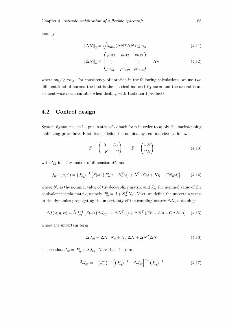
Chapter 4. Attitude stabilization of a flexible spacecraft 68
namely
‖∆N‖2 =√λmax(∆NT∆N) ≤ ρN (4.11)
‖∆N‖ ≤
ρn11 ρn12 ρn13
......
...
ρnM1 ρnM2 ρnM3
= RN (4.12)
where ρnij ≥ νnij . For consistency of notation in the following calculations, we use two
different kind of norms: the first is the classical induced L2 norm and the second is an
element-wise norm suitable when dealing with Hadamard products.
4.2 Control design
System dynamics can be put in strict-feedback form in order to apply the backstepping
stabilizing procedure. First, let us define the nominal system matrices as follows:
F =
(0 IM
−K −C
)B =
(−NCN
)(4.13)
with IM identity matrix of dimension M , and
fn(ω, η, ψ) =(Jneq)−1 [
S(ω)(Jneqω +NT
n ψ)
+NTn (Cψ +Kη − CNnω)
](4.14)
where Nn is the nominal value of the decoupling matrix and Jneq the nominal value of the
equivalent inertia matrix, namely Jneq = J+NTn Nn. Next, we define the uncertain terms
in the dynamics propagating the uncertainty of the coupling matrix ∆N , obtaining:
∆f(ω, η, ψ) = ∆J−1eq
[S(ω)
(∆Jeqω + ∆NTψ
)+ ∆NT (Cψ +Kη − C∆Nω)
](4.15)
where the uncertain term
∆Jeq = ∆NTNn +NTn ∆N + ∆NT∆N (4.16)
is such that Jeq = Jneq + ∆Jeq. Note that the term
∆Jeq = −(Jneq)−1
[(Jneq)−1
+ ∆Jeq
]−1 (Jneq)−1
(4.17)

Chapter 4. Attitude stabilization of a flexible spacecraft 69
comes from the direct application of the matrix inversion lemma to(Jneq + ∆Jeq
)−1. The
kinematic and the dynamics of the flexible spacecraft can thus be written as follows:
ρ = H(ρ)ω (4.18)(η
ψ
)= F
(η
ψ
)+Bω (4.19)
ω = fn(ω, η, ψ) + ∆f(ω, η, ψ) +[(Jneq)−1
+ ∆Jeq
]u (4.20)
Note that the matrix B still contains unmatched model uncertainties, but we will
highlight them later in the design. System (4.18)-(4.19)-(4.20) satisfies the general-
ized matching conditions, thus it is possible to apply the recursive Lyapunov redesign
procedure as one step of robust multi-input backstepping to compensate the unmatched
uncertainties ∆N and ∆f plus compensation of the matched uncertainty ∆Jeq. We
assume to know suitable bounding functions for the uncertain terms, namely
‖∆f(ω, η, ψ)‖ ≤ ρf (ω, η, ψ) (4.21)∥∥∥∆Jeq
∥∥∥1≤ 1
3ρJ 0 ≤ ρJ ≤ 3 (4.22)
where ‖·‖1 stands for the matrix induced L1 norm.
4.2.1 Robust backstepping
Backstepping design is based on the observation that the kinematics and the flexible
dynamics (4.18)-(4.19) can be stabilized by the virtual control law
ωd = −kρ (4.23)
with k ∈ R+. First note that, as a matter of fact, the drift term in equation (4.19) is
globally exponentially stable, since the flexible dynamics is inherently damped. Thus,
there exists a unique, symmetric and positive definite, solution P of the equation
P
(0 I
−K −C
)+
(0 I
−K −C
)TP = −2Q (4.24)
for each fixed matrix Q, symmetric and positive definite. Suppose we know a solution
of the Lyapunov equation (4.24) and let us exploit identity (4.4) to show that, under
the virtual control input (4.23), the kinematic equations are also GES. The closed-loop
kinematic sub-system under virtual control becomes
ρ = −kH(ρ)ρ (4.25)

Chapter 4. Attitude stabilization of a flexible spacecraft 70
Consider now the Lyapunov function
V (ρ) = ρTρ (4.26)
Using (4.4), the derivative of V along the trajectories of (4.25) is given by
V = −2kρTH(ρ)ρ = −2k
(1 + ρTρ
4
)ρTρ ≤ −k
2V (4.27)
which yields global exponential stability with rate of decay k/2. It is then straightforward
to show that, under the same virtual control law (4.23), the whole kinematic plus flexible
sub-system is GES. The “virtual” closed-loop system takes the form
ρ = −kH(ρ)ρ (4.28)(η
ψ
)= F
(η
ψ
)+
(kN
−kCN
)ρ. (4.29)
Define ξ = col(η, ψ) and consider the Lyapunov function
W = V (ρ) + ξTPξ. (4.30)
Evaluating the derivative of W along the trajectories of (4.28)-(4.29), we obtain
W = −kρTH(ρ)ρ+ 2ξTP
[Fξ +
(kN
−kCN
)ρ
]
≤ −k2ρTρ+ 2ξTPFξ + 2ξTP
(kN
−kCN
)ρ
≤ −(ρT ξT
) k
2I 03×2M
2kPB 2Q
︸ ︷︷ ︸
R
(ρ
ξ
)≤ −λmin(R) ‖col(ρ, ξ)‖2
(4.31)
where 03×2M is a block of zeros of dimension 3× 2M, with M number of flexible modes.
Clearly, the matrix R ∈ R(3+2M)×(3+2M) has all positive eigenvalues, hence global expo-
nential stability of the kinematic plus flexible dynamics is established.
Remark 4.2.1.1. Note that the linear control law (4.23) achieves GES of (4.18)-(4.19) irre-
spective of the uncertain decoupling matrix N , thus for all the possible unmatched uncertainties
acting on the kinematic-flexible subsystem. However, since (4.23) is just a virtual control law,
we will have to deal with such unmatched terms in the actual robust backstepping design. ♦

Chapter 4. Attitude stabilization of a flexible spacecraft 71
A graphical interpretation of this result can be given by looking at (4.28)-(4.29) as the
cascade of two GES systems, the first nonlinear and the second linear, as shown in Fig.
4.2.
NONLINEAR GES LINEAR GES
GLOBALLY EXPONENTIALLY STABLE CASCADE
Figure 4.2: The nonlinear GES kinematic sub-system cascaded with the linear GESflexible sub-system yields a nonlinear GES cascade.
Linearity of the “sink” flexible sub-system implies the absence of finite-escape times, thus
avoiding peaking during the transient and ensuring the GES of the cascade. Note that,
if the second subsystem was nonlinear, we should have invoked the stronger property of
input-to-state stability to ensure at least the GAS of the cascade.
The backstepping approach takes advantage of this result by introducing the error co-
ordinate
ζ = ω − ωd = ω + kρ (4.32)
and defining accordingly the mixed state-error system
ρ = H(ρ) [ζ − kρ](η
ψ
)= F
(η
ψ
)+B [ζ − kρ]
ζ = fn(ω, η, ψ) + ∆f(ω, η, ψ) +(Jneq)−1
u+ kH(ρ) [ζ − kρ]
(4.33)
At this first step of the overall design, we disregard the matched uncertainty ∆Jeq.
Since we already know a Lyapunov function W for the (ρ, η, ψ) subsystem, we can build

Chapter 4. Attitude stabilization of a flexible spacecraft 72
a robust control Lyapunov function for (4.33) as follows
U = W (ρ, ξ) +1
2‖ζ‖2 . (4.34)
Evaluating the derivative of (4.34) along the trajectories of (4.33) we can find the ro-
bust backstepping control law which renders U negative definite outside a compact set,
which can be made arbitrarily small by properly choosing some control parameters (P-
RUGAS). The derivative of U takes the form:
U = W (ρ, ξ) + ζT[fn(ω, η, ψ) + ∆f(ω, η, ψ) +
(Jneq)−1
u+ kH(ρ) (ζ − kρ)]
= ρTH(ρ)ζ − kρTH(ρ)ρ+ 2ξTPFξ + 2ξTPBζ − 2kξTPBρ
+ ζT[fn(ω, η, ψ) + ∆f(ω, η, ψ) +
(Jneq)−1
u+ kH(ρ) (ζ − kρ)]
≤ −(ρT ξT
)[kH(ρ) 03×2M
2kPB 2Q
](ρ
ξ
)+ ρTH(ρ)ζ + 2ξTPBnζ + 2ξTP∆Bζ
+ ζT[fn(ω, η, ψ) + ∆f(ω, η, ψ) +
(Jneq)−1
u+ kH(ρ) (ζ − kρ)].
(4.35)
where the local variable ∆B depends solely on ∆N , namely
B = Bn + ∆B =
(−Nn
CNn
)+
(−∆N
C∆N
). (4.36)
The presence of this unmatched uncertainty in inequality (4.35) has to be dealt with
robust backstepping design. We can define a bounding function for ∆B using an element-
wise upper-bound estimate, as done previously for ∆N in (4.12), as follows
‖∆B‖ ≤ ρB
b11 b12 b13
......
...
b2M1 b2M2 b2M3
= RB (4.37)
The control law which solves this first stabilization step is now of straightforward eval-
uation:
uu =− Jneq [fn(ω, η, ψ) + ρf (ω, η, ψ)sigm(ζ, σf ) + kH(ρ) (ζ − kρ)
+HT (ρ)ρ+ 2BTnPξ + 2RTB Σ(ζ, σB)Pξ + kζζ
] (4.38)

Chapter 4. Attitude stabilization of a flexible spacecraft 73
where kζ ∈ R+ is a design gain introduced to force the negativity of U , σB, σf ∈ R+ are
the sigmoid slopes and the vector sigmoid functions take the form
sigm(ζ, σf ) =
sign(ζ1)(1− e−σf |ζ1|)sign(ζ2)(1− e−σf |ζ2|)sign(ζ3)(1− e−σf |ζ3|)
(4.39)
Σ(ζ, σB) =
sign(ζ1)(1− e−σB |ζ1|) · · · sign(ζ1)(1− e−σB |ζ1|)sign(ζ2)(1− e−σB |ζ2|) · · · sign(ζ2)(1− e−σB |ζ2|)sign(ζ3)(1− e−σB |ζ3|) · · · sign(ζ3)(1− e−σB |ζ3|)
(4.40)
Note that Σ(ζ, σB) ∈ R3×2M is introduced for consistency purposes to compensate
the unmatched uncertainty ∆B. For this reason, we need to use the element-wise
(Hadamard) matrix product, identified by the symbol , to bound from above the deriva-
tive of U using the control.
Under (4.38), (4.35) can be reduced to
U ≤−(ρT ξT
)R
(ρ
ξ
)− kζ ‖ζ‖2
+ 2ρBζTBT
n RESB(|ζi|, σB)Pξ + ρf (ω, η, ψ)
3∑i=1
|ζi|e−σf |ζi|(4.41)
where the matrix RESB(|ζi|, σB) ∈ R3×2M has for elements the approximation errors
made in using sigmoid functions instead of discontinuities, namely
RESB(|ζi|, σB) =
sign(ζ1)e−σB |ζ1| · · · sign(ζ1)e−σB |ζ1|
sign(ζ2)e−σB |ζ2| · · · sign(ζ2)e−σB |ζ2|
sign(ζ3)e−σB |ζ3| · · · sign(ζ3)e−σB |ζ3|
. (4.42)
A further simplification of (4.41) leads to
U ≤−(ρT ξT
)R
(ρ
ξ
)− kζ ‖ζ‖2
+ 2ρBresB(|ζi|, σB)Pξ + ρmaxf
3∑i=1
|ζi|e−σf |ζi|(4.43)
where ρmaxf is a upper-bound on ρf for all ω ∈ R3, (η, ψ) ∈ R2M and the row vector
res(|ζi|, σB) ∈ R2M can be expressed as
resB(|ζi|, σB) =(∑3
i=1 b1i|ζi|e−σB |ζi|∑3
i=1 b2i|ζi|e−σB |ζi| · · ·∑3
i=1 b2Mi|ζi|e−σB |ζi|)
(4.44)

Chapter 4. Attitude stabilization of a flexible spacecraft 74
It is easy to show that the terms |ζi|e−σB |ζi| and |ζi|e−σf |ζi| attain a maximum at |ζi| =σ−1B and |ζi| = σ−1
f , respectively. Moreover, since P is known and constant and ξ are
the flexible variables, bounded solutions of a linear damped system, it is again possible
to bound from above U as follows
U ≤−(ρT ξT
)R
(ρ
ξ
)− kζ ‖ζ‖2
+ 2ρBresmax(σB)Pξmax + ρmaxf 3σ−1
f e−1
(4.45)
where
resmax(σB) =(σ−1B e−1
∑3i=1 b1i σ−1
B e−1∑3
i=1 b2i · · · σ−1B e−1
∑3i=1 b2Mi
)(4.46)
Note that the non-negative terms in (4.45) can be shrunk by increasing the sigmoid slopes
σB and σf . Let us rearrange the negative terms defining x = col(ρ, ξ, ζ), obtaining
U ≤ −xT[R 0
0 kζI
]x+ 2ρBresmax(σB)Pξmax + ρmax
f 3σ−1f e−1
≤ −min λmin(R), kζ ‖x‖2 + 2ρBresmax(σB)Pξmax + ρmaxf 3σ−1
f e−1.
(4.47)
As a result, U is negative definite provided that
‖x‖ >
√2ρBresmax(σB)Pξmax + ρmax
f 3σ−1f e−1
min λmin(R), kζ:= Ω(σB, σf ) (4.48)
thus P-RUGAS of the full-state trajectories is established, since they converge to an
“arbitrarily shrinkable” compact set containing the origin.
4.2.2 Recursive Lyapunov redesign
As we have shown in the previous section, the robust backstepping design stabilizes
the flexible spacecraft dynamics by compensating the unmatched uncertainties. To deal
with the matched uncertainty ∆Jeq, of which we know the bounding term ρJ , it is
straightforward to use the recursive Lyapunov redesign introduced in section 3.3. The
robust backstepping control law (4.38) can be expressed as a function of the full-state
x = col(ρ, ξ, ω), namely
uu = ψ(ρ, ξ, ω) = ψ(x). (4.49)

Chapter 4. Attitude stabilization of a flexible spacecraft 75
Moreover, we group system equations and matrices defining
F (x) =
H(ρ)ρ
Fξ +Bω
f(ξ, ω)
G =
03×3
02M×3(Jneq)−1
(4.50)
so that the full flexible-spacecraft dynamics can be expressed as
x = F (x) +G[∆Jequ+ u
](4.51)
Recall that we know a robust control Lyapunov function for system (4.51) in the case
∆Jeq = 0, namely
U(ρ, ξ, ω) = ρTρ+ ξTPξ + ‖ω + kρ‖2 . (4.52)
Under the robust backstepping control law (4.49), U(x) satisfies inequality (4.45), so
that (4.51) is P-RUGAS with ∆Jeq = 0. Moreover, the matched uncertainty ∆Jeq is
such that the inequality∥∥∥∆Jeq(ψ(x) + um)∥∥∥
1≤ ρr(x) +
1
3ρJ ‖um‖1 0 ≤ ρJ < 3 (4.53)
holds, with um recursive Lyapunov redesign control law to be determined and ρr(x) ≥∥∥∥∆Jeqψ(x)∥∥∥
1is a suitable bounding function. Since assumptions 3.3.0.8 and 3.3.0.9
are fulfilled, we can apply the recursive Lyapunov redesign procedure to system (4.51),
which in closed loop with u = ψ(x) + um takes the form
x = f(x) +Gψ(x) +G[∆Jeq (ψ(x) + um) + um
]. (4.54)
Set
(∂U
∂x
)T= w. The derivative of U along the trajectories of (4.54) takes the form
U =
(∂U
∂x
)T(f(x) +Gψ(x)) + w∆Jeq (ψ(x) + um) + wum
≤(∂U
∂x
)T(f(x) +Gψ(x)) + ‖w‖1
∥∥∥∆Jeq (ψ(x) + um)∥∥∥
1+ wum
≤ −min λmin(R), kζ ‖x‖2 + resu(σB, σf ) + ‖w‖1 (ρr(x) + ρJ ‖um‖1) + wum
(4.55)
where resu(σB, σf ) is the residual term in (4.45), namely
resu(σB, σf ) = 2ρBresmax(σB)Pξmax + ρmaxf 3σ−1
f e−1. (4.56)
Setting now
um =ρr(x)
1− ρJsigm(w, σJ) (4.57)

Chapter 4. Attitude stabilization of a flexible spacecraft 76
and accordingly evaluating the induced 1-norms in (4.55), yields
U ≤−min λmin(R), kζ ‖x‖2 + resu(σB, σf )
+ ‖w‖1
[ρr(x) +
1
3ρJ
(3ρr(x)
1− ρJ+
3ρr(x)
1− ρJ
3∑i=1
e−σJ |wi|
)]
+ w
ρr(x)
1− ρJ
sign(w1)e−σJ |w1|
sign(w2)e−σJ |w2|
sign(w3)e−σJ |w3|
− ρr(x)
1− ρJ
sign(w1)
sign(w2)
sign(w3)
(4.58)
Simplifying and taking the maximum values of the residual terms, we obtain
U ≤ −min λmin(R), kζ ‖x‖2 +resu(σB, σf )+9ρJρ
maxr
1− ρJσ−1J e−1 +3
ρmaxr
1− ρJσ−1J e−1 (4.59)
so that the trajectories of the closed-loop system (4.54) converge to the compact set
Ω(σB, σf , σJ) :=
√√√√resu(σB, σf ) + 9 ρJρmaxr
1−ρJ σ−1J e−1 + 3 ρ
maxr
1−ρJ σ−1J e−1
min λmin(R), kζ. (4.60)
P-RUGAS of the origin of (4.54) can thus be concluded. As a result, the flexible space-
craft described by the equations (4.18)-(4.19)-(4.20) is robustly stabilized by the recur-
sive Lyapunov redesign control law u = uu(x) +um(x), with uu(x) defined in (4.38) and
um(x) in (4.57).

Chapter 5
Missile autopilot design
In this chapter, the recursive Lyapunov redesign technique is employed to design the
autopilot of an asymmetric tail-controlled air-to-air missile, in order for it to perform
Skid-To-Turn and Bank-To-Turn maneuvers. After a detailed derivation of the dynami-
cal uncertain model, the problem setting and the construction of a nominal backstepping
controller, we design compensators for the matched and unmatched uncertainties of the
dynamics using the techniques introduced above. The recursive Lyapunov redesign can
handle the uncertainties in the dynamics of a non-minimum phase airframe, thus it is
particularly suited for missile autopilot design. P-RUGAS of the closed-loop system is
shown and several simulations demonstrate the effectiveness of the proposed control law
in different scenarios. The chapter follows the work presented in [86].
5.1 Dynamic model
The missile considered is a very generic, tail-controlled, air-to-air aerodynamic missile
in a non axially-symmetric configuration which allows both Skid-To-Turn and Bank-
To-Turn maneuvers. An example of such an airframe may be Meteor (Fig. 5.1), the
innovative active radar guided beyond-visual-range air-to-air missile (BVRAAM) pro-
duced by MBDA. While wings act as lifting surfaces, the four tail-fins are the control
surfaces which twist and steer the vehicle. The typical use of this kind of missile is that
of intercepting aircraft, anti-aircraft missiles and high-speed ballistic missiles in flight.
The hybrid maneuvering capabilities of the airframe do require an autopilot able to en-
sure tracking of different kind of signals on different dynamic behaviors, with slight or
even none change of the control laws. These requirements can be fulfilled by using the
recursive Lyapunov redesign approach.
The modeling process is based on some quite common assumptions.
77

Chapter 5. Missile autopilot design 78
Figure 5.1: Meteor is an active radar guided beyond-visual-range air-to-air missile(BVRAAM) being developed by MBDA missile systems. Meteor will offer a multi-shotcapability against long range manoeuvring targets in a heavy electronic countermea-sures (ECM) environment with range in excess of 100km. The picture is taken from
defenseindustrydaily.com, all rights reserved c©.
• The considered dynamics is governed by rigid body mechanics, that means flexible
modes due to aeroelasticity are neglected.
• Reference position for aerodynamic data coincides with the center of mass (abbr.
c.o.m.), where all the sensors are mounted.
• Trustworthy measurements or estimates for the angle-of-attack, sideslip angle, an-
gular velocities and bank angle are available through high quality inertial mea-
surement units.
• Thrust force is assumed to be zero, or equivalently fully compensated by drag
force.
• As a consequence of the previous assumption, velocity is assumed to be slowly
varying (increasing) for the first half-window of simulation and constant during
the terminal phase. Wind velocity will be treated as a disturbance.
• Gravity is neglected since it acts on time-scales much longer than those of the
autopilot.

Chapter 5. Missile autopilot design 79
• We also assume constant height of operation h, which determines certain known
thermodynamic characteristics of the local atmosphere, such as constant air density
ρ and speed of sound Vs.
Note that the presence of aeroelastic effects can be treated, as usual, in the frequency-
domain framework, taking care to give the appropriate open-loop attenuation near the
flex-mode frequencies (see, for instance, [94] and [95]). On the other hand, a reference
position shifted from the c.o.m. does not pose a problem, since it can be compensated
by introducing simple correction terms. Furthermore, while the angular velocities are
usually available for feedback, α and β angles need to be estimated somehow, since the
nonlinear control law developed is in the form of full state-feedback. Finally, last four
assumptions are quite usual in autopilot design. In supersonic and hypersonic regimes,
particularly in the terminal phases of the flight, it is not such an issue to consider zero-
gravity conditions and the missile operating in the so-called glide-phase, at zero thrust.
Starting from the Newton linear momentum and the Euler angular momentum laws eval-
uated along the missile body unit-axes (xb, yb, zb)T (body frame fixed on the c.o.m.),
introducing the inertia tensor and differentiating the equations using the Coriolis the-
orem, the 6-DOF equations of motion of a rigid body with slowly varying mass and
inertia are obtained. These six equations are used to represent missile dynamics in the
wind-axes reference frame, after a coordinate transformation [20]. Velocity Vm(t) is as-
sumed to be slowly and linearly increasing in the first part of the simulation window,
according to the following Mach number variation:
M(t) ∈ [2.5, 3.2] (5.1)
in such a way that V0 = 2.5Vs and Vf = 3.2Vs. The second half of the flight envelope is
therefore with constant velocity Vf .
A non axially-symmetric airframe is considered, with inertia matrix (determined con-
sidering the principal inertia axes coincident with the body axes):
I(t) =
Ix(t) 0 −Ixz(t)
0 Iy(t) 0
−Ixz(t) 0 Iz(t)
(5.2)
also slowly time-varying, in particular linearly decreasing in the first part of the flight
envelope due to propellant consumption. For instance, we consider this time profile for

Chapter 5. Missile autopilot design 80
the longitudinal inertia moment:
Ix(t) =
−(Ix0−Ixf
tf
)t+ Ix0 if t ≤ tf
Ixf if t > tf
(5.3)
A similar time evolution has been assigned to the slowly time-varying mass m(t). At
t = tf , when all the propellant has been consumed, the so-called glide-phase starts: the
velocity becomes constant and so the inertia matrix and the mass of the system.
The complete 6-DOF equations of motion are therefore:
ϕ = p
p = Lpqpq + Lqrqr +Iz
IxIz − I2xz
Mx +Ixz
IxIz − I2xz
Mz
q = Mprpr +Mp2p2 +Mr2r
2 +1
IyMy + Cm1pα
r = Npqpq +Nqrqr +Ixz
IxIz − I2xz
Mx +Ix
IxIz − I2xz
Mz + Cm2pβ
α = − cos2(α) tan(β)p+ q − sin(α) cos(α) tan(β)r + Cm3pα+
QαβmVm
Fz + sin(α) cos(α) tan(β)QαβmVm
Fy − sin(α) cos(α)Q2αβ
VmVm
β = cos2(β) tan(α)p+ sin(β) cos(β) tan(α)q − r + Cm4pβ+
QαβmVm
Fy + sin(β) cos(β) tan(α)QαβmVm
Fz − sin(β) cos(β)Q2αβ
VmVm
(5.4)
with
Lpq =Ixz(Ix − Iy + Iz)
IxIz − I2xz
Npq =Ix(Ix − Iy) + I2
xz
IxIz − I2xz
(5.5)
Lqr =Iz(Iy − Iz)− I2
xz
IxIz − I2xz
Nqr =Ixz(Iy − Iz − Ix)
IxIz − I2xz
(5.6)
Mpr =Iz − IxIy
Mp2 = −IxzIy
Mr2 =IxzIy
(5.7)
and
Qαβ =√
1 + tan2(α) + tan2(β) (5.8)
The overall velocity derivative w.r.t. time Vm is thought as an additional input, because
a fixed velocity profile has been imposed. Actually, since it is not going to be taken into
account in control design, it will act as a disturbance. Aerodynamic forces and moments
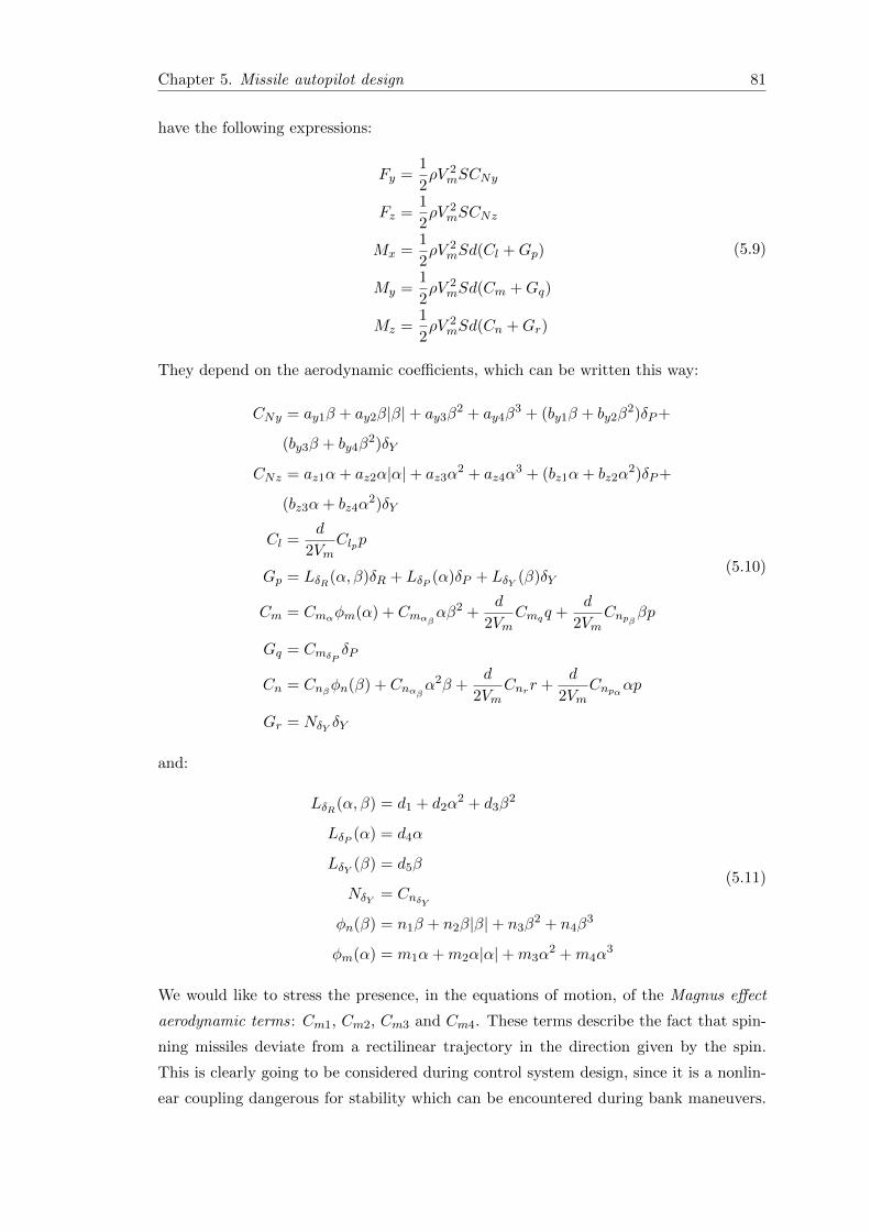
Chapter 5. Missile autopilot design 81
have the following expressions:
Fy =1
2ρV 2
mSCNy
Fz =1
2ρV 2
mSCNz
Mx =1
2ρV 2
mSd(Cl +Gp)
My =1
2ρV 2
mSd(Cm +Gq)
Mz =1
2ρV 2
mSd(Cn +Gr)
(5.9)
They depend on the aerodynamic coefficients, which can be written this way:
CNy = ay1β + ay2β|β|+ ay3β2 + ay4β
3 + (by1β + by2β2)δP+
(by3β + by4β2)δY
CNz = az1α+ az2α|α|+ az3α2 + az4α
3 + (bz1α+ bz2α2)δP+
(bz3α+ bz4α2)δY
Cl =d
2VmClpp
Gp = LδR(α, β)δR + LδP (α)δP + LδY (β)δY
Cm = Cmαφm(α) + Cmαβαβ2 +
d
2VmCmqq +
d
2VmCnpββp
Gq = CmδP δP
Cn = Cnβφn(β) + Cnαβα2β +
d
2VmCnrr +
d
2VmCnpααp
Gr = NδY δY
(5.10)
and:
LδR(α, β) = d1 + d2α2 + d3β
2
LδP (α) = d4α
LδY (β) = d5β
NδY = CnδY
φn(β) = n1β + n2β|β|+ n3β2 + n4β
3
φm(α) = m1α+m2α|α|+m3α2 +m4α
3
(5.11)
We would like to stress the presence, in the equations of motion, of the Magnus effect
aerodynamic terms: Cm1, Cm2, Cm3 and Cm4. These terms describe the fact that spin-
ning missiles deviate from a rectilinear trajectory in the direction given by the spin.
This is clearly going to be considered during control system design, since it is a nonlin-
ear coupling dangerous for stability which can be encountered during bank maneuvers.

Chapter 5. Missile autopilot design 82
The same can be said about the nonlinear cross-couplings which arise between the three
control inputs in the expressions of (5.10). These couplings are produced by the differ-
ential of pressure acting on the wings and tail-fins, a phenomenon particularly relevant
in asymmetric airframes.
Finally, control allocation and actuator dynamics are introduced to make the dynamic
model even more realistic. Control inputs produced by the autopilot have to be trans-
formed in physical reference signals to the four actuated control surfaces placed on the
tail-fins of the missile. In missile dynamics, only the overall deflections produced by the
simultaneous combined deflection of the surfaces are considered, and the same is made
in autopilot design. These three overall deflections are the classical roll, pitch and yaw
ones around the three body axes, namely:
δR = u1
δP = u2
δY = u3
(5.12)
These deflections can be thought as commands to tail-fin dynamics, conceptually sep-
arated in an aileron dynamics, which produces as a final result the roll control torque,
an elevator dynamics, which is the cause of the pitch control torque, and a rudder dy-
namics, producing a yaw control torque. Due to this fact, control inputs generated by
the autopilot are often renamed:
δR = δa (command to aileron dynamics)
δP = δe (command to elevator dynamics)
δY = δr (command to rudder dynamics)
(5.13)
The transformation between these overall control deflections elaborated by the autopilot
and the actual signals to the four wings (δw1, δw2, δw3, δw4)T is represented by the
control allocation matrix : δw1
δw2
δw3
δw4
=
−1 −1 0
−1 0 −1
1 −1 0
1 0 −1
u1
u2
u3
(5.14)
Actuator dynamics on the four fins is an approximation of the fast dynamics of low level
control loops, whose aim is to produce torques on the actuators moving the fins in order
to follow the reference time-profile associated to δwi. After a small time, these low level
control loops achieve their aim and produce the desired torques, giving as output the
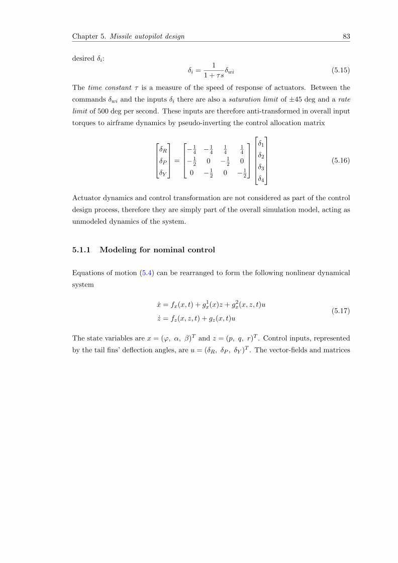
Chapter 5. Missile autopilot design 83
desired δi:
δi =1
1 + τsδwi (5.15)
The time constant τ is a measure of the speed of response of actuators. Between the
commands δwi and the inputs δi there are also a saturation limit of ±45 deg and a rate
limit of 500 deg per second. These inputs are therefore anti-transformed in overall input
torques to airframe dynamics by pseudo-inverting the control allocation matrix
δR
δP
δY
=
−1
4 −14
14
14
−12 0 −1
2 0
0 −12 0 −1
2
δ1
δ2
δ3
δ4
(5.16)
Actuator dynamics and control transformation are not considered as part of the control
design process, therefore they are simply part of the overall simulation model, acting as
unmodeled dynamics of the system.
5.1.1 Modeling for nominal control
Equations of motion (5.4) can be rearranged to form the following nonlinear dynamical
system
x = fx(x, t) + g1x(x)z + g2
x(x, z, t)u
z = fz(x, z, t) + gz(x, t)u(5.17)
The state variables are x = (ϕ, α, β)T and z = (p, q, r)T . Control inputs, represented
by the tail fins’ deflection angles, are u = (δR, δP , δY )T . The vector-fields and matrices

Chapter 5. Missile autopilot design 84
of the system have this structure:
fx(x, t) =
0
fα(x, t)
fβ(x, t)
g1x(x) =
1 0 0
ξα(x) 1 χα(x)
ξβ(x) χβ(x) −1
g2x(x, t) =
0 0 0
0 gα1(x, z, t) gα2(x, z, t)
0 gβ1(x, z, t) gβ2(x, z, t)
fz(x, z, t) =
fp(x, z, t)
fq(x, z, t)
fr(x, z, t)
gz(x, t) =
gp1(x, t) gp2(x, t) gp3(x, t)
0 gq(x, t) 0
gr1(x, t) gr2(x, t) gr3(x, t)
(5.18)
The functions fi, gi, ξi and χi are easily constructed by looking at the dynamics of
(5.4). System (5.17) well represents the complex nonlinear and time-varying behavior
of the missile in the simulation window considered. It involves highly nonlinear non-
stationary aerodynamic terms, mainly in the fi drift terms, highly coupled and nonlinear
differential kinematic terms as g1x(x)z and, furthermore, the cross-couplings between the
control inputs, due to the different pressure acting on the wings and the tail-fins during
maneuvers, especially at high α and β angles. These couplings are going to be taken
into account directly in control system design, using a nonlinear MIMO approach.
For the nominal controller design, system equations are going to be simplified into
x = fx(x) + g1x(x)z
z = fz(x, z) + gz(x)u(5.19)
in which we have dropped the input influence on the second and third equations and we
have made the assumption of constant velocity, mass and inertia during the portion of
flight considered.
5.1.2 Modeling for robust control
The nonlinear dynamical model developed in the previous section is particularly suited
to design nonlinear control laws which are based on cancellations of nominal terms in
system equations. However, it is really difficult to obtain good estimates of aerody-
namic coefficients and Magnus effect terms, which are barely known. Even in the luckier

Chapter 5. Missile autopilot design 85
situations the designer only knows their nominal, often incorrect, value. As a conse-
quence, nonlinear control laws are frequently failing in real applications. This issue led
the control systems research community to think about robust versions of the nonlinear
controllers already available for stabilization and tracking.
To model the very complex aerodynamic uncertain terms of missile dynamics, we need to
exploit the results introduced in Section 2.3 to rapidly evaluate the uncertain envelopes.
As an example of application of proposition 2.3.0.2, let us consider the calculus of the
uncertainty associated to the aerodynamic force Fy. We assume that the air density ρ
and the cross-sectional area S are perfectly known parameters. On the other hand we
group the perturbations deriving from time-variance and uncertainty into the velocity
Vm and the aero-coefficient CNy, of which we only know the nominal values and the
maximum gap k between them and their actual values, according to the specific definition
of deviation function.
Example 5.1.2.1. Consider the nominal expression of the force along yb
Fy =1
2ρV 2
mSCNy
and separate the known part 12ρS = c from the uncertain part V 2
mCNy, which can be
seen as a cubic function of three parameters when written as VmVmCNy. To calculate
the uncertain envelope of Fy we use the ∆ operator in the following fashion
∆(Fy) = ∆(cVmVmCNy) = c∆(VmVmCNy)
= c(∆Vm∆Vm∆CNy + Vm∆Vm∆CNy + ∆VmVm∆CNy+
V 2m∆CNy + ∆Vm∆VmCNy + ∆VmVmCNy + Vm∆VmCNy)
(5.20)
Keeping in mind that it is possible to decompose the single uncertainties in terms of the
deviation function σ and assuming that it is the same for every function, we obtain:
∆(Fy) = σ3Fy + 2σ2Fy + σFy + σ2Fy + 2σFy
= (σ3 + 3σ2 + 3σ)Fy(5.21)
which can be generalized for a generic polynomial nominal function as shown in 2.3.0.2.
Clearly, in the case of a quadratic nominal function, we obtain:
∆(V 2m) = ∆(VmVm) = ∆Vm∆Vm + Vm∆Vm + ∆VmVm
= σ2Vm + σVm + σVm = (σ2 + 2σ)Vm(5.22)
which also fits into 2.3.0.2. ♦

Chapter 5. Missile autopilot design 86
Remark 5.1.2.2. The procedure can be extended to the case of multiple deviation functions.
Since we are limiting ourselves to the case of two different deviation functions for at most three
uncertain parameters in the same uncertain envelope, we show the results in this case, omitting
for brevity the time-dependence of σi’s.
• Two uncertain parameters as in the case of Mx, in which Vm is not squared and Clp
is the other one. The computation of the uncertain envelope gives:
∆(VmClp) = ∆1Vm∆2Clp + Clp∆1Vm + Vm∆2Clp
= (σ1σ2 + σ1 + σ2)VmClp(5.23)
where σ1 embeds the variations of Vm and σ2 those of Clp .
• Three uncertain parameters as in the previous case of Fy. Easy calculations result in:
∆(V 2mCNy) = ∆1Vm∆1Vm∆2CNy + Vm∆1Vm∆2CNy
+ ∆1VmVm∆2CNy + V 2m∆2CNy + ∆1Vm∆1VmCNy
+ ∆1VmVmCNy + Vm∆1VmCNy
= (σ21σ2 + 2σ1σ2 + 2σ1 + σ2 + σ2
1)(V 2mCNy)
(5.24)
♦
Looking at the equations of motions in (5.4) we find out that there are not only products
between uncertain parameters, but also quotients, as in the terms with Vm at denomi-
nator in α and β right members. Therefore, to compute the uncertain envelopes of the
complete dynamics, we also need to use Proposition 2.3.0.3.
The results established in Section 2.3 yield a simple procedure to construct the uncertain
envelopes of system’s vectors and matrices by using the ∆-operator in an element-wise
fashion. Aerodynamic forces and moments are in fact given by products between some
parameters considered known (i.e. scarcely varying around their nominal values), as
S, d, ρ and the inertia moments, and others considered uncertain (i.e. with significant
variations around their nominal values), as Vm (since it embeds all the flight conditions
between 2.5 and 3.2 Mach in a single value), Vm and all the aero-coefficients together with
the Magnus effect terms. The polynomial-in-the-state structure of most aerodynamic
coefficients and their consequent linearity-in-the-parameters implies that the application
of the ∆ operator to each of them results simply in the product of the corresponding
deviation function with the nominal value of the coefficient, as implicitly taken for
granted in the calculations above:
∆(CNy) = σy(t)CNy ∆(CNz) = σz(t)CNz (5.25)

Chapter 5. Missile autopilot design 87
therefore, being σV the perturbation associated to Vm, we have:
∆(Fy) = (σ2V σy + 2σV σy + 2σV + σy + σ2
V )Fy
∆(Fz) = (σ2V σz + 2σV σz + 2σV + σz + σ2
V )Fz(5.26)
furthermore, paying attention to the power of Vm
∆(Mx) =1
4ρSd2p∆(VmClp) +
1
2ρSd∆(V 2
mGp)
= c1(σV σlp + σV + σlp)VmClpp
+ c2(σ2V σGp + 2σV σGp + 2σV + σGp + σ2
V )(V 2mGp)
∆(My) =1
4ρSd2(q∆(VmCmq) + βp∆(VmCnpβ ))
+1
2ρSd(φm(α)∆(V 2
mCmα) + αβ2∆(V 2mCmαβ ) + δP∆(V 2
mCmδP ))
= c1((σV σmq + σV + σmq)VmCmqq + (σV σnpβ + σV + σnpβ )VmCnpββp)
+ c2(φm(α)(σ2V σmα + 2σV σmα + 2σV + σmα + σ2
V )V 2mCmα
+ αβ2(σ2V σmαβ + 2σV σmαβ + 2σV + σmαβ + σ2
V )V 2mCmαβ
+ δP (σ2V σP + 2σV σP + 2σV + σP + σ2
V )V 2mCmδP )
∆(Mz) =1
4ρSd2(r∆(VmCnr) + αp∆(VmCnpα ))
+1
2ρSd(φn(β)∆(V 2
mCnβ ) + α2β∆(V 2mCnαβ ) + δY ∆(V 2
mCnδY ))
= c1((σV σnr + σV + σnr)VmCnrr + (σV σnpα + σV + σnpα )VmCnpααp)
+ c2(φn(β)(σ2V σnβ + 2σV σnβ + 2σV + σnβ + σ2
V )V 2mCnβ
+ α2β(σ2V σnαβ + 2σV σnαβ + 2σV + σnαβ + σ2
V )V 2mCnαβ
+ δY (σ2V σY + 2σV σY + 2σV + σY + σ2
V )V 2mCnδY )
(5.27)
where c1 = 14ρSd
2, c2 = 12ρSd and the various subscripts for σ are needed to distinguish
between different deviation functions. Applying the results of Proposition 2.3.0.3 it is
possible to combine the envelopes found for Fy and Fz with those of Vm and Vm, whose
deviation function is σV . We obtain, i = y, z:
∆
(FiVm
)=Vm∆(Fi)− Fi∆(Vm)
Vm(Vm + ∆(Vm))
=Vm(σ2
V σi + 2σV σi + 2σV + σi + σ2V )Fi − FiσV Vm
Vm(Vm + σV Vm)
∆
(VmVm
)=σV − σV1 + σV
VmVm
(5.28)

Chapter 5. Missile autopilot design 88
Finally, the uncertainties of the Magnus terms are simply ∆(Cmi) = σMiCmi, for i =
1, . . . , 4.
Organizing the uncertain envelopes found by splitting them into drift parts, identified by
the superscript D, depending only on state variables and parameters, and control parts
linear in the control inputs it is straightforward to define the uncertain terms affecting
system’s vector and matrices in the following way:
∆fϕ = 0
∆fα = pασM3Cm3 +Qαβm
∆
(FDzVm
)+ sαcαtβ
Qαβm
∆
(FDyVm
)− sαcαQ2
αβ∆
(VmVm
)
∆fβ = pβσM4Cm4 +Qαβm
∆
(FDyVm
)
+ sβcβtαQαβm
∆
(FDzVm
)− sβcβQ2
αβ∆
(VmVm
)
∆fp =Iz
IxIz − I2xz
∆MDx +
IxzIxIz − I2
xz
∆MDz
∆fq =1
Iy∆MD
y + pασM1Cm1
∆fr =Ixz
IxIz − I2xz
∆MDx +
IxIxIz − I2
xz
∆MDz + pβσM2Cm2
(5.29)
moreover, for i = 1, 2
∆gαi = (σV σαi + σV + σαi)gαi
∆gβi = (σV σβi + σV + σβi)gβi(5.30)
and for j = 1, 2, 3
∆gpj = (σ2V σpj + 2σV σpj + 2σV + σpj + σ2
V )gpj
∆gq = (σ2V σP + 2σV σP + 2σV + σP + σ2
V )gq
∆grj = (σ2V σrj + 2σV σrj + 2σV + σrj + σ2
V )grj
(5.31)
Such uncertain envelopes can be divided in two groups: matched and unmatched uncer-
tainties. The distinction follows the core Definition 2.2.2.1 given in Section 2.2.
Once defined the uncertain terms it is possible to rearrange them into vectors and
matrices to compose a model suited for robust nonlinear control design. Splitting into
the two sub-systems and highlighting the Magnus effect’s terms in ∆fα and ∆fβ with

Chapter 5. Missile autopilot design 89
the purpose of gain more structure, we obtain:
∆fxu =
0
∆f ′α
∆f ′β
+
0 0 0
∆Cm3α 0 0
∆Cm4β 0 0
z
+
0 0 0
0 gα1 + ∆gα1 gα2 + ∆gα2
0 gβ1 + ∆gβ1 gβ2 + ∆gβ2
uM
∆fz =
∆fp
∆fq
∆fr
∆gz =
∆gp1 ∆gp2 ∆gp3
0 ∆gq 0
∆gr1 ∆gr2 ∆gr3
(5.32)
Clearly ∆fxu = ∆fxu(x, z, uM , t), ∆fz = ∆fz(x, z, t) and ∆gz = ∆gz(x, t). We de-
note with uM an estimate for the upper-bound of control inputs vector, considered as
structured uncertainty when it acts on the first part of the dynamics causing the non-
minimum phase behavior of the airframe. The uncertain system then can be expressed
as
x = fx(x, t) + ∆fxu(x, z, uM , t) + g1x(x)z
z = fz(x, z, t) + ∆fz(x, z, t) + [gz(x, t) + ∆gz(x, t)]u(5.33)
Note that, disregarding the uncertain terms and the explicit time-dependence of system’s
equations, this model reduces to the nominal one (5.19).
The unmatched uncertainties ∆fu are those acting directly on f :
∆fu(x, z, uM , t) =
(∆fxu(x, z, uM , t)
∆fz(x, z, t)
)(5.34)
while the matched uncertainties ∆gm appear in the same channel of the control inputs
∆gm(x, t) =
(0 0
0 ∆gz(x, t)
)(5.35)
This system representation will be used to design robust control once defined the bound-
ing functions of the uncertain terms, which are of straightforward calculation using the
properties of the deviation functions introduced in Section 2.2. For instance, we can eval-
uate the bounds of the uncertainties on FDy and FDz by simply replacing the deviation
functions with the corresponding gains kV , ky and kz
ρFDy = (k2V ky + 2kV ky + 2kV + ky + k2
V )|FDy |
ρFDz = (k2V kz + 2kV kz + 2kV + kz + k2
V )|FDz |(5.36)

Chapter 5. Missile autopilot design 90
The same can be done for the Magnus effect terms, for which we obtain, i = 1, . . . , 4:
ρCmi = kMi|Cmi| (5.37)
Similar but much more complicated expressions, which we omit for brevity since their
calculation is also straightforward, can be found for ∆MDx , ∆MD
y and ∆MDz , resulting
in bounding functions ρMDx
, ρMDy
and ρMDz
. Furthermore it is possible to define the
bounding functions for the terms ∆(FDiVm
)and ∆
(VmVm
), for i = y, z, as:
ρFDi /Vm=
∣∣∣∣∣VmρFDi − FikV |Vm|)Vm(Vm + kV |Vm|)
∣∣∣∣∣ρVm/Vm =
∣∣kV − kV ∣∣1 + kV
∣∣∣∣∣ VmVm∣∣∣∣∣
(5.38)
After the derivation of these critical bounds, it is pretty simple to calculate the bounding
functions ρfi of all the uncertain envelopes introduced in (5.29), i = α, β, p, q, r. We give
just the example of calculus of ρfα , because the other ones are very similar to this.
|∆fα| ≤ ρfα =
∣∣∣∣pαkM3|Cm3|+Qαβm
ρFDz /Vm
+sαcαtβQαβm
ρFDy /Vm − sαcαQ2αβρVm/Vm
∣∣∣∣ (5.39)
Finally, we can evaluate bounding functions for (5.30), i = 1, 2, and (5.31), j = 1, 2, 3:
|∆gαi| ≤ ρgαi = (kV kαi + kV + kαi)|gαi|
|∆gβi| ≤ ρgβi = (kV kβi + kV + kβi)|gβi|
|∆gpj | ≤ ρgpj = (k2V kpj + 2kV kpj + 2kV + kpj + k2
V )|gpj |
|∆gq| ≤ ρgq = (k2V kP + 2kV kP + 2kV + kP + k2
V )|gq|
|∆grj | ≤ ρgrj = (k2V krj + 2kV krj + 2kV + krj + k2
V )|grj |
(5.40)
Remark 5.1.2.3. The values of the gains ki are chosen to the extent of size-domination of
the particular uncertain terms considered. Together with the choice of the overall ρi bounding
functions, they determine the level of robustness and associated conservatism of the closed-loop
system under the robust nonlinear control. For instance, choosing the ki gains exactly equal
to the deviation functions amplitudes guarantees the right compromise between robustness and
performance, since no extra-effort than that closely needed is put into uncertainty compensa-
tion. ♦
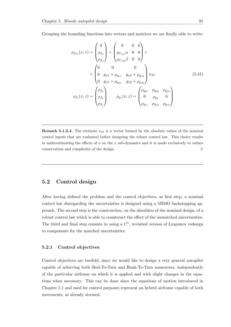
Chapter 5. Missile autopilot design 91
Grouping the bounding functions into vectors and matrices we are finally able to write:
ρfxu(x, z) =
0
ρfα
ρfβ
+
0 0 0
ρCm1α 0 0
ρCm2β 0 0
z
+
0 0 0
0 gα1 + ρgα1 gα2 + ρgα2
0 gβ1 + ρgβ1 gβ2 + ρgβ2
uM
ρfz(x, z) =
ρfp
ρfq
ρfr
ρgz(x, z) =
ρgp1 ρgp2 ρgp3
0 ρgq 0
ρgr1 ρgr2 ρgr3
(5.41)
Remark 5.1.2.4. The estimate uM is a vector formed by the absolute values of the nominal
control inputs that are evaluated before designing the robust control law. This choice results
in underestimating the effects of u on the x sub-dynamics and it is made exclusively to reduce
conservatism and complexity of the design. ♦
5.2 Control design
After having defined the problem and the control objectives, as first step, a nominal
control law disregarding the uncertainties is designed using a MIMO backstepping ap-
proach. The second step is the construction, on the shoulders of the nominal design, of a
robust control law which is able to counteract the effect of the unmatched uncertainties.
The third and final step consists in using a C1, revisited version of Lyapunov redesign
to compensate for the matched uncertainties.
5.2.1 Control objectives
Control objectives are twofold, since we would like to design a very general autopilot
capable of achieving both Skid-To-Turn and Bank-To-Turn maneuvers, independently
of the particular airframe on which it is applied and with slight changes in the equa-
tions when necessary. This can be done since the equations of motion introduced in
Chapter 5.1 and used for control purposes represent an hybrid airframe capable of both
movements, as already stressed.

Chapter 5. Missile autopilot design 92
The problem of controlling the motion of a missile achieving maneuvers can be inter-
preted as the problem of achieving P-RUGAS of a nonlinear uncertain system using an
opportune control law. As a consequence, we are able now to formulate the two control
problems to be solved in terms of the two main maneuvers.
Skid-To-Turn maneuver
The autopilot has to rapidly steer the bank angle ϕ to a constant desired value (usually
zero or near zero) and so to bring to zero the roll-rate p for the purpose of inertially
decoupling the longitudinal from the lateral motion. This is not necessary since the
approach is nonlinear, but it is a common practice. We could also track a time-varying
motion in ϕ, but this would not correspond to the typical STT maneuver we want to
make. Once the bank angle is regulated, rapidly changing time-profiles in α and β have
to be tracked to guarantee the pursuit of the desired vertical and lateral commanded
accelerations, respectively az and ay, produced by the guidance system. Viewed in terms
of P-RUGAS, control objectives for the STT maneuver are:
ϕ(t)→ ωϕ(ϕd) = ωϕ(0)
α(t)→ ωα(αd(t))
β(t)→ ωβ(βd(t))
(5.42)
ωi represent the limit sets of convergence of the state trajectories: according to Def.
1.3.2.2 they can be made arbitrarily small through an opportune choice of control design
parameters; we will show this peculiarity in the next sections.
Bank-To-Turn maneuver
The autopilot has to rapidly steer the sideslip angle β to a constant desired value (usually
zero or near zero) and so to bring to zero the yaw-rate r to prevent the air-breathing
engine typical of BTT missiles from flaming out. The first part of the maneuver, the
twisting, consists in reaching the desired value of ϕ corresponding to the direction of the
commanded acceleration in terms of ay and az. Secondly, the missile has to gain the
desired angle of attack, given by the desired acceleration magnitude in that direction:
this is called the steering part of the maneuver. Viewed in terms of P-RUGAS, control
objectives for the STT maneuver are:
β(t)→ ωβ(βd) = ωβ(0)
ϕ(t)→ ωϕ(ϕd(t))
α(t)→ ωα(αd(t))
(5.43)

Chapter 5. Missile autopilot design 93
5.2.2 Nominal control law
To apply backstepping we start from (5.19), which has a suitable structure, and define
the error variable ex = xd − x, that incorporates the desired values of α, β and ϕ
according to the selected maneuver. Suppose there exists a function φ(x) such that the
error-subsystem
ex = xd − x = xd − fx(x)− g1x(x)φ(x) (5.44)
is globally asymptotically stable (abbr. GAS ) with a Lyapunov function V (ex). This
means that
V (ex) =∂V
∂ex
(xd − fx(x)− g1
x(x)φ(x))≤ −w(‖ex‖) (5.45)
where w(·) is a class K∞ function (see [62]). Define the following change of coordinates
ζ = z − φ(x) (5.46)
under which the system can be written in terms of the error ζ between the virtual control
input z and its desired value zd = φ(x)
ex = xd − fx(x)− g1x(x) (ζ + φ(x))
ζ = fz(x, z) + gz(x)u− ∂φ
∂x
[fx(x) + g1
x(x) (ζ + φ(x))] (5.47)
The obtained representation is mixed in ex, x, z and ζ. Define now the augmented
Lyapunov function
W (ex, ζ) = V (ex) +1
2ζT ζ (5.48)
which is a candidate Lyapunov function for the transformed system (5.47). The deriva-
tive along the motion
W (x, ζ) =∂V
∂ex
[xd − fx(x)− g1
x(x) (ζ + φ(x))]
+ ζT[fz(x, z) + gz(x)u− ∂φ
∂x
(fx(x) + g1
x(x) (ζ + φ(x)))]
≤ −w(‖ex‖)−∂V
∂exg1x(x)ζ
+ ζT[fz(x, z) + gz(x)u− ∂φ
∂x
(fx(x) + g1
x(x) (ζ + φ(x)))]
(5.49)
is made negative definite by the following choice of u:
u = g−1z (x)
[−fz(x, z) +
∂φ
∂x
(fx(x) + g1
x(x) (ζ + φ(x)))
+
(∂V
∂exg1x(x)
)T−Kζζ
] (5.50)

Chapter 5. Missile autopilot design 94
which yields:
W (x, ζ) ≤ −w(‖ex‖)− ζTKζζ (5.51)
A possible choice for φ(x) is that of a dynamic cancellation with eigenvalue assignment
to the error dynamics:
φ(x) =[g1x(x)
]−1(−fx(x) + xd +Kxex) (5.52)
With this choice, the simple quadratic-in-the-error Lyapunov function
V (ex) =1
2eTx ex (5.53)
ensures GAS for the error dynamics. The closed loop system(ex
ζ
)=
(−Kx −g1
x(x)
g1x(x)T −Kζ
)(ex
ζ
)(5.54)
is then GAS with Lyapunov function W (ex, ζ) = 12eTx ex + 1
2ζT ζ, such that W (ex, ζ) ≤
−eTxKxex − ζTKζζ with the (nominal) control law (5.50).
Remark 5.2.2.1. The approach used is called backstepping since it is recursive and exploits
the concept of virtual control (φ(x) in our case) to stabilize the inner part of the dynamics,
in some sense stepping back from the last subsystem up to the first. The recursion is given
by the change of coordinates, which can be extended to more complex systems that still have
a lower-triangular structure, called strict-feedback form. This change of coordinates allows for
the construction of a non-quadratic (in the original coordinates) Lyapunov function, making the
problem of finding a globally stabilizing control law for the whole system much easier. ♦
This first result only implies that the nominal system, with the uncertain terms kept
to zero, is GAS. To ensure P-RUGAS of the uncertain system we need to make the
backstepping robust against both matched and unmatched uncertainties.
5.2.3 Robust nonlinear control
The robustification of (5.50) is split up into two parts: the first is the construction of a
control law uu to counteract unmatched uncertainties and the second is the determina-
tion of another term um which can face the effects of matched uncertainties. Renaming

Chapter 5. Missile autopilot design 95
(5.50) as un, the overall robust nonlinear control law will have the form:
u = un + uu + um (5.55)
Unmatched control
Unmatched control, otherwise known as robust backstepping, is built “on the shoulder”
of the nominal design, from which inherits recursion and virtual control concepts. In
order to compensate for the unmatched uncertain terms, we exploit the concept of robust
control function, introduced in Definition 3.1.0.4, which we adapt to the present context
with the following straightforward element-wise extension
Definition 5.2.3.1 (Element-wise robust control function). The robust control function
can be extended to a vector context by smartly using both matrix product and the element-wise
vector and matrix Hadamard product, denoted by the symbol “”. For instance, if ρu is a three-
dimensional vector of uncertain terms and so are the independent variables s and σs, we define
the element-wise robust control function as follows:
ρu v(s, σs) = ρu sign(s) (1− e−σs|s|) = ρu sigm(s, σs) (5.56)
where
1 =(
1 1 1)T
sign(s) =(
sign(s1) sign(s2) sign(s3))T
e−σs|s| =(e−σs1
|s1| e−σs2|s2| e−σs3
|s3|)T (5.57)
and, as a consequence:
sigm(s, σs) =
sigm(s1)
sigm(s2)
sigm(s3)
=
sign(s1)
sign(s2)
sign(s3)
1− e−σs1|s1|
1− e−σs2|s2|
1− e−σs3|s3|
(5.58)
♦
We consider this model for unmatched control design:
x = fx(x) + ∆fxu(x, z, u, t) + g1x(x)z
z = fz(x, z) + ∆fz(x, z, t) + gz(x)u(5.59)
and prove the following result on trajectory tracking using robust backstepping in the
presence of unmatched uncertainties.

Chapter 5. Missile autopilot design 96
Theorem 5.2.3.2. Given the system with unmatched uncertainties (5.59), the robust backstep-
ping control law :
u′ = un + uu
= geqz (x, z)−1
[(eTx g
1x(x))T − feqz (x, z) +
∂φr∂x
(xd +Kxex + g1
x(x)ζ)
−Kζζ − ρeqfz sigm(ζ) +∂φr(x)
∂xρfxu (1− sigm(ex))
] (5.60)
where
geqz (x, z) = gz(x)− ∂φr∂z
gz(x) feqz = fz −∂φr∂z
fz(x) (5.61)
and ρeqfz is the bounding function of the equivalent uncertainty ∆feqz = ∆fz− ∂φr
∂z ∆fz(x), together
with the robust virtual control input:
φr(x, z) =[g1x(x)
]−1(−fx(x) + xd +Kxex − ρfxu(x, z) sigm(ex)) (5.62)
and robust control Lyapunov function (depending on ζ = z − φr(x, z)):
Wr(ex, ζ) =1
2eTx ex +
1
2ζT ζ (5.63)
renders the closed-loop system (5.59)-(5.60) P-RUGAS about the desired trajectory xd(t) =
(ϕd(t), αd(t), βd(t)). ♦
Proof. The partial change of coordinates:(x
ζ
)=
(x
z − φr(x, z)
)(5.64)
transforms system (5.59) into the following mixed representation:
x = fx(x) + ∆fxu + g1x(x) (ζ + φr(x, z))
ζ = fz(x, z) + ∆fz + gz(x)u
− ∂φr∂x
[fx(x) + ∆fxu + g1
x(x) (ζ + φr(x, z))]
− ∂φr∂z
[fz(x, z) + ∆fz + gz(x)u]
(5.65)

Chapter 5. Missile autopilot design 97
which, by substituting the expression of the robust fictitious control φr(x, z) (first step
of the procedure), can be simplified into:
x = xd +Kxex + g1x(x)ζ + ∆fxu − ρfxu(x, z) sigm(ex)
ζ = feqz (x, z) + ∆feqz + geqz (x, z)u
− ∂φr∂x
[xd +Kxex + g1
x(x)ζ + ∆fxu − ρfxu(x, z) sigm(ex)] (5.66)
In the second step, we close the loop by applying the actual control law (5.60) which,
keeping in mind that ex = xd − x, yields:
ex = −Kxex − g1x(x)ζ + ∆fxu − ρfxu sigm(ex)
ζ =(eTx g
1x(x)
)T+ ∆feqz − ρ
eqfz sigm(ζ)
− ∂φr∂x
(∆fxu − ρfxu sigm(ex))
+∂φr∂x
ρfxu (1− sigm(ex))−Kζζ
(5.67)
We now apply Lyapunov direct criterion to show that (5.67) is P-RUGAS. The aug-
mented candidate Lyapunov function we choose is Wr(ex, ζ) = 12eTx ex + 1
2ζT ζ. Its
derivative along the trajectories of (5.67) is:
Wr(ex, ζ) = eTx ex + ζT ζ
= −eTxKxex − eTx g1x(x)ζ + eTx (∆fxu − ρfxu sigm(ex))
+ ζT(eTx g
1x(x)
)T+ ζT
(∆feqz − ρ
eqfz sigm(ζ)
)− ζT ∂φr
∂x(∆fxu − ρfxu sigm(ex))
+ ζT∂φr∂x
ρfxu (1− sigm(ex))− ζTKζζ
= −eTxKxex − ζTKζζ + eTx∆fxu − (ex sign(ex))Tρfxu
+ (ex sign(ex))Tρfxu e−σx|ex| + ζT∆feqz − (ζ sign(ζ))Tρeqfz
+ (ζ sign(ζ))Tρeqfz e−σζ|ζ| − ζT ∂φr∂x
∆fxu + ζT∂φr∂x
ρfxu
(5.68)
in which we have used commutativity and associativity of the Hadamard product. In
the following, we define in tensorial notation the vector given by the absolute values of
ex and ζ components, which is clearly related to the L1 norm structure:
(ex sign(ex))T = |ex|T =(|ex1 | |ex2 | |ex3 |
)T(ζ sign(ζ))T = |ζ|T =
(|ζ1| |ζ2| |ζ3|
)T (5.69)
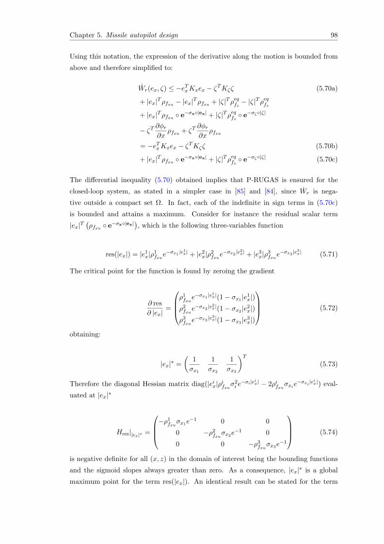
Chapter 5. Missile autopilot design 98
Using this notation, the expression of the derivative along the motion is bounded from
above and therefore simplified to:
Wr(ex, ζ) ≤ −eTxKxex − ζTKζζ (5.70a)
+ |ex|Tρfxu − |ex|Tρfxu + |ζ|Tρeqfz − |ζ|Tρeqfz
+ |ex|Tρfxu e−σx|ex| + |ζ|Tρeqfz e−σζ|ζ|
− ζT ∂φr∂x
ρfxu + ζT∂φr∂x
ρfxu
= −eTxKxex − ζTKζζ (5.70b)
+ |ex|Tρfxu e−σx|ex| + |ζ|Tρeqfz e−σζ|ζ| (5.70c)
The differential inequality (5.70) obtained implies that P-RUGAS is ensured for the
closed-loop system, as stated in a simpler case in [85] and [84], since Wr is nega-
tive outside a compact set Ω. In fact, each of the indefinite in sign terms in (5.70c)
is bounded and attains a maximum. Consider for instance the residual scalar term
|ex|T(ρfxu e−σx|ex|
), which is the following three-variables function
res(|ex|) = |e1x|ρ1
fxue−σx1 |e
1x| + |e2
x|ρ2fxue
−σx2 |e2x| + |e3
x|ρ3fxue
−σx3 |e3x| (5.71)
The critical point for the function is found by zeroing the gradient
∂ res
∂ |ex|=
ρ1fxue−σx1 |e
1x|(1− σx1 |e1
x|)ρ2fxue−σx2 |e
2x|(1− σx2 |e2
x|)ρ3fxue−σx3 |e
3x|(1− σx3 |e3
x|)
(5.72)
obtaining:
|ex|∗ =
(1
σx1
1
σx2
1
σx3
)T(5.73)
Therefore the diagonal Hessian matrix diag(|eix|ρifxuσ2i e−σi|eix| − 2ρifxuσxie
−σxi |eix|) eval-
uated at |ex|∗
Hres||ex|∗ =
−ρ1
fxuσx1e
−1 0 0
0 −ρ2fxuσx2e
−1 0
0 0 −ρ3fxuσx3e
−1
(5.74)
is negative definite for all (x, z) in the domain of interest being the bounding functions
and the sigmoid slopes always greater than zero. As a consequence, |ex|∗ is a global
maximum point for the term res(|ex|). An identical result can be stated for the term
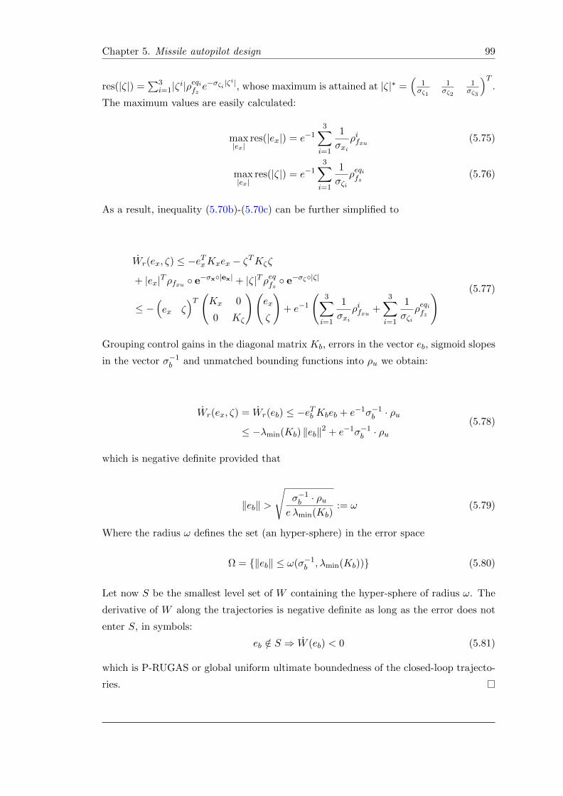
Chapter 5. Missile autopilot design 99
res(|ζ|) =∑3
i=1|ζi|ρeqifze−σζi |ζ
i|, whose maximum is attained at |ζ|∗ =(
1σζ1
1σζ2
1σζ3
)T.
The maximum values are easily calculated:
max|ex|
res(|ex|) = e−13∑i=1
1
σxiρifxu (5.75)
max|ex|
res(|ζ|) = e−13∑i=1
1
σζiρeqifz (5.76)
As a result, inequality (5.70b)-(5.70c) can be further simplified to
Wr(ex, ζ) ≤ −eTxKxex − ζTKζζ
+ |ex|Tρfxu e−σx|ex| + |ζ|Tρeqfz e−σζ|ζ|
≤ −(ex ζ
)T (Kx 0
0 Kζ
)(ex
ζ
)+ e−1
(3∑i=1
1
σxiρifxu +
3∑i=1
1
σζiρeqifz
) (5.77)
Grouping control gains in the diagonal matrix Kb, errors in the vector eb, sigmoid slopes
in the vector σ−1b and unmatched bounding functions into ρu we obtain:
Wr(ex, ζ) = Wr(eb) ≤ −eTb Kbeb + e−1σ−1b · ρu
≤ −λmin(Kb) ‖eb‖2 + e−1σ−1b · ρu
(5.78)
which is negative definite provided that
‖eb‖ >
√σ−1b · ρu
e λmin(Kb):= ω (5.79)
Where the radius ω defines the set (an hyper-sphere) in the error space
Ω = ‖eb‖ ≤ ω(σ−1b , λmin(Kb)) (5.80)
Let now S be the smallest level set of W containing the hyper-sphere of radius ω. The
derivative of W along the trajectories is negative definite as long as the error does not
enter S, in symbols:
eb /∈ S ⇒ W (eb) < 0 (5.81)
which is P-RUGAS or global uniform ultimate boundedness of the closed-loop trajecto-
ries.

Chapter 5. Missile autopilot design 100
Remark 5.2.3.3. The dimension of the set Ω, and so the dimension of S, can be reduced by
acting on the gains in Kb and on the sigmoid slopes, as shown by the expression of the radius
(5.79). Otherwise, we can use the Hadamard product to derive an alternative version of (5.78)
in terms of the following elementwise inequalities, i = 1, 2, 3
|exi| >
√ρifxu
kxiσxi
e(5.82)
|ζi| >
√ρeqifz
kζi σζi e(5.83)
which are chosen using a more conservative upper estimate than that of (5.79), but give more
degrees of freedom and flexibility to the design, since it is possible to individually set control
gains and sigmoid slopes for each error component. ♦
Matched control
Matched uncertainties are finally compensated using a revisited version of a classic
Lyapunov redesign technique (see [62] for the details). The model used for matched
control design is simply derived from (5.33), disregarding the time dependence in the
nominal part:
x = fx(x) + ∆fxu(x, z, u, t) + g1x(x)z
z = fz(x, z) + ∆fz(x, z) + gz(x)[I3 + ∆g′z(x, t)
]u
(5.84)
whereas, clearly by definition of matched uncertainty:
∆g′z(x, t) = g−1z (x)∆gz(x, t) (5.85)
Lyapunov redesign is usually built on the shoulders of a control law and a Lyapunov
function which work for a system without uncertainties. Our extension is instead based
on the unmatched control law (5.60), u′, which is already a robust control law, and on
the associated robust control Lyapunov function Wr. We define the final control law as
the sum of the nominal plus unmatched law u′ with the matched law um
u = u′ + um (5.86)
In addition to the assumption of ∆gz being a matched uncertainty, we need a further
hypothesis which is strictly related to the already stated matching condition, in order
to avoid problems given by a possibly unknown control direction.

Chapter 5. Missile autopilot design 101
Assumption 5.2.3.4. The following inequality holds for the matched uncertainty:
∥∥∆g′z(x, t)u∥∥ =
∥∥∆g′z(x, t)(u′(x, z) + um
)∥∥≤∥∥∆g′z(x, t)u
′(x, z)∥∥+
∥∥∆g′z(x, t)∥∥ ‖um‖ ≤ ρLR(x, z) + k0 ‖um‖
(5.87)
where, as intuition suggests, ρLR(x, z, t) ≥ ‖∆g′z(x, t)u′(x, z)‖ is the Lyapunov redesign
bounding function, and k0 ≥ ‖∆g′z(x, t)‖ is a scalar design parameter which takes values
in the interval [0, 1). ♦
Clearly assumption 5.2.3.4 can be satisfied only if ‖∆g′z(x, t)‖ < 1 and easy calculations
show that this is the case if the bounding functions in ρgz , taken for simplicity with a
single deviation function, are such that k < −1 +√
(2). If this is true, the following
inequalities hold:
∥∥∆g′z(x, t)∥∥ ≤ ∥∥g−1
z (x)∥∥ ‖∆gz(x, t)‖ ≤ ∥∥g−1
z (x)∥∥ ‖ρgz(x)‖ (5.88)
and assumption 5.2.3.4 is fulfilled. The condition on K clearly limits the maximum
amount of matched uncertainty that can be compensated by um, whose standard ex-
pression is the following:
um = −η(x, z, t)
1− k0· w
‖w‖(5.89)
where η(x, z, t) ≥ ρLR(x, z, t) in the domain of interest and
wT =∂Wr
∂(ex, ζ)
(g2x(x)
gz(x)
)= eTx g
2x(x) + ζT gz(x)
This control law is discontinuous for w = 0, thus potentially bringing serious implemen-
tation problems like chattering. This issue is bypassed using once again the elementwise
sigmoid function, which has continuous first derivative. As a result, the complete robust
control law is
u = u′ + um
= geqz (x, z)−1
[(eTx g
1x(x))T − feqz (x, z) +
∂φr∂x
(xd +Kxex + g1
x(x)ζ)
−Kζζ − ρeqfz sigm(ζ) +∂φr∂x
ρfxu (1− sigm(ex))
]− η(x, z, t)
1− k0sigm(w)
(5.90)

Chapter 5. Missile autopilot design 102
5.3 Simulation and results
Simulations are made in MATLAB-Simulink c©environment. Two different maneuvers
have to be pursued by the missile in order to compare the two controllers (simple non-
linear backstepping and robust backstepping) performances in several scenarios with
different amounts of uncertainty.
The values of the parameters describing the airframe are listed in tab. 5.1
Table 5.1: Missile airframe parameters
Symbol Definition Value Unit
m0 mass at t0 185 KgIx0 inertia moment at t0 0.73 Kg ·m2
Iy0, Iz0 inertia moments at t0 205.7 Kg ·m2
Ixz0 inertia moment at t0 0.42 Kg ·m2
Ixf inertia moment at tf 0.64 Kg ·m2
Iyf , Izf inertia moments at tf 180.73 Kg ·m2
Ixzf inertia moment at tf 0.38 Kg ·m2
mf mass at tf 137.5 Kgl fuselage length 3.65 md fuselage diameter 0.178 mS reference area 0.0249 m2
M Mach number [2.5, 3.2] -
V s nominal speed of sound 285.4 m/sρ nominal air density 0.542 Kg/m3
τ actuator dynamics time-constant 5 ms
5.3.1 Skid-To-Turn maneuver
The first maneuver performed is the Skid-To-Turn, which requires less effort from the
controller, since it does not enhance the couplings and nonlinearities of the airframe
dynamics. Both controllers are tested in two scenarios, the first with the 30 % of
uncertainty and the second, harder to be dealt with, with the 60 % of deviation from
the nominal parameters’ values.
Nominal controller The nominal controller behaves good when dealing with low un-
certainty, ensuring a rapid convergence to the desired trajectories with small overshoots
and control effort. However, increasing the level of the perturbation results in too big
deviations from the reference signals and so in a dangerously peaking control signal. In
this second scenario the level of performance is clearly unsatisfactory and the nominal
autopilot is not able anymore to follow the acceleration commands produced by the
guidance system (Fig. 5.2, 5.3, 5.4, 5.5).

Chapter 5. Missile autopilot design 103
0 0.2 0.4 0.6 0.8 1 1.2 1.4 1.6 1.8 2−1
−0.5
0
0.5
1
1.5Angle of Attack tracking response at two different levels of uncertainty: nominal controller
t
α(t)
ref30%60%
Figure 5.2: STT maneuver - Angle of Attack tracking response at two different levelsof uncertainty: nominal controller.
0 0.2 0.4 0.6 0.8 1 1.2 1.4 1.6 1.8 2−1.5
−1
−0.5
0
0.5
1Angle of Sideslip tracking response at two different levels of uncertainty: nominal controller
t
β(t)
ref30%60%
Figure 5.3: STT maneuver - Angle of Sideslip tracking response at two different levelsof uncertainty: nominal controller.
0 0.2 0.4 0.6 0.8 1 1.2 1.4 1.6 1.8 2−0.2
−0.1
0
0.1
0.2
0.3
0.4
0.5Bank Angle regulation response at two different levels of uncertainty: nominal controller
t
φ(t)
ref30%60%
Figure 5.4: STT maneuver - Bank Angle regulation response at two different levelsof uncertainty: nominal controller.

Chapter 5. Missile autopilot design 104
0 0.2 0.4 0.6 0.8 1 1.2 1.4 1.6 1.8 20
0.5
1
1.5
2
2.5x 10
4 Norm of the control inputs vector at two different levels of uncertainty: nominal controller
t
||u(t
)||
30%
60%
Figure 5.5: STT maneuver - Norm of the control inputs vector at two different levelsof uncertainty: nominal controller.
Robust controller The robust controller behaves good in both scenarios, with a level of
performance a bit poorer when uncertainty is at 60 %, nevertheless maintaining precision
and speed of response sufficient to achieve guidance objectives. In the 60 % scenario
it should be highlighted the very nervous transient in the control inputs, which is a
somewhat structural feature of the robust nonlinear approaches [32] (Fig. 5.6, 5.7, 5.8,
5.9).
0 0.2 0.4 0.6 0.8 1 1.2 1.4 1.6 1.8 2−0.8
−0.6
−0.4
−0.2
0
0.2
0.4
0.6
0.8Angle of Attack tracking response at two different levels of uncertainty: robust controller
t
α(t)
ref30%60%
Figure 5.6: STT maneuver - Angle of Attack tracking response at two different levelsof uncertainty: robust controller.
Comparison A comparison between the two closed-loop behaviors shows the superiority
of the robust nonlinear approach in both scenarios, since it ensures higher tracking
precision at lower energy (propellant) consumption (Fig. 5.10, 5.11).

Chapter 5. Missile autopilot design 105
0 0.2 0.4 0.6 0.8 1 1.2 1.4 1.6 1.8 2−0.8
−0.6
−0.4
−0.2
0
0.2
0.4
0.6Angle of Sideslip tracking response at two different levels of uncertainty: robust controller
t
β(t)
ref30%60%
Figure 5.7: STT maneuver - Angle of Sideslip tracking response at two different levelsof uncertainty: robust controller.
0 0.2 0.4 0.6 0.8 1 1.2 1.4 1.6 1.8 2−0.05
0
0.05
0.1
0.15
0.2
0.25
0.3
0.35
0.4
0.45Bank Angle regulation response at two different levels of uncertainty: robust controller
t
φ(t)
ref30%60%
Figure 5.8: STT maneuver - Bank Angle regulation response at two different levelsof uncertainty: robust controller.
0 0.2 0.4 0.6 0.8 1 1.2 1.4 1.6 1.8 20
200
400
600
800
1000
1200Norm of the control inputs vector at two different levels of uncertainty: robust controller
t
||u(t
)||
30%
60%
Figure 5.9: STT maneuver - Norm of the control inputs vector at two different levelsof uncertainty: robust controller.

Chapter 5. Missile autopilot design 106
0 0.2 0.4 0.6 0.8 1 1.2 1.4 1.6 1.8 20
0.2
0.4
0.6
0.8
1
1.2
1.4Norm of the tracking error vector at low uncertainty: comparison between nominal and robust controllers
t||e
x(t)|
|
0 0.2 0.4 0.6 0.8 1 1.2 1.4 1.6 1.8 20
1
2
3
4x 10
5 Energy of the control inputs vector at low uncertainty: comparison between nominal and robust controllers
t
\int |
|u(t
)||^
2 \ d
t
nominal controller
robust controller
nominal controller
robust controller
Figure 5.10: STT maneuver - Norm of the tracking error vector and energy of thecontrol inputs vector at low uncertainty: comparison between nominal and robust con-
trollers
0 0.2 0.4 0.6 0.8 1 1.2 1.4 1.6 1.8 20
0.5
1
1.5
2
2.5Norm of the tracking error vector at high uncertainty: comparison between nominal and robust controllers
t
||ex(t
)||
0 0.2 0.4 0.6 0.8 1 1.2 1.4 1.6 1.8 20
1
2
3
4x 10
5 Energy of the control inputs vector at high uncertainty: comparison between nominal and robust controllers
t
\int |
|u(t
)||^
2 \ d
t
nominal controller
robust controller
nominal controller
robust controller
Figure 5.11: STT maneuver - Norm of the tracking error vector and energy of thecontrol inputs vector at high uncertainty: comparison between nominal and robust
controllers
5.3.2 Bank-To-Turn maneuver
The second maneuver performed is the Bank-To-Turn, which is the more stressful be-
cause it does increase the couplings and nonlinearities of the airframe dynamics. Again,
the two controllers are tested in two different scenarios, at low (30 %) and high (60 %)
levels of uncertainty.
Nominal controller During the Bank-To-Turn maneuver the system exhibits an even
more nonlinear and coupled behavior, thus increasing the destabilizing effect of uncertain
terms. The nominal controller cannot handle the guidance system requests in both
scenarios, because tracking of α is not possible anymore. Tracking of ϕ and regulation
of β can still be achieved, but this is clearly not sufficient for a successful implementation

Chapter 5. Missile autopilot design 107
of the autopilot: the need for a robust version is therefore evident (Fig. 5.12, 5.13, 5.14,
5.15).
0 0.5 1 1.5−0.2
0
0.2
0.4
0.6
0.8
1
1.2
1.4Angle of Attack tracking response at two different levels of uncertainty: nominal controller
t
α(t)
ref
30%
60%
Figure 5.12: BTT maneuver - Angle of Attack tracking response at two differentlevels of uncertainty: nominal controller.
0 0.5 1 1.5−0.1
0
0.1
0.2
0.3
0.4
0.5
0.6Angle of Sideslip tracking response at two different levels of uncertainty: nominal controller
t
β(t)
ref
30%
60%
Figure 5.13: BTT maneuver - Angle of Sideslip regulation response at two differentlevels of uncertainty: nominal controller.
Robust controller Robust controller is a bit imprecise in the AoA tracking, while
its behavior is very good in both ϕ tracking and β regulation. Furthermore, the con-
trol inputs vector norm is of acceptable amplitude. As a consequence, such controller
should be able to follow any acceleration commands given by an external guidance loop,
overcoming in performance the nominal one (Fig. 5.16, 5.17, 5.18, 5.19).
Comparison As already stressed before, also in the case of a Bank-To-Turn maneuver
the robust version of backstepping is superior to the classic implementation, both in
terms of speed and accuracy of the response and even considering the energy exploited.
However, the overall performance is definitely worse than in the case of the STT maneu-
ver, especially in tracking of the AoA (Fig. 5.20, 5.21). This fact opens new questions
about the need of adaptive versions of the robust backstepping controller, in order to
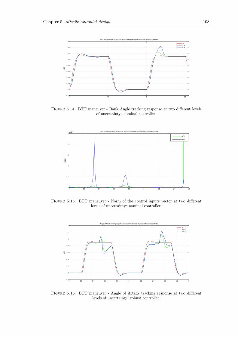
Chapter 5. Missile autopilot design 108
0 0.5 1 1.5−0.2
0
0.2
0.4
0.6
0.8
1
1.2
1.4
1.6Bank Angle regulation response at two different levels of uncertainty: nominal controller
t
φ(t)
ref30%60%
Figure 5.14: BTT maneuver - Bank Angle tracking response at two different levelsof uncertainty: nominal controller.
0 0.2 0.4 0.6 0.8 1 1.2 1.4 1.60
0.5
1
1.5
2
2.5x 10
4 Norm of the control inputs vector at two different levels of uncertainty: nominal controller
t
||u(t
)||
30%
60%
Figure 5.15: BTT maneuver - Norm of the control inputs vector at two differentlevels of uncertainty: nominal controller.
0 0.2 0.4 0.6 0.8 1 1.2 1.4 1.6 1.8 2−0.2
0
0.2
0.4
0.6
0.8
1
1.2
1.4Angle of Attack tracking response at two different levels of uncertainty: robust controller
t
α(t)
ref30%60%
Figure 5.16: BTT maneuver - Angle of Attack tracking response at two differentlevels of uncertainty: robust controller.
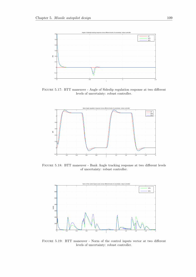
Chapter 5. Missile autopilot design 109
0 0.5 1 1.5−0.2
−0.1
0
0.1
0.2
0.3
0.4
0.5
0.6Angle of Sideslip tracking response at two different levels of uncertainty: robust controller
t
β(t)
ref
30%
60%
Figure 5.17: BTT maneuver - Angle of Sideslip regulation response at two differentlevels of uncertainty: robust controller.
0 0.2 0.4 0.6 0.8 1 1.2 1.4 1.6 1.8 2−0.2
0
0.2
0.4
0.6
0.8
1
1.2Bank Angle regulation response at two different levels of uncertainty: robust controller
t
φ(t)
ref30%60%
Figure 5.18: BTT maneuver - Bank Angle tracking response at two different levelsof uncertainty: robust controller.
0 0.2 0.4 0.6 0.8 1 1.2 1.4 1.6 1.8 20
100
200
300
400
500
600
700Norm of the control inputs vector at two different levels of uncertainty: robust controller
t
||u(t
)||
30%
60%
Figure 5.19: BTT maneuver - Norm of the control inputs vector at two differentlevels of uncertainty: robust controller.

Chapter 5. Missile autopilot design 110
maintain a better tracking along the whole reference trajectory even when uncertain
terms act in a more aggressive way (i.e. during agile BTT maneuvers).
0 0.5 1 1.50
0.2
0.4
0.6
0.8
1Norm of the tracking error vector at low uncertainty: comparison between nominal and robust controllers
t
||ex(t
)||
0 0.5 1 1.50
1
2
3
4x 10
4 Energy of the control inputs vector at low uncertainty: comparison between nominal and robust controllers
t
\int |
|u(t
)||^
2 \ d
t
nominal
robust
nominal
robust
Figure 5.20: BTT maneuver - Norm of the tracking error vector and energy of thecontrol inputs vector at low uncertainty: comparison between nominal and robust con-
trollers
0 0.5 1 1.50
0.2
0.4
0.6
0.8Norm of the tracking error vector at high uncertainty: comparison between nominal and robust controllers
t
||ex(t
)||
0 0.5 1 1.50
0.5
1
1.5
2
2.5
3x 10
4 Energy of the control inputs vector at high uncertainty: comparison between nominal and robust controllers
t
\int |
|u(t
)||^
2 \ d
t
nominal
robust
nominal
robust
Figure 5.21: BTT maneuver - Norm of the tracking error vector and energy of thecontrol inputs vector at high uncertainty: comparison between nominal and robust
controllers

Chapter 6
Immersion and Invariance under
sampling
The chapter is devoted to the implementation of the Immersion & Invariance stabiliza-
tion technique under sampling, when, i.e., the control input is maintained constant over
intervals of fixed length, namely the sampling period. This approach is not robust in
the sense that it counteracts the effects of model uncertainties and disturbances, as the
recursive Lyapunov redesign does. More precisely, the I&I technique adds robustness to
existing nonlinear controllers with respect to neglected dynamics, usually disregarded
because faster than the dominant dynamics or, in general, because considered less impor-
tant in control design. In several cases, such dynamics can critically affect the stability of
the closed-loop system, whereas the I&I approach is meant to preserve the desired prop-
erties exploiting, at least in part, the knowledge of the model of such dynamics. Often,
the presence of higher-order dynamics leads to time-scale separation designs, singular
perturbation and center manifold techniques to simplify the design. Such dynamics, for
instance associated to fast flexible motions or to actuator dynamics, usually neglected
at a first stage of the design, can be suitably handled in the I&I setting.
In this chapter, we reformulate in the sampled-data context the I&I stabilization paradigm
for a class of nonlinear systems in feedback form and we propose a constructive solution
based on the multi-rate control design philosophy. The main idea is to ensure, via a dig-
ital multi-rate construction, the matching of the closed-loop continuous-time evolution
of the function φ(x), describing implicitly the manifold, with the same trajectory under
digital control, at the sampling instants. The asymptotic dependency from the sampling
period of the multi-rate equivalent model allows for computable approximate solutions.
The sampled data design, by reproducing the behavior of φ at the sampling instants,
111

Chapter 6. Immersion and Invariance under sampling 112
directly guarantees manifold attractivity. Boundedness of the trajectories and the prop-
erties of system immersion and manifold invariance are preserved under sampling [93]
[90] [87]. The performance improvement of the proposed controllers relies in a remark-
able increase of the Maximum Allowable Sampling Period (MASP) with respect to the
direct implementation through zero-order hold of the continuous-time solution, which is
emulated control. The effectiveness of the proposed control strategy is evaluated on two
academic examples and a case study, the cart-pendulum system.
6.1 Sampled-data I&I control design
We consider the problem of I& I stabilization of systems of the form (3.54)-(3.53) and we
propose sampled-data solutions in terms of single-rate and multi-rate controllers, which
we apply to two academic examples. Next, we apply the digital single-rate solution to
the cart-pendulum system.
Problem setting Assume that the control input u is maintained piecewise constant
on intervals of fixed length, which is the sampling period. We look for a possibly
sampling-dependent controller, which maintains the stability properties achieved by the
continuous-time control law under sampling. In particular, the digital controller should
verify the sampled-data versions of conditions H1c-H4c of Theorem 3.4.0.11, achieving
manifold attractivity and keeping the boundedness of the trajectories under sampling.We
seek a sampled-data controller which, following the closed-loop continuous-time evolu-
tion of the function φ(x), ensures attractivity of M and boundedness under sampling.
The closed-loop system under digital control should be globally asymptotically stable.
To begin with, let us briefly recall the sampled-data equivalent dynamics under single
and multi-rate sampling.
6.1.1 Sampled-data equivalent models
The single-rate sampled-data equivalent model is the discrete-time dynamics reproducing,
at the sampling instants, the solution of (3.54) when the control variable u(t) is kept
constant over time periods of length δ, namely u(t+ τ) = u(t) = uk for 0 ≤ τ < δ, t =
kδ, k ≥ 0. It is described by the δ-parametrized map F δ(., uk) (the pair u, F δ) admitting
the Lie exponential series expansion:
xk+1 = F δ(xk, uk) = eδ(f+ukg)xk (6.1)

Chapter 6. Immersion and Invariance under sampling 113
On the other hand, the multi-rate sampled-data equivalent model of order m - MRm -
reproduces, at the sampling instants, the continuous-time behavior of (3.53) when u(t)
is maintained constant at values uik, over intervals of length δ = δm for τ ∈ ((i−1)δ, iδ).
Over each δ = mδ, it is described by the δ-parametrized map (the pair ui, Fmδ for
i = 1, . . .m)
xk+1 = Fmδ(xk, u1k, · · · , umk) (6.2)
= eδ(f+u1kg) ... eδ(f+umkg)xk
From the computational point of view, it is convenient to define the approximate versions
of these representations, namely the approximate single-rate ( resp. multi-rate) sampled-
data model of degree ν, with reference to truncations of the expansions (6.1) (resp. (6.2))
at finite order ν in δ, i.e.
F δ(x, u) = F δ[ν](x, u) +O(δν) (6.3)
Fmδ(x, u1, ..., um) = Fmδ[ν](x, u1, ..., um) +O(δν) (6.4)
Remark 6.1.1.1. With ν = 1 (approximation in O(δ2)), one recovers the well known Eu-
ler sampled-data dynamics xk+1∼= xk + δf(xk) + δukg(xk), preserving the structure of the
continuous-time system. ♦
6.1.2 Main result
The sampled-data control is designed employing a multi-rate strategy (see [92]) of order
n − p, which achieves manifold attractivity under sampling by matching the evolu-
tion of φ(x), under continuous-time control (3.59), at the sampling instants. Since the
continuous-time assumptions are fulfilled, we expect φ to vanish asymptotically. Bound-
edness under sampling is ensured by matching between the sampled-data trajectory and
the continuous-time one. The behavior on the manifold is reduced to that of the target
system under sampling, yielding the global asymptotic stability of the digital control
system.

Chapter 6. Immersion and Invariance under sampling 114
Theorem 6.1.2.1. Consider the class of feedback systems (3.53) satisfying assumptions 3.4.2.1
and 3.4.2.2, with n− p = 2, with an equilibrium x∗ to be stabilized. There exists an order m = 2
multi-rate sampled-data control law of the form
ud1 = ψδ1(xk, φ(xk))
ud2 = ψδ2(xk, φ(xk))(6.5)
such that x∗ is a globally asymptotically stable equilibrium of the closed-loop dynamics
xk+1 = F 2δ(xk, ψδ1(xk, φ(xk)), ψδ2(xk, φ(xk))) (6.6)
♦
Proof. Following assumptions H1c to H4c of the continuous-time result, we can define
for (3.53) a sampled-data equivalent target system, with state ξ ∈ Rp
ξk+1 = αd(ξk) (6.7)
where αd(ξ) = eδf1(ξ,0)ξ has a globally asymptotically stable equilibrium at ξ∗ ∈ Rp and
x∗ = π(ξ∗). Condition H2c can be reformulated as follows
F 2δ(π(ξk), 0) = π(αd(ξk)) (6.8)
which, exploiting the properties of the exponential representation, yields that π is equal
to the identity function for the first p components, while it is necessarily equal to zero
for the remaining n− p components. Thus invariance under sampling is ensured. Keep
in mind that, for the class of systems at study, c(ξ) = 0. As a consequence, the implicit
manifold condition H3c is verified under sampling with the choice φ1(x) = x2, φ2(x) =
x3. The existence of a multi-rate controller of the form (6.5) for (3.53) is ensured
provided the following rank condition [93] is fulfilled
rank[g, adfg, ad2fg, . . . , adpfg, . . .] ≥ n− p. (6.9)
When applied to (3.53), condition (6.9) results verified if ∂f2∂x36= 0, which is true thanks to
the assumptions 3.4.2.1 and 3.4.2.2. Consider now the extended system under sampling
(i = 1, 2)
zk+1 = φ(F (n−p)δ(xk, ψδi (xk, zk)) (6.10)
xk+1 = F (n−p)δ(xk, ψδi (xk, zk)) (6.11)

Chapter 6. Immersion and Invariance under sampling 115
where z = φ(x) = (xn−1, xn)T . Attractivity ofM is ensured by matching the continuous-
time trajectories of φ(x), which for the systems under study reduces to a simple input
to partial-state matching, achieved by the existing multi-rate solution according to the
results in [93]. As a consequence, limk→∞ zk = 0. Boundedness of the trajectories of
(6.10) is guaranteed by one-step consistency property plus forward completeness of the
vector fields of (3.53), hence the thesis.
Remark 6.1.2.2. In general, with x2 of dimension q, the sampled-data I&I solution is given
by a multi-rate control law of order m = q + 1. The multi-rate controller is built to follow the
closed-loop continuous-time evolution of the function φ(x). ♦
In the following, we are going to develop an approximate version of the proposed digital
controller (6.5), leading to a computable control law.
6.1.3 Sampled-data approximate design
We derived the continuous-time I&I stabilizing control law (3.59) for a special class of
systems in the case n− p > 1, establishing that a sampled-data multi-rate control logic
is well suited to solve the problem in a digital setting. Now we look for constructive,
approximate, solutions according to (6.3).
6.1.3.1 Single-rate solution
For the class of systems (3.54), with n − p = 1, the continuous-time solution (3.55),
namely γ(x), yields a single-rate sampled-data controller ud designed to match at the
sampling instants the controlled x2 dynamics. The matching condition is
eδf(.,ud)x2 = eδf(.,γ)φ|x1,x2 (6.12)
with f(x1, x2, u) = f1(x1, x2) ∂∂x1
+u ∂∂x2
. In this case, since x2 = u, (6.12) is satisfied by
the single-rate sampled-data control law
ud = γ(x) +δ
2!γ(x) +
δ2
3!γ(x) +
∑i≥3
δi
(i+ 1)!u(i)c (x) (6.13)

Chapter 6. Immersion and Invariance under sampling 116
According to (6.3), an approximate version of (6.13), truncated at the first term in
O(δ2), can be given as follows:
ud = ud0 +δ
2ud1. (6.14)
Note that the term ud0 = γ(x)|xk is the emulated controller, with xk = x(t = kδ) and
ud1 = uc(x)|xk = ∂γ∂x(f + gγ(x))|xk .
In this particular case, the digital control can be directly expressed in terms of the
continuous-time control input as follows:
ud =1
δ
∫ (k+1)δ
kδuc(τ)d τ, (6.15)
which is exactly the average of the continuous control signal evaluated on the sampling
period.
6.1.3.2 Multi-rate solution
For systems in the form (3.53), the multi-rate solution is better suited as well as of
straightforward derivation. In the case n− p = 2, a multi-rate controller of order m = 2
can be designed to match the continuous-time controlled trajectories of φ(x) = (x2, x3)T
at the sampling instants. Recall that the continuous-time solution (3.59) is of the form
ψ(x1, φ(x)). The input to partial-state matching conditions in this case are given by
eδ(f+ud1g) eδ(f+ud2g)x2 = eδ(f+ψ(·,·)g)φ1|x1,z
eδ(f+ud1g) eδ(f+ud2g)x3 = eδ(f+ψ(·,·)g)φ2|x1,z(6.16)
where f = (f2(x2, x3), 0)T , g = (0, 1)T . As stated by Theorem 6.1.2.1, there exists a
multi-rate sampled-data control law of order 2, satisfying (6.16), of the form
ud1 = ud10 +∑i≥1
δi
(i+ 1)!ud1i over [0, δ)
ud2 = ud20 +∑i≥1
δi
(i+ 1)!ud2i over (δ, δ]
(6.17)
The approximate control laws which solve the problem up to an error in O(δ3) (in x3),
arresting the expansions (6.17) at i = 2, are given by the following expressions for the
udji terms
ud10 = ud20 = ψ(x1, z)
ud11 =2
3uc1 ud21 =
10
3uc1
(6.18)

Chapter 6. Immersion and Invariance under sampling 117
where uc1 = ψ(x). Substituting (6.18) into (6.17) yields
ud1 = ψ(x) +δ
3ψ(x) ud2 = ψ(x) +
5δ
3ψ(x) (6.19)
with δ = 2δ. On the first sub-interval [0, δ) the control applied is ud1, which switches
to ud2 in [δ, δ). The obtained multi-rate control law (6.19) renders the origin of (3.59)
GAS under sampling, if δ is chosen small enough. The approximate single and multi-
rate controllers (6.14)-(6.19) overcome in performance the emulated control laws ud0 =
ud10 = ud20, preserving stability for increasing values of δ as shown in the two examples
below.
6.2 Example with single-rate control
The results can be illustrated through an academic example discussed in [6]
x1 = −x1 + x31x2
x2 = u(6.20)
with x1 and x2 ∈ R. In this particular case, z = φ(x) = x2 and, on the manifold,
uc = −(2 + x8
1
)x2|x2=0 = 0. Exploiting the arguments presented in [6], the continuous-
time stabilizing I&I control law is found to be
uc = −(2 + x8
1
)x2. (6.21)
The computation of the sampled feedback is made according to the approximate sampled-
data controller (6.14) which, truncated at the first term in O(δ), gives
ud = −(2 + x81)x2 +
δ
2x2
(x1
16− 8x2x110 + 12x8
1 + 4)
(6.22)
We compare the target system and the continuous-time trajectories with those under
emulated control ud0 and those under ud, for increasing values of the sampling period
δ. In the first scenario, with δ = 0.01 s, both controllers behaves very well and the
difference in performance is imperceptible. In the second scenario, with δ = 0.2 s, the
state trajectories under ud0 and ud track the target dynamics and the continuous time
evolution very well, with a slightly increased performance under ud (Fig. 6.1, 6.2, 6.3).
In the third scenario, with δ = 0.8 s, the state trajectories convergence under ud is
still more than acceptable: boundedness and attractivity are preserved. However, as
expected, the behavior under ud0 is unstable as shown in Fig. 6.4, 6.5 and 6.6.

Chapter 6. Immersion and Invariance under sampling 118
0 0.5 1 1.5 2 2.5 3 3.5 4 4.5 50
0.2
0.4
0.6
0.8
1
1.2
1.4
1.6
1.8
2
Figure 6.1: x1 evolutions and comparison with the target system when δ = 0.2 s.In black the target system, in red the continuous-time evolution, in blue the evolution
under ud and in green that under ud0.
0 0.5 1 1.5 2 2.5 30
0.2
0.4
0.6
0.8
1
1.2
1.4
1.6
1.8
2
Figure 6.2: x2 evolutions when δ = 0.2 s. In red the continuous-time evolution, inblue the evolution under ud and in green that under ud0.
0 0.5 1 1.5 2 2.5−7
−6
−5
−4
−3
−2
−1
0
1
Figure 6.3: u when δ = 0.2 s. In red the continuous-time input, in blue ud and ingreen ud0.

Chapter 6. Immersion and Invariance under sampling 119
0 0.5 1 1.5 2 2.5 3 3.5 4−1
−0.5
0
0.5
1
1.5
2
Figure 6.4: x1 evolutions and comparison with the target system when δ = 0.8 s.In black the target system, in red the continuous-time evolution, in blue the evolution
under ud and in green that under ud0.
0 1 2 3 4 5 6 7 8−3
−2
−1
0
1
2
3
4
5
Figure 6.5: x2 evolutions when δ = 0.8 s. In red the continuous-time evolution, inblue the evolution under ud and in green that under ud0.
0 1 2 3 4 5 6 7 8−10
−8
−6
−4
−2
0
2
Figure 6.6: u when δ = 0.8 s. In red the continuous-time input, in blue ud and ingreen ud0.

Chapter 6. Immersion and Invariance under sampling 120
6.3 Example with multi-rate control
Let us consider the nonlinear system
x1 = −x1 + x21x
22
x2 = x22 + x3
x3 = u
(6.23)
which is a system of the form (3.58) with target dynamics ξ = −ξ, α(·) : R → R. In
this case p = 1, hence n − p = 2. Due to the lower-triangular structure of the system,
conditions H2c and H3c hold with c(ξ) = 0 and z = φ(x) = (x2, x3)T . Manifold
attractivity and boundedness of the trajectories are achieved using simple nonlinear
domination arguments, thus applying (3.59) with the choice k1 = 2 + x41, k2 > 0, results
in the control law:
u = −x2 −(2x2 + 2 + x4
1
) (x3 + x2
2
)− 4x2x
31
(−x1 + x2
1x22
)− k2
(x3 + x2
2 + 2x2 + x2x41
) (6.24)
which ensures limz→∞ = 0 and boundedness of the trajectories choosing
W =1
2x2
1 +1
2
(x2
2 +(x3 + x2
2 + 2x2 + x2x41
)2)(6.25)
Remark 6.3.0.1. The Lyapunov function (6.25) represents a quite strong choice. In fact, it
is possible to relax the choice of V , using a weak Lyapunov function, with derivative negative
outside a compact set containing the origin, or even a semidefinite Lyapunov function: the
boundedness property required for x1 is still maintained. Other issues, as reducing the dimensions
of the (ultimate) bound or the time of convergence, can be taken into account exploiting further
design parameters. ♦
The sampled-data design aims at following the closed-loop behavior of the two-dimensional
function φ = (x2, x3)T with a multi-rate controller of order two. The classical solutions
with m = n − p = 2 are truncated at the first order in δ, so we apply (6.19) directly.

Chapter 6. Immersion and Invariance under sampling 121
Setting k2 = 4, the expression of uc1 takes the form
uc1 = 4x91x
32 + x8
1x22 + x8
1x3 − 20x61x
52 − 8x5
1x42 + 44x5
1x32
− 16x51x
22x3 + 2x4
1x32 + 16x4
1x22 + 2x4
1x2x3
+ 9x41x2 + 16x4
1x3 − 2x42 + 12x3
2 − 4x22x3
+ 45x22 + 12x2x3 + 54x2 − 2x2
3 + 27x3.
(6.26)
Note that the multi-rate solution combines the emulation of the continuous controller
with its weighted derivative in closed-loop. Again, we compare the target system and
the continuous-time trajectories with those under emulated control ud10−ud20 and those
under ud1 − ud2, for increasing values of the sampling period δ.
In the first scenario, with δ = 0.05 s, both the emulated and the multi-rate solutions
behave well in steering to zero system trajectories (Fig. 6.7, 6.8). However, a nervous
transient behavior can be observed in the emulated case, especially in the control input
(Fig. 6.9). In the second scenario, with δ = 0.1 s, it is clear from Fig. 6.10, 6.11 and
0 0.5 1 1.5 2 2.5 3 3.5 4 4.5 50
0.2
0.4
0.6
0.8
1
1.2
1.4
1.6
1.8
2
t
x 1(k)
Figure 6.7: x1 evolutions and comparison with the target system when δ = 0.05 s.In black the target system, in red the continuous-time evolution, in blue the evolution
under multi-rate and in green that under ud10 − ud20.
6.12 that the emulated controller cannot guarantee stability anymore, while the behavior
under multi-rate control is still more than acceptable.
Next, we propose the application of the single-rate digital controller to an underactuated
system with relative degree one, the cart-pendulum. Also in this case, the continuous-
time solution has been studied and proposed in [5].

Chapter 6. Immersion and Invariance under sampling 122
0 0.2 0.4 0.6 0.8 1 1.2 1.4 1.6 1.8 20
0.5
1
1.5
2
2.5
x 2(k)
0 0.2 0.4 0.6 0.8 1 1.2 1.4 1.6 1.8 2−25
−20
−15
−10
−5
0
5
t
x 3(k)
Figure 6.8: x2 and x3 evolutions when δ = 0.05 s. In red the continuous-timeevolution, in blue the evolution under multi-rate and in green that under ud10 − ud20.
0 0.1 0.2 0.3 0.4 0.5 0.6 0.7 0.8 0.9 1−200
−150
−100
−50
0
50
100
150
200
250
300
Figure 6.9: u when δ = 0.05 s. In red the continuous-time input, in blue the multi-rateand in green the emulated.
0 0.5 1 1.5 2 2.5 3 3.5 40
2
4
6
8
10
12
14
t
x 1(k)
Figure 6.10: x1 evolutions and comparison with the target system when δ = 0.1 s.In black the target system, in red the continuous-time evolution, in blue the evolution
under multi-rate and in green that under ud10 − ud20.

Chapter 6. Immersion and Invariance under sampling 123
0 0.2 0.4 0.6 0.8 1 1.2 1.4 1.6−2
0
2
4
6
8
10
x 2(k)
0 0.1 0.2 0.3 0.4 0.5 0.6 0.7 0.8 0.9 1−40
−20
0
20
40
60
80
100
120
t
x 3(k)
Figure 6.11: x2 and x3 evolutions when = δ = 0.1 s. In red the continuous-timeevolution, in blue the evolution under multi-rate and in green that under ud10 − ud20.
0 0.5 1 1.5−200
−150
−100
−50
0
50
100
150
Figure 6.12: u when δ = 0.1 s. In red the continuous-time input, in blue the multi-rate and in green the emulated.
6.4 The cart-pendulum system
Following [6], we develop a sampled-data controller for a classical example based on
an underactuated system with three state variables, the cart-pendulum. The partially-
linearized and normalized cart-pendulum system equations of motion are
x1 = x2
x2 = sin(x1)− u cos(x1)
x3 = u
(6.27)
where (x1, x2) ∈ S1 × R are the pendulum angle (w.r.t. the upright vertical) and its
velocity, x3 ∈ R is the velocity of the cart and u ∈ R is the control input. We want to
stabilize the pendulum in its upward position, with the cart stopped, corresponding to

Chapter 6. Immersion and Invariance under sampling 124
the equilibrium x∗ = 0. Usually, a smart target-system choice for this kind of systems is
the unactuated part of the mechanism to which has been assigned a desired dynamics,
in this case that of a fully actuated pendulum
ξ1 = ξ2
ξ2 = −V ′(ξ1)−R(ξ1, ξ2)ξ2
(6.28)
with R(·) damping function, R(0, 0) > 0, V (ξ1) potential energy function, V ′(0) = 0
and V ′′(0) > 0, and H(ξ1, ξ2) = 12ξ
22 + V (ξ1) total energy function. A natural selection
of the mapping π(·) is
π(ξ) =
ξ1
ξ2
π3(ξ1, ξ2)
(6.29)
The choice π3(x1, x2) = −k1x1 − k2cos(x1)x2 with k1 > 0 and k2 > 1 yields the following
continuous-time control law
u(x) =1
k2 − 1
[γ
(x3 + k1x1 +
k2
cos(x1)x2
)+ k1x2 + k2 tan(x1)
(x2
2
cos(x1)+ 1
)] (6.30)
which, with γ > 0, solves the problem of I&I stabilization of the origin of the cart-
pendulum system. For a detailed discussion of the continuous-time control design, see
[6] and the references therein.
Since the relative degree of (6.27), considering x1 as output function, is one, the compu-
tation of the sampled feedback can be done according to (6.13), which for the first term
in O(δ2) gives
u(x) =
(g
(k1 + k2x2 sin(x1)
cos(x1)2+ k2 tan(x1)2 + 1
)(x22
cos(x1)+ 1
)+k2x
22 sin(x1) tan(x1)
cos(x1)2(k2 − 1)
)x2 +
(k1 +
gk2cos(x1)
+2k2x2
tan(x1) cos(x1)(k2 − 1)
)× (sin(x1) − cos(x1)u(x)) +
g
(k2 − 1)u(x)
(6.31)
Simulations are carried out to highlight the difference in performance between the em-
ulated controller, which is (6.30) evaluated at the sampling instants t = kδ, and the
digital controller with the first order corrector term defined in (6.31). Two scenarios are
considered: the first with sampling time T = 0.1 s and the second with T = 0.3 s.
When the sampling time is sufficiently small, as in the case of T = 0.1 s, both the
emulated and the first-order controllers behave well in reaching asymptotically the target
system evolution, as shown in Fig. 6.13, 6.14, 6.15. The continuous-time trajectories are

Chapter 6. Immersion and Invariance under sampling 125
well followed by both the controllers. However, note that the transient response shown
by the system controlled using the first-order correction term is smoother and shows
less overshoot than the emulated response. Similar observations can be made for the
control inputs transient responses in Fig. 6.16. The superiority of the controller with
correction term is mostly due to the predictive action of u, which increases damping. In
the following figures we show in black the target system evolution, in red the continuous-
time one, in green the evolution under emulation of the continuous-time controller and
in blue the state trajectories of the system in closed-loop with the first order correction
controller.
0 2 4 6 8 10 12 14 16 18−1.5
−1
−0.5
0
0.5
1
1.5
Figure 6.13: Pendulum heading angle w.r.t. the vertical, comparison between con-tinuous (red) and sampled-data controllers (emulated in green and first order in blue)
at T = 0.1 s
0 2 4 6 8 10 12−5
−4
−3
−2
−1
0
1
2
Figure 6.14: Pendulum angular velocity, comparison between continuous (red) andsampled-data controllers (emulated in green and first order in blue) at T = 0.1 s
In the second scenario, the sampling time is increased at the value of T = 0.3 s. This
seems to be a critical value for the system, since the emulated controller doesn’t work
anymore, while the first-order corrected controller is still able to follow the target system
behavior, as shown in Fig. 6.17, 6.18, 6.19, 6.20.

Chapter 6. Immersion and Invariance under sampling 126
0 1 2 3 4 5 6 7 8 9 10
−5
0
5
10
15
Figure 6.15: Cart velocity trajectory, comparison between continuous (red) andsampled-data controllers (emulated in green and first order in blue) at T = 0.1 s
0 1 2 3 4 5 6 7 8 9 10−20
−15
−10
−5
0
5
10
15
20
Figure 6.16: Control input, comparison between continuous (red) and sampled-datacontrollers (emulated in green and first order in blue) at T = 0.1 s
0 2 4 6 8 10 12−2
−1.5
−1
−0.5
0
0.5
1
1.5
2
Figure 6.17: Pendulum heading angle w.r.t. the vertical, comparison between con-tinuous (red) and sampled-data controllers (emulated in green and first order in blue)
at T = 0.3 s

Chapter 6. Immersion and Invariance under sampling 127
0 2 4 6 8 10 12
−20
−15
−10
−5
0
5
10
15
Figure 6.18: Pendulum angular velocity, comparison between continuous (red) andsampled-data controllers (emulated in green and first order in blue) at T = 0.3 s
0 2 4 6 8 10 12−5
0
5
10
15
20
Figure 6.19: Cart velocity trajectory, comparison between continuous (red) andsampled-data controllers (emulated in green and first order in blue) at T = 0.3 s
0 1 2 3 4 5 6 7 8 9−30
−25
−20
−15
−10
−5
0
5
10
15
20
Figure 6.20: Control input, comparison between continuous (red) and sampled-datacontrollers (emulated in green and first order in blue) at T = 0.3 s
Chapter 7
Robust attitude stabilization via
digital I&I
In this chapter, we face the problem of robust nonlinear attitude stabilization of a
rigid spacecraft. An Immersion and Invariance robust attitude stabilizer is proposed,
taking into account actuator dynamics in control design. The proposed continuous-
time controller is then implemented under sampling using an approximated single-rate
strategy to match, at the sampling instants, the zero-going evolution of the off-the-
manifold coordinates. The results illustrated in section 6.1 for the single-rate solution
are easily extended to the case of more than one control input. Simulations show the
effectiveness of the proposed controller. The chapter follows the paper [88] submitted
to the first MICNON conference and waiting for review.
7.1 Introduction
A nonlinear control strategy to stabilize the attitude of a rigid spacecraft robustly with
respect to actuators dynamics is proposed. The control law is applied under sampling
using a single-rate digital approach with first order corrector term, which overcomes in
performance the direct implementation through zero-order hold, as shown by simula-
tions. A robust attitude stabilizer is necessary for long range communications satellites,
especially when a high throughput is involved. The capability of the spacecraft to
maintain a fixed orientation despite external disturbances and modeling uncertainties
is crucial when dealing with satellite internet access at high data speeds [101]. In this
work we propose an I&I solution for systems in strict-feedback form which is particu-
larly suited to counteract the degrading effect of unmodeled actuator dynamics on the
overall control systems. In fact, I&I can be regarded as a tool to robustify a given
128

Chapter 7. Robust attitude stabilization via I&I 129
nonlinear controller with respect to higher-order dynamics, exploiting at its best the
knowledge of such dynamics during the control design phase. Thus, this approach can
be considered “robust” nonlinear control. The obtained continuous-time controller is
then implemented under sampling using a single-rate control strategy with truncation
of series expansions at the second order in the sampling period. Simulations at increasing
sampling times show the effectiveness of using a first order corrector term with respect
to the simpler implementation through zero-order hold device (emulated control [97]).
In particular, the maximum allowable sampling period (MASP) is increased, thus the
sampled-data controller shows robustness w.r.t. δ.
7.2 Spacecraft dynamic modeling
Consider a symmetric rigid spacecraft characterized by a diagonal inertia matrix J ,
namely
J =
Jx 0 0
0 Jy 0
0 0 Jz
.
The kinematic model used is based on the modified Cayley-Rodrigues parameters, which
provide a global and non-redundant parametrization of the attitude of a rigid body ([26]).
In the following, S(·) denotes the three-dimensional skew-symmetric matrix, which for
a generic vector r ∈ R3 takes the form
S(r) =
0 r3 −r2
−r3 0 r1
r2 −r1 0
(7.1)
Defining ρ ∈ R3 the modified Cayley-Rodrigues parameters vector and ω ∈ R3 the
angular velocity in a body-fixed frame, the kinematic equations take the form
ρ = H(ρ)ω. (7.2)
The matrix-valued function H : R3 → R3×3 denotes the kinematic jacobian matrix of
the modified Cayley-Rodrigues parameters, given by
H(ρ) =1
2
(I − S(ρ) + ρρT − 1 + ρTρ
2I
)(7.3)
Chapter 7. Robust attitude stabilization via I&I 130
where I denotes the 3 × 3 identity matrix. The matrix H(ρ) satisfies the following
identity ([127])
ρTH(ρ)ω =
(1 + ρTρ
4
)ρTω (7.4)
for all ρ, ω ∈ R3.
According to Euler’s law, the kinematic and dynamic equations can be written as
ρ = H(ρ)ω (7.5)
ω = J−1S(ω)Jω + J−1u. (7.6)
If first-order actuator dynamics with time-constants Ti (i = 1, 2, 3) are considered, equa-
tions (7.5)-(7.6) are dynamically extended as follows
ρ = H(ρ)ω (7.7)
ω = J−1S(ω)Jω + J−1τ (7.8)
τ = Aτ + u. (7.9)
where τ ∈ R3 represents the torque generated by the actuators according to the refer-
ence torque u ∈ R3 and A = diag(− 1T1,− 1
T2,− 1
T3) is a Hurwitz diagonal matrix whose
eigenvalues, all negative real, depend on the time constants of the actuators.
7.3 Immersion and Invariance stabilization
7.3.1 Recalls
Let us recall the continuous-time I&I main result in the general case (the proof is detailed
in [5]).
Theorem 7.3.1.1. Consider the nonlinear system
x = f(x) + g(x)u (7.10)
with state x ∈ Rn, control input u ∈ Rm and an equilibrium point x∗ ∈ Rn to be stabilized.
Suppose that (7.10) satisfies the following four conditions.
H1c (Target System) - There exist maps α(·) : Rp → Rp and π(·) : Rp → Rn such that the sub-
system ξ = α(ξ) with state ξ ∈ Rp, p < n, has a (globally) asymptotically stable equilibrium
at ξ∗ ∈ Rp and x∗ = π(ξ∗).

Chapter 7. Robust attitude stabilization via I&I 131
H2c (Immersion condition) - For all ξ ∈ Rp, there exists a map c(·) : Rp → Rm such that
f(π(ξ)) + g(π(ξ))c(ξ) =∂π
∂ξ(ξ)α(ξ) (7.11)
H3c (Implicit manifold - M) - There exists a map φ(·) : Rn → Rn−p such that the identity
between sets x ∈ Rn|φ(x) = 0 = x ∈ Rn|x = π(ξ) for ξ ∈ Rp holds.
H4c (Manifold attractivity and trajectory boundedness) - There exists a map ψ(·, ·) : Rn×(n−p) →Rm such that all the trajectories of the system, with initial condition z0 = φ(x0)
z =∂φ
∂x[f(x) + g(x)ψ(x, z)] (7.12a)
x = f(x) + g(x)ψ(x, z) (7.12b)
are bounded and satisfy limt→∞ z(t) = 0.
Under these four conditions, x∗ is a globally asymptotically stable equilibrium of the closed-loop
system
x = f(x) + g(x)ψ(x, φ(x)) (7.13)
♦
The following definition is straightforward.
Definition 7.3.1.2 (I&I Stabilizability). A nonlinear system of the form (7.10) is said to be
I&I stabilizable with target dynamics ξ = α(ξ), if it satisfies conditions H1c to H4c of Theorem
7.3.1.1. ♦
Note that the target dynamics is the restriction of the closed-loop system to the manifold
M, implicitly defined in H3c. The control law u = ψ(x, z) is designed to steer to zero the
off-the-manifold coordinate z and to guarantee the boundedness of system trajectories.
On the manifold, the control law is reduced to ψ(π(ξ), 0) = c(ξ), and it renders Minvariant according to H2c. The complete control law can thus be decomposed in two
parts:
u = ψ(x, φ(x)) = ψ(x, 0) + ψ(x, φ(x)) (7.14)
with ψ(π(ξ), 0) = c(ξ) on the manifold and ψ(x, 0) = 0. Note that ψ(x, 0) can be seen as
a nominal control law, designed on the model of the dynamics restricted on the manifold
to obtain a GAS target dynamics. In this sense, the term ψ(x, φ(x)) is a robustness-
improving addendum which takes into account the off-the-manifold behaviors generated,
for instance, by higher-order actuator dynamics. The overall control law provides the
I&I “robust” nonlinear stabilizer.

Chapter 7. Robust attitude stabilization via I&I 132
7.3.2 The class of systems under study
In this work, we consider the problem of state-feedback stabilization of the following
class of systems in feedback form
ξ = f(ξ) + g(ξ)η
η = u(7.15)
where ξ ∈ Rp, η ∈ Rn−p, u ∈ Rm (with m = n− p), x = col(ξ, η) and ξ = 0 is a globally
asymptotically stable equilibrium of ξ = f(ξ). It is also assumed that we know a radially
unbounded Lyapunov function V (ξ) such that
∂V
∂ξf(ξ) < −w(‖ξ‖) (7.16)
with w(·) K∞ function. Note that the existence of V is guaranteed by the converse
Lyapunov theorems, although in many cases its knowledge or construction could be
difficult to achieve. For systems like (7.15) constructive solutions of the I&I stabilization
problem do exist, as shown with more detail in [5]. In fact, the target dynamics condition
H1c is trivially satisfied by ξ = f(ξ). Moreover, the mappings
x =
[π1(ξ)
π2(ξ)
]=
[ξ
0
]u = c(ξ) = 0 φ(ξ, η) = η (7.17)
are such that conditions H2c and H3c hold. Since the off-the-manifold component z = η
is a partial-coordinate, condition H4c is verified if it is possible to find a control law
u = ψ(ξ, η) such that the trajectories of the closed-loop system
ξ = f(ξ) + g(ξ)η
η = ψ(ξ, η)(7.18)
are bounded and limt→∞ η(t) = 0 (manifold attractivity). To this end, it is possible to
relax the assumption on V to be a weak Lyapunov function, namely such that (7.16)
holds for all ‖ξ‖ > M > 0, for a proper, problem-dependent, choice of M (see [5] for
more details). With this in mind, we can state the following result.
Theorem 7.3.2.1. Consider system (7.18) with all the related properties and assumptions. The
system satisfies condition H4c, i.e. manifold attractivity and trajectory boundedness, with the

Chapter 7. Robust attitude stabilization via I&I 133
following choice for the control law:
ψ(ξ, η) = −(µ(ξ) + kη)η
µ(ξ) >
∥∥∥∥∂V∂ξ g(ξ)
∥∥∥∥ kη > 0.(7.19)
♦
Proof. Substituting (7.19) into (7.18) yields
ξ = f(ξ) + g(ξ)η
η = −(µ(ξ) + kη)η.(7.20)
Consider now the Lyapunov function
W (ξ, η) = V (ξ) +1
2ηT η. (7.21)
The derivative of (7.21) along the trajectories of (7.20) takes the form
W =∂V
∂ξf(ξ) +
∂V
∂ξg(ξ)η − µ(ξ)ηT η − kηηT η
≤ −w(‖ξ‖) +
∥∥∥∥∂V∂ξ g(ξ)
∥∥∥∥ ‖η‖2 − µ(ξ) ‖η‖2 − kη ‖η‖2
≤ −w(‖ξ‖) +
(∥∥∥∥∂V∂ξ g(ξ)
∥∥∥∥− µ(ξ)
)‖η‖2 − kη ‖η‖2
≤ −w(‖ξ‖)− kη ‖η‖2
(7.22)
which is negative definite for all ‖ξ‖ > M > 0 thanks to the proper choice of µ(ξ) and
kη, thus condition H4c is verified, which concludes the proof.
7.3.3 Problem setting
Assume now that the control input u is maintained piecewise constant on intervals of
fixed length, namely the sampling period. We seek a possibly sampling-dependent con-
troller, which maintains the stability properties achieved by the continuous-time control
law under sampling. In particular, the digital controller should verify the sampled-data
versions of conditions H1c-H4c of Theorem 3.4.0.11, achieving manifold attractivity and
keeping the boundedness of the trajectories under sampling.

Chapter 7. Robust attitude stabilization via I&I 134
7.4 Sampled-data control design
We seek a sampled-data controller which, following the closed-loop continuous-time evo-
lution of the function φ(ξ, η) = η, ensures attractivity of the manifold M and bound-
edness of the closed-loop trajectories under sampling. The closed-loop system under
digital control should be globally asymptotically stable. To begin with, let us briefly
recall the sampled-data equivalent dynamics under single-rate sampling. In order to
simplify the problem and to fit it to that of attitude stabilization of the rigid spacecraft,
the following two assumptions are straightforward.
Assumption 7.4.0.1. Consider system (7.15). With the aim of designing the sampled-
data controller, it is assumed that the dimension of the vector ξ is equal to that of η
and u, namely p = m, thus n = 2m. As a consequence, the matrix g(ξ) is squared,
g(x) ∈ Rm×m. ♦
Assumption 7.4.0.2. Consider system (7.15). For the sake of simplicity of the sampled-
data control design it is assumed that the matrix g(ξ) is diagonal and does not depend
on ξ, namely g(ξ) = G. Moreover, it is assumed that it is non-singular, i.e. detG 6= 0.♦
Next, let us rewrite system (7.15) in the following form (i = 1, . . . ,m):
xi = fi(x) + uig (7.23)
where xi = col(ξi, ηi), ui is the ith component of the control input, fi(x) = col(fi(ξ) +
Giηi, 0), Gi is the ith row-ith column element of G and g = col(0, 1). In this way, the
n-dimensional multi-input system is decomposed into m single-input systems, each of
dimension two.
The single-rate sampled-data equivalent model is the discrete-time dynamics reproducing,
at the sampling instants, the solution of (7.23) when the control variable ui(t) is kept
constant over time periods of length δ, namely ui(t + τ) = ui(t) = uik for 0 ≤ τ <
δ, t = kδ, k ≥ 0. It is described by the δ-parametrized map F δi (., uik) (the pair ui, Fδi )
admitting the Lie exponential series expansion:
xi(k+1) = F δi (xik, uik) = eδ(fi+uik g)xik (7.24)
The sampled-data control is designed employing a single-rate strategy (see [92]), which
achieves manifold attractivity under sampling by matching the controlled continuous-
time evolution of φ = η at the sampling instants. Since the continuous-time conditions
are fulfilled by (7.19), φ will vanish asymptotically. A digital control law reproducing
the φ behavior is proposed to steer system trajectories on the manifold. The behavior on

Chapter 7. Robust attitude stabilization via I&I 135
the manifold is reduced, by construction, to that of the target system under sampling,
yielding global asymptotic stability of the digital control system.
Theorem 7.4.0.3. Consider the class of feedback systems (7.15) satisfying assumptions 7.4.0.1
and 7.4.0.2 with an equilibrium x∗ to be stabilized. Moreover, consider the stabilizing continuous-
time control law (7.19), ψ(ξ, η) ∈ Rm. There exist sampled-data control laws of the form (i =
1, . . . ,m)
udi = ψδi (ξk, ηk) (7.25)
such that x∗ is a globally asymptotically stable equilibrium of the closed-loop dynamics (i =
1, . . . ,m)
xi(k+1) = F δi (xik, ψδi (ξk, ηk)) (7.26)
♦
Proof. Following assumptions H1c to H4c of the continuous-time result, we can define
for (7.15) a sampled-data equivalent target system, with state ξ ∈ Rp
ξk+1 = fd(ξk) (7.27)
where fd(ξ) = eδf(ξ)ξ has a globally asymptotically stable equilibrium at ξ∗ ∈ Rp and
x∗ = π(ξ∗). Condition H2c can be reformulated as follows, for i = 1, . . . ,m,
F δ(π(ξk), 0) = π(fd(ξk)) (7.28)
which, exploiting the properties of the exponential representation, yields that π is equal
to the identity function for the first p components, while it is necessarily equal to zero
for the remaining n − p = m components. Thus invariance under sampling is ensured.
Keep in mind that, for the class of systems at study, c(ξ) = 0. As a consequence,
the implicit manifold condition H3c is verified under sampling with the choice φ1(x) =
xp+1, φ2(x) = xp+2, . . . , φn−p(x) = xn or, alternatively, φ(x) = η. The existence of a
single-rate controller of the form (7.25) for (7.15) is ensured provided a controllability-
like condition [93] is fulfilled. For systems in strict-feedback form like (7.15) satisfying
assumption 7.4.0.1, such condition translates in requiring that det g(ξ) 6= 0, which is
automatically ensured by assumption 7.4.0.2, thus the sampled-data control law exists.
Consider now the extended system under sampling (i = 1, . . . ,m)
zi(k+1) = φ(F δi (xik, ψδi (ξk, ηk)) (7.29)
xi(k+1) = F δi (xik, ψδi (ξk, ηk)) (7.30)

Chapter 7. Robust attitude stabilization via I&I 136
Attractivity of M is ensured by matching the continuous-time trajectories of φ(x),
which for the systems at study reduces to a simple input-state matching, guaranteed
by the existing single-rate solution according to the results in [93]. As a consequence,
limk→∞ zk = 0. Boundedness of the trajectories of (7.29) is guaranteed by one-step
consistency property plus forward completeness of the vector fields of (7.15), hence the
thesis.
7.5 Attitude stabilization of the rigid spacecraft
We consider the dynamical model introduced in section 7.2 to design a robust nonlinear
control law in continuous-time using the result introduced in 7.3 and implementing it
under sampling using the result provided in 7.4.
7.5.1 Continuous-time control design
The basic idea of continuous-time control design lies in the exploitation of identity (7.4)
to show global exponential stability of the kinematic subsystem with a virtual feedback
linear in ρ, namely ω = −kρ, yielding the closed-loop kinematic subsystem
ρ = −kH(ρ)ρ (7.31)
With this aim, consider the Lyapunov function
V (ρ) = ρTρ. (7.32)
Using (7.4), the derivative of V along the trajectories of (7.31) is given by
V = −2kρTH(ρ)ρ = −2k
(1 + ρTρ
4
)ρTρ ≤ −k
2V (7.33)
which yields global exponential stability with rate of decay k/2. With this in mind, in
the following it is shown how the dynamical model of the spacecraft (7.5)-(7.6)-(7.9)
can be cast into the form (7.15) using simple transformations. First, we perform the
classical backstepping transformation ζ = ω + kρ, which transforms the dynamics into
ρ = −kH(ρ)ρ+H(ρ)ζ (7.34)
ζ = J−1S(ω)Jω + J−1τ − k2H(ρ)ρ+ kH(ρ)ζ (7.35)
τ = Aτ + u. (7.36)
Chapter 7. Robust attitude stabilization via I&I 137
Now, it is possible to “virtually” stabilize sub-system (7.34)-(7.35) using the backstep-
ping control law
τb(ρ, ω) = τ1(ρ, ω) + τ2(ρ, ω)
τ1(ρ, ω) = −J[S(ω)Jω − k2H(ρ)ρ+ kH(ρ)ζ
]τ2(ρ, ω) = −kζζ −
1
2
(1 + ρTρ
)ρ.
(7.37)
As a consequence, the resulting target-dynamics when τ = τb in (ρ, ζ) coordinates takes
the following form
ρ = −kH(ρ)ρ+H(ρ)ζ
ζ = −kζζ −1
2
(1 + ρTρ
)ρ.
(7.38)
Since τb is not the actual control law, because non-negligible actuator dynamics are
considered, we need to introduce the further change of coordinates
z = τ − τb (7.39)
under which the dynamics in (ρ, ω) coordinates takes the form
ρ = H(ρ)ω (7.40)
ω = J−1S(ω)Jω + J−1τb + J−1z (7.41)
z = Aτ + u− τb. (7.42)
Setting now u = −Aτ + τb + v, the representation reduces to a strict-feedback form like
(7.15), namely (ρ
ω
)=
[H(ρ)ω
J−1S(ω)Jω + J−1τb(ρ, ω)
]+
[03×3
J−1
]z (7.43)
z = v (7.44)
where the drift term in (7.43) is exactly the GAS target dynamics.
Keeping in mind that in our case a proper Lyapunov function for the target dynamics
is known from backstepping design, namely
W (ρ, ζ) = ρTρ+1
2ζT ζ (7.45)

Chapter 7. Robust attitude stabilization via I&I 138
we can directly apply the result of theorem (7.3.2.1), obtaining the continuous-time
control law:
v = −(µ(ρ, ζ) + kz)z
µ(ρ, ζ) >∥∥col(ζ1J
−1x , ζ2J
−1y , ζ3J
−1z )T
∥∥ kz > 0(7.46)
which ensure global asymptotic stabilization of the attitude of the rigid spacecraft.
7.5.2 Sampled-data control design
Taking as output z, the vector relative degree of system (7.43)-(7.44) is equal to 3, thus it
is possible to design three digital single-rate control laws to bring z to zero, by matching
the continuous-time control law at the sampling instants. In particular, let us consider
the controlled sub-system:
ω = J−1S(ω)Jω + J−1τb(ρ, ω) + J−1z (7.47)
z = −µ(ρ, ζ)z − kzz (7.48)
for which assumption 7.4.0.1 and 7.4.0.2 are satisfied, since dim(ω) = dim(z) and J−1 ∈R3×3 is squared, diagonal, constant and non-singular. We want to construct a digital
version of the linear part of the continuous-time controller, i.e. vl = −kzz, which is
exactly the component bringing to zero the off-the-manifold coordinate z = φ. With
this aim, let us express (7.47)-(7.48) in the following way, for i = 1, 2, 3:(ωi
zi
)=
(fi(ρ, ω, zi)
−µ(ρ, ζ)zi
)+
(0
1
)vli = fi(ρ, ω, zi) + givli (7.49)
where
fi(ρ, ω, zi) =[J−1S(ω)Jω + J−1τb(ρ, ω) + J−1z
]i
vli(zi) = −kzzi(7.50)
The matching equations for the i-th component of the digital control law take the form
eδ(fi(·,·,·)+vdigi)zi|(ρ,ω,zi) = eδ(fi(·,·,·)+vli (zi)gi)φi|(ρ,ω,zi). (7.51)
The corresponding digital control laws, truncated at the first term in O(δ2), are, for
i = 1, 2, 3,
vdi = vdi0 +δ
2vdi1 (7.52)

Chapter 7. Robust attitude stabilization via I&I 139
or, in more compact form, vd = vd0 + (δ/2) vd1, with vd0 = vl(z)|zk emulated controller,
and vd1 = vl(z)|zk first order corrector term, for which we simply obtain:
vd1 =(k2zz + kzµ(ρ, ζ)z
)|(ρk,ζk,zk) (7.53)
7.5.3 Simulations
The performance of the proposed sampled-data controller (7.52)-(7.53) is tested through
numerical simulations in comparison with the emulated controller vd0 at different sam-
pling periods. The rigid spacecraft introduced in section 7.2 is characterized by the
inertia moments listed below in Tab. 7.1 The following initial conditions in modified
Table 7.1: Inertia moments
Jx 30.08 kg ·m2
Jy 30.12 kg ·m2
Jy 29.89 kg ·m2
Cayley-Rodrigues (CR) parameters, angular velocities and torques are considered:
(ρ1(0), ρ2(0), ρ3(0)) = (4, 8, 12)
(ω1(0), ω2(0), ω3(0)) = (6, 3, 9) [rad/s]
(τ1(0), τ2(0), τ3(0)) = (10, 11, 8.5) [N ·m].
In the first scenario, the emulated and first-order corrector controllers are tested when
the sampling period is T = 0.2 s. Figures from 7.1 to 7.4 illustrate the results: even
if both controllers achieve asymptotic stabilization, the improved performances of the
proposed controller in the transients of τ(t) and z(t) are evident. Moreover, the result is
obtained with a control effort which is smaller even in comparison with the continuous-
time controller (Fig. 7.5). In all the figures below, the closed-loop continuous-time
trajectories are depicted in red, those under emulated control in green and those under
the improved controller in blue. In the second scenario, the emulated and first-order
corrector controllers are tested when the sampling period is T = 0.5 s. As shown in Fig.
7.6, 7.7, 7.8, 7.9 and 7.10 the emulated controller cannot achieve stabilization, while the
proposed controller still behaves well, also in terms of control effort.
Note that the maximum allowable sampling time for the emulated controller is about
TMASP = 0.4 s, a sampling period at which the improved controller still works.

Chapter 7. Robust attitude stabilization via I&I 140
0 0.5 1 1.5 2 2.5 3−3
−2
−1
0
1
2
3
Figure 7.1: T = 0.2 s Modified CR parameters trajectories ρ(t).
0 0.5 1 1.5 2 2.5 3−10
−5
0
5
10
15
20
25
30
Figure 7.2: T = 0.2 s Angular velocities trajectories ω(t).
0 0.5 1 1.5 2 2.5 3 3.5 4 4.5 5
−500
−400
−300
−200
−100
0
100
200
300
Figure 7.3: T = 0.2 s Torques trajectories τ(t).

Chapter 7. Robust attitude stabilization via I&I 141
0 0.5 1 1.5 2 2.5 3 3.5 4 4.5 5
−400
−300
−200
−100
0
100
200
300
400
500
Figure 7.4: T = 0.2 s z(t) trajectories.
0 0.5 1 1.5 2 2.5 3 3.5 4−3000
−2000
−1000
0
1000
2000
3000
Figure 7.5: T = 0.2 s Control inputs trajectories u(t).
0 0.5 1 1.5 2 2.5 3−6
−4
−2
0
2
4
6
8
Figure 7.6: T = 0.5 s Modified CR parameters trajectories ρ(t).

Chapter 7. Robust attitude stabilization via I&I 142
0 0.5 1 1.5 2 2.5 3−60
−40
−20
0
20
40
60
Figure 7.7: T = 0.5 s Angular velocities trajectories ω(t).
0 0.5 1 1.5 2 2.5 3
−40
−20
0
20
40
60
80
Figure 7.8: T = 0.5 s Torques trajectories τ(t).
0 0.5 1 1.5 2 2.5 3
0
50
100
150
200
250
300
350
400
Figure 7.9: T = 0.5 s z(t) trajectories.

Chapter 7. Robust attitude stabilization via I&I 143
0 0.5 1 1.5 2 2.5 3 3.5 4 4.5 5−300
−250
−200
−150
−100
−50
0
Figure 7.10: T = 0.5 s Control inputs trajectories u(t).
7.6 Concluding remarks
A robust nonlinear stabilizer for a rigid spacecraft has been developed taking into ac-
count actuator dynamics in control design. The proposed control law is a special case
of I&I stabilizer and it has been implemented under sampling using a single-rate con-
trol strategy with first-order corrector term. The effectiveness of the proposed control
solution is shown in several simulations at two different sampling periods.

Conclusions and perspectives
In this work, we have discussed the problem of robust stabilization of nonlinear systems
affected by uncertainties in the dynamics. After some recalls on stability and stabi-
lizability of nonlinear systems in the control Lyapunov function framework, we have
introduced the reader to the corresponding activated concepts in the context of un-
certain nonlinear systems, namely subject to modeling uncertainties and disturbances.
The digression culminates with the definition of robust nonlinear stabilizability via the
concept of robust control Lyapunov function and with the corresponding property of
practical-robust global asymptotic stability (P-RUGAS). The trajectories of the system
converge to a compact set containing the origin and such set can be made arbitrarily
small by properly setting some tuning parameters, an idea particularly useful and ex-
ploited in the related robust nonlinear controller design phase. The representation of
uncertain nonlinear system gains structure throughout the first two chapters: we start
with a generic nonlinear dynamics depending on a vector of uncertain inputs to arrive at
an input-affine representation in which the time-varying parts of the system are enclosed
in additive uncertain terms, describing modeling errors, disturbances and uncertain pa-
rameters. Next, we have classified the uncertainties according to their structure and
their influence on the dynamics and given examples of unstabilizable nonlinear uncer-
tain systems, introducing the critical concepts of matching conditions and generalized
matching conditions. Uncertainty is modeled using the concepts of ∆-operator and
deviation function, defined in the second chapter together with some novel systematic
rules of evaluation of complex aggregates of uncertain parameters, often emerging in
missiles and launchers aerodynamics. These rules are also massively helpful in shaping
the so-called uncertain envelopes, in order to define proper bounding functions for the
uncertain terms. Such functions overestimate, with as less conservatism as possible, the
size of the uncertain terms taking into account physical limits of variation of system
parameters, maximum size of modeling errors and external disturbances. With all this
in mind, we have proceeded to the construction of a differentiable version of the clas-
sic Lyapunov redesign controller, to counteract the unmatched uncertainties in system
dynamics, and then to the development of a robust backstepping control law. Unifying
144

Conclusions and perspectives 145
these two controllers, we have obtained the recursive Lyapunov redesign, a two-step
procedure which can handle both matched and unmatched uncertainties, ensuring P-
RUGAS of the closed-loop system. The core idea of the design are the robust (virtual)
control functions, i.e. sigmoid-like functions emulating a discontinuity, with the aim
of dominating in size the uncertain terms when bounding from above the Lyapunov
derivative along the trajectories of the closed-loop system. Adjusting the slopes of these
sigmoids, it is possible to reduce the size of set of convergence of the closed-loop trajec-
tories, recovering indeed the property of P-RUGAS. The proposed controller is applied
to the problem of attitude stabilization of a spacecraft with flexible appendages and
to design an autopilot for an air-to-air aerodynamic missile with non-minimum phase
characteristics. In the final part of the work we have translated in the digital context the
Immersion & Invariance stabilization technique recalled in Chapter 3. In particular, we
have developed a controller employing one step of backstepping plus a nonlinear domina-
tion argument for a special class of systems in feedback form, for which solutions of the
I&I stabilization problem do exist and are constructive. The I&I approach can be viewed
as a tool of robustification of a given nonlinear controller with respect to certain un-
modeled dynamics, e.g. higher-order dynamics which entails a fast-slow decomposition
of the system. Approximate single and multi-rate control strategies are then proposed,
assuming that the continuous-time control input is hold constant over intervals of fixed
length, the sampling periods. The sampled-data controllers aim at zeroing the off-the-
manifold coordinates, so ensuring manifold attractivity, while trajectory boundedness
and manifold invariance are preserved under sampling. Two academic examples show
how the sampled-data multi-rate controller with first order correction term overcomes
in performance the emulated continuous-time control law, allowing the implementation
at higher sampling periods. The single-rate controller shows its effectiveness in the cart-
pendulum system stabilization. In the final part of the work, its multi-input version has
been applied to the attitude stabilization of a rigid spacecraft, robustly with respect to
actuator dynamics.
Future works should take into account explicitly in control design the presence of ac-
tuator bandwidth and saturation limits, to understand to what extent it is possible to
robustly stabilize a given nonlinear system under such constraints. One possibility is to
search for “softer” solutions by shaping suitably the robust control Lyapunov function,
in order to obtain control laws with less overshoot in the transient. Hard constraints
may also be included in control design exploiting the nonlinear optimal control setting,
which however comes along with the Hamilton-Jacobi-Bellmann equation, difficult to
solve in the unconstrained disturbance attenuation framework of nonlinear H∞ con-
trol. To bypass this obstruction, it is convenient to find out whether a given robustly
stabilizing controller, with the associated RCLF, is inverse optimal with respect to a

Conclusions and perspectives 146
meaningful cost functional, which exists in general and whose construction depends on
the particular problem to be solved. Input-to-State Stability interpretations of this
class of problems have also to be put in light. The links between robust backstepping
design satisfying hard constraints, optimality and inverse optimality of such controller,
passivity and stability margins should also be investigated and contextualized. In the
sampled-data context, we should encompass the problem of a variable sampling time.
This can be viewed as an event-triggered system stabilization problem, in which state-
dependent triggering conditions yield a maximum allowable inter-event time, critical for
the performance of the whole control system. In fact, suitable choices for the triggering
criteria could reduce the control effort, avoiding wasteful interventions of the control
action, and even satisfy optimality conditions. Hybrid systems analysis tools could also
be helpful in this setting. Applications rely mostly in the domain of cyber-physical and
networked control systems, but the approach can be helpful, for instance, in shaping
shooting-time conditions for micro/nano satellites orbital controllers, whereas limited
actuator resources constitute a rigid constraint of the design. Other actuator-level con-
trol problems can be addressed, such as jet-engine compressor, propulsion engine and
thrust-vectoring for space launchers and power converters control. Robustness issues
may also be addressed, since stabilizability and stability margins depend upon the trig-
gering conditions and the related inter-event times through suitable thresholds on the
Lyapunov function.

Resume
La these porte sur le developpement des techniques non lineaires robustes de stabilisation et
commande des systemes avec perturbations de model. D’abord, on introduit les concepts de
base de stabilite et stabilisabilite robuste dans le contexte des systemes non lineaires. Ensuite,
on presente une methodologie de stabilisation par retour d’etat en presence d’incertitudes qui ne
sont pas dans l’image de la commande (“unmatched”). L’approche recursive du “backstepping”
permet de compenser les perturbations “unmatched” et de construire une fonction de Lyapunov
controlee robuste, utilisable pour le calcul ulterieur d’un compensateur des incertitudes dans
l’image de la commande (“matched”). Le controleur obtenu est appele “recursive Lyapunov
redesign”. Ensuite, on introduit la technique de stabilisation par “Immersion & Invariance” (I&I)
comme outil pour rendre un donne controleur non lineaire, robuste par rapport a dynamiques non
modelees. La premiere technique de controle non lineaire robuste proposee est appliquee au projet
d’un autopilote pour un missile air-air et au developpement d’une loi de commande d’attitude
pour un satellite avec appendices flexibles. L’efficacite du “recursive Lyapunov redesign” est
mis en evidence dans le deux cas d’etude consideres. En parallele, on propose une methode
systematique de calcul des termes incertains basee sur un modele deterministe d’incertitude. La
partie finale du travail de these est relative a la stabilisation des systemes sous echantillonnage.
En particulier, on reformule, dans le contexte digital, la technique d’Immersion et Invariance.
En premier lieu, on propose des solutions constructives en temps continu dans le cas d’une
classe speciale des systemes en forme triangulaire “feedback form”, au moyen de backstepping
et d’arguments de domination non lineaire. L’implantation numerique est basee sur une loi
multi-echelles, dont l’existence est garantie pour la classe des systemes consideree. Le controleur
digital assure la propriete d’attractivite et des trajectoires bornees. La loi de commande, calculee
par approximation finie d’un developpement asymptotique, est validee en simulation de deux
exemples academiques et deux systemes physiques, le pendule inverse sur un chariot et le satellite
rigide.
Mots-cles. Controle non lineaire, controle robuste, fonction de Lyapunov controlee robuste,
modelisation de l’incertitude, backstepping robuste, “Lyapunov redesign”, “recursive Lyapunov
redesign”, “Immersion and Invariance”, controle non lineaire sous echantillonnage, controle
multi-echelles, projet d’autopilote pour missile, stabilisation d’attitude, satellite flexible
147

Appendix
Notation for the continuous-time control part.
Throughout the work, we employ a quite common notation, widespread in control theory
and applied mathematics literature. Here we introduce and explain the most commonly
used terms and symbols.
We denote the non-negative real numbers with the notation R+0 and the positive real
numbers with R+. We denote by Br the closed ball in Rn of radius r centered at the
origin, i.e. Br := x ∈ Rn : |x| ≤ r.
A class K function is a continuous function α(·) : [0, a) → [0,∞), which is strictly
increasing and such that α(0) = 0. A class K∞ function is a class K function with
a = ∞ and such that limr→∞ α(r) = ∞. A class KL function is a continuous function
β(·) : [0, a)× [0,∞)→ [0,∞) such that:
• for each fixed s, the function β(r, s) belongs to class K;
• for each fixed r, the function β(r, s) is decreasing with respect to s and it is such
that β(r, s)→ 0 for s→∞.
A function f : R+0 × Rn → Rn satisfies the Caratheodory conditions if f(·, x) is mea-
surable for each fixed x ∈ Rn, f(t, ·) is continuous for each fixed t ∈ R+0 and, for each
compact U of R+0 × Rn, there exists an integrable function mU : R+
0 → R+0 such that
|f(t, x)| ≤ mU (t) for all (t, x) ∈ U .
A function f : Rn → Rn is said to be locally Lipschitz if, for any compact set Q ∈ Rn,
there exists a constant lQ ∈ R+0 such that |f(x) − f(y)| ≤ lQ|x − y| for all (x, y) ∈ U .
We say a function is locally L∞ when it is (essentially) bounded on a neighborhood of
every point.
The notation |·|Ω represents the euclidean point-to-set distance function, that is, |·|Ω :=
d(·,Ω).
148

Appendix. Notation 149
A given dynamical system x = f(x) + g(x)u, with f and g locally Lipschitz functions,
is said to be forward complete if for every initial condition x0 and every input signal u,
the corresponding solution is defined for all t ≥ 0.
Given a smooth vector field f and a scalar function V , LfV = ∂V∂x f(x) is the Lie
derivative of the function V along f .
With the notation col(x1, x2, . . . xn) we denote the column vector whose elements are
the column vectors x1, x2, . . . xn.
With the expressions “GAS system” or “GES system” we mean that the origin of that
system is GAS or GES.
With ‖·‖2 we denote the induced L2 matrix norm, also called spectral norm, while when
not specified in the text the symbol ‖·‖ denotes the vector Euclidean norm, namely
for vinRn, ‖v‖ :=√v2
1 + v22 + . . .+ v2
n. The symbol ‖·‖1 denotes the vector L1 norm,
namely for v ∈ Rn, ‖v‖ :=∑n
i=1 vi.
Notation for the sampled-data control part.
All the functions, maps and vector fields are assumed smooth and the associated dy-
namics forward complete.
Given a vector field f , Lf denotes the associated Lie derivative operator, Lf =n∑i=1
fi(·) ∂∂xi
,
eLf denotes the associated Lie series operator, ef := 1 +∑i≥1
Lifi! .
For any smooth real valued function h, the following result holds efh(x) = efh|x =
h(efx) where efx stands for eLf Id|x with Id the identity function on Rn and (x) (or
equivalently |x) denotes the evaluation at a point x of a generic map.
The evaluation of a function at time t = kδ indicated by “|t=kδ” is omitted, when it is
obvious from the context.
The notation O(δp) indicates that the absolute value of the approximation error in the
series expansions is bounded from above by a linear function of |δ|p, for δ small enough.
Bibliography
[1] D. Angeli. A Lyapunov approach to incremental stability properties. IEEE Trans-
actions on Automatic Control, 47(3):410–421, 2002.
[2] D. Angeli, E. D. Sontag, and Y. Wang. A characterization of integral input-to-state
stability. Automatic Control, IEEE Transactions on, 45(6):1082–1097, 2000.
[3] M. Arcak and P. Kokotovic. Nonlinear observers: a circle criterion design and
robustness analysis. Automatica, 37(12):1923–1930, 2001.
[4] Z. Artstein. Stabilization with relaxed controls. Nonlinear Analysis: Theory,
Methods & Applications, 7(11):1163–1173, 1983.
[5] A. Astolfi, D. Karagiannis, and R. Ortega. Nonlinear and adaptive control with
applications. Springer Publishing Company, Incorporated, 2008.
[6] A. Astolfi and R. Ortega. Immersion and invariance: a new tool for stabilization
and adaptive control of nonlinear systems. Automatic Control, IEEE Transactions
on, 48(4):590–606, 2003.
[7] G. Balas and A. K. Packard. Design of robust, time-varying controllers for missile
autopilots. In Control Applications, 1992., First IEEE Conference on, pages 104–
110, 1992.
[8] B. Barmish and G. Leitmann. On ultimate boundedness control of uncertain sys-
tems in the absence of matching assumptions. Automatic Control, IEEE Transac-
tions on, 27(1):153–158, 1982.
[9] R. Barmish, M. Corless, and G. Leitmann. A new class of stabilizing controllers
for uncertain dynamical systems. SIAM Journal on Control and Optimization,
21(2):246–255, 1983.
[10] G. Bartolini, A. Ferrara, and E. Usani. Chattering avoidance by second-order
sliding mode control. Automatic control, IEEE Transactions on, 43(2):241–246,
1998.
150

Bibliography 151
[11] S. Battilotti. Sufficient conditions for global robust stabilization via measurement
feedback for some classes of nonlinear systems. In Decision and Control, 1994.,
Proceedings of the 33rd IEEE Conference on, volume 1, pages 808–813. IEEE,
1994.
[12] S. Battilotti. Global output regulation and disturbance attenuation with global
stability via measurement feedback for a class of nonlinear systems. Automatic
Control, IEEE Transactions on, 41(3):315–327, 1996.
[13] S. Battilotti. Robust stabilization of nonlinear systems with pointwise norm-
bounded uncertainties: a control Lyapunov function approach. Automatic Control,
IEEE Transactions on, 44(1):3–17, 1999.
[14] R. W. Brockett et al. Asymptotic stability and feedback stabilization. Harvard
University Cambridge MA., 1983.
[15] C. I. Byrnes and A. Isidori. New results and examples in nonlinear feedback
stabilization. Systems & Control Letters, 12(5):437–442, 1989.
[16] C. Cao and N. Hovakimyan. L1 adaptive output-feedback controller for non-
strictly-positive-real reference systems: missile longitudinal autopilot design. Jour-
nal of guidance, control, and dynamics, 32(3):717–726, 2009.
[17] A. Chaillet. On stability and robustness of nonlinear systems–Applications to cas-
caded systems. PhD thesis, PhD thesis, UFR Scientifique D’Orsay, Paris, France,
2006.
[18] T. Cimen. A generic approach to missile autopilot design using state-dependent
nonlinear control. In 18th IFAC World Congress, pages 9587–9600, 2011.
[19] J. R. Cloutier and D. T. Stansbery. Nonlinear, hybrid bank-to-turn/skid-to-turn
missile autopilot design. Defense Technical Information Center, 2001.
[20] M. V. Cook. Flight dynamics principles: a linear systems approach to aircraft
stability and control. Butterworth-Heinemann, Chapter 2, 2012.
[21] M. Corless and G. Leitmann. Continuous state feedback guaranteeing uniform
ultimate boundedness for uncertain dynamic systems. Automatic Control, IEEE
Transactions on, 26(5):1139–1144, Oct 1981.
[22] M. Corless and G. Leitmann. Controller design for uncertain systems via Lyapunov
functions. In American Control Conference, 1988, pages 2019–2025, June 1988.
[23] L. H. Crater and J. S. Shamma. Gain-scheduled bank-to-turn autopilot design
using linear parameter varying transformations. Journal of guidance, control, and
dynamics, 19(5):1056–1063, 1996.

Bibliography 152
[24] E. Devaud, H. Siguerdidjane, and S. Font. Some control strategies for a high-angle-
of-attack missile autopilot. Control Engineering Practice, 8(8):885–892, 2000.
[25] S. Di Gennaro. Output stabilization of flexible spacecraft with active vibration
suppression. Aerospace and Electronic Systems, IEEE Transactions on, 39(3):747–
759, 2003.
[26] T. Dwyer, H. Sira-Ramirez, S. Monaco, and S. Stornelli. Variable structure control
of globally feedback-decoupled deformable vehicle meneuvers. In Decision and
Control, 1987. 26th IEEE Conference on, volume 26, pages 1281–1287. IEEE,
1987.
[27] E. Fabrizi, G. Oriolo, S. Panzieri, and G. Ulivi. Enhanced uncertainty modeling
for robot localization. In 7th Int. Symp. on Robotics with Applications (ISORA
98), pages 313–320, 1998.
[28] A. Feuer and A. Morse. Adaptive control of single-input, single-output linear
systems. Automatic Control, IEEE Transactions on, 23(4):557–569, 1978.
[29] T. Floquet and J.-P. Barbot. Super twisting algorithm-based step-by-step sliding
mode observers for nonlinear systems with unknown inputs. International Journal
of Systems Science, 38(10):803–815, 2007.
[30] T. Floquet, J.-P. Barbot, and W. Perruquetti. Higher-order sliding mode stabiliza-
tion for a class of nonholonomic perturbed systems. Automatica, 39(6):1077–1083,
2003.
[31] R. Freeman and P. Kokotovic. Backstepping design of robust controllers for a
class of nonlinear systems. In IFAC Symposia series, pages 431–431. PERGAMON
PRESS, 1993.
[32] R. Freeman and P. Kokotovic. Design of robust nonlinear control laws. Automatica,
29(6):1425 – 1437, 1993.
[33] R. Freeman, M. Krstic, and P. Kokotovic. Robustness of adaptive nonlinear control
to bounded uncertainties. Automatica, 34(10):1227 – 1230, 1998.
[34] R. Freeman and L. Praly. Integrator backstepping for bounded controls and control
rates. Automatic Control, IEEE Transactions on, 43(2):258–262, Feb 1998.
[35] R. A. Freeman and P. Kokotovic. Inverse optimality in robust stabilization. SIAM
Journal on Control and Optimization, 34(4):1365–1391, 1996.
[36] R. A. Freeman and P. V. Kokotovic. Robust nonlinear control design: state-space
and Lyapunov techniques. Birkhauser, Boston, 1996.

Bibliography 153
[37] V. Fromion. Une approche incrementale de la robustesse non lineaire; application
au domaine de l’aeronautique. PhD thesis, Universite de Paris Sud Orsay, 1995.
[38] V. Fromion, S. Monaco, and D. Normand-Cyrot. The weighted incremental norm
approach: from linear to nonlinear H∞ control. Automatica, 37(10):1585–1592,
2001.
[39] A. Gasparri, R. K. Williams, A. Leccese, and G. Ulivi. Set input-to-state stability
for spatially interacting multi-agent systems. In Decision and Control, 2014.,
Proceedings of the 53rd IEEE Conference on (to appear), 2014.
[40] A. Gazzina. How to control unstable missile airframes: Methodology and limita-
tions. Technical report, DTIC Document, 1989.
[41] S. Gutman. Uncertain dynamical systems: a Lyapunov min-max approach. Au-
tomatic Control, IEEE Transactions on, 24(3):437–443, Jun 1979.
[42] I.-J. Ha and S. Chong. Design of a clos guidance law via feedback linearization.
Aerospace and Electronic Systems, IEEE Transactions on, 28(1):51–63, 1992.
[43] P. Habets and K. Peiffer. Classification of stability-like concepts and their study
using vector Lyapunov functions. Journal of Mathematical Analysis and Applica-
tions, 43(2):537–570, 1973.
[44] W. Hahn and A. P. Baartz. Stability of motion, volume 422. Springer, 1967.
[45] W. Hahn, H. H. Hosenthien, and H. Lehnigk. Theory and application of Liapunov’s
direct method. prentice-hall Englewood Cliffs, 1963.
[46] J. Hale. Ordinary differential equations, 1969. Interscience, New York, 1969.
[47] J.-P. Harcaut. Nonlinear control of missiles through a geometric approach. In
Analysis and Optimization of Systes, volume 144 of Lecture Notes in Control and
Information Sciences, pages 27–36. Springer Berlin Heidelberg, 1990.
[48] Q. Hu and B. Xiao. Robust adaptive backstepping attitude stabilization and
vibration reduction of flexible spacecraft subject to actuator saturation. Journal
of Vibration and Control, 17(11):1657–1671, 2011.
[49] J. Huang, C. Lin, J. Cloutier, J. Evers, and C. D’souza. Robust feedback lin-
earization approach to autopilot design. In Control Applications, 1992., First
IEEE Conference on, pages 220–225. IEEE, 1992.
[50] R. A. Hull and Z. Qu. Dynamic robust recursive control design and its appli-
cation to a nonlinear missile autopilot. In American Control Conference, 1997.
Proceedings of the 1997, volume 1, pages 833–837. IEEE, 1997.

Bibliography 154
[51] R. A. Hull, D. Schumacher, and Z. Qu. Design and evaluation of robust non-
linear missile autopilots from a performance perspective. In American Control
Conference, 1995. Proceedings of the, volume 1, pages 189–193. IEEE, 1995.
[52] A. Isidori. Nonlinear control systems, volume third ed. Springer-Verlag, London,
1995.
[53] A. Isidori. Nonlinear control systems II. Springer-Verlag, London, 1999.
[54] A. Isidori and A. Astolfi. Disturbance attenuation and H∞ control via measure-
ment feedback in nonlinear systems. Automatic Control, IEEE Transactions on,
37(9):1283–1293, 1992.
[55] M. Jankovic, R. Sepulchre, and P. V. Kokotovic. Constructive Lyapunov stabi-
lization of nonlinear cascade systems. Automatic Control, IEEE Transactions on,
41(12):1723–1735, 1996.
[56] Z.-P. Jiang and L. Praly. Design of robust adaptive controllers for nonlinear sys-
tems with dynamic uncertainties. Automatica, 34(7):825–840, 1998.
[57] V. Jurdjevic and J. P. Quinn. Controllability and stability. Journal of differential
equations, 28(3):381–389, 1978.
[58] R. E. Kalman and J. E. Bertram. Control system analysis and design via the
“Second Method” of lyapunov: I - continuous-time systems. Journal of Fluids
Engineering, 82(2):371–393, 1960.
[59] J. Kaloust and Z. Qu. Continuous robust control design for nonlinear uncertain
systems without a priori knowledge of control direction. Automatic Control, IEEE
Transactions on, 40(2):276–282, Feb 1995.
[60] I. Kanellakopoulos, P. V. Kokotovic, and A. S. Morse. Systematic design of adap-
tive controllers for feedback linearizable systems. Automatic Control, IEEE Trans-
actions on, 36(11):1241–1253, 1991.
[61] Y. Katakura and H. Ohmori. A design method of discrete-time adaptive control
systems based on immersion and invariance. In 47th IEEE-CDC, pages 720–725,
2008.
[62] H. K. Khalil. Nonlinear systems. Prentice Hall Upper Saddle River, 2002.
[63] P. Kokotovic and H. Sussmann. A positive real condition for global stabilization
of nonlinear systems. Systems & Control Letters, 13(2):125–133, 1989.
[64] C. Kravaris and S. Palanki. Robust nonlinear state feedback under structured
uncertainty. AIChE Journal, 34(7):1119–1127, 1988.

Bibliography 155
[65] M. Krstic, I. Kanellakopoulos, and P. V. Kokotovic. Nonlinear and adaptive control
design. John Wiley & Sons, Inc., 1995.
[66] M. Krstic, J. Modestino, H. Deng, A. Fettweis, J. Massey, M. Thoma, E. Sontag,
and B. Dickinson. Stabilization of nonlinear uncertain systems. Springer-Verlag
New York, Inc., 1998.
[67] J. Kurzweil. On the inversion of Lyapunov’s second theorem on stability of motion.
American Mathematical Society Translations, Series, 2(24):19–77, 1956.
[68] F. Lamnabhi-Lagarrigue, A. Lorıa, and E. Panteley. Advanced Topics in Control
Systems Theory: Lecture Notes from FAP 2004, volume 311. Springer, 2005.
[69] K. W. Lee and S. N. Singh. Noncertainty-equivalent adaptive missile control via
immersion and invariance. Journal of guidance, control, and dynamics, 33(3):655–
665, 2010.
[70] G. Leitmann. Guaranteed ultimate boundedness for a class of uncertain linear
dynamical systems. In Differential Games and Control Theory III: Proceedings of
the Third Kingston Conference, volume 44, page 29. CRC Press, 1979.
[71] A. Levant. Robust exact differentiation via sliding mode technique. Automatica,
34(3):379–384, 1998.
[72] C.-F. Lin, J. R. Cloutier, and J. H. Evers. High-performance, robust, bank-to-turn
missile autopilot design. Journal of Guidance, Control, and Dynamics, 18(1):46–
53, 1995.
[73] W. Lin. Global asymptotic stabilization of general nonlinear systems with stable
free dynamics via passivity and bounded feedback. Automatica, 32(6):915–924,
1996.
[74] X. Liu, R. Ortega, H. Su, and J. Chu. Immersion and invariance adaptive con-
trol of nonlinearly parameterized nonlinear systems. Automatic Control, IEEE
Transactions on, 55(9):2209–2214, 2010.
[75] W. Lohmiller and J.-J. E. Slotine. On contraction analysis for non-linear systems.
Automatica, 34(6):683–696, 1998.
[76] A. Lyapunov. Probleme generale de la stabilite du mouvement (1907 french trans-
lations of 1892 russian memoires), 1949.
[77] A. M. Lyapunov. The general problem of the stability of motion. International
Journal of Control, 55(3):531–534, 1992.

Bibliography 156
[78] I. Malkin. Theory of stability of motion, volume 3352. United States Atomic
Energy Commission, Office of Technical Information, 1952.
[79] R. Marino, G. L. Santosuosso, and P. Tomei. Robust adaptive observers for non-
linear systems with bounded disturbances. Automatic Control, IEEE Transactions
on, 46(6):967–972, 2001.
[80] R. Marino and P. Tomei. Robust output feedback stabilization of single input
single output nonlinear systems. In Decision and Control, 1991., Proceedings of
the 30th IEEE Conference on, pages 2503–2508. IEEE, 1991.
[81] R. Marino and P. Tomei. Robust stabilization of feedback linearizable time-varying
uncertain nonlinear systems. Automatica, 29(1):181–189, 1993.
[82] J. L. Massera. Contributions to stability theory. Annals of Mathematics, pages
182–206, 1956.
[83] G. Mattei, P. Di Giamberardino, S. Monaco, and D. Normand-Cyrot. Lyapunov
based attitude stabilization of an underactuated spacecraft with flexibilities. In
2nd IAA-AAS-DyCoSS - Roma, pages 14–07–03, 2014.
[84] G. Mattei and S. Monaco. Nonlinear robust autopilot for rolling and lateral mo-
tions of an aerodynamic missile. In Proceedings of the AIAA Guidance, Navi-
gation, and Control Conference, Minneapolis, MI, AIAA, Hyatt Regency, AIAA
Paper 2012-4467, 2012.
[85] G. Mattei and S. Monaco. Robust backstepping control of missile lateral and rolling
motions in the presence of unmatched uncertainties. In Decision and Control
(CDC), 2012 IEEE 51st Annual Conference on, pages 2878–2883. IEEE, 2012.
[86] G. Mattei and S. Monaco. Nonlinear autopilot design for an asymmetric missile
using robust backstepping control. Journal of Guidance, Control, and Dynamics,
37(5):1462–1476, 2014.
[87] G. Mattei, S. Monaco, and D. Normand-Cyrot. Multi-rate sampled-data I&I sta-
bilization of a class of nonlinear systems. In (submitted), 2014.
[88] G. Mattei, S. Monaco, and D. Normand-Cyrot. Robust nonlinear attitude sta-
bilization of a spacecraft through digital implementation of an I&I stabilizer. In
(submitted), 2015.
[89] F. Mazenc and L. Praly. Adding integrations, saturated controls, and stabilization
for feedforward systems. Automatic Control, IEEE Transactions on, 41(11):1559–
1578, 1996.

Bibliography 157
[90] S. Monaco and D. Normand-Cyrot. Multirate sampling and zero dynamics: from
linear to nonlinear. In C. Byrnes and A. Kurzhansky, editors, Nonlinear Synthesis,
volume 9 of Progress in Systems and Control Theory, pages 200–213. Birkhauser
Boston, 1991.
[91] S. Monaco and D. Normand-Cyrot. An introduction to motion planning under
multirate digital control. In Decision and Control, 1992., Proceedings of the 31st
IEEE Conference on, pages 1780–1785. IEEE, 1992.
[92] S. Monaco and D. Normand-Cyrot. Issues on nonlinear digital control. European
Journal of Control, 7:160 – 177, 2001.
[93] S. Monaco and D. Normand-Cyrot. Advanced tools for nonlinear sampled-data
systems analysis and control. European journal of control, 13(2):221–241, 2007.
[94] S. Monaco, D. Normand-Cyrot, and S. Stornelli. Sampled nonlinear control for
large angle maneuvers of flexible spacecraft. In ESA Proceedings of the Second
International Symposium on Spacecraft Flight Dynamics 87-25354 19-18, pages
31–38. ESA, 1986.
[95] S. Monaco and S. Stornelli. A nonlinear attitude control law for a satellite with
flexible appendages. In Decision and Control, 1985 24th IEEE Conference on,
volume 24, pages 1654–1659. IEEE, 1985.
[96] C. P. Mracek and J. R. Cloutier. Full envelope missile longitudinal autopilot design
using the state-dependent riccati equation method. In Proceedings of the AIAA
Guidance, Navigation, and Control Conference, New Orleans, LA. AIAA, Reston,
AIAA Paper 1997-3767, 1997.
[97] D. Nesic, A. Teel, and P. Kokotovic. Sufficient conditions for stabilization of
sampled-data nonlinear systems via discrete-time approximations. Systems & Con-
trol Letters, 38(4-5):259–270, Dec 1999.
[98] F. W. Nesline, B. H. Wells, and P. Zarchan. Combined optimal/classical approach
to robust missile autopilot design. Journal of Guidance, Control, and Dynamics,
4(3):316–322, 1981.
[99] R. A. Nichols, R. T. Reichert, and W. J. Rugh. Gain scheduling for h∞ controllers:
a flight control example. Control Systems Technology, IEEE Transactions on,
1(2):69–79, 1993.
[100] Z. Pan, K. Ezal, A. J. Krener, and P. V. Kokotovic. Backstepping design with local
optimality matching. Automatic Control, IEEE Transactions on, 46(7):1014–1027,
2001.

Bibliography 158
[101] A. Pietrabissa and A. Fiaschetti. Dynamic uplink frame optimization with acm
in dvb-rcs2 satellite networks. In Satellite Telecommunications (ESTEL), 2012
IEEE First AESS European Conference on, pages 1–7. IEEE, 2012.
[102] M. M. Polycarpou and P. A. Ioannou. A robust adaptive nonlinear control design.
In American Control Conference, 1993, pages 1365–1369. IEEE, 1993.
[103] Z. Qu. Global stabilization of nonlinear systems with a class of unmatched uncer-
tainties. In Control Applications, 1992., First IEEE Conference on, pages 498–503.
IEEE, 1992.
[104] Z. Qu. Robust control of nonlinear uncertain systems under generalized matching
conditions. In American Control Conference, 1993, pages 117–121, June 1993.
[105] Z. Qu. Robust control of nonlinear uncertain systems without generalized match-
ing conditions. Automatic Control, IEEE Transactions on, 40(8):1453–1460, Aug
1995.
[106] Z. Qu. Robust control of nonlinear uncertain systems. John Wiley & Sons, Inc.,
1998.
[107] Z. Qu. Adaptive and robust controls of uncertain systems with nonlinear param-
eterization. Automatic Control, IEEE Transactions on, 48(10):1817–1824, Oct
2003.
[108] Z. Qu and J. Dorsey. Robust control of generalized dynamic systems without
the matching conditions. Journal of dynamic systems, measurement, and control,
113(4):582–589, 1991.
[109] R. T. Reichert. Dynamic scheduling of modern-robust-control autopilot designs
for missiles. Control Systems, IEEE, 12(5):35–42, 1992.
[110] C. Schumacher and P. P. Khargonekar. Stability analysis of a missile control system
with a dynamic inversion controller. Journal of guidance, control, and dynamics,
21(3):508–515, 1998.
[111] R. Sepulchre, M. Jankovic, and P. Kokotovic. Constructive nonlinear control.
Springer-Verlag, Berlin, 1997.
[112] R. Sepulchre, M. Jankovic, and P. Kokotovic. Interlaced systems and recursive
designs for global stabilization. In Proceedings of the 1997 European Control Con-
ference, 1997.
[113] J. S. Shamma and J. R. Cloutier. Gain-scheduled missile autopilot design us-
ing linear parameter varying transformations. Journal of Guidance, Control, and
Dynamics, 16(2):256–263, 1993.

Bibliography 159
[114] S. Skogestad and I. Postlethwaite. Multivariable feedback control: analysis and
design, volume 2. Wiley New York, 2007.
[115] E. D. Sontag. A Lyapunov-like characterization of asymptotic controllability.
SIAM Journal on Control and Optimization, 21(3):462–471, 1983.
[116] E. D. Sontag. A “universal” construction of Artstein’s theorem on nonlinear sta-
bilization. Systems & control letters, 13(2):117–123, 1989.
[117] E. D. Sontag. On the input-to-state stability property. European Journal of
Control, 1(1):24–36, 1995.
[118] E. D. Sontag. Comments on integral variants of ISS. Systems & Control Letters,
34(1):93–100, 1998.
[119] E. D. Sontag. Mathematical control theory: deterministic finite dimensional sys-
tems, volume 6. Springer, 1998.
[120] E. D. Sontag and H. J. Sussmann. Further comments on the stabilizability of the
angular velocity of a rigid body. Systems & Control Letters, 12(3):213–217, 1989.
[121] W. Tan, A. K. Packard, and G. J. Balas. Quasi-LPV modeling and LPV control of
a generic missile. In American Control Conference, 2000. Proceedings of the 2000,
volume 5, pages 3692–3696. IEEE, 2000.
[122] A. Teel and L. Praly. Tools for semiglobal stabilization by partial state and output
feedback. SIAM Journal on Control and Optimization, 33(5):1443–1488, 1995.
[123] A. R. Teel. A nonlinear small gain theorem for the analysis of control systems with
saturation. Automatic Control, IEEE Transactions on, 41(9):1256–1270, 1996.
[124] A. Thukral and M. Innocenti. A sliding mode missile pitch autopilot synthesis for
high angle of attack maneuvering. Control Systems Technology, IEEE Transactions
on, 6(3):359–371, 1998.
[125] J. Tsinias. Existence of control Lyapunov functions and applications to state
feedback stabilizability of nonlinear systems. SIAM journal on control and opti-
mization, 29(2):457–473, 1991.
[126] P. Tsiotras. New control laws for the attitude stabilization of rigid bodies. In 13th
IFAC Symposium on Automatic Control in Aerospace, pages 316–321, 1994.
[127] P. Tsiotras. Stabilization and optimality results for the attitude control problem.
Journal of Guidance, Control, and Dynamics, 19(4):772–779, 1996.

Bibliography 160
[128] V. I. Utkin. Sliding modes and their application in variable structure systems. Mir
publishers, 1978.
[129] E. Van Oort, L. Sonneveldt, Q. Chu, and J. Mulder. Modular adaptive input-
to-state stable backstepping of a nonlinear missile model. In AIAA Guidance,
Navigation and Control Conference and Exhibit, Hilton Head, SC, AIAA Paper
2007-6676, 2007.
[130] F. Wu, A. Packard, and G. Balas. LPV control design for pitch-axis missile au-
topilots. In Decision and Control, 1995., Proceedings of the 34th IEEE Conference
on, volume 1, pages 188–193. IEEE, 1995.
[131] Y. Yalcin and A. Astolfi. Immersion and invariance adaptive control for discrete
time systems in strict feedback form. Systems & Control Letters, 61(12):1132 –
1137, 2012.
[132] K. Zhou, J. C. Doyle, K. Glover, et al. Robust and optimal control, volume 40.
Prentice Hall New Jersey, 1996.
[133] V. I. Zubov and L. F. Boron. Methods of A.M. Lyapunov and their Application.
Noordhoff Groningen, 1964.

And then dance if you wanna dance
Please brother take a chance
You know they’re gonna go
Which way they wanna go
All we know is that we don’t know
How it’s gonna be
Please brother let it be
Life on the other hand
Won’t make us understand
We’re all part of the Masterplan.

Maybe I just want to fly
I want to live, I don’t want to die
Maybe I just want to breath
Maybe I just don’t believe
Maybe you’re the same as me
We see things they’ll never see
You and I are gonna live forever.