DIIS - I3AUniversidad de ZaragozaC/ Marıa de Luna num. 1E-50018 ZaragozaSpain

Internal Report: 2005-V15

Robust line matching in image pairs of scenes with

dominant planes1

C. Sagues, J.J. Guerrero

If you want to cite this report, please use the following reference instead:Robust line matching in image pairs of scenes with dominant planes, C. Sagues,

J.J. Guerrero, Optical Engineering, Vol. 45, no. 6, pp. 06724 1-12, 2006.

1This work was supported by projects DPI2000-1272 and DPI2003-07986.

1

Robust line matching in image pairs of scenes withdominant planes

Sagues C., Guerrero J.J.

DIIS - I3A, Universidad de ZaragozaC/ Marıa de Luna num. 1E-50018 Zaragoza, Spain.

Phone 34-976-762349, Fax 34-976-761914.csagues, jguerrer@unizar.es

Abstract

We address the robust matching of lines between two views, when camera motionis unknown and dominant planar structures are viewed. The use of viewpoint noninvariant measures gives a lot of non matched or wrong matched features. The inclusionof projective transformations gives much better results with short computing overload.We use line features which can usually be extracted more accurately than points andthey can be used in cases where there are partial occlusions. In the first stage, thelines are matched to the weighted nearest neighbor using brightness and geometric-based image parameters. From them, robust homographies can be computed, whichallows to reject wrong matches and to add new good matches. When two or moreplanes are observed, the corresponding homographies can be computed and they canbe used to obtain also the fundamental matrix, which gives constraints for the wholescene. The simultaneous computation of matches and projective transformations isextremely useful in many applications. It can be seen that the proposal works indifferent situations requiring only a simple and intuitive parameter tuning.

Keywords: Machine vision, matching, lines, homographies, uncalibrated vision,plane segmentation, multi-plane scene.

1 Introduction

We address the problem of robust matching of lines in two images when the camera motion isunknown. Using lines instead of points has been considered in other works [1]. Straight linescan be accurately extracted in noisy images, they capture more information than points,specially in man-made environments, and they may be used when occlusions occur. Theinvariant regions used to match images, as the well known SIFT [2], often fails due to lackof textures in man made environments with homogeneous surfaces [3]. Fortunately in thiskind of scenes line segments are available to match them. However, line matching is moredifficult than point matching because the end points of the extracted lines is not reliable.Besides that, there is not geometrical constraint, like the epipolar, for lines in two images.

2

The putative matching of features based on image parameters has many drawbacks, givingnonmatched or wrong matched features.

Previously, the problem of wide baseline matching has been addressed establishing aviewpoint invariant affinity measure [4]. We use the homography in the matching processto select and to grow previous matches which have been obtained combining geometricand brightness image parameters. Scenes with dominant planes are usual in man madeenvironments, and the model to work with multiple views of them is well known. Points orlines on the world plane projected in one image are mapped to the corresponding points orlines in the other image by a plane-to-plane homography [5]. As known, there is no geometricconstraint for infinite lines in two images of a general scene, but the homography is a goodconstraint for scenes with dominant planes or small baseline image pairs, although they havelarge relative rotation.

Robust estimation techniques are currently unquestionable to obtain results in real sit-uations where outliers and spurious data are present [6, 7]. In this work the least medianof squares and the Ransac methods have been used to estimate the homography. They pro-vide not only the solution in a robust way, but also a list of previous matches that are indisagreement with it, which allows to reject wrong matches. To compute the homographies,points and lines are dual geometric entities, however line-based algorithms are generally lessusual than point-based ones [8]. Thus, some particular problems related to data representa-tion and normalization must be considered in practice. We compute the homographies fromcorresponding lines in two images making use of classical normalization of point data [9].

The simultaneous computation of matches and projective transformation between imagesis useful in many applications and the search of one homography is right if the scene featuresare on a plane or for small baseline image pairs. Although this transformation is not exactin general situations, the practical results are also good when the distance from the camerato the scene is large enough with respect to the baseline. For example, this assumptiongives very good results in robot homing [10], where image disparity is mainly due to camerarotation, and therefore a sole homography captures the robot orientation, that is the mostuseful information for a robot to correct its trajectory.

Our proposal can also be applied in photogrammetry for automatic relative orientationof convergent image pairs. In this context, points are the feature mostly used [11], but linesare plentiful in urban scenes. We have put into practice our proposal with aerial images andimages of buildings, obtaining satisfactory results.

If the lines are in several planes, the corresponding homographies can be iterativelyobtained. From them, the fundamental matrix, which gives a general constraint for thewhole scene, can be computed [12]. We have also made experiments to segment severalscene planes when they exist, obtaining line matching in that situation. This segmentationof planes could be very useful to make automatically 3D model of urban scenes.

After this introduction, we present in §2 the matching of lines using geometric andbrightness parameters. The robust estimation of homographies from lines is explained in §3.After that, we present in §4 the process to obtain the final matches using the geometricalconstraint given by the homography. Then we present the multi-plane method §5, and theuseful case of having only vertical features §6. Experimental results with real images arepresented in §7. Finally, §8 is devoted to expose the conclusions. A previous version ofthis matcher was presented in [13], but now we have completed and extended the workshowing the multi plane method and the special case of having only vertical lines. We alsoinclude experiments made with the new software version which implements different robust

3

0 o

1

2

3

4

5

6

7

8

Figure 1: Left: Segmentation of the image into regions which have similar orientation ofbrightness gradient, LSR. Right: Zoom of the LSRs extracted on real image. From the LSR,we obtain the line with its geometric description and also attributes related to its brightnessand contrast used for the line matching.

techniques.

2 Basic matching

As said, the initial matching of straight lines in the images is made to the weighted nearestneighbor. These lines are extracted using our implementation of the method proposed byBurns [14], which computes spatial brightness gradients to detect the lines in the image.Pixels having the gradient magnitude larger than a threshold are grouped into regions ofsimilar direction of brightness gradient. These groups are named Line Support Regions(LSR). A least-squares fitting into the LSR is used to obtain the line, and the detector givesnot only the geometrical parameters of the lines, but also several attributes related to theirbrightness and some quality attributes, that provide very useful information to select andidentify the lines (Fig. 1).

We use not only the geometric parameters, but also the brightness attributes suppliedby the contour extractor. So, agl and c (average grey level and contrast) in the LSR, arecombined with geometric parameters of the segments such as midpoint coordinates (xm, ym),the line orientation θ (in 2π range with dark on the right and bright on the left) and itslength l.

In several works, the matching is made over close images. In this field, correspondencedetermination by tracking geometric information along the image sequence has been pro-posed as a good solution [15]. We determine correspondences between lines in two imagesof large disparity in the uncalibrated case. Significant motion between views or changes onlight conditions of the viewed scenes makes that few or none of the defined line parametersremain invariant between images. So, for example, approaching motions to the objects givesbigger lines which are also going out the image. Besides that, measurement noise introducesmore problems to the desired invariance of parameters.

Now, it must be stated that a line segment is considered to select the nearest neighbor, butassuming higher uncertainty along the line than across it. However, to compute afterwardsprojective transformations between images, only the infinite line information is considered.This provides an accurate solution being robust to partial occlusions without assuming that

4

the tips of the extracted line are the same.

2.1 Similarity measures

In the matching process two similarity measures are used: a geometric measure and a bright-ness measure. We name rg the difference of geometric parameters between both images (1, 2)

rg =

xm1 − xm2

ym1 − ym2

θ1 − θ2

l1 − l2

.

As previously [15], we define the R matrix to express the uncertainty due to measurementnoise in the extraction of features in each image

R =

σ2⊥S2 + σ2

‖C2 σ2

⊥CS − σ2‖CS 0 0

σ2⊥CS − σ2

‖CS σ2⊥C2 + σ2

‖S2 0 0

0 0 2σ2⊥

l20

0 0 0 2σ2‖

.

where C = cos θ y S = sin θ. Location uncertainties of segment tips along the linedirection and along the orthogonal direction are represented by σ‖ and σ⊥ respectively.

Additionally we define the P matrix to represent the uncertainty on the difference of thegeometric parameters due to camera motion and unknown scene structure

P =

σ2xm

0 0 00 σ2

ym0 0

0 0 σ2θ 0

0 0 0 σ2l

,

where σi, (i = xm, ym, θ, l) represents the uncertainty of variation of the geometricparameters of the image segment.

Thus, from those matrixes we introduce S = R1 +R2 +P to weigh the variations on thegeometric parameters of corresponding lines due to both, line extraction noise (R1 in thefirst image and R2 in the second image) and unknown structure and motion.

Note in R that σ‖ is bigger than σ⊥. Therefore measurement noise of xm and ym arecoupled and the line orientation shows the direction where the measurement noise is bigger(along the line). However, in P the orientation does not matter because the evolution ofthe line between images is mainly due to camera motion, which is not dependent on the lineorientation in the image.

The matching technique in the first stage is made to the nearest neighbor. The similaritybetween the parameters can be measured with a Mahalanobis distance as

dg = rgTS−1rg.

The second similarity measure has been defined for the brightness parameters. In thiscase we have

B =

[σ2

agl 00 σ2

c

],

5

where σagl and σc represent the uncertainty of variations of the average gray level andthe contrast of the line. Both depend on measurement noises and on changes of illuminationbetween the images.

Naming rb the variation of the brightness parameters between both images

rb =

[agl1 − agl2

c1 − c2

],

the Mahalanobis distance for the similarity between the brightness parameters is

db = rbTB−1rb.

2.2 Matching criteria

Two image lines are stated as compatible when both, geometric and brightness variationsare small. For one line in the second image to belong to the compatible set of a line in thefirst image, the following tests must be satisfied.

• Geometric compatibility

Under assumption of Gaussian noise, the similarity distance for the geometric param-eters is distributed as a χ2 with 4 degrees of freedom. Establishing a significance levelof 5%, the compatible lines must fulfill,

dg ≤ χ24(95%).

• Brightness compatibility

Similarly referring to the brightness parameters, the compatible lines must fulfill,

db ≤ χ22(95%).

A general Mahalanobis distance for the six parameters is not used because the correctweighting of so different information as brightness based and location based in a sole dis-tance is difficult and could easily lead to wrong matches. Thus, compensation between highprecision in some parameters with high error in other parameters is avoided.

A line in the first image can have more than one compatible line in the second image.From the compatible lines, the line having the smallest dg is selected as putative match. Thematching is carried out in both directions from the first to second image and from second tofirst. A match (n1,n2) is considered valid when the line n2 is the putative match of n1 andsimultaneously n1 is the putative match of n2.

In practice the parameters σj(j = ⊥, ‖, xm, ym, θ, l, agl, c) introduced in R,P,B mustbe tuned according to the estimated image noise, expected camera motion and illuminationconditions, respectively.

6

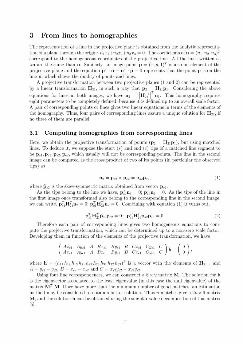
3 From lines to homographies

The representation of a line in the projective plane is obtained from the analytic representa-tion of a plane through the origin: n1x1+n2x2+n3x3 = 0. The coefficients of n = (n1, n2, n3)

T

correspond to the homogeneous coordinates of the projective line. All the lines written asλn are the same than n. Similarly, an image point p = (x, y, 1)T is also an element of theprojective plane and the equation pT · n = nT · p = 0 represents that the point p is on theline n, which shows the duality of points and lines.

A projective transformation between two projective planes (1 and 2) can be representedby a linear transformation H21, in such a way that p2 = H21p1. Considering the above

equations for lines in both images, we have n2 =[H−1

21

]Tn1. This homography requires

eight parameters to be completely defined, because it is defined up to an overall scale factor.A pair of corresponding points or lines gives two linear equations in terms of the elements ofthe homography. Thus, four pairs of corresponding lines assure a unique solution for H21, ifno three of them are parallel.

3.1 Computing homographies from corresponding lines

Here, we obtain the projective transformation of points (p2 = H21p1), but using matchedlines. To deduce it, we suppose the start (s) and end (e) tips of a matched line segment tobe ps1,pe1,ps2,pe2, which usually will not be corresponding points. The line in the secondimage can be computed as the cross product of two of its points (in particular the observedtips) as

n2 = ps2 × pe2 = ps2pe2, (1)

where ps2 is the skew-symmetric matrix obtained from vector ps2.As the tips belong to the line we have, pT

s2n2 = 0; pTe2n2 = 0. As the tips of the line in

the first image once transformed also belong to the corresponding line in the second image,we can write, pT

s1HT21n2 = 0; pT

e1HT21n2 = 0. Combining with equation (1) it turns out,

pTs1H

T21ps2pe2 = 0 ; pT

e1HT21ps2pe2 = 0. (2)

Therefore each pair of corresponding lines gives two homogeneous equations to com-pute the projective transformation, which can be determined up to a non-zero scale factor.Developing them in function of the elements of the projective transformation, we have

(Axs1 Ays1 A Bxs1 Bys1 B Cxs1 Cys1 CAxe1 Aye1 A Bxe1 Bye1 B Cxe1 Cye1 C

)h =

(00

),

where h = (h11 h12 h13 h21 h22 h23 h31 h32 h33)T is a vector with the elements of H21 , and

A = ys2 − ye2, B = xe2 − xs2 and C = xs2ye2 − xe2ys2.Using four line correspondences, we can construct a 8× 9 matrix M. The solution for h

is the eigenvector associated to the least eigenvalue (in this case the null eigenvalue) of thematrix MT M. If we have more than the minimum number of good matches, an estimationmethod may be considered to obtain a better solution. Thus n matches give a 2n×9 matrixM, and the solution h can be obtained using the singular value decomposition of this matrix[5].

7

It is known that a previous normalization of data avoids problems of numerical compu-tation. As our formulation only uses image coordinates of observed tips, data normalizationproposed for points [9] has been used. In our case the normalization makes the x and ycoordinates to be centered in an image which has unitary width and height.

Equations (2) can be used as a residue to designate inliers and outliers with respect toa candidate homography. In this case the residue is an algebraic distance and the relevanceof each line depends on its observed length, because the cross product of the segment tips isrelated to its length.

Alternatively a geometric distance in the image can be used. It is obtained from the sumof the squared distances between the segment tips and the corresponding transformed line

d 2 =(pT

s1HT21ps2pe2)

2

(HT21ps2pe2)2

x + (HT21ps2pe2)2

y

+(pT

e1HT21ps2pe2)

2

(HT21ps2pe2)2

x + (HT21ps2pe2)2

y

, (3)

where subindexes ()x and ()y indicate first and second component of the vector respectively.Doing the same for both images and with both observed segments, the squared distance

with geometric meaning is:

d 2 =(pT

s1HT21ps2pe2)

2 + (pTe1H

T21ps2pe2)

2

(HT21ps2pe2)2

x + (HT21ps2pe2)2

y

+(pT

s2H−T21 ps1pe1)

2 + (pTe2H

−T21 ps1pe1)

2

(H−T21 ps1pe1)2

x + (H−T21 ps1pe1)2

y

(4)

3.2 Robust estimation

The least squares method assumes that all the measures can be interpreted with the samemodel, which makes it very sensitive to outliers. Robust estimation tries to avoid the outliersin the computation of the estimate.

From the existing robust estimation methods [6], we have initially chosen the least medianof squares method. This method makes a search in the space of solutions obtained fromsubsets of minimum number of matches. If we need a minimum of 4 matches to computethe projective transformation, and there are a total of n matches, then the search space willbe obtained from the combinations of n elements taken 4 by 4. As that is computationallytoo expensive, several subsets of 4 matches are randomly chosen. The algorithm to obtainan estimate with this method can be summarized as follows:

1. A Monte-Carlo technique is used to randomly select m subsets of 4 features.

2. For each subset S, we compute a solution in closed form HS.

3. For each solution HS, the median MS of the squares of the residue with respect to allthe matches is computed.

4. We store the solution HS which gives the minimum median MS.

A selection of m subsets is good if at least one of them has no outliers. Assuminga ratio ε of outliers, the probability of one subset to be good can be obtained [16] as,P = 1− [1− (1− ε)4]

m. Thus assuming a probability (1−P ) of mismatch the computation,

the number of subset m to consider can be obtained. For example, if we want a probabilityP = 0.99 of one of them being good, having ε = 35% of outliers, the number of subsets m

8

should be 24. Having ε = 70% of outliers the number of subsets m should be 566 and aminor quantile instead of the median must be selected. Anyway, a reduction of ten times inthe probability of mismatch the computation (P = 0.999) only yields a computational costof 0.5 times larger (m = 36 with ε = 35% and m = 849 with ε = 70%).

3.3 Rejecting wrong basic matches

Once the solution has been obtained, the outliers can be selected from those of higher residue.Good matches can be selected between those of residue smaller than a threshold. As in [6] thethreshold is fitted proportional to the standard deviation of the error that can be estimated[16] as,

σ = 1.4826 [1 + 5/(n− 4)]√

MS.

Assuming that the measurement error for in inliers is Gaussian with zero mean andstandard deviation σ, then the square of the residues is a sum of Gaussian variables andfollows a χ2

2 distribution with 2 degrees of freedom. Taking, for example, a 5% of probabilityof rejecting a line being correct, the threshold will be fixed to 5.99 σ2.

4 Final matches

From here on, we introduce the geometrical constraint imposed by the estimated homographyto get a bigger set of matches. Our objective here is to obtain at the end of the processmore good matches, also eliminating wrong matches given by the basic matching. Thusfinal matches are composed by two sets. The first one is obtained from the matches selectedafter the robust computation of the homography passing additionally an overlapping testcompatible with the transformation of the segment tips. The second set of matches isobtained taking all the segments not matched initially and those being rejected previously.With this set of lines, a matching process similar to the basic matching is carried out.However, now the matching is made to the nearest neighbor segment transformed with thehomography. The transformation is applied to the end tips of the image segments using thehomography H21 to find, not only compatible lines but also compatible segments in the sameline.

In the first stage of the matching process there was no knowledge of the camera motion.However in this second step the computed homography provides information about expecteddisparity and therefore the uncertainty of geometric variations can be reduced. So, a newtuning of σxm , σym , σθ and σl, is considered. To automate the process, a global reduction ofthese parameters has been proposed and tested in several situations, obtaining good resultswith reductions of about 1/5.

As the measurement noise (σ‖ and σ⊥) has not changed, the initial tuning of theseparameters is maintained in this second step. Note that the brightness compatibility set isthe initially computed, and therefore it is not repeated.

5 Different planes

When lines are in different planes, the corresponding homographies can iteratively be com-puted. Previously, we have explained how to determine a homography assuming that some

9

of the lines are outliers. The first homography can be computed in this way assuming thata certain percentage of matched lines are good matches and belong to a plane, and theother matches are bad or they cannot be explained by this homography. We do not havea priori knowledge about which plane of the scene is going to be extracted the first, butthe probability of a plane being chosen increases with the number of lines in it. The mostreasonable way to extract a second plane is eliminating the lines used to determine the firsthomography. Here we are assuming that lines belonging to the first plane do not belong tothe second, which is true except for the intersection line between both planes. This idea ofeliminating lines already used will apply if more planes are extracted.

On the other hand, in the multi-plane case the percentage of outliers for each homographywill be high even all the matches are good. As the least median of squares method has abreakdown point in 50% of outliers, we have used in this case the Ransac method [17] whichneeds a tuning threshold, but works with a less demanding breakdown point.

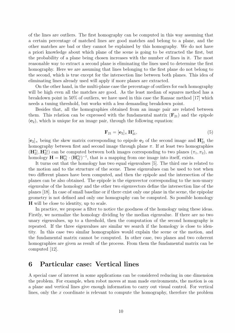
Besides that, all the homographies obtained from an image pair are related betweenthem. This relation can be expressed with the fundamental matrix (F21) and the epipole(e2), which is unique for an image pair, through the following equation:

F21 = [e2]×Hπ21, (5)

[e2]× being the skew matrix corresponding to epipole e2 of the second image and Hπ21 the

homography between first and second image through plane π. If at least two homographies(Hπ1

21 ,Hπ221) can be computed between both images corresponding to two planes (π1, π2), an

homology H = Hπ121 · (Hπ2

21)−1, that is a mapping from one image into itself, exists.

It turns out that the homology has two equal eigenvalues [5]. The third one is related tothe motion and to the structure of the scene. These eigenvalues can be used to test whentwo different planes have been computed, and then the epipole and the intersection of theplanes can be also obtained. The epipole is the eigenvector corresponding to the non-unaryeigenvalue of the homology and the other two eigenvectors define the intersection line of theplanes [18]. In case of small baseline or if there exist only one plane in the scene, the epipolargeometry is not defined and only one homography can be computed. So possible homologyH will be close to identity, up to scale.

In practice, we propose a filter to notice the goodness of the homology using these ideas.Firstly, we normalize the homology dividing by the median eigenvalue. If there are no twounary eigenvalues, up to a threshold, then the computation of the second homography isrepeated. If the three eigenvalues are similar we search if the homology is close to iden-tity. In this case two similar homographies would explain the scene or the motion, andthe fundamental matrix cannot be computed. In other case, two planes and two coherenthomographies are given as result of the process. From them the fundamental matrix can becomputed [12].

6 Particular case: Vertical lines

A special case of interest in some applications can be considered reducing in one dimensionthe problem. For example, when robot moves at man made environments, the motion is ona plane and vertical lines give enough information to carry out visual control. For verticallines, only the x coordinate is relevant to compute the homography, therefore the problem

10

is simplified. The homography now has three parameters and each vertical line gives oneequation, therefore three vertical line correspondences are enough.

The matching is quite similar to the presented for the lines in all directions. In thiscase the parameter referred to the orientation of the lines is discarded because it has nosense, although the lines are grouped in two incompatible subsets, those having 90 degreesof orientation and those with 270 degrees of orientation.

6.1 Estimation of the homography

In this case, as the dimension of the problem is reduced, only the xm coordinate is relevantfor the computation of the projective transformation H21. We can use the point basedformulation which is simpler because a vertical line can be projectively represented as apoint with (xm, 1) coordinates. Then, we can write, up to a scale factor

(λ xm2

λ

)=

(h11 h12

h21 h22

) (xm1

1

)

Therefore each pair of corresponding vertical lines having xm1 and xm2 coordinates re-spectively provides one equation to solve the matrix H21

(xm1 1 −xm1xm2 −xm2

)

h11

h12

h21

h22

= 0.

With the coordinates of at least n = 3 vertical line correspondences we can constructa n × 4 matrix M. The homography solution is the eigenvector associated to the leasteigenvalue of the MTM matrix.

As above before, we use a robust method to compute the projective transformation. Withvertical lines the problem is computationally simpler. For example with P = 0.99 and 70%of outliers only 168 sets of 3 matches must be considered (in the general case we need 566sets of 4 matches). As told before, the estimated homography is also used to obtain a betterset of matched lines.

7 Experimental Results

A set of experiments with different kind of images has been carried out to test the proposal.The images correspond to different applications: Indoor robot homing, images of buildings,and aerial images.

In the algorithms there are extraction parameters to obtain more or less line segmentsaccording to its minimum length and minimum gradient. There are also parameters to matchthe lines, whose tuning has turned out simple and quite intuitive. In the experiments we haveused the following tuning parameters σ⊥ = 1, σ‖ = 10, σagl = 8, σc = 4, σxm = 60, σym =20, σθ = 2, σl = 10, or small variation with respect to them depending on expected imagedisparity.

We have applied the algorithm presented for robot homing. In this application the robotmust go to previously learnt positions using a camera [10]. The robot corrects its headingfrom the computed projective transformation between target and current images. In this

11

Robot Rotation σxm Basic After H21 Final

2◦ 60 92 (1W) 78 (0W) 90 (0W)4◦ 60 73 (5W) 56 (1W) 76 (0W)6◦ 60 63 (4W) 47 (1W) 63 (0W)8◦ 60 53 (6W) 31 (0W) 52 (0W)10◦ 60 47 (9W) 35 (1W) 50 (0W)12◦ 100 41 (9W) 30 (2W) 33 (1W)14◦ 100 36 (12W) 24 (2W) 32 (1W)16◦ 100 27 (9W) 17 (3W) 30 (1W)18◦ 140 37 (14W) 24 (3W) 28 (1W)20◦ 140 28 (10W) 17 (1W) 24 (0W)

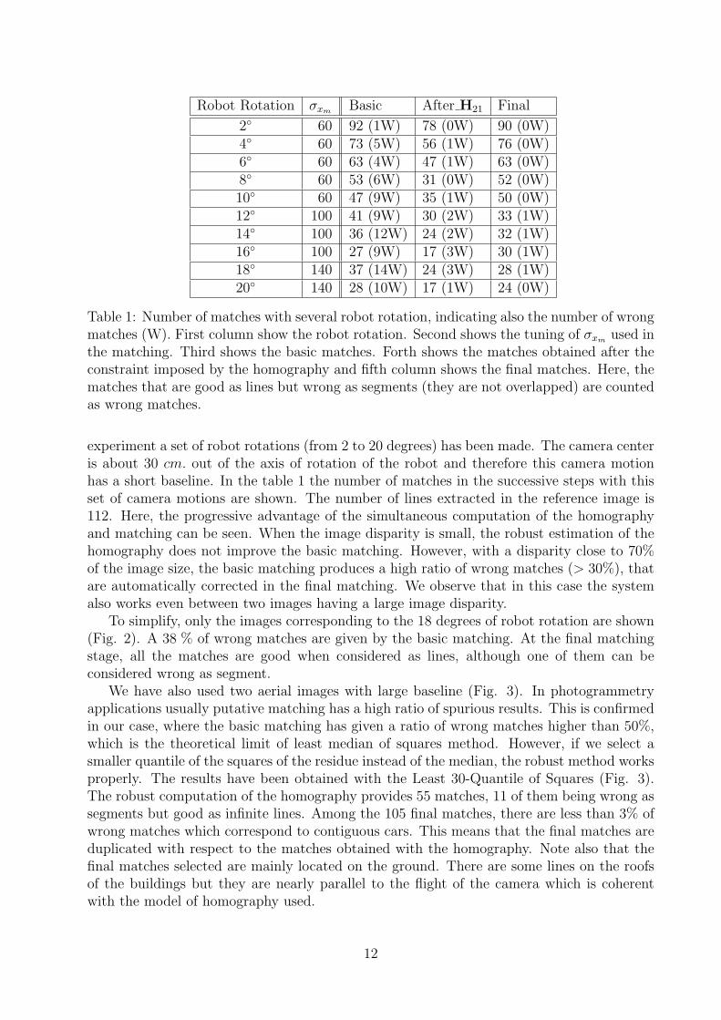
Table 1: Number of matches with several robot rotation, indicating also the number of wrongmatches (W). First column show the robot rotation. Second shows the tuning of σxm used inthe matching. Third shows the basic matches. Forth shows the matches obtained after theconstraint imposed by the homography and fifth column shows the final matches. Here, thematches that are good as lines but wrong as segments (they are not overlapped) are countedas wrong matches.

experiment a set of robot rotations (from 2 to 20 degrees) has been made. The camera centeris about 30 cm. out of the axis of rotation of the robot and therefore this camera motionhas a short baseline. In the table 1 the number of matches in the successive steps with thisset of camera motions are shown. The number of lines extracted in the reference image is112. Here, the progressive advantage of the simultaneous computation of the homographyand matching can be seen. When the image disparity is small, the robust estimation of thehomography does not improve the basic matching. However, with a disparity close to 70%of the image size, the basic matching produces a high ratio of wrong matches (> 30%), thatare automatically corrected in the final matching. We observe that in this case the systemalso works even between two images having a large image disparity.

To simplify, only the images corresponding to the 18 degrees of robot rotation are shown(Fig. 2). A 38 % of wrong matches are given by the basic matching. At the final matchingstage, all the matches are good when considered as lines, although one of them can beconsidered wrong as segment.

We have also used two aerial images with large baseline (Fig. 3). In photogrammetryapplications usually putative matching has a high ratio of spurious results. This is confirmedin our case, where the basic matching has given a ratio of wrong matches higher than 50%,which is the theoretical limit of least median of squares method. However, if we select asmaller quantile of the squares of the residue instead of the median, the robust method worksproperly. The results have been obtained with the Least 30-Quantile of Squares (Fig. 3).The robust computation of the homography provides 55 matches, 11 of them being wrong assegments but good as infinite lines. Among the 105 final matches, there are less than 3% ofwrong matches which correspond to contiguous cars. This means that the final matches areduplicated with respect to the matches obtained with the homography. Note also that thefinal matches selected are mainly located on the ground. There are some lines on the roofsof the buildings but they are nearly parallel to the flight of the camera which is coherentwith the model of homography used.

12

1

2

3 4 56

78

9

10

11

12

1314

1516

17

18 1920

21

22

23 2425 26

27

28

29

3031

3233 34

35

36

37

1

2

3 45

6

78

9

10

11

12

13

14

15

16

17

181920

21

22

232425

26

27

28

29

3031

32

33

34

35

3637

1

2

3

4

5

67

8

9

10 1112

13

14

15

16

17

18

19

20

21

22

2324 25

2627

28

1

2

3

4

5

67

8

9

101112

13

14

15

16

17

18

19

20

21

22

2324 25

2627

28

Figure 2: Images with 18 degrees of robot rotation. Images of first row show the matchesafter the basic matching (37 matches, 14 wrong). Second row shows the matches at thefinal stage of the process, only one been wrong match as segment although it is good as line(number 10).

13

�������������������������������������������������������������������������������������������������������������������������������������������������������������������������������������������������������������������������������������������������������������������������������������������������������������������������������������������������������������������������������������������������������������������������������������������������������������������������������������������������������������������� ��������������������������������������������������������������������������������������������������������������������������������������������������������������������������������������������������������������������������������������������������������������������������������������������������������������������������������������������������������������������������������������������������������������������������������������������������������������������������������������������������������������������

1 23

4

5 6

78

910

11

12 13

14

15

16

1718

192021

22 23

24

252627

28

2930

31

32333435

363738

39 4041

42

434445

4647 4849

50 51

525354

5556

57

5859

6061

62

63

64

65

66

6768 69

70

71

7273

747576

7778

7980

81

82

838485

86

87 8889 9091

929394

959697

9899100

101 102103104

105 106107

108109

110

111

112

113

114115

116

117118

119120

121

1234

5

6

7

8

9

101112

1314

15

16

1718

19 20

21

22

23

24

25

26

27

28

293031

32

33

34

35

3637

38

39

4041

42

43

4445

4647 48

49

5051

5253 545556

57

58 59

60

61

62

63

64

65

66

67

68

69

70

71

7273

74

75 76

77

78

79

8081 8283

8485

86

87

888990

91

92

93 94 9596

97

98

99

100

101

102103

104

105 106107108 109

110

111

112

113

114115

116

117118

119120

121

1

23

4

5

6

7

8

910

11

12

13

14

15

1617

1819

20

21

22

2324

25

26

27

28

2930

31

3233

34

3536

37

3839

4041

42

43 44

4546

47

4849

5051525354 55

56

57 585960

6162 6364

6566

6768 697071

7273747576 7778

79 80 8182

8384 85

8687 88 8990

9192

93

94

95 96 9798

99

100101

102

103104 105

1

23

4

5

6

7

8

9

10

11

12

13

14

15

16

17

18

19

20

21

22

2324

25

26

27

28

29303132

33

34

3536

37

383940

4142

4344

454647

4849

5051525354 55

56

57

585960

61

62

6364

6566

67

68

697071

7273

747576

77787980 81

828384

85

86

8788

89909192

9394

95

9697

98

99100101

102

103104 105

Figure 3: Two aerial images with large baseline. In the first row, the lines extracted aresuperimposed to the images (approximately 300 lines/image). The second row shows thebasic matches (121 matches, 64 being wrong). Third row shows the matches at the finalstage (105 matches, 3 being wrong that are corresponding to contiguous cars).

14

1

2

3

4

5

6 7

89

10

11

12

13

14151617 1819 2021

2223

24252627

28

29

30

313233 3435

36

37

38

394041

42 43

44

1

2

3

45

67

89

10

11

12

13

14151617 1819 2021

2223

242526 2728

29

30

313233 3435

36

37

38

3940

41

42 43

44

1

2

34

56

78

9

10

11

12

13

14

15

16

17

18

1920

2122

2324

25

26

27

28

29

30

1

2

34

5

6

78

9

10

11

12

13

14

15

16

17

18

1920

2122

2324

25

26

27

28

29

30

Figure 4: Two examples of image pairs with automatically matched vertical lines.

Basic.Matches Good Final.Matches GoodHouse 148 75% 114.6 (8.91) 99% (1%)College 196 82% 156.7 (11.09) 96% (1%)

Table 2: Number of matches of scenes in Figs. 5 and 6. Only the lines on the two mainplanes are considered. We have repeated the experiments fifty times using the same basicmatches, showing as final matches the mean values and, in brackets, the standard deviation.

We also show two examples of matched vertical lines with an homography of reduceddimension (Fig. 4). In both cases the percentage of good final matches is close to 100%.Using vertical lines, we have developed a real time implementation for robotic applicationsin man made environments [10].

Other experiments have been carried out to match lines which are in several planes,segmenting simultaneously the planes (Figs. 5, 6). In Table 2 we show the number ofmatches and the ratio of good matches for 50 repetitions of the robot computation. In thiscase, once an homography has been computed, the robust homography computation andthe growing of matches process has been iteratively repeated twice. As it can be seen, thenumber and quality of the final matches is very good. The homology filter just commentedin section 5 has been used to detect situations where a second plane is not obtained andtherefore a sole homography can be computed, or when the homographies do not give aright homology due to noise or bad extraction. It can be seen that some lines of the secondplane have been selected by the first homography (Fig. 6). The reason is that these linesare nearly coincident with epipolar lines and they can be selected by any homography beingcompatible with the fundamental matrix.

The method also work with rotated images. In this case σθ must be changed accordingto the image disparity. We show an example of a rotated image pair of short baseline wherea sole homography gives very good results (Fig. 7).

15

1 2

3

45

6 7

8

9

101112

13

14

151617

18

19

20

21

2223

24 2526

2728 29

30

3132

33

34

3536

3738

394041

42

43

44

45

464748 49

50 51

52

53 5455

565758

59

60

61

62

63

6465

66

67

68 69

70

7172

73

74 757677 7879 80

81

82838485

8687

88 8990 91 9293 94

9596

97

98 99100

101 102103 104

105106

107

108

109

110111

112

113114

115116 117118 119

120121 122

123

124

125

126

127

128

129

130

131

132

133

134135

136 137

138

139140

141142

143

144

145

146

147

1

2

3

45

67

8

9

101112

13

14

1516

1718

19

20

21

22 23

24 25

262728

29

30

3132

33343536

3738

39

40

41

42

43

44

45

46

474849

50 51

52

53 54

55

565758

5960 61

62

63

6465

66

67

68 69

70

7172

73

74

75

767778

7980

81

8283

8485

8687

88 8990 91 92

93

94

9596

97

98 99100101

102

103 104

105106107

108109

110111 112

113114

115116 117

118 119

120121 122

123124

125

126

127

128

129

130

131

132

133134

135136

137

138 139140

141142

143

144

145

146

147

1

2

34

5

678

9101112

131415 16

17

1819

2021

22

23

2425

262728

29

30 31 32

3334 3536

37 38

39 4041

4243444546

47484950

5152

53

54

55

56

57

58

59

60

61

62

63

64

65

6667

68

69

707172 73

7475

7677

78

79

80

1

23

4

5

678

9101112

131415 16

17

1819

2021

22

23

2425

262728

29

3031 32

3334

35

36

3738

3940

41 4243444546

47484950

5152

53

54

55

56

57

5859

60

61

62

63

64

65

66

67

68

69

70

717273

7475 7677

78

79

80

1

23 45

6 78

9

10

11

12

13

14151617

18

19

20

2122

232425

26

27

28

29

303132

33

34

35

3637

383940

41

424344

45

46 4748 49

50

51

52

1

2 3 4

5

6 78

9

10

11

12

13

14 151617

18

19

20

2122

2324

2526

27

28

29

303132

33

34

35

3637

383940

41

424344

45

46 4748 49

5051

52

Figure 5: Images of the house. First row: basic matches. Second row: final matchescorresponding to the first homography. Third row: final matches corresponding to secondhomography (Original images from KTH, Stockholm).

16

1

2 3

4

5678

910

1112

1314

15

1617

1819

2021

22

23

24

25

262728293031

32333435

3637

38 394041 42

434445

46

47 4849

50 5152 53 545556

5758

59 60

6162

63

6465

66

676869

7071

72

737475 76

7778

7980 81

82

83

84 8586 8788 8990 919293

1

23

4

567

8

9

10

11121314

15

1617

18 192021

22

23

24

25

262728293031

32333435

3637

38 394041 42

434445

46

474849

505152 53 545556

5758

59 60

61

62

6364

65

66

676869

70

71

72

7374 7576

7778

798081

82

83

848586

87888990 91

92

93

12

345

6

789 10

11

12

131415

161718

19

20

21222324

2526

27 28 29

30 313233 34

35 36 3738

39

4041

42

43

44

45

46

47

48

49

50 51

52535455

565758 5960

61

62

63

6465

66

6768

69

70

71

72

73

74

1 23 4

5 67

89

10

1112

131415

161718

19

20

21222324

2526

27 2829

30 313233 34

3536 3738

39

4041

42

43

44

45

46

47

48

49

50 51

52535455

565758 596061

62

63

64

65

66

6768

69

70

71

72

73

74

Figure 6: Images of the college. First row: basic matches. Second row: final matchescorresponding to first homography. Third row: final matches corresponding to second ho-mography (Original images from VGG, Oxford).

17

1

23

4

5 6

7

8

9

10

1112

1314

15

16

1718

19

202122

2324

25 2627

2829

30

3132

3334

35

36

37

3839

40

4142

43

44

45464748

4950 5152

53

54

555657 5859

60 61

62636465

6667

6869

70 7172

73

747576

77

78

7980

81

828384

858687 8889 9091

9293

94

9596

97 9899

100

101

102

103 104105

106

107

108

109

110 111

112

113114 115116117

1

23

4

5

6

7

8

9

10

11

12

13

14

15

16

17

18

19

20

2122

2324

25

26

27

2829

30

31

32

33

34

35

36

37

38

39

40

41

42

43

44

45

464748

49

50

51

5253

545556

57

58

59

60

61

6263

64

65

6667

6869

70

7172

73

74

7576

77

78

79

80

81

82

83

84

85

86

87

88

89

90

91

92

93

94

95

96

97

98

99

100

101

102

103

104105

106

107

108 109

110

111

112

113114

115

116

117

1

23

4

5 6

7

8

9

10

1112

1314

15

16

1718

19

202122

232425 26

27

2829

30

3132

3334

35

36

37

3839

40

4142

43

44

45464748 49

50 5152

53

54

555657 5859

60 61

62636465 6667

6869

70 7172

73

747576

77

78

7980

81

828384

858687 8889 9091

9293

94

9596

97 9899

100

101

102

103 104105

106

107

108

109

110 111

112

113114 115116

117

1

23

4

5

6

7

8

9

10

11

12

13

14

15

16

17

18

19

20

2122

2324

25

26

27

2829

30

31

32

33

34

35

36

37

38

39

40

41

42

43

44

454647

48

49

50

51

5253

545556

57

58

59

60

61

6263

64

65

6667

6869

70

7172

73

74

7576

77

78

79

80

81

82

83

84

85

86

87

88

89

90

91

92

93

94

95

96

97

98

99

100

101

102

103

104105

106

107

108 109

110

111

112

113114

115

116117

Figure 7: Pair of rotated short baseline images and final line correspondences.

18

8 Conclusions

We have presented and tested a method to automatically obtain matches of lines simultane-ously to the robust computation of homographies in image pairs. The robust computationworks especially well to eliminate outliers which may appear when the matching is basedon image properties and there is no information of scene structure or camera motion. Thehomographies are computed from lines extracted and the use of lines has advantages withrespect to the use of points. The geometric mapping between uncalibrated images providedby the homography turns out useful to grow matches and to eliminate wrong matches.

All the work is automatic with only some previous tuning of parameters related to theexpected global image disparity. As is seen in the experiments, the proposed algorithm workswith different types of scenes. With planar scenes or in situations where disparity is mainlydue to rotation, the method gives good results with only one homography. However, it isalso possible to compute several homographies when several planes are in the scene, whichare iteratively segmented. In this case, the fundamental matrix can be computed from linesthrough the homographies, obtaining a constraint for the whole scene. Currently we areworking with other image invariants to improve the first stage of the process.

Acknowledgments

This work was supported by project DPI2003-07986.

References

[1] C. Schmid and A. Zisserman, “Automatic Line Maching across Views,” In IEEE Con-ference on CVPR, pp. 666–671 (1997).

[2] D. G. Lowe, “Distinctive image features from scale-invariant keypoints,” InternationalJournal of Computer Vision 60(2), 91–110 (2004).

[3] H. Bay, V. Ferrari, and L. V. Gool, “Wide-Baseline Stereo Matching with Line Seg-ments,” In IEEE Conference on Computer Vision and Pattern Recognition, volume 1,329–336 (2005).

[4] P. Pritchett and A. Zisserman, “Wide Baseline Stereo Matching,” In IEEE Conferenceon Computer Vision, pp. 754–760 (1998).

[5] R. Hartley and A. Zisserman, Multiple View Geometry in Computer Vision (CambridgeUniversity Press, Cambridge, 2000).

[6] Z. Zhang, “Parameter Estimation Techniques: A tutorial with Application to ConicFitting,” Rapport de recherche RR-2676, I.N.R.I.A., Sophia-Antipolis, France (1995) .

[7] P. Torr and D. Murray, “The Development and Comparison of Robust Methods forEstimating the Fundamental Matrix,” International Journal of Computer Vision 24,271–300 (1997).

19

[8] L. Quan and T. Kanade, “Affine Structure from Line Correspondences with Uncali-brated Affine Cameras,” IEEE Trans. on Pattern Analysis and Machine Intelligence19(8), 834–845 (1997).

[9] R. Hartley, “In Defense of the Eight-Point Algorithm,” IEEE Trans. on Pattern Analysisand Machine Intelligence 19(6), 580–593 (1997).

[10] J. Guerrero, R. Martinez-Cantin, and C. Sagues, “Visual map-less navigation based onhomographies,” Journal of Robotic Systems 22(10), 569–581 (2005).

[11] A. Habib and D. Kelley, “Automatic relative orientation of large scale imagery overurban areas using Modified Iterated Hough Transform,” Journal of Photogrammetryand Remote Sensing 56, 29–41 (2001).

[12] C. Sagues, A. Murillo, F. Escudero, and J. Guerrero, “From Lines to Epipoles ThroughPlanes in Two Views,” Pattern Recognition (2006), to Appear.

[13] J. Guerrero and C. Sagues, “Robust line matching and estimate of homographies si-multaneously,” In IbPRIA, Pattern Recognition and Image Analysis, LNCS 2652, pp.297–307 (2003).

[14] J. Burns, A. Hanson, and E. Riseman, “Extracting Straight Lines,” IEEE Trans. onPattern Analysis and Machine Intelligence 8(4), 425–455 (1986).

[15] R. Deriche and O. Faugeras, “Tracking Line Segments,” In First European Conferenceon Computer Vision, pp. 259–268 (Antibes, France, 1990).

[16] P. Rousseeuw and A. Leroy, Robust Regression and Outlier Detection (John Wiley, NewYork, 1987).

[17] M. A. Fischler and R. C. Bolles, “Random Sample Consensus: A Paradigm for ModelFitting with Applications to Image Analysis and Automated Cartography,” Comm. ofthe ACM 24(2), 381–395 (1981).

[18] L. Zelnik-Manor and M. Irani, “Multiview Constraints on Homographies,” IEEE Trans-actions on Pattern Analysis and Machine Intelligence 24(2), 214–223 (2002).

20