Robust Gas Turbine and Airframe System Design in

Light of Uncertain Fuel and CO2 Prices

Stephan Langmaak1, James Scanlan2, and András Sóbester3

University of Southampton, Southampton, SO16 7QF, United Kingdom

This paper presents a study that numerically investigated which cruise speed the

next generation of short-haul aircraft with 150 seats should �y at and whether a con-

ventional two- or three-shaft turbofan, a geared turbofan, a turboprop, or an open

rotor should be employed in order to make the aircraft's direct operating cost robust

to uncertain fuel and carbon (CO2) prices in the Year 2030, taking the aircraft pro-

ductivity, the passenger value of time, and the modal shift into account. To answer

this question, an optimization loop was set up in MATLAB consisting of nine modules

covering gas turbine and airframe design and performance, �ight and aircraft �eet sim-

ulation, operating cost, and optimization. If the passenger value of time is included,

the most robust aircraft design is powered by geared turbofan engines and cruises at

Mach 0.80. If the value of time is ignored, however, then a turboprop aircraft �ying

at Mach 0.70 is the optimum solution. This demonstrates that the most fuel-e�cient

option, the open rotor, is not automatically the most cost-e�cient solution because of

the relatively high engine and airframe costs.

1 Research Engineer, Computational Engineering and Design2 Professor of Aerospace Design, Computational Engineering and Design, AIAA member3 Associate Professor in Aircraft Engineering, Computational Engineering and Design, AIAA member

1

I. Introduction

A. Background

IT takes around 5 years to develop a gas turbine engine, which then usually remains in pro-

duction for more than two decades [1, 2]. Similar to the rest of the aerospace industry, gas turbine

makers therefore have to make multi-billion investments into these large and long-term projects and

it normally takes at least 15 years until the costs are recuperated [1]. Consequently, the strategic

design team must make a sound prediction 30 years into the future and optimize the product in

such a way that it remains competitive throughout that period.

The Advisory Council for Aeronautics Research in Europe (ACARE) [1] states: �The future is

uncertain, except that changes will be rapid and marked, especially in the price of resources, and

this scenario will become a normal phenomenon.� Such uncertainties led to the development of

the principle known as `robust design', which involves a departure from the classic search for the

global optimum. Instead, objective function plateaus are sought that balance nominal performance

against performance variability [3]. Thus, the System Study presented in this paper uses a `robust

design' methodology to �nd the optimum cruise speed, gas turbine and airframe to minimize the

direct operating cost of the next generation of short-range 150-seat aircraft in light of uncertain oil

and carbon (CO2) prices in the Year 2030.

Although 2030 is less than two decades away, this timeframe was chosen because 2025 to 2030

is the likely service entry window for the next generation of short-range aircraft [4]. In the 2020s,

the engine system options described in Section II will also be mature enough to potentially be used

on such an airframe. No prognosis beyond the Year 2030 is made because of the unpredictability

of many factors thereafter, not just oil and carbon prices, but also technological capabilities and

aircraft rollout dates [5].

1. Relevance of Work

The signi�cance of the System Study is re�ected in the richness of the literature on the subject,

some of which is captured in Table 1. Although as a whole the 11 references listed in Table 1

cover most of the work carried out in the System Study, each reference primarily focuses on one of

2

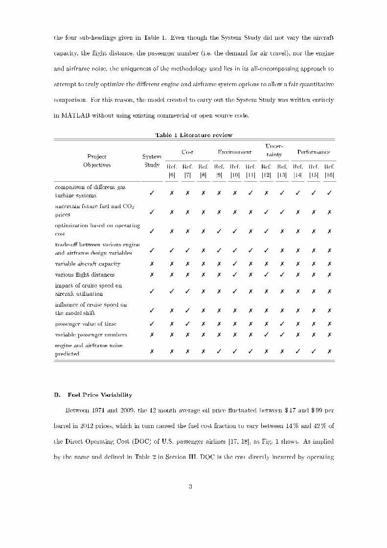
the four sub-headings given in Table 1. Even though the System Study did not vary the aircraft

capacity, the �ight distance, the passenger number (i.e. the demand for air travel), nor the engine

and airframe noise, the uniqueness of the methodology used lies in its all-encompassing approach to

attempt to truly optimize the di�erent engine and airframe system options to allow a fair quantitative

comparison. For this reason, the model created to carry out the System Study was written entirely

in MATLAB without using existing commercial or open source code.

Table 1 Literature review

Uncer-Cost Environment tainty Performance

Project System

Ref. Ref. Ref. Ref. Ref. Ref. Ref. Ref. Ref. Ref. Ref.Objectives Study

[6] [7] [8] [9] [10] [11] [12] [13] [14] [15] [16]

comparison of di�erent gasturbine systems 3 7 7 7 7 7 3 7 3 3 3 3

uncertain future fuel and CO2

prices 3 7 7 7 7 7 7 3 3 7 7 7

optimization based on operatingcost 3 7 7 7 3 3 7 3 7 7 7 7

trade-o� between various engineand airframe design variables 3 3 3 7 3 3 3 3 7 7 7 7

variable aircraft capacity 7 7 7 7 7 3 7 7 7 7 7 7

various �ight distances 7 7 7 7 7 3 7 3 3 7 7 7

impact of cruise speed onaircraft utilization 3 3 3 7 7 3 7 7 7 7 7 7

in�uence of cruise speed onthe modal shift 3 7 3 7 7 7 7 7 7 7 7 7

passenger value of time 3 7 3 7 7 7 7 7 3 7 7 7

variable passenger numbers 7 7 7 7 7 7 7 3 3 7 7 7

engine and airframe noisepredicted 7 7 7 7 3 3 3 7 7 3 3 7

B. Fuel Price Variability

Between 1971 and 2009, the 12-month average oil price �uctuated between $ 17 and $ 99 per

barrel in 2012 prices, which in turn caused the fuel cost fraction to vary between 14% and 42% of

the Direct Operating Cost (DOC) of U.S. passenger airlines [17, 18], as Fig. 1 shows. As implied

by the name and de�ned in Table 2 in Section III, DOC is the cost directly incurred by operating

3

an aircraft, i.e. (1) the cost of fuel; (2) engine and airframe depreciation and maintenance costs;

(3) landing, navigation, crew and ground charges. In July 2008, for example, jet fuel prices peaked

at $ 4.33 per U.S. gallon, but plummeted to $ 1.28 by late December that year [19]. Similarly,

between June 2014 and January 2015 the oil price dropped from around $ 110 to below $ 50 per

barrel [20]. This short-term volatility is caused by market inelasticity both on the supply and the

demand side, which means that small changes on either side of the economic equation have a large

e�ect on price [21].

Fig. 1 Correlation between oil price and direct operating cost from 1971 to 2009 (based on

data from Refs. [17, 18, 22]).

According to various forecasts, oil prices will continue to increase and exhibit increasing volatil-

ity [1, 21]. The uncertainty of future oil prices is re�ected by the U.S. Energy Information Admin-

istration's (EIA) large price disparity between the best and worst case scenarios for 2030 of around

73 and 196 $/barrel in 2012 prices, respectively [18, 23]. The United Kingdom (UK) Department

of Energy & Climate Change concurs with that prediction [24]. As in the past, the impact of in-

creasing fuel prices can be minimized by e�ciency gains, which, as this paper will show, is partly

made possible by advanced gas turbine technology in combination with an airframe optimized for

4

the most cost-e�cient cruise speed.

C. Carbon Trading

In 2009, the UK's House of Commons Transport Committee [4] stated that the cost of jet fuel

does not provide enough incentive to achieve signi�cant emission reductions and encourage airlines

to operate the latest generation of aircraft. An additional charge is therefore required whereby

1 metric-ton of CO2 emissions would have to cost between e 100 and e 300 [4], i.e. around $ 131

to $ 392 in 2012 prices [18, 25]. Based on U.S. passenger airlines data [17], in 2009 an aircraft had

to �y approximately 5,400mi on an 11-hour �ight from Seattle to Beijing, for example, in order to

emit 1 metric-ton of CO2 per passenger.

As economic instruments are more cost-e�cient and �exible in comparison to �xed regula-

tion [26], the British government, the aviation industry, as well as environmental groups believe

that for the international airline industry, international emission trading across all industrial sec-

tors is the best solution [27, 28]. Since 2012, all �ights within the European Union (EU) with a

maximum take-o� weight above 5,700 kg are therefore obliged to participate in the EU's Emission

Trading Scheme [26, 29].

Considering that CO2 was traded at approximately e 6 (≈ $ 8) per metric-ton in 2014 [25, 30]

shows that currently the EU Emission Trading Scheme has a relatively small impact on ticket prices

in comparison to the fuel cost. However, the UK's Committee on Climate Change published low-

and high-price scenarios for 2030 of ¿ 35 and ¿ 105 (around $ 62 to $ 186) per metric-ton of CO2 in

2012 prices [5, 18, 25].

II. Gas Turbine and Airframe System Options

For the next-generation 150-seater, the gas turbine and airframe manufacturers are exploring

�ve aircraft system options: the two- and three-shaft turbofan, the geared turbofan, the turboprop,

and the open rotor [31�33]. Thus, this study modelled these �ve system options in conjunction with a

fuselage, gear, �aps, slats, and spoilers based on the current Airbus A320 [34], as shown in Figs. 2�7,

because it is unlikely that a radically new design, like the �ying wing, will be introduced by 2030 [5,

27]. While the three turbofan options all use the conventional low-wing airframe layout where

5

the engines are mounted under the wing as illustrated in Figs. 2�4, the turboprop-powered aircraft

displayed in Fig. 5 requires four engines installed on a high wing to provide enough ground clearance

for the propeller tips. Both the wing and gear fairing in Fig. 5 are based on the BAe Avro RJ [34].

As the open rotor has two propellers mounted in tandem, Figs. 6 and 7 show that only two engines

are installed at the rear of a low-wing fuselage. The di�erence between the aircraft in Fig. 6 and

Fig. 7 is that the former is designed for a cruise speed of Mach 0.70, while the latter is optimized

for Mach 0.76 which therefore has greater wing and tail sweep angles.

Each of the �ve system options is explained in more detail in the following sub-sections. In

order to keep a clear distinction between the engine and the rest of the aircraft, the word `airframe'

is used where the term `aircraft' might be more appropriate. Similarly, the open rotor blades are

referred to as `propellers' to avoid confusion with the rest of the engine.

A. System Option 1: Two-Shaft Turbofan

First tested on the Rolls-Royce Olympus engine in 1950 [35], the inner shaft of the two-shaft

turbofan connects the slower turning fan, the low-pressure compressor (LPC), and low-pressure

turbine (LPT), while the outer shaft links the high-speed high-pressure compressor (HPC) and

high-pressure turbine (HPT). The two-shaft turbofan shown schematically in Fig. 2a consists of one

fan, three LPC, nine HPC, two HPT, and six LPT stages. For simplicity, the shafts are not shown

in Fig. 2a nor in any other engine schematic in this paper.

6

a) Engine b) Airframe plan view

c) Airframe front view d) Airframe side view

Fig. 2 Two-shaft turbofan aircraft (cruise speed: Mach 0.78).

B. System Option 2: Three-Shaft Turbofan

First certi�ed on the RB211 engine in 1972 [36], an additional intermediate-pressure system

increases e�ciency and reduces engine length and weight, but leads to higher complexity and cost [2].

The three-shaft engine in Fig. 3 has one fan, seven intermediate-pressure compressor (IPC), six HPC,

one HPT, one intermediate-pressure turbine (IPT), and six LPT stages.

7

a) Engine b) Airframe plan view

c) Airframe front view d) Airframe side view

Fig. 3 Three-shaft turbofan aircraft (cruise speed: Mach 0.78).

C. System Option 3: Geared Turbofan

Instead of using a third shaft, the rotational speed of the fan can also be uncoupled from the

low-pressure system by installing a planetary gear system between the fan and the LPC, as was �rst

�ight demonstrated on the Pratt & Whitney PW1000G in 2008 [37]. The e�ect of the planetary

gear system, represented by the rectangular box between the fan and the LPC in Fig. 4a, on the

engine design can clearly be seen by comparing Fig. 4a to Fig. 2a which have similar performance

characteristics. Due to the increased rotational speed of the LP system, Fig. 4a only has three LPT

stages while Fig. 2a has six.

8

a) Engine b) Airframe plan view

c) Airframe front view d) Airframe side view

Fig. 4 Geared turbofan aircraft (cruise speed: Mach 0.78).

D. System Option 4: Turboprop

As the weight and the drag of the nacelle limit the bypass ratio of the turbofan, the only way

to further increase e�ciency is by removing the fan duct and using a propeller instead of a fan, as

was �rst �ight tested on the experimental Meteor 1 with two Rolls-Royce Trent engines in 1945 [38].

The disadvantage of removing the protective fan duct is, however, that the axial speed of the air

entering the propeller is primarily determined by the �ight speed, rather than by the design of the

fan duct, which limits the turboprop's maximum cruise speed [2]. Similar to the geared turbofan,

the propeller is driven by the LPT through a reduction gearbox in order to limit the rotational

speed of the propeller and minimize the number of LPT stages. Despite the gearbox, the maximum

cruise speed is also restricted to prevent the air�ow velocity relative to the blade tips of the propeller

9

from exceeding the speed of sound, which would lead to a signi�cant rise in noise and drag [39]. At

present, the turboprop is consequently only used for shorter �ights where the reduced cruise speed

does not have a signi�cant e�ect on the trip time [40].

The turboprop shown in Fig. 5 is based on the Europrop International TP400-D6 engine [41]

which powers the Airbus A400M. Despite the higher mechanical complexity, the TP400-D6 is a

three-shaft con�guration because it allows the propeller to be independently powered by the LPT,

while the engine core has the operational �exibility of a two-shaft engine [39, 42]. The eight-bladed

propeller has a variable-pitch mechanism which means that a constant rotational speed can be

maintained independently of the thrust setting by adjusting the blade pitch angle [42, 43]. The

rotational speed is reduced as the cruise velocity is approached, however, to prevent the maximum

�ow velocity relative to the blade tips from exceeding Mach 0.95 [42]. Apart from the propeller, the

engine in Fig. 5a consists of four IPC, six HPC, one HPT, one IPT, and three LPT stages.

10

a) Engine b) Airframe plan view

c) Airframe front view d) Airframe side view

Fig. 5 Turboprop aircraft (cruise speed: Mach 0.70).

E. System Option 5: Open Rotor

Unlike the turboprop, the open rotor has two counter-rotating `propellers' that are arranged in

tandem. The second propeller not only increases the thrust produced, but it also recovers the air

swirl leaving the �rst propeller, which increases engine e�ciency and allows the open rotor to operate

at a higher cruise speed than the turboprop [31, 39], as Fig. 7 shows. Figure 1 in Section I indicates

that the open rotor concept designs were developed and tested in the 1980s as a consequence of the

OPEC oil embargo of 1973 but were cancelled by the end of the decade because of the reducing oil

prices [44]. Since the oil price peak in 2008, however, there has been a renewed interest in the open

rotor [45].

Of the �ve system options, the open rotor presents the most technological and operational chal-

11

lenges, however, including open rotor blade integration, control and reliability, engine installation

and noise [32, 46, 47]. The two propeller rows can either be installed at the front or the rear of

the engine, respectively known as the tractor and the pusher con�guration [31]. A further option

is whether the propellers are driven directly by a counter-rotating turbine or through a reduction

gearbox which requires cooling and increases mechanical complexity [47].

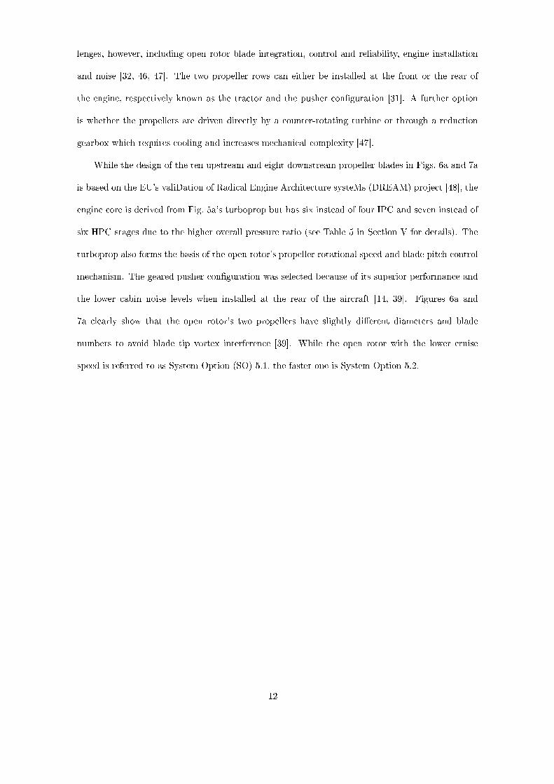
While the design of the ten upstream and eight downstream propeller blades in Figs. 6a and 7a

is based on the EU's valiDation of Radical Engine Architecture systeMs (DREAM) project [48], the

engine core is derived from Fig. 5a's turboprop but has six instead of four IPC and seven instead of

six HPC stages due to the higher overall pressure ratio (see Table 5 in Section V for details). The

turboprop also forms the basis of the open rotor's propeller rotational speed and blade pitch control

mechanism. The geared pusher con�guration was selected because of its superior performance and

the lower cabin noise levels when installed at the rear of the aircraft [14, 39]. Figures 6a and

7a clearly show that the open rotor's two propellers have slightly di�erent diameters and blade

numbers to avoid blade tip vortex interference [39]. While the open rotor with the lower cruise

speed is referred to as System Option (SO) 5.1, the faster one is System Option 5.2.

12

a) Engine b) Airframe plan view

c) Airframe front view d) Airframe side view

Fig. 6 Open rotor aircraft (cruise speed: Mach 0.70).

13

a) Engine b) Airframe plan view

c) Airframe front view d) Airframe side view

Fig. 7 Open rotor aircraft (cruise speed: Mach 0.76).

III. Multi-Objective Optimization

In theory, engineering design simply involves �nding and analyzing all conceivable designs and

then selecting the best one [49]. In order to �nd the best solution objectively, however, all signi�cant

design consequences have to be compared on an equal basis [50, 51]. Most real design problems

have more than one objective that has to be addressed, for example minimizing cost while meeting

a particular quality standard. These goals and constraints often con�ict, which means that the

objective functions have to be traded o� in some way [51].

There are several multi-objective optimization methods available, including Objective Aggre-

gation where all objectives are weighted and combined into one formula. Although monetary value

is a form of Objective Aggregation, there are many ways of measuring and optimizing it, as the

14

following sub-sections show.

A. Pro�t

Airlines try to increase their pro�t by maximizing their revenue and reducing their operating

costs. They consequently purchase aircraft (i.e. airframes and propulsion systems) that promise

a greater pro�t than investing the money in other assets, i.e. competing aircraft designs or even

di�erent business ventures or �nancial products [52]. The pro�tability of the aircraft in comparison

to other investments can be calculated using the Net Present Value (NPV) formula presented in

Eq. 1, which is derived from Refs. [50] and [52]. It is the sum of the present values of the yearly

operating pro�ts (i.e. the yearly revenues minus the total operating costs) generated during the

service life of the aircraft [52]. The depreciation of the aircraft is not included in the operating

costs, because it is accounted for in the aircraft acquisition cost which is subtracted separately.

While the airline revenue is primarily the sum of the passenger and freight tickets sold, the discount

rate is the annual interest other investments would generate [52]. Operating cost is covered in more

detail in the next sub-section.

NPVP =L∑

t=1

[Rt − TOCt

(1 + idis)t

]−AAC where

NPVP = net present value of pro�ts

L = aircraft service life in years

t = tth year of service

Rt = revenue for year t

TOCt = total operating cost for year t

(excl. aircraft depreciation)

idis = discount rate

AAC = aircraft acquisition cost

(1)

The gas turbine and airframe manufacturers are more likely to maximize their sales and hence

their pro�ts if they design an aircraft that maximizes the pro�t of the airlines. The best air-

craft design can therefore be found by maximizing Eq. 1. Net Present Value consequently enables

multi-objective optimization by expressing the aircraft's speci�cation in terms of monetary value.

Rather than applying subjective weightings to incompatible design requirements, like speci�c fuel

consumption and manufacturing cost where the optimum tradeo� is not immediately apparent, the

invisible hand of the market conducts the tradeo�. This means that when speci�c fuel consumption

is converted into fuel cost, the fuel price is used as the weighting parameter.

15

B. Operating Cost

The authors believe that the all-encompassing nature of Eq. 1 is its strength but also its weak-

ness, because a large dataset is required in order to model the entire service life of the aircraft. In

addition, it is particularly di�cult to estimate the airline revenue because ticket prices, passenger

numbers, and freight volume are controlled by many variables outside the engineering realm, in-

cluding economic, geographic, political, and time factors [53]. Although fuel and carbon prices in

2030 are similarly unpredictable as airline revenues, the fuel and carbon costs of an airline are also

in�uenced by the design of the aircraft through its fuel e�ciency. Assuming that aircraft safety,

noise and passenger appeal are not signi�cantly altered, the only aircraft performance metric that

has an impact on the revenue is the cruise speed. It a�ects the ticket prices and the number of

tickets sold through the value of time and the modal shift, respectively. The value of time and the

modal shift are respectively discussed in more detail in the next sub-section and in the Appendix.

Rather than modelling Eq. 1 in its entirety and obscuring the results by factors that are not

related to the design of the aircraft, the focus was laid on the total operating cost. According to

Doganis [54], total operating cost can be divided into direct and indirect operating costs, as shown

in Table 2.

Table 2 Direct and indirect operating cost (adapted from Ref. [54])

Direct Operating Cost Indirect Operating Cost

• aircraft depreciation (represented by AAC in Eq. 1) • ground buildings, equipment, and transport

• interest on aircraft • ground sta�

• aircraft insurance • ticketing, sales, and promotion

• aircraft maintenance • administration

• fuel and oil

• �ight crew

• cabin crew

• airport charges

• en-route charges

The Indirect Operating Cost (IOC) is primarily dependent on how the airline is run and is

16

therefore di�cult to estimate [52, 55]. For these reasons, IOC is usually ignored by the aircraft

designer [55] and consequently it was also not included in this study.

The DOC, on the other hand, is signi�cantly a�ected by the design of the aircraft [55]. As

a �gure of merit in economic analysis, aircraft comparison, and design tradeo� studies, DOC is

usually expressed in $ per seat-mile or $ per revenue-passenger-kilometer (RPK) �own [52]. This

accounts for the e�ect the load factor and the cruise speed have on the productivity of the aircraft.

As DOC is e�ectively the value of time (aircraft and crew) and resources consumed (fuel and oil),

it could also include the passengers' value of time [7]. Table 2 indicates that DOC includes aircraft

depreciation, which is equivalent to dividing Eq. 1's aircraft acquisition cost by the aircraft service

life, assuming that a simple linear depreciation method is used over the operating life of the aircraft.

Eq. 2 shows that the NPV of the Direct Operating Costs could be calculated in a similar way as for

the pro�ts in Eq. 1. The DOC for only one year of operation was calculated, however, because the

authors believe that the work involved in predicting uncertain cost data for every year of service

would not improve the accuracy of the result. The futility of fully modelling both Eq. 1 and Eq. 2 is

aggravated by the discount factor, which has the e�ect that costs incurred at the end of the service

life have a diminishing e�ect on the NPV. A further reason why Eq. 2 was not used in this study is

that the discount factor is another variable that is independent of the aircraft design.

NPVDOC =

L∑t=1

[DOCt

(1 + idis)t

](2)

Based on the arguments presented above, which are summarized in Table 3, the authors believe

that DOC covers all the aircraft-design related aspects of Eq. 1 and is therefore a good substitute

for the net present value of pro�ts.

17

Table 3 Comparison of NPVP and DOC parameters

Parameter NPVP DOC

aircraft service life t, L aircraft depreciation

ticket price R value of time (the only ticket price factor directly a�ected by the air-craft design, assuming that aircraft safety, noise, and passenger appealare not altered)

number of tickets sold R seat miles or RPK

Direct Operating Cost TOC included

Indirect Operating Cost TOC not included (not a�ected by the aircraft design)

discount factor idis not included (not a�ected by the aircraft design)

aircraft acquisition cost AAC aircraft depreciation

C. Cost of Time

Value of Time (VoT) is a concept often found in cost-bene�t analyses of transport services and

infrastructure [56]. In transport, it re�ects how much travelers are willing to pay to save time during

a journey and, conversely, how much monetary compensation they would expect for slow or delayed

transport [7, 56]. As with ticket prices, the value of time depends on many factors, including the

length, time, location, and itinerary of the journey, the mode of transport, the fare class, the purpose

of the trip, and other socio-economic characteristics of the passenger [56, 57]. As the value of time

is an opportunity cost, it only applies if the passenger has the opportunity to choose a faster mode

of transport, i.e. in this case a competing aircraft with a higher cruise speed [7, 56, 57].

For business passengers, the value of time is equivalent to their rate of pay minus the value of

the work done during the journey [56]. The value of non-working time can be found by analyzing

the transport choices leisure travelers make, based on journey time and cost [56]. Business pas-

sengers generally value time higher than leisure travelers [58], which is re�ected by ITA's [57] and

EUROCONTROL's [59] estimates for air travel: while business passengers' average value of time is

around e 67 (≈ $ 82) per hour in 2012 prices, it is only e 26 (≈ $ 32) per hour for tourists. Taking

the passenger distribution [57, 59] into account, this gives an average value of time of e 48 (≈ $ 58)

per hour.

18

D. Robust Design

There are several metrics for measuring robustness in which the tradeo� between the mean

and the variability of the objective function is weighted di�erently. While `minimax' optimization

involves minimizing the maximum value and is therefore a conservative approach because it optimizes

the worst-case scenario, Bayes Principle focuses on the average-case scenario by simply minimizing

the mean [3]. In this study, the Mean-Square Deviation (MSD), de�ned in Eq. 3, was minimized

because it takes both the mean and the variability into account and is therefore a compromise

between the other two approaches. Eq. 3 is adapted from Keane and Nair [3] where M represents

the sample number and yj is the jth sample of the objective function.

MSD =1

M

M∑j=1

y2j (3)

Although the reader might expect the slower but more fuel-e�cient turboprop to produce the most

robust design, the optimum solution is not that straightforward because of the following design

tradeo�s:

• As the cruise speed a�ects aircraft utilization, the optimization loop has to trade productivity

against fuel and carbon costs [7].

• Expensive gas turbine and airframe technology tends to reduce fuel consumption. Fuel and

carbon costs therefore have to be balanced against acquisition cost [7].

• A small wing area reduces parasitic drag which tends to improve cruise performance but it

leads to higher takeo� and landing speeds which requires more powerful engines [7].

The Airbus A380 has a much larger fan that increases fuel burn by 1�2% in order to meet night-time

noise restrictions at London Heathrow airport [27]. This shows that there is also a complex tradeo�

between emissions and noise [31]. Noise is not included in the optimization loop, however, because

of the complexity of predicting it as well as estimating its impact on the operating costs in 2030.

Considering that even the open rotor is likely to meet the International Civil Aviation Organization

(ICAO) Chapter 14 standard, that will take e�ect in 2020, shows that noise is unlikely to be a

critical design factor [60].

19

IV. System Design Methodology and Assumptions

Figure 8 shows the optimization framework set up in MATLAB to �nd the most robust engine

and airframe speci�cations for the �ve gas turbine options. As the exact thrust requirement for

each new aircraft con�guration is not known in advance, Fig. 8 indicates that Modules 1 and 2

�rst create provisional engine and airframe designs based on a takeo� thrust estimate of 124 kN

per turbofan engine, and a turboprop and open rotor LPT power output of 5.9MW and 18.0MW,

respectively. These thrust and power estimates are multiplied by a growth factor of 1.25 based on

the thrust ratio between the growth and the baseline version of the V2500 engine [61].

These designs are then `tested' in Module 5, which calculates how much more or less thrust is

needed to meet the various performance requirements by calling Modules 3 and 4 for each scenario.

The test condition with the highest relative thrust requirement de�nes the �nal engine and airframe

design. This means that Modules 1 and 2 have to be rerun before Fig. 19's average �ight distance

(see Appendix) can be simulated in Module 6. This module calculates the total fuel consumption of

the �ight by running Modules 3 and 4 many times to cover the various �ight stages. In Module 7,

the cruise speed determines how many aircraft are needed to �y the RPKs predicted for 2030 and

how much they are utilized. This information is then fed into Module 8, together with the fuel

consumption and block time calculated by Module 6, to calculate the MSD of the Direct Operating

Cost. Module 9's optimizer then adjusts the design variables and reruns the optimization loop until

the MSD has been minimized. Although Module 9 could also optimize the cruise speed, it was

varied manually outside the optimization loop to see how the robustness of the optimized designs

changes with cruise velocity. Each module is described in more detail in the following sub-sections.

20

Fig. 8 System design methodology.

Table 4 lists the upper and lower limits of the design variables that the optimizer has to adhere to.

While the soft constraints could be adjusted if the optimizer approached them, the hard constraints

are �xed because of the physical limitations speci�ed in Table 4. Although centrifugal compressors

could alleviate the overall pressure ratio limit imposed by the minimum blade height of the axial

compressor [62], these were not considered in this study.

21

Table 4 Design variable constraints

Design Variable Minimum Maximum

Engine

Turbine EntryTemperature

1,500K (soft constraint) 2,000K (hard constraint imposed byturbine material technology [31])

Overall PressureRatio

20 (soft constraint) 50 (soft constraint) but limited byminimum axial compressor bladeheight of 13mm (hard constraint dueto aerodynamic losses incurred bysmall compressor blades [62])

Fan PressureRatio

1.3 (soft constraint) 2.0 (soft constraint)

PropellerDiameter

3m (soft constraint) 5m (soft constraint)

MaximumPropellerRotational TipSpeed

150m/s (soft constraint) 350m/s (soft constraint) but max-imum relative �ow velocity ofMach 0.95 (hard constraint based onTP400-D6 engine [42])

Airframe

Wing Span function of minimum wing aspect ra-tio of 5 (hard constraint for short-range aircraft [63]) and minimumwing area (hard constraint de�ned bymaximum approach speed of 135 knEAS at MLW, SL, ISAa [64])

36m (hard constraint to operate atICAO Code C airports [64])

Mean WingChord Length

function of wing span and minimumwing area (hard constraint de�ned bymaximum approach speed of 135 knEAS at MLW, SL, ISAa [64])

function of wing span and minimumaspect ratio of 5 (hard constraint forshort-range aircraft [63])

akn = knots, EAS = Equivalent Airspeed, MLW = Maximum Landing Weight, SL = Sea LevelISA = International Standard Atmosphere

A. Module 1: Engine Design

The design performance of the engine, including the mass �ow, velocities, pressures, tempera-

tures, and power, are calculated by Module 1 based on the thrust requirement, the design variables

speci�ed by the optimizer and �xed component e�ciencies and losses taken from Refs. [16, 62, 65, 66].

The compressor rotors and stators, including the fan for the three turbofan system options, are

designed in Module 1 using velocity triangles. By calculating the mass �ow, �ow velocity, pressure,

and temperature at each stage, the power consumed by each rotor stage can be determined, as well

as the height, radius, and inlet and outlet angle of each blade. Similar computations are carried out

to de�ne the turbine, except that it also calculates how much air has to be bled o� the compressor

22

outlet to cool the turbine blades.

While the turboprop blade design is based on the TP400-D6 propeller, the open rotor blade is

derived from the DREAM project, as described in Section II. Once the blades have been scaled to

the diameter speci�ed by the optimizer, the turboprop blade is discretized into 25 elements and the

two open rotor blade designs into 12 each. This ensures that the discretization error is only 0.4% for

the turboprop and 0.3% for the open rotor. Unlike Propeller Vortex Theory, Propeller Momentum

Theory and Momentum-Blade Element Theory ignore �ow rotation and fail to predict no blade

loading at the blade tips [43]. Propeller Vortex Theory is therefore considerably more accurate at

predicting these induced e�ects and shows close agreement with experimental results [43].

Once the design has fully converged and satis�ed various constraints, including a smooth align-

ment of the engine's annulus, relatively simple mechanics and the properties of �ve di�erent mate-

rials, namely composite, steel, and aluminum, titanium, and nickel alloy are used to calculate the

engine weight [2, 62].

B. Module 2: Airframe Design

Only the airframe's wing span and mean chord length are varied by the optimizer, because the

fuselage dimensions, as well as the taper and thickness-to-chord ratios of the wing and the tail,

are based on the A320, and the sweep angles of the wing and the horizontal and vertical tail are

controlled by the cruise speed [34, 55]. While the diameter of the three turbofan system options is

required to calculate the length of the landing gear, the turboprop's and the open rotor's propeller

diameter control the minimum wing span and the pylon length, respectively. Unlike for the three

turbofan system options, the gear lengths of the turboprop and open rotor aircraft are determined

by the fuselage's tail-strike angle and not the propeller diameter.

The various aircraft component weights are calculated using weight formulas and �xed values

given in Refs. [34, 52, 55, 63, 64, 67]. Once all the weights have been determined, they are summed

up and multiplied by a weight reference factor, which calibrates the estimated Maximum Takeo�

Weight (MTOW) against that of the current A320 [34]. The fact that this factor is 0.995 shows

that Module 2 overpredicts the MTOW of the current A320 by only 0.5%. Finally, the weights are

23

multiplied by a composite weight factor of 0.8 [55] to account for the weight reduction potential

o�ered by composite materials.

The airframe design module re-iterates the airframe design and weight computation until the lift

distribution between the wing and the horizontal tail is similar to the current Airbus A320 [34] by

shifting the location of the wing and any sub-systems attached to it. This ensures that the aircraft

is balanced correctly, even when the rear-fuselage mounted open rotor engines move the center of

gravity of the aircraft signi�cantly towards the rear.

C. Module 3: Engine Performance

The gas turbine performance module either calculates the engine's maximum thrust or the fuel

consumption rate for a given thrust requirement. Both output options not only depend on the engine

design and the performance losses speci�ed by Module 1, but also on the atmospheric conditions.

The performance computations carried out by Module 3 are identical to their counterparts in the

engine design module, except that the design is �xed. Module 3 does adjust the compressor and

turbine stator angles, however, to provide a smooth �ow onto and o� the rotor blades.

Once Module 3 has determined the engine performance for the initial turbine entry temperature,

core and bypass mass �ow rate, rotational speeds, and pressures, Module 3 adjusts the rotational

speed of the shafts until the power consumed by the compressor sub-systems balances the power

produced by respective turbine sub-systems. To ease convergence of the three-shaft systems, the

IP and HP rotational speeds are linked. After the relative error has dropped below Module 3's

convergence limit of 10−3, Module 3 tunes the actual mass �ow rate through the engine core to

meet the target mass �ow rate set by the core's nozzle. For the three turbofan engine options,

Module 3 simultaneously modi�es the bypass mass �ow rate to satisfy the separate bypass nozzle

conditions. If the maximum thrust has to be determined, Module 3 changes the turbine entry

temperature until any of the design limits speci�ed by Module 1 has been reached. These limits

include the maximum rotational speed, the maximum turbine entry temperature, and, in the case

of the turboprop engine, the LPT power limit which is set at 85% of the maximum power output

based on the TP400 derate [42]. For the alternative output option, Module 3 alters the turbine

24

entry temperature until the required thrust level has been met.

D. Module 4: Airframe Performance

Before Module 4 can determine the aircraft's pitch angle and lift, it has to compute the aircraft's

parasitic, wave, and induced drag based on Module 2's airframe design and the drag formulas given

in Ref. [52]. The aircraft's parasitic and induced drag are also a�ected by the con�guration of the

gear, �aps, slats, and spoilers, and the engine-out condition. In order to determine the pitch angle

of the aircraft, Module 4 has to calculate the wing's lift slope and the lift coe�cient required to

balance the thrust, weight, and drag vectors. Since the pitch angle a�ects the thrust vector, the lift

coe�cient and the pitch angle are recalculated until the relative error drops below 10−10.

E. Module 5: Performance Requirements

The takeo� thrust or LPT power requirement for the �nal engine design is calculated by multi-

plying the respective estimate for the provisional engine design by the maximum thrust ratio needed

to meet the 10 performance requirements, adapted from Refs. [52, 64] and listed in Fig. 8. The initial

and �nal cruise altitudes are the altitudes at which the true airspeed (in m/s) divided by the fuel

consumption rate (in kg/s) is maximized, which depends on the aircraft design and weight. As a

thrust ratio greater or smaller than unity a�ects the �nal engine and airframe performance, ideally,

the system design should be updated until the thrust ratio converges towards 1. To save computing

time, however, initial results showed that the convergence process can be approximated by raising

the thrust ratio to the power of 1.3 for the three turbofan options and 1.9 for the turboprop and

the open rotor.

F. Module 6: Flight Simulation

The �ight pro�le simulated by Module 6 was adapted from Ref. [64] and is displayed in Fig. 9.

It assumes ISA conditions with no temperature deviations and no winds and consists of three parts:

• the mission, which simulates the average �ight distance of 1,546 km speci�ed in the Appendix

• the continued cruise, which extends the mission's cruise by 45 minutes

25

• the diversion, which involves a rejected landing at the end of the mission and a 200-nautical-

mile (nm) diversion to another airport

Fig. 9 Flight pro�le (partly adapted from Ref. [64]).

The mission climb and descent are carried out at the maximum equivalent airspeed, but is

limited by the cruise Mach number. For a cruise Mach number of 0.78, the maximum equivalent

airspeed is 300 kn, which scales proportionally with any change in the cruise Mach number. Although

only the mission's block fuel consumption and block time are used for the fuel cost and value of

time analysis, the reserve fuel needed for the continued cruise and diversion is also critical because

it contributes to the total fuel needed at the beginning of the mission. Although most of the block

fuel is included in the total fuel, the fuel consumed during the mission's landing roll and taxi-in

phases is not, because it is taken from the reserve fuel.

As the total fuel quantity is not known initially, Module 6 simulates the entire �ight pro�le

backwards, starting with the diversion landing roll where the total fuel quantity is zero. To avoid

confusion, the naming convention in this paper assumes a forward �ight simulation and any deviation

from this convention is put in single quotation marks. Figure 9 indicates that the ground altitude is

466 ft above sea level because that is the average airport altitude of the 30 biggest European cities.

26

The mission and diversion distances exclude the distance covered during takeo�, initial acceleration,

�nal deceleration, and landing, because these phases are primarily needed for air maneuvers [64].

While each of the taxi, takeo�, acceleration, deceleration, and landing phases only occur once, the

ascent, cruise, and descent phases are divided into multiple sectors that are simulated as follows:

• Between 1,966 and 10,000 ft, every ascent and descent phase is broken down into four sectors of

equal height. Above 10,000 ft, the ascent and descent sectors are stacked at 2,000-ft intervals

until the cruise altitude is reached. The performance of the aircraft is then determined at

mid-height of each sector.

• For the mission and continued cruise, the cruise performance is calculated before each descent

sector above 28,000 ft, so that the most fuel-e�cient altitude can be selected. As before, fuel

e�ciency is measured by dividing the true airspeed (in m/s) by the fuel consumption rate (in

kg/s).

• The mission, continued, and diversion cruise performance is updated every 100 km to accu-

rately simulate the e�ect of the `increasing' fuel quantity on the aircraft weight, drag, and fuel

consumption rate.

• During the mission and continued cruise, the `increasing' aircraft weight can make a 2,000-ft

lower cruise altitude more fuel-e�cient. As soon as that is the case, the aircraft ascends

2,000 ft, as illustrated in Fig. 9.

• Initially, Module 6 can only estimate the diversion cruise distance because the ascent pro�le

is not known. Once the ascent has been simulated, however, Module 6 adjusts the cruise

distance and recalculates the ascent pro�le until the diversion distance deviates by less than

0.1 km from the 200-nm target value. The same procedure and convergence limit is applied to

meet the speci�ed mission distance.

G. Module 7: Aircraft Fleet Simulation

In order to calculate how many single-aisle aircraft are needed to �y the 5.5 trillion RPKs

predicted for 2030 [67] and determine the annual �ight hours and �ight cycles per aircraft, Module 7

27

stochastically computes how many RPKs and �ight hours and cycles one aircraft accumulates over

an operating year. For each �ight, a random number between zero and one is sampled, which

determines the number of aircraft seats, the �ight distance, and the turnaround time, assuming

that the three parameters are correlated and that the aircraft is stretchable between each �ight.

Although this is physically not possible, only simulating one aircraft instead of the entire �eet

drastically reduces the computing time, while maintaining a large enough sample number to keep

the error below 1%.

The e�ect of the cruise speed on the modal shift, and thus the market share, is calculated using

Fig. 17's Lognormal Cumulative Distribution in the Appendix based on the average door-to-door

speed. This market share is then divided by the market share for the A320's current cruise speed

of Mach 0.78 [34] to obtain a relative value, as displayed in Fig. 20, which is needed for Module 8's

cost calculations that are described in the next sub-section.

H. Module 8: Direct Operating Cost

The objective of Module 8 is to determine the Mean Square Deviation (MSD) of the aircraft's

direct operating cost to enable the optimizer to minimize the MSD. It is de�ned in Eq. 4 based on

Eq. 3 in Section III. Although Eq. 4 includes the value of time, a second MSD is calculated that

excludes the opportunity cost of time to determine the e�ect on the optimum design and cruise

speed in a monopolistic scenario where the passenger does not have the opportunity to choose a

faster mode of transport. All costs are given in U.S. cents (¢) in 2012 prices.

28

MSDDOC = 1M

M∑j=1

[(ADCRPK +ATCRPK +ASCRPK +AMCRPK

+ARCRPK +ALCRPK +ANCRPK +AGCRPK +AVCRPK

+AFCRPK,j +ACCRPK,j) /fmarket]2

where

MSDDOC = mean square deviation of the direct operating cost

M = number of samples (in this case 1,000)

j = jth sample

ADCRPK = aircraft depreciation cost per RPK (in ¢/km, 2012)

ATCRPK = aircraft interest cost per RPK (in ¢/km, 2012)

ASCRPK = aircraft insurance cost per RPK (in ¢/km, 2012)

AMCRPK = aircraft maintenance cost per RPK (in ¢/km, 2012)

ARCRPK = aircraft crew cost per RPK (in ¢/km, 2012)

ALCRPK = aircraft landing cost per RPK (in ¢/km, 2012)

ANCRPK = aircraft navigation cost per RPK (in ¢/km, 2012)

AGCRPK = aircraft ground handling cost per RPK (in ¢/km, 2012)

AVCRPK = aircraft cost of time per RPK (in ¢/km, 2012)

AFCRPK,j = aircraft fuel cost per RPK for sample j (in ¢/km, 2012)

ACCRPK,j = aircraft carbon cost per RPK for sample j (in ¢/km, 2012)

fmarket = relative market share

(4)

The aircraft depreciation, interest, insurance, maintenance, crew, landing, navigation, and

ground handling costs in Eq. 4 are calculated using equations taken from Refs. [52, 55]. While

the cost of time is approximately $ 58/hour in 2012 prices, as quoted in Section III, the best and

worst case oil price scenarios of 73 and 196 $/barrel (2012 prices), given in Section I, were modelled

as a uniform uncertainty distribution using 1,000 random samples. As for the oil price, the carbon

price is randomly sampled 1,000 times to create a uniform uncertainty distribution between 0 and

186 $/metric-ton of CO2 in 2012 prices. The reason for using $ 0 as the lower carbon price limit,

instead of the $ 62 speci�ed in Section I, is to account for countries that will not have an emission

trading program in 2030.

These costs are divided by Module 7's relative market share before they are squared to compute

the MSD. This means that a higher market share reduces the costs and vice versa. Although

a net present value calculation of the pro�ts generated could account for the market share more

realistically, Section V shows that the market share does not a�ect the results signi�cantly.

29

I. Module 9: Optimizer

As with most design work [3], this project's objective function, the MSD of the direct operating

cost, is characterized by a discontinuous relationship with the design variable inputs listed in Table 4.

This is due to the fact that every gas turbine design has a discrete number of compressor and

turbine stages that are subject to numerous constraints. These constraints are also the reason why

the gas turbine design and performance modules become unstable if the design variables are varied

randomly and consequently diverge signi�cantly from realistic solutions, as would be the case with

an evolutionary search method like the genetic algorithm [3].

For this reason, an optimization method had to be found that could search locally, starting with

the V2500 engine and A320 airframe speci�cation, but deal with multiple continuous inputs and

discontinuous but deterministic outputs. The non-gradient heuristic Direct Searches satisfy these

requirements because, unlike gradient-based approaches, they do not calculate the local gradient

which makes them insensitive to discontinuities [3]. Although there are several other Direct Searches,

the approach developed by Hooke and Jeeves [68] was chosen because of its inherent simplicity and

robustness [3].

V. Results and Discussion

A. Optimum Design

Section III explains that the cruise speed a�ects aircraft utilization and, amongst others, the

fuel and carbon costs. Due to time constraints, however, Table 5 indicates that the three turbofan

options were only optimized for a cruise speed of Mach 0.78, and the turboprop and open rotor

only for Mach 0.70. Visual representations of the optimum designs are shown in Figs. 2 to 6 in

Section II. As none of the system options were optimized for other cruise speeds, the open rotor

with the higher cruise speed of Mach 0.76, referred to as System Option 5.2 and depicted in Fig. 7,

is based on System Option 5.1, i.e. the open rotor with the lower cruise speed of Mach 0.70 displayed

in Fig. 6.

30

Table 5 Optimized system design variables and parameters

SO 1: SO 2: SO 3: SO 4: SO 5.1:Design Variable / Parameter Two-Shaft Three-Shaft Geared Turbo- Open

Turbofan Turbofan Turbofan prop Rotor

Cruise Speed (in Mach) 0.78 0.78 0.78 0.70 0.70

Turbine Entry Temperature (in K) 1,820 1,880 1,920 1,480 1,900

Overall Pressure Ratio 32.2 35.8 33.4 21.2 37.0

Fan Pressure Ratioa 1.80 1.78 1.78

Propeller Diameter (in m)b 4.12 4.36

Max. Propeller Rotational Tip Speed (in m/s)b 227.2 283.2

Wing Span (in m) 36.0 36.0 35.8 35.3 35.2

Wing Mean Chord Length (in m) 3.31 3.31 3.26 3.24 3.17

Max. Static Thrust (in kN) 127.5c 131.4c 117.8c 58.3d 172.3c

Critical Thrust Requiremente 1 5 1 1 5

Max. LPT Power (in MW)b 5.30d 21.62c

Fan Diameter (in m)a 1.79 1.83 1.74

Bypass Ratioa,f 6.75 7.46 7.78

Min. Blade Height (in mm) 13.1 15.4 13.0 13.1 13.3

Engine Mass (in kg) 1,868 1,871 1,449 809 2,042

Max. Takeo� Weight (in kg) 70,232 70,280 68,870 67,541 69,241

Initial Cruise Altitude (in ft) 32,000 32,000 32,000 30,000 30,000

Final Cruise Altitude (in ft) 38,000 38,000 38,000 36,000 36,000

Mission Fuel (in kg) 4,563 4,433 4,399 3,936 3,870

aapplies to SO 1�3bapplies to SO 4�5cat ∆T = 15 K, includes the thrust growth factor of 1.25dat ∆T = 15 K, includes the thrust growth factor of 1.25 and the max. powerderate factor of 0.85e1 = takeoff field length, 2 = balanced field length, 3 = 1st segment climb,

4 = 2nd segment climb, 5 = 3rd segment climb, 6 = initial cruise altitude,

7 = final cruise altitude (refer to Ref. [52] for details)

f at max. static thrust

B. Optimum Cruise Speed

Due to the similarity between the cost diagrams of the �ve system options, the �rst sub-section

only shows how the costs of the two-shaft turbofan and the turboprop are a�ected by the cruise

speed. The last two sub-sections then highlight how each system option performs relative to the

others, depending on whether the value of time is included or not.

31

It is important to note that all charts include a relative cost of time, except where indicated,

that is measured relative to the block time required when cruising at Mach 0.82, the highest cruise

velocity investigated in this study. This means that a cruise speed of Mach 0.82 has a cost of

time of zero, which increases as the cruise speed drops. The productivity and market share costs

at the various cruise speeds are also measured relative to the cost baseline at a cruise speed of

Mach 0.82. While the market share cost is the DOC multiplied by the lost market share percentage,

the productivity cost is the di�erence between the DOC at the actual cruise speed and the DOC if

the same aircraft design were �own at a cruise speed of Mach 0.82. The productivity cost is therefore

dependent on the number of aircraft in the �eet as well as the annual �ight hours and �ight cycles

per aircraft.

1. System Options

Figures 10a and 10b illustrate two con�icting cost wedges: the �rst one increases with cruise

speed and consists of the engine, airframe, landing, navigation, crew, ground, fuel, and CO2 costs,

while the second one reduces with speed, including the productivity, market share, and time costs.

The market share cost is not signi�cant in either of the two diagrams, because Fig. 20 in

the Appendix displays that the market share only starts to decrease rapidly below a cruise speed of

400 km/h (≈Mach 0.38). Similarly, the equipment and �ight costs (i.e. the engine, airframe, landing,

navigation, crew, and ground costs) only increase gradually with velocity. The mean fuel and CO2

costs, however, increase exponentially with speed due to the onset of wave drag and consequently

rise more quickly at some point than the linearly reducing cost of time. The velocity at which this

occurs is the optimum cruise speed if the value of time is included and varies as follows for the �ve

system options, based on Table 6: while it is Mach 0.80 for the three turbofans, it is Mach 0.76 for

the open rotor and only Mach 0.72 for the turboprop. If the value of time is ignored, however, then

the minimum operating cost is at a lower speed, below which the asymptotically decreasing fuel

cost saving is less than the productivity cost rise. For the three turbofan options this is Mach 0.76,

while for open rotor and the turboprop it is Mach 0.70.

32

Table 6 Direct operating cost range (based on the cruise speeds investigated)

Optimum Cruise Speed Mean DOC incl. VoT Mean DOC excl. VoT(in Mach) (in ¢/RPK, 2012) (in ¢/RPK, 2012)System Option

incl. VoT excl. VoT Ranka Min. Max.b Ranka Min. Max.b

1 0.80 0.76 3 10.27 +2.5 % 4 9.98 +3.5 %

2 0.80 0.76 2 10.25 +2.9 % 5 10.00 +4.5 %

3 0.80 0.76 1 10.04 +2.8 % 2 9.77 +3.4 %

4 0.72 0.70 5 10.38 +3.5 % 1 9.62 +4.9 %

5 0.76 0.70 4 10.28 +5.7 % 3 9.85 +3.3 %

abased on minimum DOCbchange relative to respective minimum DOC

System Option with lowest DOC System Option with highest DOC

Table 6 displays that, in comparison to the two-shaft turbofan, System Options 2 and 3 have

slightly di�erent cost values and that the geared turbofan has the lowest DOC of all system options

if the value of time is included. Despite the wide speed ranges investigated, Table 6 indicates that

the biggest change in DOC (including the value of time) for the three turbofan options is only 2.9%

relative to the minimum, which increases to 4.5% if the value of time is excluded.

a) Two-shaft turbofan b) Turboprop

Fig. 10 Direct operating cost breakdown vs. cruise speed.

The turboprop's cost wedge in Fig. 10b has di�erent proportions to that of the two-shaft tur-

bofan due to the lower optimum cruise speeds and the increased fuel e�ciency. Consequently, the

equipment, �ight, and mean fuel and CO2 costs are lower, but the market share, productivity, and

time costs are more signi�cant. Table 6 shows that the open rotor has the largest di�erence between

the lowest and highest DOC if the value of time is included, because System Option 5 has the widest

33

optimum cruise speed range. Conversely, the turboprop has the smallest range because its thrust

requirement is controlled by the initial cruise altitude if the cruise speed diverges from Mach 0.70,

while the open rotor's thrust remains constant as Table 5 shows that it is set by the third segment

climb. Irrespective of that, the turboprop has the lowest DOC if the value of time is excluded.

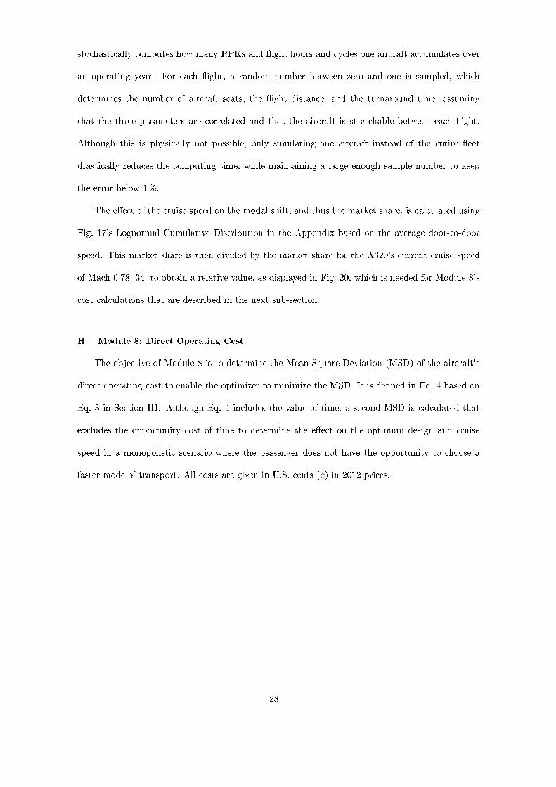
2. Including the Value of Time

As implied in the name and de�ned in Eq. 3 in Section III, MSD is the mean of the squares of

the DOC values. In order to make comparisons with the mean DOC values quoted in the previous

sub-section easier, Fig. 11 presents the square root of the MSD, but including the absolute instead

of the relative cost of time.

Fig. 11 System options MSD of direct operating cost (incl. value of time) vs. cruise speed.

If the value of time is included, Fig. 11 con�rms that the geared turbofan has the lowest DOC

of the �ve system options at a cruise speed of Mach 0.80 and that System Option 2 has an almost

identical operating cost to System Option 1, despite a 10% engine acquisition cost penalty imposed

on the three-shaft turbofan to account for the lighter but more complex design in comparison to

the two-shaft con�guration. Figure 11 also highlights the turboprop's narrow optimum cruise speed

range in comparison to the three turbofans and the open rotor.

Figure 12 compares the optimum system option designs, based on the minimum DOC (including

the relative value of time) at Mach 0.80 for System Options 1�3, Mach 0.72 for System Option 4, and

Mach 0.76 for System Option 5 to the actual DOC data of U.S. passenger airlines in the Year 2009 [17,

18]. The actual engine and airframe costs from 2009 have been blended together in Fig. 12 because

34

the data does not di�erentiate between the two. As the U.S. passenger airlines data also does not

separate the productivity cost from the rest and does not include market share and time costs, none

of these are shown in Fig. 12. Although the actual cost data is an average for all aircraft sizes

and ages operated by U.S. passenger airlines in 2009, the comparison between the predicted and

the actual DOC data nevertheless reveals that the costs estimates for 2030 are realistic, considering

that Table 9 shows that the aircraft acquisition costs are forecasted to rise to balance the high fuel

and CO2 cost estimates for 2030. The actual fuel cost in 2009 is signi�cantly less than forecasted

for 2030, because in addition to supplementary CO2 costs, the mean predicted oil price for 2030

(≈ 135 $/barrel in 2012 prices) is more than twice as high as the actual price in 2009 (≈ 63 $/barrel

in 2012 prices [17, 18]). This price increase between 2009 and 2030 does not translate into a similar

fuel and CO2 cost rise in Fig. 12 due to the signi�cantly improved fuel e�ciency highlighted in

Table 8. As the landing and navigation charges are dependent on the Operating Weight Empty

(OWE) which, according to Table 9, is predicted to reduce, Fig. 12 indicates that these are the only

costs that are expected to drop.

Fig. 12 Optimum system options (incl. value of time) vs. actual U.S. passenger airlines [17, 18]

direct operating cost breakdown.

Focusing on the �ve system options, Fig. 12 con�rms that the geared turbofan has the lowest

operating cost if the value of time is included. Nevertheless, Table 6 shows that the turboprop,

which has the highest operating cost, is only 3.4% more expensive. Even though System Option 2

has the most costly engine, Fig. 12 illustrates that this is over-compensated by the reduced fuel

consumption, making it slightly cheaper to operate than the two-shaft turbofan. However, System

35

Option 3 outperforms both in terms of cost e�ciency because the reduced engine weight and fuel

consumption also make the airframe lighter and therefore cheaper. Although the turboprop has the

lowest engine cost due to the reduced turbine entry temperature and thrust requirement, the lightest

and cheapest airframe and the highest fuel e�ciency, the low cruise speed imposes a signi�cant

productivity and time cost, making it the most expensive option. Despite not having such a large

time and productivity cost, System Option 5's high thrust and turbine entry temperature make the

engine the second most expensive to operate. The high engine mass also does not help in reducing

the airframe weight and hence its cost. Although the open rotor is more fuel-e�cient than the

geared turbofan, it has a higher fuel consumption than the turboprop due to the increased cruise

speed.

3. Excluding the Value of Time

As the cost of time drops linearly with an increase in cruise speed, Fig. 13 is a tilted version

of Fig. 11 in which the turboprop is the cheapest system option after being the most expensive in

Fig. 11. However, as indicated in Table 6, the geared turbofan only slips down one rank to second,

ahead of the open rotor and the two- and three-shaft turbofan.

Fig. 13 System options MSD of direct operating cost (excl. value of time) vs. cruise speed.

Figure 14 looks similar to Fig. 12, except that the cost of time is not included and that most of

the costs have decreased, except for a marginal rise in the productivity and market share costs due

to the reduced cruise speeds. While the turboprop's cruise velocity has only dropped by Mach 0.02,

the turbofans' have decreased by Mach 0.04 and the open rotor's by Mach 0.06 which explains their

36

more pronounced fuel cost saving. All system options have similar reductions in engine and airframe

costs, however, due to the lower airframe weight and thrust requirement. As all costs, except for

fuel and CO2, have changed by similar amounts, it is not surprising that the turboprop is now the

cheapest to operate without the cost of time. Similarly, the geared turbofan's lower engine and

airframe weight and cost and its productivity cost advantage outweigh the open rotor's superior

fuel e�ciency. This shows that the most fuel-e�cient option, the open rotor, is not automatically

the most cost-e�cient solution because of the relatively high engine and airframe costs.

Fig. 14 Optimum system options (excl. value of time) vs. actual U.S. passenger airlines [17, 18]

direct operating cost breakdown.

Table 7 shows that the√MSD and mean DOC values are almost identical, which explains why

both have the same optimum cruise speeds. The minor di�erence in cost is caused by the fact that,

despite the uniform uncertainty distributions,√MSD is skewed by the higher fuel and carbon cost

values due to the squaring, as Eqs. 5 and 6 demonstrate for imagined values of 1.0, 1.5 and 2.0:

√MSD =

√1

M

∑M

j=1y2j =

√1

3× (1.02 + 1.52 + 2.02) = 1.55 (5)

Mean DOC =1

M

∑M

j=1yj =

1

3× (1.0 + 1.5 + 2.0) = 1.50 (6)

This raises the question whether it was worthwhile determining the MSD when using a uniform

uncertainty distribution. The authors argue that it was, considering that the MSD provides a clear

link between the fuel and carbon price ranges speci�ed in Section I and the model, as well as a

baseline against which the mean DOC could be compared.

37

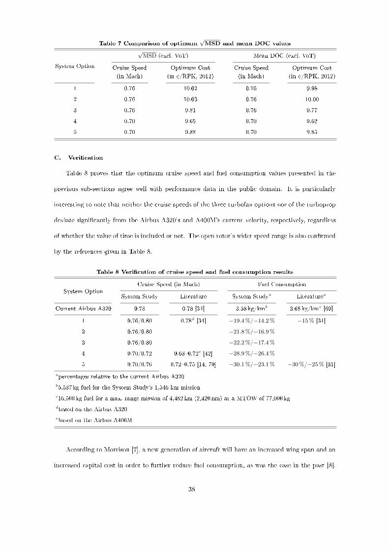
Table 7 Comparison of optimum√MSD and mean DOC values

√MSD (excl. VoT) Mean DOC (excl. VoT)

Cruise Speed Optimum Cost Cruise Speed Optimum CostSystem Option

(in Mach) (in ¢/RPK, 2012) (in Mach) (in ¢/RPK, 2012)

1 0.76 10.02 0.76 9.98

2 0.76 10.03 0.76 10.00

3 0.76 9.81 0.76 9.77

4 0.70 9.65 0.70 9.62

5 0.70 9.88 0.70 9.85

C. Veri�cation

Table 8 proves that the optimum cruise speed and fuel consumption values presented in the

previous sub-sections agree well with performance data in the public domain. It is particularly

interesting to note that neither the cruise speeds of the three turbofan options nor of the turboprop

deviate signi�cantly from the Airbus A320's and A400M's current velocity, respectively, regardless

of whether the value of time is included or not. The open rotor's wider speed range is also con�rmed

by the references given in Table 8.

Table 8 Veri�cation of cruise speed and fuel consumption results

Cruise Speed (in Mach) Fuel ConsumptionSystem Option

System Study Literature System Studya Literaturea

Current Airbus A320 0.78 0.78 [34] 3.58 kg/kmb 3.68 kg/kmc [69]

1 0.76/0.80 0.78d [34] −19.4 %/−14.2 % −15 % [31]

2 0.76/0.80 −21.8 %/−16.9 %

3 0.76/0.80 −22.2 %/−17.4 %

4 0.70/0.72 0.68�0.72e [42] −28.9 %/−26.4 %

5 0.70/0.76 0.72�0.75 [14, 70] −30.1 %/−23.1 % −30 %/−25 % [31]

apercentages relative to the current Airbus A320b5,537 kg fuel for the System Study's 1,546-km missionc16,500 kg fuel for a max. range mission of 4,482 km (2,420 nm) at a MTOW of 77,000 kgdbased on the Airbus A320ebased on the Airbus A400M

According to Morrison [7], a new generation of aircraft will have an increased wing span and an

increased capital cost in order to further reduce fuel consumption, as was the case in the past [8].

38

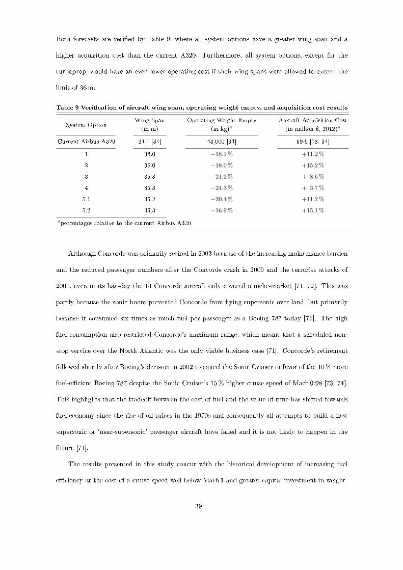
Both forecasts are veri�ed by Table 9, where all system options have a greater wing span and a

higher acquisition cost than the current A320. Furthermore, all system options, except for the

turboprop, would have an even lower operating cost if their wing spans were allowed to exceed the

limit of 36m.

Table 9 Veri�cation of aircraft wing span, operating weight empty, and acquisition cost results

Wing Span Operating Weight Empty Aircraft Acquisition CostSystem Option

(in m) (in kg)a (in million $, 2012)a

Current Airbus A320 34.1 [34] 43,000 [34] 69.6 [18, 34]

1 36.0 −18.1 % +11.2 %

2 36.0 −18.0 % +15.2 %

3 35.8 −21.2 % + 8.6 %

4 35.3 −24.3 % + 3.7 %

5.1 35.2 −20.4 % +11.2 %

5.2 35.3 −16.9 % +15.1 %

apercentages relative to the current Airbus A320

Although Concorde was primarily retired in 2003 because of the increasing maintenance burden

and the reduced passenger numbers after the Concorde crash in 2000 and the terrorist attacks of

2001, even in its hay-day the 14 Concorde aircraft only covered a niche-market [71, 72]. This was

partly because the sonic boom prevented Concorde from �ying supersonic over land, but primarily

because it consumed six times as much fuel per passenger as a Boeing 787 today [71]. The high

fuel consumption also restricted Concorde's maximum range, which meant that a scheduled non-

stop service over the North Atlantic was the only viable business case [71]. Concorde's retirement

followed shortly after Boeing's decision in 2002 to cancel the Sonic Cruiser in favor of the 10% more

fuel-e�cient Boeing 787 despite the Sonic Cruiser's 15% higher cruise speed of Mach 0.98 [73, 74].

This highlights that the tradeo� between the cost of fuel and the value of time has shifted towards

fuel economy since the rise of oil prices in the 1970s and consequently all attempts to build a new

supersonic or `near-supersonic' passenger aircraft have failed and it is not likely to happen in the

future [71].

The results presented in this study concur with the historical development of increasing fuel

e�ciency at the cost of a cruise speed well below Mach 1 and greater capital investment in weight-

39

and fuel-saving technologies like the geared turbofan and composite airframes. This development

is already taking place today, as Pratt & Whitney's geared turbofan is being installed on several

single-aisle aircraft and Rolls-Royce is pursuing a similar development [37, 75].

Morrison [7] also predicts that rising fuel prices will lead to a reduction in cruise speed, but this

can only by veri�ed by the results if the value of time is excluded. If the fuel and carbon prices

were to increase above the range assumed in this study, however, then the higher fuel costs will

have a greater leverage on the cruise speed than the value of time. Consequently, it would be more

likely that the turboprop would be the cheapest aircraft to operate, regardless of whether the value

of time is included or not. This would agree with Rolls-Royce's statement [33] that �there is very

sound argument to be made for the majority of the 150-seat market, which �ies mostly for less than

1.5 hours [being turboprop-powered]�.

VI. Conclusion

As outlined in Section I, the originality of this study lies in the holistic approach of combin-

ing system design engineering and performance simulation with economic forecasting, operational

research, robust design, and multi-objective optimization. This enabled �ve di�erent engine and

airframe system options, including the two- and three-shaft turbofan, the geared turbofan, the tur-

boprop, and the open rotor aircraft designs to be optimized in MATLAB in terms of direct operating

cost for a standard mission, so that a fair quantitative comparison could be made in light of uncertain

fuel and CO2 prices in 2030. Due to time constraints, neither a sensitivity study was carried out,

nor for example whether the value of time of business travelers would justify a supersonic business

jet.

The design variables optimized include the engine's turbine entry temperature, its overall pres-

sure ratio, and the airframe's wing span and mean chord length. In addition, the three turbofan

options' fan pressure ratio was varied, as well as the turboprop's and the open rotor's propeller di-

ameter and rotational tip speed. Although the e�ect of the cruise speed on the system performance

was also investigated, the designs were only optimized for one cruise velocity.

The cruise speed not only a�ects the fuel consumption, but also the productivity of the aircraft

40

�eet, the opportunity cost resulting from the Value of Time (VoT) of the passengers, and the

market share of the aircraft in comparison to other modes of transport. All these aspects are

therefore taken into account by the model, but not di�erent aircraft sizes, �ight pro�les, and annual

passenger numbers (i.e. demand).

The passenger VoT has a large e�ect on the tradeo� between the cost of fuel and the total cost

of time of the aircraft, crew, and passengers: while the geared turbofan cruising at Mach 0.80 is the

optimum design when the passenger VoT is taken into account, it is the turboprop at Mach 0.70

when the value of time is excluded for a monopolistic scenario in which the passenger does not have

the opportunity to select a faster mode of transport. This shows that the most fuel-e�cient option,

the open rotor, is not automatically the most cost-e�cient solution because of the relatively high

engine and airframe costs.

Appendix

In order to determine how the market share of the aircraft is a�ected by its cruise speed,

o�cial travel time data from airline websites was collected that o�ered transport services between

40 European city pairs. To account for actual door-to-door times, three hours were added to the

�ight times, assuming that it takes one hour to get to the airport, one hour to check in and board

the aircraft, and one hour to travel to the �nal destination [40]. Figure 15 shows these 40 door-

to-door times plotted against the direct distance between the city pairs. These data points were

then used to generate the linear regression line that is also displayed in Fig. 15. While the inverse

of the regression line's gradient re�ects today's average cruise speed of 812 km/h (≈ 500mph), the

intercept of 3 hours and 40 minutes is the sum of the regressed idle time of the �ights (40 minutes)

and the three hours added by the authors. The regression line forms the basis of the second graph

in Fig. 15, which shows how the average door-to-door speed increases with distance.

41

Fig. 15 Total �ight journey time vs. direct distance.

Figure 16 illustrates how the market share of the aircraft, the high-speed train, and the car

changes with distance, based on a diagram presented by Jenkinson et al. [55]. While the market share

graphs of the aircraft and the car were constructed using the Lognormal Cumulative Distribution

(LCD), the train curve simply represents the remaining market share. The distributions would

probably look very di�erent for city pairs without a high-speed train connection. By including high-

speed rail rather than other slower modes of transport that compete less with air travel, however,

a conservative estimate about the market share of the aircraft is being made.

Fig. 16 Aircraft, high-speed train, and car market share vs. direct distance (data based on

Ref. [55]).

The market share data shown in Fig. 16 was used in conjunction with the speed-distance rela-

tionship in Fig. 15 to derive how the aircraft's market share is related to its average door-to-door

speed. Rather than using Fig. 16's LCD based on distance, the aircraft's market share can also be

42

described by a LCD as function of the average door-to-door speed, as Fig. 17 indicates that the two

distributions overlap almost perfectly.

Fig. 17 Aircraft market share vs. average door-to-door speed.

Assuming that the market share of the aircraft is dependent on the average door-to-door speed,

the four graphs in Fig. 18 were created by �rst calculating the average door-to-door times for the

various cruise speeds and direct distances, and then using these in conjunction with Fig. 17's speed-

based LCD to obtain the respective market shares. For cruise speeds above 600 km/h (≈ 370mph),

Fig. 18 clearly shows that the aircraft becomes competitive at a direct travel distance of around

400 km (≈ 250mi) and reaches a market share above 90% at 1,000 km (≈ 620mi) almost regardless

of the cruise speed. Between 400 and 1,000 km, where the aircraft competes most with the other

forms of transport, however, the cruise speed does a�ect the market share.

Fig. 18 Impact of cruise speed on aircraft market share.

According to Airbus [19], 70% of single-aisle aircraft will �y 1,850 km (≈ 1,150mi) or less in

43

2028. This information, together with the assumption that no 150-seater �ight will be less than

250 km (≈ 150mi) but 5% will be less than 500 km, produced the LCD shown in Fig. 19. The

LCD was capped at a �ight distance of 3,000 nautical miles (≈ 5,550 km / 3,450mi) because that is

the likely design range for the next-generation 150-seater [64]. Based on 10,000 stochastic samples

of this distribution, the mean �ight distance is 1,546 km with a standard error of 10.2 km. The

standard error is a measure of the precision of the estimate and is de�ned as the standard deviation

of the distribution divided by the square root of the sample number [76]. To save computing time,

only the average �ight distance was used to �nd the optimum engine and airframe design.

Fig. 19 Single-aisle aircraft �ight distance distribution.

As Fig. 19 indicates that less than 40% of the single-aisle �ights are less than 1,000 km, Fig. 20

illustrates that the reduced market share in the 400�1,000 km segment only starts to a�ect the

cumulative market share of the aircraft signi�cantly if the cruise speed falls below 400 km/h. Here

the cumulative market share is expressed in relative passenger-kilometers, i.e. the RPKs �own at

the various speeds are divided by the RPKs �own at today's cruise speed of 812 km/h.

44

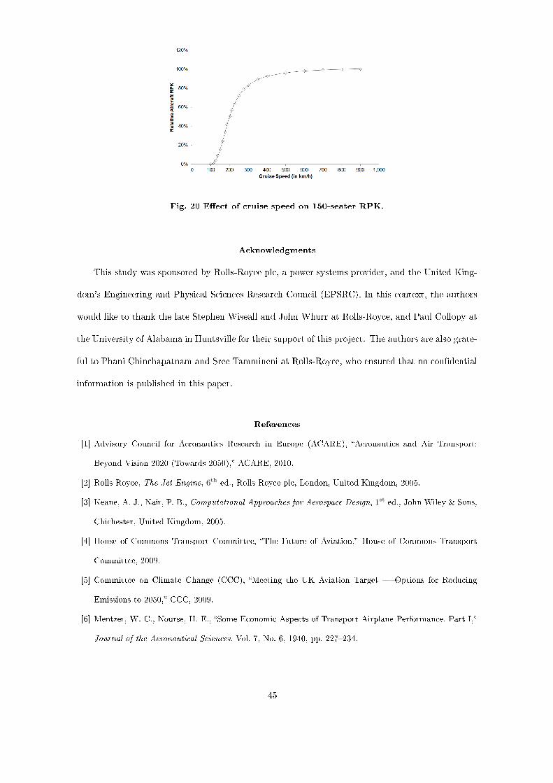
Fig. 20 E�ect of cruise speed on 150-seater RPK.

Acknowledgments

This study was sponsored by Rolls-Royce plc, a power systems provider, and the United King-

dom's Engineering and Physical Sciences Research Council (EPSRC). In this context, the authors

would like to thank the late Stephen Wiseall and John Whurr at Rolls-Royce, and Paul Collopy at

the University of Alabama in Huntsville for their support of this project. The authors are also grate-

ful to Phani Chinchapatnam and Sree Tammineni at Rolls-Royce, who ensured that no con�dential

information is published in this paper.

References

[1] Advisory Council for Aeronautics Research in Europe (ACARE), �Aeronautics and Air Transport:

Beyond Vision 2020 (Towards 2050),� ACARE, 2010.

[2] Rolls-Royce, The Jet Engine, 6th ed., Rolls-Royce plc, London, United Kingdom, 2005.

[3] Keane, A. J., Nair, P. B., Computational Approaches for Aerospace Design, 1st ed., John Wiley & Sons,

Chichester, United Kingdom, 2005.

[4] House of Commons Transport Committee, �The Future of Aviation,� House of Commons Transport

Committee, 2009.

[5] Committee on Climate Change (CCC), �Meeting the UK Aviation Target � Options for Reducing

Emissions to 2050,� CCC, 2009.

[6] Mentzer, W. C., Nourse, H. E., �Some Economic Aspects of Transport Airplane Performance. Part I,�

Journal of the Aeronautical Sciences, Vol. 7, No. 6, 1940, pp. 227�234.

45

[7] Morrison, S. A., �An Economic Analysis of Aircraft Design,� Journal of Transport Economics and

Policy, Vol. 18, No. 2, 1984, pp. 123�143.

[8] Lee, J. J., Lukachko, S. P., Waitz, I. A., Schafer, A., �Historical and Future Trends in Aircraft Per-

formance, Cost, and Emissions,� Annual Review of Energy and the Environment, Vol. 26, No. 1, 2001,

pp. 167�200.

[9] Antoine, N., Kroo, I., Willcox, K., Barter, G., �A Framework for Aircraft Conceptual Design and

Environmental Performance Studies,� 10 thAIAA/ISSMO Multidisciplinary Analysis and Optimization

Conference, Albany, New York, USA, 2004.

[10] Bower, G. C., Kroo, I. M., �Multi-Objective Aircraft Optimization for Minimum Cost and Emissions

over Speci�c Route Networks,� 26 thInternational Congress of the Aeronautical Sciences (ICAS), An-

chorage, Alaska, USA, 2008.

[11] Kernstine, K., Boling, B., Bortner, L., Hendricks, E., Mavris, D., �Designing for a Green Future: a

Uni�ed Aircraft Design Methodology,� Journal of Aircraft, Vol. 47, No. 5, 2010, pp. 1789�1797.

[12] Mavris, D. N., Mantis, G. C., Kirby, M. R., �Demonstration of a Probabilistic Technique for the Deter-

mination of Aircraft Economic Viability,� SAE Transactions, Vol. 106, No. 1, 1997, pp. 1704�1713.

[13] Ryerson, M. S., Hansen, M., �The Potential of Turboprops for Reducing Aviation Fuel Consumption,�

Transportation Research Part D: Transport and Environment, Vol. 15, No. 6, 2010, pp. 305�314.

[14] Guynn, M. D., Berton, J. J., Hendricks, E. S., Tong, M. T., Haller, W. J., �Initial Assessment of

Open Rotor Propulsion Applied to an Advanced Single-Aisle Aircraft,� 11 thAIAA Aviation Technology,

Integration, and Operations Conference (ATIO), Virginia Beach, Virginia, USA, 2011.

[15] Peters, A., �Assessment of Propfan Propulsion Systems for Reduced Environmental Impact,� M.Sc.

Thesis, Massachusetts Institute of Technology, Boston, Massachusetts, USA, 2010.

[16] Hendricks, E. S., Tong, M. T., �Performance and Weight Estimates for an Advanced Open Rotor En-

gine,� 48 thAIAA/ASME/SAE/ASEE Joint Propulsion Conference & Exhibit, Atlanta, Georgia, USA,

2012.

[17] Airlines for America (A4A), �A4A Passenger Airlines Cost Index Tables,� A4A [online], 2009, https:

//publications.airlines.org/CommerceProductDetail.aspx?Product=152 [revisited 30 April 2015].

[18] Bureau of Labor Statistics, �CPI In�ation Calculator,� United States Department of Labor [online],

2014, http://www.bls.gov/data/inflation_calculator.htm [revisited 30 April 2015].

[19] Airbus, �Global Market Forecast 2009�2028,� Airbus S.A.S., 2009.

[20] Bowler, T., �Falling Oil Prices: Who are the Winners and Losers?,� BBC News [online], 2015, http:

//www.bbc.com/news/business-29643612 [revisited 30 April 2015].

46

[21] Donovan, S., Petrenas, B., Leyland, G., Caldwell, S., Barker, A., �Price Forecasts for Transport Fuels

and Other Delivered Energy Forms,� Auckland Regional Council, 2009.

[22] BBC News, �Oil Hits $ 100 Barrel,� BBC News [online], 2008, http://news.bbc.co.uk/1/hi/business/

7083015.stm [revisited 30 April 2015].

[23] U.S. Energy Information Administration (EIA), �International Energy Outlook 2013,� EIA, 2013.

[24] Department of Energy & Climate Change (DECC), �DECC Fossil Fuel Price Projections,� DECC, 2013.

[25] European Central Bank (ECB), �Euro Foreign Exchange Reference Rates,� ECB [online], 2015, http:

//www.ecb.europa.eu/stats/exchange/eurofxref/html/index.en.html [revisited 30 April 2015].

[26] Scheelhaase, J. D., Grimme, W. G., �Emissions Trading for International Aviation � an Estimation of

the Economic Impact on Selected European Airlines,� Journal of Air Transport Management, Vol. 13,

No. 5, 2007, pp. 253�263.

[27] Anastasi, L., Dickinson, H., Kass, G., Smith, K., Stein, C., �Aviation and the Environment,� Parlia-

mentary O�ce of Science and Technology (POST), 2003.

[28] Department for Transport (DfT), �The Future of Air Transport,� DfT, 2003.

[29] Van Hasselt, M., Van der Zwan, F., Ghijs, S., Santema, S., �Developing a Strategic Framework for an

Airline Dealing with the EU Emission Trading Scheme,� 9 thAIAA Aviation Technology, Integration,

and Operations Conference (ATIO), Hilton Head, South Carolina, USA, 2009.

[30] The Guardian, �UK Calls for Cancelling of Carbon Permits to Revive EU Emissions

Trading,� The Guardian [online], 2014, http://www.theguardian.com/environment/2014/jul/

16/uk-calls-for-cancelling-of-carbon-permits-to-revive-eu-emissions-trading [revisited 30

April 2015].

[31] Parker, R., �From Blue Skies to Green Skies: Engine Technology to Reduce the Climate-Change Impacts

of Aviation,� Technology Analysis & Strategic Management, Vol. 21, No. 1, 2009, pp. 61�78.

[32] Riegler, C., Bichlmaier, C., �The Geared Turbofan Technology � Opportunities, Challenges and Readi-

ness Status,� 1 stCEAS European Air and Space Conference, Berlin, Germany, 2007.

[33] Daly, K., �Rolls-Royce Promotes Turboprop Solution for New Civil Airlin-

ers,� Flightglobal [online], 2008, http://www.flightglobal.com/news/articles/

rolls-royce-promotes-turboprop-solution-for-new-civil-224987/ [revisited 30 April 2015].

[34] Jackson, P. A., Jane's All the World's Aircraft 2006�2007, 97th ed., Jane's Information Group, Couls-

don, United Kingdom, 2006.

[35] Flightglobal, �Bristol Olympus,� Flightglobal [online], 1955, http://www.flightglobal.com/

pdfarchive/view/1955/1955%20-%201753.html [revisited 30 April 2015].

47

[36] Flightglobal, �R.B.211 Certi�cated,� Flightglobal [online], 1972, http://www.flightglobal.com/

pdfarchive/view/1972/1972%20-%200676.html [revisited 30 April 2015].

[37] Polek, G., �Pratt & Whitney Geared Turbofan Promises New Engine Dominance,� AIN-

online [online], 2013, http://www.ainonline.com/aviation-news/air-transport/2013-06-13/

pratt-whitney-geared-turbofan-promises-new-engine-dominance [revisited 30 April 2015].

[38] Flightglobal, �Development of the Turboprop,� Flightglobal [online], 1950, http://www.flightglobal.

com/pdfarchive/view/1950/1950%20-%202035.html [revisited 30 April 2015].

[39] Saravanamuttoo, H. I. H., �Modern Turboprop Engines,� Progress in Aerospace Sciences, Vol. 24, No. 3,

1987, pp. 225�248.

[40] Åkerman, J., �Sustainable Air Transport � on Track in 2050,� Transportation Research Part D: Trans-

port and Environment, Vol. 10, No. 2, 2005, pp. 111�126.

[41] European Aviation Safety Agency (EASA), �E.033 Europrop International GmbH TP400-D6 Engine,�

EASA, 2014.

[42] Jackson, P. A., Jane's All the World's Aircraft 2011�2012, 102nd ed., Jane's Information Group, Couls-

don, United Kingdom, 2011.

[43] McCormick, B. W., Aerodynamics, Aeronautics, and Flight Mechanics, 2nd ed., John Wiley & Sons,

Hoboken, New Jersey, USA, 1995.

[44] Flightglobal, �Whatever Happened to Propfans,� Flightglobal [online], 2007, http://www.

flightglobal.com/news/articles/whatever-happened-to-propfans-214520/ [revisited 30 April

2015].

[45] Warwick, G., �Noise Tests Keep Promise Of Open-Rotor Engines Alive,� Aviation Week, 2010.

[46] Schimming, P., �Counter Rotating Fans � an Aircraft Propulsion for the Future,� Journal of Thermal

Science, Vol. 12, No. 2, 2003, pp. 97�103.

[47] Bellocq, P., Sethi, V., Cerasi, L., Ahlefelder, S., Tantot, N., �Advanced Open Rotor Performance Mod-

elling for Multidisciplinary Optimization Assessments,� ASME Turbo Expo 2010: Power for Land, Sea

and Air, Glasgow, United Kingdom, 2010.

[48] European Commission, �valiDation of Radical Engine Architecture systeMs (DREAM),� Euro-

pean Commission [online], 2014, http://ec.europa.eu/research/transport/news/items/dream_ip_

encouraging_results_en.htm [revisited 30 April 2015].

[49] Collopy, P. D., �Economic-Based Distributed Optimal Design,� AIAA Space 2001 Conference and Ex-

position, Albuquerque, New Mexico, USA, 2001.

[50] Collopy, P. D., �Surplus Value in Propulsion System Design Optimization,�

48

33 rdAIAA/ASME/SAE/ASEE Joint Propulsion Conference & Exhibit, Seattle, Washington, USA,

1997.

[51] Hazelrigg, G. A., �A Framework for Decision-Based Engineering Design,� Journal of Mechanical Design,

Vol. 120, No. 4, 1998, pp. 653�658.

[52] Raymer, D. P., Aircraft Design: a Conceptual Approach, 4th ed., American Institute of Aeronautics and

Astronautics Inc., Reston, Virginia, USA, 2006.

[53] Vasigh, B., Fleming, K., Tacker, T., Introduction to Air Transport Economics: from Theory to Appli-

cations, 1st ed., Ashgate Publishing Limited, Farnham, United Kingdom, 2008.

[54] Doganis, R., Flying O� Course: the Economics of International Airlines, 3rd ed., Routledge, London,

United Kingdom, 2002.

[55] Jenkinson, L. R., Simpkin, P., Rhodes, D., Civil Jet Aircraft Design, 1st ed., Butterworth-Heinemann,

Oxford, United Kingdom, 1999.

[56] Cook, A., Tanner, G., �European Airline Delay Cost Reference Values,� University of Westminster,

London, United Kingdom, 2011.

[57] Institut du Transport Aérien (ITA), �Costs of Air Transport Delay in Europe,� ITA, 2000.

[58] Brons, M., Pels, E., Nijkamp, P., Rietveld, P., �Price Elasticities of Demand for Passenger Air Travel:

a Meta-Analysis,� Journal of Air Transport Management, Vol. 8, No. 3, 2002, pp. 165�175.

[59] EUROCONTROL, �Standard Inputs for EUROCONTROL Cost Bene�t Analyses Edition 4.0,� EU-

ROCONTROL, 2009.

[60] Trimble, S., �Analysis: Noise Goals in Sight for Open-Rotor Researchers,�

Flightglobal [online], 2014, http://www.flightglobal.com/news/articles/

analysis-noise-goals-in-sight-for-open-rotor-researchers-395804/ [revisited 30 April

2015].

[61] European Aviation Safety Agency (EASA), �E.069 International Aero Engines AG (IAE) V2500-A5 and

V2500-D5 Series Engines,� EASA, 2013.

[62] Wickerson, J., �Holistic Gas Turbine,� Rolls-Royce plc, 2008.

[63] Howe, D., Aircraft Conceptual Design Synthesis, 1st ed., Professional Engineering Publishing Limited,

London and Bury St. Edmunds, United Kingdom, 2000.

[64] Airbus, �Airbus UK / University of Bath Speci�cation for Aerospace Design Project 2007 � Low Fare

Airline Optimised Aircraft,� Airbus S.A.S., 2007.

[65] Mattingly, J. D., Heiser, W. H., Pratt, D. T., Aircraft Engine Design, 2nd ed., American Institute of

Aeronautics and Astronautics Inc., Reston, Virginia, USA, 2002.

49

[66] Lock, G. D., �Aircraft Propulsion,� University of Bath, 2006.

[67] Airbus, �Global Market Forecast 2011�2030,� Airbus S.A.S., 2011.

[68] Hooke, R., Jeeves, T. A., �Direct Search Solution of Numerical and Statistical Problems,� Journal of

the ACM (JACM), Vol. 8, No. 2, 1961, pp. 212�229.

[69] Airbus, �A320 Airplane Characteristics for Airport Planning,� Airbus S.A.S., 2011.

[70] Parker, R., Lathoud, M., �Green Aero-Engines: Technology to Mitigate Aviation Impact on Environ-

ment,� Proceedings of the Institution of Mechanical Engineers, Part C: Journal of Mechanical Engi-

neering Science, Vol. 224, No. 3, 2010, pp. 529�538.

[71] Calder, S., �Concorde and Supersonic Travel: the Days When the Sun Rose in the

West,� The Independent [online], 2013, http://www.independent.co.uk/travel/news-and-advice/

concorde-and-supersonic-travel-the-days-when-the-sun-rose-in-the-west-8888836.html [re-

visited 30 April 2015].

[72] BBC News, �Concorde Grounded for Good,� BBC News [online], 2003, http://news.bbc.co.uk/1/hi/

uk/2934257.stm [revisited 30 April 2015].

[73] Fagan, M., �Boeing Axes Sonic Cruiser as Airlines Lose Interest,� The

Telegraph [online], 2002, http://www.telegraph.co.uk/finance/2837367/

Boeing-axes-Sonic-Cruiser-as-airlines-lose-interest.html [revisited 30 April 2015].

[74] Norris, G., �Sonic Cruiser is Dead � Long Live Super E�cient,� Flightglobal [online], 2003, http://www.

flightglobal.com/news/articles/sonic-cruiser-is-dead-long-live-super-efficient-159915/

[revisited 30 April 2015].

[75] Krauskopf, L., �GE Exec Says Avoided Geared Design in Jet Engine Battle with

Pratt,� Thomson Reuters [online], 2014, http://www.reuters.com/article/2014/09/15/

us-general-electric-united-tech-engine-idUSKBN0HA2H620140915 [revisited 30 April 2015].

[76] Montgomery, D. C., Runger, G. C., Applied Statistics and Probability for Engineers, 3rd ed., John Wiley

& Sons, Danvers, Massachusetts, USA, 2003.

50