ROBUST ESTIMATION FOR DIFFERENTIAL EQUATIONS, TIME … · ROBUST ESTIMATION FOR DIFFERENTIAL EQUATIONS, ... Robust Estimation for Differential Equations, Time Series ... staff and

ROBUST ESTIMATION FOR DIFFERENTIAL

EQUATIONS, TIME SERIES ANALYSIS ON CLIMATE

CHANGE AND MCMC SIMULATION OF

DURATION-OF-LOAD PROBLEM

by

Jia Xu

Master of Science, Zhejiang University, 2006-2008

Bachelor of Science, Zhejiang University, 2002-2006

THESIS SUBMITTED IN PARTIAL FULFILLMENT

OF THE REQUIREMENTS FOR THE DEGREE OF

MASTER OF SCIENCE

IN THE DEPARTMENT

OF

STATISTICS AND ACTUARIAL SCIENCE

c© Jia Xu 2010

SIMON FRASER UNIVERSITY

Summer 2010All rights reserved. However, in accordance with the Copyright Act of Canada,this work may be reproduced, without authorization, under the conditions forFair Dealing. Therefore, limited reproduction of this work for the purposes ofprivate study, research, criticism, review, and news reporting is likely to be

in accordance with the law, particularly if cited appropriately.

APPROVAL

Name: Jia Xu

Degree: Master of Science

Title of Thesis: Robust Estimation for Differential Equations, Time Series

Analysis on Climate Change and MCMC Simulation of Duration-

of-load Problem

Examining Committee: Dr. Derek Bingham

Associate Professor of Statistics and Actuarial Science (Chair)

Dr. Jiguo Cao

Supervisor

Assistant Professor of Statistics and Actuarial

Science

Dr. Leilei Zeng

Assistant Professor of Statistics and Actuarial

Science

Faculty of Health Sciences

Dr. Zhaosong Lu

External Examiner

Assistant Professor of Mathematics

Date Approved:

ii

Abstract

Usually we need to estimate the unknown parameters of Ordinary Differential Equations

based on given data. We propose a robust method in which the parameters are estimated in

two levels of optimization. Simulation studies show that the robust method gives satisfac-

tory results. We also apply the robust method to a real ecological data set.

Standard normal homogeneity test and Yao and Davis’ test aretwo widely used meth-

ods in climate study. We generate data from four models and examine whether these two

tests are sensitive to different models. We also apply thesemethods to the climate data of

Barkerville, BC.

Duration-of-load problem is of great importance in wood engineering. We present lit-

erature reviews of three papers in this field. Then we conductMarkov Chain Monte Carlo

simulation to explore the empirical probability densitiesof the break time of lumbers under

different models.

Keywords: ordinary differential equation, generalized profiling method, robust method,

climate study, standard normal homogeneity test, Yao and Davis’ test, Markov Chain Monte

Carlo, MCMC, Duration-of-load

iii

Acknowledgments

I give my enduring gratitude to the faculty, staff and my fellow students at the SFU De-

partment of Statistics and Actuarial Science, who have combined to create a stimulating

environment for research in my field. I owe particular thanksto Dr. Jiguo Cao, who taught

me how to question more deeply and solve practical problems.

I thank Dr. Derek Bingham, Dr. Leilei Zeng and Dr. Zhaosong Lufor spending time

reading my thesis and also giving valuable suggestions. I also thank them for supervising

my defense as committee members.

I thank Dr. Peter Guttorp from University of Washington for supervising the climate

study project and giving valuable ideas on how to conduct theanalysis for the climate data

of Barkerville. I thank Dr. Charmaine Dean for providing thefund for the climate study. I

also thank Mr. Paul Whitfield from SFU for providing the climate data of Barkerville and

giving useful suggestions on the interpretation of the climate data set.

I also thank my fellow student Jing Cai for programming in Matlab and Winbugs for

MCMC simulation of the Duration-of-load problem and generating Figure 11.1, Figure

11.2, Table 12.1 and Table 12.2.

iv

Contents

Approval ii

Abstract iii

Acknowledgments iv

Contents v

List of Figures viii

List of Tables x

1 Introduction 1

1.1 Overview . . . . . . . . . . . . . . . . . . . . . . . . . . . . . . . . . . . 1

1.2 One Example . . . . . . . . . . . . . . . . . . . . . . . . . . . . . . . . . 2

1.3 Generalized Profiling Method . . . . . . . . . . . . . . . . . . . . . . .. . 3

1.3.1 ODE Model with Single Component . . . . . . . . . . . . . . . . . 3

1.3.2 ODE Model with Multiple Components . . . . . . . . . . . . . . . 6

1.3.3 Selection of the Smoothing Parameter . . . . . . . . . . . . . .. . 7

1.3.4 B-spline Basis . . . . . . . . . . . . . . . . . . . . . . . . . . . . 7

2 Robust Method 10

2.1 ODE Model with Single Component . . . . . . . . . . . . . . . . . . . . .11

2.2 ODE Model with Multiple Components . . . . . . . . . . . . . . . . . .. 12

2.3 Selection of the Smoothing Parameter . . . . . . . . . . . . . . . .. . . . 12

2.4 Relative Efficiency . . . . . . . . . . . . . . . . . . . . . . . . . . . . . . 13

v

CONTENTS vi

2.5 Numerical Algorithms . . . . . . . . . . . . . . . . . . . . . . . . . . . . 13

2.5.1 Simpson’s Rule . . . . . . . . . . . . . . . . . . . . . . . . . . . . 13

2.5.2 Computation of Gradients . . . . . . . . . . . . . . . . . . . . . . 13

2.5.3 Sandwich Method . . . . . . . . . . . . . . . . . . . . . . . . . . 14

3 Simulation and Application 17

3.1 Simulation . . . . . . . . . . . . . . . . . . . . . . . . . . . . . . . . . . . 17

3.1.1 Linear ODE . . . . . . . . . . . . . . . . . . . . . . . . . . . . . . 19

3.1.2 FitzHugh-Nagumo Equations . . . . . . . . . . . . . . . . . . . . 24

3.2 Application to Predator-Prey Model . . . . . . . . . . . . . . . . .. . . . 30

4 Conclusion and Discussion 35

4.1 Conclusion . . . . . . . . . . . . . . . . . . . . . . . . . . . . . . . . . . 35

4.2 Discussion . . . . . . . . . . . . . . . . . . . . . . . . . . . . . . . . . . . 36

5 Homogenization Tests of Climate Series 37

5.1 Standard Normal Homogeneity Test . . . . . . . . . . . . . . . . . . .. . 37

5.2 Yao and Davis’ Test . . . . . . . . . . . . . . . . . . . . . . . . . . . . . . 39

5.3 Linear Trend . . . . . . . . . . . . . . . . . . . . . . . . . . . . . . . . . 39

5.4 Permutation Method . . . . . . . . . . . . . . . . . . . . . . . . . . . . . 41

6 Robustness of Homogenization Tests 42

6.1 Thick-tailed Distributions . . . . . . . . . . . . . . . . . . . . . . .. . . . 43

6.2 Autoregressive Memory . . . . . . . . . . . . . . . . . . . . . . . . . . . .48

6.3 Long-term Memory . . . . . . . . . . . . . . . . . . . . . . . . . . . . . . 48

7 Application to Barkerville, BC 51

7.1 Background of the Data . . . . . . . . . . . . . . . . . . . . . . . . . . . . 51

7.2 Conclusion . . . . . . . . . . . . . . . . . . . . . . . . . . . . . . . . . . 58

8 Discussion 60

8.1 Lowess . . . . . . . . . . . . . . . . . . . . . . . . . . . . . . . . . . . . 60

8.2 Multiple Jumps . . . . . . . . . . . . . . . . . . . . . . . . . . . . . . . . 60

CONTENTS vii

9 Literature Review of DOL Problem 63

9.1 Load-Duration Effects in Western Hemlock Lumber . . . . . .. . . . . . . 63

9.2 Probabilistic Modeling of Duration of Load Effects in Timber Structures . . 65

9.3 Duration of Load Effects And Reliability Based Design . .. . . . . . . . . 66

10 Markov Chain Monte Carlo 70

11 Simulation 72

11.1 Models . . . . . . . . . . . . . . . . . . . . . . . . . . . . . . . . . . . . 72

11.2 MCMC . . . . . . . . . . . . . . . . . . . . . . . . . . . . . . . . . . . . 73

12 Conclusion and Discussion 76

12.1 Conclusion . . . . . . . . . . . . . . . . . . . . . . . . . . . . . . . . . . 76

12.2 Discussion . . . . . . . . . . . . . . . . . . . . . . . . . . . . . . . . . . . 76

Appendix A: Selection of Matlab code for Chapter 3 79

Appendix B: Selection of Matlab code for Chapter 6 91

Appendix C: Selection of Winbugs code for Chapter 11 94

Bibliography 95

List of Figures

1.1 The numeric solutions of the predator-prey ODE (1.1) using the generalized

profiling parameter estimates and the parameter values given in Fussmann

et al. (2000). Observed experimental data are from Yoshida et al. (2003;

Fig. 2), with dilution ratesδ = 0.68day−1. The unit ofChlorella and

Brachionusis µmolL−1, and the unit of time is day. . . . . . . . . . . . . 4

1.2 Example of B-spline basis functions. . . . . . . . . . . . . . . . .. . . . . 8

2.1 The Huber functionρκ(r) and the first derivativedρκ/dr. . . . . . . . . . . 11

3.1 The PDF and CDF of Pareto(υ = 3,ξ = 1.5). . . . . . . . . . . . . . . . . 18

3.2 The simulated data from the linear ODE with 10 outliers added. The solid

line is the numerical solution to the linear ODE, and the outliers are marked

with circles. . . . . . . . . . . . . . . . . . . . . . . . . . . . . . . . . . . 21

3.3 The simulated data from the FitzHugh-Nagumo ODEs with 20outliers

added. The solid line is the numerical solution to the FitzHugh-Nagumo

ODEs, and the outliers are marked with circles. . . . . . . . . . . .. . . . 26

3.4 Solutions to the predator-prey ODEs (1.1) using the parameter values as

robust estimates, generalized profiling estimates and those in Fussmann et

al. (2000). Observed experimental data are from Yoshida et al. (2003; Fig.

2), with dilution ratesδ = 0.68day−1. The circle indicates the outlier iden-

tified by robust method. The unit ofChlorellaandBrachionusis µmolL−1,

and the unit of time is day. . . . . . . . . . . . . . . . . . . . . . . . . . . 33

6.1 Power curves of the difference version of SNHT . . . . . . . . .. . . . . . 44

6.2 Power curves of the ratio version of SNHT . . . . . . . . . . . . . .. . . . 45

viii

LIST OF FIGURES ix

6.3 Power curves of Yao & Davis’ method . . . . . . . . . . . . . . . . . . .. 46

6.4 The first panel shows an i.i.d.t(3) sequence with a jump=10 att = 500 and

the second panel shows the exponential of the sequence. . . . .. . . . . . 47

6.5 One simulated long-term memory series and its autocorrelation function

with d = 0.25. . . . . . . . . . . . . . . . . . . . . . . . . . . . . . . . . . 49

7.1 Temperature series of Barkerville . . . . . . . . . . . . . . . . . .. . . . . 52

7.2 Precipitation series of Barkerville . . . . . . . . . . . . . . . .. . . . . . 53

7.3 Histograms of detected jumps and jump times using different replacement

values with SNHT for temperature . . . . . . . . . . . . . . . . . . . . . . 54


values with Yao & Davis’ method for temperature . . . . . . . . . . .. . . 55


values with SNHT for precipitation . . . . . . . . . . . . . . . . . . . . .. 56

7.6 ACF of the modified Barkerville series . . . . . . . . . . . . . . . .. . . . 57

7.7 The result of SNHT: dash lines denote the 95% critical values. Replace

missing values with seasonal average. Use 95% critical value of LTM(0.127)

for temperature and 95% critical value of LTM(0.066) for precipitation.

There is a relocation in May, 1975(t = 1049) which may cause the last

jump of the precipitation. . . . . . . . . . . . . . . . . . . . . . . . . . . . 59

7.8 Yao & Davis’ method: the 95% critical value of LTM(0.127)is far above

the dots (about 5.7). . . . . . . . . . . . . . . . . . . . . . . . . . . . . . . 59

8.1 Lowess. The span = 10% of the sample size. . . . . . . . . . . . . . .. . . 61

8.2 Scatterplot of the differences between the estimated and the true jump times

(which can be positive or negtive). X-axis is for the first jump and Y-axis

for the second jump. The first five graphs at the first row are forjump =

0.1, 0.2, 0.3, 0.4, 0.5, etc. Each graph involves 1000 points. . . . . . . . . . 62

11.1 PDFs of break time for different models, different values ofk and different

scenarios when the data is generated from Madison model. . . .. . . . . . 75

11.2 PDFs of break time for different models, different values ofk and different

scenarios when the data is generated from EDRM model. . . . . . .. . . . 75

List of Tables

3.1 The biases, standard deviations (SDs), and root mean squared errors (RM-

SEs) of parameter estimates on 100 simulation replicates using the robust

method and the generalized profiling (GP) method. The true values of pa-

rameters areα1 = 3, andα2 = 10 . . . . . . . . . . . . . . . . . . . . . . . 22

3.2 The means and standard deviations (SDs) for the standarderror estimates

using the sandwich method over 100 simulation replicates. “Sample" rep-

resents the sample SDs of the parameter estimates. “CP" stands for the

coverage probabilities of the 95% confidence intervals for the parameters. . 25

3.3 The biases, standard deviations (SDs), and root mean squared errors (RM-

SEs) of parameter estimates on 100 simulation replicates using the robust

method and the generalized profiling (GP) method. The tuningparameter

in the Huber function,κ = 0.732σe, 0.982σe, 1.345σe , which correspond

to 85%, 90%, 95% asymptotic efficiency at the normal distribution. . . . . . 27

3.4 The means and standard deviations (SDs) for the standarderror estimates

using the sandwich method over 100 simulation replicates. “Sample" rep-

resents the sample SDs of the parameter estimates. “CP" stands for the

coverage probabilities of the 95% confidence intervals for the parameters. . 31

3.5 Parameter estimates and the standard errors (SEs) for the Predator-Prey

ODE model (1.1) from the real ecological data. MSE is defined as the

mean squared errors of the ODE solutions to the data excluding outliers.

As a comparison, we also give the parameter values given in Fussmann et

al. (2000) and the generalized profiling estimates. . . . . . . .. . . . . . . 32

x

LIST OF TABLES xi

6.1 95% critical values for different methods and models. SNHT diff. means

the difference version of SNTH (5.2) and SNHT ratio means theratio ver-

sion of SNHT (5.1). Yao & Davis’ means Yao & Davis’ method. . . .. . . 43

7.1 Estimate of the LTM parameterd and its 95% CI . . . . . . . . . . . . . . 58

12.1 Mean and standard deviation (SD) for each distributionwhen the data is

generated from Madison model. . . . . . . . . . . . . . . . . . . . . . . . 77

12.2 Mean and standard deviation (SD) for each distributionwhen the data is

generated from EDRM. . . . . . . . . . . . . . . . . . . . . . . . . . . . . 77

Chapter 1

Introduction

1.1 Overview

Ordinary Differential Equations (ODEs) are widely used in Biology, Economics, Finance

and other fields. The range of applications in Economics includes trade cycles, economic

chaos, urban pattern formation and economic growth (Zhang 2005). The stochastic version

of ODE - Stochastic Differential Equations (SDEs), are now heavily used in Financial En-

gineering, such as derivative pricing and risk management (Oksendal 2003). Probably the

most popular application of ODEs is in Biology, including population growth, administra-

tion of drugs, cell division and predator-prey models (Jones and Sleeman 2003).

In practice, unknown parameters are usually involved in theODEs. Given the data

available, we need to estimate the values of these parameters. If the ODEs can be solved

analytically, then the problem is relatively easy. However, it is not always the case. Actu-

ally in rear cases we can obtain the explicit expression of the ODEs. The first step is thus

to solve the ODEs numerically, and then use methods such as nonlinear, maximum likeli-

hood or Bayesian methods to approximate the parameters. Thedisadvantage of nonlinear

and maximum likelihood methods is that the result is very sensitive to the starting values

because usually there exist multiple local optimizers. Although Bayesian method can over-

come this problem, it is computationally extensive in most cases. Generalized profiling

method, which is designed as an alternative to the above methods, shows more popularity

recently (Ramsay and Silverman 2005). This method can not only effectively estimate the

parameters in ODEs but also prevent over-fitting of the modelby using a roughness penalty.

1

CHAPTER 1. INTRODUCTION 2

Usually the data we have is not perfect. There may exist outliers. A not-so-formal

approach is to plot the data and see if there are any unusual points. This is a useful method

because sometimes common sense will tell the obvious outliers from others. However,

we need a systematic method to deal with the outliers. Maronna et al. (2006) discuss the

robust method in detail. In this thesis we combine the robustmethod and the generalized

profiling method to proposal a new approach to deal with the parameter estimation problem

for ODEs.

1.2 One Example

The robust method for estimating ODE parameters is motivated by a predator-prey dy-

namic system described in Fussmann et al. (2000). An aquaticlaboratory community

containing two microbial species whose dynamic behavior isstudied by Fussmann et al.

(2000), Shertzer et al. (2002) and Yoshida et al. (2003). Thesystem is a nutrient-based

predator-prey food chain, in which unicellular green algae, Chlorella vulgaris, are eaten

by planktonic rotifers,Brachionus calyciflorus. The growth ofChlorella is also limited

by the supply of nitrogen.Chlorella andBrachionusare grown together in replicated, ex-

perimental flow-through cultures, called chemostats. Nitrogen continuously flows into the

system with concentrationN∗ at the dilution rateδ, and all variables are removed from the

chemostats at the same rateδ. Fussmann et al. (2000) mathematically model the system

using a set of nonlinear ODEs, coupled by consumer-resourceinteractions between the

planktonic rotifers, green algae, and the nitrogen resource:

dNdt

= δ(N∗−N)−FC(N)C

dCdt

= FC(N)C−FB(C)B/ε−δC

dRdt

= FB(C)R− (δ+m+α)R

dBdt

= FB(C)R− (δ+m)B (1.1)

whereN, C, R, B are the concentrations of nitrogen,Chlorella, reproducingBrachionus,

and totalBrachionus, respectively,FC(N) = bCN/(kC+N), FB(C) = bBC/(kB+C) are two

functional responses (withbC andbB the maximum birth rates ofChlorellaandBrachionus;


kC and kB the half-saturation constants ofChlorella and Brachionus), and ε, α, and m

are the assimilation efficiency, the decay of fecundity, andthe mortality ofBrachionus,

respectively.

The above dynamic model correctly predicts three qualitative types of dynamic be-

havior of the experimental system: the predator and prey coexist at an equilibrium at low

nutrient supply (smallδ or smallN∗); the system switches to a limit cycle when increasing

nutrient supply (increasingδ or N∗); very high nutrient supply leads to extreme oscillations

that cause the extinction of the predator or both the predator and the prey. However, Fuss-

mann et al. (2000) point out that their model performs poorlyat predicting quantitative

aspects of the experimental predator-prey dynamics because of the lack of knowledge on

the parameter values. Cao et al. (2008) improve the fitting ofthe ODE solution to the real

data by estimating the ODE parameters using the generalizedprofiling method.

Figure 1.1 displays the ODE solutions using the generalizedprofiling estimates and

the parameter values given in Fussmann et al. (2000). The generalized profiling method

clearly makes the ODE solutions fit the data better, which is agood validation for the ODE

model. However, one data point (marked with a circle in Figure 1.1) is too high for the

cyclic trend of the concentration of Brachionus, and may be an outlier, but the generalized

profiling method does not consider this outlier problem. Ourrobust method should further

improve the fitting of the ODE model by downweighting the impact of outliers.

1.3 Generalized Profiling Method

In this chapter we introduce a powerful method for approximating discrete data by a func-

tion - generalized profiling method (Ramsay and Silverman 2005). The key feture of this

method is the use of a roughness penalty.

1.3.1 ODE Model with Single Component

For simplicity, suppose the ODE only involves one component:

dxdt

= f (x|θ) (1.2)

whereθ is the parameter vector andx= x(t) is the dynamic process over timet.


4 6 8 10 12 14 160

20

40

60

80

Chl

orel

la

4 6 8 10 12 14 160

2

4

6

8

10

12

Time

Bra

chio

nus

DataFussmann et al. (2000)Generalized Profiling

DataFussmann et al. (2000)Generalized ProfilingPossible Outlier

Figure 1.1: The numeric solutions of the predator-prey ODE (1.1) using the generalized

profiling parameter estimates and the parameter values given in Fussmann et al. (2000).

Observed experimental data are from Yoshida et al. (2003; Fig. 2), with dilution rates

δ = 0.68day−1. The unit ofChlorella andBrachionusis µmolL−1, and the unit of time is

day.


We approximatex(t) by a linear combination of basis functions:

x(t) =K

∑k=1

ckφk(t) = cTφ(t) (1.3)

whereφk are basis functions andck are coefficients. In practice, the basis functions can be

Fourier basis, B-spline basis, wavelets and so on. We use B-spline basis because they can

accommodate the discontinuities by using multiple knots tothe time points (Ramsay and

Silverman 2005). Moreover, B-spline basis functions have aproperty called the compact

support property, which means that they are only positive over a short subinterval and zero

elsewhere. The compact support property makes the computation more efficient (More will

be covered in Section 1.3.4).

Let Y = (y1, . . . ,yn) be the observations of the dynamic process at timest1, . . . , tn. Gen-

eralized profiling method involves two steps. Theinner-optimizationminimizes

G(c|θ) =n

∑i=1

[yi −x(ti)]2+λ

∫ tn

t1[Lx(t)]2dt (1.4)

wheren

∑i=1

[yi −x(ti)]2 (1.5)

is just the sum of squares of residuals, which is equivalent to the log-likelihood under

normal assumption, and ∫ tn

t1[Lx(t)]2dt (1.6)

is defined as thepenaltyterm, which is used to control the roughness ofx(t). For instance,

operatorL can be

Lx=d2xdt2

(1.7)

if one wants to control the curvature of the functionx(t). Alternatively, we can use

Lx=dxdt

− f (x|θ) (1.8)

which serves as a measure of the deviation ofx(t) from the ODE (1.2).

λ is called thesmoothing parameter, which is a trade-off between fitting to data and

maintaining fidelity to the ODE model. There are two extreme cases: ifλ = 0, we place

total emphasis on fitting to data and the result is the same as that of least squares method;


if λ → ∞, we place total emphasis onx(t) maintaining fidelity to the ODE model. After the

inner-optimization,c or x= cTφ(t) is a function ofθ, whereT means transpose of a matrix.

Theouter-optimizationminimizes

H(θ) =n

∑i=1

[yi − c(θ)Tφ(ti)]2 (1.9)

which gives the final estimates of the parameters.

1.3.2 ODE Model with Multiple Components

In practice, there are often more than one component in the ODE model. Moreover, obser-

vations for some components may not exist or impossible to observe. Suppose we haveS

components (Ramsay and Silverman 2005):

dxℓdt

= fℓ(X|θ), ℓ= 1, . . . ,S (1.10)

whereX(t) = (x1(t), . . . ,xS(t))T. With no loss of generality, suppose only the firstM com-

ponents are observed, whereM ≤ S. Denotey j(ti j ) as the observation for thej-th compo-

nent at timeti j , i = 1, . . . ,n j , j = 1, . . . ,M . Again we express each component by a linear

combination of basis functions:

xℓ(t) = cTℓ φℓ(t), ℓ= 1, . . . ,S (1.11)

whereφℓ can be different basis systems for differentℓ. Thus, in the inner-optimization, we

minimize

G(c|θ) =M

∑j=1

ω j

n j

∑i=1

[y j(ti j )−x j(ti j )]2+

S

∑ℓ=1

λℓωℓ

∫ tn

t1[Lℓxℓ(t)]

2dt (1.12)

where

c= (cT1 , . . . ,c

TS)

T , Lℓxℓ =dxℓdt

− f (X|θ) (1.13)

andωℓ is the weight placed on componentxℓ, which can be chosen as the inverse of variance

of observations forxℓ. In the outer-optimization we minimizes

H(θ) =M

∑j=1

ω j

n j

∑i=1

[y j(ti j )− c j(θ)Tφ j(ti j )]2 (1.14)


1.3.3 Selection of the Smoothing Parameter

One problem is how to choose the value ofλ. One systematic method is calledcross-

validation (Ramsay and Silverman 2005). The basic idea is that for each value ofλ, we

leave one observation out and fit the model using the remaining part of the data, and then

estimate the fitted value for the observation left out. The procedure is repeated for each

observation in turn. Then we calculate thecross-validated error sum of squares, that is, the

resulting error sum of squares of all observations. We choose the value ofλ which mini-

mizes the cross-validated error sum of squares. However, this method is computationally

intensive (Ramsay and Silverman 2005).

In practice, we try a group of different values forλ and choose the one that minimizes

F(λ) =M

∑j=1

ω j

n j

∑i=1

[y j(ti j )−sj(ti j |θ(λ))]2 (1.15)

wheresj(ti j |θ(λ)) is the ODE solution at timeti j with the parameter estimateθ for the jth

component.

1.3.4 B-spline Basis

Spline functions are the most common choice of approximation system for non-periodic

functional data. To define a spline over an interval, first we divide the interval intoL subin-

tervals separated by breakpoints. The termbreakpointsrefers to the unique knots, while

the termknotsrefers to the sequence of values at breakpoints, where some breakpoints can

be associated with multiple knots. Over each interval, a spline is a polynomial of order

m. Theorder of a polynomial is the number of constants required to define it. Adjacent

polynomials join up smoothly at the breakpoint which separates them, so that the function

values are equal at their junction. Moreover, derivatives up to orderm−2 must also match

up at these junctions. The total number of degrees of freedomin the fit thus equals the order

of the polynomials plus the the number of interior breakpoints, that is,m+L−1 (Ramsay

and Silverman 2005).

The B-spline basis system developed by de Boor (2001) is the most popular one. The

property that an orderm B-spline basis function is positive over no more thanm intervals,


0 1 2 3 4 5 6 7 8 9 100

0.1

0.2

0.3

0.4

0.5

0.6

0.7

0.8

0.9

1

t

φ(t

)

B−spline basis, no. of basis functions = 15, order = 6

Figure 1.2: Example of B-spline basis functions.


and that these are adjacent, is called thecompact support property, and is of the greatest

importance for efficient computation. We use B-spline basisalso because they can ac-

commodate the discontinuities by using multiple knots to the breakpoints (Ramsay and

Silverman 2005). Figure 1.2 shows one example of B-spline basis functions with order 6.

Chapter 2

Robust Method

There are several versions of definition for robustness. In this chapter,robustnessrefers to

the notion of robust estimation with respect to outliers, that is, estimation is not sensitive to

outliers.

As long as there are no outliers in the data, generalized profiling method is a good

choice for parameter estimation. In practice, however, data collection sometimes involves

some errors. Obvious outliers can be detected solely by plotting the data. For example, the

height of a person is never negative, so if there is a negativevalue in the graph of the height

data, we can find and delete it with no doubt. But some outliersare not so easy to find out

just by looking at the graph. Plus, we need a systematic way toaddress the outlier problem.

Thus, we propose the robust method in this chapter.

Firstly we introduce the family ofHuber functions (Maronna et al. 2006):

ρκ(r) =

{r2 if |r| ≤ κ2κ|r|−κ2 if |r|> κ

(2.1)

whereκ > 0 is the cutoff of the Huber functions.

Half of its derivative is

12

ρ′κ(r) =

r if |r| ≤ κ

sign(r)κ if |r|> κ(2.2)

intuitively, the above function does nothing to the valuer if |r| ≤ κ; however, if|r| > κ, it

’pulls’ the valuer to κ or−κ, depending on the sign ofr. Figure 2.1 displays one example

of the Huber function and its first derivative.

10

CHAPTER 2. ROBUST METHOD 11

−3 −2 −k 0 k 2 30

2

4

6

r

ρ(r)

−3 −2 −k 0 k 2 3−4

−2

0

2

4

r

dρ/d

r

Figure 2.1: The Huber functionρκ(r) and the first derivativedρκ/dr.

2.1 ODE Model with Single Component

Firstly we are looking atdxdt

= f (x|θ) (2.3)

Now instead of using (1.4) in the inner-optimization, we minimize

G(c|θ) =n

∑i=1

ρκ[yi −x(ti)]+λ∫ tn

t1[Lx(t)]2dt (2.4)

where

x(t) = cTφ(t), Lx=dxdt

− f (x|θ) (2.5)

and similarly in the outer-optimization, we minimize

H(θ) =n

∑i=1

ρκ[yi − c(θ)Tφ(ti)] (2.6)


2.2 ODE Model with Multiple Components

As to the multiple components case,

dxℓdt

= fℓ(X|θ), ℓ= 1, . . . ,S (2.7)

whereX(t) = (x1(t), . . . ,xS(t))T. With no loss of generality, suppose only the firstM com-

ponents are observed, whereM ≤ S. The inner-optimization changes to

G(c|θ) =M

∑j=1

ω j

n j

∑i=1

ρκ j [y j(ti j )−x j(ti j )]+S

∑ℓ=1

λℓωℓ

∫ tn

t1[Lℓxℓ(t)]

2dt (2.8)

wherey j(ti j ) is the observation for thej-th component at timeti j , i = 1, . . . ,n j , j = 1, . . . ,M

and

xℓ(t) = cTℓ φℓ(t), ℓ= 1, . . . ,S (2.9)

c= (cT1 , . . . ,c

TS)

T , Lℓxℓ =dxℓdt

− f (X|θ) (2.10)

The outer-optimization thus changes to

H(θ) =M

∑j=1

ω j

n j

∑i=1

ρκ j [y j(ti j )− c j(θ)Tφ j(ti j )] (2.11)

2.3 Selection of the Smoothing Parameter

Although we can use cross-validation, in practice, however, we try a group of different

values ofλ and choose the one that minimizes

F(λ) =M

∑j=1

ω j

n j

∑i=1

ρκ j [y j(ti j )−sj(ti j |θ(λ))] (2.12)

wheresj(ti j |θ(λ)) is the ODE solution at the pointti j with the parameterθ for the jth com-

ponent.


2.4 Relative Efficiency

One important concept for robust estimation is relative efficiency. Suppose there are two

estimators for a parameterθ, namely,T1 andT2. Therelative efficiencyof T2 to T1 is defined

by the ratio of their mean squared errors (Andersen 2008):

RE(T1,T2) =E(T2−θ)2

E(T1−θ)2 (2.13)

If the assumptions of linearity, constant error variance and uncorrelated errors are met,

least squares estimators are the most efficient among unbiased linear estimators (Andersen

2008). As a result, relative efficiency of a robust estimatoris assessed compared with a least

squares estimator (even if linearity is not satisfied). As toHuber functions,κ = 0.732σe,

κ = 0.982σe andκ = 1.345σe will produce 85%,90% and 95% efficiency relative to the

sample mean when the population is normal, whereσe is the standard deviation of the noise

(Fox 2008).

2.5 Numerical Algorithms

2.5.1 Simpson’s Rule

Computation of robust method involves integration. We use Simpson’s Rule, a method for

numerical integration:∫ tn

t1f (t)dt ≈ δ

3

{f (s0)+2

Q/2−1

∑q=1

f (s2q)+4Q/2

∑q=1

f (s2q−1)+ f (sQ)

}(2.14)

where the quadrature pointssq = t1+qδ, q= 0, . . . ,Q, andδ = (tn− t1)/Q. The usual error

when using ordinary integral method is asymptotically proportional to (tn− t1)5, while

Simpson’s rule will give(tn− t1)4 performance.

2.5.2 Computation of Gradients

To make the computation faster, we need the gradient ofH (2.6 or 2.11) with respect toθ.

However,H is an implicit function ofθ throughc, so we use the following relationship:

dHdθ

=

(dcdθ

)T dHdc

. (2.15)


We use the Implicit Function Theorem to derivedc/dθ:

ddθ

(∂G∂c

∣∣∣∣c

)=

∂2G∂c∂θ

∣∣∣∣c+

∂2G∂c2

∣∣∣∣c

dcdθ

= 0. (2.16)

as a result,dcdθ

=−[

∂2G∂c2

∣∣∣∣c

]−1[ ∂2G∂c∂θ

∣∣∣∣c

](2.17)

2.5.3 Sandwich Method

An estimating equationfor parametersθ has the form (Carroll 2006)

n

∑i=1

ωiΨi(Y i ,θ) = 0 (2.18)

whereΨi is called anestimating functionandωi is its weight. The solutionθ to (2.18) is

called anM-estimatorof θ. In practice, one obtains an estimating function through some

methods, for example, maximum likelihood or least squares method. In our case, we refer

to robust method.

The estimating function is calledconditionally unbiasedif (Carroll 2006)

E

{Ψi(Y i,θ)

}= 0, i = 1, . . . ,n (2.19)

If the estimating functions are unbiased, then under certain conditionsθ is a consistent

estimator ofθ (Carroll 2006). Thus by a Taylor series approximation of∑ni=1ωiΨi(Yi , θ) =

0:n

∑i=1

ωiΨi(Yi ,θ)+{ n

∑i=1

ωi∂

∂θT Ψi(Y i,θ)}(θ−θ)≈ 0 (2.20)

thus we have

θ−θ ≈−An(θ)−1n

∑i=1

ωiΨi(Yi ,θ) (2.21)

where

An(θ) =n

∑i=1

{ωi

∂∂θT Ψi(Y i ,θ)

}(2.22)


As a result,θ is asymptotically normally distributed with meanθ and covariance matrix

A−1n (θ)Bn(θ){A−1

n (θ)}T , where

Bn(θ) =n

∑i=1

ω2i Ψi(Yi ,θ)Ψi(Yi ,θ)T . (2.23)

A−1n (θ)Bn(θ){A−1

n (θ)}T is called thesandwich estimatorof the covariance matrix ofθ.

The sandwich method makes no assumption on the underlying distribution. However, when

a distributional model is reasonable the sandwich method istypically inefficient ,which can

inflate the length of confidence intervals (Kauermann and Carroll 2001).

Back to our problem, our estimating equation in the outer-optimization is (by 2.11)

dH(θ)dθ

=M

∑j=1

ω j

n j

∑i=1

ddθ

ρκ j

{y j(ti j )− cT

j (θ)φ j(ti j )

}= 0 (2.24)

that is,M

∑j=1

ω j

n j

∑i=1

Ψi j (Y j ,θ) = 0 (2.25)

where

Ψi j (Y j ,θ) =−(

dc j

dθ

)T

φ j(ti j )ρ′κ j

{y j(ti j )− cT

j (θ)φ j(ti j )

}(2.26)

Becauseρ′κ is symmetric about the origin and the noise is normal with mean 0, the estimat-

ing functionsΨi j (Y j ,θ) are unbiased.

The sandwich method estimates the covariance matrix ofθ as

Cov(θ) = A−1n (θ)Bn(θ){A−1

n (θ)}T (2.27)

where the two matricesAn(θ) andBn(θ) are

An(θ) =M

∑j=1

ω j

n j

∑i=1

d

dθT Ψi j (Y j ,θ) (2.28)

Bn(θ) =M

∑j=1

ω2j

n j

∑i=1

Ψi j (Y j ,θ)Ψi j (Y j ,θ)T (2.29)

The analytic derivative fordΨi j/dθT is

d

dθT Ψi j (Y j ,θ) =−K j

∑k=1

d2c jk

dθdθT φ jk(ti j )ρ′κ j{y j(ti j )−φT

j (ti j )c j(θ)}+


(dc j

dθ

)T

φ j(ti j )ρ′′κ j{y j(ti j )−φT

j (ti j )c j(θ)}φTj (ti j )

(dc j

dθ

)(2.30)

whered2c jk/dθdθT is obtained using the Implicit Function Theorem as follows:taking the

second-orderθ-derivative on both sides of the identity∂G/∂c jk|c jk = 0, where

d2

dθdθT

(∂G

∂c jk|c jk

)=

∂3G

∂c jk∂θ∂θT

∣∣∣∣c jk

+∂3G

∂c2jk∂θ

∣∣∣∣c jk

dc jk

dθT +∂3G

∂c3jk

∣∣∣∣c jk

dc jk

dθdc jk

dθT +∂2G

∂c2jk

∣∣∣∣c jk

d2c jk

dθdθT

(2.31)

Assuming that∂2G

∂c2jk

∣∣∣∣c jk

6= 0, the analytic expression for the second-order derivativeof

c jk with respect toθ is obtained:

d2c jk

dθdθT =−[

∂2G

∂c2jk

∣∣∣∣c jk

]−1[ ∂3G

∂c jk∂θ∂θT

∣∣∣∣c jk

+∂3G

∂c2jk∂θ

∣∣∣∣c jk

dc jk

dθT +∂3G

∂c3jk

∣∣∣∣c jk

dc jk

dθdc jk

dθT

](2.32)

Chapter 3

Simulation and Application

Matlab is used for this chapter. Selection of the code is attached as Appendix A.

3.1 Simulation

In this chapter, we will use a Pareto distribution to generate the outliers. The probability

density function (PDF) of Pareto(υ,ξ) is

f (x) = υξυ/xυ+1, x> ξ (3.1)

and its cumulative density function (CDF) is

F(x) = 1− (ξ/x)υ, x> ξ (3.2)

thus the inverse function of the CDF is

F−1(y) = ξ(1−y)−1υ (3.3)

Figure 3.1 shows the PDF and CDF of Pareto(υ = 3,ξ = 1.5), which will be used in

our simulation. Note that one feature of a Pareto distribution is that the value of its density

function is 0 belowξ.

To generate a random value from a Pareto distribution, firstly we generate a random

value R from a uniform distribution:R∼ Uni f [0,1]. Then we calculateX = F−1(R),

17

CHAPTER 3. SIMULATION AND APPLICATION 18

0 1 2 3 4 5 60

0.5

1

1.5

2

2.5

Pareto(υ=3,ξ=1.5)

prob

abili

ty d

ensi

ty fu

nctio

n

0 1 2 3 4 5 60

0.5

1

1.5

Pareto(υ=3,ξ=1.5)

cum

ulat

ive

dens

ity fu

nctio

n

Figure 3.1: The PDF and CDF of Pareto(υ = 3,ξ = 1.5).


whereF−1(·) is the inverse function of the CDF of the Pareto distribution. ThenX is a

random sample from the Pareto distribution because

P(X ≤ x) = P(F−1(R)≤ x) = P(R≤ F(x)) = F(x) (3.4)

3.1.1 Linear ODE

When a temperature probe is firmly held between our thumb and forefinger, the temperature

of the probe may be modeled by a linear ODE (Lomen and Lovelock1996):

dx(t)dt

=−α1x(t)+α2 (3.5)

wherex(t) is approximated by a linear combination of basis functions:

x(t) =K

∑k=1

ckφk(t) (3.6)

The analytical solution to the ODE is:

x(t) =

(x(0)− α2

α1

)e−α1t +

α2

α1(3.7)

whereX(0) is the initial value.

By Simpson’s rule,

∫ tn

t1[Lx(t)]2dt =

N

∑i=1

ωi [Lx(ti)]2 = (Ac−α2)

TW(Ac−α2) (3.8)

whereN is an odd number,δ is the distance between two quadrature points, and

Lx(t) =dx(t)

dt+α1x(t)−α2 (3.9)

A= (Ai j )N×K =

(φ′j(ti)+α1φ j(ti)

)= A1+α1A0 (3.10)

W = diag(ωi) = diag

((1,4,2,4, . . . ,2,4,1)/3×δ

)(3.11)

so for the non-robust case,

G(c|α1,α2) = (Y−A0c)T(Y −A0c)+λ(Ac−α2)TW(Ac−α2) (3.12)


H(α1,α2) =

(Y −A0c(α1,α2)

)T(Y−A0c(α1,α2)

)(3.13)

whereY is the observation data.

For the robust case,

G(c|α1,α2) =

(√ρκ(Y −A0c)

)T(√ρκ(Y−A0c)

)+λ(Ac−α2)

TW(Ac−α2) (3.14)

H(α1,α2) =

(√ρκ(Y−A0c(α1,α2))

)T(√ρκ(Y−A0c(α1,α2))

)(3.15)

We use the following steps to generate outliers:

• Solution (3.7) is used at 101 equally-spaced points in [0,1]with the initial valuex(0) = 1

and the true parameter values(α1,α2) = (3,10).

• Add normal noise with mean 0 and standard deviationσe = 0.5 to the equally-spaced

points of the ODE solution.

• Randomly selectmobservations using the discrete uniform distribution in [1,101] as out-

lier candidates.

• For each selected observation, use a Bernoulli distribution with probability 0.5 to deter-

mine a sign, either positive or negative.

• For each selected observation, use a Pareto(υ = 3,ξ = 1.5) distribution to generate a

value.

• For each selected observation, if its related sign is positive, we add the value generated

from the Pareto distribution to this observation; if its sign is negtive, we subtract the value

generated from the Pareto distribution from this observation.

• The parameters(α1,α2) are estimated from the same simulated data using the robust

method and the generalized profiling method. Both methods represent the dynamic process

x(t) with a cubic B-spline using 101 equally-spaced knots in [0,1].

We use four different numbers of outliersm= 0, 10, 20, 30, four different values of

λ = 104, 105,106,107 and three different values ofκ = 0.732σe,0.982σe,1.345σe for the

Huber function, which are corresponding to 85%,90% and 95% relative efficiency (Fox


0 0.1 0.2 0.3 0.4 0.5 0.6 0.7 0.8 0.9 1−1

0

1

2

3

4

5

6

t

X

Figure 3.2: The simulated data from the linear ODE with 10 outliers added. The solid line

is the numerical solution to the linear ODE, and the outliersare marked with circles.

2008). For each combination ofm,λ andκ, the above procedure is repeated 100 times.

Figure 3.2 shows one simulated data set.

Table 3.1 displays the bias, standard deviation (SD) and root mean squared error (RMSE)

for parameter estimates on 100 simulation replicates in four scenarios whenλ = 105. The

results for other values ofλ are quite similar and thus omitted here. We can see from the

table that if there is no outliers, the robust method has 2%∼ 7% larger RMSE than the gen-

eralized profiling method. When the outliers exist in the simulated data, the robust method

has much smaller bias, SD and RMSE than the generalized profiling method. For example,

when the simulated data have 20% outliers, the RMSE of the parameter estimates using the

robust method is around 60% of that using the generalized profiling method and when the

simulated data have 30% outliers, the RMSE using the robust method is only around 50%

of that using the generalized profiling method whenκ = 1.345σe.

The standard errors (SEs) for parameter estimates are estimated using the sandwich

method. Table 3.2 shows the mean and standard deviation (SD)of the standard error esti-

mates over 100 simulation replicates. We also calculate thesample standard deviation for

the parameter estimates in the same 100 simulation replicates. The mean of the sandwich

estimates is slightly smaller than the sample standard deviation. We also calculate the 95%


Table 3.1: The biases, standard deviations (SDs), and root mean squared errors (RMSEs)

of parameter estimates on 100 simulation replicates using the robust method and the gen-

eralized profiling (GP) method. The true values of parameters areα1 = 3, andα2 = 10 .

κ = 0.732σe Parameters α1 α2

Senario Methods Robust GP Robust GP

No BIAS 0.09 0.07 0.32 0.28

Outliers SD 0.87 0.81 2.38 2.26

RMSE 0.87 0.81 2.39 2.26

10 BIAS 0.19 0.37 0.59 1.19

Outliers SD 0.98 1.60 2.71 4.51

RMSE 1.00 1.64 2.76 4.64

20 BIAS 0.15 0.25 0.48 0.82

Outliers SD 1.32 1.97 3.61 5.31

RMSE 1.32 1.97 3.63 5.35

30 BIAS 0.26 0.41 0.79 1.26

Outliers SD 1.53 3.17 4.32 8.44

RMSE 1.55 3.19 4.38 8.49




No BIAS 0.10 0.07 0.35 0.28

Outliers SD 0.84 0.81 2.32 2.26

RMSE 0.84 0.81 2.33 2.26

10 BIAS 0.19 0.37 0.62 1.19

Outliers SD 0.97 1.60 2.67 4.51

RMSE 0.98 1.64 2.73 4.64

20 BIAS 0.13 0.25 0.44 0.82

Outliers SD 1.27 1.97 3.47 5.31

RMSE 1.27 1.97 3.48 5.35

30 BIAS 0.28 0.41 0.85 1.26

Outliers SD 1.54 3.17 4.32 8.44

RMSE 1.55 3.19 4.38 8.49



No BIAS 0.10 0.07 0.35 0.28

Outliers SD 0.82 0.81 2.28 2.26

RMSE 0.83 0.81 2.30 2.26

10 BIAS 0.19 0.37 0.63 1.19

Outliers SD 0.97 1.60 2.68 4.51

RMSE 0.98 1.64 2.74 4.64

20 BIAS 0.13 0.25 0.42 0.82

Outliers SD 1.26 1.97 3.44 5.31

RMSE 1.26 1.97 3.45 5.35

30 BIAS 0.28 0.41 0.87 1.26

Outliers SD 1.60 3.17 4.53 8.44

RMSE 1.62 3.19 4.59 8.49


confidence intervals for the parameters as[

α j −1.96× SE(α j), α j +1.96× SE(α j)

], j = 1,2 (3.16)

The coverage probabilities of the 95% confidence intervals are also given in Table 3.2,

which are very close to 95%.

3.1.2 FitzHugh-Nagumo Equations

The FitzHugh-Nagumo equations are popular models for describing the behaviour of spike

potentials in the giant axon of squid neurons (FitzHugh 1961and Nagumo et al. 1962):

dV(t)dt

= c

(V(t)−V(t)3

3+R(t)

)

dR(t)dt

= −1c

(V(t)−a+bR(t)

)(3.17)

wherea,b,c are three parameters in the model. The computation detail issimilar to that in

the previous section except that we are now dealing with two components instead of one.

We use the following steps to generate outliers:

• (3.17) is solved numerically at 201 equally-spaced points in [0,20] with the initial values

V(0) =−1, R(0) = 1 and the true parameter values(a,b,c) = (0.2,0.2,3).

• Add normal noise with mean 0 and standard deviationσe= 1 to the equally-spaced points

of the ODE solution for each component.

• Randomly selectmobservations using the discrete uniform distribution in [1,201] as out-

lier candidates.

• For each selected observation, use a Bernoulli distribution with probability 0.5 to deter-

mine a sign, either positive or negative.

• For each selected observation, use a Pareto(υ = 3,ξ = 3) distribution to generate a value.

• For each selected observation, if its related sign is positive, we add the value generated

from the Pareto distribution to this observation; if its sign is negtive, we subtract the value

generated from the Pareto distribution from this observation.

• The parameters(a,b,c) are estimated from the same simulated data using the robust


Table 3.2: The means and standard deviations (SDs) for the standard error estimates us-

ing the sandwich method over 100 simulation replicates. “Sample" represents the sample

SDs of the parameter estimates. “CP" stands for the coverageprobabilities of the 95%

confidence intervals for the parameters.

κ = 0.732σe Parameter Sample Mean SD CP

10% α1 0.98 0.97 0.32 94%

Outliers α2 2.71 2.64 0.90 94%

20% α1 1.32 1.19 0.59 97%

Outliers α2 3.61 3.22 1.65 96%

30% α1 1.53 1.38 0.72 94%

Outliers α2 4.32 3.75 2.12 93%


10% α1 0.97 0.95 0.29 94%

Outliers α2 2.67 2.58 0.81 94%

20% α1 1.27 1.16 0.50 98%

Outliers α2 3.47 3.14 1.42 96%

30% α1 1.54 1.40 0.88 95%

Outliers α2 4.32 3.81 2.61 94%


10% α1 0.97 0.92 0.26 95%

Outliers α2 2.68 2.51 0.73 94%

20% α1 1.26 1.16 0.42 96%

Outliers α2 3.44 3.13 1.17 95%

30% α1 1.60 1.43 0.74 94%

Outliers α2 4.53 3.87 2.18 94%


0 5 10 15 20−8

−6

−4

−2

0

2

4

6

8

t

V

0 5 10 15 20−10

−5

0

5

10

15

20

t

R

Figure 3.3: The simulated data from the FitzHugh-Nagumo ODEs with 20 outliers added.

The solid line is the numerical solution to the FitzHugh-Nagumo ODEs, and the outliers

are marked with circles.

method and the generalized profiling method. Both methods represent the ODE variables,

V(t) andR(t), with cubic B-splines using 201 equally-spaced knots in [0,20].

We use four different numbers of outliersm= 0, 20, 40, 60, four different values of

λ = 104, 105,106,107 and three different values ofκ = 0.732σe,0.982σe,1.345σe for the

Huber function, which are corresponding to 85%,90% and 95% relative efficiency (Fox

2008). For each combination ofm,λ andκ, the above procedure is repeated 100 times.

Figure 3.3 shows one simulated data set.

Table 3.3 displays the biases, standard deviations (SDs), and root mean squared errors

(RMSEs) of the parameter estimates on 100 simulation replicates using the robust method

and the generalized profiling method whenλ = 104. The results for other values ofλ are

quite similar and thus omitted here. When there are no outliers, the robust method has

almost the same biases, SDs and RMSEs as the generalized profiling method for all three

parameters. When 20 outliers exist in the simulated data, the generalized profiling method

has around double SDs and RMSEs of ˆa andc when comparing with the scenario with no

outliers, while the robust method has only a slightly increase. The RMSEs of the estimates

for a, b andc using the robust method are around 58%, 69% and 52% of those using the


Table 3.3: The biases, standard deviations (SDs), and root mean squared errors (RM-

SEs) of parameter estimates on 100 simulation replicates using the robust method and

the generalized profiling (GP) method. The tuning parameterin the Huber function,

κ = 0.732σe, 0.982σe, 1.345σe , which correspond to 85%, 90%, 95% asymptotic effi-

ciency at the normal distribution.

κ = 0.732σe True MethodNo Outliers 20 Outliers

Bias SD RMSE Bias SD RMSE

a 0.2Robust -0.009 0.047 0.048 -0.011 0.050 0.051

GP -0.010 0.045 0.046 -0.009 0.090 0.090

b 0.2Robust 0.001 0.196 0.195 -0.008 0.205 0.204

GP 4e-4 0.175 0.175 -0.043 0.282 0.284

c 3Robust -0.003 0.155 0.154 -0.012 0.189 0.188

GP 0.017 0.197 0.197 0.065 0.407 0.410

True Method40 Outliers 60 Outliers


a 0.2Robust -0.012 0.064 0.065 -0.013 0.072 0.073

GP -0.094 0.524 0.529 -0.119 0.669 0.676

b 0.2Robust -0.016 0.255 0.254 -0.023 0.276 0.275

GP -0.188 1.069 1.080 -0.159 1.324 1.327

c 3Robust -0.042 0.190 0.194 -0.041 0.205 0.208

GP 0.644 3.145 3.195 0.888 2.937 3.054




a 0.2Robust -0.008 0.046 0.046 -0.010 0.049 0.050

GP -0.010 0.045 0.046 -0.009 0.090 0.090

b 0.2Robust -1e-4 0.192 0.191 -0.009 0.202 0.202

GP 4e-4 0.175 0.175 -0.043 0.282 0.284

c 3Robust 0.006 0.168 0.168 -0.008 0.197 0.197

GP 0.017 0.197 0.197 0.065 0.407 0.410



a 0.2Robust -0.011 0.066 0.067 -0.016 0.077 0.078

GP -0.094 0.524 0.529 -0.119 0.669 0.676

b 0.2Robust -0.015 0.261 0.260 -0.033 0.271 0.271

GP -0.188 1.069 1.080 -0.159 1.324 1.327

c 3Robust -0.031 0.216 0.217 -0.015 0.222 0.221

GP 0.644 3.145 3.195 0.888 2.937 3.054




a 0.2Robust -0.009 0.045 0.046 -0.012 0.051 0.052

GP -0.010 0.045 0.046 -0.009 0.090 0.090

b 0.2Robust -4e-4 0.185 0.184 -0.010 0.198 0.197

GP 4e-4 0.175 0.175 -0.043 0.282 0.284

c 3Robust 0.015 0.187 0.186 0.003 0.213 0.212

GP 0.017 0.197 0.197 0.065 0.407 0.410



a 0.2Robust -0.012 0.069 0.069 -0.017 0.083 0.085

GP -0.094 0.524 0.529 -0.119 0.669 0.676

b 0.2Robust -0.019 0.271 0.271 -0.034 0.276 0.277

GP -0.188 1.069 1.080 -0.159 1.324 1.327

c 3Robust -0.012 0.265 0.264 0.005 0.263 0.262

GP 0.644 3.145 3.195 0.888 2.937 3.054


generalized profiling method whenκ = 1.345σe, respectively. When 40 or 60 outliers exist

in the simulated data, the RMSEs of the estimates fora, b andc using the robust method

are only around 13%, 25% and 8% of those using the generalizedprofiling method when

κ = 1.345σe.

The standard errors (SEs) for parameter estimates are estimated using the sandwich

method. Table 3.4 shows the mean and standard deviation (SD)of the standard error es-

timates over 100 simulation replicates. We also calculate the sample standard deviation

for the parameter estimates in the same 100 simulation replicates. The mean of the sand-

wich estimates is greater than the sample standard deviation. We also calculate the 95%

confidence intervals for the parameters. The coverage probabilities of the 95% confidence

intervals are also given in Table 3.4, which are close to 95% .

3.2 Application to Predator-Prey Model

The predator-prey ODE model (1.1) is estimated from real ecological data using the robust

method. The ODE parameters to estimate areθ = (ε,α,m,bC,bB,kC,kB)T . The biological

interpretations are given in the Introduction section. VariablesN, C, R, B in the predator-

prey ODE model are each represented with a cubic B-spline with 400 equally-spaced knots.

We only have the data for Chlorella (C) and Brachionus (B), and the other two variables, ni-

trogen (N) and reproducing Brachionus (R), are not measurable. Hence, the criterion (2.8)

is used to obtain the estimate of the spline coefficients. We have the measurements of the

two variables, soM = 2 in (2.8) . The predator-prey ODE model (1.1) has four variables, so

S= 4 in (2.8) . The weightsω j , j = 1,2,3,4 in (2.8) are chosen as the reciprocals of vari-

ances of the Predator-Prey ODE solutions using the parameter values given in Fussmann

et al. (2000), which are 0.0011,0.0011,0.16,0.094, respectively, such that the normalized

sums of squared errors are of roughly comparable sizes. The optimal smoothing parameter

is chosen asλℓ = 104, ℓ= 1,2,3,4 by minimizing the criterion (2.12). The cutoffκ j for the

Huber functionρ j in (2.8) is taken asκ j = 1.345σ j , whereσ j is a robust estimate of the

noise standard deviation.

The parameter estimates from the observed data are shown in Table 3.5. The robust

method gives a smaller assimilation efficiency (ε) and decay of fecundity (α) but a larger

half-saturation constants of Chlorella and Brachionus (kC andkB) when compared with the


Table 3.4: The means and standard deviations (SDs) for the standard error estimates us-

ing the sandwich method over 100 simulation replicates. “Sample" represents the sample

SDs of the parameter estimates. “CP" stands for the coverageprobabilities of the 95%

confidence intervals for the parameters.


a 0.05 0.13 0.66 98%

10% b 0.20 0.37 1.45 93%

Outliers c 0.19 0.42 1.77 96%

a 0.06 0.08 0.04 96%

20% b 0.26 0.26 0.10 93%

Outliers c 0.19 0.29 0.08 97%

a 0.07 0.09 0.04 98%

30% b 0.28 0.28 0.07 90%

Outliers c 0.20 0.32 0.08 99%


a 0.05 0.08 0.03 99%

10% b 0.20 0.23 0.06 93%

Outliers c 0.20 0.28 0.06 96%

a 0.07 0.09 0.08 99%

20% b 0.26 0.28 0.22 92%

Outliers c 0.22 0.35 0.28 99%

a 0.08 0.12 0.17 99%

30% b 0.27 0.35 0.44 89%

Outliers c 0.22 0.39 0.26 100%



a 0.05 0.09 0.05 99%

10% b 0.20 0.24 0.07 96%

Outliers c 0.21 0.32 0.09 97%

a 0.07 0.11 0.11 98%

20% b 0.27 0.33 0.65 94%

Outliers c 0.26 0.39 0.22 98%

a 0.08 0.11 0.07 98%

30% b 0.28 0.31 0.08 92%

Outliers c 0.26 0.44 0.24 100%

Table 3.5: Parameter estimates and the standard errors (SEs) for the Predator-Prey ODE

model (1.1) from the real ecological data. MSE is defined as the mean squared errors of the

ODE solutions to the data excluding outliers. As a comparison, we also give the parameter

values given in Fussmann et al. (2000) and the generalized profiling estimates.

Estimates ε α m bC bB kC kB MSE

Fussmann 0.25 0.40 0.055 3.3 2.25 4.3 15.0 1.762

Profiling 0.11 0.01 0.152 3.9 1.97 4.3 15.7 0.171

Robust 0.09 7.1e-5 0.072 3.5 1.74 6.6 17.5 0.122

SE 0.01 0.08 0.088 0.2 0.07 0.6 0.9 N.A.


generalized profiling method and the parameter values givenin Fussmann et al. (2000).

The robust estimation for the standard deviation isσC = 1.73 andσB = 2.10 . The stan-

dard errors for robust estimates are estimated using the sandwich method. We notice that

some parameter values are well defined by the data, as indicated by their small standard

errors, and others are poorly defined, such as parametersα andm. This suggests that more

observations are required in order to estimate these parameters accurately.

4 6 8 10 12 14 160

20

40

60

80

Chl

orel

la

4 6 8 10 12 14 160

2

4

6

8

10

12

Time

Bra

chio

nus

DataFussmann et al. (2000)Generalized ProfilingRobust Method

DataFussmann et al. (2000)Generalized ProfilingRobust MethodOutlier

Figure 3.4: Solutions to the predator-prey ODEs (1.1) usingthe parameter values as robust

estimates, generalized profiling estimates and those in Fussmann et al. (2000). Observed

experimental data are from Yoshida et al. (2003; Fig. 2), with dilution ratesδ = 0.68day−1.

The circle indicates the outlier identified by robust method. The unit ofChlorella and

Brachionusis µmolL−1, and the unit of time is day.

The predator-prey ODEs (1.1) are solved numerically using the parameter values equal


to robust estimates, generalized profiling estimates and those given in Fussmann et al.

(2000), respectively. The ODE solutions are shown in Figure3.4. The two peaks of the

ODE solution for Brachionus using the robust estimates are lower than those using the gen-

eralized profiling estimates, because the Huber function inthe robust method downweights

the effect of the outlier marked with a circle. We define the outliers as those observations

satisfying

y j(ti j )> sj(ti j |θ(λ))+1.96σ j or y j(ti j )< sj(ti j |θ(λ))−1.96σ j (3.18)

The mean squared errors (MSE) of the ODE solution to the observations excluding out-

liers are calculated to quantify the goodness-of-fit of the ODE models with the parameter

estimates. The MSE with robust estimates is reduced 93% fromthat with parameter values

given in Fussmann et al. (2000). The robust method also has 29% smaller MSE than the

generalized profiling method.

Chapter 4

Conclusion and Discussion

4.1 Conclusion

Ordinary Differential Equations are widely used in Biology, Economics, Finance and other

fields. However, the values of ODE parameters are rarely known. While it is of great in-

terest to estimate ODE models from noisy observations, there are some limitations with

current statistical approaches for estimating such models. For instance, the current estima-

tion methods do not take into account outliers in observations, and hence the estimators are

not robust.

We propose a robust method for estimating ODE models from noisy observations. A

nonparametric function is used to represent the dynamic process. The nonparametric func-

tion is estimated by the robust penalized spline smoothing method. Some robust measure-

ments for fitted residuals are defined, so the estimate for thenonparametric function is

robust to any outliers in the data. The parametric ODE modelsdefine the penalty term,

which controls the roughness of the nonparametric functionand maintains the fidelity of

the nonparametric function to the ODE models.

The spline coefficients and the ODE parameters are estimatedby two levels of opti-

mization. The spline coefficients are estimated in the inner-optimization, conditional on

the ODE parameters, hence the coefficient estimates can be treated as an implicit function

of the ODE parameters. The ODE parameters are then estimatedin the outer-optimization.

The sandwich method is applied to estimate the covariance matrix of the ODE parame-

ters. The functional relationships between the spline coefficients and the ODE parameters

35

CHAPTER 4. CONCLUSION AND DISCUSSION 36

are considered, which are used to derive the analytic gradients for optimization with the

implicit function theorem.

The simulation studies show that the robust method providessatisfactory estimates for

the ODE parameters when data have outliers. The robust method is applied to estimate a

predator-prey ODE model with a real ecological data set. TheODE model with the robust

estimates fits the data better than the generalized profilingestimates significantly, as shown

in Figure 3.4.

4.2 Discussion

A good byproduct of the robust method is that the initial values of the ODE variables can

be estimated after obtaining the estimates for the ODE parameters. The goodness-of-fit of

ODE models to noisy data can be assessed by solving ODEs numerically, and comparing

the fit of ODE solutions to data. Solving ODEs requires one to specify the initial values

for the ODE variables, which are defined as the values of the ODE variables at the first

time point. A tiny change to the initial values may result in ahuge difference of the ODE

solutions. Therefore, it is very important to use an accurate estimate for the initial values.

The first observations for the ODE variables at the first time point often have measurement

errors, and thus it is dangerous to use the first observationsas the initial values of the ODE

variables. Moreover, some ODE variables may not be measurable, and no first observations

are available.

The robust method uses a nonparametric function to represent the dynamic process,

hence the initial values of the ODE variables can be estimated by evaluating the nonpara-

metric function at the first time point:

xℓ(t0) = cTℓ φℓ(t0), ℓ= 1, . . . ,S (4.1)

Our experience indicates that the ODE solution with the estimated initial values tends to fit

the data better than using the first observations directly.

Chapter 5

Homogenization Tests of Climate Series

The first stage in climate change studies based on long climate records is almost inevitably

a homogeneity testing of climate data (Alexandersson and Moberg, 1997).Homogeneity

testingis designed to test if there is any jump or other trend (such aslinear trend) in the

climate series. The main source of non-homogeneities in climate data is relocation of

equipments. Standard Normal Homogeneity Test and Yao & Davis’ Test are two widely

used methods for non-homogeneity detection in climate timeseries. In this chapter we

present these two methods which will be used in the next two chapters.

5.1 Standard Normal Homogeneity Test

In this section,candidate seriesis the series from the climate station we are interested in

andreference seriesare the series from climate stations near the candidate station.

SupposeY denotes the candidate series (of temperature or precipitation, for example)

andXj , j = 1, . . . ,k denotes the reference series;Yi , i = 1, . . . ,n denotes a specific value ofY

at timei andXji , i = 1, . . . ,n denotes a specific value ofXj at timei. k andn are the number

of reference series and the sample size. To detect non-homogeneities, we use ratios for

precipitation data (Alexandersson and Moberg, 1997)

Qi =Yi/

{[ k

∑j=1

ρ2j XjiY/Xj

]/ k

∑j=1

ρ2j

}(5.1)

37

CHAPTER 5. HOMOGENIZATION TESTS OF CLIMATE SERIES 38

and use differences for temperature data

Qi =Yi −{ k

∑j=1

ρ2j [Xji − Xj +Y]/

k

∑j=1

ρ2j

}(5.2)

whereY denotes the sample mean ofY andXj denotes the sample mean ofXj ; ρ j denotes

the correlation coefficient between the candidate series and reference seriesXj .

Thestandard normal homogeneity test(SNHT) is applied to the standardized series of

Q to detect non-homogeneities:

Zi = (Qi − Q)/σQ (5.3)

whereσQ is the sample(n−1)-weighted standard deviation ofQ.

The null hypothesis is

H0 : Zi ∼ N(0,1), i ∈ {1, . . . ,n} (5.4)

HA :

Zi ∼ N(µ1,1), i ∈ {1, . . . ,a}Zi ∼ N(µ2,1), i ∈ {a+1, . . . ,n}

(5.5)

The test statistic is (Alexandersson and Moberg, 1997):

Tmax= max1≤a≤n−1

{Ta}= max1≤a≤n−1

{az21+(n−a)z2

2} (5.6)

wherez1 andz2 denote averages of theZ series before (including) and after timea. If Tmax

is greater than the critical value, we reject the null hypothesis. Khaliqa and Ouarda (2007)

give the critical values for normally distributed data. Simulations have been done in this

thesis to find out the critical values for some other types of data. The estimates of two levels

before and after the possible break are then (by 5.3)

q1 = σQz1+ Q (5.7)

q2 = σQz2+ Q (5.8)

The advantage of SNHT is that we can use the information of reference series to conduct

the test if the jump is unique to the candidate station. One disadvantage of SNHT is that if

the reference series also have jumps as the candidate serieshas, SNHT may not be possible

to detect the jumps.


5.2 Yao and Davis’ Test

Yao and Davis’test is another method for non-homogeneity detection. Given a seriesY,

H0 : Yi = µ+ei , i ∈ {1, . . . ,n} (5.9)

HA : ∃k∈ {1, . . . ,n−1},

Yi = µ+ei , i ∈ {1, . . . ,k}Yi = µ+δ+ei , i ∈ {k+1, . . . ,n},δ 6= 0

(5.10)

To detect the change point, we calculate (Yao and Davis, 1984)

T1 = max1≤k≤n−1

{∣∣∣∣1sk

√n

k(n−k)

k

∑i=1

(Yi −Yn)

∣∣∣∣}

(5.11)

where

s2k =

1n−2

[ k

∑i=1

(Yi −Y1:k)2+

n

∑i=k+1

(Yi −Y(k+1):n)2]. (5.12)

Y1:k denotes the average ofY1 to Yk andY(k+1):n denotes the average ofYk+1 to Yn. This

method only applies to independent and identically distributed (i.i.d.) data with the mean

of the error being 0. Put another way,ei need not to be normal.

We can find the approximate critical values using the limit distribution ofT1:

P(T1 >x+bn

an)≈ 1−exp{−2e−x} (5.13)

where

an =√

2loglogn,bn = 2loglogn+12

logloglogn− 12

logπ (5.14)

or by permutation method (which will be covered in Section 5.4).

Two advantages of Yao and Davis’ method over SNHT are (1) it requires no reference

series, and (2) it does not require normal distributed data.

5.3 Linear Trend

Although not pursued in this thesis, it is interesting to introduce the linear trend version

of SNHT. The null and the alternative hypotheses of the linear trend version of SNHT are

(Alexandersson and Moberg, 1997):

H0 : Zi ∈ N(0,1), i ∈ {1, . . . ,n} (5.15)


HA :

Zi ∈ N(µ1,1), i ∈ {1, . . . ,a}

Zi ∈ N

(µ1+(i −a)(µ2−µ1)/(b−a),1

), i ∈ {a+1, . . . ,b}

Zi ∈ N(µ2,1), i ∈ {b+1, . . . ,n}

(5.16)

The test statistic is based on the likelihood ratio (Lindgren 1968):

Tmax= max1≤a<b≤n

{−aµ2

1+2aµ1z1−µ21SB−µ2

2SA+2µ1SZB+2µ2SZA (5.17)

−2µ1µ2SAB− (n−b)µ22+2(n−b)µ2z2

}(5.18)

where

SA=b

∑i=a+1

(i −a)2/(b−a)2, SB=b

∑i=a+1

(b− i)2/(b−a)2 (5.19)

SZA=b

∑i=a+1

zi(i −a)/(b−a), SZB=b

∑i=a+1

zi(b− i)/(b−a) (5.20)

SAB=b

∑i=a+1

(b− i)(i −a)/(b−a)2 (5.21)

The estimates of the levels before and after the trend are

µ1 =az1+SZB−SL×SAB

a+SB+SK×SAB(5.22)

µ2 = µ1−SAB

SA+n−b+

(n−b)z2+SZASA+n−b

. (5.23)

Jaruskova and Rencova (2007) propose a method for detectinga linear trend is

H0 : Yi = a+ei , i ∈ {1, . . . ,n} (5.24)

HA : ∃k∈ {1, . . . ,n−1},

Yi = a+ei , i ∈ {1, . . . ,k}Yi = a+bi−k

n +ei , i ∈ {k+1, . . . ,n}(5.25)

where{ei} are i.i.d. random errors with mean 0 and varianceσ2, andE|ei |2+∆ < ∞.


The test statistic is:

T2 = max1≤k≤n−2

∣∣∣∣ 1σk

1√n ∑n

i=k+1(Yi −Yn)i−kn

∣∣∣∣√

(n−k)(n−k+1)(n−k+1/2)3n3 − (n−k)2(n−k+1)2

4n4

(5.26)

whereσk is the estimate ofσ.

We can find the approximate critical values using the limit distribution ofT2:

P(T2 >x+bn

an)≈ 1−exp{−2e−x} (5.27)

where

an =√

2loglogn,bn = 2loglogn+

√3

4π(5.28)

or by permutation method.

5.4 Permutation Method

Permutation methodis a method for obtaining the critical values for different models. For

instance, if we want to compute the 95% critical value for an i.i.d. normal sequence under

(5.11), firstly we generaten independent observations from a normal distribution to create a

seriesY. Then we randomly permuteY mtimes and for every permutation the value ofT1 is

calculated. Thus we can obtain the 95% critical value from thesemvalues ofT1 (Jaruskova

and Rencova, 2007). Note that permutation method only applies to i.i.d. sequence since it

will damage the time structure if the sequence is correlated, such as autoregressive models.

Put another way, a permutation of autoregressive series is no longer autoregressive, but a

permutation of i.i.d. series is still i.i.d.

Chapter 6

Robustness of Homogenization Tests

We are dealing with another version of robustness. In this section and the following,ro-

bustnessmeans having the ability to detect homogeneities in the climate series even if the

data is not normal. The Matlab code for this chapter is attached as Appendix B.

Simulations have been done using the three models in Section6.1-6.3 as well as i.i.d.

standard normal model for both SNHT and Yao & Davis’ methods.We add a jump at

the middle of each simulated series, that is, att = 500. The values of the jump are

0,0.1,0.2, . . .,3.0. We use 1000 series for each combination of jump values, methods and

models. For each series, the number of time points is 1000. Accordingly, there are three

types of power curves:

Type I Power: the probability of detecting the jump and the jump time. By detecting

the jump we meanTmax is greater than the critical value and by detecting the jump time

we meanTmax is obtained att = 499 or 500 or 501. The latter criterion seems strict but

reasonable given that usually we use monthly data instead ofdaily.

Type II Power: the probability of detecting the jump but not detecting thejump time.

Overall Power: the probability of detecting the jump, which is equal to Type I + Type

II. When the jump is equal to 0, this probability is actually type I error. We use the critical

values in Table 6.1 to make sure that the type I error is approximately 0.05 for every model

and method.

The critical value of the difference version of SNHT for i.i.d. normal model is due

to Khaliqa and Ouarda (2007), who have done simulations based on normally generated

data. The other three critical values of the difference version as well as all critical values

42

CHAPTER 6. ROBUSTNESS OF HOMOGENIZATION TESTS 43

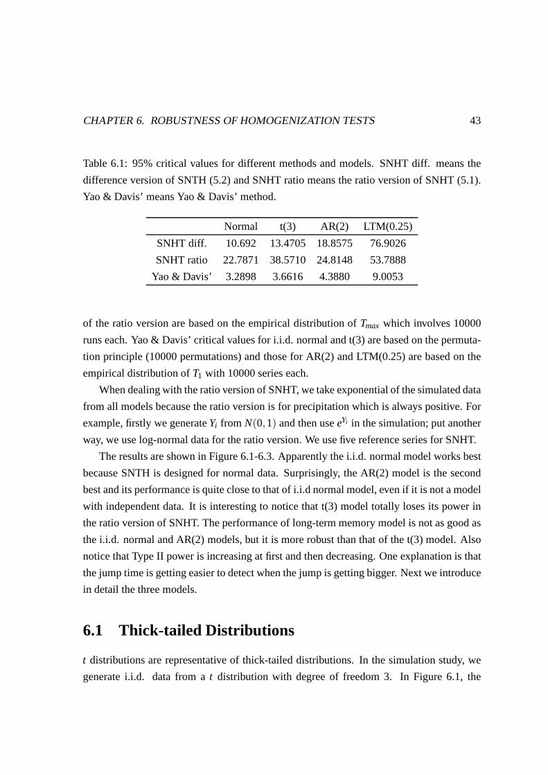
Table 6.1: 95% critical values for different methods and models. SNHT diff. means the

difference version of SNTH (5.2) and SNHT ratio means the ratio version of SNHT (5.1).

Yao & Davis’ means Yao & Davis’ method.

Normal t(3) AR(2) LTM(0.25)

SNHT diff. 10.692 13.4705 18.8575 76.9026

SNHT ratio 22.7871 38.5710 24.8148 53.7888

Yao & Davis’ 3.2898 3.6616 4.3880 9.0053

of the ratio version are based on the empirical distributionof Tmax which involves 10000

runs each. Yao & Davis’ critical values for i.i.d. normal andt(3) are based on the permuta-

tion principle (10000 permutations) and those for AR(2) andLTM(0.25) are based on the

empirical distribution ofT1 with 10000 series each.

When dealing with the ratio version of SNHT, we take exponential of the simulated data

from all models because the ratio version is for precipitation which is always positive. For

example, firstly we generateYi from N(0,1) and then useeYi in the simulation; put another

way, we use log-normal data for the ratio version. We use five reference series for SNHT.

The results are shown in Figure 6.1-6.3. Apparently the i.i.d. normal model works best

because SNTH is designed for normal data. Surprisingly, theAR(2) model is the second

best and its performance is quite close to that of i.i.d normal model, even if it is not a model

with independent data. It is interesting to notice that t(3)model totally loses its power in

the ratio version of SNHT. The performance of long-term memory model is not as good as

the i.i.d. normal and AR(2) models, but it is more robust thanthat of the t(3) model. Also

notice that Type II power is increasing at first and then decreasing. One explanation is that

the jump time is getting easier to detect when the jump is getting bigger. Next we introduce

in detail the three models.

6.1 Thick-tailed Distributions

t distributions are representative of thick-tailed distributions. In the simulation study, we

generate i.i.d. data from at distribution with degree of freedom 3. In Figure 6.1, the


0 0.5 1 1.5 2 2.5 30

0.5

1

Typ

e I P

ower

0 0.5 1 1.5 2 2.5 30

0.5

1

Typ

e II

Pow

er

0 0.5 1 1.5 2 2.5 30

0.5

1

Typ

e I+

Typ

e II

i.i.d. Normali.i.d. t(3)AR(2)LTM(0.25)

Figure 6.1: Power curves of the difference version of SNHT


0 0.5 1 1.5 2 2.5 30

0.2

0.4

0.6

0.8

Typ

e I P

ower

0 0.5 1 1.5 2 2.5 30

0.5

1

Typ

e II

Pow

er

0 0.5 1 1.5 2 2.5 30

0.5

1

Typ

e I+

Typ

e II


Figure 6.2: Power curves of the ratio version of SNHT


0 0.5 1 1.5 2 2.5 30

0.5

1

Typ

e I P

ower

0 0.5 1 1.5 2 2.5 30

0.5

1

Typ

e II

Pow

er

0 0.5 1 1.5 2 2.5 30

0.5

1

Typ

e I+

Typ

e II


Figure 6.3: Power curves of Yao & Davis’ method


0 200 400 600 800 1000−10

0

10

20

30

t(3) sequence with a jump=10

0 200 400 600 800 10000

0.5

1

1.5

2x 10

11

exp(t(3))

Figure 6.4: The first panel shows an i.i.d.t(3) sequence with a jump=10 att = 500 and the

second panel shows the exponential of the sequence.


performance oft(3) is better than Long-term memory model but worse thanAR(2). Figure

6.3 shows a similar result as that of Figure 6.1. However, In Figure 6.2, it does not work

at all. There is no power fort(3) no matter how large the jump is. The explanation for

this phenomena is that whilet(3) is thick-tailed in terms of its PDF the exponential oft(3)

is even more thick-tailed (you can imagine that the PDF is getting close to a ’uniform’

distribution). Even if we take exponential before we add thejump, it will not be detected

unless the jump is extremely large. Figure 6.4 shows this idea. So we do not recommend

to use the ratio version of SNHT fort-distributed, or more generally, thick-tailed data.

6.2 Autoregressive Memory

The second model is AR(2):

xt = 0.2xt−1+0.1xt−2+ωt , t ≥ 3 (6.1)

x1 = 0,x2 = 0,ωt ∼ i.i.d.N(0,1) (6.2)

Its performance is slightly worse than i.i.d. normal model but much better than the other

two among all three methods.

6.3 Long-term Memory

The long-term memory model (LTM) is of the form (Shumway and Stoffer 2006)

(1−B)dxt =∞

∑j=0

π jBjxt = ωt , 0< d < 0.5 (6.3)

whereB is the backshift operator (e.g.Bxt = xt−1, B2xt = xt−2), xt is the time series,ωt is

the white noise with varianceσ2, Γ is the gamma function and

π j =Γ( j −d)

Γ( j +1)Γ(−d)(6.4)

By algebraic calculation (Shumway and Stoffer 2006),

xt =∞

∑j=0

ψ jωt− j ,ψ j =Γ( j +d)

Γ( j +1)Γ(d)(6.5)


0 100 200 300 400 500 600 700 800 900 1000−4

−2

0

2

4

Long−term memory series

0 100 200 300 400 500 600 700 800 900 1000−0.1

0

0.1

0.2

0.3

Autocorrelation function

Figure 6.5: One simulated long-term memory series and its autocorrelation function with

d = 0.25.


Figure 6.5 shows one simulated long-term memory series and its autocorrelation func-

tion. In the simulation study,d = 0.25. Its performance is not so good as those of i.i.d.

normal and AR(2) models but it does reasonably well, especially when the jump is large

enough. This model is of great importance in climate study because most climate data are

long-term memory.

Chapter 7

Application to Barkerville, BC

7.1 Background of the Data

We have daily temperature and precipitation data of Barkerville, BC from Feb, 1888 to

Jan, 2007. In this thesis we use monthly mean temperature andmonthly total precipitation.

There are 1430 months but some observations are missing. We also have four incomplete

reference series from Dome Creek, Horsefly Lake Gruhs Lake, Mcbride 4SE and Quesnel

which are all less than 100 kilometers away from Barkerville. The monthly data are shown

in Figure 7.1 and 7.2. We apply SNHT and Yao & Davis’ method to the climate data. Note

that there is a sudden increase in the middle of the monthly total precipitation series of

Barkerville. That is because the number of rainy days are more than those of other periods.

Because the series are incomplete, we use the data from Dome Creek to fill up the gap

in the Barkerville data, and combine the data from Horsefly Lake Gruhs Lake, Mcbride

4SE and Quesnel to create a new reference series. However, there still exist some missing

values. There are 71 and 216 missing values in the new Barkerville and new reference

series for temperature and 60 and 196 for precipitation, respectively.

Next step is to find out if using different replacement valuesfor the missing data will

give significantly different results. We create 10000 random permutations of the raw data

(the missing values are not included) and replace the missing data with the firstn values of

each permutation, wheren is the number of missing values for each sequence. Thus there

are 10000 values of jump time andTmax for each test. Figure 7.3-7.5 show the result. It

seems that the replacement values do have significant effecton both the jump time and the

51

CHAPTER 7. APPLICATION TO BARKERVILLE, BC 52

200 400 600 800 1000 1200 1400−20−10

010

BA

RK

ER

VIL

LE

200 400 600 800 1000 1200 1400

−20−10

010

DO

ME

200 400 600 800 1000 1200 1400

−100

10

HO

RS

EF

LY

200 400 600 800 1000 1200 1400

−20−10

010

MC

BR

IDE

200 400 600 800 1000 1200 1400

−20

0

20

QU

ES

NE

L

Monthly Mean Temperature

Figure 7.1: Temperature series of Barkerville


200 400 600 800 1000 1200 14000

200

400

BA

RK

ER

VIL

LE

200 400 600 800 1000 1200 1400

50100150200

DO

ME

200 400 600 800 1000 1200 1400

100

200

HO

RS

EF

LY

200 400 600 800 1000 1200 1400

50100150200

MC

BR

IDE

200 400 600 800 1000 1200 1400

50

100

150

QU

ES

NE

L

Monthly Total Precipitation

Figure 7.2: Precipitation series of Barkerville


0 200 400 600 800 1000 1200 14000

500

1000

1500

jum

p tim

e

0 10 20 30 40 50 60 700

5

10

15

20

Tm

ax

Figure 7.3: Histograms of detected jumps and jump times using different replacement val-

ues with SNHT for temperature


200 400 600 800 1000 1200 14000

2000

4000

6000

8000

jum

p tim

e

1 1.5 2 2.50

10

20

30

40

50

Tm

ax


ues with Yao & Davis’ method for temperature


200 400 600 800 1000 1200 14000

2000

4000

6000

jum

p tim

e

0 200 400 600 800 1000 1200 14000

200

400

600

Tm

ax


ues with SNHT for precipitation


0 200 400 600 800 1000 1200 1400−0.1

−0.05

0

0.05

0.1

Lag

Tem

pera

ture

0 200 400 600 800 1000 1200 1400−0.1

−0.05

0

0.05

0.1

Lag

Pre

cipi

tatio

n

Figure 7.6: ACF of the modified Barkerville series

maximum value ofT, which means we must take this into account when interpreting the

final result. Note that there is no Yao & Davis’ method for precipitation since this method

requires i.i.d. data with the mean of the error being 0.

In the final analysis, we use seasonal average to replace the missing data. That is, we

use the average of all January observations to replace the missing January values, and use

the average of all February observations to replace the missing February values, etc.

To figure out which model (or more specifically, which critical value) we should use, we

subtract the corresponding seasonal average from every observation to remove the seasonal

trend for temperature (we cannot do this to precipitation because it is always positive).

The sample autocorrelation functions of the adjusted data are in Figure 7.6 (Generated in

R), which seems from a long-term memory model. Table 7.1 shows the estimates of the

parameterd in the long-term memory model. The 95% confidence intervals of d for both

temperature and precipitation do not include 0, which meansthe critical values for long-

term memory model apply (based on 10000 series and not shown in Table 6.1). The values


Table 7.1: Estimate of the LTM parameterd and its 95% CI

MLE Lower bound Upper bound

Temperature 0.127 0.067 0.188

Precipitation 0.066 0.010 0.124

in the table are computed by a package in R provided by Dr. Peter Guttorp.

7.2 Conclusion

The results are shown in Figure 7.7 and 7.8. There is no significant jump in the temperature

data but three possible jumps in the precipitation data.

We have scanned copies of the inspection binder after 1953 obtained from Monitoring

Operations Center in Richmond, BC. However, the inspectionbinder before 1953 was lost

in a fire. In the inspection binder of May 1975, it writes:

’The initial installation was in the road for snow removal, sothe observer moved it 200’

to the north. This didn’t affect the instrument exposure.’

As a result, there is a relocation of equipment in May, 1975 (corresponding to t = 1049)

which may still be the reason for the last jump of precipitation if we take the replacement

values into account (Figure 7.7).


200 400 600 800 1000 1200 1400

10

20

30

T s

erie

s of

tem

pera

ture

One of the max is obtained at t = 1052

200 400 600 800 1000 1200 1400

10

20

30

40

T s

erie

s of

pre

cipi

tatio

n

Max is obtained at t = 507, t = 726 and t = 996; That is, 3rd 1930, 6th 1948 and 12th 1970

Figure 7.7: The result of SNHT: dash lines denote the 95% critical values. Replace missing

values with seasonal average. Use 95% critical value of LTM(0.127) for temperature and

95% critical value of LTM(0.066) for precipitation. There is a relocation in May, 1975(t =

1049) which may cause the last jump of the precipitation.

200 400 600 800 1000 1200 1400

0.5

1

1.5

2

T1

serie

s of

tem

pera

ture

Max is obtained at t = 226 and t = 1048

Figure 7.8: Yao & Davis’ method: the 95% critical value of LTM(0.127) is far above the

dots (about 5.7).

Chapter 8

Discussion

8.1 Lowess

It is also interesting to apply some smooth techniques to thesimulated data. Figure 8.1

shows an example of locally weighted scatter plot smoothing(Lowess) with standard i.i.d.

normal data. We tried five different jump values and it seems that the smoothed curves try

to hide the jumps.

8.2 Multiple Jumps

In the simulation study we only deal with one jump. We can alsotry multiple jumps as well.

For simplicity, we only tried two jumps. The number of observations in each series is 1000

and we add two same jump values att = 333 andt = 667, where jump = 0.1,0.2,. . . ,3.0.

Figure 8.2 shows the plots of the distance between the estimated and the true jump times.

The estimates tend to come towards the middle of the series. One explanation of this

phenomena is that the performance at the boundary is unstable.

60

CHAPTER 8. DISCUSSION 61

0 200 400 600 800 1000

−2

0

2

jump = 0.1

0 200 400 600 800 1000−2

0

2

jump = 0.5

0 200 400 600 800 1000

−2024

jump = 1

0 200 400 600 800 1000−2

024

jump = 2

0 200 400 600 800 1000−2

0246

jump = 3

Figure 8.1: Lowess. The span = 10% of the sample size.

CHAPTER 8. DISCUSSION 62

−500 0 500−500

0

500

−500 0 500−500

0

500

−500 0 500−500

0

500

−500 0 500−200

0

200

−200 0 200−200

0

200

−200 0 200−200

0

200

−200 0 200−200

0

200

−200 0 200−200

0

200

−200 0 200−200

0

200

−200 0 200−200

0

200

−200 0 200−200

0

200

−200 0 200−200

0

200

−200 0 200−200

0

200

−200 0 200−200

0

200

−200 0 200−200

0

200

−200 0 200−200

0

200

−200 0 200−200

0

200

−200 0 200−200

0

200

−200 0 200−200

0

200

−200 0 200−200

0

200

−200 0 200−50

0

50

−100 0 100−200

0

200

−200 0 200−200

0

200

−200 0 200−50

0

50

−200 0 200−200

0

200

−100 0 100−100

0

100

−100 0 100−100

0

100

−50 0 50−50

0

50

−20 0 20−100

0

100

−50 0 50−50

0

50

Figure 8.2: Scatterplot of the differences between the estimated and the true jump times

(which can be positive or negtive). X-axis is for the first jump and Y-axis for the second

jump. The first five graphs at the first row are for jump = 0.1, 0.2, 0.3, 0.4, 0.5, etc. Each

graph involves 1000 points.

Chapter 9

Literature Review of DOL Problem

9.1 Load-Duration Effects in Western Hemlock Lumber

This review is based onLoad-Duration Effects in Western Hemlock Lumberby Foschi and

Barrett (1982).

The duration-of-load adjustment is important to the strength of wood to obtain design

stress. An experiment on load-duration effects in bending for western hemlock lumber had

been underway since 1977 at Forintek Canada Corporation’s Western Lab. The material

tested was western hemlock lumber.

A control group (N=150) was tested to failure with a ramp loading of short duration

to establish the basic short-term strength distribution. Two stress levels were chosen for

long-term tests corresponding to the 20th-percentile and the 5th-percentile of the short-

term strength distribution. Five groups of N=100 specimenseach were assigned to the two

long-term tests. The times to failure were ranked and the corresponding CDF computed in

the paper.

The experiment only involved two constant levels. In reality, however, most loads

produce stress of a random, cyclic nature superimposed on a constant stress produced by

permanent loads. Thus it is important to be able to extrapolate constant load test results to

predict the behavior for practical load situations.

The Damage Accumulation Model is proposed:

dαdt

= aeω1RN

(τ(t)− τo

τs

)b

+λeω2VNα (9.1)

63

CHAPTER 9. LITERATURE REVIEW OF DOL PROBLEM 64

where

• α(t) is a measure of damage which is defined such thatα = 0 corresponds to undamaged

material andα = 1 corresponds to failure.

• a,b,λ,ω1 andω2 are parameters.

• RN andVN are standard random normal variables.

• τ(t) is the stress applied to the member.

• τo is a threshold that must be exceeded for damage to accumulate.

• τs is the stress at which the specimen will break in a short-termtest.

• σ = τ(t)/τs is called the applied stress ratio.

• σo = τo/τs is called the threshold stress ratio. It is assumed that stress thresholdτo varies

between members in direct proportion to the short term stress τs, so the threshold stress

ratio σo is a constant. Usuallyσo < σ < 1.

Two tests are considered:

Short-Term Test

This is a ramp-load test of short duration where the load increases linearly with time at

a rateks to failure in timeTs and the strengthτs is reached:

τ(t) = kst, τs= τ(Ts) = ksTs, α(Ts) = 1 (9.2)

There is no closed form of the solution to (9.1) with the abovesettings. We can resort

to numerical solutions using Matlab, for instance.

Constant Load Test

The load is increased linearly with time at the rateks until the stress levelτc is reached

in a timeTL. This level is then held constant until failure occurs at timeTc.

τc = τ(TL) = ksTL (9.3)

In this case, (9.1) must be integrated in two steps: damage accumulation during the loading

phase and during the constant phase. Again, we can resort to numerical solutions.

We use different combinations of parameter values to conduct simulation and obtain

the predicted CDFs for time to failure for each of the two tests and minimize the deviation:

ψ =

{ N

∑i=1

[log(T)∗i − log(T)i

]2}1/2

(9.4)


whereN is the total number of tests (including short-term and constant load tests) and

log(T)i is the simulated value corresponding to the same probability level as the test result

log(T)∗i in the experiment.

The Damage Accumulation Model has been verified and showed anagreement with

the experimental results. It brings together the strength of wood members and the loads to

which they are subjected, allowing an assessment of the reliability of wood structures in a

systematic manner.

However, the experiment only covered one species in bending. It is important to explore

the effect of these constraints, considering other speciesand sizes in further research.

9.2 Probabilistic Modeling of Duration of Load Effects in

Timber Structures

This review is based onProbabilistic Modeling of Duration of Load Effects in Timber

Structuresby Kohler and Svensson (2002).

Initial load-carrying capacity of structural timber is determined by loading an undam-

aged structural timber with a ramp load with constant loading rate until failure. This ca-

pacity is frequently referred to as the short-term capacityor short-term strength.

Two models we are interested in are (there is a third model butwith limited knowledge

of wood engineering, I will skip it):

Gerhards’ model:dαdt

= e−a+bS(t)

R0 (9.5)

where

• α(t) is the degree of damage such thatα = 0 corresponds to undamaged material and

α = 1 corresponds to failure.

• R0 is the short-term capacity.

• S(t) is the load.

• a,b are parameters.

Gerhards’ model can be solved under constant or ramp load stress situation.


Foschi and Yao’s Model:

dαdt

= A

(S(t)R0

−η)B

+C

(S(t)R0

−η)D

α(t), S(t)> ηR0 (9.6)

where

• α(t) is the degree of damage such thatα = 0 corresponds to undamaged material and

α = 1 corresponds to failure

• R0 is the initial capacity

• S(t) is the load

• A,B,C,D are parameters

• η is the threshold ratio, which is between 0 and 1, the latter bound referring to material

not affected by DOL.

This model can be solved under constant or ramp load stress situation.

The parameter assessment may be performed by introducing anerror termε:

t f = t f ,m(SR,θ)+ ε (9.7)

where

• t f ,m(SR,θ) is the general form of the time to failure of the above three models as a function

of the ratio between applied load to short-term strengthSR (0 < SR < 1) and a vector of

model parametersθ.

• ε is assumed to be normal with mean 0 and unknown standard deviation σε.

Maximum Likelihood method is used to estimate the mean values and covariance ma-

trix for θ andσε. The parameters of the models are calibrated on results fromlong-term

tests (Hoffmeyer, 1990).

The damage accumulation for the case of constant load for thedamage models is sig-

nificantly different. Gerhard’s model shows linearity of damage accumulation with time

while the others show highly non-linear behavior.

9.3 Duration of Load Effects And Reliability Based De-

sign

This review is based onDuration of Load Effects and Reliability Based Designby Foschi

and Yao (1986).


The introduction of reliability-based design in wood structures requires consideration

of the effects that load duration has on degradation of strength over time. The reliability

estimation is complicated by the fact that load history mustbe taken into account, not only

load magnitudes. Central to the solution of this problem is the availability of a DOL model

which allows the estimation of the degradation effect for any load sequence.

This paper considers the superposition of dead and live loads (such as snow). The in-

formation normally available for snow loads is the distribution of annual maximum, which

can be represented by an Extreme Type I distribution (a.k.a.Gumbel):

S=U +[−ln(−ln p)]/C (9.8)

or

Fmax(S) = exp

(−exp(−C(S−U))

)(9.9)

where

• p is a random number uniformly distributed between 0 and 1.

• U andC are distribution parameters.

• Fmax(S) is the CDF ofS.

Note: The valuep0 corresponding toS= 0 in (9.8) is the probability of no snow.

A snow design loadSn is chosen for a 30-year period withp= 29/30. The ratio ofS/Sn

of annual maximum to design load is also Gumbel-distributedaccording to

S/Sn =U∗+[−ln(−ln p)]/C∗ (9.10)

where

U∗ =CU

CU+3.3843,C∗ =CU+3.3843 (9.11)

In general, the duration of the maximum annual load is not known, but the duration of the

winter may be assumed to be 5 months (Nov.1 - Apr.1). Assume the annual load comes

in NS segments of equal duration and that within each segmentthe load remains constant.

The segment loads are assumed to be independent of each otherand equally distributed.

For consistency, this distribution must be such that the distribution for the maximum of the

NS segment loads equals that for the annual maximum load.


If F(S) is the segment load distribution andpe is the probability of snow in a segment,

Fmax(S) = [(1− pe)+ peF(S)]NS (9.12)

wherepe must satisfy

(1− pe)NS= p0 (9.13)

Introducing (9.9) into (9.12), the distribution ofS is

S=U +(−ln(−NS ln[(1− pe)+ pe p]))/C (9.14)

and the distribution of the ratiox of the segment loadS to the designSn becomes

S/Sn = x=CU+(−ln(−NS ln[(1− pe)+ pe p]))

CU+3.3843(9.15)

The dead loadD may be assumed normally distributed with CV =CD (CV = coefficient

of variation, which is defined as standard deviation over mean). If the design dead loadDn

is taken equal to the mean value, the ratiod of the dead load to the design dead load is

D/Dn = d = 1+CDpn (9.16)

wherepn is a standard normal variable.

A load sequence for NY years, with NS load segments per winterwill contain (NY×NS+1) independent random variables:NY×NSlive loads and a dead load.

The load at any segment will be

D+S= Sn(dγ+x) (9.17)

where

γ = Dn/Sn, d = D/Dn ∼ Normal, x= S/Sn ∼ Gumbel (9.18)

The design equation used in the Canadian code CAN3-086.1-84has the following form:

1.25Dn+1.50Sn = φR(0.05) (9.19)

where

• φ is the performance factor applied to the characteristic strengthR(0.05). R(0.05) is the

5th-percentile of the short-term strength distribution.


Rewrite (9.19):

Sn = φR(0.05)/(1.25γ+1.50) (9.20)

when introduced in (9.17),

D+S=φR(0.05)

1.25γ+1.50(dγ+x) (9.21)

Note:x= 0 during summer.

The main objective is to derive (9.21) so that we can generatedata from it and use the

data to test different models, such as Foschi and Yao’s model(9.6) in the previous review.

Chapter 10

Markov Chain Monte Carlo

Markov Chain Monte Carlo (MCMC) is a general method based on drawing values of pa-

rameterθ from approximate distributions and then correcting those draws to better approx-

imate the target posterior distribution,p(θ|y), wherey is the data obtained. The samples

are drawn sequentially, with the distribution of the sampled draws depending on the last

value drawn.

The key to MCMC is to create a Markov process whose stationarydistribution is the

specifiedp(θ|y) and run the simulation long enough so that the distribution of the current

draws is close enough to this stationary distribution (Gelman et al. 2003).

The Metropolis-Hastings algorithm is a general term for a family of MCMC methods

that are useful for drawing samples from posterior distributions. Metropolis-Hastings al-

gorithm is a generalization to the Metropolis algorithm.

The Metropolis-Hastings algorithm is an adaptation of a random walk that uses an

acceptance/rejection rule to converge to the specified target distribution. It proceeds as

follows (Gelman et al. 2003):

• Draw a starting pointθ0, for which p(θ0|y)> 0, from a starting distributionp0(θ).• For t=1,2,. . . , sample a proposalθ∗ from a proposal distribution at timet: Jt(θ∗|θt−1),

which can depend on the iteration numbert. The Metropolis algorithm requires the pro-

posal distribution to be symmetric, satisfying for anyθa,θb andt:

Jt(θa|θb) = Jt(θb|θa)

while the Metropolis-Hastings algorithm does not have suchrequirement.

70

CHAPTER 10. MARKOV CHAIN MONTE CARLO 71

• For Metropolis-Hastings algorithm, calculate the ratio ofthe densities, which is cor-

rected for the asymmetric proposal rule,

r =p(θ∗|y)/Jt(θ∗|θt−1)

p(θt−1|y)/Jt(θt−1|θ∗)

For the Metropolis algorithm, since the proposal distribution is symmetric,

r =p(θ∗|y)

p(θt−1|y)

• Set

θt =

θ∗ with probability min(r,1)

θt−1 otherwise

It can be proved that the sequence of iterationsθ1,θ2, . . . converges to the target distri-

bution. MCMC also applies to multiple-parameter cases.

The Metropolis-Hastings algorithm can be viewed as a stochastic version of a stepwise

mode-finding algorithm, always accepting steps that increase the density but only some-

times accepting downward steps because for example, ifp(θ∗|y)> p(θt−1|y) in Metropolis

algorithm, thenr > 1, which meansθt = θ∗ for sure (Gelman et al. 2003).

Chapter 11

Simulation

11.1 Models

It is of great importance in the determination of safe and efficient engineering design prop-

erties for all wood products. Three models are widely used inthe duration of load problem.

They are Madison curve, Exponential Damage Rate model (EDRM) and Barrett and Foschi

I model (B/F I) (Cai et al. 2000).

The Madison Curve is:

dαdt

= A(τ− τ0)B, A> 0,B> 0 (11.1)

where

• α(t) is a measure of damage which is defined such thatα = 0 corresponds to undamaged

material andα = 1 corresponds to failure.

• A,B are parameters.

• τ = τ(t) is the stress applied to the lumber.

• τ0 is a constant that must be exceeded for damage to accumulate for the lumber.

We only consider a ramp load test where the applied stress is increased linearly over

time until the lumber breaks

τ(t) = kt (11.2)

Thus, the break time of the Madison curve under linear stressis:

T =1k

{[k(B+1)

A

] 1B+1

+ τ0

}(11.3)

72

CHAPTER 11. SIMULATION 73

The Exponential Damage Rate model (EDRM) is:

dαdt

= exp(−A+Bτ), A> 0,B> 0 (11.4)

where

• α(t) is the measure of damage.

• A,B are parameters.

• τ = τ(t) is the stress applied to the lumber.

The break time of EDRM under ramp load test is:

T =1

Bklog(1+BkeA) (11.5)

The Barrett and Foschi I model (BFI) is:

dαdt

= A(τ− τ0)BαC, A> 0,B> 0,0<C< 1 (11.6)

The break time of B/F I model under ramp load test is:

T =1k

{[k(B+1)A(1−C)

] 1B+1

+ τ0

}(11.7)

However,A andC in the B/F I model are not identifiable. If we setA(1−C) to be a single

parameter, then this model is equivalent to the Madison curve. Hence, we focus on the first

two models.

11.2 MCMC

Specifically, we deal with

log(Ti j ) = log

(1k j

{[k j(Bi j +1)

Ai j

] 1Bi j +1

+ τ0

})+ei j (11.8)

and

log(Ti j ) = log

(1

Bi j k jlog(1+Bi j k je

Ai j )

)+ei j (11.9)

wherei = 1, . . . , I , j = 1, . . . ,J. We letei j ∼N(0,10−6) because in practice the break time is

recorded by a computer so the measurement error can be ignored and we are not interested

in it.


We apply the hierarchical model:

log(Ai j )∼ N(µA,σ2A), log(Bi j )∼ N(µB,σ2

B) (11.10)

We tale log ofA,B and the break time because they are all positive. We set the prior

distributions of the hyper-parameters as below:

µA ∼ N(0,106),µB ∼ N(0,106) (11.11)

σA ∼Uni f (0,100),σB ∼Uni f (0,100) (11.12)

Our simulation works as follows. Firstly, we use the following settings to generate two

data sets from Madison model:

log(A) = 1.0, log(B) =−1.0 (11.13)

whereA andB are the two parameters in Madison model. Note thatτ0 is always set to 0.2

in the Madison model. The two data sets are corresponding to two scenarios:

Scenario I: we usek= [0.1,0.3, . . .,0.9] (thusJ = 5) and generateI = 20 observations

Ti j for eachk. Then we use this data set for both models.

Scenario II: we usek= [0.1,0.2, . . .,1.0] (thusJ= 10) and generateI = 10 observations

Ti j for eachk. Then we use this data set for both models.

Note that the number of observations is always 100. Secondly, we use the following

settings to generate two data sets from EDRM:

log(A) = 1.0, log(B) =−1.0 (11.14)

whereA andB are now the two parameters in EDRM. The two data sets are corresponding

to the same scenarios above. We useWinbugsto run the simulation which are based on

10000 iterations each. The code is attached as Appendix C.

Once we obtain the posterior distributions ofµA,µB,σA,σB, we can use their means as

estimates and then figure out the distributions ofA andB. Since we are actually interested

in the distribution of the break time, we generate 1000 values ofA andB, and thus compute

1000 values of the break time so we can compute the kernel smoothing density estimate,

which are shown in Figure 11.1 and 11.2.


0 2 4 6 80

0.5

1

1.5

2

2.5

3

3.5

4

Den

sity

(5k

s)

k=0.1

1 1.5 2 2.5 3 3.5 40

0.5

1

1.5

2

2.5

3

3.5

4

Den

sity

(10

ks)

0.5 1 1.5 2 2.50

0.5

1

1.5

2

2.5

3

3.5

4 k=0.5

0.5 1 1.5 2 2.50

1

2

3

4

5

Breaktime (in Hours) (data simulated from Madison function)

0 0.5 1 1.5 20

1

2

3

4

5 k=0.9

0 0.5 1 1.5 20

1

2

3

4

5

MadisonEDRM

Figure 11.1: PDFs of break time for different models, different values ofk and different

scenarios when the data is generated from Madison model.

0 10 20 30 400

0.05

0.1

0.15

0.2

0.25

Den

sity

(5k

s)

k=0.1

0 10 20 30 400

0.05

0.1

0.15

0.2

0.25

0.3

0.35

0.4

Den

sity

(10

ks)

0 5 10 15 20 25 300

0.05

0.1

0.15

0.2

0.25

0.3

0.35 k=0.5

0 5 10 15 200

0.05

0.1

0.15

0.2

0.25

0.3

0.35

0.4

Breaktime (in Hours) (data simulated from EDRM function)

0 5 10 15 20 25 300

0.1

0.2

0.3

0.4

0.5

0.6

0.7 k=0.9

0 5 10 15 200

0.1

0.2

0.3

0.4

0.5

0.6

0.7

MadisonEDRM

Figure 11.2: PDFs of break time for different models, different values ofk and different

scenarios when the data is generated from EDRM model.

Chapter 12

Conclusion and Discussion

12.1 Conclusion

We can also compute the means and the standard deviations fordifferent distributions in

Figure 11.1 and Figure 11.2, which is shown in Table 11.1 and 11.2.

From the table we can conclude that standard deviation decreases whenk increases.

We can also see that in general, if the data is generated from Madison model, the stan-

dard deviation for Madison model is smaller than the counterpart for EDRM; if the data

is generated from EDRM, the standard deviation for Madison model is greater than the

counterpart for EDRM, which is reasonable. Standard deviation of Scenario II is smaller

than the counterpart of Scenario I in each table, which meansreduction of noise does not

overcome the effect of have more values ofk. Moreover, whenk is larger, the difference

between Madison and EDRM is getting smaller in terms of mean.So we recommend to

use a largek when conducting experiments.

12.2 Discussion

If we fix the value ofk, there is no independent variable in

T =1k

{[k(B+1)

A

] 1B+1

+ τ0

}(12.1)

76


Table 12.1: Mean and standard deviation (SD) for each distribution when the data is gen-

erated from Madison model.

Scenario I k 0.1 0.5 0.9 k 0.1 0.5 0.9

Madisonmean

2.58 0.98 0.80SD

0.11 0.11 0.11

EDRM 1.77 1.21 0.96 0.41 0.21 0.16

Scenario II k 0.1 0.5 0.9 k 0.1 0.5 0.9

Madisonmean

2.61 1.00 0.83SD

0.10 0.10 0.10

EDRM 1.71 1.18 0.94 0.30 0.17 0.13

Table 12.2: Mean and standard deviation (SD) for each distribution when the data is gen-

erated from EDRM.

Scenario I k 0.1 0.5 0.9 k 0.1 0.5 0.9

Madisonmean

7.68 6.06 5.91SD

2.08 2.03 2.04

EDRM 12.39 7.26 5.41 3.05 1.24 0.80

Scenario II k 0.1 0.5 0.9 k 0.1 0.5 0.9

Madisonmean

7.90 6.29 6.11SD

1.34 1.33 1.32

EDRM 12.39 7.37 5.53 2.98 1.24 0.81


and we only have one break time for each lumber. This problem can lead to a more general

conclusion: if a model

y= f (A,B) (12.2)

has no independent variable, then it is impossible to estimate the parameters of Model

(12.2) by MCMC. We can not use the information ofy to recover the information ofA and

B. Put another way, we can think of (12.1) as

y= f (A,B)+x (12.3)

with data only available atx= 0. This model is actually a curve on the plane. It is impossi-

ble to determine a curve with two parameters using the data only at one value ofx because

the model involves two degrees of freedom.

The above conclusion holds for similar models with more thantwo parameters. How-

ever, if the model only involves one parameter, it can be estimated using data only available

at one value ofx because the degree of freedom of the model is also one.

As a result, we consider this model from another point of view: k can be the independent

variable because we can control the value ofk through a computer in practice. Then the

model reduces to a nonlinear model and we can either use leastsquares method or MCMC

to figure out the parameters and thus the break time.

Appendix A: Selection of Matlab code

for Chapter 3

We use Matlab as our main program to solve numerical problemsin Chapter 3. FDA

package used in Chapter 3 is posted on http://www.psych.mcgill.ca/misc/fda/.

Following is the matlab code for the FitzHugh-Nagumo equations; code for linear ODE

is quite similar:

odefn = @fhnfunode ;

fn . fn = @fhnfun ;

fn . d fdx = @fhndfdx ;

fn . d fdp = @fhndfdp ;

fn . d2fdx2 = @fhnd2fdx2 ;

fn . d2fdxdp = @fhnd2fdxdp ;

fn . d2fdp2 = @fhnd2fdp2 ;

fn . d3fdx3 = @fhnd3fdx3 ;

fn . d3fdx2dp = @fhnd3fdx2dp ;

fn . d3fdxdp2 = @fhnd3fdxdp2 ;

lambda = 1 e4 ;

y0 =[−1 ,1 ] ;

p a r s = [ 0 . 2 ; 0 . 2 ; 3 ] ;

sigma = 1 ;

t sp an = 0 : 0 . 1 : 2 0 ;

o b s_ p t s {1} = 1 :l e n g t h( t sp an ) ;

o b s_ p t s {2} = 1 :l e n g t h( t sp an ) ;

t f i n e = 0 : 0 . 0 5 : 2 0 ;

o d eo p t s = o d ese t ( ’ Re lTo l ’ ,1 e−8) ;

[ f u l l _ t i m e , f u l l _ p a t h ] = ode45( odefn , tspan , y0 , odeopts , p a r s ) ;

[ p l o t _ t i m e , p l o t _ p a t h ] = ode45( odefn , t f i n e , y0 , odeopts , p a r s ) ;

T c e l l = c e l l ( 1 ,s i z e( f u l l _ p a t h , 2 ) ) ;

p a t h _ c e l l = T c e l l ;

f o r j = 1 : l e n g t h( o b s_ p t s )

T c e l l { j } = f u l l _ t i m e ( o b s_ p t s { j } ) ;

p a t h _ c e l l { j } = f u l l _ p a t h ( o b s_ p t s { j } , j ) ;

end

wts = [ ] ;

lambda0 = 1 ;

n k n o t s = 201;

n o r d e r = 3 ;

79

APPENDIX A: SELECTION OF MATLAB CODE FOR CHAPTER 3 80

nquad = 5 ;

Y ce l l = p a t h _ c e l l ;

range = [min ( f u l l _ t i m e ) ,max( f u l l _ t i m e ) ] ;

k n o t s = l i n s p a c e( range ( 1 ) , range ( 2 ) , n k n o t s ) ;

n b a s i s = n k n o t s+norder−2;

q u ad v a l s = [ kno ts ’ ones (l e n g t h( k n o t s ) , 1 ) / n k n o t s ] ;

b a s i s _ c e l l = c e l l ( 1 ,l e n g t h( Y ce l l ) ) ;

L f d _ c e l l = c e l l ( 1 , l e n g t h( Y ce l l ) ) ;

b b a s i s = MakeBasis ( range , n b as i s , norder , kno ts , quadva ls, 1 ) ;

b a s i s _ c e l l ( : ) = { b b a s i s } ;

L f d _ c e l l ( : ) = { f d P a r ( b b as i s , 1 , lambda0 ) } ;

b b a s i s = MakeBasis ( range , n b as i s , norder , kno ts , quadva ls, 1 ) ;

A0= e v a l _ b a s i s ( kno ts , b b as i s , 0 ) ;

A1= e v a l _ b a s i s ( kno ts , b b as i s , 1 ) ;

h =1 / ( nkno ts−1) ;

W=ze r o s( nknots , n k n o t s ) ;

W( 1 ,1 ) =1 / 3∗h ;

W( nknots , n k n o t s )=1 /3∗h ;

f o r j =2 : ( nkno ts−1) ;

i f (mod ( j , 2 ) ==0 )

W( j , j )=4 /3∗h ;

e l s e W( j , j )=2 /3∗h ;

end

end

t o l _ v a l =1e−6;

o p t i o n s _ o u t = o p t i m s e t ( ’ D e r i v a t i v eCh eck ’ , ’ o f f ’ , . . .

’ Jaco b i an ’ , ’ o f f ’ , ’ D i sp l ay ’ , ’ o f f ’ , ’ Max I te r ’ , . . .

1000 , ’ TolFun ’ , t o l _ v a l , ’ TolX ’ , t o l _ v a l ) ;

o p t i o n s _ i n = o p t i m s e t ( ’ D e r i v a t i v eCh eck ’ , ’ o f f ’ , . . .

’ Jaco b i an ’ , ’ on ’ , ’ D i sp l ay ’ , ’ o f f ’ , ’ Max I te r ’ , . . .

1000 , ’ TolFun ’ , t o l _ v a l , ’ TolX ’ , t o l _ v a l , . . .

’ JacobMul t ’ , @SparseJMfun ) ;

backup =[0 .732∗sigma ,0 .9 8 2∗ sigma ,1 .3 4 5∗ sigma ] ;

t a b l e = c e l l ( 3 , 4 ) ;

sim =100;

s t a r t p a r s = p a r s ;

f o r mm=1 : 3 ;

f o r nn =1 : 4 ;

t h r e s h o l d =backup (mm) ;

p r o f i l e = ze r o s( sim , 3 ) ;

r o b u s t = ze r o s( sim , 3 ) ;

f o r i =1 : sim

Y ce l l = d a t a {nn }{ i } ;

DEfd = sm o o t h f d _ ce l l ( Yce l l , Tce l l , L f d _ c e l l ) ;

co e f s = g e t c e l l c o e f s ( DEfd ) ;

%p r o f i l i n g

f1=@( p a r ) Hnorm ( par , lambda , A0 , A1 , . . .

Yce l l ,W, coefs , o p t i o n s _ i n ) ;

b e t a1 = l s q n o n l i n ( f1 , s t a r t p a r s , [ ] , [ ] , o p t i o n s _ o u t ) ;

p r o f i l e ( i , : ) = beta1 ’ ;

%r o b u s t

f2=@( p a r ) H( par , lambda , A0 , A1 , Yce l l ,W, . . .

coefs , o p t i o n s_ i n , t h r e s h o l d ) ;

b e t a2 = l s q n o n l i n ( f2 , s t a r t p a r s , [ ] , [ ] , o p t i o n s _ o u t ) ;


r o b u s t ( i , : ) = beta2 ’ ;

d i s p l a y ( [ ’ S i m u l a t i o n = ’ , num2st r( [mm, nn , i ] ) ] ) ;

end

BIAS =[ mean( p r o f i l e ( : , 1 ) )− p a r s ( 1 ) , . . .

mean( r o b u s t ( : , 1 ) )− p a r s ( 1 ) ; . . .

mean( p r o f i l e ( : , 2 ) )− p a r s ( 2 ) , . . .

mean( r o b u s t ( : , 2 ) )− p a r s ( 2 ) ; . . .

mean( p r o f i l e ( : , 3 ) )− p a r s ( 3 ) , . . .

mean( r o b u s t ( : , 3 ) )− p a r s ( 3 ) ] ;

SE=[s t d( p r o f i l e ( : , 1 ) ) , s t d( r o b u s t ( : , 1 ) ) ; . . .

s t d( p r o f i l e ( : , 2 ) ) , s t d( r o b u s t ( : , 2 ) ) ; . . .

s t d( p r o f i l e ( : , 3 ) ) , s t d( r o b u s t ( : , 3 ) ) ] ;

RMSE=[s q r t ( ( p r o f i l e ( : ,1 )− p a r s ( 1 ) ) ’∗ . . .

( p r o f i l e ( : ,1 )− p a r s ( 1 ) ) / sim ) , . . .

s q r t ( ( r o b u s t ( : ,1 )− p a r s ( 1 ) ) ’ . . .

∗( r o b u s t ( : ,1 )− p a r s ( 1 ) ) / sim ) ; . . .

s q r t ( ( p r o f i l e ( : ,2 )− p a r s ( 2 ) ) ’ . . .

∗( p r o f i l e ( : ,2 )− p a r s ( 2 ) ) / sim ) , . . .

s q r t ( ( r o b u s t ( : ,2 )− p a r s ( 2 ) ) ’ . . .

∗( r o b u s t ( : ,2 )− p a r s ( 2 ) ) / sim ) ; . . .

s q r t ( ( p r o f i l e ( : ,3 )− p a r s ( 3 ) ) ’ . . .

∗( p r o f i l e ( : ,3 )− p a r s ( 3 ) ) / sim ) , . . .

s q r t ( ( r o b u s t ( : ,3 )− p a r s ( 3 ) ) ’∗ . . .

( r o b u s t ( : ,3 )− p a r s ( 3 ) ) / sim ) ] ;

t a b l e {mm, nn }=[ BIAS , SE ,RMSE] ;

end

end

Following is the matlab code for the Predator-Prey model:

d e l t a t r u = 0 . 6 8 ;

N i t r u = 8 0 ;

e p s i l o n t r u = 0 . 2 5 ;

l am b t r u = 0 . 4 ;

mtru = 0 . 0 5 5 ;

b c t r u = 3 . 3 ;

b b t r u = 2 . 2 5 ;

k c t r u = 4 . 3 ;

k b t r u = 1 5 . 0 ;

% t h e i n i t a l p a r am e t e r s

f i t s t r u c t . d e l t a = d e l t a t r u ;

f i t s t r u c t . Ni = N i t r u ;

f i t s t r u c t .m = mtru ;

f i t s t r u c t . e p s i l o n = e p s i l o n t r u ;

f i t s t r u c t . lamb = l am b t r u ;

f i t s t r u c t . bc = b c t r u ;

f i t s t r u c t . bb = b b t r u ;

f i t s t r u c t . kc = k c t r u ;

f i t s t r u c t . kb = k b t r u ;

d a t a = data068 ;

[ nobs , n co l ] = s i z e( d a t a ) ;

% c r e a t e b a s i s f o r a l l f o u r f u n c t i o n a l v a r i a b l e s


% d e l e t e t h e f i r s t t h r e e o b s e r v a t i o n s

sp = 3 ;

t o b s = d a t a ( sp : nobs , 1 ) ;

Cobs = d a t a ( sp : nobs , 2 ) ;

Bobs = d a t a ( sp : nobs , 3 ) ;

nobs = l e n g t h( t o b s ) ;

N i n i t = N i t r u ;

C i n i t = Cobs ( 1 ) ;

R i n i t = Bobs ( 1 ) ;

B i n i t = Bobs ( 1 ) ;

y i n i t = [ N i n i t , C i n i t , R i n i t , B i n i t ] ;

o d eo p t i o n s = o d ese t ( ’ Re lTo l ’ ,1 e−7, ’ AbsTol ’ ,1 e−7) ;

t f i n e = l i n s p a c e( t o b s ( 1 ) , t o b s ( nobs ) , 1 0 0 ) ;

% so l v e d i f f e r e n t i a l e q u a t i o n wi th ex ac t p a r am e t e r s

[ t o u t , so l u ] = ode45( @ppode , tobs , y i n i t , o d eo p t i o n s , f i t s t r u c t ) ;

[ t o u t , s o l u f i n e ] = ode45( @ppode , t f i n e , y i n i t , o d eo p t i o n s , . . .

f i t s t r u c t ) ;

Nsolu = so l u ( : , 1 ) ;

Cso lu = so l u ( : , 2 ) ;

Rso lu = so l u ( : , 3 ) ;

Bso lu = so l u ( : , 4 ) ;

conC = ( so l u ( : , 2 ) ’∗ Cobs ) / ( Cobs ’∗Cobs ) ;

conB = ( so l u ( : , 4 ) ’∗ Bobs ) / ( Bobs ’∗Bobs ) ;

d i s p l a y (num2st r( [ conC conB ] ) )

Cobs = Cobs .∗ conC ;

Bobs = Bobs .∗ conB ;

% i n i t i a l v a l u e f o r v a r i a b l e s

N i n i t = N i t r u ;

C i n i t = Cobs ( 1 ) ;

R i n i t = Bobs ( 1 ) ;

B i n i t = Bobs ( 1 ) ;

o d eo p t i o n s = o d ese t ( ’ Re lTo l ’ ,1 e−10, ’ AbsTol ’ ,1 e−10) ;

nos =6;

b e t a= c e l l ( nos , 1 ) ;

SSErob=ze r o s( nos , 1 ) ;

SSEpro=ze r o s( nos , 1 ) ;

SSEfus=ze r o s( nos , 1 ) ;

MSErob=ze r o s( nos , 1 ) ;

MSEpro=ze r o s( nos , 1 ) ;

MSEfus=ze r o s( nos , 1 ) ;

i n i t i a l = c e l l ( nos , 1 ) ;

f o r lam =1:6

y i n i t =g iven { lam } ;

% By my p r o f i l i n g code

p r o p a r . d e l t a = d e l t a t r u ;

p r o p a r . Ni = N i t r u ;

p r o p a r .m = e s t p r o { lam } ( 6 ) ;

p r o p a r . e p s i l o n = e s t p r o { lam } ( 5 ) ;

p r o p a r . lamb = e s t p r o { lam } ( 7 ) ;

p r o p a r . bc = e s t p r o { lam } ( 1 ) ;

p r o p a r . bb = e s t p r o { lam } ( 3 ) ;

p r o p a r . kc = e s t p r o { lam } ( 2 ) ;


p r o p a r . kb = e s t p r o { lam } ( 4 ) ;

% so l v e d i f f e r e n t i a l e q u a t i o n wi th ex ac t p a r am e t e r s

[ t o u t , so l u ] = ode45( @ppode , tobs , y i n i t , o d eo p t i o n s , p r o p a r ) ;

Nsolu = so l u ( : , 1 ) ;

Cso lu = so l u ( : , 2 ) ;

Rso lu = so l u ( : , 3 ) ;

Bso lu = so l u ( : , 4 ) ;

% c r e a t e b a s i s f o r N, C ,R and B

n o r d e r = 4 ;

k n o t s = l i n s p a c e( t o b s ( 1 ) , t o b s ( nobs ) , 1 0 0 ) ;

Tl im = max( t o b s ) ;

n b a s i s = l e n g t h( k n o t s ) + n o r d e r− 2 ;

b a s i s o b j = c r e a t e _ b s p l i n e _ b a s i s ( [ t o b s ( 1 ) , Tl im ] , [ ] , . . .

norder , k n o t s ) ;

% % s e t up q u a d r a t u r e p o i n t s and w e i g h t s

nquad = 3 ;

[ b a s i s o b j , quadpts , quadwts ] = q u ad se t ( nquad , b a s i s o b j ) ;

% smooth t h e d a t a wi th t h e s e v a l u es

lambdaN = 0 . 1 ;

NfdPar = f d P a r ( b a s i s o b j , 2 , lambdaN ) ;

[ NfdD2 , Ndf , Ngcv ] = sm o o t h _ b as i s ( tobs , Nsolu , NfdPar ) ;

lambdaC = 0 . 1 ;

CfdPar = f d P a r ( b a s i s o b j , 2 , lambdaC ) ;

[ CfdD2 , Cdf , Cgcv ] = sm o o t h _ b as i s ( tobs , Cobs , CfdPar ) ;

lambdaR = 0 . 1 ;

RfdPar = f d P a r ( b a s i s o b j , 2 , lambdaR ) ;

[ RfdD2 , Rdf , Rgcv ] = sm o o t h _ b as i s ( tobs , Rsolu , RfdPar ) ;

lambdaB = 0 . 1 ;

BfdPar = f d P a r ( b a s i s o b j , 2 , lambdaB ) ;

[ BfdD2 , Bdf , Bgcv ] = sm o o t h _ b as i s ( tobs , Bobs , BfdPar ) ;

% [ Ndf , Ngcv ; Cdf , Cgcv ; Rdf , Rgcv ; Bdf , Bgcv ] ;

% Resu l t by smooth d a t a wi th D2x ( t ) ,

% which a r e t h e i n i t i a l v a l u e o f co e f ;

Ncoef = g e t c o e f ( NfdD2 ) ;

Ccoef = g e t c o e f ( CfdD2 ) ;

Rcoef = g e t c o e f ( RfdD2 ) ;

Bcoef = g e t c o e f ( BfdD2 ) ;

coef0 = [ Ncoef ; Ccoef ; Rcoef ; Bcoef ] ;

% s e t up d a t a s t r u c t

% w e i g h t s f o r v a r i a b l e s

Nobs = Nsolu ;

Robs = Rso lu ;

Nwt = v a r ( Nobs ) ;

Cwt = v a r ( Cobs ) ;

Rwt = v a r ( Robs ) ;

Bwt = v a r ( Bobs ) ;

wt = [ Nwt , Cwt , Rwt , Bwt ] ;

% w e i g h t s f o r v a r i a b l e s


d a t s t r u c t . Nwt = Nwt ;

d a t s t r u c t . Cwt = Cwt ;

d a t s t r u c t . Rwt = Rwt ;

d a t s t r u c t . Bwt = Bwt ;

% d a t a

d a t s t r u c t . y = [ Cobs , Bobs ] ;

d a t s t r u c t . t o b s = t o b s ;

% b a s i s v a l u es a t sampl ing p o i n t s

b as i sm a t = e v a l _ b a s i s ( tobs , b a s i s o b j ) ;

Dbas ismat = e v a l _ b a s i s ( tobs , b a s i s o b j , 1 ) ;

d a t s t r u c t . b as i sm a t = b as i sm a t ;

d a t s t r u c t . Dbas ismat = Dbasismat ;

% b a s i s v a l u es a t q u a d r a t u r e p o i n t s

q u ad b as i sm a t = e v a l _ b a s i s ( quadpts , b a s i s o b j ) ;

s i z e( q u ad b as i sm a t ) ;

Dquadbas ismat = e v a l _ b a s i s ( quadpts , . . .

b a s i s o b j , 1 ) ;

d a t s t r u c t . q u ad p t s = q u ad p t s ;

d a t s t r u c t . quadwts = quadwts ;

d a t s t r u c t . q u ad b as i sm a t = q u ad b as i sm a t ;

d a t s t r u c t . Dquadbas ismat = Dquadbas ismat ;

% s e t up f i t s t r u c t t h a t c o n t a i n s needed i n f o f o r

% P P f i t and PPfn smooth d a t a wi th DIFEs

f i t s t r u c t . coef0 = coef0 ;

co e f = coef0 ;

t o l v a l = 1e−10;

i t e r m ax = 100;

t o l v a l = 1e−12;

o p t i o n sP P f n = o p t i m s e t ( ’ La r g eS ca l e ’ , ’ on ’ , . . .

’ D e r i v a t i v eCh eck ’ , ’ o f f ’ , ’ D i sp l ay ’ , . . .

’ i t e r ’ , ’ Max I te r ’ , i te rmax , . . .

’ TolCon ’ , t o l v a l , ’ TolFun ’ , t o l v a l , . . .

’ TolX ’ , t o l v a l , ’TolPCG ’ , t o l v a l , . . .

’ Jaco b i an ’ , ’ on ’ ) ;

gradwrd = 1 ;

lambda = ones ( 4 , 1 ) .∗ ( 0 . 1 ) ;

% i n i t i a l smooth ing

t i c

[ coef , resnorm , r e s i d u a l , e x i t f l a g ] = . . .

l s q n o n l i n ( @PPfitLS , coef0 , [ ] , [ ] , o p t i o n sP P f n , . . .

d a t s t r u c t , f i t s t r u c t , lambda , gradwrd ) ;

t o c

f i t s t r u c t . coef0 = co e f ;

[ nobs , n b a s i s ] = s i z e( d a t s t r u c t . b as i sm a t ) ;

ind1 = 1 : n b a s i s ;

ind2 = ( n b a s i s +1 ) : ( 2∗ n b a s i s ) ;

ind3 = (2∗ n b a s i s +1 ) : ( 3∗ n b a s i s ) ;

ind4 = (3∗ n b a s i s +1 ) : ( 4∗ n b a s i s ) ;

ph imat = d a t s t r u c t . b as i sm a t ;

% r e s u l t by smooth d a t a wi th DIFEs


Ncoef = co e f ( ind1 ) ;

Ccoef = co e f ( ind2 ) ;

Rcoef = co e f ( ind3 ) ;

Bcoef = co e f ( ind4 ) ;

t f i n e m a t = e v a l _ b a s i s ( t f i n e , b a s i s o b j ) ;

Nhat = t f i n e m a t∗Ncoef ;

Chat = t f i n e m a t∗Ccoef ;

Rhat = t f i n e m a t∗Rcoef ;

Bhat = t f i n e m a t∗Bcoef ;

% S e t up i n i t i a l v a l u es f o r t h e p a r am e t e r s ,

% h e r e we use t h e t r u e v a l u es .

p a r v e c t r u ( 1 ) = e p s i l o n t r u ;

p a r v e c t r u ( 2 ) = l am b t r u ;

p a r v e c t r u ( 3 ) = mtru ;

p a r v e c t r u ( 4 ) = b c t r u ;

p a r v e c t r u ( 5 ) = b b t r u ;

p a r v e c t r u ( 6 ) = k c t r u ;

p a r v e c t r u ( 7 ) = k b t r u ;

% e s t i m a t e a l l p a r am e t e r s ex cep t

% f i x e t h e f i r s t c o e f f i c i e n t t o be 0 ;

f i t s t r u c t . e s t i m a t e = ones ( 7 , 1 ) ;

e s t i n d = f i n d ( f i t s t r u c t . e s t i m a t e == 1 ) ;

% s e t t h e o p t i m i z a t i o n p a r am e t e r s f o r t h e o u t e r

% o p t i m i z a t i o n on ly f u n c t i o n v a l u es a r e used

% a t t h i s p o i n t

t o l v a l = 1e−10;

o p t i o n sP P f n = o p t i m s e t ( ’ La r g eS ca l e ’ , ’ on ’ , . . .

’ D e r i v a t i v eCh eck ’ , ’ o f f ’ , ’ D i sp l ay ’ , . . .

’ i t e r ’ , ’ Max I te r ’ , 50 , . . .

’ TolCon ’ , t o l v a l , ’ TolFun ’ , t o l v a l , . . .

’ TolX ’ , t o l v a l , ’TolPCG ’ , t o l v a l , . . .

’ Jaco b i an ’ , ’ on ’ ) ;

gradwrd = 1 ;

parvec0 = p a r v e c t r u ( e s t i n d ) ;

p a r v ec = parvec0 ;

lambda2 = ones ( 4 , 1 ) .∗ ( 1 0 ^ 2 ) ;

Y ce l l = c e l l ( 4 , 1 ) ;

Y ce l l {1}=Nobs ;

Y ce l l {2}=Cobs ;

Y ce l l {3}=Robs ;

Y ce l l {4}=Bobs ;

%Simpson ’ s r u l e

n k n o t s=l e n g t h( q u ad p t s ) ;

h =1 / ( nkno ts−1) ;

W=ze r o s( nknots , n k n o t s ) ;

W( 1 ,1 ) =1 / 3∗h ;

W( nknots , n k n o t s )=1 /3∗h ;

f o r j =2 : ( nkno ts−1) ;

i f ( mod ( j , 2 ) ==0 )

W( j , j )=4 /3∗h ;

e l s e W( j , j )=2 /3∗h ;

end

end


A0= q u ad b as i sm a t ;

A1=Dquadbas ismat ;

A2= b as i sm a t ;

co e f s =[ Ncoef ; Ccoef ; Rcoef ; Bcoef ] ;

t o l v a l = 1e−12;

o p t i o n s _ o u t = o p t i m s e t ( ’ D e r i v a t i v eCh eck ’ , ’ o f f ’ , . . .

’ Jaco b i an ’ , ’ o f f ’ , ’ D i sp l ay ’ , ’ i t e r ’ , ’ Max I te r ’ , . . .

100 , ’ TolFun ’ , t o l v a l , ’ TolX ’ , t o l v a l , . . .

’ MaxFunEval ’ , 1 0 0 0 0 ) ;

o p t i o n s _ i n = o p t i m s e t ( ’ D e r i v a t i v eCh eck ’ , ’ o f f ’ , . . .

’ Jaco b i an ’ , ’ o f f ’ , ’ D i sp l ay ’ , ’ i t e r ’ , ’ Max I te r ’ , . . .

100 , ’ TolFun ’ , t o l v a l , ’ TolX ’ , t o l v a l , . . .

’ JacobMul t ’ , @SparseJMfun , ’ MaxFunEval ’ , 1 0 0 0 0 ) ;

e p s i l o n p r o = 0 . 1 1 ;

lambpro = 0 . 0 1 ;

mpro = 0 . 1 5 2 ;

bcpro = 3 . 9 ;

bbpro = 1 . 9 7 ;

kcpro = 4 . 3 ;

kbpro = 1 5 . 7 ;

s t a r t p a r = l o g ( [ bcpro , kcpro , bbpro , kbpro , . . .

ep s i l o n p r o , mpro , lambpro ] ) ;

k1=s q r t ( 1 7 6 .0 7 4 3 / 1 1 )∗1 .3 4 5 ;

k2=s q r t ( 1 6 . 2 1 8 8 / 1 2 )∗1 . 3 4 5 ;

k =[ k1 , k2 ] ;

wt = 1 . / wt ;

t i c

lambda =10^( lam +1 ) ;

fun = @( p a r ) H( par , lambda , Yce l l ,W, A0 , A1 , A2 , . . .

coefs , o p t i o n s_ i n , k , wt ) ;

b e t a{ lam}= l s q n o n l i n ( fun , s t a r t p a r , [ ] , [ ] , o p t i o n s _ o u t ) ;

temp=@( c ) G( c ,b e t a{ lam } , lambda , Yce l l ,W, A0 , A1 , A2 , k , wt ) ;

C o e f i t = l s q n o n l i n ( temp , coefs , [ ] , [ ] , o p t i o n s _ i n ) ;

b e t a{ lam}= exp( b e t a{ lam } ) ;

t o c

mm=l e n g t h( C o e f i t ) ;

temp1=A0∗C o e f i t ( 1 : (mm/ 4 ) ) ;

temp2=A0∗C o e f i t ( (mm/ 4 +1 ) : ( 2∗mm/ 4 ) ) ;

temp3=A0∗C o e f i t ( (2∗mm/ 4 +1 ) : ( 3∗mm/ 4 ) ) ;

temp4=A0∗C o e f i t ( (3∗mm/ 4 + 1 ) :end) ;

i n i t i a l { lam }=[ temp1 ( 1 ) , temp2 ( 1 ) , temp3 ( 1 ) , temp4 ( 1 ) ] ;

r o b u s t . d e l t a = d e l t a t r u ;

r o b u s t . Ni = N i t r u ;

r o b u s t .m = b e t a{ lam } ( 6 ) ;

r o b u s t . e p s i l o n = b e t a{ lam } ( 5 ) ;

r o b u s t . lamb = b e t a{ lam } ( 7 ) ;

r o b u s t . bc = b e t a{ lam } ( 1 ) ;

r o b u s t . bb = b e t a{ lam } ( 3 ) ;


r o b u s t . kc = b e t a{ lam } ( 2 ) ;

r o b u s t . kb = b e t a{ lam } ( 4 ) ;

Fussmann . d e l t a = d e l t a t r u ;

Fussmann . Ni = N i t r u ;

Fussmann .m = 0 . 0 5 5 ;

Fussmann . e p s i l o n = 0 . 2 5 ;

Fussmann . lamb = 0 . 4 0 ;

Fussmann . bc = 3 . 3 ;

Fussmann . bb = 2 . 2 5 ;

Fussmann . kc = 4 . 3 ;

Fussmann . kb = 1 5 . 0 ;

[ junk , f u s ] = ode45( @ppode , tobs , y i n i t , . . .

o d eo p t i o n s , Fussmann ) ;

[ junk , f u s f i n e ] = ode45( @ppode , t f i n e , y i n i t , . . .

o d eo p t i o n s , Fussmann ) ;

C f u s f i n e = f u s f i n e ( : , 2 ) ;

B f u s f i n e = f u s f i n e ( : , 4 ) ;

Cfus = f u s ( : , 2 ) ;

Bfus = f u s ( : , 4 ) ;

[ junk , rob ] = ode45( @ppode , tobs , i n i t i a l { lam } , . . .

o d eo p t i o n s , r o b u s t ) ;

[ junk , r o b f i n e ] = ode45( @ppode , t f i n e , . . .

i n i t i a l { lam } , o d eo p t i o n s , r o b u s t ) ;

C r o b f i n e = r o b f i n e ( : , 2 ) ;

B r o b f i n e = r o b f i n e ( : , 4 ) ;

Crob = rob ( : , 2 ) ;

Brob = rob ( : , 4 ) ;

[ junk , p ro ] = ode45( @ppode , tobs , y i n i t , . . .

o d eo p t i o n s , p r o p a r ) ;

[ junk , p r o f i n e ] = ode45( @ppode , t f i n e , y i n i t , . . .

o d eo p t i o n s , p r o p a r ) ;

Cp r o f i n e = p r o f i n e ( : , 2 ) ;

Bp r o f i n e = p r o f i n e ( : , 4 ) ;

Cpro = pro ( : , 2 ) ;

Bpro = pro ( : , 4 ) ;

% compare Robust w i th P r o f i l i n g

h = f i g u r e ;

s u b p l o t( 2 , 1 , 1 )

p l o t ( tobs , Cobs , ’ ok ’ , ’ MarkerS ize ’ , 5 , ’ MarkerFace ’ , ’ k ’ )

ho ld on

p l o t ( t f i n e , C f u s f i n e , ’ : k ’ , ’ LineWidth ’ , 2 )

p l o t ( t f i n e , Cpro f ine , ’−−k ’ , ’ LineWidth ’ , 2 )

p l o t ( t f i n e , Crob f ine , ’−k ’ , ’ LineWidth ’ , 2 )

f o r i i =1 : l e n g t h( Cobs ) ;

i f abs( Cobs ( i i )−Crob ( i i ) ) > k1 ;

p l o t ( t o b s ( i i ) , Cobs ( i i ) , ’ ok ’ , ’ LineWidth ’ , . . .

2 , ’ MarkerS ize ’ , 1 2 )

end

end

ho ld o f f

x l im ( [ min ( t o b s ) ,max( t o b s ) ] ) ;

y l a b e l ( ’ C h l o r e l l a ’ , ’ F o n t S i ze ’ , 1 5 )

h legend =l eg en d( ’ Data ’ , ’ Fussmann ’ , . . .

’ P a r am e t e r Cascad ing ’ , ’ Robust ’ , ’ O u t l i e r ’ , 3 ) ;

s e t( h legend , ’ F o n t S i ze ’ , 8 ) ;

s u b p l o t( 2 , 1 , 2 )

p l o t ( tobs , Bobs , ’ ok ’ , ’ MarkerS ize ’ , 5 , ’ MarkerFace ’ , ’ k ’ )


ho ld on

p l o t ( t f i n e , B f u s f i n e , ’ : k ’ , ’ LineWidth ’ , 2 )

p l o t ( t f i n e , Bpro f ine , ’−−k ’ , ’ LineWidth ’ , 2 )

p l o t ( t f i n e , Brob f ine , ’−k ’ , ’ LineWidth ’ , 2 )

f o r i i =1 : l e n g t h( Bobs ) ;

i f abs( Bobs ( i i )−Brob ( i i ) ) > k2 ;

p l o t ( t o b s ( i i ) , Bobs ( i i ) , ’ ok ’ , ’ LineWidth ’ , . . .

2 , ’ MarkerS ize ’ , 1 2 )

end

end

ho ld o f f

x l im ( [ min ( t o b s ) ,max( t o b s ) ] ) ;

y l im ( [ 0 , 1 2 ] ) ;

x l a b e l ( ’ Time ( minu tes ) ’ , ’ F o n t S i ze ’ , 1 5 )

y l a b e l ( ’ B r ach i o n u s ’ , ’ F o n t S i ze ’ , 1 5 )

mm=0;

nn =0;

f o r i i =1 : l e n g t h( t o b s ) ;

i f abs( Cobs ( i i )−Crob ( i i ) ) > k1 ;

Crob ( i i )= Cobs ( i i ) ;

Cpro ( i i )= Cobs ( i i ) ;

Cfus ( i i )= Cobs ( i i ) ;

mm=mm+1;

end

i f abs( Bobs ( i i )−Brob ( i i ) ) > k2 ;

Brob ( i i )= Bobs ( i i ) ;

Bpro ( i i )= Bobs ( i i ) ;

Bfus ( i i )= Bobs ( i i ) ;

nn=nn +1;

end

end

SSErob ( lam ) = ( wt ( 2 )∗ ( Cobs−Crob ) ’∗ ( Cobs−Crob ) + . . .

wt ( 4 )∗ ( Bobs−Brob ) ’∗ ( Bobs−Brob ) ) ;

SSEpro ( lam ) = ( wt ( 2 )∗ ( Cobs−Cpro ) ’∗ ( Cobs−Cpro ) + . . .

wt ( 4 )∗ ( Bobs−Bpro ) ’∗ ( Bobs−Bpro ) ) ;

SSEfus ( lam ) = ( wt ( 2 )∗ ( Cobs−Cfus ) ’∗ ( Cobs−Cfus ) + . . .

wt ( 4 )∗ ( Bobs−Bfus ) ’∗ ( Bobs−Bfus ) ) ;

MSErob( lam )= SSErob ( lam ) / ( 2∗ l e n g t h( t o b s )−mm−nn ) ;

MSEpro( lam )= SSEpro ( lam ) / ( 2∗ l e n g t h( t o b s )−mm−nn ) ;

MSEfus ( lam )= SSEfus ( lam ) / ( 2∗ l e n g t h( t o b s )−mm−nn ) ;

MSEofALL=[ MSEfus ( lam ) , MSEpro( lam ) , MSErob( lam ) ] ;

num2st r(MSEofALL)

% Sandwich e s t i m a t o r s

b a s i s _ c e l l = c e l l ( 1 , 4 ) ;

T c e l l = c e l l ( 1 , 4 ) ;

f o r mm=1 : 4 ;

b a s i s _ c e l l {mm} = b a s i s o b j ;

T c e l l {mm}= t o b s ;

end

tDEfd = Make_fdce l l ( Co e f i t , b a s i s _ c e l l ) ;

t h e t a =[b e t a{ lam } ( 5 ) , b e t a{ lam } ( 7 ) , b e t a{ lam } ( 6 ) , . . .

b e t a{ lam } ( 1 ) , b e t a{ lam } ( 3 ) , b e t a{ lam } ( 2 ) , b e t a{ lam } ( 4 ) ] ;

parname={ ’ e p s i l o n ’ , ’ lamb ’ , ’m’ , ’ bc ’ , ’ bb ’ , ’ kc ’ , ’ kb ’ } ;

Y ce l l =Yce l l ’ ;

wts=wt ;

t h r e s h o l d = c e l l ( 1 , 4 ) ;

t h r e s h o l d {1} = −1;


t h r e s h o l d {2} = k1 ;

t h r e s h o l d {3} = −1;

t h r e s h o l d {4} = k2 ;

fn . fn = @PPfun;

fn . d fdx = @PPdfdx ;

fn . d fdp = @PPdfdp ;

fn . d2fdx2 = @PPd2fdx2 ;

fn . d2fdxdp = @PPd2fdxdp ;

fn . d2fdp2 = @PPd2fdp2;

fn . d3fdx3 = @PPd3fdx3 ;

fn . d3fdx2dp = @PPd3fdx2dp ;

fn . d3fdxdp2 = @PPd3fdxdp2 ;

DEfd=tDEfd ;

o l d p a r s = [ ] ;

p e n _ e x t r a s = [ ] ;

dpen = [ ] ;

pen = [ ] ;

f n _ e x t r a s = [ ] ;

p a r s = t h e t a ;

% Conver t wts , lambda and Y ce l l t o t h e r i g h t f o r m a t :

[ wts , lambda , Y ce l l ] = w e i g h t s l am b d asY ce l l . . .

( wts , lambda , Y ce l l ) ;

% By d e f a u l t , system has no a l g e b r a i c components .

a l g = ones (l e n g t h( Y ce l l ) , 1 ) ;

% Now l e t s s t a r t .

b a s i s _ c e l l = g e t c e l l b a s i s ( DEfd ) ;

Zm a t _ ce l l = e v a l _ b a s i s _ c e l l ( Tce l l , b a s i s _ c e l l , 0 ) ;

[ f , Zmat ] = d j d c _ p t s ( DEfd , Yce l l , Tce l l , wts ) ;

d2Gdc2 = make_d2gdc2 ( DEfd , fn , Yce l l , Tce l l , wts , . . .

t h r e s h o l d , lambda , pars , a lg , f n _ e x t r a s ) ;

d2Gdcdp = make_d2gdcdp ( DEfd , fn , lambda , pars , . . .

a lg , f n _ e x t r a s ) ;

dcdp = −d2Gdc2 \ d2Gdcdp ;

nobs = s i z e( Zmat , 1 ) ;

np = l e n g t h( p a r s ) ;

ncomp = s i z e( Yce l l , 2 ) ;

[ wts , lambda , Y ce l l ] = w e i g h t s l am b d asY ce l l . . .

( wts , lambda , Y ce l l ) ;

d3Gdcdp2 = make_d3gdcdp2 ( DEfd , fn , lambda , pars , . . .

a lg , f n _ e x t r a s ) ;

d3Gdc3 = make_d3gdc3 ( DEfd , fn , lambda , pars , . . .

a lg , f n _ e x t r a s ) ;

d3Gdc2dp = make_d3gdc2dp ( DEfd , fn , lambda , pars , . . .

a lg , f n _ e x t r a s ) ;

d2cdp2 = ze r o s( l e n g t h( d3Gdc3 ) ,l e n g t h( p a r s ) ,l e n g t h( p a r s ) ) ;

d3Gdc2dpmat=ze r o s( [ s i z e( d3Gdc2dp { 1 } ) ,l e n g t h( p a r s ) ] ) ;

f o r k =1 : l e n g t h( p a r s )

d3Gdc2dpmat ( : , : , k )= d3Gdc2dp{k } ;

end

f o r j = 1 : l e n g t h( d3Gdcdp2)

d2cdp2 ( : , : , j ) =d3Gdcdp2{ j }+d3Gdc2dp{ j }∗dcdp ;

f o r i =1 : s i z e( dcdp , 1 )

d2cdp2 ( : , : , j )= d2cdp2 ( : , : , j ) + . . .

squeeze ( d3Gdc2dpmat ( : , i , : ) )∗ dcdp ( i , j ) . . .

+d3Gdc3{ i }∗dcdp ( i , j )∗dcdp ;


end

d2cdp2 ( : , : , j )=−d2Gdc2 \ d2cdp2 ( : , : , j ) ;

end

eY ce l l = e v a l _ f d c e l l ( Tce l l , DEfd , 0 ) ;

d rho = c e l l ( ncomp , 1 ) ;

d2rho = c e l l ( ncomp , 1 ) ;

f o r i = 1 : ncomp

n = l e n g t h( wts ( i ) ) ;

i f ~ isempty( T c e l l { i } )

n b a s i s = s i z e( Zm a t _ ce l l { i } , 2 ) ;

d rho { i } = dhuber ( Y ce l l { i } − eY ce l l { i } , . . .

t h r e s h o l d { i } ) ;

d2rho{ i } = d2huber ( Y ce l l { i } − eY ce l l { i } , . . .

t h r e s h o l d { i } ) ;

end

end

drhoVec = c e l l 2 m a t ( drho ’ ) ;

d2rhoVec = c e l l 2 m a t ( d2rho ’ ) ;

A = ze r o s( np , np ) ;

B = ze r o s( np , np ) ;

P s i = c e l l ( nobs , 1 ) ;

d P s i = c e l l ( nobs , 1 ) ;

summ= c e l l ( nobs , 1 ) ;

f o r i =1 : nobs

temp = ( Zmat ( i , : )∗ dcdp ) ’ ;

P s i { i } = −temp .∗ drhoVec ( i ) ;

n b a s i s = s i z e( Zmat , 2 ) ;

summ{ i } = ze r o s( np , np ) ;

f o r k =1 : n b a s i s

summ{ i } = summ{ i }+ squeeze ( d2cdp2 ( k , : , : ) ) . . .

.∗ Zmat ( i , k ) ;

end

d P s i { i } = temp∗temp ’ .∗ d2rhoVec ( i ) − drhoVec ( i ) . . .

.∗summ{ i } ;

A = A+ d P s i { i } ;

B = B+ P s i { i }∗P s i { i } ’ ;

end

VarPars = A\ B / ( A ’ ) ;

outcome =[ t h e t a ; (s q r t ( d i ag( VarPars ) ) ) ’ ] ;

num2st r( outcome )

end

Appendix B: Selection of Matlab code

for Chapter 6

Following is the matlab code of SNHT for normal data; code forother models are quite

similar:

backup = ( 0 : 0 . 1 : 3 ) ’ ;

power=ze r o s( l e n g t h( backup ) , 1 ) ;

t i c

f o r loop =1:l e n g t h( backup ) ;

jump=backup ( loop ) ;

r e p e a t =1000;

r e j e c t =2∗ones ( r ep ea t , 1 ) ;

c r i t i c a l =1 0 .6 9 2 ;

n =1000;

f o r sim =1: r e p e a t ;

% g e n e r a t e d a t a wi th a jump a t t h e midd le t ime p o i n t

t s_ 1 =randn( n / 2 , 1 ) ;

t s_ 2 =jump+randn( n / 2 , 1 ) ;

t s =[ t s_ 1 ; t s_ 2 ] ;

% r e f e r e n c e s e r i e s

r e f _ 1 =randn( n , 1 ) ;

r e f _ 2 =randn( n , 1 ) ;

r e f _ 3 =randn( n , 1 ) ;

r e f _ 4 =randn( n , 1 ) ;

r e f _ 5 =randn( n , 1 ) ;

% c o r r e l a t i o n c o e f f i c i e n t

rho_1= c o r r ( t s , r e f _ 1 ) ;

rho_2= c o r r ( t s , r e f _ 2 ) ;

rho_3= c o r r ( t s , r e f _ 3 ) ;

rho_4= c o r r ( t s , r e f _ 4 ) ;

rho_5= c o r r ( t s , r e f _ 5 ) ;

% Q, Z , T

Q=ze r o s( n , 1 ) ;

f o r i i =1 : n ;

Q( i i )= t s ( i i ) − ( . . .

( rho_1 ^2∗ ( r e f _ 1 ( i i )−mean( r e f _ 1 )+mean( t s ) ) ) + . . .




91

APPENDIX B: SELECTION OF MATLAB CODE FOR CHAPTER 6 92

( rho_5 ^2∗ ( r e f _ 5 ( i i )−mean( r e f _ 5 )+mean( t s ) ) ) . . .

) / ( rho_1 ^2+ rho_2^2+ rho_3^2+ rho_4^2+ rho_5 ^ 2 ) ;

end

Z=(Q−mean(Q ) ) / s t d(Q ) ;

T=ze r o s( n−1 ,1) ;

f o r a =1:l e n g t h(T ) ;

T ( a )= a∗mean(Z ( 1 : a ) ) ^ 2 + ( n−a )∗mean(Z ( ( a +1 ) :end) ) ^ 2 ;

end

% power

max_T=max(T ) ;

i f ( max_T > c r i t i c a l ) && ( ( max_T==T( n /2−1)) | | ( max_T==T( n / 2 ) ) | | ( max_T==T( n / 2 + 1 ) ) ) ;

r e j e c t ( sim ) =1 ;

e l s e

r e j e c t ( sim ) =0 ;

end

end

power ( loop ) = (sum( r e j e c t ) / r e p e a t ) ;

end

t o c

Following is the matlab code of Yao & Davis’ method for normaldata; code for other

models are quite similar:

backup = ( 0 : 0 . 1 : 3 ) ’ ;

powerI =ze r o s( l e n g t h( backup ) , 1 ) ;

power I I =ze r o s( l e n g t h( backup ) , 1 ) ;

c r i t i c a l =3 .2 8 9 8 ;

n =1000;

r e p e a t =1000;

t i c

f o r loop =1:l e n g t h( backup ) ;

jump=backup ( loop ) ;

t y p e I =2∗ones ( r ep ea t , 1 ) ;

t y p e I I =2∗ones ( r ep ea t , 1 ) ;

f o r sim =1: r e p e a t ;

% g e n e r a t e d a t a wi th a jump a t t h e midd le t ime p o i n t

t s_ 1 =randn( n / 2 , 1 ) ;

t s_ 2 =jump+randn( n / 2 , 1 ) ;

Y=[ t s_ 1 ; t s_ 2 ] ;

Tind =ze r o s( n−1 ,1) ;

f o r k =1 : ( n−1) ;

sk=s q r t ( ( ( Y( 1 : k)−mean(Y( 1 : k ) ) ) ’ ∗ (Y( 1 : k)−mean(Y( 1 : k ) ) ) + . . .

(Y( ( k +1 ) : n)−mean(Y( ( k +1 ) : n ) ) ) ’ ∗ (Y( ( k +1 ) : n)−mean(Y( ( k +1 ) : n ) ) ) ) / ( n−2) ) ;

Tind ( k )= abs( ( 1 / sk )∗ s q r t ( n / ( k∗(n−k ) ) )∗sum(Y( 1 : k)−mean(Y ) ) ) ;

end

T=max( Tind ) ;

i f (T > c r i t i c a l ) && ( ( T==Tind ( n /2−1)) | | (T==Tind ( n / 2 ) ) | | (T==Tind ( n / 2 + 1 ) ) ) ;

t y p e I ( sim ) =1 ;

e l s e

t y p e I ( sim ) =0 ;

end

APPENDIX B: SELECTION OF MATLAB CODE FOR CHAPTER 6 93

i f (T > c r i t i c a l ) && ( ( T~=Tind ( n /2−1)) && (T~=Tind ( n / 2 ) ) && (T~=Tind ( n / 2 + 1 ) ) ) ;

t y p e I I ( sim ) =1 ;

e l s e

t y p e I I ( sim ) =0 ;

end

end

powerI ( loop ) = (sum( t y p e I ) / r e p e a t ) ;

power I I ( loop ) = (sum( t y p e I I ) / r e p e a t ) ;

end

t o c

Appendix C: Selection of Winbugs code

for Chapter 11

Following is selection of Winbugs code for MCMC:

model

{

f o r ( i i n 1 : I ) {

f o r ( j i n 1 : J ) {

Y[ i , j ]~ dnorm ( f [ i , j ] , 1 0 0 0 0 0 0 )

f [ i , j ]< − l o g ( ( 1 / k [ j ] ) ∗ (pow ( k [ j ]∗ ( exp(B[ i , j ] ) + 1 ) / exp(A[ i , j ] ) , 1 / ( exp(B[ i , j ] ) + 1 ) ) + t au 0 ) )

A[ i , j ] ~ dnorm (A. c , t au .A)

B[ i , j ] ~ dnorm (B . c , t au .B)

}

}

A. c ~ dnorm ( 0 , 1 . 0 E−6)

B . c ~ dnorm ( 0 , 1 . 0 E−6)

sigma .A ~ d u n i f ( 0 ,1 0 0 )

sigma .B ~ d u n i f ( 0 ,1 0 0 )

t au .A <− 1 / ( sigma .A∗sigma .A)

t au .B <− 1 / ( sigma . B∗sigma . B)

}

94

Bibliography

[1] Zhang, W., 2005. Differential Equations, Bifucations,and Chaos in Economics.

World Scientific Publishing Company.

[2] Okesndal, B., 2003. Stochastic Differential Equations: An Introduction with Appli-

cations, 6th edition. Springer.

[3] Jones, D.S. and B.D.Sleeman, 2003. Differential Equations and Mathematical Biol-

ogy. Chapman & Hall.

[4] Ramsay, J. O. and B. W. Silverman, 2005. Functional Data Analysis, 2ed edition.

New York: Springer.

[5] Maronna, R.A., D.R.Martin, and V.J.Yohai, 2006. RobustStatistics: Theory and

Methods. Wiley.

[6] Fussmann, G. F., S. P. Ellner, K. W. Shertzer, and N. G. Hairston Jr., 2000. Crossing

the hopf bifurcation in a live predator-prey system.Science290, 1358-1360.

[7] Shertzer, K. W., S. P. Ellner, G. F. Fussmann, and N. G. Hairston Jr., 2002. Predator-

prey cycles in an aquatic microcosm: testing hypotheses of 30 mechanism.Journal

Of Animal Ecology71, 802-815.

[8] Yoshida, T., L. E. Jones, S. P. Ellner, G. F. Fussmann, andN. G. Hairston Jr., 2003.

Rapid evolution drives ecological dynamics in a predator-prey system.Nature424,

303-306.

[9] Cao, J., G. Fussmann, and J. O. Ramsay, 2008. Estimating apredator-prey dynamical

model with the parameter cascades method.Biometrics64, 959-967.

95

BIBLIOGRAPHY 96

[10] de Boor, C., 2001. A Practical Guide to Splines. RevisedEdition. New York: Springer.

[11] Andersen, R., 2008. Modern Methods For Robust Regression. SAGE Publications.

[12] Fox, J., 2008. Applied Regression Analysis and Generalized Linear Models, 2nd edi-

tion. SAGE Publications.

[13] Carroll, R. J., D. Ruppert, L. A. Stefanski, and C. M. Crainiceanu, 2006. Measurement

Error in Nonlinear Models A Modern Perspective. Second Edition. Monographs on

Statistics and Applied Probability 105. Chapman & Hall/CRC.

[14] Kauermann, G. and R. J. Carroll, 2001. The Sandwich variance estimator: Efficiency

properties and coverage probability of confidence intervals.Journal of the American

Statistical Association, 96, 1387-1396.

[15] Lomen, D. and D. Lovelock, 1996. Exploring differential equations via graphics and

data. New York: Wiley.

[16] FitzHugh, R, 1961. Impulses and physiological states in models of nerve membrane.

Biophysical Journal1, 445-466.

[17] Nagumo, J. S., S. Arimoto, and S. Yoshizawa, 1962. An active pulse transmission line

simulating a nerve axon.Proceedings of the IRE50, 2061-2070.

[18] Alexandersson, H. and A. Moberg, 1997. Homogenizationof Swedish temperature

data. Part I: Homogeneity test for linear trends.International Journal of Climatology

17:25-34.

[19] Khaliq, M. N. and T.B.M.J.Ouarda, 2007. On the criticalvalues of the standard normal

homogeneity test (SNHT).International Journal of Climatology27:681-687.

[20] Yao, Y. C. and R. A. Davis, 1984. The asymptotic behaviorof the likelihood ratio

statistic for testing a shift in mean in a sequence of independent normal variates.

Sankhya48: 339 - 353.

[21] Lindgren, B. W., 1968. Statistical Theory, 2nd edn. Macmillan, London, 521 pp.

BIBLIOGRAPHY 97

[22] Jaruskova, D. and M. Rencova, 2007. Analysis of annual maximal and minimal tem-

peratures for some European cities by change point methods.Environmetrics, Volume

19 Issue 3, Pages 221 - 233.

[23] Shumway, R. H. and D. S. Stoffer. 2005. Time Series Analysis and Its Applications

With R Examples, Second Edition. Springer.

[24] Hoffmeyer, P., 1990. Failure of Wood as Influenced by Moisture and Duration of

Load. PhD Thesis, College of Environmental Science and Forestry Syracuse, State

University of New York.

[25] Foschi, R. O. and J. D. Barrett, 1982. Load-Duration Effects in Western Hemlock

Lumber.Journal of the Structural Division, Vol. 108, No. 7, July 1982, pp. 1494-

1510.

[26] Kohler, J. and S. Svensson, 2002. Presented at the 35. CIB W18 Meeting in Kyoto,

September 2002.

[27] Foschi, R.O. and Z. C. Yao, 1986. Duration of Load Effects And Reliability Based

Design. IUFRO Wood Engineering Group Meeting, Sept. 1-6, 1986, Firenze, Italy.

[28] Gelman, A., J. B. Carlin, H.S. Stern and D. B. Rubin, 2003. Bayesian Data Analysis,

Second Edition. Chapman & Hall.

[29] Cai, Z., D.V. Rosowsky, M.O. Hunt and K.J. Fridley, 2000. Comparison of Actual vs.

Simulated Failure Distributions of Flexural Wood Specimens Subject to 5-day Load

Sequences.Wood Engineering, January 2000.

Documents

ROBUST ESTIMATION FOR DIFFERENTIAL EQUATIONS, TIME … · ROBUST ESTIMATION FOR DIFFERENTIAL EQUATIONS, ... Robust Estimation for Differential Equations, Time Series ... staff and