1

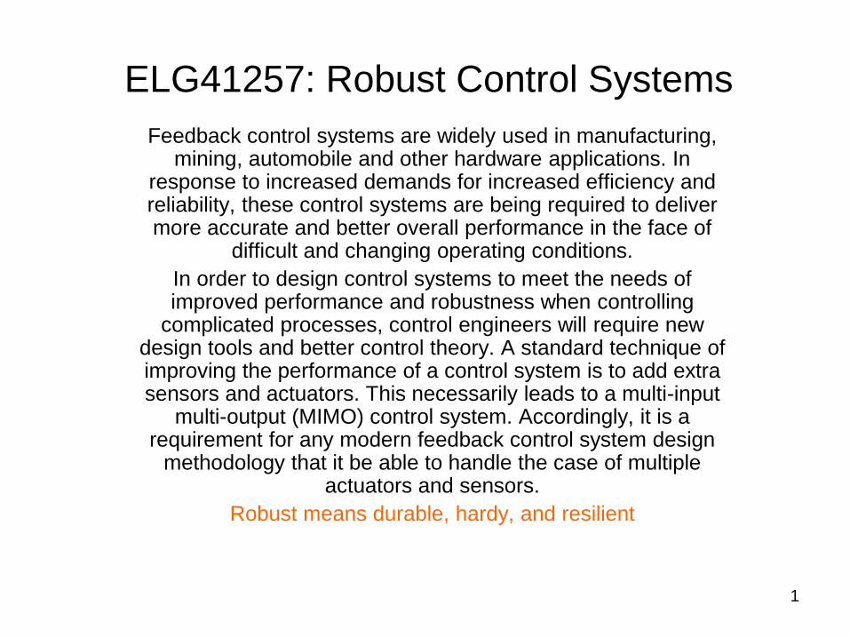
ELG41257: Robust Control Systems

Feedback control systems are widely used in manufacturing, mining, automobile and other hardware applications. In

response to increased demands for increased efficiency and reliability, these control systems are being required to deliver more accurate and better overall performance in the face of

difficult and changing operating conditions.

In order to design control systems to meet the needs of improved performance and robustness when controlling

complicated processes, control engineers will require new design tools and better control theory. A standard technique of improving the performance of a control system is to add extra sensors and actuators. This necessarily leads to a multi-input

multi-output (MIMO) control system. Accordingly, it is a requirement for any modern feedback control system design

methodology that it be able to handle the case of multiple actuators and sensors.

Robust means durable, hardy, and resilient

2

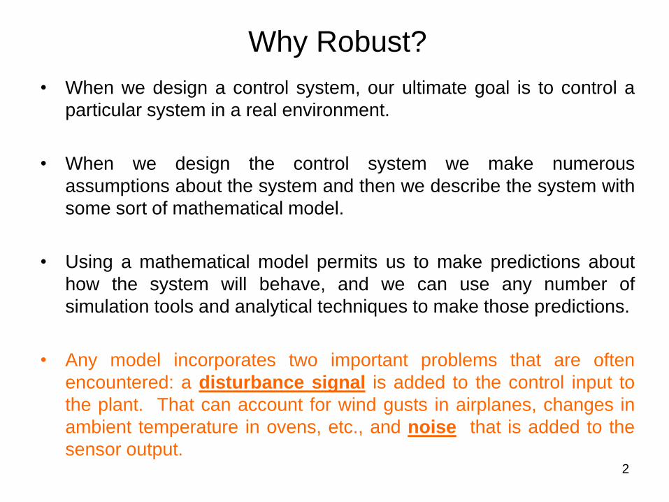
Why Robust?

• When we design a control system, our ultimate goal is to control a

particular system in a real environment.

• When we design the control system we make numerous

assumptions about the system and then we describe the system with

some sort of mathematical model.

• Using a mathematical model permits us to make predictions about

how the system will behave, and we can use any number of

simulation tools and analytical techniques to make those predictions.

• Any model incorporates two important problems that are often

encountered: a disturbance signal is added to the control input to

the plant. That can account for wind gusts in airplanes, changes in

ambient temperature in ovens, etc., and noise that is added to the

sensor output.

3

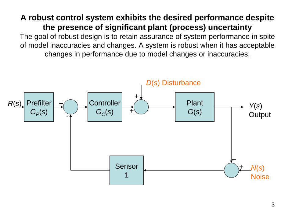
A robust control system exhibits the desired performance despite

the presence of significant plant (process) uncertainty The goal of robust design is to retain assurance of system performance in spite

of model inaccuracies and changes. A system is robust when it has acceptable

changes in performance due to model changes or inaccuracies.

D(s) Disturbance

R(s) Prefilter

GP(s)

Controller

GC(s)

Plant

G(s)

Sensor

1

+

-

+

+

+ +

Y(s)

Output

N(s)

Noise

4

Why Feedback Control Systems?

• Decrease in the sensitivity of the system to variation in

the parameters of the process G(s).

• Ease of control and adjustment of the transient

response of the system.

• Improvement in the rejection of the disturbance and

noise signals within the system.

• Improvement in the reduction of the steady-state error

of the system

5

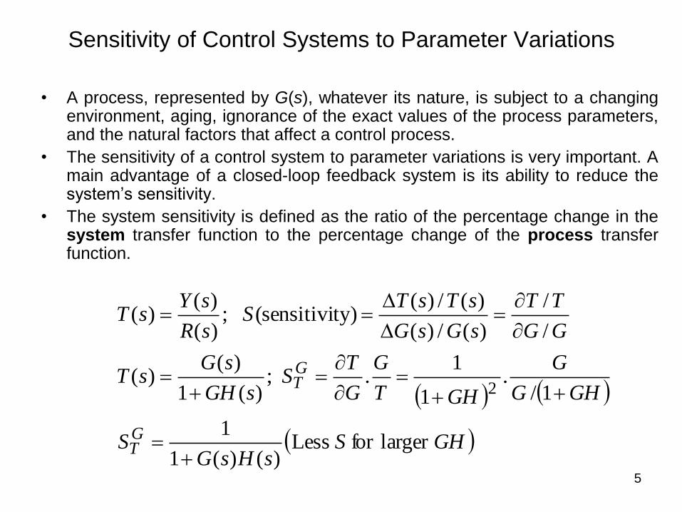
Sensitivity of Control Systems to Parameter Variations

• A process, represented by G(s), whatever its nature, is subject to a changing environment, aging, ignorance of the exact values of the process parameters, and the natural factors that affect a control process.

• The sensitivity of a control system to parameter variations is very important. A main advantage of a closed-loop feedback system is its ability to reduce the system’s sensitivity.

• The system sensitivity is defined as the ratio of the percentage change in the system transfer function to the percentage change of the process transfer function.

GHSsHsG

S

GHG

G

GHT

G

G

TS

sGH

sGsT

GG

TT

sGsG

sTsTS

sR

sYsT

GT

GT

larger for Less)()(1

1

1/.

1

1. ;

)(1

)()(

/

/

)(/)(

)(/)(ty)(sensitivi ;

)(

)()(

2

6

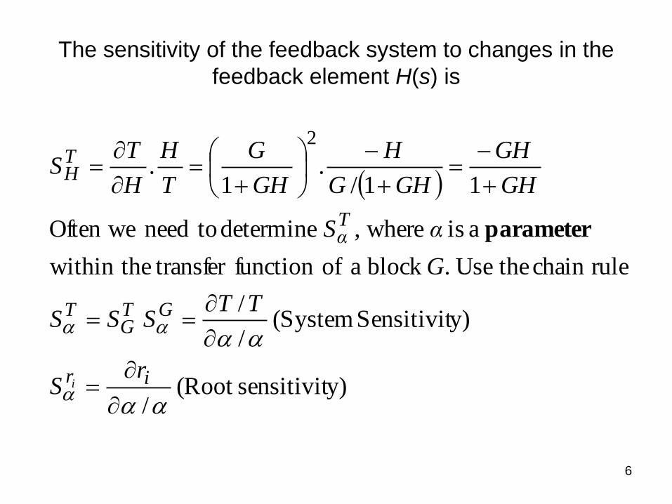
The sensitivity of the feedback system to changes in the

feedback element H(s) is

y)sensitivit(Root /

y)Sensitivit (System /

/

rulechain the Use.block a offunction transfer within the

a is where, determine toneed Often we

11/.

1.

2

ir

GTG

T

Tα

TH

rS

TTSSS

G

αS

GH

GH

GHG

H

GH

G

T

H

H

TS

i

parameter

7

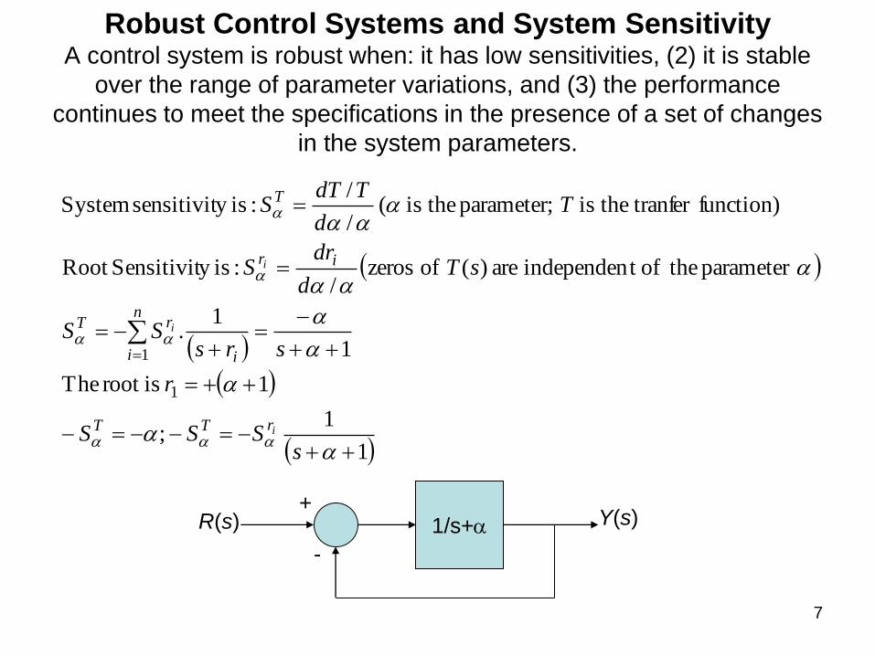
Robust Control Systems and System Sensitivity A control system is robust when: it has low sensitivities, (2) it is stable

over the range of parameter variations, and (3) the performance

continues to meet the specifications in the presence of a set of changes

in the system parameters.

1

1 ;

1 isroot The

1

1.

parameter theoft independen are )( of zeros/

:isy SensitivitRoot

function) tranfer theis parameter; theis ( /

/ :isy sensitivit System

1

1

sSSS

r

srsSS

sTd

drS

Td

TdTS

i

i

i

rTT

i

n

i

rT

ir

T

1/s+ +

-

R(s) Y(s)

8

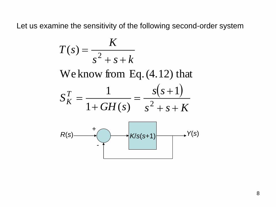
Let us examine the sensitivity of the following second-order system

Kss

ss

sGHS

kss

KsT

TK

2

2

1

)(1

1

that(4.12) Eq. from know We

)(

K/s(s+1) +

-

R(s) Y(s)

9

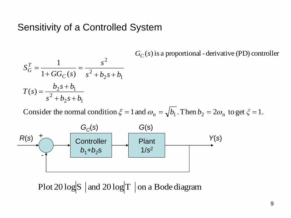
Sensitivity of a Controlled System

1.get to2Then . and 1condition normal heConsider t

)(

)(1

1

n21n

122

12

122

2

ξbb

bsbs

bsbsT

bsbs

s

sGGS

C

TG

diagram Bode aon Tlog 20 and Slog 20Plot

Controller

b1+b2s

Plant

1/s2

R(s) +

-

Y(s)

G(s) GC(s)

controller (PD) derivative-alproportion a is )(sGC

10

Disturbance Signals in a Feedback Control System

• Another important effect of feedback in a control system is the control

and partial elimination of the effect of disturbance signal.

• A disturbance signal is an unwanted input signal that affects the

system output signal. Electronic amplifiers have inherent noise

generated within the integrated circuits or transistors; radar systems

are subjected to wind gusts; and many systems generate all kinds of

unwanted signals due to nonlinear elements.

• Feedback systems have the beneficial aspects that the effect of

distortion, noise, and unwanted disturbances can be effectively

reduced.

11

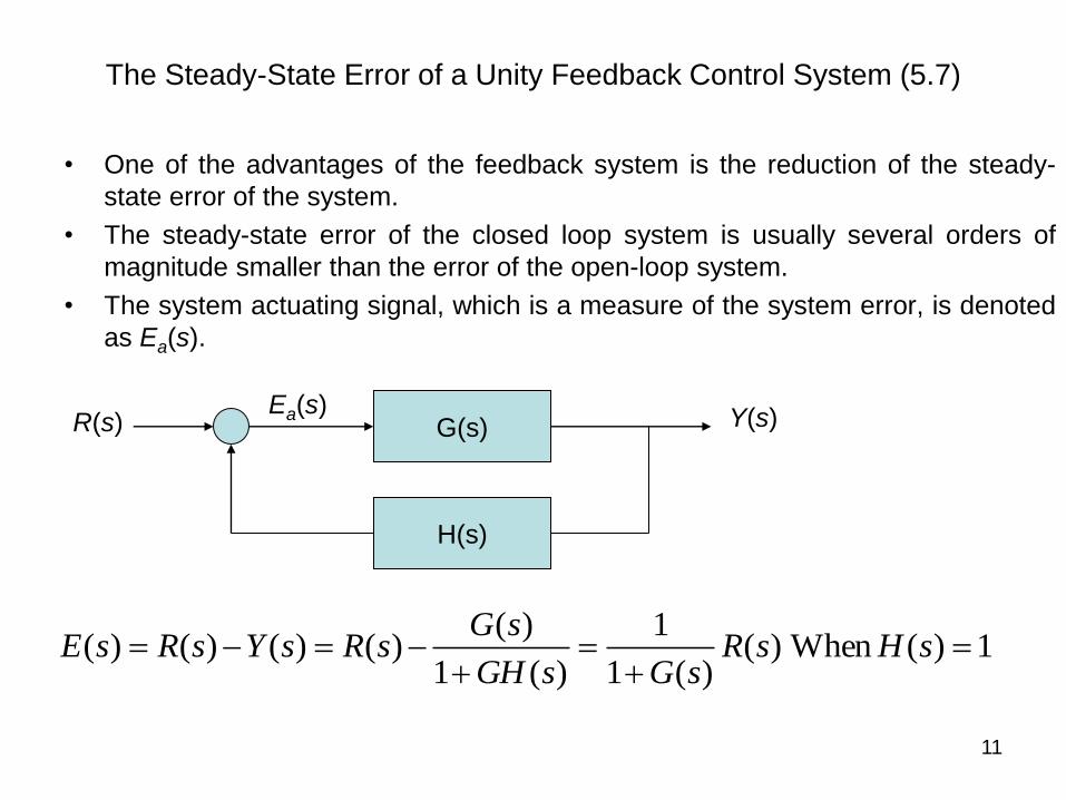
The Steady-State Error of a Unity Feedback Control System (5.7)

• One of the advantages of the feedback system is the reduction of the steady-

state error of the system.

• The steady-state error of the closed loop system is usually several orders of

magnitude smaller than the error of the open-loop system.

• The system actuating signal, which is a measure of the system error, is denoted

as Ea(s).

G(s)

H(s)

Y(s) R(s) Ea(s)

1)( When )()(1

1

)(1

)()()()()(

sHsR

sGsGH

sGsRsYsRsE

12

Compensator • A feedback control system that provides an optimum performance

without any necessary adjustments is rare. Usually it is important to compromise among the many conflicting and demanding specifications and to adjust the system parameters to provide suitable and acceptable performance when it is not possible to obtain all the desired specifications.

• The alteration or adjustments of a control system in order to provide a suitable performance is called compensation.

• A compensator is an additional component or circuit that is inserted into control system to compensate for a deficient performance.

• The transfer function of a compensator is designated as GC(s) and the compensator may be placed in a suitable location within the structure of the system.

13

Root Locus Method

• The root locus is a powerful tool for designing and analyzing

feedback control systems.

• It is possible to use root locus methods for design when two or three

parameters vary. This provides us with the opportunity to design

feedback systems with two or three adjustable parameters. For

example the PID controller has three adjustable parameters.

• The root locus is the path of the roots of the characteristic equation

traced out in the s-plane as a system parameter is changed.

• Read Table 7.2 to understand steps of the root locus procedure.

• The design by the root locus method is based on reshaping the root

locus of the system by adding poles and zeros to the system open

loop transfer function and forcing the root loci to pass through

desired closed-loop poles in the s-plane.

14

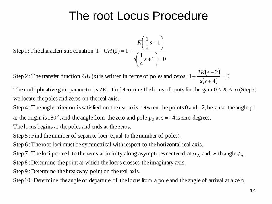
The root Locus Procedure

zero. aat arrival of angle theand pole a from locus theof departure of angle theDetermine :10 Step

axis. real on thepoint breakway theDetermine :9 Step

axis.imaginary thecrosses locus heat which tpoint theDetermine :8 Step

. angle with and at centered asymptotes alonginfinity at zeros the toproceed loci The :7 Step

axis. real horizontal therespect to with lsymmetrica bemust lociroot The :6 Step

poles). ofnumber the to(equal loci separate ofnumber theFind :5 Step

zeros. at the ends and poles at the begins locus The

degrees. zero is 4- sat pole and zero thefrom angle theand ,180 isorigin at the

p1 angle thebecause 2,- and 0 points ebetween th axis real on the satisfied iscriterion angle The :4 Step

axis. real on the zeros and poles thelocate we

(Step3) 0gain for the roots of locus thedetermine To .2 isparameter gain tivemultiplica The

04

221 :zeros and poles of in terms written is )(function transfer The :2 Step

014

1

12

1

1)(1equation sticcharacteri The :1 Step

AA

2o

p

KK

ss

sKsGH

ss

sK

sGH

15

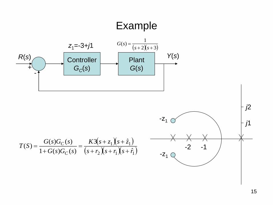
Example

32

1)(

sssG

Controller

GC(s)

Plant

G(s)

R(s) Y(s)

- +

z1=-3+j1

-1 -2

-z1

-z1

112

11

ˆ

ˆ3

)()(1

)()()(

rsrsrs

zszsK

sGsG

sGsGST

C

C

j1

j2

16

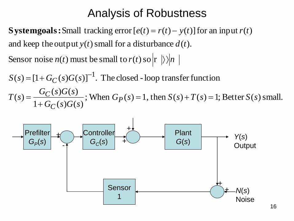
Analysis of Robustness

Prefilter

GP(s)

Controller

GC(s)

Plant

G(s)

Sensor

1

+

-

+

+

+ +

Y(s)

Output

N(s)

Noise

small. )(Better ;1)()( then 1,)( When ;)()(1

)()()(

function transfer loop-closed The .)]()(1[)(

r so )( tosmall bemust )( noiseSensor

).( edisturbanc afor small )(output thekeep and

)(input an for )]()()([error trackingSmall

1

sSsTsSsGsGsG

sGsGsT

sGsGsS

ntrtn

tdty

trtytrte

PC

C

C

:goals System

17

The Design of Robust Control Systems

• The design of robust control systems is based on two tasks: determining the structure of the controller and adjusting the controller’s parameters to give an optimal system performance. This design process is done with complete knowledge of the plant. The structure of the controller is chosen such that the system’s response can meet certain performance criteria.

• One possible objective in the design of a control system is that the controlled system’s output should exactly reproduce its input. That is the system’s transfer function should be unity. It means the system should be presentable on a Bode gain versus frequency diagram with a 0-dB gain of infinite bandwidth and zero phase shift. Practically, this is not possible!

• Setting the design of robust system requires us to find a proper compensator, GC(s) such that the closed-loop sensitivity is less than some tolerance value.

18

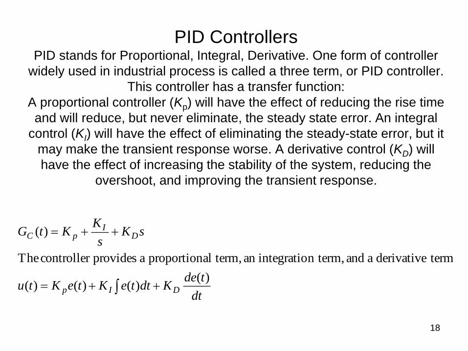
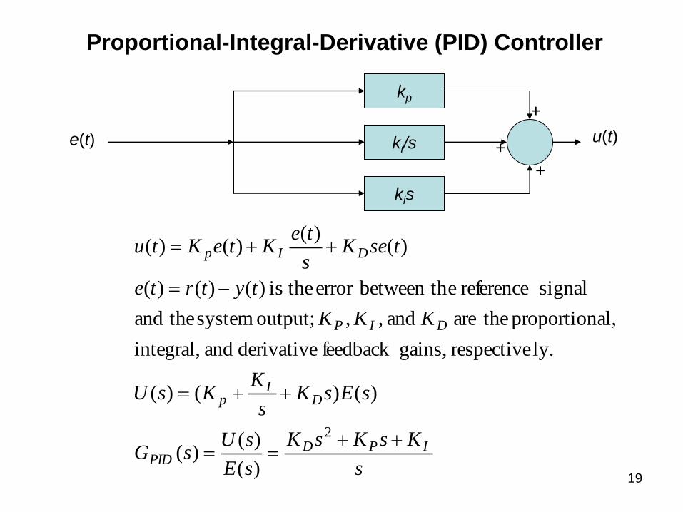
PID Controllers PID stands for Proportional, Integral, Derivative. One form of controller

widely used in industrial process is called a three term, or PID controller.

This controller has a transfer function:

A proportional controller (Kp) will have the effect of reducing the rise time

and will reduce, but never eliminate, the steady state error. An integral

control (KI) will have the effect of eliminating the steady-state error, but it

may make the transient response worse. A derivative control (KD) will

have the effect of increasing the stability of the system, reducing the

overshoot, and improving the transient response.

dt

tdeKdtteKteKtu

sKs

KKtG

DIp

DI

pC

)()()()(

termderivative a and n term,integratioan term,alproportion a provides controller The

)(

19

Proportional-Integral-Derivative (PID) Controller

kp

ki/s

kis

+

+

+

e(t) u(t)

s

KsKsK

sE

sUsG

sEsKs

KKsU

KKK

tytrte

tseKs

teKteKtu

IPDPID

DI

p

DIP

DIp

2

)(

)()(

)()()(

ly.respective gains,feedback derivative and integral,

al,proportion theare and ,, output; system theand

signal reference ebetween therror theis )()()(

)()(

)()(

20

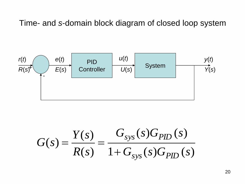
Time- and s-domain block diagram of closed loop system

PID

Controller System

r(t) e(t) u(t)

-

+ R(s) E(s) U(s)

y(t)

Y(s)

)()(1

)()(

)(

)()(

sGsG

sGsG

sR

sYsG

PIDsys

PIDsys

21

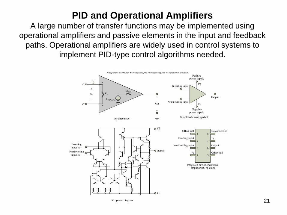
PID and Operational Amplifiers A large number of transfer functions may be implemented using

operational amplifiers and passive elements in the input and feedback

paths. Operational amplifiers are widely used in control systems to

implement PID-type control algorithms needed.

22

Figur

e 8.5

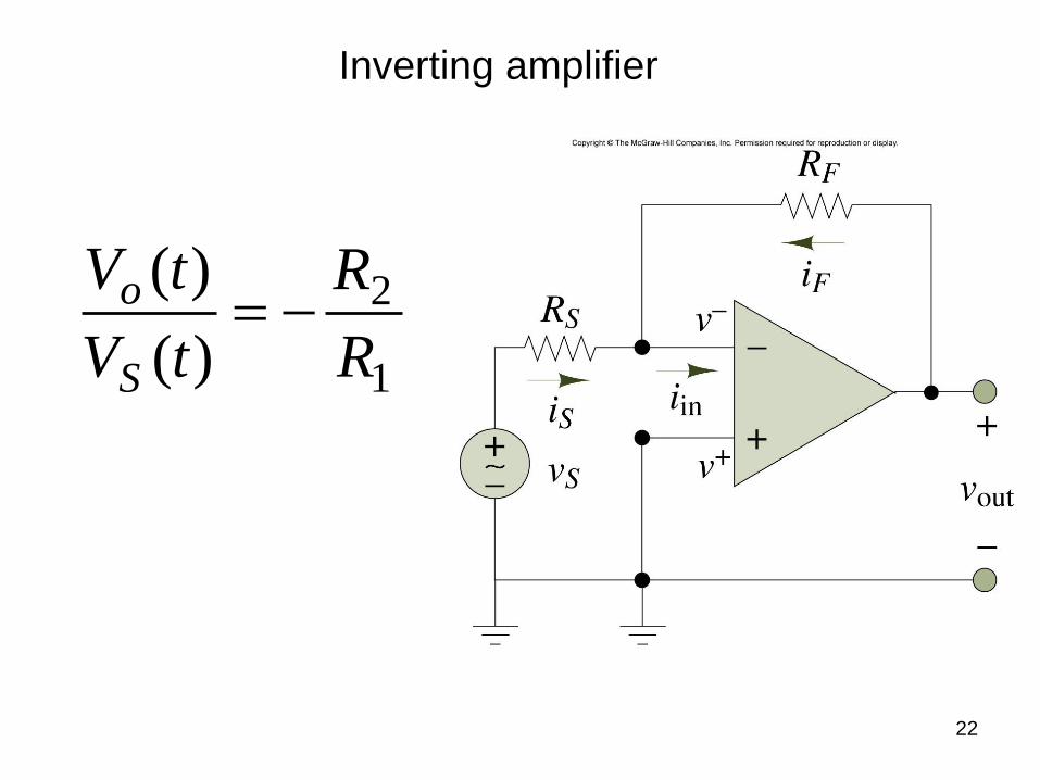
Inverting amplifier

1

2

)(

)(

R

R

tV

tV

S

o

23

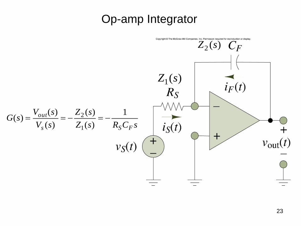
Figure

8.30

Op-amp Integrator

sCRsZ

sZ

sV

sVsG

FSs

out 1

)(

)(

)(

)()(

1

2

)(1 sZ

)(2 sZ

24

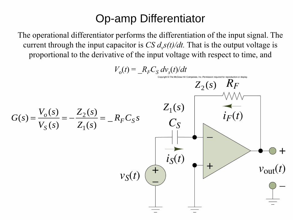
Figure 8.35

Op-amp Differentiator

The operational differentiator performs the differentiation of the input signal. The

current through the input capacitor is CS dvs(t)/dt. That is the output voltage is

proportional to the derivative of the input voltage with respect to time, and

Vo(t) = _RFCS dvs(t)/dt

sCRsZ

sZ

sV

sVsG SF

S

o _)(

)(

)(

)()(

1

2

)(2 sZ

)(1 sZ

25

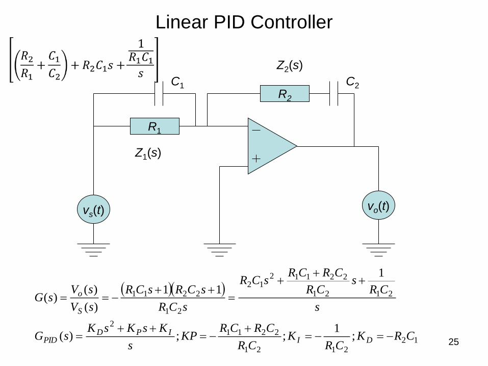
Linear PID Controller

vo(t)

R1

R2

vs(t)

C1 C2

Z2(s)

Z1(s)

122121

22112

2121

2211212

21

2211

;1

;;)(

1

11

)(

)()(

CRKCR

KCR

CRCRKP

s

KsKsKsG

s

CRs

CR

CRCRsCR

sCR

sCRsCR

sV

sVsG

DIIPD

PID

S

o

26

Tips for Designing a PID Controller When you are designing a PID controller for a given system, follow the

following steps in order to obtain a desired response.

• Obtain an open-loop response and determine what needs to be improved

• Add a proportional control to improve the rise time

• Add a derivative control to improve the overshoot

• Add an integral control to eliminate the steady-state error

• Adjust each of Kp, KI, and KD until you obtain a desired overall response.

• It is not necessary to implement all three controllers (proportional, derivative, and integral) into a single system, if not needed. For example, if a PI controller gives a good enough response, then you do not need to implement derivative controller to the system.

27

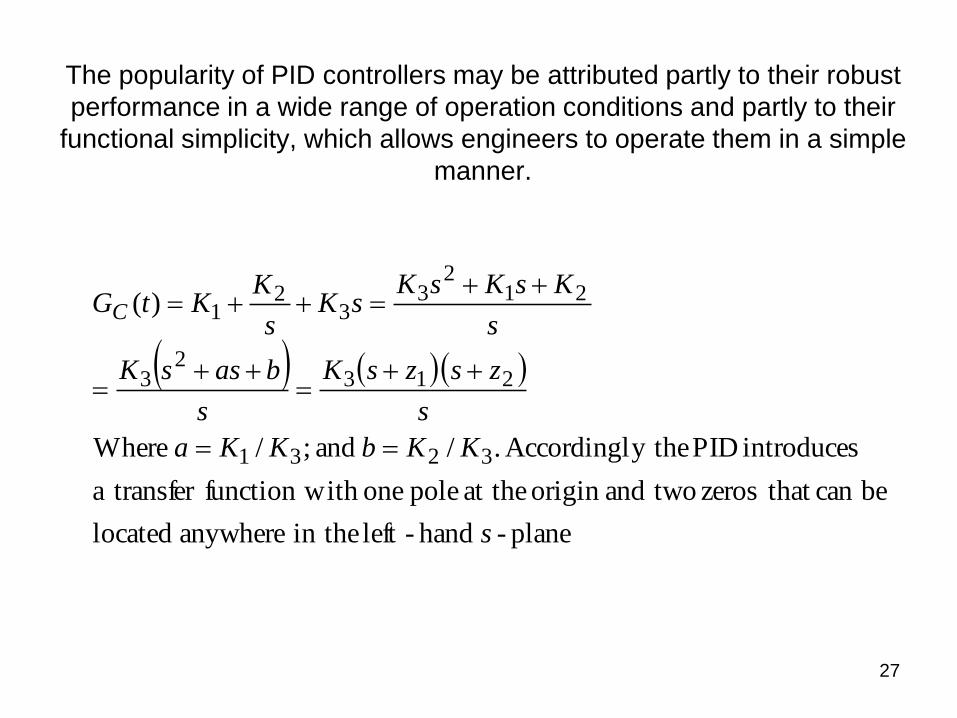
The popularity of PID controllers may be attributed partly to their robust

performance in a wide range of operation conditions and partly to their

functional simplicity, which allows engineers to operate them in a simple

manner.

plane- hand-left in the anywhere located

becan that zeros twoandorigin at the pole oneith function w transfer a

introduces PID y theAccordingl ./ and ;/ Where

)(

3231

2132

3

212

33

21

s

KKbKKa

s

zszsK

s

bassK

s

KsKsKsK

s

KKtGC

28

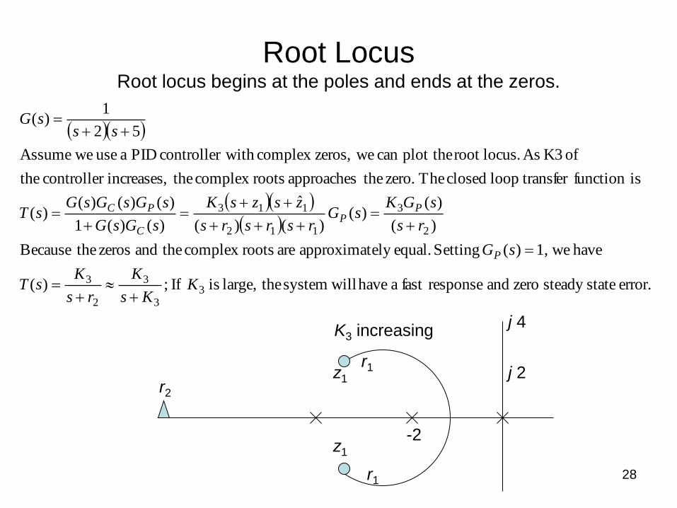
Root Locus Root locus begins at the poles and ends at the zeros.

error. statesteady zero and responsefast a have willsystem thelarge, is If ;)(

have we1,)( Setting equal.ely approximat are rootscomplex theand zeros theBecause

)(

)()(

)()(

ˆ

)()(1

)()()()(

isfunction transfer loop closed The zero. theapproaches rootscomplex theincreases, controller the

of K3 As locus.root plot thecan wezeros,complex with controller PID a use weAssume

52

1)(

33

3

2

3

2

3

112

113

KKs

K

rs

KsT

sG

rs

sGKsG

rsrsrs

zszsK

sGsG

sGsGsGsT

sssG

P

PP

C

PC

-2

r2

j 2

j 4 K3 increasing

z1

z1

r1

r1

29

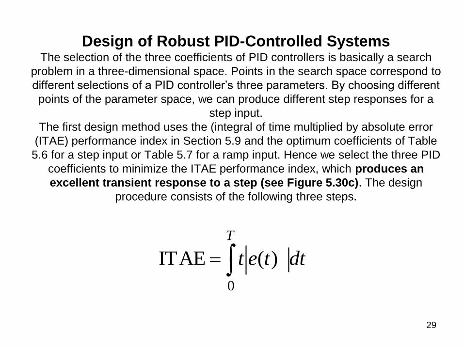
Design of Robust PID-Controlled Systems The selection of the three coefficients of PID controllers is basically a search

problem in a three-dimensional space. Points in the search space correspond to

different selections of a PID controller’s three parameters. By choosing different

points of the parameter space, we can produce different step responses for a

step input.

The first design method uses the (integral of time multiplied by absolute error

(ITAE) performance index in Section 5.9 and the optimum coefficients of Table

5.6 for a step input or Table 5.7 for a ramp input. Hence we select the three PID

coefficients to minimize the ITAE performance index, which produces an

excellent transient response to a step (see Figure 5.30c). The design

procedure consists of the following three steps.

dttet

T

0

)(ITAE

30

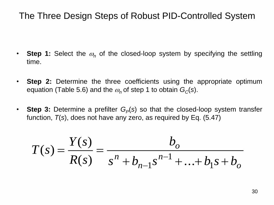
The Three Design Steps of Robust PID-Controlled System

• Step 1: Select the n of the closed-loop system by specifying the settling

time.

• Step 2: Determine the three coefficients using the appropriate optimum

equation (Table 5.6) and the n of step 1 to obtain GC(s).

• Step 3: Determine a prefilter GP(s) so that the closed-loop system transfer

function, T(s), does not have any zero, as required by Eq. (5.47)

on

nn

o

bsbsbs

b

sR

sYsT

1

11 ...)(

)()(

31

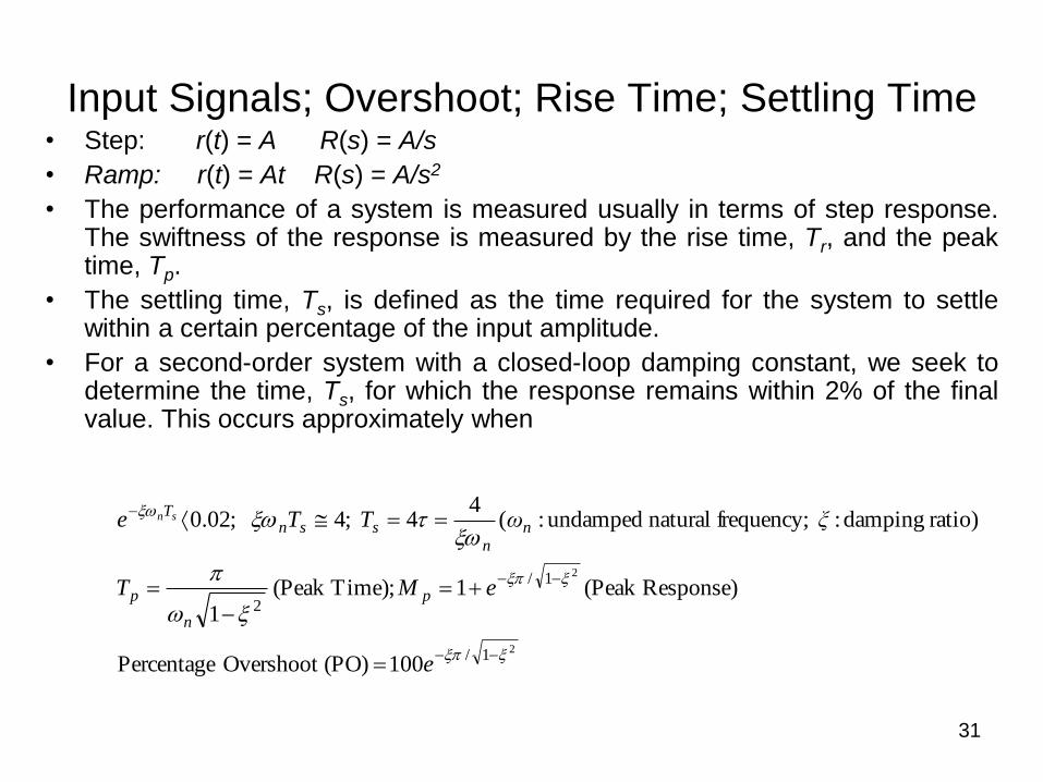
Input Signals; Overshoot; Rise Time; Settling Time • Step: r(t) = A R(s) = A/s

• Ramp: r(t) = At R(s) = A/s2

• The performance of a system is measured usually in terms of step response. The swiftness of the response is measured by the rise time, Tr, and the peak time, Tp.

• The settling time, Ts, is defined as the time required for the system to settle within a certain percentage of the input amplitude.

• For a second-order system with a closed-loop damping constant, we seek to determine the time, Ts, for which the response remains within 2% of the final value. This occurs approximately when

2

2

1/

1/

2

100 (PO)Overshoot Percentage

Response)(Peak 1 Time);(Peak 1

ratio) damping : frequency; natural undamped :(4

4 ;4 ;02.0

e

eMT

ξωTTe

p

n

p

nn

ssnTsn

Effects of Poles and Zeros

• The response of a dominantly second order system is

sped up by an additional zero and is slowed down by an

additional pole.

• In the dominantly second-order system the added closed

loop zero also has the important effect of increasing the

amount of oscillation in the system while an added

closed loop pole has the effect of decreasing the amount

of oscillation.

• Added forward path zeros and added forward path poles

have an opposite effect on the overshoot.

• A forward path pole which is too close to the origin may

turn the closed loop system unstable.

32

33

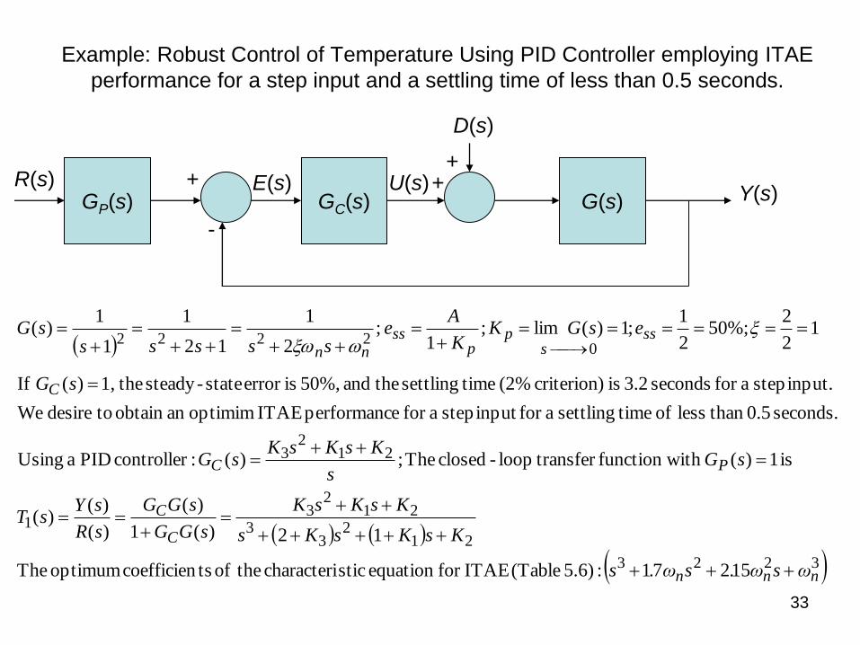
Example: Robust Control of Temperature Using PID Controller employing ITAE

performance for a step input and a settling time of less than 0.5 seconds.

3223

212

33

212

31

212

3

02222

15271 :5.6) (Table ITAEfor equation sticcharacteri theof tscoefficien optimum The

12)(1

)(

)(

)()(

is 1)(ith function w transfer loop-closed The;)( :controller PID a Using

seconds. 0.5 than less of timesettling afor input step afor eperformanc ITAE optimiman obtain todesire We

input. step afor seconds 3.2 is criterion) (2% timesettling theand 50%, iserror state-steady the1,)( If

12

2%;50

2

1;1)( lim;

1 ;

2

1

12

1

1

1)(

nnn

C

C

PC

C

sss

pp

ss

nn

ωsω.sω.s

KsKsKs

KsKsK

sGG

sGG

sR

sYsT

sGs

KsKsKsG

sG

esGKK

Ae

ssssssG

R(s) GP(s) GC(s) G(s) Y(s)

D(s)

+ + +

-

U(s) E(s)

34

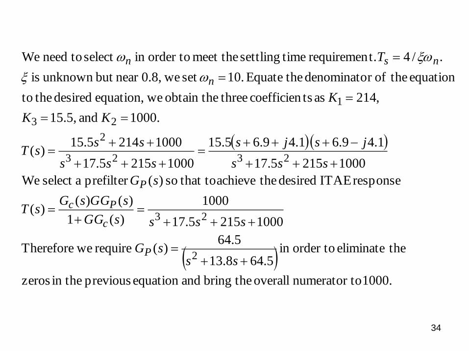
1000. tonumerator overall thebring andequation previous in the zeros

theeliminate order toin 5.648.13

5.64)( require weTherefore

10002155.17

1000

)(1

)()()(

response ITAE desired theachieve that toso )(prefilter aselect We

10002155.17

1.49.6 1.49.65.15

10002155.17

10002145.15)(

1000. and 15.5,

,214 as tscoefficien threeobtain the weequation, desired theto

equation theofr denominato theEquate 10.set we0.8,near but unknown is

./4 t.requiremen timesettling meet the order toin select toneed We

2

23

2323

2

23

1

sssG

ssssGG

sGGsGsT

sG

sss

jsjs

sss

sssT

KK

K

T

P

c

Pc

P

n

nsn

35

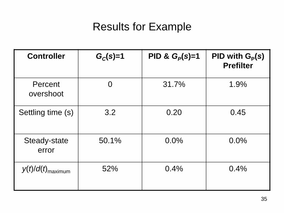
Results for Example

Controller GC(s)=1 PID & GP(s)=1 PID with GP(s)

Prefilter

Percent

overshoot

0 31.7% 1.9%

Settling time (s) 3.2 0.20 0.45

Steady-state

error

50.1% 0.0% 0.0%

y(t)/d(t)maximum 52% 0.4% 0.4%

36

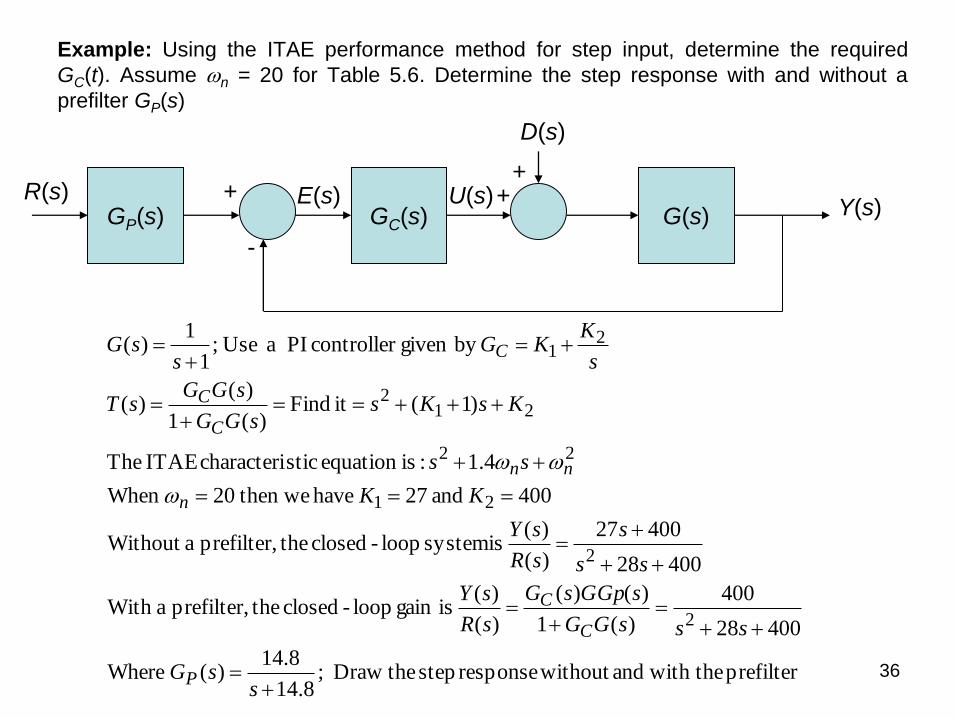
Example: Using the ITAE performance method for step input, determine the required

GC(t). Assume n = 20 for Table 5.6. Determine the step response with and without a

prefilter GP(s)

prefilter with theand without response step theDraw ;8.14

8.14)( Where

40028

400

)(1

)()(

)(

)( isgain loop-closed theprefilter, aWith

40028

40027

)(

)( is system loop-closed theprefilter, aWithout

400 and 27 have then we20When

4.1 :isequation sticcharacteri ITAE The

)1(it Find )(1

)()(

by given controller PI a Use;1

1)(

2

2

21

22

212

21

ssG

sssGG

sGGpsG

sR

sY

ss

s

sR

sY

KK

ss

KsKssGG

sGGsT

s

KKG

ssG

P

C

C

n

nn

C

C

C

GP(s) GC(s) G(s) Y(s)

D(s)

+ + +

-

U(s) E(s) R(s)

37

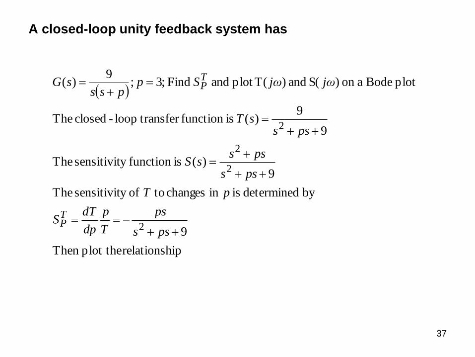
A closed-loop unity feedback system has

iprelationsh plot theThen

9

by determined is in changes to ofy sensitivit The

9)( isfunction y sensitivit The

9

9)( isfunction transfer loop-closed The

plot Bode aon )S( and )T(plot and Find ;3;9

)(

2

2

2

2

pss

ps

T

p

dp

dTS

pT

pss

psssS

psssT

jωjωSppss

sG

TP

TP

38

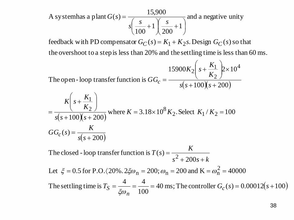
10000012.0)( controller The ms; 40100

44 is timesettling The

40000K and 200 200;2 20%. P.O.for 0.5Let

200)( isfunction transfer loop-closed The

200)(

100/Select .1018.3 where200100

200100

10215900

isfunction transfer loop-open The

ms. 60 than less is timesettling theand 20% than less is step a toovershoot the

that so )(Design .)(r compensato PDith feedback w

unity negative a and

1200

1100

900,15)(plant a has systemA

2nnn

2

21282

1

4

2

12

21

ssGT

kss

KsT

ss

KsGG

KKKKsss

K

KsK

sss

K

KsK

GG

sGsKKsG

sss

sG

cn

S

c

c

CC

39

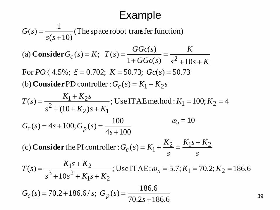
Example

6.1862.70

6.186)( ;/6.1862.70)(

6.186;2.70;7.5 :ITAE Use;10

)(

)( :controller PI the )c(

1004

100)(;1004)(

4;100 :method ITAE Use;)10(

)(

)( :controller PD (b)

73.50)( ;73.50 ;702.0 4.5%; For

10)(1

)()( ;)( (a)

function)sfer robot tran space (The)10(

1)(

21

2123

21

2121

21

122

21

21

2

ssGssG

KKKsKss

KsKsT

s

KsK

s

KKsG

ssGssG

KKKsKs

sKKsT

sKKsG

sGcKPO

Kss

K

sGGc

sGGcsTKsG

sssG

pc

n

c

pc

c

c

Consider

Consider

Consider

n = 10

40

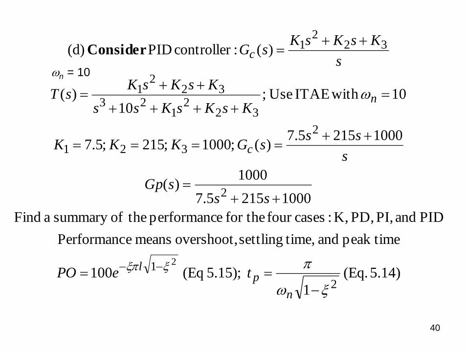
5.14) (Eq.

1

;5.15) (Eq 100

peak time and time,settling overshoot, means ePerformanc

PID and PI, PD, K, :casesfour for the eperformanc theofsummary a Find

10002155.7

1000)(

10002155.7)( ;1000 ;215 ;5.7

10 with ITAE Use;10

)(

)( :controller PID (d)

2

1

2

2

321

322

123

322

1

322

1

2

n

pl

c

n

c

tePO

sssGp

s

sssGKKK

KsKsKss

KsKsKsT

s

KsKsKsGConsider

n = 10

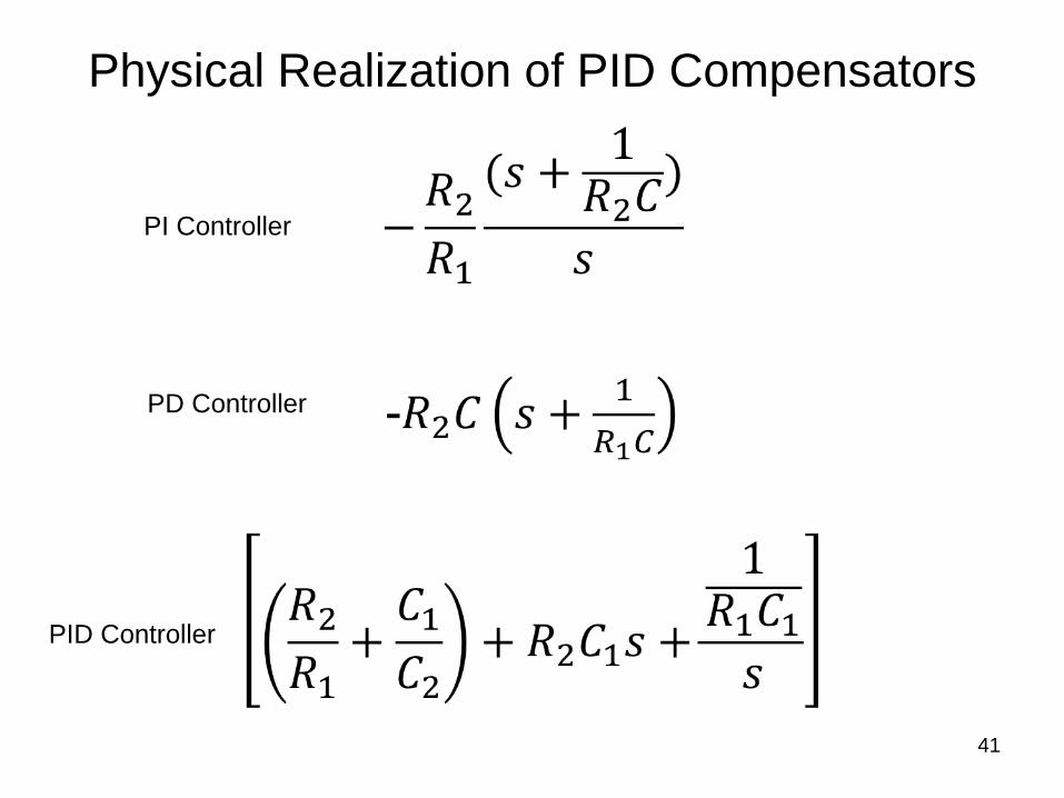
Physical Realization of PID Compensators

41

PI Controller

PD Controller

PID Controller