Robust Control of Flexible Motion Systems: A Literature … · Summary This literature study focusses on robust control of ﬂexible motion systems. Traditionally, motion systems

Robust Control of FlexibleMotion Systems:A Literature Study

S.L.H. Verhoeven

DCT Report 2009.006

APT536-09-6288

Supervisors: Dr. ir. J.J.M. van Helvoort†

Dr. ir. M.M.J. van de Wal†

Ir. T.A.E. Oomen‡

Prof.ir. O.H. Bosgra‡

† Philips Applied Technologies

Mechatronics Program

Drives and Control Group

‡ Eindhoven University of Technology

Department of Mechanical Engineering

Dynamics and Control Technology Group

Eindhoven, January 2009

Summary

This literature study focusses on robust control of flexible motion systems. Traditionally,motion systems are designed such that the frequency of the dominant flexible dynamics ishigh compared to the required bandwidth. As many independent single-input single-outputcontrollers as degrees-of-freedom are then used to control the rigid body modes of the system,where both the feedback and feedforward controller design is based on the input/outputbehaviour of the plant. However, increased throughput requirements lead to lighter motionsystems, causing the dominant flexible dynamics to shift towards the required bandwidth. Asa consequence, actuator forces will deform the body relative to the tensionless equilibrium.The traditional geometric relation between measurement information on the one hand anddesired position information on the other hand is then no longer valid. The actual systemperformance may thus be limited by internal deformations that are not represented well inthe input/output model. This is the essence of “beyond-rigid-body control”.

The first part of this literature study gives an overview of the theory behind H∞-optimisationand µ-synthesis. These norm-based controller design techniques are considered relevant forbeyond rigid body control, due to a variety of reasons. First, these techniques allow for anexplicit distinction between performance variables and measured variables. Second, they areable to explicitly account for system uncertainty. Information of high-frequency dynamics isnot accurately available and putting a lot of control effort into controlling these dynamicsis undesired. Third, the control problem in H∞-optimisation and µ-synthesis is solved in auniform way, regardless of the number of inputs and outputs. Therefore, it is easier to dealwith - possibly non-square - plants with many actuators and sensors.

The second part discusses literature on actively controlling the internal dynamics of a body.A common approach is the explicitly control a set of modes, while neglecting the other modes.In literature, it is shown that this method often works well for relatively simple systems, e.g.,beams or thin plates, but it is believed that for more complex systems the application ofmodal control is less straightforward and may not work. One of the reasons for this, is the socalled “spillover” effect, which is the effect of the neglected modes on the closed-loop system.By adding extra actuators (over-actuation) and sensors (over-sensing) to a flexible motionsystem, it is possible to explicitly control the flexible modes. Several control structures existin which over-actuation (and over-sensing) can be applied. It can be used for either feedfor-ward, feedback, or feedback and feedforward simultaneously. Which control structure leadsto the best result depends on the system, the actuator/sensor configuration, the performancemeasure and the external disturbances. In order to achieve the best performance the work ofthe control engineer should therefore not be limited to merely controller design, but shouldalso include the placement of the actuators and sensors.

i

Abbreviations

ARE Algebraic Riccati EquationBRB Beyond Rigid BodyDOF Degree-Of-FreedomDGKF Doyle, Glover, Khargonekar, FrancisDISO Double-Input Single-OutputEMC Efficient Modal ControlFEM Finite Element ModelFRF Frequency Response FunctionGM Gain MarginHCARE H∞ Controller Algebraic Riccati EquationHCARE H∞ Filter Algebraic Riccati EquationIMSC Independent Modal Space ControlIC Integrated CircuitILC Iterative Learning ControlIO Input/OutputLFT Linear Fractional TransformationLHP Left Half PlaneLPV Linear Parameter VaryingLQG Linear Quadratic GaussianMIMO Multi-Input Multi-OutputMM Modulus MarginNP Nominal PerformanceNS Nominal StabilityPM Phase MarginRHP Right Half PlaneRP Robust PerformanceRS Robust StabiiltySISO Single-Input Single-OutputSSV Structured Singular ValueTFM Transfer Function Matrix

iii

Contents

Summary i

Abbreviations iii

Contents v

1 Introduction 1

1.1 Background . . . . . . . . . . . . . . . . . . . . . . . . . . . . . . . . . . . . . 1

1.2 Project motivation and problem formulation . . . . . . . . . . . . . . . . . . . 2

1.3 Outline of the Report . . . . . . . . . . . . . . . . . . . . . . . . . . . . . . . 3

1.4 Overview of common terms in literature . . . . . . . . . . . . . . . . . . . . . 4

1.5 Global literature overview . . . . . . . . . . . . . . . . . . . . . . . . . . . . . 5

2 Robust Control 7

2.1 Introduction . . . . . . . . . . . . . . . . . . . . . . . . . . . . . . . . . . . . . 7

2.2 Benefits of advanced control . . . . . . . . . . . . . . . . . . . . . . . . . . . . 7

2.3 General control configuration . . . . . . . . . . . . . . . . . . . . . . . . . . . 8

2.3.1 Including weights in the general control configuration . . . . . . . . . 9

2.3.2 Including uncertainty in the general control configuration . . . . . . . 9

2.4 Control problems . . . . . . . . . . . . . . . . . . . . . . . . . . . . . . . . . . 11

2.5 Nominal Performance . . . . . . . . . . . . . . . . . . . . . . . . . . . . . . . 12

2.6 Robust Stability and Robust Performance . . . . . . . . . . . . . . . . . . . . 14

2.6.1 Modelling uncertainty . . . . . . . . . . . . . . . . . . . . . . . . . . . 14

2.6.2 Robust stability . . . . . . . . . . . . . . . . . . . . . . . . . . . . . . 16

2.6.3 Motivation for the structured singular value . . . . . . . . . . . . . . . 18

v

vi Contents

2.6.4 Robust performance . . . . . . . . . . . . . . . . . . . . . . . . . . . . 19

2.6.5 Restatement of control problems . . . . . . . . . . . . . . . . . . . . . 20

2.7 Solutions to the H∞ optimal control problem . . . . . . . . . . . . . . . . . . 20

2.7.1 DGKF solution to H∞ control problem . . . . . . . . . . . . . . . . . 20

2.7.2 µ-Synthesis . . . . . . . . . . . . . . . . . . . . . . . . . . . . . . . . . 22

2.8 Feedforward design . . . . . . . . . . . . . . . . . . . . . . . . . . . . . . . . . 23

2.9 Summary and conclusions . . . . . . . . . . . . . . . . . . . . . . . . . . . . . 23

3 Robust control for an ASML wafer scanner 25

3.1 Introduction . . . . . . . . . . . . . . . . . . . . . . . . . . . . . . . . . . . . . 25

3.2 Control goal and control structure . . . . . . . . . . . . . . . . . . . . . . . . 25

3.3 Plant modelling . . . . . . . . . . . . . . . . . . . . . . . . . . . . . . . . . . . 27

3.4 Performance quantification . . . . . . . . . . . . . . . . . . . . . . . . . . . . 27

3.4.1 Weighting filters for scaling . . . . . . . . . . . . . . . . . . . . . . . . 28

3.4.2 Weighting filters for loop shaping . . . . . . . . . . . . . . . . . . . . . 28

3.4.3 Weighting filters to account for power spectra . . . . . . . . . . . . . . 30

3.5 Uncertainty quantification . . . . . . . . . . . . . . . . . . . . . . . . . . . . . 31

3.6 Results . . . . . . . . . . . . . . . . . . . . . . . . . . . . . . . . . . . . . . . . 31


4 Vibration control of flexible structures 35

4.1 Introduction . . . . . . . . . . . . . . . . . . . . . . . . . . . . . . . . . . . . . 35

4.2 System description . . . . . . . . . . . . . . . . . . . . . . . . . . . . . . . . . 36

4.2.1 Distributed parameter system . . . . . . . . . . . . . . . . . . . . . . . 36

4.2.2 Nodal models . . . . . . . . . . . . . . . . . . . . . . . . . . . . . . . . 37

4.2.3 Modal models . . . . . . . . . . . . . . . . . . . . . . . . . . . . . . . . 38

4.2.4 Relevance of modal analysis . . . . . . . . . . . . . . . . . . . . . . . . 41

4.3 Modal control . . . . . . . . . . . . . . . . . . . . . . . . . . . . . . . . . . . . 42

4.3.1 Independent modal space control . . . . . . . . . . . . . . . . . . . . . 42

4.3.2 Coupled control . . . . . . . . . . . . . . . . . . . . . . . . . . . . . . . 43

4.3.3 Spillover . . . . . . . . . . . . . . . . . . . . . . . . . . . . . . . . . . . 45

4.3.4 Example: spillover effect . . . . . . . . . . . . . . . . . . . . . . . . . . 46

Contents vii

4.4 Robust control for large space structures . . . . . . . . . . . . . . . . . . . . . 50

4.4.1 Problem formulation . . . . . . . . . . . . . . . . . . . . . . . . . . . . 50

4.4.2 Modelling uncertainty and performance specification . . . . . . . . . . 51

4.4.3 Tradeoffs between robustness and performance . . . . . . . . . . . . . 52

4.4.4 Control of flexible modes in the controller crossover region . . . . . . . 54


5 Control of flexible motion systems 57

5.1 Introduction . . . . . . . . . . . . . . . . . . . . . . . . . . . . . . . . . . . . . 57

5.2 Three aspects of controller design . . . . . . . . . . . . . . . . . . . . . . . . . 58

5.2.1 First aspect: control structure . . . . . . . . . . . . . . . . . . . . . . 58

5.2.2 Second aspect: actuator/sensor position . . . . . . . . . . . . . . . . . 60

5.2.3 Third aspect: performance definition . . . . . . . . . . . . . . . . . . . 61

5.3 Control of flexible motion systems without over-actuation . . . . . . . . . . . 63

5.3.1 Conventional controller design . . . . . . . . . . . . . . . . . . . . . . 64

5.3.2 Advanced controller design . . . . . . . . . . . . . . . . . . . . . . . . 66

5.3.3 Actuator/sensor placement . . . . . . . . . . . . . . . . . . . . . . . . 67

5.3.4 Interpretation of transmission zeros . . . . . . . . . . . . . . . . . . . 68

5.4 Control of flexible motion systems with over-actuation . . . . . . . . . . . . . 69

5.4.1 Internal and external over-actuation . . . . . . . . . . . . . . . . . . . 69

5.4.2 Double-input single-output (DISO) . . . . . . . . . . . . . . . . . . . . 70

5.4.3 Internal over-actuation . . . . . . . . . . . . . . . . . . . . . . . . . . . 71


6 Conclusions and recommendations 77

6.1 Conclusions . . . . . . . . . . . . . . . . . . . . . . . . . . . . . . . . . . . . . 77

6.2 Recommendations . . . . . . . . . . . . . . . . . . . . . . . . . . . . . . . . . 79

A Interpretation of transmission zeros 81

Bibliography 87

Chapter 1

Introduction

1.1 Background

Philips Applied Technologies has a long history of research on advanced control for highprecision motion systems. Several topics, such as multivariable control, H∞-optimisation, µ-synthesis, LPV control, and ILC have been examined for high-precision and high-throughputstages. This research has especially been done for ASML, which is a leading company in themarket for chip manufacturing machines, i.e., wafer scanners. These machines are used forthe production of Integrated Circuits (ICs). ICs are produced on a silicon wafer (200 mm- 300 mm diameter) by a photolithographic process. An important mechanical componentof the wafer scanner is the wafer stage that positions the silicon wafer with respect to theimaging optics. Because very fine patterns have to be produced on the wafer, a positionaccuracy in the order of nanometers and microradians is required.

High-accuracy stages are nowadays controlled in six Degrees-Of-Freedom (DOFs): the threerigid body translations and rotations. The design of the control loops is mostly based on sixactuators and sensors, to independently control the six rigid body DOFs. To keep controldesign simple, Single-Input Single-Output (SISO) controllers are common practice, despitethe Multi-Input Multi-Output (MIMO) nature of the problem. The design of the feedback andfeedforward controllers is usually based on the plant Input/Output (IO) behaviour. Based onthe IO plant model, controller design aims at creating suitable (closed-loop) transfer functionbehaviour.

However, the actual performance of a motion system is not necessarily represented well by theIO behaviour of the plant and the corresponding closed-loop transfer functions that ratherrepresent servo performance. This situation occurs if internal plant dynamics become relevantthat is not directly sensed, as for a wafer stage [36]. The actual system performance is interms of the positioning of that part of the silicium wafer that is subject to the light exposure.The servo performance is only an approximation of this true goal, since it is based on laserinterferometer data (measured at the edges of the wafer stage) that is transferred via a sensortransformation into coordinates of the area on the wafer subject to exposure. However, thesensor transformation assumes the wafer stage to be a rigid body system and hence thepossible contribution of internal dynamics (flexible modes) is neglected. Because various

1

2 Introduction

forces (actuation, disturbances, gravity) act on a body with finite stiffness, the body willexhibit internal deformations relative to the tensionless equilibrium. The traditional geometricrelation between measurement information on the one hand and desired position informationon the other hand is then no longer valid. A similar reasoning applies to the actuator side,where internal deformations refute the validity of the traditional actuator transformation thatis derived on the basis of a rigid-body plant model. The actual system performance may thusbe limited by modal deformations that are not represented in the IO model used for feedbackand feedforward controller design.

1.2 Project motivation and problem formulation

Because of the fierce competition in the IC market, it is desirable to put more and smallertransistors on a single IC and to increase the throughput of the wafer scanner. ASML istherefore faced with the industrial challenge to build bigger and lighter stages, while at thesame time the requirements on the servo error and throughput become ever demanding.With this tendency, it will eventually become necessary to much more rigorously address thepresence of flexible modes in the control system design. Explicitly taking into account theinternal plant dynamics (besides the usual IO behaviour) in the controller design providesopportunities to improve the actual system performance of mechatronic stages. At this mo-ment, studying the following control design freedom is considered worthwhile in the contextof “beyond-rigid-body (BRB) control”:

• Over-actuation: The usage of more actuators than free rigid body DOFs, to enablethe possibility to actively control the internal flexible modes, instead of the present -rather passive - approach of limiting the undesired effect of these modes as much aspossible.

• Over-sensing: The usage of more sensors than rigid body DOFs, to explicitly sensethe internal flexible modes or to at least improve the observability of such modes andhence to enable the possibility to improve the controller design in the face of flexiblemodes.

• Vibration control of structures: Using “over-actuation” and “over-sensing” to ex-plicitly control the flexible modes of a motion system is in some way equivalent tocontrolling a system without rigid body modes, e.g., a structure. Since a lot of researchhas already been done in that field, it is believed that valuable information can beobtained from it.

• Explicit distinction between sensed vs. performance variables: Exploiting theexplicit distinction that can be made in the controller design between the variables thatare sensed (y) and the variables that represent the actual system performance (z). Asdiscussed above, for wafer stages z could be in terms of the positioning of the spot onthe wafer subject to exposure, while y would rather be in terms of the spots on the edgeof the wafer measured by the interferometer, see Figure 1.1. The internal dynamicsbetween these “performance” and “sensed” locations may cause a relevant deviationof the servo accuracy in y vs. the exposure accuracy in z. The so-called generalised

1.3 Outline of the Report 3

standard plant set-up, which is depicted in Figure 1.2 and is also used in norm-basedcontroller design, can be used to make an explicit distinction between y and z in thecontroller design, thereby providing the potential to design more effective controllers.

K P

Pzz

uy

G

Figure 1.1: Standard feedback configuration with an explicit distinction between sensed andperformance variables.

Considering the control design freedom listed above, the goal of this literature study can bedivided into two parts:

• Examine norm-based controller design and its applicability to an ASML wafer scanner.

• Examine the control of flexible modes in structures and in flexible motion systems.

K

G

w z

u y

Figure 1.2: General control configuration.

1.3 Outline of the Report

The report is organised as follows. Chapter 2 discusses H∞-optimisation and µ-synthesis.Both techniques can be used to design MIMO controllers for a wide variety of system. Itis expected that these norm-based controller designs lead to better results for the problemat hand than classical loop shaping methods due to a variety of reasons. For example, dueto the explicit distinction between the performance and sensed variables and because of thesystematic way of dealing with a large number of inputs and outputs.

4 Introduction

In Chapter 3 it is shown how H∞-optimisation and µ-synthesis can be used to create MIMOcontrollers for ASML wafer stages. In [50] it is shown that these types of controllers can beregarded as feasible successors for the standard SISO controllers that are currently used.

Chapter 4 focusses on vibration control in flexible structures. Flexible structures are inthis report regarded as systems without rigid body modes. Although flexible structures arevery different from wafer stages and traditional motion systems, i.e., no rigid body modes,similarities occur in the form of closely spaced flexible modes and the uncertainty in thehigh-frequency modes.

Chapter 5 focusses on vibration control in motion systems. The concept of using more ac-tuators and sensors than rigid body modes is introduced, which boils down to adding moreactuators and sensors to explicitly control the flexible modes. The benefit of over-actuationand over-sensing is shown for a simple “free-free” beam system.

In Chapter 6 the main results and conclusions are summarised and recommendations aregiven for further research.

1.4 Overview of common terms in literature

In literature, different terms are often used to describe similar things. In this section, a shortoverview is given of some common terms that are considered relevant in the context of BRBcontrol.

• Flexible mode or vibration mode: A “flexible mode” refers to a periodic motion thatis physically possible in the absence of any external influence and in which the elastic dis-placement w(p, t) at position p and time t all move in unison, i.e., all displacements passthrough zero simultaneously and they all attain their maxima simultaneously, see [28].In this report the term flexible mode is used.

• Rigid bode mode: Similar as a flexible mode, but instead of a periodic motion itdescribe a direction of displacement without flexible deformation. Hence, the corre-sponding natural frequency is zero. Structural analysts often ignore this mode, becausethere is no deformation involved. However, for the control engineer this mode is crucial,since it allows the structure or system to be moved or track a command.

• Mode Shape: Modes shapes can refer to flexible modes and rigid body modes.

• System: It is quite difficult - or maybe impossible - to give one good description of a“system” since a system can be almost anything. In this literature study and in thecontext of BRB control, the term system is used to describe a physical product withunalterable properties. For example, a wafer stage, a car, or a two-mass-spring system.In other contexts, the term “system” can mean different things.

• Structure or flexible structure: A “structure” is a type of system in which rigid bodymodes are not considered relevant for control purposes or do not exist. To avoid confu-sion. the term “flexible structure” should then ideally be used to describe a structurethat has no rigid body modes. However, in literature both terms are used in parallel.

1.5 Global literature overview 5

• Flexible system: A system in which flexible modes are present and not negligibleunder normal operation. In theory, all systems have a finite stiffness and can thereforebe regarded flexible. However, not all systems contain flexible modes that are relevantduring normal operation.

• Flexible motion system: A motion system in which the flexible modes are relevantduring normal operation.

• Intelligent structure: This term often refers to (large) structures in which control isapplied. For example, a building that is able to withstand earthquakes.

• Active vibration control: Control effort aimed at controlling the flexible modes ina system. Rigid body modes are not present or are not considered relevant. Hence,the term “structural vibration control” is also used. Passive vibration control has thesame goal as active vibration control, but the goal is basically achieved by modifyingthe structure, e.g., vibration isolation, or adding local springs and masses, instead ofusing actuators and sensors, see [46].

• Vibration damping: Often the control law in active vibration control focusses ondamping the flexible modes and this is referred to as “vibration damping”. Anotherpossibility is to compensate for a flexible mode.

1.5 Global literature overview

In this section, a compact overview is given of the literature that - at this moment - isconsidered relevant in the context of norm-based control and controlling flexible systems.Since it is impossible to give a complete overview, only the most well known literature sourcesare used. Not all literature listed below is used for this literature study and the literature isdivided into four groups:

• Robust control. A lot of books and papers have been written about classical androbust control theory. Two well known books are the book of Skogestad and Postleth-waite [48] and the book of Zhou et al. [54]. The former focusses on practical feedbackcontrol and the latter more on system theory.

• Modal control. Two books about the modal system description are [18, 35, 40].Although these books emphasise the advantages of the modal system description, somedrawbacks of the modal description exist and are presented in a paper of Hughes,see [28]. The concept of modal control is also covered in [18, 40], but a lot moreliterature is available, see, e.g., [8, 34, 47]. In [47] the concept of Efficient ModalControl is introduced, i.e., using displacement or energy content of each mode as weightto determine the feedback control force.

• Robust control of flexible modes. A lot of literature is available on robust controlof flexible structures, due to the difficulties in accurate modelling of flexible structures.A comprehensive and recent overview of the application of H∞-Optimisation and µ-synthesis in controlling flexible modes is given in [29]. Also, a tutorial is presented for

6 Introduction

designing H∞-based controllers for a smart plate, i.e., a plate equipped with actuatorsand sensors. Most of the literature discussed in [29] is quite similar. It mainly concernsthe creation of SISO or MIMO H∞-based controllers with collocated actuators andsensors, for controlling a flexible beam, plate, or antenna-like structure. The onlydifferences occur in the combined work of Halim and Moheimani [23, 24, 35], wherea spatial performance norm is minimised, i.e., performance is required at an infinitelylarge set of points. The work done in [43] is also different, because actuators andsensors are used in a non-collocated setting. Unfortunately, no motivation is given forthis choice.

In [32], the performance of a H∞-based controller is compared to traditional velocityfeedback and LQG control. The main conclusion is that “simple” velocity feedbackoutperforms the H∞-based controller. This is opposite to the results in [43], where theH∞-based controller is superior. A possible explanation for this big difference is thatthe H∞ control problem is not formulated well.

In [11], a method is proposed to design control laws based on H∞-optimisation, for flex-ible structures with closely spaced modes and collocated actuators and sensors. More-over, the solution presented avoids calculation of the Algebraic Riccati Equations, seeChapter 2, so an explicit solution for the controller is obtained.

In [21, 26, 27], robustness is achieved in a different way. Only parametric uncertainty isconsidered and stability of the closed loop system, including the parametric uncertainty,is proven by using Lyapunov stability theory. In [27], the topic is active robust shapecontrol of flexible structures and the authors propose a method to control the shape ofthe structure under the influence of disturbances. For example, maintaining a certainoptimal wing cross section during flights. Controlling the shape of a structure can notbe done without controlling the flexible modes of a structure. Hence, it is consideredrelevant.

In the early 90’s a lot of work has been done by G.J. Balas, see [1, 3–7]. In this workthe flexible modes of a structure, called the “Caltech experimental flexible structure”,are suppressed by using µ-synthesis. Actuators and sensors are used in a non-collocatedsetting and the structure has closely spaced flexible modes and uncertainty in the higherfrequency modes.

At Eindhoven University of Technology and Philips, research has been done on control-ling flexible modes in motion systems. Recent work that is considered relevant for thisliterature study is the work done by M. Schneiders, see [44–46] and J.W. van Winger-den [53]. Both authors discuss the use of extra sensors and actuators to explicitly controlthe flexible modes in a motion system.

• Actuator and sensor selection. The problem of choosing a good location for theactuators and sensors (possibly non-collocated) in a flexible motion system is brieflyintroduced in some of the literature about robust control of flexible modes, see, e.g., [43,44, 53]. The topic of actuator/sensor selection is investigated more thoroughly in [22,25, 31, 42, 44, 52].

Chapter 2

Robust Control

2.1 Introduction

As mentioned in the introduction, wafer stages are currently controlled by six SISO controllers,despite the MIMO nature of the problem. This chapter first briefly discusses H∞-optimisationand µ-synthesis as a type of MIMO control. In literature, H∞-optimisation and µ-synthesisare extensively studied in various areas of engineering. For more details the reader is advisedto study [37, 48, 50, 51]. A more comprehensive overview is given by [14, 54, 55].

2.2 Benefits of advanced control

SISO feedback controllers are usually designed using manual loop shaping. Based on Bodediagrams and Nyquist plots of the open-loop transfer function, parameters are tuned suchthat properties like BandWidth (BW), Phase Margin (PM), and Gain Margin (GM) are met.Often, this results in a series connection of low-order filters, like integrators, lead-lag filters,notches, and low-pass filters. This conventional design has some disadvantages:

• Loop shaping is usually performed in an open-loop setting. The open-loop gain shouldbe large at low frequencies to meet the performance requirements (reference trackingand disturbance rejection) and small at high frequencies, in order to not amplify mea-surement noise. In between, the open loop gain is approximately one. The point wherethe open-loop gain crosses the 0 [dB] line from above for the first time, is defined asthe BW of the system.1 At the bandwidth the phase should be large enough (phasemargin) to be stable. However, it is more natural to do loop shaping in a closed loopfashion, since in the end it is the closed-loop performance that counts.

• It is not guaranteed that the best controller is found by manually shaping the open-loop, since this is subject to the experience of the control engineer. This drawback

1This is the definition of BW that is used in this report. In literature this point is often referred to ascrossover frequency and the bandwidth is defined in closed-loop; either in the sensitivity, S, or complementarysensitivity, T .

7

8 Robust Control

could be resolved by formulating the control problem as an optimisation problem witha guaranteed global optimum.

• If the control problem becomes more complicated, loop shaping becomes hard or almostimpossible. For instance, if MIMO plants with strong interaction are considered, if thenumber of actuators and sensors increases, or if there are performance requirements onmultiple closed-loop transfer functions.

• There is no straightforward manner to account for modelling errors and uncertainty inthe plant model. High-frequency roll-off can be used to achieve some robustness againsthigh-frequency resonance modes and unmodelled dynamics, but a more sophisticatedapproach to robust controller design is desirable.

• The measured and regulated variables need to be the same. The performance objectivesneed thus be stated in terms of variables that can be measured.

The disadvantages listed above are, at least in theory, resolved by controller design usingH∞-optimisation and µ-synthesis.2 Both topics are briefly described in the remainder ofthis chapter. A disadvantage of these more advanced controller design techniques is theneed for a plant model, whereas for conventional controller design a measured FrequencyResponse Function (FRF) is sufficient. In addition, using six individual SISO controllers3 ismore transparent, and hence simpler. Control engineers are more familiar with manual loopshaping and terms like phase-, gain- and Modulus Margin (MM).

2.3 General control configuration

Most advanced controller design techniques, like H∞-optimisation and µ-synthesis, make useof the general control configuration as depicted in Figure 2.1. Herein, G is the generalisedstandard plant4 and K is the controller to be designed. The regulated variables, i.e., thevariables to be kept small, are stacked in the vector z. Typical signals that are often includedin z are control actions and servo errors. The measured output signals that are used ascontroller input are collected in vector y, which implies that the control objective does nothave to be stated in terms of measured signals. The vector w contains the exogenous inputs,e.g., disturbances, sensor noise, but also reference trajectories. The controller output signalsare stacked in vector u. Note y and u do not have to be of the same size, i.e., the controllerdoes not have to be a square matrix.

The generalised standard plant can be represented as:

[zy

]=

[G11 G12

G21 G22

] [wu

], (2.1)

or as a state-space representation:

2The term synthesis us used rather that design to stress that it is a more formalised approach.3This is also called multiloop SISO control4Sometimes G is referred to as “standard plant” or “augmented (standard) plant”. In this report the term

“standard plant” refers to the physical standard plant, i.e., the plant without weighting filters.

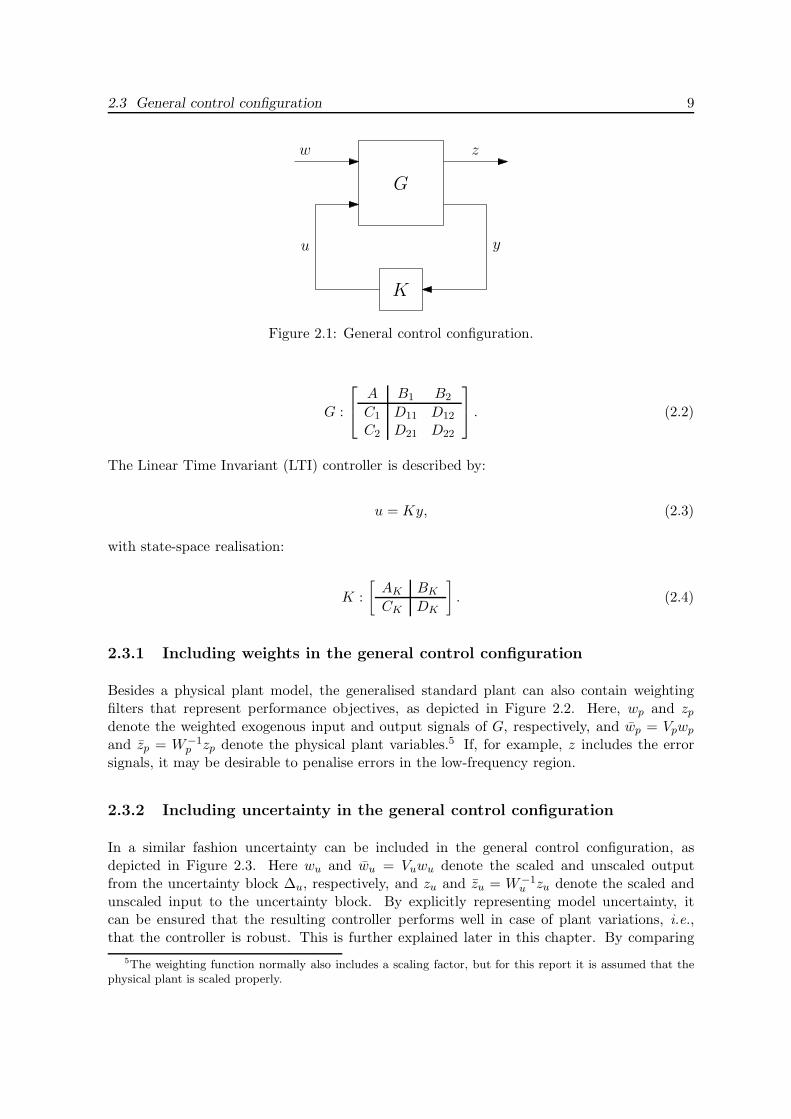
2.3 General control configuration 9

K

G

w z

u y

Figure 2.1: General control configuration.

G :

A B1 B2

C1 D11 D12

C2 D21 D22

. (2.2)

The Linear Time Invariant (LTI) controller is described by:

u = Ky, (2.3)

with state-space realisation:

K :

[AK BK

CK DK

]. (2.4)

2.3.1 Including weights in the general control configuration

Besides a physical plant model, the generalised standard plant can also contain weightingfilters that represent performance objectives, as depicted in Figure 2.2. Here, wp and zp

denote the weighted exogenous input and output signals of G, respectively, and wp = Vpwp

and zp = W−1p zp denote the physical plant variables.5 If, for example, z includes the error

signals, it may be desirable to penalise errors in the low-frequency region.

2.3.2 Including uncertainty in the general control configuration

In a similar fashion uncertainty can be included in the general control configuration, asdepicted in Figure 2.3. Here wu and wu = Vuwu denote the scaled and unscaled outputfrom the uncertainty block ∆u, respectively, and zu and zu = W−1

u zu denote the scaled andunscaled input to the uncertainty block. By explicitly representing model uncertainty, itcan be ensured that the resulting controller performs well in case of plant variations, i.e.,that the controller is robust. This is further explained later in this chapter. By comparing

5The weighting function normally also includes a scaling factor, but for this report it is assumed that thephysical plant is scaled properly.

10 Robust Control

G

K

Vp Wpwp zp zpwp

G

M

yu

Figure 2.2: General control configuration with performance weights.

Figure 2.2 and Figure 2.3 it can be seen that the setup is similar, except that the exogenousvariables are separated in two groups: variables related to performance (subscript p) anduncertainty-related signals (subscript u).

The closed-loop system can then be written as z = Mw:

[zu

zp

]=

[M11 M12

M21 M22

] [wu

wp

]. (2.5)

G

K

Vp Wpwp zp zpwp

∆u

wu zuVu Wu

yu

zuwu

G

M

Figure 2.3: General control configuration with performance weights and model uncertainty.

Remark 2.1 In case of vector valued signals wp, wu, zp, and zu, Vp, Vu, Wp, and Wu become

2.4 Control problems 11

matrices. Since the off-diagonal components of these matrices are difficult to interpret, theweighting matrices are often chosen to be diagonal.

2.4 Control problems

Various goals can be pursued in the controller design. The following four control problemsare distinguished in [48]:

• Nominal Stability (NS): The closed-loop system is stable in the absence of modeluncertainty. NS is always required. NS is further explained in [48].

• Nominal Performance (NP): The closed-loop system is stable and it achieves theperformance specifications in the absence of model uncertainty. NP implies NS.

• Robust Stability (RS): The closed-loop system is stable in the presence of a certainclass of model uncertainties. RS implies NS

• Robust Performance (RP): The closed-loop system is stable and it achieves theperformance specifications in the presence of model uncertainty. RP implies NS, NP,and RS.

Several definitions of stability exist in literature. Here Definition 4.4 of [48] is used:

Definition 2.1 A system is (internally) stable if none of its components contain hiddenunstable modes and the injection of bounded external signals at any place in the systemresults in bounded output signals measured anywhere in the system.

Here a signal u(t) is defined to be “bounded” if there exists a constant c such that |u(t)| < cfor all t. This type of stability is also referred to as Bounded-Input Bounded-Output (BIBO)stability. The word “internally” stresses that it is not sufficient to have a stable response fromone particular input to another particular output, but require bounded signals measured atany place in the system. A continuous time linear time-invariant system x = Ax + Bu isstable if and only if all the poles pi are in the open Left Half Plane (LHP); that is, Re(pi) =Reλi(A) < 0,∀i. A system matrix with such a property is called “Hurwitz”. A system isunstable is it has any poles in the open Right Half Plane (RHP); that is Re(pi) = Reλi(A) > 0.The imaginary axis (jω-axis) is thus the stability boundary between a stable and unstableresponse. Poles on the jω-axis, like integrators and pure harmonic oscillators (s = ±jω), areunstable by Definition 2.1 given above. For example, consider a pure integrator, a constantinput co leads an unbounded output cot.

However, if stability is judged based on the response of an initial condition, different conclu-sions can be drawn for poles on the jω-axis. In [17], a system is stable if initial conditionsdecay to zero and unstable they diverge. If the system has non-repeated jω-axis poles, it issaid to be neutrally stable. For example, a single integrator results in a constant output anda pure harmonic oscillator results in an oscillating response without damping. If the systemshas repeated poles on the jω-axis, it is unstable. For example, a double integrator (massfloating in space). A non-zero initial velocity results in an unbounded position.

12 Robust Control

In the next two sections the different control problems are further elaborated. Section 2.5 dis-cusses nominal stability and nominal performance, and Section 2.6 discusses robust stabilityand robust performance.

2.5 Nominal Performance

Consider again the control problem without model uncertainty as depicted in Figure 2.1 andFigure 2.2. If the generalised standard plant G is closed with controller K, the generalisedclosed-loop system M results:

M = Fl(G,K) := G11 + G12K(I − G22K)−1G21, (2.6)

with the partitioning G as follows:

[zp

y

]=

[G11 G12

G21 G22

] [wp

u

]. (2.7)

The expressing Fl(G,K) in (2.6) is called a lower Linear Fractional Transformation (LFT)and can be read as “close G by K”. The closed-loop system M in (2.6) also contains theweighting filters Vp and Wp. The physical closed-loop system M can be defined in a similarway:

M = Fl(G,K) := G11 + G12K(I − G22K)−1G21. (2.8)

Ideally, the effect of wp on zp should be zero. Imagine, M being the sensitivity S, which is thecase if wp is the reference trajectory and zp the tracking error. In an ideal situation M = 0at all frequencies (perfect regulation), which is not possible for realistic control problems(“Waterbed effect”). Instead, the goal is to make S small at certain frequencies. To indicatein which frequencies it is important to make S small, the weighting filters Vp and Wp can beused. The controller design problem is then restated to making M = WpMVp small.

Suppose that M is a SISO system, like the sensitivity S. The gain |M(jω)| is then a naturalmeasure of smallness over the frequency domain. To come up with a scalar measure forsmallness, the H∞-norm could be used. For an asymptotically stable SISO system this normis defined as:

‖M(s)‖∞ := supω

|M(jω)|, (2.9)

with “sup” denoting the supremum. The ‖M(s)‖∞-norm thus denotes the maximum valueof the SISO transfer function M over all frequencies. So, by making proper choices for theweighting filters, the control problem amounts to designing a controller K such that the‖M‖∞-norm is bounded by a given value γ, which is usually set to 1. Controller design aimedat minimising the H∞-norm of a suitable closed-loop system is called H∞ optimisation. Othernorms than the H∞-norm can also be used, but certain properties of the H∞-norm, like the

2.5 Nominal Performance 13

sub-multiplicative property6 turn out to be very useful to incorporate uncertainty modelsthat are discussed later [37, 48].

In general, M is not a SISO system but a MIMO system. The main difference between thetwo is the presence of directions in the latter. The “gain” of M therefore depends on theparticular direction of wp. To deal with the directionality, the Singular Value Decomposition(SVD) in introduced. Consider a, possibly complex, l × m matrix M , which can also befrequency dependent. The matrix M can be factorised as follows:

M = Y ΣU∗, (2.10)

where ·∗ stands for the complex conjugate transpose. The matrices Y and U are orthonor-mal matrices of size l × l and m × m, respectively. The l × m matrix Σ contains a diagonalmatrix Σ1 of real non-negative singular values σi, arranged in descending order:

Σ =

[Σ1

0

]if l ≥ m or: Σ =

[Σ1 0

]if l ≤ m, (2.11)

where:

Σ1 = diag(σ1, σ2, . . . , σk), with: k = min(l,m). (2.12)

If wp is aligned with the ith column of U (this is called the input direction), zp will be inthe direction of the ith column of Y (output direction) and amplified by a gain σi. MatricesU and Y thus contain the information about directionality, whilst the matrix Σ contains theinformation about the “gains”. The largest gain is achieved when wp is aligned with the firstcolumn of U , which corresponds to the maximum singular value σ1. The maximum singularvalue σ1 is usually denoted by σ. For MIMO system, the H∞-norm of (2.9) can thus beadjusted to a more general form:

‖M(s)‖∞ := supω

σ(M(jω)). (2.13)

Because the H∞-norm only looks at the maximum singular value, the norm is often interpretedas a “worst-case gain”. The following definition of the H∞-norm also illustrates this character:

‖M(s)‖∞ = supwp(t)6=0

‖zp(t)‖2

‖wp(t)‖2. (2.14)

Here, wp and zp are the input and output signals of M and ‖·‖2 denotes the L2-norm of a signalthat equals the square root of the energy of a signal. The H∞-norm is thus the maximumamplification of energy of the input signal wp. From (2.14) one can easily understand thatthe H∞-norm can only be defined for systems that are asymptotically stable, since zp goes toinfinity when the system is unstable.

6This is also called “Schwartz inequality”: ‖GH‖∞ ≤ ‖G‖∞ · ‖H‖∞

14 Robust Control

2.6 Robust Stability and Robust Performance

To assess robust stability and robust performance, uncertainty models can be included inthe control configuration as depicted in Figure 2.3. Controllers resulting from NP designalso exhibit some robustness, since they have a certain phase- and gain margin. However,these properties may not be sufficient and to account for uncertainties explicitly, uncertaintymodels are incorporated in the controller design/analysis. In this section measures for robuststability and robust performance are given, but first it is explained how uncertainty can beincluded in the general control configuration.

2.6.1 Modelling uncertainty

Uncertainties are differences between the actual plant and the plant model. Various sourcesof uncertainty exist. If a plant model is known, e.g., in state space format, there is alwaysuncertainty in the parameters. This is called parametric uncertainty and it is not discussedfurther in this report. Another kind of uncertainty is dynamic uncertainty, which can arisedue to various sources:

• Model simplification: To design a controller the plant model should be kept relativelysimple. Therefore, high-frequency modes and non-linearities are often neglected.

• Production tolerances: Plants that are the same in theory, are not the same in practice.There is always some mismatch within a batch of virtually the same plants.

• Changing environmental and operating conditions: Plants are subject to wear, changesin temperature and humidity, and changing operating conditions.

• By lumping together several sources of parametric uncertainty.

Uncertainty models

There are several possibilities to quantify model uncertainty. Three possibilities are listedbelow. P∆u represents the true plant, which is subject to uncertainties and P representsthe nominal plant. Scaling filters Vu and Wu are used to normalise the magnitude of theuncertainty block ∆u to one (‖∆u‖∞ ≤ 1):

• Additive plant uncertainty, see Figure 2.4:

P∆u = P + Wu∆uVu. (2.15)

• Multiplicative uncertainty at the plant input, see Figure 2.5:

P∆u = P (I + Wu∆uVu). (2.16)

• Multiplicative uncertainty at the plant output, see Figure 2.6:

P∆u = (I + Wu∆uVu)P. (2.17)

2.6 Robust Stability and Robust Performance 15

More possibilities are possible, for example, the inverse forms of the uncertainty types listedabove. The uncertainty loop is then closed in the reverse direction.

K P

Wu Vu∆u

P∆u

zuwu

Figure 2.4: Additive plant uncertainty.

K P

Wu Vu∆u

P∆u

zuwu

Figure 2.5: Multiplicative uncertainty at the plant input.

K P

Wu Vu∆u

P∆u

zuwu

Figure 2.6: Multiplicative uncertainty at the plant output.

Sometimes the choice of what uncertainty model to use is quitte straightforward. Uncertaintyat the actuators is well modelled with input uncertainty, while uncertainty at the sensors is wellmodelled with output uncertainty. However, sometimes choosing the right type of uncertaintyis not that obvious. Besides choosing a suitable uncertainty description, a nominal plantmodel has to be chosen. In general, the uncertainty description and nominal plant modelthat lead to the least conservative controller should be used.7 In practice a nominal plant

7The term “conservatism” is used to denote that the controller is robust for candidate plants that are notlikely to arise in practice. Hence, the achieved performance might be unnecessarily limited.

16 Robust Control

model that leads to satisfactory results is found by averaging several plant FRFs over theoperating range [50].

The final step is to choose the frequency dependent weighting functions Vu(s) and Wu(s). Itis possible to use both weighting functions, but in most cases one of them is set to identityand the other is used to bound the estimated size of the uncertainty. Note that if µ-synthesisis used is does not matter whether Wu(s) or Vu(s) is set to identity, but if H∞ is used it doesmatter, [50]. The unscaled uncertainty description ∆u can be obtained for each uncertaintytype using (2.15)−(2.17) and setting both weighting functions to identity. The weightingfunction(s) has to be chosen such that it encompasses σ(∆u).

The above discussion holds for both SISO and MIMO plants. In case of a MIMO plant, it isoften desired to model uncertainty for each entry of P separately. This leads to a so calledstructured uncertainty block, which has several advantages.

Unstructured uncertainty

Imagine the plant P to be square with n inputs and n outputs. For any of the uncertaintyrepresentations in Figure 2.4−2.6, the uncertainty block has the same dimension as the plantP , i.e., n × n. Choosing weighting function Vu(s) or Wu(s) can be simplified by using scalartransfer functions vu(s) or wu(s):

Vu(s) = vu(s)In, Wu(s) = wu(s)In. (2.18)

The scaler transfer functions vu(s) and wu(s) are preferably low order and are used to en-compasses σ(∆u).

Structured uncertainty

A structured uncertainty description can be used to describe the uncertainty in each plantentry separately, leading to a potentially less conservative controller. The uncertainty blockis then not an n × n block, but a diagonal matrix of size n2 × n2 with the n2 entries of ∆u

on the main diagonal. Each entry of ∆u is now approximated by a - preferably low order -transfer function vuk

(s) or wuk(s), and these are lined up to form diagonal matrices Vu(s) and

Wu(s) of dimension n2 × n2. To make these weighting matrices compatible with the plantdimension, two permutation matrices are needed as well [50].

2.6.2 Robust stability

The RS problems boils down to finding a stabilising controller K that is stable for all plantin the set P∆u . The closed-loop system M is depicted in Figure 2.3, where M is partitionedas in (2.5). Suppose that there are no performance requirement, i.e., zp and wp are absent.The control problem is then reduced to stability problem as depicted in Figure 2.7.

Asymptotic stability can be guaranteed by the Small Gain Theorem (Theorom 4.12 in [48]):


M11

∆u

wu zu

Figure 2.7: The robust stability problem.

Theorem 2.1 Small gain theorem. Consider a system with a stable loop transfer functionL(s). Then the closed-loop system is stable if

‖L(jω)‖ < 1 ∀ω (2.19)

where ‖L‖ denotes any matrix of satisfying the submultiplicativity property ‖AB‖ ≤ ‖A‖·‖B‖.

In the robust stability problem of Figure 2.7 the (stable) loop transfer function is given byM11∆u. Since the H∞-norm satisfies the submultiplicativity property, robust stability isachieved if ‖M11∆u‖∞ < 1. Because ‖∆u‖∞ ≤ 1, RS is achieved if:

‖M11‖∞ < 1 ⇔ σ(M(jω)) < 1 ∀ω. (2.20)

Condition (2.20) is a necessary and sufficient condition for a full complex disturbance ma-trix ∆u. In the next two sections it is shown that (2.20) is overly conservative when ∆u

exhibits structure.

Remark 2.2 An important reason for using the H∞-norm to analyse robust stability is thesubmultiplicativity property. For example, an ‖H‖2-norm does not satisfy the submultiplica-tivity property is RS cannot be analysed using (2.20).

Remark 2.3 Stability can also be proven by using the generalised nyquist theorem. Theorem8.1 in [48] states that - assuming M11 and ∆u stable - the M11∆u system is asymptoticallystable if and only if

det(I − M11(jω)∆u(jω)) 6= 0, ∀ω,∀∆u. (2.21)

Introducing the spectral radius, which is defined as the maximum eigenvalue of a matrix:

ρ(L(jω)) := maxi

|λi(L(jω))| (2.22)

and under the assumption that ‖∆u‖∞ ≤ 1, (2.21) can be rewritten:

18 Robust Control

ρ(M11(jω)∆u(jω)) < 1 ∀ω ∀∆u ⇔ max∆u

ρ(M11(jω)∆u(jω)) < 1, ∀ω, (2.23)

= max∆u

σ(M11(jω)∆u(jω)) < 1, ∀ω, (2.24)

= max∆u

σ(M11(jω))σ(∆u(jω)) < 1, ∀ω, (2.25)

= max∆u

σ(M11(jω)) < 1, ∀ω. (2.26)

The step from (2.23) to (2.24) is only allowed when ∆u is an unstructured (full and complex)matrix, see Lemma 8.3 in [48].

2.6.3 Motivation for the structured singular value

As stated earlier is this report, ∆u can also be structured, i.e., ∆u is a norm-bounded (block)diagonal matrix. In many practical applications ∆u exhibits some sort of structure, e.g.,when the uncertainty at each plant entry is evaluated separately. So, in case of structureduncertainty, ∆u is only allowed to lie in a certain set ∆u that is composed of complex-valuedblocks:

∆u =diag(δu1

Ir1, . . . , δkIrk

,∆u1, . . . ,∆ul

) : δui∈ C; ∆ui

∈ Csi×ti

. (2.27)

Here, the ith scalar block has dimension ri, and the ith full uncertainty block has dimensionsi × ti. If structured uncertainty is treated as an unstructured uncertainty to evaluate RS,condition (2.20) is sufficient since σ ≤ 1. However, it is not a necessary condition anymore,since the structure of ∆u has not been taken into account.8

To take the structure into account the Structured Singular Value (SSV) is introduced ([13,39, 54]), for which the definition is given by:

µ(M) :=1

min∆u∈∆u(σ(∆u) : det(I − M11∆u) = 0)

, (2.28)

and for which the interpretation is:

Find the smallest structured ∆u (measured in terms of σ) that makes the matrix I − M11∆u

singular; then µ(M) = 1/σ.

Clearly, µ(M11) depends not only on M11 but also on the allowed structure of ∆u. This issometimes shown explicitly by using a slightly different notation: µ∆(M11). The reason whythe SSV makes use of the structure in ∆u can be made plausible by stating that scaling ofthe uncertainty matrix ∆u and closed-loop matrix M11 does not influence the stability, butchanges the maximum singular value of ∆u. For meer details, see [48, Section 8.7].

Remark 2.3 In case of unstructured uncertainties: µ(M11) = σ(M11).

8In case of structured uncertainty max∆u

ρ(M11(jω)∆u(jω)) 6= max∆u

σ(M11(jω)∆u(jω))


A similar condition as (2.20) for robust stability can now be stated for the situation where∆u exhibits structure. If M11 and ∆u are stable, and ‖∆u‖ ≤ 1, then RS is guaranteed if andonly if:

‖M11‖µ := supω

µ(M11(jω)) < 1. (2.29)

2.6.4 Robust performance

As stated earlier, Robust Performance (RP) means that the closed-loop system is stable andit achieves the performance specifications in the presence of model uncertainty. Obviously,RP requires NS, NP, and RS. To evaluate RP, a similar approach can be used as for RS,see Figure 2.8, meaning that RP is evaluated using a new ∆-block: ∆p, (P for performance)which is always a full matrix.

Figure 2.8 shows that a new ∆p block is pulled out of the closed loop plant, and combinedwith the uncertainty block ∆u in a new structured uncertainty block ∆:

∆ = diag(∆u,∆p), (2.30)

with ∆u ∈ ∆u as given by (2.27), and ∆p ∈ ∆p, where:

∆p =∆p ∈ Cnwp×nzp

. (2.31)

M11 M12

M21 M22

∆u

∆p

∆

zp

zuwu

wp

Figure 2.8: The robust performance problem.

It is crucial to note that RP implies, but is not implied by, joint NP (‖M22‖∞ < 1) andRS (‖M11‖µ < 1). The difference is caused by the terms M21 and M12, which are generallynot zero, but play a role for RP. To evaluate RP, the H∞-norm (‖M‖∞ < 1) can be used,but since ∆u and hence ∆ exhibit structure, this would be an overly conservative approach.Therefore, a good RP condition is given by:

‖M‖µ := supω

µ(M(jω)) < 1. (2.32)

20 Robust Control

2.6.5 Restatement of control problems

In this subsection the control problems of Section 2.4 are stated again, but in a more man-ageable form:

• Robust Stability (RS): Consider Figure 2.7. Let M11 and ∆u be stable and let ∆u

be structured and bounded by ‖∆u‖∞ ≤ 1. RS is achieved if and only if:


µ(M11(jω)) < 1. (2.33)

• Nominal Performance (NP): Consider Figure 2.8. Let M22 and ∆p be stable andlet ∆p be unstructured and bounded by ‖∆p‖∞ ≤ 1. NP is achieved if and only if:


µ(M22(jω)) = supω

σ(M22(jω)) < 1. (2.34)

• Robust Performance (RP): Consider Figure 2.8. Let M and ∆ be stable and let ∆by bounded by ‖∆‖∞ ≤ 1. RP is achieved if and only if:

‖M‖µ := supω

µ(M(jω)) < 1. (2.35)

Note that NS must still hold for all the control problems listed above.

2.7 Solutions to the H∞ optimal control problem

In the sections above, it is shown how the control problem is set up in order to design a con-troller K that minimises a closed-loop system M = Fl(G,K), in the presence of uncertaintiesand performance weights. If a controller is already given, e.g., by manual loop shaping, con-ditions for NP, RS, and RP can easily be checked by using (2.33)−(2.35). This procedure iscalled “µ-Analysis”.

In general, however, the problem is to synthesise a controller K that minimises the closed-loopsystem M . Several methods to compute H∞ controllers exist. Before 1988, computing H∞

controllers was considered a complex task, see [16]. A general, reliable and computationallyeffective method is proposed in [13, 19, 54]. This method is often referred to as the “DGKF”solution or the “two-Riccati solution” and many commercial software tools have implementedthis method, see [2, 20].

2.7.1 DGKF solution to H∞ control problem

In the following, a state-space solution is given to the H∞ control problem. Details about thesolution or the derivation can be found in literature, see, e.g., [10, 13, 19, 54].

2.7 Solutions to the H∞ optimal control problem 21

Assumptions

Some assumptions are generally made in H∞ optimal control, see, e.g., [10, 48]:

• (A.1) (A,B2, C2) is stabilisable and detectable.

• (A.2) D12 and D21 have full rank.

• (A.3)

[A − jωI B2

C1 D12

]has full column rank for all ω.

• (A.4)

[A − jωI B1

C2 D21

]has full row rank for all ω.

• (A.5) D11 = 0 and D22 = 0.

• (A.6) D12 =

[0I

]and D21 =

[0 I

].

• (A.7) DT12C1 = 0 and B1D

T21 = 0

• (A.8) (A,B1) is stabilisable and (A,C1) is detectable

The first four assumptions are needed to solve the Algebraic Riccati Equations (AREs) thatare introduced later in this section. Assumption (A.1) is required for the existence of stabil-ising feedback, assumption (A.2) is a sufficient condition to ensure the controllers are properand hence realisable. Assumptions (A.3) and (A.4) prevent pole/zero cancellations on thejω-axis, which would results in closed-loop instability. Assumption (A.5) simplifies H∞ con-trol and is conventional in H2 control. D11 = 0 ensures G11 is strictly proper (required in H2

control) and D22 = 0 simplifies the formulas in the H2-algorithm and is made without lossof generality. For H∞ control assumption (A.5) is not required, but simplifies the formulassignificantly. Assumption (A.6) can be achieved by scaling of u and y and is often assumedfor simplicity. Assumption (A.7) is common in LQG control and means no cross terms in thecost function. If assumption (A.7) holds, then assumptions (A.3) and (A.4) can be replacedby assumption (A.8). None of these assumptions are considered restrictive in practice, sincemost sensible control problems fulfill them (or can be adjusted to fulfill them), see [10, 37].

H∞ Optimal output feedback control

Computing a controller that minimises ‖M‖∞ is an unsolved problem. Instead, a suboptimalH∞ control problem may be solved:

Find a stabilising controller K such that ‖M‖∞ < γ.

By reducing γ the optimal solution is approached. The optimal controller is based on twoAREs:

AT X∞ + X∞A − X∞(B2BT2 − 1

γ2B1B

T1 )X∞ + CT

1 C1 = 0, (2.36)

AT Y∞ + Y∞A − Y∞(CT2 C2 −

1

γ2CT

1 C1)Y∞ + B1BT1 = 0, (2.37)

22 Robust Control

with associated Hamiltonian matrices:

H∞ :=

[A 1

γ2 B1BT1 − B2B

T2

−CT1 C1 −AT

], J∞ :=

[AT 1

γ2 CT1 C1 − CT

2 C2

−B1BT1 −A

]. (2.38)

A solution of the suboptimal control problem exist is the following conditions are fulfilled:

1. X∞ ≥ 0 is a solution of the Controller Algebraic Riccati Equation (HCARE) (2.36).

2. Y∞ ≥ 0 is a solution of the Filter Algebraic Riccati Equation (HFARE) (2.37).

3. The coupling condition is fulfilled:

ρ(X∞Y∞) < γ2, (2.39)

where ρ is the largest eigenvalue as defined in (2.22), but here X∞ and Y∞ are constantmatrices.

4. The Hamiltonian matrices (2.38) do not have eigenvalues on the jω-axis.

With the above conditions satisfied, a controller of similar form as in (2.4) that satisfies‖M‖∞ < γ is given by:

AK = A +1

γ2B1B

T1 X∞ + B2F∞ + Z∞L∞C2, (2.40)

BK = −Z∞L∞, (2.41)

CK = F∞, (2.42)

DK = 0, (2.43)

where:

F∞ := −BT2 X∞, (2.44)

L∞ := −Y∞CT2 , (2.45)

Z∞ :=

(I − 1

γ2Y∞X∞

). (2.46)

2.7.2 µ-Synthesis

As shown in Section 2.6 by (2.33)−(2.35), the SSV is used to evaluate RS and RP, whilstthe DGKF solution only considers the H∞-norm. Calculating a controller directly whileevaluating RS and RP by using the less conservative µ-norm, is still impossible. Only iterativeprocedures exist, consisting of a sequence of optimisation steps. This design approach is called“µ-synthesis”. One example of such an approach is DK-iteration, which is discussed in [39].

2.8 Feedforward design 23

2.8 Feedforward design

If there are no disturbances and modelling errors, a well-designed feedforward signal leadsto the desired response. However, disturbances and modelling errors are always presentand feedback control must be used to guarantee stability and tight performance. In ASMLapplications, the main task of the feedback controller is to keep the servo errors small duringexposure. Reduction of the settling-time is a side-effect of a good feedback controller. Ifimproved settling behaviour is desired, as for a wafer stage, feedforward control should be usedas well, see [41, 50]. In [30] trajectory planning and feedforward design for electromechanicalmotion systems is explained by means of a simple example and experimental results are shownto illustrate the advantages of using a well-tuned feedforward signal.

2.9 Summary and conclusions

In this chapter the theory behind H∞-optimisation and µ-synthesis is described. H∞-Optimi-sation and µ-synthesis allow the control engineer to design MIMO controllers by specifyingthe closed-loop performance, while taking model uncertainties into account. When MIMOsystems need to be operated at their physical limit, it is not sufficient to use a set of “simple”SISO controllers. To be able to deal with interaction between plant entries, MIMO controltechniques like H∞-optimisation and µ-synthesis are required. A useful feature of the generalcontrol configuration is the separation of measured and performance variables. If internaldynamics between the measured and performance outputs cause a significant servo error, anexplicit distinction between these variables can be beneficial. The next chapter describes howthe control problem for an ASML wafer stage can be stated, such that it can be solved usingµ-synthesis.

Chapter 3

Robust control for an ASML waferscanner

3.1 Introduction

This chapter discusses the application of the theory introduced in Chapter 2, on an ASMLwafer scanner. In [50], the controller design procedure is described more elaborately.

The goal is to control the Short-Stroke Device (SSD) of the T-5 wafer stage. The SSD has6 DOFs, three translations (x, y, z) and three rotations (Rx, Ry, Rz), leading to the followingpartitioning:

y =

xyRz

Rx

Ry

z

=

Px→x · · · Pz→x...

. . ....

Px→z · · · Pz→z

Fx

Fy

TRz

TRx

TRy

Fz

= Pu. (3.1)

Only three DOFs (y,Rx, z) are subject to MIMO controller design, which simplifies the con-troller design procedure. The other three DOFs are controlled by SISO controllers. Reasonsfor choosing these three variables are given in [50], but it is fair to say that every possible3 × 3 subsystem has interaction with the other DOFs in the system, which are controlled bythe SISO controllers.

3.2 Control goal and control structure

The control goal is to design a feedback controller that stabilises the closed-loop system andkeeps the servo error and feedback control action within a certain bound, under the influenceof model uncertainties and disturbances. A suitable control structure used to tackle thisproblem is given in Figure 3.1, where the performance weights are set to identity. The servo

25

26 Robust control for an ASML wafer scanner

error and feedback action are denoted by zp1and zp2

, respectively, and disturbances at theplant input and plant output are denoted by wp2

and wp1, respectively.

K P

Wp1Wp2

Vp2Vp1

y u

zp1zp2

wp2wp1

wp1wp2

zp2zp1

uff

r

Figure 3.1: Control structure with performance weights Wp1,Wp2

, Vp2, Vp1

.

The control structure of Figure 3.1 has three control DOFs: the reference trajectory r thatis assumed to be given, the feedforward signal uff such that nominal reference tracking isachieved, and the controller design K such that robust tracking is achieved along the setpointr under the influence of disturbances and model uncertainties. This is motivated by lookingat the relationship between the variables r, uff , wp1

, and wp2on the one hand, and the servo

error zp1on the other hand. This relationship is given by:

zp1= S(r − Puff )︸︷︷︸

(i)

−Swp1︸︷︷︸(ii)

−SPwp2︸︷︷︸(iii)

, (3.2)

where S = (I +PK)−1 is the sensitivity. The feedforward signal only turns up in (i), whereasthe feedback controller K turns up in all parts of (3.2) via S. Since the reference trajectory ris given (designed off-line), uff can also be designed off-line such that r = Puff . Since both rand uff are designed in advance, delays, and right half-plane zeros of P are not necessarilylimiting factors. Therefore (i) will probably be small. If this is assumed, a regulator problemremains, which only involves designing a feedback controller. Additional assumptions arelisted below.

1. P is square, i.e., P has the same number of inputs and outputs.

2. P is approximately rigid body decoupled up to the target BW for each of the separateloops.

3. The diagonal entries of P have a -2 slope at least till the target BW.

Assumptions 1 and 2 are imposed to justify multiloop SISO design and to facilitate MIMOdesign, since useful ideas from SISO design, e.g., bandwidth, phase- and gain margin, can beadopted. For mechanical positioning devices as discussed here (force input, position output),the plant P typically exhibits rigid body behaviour, which appears as a -2 slope for low andmidrange frequencies, combined with resonant behaviour and roll-off for the higher frequencies(strictly proper plant). Assumption 2 and 3 imply that there is only little interaction between

3.3 Plant modelling 27

different control loops up to the target BW and that the rigid body modes are the dominantmodes for frequencies below the target BW. Around the target BW, other modes (flexiblemodes) become visible and there is interaction between the several DOFs.

3.3 Plant modelling

A model for the six DOFs of the SSD of the T-5 wafer stage is obtained experimentally byusing white noise (FRF measurement). For the three individual SISO controllers the threecorresponding diagonal plant entries are needed, while for the 3× 3 MIMO controller a 3× 3model of the corresponding subsystem is needed. In total, twelve FRF models are needed:six for the diagonal components and six for (part of) the off-diagonal components.

The twelve FRF models are then individually approximated by SISO transfer functions inthe relevant frequency region, which is somewhere between between 20 Hz and 1400 Hz. Theapproximation can of course be done manually, but special curve fitting algorithms exist thatlead to very accurate fits.

The 3×3 MIMO plant model is obtained by stacking together the nine SISO fits, which leadsto a very high order system. Since, too high model orders give problems during controllerdesign, model reduction is used to decrease the order of the model. Several types of modelreduction techniques exist, but in [50] a rather ad hoc approach is used.

3.4 Performance quantification

In H∞-optimisation and µ-synthesis, weighting functions can be used to quantify controlgoals. Figure 2.2 shows this idea in the general control configuration. The control structureof Figure 3.1 can be written in a similar form, where the exogenous disturbance variables wpi

,and regulated variables zpi

are stacked in vectors wp and zp, respectively1:

zp =

[zp1

zp2

], and wp =

[wp1

wp2

].

The weighted closed-loop system M of Figure 2.2, that relates the exogenous inputs to theregulated outputs then becomes:

M = −[

Wp1SVp1

Wp1SPVp2

Wp2KSVp1

Wp2KSPVp2

], (3.3)

where S is again the sensitivity: S = (I + PK)−1. The nominal performance criterium givenby (2.34) can now be used to synthesise a controller for this so called: “four-block controlproblem”. Four closed-loop transfer function matrices appear in (3.3): the sensitivity S, thecontrol sensitivity KS, the process sensitivity, SP , and KSP that equals the complementarysensitivity. There are a few reasons that make the four-block control problem a sound problem

1Note that zp1and wpi

can be vectors themselves.


formulation, see [15]. The most obvious reason is that pole/zero cancellations are excluded,due to the inclusion of SP as a closed-loop Transfer Function Matrix (TFM). The four-blockcontrol problem therefore exhibits some robustness against uncertain resonances, which isbeneficial for positioning devices with resonant behaviour.

An important part of the controller design procedure, is specifying the performance weightingfilters of Figure 3.1. Every weighting filter is a series connection of three individual filters:one for loop shaping, one for proper scaling, and an optional one to account for power spectra.In Figure 3.2 this series connection is depicted for Vp1

.

V pwp1

V lsp1

V scp1

Vp1

wp1 wp1

Figure 3.2: Internal structure of performance filter Vp1.

3.4.1 Weighting filters for scaling

The importance of good scaling for MIMO system can be illustrated best by means of asimple example. Consider the TFM S of a 2×2 MIMO system. This TFM relates the outputdisturbances (or the reference signal) to the servo error. For good disturbance rejection,the diagonal entries of S should be small, since these entries relate variables of the sameunit. However, for the off-diagonal entries this makes no sense, since they relate variables ofdifferent units. Norm-based controller design methods like H∞-optimisation and µ-synthesiswould spend a lot of effort trying to reduce a single, though not relevant, entry, at the costof an increase in all other entries.

Several ways to scale variables exist. One possibility is to scale signals by their maximumallowed magnitudes. Servo errors with tight performance requirements are then penalisedmore severely. Another option is to scale signals, especially disturbances, by the expectedmagnitudes, but this information is not readily available. A fair assumption that can be usedis that output disturbances are comparable in magnitude to the servo errors. In the controllerdesign procedure for the SSD the maximum allowed servo error is used to scale both the servoerror and output disturbances: V sc

p1= (W sc

p1)−1. The plant input disturbances and controller

actions could be scaled as well, but for the controller design discussed here, they drop out ofthe control problem formulation. So, these scaling filters can be simply set to identity.

Remark 3.1 Scaling filters are diagonal matrices, since the off-diagonal components makeno sense.

3.4.2 Weighting filters for loop shaping

The loop shaping filters are in place to specify the desired closed-loop response, and aretherefore very import. In principle any kind of filter can be used for loop shaping, but

3.4 Performance quantification 29

choosing unrealistic filters leads to an unsolvable control problem. Hence, it is wise to set upthe filter design such that it has a strong link with manual loop shaping for SISO controllers.In order to accomplish this link with manual loop shaping some remarks can be made:

1. The target bandwidth fBW . Based on the assumptions that the MIMO plant is ap-proximately decoupled up to the target BW, the target BW for the ith control loop canbe defined in a similar way as for SISO systems: the ith open-loop transfer functioncrosses the 0 dB line from above for the first time. Here, the ith open-loop is definedas Lii = PiiKii, with .ii the ith diagonal entry of a TFM.

2. The frequency fI . Below this frequency the controller must have integral action tosuppress low-frequency and constant disturbances.

3. The frequency fR. Above this frequency the controller must roll-off to suppress noiseand achieve robustness against model uncertainties.

From here on the following diagonal TFMs are defined (X contains the diagonal elementsof X):

P = diag(Pii), K = diag(Kii), L = diag(Lii), S = diag(Sii), (3.4)

with i = 1, . . . , n and n the number of control loops.

The first loop shaping filter that is specified is V lsp1

, which is set to be the identity matrix:

V lsp1

= In. (3.5)

Next, V lsp2

at the plant input is specified as follows:

V lsp2

= (V scp2

)−1 ·

|P11(j2πfBW1)|

. . .

|Pnn(j2πfBWn)|

︸︷︷︸|PfBW

|

−1

· V scp1

, (3.6)

with |PfBW| a diagonal matrix containing the gains of the diagonal plant entries around the

target BWs for each control loop. When the weighting filters for V lsp1

and V lsp2

are filled ininto (3.3), the closed-loop matrix M becomes:

M = −[

W lsp1

W scp1

SV scp1

W lsp1

W scp1

SP |PfBW|−1V sc

p1

W lsp2

W scp2

KSV scp1

W lsp2

W scp2

KSP |PfBW|−1V sc

p1

]. (3.7)

When assuming P ≈ P and S ≈ S at the target BWs, the left and right columns of Min (3.7) have about the same size. Below the target BWs, the right column dominates the leftone, and above the target BWs the left column dominates the right one. These properties


are exploited for choosing the other loop shaping filters W lsp1

and W lsp2

, which are depicted inFigure 3.3. Note that the weighting filters to account for power spectra are set to identity tofacilitate the discussion of loop shaping filter.

At low frequencies, where P has a -2 slope, the following reasoning holds: L = PK ≈ P K. IfK must have a -1 slope, L must have a -3 slope. Moreover, S = (I + L)−1 ≈ L−1 ≈ L−1 andSP ≈ L−1P . Since the SP -part of the right column dominates the S-part at low frequencies,W ls

p1should enforce SP to have a +1 slope:

W lsp1

= diag

(kIi

s + 2πfIi

s

), (3.8)

with i = 1, . . . , n, and n the number of control loops. Typically, fIiis at least four times

smaller that fBWi. The parameter kI can be used to set a maximum allowed magnitude for

the diagonal sensitivity entries. Sensitivity peaks typically need to be lower than 6 dB, sokI = 1/2 is a suitable value.

At high frequencies a similar reasoning is valid. The plant magnitude ‖P‖ approaches zeroand S ≈ I. In the second row of M in (3.7), the KS-part dominates the KSP -part andrequiring K to have a roll-off with a -2 slope, implies that KS should have a -2 slope. Thiscan be achieved by choosing the following weighting filter (with a +2 slope) for each entry ofW ls

p2:

W lsp2

= diag

(kRi

α2i

s2 + 4πβRifRi

s + (2πfRi)2

s2 + 4πνRifRi

s + (αi2πfRi)2

). (3.9)

Typically, fRiis at least four times larger than fBWi

. In general, all weighting filters needto be proper to have a state space realisation. So, W ls

p2need to be cut-off at a fairly high

frequency f = αfR, e.g., α = 10. Parameters βR and νR are damping parameters and are setto 0.7. Parameters kRi

are chosen such that the first and second row of M in (3.7) are thesame at the target BWs. With K = P−1L,P ≈ P , and L ≈ In, this leads to:

diag (kRi) = W sc

p1· |PfBW | · (W sc

p2)−1. (3.10)

The controller output scaling W scp2

in (3.7) then drops out.

3.4.3 Weighting filters to account for power spectra

If knowledge is available on the frequency contents of the exogenous and regulated variables,this information can be used in the controller synthesis. Suppose that a controller has beensynthesised that leads to servo errors that are dominated by one or two frequencies. Thefreedom of an additional weighting filter can be used to design a new controller that explicitlyaccounts for disturbances at these frequencies.

3.5 Uncertainty quantification 31

−1

kI

fI fBW f

kR

fBW fR fαfR

+2

|W lsp2||W ls

p1|

Figure 3.3: Asymptotes of the loop shaping filters W lsp1

and W lsp2

.

3.5 Uncertainty quantification

As described in Chapter 2, various sources for uncertainty exist. In [50], two types of ex-periments are performed: controller design for a single operating point (machine stand still),and controller design for a grid of operation points on a line (machine scan). For both ex-periments the additive uncertainty description of Figure 2.4 is used. However, the “amount”of uncertainty is different for both experiments. Including uncertainty weights in the controlproblems leads to a new closed-loop system M :

M = −

WuKSVu WuKSVp1−WuSIVp2

Wp1SVu Wp1

SVp1Wp1

SPVp2

Wp2KSVu Wp2

KSVp1Wp2

KSPVp2

, (3.11)

with SI the input uncertainty, which is defined as: SI := (I + KP )−1.

For the machine standstill scenario, it is assumed that there is only uncertainty due to theperformed model reduction. The amount of uncertainty for each plant entry, i.e., the un-certainty weight, is determined by subtracting the reduced order model from the measuredFRF. For the machine scan scenario, multiple FRFs are determined for five positions alongthe y-axis. For the diagonal plant entries the difference between the FRFs are small, espe-cially for the three translation directions (x, y, z). For the off-diagonal entries, the differencesare relatively large and for some entries even greater than 100%. For both scenarios not allthe entries of the uncertainty matrix are sufficiently large compared to the nominal plant andare therefore neglected.

3.6 Results

Without describing all the experiment done in [50], some important design steps, findings,and conclusions drawn in [50] are given.

• For a stand still experiment, the MIMO controller performs better than the multiloop


SISO controller, when only looking at the sensitivity TFM. Performance is then judgedirrespective of the type of time domain verification experiment. The off-diagonal sen-sitivity peaks are better suppressed with the MIMO controller, at the cost of a lowerachieved BW and an increase in other - less relevant - off-diagonal entries.2. This isnot surprising, since plant interaction has not been accounted for in the SISO controllerdesign; it can only be checked after a controller has been designed. However, whenlooking at the power spectra of the error signals for a 100 [s] stand still experiment,it appears that the MIMO controller is only slightly better in a small region between140 [Hz] and 180 [Hz] for the z-direction, where plant interaction occurs. In other re-gions the performance is worse. For the y- and z-direction it is unclear which controllerperforms best and for the Rx-direction, the multiloop SISO controller is much betterthan the MIMO controller for almost all frequencies. However, the MIMO controllerstill performs within the performance requirements.

• Additional weighting filters to account for power spectra are useful to get some extrareduction in servo error at local frequencies. However, for the system studied, distur-bances with time-varying frequencies and amplitudes seem to occur. These disturbancescannot be handled well by applying some additional weighting. In addition, a betterservo error - especially at high frequencies - is no guarantee that the actual performanceat the exposure spot has improved.

• For a scan experiment along the y-axis, position dependent plant dynamics need to betaken into account, leading to a bigger sized uncertainty matrix. When the setpointsfor the Rx- and z-direction are set to zero, the scan performance in y-direction is betterthan with the MIMO controller, but is worse in the Rx- and z-direction. Nevertheless,the Rx and z errors are still within the performance requirements. The reason for thisis that the feedback controller K is designed for a pure disturbance rejection problem,which is only justified for an ideal feedforward. Since plain acceleration feedforward isused, there is a mismatch in the feedforward signal and the term S(r − Puff ) in (3.2)is non-zero. Because the sensitivity components Sy→Rx and Sy→z are much greater forthe MIMO controller, the effect of the mismatch in the feedforward signal is greater.

• A similar scan experiment along the y-axis is performed, but with wafer setpoints forthe Rx- and z-direction3. The MIMO controller now performs considerably better thanthe multiloop SISO controllers, since the MIMO controller explicitly accounts for plantinteraction.


In this chapter the controller design procedure for an ASML wafer stage is described accordingto [51] and some comments are made regarding experiments on the SIRE T-5 short stroketest rig. The design process as presented in this chapter seems like a fixed design scheme,where the steps need to be taken in a pre-defined order. This is, however, not true, since the

2In order to achieve enough robustness, the uncertainty weights had to be multiplied by a factor two, whichis a rather ad hoc approach.

3At ASML this is called “levelling”. The goal is to keep the exposed field better into focus.

3.7 Summary and conclusions 33

procedure is an iterative process of adjusting filters, judging closed-loop performance, andre-adjusting the filters again.

In general, shaping closed-loop TFMs gives the control engineer a lot of design freedom.Choices for the weighting filters for performance are, however, not that straightforward as forSISO loop shaping. In principle, any kind of filter can be used for loop shaping, but choosingunrealistic filters leads to an unsolvable control problem. Hence, it is wise to set up the filterdesign such that it has a strong link with manual loop shaping for SISO controllers. For thecontrol of the wafer scanner, this is done by choosing appropriate scaling- and loop shapingfilters to specify the closed-loop performance, see Section 3.4, which allows for a performancespecification in terms of BW, integral action and controller roll-off. However, the controllersdesigned in [50] do not all satisfy the robust performance criterium of (2.35), meaning thatperformance cannot be guaranteed for all possible plants in the uncertainty set. In addition,when flexible modes are present below the target BW, the weighting filter selection procedureas presented in [50] has to be adjusted.

The models used for controller design are created by stacking together separate SISO plants,leading to - unnecessarily - high order models that make the DK-iteration procedure infeasi-ble. Model reduction leads to lower order models, but because of common dynamics betweenseparate loops, the order of the model is still too high. Ideally, a good direct MIMO modelshould be identified, leading to a lower order plant model. A similar reasoning can be ap-plied to the modelling of uncertainties. It is expected that better models of the plant anduncertainties can improve the achieved performance significantly. For more information onthis topic, see [38].

Because the wafer stage has six rigid body modes, six actuators and six sensors are used tocontrol the six rigid body modes. Control effort is not used to actively control the flexiblemodes, e.g., by adding damping to them, but the target BWs are set low enough such thatthe flexible modes do not cause instability. However, not satisfying the robust performancecriterium means that the flexible modes can cause problems, since the performance criteriumis not satisfied for all possible plants. A possible way to control the flexible modes is to addextra actuators and sensors, leading to an n × m plant, where n,m ≥ N = 6 and possiblen 6= m.

In the next chapters different ways to explicitly control flexible modes are discussed. InChapter 4 the focus is on the control of flexible modes in structures, i.e., systems withoutrigid body modes, and in Chapter 5 vibration control for flexible motion systems is discussed.

Chapter 4

Vibration control of flexiblestructures

4.1 Introduction

Methods for vibration control can be divided into two groups: passive vibration control andactive vibration control. Passive vibration control is aimed at modifying the plant properties,like stiffness, mass, and damping, and is not discussed further in this report. Active vibrationcontrol uses actuators to actively compensate for flexible modes or to add damping to theflexible modes. The field of science that is interesting for motion control is often calledstructural vibration control. Structural vibration control is frequently discussed in literature,see, e.g., in [18, 40], but often only focusses on flexible structures, i.e., systems without rigidbody modes. Although these rigid body modes are the key element in motion system, controlmethods that focus only controlling the flexible modes can still give valuable insights.

Structures can also have rigid body modes. For example, a deep space network antennathat can rotate around its azimuth (vertical) and elevation (horizontal) axis. Control forcescan then be divided in tracking forces to follow a reference and damping forces to suppressvibrations.1 Typically, the controller design is split up in two parts and both parts aredesigned independently. The first part, sometimes referred to as the high-authority controller,focusses on tracking the reference signal and the second part, sometimes referred to as thelow-authority controller, focusses on suppressing the flexible modes. The separation is madebecause of the large difference in control effort for the high- and low-authority controller,see [18, Chapter 10].

A lot of work has been done by G.J. Balas in the field of vibration attenuation for largespace structures, see [1, 3–7]. In this work the flexible modes of a structure, called the“Caltech experimental flexible structure”, are suppressed by using µ-synthesis. Althoughsuch a structure is very different from a wafer stage, similarities occur in the form of closelyspaced flexible modes and uncertainty in the high-frequency modes. Other applications ofactive vibration control can, for example, be found in [26] and [21]. In [26], flexible modes of

1Also in systems with no rigid body modes it is possible to let part of the system follow a reference signal.For example, the swing arm in an optical drive [12].

35

36 Vibration control of flexible structures

a circular plate are suppressed using piezo actuators and sensors. Robustness to parameteruncertainty is acquired by using Lyapunov stability theory. In [21], vibration of a flexiblebeam is suppressed with two piezoelectric actuators and a piezoelectric sensor, using robustmodel reference control.

The outline of this chapter is as follows. In the next section, the modal system descriptionis introduced, because this leads to valuable insights in the system dynamics. Putting asystem in modal coordinates does not change the input/output behaviour, but merely addsstructure to the states of the system. After that, various types of modal control techniquesare discussed, as well as the effect of neglecting modes in the controller design (spillover).Finally, the work done by G.J. Balas is briefly described.

4.2 System description

4.2.1 Distributed parameter system

Since mechanical systems are distributed-parameter systems, they are infinite dimensional2

and can be represented by the generalised wave equation [33, 35, 45]:

M(p)δ2w(p, t)

δt2+ Lw(p, t) = u(p, t), (4.1)

which must be satisfied at every point p. The displacement of a point p along the body isdenoted as w(p, t), M(p) denotes the distributed mass of the system, L is a linear self-adjointpositive definite differential operator3, and u(p, t) is the distributed control vector, e.g., anexternal force distribution. In theory, the system described by (4.1) consists of infinitely manymodes, corresponding to a set of natural frequencies, ωi, and mode shapes, φi (i ∈ 1, . . . ,∞).Note that w(p, t) (and u(p, t)) are scalar functions of time and position.

Since it is not possible (and necessary) to model infinitely many modes, the system is modelledby a finite number of modes, n (discretised), resulting in a lumped parameter model. Thejustification for this assumption is that the bandwidth of the actuators and sensors is toolow to respond to the highest frequency modes and that the highest modes in a physicalstructure are harder to excite. Therefore, they are not really part of the control problem [8].A distinction can therefore be made between the modelled modes, corresponding to modeshapes φi (i ∈ 1, . . . , n) and the unmodelled modes, corresponding to φi (i ∈ n + 1, . . . ,∞).From here on, it is assumed that the number of modelled modes is chosen sufficiently largeto accurately describe the system.

2This is not entirely true because at molecular level there is no material continuum. This is further discussedin the end of this section.

3A self-adjoint matrix (or Hermitian matrix) is a square matrix with complex entries that is equal to itsown conjugate transpose, that is, the element in the ith row and jth column is equal to the complex conjugateof the element in the jth row and ith column, for all indices i and j

4.2 System description 37

4.2.2 Nodal models

A system description that is commonly used to analyse structural dynamics is the secondorder structural model. For a system with n DOFs, m inputs, and l outputs, the system isrepresented by second order linear differential equations:

Mq + Dq + Kq = Bou,

y = Coqq + Cov q.(4.2)

In this equation, q is the n × 1 nodal displacement vector, q the n × 1 nodal velocity vector,q the n× 1 nodal acceleration vector, u the m× 1 input vector, y the l× 1 output vector, Bo

the n×m input matrix, Coq and Cov the l×n output matrices4, M the n×n positive definitemass matrix, and K and D the n × n positive semidefinite stiffness and damping matrices,respectively.

It is also possible to represent the second order system as a set of linear first order differentialequations, i.e., a state space representation (without direct feedthrough term). This statespace description is characterised by the matrix triple (A,B,C):

x = Ax + Bu,

y = Cx.(4.3)

In order to obtain a state representation, the nodal model of (4.2) is rewritten:

q + M−1Dq + M−1Kq = M−1Bou,

y = Coqq + Cov q,(4.4)

where it is assumed that the mass matrix is nonsingular. Introducing the state vector x as acombination of the structural displacements q and structural velocities q:

x =

[x1

x2

]=

[qq

]. (4.5)

The state vector x contains the minimal number of physical variables that allow for a uniquecalculation of the output variables y from the applied inputs u. The state vector x is notunique and the states are linearly independent, i.e., a state is not allowed to be a combinationof other states. Combining (4.4) and (4.5) leads to the following state-space matrices:

A =

[0 I

−M−1K −M−1D

], B =

[0

M−1Bo

], C =

[Coq Cov

], (4.6)

where A has dimensions 2n × 2n, B is of size 2n × m, and C has size l × 2n.

4Note that in this representation only position and rate sensors are taken into account.


4.2.3 Modal models

Modal coordinates are often used in the analysis and control of flexible structures. The powerof the modal system description is that all the independent modes of the system are directlyvisible, in either the second order description, or in the state space description.

Transforming the second order system of (4.2) into modal coordinates can be accomplishedby using a modal transformation:

q = Φqm. (4.7)

The transformation matrix Φ can be derived by solving (4.2) for the undamped situation(D = 0) and without external excitation (u = 0):

Mq + Kq = 0. (4.8)

The solution of (4.8) is q = φejωt, so the second derivative of the solution is q = −ω2φejωt.Introducing these expressions for q and q in (4.8) gives:

(K − ω2M)φejωt = 0. (4.9)

This is a set of homogeneous equation, for which a nontrivial solution exists if the determinantof (K − ω2M) is zero:

det(K − ω2M) = 0. (4.10)

Condition (4.10) is satisfied for n values of frequency ω. These frequencies are called naturalfrequencies and are denoted as ω1, . . . , ωn. Substituting ωi into (4.9) gives the correspondingset of vectors φi, . . . , φn that satisfy this equation. The ith vector φi, corresponding to theith natural frequency, is called the ith natural mode, or mode shape, of the system. Modeshapes are not unique since they can be arbitrarily scaled.

For notational conveniences, the matrix Ω is defined as an n × n matrix with the naturalfrequencies on its main diagonal:

Ω =

ω1 · · · 0...

. . ....

0 · · · ωn

, (4.11)

and the matrix of mode shapes, or modal matrix Φ, is defined as:

Φ =[

φ1 · · · φn

]=

φ11 · · · φn1...

. . ....

φ1n · · · φnn

, (4.12)


where φij is the jth displacement of the ith mode shape.

The model transformation matrix Φ has an interesting property: it diagonalises the mass andstiffness matrices:

Mm = ΦTMΦ, (4.13)

Km = ΦT KΦ, (4.14)

where Mm is called the modal mass matrix and Km the modal stiffness matrix.5 If the sametransformation is applied to the damping matrix D, the modal damping matrix is obtained:

Dm = ΦT DΦ. (4.15)

Unlike the modal stiffness and modal mass matrix, the modal damping matrix is not alwaysa diagonal matrix. If the modal damping matrix is a diagonal matrix the system is said to beproportionally damped. The proportionality of damping is often assumed, since off-diagonalterms often have a negligible impact on the structural dynamics, see [18]. Proportionaldamping is often achieved by assuming that the damping matrix is a linear combination ofthe mass and stiffness matrices.

Transformation from the variable q to qm can be accomplished by using (4.7). Introducingthis transformation to (4.2) and left-multiplying by ΦT leads to:

ΦT MΦqm + ΦT DΦqm + ΦT KΦqm = ΦTBou,

y = CoqΦqm + CovΦqm.(4.16)

Assuming proportional damping, and using the expressions for the modal matrices, Mm, Dm,and Km, (4.16) can be rewritten as:

Mmqm + Dmqm + Kmqm = ΦTBou,

y = CoqΦqm + CovΦqm.(4.17)

Left multiplying (4.17) by M−1m , and introducing a new notation, leads to a more insightful

system description:

qm + 2ZΩqm + Ω2qm = Bmu︸︷︷︸um

,

y = Cmqqm + Cmv qm,(4.18)

5Since the modal transformation diagonalises the mass matrix, it is often said that the mode shapes areorthogonal with respect to the mass matrix of the system. If a system has a mass matrix that is a scalarmultiple of the unity matrix the mode shapes Φi are orthogonal as well. The modal matrix is often normalisedsuch that the modal mass matrix or modal stiffness matrix is a unity matrix, but other type of normalisationare possible.


where Ω given by (4.11) and Z is a diagonal matrix with the modal damping factors6 ζi onthe main diagonal. Analogous to (4.2), Bm is the modal input matrix and Cmq and Cmv arethe modal output matrices. The column vector um is the modal control vector containingmodal control forces, i.e., some abstract forces corresponding to modal coordinates.

Note that the upper part (4.18) is a set of n uncoupled equations from input um to qm, dueto the diagonality of Ω and Z. Each modal input force works on a separate mode. Thisdecoupling is referred to as internal decoupling. The set of decoupled equations can also bewritten for i = 1, . . . , n as:

qmi + 2ζiωiqmi + ω2i qmi = bmiu︸︷︷︸

umi

,

yi = cmqiqmi + cmviqmi,

y =∑n

i=n yi,

(4.19)

where bmi is the ith row of the input matrix Bm, and cmqi and cmvi are the ith columns ofthe input matrices Cmq and Cmv , respectively. An important property of linear systems isclearly visible in (4.19), i.e., the total response y of a linear system is a sum of the individualmodal contributions yi.

Similar as for the second order system in nodal coordinates, the second order system in modalcoordinates can also be written in state-space form. Several forms exist, see [18], but the moststraightforward form is the one with state vector:

x =

x1...

xn

, (4.20)

and each component xi consisting of two states:

xi =

[xi1

xi2

]=

[qmi

qmi

]. (4.21)

The modal state space form is then a triple (A,B,C) characterised by a 2n×2n block diagonalsystem matrix Am, consisting of 2× 2 blocks Ami. In a similar fashion, the modal input andmodal output matrices are divided, correspondingly:

Bm =

Bm1...

Bmn

, Cm =

[Cm1 · · · Cmn

], (4.22)

where Bmi and Cmi are 2×m and l×2 blocks, respectively. Considering the modal descriptionwith a state vector as in (4.21), leads to the following blocks:

6Modal damping factors are also called (dimensionless) damping ratios.


Ami =

[0 1

−ω2i −2ζiωi

], Bmi =

[0

bmi

], Cm =

[Cmqi Cmvi

]. (4.23)

4.2.4 Relevance of modal analysis

Although the models discussed in this section tend to describe the real system, they neverexactly describe the real system. This also holds for the Partial Differential Equation (PDE)given by (4.1). A PDE is just a mathematical model of the real structure and to come up withthe model a set of idealisations is made. All these assumptions are reasonable, but collectivelythey bring forth a more significant difference between model and real structure.

The modal analysis focusses on solving the PDE by seeking solutions in the form:

w(p, t) =

∞∑

i=1

φi(p)qmi(t). (4.24)

Here φi(p) is the analytical mode shape and qmi(t) the modal coordinate.7 Both are alsodefined in the previous subsection, but here the ith mode shape is a function of position p,instead of an n × 1 column vector. Although a PDE can be solved in this way, the questionat hand is whether the real system also possesses these modes. In [28] an attempt is made toanswer this question. Some relevant conclusions of this work hare listed below:

1. Neither a PDE model nor any other mathematical model of a system is exact, even for avery simple system such as a cantilever beam. If a structure or system is more complex,it is in general harder to formulate a (PDE) model. Even when a PDE model exist, itis still very difficult to extract numerical information from it.

2. A Finite Element Model (FEM) is a very powerful numerical method to solve a PDEmodel. A nice feature of a FEM is that it converges to the “exact” solution, which isthe solution of the PDE model only. However, it should be kept in mind that the PDEmodel is only an approximation of the real physical structure.

3. No real structure has an infinite number of modes. A system can never have more modesthan molecules and natural frequencies that require particles to move faster than thespeed of light also have no practical relevance.

4. The idea of a “mode” is a pure mathematical one and it is highly unlikely that any realstructure can vibrate exactly in a mode shape. In other words, it is highly unlikely thata real structure has any modes. However, as an approximation the idea of a mode is anexcellent one. Especially for the “lower modes”.

5. Model reduction can be done by truncating modes with high frequencies, resulting in amodel containing the lower modes. A better approach is to use mode selection, basedon an appropriate error criterion.

7This type of solution is based on the more general mathematical idea of separation of variables.


4.3 Modal control

In this section, two modal control techniques are discussed. The essence of modal control isto control the individual modes of a system. If a system is written in modal coordinates, aset of decoupled second order equations, similar to (4.18), can be used to describe the system.The system is said to be internally decoupled, i.e., decoupled from modal input um to modaloutput qm. A distinction can then be made regarding the controllers that have to be designed.If feedback forces for a certain mode are not allowed to depend on states of other modes thanthe mode to be controlled, then the set (4.18) is also externally decoupled. This is the casein Independent Modal Space Control (IMSC), see, e.g., [34, 47]. If the controller forces areallowed to depend on all modes of the system model, there is no external decoupling and thisis called coupled control. In the following, it is assumed that the modelled system is fullyobservable and controllable, regardless of the number of actuators and sensors. The reasonfor this assumption is given in the next subsection.

4.3.1 Independent modal space control

A relatively simple way to control flexible modes is to use IMSC, as discussed in [34, 47].Linear second order systems can be written in modal form as is discussed in Section 4.2.The resulting set of independent second order systems can then be controlled by designingcontrollers for every separate sub-system. Hence, the sub-systems are internally and externallydecoupled, which is the essence of IMSC. The obtained control gains then lead to modal controlforces um, i.e., some abstract forces corresponding to modal coordinates. The benefit of thisapproach is that controllers can be designed easily, regardless of the size of the model.

In [18] a distinction is made between high- and low-authority controllers. This distinctionallows the problem to be divided in a servo problem, i.e., following a command precisely (whichis done by the high-authority controller) and a vibration suppression problem (which is doneby the low-authority controller). In [18, Chapter 10] rate sensors are used in combinationwith force actuators in a collocated setting (actuators are placed at the same location asthe sensors) for vibration suppression, which is called “dissipative control”. In classical loopshaping terms, using rate sensors is the same as using a pure derivative action (D-action)when the position is measured. In this way, damping can be added to the flexible modes.In [18, 34] a method is presented to determine the required gains of the controller (D-action)to place the closed loop poles of the system. However, manual loop shaping or other typesof controller design methods are possible, e.g., pole placement, LQG, H∞-optimisation orEfficient Modal Control (EMC) [47].

The obtained modal control forces um, need to be transformed back into real actuator forces u.For a system with the same number of actuators as modes (m = n), this can be accomplishedby:

u(t) = B−1m um. (4.25)

However, for systems where the number of actuators is smaller that the number of modes(m ≪ n), the inverse in (4.27) can be replaced by the pseudo-inverse: B†

m. Since the pseudo-

4.3 Modal control 43

inverse is not an actual inverse, errors in the actual control force can be expected. Theactual control forces u may therefore not lead to the desired modal control forces um. Thisis especially true when some modes are uncontrollable or when the number of actuators ismuch smaller than the number of modes. For the former situation, the required modal controlforces can then never be created out of the real actuator forces. It is expected that a smallmismatch in modal control forces um probably leads to a too large performance degradation.In literature, however, it is often assumed that a large number of sensors and actuators isavailable, or that the number of actuators and sensors is equal to the number of modes.

Although good vibration suppression can be achieved by using modal control with manyactuators and sensors, it is believed that modal control will probably not work satisfactorily inits current form for vibration suppression purposes in high-performance applications with onlya limited number of actuators and sensors. The main reason for this is the error introducedby the pseudo-inverse. However, insight in the dynamics of the system using the modalsystem description is valuable. For example, for actuator/sensor placement. Other ways thanthe standard pseudo inverse could be used to derive the real actuator forces. For example, adifferent algorithm for the pseudo-inverse or the control engineer could use his own experienceto manually adjust the real actuator forces obtained by using the pseudo inverse.

4.3.2 Coupled control

The essence of coupled control is to allow for external coupling between the decoupled set ofequations of (4.19). The main advantage of coupled control is that the actual control forcesare designed, so there is no need for a pseudo-inverse if the number of actuators is smallerthan the number of modes (m ≪ n), which is true for all applications. It is therefore bettersuited for situations where the number of actuators is limited (m ≪ n).

A comparison between coupled control and IMSC for different methods of control (pole place-ment, linear optimal control, and nonlinear on-off control) is made in [34]. Although the au-thors draw the conclusion that IMSC is superior to coupled control for various reasons, theyhardly pay any attention to the scenario where the number of actuators is limited. Controllersfor a limited number of actuators are calculated for coupled control, but the performance iscompared to an IMSC based controller with more actuators (m = n). The main conclusionsthat can be drawn from this work are:

• It is computationally more expensive to calculate a state feedback controller for thecomplete system with n modes, than to design n independent state feedback controllersfor every mode. However, roughly 25 years later this is not an issue anymore. Especiallyfor high-performance applications.

• For linear optimal control the same performance is obtained for IMSC and coupled con-trol, if the weighting filters for state error and controller effort are chosen equal for everymode. Although this result is not surprising, it is important to notice that the linearoptimal controller can easily cope with the situation where m ≪ n, without leading toclosed loop instability and still have good performance. It can therefore be concludedthat it is not necessary to use one actuator/sensor pair to control (damp) an individualmode. Although this may not be the ideal situation, using a single actuator/sensor pair


to control several flexible modes is possible.

In [18, Chapter 12] H∞-optimisation is used to add damping to flexible modes of severalsystems. To accomplish this, the procedure listed below is followed:

1. Put the structural model in modal coordinates.

2. Define the performance criteria, either in time (overshoot, settling time) and/or fre-quency domain (bandwidth) of the whole system.

3. Assign initial values of the disturbance input matrix (B1) and performance outputmatrix (C1), which are defined in (2.2). Assigning initial values is done on the basisof knowledge of the disturbances working on the system (at a certain node) and therequired vibration suppression at a number of nodes.

4. Solve the optimisation problem by solving the AREs (2.36) and (2.37) as discussed inChapter 2. Simulate the closed-loop performance and check whether the performancecriteria are satisfied. If not, continue.

5. Check which modes do not satisfy the performance criteria and scale the correspondingcomponents of B1 and/or C1. Scaling of individual components of the input and outputmatrices in modal coordinates is basically the same as specifying which modes needmore suppression (damping). If the corresponding component in B1 or C1 are increased,the H∞-norm is higher and the mode that degrades performance gets more controllerattention.

6. Perform controller reduction.

This procedure only works well as long as the individual entries of the disturbance matrix orperformance matrix only influence a limited number of modes.

Using this procedure, damping can be added to the flexible modes in simple structures (2Dtruss), but also in larger structures like a deep space network antenna, see Figure 4.1. Un-certainties are, however, not taken into account in the controller design process, nor are theyput in the model. Robust stability and robust performance as introduced in Chapter 2 aretherefore not considered.

Although dealing with uncertainties is part of the power of the generalised control configura-tion, it has not been taken into account in this work. The benefit of the inclusion of explicitperformance variables (y 6= z) and exogenous inputs, e.g., references and disturbances, isshown by means of an example. In this example H∞-optimisation is compared to LQG con-trol. In the latter, there is no distinction between performance and sensed variables and theonly plant inputs are the actuator signals. It turns out that the H∞-based controller outper-forms the LQG controller because of the inclusion of disturbance information in the controlproblem.

In addition, the performance weighting in [18] is done by scaling the B1 and/or C1 componentsof the system, while this can also be done by using filters, as discussed in Chapter 2. A reasonto directly scale components of the input and output matrices is that it gives direct insighton which modes are suppressed.


Figure 4.1: Deep space network antenna.

4.3.3 Spillover

Often the number of modes in the mathematical model (n) is quite large. In those cases itmay not be feasible to control all n modes. Therefore, nc controlled modes are selected, suchthat nc ≤ n. The set of n modelled system modes can therefore be divided in two subsets,i.e., controlled modes and uncontrolled modes, leading to three sets of modes for the completesystem:

1. Modelled and controlled modes, φi, with i = 1, . . . , nc

2. Modelled and uncontrolled modes, φi, with i = nc + 1, . . . , n

3. Unmodelled (and uncontrolled) modes, φi, with i = n + 1, . . . ,∞

The modes in set 2 are called residual modes from here on. In literature the set of unmodelledmodes (set 3) is often included in the set of residual modes. For the analysis conducted herethis does not matter, since it is assumed that the number of modes in the system model ischosen sufficiently large to accurately describe the system behaviour. A modal controller canthen be designed based on the controlled modes only and the presence of the residual modesis neglected. Either IMSC or coupled control can be used to design the controller. However,the variable n, denoting the number of modes in the system, needs to be replaced by nc,denoting the number of modes to be controlled.

A drawback of this approach is called spillover. Control spillover refers to the phenomenonin which energy intended to go into the controlled modes goes into the residual modes. Notethat this is determined by the placement of the actuators, and is therefore considered a plantproperty. Feedforward signals therefore also suffer from this problem. In a similar fashion,observation spillover can be defined as the contamination on the controlled modes by theresidual modes. These effects are illustrated in Figure 4.2. A state feedback controller K is


designed based on the knowledge of the modes to be controlled (Ac, Bc, Cc). However, thecontrol signals also affect the residual modes, Ar, via matrix Br, and the measured signals,y, are contaminated by the residual modes via Cr.

AcBc Cc

Br Ar Cr

K

Controlled Dynamics

Residual Dynamics

+

+

u y

Figure 4.2: Spillover mechanism.

In [8] and [40] the effects of control and observation spillover are investigated. It is therebyassumed that the residual dynamics are stable. Without giving details, it can be stated thatif either Cr = 0 or Br = 0 (no closed-loop in Figure 4.2), there is no risk of instabilityand the effect of spillover manifests itself in the form of performance degradation. If ob-servation spillover is absent (Cr = 0), performance degradation is not seen by the sensors.However, performance degradation can be detected in the state variables of the system or inthe performance variable(s) z, provided z is not collocated with y.

If both Cr 6= 0 and Br 6= 0 there is a risk of instability. The poles of the residual modes arein general close to the jω-axis, and since the controller - unintendedly - relocates these poles,the closed loop poles of the system can drift into the RHP. Hence, combined observation andcontrol spillover can lead to instability. However, this does not mean that combined spillovereffect always leads to instability. The risk of instability is demonstrated by means of anexample in the next subsection.

Various ways to prevent instabilities due to spillover exist. Often some sort of modal filteris used in conjunction with a Kalman filter. The Kalman filter is used to estimate the statevariables of the modes to be controlled, and the modal filter is used to comb out frequenciesfrom the measured signals corresponding to the natural frequencies of the residual modes [8].

4.3.4 Example: spillover effect

In this subsection an illustrative example is given to better understand the effects of spillover.

In Figure 4.3 a one dimensional two-mass-spring system is depicted. The input u is a forceworking on m1, and the displacement can either be measured at m1, leading to output y1 orat m2, leading to output y2. The term collocated refers to the first scenario (Case I), where


m1 m2u

y1 y2

k

Figure 4.3: Two-mass-spring system.

the actuator and sensor are located on the same mass in the system (measuring y1), andnon-collocated refers to the situation (Case II) when there is a flexible connection betweenthe actuator and sensor (y2).

m1 m2

φ1 =

[11

]ω1 = 0,

m1 m2

φ2 =

[1−1

]ω2 = ωres,

Figure 4.4: Rigid body mode (left) and flexible mode (right) of the two-mass-spring system.

The 2-DOF system of Figure 4.3 consists of two modes: a rigid body (mode 1) and a flexiblemode (mode 2). For a graphical representation, see Figure 4.4. Responses y1 and y2 are bothcreated as a sum of the two modal responses as is shown in (4.19). The transfer functions frominput u to outputs y1 and y2 can therefore be obtained by combining the transfer functionsfor the rigid body mode and flexible mode:

Guyi= Grb + Gflex, for i = 1, 2. (4.26)

More information on this procedure can be found in [9]. The obtained transfer functions Guy1

and Guy2are given in Figure 4.5. Clearly, both transfer functions are a combination of the

rigid body mode and flexible mode. In fact, the only difference is that in Case I the flexiblemode is effectively subtracted from the rigid body mode, while in Case II the flexible modeis added up to the rigid bode mode. This difference is caused by the difference in outputmatrix C, and can also be observed in the phase plot of the flexible mode in Figure 3. Inorder to obtain plots and do simulations the masses are both chosen to be 1 [kg], and thespring stiffness k is 100 [N/m]. In order to prevent the resonance peak to go to infinity at theresonance frequency, a damper is added in parallel to the spring, with a damping constant dof 0.1 [N/ms]. At relatively low frequencies f < 10 [Hz], the effect of the damper is negligible.However, at higher frequencies the damper leads to 90 [deg] phase lead in the non-collocatedsituation, as can be seen in Figure 4.5 and even more clearly in Figure 4.6.

In the modal control approach a controller is designed for a set of modes nc, while the residualmodes are neglected. In this example the flexible mode is neglected and a stabilising controlleris designed for the rigid body mode. The rigid body mode can easily be stabilised by creatingsome phase margin (adding damping). For this example a lead filter is used, with the zeroon 33 [Hz] and pole at 300 [Hz]. The gain of the controller is then increased such that thebandwidth is approximately 50 [Hz]. The open-loop transfer functions for the rigid body


10−1

100

101

−100

−80

−60

−40

−20

0

20

Mag

nitu

de [d

B]

10−1

100

101

−200

−150

−100

−50

0

Frequency [Hz]

Pha

se [d

eg]

Guy

1

Grb

Gflex

10−1

100

101

−100

−80

−60

−40

−20

0

20

Mag

nitu

de [d

B]

10−1

100

101

−400

−350

−300

−250

−200

Frequency [Hz]

Pha

se [d

eg]

Guy

2

Grb

Gflex

Figure 4.5: Transfer function from input u to output y1 (left) and y2 (right).

mode and total systems are shown in Figure 4.6. Clearly, in Case II the closed-loop system isunstable (phase is lower than -180 [deg] at bandwidth frequency). It is possible to stabilise thenon-collocated system by decreasing the controller gain, such that the bandwidth is below theresonance frequency. This procedure is also called gain stabilising. In general, non-collocationof actuators and sensors thus leads to performance limitations on the control system andintroduces potential stability problems. For more information on this topic, see [40].

10−1

100

101

102

103

−50

0

50

100

Mag

nitu

de [d

B]

10−1

100

101

102

103

−200

−150

−100

−50

0

Frequency [Hz]

Pha

se [d

eg]

KGuy

1

KGrb

10−1

100

101

102

103

−50

0

50

100

Mag

nitu

de [d

B]

10−1

100

101

102

103

−400

−300

−200

−100

Frequency [Hz]

Pha

se [d

eg]

KGuy

2

KGrb

Figure 4.6: Open loop transfer function for Case I (left) and Case II (right), and the openloop transfer function


In Figure 4.7 the servo error is plotted for the Case I system, where the system has to followa sinusoidal reference signal with a frequency of 10 [Hz] and 0.1 [m] amplitude. The left plotshows the physical outputs of the system, i.e., the displacement of m1 and m2. The secondmass clearly does not follow the first mass at all and the system is not a rigid body. The rightplot shows the individual modal contributions of both modes. Both modes seem to contributeequally to the total response. The error between reference signal and controlled output y1 isshown as well and is usually - here as well - used as performance measure. For this scenarioperformance is good (maximum error < 5× 10−3 [m]), but if good tracking is required at m2,performance would be bad and also not observed. Hence, it can be concluded that bandwidthis not always a good measure for performance.

0 0.2 0.4 0.6 0.8 1−0.2

−0.1

0

0.1

0.2

y 1 [m]

0 0.2 0.4 0.6 0.8 1−0.02

−0.01

0

0.01

0.02

y 2 [m]

Time [s]

0 0.2 0.4 0.6 0.8 1−0.1

−0.05

0

0.05

0.1

0.15

y [m

]

0 0.2 0.4 0.6 0.8 1−0.01

−0.005

0

0.005

0.01

Err

or [m

]

Time [s]

Rigid body modeFlexible mode

Figure 4.7: Simulation results for Case I. Displacement of m1 and m2 (left). Contributionsof the individual modes and the servo error (right).

The effect of observation spillover can be removed from the non-collocated controller design bydefining a new output: y = 0.5y1 +0.5y2. In this way, only the rigid body mode is sensed andthe controller leads to a stable closed-loop system again. Therefore, the bandwidth constrainthas disappeared. Disturbances in the direction of the rigid body mode are then suppressedat higher bandwidth. However, disturbances in the direction of the flexible mode can not becontrolled anymore. It is also important to realise that the new variable y is controlled, butthat the performance is still measured at y2, which contains contributions of the flexible modeas well. If the error between reference and the new variable y would be used as performancemeasure, performance would be good (error < 0.01 [m]). However, the spring between thetwo masses is too flexible to move the second mass at such high frequencies. It is therefore notpossible to reach similar performance for the second mass as for the first using this method,which is shown in Figure 4.8. Hence, other methods to improve tracking at the second massneed to be developed.


0 0.2 0.4 0.6 0.8 1−0.02

−0.01

0

0.01

0.02

Err

or [m

]

Time [s]0 0.2 0.4 0.6 0.8 1

−0.1

−0.05

0

0.05

0.1

0.15

Err

or [m

]

Time [s]

Figure 4.8: Simulation results for following of the same reference as in Figure 4.7. Errorbetween reference and y (left), and error between reference and y2 (right).

4.4 Robust control for large space structures

In this section, part of the Ph.D. work of G.J. Balas [1, 4–7] is discussed. His work deals withvibration suppression in a large flexible space structure. Although these kind of structuresare different from typical wafer stages, similarities occur in the form of closely spaced flexiblemodes, and the uncertainty in the high-frequency modes. In the following, a short summarycontaining the relevant findings is given. First, the problem that motivated the Ph.D workis briefly introduced. Second, modelling of the uncertainties and specification of the perfor-mance weights is discussed, leading to a problem that can be put in the generalised controlconfiguration. Third, two series of controllers are designed. The first series aims to show thetradeoff between robustness and performance and the sescond to suppress vibrations in thecontroller crossover region.

4.4.1 Problem formulation

The problem to be tackled is vibration suppression of a large flexible structure in futurespace missions. These structures are extremely flexible, with little natural damping andmodes closely spaced in the frequency domain. Due to their size and complexity, testing ofthese structures on earth leads to system models that are inaccurate for operation in a zero-gravity environment. Therefore, a controller is required that takes these model uncertaintiesinto account. In addition, there is a limited amount of freedom in where to place sensorsand actuators on these space structures. Imagine a central large space structure, like theInternational Space Station (ISS), on which several modulus are fixed. For various reasonsthe actuators need to be placed on the central body, while sensors are allowed to be placedon the module itself. In general, actuators are therefore not collocated with the sensors(non-collocated controller design).

The designed controllers are also tested on a simple flexible structure, called the “Caltechflexible structure”. This structure exhibits similar properties as large flexible space structures,like lightly damped, closely spaced modes, and non-collocated actuators and sensors. Thedamping ratios and natural frequencies of the first set of closely spaced modes (global modes)of the experimental structure is given in Table 4.1. The nominal model used for controllerdesign is a six mode state-space model that has the same natural frequencies and damping

4.4 Robust control for large space structures 51

ratios as in Table 4.1.8 The second set of modes, which is the first group of local modes,occurs in the range of 37 [Hz] to 43 [Hz]. This set of local modes and modes with highernatural frequencies are accounted for in the uncertainty description.

Table 4.1: Damping ratios and natural frequencies ofthe experimental structure

Natural DampingMode frequency [Hz] ratio, % Mode type

1 1.17 1.8 First X bending2 1.19 1.8 First Y bending3 2.26 1.0 First torsional4 2.66 1.6 Second X bending5 2.75 1.8 Second Y bending6 4.43 0.9 Second torsional

4.4.2 Modelling uncertainty and performance specification

As stated in Chapter 2, it is possible to account for uncertainties with manual loop shaping,by creating gain- and phase margin. However, these properties might not be sufficient andin order to account for uncertainties explicitly, uncertainty models are incorporated in thecontroller design. In the work of Balas, frequency domain uncertainty descriptions are usedsince they can easily be incorporated in the general control configuration.

Figure 4.9 gives the block diagram of the control problem. The actuators used are voice coilactuators (voltage input to force output) and they are non-collocated with the accelerationsensors. The uncertainty models and performance specifications are now briefly explained.

• An additive uncertainty weight is included to account for the unmodelled high-frequencydynamics (f > 10 [Hz]) and low-frequency inaccuracies (f < 0.5 [Hz]). The additiveuncertainty weight is given by:

Wadd = 8(s + 6)(s + 12)(s + 24)

(s + 0.6)(s + 400)2. (4.27)

Wadd is chosen such that it encompasses all unmodelled modes at the high frequencies(more than 100% uncertainty), and is minimal between 0.1 [Hz] and 6 [Hz] to reflect thehigher model accuracy. It is modelled as an unstructured full block uncertainty (∆1),meaning this uncertainty works from every actuator to all sensors.

• Multiplicative input and output weights, Win and Wout, are used to account for un-certainties in the actuator and sensor signals, respectively. These weights are not usedsimultaneously and are chosen as constant factors, to investigate the influence of thelocation of the uncertainty. Both accompanying delta blocks (∆2), are full unstructuredblocks. In [1], reasons for this assumption are given. The advantage of choosing a single

8This model is used in [6] However, in [1] a slightly different model is used.


full unstructured block over three scalar uncertainties is twofold. First, it reduces thenumber of uncertainty block in the µ-analysis problem. Second, it accounts for crossfeed between channels leading to a more robust controller design. Some experiments areperformed with three scalar uncertainties and it appears that the values for µ are 1%-3% lower than for a single full complex uncertainty. This implies that if the structureduncertainty is a more accurate description of the system, it would have 1% - 3% betterrobustness margins and exhibit 1% - 3% better performance, than when a single fullunstructured block is used.

• An input disturbance enters via an air actuator and blows directly on sensor 1. Thedisturbance takes the form of a sinusoid with a frequency in the range of 1 to 6 [Hz]. Asimple model of the air actuator is given by:

Wdist =10

s + 10, (4.28)

and is included in the control design.

• The performance objective is to minimise the maximum singular value of the TFMbetween the input disturbance and output acceleration. By scaling the input disturbanceto acceleration outputs to one, the scalar performance weight (perfwt), can be used todetermine the amount of attenuation of the frequency domain peaks. Because themagnitude of the flexible modes are all of the same order, this “flat” scaling is a goodperformance objective.

• There are two performance restrictions associated with the voice coil actuators. Theyare limited to a maximum absolute output force and a rate limit. Penalties are put intothe control problem for high response rates and high force magnitudes. These penaltiesare visualised by the actwt block in Figure 4.9, but are not discussed further.

• The sensor noise level senscl is based on the manufacturer’s specification and is set toa constant value.

The dimensions of the delta blocks are: 3 × 3 for ∆1, 3 × 3 for ∆2, and 6 × 4 for ∆3. All∆i blocks are full unstructured blocks, but the ∆ block associated with the control designproblem has structure: ∆ = diag(∆1,∆2,∆3).

The overall performance objective is to minimise the maximum structured singular valueover frequency, i.e., the ‖ · ‖µ-norm, for the transfer functions between exogenous inputs(air disturbance and sensor noise) to performance outputs (acceleration outputs and controleffort), while staying stable for all possible plants. Basically, this comes down to addingdamping to the flexible modes, while restricting the allowed control effort.

4.4.3 Tradeoffs between robustness and performance

Two series of ten controllers are designed to show the tradeoff between robustness and per-formance. The first set of ten controllers is designed with input multiplicative uncertaintyvarying between 0% and 25% and additive plant uncertainty. The output uncertainty is keptzero. A second set is designed with the output multiplicative uncertainty is varying between

4.4 Robust control for large space structures 53

Wdist

Win

Pnom

+

+

+

+

perfwt

∆2

Wout

+

∆2

+

αWadd ∆1

senscl

K

performance (3)

sensor noise (3)

disturbance (1)

actwtactuator limits (3)

+

+

Figure 4.9: Block diagram of control problem.

0% and 25% and the input multiplicative uncertainty kept zero. Results are summarised inFigure 4.10. The performance level β is determined as β = 1

perfwt for which µ is approxi-mately 1. Good performance means a high value for perfwt and consequently, a low valuefor β. For µ 6= 1, the required performance level is increased or decreased, eventually resultingin a performance level perfwt for which µ = 1. For β = 1, the closed-loop performance isequal to the open-loop performance, for β < 1 the closed-loop performance is better thanthe open-loop performance and for β > 1 the performance is worse. The performance thatis achieved on the experimental setup is then defined as the ratio between the maximumclosed-loop response to the maximum open-loop response for the transfer function betweendisturbance input and sensor output.

Both series of controllers show that if the controller is designed with too little uncertainty,the predicted performance, which is based on the model, is better (lower β) than the achievedperformance, which is based on the experimental structure. The conclusion that can be drawnhere is that the set of plant models used for controller design do not contain the real system,because for the worst case plant description the performance levels are better than whenimplemented on the real structure. If the achieved performance is better than predicted, itcan be concluded that the models used in the controller design are a good representation ofthe real system for control design. However, it can not be concluded that the real systemalways lies inside this set of plant models, since data can never validate a model.

Another observation that can be drawn from Figure 4.10 is that if the uncertainty level isincreased (both for input and output uncertainty), the predicted and achieved performancegoes down (higher β), due to a more robust controller design. For the input uncertainty thiseffect appears to be greater than for output uncertainty, indicating that the control law has astronger dependence on accurate input signals. Also worth noticing, is the large break in thistrend for the achieved performance for input uncertainty. For some reason the experimentally


0 5 10 15 20 250

0.05

0.1

0.15

0.2

0.25

0.3

0.35

Uncertainty [%]

β [−

]

ExperimentalPredicted

0 5 10 15 20 250

0.05

0.1

0.15

0.2

0.25

0.3

0.35

Uncertainty [%]

β [−

]

ExperimentalPredicted

Figure 4.10: Predicted versus experimental performance for varying multiplicative input un-certainty (left) and multiplicative output uncertainty (right).

achieved performance is better, while the uncertainty in the model is increased. In [1, 4–7]no reason is given for this phenomenon. A possible explanation is that input multiplicativeuncertainty is not a realistic uncertainty description for the physical plant.

Finally, it is also observed that for the multiplicative output uncertainty there is a consistenttrend between the data of the predicted and achieved performance. According to [1, 7], thishigh correlation implies that the nominal model with multiplicative output uncertainty pro-vides an excellent model of the flexible structure for the purpose of control design. However,it can not be concluded that multiplicative output uncertainty is better than multiplicativeinput uncertainty, since the type of uncertainty is not a design parameter, but rather a sys-tem property. It can be concluded that accurate modelling of the location and structure ofuncertainty is as important as, or even more important than the amount of uncertainty.

4.4.4 Control of flexible modes in the controller crossover region

In this subsection the design of a controller is discussed to control the first two bendingmodes of the Caltech structure, without destabilising the remaining modes. This requires thecontroller to roll off between the first bending modes at 1.19 [Hz] and first torsional modeat 2.26 [Hz]. The additive weighting function Wadd is therefore adjusted w.r.t. the previoussubsection in order to encompass the frequency domain peak of the first torsional mode andhigher frequency modes. Basically this means that the weighting function is shifted somewhatto the left. Furthermore, a constant input multiplicative weight of 4% is used.

Controllers are again designed using the µ-framework, whereby the control design must berobust to unmodelled modes and attenuate the response of the first two bending modes. Thevalue α in Figure 4.9 can be used to scale the additive uncertainty weight.


Two sets of three controllers are designed. The first set of three controllers, K1 − K3, issynthesised using model knowledge of all six modes (just like in the previous subsection), forthree values of α. The second set of controllers, K4 − K6, is designed for the same valuesfor α, but with only the first two bending modes in the nominal model. The performance ismeasured as a ratio between the maximum closed-loop response to the maximum open-loopresponse for the first two bending modes in the transfer function between disturbance inputand sensor outputs. Results are presented in Table 4.2.

Table 4.2: Parameters used in the control designand theoretical and experimental results

Number of modes Scaling Designed ExperimentalController in the model factor, α performance performance

K1 6 1.0 0.36 0.20K2 6 0.5 0.21 0.13K3 6 0.1 0.14 0.09K4 2 1.0 0.37 0.22K5 2 0.5 0.21 0.13K6 2 0.1 0.16 0.11a

aUnstable system

The first three controllers can use knowledge of all modes to achieve vibration suppressionfor all modes, as long as the additive uncertainty weight is lower than the frequency domainpeaks of these modes. For α = 1.0, all modes except the first bending modes and the tip ofthe first torsional mode are encompassed by the uncertainty weight. Therefore, only vibrationsuppression is achieved for the first bending modes and - although to a lesser extent - for thefirst torsional mode. Not surprisingly, the attenuation of the other modes is better if α isdecreased. Due to the accuracy of the nominal model, decreasing the additive uncertaintylevel does not lead to instability.

Controllers K4−K6 are not synthesised with knowledge of the modes above the first bendingmodes. For α = 1.0, the effect of the limited model knowledge is small, since the uncertaintyweight for K1 encompasses the majority of the other four modes. These higher order modesare then gain stabilised. A minor difference occurs in the vibration suppression of the firsttorsional mode, since this mode is not completely encompassed by the uncertainty weight.Therefore, there is no vibration attenuation of this mode. Decreasing α by 50% leads tobetter vibration suppression of the first bending modes, but there is no attenuation of thefirst torsional mode. If α is decreased to 10% of its original value, vibration suppression ofthe first bending modes is good, but the closed-loop system is unstable. The higher ordermodes are not gain stabilised anymore.


The first topic discussed in this chapter is the modal system description. A system can bedescribed using nodal coordinates, but this system representation does not give good insightin the underlying dynamics. A coordinate transformation based on the mode shapes can


be used to put the system in independent modal coordinates, leading to more insight inthe underlying dynamics. However, it should be kept in mind that every model is only anapproximation of the real system.

Independent Modal Space Control (IMSC) and coupled control are both examples of modalcontrol that were very popular before the area of H∞-optimisation and µ-synthesis. Modalcontrol aims at controlling a set of modes of the system, while neglecting the remaining modes(residual modes). The effect on the residual modes is called spillover. IMSC aims at designingseparate controllers for every single mode in the system model. Each controller is then onlya function of the state variables belonging to the accompanying mode, leading to a set ofabstract modal control forces. These abstract modal forces need to be converted back intoreal actuator forces. If the number of actuators is smaller than the number of modes (actuatordeficiency), this is often done by means of a pseudo-inverse, leading to errors. This impliesthat the vector of actual control forces does not produce the desired modal control vector.Coupled control focusses on directly designing real actuator forces and therefore does not havethe problem of the pseudo-inverse. For a more complex structure, e.g., a wafer stage, it isquestionable if modal control results in good performance, due to the complexity of the modeshapes and the limited accuracy of the model. For example, the modes that limit performancecan differ with position and information about high-frequency modes may not be accuratelyavailable.

In the last section of this chapter, the work of G.J. Balas is discussed. In this - more recent- work there is uncertainty in the higher order modes and these modes need to be gainstabilised by the controller. By including additive uncertainty around these modes in thecontrol problem, the effects of the residual modes are not neglected and there is no risk ofspillover instability. Another conclusion given in this work, is that accurate modelling of themodel uncertainty and its location in the generalised control configuration has great influenceon the achievable performance of the controller. It is believed that a similar approach canbe followed for the control of wafer stages. Closely packed high-frequency dynamics canbe regarded as uncertain and the controller then gain stabilises these modes. Choosing anuncertainty level that is too high leads to an overly conservative controller, so good uncertaintymodelling is necessary in order to achieve high performance.

The next chapter continues with vibration control, but the focus is on motion systems. A keycharacteristic of control for motion systems is that there are a number of rigid body modes inwhich the systems needs to be controlled. In classical situations, the number of actuators andsensors is equal to the number of rigid body modes and the flexible modes are not activelycontrolled.

Chapter 5

Control of flexible motion systems

5.1 Introduction

In Chapter 4, vibration control for flexible structures is discussed. In this chapter the focus isagain on vibration control, but now for motion system. The main difference between flexiblesystems and motion systems is that the latter consists of both flexible modes and rigid bodymodes. The objective of the controller for a motion system is then to let (part of) themotion system follow a trajectory under the influence of external disturbances. These kindof problems are also referred to as servo problems. A special kind of servo problem occurs ifthe reference trajectory is chosen as a constant. The remaining problem is then to suppressthe external disturbances, leading to a so called regulator problem.

Traditionally, motion control systems contain the same number of actuators and sensors asfree rigid body modes. This is a plausible choice, since all parts of the system are supposedto behave as rigid bodies. However, all mechanical systems have finite stiffness and thus showflexibility. Forces will therefore not only move the motion system in its rigid body modes,but the flexible modes are excited as well.

Proper mechanical designs therefore aim at creating a stiff coupling between actuators andsensors, see [46], making sure all resonances are above the target bandwidth. The controlengineer then uses standard SISO loop shaping techniques to design feedback controllers forthe decoupled system. However, creating a stiff coupling usually means increasing the mass ofthe system and that is not desired for a variety of reasons. For example, higher accelerationforces are needed that also require more powerful motors.

Section 5.2 discusses three relevant aspects regarding the controller design. Freedom exist inthe design of the feedback controller and feedforward signal, the actuator/sensor configurationand the desired performance measure. After that, “traditional” control design for motionsystem is discussed where the number of actuators and sensors is equal to the number of freerigid body modes. If the number of actuators is larger than the number of free rigid bodymodes, the control engineer is able to explicitly control the flexible modes of the system. Thisscenario is called over-actuation and is discussed in the last section. The use of over-actuationhas already proven itself in a simple experimental setup, see [53], and is also regarded as afeasible method to actively add damping to the flexible modes in a wafer stage [49].

57

58 Control of flexible motion systems

5.2 Three aspects of controller design

Traditionally, the task of the control engineer is limited to designing controllers for a givensystem including actuators and sensors. It is often sufficient to design independent SISOcontrollers (often PID-like) for the decoupled system and use these controllers in combinationwith mass feedforward. However, it is expected that better performance can be achievedwhen the task of the control engineer is expanded from solely motion control, to a packageof tasks including motion control, vibration control, specifying a suitable performance norm,and placement of actuators and sensors [46, 53].

In this section three aspects of controller design are discussed in which these “extra” tasks ofthe control engineer can also be placed.

5.2.1 First aspect: control structure

How measured signals, reference trajectories, and model information are used to determine theactuation signals is given by the control structure. An example of such a control structureis given in Figure 5.1. In Figure 5.1, Cfb represents the feedback controller and Cff thefeedforward controller. How these blocks can be filled is now briefly discussed.

Flexible dynamics

Rigid bodydynamicsCfb

Cff

Trajectoryy

Figure 5.1: Control structure for a standard motion control problem.

Feedforward

Under ideal circumstances (no friction and no external disturbances) it is possible to let arigid body track a predefined reference signal using only mass feedforward. That is why inconventional (low and medium performance) motion system, often only mass feedforwardis used. The mass feedforward signal is then obtained by combining Newton’s second law(F = Ma) and the known acceleration profile.

However, for flexible motion systems there exists no perfect feedforward signal that positionsall the spots on a flexible system perfectly, as a result of the presence of infinitely manyflexible modes. It is possible to determine a perfect feedforward signal with respect to therigid body modes, but inherent to this feedforward signal, the flexible modes are excited as

5.2 Three aspects of controller design 59

well. For perfect feedforward, the modal amplitudes of the flexible modes should be keptzero. However, with more modes than actuators, this leads to an undetermined problem anda perfect feedforward signal does not exist. If more actuators can be used, the feedforwardsignal can be made more perfect. Extra control forces are then used to add specific flexiblemodes to the feedforward path. In [53] the term “known disturbance” is used to describe theeffect of an imperfect feedforward signal. This is not to be confused with the known externaldisturbances, that can be dealt with by the feedforward signal.

A possibility is to use filters to shape the feedforward signal. For example, to filter out acertain frequency, or to optimise (shape) the rigid-body-based feedforward signal such thatit takes certain flexible modes into account. However, the feedforward signal is then notoptimal anymore with respect to the rigid body modes, due to the undermined setting of theproblem: the number of actuators is much lower than the number of modes. So for flexiblemotion systems, there does not exist a perfect feedforward signal that position all the spotson the system and feedback control is needed to deal with this imperfectness. This can beillustrated best by means of a simple example. Imagine the levitated beam system as depictedin Figure 5.2, but only with three mode shapes: two rigid body modes (lift and tilt mode)and the first flexible mode, see also Figure 5.3. If both actuator forces are assumed equal,the tilt mode is never excited. Mass feedforward (based on the rigid body behaviour) canbe used to position the beam, but - in general - the first flexible mode is also excited. As aconsequence, the centre of the beam vibrates heavily. Feedback can be used to decrease theeffect of the first flexible mode. It is also possible to position the centre of the beam perfectly,by adjusting the feedforward signal such that it overshoots its desired position a bit. Thesetechniques are called “input shaping” and are not discussed further is this report.

Feedback

The feedback controller aims at reducing the effects of unknown external disturbances1 andimperfections in the feedforward path, due to the undetermined setting of the problem. Oftenfeedback controllers for motion systems are PID-like, meaning that the error in position isfed back into the system with a gain on the derivative of the error signal (D-action), a gainon the integral of the error signal (I-action), and a gain on the error itself (P-action).

For conventional motion systems, where flexibilities do not limit the performance, the feedbackand feedforward controllers are designed independently. For flexible motion systems thisis somewhat more complicated. Imperfection in the feedforward path introduce “known”disturbances. The feedback controller can also be used to account for these disturbances.In [53] it is therefore concluded that the feedforward and feedback path can not be designedindependently. However, more research is needed to come up with a solid conclusion aboutthis topic. For example, designing a feedforward signal that already takes the relevant flexiblemodes into account can be done first. After that, a feedback controller can be designedthat either only takes care of the unknown external disturbances or also focusses on theimperfection of the feedforward signal.

1Feedback control can also be used to compensate for known external disturbances, but when informationabout the disturbance is already available, there is no reason to not compensate for it in advance.


Control methodology

Besides using PID-like SISO feedback controllers in combination with mass feedforward, othermethodologies are possible. For flexible motion systems with flexibilities around the targetBW, there is a significant level of interaction between the several loops. It is therefore difficultto tune the loops independently. Norm-based controller designs, e.g., LQG, H2, and H∞, canlead to MIMO controllers that use information of this interaction and could therefore lead tobetter controllers.

5.2.2 Second aspect: actuator/sensor position

If the number and placement of actuators and sensors is not given by the mechanical design ofthe system, it is up to the control engineer to place the actuators and sensors. For feedforwardsteering, actuators are intuitively placed at positions in which they minimally excite theflexible modes, whereas for feedback the reverse is true, in order to suppress the flexiblemodes. In addition, if extra actuators (and sensors) are available, it is not sure where theyshould be placed to get the best performance?

Observability and controllability

Definitions in literature about controllability and observability are often about the states ofa system. In [48] the following definitions are used:

Definition 5.1 State controllability The dynamical system x = Ax + Bu or the pair(A,B) is said to be state controllable if, for any initial state x(0) = x0, any time t1 > 0, andany final state x1, there exist an input u(t), such that x(t1) = x1. Otherwise the system issaid to be state uncontrollable.

Definition 5.2 State observability The dynamical system x = Ax + Bu, y = Cx + Du orthe pair (A,C) is said to be state observable if, for any time t1 > 0, the initial state x(0) = x0

can be determined from the time history of the input u(t) and the output y(t) in the interval[0, t1]. Otherwise the system is said to be state unobservable.

In the modal framework, the observability and controllability of certain modes can be judged.How a mode is excited depends on the position of the actuators. When an actuator is placedin a knot2 of a mode shape, the actuator is not able to excite the mode shape. Similarly, if asensor is placed in a knot, the mode can not be observed. For a certain actuator/sensor config-uration, some modes can be controlled optimally, while other modes might be uncontrollableand unobservable. The actuator/sensor configuration that leads to the best performance istherefore believed to be dependent on the type of system and the disturbances.

2The term “knot” is used to denote the place where a mode shape has no excitation: φi = 0. A morecommon term used to denote these points is “node”. However, the term node is also used in FEM packagesto describe the grid points in a FEM. To avoid confusion, the term “knot” is used in this report.

5.2 Three aspects of controller design 61

Collocated and non-collocated

The concept of collocated and non-collocated control is already discussed briefly in Chapter 4.If an actuator and sensor are collocated, they are placed at the same location and if theactuator and sensor are not collocated (non-collocated), they are placed at different locations.In a real setup, actuators and sensors can only be collocated up to a certain level, since theycan never be placed at exactly the same location.

The benefit of the collocated situation is that the dynamics between the actuator and sensorshow a repeating sequence of anti-resonances and resonances, with the consequence that thephase never drops below -180 [deg], which is beneficial for stability [40]. For non-collocatedactuators and sensors this repeating sequence is not guaranteed. In the spillover example ofChapter 3, this difference is also illustrated for a simple two-mass-spring system.

Reasons to use the non-collocated setup are often based on geometrical limitations, which isalso the case for the Caltech flexible structure in [1, 4–7]. However, it is believed that in somesituations the non-collocated setting can be beneficial:

• Placing the sensors closer to the spot where performance is required, regardless of theactuator location. A nice example to illustrate this line of thought is a fisherman thatlooks at the tip of his fishing rod (sensor location) and not at his hands at actuatorlocation (collocated). Controlling a non-collocated plant is probably more difficult, butperformance can be better.

• A non-collocated plant has a -4 slope at higher frequencies, see Figure 4.5. This meansthat there is a natural roll-off at higher frequencies that is normally achieved by alow-pass filter in the controller.

Which concept works best for high performance motion system is unclear at present.

Number of actuators and sensors

In general, the number of actuators and sensors is equal to the number of free rigid bodymodes, i.e., the rigid body modes that are not controlled by a mechanical constraint. Foran over-actuated and over-sensed system, the number of extra actuators and sensors can bechosen arbitrarily. Each actuator/sensor couple can be used to control a single flexible mode,or to suppress a number of flexible modes in a lesser extent.

5.2.3 Third aspect: performance definition

Performance can be evaluated in a single point (local performance) or at a set of points(spatial or global performance). Flexible systems have the property that the effects of theflexible modes vary strongly with position. Local performance, e.g., performance at sensorlocation, therefore does not imply global performance. This can be illustrated by lookingat the spillover example of Chapter 4. If good reference tracking is required at both massesand if the flexible mode is neglected, a stiff controller for the collocated system leads to high


performance (good tracking) at the first mass only, while the second mass is vibrating at thezero frequency (bad tracking).

In [53], it is shown that controllers designed for good local performance often do not leadto good global performance. Choosing a correct performance measure is therefore crucial.In [35, 53], the spatial H2- and H∞-norms for signals are given by:

〈〈z〉〉22 =

∫ ∞

0

∫

χw(x, t)T w(x, t) dxdt, (5.1)

and

〈〈z〉〉2∞ = maxτ

∫

χw(x, t)T w(x, t) dx. (5.2)

Similar to Section 4.2, function w(x, t) is the displacement as a function of time and position.In case of a simple structure, e.g., a beam or thin plate, there is only one relevant displace-ment: the displacement in vertical direction. For the beam in Figure 5.2 this displacement isin the y-direction and for a thin plate the relevant displacement is in the direction perpendic-ular to the surface of the plate. Note that the external forces are also applied in this direction.For these “simple” structures analytical expression are available for w(x, t). However, for amore complex geometry the displacement w(x, t) is a vector in three dimensions, where themagnitude and direction are determined by the generalised wave equation and the externalforce vector. Solving (5.1) and (5.2) for simple structures can be done by filling in the ana-lytical expressions for w(x, t), because these expression are available analytically. Evaluationof the integrals in (5.1) and (5.2) over the spatial domain X is not possible for more complexgeometries. A possibility is to approximate the system by a FEM. These models only have alimited number of modes and the spatial domain X consists of a finite number of points. Asa consequence, the integrals in (5.1) and (5.2) can be replaced by summations and the signalnorms can be determined by means of a simulation.

In [53], a slightly different approach is followed to deal with the integral over X . The perfor-mance is there evaluated over the whole spatial domain and it is assumed that the modes areorthonormal. This assumption is valid since the mass is approximately linearly distributedover the beam. As a result, (5.1) and (5.2) can be rewritten and the global performancevariable z can be evaluated as a function of time: z(t).

Although using spatial norms might seem promising, it is expected that dealing with suchnorms in the general control configuration can be complicated. In addition, the question canbe raised whether evaluating performance over a spatial domain is needed for application inthe motion systems of interest, which are high performance motion systems where performanceis not necessarily required at sensor location, e.g., a wafer stage. For wafer stage applications,performance is only required at that part of the silicium wafer that is subject to the lightexposure. Since this is only a very small spot, a point approximation can be sufficient.

In addition, for a real system there is no good reason to believe that in a very small circlearound the point of interest, a high-frequency mode is present that degrades performance.For a motivation, see [28] and Section 4.2. It is therefore expected, that synthesising a

5.3 Control of flexible motion systems without over-actuation 63

controller for performance evaluated at a single point (node), or finite number of points, canalso lead to good performance at the neighbouring points. The latter can be analysed by usingthe synthesised controller in the general control configuration, but with extra performancevariables in z (µ-analysis).

5.3 Control of flexible motion systems without over-actuation

It is common practice to control electromechanical motion systems by tuning PID controllersand using mass feedforward. If necessary, notch filters can be used to shape unwanted dy-namics. For high performance applications, e.g., wafer stages, or systems with several inputsand outputs, it is expected that advanced controller design can improve the performancesignificantly.

An example of a system useful for studying vibration control in flexible motion systems is the“free-free” beam system depicted in Figure 5.2. Lorentz actuators are used with collocatedsensors. The boundary conditions for this system are that there are no bending momentsand internal forces present at the boundaries of the beam [53]. Two Extra actuators (over-actuation) can be added in the form of piezoelectric actuators or other Lorentz actuators.The system has an infinite number of modes and in Figure 5.3 the first six modes of thesystem are depicted. The system has two rigid body modes; a lift mode (1st mode) and a tiltmode (2nd mode). Furthermore, the modes can be divided in mirror symmetric modes w.r.t.the y-axis and rotational symmetric modes around the origin.

FL,1 FL,2

y

x

Figure 5.2: Free free beam system.

3rd

1st

5th 6th4th

2nd

Figure 5.3: Mirror symmetric (left) and rotational symmetric (right) modes of the free-freebeam system.

Without discussing all types of controllers, the focus here is on the work done by J.W. vanWingerden [53] and M.G.E. Schneiders [44–46]. In their work, the free-free beam system isused as a study model and a limited number of controllers is tested. It turns out that the


first transmission zero, which location depends on the actuator/sensor configuration, is thelimiting factor for performance. The effect of the transmission zero is situation dependent.For vibration control, transmission zeros do not conflict with the control objective. If asystem is excited in a zero frequency, the system gives no output, which is in line with thecontrol objective of vibration reduction. For motion control the frequency content of thetransmission zero is filtered out of the reference signal (zero open-loop gain), resulting inperformance degradation. When a transmission zero is situated within the control bandwidthit has a negative effect on the control objective. For the free-free beam system used in [53],the first transmission zero lies at 21 [Hz] and the frequencies of the flexible modes are givenin Table 5.1.

Table 5.1: Modelled and measured eigenfrequenciesof the free-free beam.

Natural Modelled MeasuredMode natural frequency [Hz] natural frequency [Hz]

1st 0.0 3.02nd 0.0 5.03rd 40.6 41.14th 111.9 103.75th 219.6 216.76th 362.8 360.0

5.3.1 Conventional controller design

In [53] three different PID controllers are tuned for the decoupled “free-free” beam system andare used in combination with mass feedforward. The goal is to follow a third order referencesignal that is a combination of a rotational (tilt mode) and translational (lift mode) direction.Actuators are collocated with the sensors and are placed symmetrically w.r.t. the centre ofthe beam and close to the boundaries. This setup is similar to setup depicted in Figure 5.2.Performance is defined locally at the sensor locations and globally using (5.1) and (5.2). Thethree conventional controllers are:

1. A normal PID controller tuned for local performance with a bandwidth of approximately200 [Hz]. This bandwidth is well above the first two flexible modes. The PID controllerextended with a low-pass filter to limit the controller gain at high frequencies. Thederivative action is then chosen such that a maximum phase lead is obtained aroundthe bandwidth frequency.

2. A second controller, PID notch, is the same as the first, but with an inverse notch filterto cancel the first transmission zero in the system.

3. The third PID controller is optimised to damp (PID damp) the first flexible mode at41 [Hz], which turns out to have the largest contribution to the global performancenorm.


The response measured at the position sensors is given in Figure 5.4. The error is mainly buildup out of the 21 [Hz] frequency, which is equal to the first transmission zero of the system. Thezero at this frequency limits the local performance of the system, due to the low open-loopgain at this frequency. A method to overcome this drawback locally is to add an inverse notchfilter to the controller to eliminate the zero (pole-zero cancellation). The beam then followsthe reference signal much better, as long as performance is judged locally. In Figure 5.5 thespatial Cumulative Power Spectral Density (CPSD) is given for local and global performance.For local performance, the PID controller with the inverse notch outperforms the simple PIDcontroller and PID damp controller. However, when looking at global performance, the PIDcontroller with the inverse notch has switched positions with the PID damp controller, i.e.,from best to worst and vice versa.

Although the notch filter improves performance locally, the global performance drops withthis action. This can be explained by looking at the response at the middle of the beam. In thetransfer function between the actuators and the centre of the beam there is no transmissionzero at 21 [Hz]. The inverse notch intended to cancel the transmission zero, increases theloop gain at this frequency, causing the middle of the beam to move more heavily.

The third PID controller is optimised to damp the first flexible mode of the system, and so tocommand global performance. Clearly, this approach works well, as can be seen in Figure 5.5,but the local performance is lower. The response has some more overshoot as well, but thisis damped pretty fast.

Figure 5.4: Measured data for a third order setpoint. This figure is a copy of [53, Figure 3.7]


Figure 5.5: Measured spatial and local CPSD. This figure is a copy of [53, Figure 3.8]

5.3.2 Advanced controller design

In [53], norm-based controller design in the form of H2 and H∞ control is investigated as well.The reason for this is twofold. First, when extra actuators and sensors are added, the numberof individual control loops increases. Decoupling the system and designing SISO controllersby manual loop shaping is more complicated and it is expected that better performance can beachieved when interaction between plant entries is taken into account by directly synthesisingcontrollers based on the MIMO plant. Second, a norm-based control design approach allowsfor a distinction between the sensed variables and the global performance norm. Globalperformance can therefore be judged off-line by using the transfer function between w and zin the general control configuration.

Without discussing the details of the synthesis of the spatial H2 and H∞ controllers,3 only themain conclusions and results of [53] are given. Furthermore, for the synthesis of the feedbackcontrollers, the feedforward controller is also taken into account and is assumed to be known.For all the experiments done in [53], simple mass feedforward is used.

It turns out that the obtained H2 and H∞ controllers for the free-free beam system are quitesimilar, implying that there is one dominant modal contribution to the performance variable.It turns out that there is a trade-off between damping of the first flexible mode at 41 [Hz]and reference tracking. If the local PID damp controller is used, the first flexible mode isdamped heavily, while errors (especially around the zero frequencies) are made for the rigidbody modes. The spatial H2 and H∞ controllers lead to a slightly damped first flexible mode,while the impact on the other modes is limited.

In Table 5.2 and Table 5.3 the spatial H2- and H∞-norms are given for the designed controllers.Looking at the local controllers it can be seen that the feedforward path is not effective(improvement ≈ 10%) for high gain feedback and that the improvement due to feedforwardis higher for the PID damp controller. By comparing the performance norms of the PIDcontroller optimised for damping and the norm-based controller, it can be seen that theachieved performance is only slightly better for the norm-based controllers. A reason for this

3These details are hardly included in [53] as well.


Figure 5.6: Measured spatial CPSD for spatial H∞ (left) and H2 (right) controllers. Thisfigure is a copy of [53, Figure 3.14].

is that the norm-based controllers have higher gains in the off-diagonal components. However,this difference could also be made with some extra tuning of the PID controllers.

Table 5.2: Measured performance for the threeconventional PID controllers.

PID PID notch PID dampH2 H∞ H2 H∞ H2 H∞

1 · 10−4 1 · 10−5 1 · 10−4 1 · 10−5 1 · 10−4 1 · 10−5

FF & FB 60.607 16.533 106.440 20.030 9.983 7.135No FF 67.572 18.575 112.590 21.024 20.779 11.757

Improvement 10% 11% 5% 5% 52% 39%

Table 5.3: Measured performance for thenorm-based controllers.

Spatial H2 controller Spatial H∞ controllerH2 H∞ H2 H∞

1 · 10−4 1 · 10−5 1 · 10−4 1 · 10−5

FF & FB 13.304 7.525 14.811 7.860No FF 14.700 7.098 13.495 6.565

Improvement 10% -6% -10% -20%

5.3.3 Actuator/sensor placement

The controllers discussed so far have the actuators and sensors placed at positions wherethe flexible modes are maximally controllable and observable (Case I). If the only goal is tosuppress vibrations, so no reference tracking, the actuators and sensors are usually placed atlocations where a certain modal controllability measure is maximised. For example, see [12,


43, 44]. For unknown disturbance rejection, this indeed seems to be a the best location andhence the conclusion is drawn here, that for unknown disturbance rejection, actuators andsensors should be placed at such location that the relevant flexible modes are maximallycontrollable and observable. However, for reference tracking the optimal position is wherethe modes are minimally excited. In [53] the norm-based controllers are redesigned for anactuator/sensor configuration with minimum controllability and observability (Case II). Notethat the points of minimum (or maximum) controllability for a certain flexible mode, ingeneral, do not coincide with the minimum (or maximum) controllability points of the othermodes. Therefore, the controllability of each flexible mode needs to be weighted in a costfunction.

Table 5.4 gives the achieved performance for the norm-based controllers with the new actu-ator/sensor configuration. Clearly the performance is improved, both for the situation withand without feedforward. The extra performance achieved by the mass feedforward is a directresult of the minimum controllability of the flexible modes, since the flexible modes are min-imally excited by the feedforward signal. Due to the minimum controllability of the flexiblemodes, only a small amount of control effort is aimed at damping these flexible modes. Whenhardly any external disturbances are present, which is true for the free-free beam system,Case II is preferable. However, when external disturbances are present, the actuators andsensors should be placed in the Case I configuration. In other words, the actuator/sensorconfiguration leading to the best performance appears to be system and disturbance depen-dent.

Table 5.4: Measured performance for the norm-based controllers for an actua-tor/sensor configuration leading to minimum controllability and observability.

Spatial H2 controller Spatial H∞ controllerH2 H∞ H2 H∞

1 · 10−4 1 · 10−5 1 · 10−4 1 · 10−5

FF & FB 2.119 0.723 2.027 0.927No FF 8.705 6.308 6.874 4.548

Improvement 77% 89% 71% 80%

5.3.4 Interpretation of transmission zeros

The performance limiting behaviour of the first transmission zero is shown in Figure 5.4and the CPSD in Figure 5.5. The effect of a transmission zero can be visualised best byconsidering the simple two-mass-spring system introduced in Chapter 4, with the actuatorand sensor collocated at the first mass. A sinusoidal plant input signal (a force) with afrequency equal to the zero frequency does not move the first mass, since the movement ofthe second mass induces a spring force counter-acting the actuator force. The second massthus vibrates at the zero frequency. In Appendix A the effect of the transmission zero isexplained in more detail.

A similar reasoning is applicable for the free-free beam system. Because of the symmetry, theresponse of the first mass of the two-mass-spring system is equivalent to the response of theactuated (and sensed) point of the beam, and the motion of the second mass is equivalent

5.4 Control of flexible motion systems with over-actuation 69

to the motion of an other point of the beam, e.g., the middle of the beam. For high gainlocal feedback, the middle of the beam vibrates more heavily than the points where thebeam is being actuated. Using an inverted notch removes the ripple locally, but not at themiddle of the beam. The location of the first transmission zero (of the transfer functionbetween a collocated actuator/sensor pair) can be found by pinning the beam at the actuatorpositions (infinitely stiff controller). The first transmission zero frequency is then equal to thefirst natural frequency of the new “pinned-pinned” system. If the position of the actuators ischanged, i.e., the beam is pinned to the world at different locations, the first natural frequencychanges. This is why the position of the actuators and sensors determines the location of thetransmission zeros. If the actuators and sensors are placed in the knots of the first flexiblemode (41 [Hz]), the first zero frequency of the free-free beam system is equal to the naturalfrequency of the first flexible mode. By placing the actuators in the knots of the first flexiblemode, this mode is made uncontrollable and unobservable. This mode therefore drops fromthe system description (pole-zero cancellation) and the zero is directed to a higher frequency.The disadvantage of this approach is that the first mode is uncontrollable and unobservable,meaning that external disturbances on this mode can not be suppressed.

5.4 Control of flexible motion systems with over-actuation

Additional actuators and sensors can be added to allow for more design freedom and activelycontrol the flexible modes. This is often referred to as “over-actuation” and “over-sensing”.In [53], only collocated actuators and sensors are discussed, so for reasons of simplicity, thefocus in this literature study is also restricted to these kind of systems.

Due to the infinitely many degrees of freedom of a flexible motion system, over-action is amisleading term. It is not possible to make the flexible system really over-actuated, sinceinfinity +1 actuators are needed. Technically, the term over-actuated should be replaced by“less-undetermined”. However, within Philips and Eindhoven University of Technology, see,e.g., [44, 46, 53], the following definition is used:

Definition 5.3 Over-actuation is the use of more actuators than rigid body modes to becontrolled. The degree of over-actuation N , is then defined as the number of extra actuators.

Several ways to add more actuators and sensors exist and there is no easy way to tell be-forehand which approach works best. Over-actuation can either be internal or external (Sub-section 5.4.1) and can be used for feedback, feedforward, or for feedback and feedforwardsimultaneously. In addition, the achieved performance can also be strongly dependent on thelocation of the actuators and sensors, as is shown in Section 5.3. Since it is simply too mucheffort to discuss the various formats in which over-actuation can be used, an overview is givenof the relevant work done within Philips and Eindhoven University of Technology.

5.4.1 Internal and external over-actuation

Two types of over-actuation exist: internal over-actuation and external over-actuation. Forthe two-mass-spring system both types of over-actuation are shown in Figure 5.7. In caseof internal over-actuation, the extra actuator applies a force on the second mass while the


reaction force acts on the first mass. This kind of over-action can typically be applied byusing piezoelectric actuators. For external over-actuation, the added actuator applies a forceon the second mass, but the reaction force acts on the surroundings. External over-actuationcan be achieved by using similar actuators as for the control of the rigid body modes. Themain difference between the two approaches is that internal over-actuation is only able toexcite the flexible modes of a system, while external over-actuation is able to excite both therigid body modes and flexible modes.

m1 m2F1

y1 y2

k

F2

m1 m2F1

y1 y2

k

F2

Figure 5.7: Internal over-actuation (left) and external over-actuation (right).

5.4.2 Double-input single-output (DISO)

In [12], a piezoelectric actuator (no extra sensor) is used to compensate for a bandwidthlimiting mode shape in a miniature optical drive, with a single input and output. The problemat hand is that it is not allowed to stiffen the system by making it large and heavy. Exactcancellation with a notch filter is also not allowed, due to the parameter variations in thesystem during the lifetime of the product and the tolerances due to mass production. Tuninga notch filter requires tuning of four parameters: two frequencies and two damping coefficients.Mismatch in the frequency parameter(s) can quickly lead to drop in performance, which hasto be prevented. For the miniature optical drive, the second bending mode is performancelimiting and needs to be eliminated.

The problem is solved by using an extra piezoelectric actuator. The resonance frequencies inthe transfer function between the piezoelectric actuator and the sensor are exactly equal tothose between the electromechanical actuator and the sensor, because they only depend on themechanical structure. However, the location of the anti-resonances is different, because theyare dependent on the location of the actuators and sensor. Since the displacement at the sensoris determined by the superposition of the contributions of both actuators, the second modecan be suppressed by giving both contributions appropriate amplitudes but opposite phases.The piezoelectric actuator then uses the same control input as the standard electromechanicalactuator, but scaled with a constant gain. This gain can be determined experimentally andallows for a complete cancellation of the second flexible mode. Unlike a (skewed) notchfilter, the extra actuator also overcompensates the third bending mode, resulting in an anti-resonance/resonance combination. The phase therefore temporarily increases with 180 [deg]instead of a 180 [deg] phase lag. Over-compensation of the second mode also leads to ananti-resonance/resonance combination, which is not limiting for the bandwidth. Becauseover-compensation is possible, robustness for small changes in resonance frequencies is goodif the piezoelectric gain is tuned to slightly overcompensate the second mode.

A similar approach is taken in [46] for the two-mass-spring system of Figure 4.3, but withan internal actuator situated between the two masses. The transfer function between the


input and output is given by the left bode diagram in Figure 4.5 and contains an anti-resonance/resonance combination. Adding an extra actuator that uses the controller outputu, but scaled by a positive constant K, leads to a new transfer function for the “dual-actuated”plant, in which the anti-resonance frequency is shifted towards the resonance frequency. For aspecific gain value, a pole-zero cancellation occurs and the resonance disappears, which leadsto a -2 slope for the dual-actuated system. The disadvantage of this approach is that thephase lead caused by the anti-resonance/resonance combination slowly disappears when thegain K is increased, leading to a loss of damping. The phase lead completely disappears at themoment of the pole-zero cancellation. If the gain is increased even further, a resonance/anti-resonance combination emerges, possibly leading to an unstable system. Whether or not thesystem is unstable depends on the type of feedback controller4.

For negative values of K, the anti-resonance moves towards the lower frequency region, i.e.,away from the resonance, leading to an increase in damping. The root-locus of the closed-loop system is also given in [46] and this figure shows that the closed-loop poles move towardsthe RHP, for increasing values of K and further into the LHP for decreasing values of K.Therefore, in [46] it is concluded that when looking at the overall damping, it is be better touse negative values for K.

5.4.3 Internal over-actuation

In this subsection, the application of internal over-actuation on the free-free beam system ofSection 5.3 is described. Piezoelectric patches are used as collocated actuators and sensors.This topic is already investigated in [53], so the main results are taken from that work.

Optimal placement

The issue of optimal placement of servo actuators and sensors is already discussed in Sec-tion 5.3. Since piezoelectric patches can only influence the flexible mode of the system, theonly objective is to suppress vibrations. These vibrations can either be setpoint initiated, orinitiated by external disturbances. Hence, in [53] it is stated that piezoelectric patches shouldalways be placed at positions with maximum controllability/observability.

In case of external over-actuation the optimal placement problem is more complicated, sincethe extra actuators also excite the rigid body modes. A method for optimal placement ofexternal actuators is suggested in [44]. It is suggested to place the actuators (including theactuators used for over-actuation) at positions of high controllability for all relevant flexiblemodes. A static gain relation between the feedforward signals is then used to avoid excitationof the relevant flexible modes as much as possible. In [44], it is shown that this method workswell for a certain class of systems, but it is also concluded that under certain conditions, e.g.,time-varying modes or non-ideal actuator placement, the method may not work. A similarconclusion can also be drawn by considering the work in [28]. Modal analysis is never perfect,so the resulting static gain relation between the feedforward signals is also never perfect.

4If a lead filter is used, the pole-zero cancellation occurs earlier (for a lower K value) than the shift of acomplex pole pair to the RHP. If a proportional controller is used these events coincide, i.e., the pole-zerocancellation occurs at the jω-axis


The two case of Section 5.3 are now extended to include piezoelectric over-actuation:

1. Case I*: Maximum controllability/observability of the servo path with over-actuation.This case is similar to Case I in Section 5.3., but now with two extra piezoelectricpatches in a symmetric configuration, that are also placed for maximum controllabil-ity/observability. All flexible modes are excited heavily by the feedforward path and thepiezoelectric patches are mainly used to make the feedforward signal “more perfect”.

2. Case II*: Minimum controllability/observability of the servo path with over-actuation.This case is similar to Case II in Section 5.3, but now with two extra piezoelectricpatches in a symmetric configuration, that are also placed for maximum controllabil-ity/observability. The placement of the servo actuators and the piezoelectric patchesnow have opposite goals. Over-actuation is now mainly used for external disturbancerejection because the servo actuators can hardly excite the flexible modes.

Advanced feedforward design

In Chapter 4, it is shown that the behaviour of a system is a linear combination of its modeshapes. For perfect feedforward, the modal amplitudes of the flexible modes should be keptzero. However, with more modes than actuators, this leads to an undetermined problem and aperfect feedforward signal does not exist. The extra piezoelectric patches can be used to makethe feedforward signal more perfect. This can be achieved by directing the servo feedforwardsignal with a static gain to the piezoelectric patches. Two methods based on a least squaressolution are presented in [53] to determine these gains.

The first method only compensates for N flexible modes in the feedforward path, where Nis the degree of over-actuation. This drawback of this method is that other flexible modescan be excited more heavily. A second approach is therefore suggested that minimises thecontribution of all flexible modes by means of a least squares problem. Contributions ofindividual flexible modes can be weighted by extending the problem with a weighting matrix,leading to a weighted least squares problem.

The proposed static gain feedforward is tested on the experimental setup for Case I* andCase II*, where the servo loops are closed with the H∞ controller of Section 5.3. The CPSDfor both cases is given in Figure 5.8 and the achieved spatial performance norms are given inTable 5.5.

For Case I* the dominant low-frequency error caused by the first flexible mode is removedfrom the error signal as a result of the piezoelectric feedforward. In this configuration thefirst flexible mode is excited heavily by the Lorentz actuators and the piezoelectric actuatorscounter-act this motion. As a consequence of this, the remaining error (mainly 21 [Hz]) forthe servo control loop is smaller and there is a significant improvement due to the feedforwardsignal. A similar reasoning can be applied for the conventional servo PID controller. Thetuned static feedforward gain in [53] is optimised to not excite the first two flexible modes.As a consequence, the third mode is excited more heavily leading to an increase in the CPSDaround 220 [Hz].

For Case II* the servo actuators are placed near the knots of the first flexible mode, lead-


ing to the first flexible mode being almost uncontrollable/unobservable. When piezoelectricfeedforward is applied, the spatial H2-norm increases with more than 300%. The reason forthis is the lack of robustness in the piezoelectric feedforward gains. Because of a mismatchin feedforward gain, the first flexible mode is excited and the servo feedback loop is not ableto control this mode. Hence, performance decreases.

Figure 5.8: Measured spatial CPSD for spatial H∞ controllers. This figure is a copyof [53, Figure 4.9].

Table 5.5: Measured performance for the static gainfeedforward signal.

Case I* Case II* Case I*Spatial H∞ controller Spatial H∞ controller PID damp controllerH2 H∞ H2 H∞ H2 H∞

1 · 10−4 1 · 10−5 1 · 10−4 1 · 10−5 1 · 10−4 1 · 10−5

Piezo FF 5.872 4.096 8.739 0.611 6.448 3.056No Piezo FF 14.811 7.860 2.027 0.927 60.607 16.533

Improvement 60% 48% -330% 34% 89% 82%

Piezoelectric feedback controller design

Norm-based H∞ controllers can be synthesised for the piezoelectric feedback loop in a similarfashion as for the servo feedback loop. The inputs for the controllers are then only based on thepiezoelectric sensor signal. Because the piezoelectric patches are placed at the same locations(maximum controllability/observability) for Case I* and Case II*, the obtained controllersare quite similar. The small difference occurs because information of the applied feedforwardsignal is taken into account in the controller synthesis. Since the static feedforward gainsare different for Case I* and Case II*, the feedback controllers differ slightly. The completefeedback controller, with four inputs and four outputs, is then a block diagonal matrix with2 × 2 blocks on its main diagonal. The upper left block is formed by the feedback controllerfor the servo loop and the lower right block is formed by the piezoelectric feedback controller.Results of the implementation on the experimental setup are given in Table 5.6 and Figure 5.9.


Figure 5.9: Measured spatial CPSD for spatial H∞ controllers. This figure is a copyof [53, Figure 4.12].

Table 5.6: Measured performance for piezoelectric feedforwardand piezoelectric feedback.

Case I* Case II*Spatial H∞ controller Spatial H∞ controllerH2 H∞ H2 H∞

1 · 10−4 1 · 10−5 1 · 10−4 1 · 10−5

Piezo FF & FB 5.482 4.095 2.279 0.723No piezo FF & no piezo FB 14.811 7.860 2.027 0.927

No piezo FF & FB 14.877 7.930 1.864 0.617

For Case I* without piezoelectric feedforward, the new feedback controller is able to adddamping to the flexible modes. However, this damping can also be created by the servoactuators, since they are also placed at locations for maximum controllability. The residualvibration is still dominated by a 21 [Hz] signal due to the fact that piezoelectric patchesare more effective on higher order modes. Therefore, there is hardly any control authorityon this disturbance. Consequently, the performance norms for Case I* with and withoutpiezoelectric feedback are almost the same. By applying piezoelectric feedforward the firsttwo flexible modes are effectively removed from the error signal, but the third mode is excitedmore severe. It is expected that the piezoelectric feedback controller damps the third flexiblemode, but only little improvement is achieved.

For Case II* without piezoelectric feedforward, the piezoelectric feedback controller excitesthe first flexible modes. For Case II* this is undesired, since the servo actuators are placedat such locations to not excite the mode. As a result, the performance decreases at lowfrequencies, see Figure 5.9. Nevertheless, the higher modes are damped better and so theperformance is increased at higher frequencies, leading to a better overall performance norm.Applying piezoelectric feedforward degrades performance as is explained earlier in this section.However, the piezoelectric feedback controller is able to compensate for these errors and theresults is much better than without feedback.


Integral controller synthesis

The feedback controllers discussed so far, are block-diagonal controllers with 2× 2 blocks onthe main diagonal. One block contains the servo controller and the other the piezoelectricfeedback controller. Both controllers have the same goal: suppression of known and unknowndisturbances. Using norm-based controller design, it is possible to synthesise a full 4 × 4controller, possibly leading to better results. An accurate model that describes the relationbetween the piezoelectric patches, servo actuators and sensors then needs to be available.By using extra actuators and sensors, the controllability and observability of the system isincreased, resulting in a higher location of the (performance limiting) first transmission zero.

In [53] simulations and experiments are performed. According to the simulations, performanceshould increase by a factor two compared to the best obtained performance so. However, themeasured performance is not so high, which partly has to do with model inaccuracies.


The focus in this chapter is on the control of flexible motion system. Besides suppressingmotion in the direction of the flexible modes, the system needs to follow a reference trajectoryin the direction of its rigid body modes.

Traditionally, these systems are controlled by the same number of actuators and sensors asfree rigid bode modes. This is a plausible choice, since it is assumed that the system behavesas a rigid body. However, all mechanical systems have a finite stiffness and thus show someflexibility. These flexible modes are also excited by the servo actuators. A common approachto deal with these flexible modes is to place the servo actuators at such locations that thedominant flexible modes are minimally excited. This seems like a logical choice, but externaldisturbances that excite the dominant flexible modes can not be suppressed effectively. Adesign trade-off problem exists. Therefore, the optimal actuator/sensor configuration stronglydepends on the type of system and the amount of external disturbances.

Internal over-actuation can be used to explicitly deal with the flexible modes. When usingpiezoelectric actuators for feedforward steering, over-actuation can be used to counter-actthe excitation of the flexible modes caused by the servo feedforward. However, since thereare much more modes than actuators, the problem is still undetermined. It also depends onthe placement of the servo actuators whether piezoelectric over-actuation pays off. Piezo-electric actuators with collocated sensors, i.e., piezoelectric patches, can also be used to addmore feedback loops to explicitly control the flexible modes. Both for feedback control andfeedforward steering, the piezoelectric patches need to be placed at such location that theflexible modes are maximally controllable and observable. The effect of over-actuation withnon-collocated sensors is not discussed.

The performance limiting effect of the first transmission is also shown by means of an example.For high-gain feedback, the closed-loop poles of the system are shifted towards the zerolocation. So, when high gain feedback is applied, the servo error is dominated by a frequencyequal to the first transmission zero frequency. By moving the actuators and sensors, thelocation of the first transmission zero changes and the dominant frequency in the error signal


changes accordingly.

Chapter 6

Conclusions and recommendations

As already stated in Chapter 1, the goal of this literature study is divided into two subgoals:

• Examine norm-based controller design and the applicability to an ASML wafer scanner.

• Examine the control of flexible modes in structures and in flexible motion systems.

6.1 Conclusions

Regarding these subgoals, the following conclusions can be made:

• H∞-Optimisation and µ-synthesis are norm-based controller design techniques that al-low the control engineer to design non-square MIMO controllers by specifying closed-loop performance, while taking model uncertainties into account. When MIMO systemswith interaction between the plant entries need to be operated at their physical limit,it is in general not sufficient to use a set of SISO controllers. Four useful features of thegeneralised control configuration, which is often used in norm-based controller design,are listed below:

– A possible separation of measured and performance variables. It is expected thatif internal dynamics between the measured and performance outputs causes a sig-nificant performance degradation, an explicit distinction between these variablescan be beneficial. A similar reasoning can be applied to the input side, i.e., anexplicit distinction between disturbance signals and actuator output signals.

– It allows for performance evaluation in a closed-loop setting. Even if the perfor-mance variables are not directly measured.

– The controller synthesis problem in H∞-optimisation and µ-synthesis is solved ina uniform way, regardless of the number of inputs and outputs. Therefore, it iseasier to deal with non-square plants with many actuators and sensors than withSISO loop shaping.

77

78 Conclusions and recommendations

– Uncertainties can be dealt with explicitly. This is considered relevant because,e.g., information about the high-frequency dynamics is only available with limitedaccuracy.

• H∞-Optimisation and µ-synthesis have already been successfully applied on a tradi-tional wafer stage of an ASML wafer scanner, with six actuators and sensors. Thedesign process is an iterative process of adjusting filters and judging closed-loop per-formance. All the advantages mentioned above are expected to be also valid for waferstages in the context of BRB control, i.e., when flexibilities are within the required BW.

• Control of simple flexible structures, e.g., a beam or thin plate, is often accomplishedby controlling a set of mode shapes and ignoring the residual modes. This is calledmodal control. By neglecting the residual modes, the danger of spillover instabilityexist. Two variants of modal control are discussed in this report. IMSC and coupledcontrol. IMSC aims at designing separate controllers for every single mode in the systemmodel and coupled control focusses on designing real actuator forces directly. For a morecomplex structure, e.g., a wafer stage, it is questionable if modal control results in goodperformance, due to the complexity of the mode shapes and the limited accuracy ofthe model. For example, the modes that limit performance can differ with position andinformation about high-frequency modes may not be accurately available.

If uncertainty is taken into account explicitly, e.g., by using uncertainty blocks in thegeneralised control configuration, the risk of spillover instability disappears.

• Controlling flexible modes in a flexible motion systems is not extensively discussed inliterature. Besides suppressing motion in the direction of the flexible modes, the flexiblemotion system needs to follow a reference trajectory in the direction of its rigid bodymodes.

Servo actuators can either be placed at such location that dominant flexible modes areminimally or maximally excited. The former is desired for feedforward, because of thelarger forces involved in FF steering. However, there is only minor control authorityto reject disturbances in the directions of the dominant flexible modes. The latterconfiguration is therefore desired for feedback, since maximum disturbance rejection inthe direction of the dominant flexible modes is obtained. However, the dominant flexiblemodes are excited more heavily by the feedforward signal. A similar reasoning is validfor the location of the sensors. Just like in [53], it can therefore be concluded that theactuator/sensor configuration has a large influence on the achieved performance.

Internal over-actuation can be used to explicitly deal with the flexible modes. Whenusing piezoelectric actuators for feedforward steering, over-actuation can be used tocounter-act the excitation of the flexible modes caused by the servo feedforward. How-ever, since there are often many more modes than actuators, the problem is still unde-termined. It also depends on the placement of the servo actuators whether piezoelectricover-actuation is beneficial. Piezoelectric actuators and sensors can also be used toadd more feedback loops, i.e., to use feedback control to explicitly control the flexiblemodes. Both for feedback control and feedforward steering, the piezoelectric patchesneed to be placed at such location that the flexible modes are maximally controllableand observable.

6.2 Recommendations 79

6.2 Recommendations

In this section some recommendations for further research are given:

• H∞-Optimisation and µ-synthesis have several advantages. In particular the separa-tion in performance variables and measured variables is regarded relevant. However,specifying a good performance measure is not that straightforward. For example, theperformance for wafer stage. Is it sufficient to design a controller that leads to goodtracking of a reference signal at a local point? Or is it required to design a controllerfor a set of points in a small circle, or should all points in a spatial domain be takeninto account? In this literature study, it is shown that the controller leading to the bestlocal performance, does not necessarily lead to good spatial performance. Another issueregarding the performance measure, is how to measure it. Of course simulations givea good indication of the achieved performance, but the general control configurationalso allows for a performance evaluation by inspecting closed-loop or open-loop TFMs.However, at the moment it is not sure what performance measures are good when eval-uating closed-loop or open-loop TFMs? Are bandwidth, gain- and phase margin still asmeaningful as for manual SISO loop-shaping? Regarding the bandwidth of a system, itis already shown that a high gain controller does not necessarily lead to the best globalperformance.

• Most problems for the control engineer concern the creation of feedback and feedfor-ward controllers for a system with a given actuator/sensor configuration. However, theactuator/sensor configuration has a great influence on the actual achieved performance.The question where actuators and sensors need to be placed can not be answered ina simple way. Actuators can be placed for minimum controllability or for maximumcontrollability. The answer depends on the system (only limited space is available toplace actuators), the type and amount of disturbances, and the number actuators (e.g.,with or without over-actuation). A similar reasoning holds for sensor placement. Inaddition, actuators and sensors can be placed in a collocated or non-collocated setting.

• The main conclusion regarding over-actuation with collocated sensors is that it clearlyhas benefits for the control of flexible motion system. It allows for explicit control ofthe internal modes. Over-actuation can either be internal or external. In this report thefocus is on internal over-actuation, but this does not mean that external over-actuationhas no potential. It might even lead to better results. In addition, for some systemsit might not even be possible to use internal or external over-actuation. For example,placing piezoelectric patches on the wafer stage. Several control structures exist inwhich over-actuation can be applied. Over-actuation can be used for either feedforward,feedback, or feedback and feedforward simultaneously. Which control structure leads tothe best results for the problem at hand depends on the system and its disturbances.No straightforward way to determine it in advance exists. In addition, over-actuationwith non-collocated sensors could also be beneficial.

• The performance limiting behaviour of the first transmission zero is shown in this report.However, at this moment it is not sure what extra performance limiting effects existsin general MIMO systems. Since the actuator and sensor placement greatly influences

80 Conclusions and recommendations

the achievable performance, an inappropriate choice of actuator and sensor locationsmay impose severe performance limitations. In addition, fundamental limitations onthe achievable performance in the generalised control configuration, which is used inH∞-optimisation and µ-synthesis, is relevant for similar reasons.

Appendix A

Interpretation of transmission zeros

In this appendix the effect of conventional controllers is investigated to better understand theeffect of transmission zeros. A two-mass-spring system as depicted in Figure 4.3 is used as anexample. The parameters used are different from the parameters used in Chapter 4 and aregiven in Table A.1. The resulting system has a two poles at the origin, a transmission zeroat approximately 50 [Hz] and complex pole pair at approximately 71 [Hz].

Table A.1: Parameters for thetwo-mass-spring system.

Parameter Value

m1 1 kgm2 1 kgk 1000d 0.1

The effect of a transmission zero can be visualised best by considering the simple two-mass-spring system introduced in Chapter 4, with the actuator and sensor collocated at the firstmass. A sinusoidal plant input signal (a force) with a frequency equal to the zero frequency,does not move the first mass, since the movement of the second mass causes a spring forcecounter-acting the actuator force. The second mass thus vibrates at the zero frequency.

Using a PD controller can be physically interpreted as fixing the structure to the world bya spring (P-action) and a damper (D-action), see Figure A.1. In this way a new system isformed equal to the PD controlled two-mass-spring system. When an infinitely stiff controlleris assumed, the first mass follows the reference trajectory perfectly, i.e., is fixed to the world.The second mass then vibrates in the zero frequency, which is equal to the natural frequencyof the system with the first mass fixed to the world. The location of the transmission zero canthus be found by calculating the natural frequency of the system with the first mass fixed. Inpractice, the controller is not infinitely stiff, so the first mass also vibrates a bit in the zerofrequency.

A similar reasoning is applicable for the free-free beam system. Because of symmetry, thefirst mass of the two-mass-spring system is equivalent to the actuated (and sensed) point of

81

82 Interpretation of transmission zeros

m1 m2

y1 y2

kp

d

Figure A.1: Physical interpretation of a PD controller.

the beam and the motion of the second mass is equivalent to the motion of an other pointof the beam. For example, the middle of the beam. For high-gain local feedback, the middleof the beam vibrates more heavily than the points where the beam is actuated. Using aninverted notch removes the ripple locally, but not at the middle of the beam. The firsttransmission zero can be found by pinning the beam at the actuator positions (infinitely stiffcontroller). The first transmission zero frequency is then equal the first natural frequency ofthe new “pinned-pinned” system. If the position of the actuators is moved, i.e., the beam ispinned to the world at different locations, the first natural frequency changes. This is whythe actuator/sensor configuration determines the location of the transmission zeros. If theactuators and sensors are placed in the knots of the first flexible mode (41 [Hz]), the first zerofrequency of the free-free beam system is equal to the natural frequency of the first flexiblemode. By placing the actuators in the knots of the first flexible mode, this mode is madeuncontrollable and unobservable. This mode therefore drops from the system description(pole-zero cancellation) and the zero is directed to a higher frequency. The disadvantage ofthis approach, is that the first mode is made uncontrollable and unobservable, meaning thatexternal disturbances on this mode can not be suppressed.

Implementing a pure derivative action is not feasible for practical applications due to the +1slope over the entire frequency range. Therefore, a PD controller is multiplied by a first orderlow-pass filter, leading to a so called weak PD controller or lead filter. The lead filter is thesame as the PD controller for low frequencies, but has a 0 slope for the high frequencies.

By adding an extra spring and damper, i.e., a PD controller, the new system has an extradamped complex pole pair. If the controller stiffness is higher than the spring stiffness, thefrequency of the complex pole pair is well above the frequency of the first flexible mode. Thisphenomenon is illustrated in Figure A.2, where the sensitivity (S) and complementary sensi-tivity (T ) FRFs are given for a proportional controller with a gain of 1 · 103 and 1 · 104. Thesensitivity function is of great interest, since it describes the relation between the referencesignal and servo error. The closed-loop poles of the system appear as resonances in the sensi-tivity function, and the frequencies fi where these resonances occur have a large contributionto the error signal. Figure A.3 shows the step responses for the system for both controllers.For the high-gain feedback the resonance peak caused by the controller spring is quite largeand well above the frequency of the first flexible mode. By looking at the step response, itcan be seen that this resonance only has a large effect on the displacement of m1, since atthese frequencies m2 is effectively decoupled from m1. However, the first resonance peak hasa large effect on the displacement of both m1 and m2.

Another important observation can be made regarding the place of the first resonance. Theuncontrolled plant has a very low gain (the gain would be identically zero in the absence ofdamping, i.e., d = 0) at the zero frequency. As a consequence of the high-gain feedback, the

Interpretation of transmission zeros 83

open-loop has a very high gain for low frequencies and the sensitivity function is very low(good reference tracking). However, at the transmission zero the open-loop gain is still small,leading to a peak in the sensitivity. In [53] this is called the limiting effect of the transmissionzero. Increasing the controller gain further leads to higher open-loop gains, but it is impossibleto shift the resonance peak beyond the transmission zero. In terms of root locus, this can beexplained as closed-loop poles that move from their original location (without control) to thezeros of the system.

For the low-gain feedback controller, this effect is less important due to the lower open-loopgain. Therefore, the effect of the transmission zero is less dominant. By decreasing thecontroller gain the sensitivity function is shifted to the left, allowing for more low-frequencycomponents in the error signal. This can be seen in Figure A.3, but also in the CPSD depictedif Figure 5.5.

100

101

102

103

104

−40

−30

−20

−10

0

10

20

30

40

Frequency [Hz]

Mag

nitu

de [d

B]

ST

100

101

102

103

104

−40

−30

−20

−10

0

10

20

30

40

Frequency [Hz]

Mag

nitu

de [d

B]

ST

Figure A.2: Sensitivity and complementary sensitivity function for the two-mass-spring sys-tem with proportional feedback control with a gain of 1 · 103 (left) and 1 · 104 (right).

0.1 0.2 0.3 0.4 0.5−0.5

0

0.5

1

1.5

2

2.5

Time [s]

Pos

ition

[m]

x

1

x2

0.1 0.2 0.3 0.4 0.5−0.5

0

0.5

1

1.5

2

2.5

Time [s]

Pos

ition

[m]

x

1

x2

Figure A.3: Step response of the two-mass-spring system with proportional feedback controlwith a gain of 1 · 103 (left) and 1 · 104 (right).

In order to damp the flexible mode of the system, the proportional controller can be extendedwith a damper. To damp the flexible mode, the motion of the first mass needs to be damped.It is possible to derive Kp and Kd values such that critical damping m1 is achieved. However,


the PD controller is approximated by a lead filter. This lead-filter is implemented as:

C(s) = K ·1

2π(fbw/3)s + 1

12π(fbw∗3)s + 1

, (A.1)

with K is the static gain and fbw the target bandwidth. The zero and pole of the controllerare placed such that the maximum PM is achieved at fbw. The sensitivity and complementarysensitivity are depicted in Figure A.4 and the step responses are shown in Figure A.5. For high-gain feedback, the high-frequency complex pole pair is moved from 170 [Hz] to almost 500 [Hz],and further into the LHP. The latter implies that damping of this mode is increased, whichcan also be seen by looking at the height of the resonance peak in the sensitivity function andin the step response. Again, only m1 feels this resonance mode, but the oscillation damps outmuch faster than with the proportional controller. Also the limiting effect of the transmissionzero is visible; the closed-loop pole of this mode is completely moved towards transmissionzero. Therefore, the displacement signals of m1 and m2 consist mainly out of signals with afrequency equal to the transmission zero frequency.

For the low-gain lead filter both flexible modes are damped heavily, leading to a stronglydamped response. The closed-loop pole of the first flexible mode has not shifted completelytowards the transmission zero, so the dominating frequency in the error signal is lower thanthe transmission zero frequency. For K = 1 · 103, this frequency is approximately 40 [Hz].

100

101

102

103

104

−60

−50

−40

−30

−20

−10

0

10

Frequency [Hz]

Mag

nitu

de [d

B]

ST

100

101

102

103

104

−60

−50

−40

−30

−20

−10

0

10

Frequency [Hz]

Mag

nitu

de [d

B]

ST

Figure A.4: Sensitivity and complementary sensitivity function for the two-mass-spring sys-tem with lead filter with a gain of 1 · 103 (left) and 1 · 104 (right).

The effects of the different controllers can also be explained by using knowledge of manualloop shaping (of the open-loop FRF). In Figure A.6, the open-loop FRFs are given for thetwo-mass-spring system with the high- and low-gain lead filter. In Chapter 2, the bandwidthis defined as the first crossing from above of the open-loop FRF with the 0 dB line. Considera system with typical behaviour:

|CG(jω)| ≫ 1 for ω ≪ ωc,

|CG(jω)| ≪ 1 for ω ≫ ωc,

(A.2)

Interpretation of transmission zeros 85

0.1 0.15 0.2 0.250

0.5

1

1.5

2

Time [s]

Pos

ition

[m]

x

1

x2

0.1 0.15 0.2 0.250

0.5

1

1.5

2

Time [s]

Pos

ition

[m]

x

1

x2

Figure A.5: Step response of the two-mass-spring system with a lead filter with a gain of1 · 103 (left) and 1 · 104 (right).

with ωc the crossover frequency in [rad/s]. The closed-loop frequency response magnitudecan then be approximated by:

|T (jω)| =

∣∣∣∣CG(jω)

1 + CG(jω)

∣∣∣∣ ≈

1,|CG(jω)|,

ω ≪ ωc,ω ≫ ωc,

(A.3)

and

|S(jω)| =

∣∣∣∣1

1 + CG(jω)

∣∣∣∣ ≈

1/|CG(jω)|,1,

ω ≪ ωc,ω ≫ ωc.

(A.4)

In the vicinity of the bandwidth frequency where |CG(jω)| ≈ 1, |T (jω)| and |S(jω)| dependheavily on the PM. A PM of 90 [deg] means that ∠CG(jωc) = −90 [deg], leading to |T (jωc)| =√

2. However, a PM of 45 [deg] leads to |T (jωc)| = 1.31. The PM thus influence the amountof damping in the system.

In [17] a relation is derived between the dimensionless damping constant and the PM. Fora simple single-mass-spring-damper system it shown that this relation can be approximatedby:

ζ ≈ PM

100, (A.5)

where ζ is the dimensionless damping constant. For the simple single-mass-spring system thisrelation is valid up to about PM = 60 [deg]. The PMs for the two-mass-spring system can bevisually derived from Figure A.6. For the high-gain lead filter the PM is smaller, leading toless damping in the system.


100

101

102

103

−50

0

50

100

Mag

nitu

de [d

B]

100

101

102

103

−200

−150

−100

−50

0

50

Pha

se [d

eg]

Frequency [Hz]

High gainLow gain

Figure A.6: Open-loop FRFs of the two-mass-spring system with a lead filter.

Bibliography

[1] G.J. Balas. Robust Control of Flexible Structures: Theory and Experiments. PhD thesis,California Institute of Technology, Pasadena, California, 1990.

[2] G.J. Balas, R. Chiang, A. Packard, and M. Safonov. Robust Control Toolbox 3: User’sGuide. The Mathworks, Inc, Natick, Massachusetts, third edition, 2008.

[3] G.J. Balas and J.C. Doyle. Vibration Damping and Robust Control of the JPL/AFALExperiment using µ-Synthesis. Proceedings of the 28th IEEE Conference on Decisionand Control, 3:2689-2694, 1989.

[4] G.J. Balas and J.C. Doyle. Identification of Flexible Structures for Robust Control. IEEEControl Systems Magazine, 10(4):51-58, 1990.

[5] G.J. Balas and J.C. Doyle. Robustness and Performance Tradeoffs in Control Design forFlexible Structures. Proceedings of the 29th IEEE Conference on Decision and Control,6:2999-3010, 1990.

[6] G.J. Balas and J.C. Doyle. Control of Lightly Damped, Flexible Modes in the ControllerCrossover Region. AIAA Journal of Guidance, Control, and Dynamics, 17(2):370-377,1994.

[7] G.J. Balas and J.C. Doyle. Robustness and Performance Tradeoffs in Control Design forFlexible structures. IEEE Transactions on Control Systems Technology, 2(4):352-361,1994.

[8] M.J. Balas. Active Control of Flexible Systems. Journal of Optimization Theory andApplications, 25(3):415-436, 1978.

[9] M.L.G. Boerlage. Advanced Motion Control: Lecture Notes of Eindhoven University ofTechnology. Eindhoven University of Technology, 2006.

[10] O.H. Bosgra. Robust Control: Lecture Notes of Eindhoven University of Technology.Eindhoven University of Technology, 2006.

[11] A. Cavallo, G. De Maria, C. Natale, and S. Pirozzi. Robust Control of Flexible StructuresWith Stable Bandpass Controllers. Automatica, 44:1251-1260, 2007.

[12] M. Cloosterman, H. Goossens, M. Steinbuch, and M. Schneiders. Compensation of ModeShapes with a Piezo Electric Actuator for an Optical Drive. Proceedings of the 2003American Control Conference, 1:725-730, 2003.

87

88 Bibliography

[13] J.C. Doyle, K. Glover, P.P. Khargonekar, and B.A. Francis. State-Space Solutions toStandard H2 and H∞ Control Problems. IEEE Transactions on Automatic Control,34(8):831-847, 1989.

[14] J.C. Doyle, K. Zhou, K. Glover, and B. Bodenheimer. Mixed H2 and H∞ PerformanceObjectives II: Optimal Control. IEEE Transactions on Automatic Control, 39(8):1575-1587, 1994.

[15] M.J. Englehart and M.C. Smith. A Four-Block Problem for H∞ Design: Propertiesand Applications. Proceedings of the 29th IEEE Conference on Decision and Control,4:2401-2406, 1990.

[16] B.A. Francis. A course in H∞ control theory, volume 88 of Lecture Notes in Control andInformation Sciences. Springer-Verlag, Berlin, Germany, 1987.

[17] G.F. Franklin, J.D. Powell, and A. Emami-Naeini. Feedback Control of Dynamic Systems.Prentice Hall, fourth edition, 2002.

[18] W.K. Gawronski. Advanced Structural Dynamics and Active Control of Structures. Me-chanical Engineering Series. Springer-Verlag, New York, USA, 2004.

[19] K. Glover and J.C. Doyle. Three Decades of Mathematical System Theory : A Collectionof Surveys at the Occasion of the 50th Birthday of Jan C. Willems, volume 135 of LectureNotes in Control and Information Sciences, chapter A State-Space Approach to H∞

Optimal Control, pages 179-218. Springer, Berlin, Germany, 1989.

[20] D.-W. Gu, P.Hr. Petkov, and M.M. Konstantinov. Robust Control Design with Matlab.Advanced textbooks in control and signal processing. Springer-Verlag, London, UK, firstedition, 2005.

[21] H. Gu and G. Song. Active Vibration Supression of a Flexible Beam with Piezoce-ramic Patches using Robust Model Reference Control. Journal of Smart Materials andStructures, 16(4):1453-1459, 2007.

[22] A. Hac and L. Liu. Sensor and Actuator Location in Motion Control of Flexible Struc-tures. Journal of Sound and Vibration, 167(2):239-261, 1992.

[23] D. Halim and S.O. Reza Moheimani. Spatial Resonant Control of Flexible Structures -Application to a Piezoelectric Laminate Beam. IEEE Transactions On Control SystemsTechnology, 9(1):37-53, 2001.

[24] D. Halim and S.O. Reza Moheimani. Experimental Implementation of Spatial H∞ Con-trol on a Piezoelectric-Laminate Beam. IEEE/ASME Transactions On Mechatronics,7(3):346-356, 2002.

[25] D. Halim and S.O. Reza Moheimani. An Optimization Approach to Optimal Placement ofCollocated Piezoelectric Actuators and Sensors on a Thin Plate. Mechatronics, 13(1):27-47, 2003.

[26] Y.-R. Hu and A. Ng. Active Robust Vibration Control of Flexible Structures. Journalof Sound and Vibration, 288(1-2):43-56, 2004.

Bibliography 89

[27] Y.-R. Hu and G. Vukovich. Active Robust Shape Control of Flexible Structures. Mecha-tronics, 15(7):807-820, 2005.

[28] P.C. Hughes. Space Structure Vibration Modes: How Many Exist? Which Ones AreImportant? IEEE Control Systems Magazine, 7(1):22-28, 1987.

[29] L. Iorga, H. Baruh, and I. Ursu. A Review of H∞ Robust Control of Piezoelectric SmartStructures. Applied Mechanics Reviews, 61(4):040802, 2008.

[30] P. Lambrechts, M. Boerlage, and M. Steinbuch. Trajectory Planning and FeedforwardDesign for Electromechanical Motion Systems. Control Engineering Practice, 13:145-157,2005.

[31] A.-C. Lee and S.-T. Chen. Collocated Sensor/Actuator Positioning and Feedback De-sign in the Control of Flexible Structure System. Journal of Vibration and Acoustics -Transactions of the ASME, 116(2):146-154, 1999.

[32] K.B. Lim, P.G. Maghami, and S.M. Joshi. Comparison of Controller Designs for ansExperimental Flexible Structure. IEEE Control Systems Magazine, 12(3):108-118, 1992.

[33] L. Meirovitch. Analytical Methods in Vibrations. Macmillan Co., New York, USA, 1967.

[34] L. Meirovitch, H. Baruh, and H. Oz. A Comparison of Control Techniques for LargeFlexible Systems. AIAA Journal of Guidance, Control, and Dynamics, 6(4):302-310,1983.

[35] S.O. Reza Moheimani, D. Halim, and A.J. Fleming. Spatial Control of Vibration, Theoryand Experiments. 2004.

[36] J.W.M. Nouwens and R.L. Tousain. Servo Accuracy versus the Exposure Accuracy of aStage While APplying 6 DOF Mass Feedforward and 6 DOF Snap Feedforward. PhilipsCFT internal report CTB595-03-3126, June 2003.

[37] T.A.E. Oomen. Optimal Analog and Digital Control: A Literature Study. Philips CFTtechnical report CTB534-04-1450, 2004.

[38] T.A.E. Oomen, R.M.A. van Herpen, O.H. Bosgra, and M.M.J. van de Wal. High Perfor-mance Beyond-Rigid-Body Control of Next-Generation Flexible Stages. In Proceedingsof the 10th Philips Conference on Applications of Control Technology, 2009.

[39] A. Packard, J.C. Doyle, and G. Balas. Linear, Multivaribale Robust Control With a µPerspective. Transactions of the ASME, 115:426-438, 1993.

[40] A. Preumont. Vibration Control of Active Structures, An Introduction. Kluwer AcademicPublishers, second edition, 2002.

[41] D. de Roover. Motion Control of a Wafer Stage: A Design Approach for Speeding Up ICProduction. PhD thesis, Delft University of Technology, Delft, The Netherlands, 1997.

[42] A.M. Sadri, J.R. Wright, and R.J. Wynne. Modelling and Optimal Placement of Piezo-electric Actuators in Isotropic Plates using Genetic Algorithms. Journal of Smart Ma-terials & Structures, 8(4):490-498, 1999.

90 Bibliography

[43] A.M. Sadri, R.J. Wynne, and J.R. Wright. Robust Strategies for Active Vibration Con-trol of Plate-like structures: theory and experiment. Proceedings of the Institution ofMechanical Engineers. Part I: Journal of Systems and Control Engineering, 213(6):489-504, 1999.

[44] M.G.E. Schneiders, M.J.G. van de Molengraft, and M. Steinbuch. Benefits of Over-Actuation in Motion Systems. Proceedings of the American Control Conference, 1:505-510, July, 2004.

[45] M.G.E. Schneiders, M.J.G. van de Molengraft, and M. Steinbuch. Modal Framework forClosed-Loop Analysis of Over-Actuated Motion Systems. Proceedings of the 2004 ASMEInternational Mechanical Engineering Congress, November, 2004.

[46] M.G.E. Schneiders, M.J.G. van de Molengraft, and M. Steinbuch. Introduction to anIntegrated Design for Motion Systems using Over-Actuation. In Proceedings of the Eu-ropean Control Conference, September, 2003.

[47] S.P. Singh, H.S. Pruthi, and V.P. Agarwal. Efficient Modal Control Strategies for ActiveControl of Vibrations. Journal of Sound and Vibration, 262:563-575, 2002.

[48] S. Skogestad and I. Postlethwaite. Multivariable Feedback Control: Analysis and Design.John Wiley & Sons, second edition, 2005.

[49] A. Toma. Active Vibration Damping of a Wafer Chuck: A Feasibility Study. PhilipsCFT technical report CTB595-01-3089, December 2004.

[50] M.M.J. van de Wal. Advanced Feedback Control of Electromechanical Servo Systems:Theory, Tools, and Applications to ASML Stages. Philips CFT technical report CTB595-00-2168, October 2002.

[51] M.M.J. van de Wal, G. van Baars, F. Sperling, and O.H. Bosgra. Multivariable H∞/µ-Synthesis Feedback Control Design for High-Precision Wafer Stage Motion. ControlEngineering Practice, 10(7):735-755, 2002.

[52] M.M.J. van de Wal and B. de Jager. A Review of Methods for Input/Output Selection.Automatica, 37(4):487-510, 2001.

[53] J.W. van Wingerden. Control of Flexible Motion System using Piezoelectric Over-Actuaton. MSc Thesis. Philips CFT technical report CTB534-04-1610, December 2004.

[54] K. Zhou, J.C. Doyle, and K. Glover. Robust and Optimal Control. Prentice Hall, 1996.

[55] K. Zhou, K. Glover, B. Bodenheimer, and J.C. Doyle. Mixed H2 and H∞ PerformanceObjectives I: Robust Performance Analysis. IEEE Transactions on Automatic Control,39(8):1564-1574, 1994.

Documents

Robust Control of Flexible Motion Systems: A Literature … · Summary This literature study focusses on robust control of ﬂexible motion systems. Traditionally, motion systems