Embed Size (px)
Citation preview

Lecture 3
Robust Conic Quadratic andSemidefinite Optimization
In this lecture, we extend the RO methodology onto non-linear convex optimization problems,specifically, conic ones.
3.1 Uncertain Conic Optimization: Preliminaries
3.1.1 Conic Programs
A conic optimization (CO) problem (also called conic program) is of the form
minx
cT x + d : Ax− b ∈ K
, (3.1.1)
where x ∈ Rn is the decision vector, K ⊂ Rm is a closed pointed convex cone with a nonemptyinterior, and x 7→ Ax − b is a given affine mapping from Rn to Rm. Conic formulation is oneof the universal forms of a Convex Programming problem; among the many advantages of thisspecific form is its “unifying power.” An extremely wide variety of convex programs is coveredby just three types of cones:
1. Direct products of nonnegative rays, i.e., K is a non-negative orthant Rm+ . These cones
give rise to Linear Optimization problems
minx
cT x + d : aT
i x− bi ≥ 0, 1 ≤ i ≤ m
.
2. Direct products of Lorentz (or Second-order, or Ice-cream) cones Lk = x ∈ Rk : xk ≥√∑k−1j=1 x2
j. These cones give rise to Conic Quadratic Optimization (called also SecondOrder Conic Optimization). The Mathematical Programming form of a CO problem is
minx
cT x + d : ‖Aix− bi‖2 ≤ cT
i x− di, 1 ≤ i ≤ m
;
here i-th scalar constraint (called Conic Quadratic Inequality) (CQI) expresses the factthat the vector [Aix; cT
i x]− [bi; di] that depends affinely on x belongs to the Lorentz coneLi of appropriate dimension, and the system of all constraints says that the affine mapping
x 7→ [[A1x; cT
1 x]; ...; [Amx; cTmx]
]− [[b1; d1]; ..., ; [bm; dm]]
77

78 LECTURE 3: ROBUST CONIC OPTIMIZATION
maps x into the direct product of the Lorentz cones L1 × ...× Lm.
3. Direct products of semidefinite cones Sk+.
Sk+ is the cone of positive semidefinite k × k matrices; it “lives” in the space Sk
of symmetric k× k matrices. We treat Sk as Euclidean space equipped with the
Frobenius inner product 〈A,B〉 = Tr(AB) =k∑
i,j=1AijBij .
The family of semidefinite cones gives rise to Semidefinite Optimization (SDO) — opti-mization programs of the form
minx
cT x + d : Aix−Bi º 0, 1 ≤ i ≤ m
,
where
x 7→ Aix−Bi ≡n∑
j=1
xjAij −Bi
is an affine mapping from Rn to Ski (so that Aij and Bi are symmetric ki × ki matrices),and A º 0 means that A is a symmetric positive semidefinite matrix. The constraintof the form “a symmetric matrix affinely depending on the decision vector should bepositive semidefinite” is called an LMI — Linear Matrix Inequality. Thus, a SemidefiniteOptimization problem (called also semidefinite program) is the problem of minimizing alinear objective under finitely many LMI constraints. One can rewrite an SDO programin the Mathematical Programming form, e.g., as
minx
cT x + d : λmin(Aix−Bi) ≥ 0, 1 ≤ i ≤ m
,
where λmin(A) stands for the minimal eigenvalue of a symmetric matrix A, but this refor-mulation usually is of no use.
Keeping in mind our future needs related to Globalized Robust Counterparts, it makes sense tomodify slightly the format of a conic program, specifically, to pass to programs of the form
minx
cT x + d : Aix− bi ∈ Qi, 1 ≤ i ≤ m
, (3.1.2)
where Qi ⊂ Rki are nonempty closed convex sets given by finite lists of conic inclusions:
Qi = u ∈ Rki : Qi`u− qi` ∈ Ki`, ` = 1, ..., Li, (3.1.3)
with closed convex pointed cones Ki`. We will restrict ourselves to the cases where Ki` arenonnegative orthants, or Lorentz, or Semidefinite cones. Clearly, a problem in the form (3.1.2)is equivalent to the conic problem
minx
cT x + d : Qi`Aix− [Qi`bi + qi`] ∈ Ki` ∀(i, ` ≤ Li)
We treat the collection (c, d, Ai, bimi=1) as natural data of problem (3.1.2). The collection of
sets Qi, i = 1, ..., m, is interpreted as the structure of problem (3.1.2), and thus the quantitiesQi`, qi` specifying these sets are considered as certain data.
3.1. UNCERTAIN CONIC OPTIMIZATION: PRELIMINARIES 79
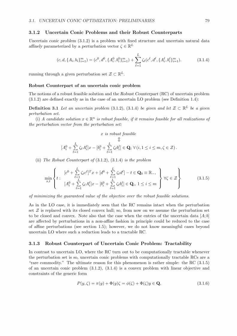
3.1.2 Uncertain Conic Problems and their Robust Counterparts
Uncertain conic problem (3.1.2) is a problem with fixed structure and uncertain natural dataaffinely parameterized by a perturbation vector ζ ∈ RL
(c, d, Ai, bimi=1) = (c0, d0, A0
i , b0i m
i=1) +L∑
`=1
ζ`(c`, d`, A`i , b
`im
i=1). (3.1.4)
running through a given perturbation set Z ⊂ RL.
Robust Counterpart of an uncertain conic problem
The notions of a robust feasible solution and the Robust Counterpart (RC) of uncertain problem(3.1.2) are defined exactly as in the case of an uncertain LO problem (see Definition 1.4):
Definition 3.1 Let an uncertain problem (3.1.2), (3.1.4) be given and let Z ⊂ RL be a givenperturbation set.
(i) A candidate solution x ∈ Rn is robust feasible, if it remains feasible for all realizations ofthe perturbation vector from the perturbation set:
x is robust feasiblem
[A0i +
L∑`=1
ζ`A`i ]x− [b0
i +L∑
`=1
ζ`b`i ] ∈ Qi ∀ (i, 1 ≤ i ≤ m, ζ ∈ Z) .
(ii) The Robust Counterpart of (3.1.2), (3.1.4) is the problem
minx,t
t :[c0 +
L∑`=1
ζ`c`]T x + [d0 +
L∑`=1
ζ`d`]− t ∈ Q0 ≡ R−,
[A0i +
L∑`=1
ζ`A`i ]x− [b0
i +L∑
`=1
ζ`b`i ] ∈ Qi, 1 ≤ i ≤ m
∀ζ ∈ Z
(3.1.5)
of minimizing the guaranteed value of the objective over the robust feasible solutions.
As in the LO case, it is immediately seen that the RC remains intact when the perturbationset Z is replaced with its closed convex hull; so, from now on we assume the perturbation setto be closed and convex. Note also that the case when the entries of the uncertain data [A; b]are affected by perturbations in a non-affine fashion in principle could be reduced to the caseof affine perturbations (see section 1.5); however, we do not know meaningful cases beyonduncertain LO where such a reduction leads to a tractable RC.
3.1.3 Robust Counterpart of Uncertain Conic Problem: Tractability
In contrast to uncertain LO, where the RC turn out to be computationally tractable wheneverthe perturbation set is so, uncertain conic problems with computationally tractable RCs are a“rare commodity.” The ultimate reason for this phenomenon is rather simple: the RC (3.1.5)of an uncertain conic problem (3.1.2), (3.1.4) is a convex problem with linear objective andconstraints of the generic form
P (y, ζ) = π(y) + Φ(y)ζ = φ(ζ) + Φ(ζ)y ∈ Q, (3.1.6)

80 LECTURE 3: ROBUST CONIC OPTIMIZATION
where π(y), Φ(y) are affine in the vector y of the decision variables, φ(ζ),Φ(ζ) are affine inthe perturbation vector ζ, and Q is a “simple” closed convex set. For such a problem, itscomputational tractability is, essentially, equivalent to the possibility to check efficiently whethera given candidate solution y is or is not feasible. The latter question, in turn, is whether theimage of the perturbation set Z under an affine mapping ζ 7→ π(y)+Φ(y)ζ is or is not containedin a given convex set Q. This question is easy when Q is a polyhedral set given by an explicitlist of scalar linear inequalities aT
i u ≤ bi, i = 1, ..., I (in particular, when Q is a nonpositive ray,that is what we deal with in LO), in which case the required verification consists in checkingwhether the maxima of I affine functions aT
i (π(y) + Φ(y)ζ) − bi of ζ over ζ ∈ Z are or arenot nonnegative. Since the maximization of an affine (and thus concave!) function over acomputationally tractable convex set Z is easy, so is the required verification. When Q is givenby nonlinear convex inequalities ai(u) ≤ 0, i = 1, ..., I, the verification in question requireschecking whether the maxima of convex functions ai(π(y) + Φ(y)ζ) over ζ ∈ Z are or are notnonpositive. A problem of maximizing a convex function f(ζ) over a convex set Z can becomputationally intractable already in the case of Z as simple as the unit box and f as simpleas a convex quadratic form ζT Qζ. Indeed, it is known that the problem
maxζ
ζT Bζ : ‖ζ‖∞ ≤ 1
with positive semidefinite matrix B is NP-hard; in fact, it is already NP-hard to approximatethe optimal value in this problem within a relative accuracy of 4%, even when probabilisticalgorithms are allowed [55]. This example immediately implies that the RC of a generic un-certain conic quadratic problem with a perturbation set as simple as a box is computationallyintractable.
Indeed, consider a simple-looking uncertain conic quadratic inequality
‖0 · y + Qζ‖2 ≤ 1
(Q is a given square matrix) along with its RC, the perturbation set being the unit box:
‖0 · y + Qζ‖2 ≤ 1 ∀(ζ : ‖ζ‖∞ ≤ 1). (RC)
The feasible set of the RC is either the entire space of y-variables, or is empty, which dependson whether or not one has
max‖ζ‖∞≤1
ζT Bζ ≤ 1. [B = QT Q]
Varying Q, we can get, as B, an arbitrary positive semidefinite matrix of a given size. Now,assuming that we can process (RC) efficiently, we can check efficiently whether the feasibleset of (RC) is or is not empty, that is, we can compare efficiently the maximum of a positivesemidefinite quadratic form over the unit box with the value 1. If we can do it, we cancompute the maximum of a general-type positive semidefinite quadratic form ζT Bζ over theunit box within relative accuracy ε in time polynomial in the dimension of ζ and ln(1/ε) (bycomparing max‖ζ‖∞≤1 λζT Bζ with 1 and applying bisection in λ > 0). Thus, the NP-hardproblem of computing max‖ζ‖∞≤1 ζT Bζ, B Â 0, within relative accuracy ε = 0.04 reducesto checking feasibility of the RC of a CQI with a box perturbation set, meaning that it isNP-hard to process the RC in question.
The unpleasant phenomenon we have just outlined leaves us with only two options:A. To identify meaningful particular cases where the RC of an uncertain conic problem is
computationally tractable; and

3.1. UNCERTAIN CONIC OPTIMIZATION: PRELIMINARIES 81
B. To develop tractable approximations of the RC in the remaining cases.Note that the RC, same as in the LO case, is a “constraint-wise” construction, so that
investigating tractability of the RC of an uncertain conic problem reduces to the same questionfor the RCs of the conic constraints constituting the problem. Due to this observation, fromnow on we focus on tractability of the RC
∀(ζ ∈ Z) : A(ζ)x + b(ζ) ∈ Q
of a single uncertain conic inequality.
3.1.4 Safe Tractable Approximations of RCs of Uncertain Conic Inequalities
In sections 3.2, 3.4 we will present a number of special cases where the RC of an uncertainCQI/LMI is computationally tractable; these cases have to do with rather specific perturbationsets. The question is, what to do when the RC is not computationally tractable. A naturalcourse of action in this case is to look for a safe tractable approximation of the RC, defined asfollows:
Definition 3.2 Consider the RC
A(ζ)x + b(ζ)︸ ︷︷ ︸≡α(x)ζ+β(x)
∈ Q ∀ζ ∈ Z (3.1.7)
of an uncertain constraintA(ζ)x + b(ζ) ∈ Q. (3.1.8)
(A(ζ) ∈ Rk×n, b(ζ) ∈ Rk are affine in ζ, so that α(x), β(x) are affine in the decision vector x).We say that a system S of convex constraints in variables x and, perhaps, additional variablesu is a safe approximation of the RC (3.1.7), if the projection of the feasible set of S on the spaceof x variables is contained in the feasible set of the RC:
∀x : (∃u : (x, u) satisfies S) ⇒ x satisfies (3.1.7).
This approximation is called tractable, provided that S is so, (e.g., S is an explicit system ofCQIs/LMIs or, more generally, the constraints in S are efficiently computable).
The rationale behind the definition is as follows: assume we are given an uncertain conic problem(3.1.2) with vector of design variables x and a certain objective cT x (as we remember, the latterassumption is w.l.o.g.) and we have at our disposal a safe tractable approximation Si of i-thconstraint of the problem, i = 1, ..., m. Then the problem
minx,u1,...,um
cT x : (x, ui) satisfies Si, 1 ≤ i ≤ m
is a computationally tractable safe approximation of the RC, meaning that the x-component ofevery feasible solution to the approximation is feasible for the RC, and thus an optimal solutionto the approximation is a feasible suboptimal solution to the RC.
In principle, there are many ways to build a safe tractable approximation of an uncertainconic problem. For example, assuming Z bounded, which usually is the case, we could find asimplex ∆ = Convζ1, ..., ζL+1 in the space RL of perturbation vectors that is large enough tocontain the actual perturbation set Z. The RC of our uncertain problem, the perturbation set

82 LECTURE 3: ROBUST CONIC OPTIMIZATION
being ∆, is computationally tractable (see section 3.2.1) and is a safe approximation of the RCassociated with the actual perturbation set Z due to ∆ ⊃ Z. The essence of the matter is, ofcourse, how conservative an approximation is: how much it “adds” to the built-in conservatismof the worst-case-oriented RC. In order to answer the latter question, we should quantify the“conservatism” of an approximation. There is no evident way to do it. One possible way couldbe to look by how much the optimal value of the approximation is larger than the optimal valueof the true RC, but here we run into a severe difficulty. It may well happen that the feasibleset of an approximation is empty, while the true feasible set of the RC is not so. Whenever thisis the case, the optimal value of the approximation is “infinitely worse” than the true optimalvalue. It follows that comparison of optimal values makes sense only when the approximationscheme in question guarantees that the approximation inherits the feasibility properties of thetrue problem. On a closer inspection, such a requirement is, in general, not less restrictive thanthe requirement for the approximation to be precise.
The way to quantify the conservatism of an approximation to be used in this book is asfollows. Assume that 0 ∈ Z (this assumption is in full accordance with the interpretation ofvectors ζ ∈ Z as data perturbations, in which case ζ = 0 corresponds to the nominal data). Withthis assumption, we can embed our closed convex perturbation set Z into a single-parametricfamily of perturbation sets
Zρ = ρZ, 0 < ρ ≤ ∞, (3.1.9)
thus giving rise to a single-parametric family
A(ζ)x + b(ζ)︸ ︷︷ ︸≡α(x)ζ+β(x)
∈ Q ∀ζ ∈ Zρ (RCρ)
of RCs of the uncertain conic constraint (3.1.8). One can think about ρ as perturbation level;the original perturbation set Z and the associated RC (3.1.7) correspond to the perturbationlevel 1. Observe that the feasible set Xρ of (RCρ) shrinks as ρ grows. This allows us to quantifythe conservatism of a safe approximation to (RC) by “positioning” the feasible set of S withrespect to the scale of “true” feasible sets Xρ, specifically, as follows:
Definition 3.3 Assume that we are given an approximation scheme that puts into correspon-dence to (3.1.9), (RCρ) a finite system Sρ of efficiently computable convex constraints on variablesx and, perhaps, additional variables u, depending on ρ > 0 as on a parameter, in such a waythat for every ρ the system Sρ is a safe tractable approximation of (RCρ), and let Xρ be theprojection of the feasible set of Sρ onto the space of x variables.
We say that the conservatism (or “tightness factor”) of the approximation scheme in questiondoes not exceed ϑ ≥ 1 if, for every ρ > 0, we have
Xϑρ ⊂ Xρ ⊂ Xρ.
Note that the fact that Sρ is a safe approximation of (RCρ) tight within factor ϑ is equivalentto the following pair of statements:
1. [safety] Whenever a vector x and ρ > 0 are such that x can be extended to a feasiblesolution of Sρ, x is feasible for (RCρ);
2. [tightness] Whenever a vector x and ρ > 0 are such that x cannot be extended to a feasiblesolution of Sρ, x is not feasible for (RCϑρ).

3.2. UNCERTAIN CONIC QUADRATIC PROBLEMS WITH TRACTABLE RCS 83
Clearly, a tightness factor equal to 1 means that the approximation is precise: Xρ = Xρ forall ρ. In many applications, especially in those where the level of perturbations is known only“up to an order of magnitude,” a safe approximation of the RC with a moderate tightness factoris almost as useful, from a practical viewpoint, as the RC itself.
An important observation is that with a bounded perturbation set Z = Z1 ⊂ RL that is sym-metric w.r.t. the origin, we can always point out a safe computationally tractable approximationscheme for (3.1.9), (RCρ) with tightness factor ≤ L.Indeed, w.l.o.g. we may assume that intZ 6= ∅, so that Z is a closed and bounded convex set symmetricw.r.t. the origin. It is known that for such a set, there always exist two similar ellipsoids, centeredat the origin, with the similarity ratio at most
√L, such that the smaller ellipsoid is contained in Z,
and the larger one contains Z. In particular, one can choose, as the smaller ellipsoid, the largest volumeellipsoid contained in Z; alternatively, one can choose, as the larger ellipsoid, the smallest volume ellipsoidcontaining Z. Choosing coordinates in which the smaller ellipsoid is the unit Euclidean ball B, weconclude that B ⊂ Z ⊂ √
LB. Now observe that B, and therefore Z, contains the convex hull Z = ζ ∈RL : ‖ζ‖1 ≤ 1 of the 2L vectors ±e`, ` = 1, ..., L, where e` are the basic orths of the axes in question.Since Z clearly contains L−1/2B, the convex hull Z of the vectors ±Le`, ` = 1, ..., L, contains Z and iscontained in LZ. Taking, as Sρ, the RC of our uncertain constraint, the perturbation set being ρZ, weclearly get an L-tight safe approximation of (3.1.9), (RCρ), and this approximation is merely the systemof constraints
A(ρLe`)x + b(ρLe`) ∈ Q, A(−ρLe`)x + b(−ρLe`) ∈ Q, ` = 1, ..., L,
that is, our approximation scheme is computationally tractable.
3.2 Uncertain Conic Quadratic Problems with Tractable RCs
In this section we focus on uncertain conic quadratic problems (that is, the sets Qi in (3.1.2)are given by explicit lists of conic quadratic inequalities) for which the RCs are computationallytractable.
3.2.1 A Generic Solvable Case: Scenario Uncertainty
We start with a simple case where the RC of an uncertain conic problem (not necessarily a conicquadratic one) is computationally tractable — the case of scenario uncertainty.
Definition 3.4 We say that a perturbation set Z is scenario generated, if Z is given as theconvex hull of a given finite set of scenarios ζ(ν):
Z = Convζ(1), ..., ζ(N). (3.2.1)
Theorem 3.1 The RC (3.1.5) of uncertain problem (3.1.2), (3.1.4) with scenario perturbationset (3.2.1) is equivalent to the explicit conic problem
minx,t
t :
[c0 +L∑
`=1
ζ(ν)` c`]T x + [d0 +
L∑`=1
ζ(ν)` d`]− t ≤ 0
[A0i +
L∑`=1
ζ(ν)` A`
i ]T x− [b0 +
L∑`=1
ζ(ν)` b`] ∈ Qi,
1 ≤ i ≤ m
, 1 ≤ ν ≤ N
(3.2.2)
with a structure similar to the one of the instances of the original uncertain problem.

84 LECTURE 3: ROBUST CONIC OPTIMIZATION
Proof. This is evident due to the convexity of Qi and the affinity of the left hand sides of theconstraints in (3.1.5) in ζ. ¤
The situation considered in Theorem 3.1 is “symmetric” to the one considered in lecture 1,where we spoke about problems (3.1.2) with the simplest possible sets Qi — just nonnegativerays, and the RC turns out to be computationally tractable whenever the perturbation set isso. Theorem 3.1 deals with another extreme case of the tradeoff between the geometry of theright hand side sets Qi and that of the perturbation set. Here the latter is as simple as it couldbe — just the convex hull of an explicitly listed finite set, which makes the RC computationallytractable for rather general (just computationally tractable) sets Qi. Unfortunately, the secondextreme is not too interesting: in the large scale case, a “scenario approximation” of a reasonablequality for typical perturbation sets, like boxes, requires an astronomically large number ofscenarios, thus preventing listing them explicitly and making problem (3.2.2) computationallyintractable. This is in sharp contrast with the first extreme, where the simple sets were Qi —Linear Optimization is definitely interesting and has a lot of applications.
In what follows, we consider a number of less trivial cases where the RC of an uncertain conicquadratic problem is computationally tractable. As always with RC, which is a constraint-wiseconstruction, we may focus on computational tractability of the RC of a single uncertain CQI
‖A(ζ)y + b(ζ)︸ ︷︷ ︸≡α(y)ζ+β(y)
‖2 ≤ cT (ζ)y + d(ζ)︸ ︷︷ ︸≡σT (y)ζ+δ(y)
, (3.2.3)
where A(ζ) ∈ Rk×n, b(ζ) ∈ Rk, c(ζ) ∈ Rn, d(ζ) ∈ R are affine in ζ, so that α(y), β(y), σ(y), δ(y)are affine in the decision vector y.
3.2.2 Solvable Case I: Simple Interval Uncertainty
Consider uncertain conic quadratic constraint (3.2.3) and assume that:
1. The uncertainty is side-wise: the perturbation set Z = Z left ×Zright is the direct productof two sets (so that the perturbation vector ζ ∈ Z is split into blocks η ∈ Z left andχ ∈ Zright), with the left hand side data A(ζ), b(ζ) depending solely on η and the righthand side data c(ζ), d(ζ) depending solely on χ, so that (3.2.3) reads
‖A(η)y + b(η)︸ ︷︷ ︸≡α(y)η+β(y)
‖2 ≤ cT (χ)y + d(χ)︸ ︷︷ ︸≡σT (y)χ+δ(y)
, (3.2.4)
and the RC of this uncertain constraint reads
‖A(η)y + b(η)‖2 ≤ cT (χ)y + d(χ) ∀(η ∈ Z left, χ ∈ Zright); (3.2.5)
2. The right hand side perturbation set is as described in Theorem 1.1, that is,
Zright = χ : ∃u : Pχ + Qu + p ∈ K ,
where either K is a closed convex pointed cone, and the representation is strictly feasible,or K is a polyhedral cone given by an explicit finite list of linear inequalities;

3.2. UNCERTAIN CONIC QUADRATIC PROBLEMS WITH TRACTABLE RCS 85
3. The left hand side uncertainty is a simple interval one:
Z left =η = [δA, δb] : |(δA)ij | ≤ δij , 1 ≤ i ≤ k, 1 ≤ j ≤ n,|(δb)i| ≤ δi, 1 ≤ i ≤ k
,
[A(ζ), b(ζ)] = [An, bn] + [δA, δb].
In other words, every entry in the left hand side data [A, b] of (3.2.3), independently of allother entries, runs through a given segment centered at the nominal value of the entry.
Proposition 3.1 Under assumptions 1 – 3 on the perturbation set Z, the RC of the uncertainCQI (3.2.3) is equivalent to the following explicit system of conic quadratic and linear constraintsin variables y, z, τ, v:
(a)τ + pT v ≤ δ(y), P T v = σ(y),QT v = 0, v ∈ K∗
(b)zi ≥ |(Any + bn)i|+ δi +
n∑j=1
|δijyj |, i = 1, ..., k
‖z‖2 ≤ τ
(3.2.6)
where K∗ is the cone dual to K.
Proof. Due to the side-wise structure of the uncertainty, a given y is robust feasible if and onlyif there exists τ such that
(a) τ ≤ minχ∈Zright
σT (y)χ + δ(y)
= minχ,u
σT (y)χ : Pχ + Qu + p ∈ K
+ δ(y),
(b) τ ≥ maxη∈Zleft
‖A(η)y + b(η)‖2
= maxδA,δb
‖[Any + bn] + [δAy + δb]‖2 : |δA|ij ≤ δij , |δbi| ≤ δi .
By Conic Duality, a given τ satisfies (a) if and only if τ can be extended, by properly chosen v,to a solution of (3.2.6.a); by evident reasons, τ satisfies (b) if and only if there exists z satisfying(3.2.6.b). ¤
3.2.3 Solvable Case II: Unstructured Norm-Bounded Uncertainty
Consider the case where the uncertainty in (3.2.3) is still side-wise (Z = Z left×Zright) with theright hand side uncertainty set Zright as in section 3.2.2, while the left hand side uncertainty isunstructured norm-bounded, meaning that
Z left =η ∈ Rp×q : ‖η‖2,2 ≤ 1
(3.2.7)
and eitherA(η)y + b(η) = Any + bn + LT (y)ηR (3.2.8)
with L(y) affine in y and R 6= 0, or
A(η)y + b(η) = Any + bn + LT ηR(y) (3.2.9)
with R(y) affine in y and L 6= 0. Here
‖η‖2,2 = maxu‖ηu‖2 : u ∈ Rq, ‖u‖2 ≤ 1
is the usual matrix norm of a p× q matrix η (the maximal singular value),

86 LECTURE 3: ROBUST CONIC OPTIMIZATION
Example 3.1(i) Imagine that some p× q submatrix P of the left hand side data [A, b] of (3.2.4) is uncertain and
differs from its nominal value Pn by an additive perturbation ∆P = MT ∆N with ∆ having matrix normat most 1, and all entries in [A, b] outside of P are certain. Denoting by I the set of indices of the rowsin P and by J the set of indices of the columns in P , let U be the natural projector of Rn+1 on thecoordinate subspace in Rn+1 given by J , and V be the natural projector of Rk on the subspace of Rk
given by I (e.g., with I = 1, 2 and J = 1, 5, Uu = [u1; u5] ∈ R2 and V u = [u1; u2] ∈ R2). Then theoutlined perturbations of [A, b] can be represented as
[A(η), b(η)] = [An, bn] + V T MT︸ ︷︷ ︸LT
η (NU)︸ ︷︷ ︸R
, ‖η‖2,2 ≤ 1,
whence, setting Y (y) = [y; 1],
A(η)y + b(η) = [Any + bn] + LT η [RY (y)]︸ ︷︷ ︸R(y)
,
and we are in the situation (3.2.7), (3.2.9).(ii) [Simple ellipsoidal uncertainty] Assume that the left hand side perturbation set Z left is a p-
dimensional ellipsoid; w.l.o.g. we may assume that this ellipsoid is just the unit Euclidean ball B = η ∈Rp : ‖η‖2 ≤ 1. Note that for vectors η ∈ Rp = Rp×1 their usual Euclidean norm ‖η‖2 and their matrixnorm ‖η‖2,2 are the same. We now have
A(η)y + b(η) = [A0y + b0] +p∑
`=1
η`[A`y + b`] = [Any + bn] + LT (y)ηR,
where An = A0, bn = b0, R = 1 and L(y) is the matrix with the rows [A`y + b`]T , ` = 1, ..., p. Thus, weare in the situation (3.2.7), (3.2.8).
Theorem 3.2 The RC of the uncertain CQI (3.2.4) with unstructured norm-bounded uncer-tainty is equivalent to the following explicit system of LMIs in variables y, τ, u, λ:(i) In the case of left hand side perturbations (3.2.7), (3.2.8):
(a) τ + pT v ≤ δ(y), P T v = σ(y), QT v = 0, v ∈ K∗
(b)
τIk LT (y) Any + bn
L(y) λIp
[Any + bn]T τ − λRT R
º 0.
(3.2.10)
(ii) In the case of left hand side perturbations (3.2.7), (3.2.9):
(a) τ + pT v ≤ δ(y), P T v = σ(y), QT v = 0, v ∈ K∗
(b)
τIk − λLT L Any + bn
λIq R(y)[Any + bn]T RT (y) τ
º 0.
(3.2.11)
Here K∗ is the cone dual to K.

3.2. UNCERTAIN CONIC QUADRATIC PROBLEMS WITH TRACTABLE RCS 87
Proof. Same as in the proof of Proposition 3.1, y is robust feasible for (3.2.4) if and only ifthere exists τ such that
(a) τ ≤ minχ∈Zright
σT (y)χ + δ(y)
= minχ,u
σT (y)χ : Pχ + Qu + p ∈ K
,
(b) τ ≥ maxη∈Zleft
‖A(η)y + b(η)‖2,
(3.2.12)
and a given τ satisfies (a) if and only if it can be extended, by a properly chosen v, to a solutionof (3.2.10.a)⇔(3.2.11.a). It remains to understand when τ satisfies (b). This requires two basicfacts.
Lemma 3.1 [Semidefinite representation of the Lorentz cone] A vector [y; t] ∈ Rk × R belongsto the Lorentz cone Lk+1 = [y; t] ∈ Rk+1 : t ≥ ‖y‖2 if and only if the “arrow matrix”
Arrow(y, t) =[
t yT
y tIk
]
is positive semidefinite.
Proof of Lemma 3.1: We use the following fundamental fact:
Lemma 3.2 [Schur Complement Lemma] A symmetric block matrix
A =[
P QT
Q R
]
with R Â 0 is positive (semi)definite if and only if the matrix
P −QT R−1Q
is positive (semi)definite.
Schur Complement Lemma ⇒ Lemma 3.1: When t = 0, we have [y; t] ∈ Lk+1 iff y = 0, andArrow(y, t) º 0 iff y = 0, as claimed in Lemma 3.1. Now let t > 0. Then the matrix tIk ispositive definite, so that by the Schur Complement Lemma we have Arrow(y, t) º 0 if and onlyif t ≥ t−1yT y, or, which is the same, iff [y; t] ∈ Lk+1. When t < 0, we have [y; t] 6∈ Lk+1 andArrow(y, t) 6º 0. ¤Proof of the Schur Complement Lemma: Matrix A = AT is º 0 iff uT Pu+2uT QT v + vT Rv ≥ 0for all u, v, or, which is the same, iff
∀u : 0 ≤ minv
uT Pu + 2uT QT v + vT Rv
= uT Pu− uT QT R−1Qu
(indeed, since R Â 0, the minimum in v in the last expression is achieved when v = R−1Qu).The concluding relation ∀u : uT [P −QT R−1Q]u ≥ 0 is valid iff P −QT R−1Q º 0. Thus, A º 0iff P −QT R−1Q º 0. The same reasoning implies that A Â 0 iff P −QT R−1Q Â 0. ¤
We further need the following fundamental result:

88 LECTURE 3: ROBUST CONIC OPTIMIZATION
Lemma 3.3 [S-Lemma](i) [homogeneous version] Let A,B be symmetric matrices of the same size such that xT Ax >
0 for some x. Then the implication
xT Ax ≥ 0 ⇒ xT Bx ≥ 0
holds true if and only if
∃λ ≥ 0 : B º λA.
(ii) [inhomogeneous version] Let A,B be symmetric matrices of the same size, and let thequadratic form xT Ax + 2aT x + α be strictly positive at some point. Then the implication
xT Ax + 2aT x + α ≥ 0 ⇒ xT Bx + 2bT x + β ≥ 0
holds true if and only if
∃λ ≥ 0 :[
B − λA bT − λaT
b− λa β − λα
]º 0.
For proof of this fundamental Lemma, see, e.g., [9, section 4.3.5].Coming back to the proof of Theorem 3.2, we can now understand when a given pair τ, y
satisfies (3.2.12.b). Let us start with the case (3.2.8). We have
(y, τ) satisfies (3.2.12.b)
⇔ [
y︷ ︸︸ ︷[Any + bn]+LT (y)ηR; τ ] ∈ Lk+1 ∀(η : ‖η‖2,2 ≤ 1)
[by (3.2.8)]
⇔[
τ yT + RT ηT L(y)y + LT (y)ηR τIk
]º 0 ∀(η : ‖η‖2,2 ≤ 1)
[by Lemma 3.1]
⇔ τs2 + 2srT [y + LT (y)ηR] + τrT r ≥ 0 ∀[s; r] ∀(η : ‖η‖2,2 ≤ 1)
⇔ τs2 + 2syT r + 2 minη:‖η‖2,2≤1
[s(ηT L(y)r)T R
]+ τrT r ≥ 0 ∀[s; r]
⇔ τs2 + 2syT r − 2‖L(y)r‖2‖sR‖2 + τrT r ≥ 0 ∀[s; r]
⇔ τrT r + 2(L(y)r)T ξ + 2srT y + τs2 ≥ 0 ∀(s, r, ξ : ξT ξ ≤ s2RT R)
⇔ ∃λ ≥ 0 :
τIk LT (y) y
L(y) λIp
yT τ − λRT R
º 0
[by the homogeneous S-Lemma; note that R 6= 0].
The requirement λ ≥ 0 in the latter relation is implied by the LMI in the relation and is thereforeredundant. Thus, in the case of (3.2.8) relation (3.2.12.b) is equivalent to the possibility to extend(y, τ) to a solution of (3.2.10.b).
3.2. UNCERTAIN CONIC QUADRATIC PROBLEMS WITH TRACTABLE RCS 89
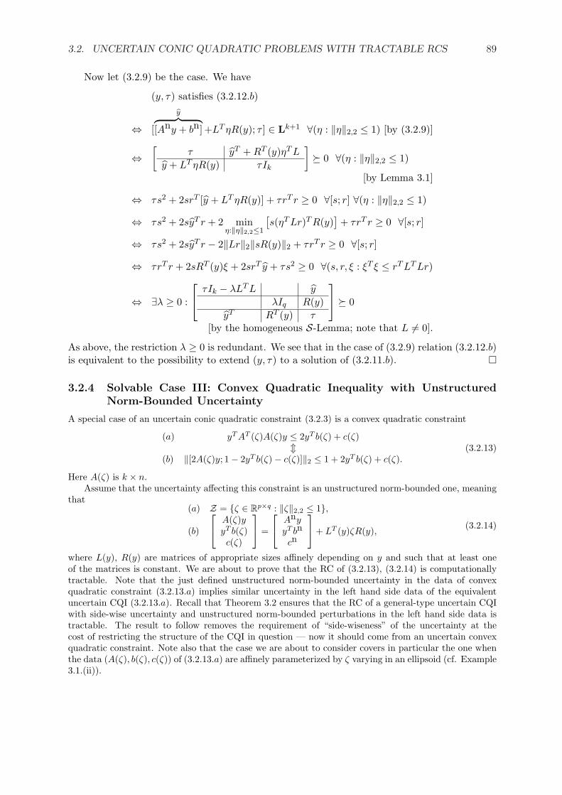
Now let (3.2.9) be the case. We have
(y, τ) satisfies (3.2.12.b)
⇔ [
y︷ ︸︸ ︷[Any + bn]+LT ηR(y); τ ] ∈ Lk+1 ∀(η : ‖η‖2,2 ≤ 1) [by (3.2.9)]
⇔[
τ yT + RT (y)ηT L
y + LT ηR(y) τIk
]º 0 ∀(η : ‖η‖2,2 ≤ 1)
[by Lemma 3.1]
⇔ τs2 + 2srT [y + LT ηR(y)] + τrT r ≥ 0 ∀[s; r] ∀(η : ‖η‖2,2 ≤ 1)
⇔ τs2 + 2syT r + 2 minη:‖η‖2,2≤1
[s(ηT Lr)T R(y)
]+ τrT r ≥ 0 ∀[s; r]
⇔ τs2 + 2syT r − 2‖Lr‖2‖sR(y)‖2 + τrT r ≥ 0 ∀[s; r]
⇔ τrT r + 2sRT (y)ξ + 2srT y + τs2 ≥ 0 ∀(s, r, ξ : ξT ξ ≤ rT LT Lr)
⇔ ∃λ ≥ 0 :
τIk − λLT L y
λIq R(y)yT RT (y) τ
º 0
[by the homogeneous S-Lemma; note that L 6= 0].
As above, the restriction λ ≥ 0 is redundant. We see that in the case of (3.2.9) relation (3.2.12.b)is equivalent to the possibility to extend (y, τ) to a solution of (3.2.11.b). ¤
3.2.4 Solvable Case III: Convex Quadratic Inequality with UnstructuredNorm-Bounded Uncertainty
A special case of an uncertain conic quadratic constraint (3.2.3) is a convex quadratic constraint
(a) yT AT (ζ)A(ζ)y ≤ 2yT b(ζ) + c(ζ)m
(b) ‖[2A(ζ)y; 1− 2yT b(ζ)− c(ζ)]‖2 ≤ 1 + 2yT b(ζ) + c(ζ).(3.2.13)
Here A(ζ) is k × n.Assume that the uncertainty affecting this constraint is an unstructured norm-bounded one, meaning
that(a) Z = ζ ∈ Rp×q : ‖ζ‖2,2 ≤ 1,
(b)
A(ζ)yyT b(ζ)c(ζ)
=
AnyyT bn
cn
+ LT (y)ζR(y), (3.2.14)
where L(y), R(y) are matrices of appropriate sizes affinely depending on y and such that at least oneof the matrices is constant. We are about to prove that the RC of (3.2.13), (3.2.14) is computationallytractable. Note that the just defined unstructured norm-bounded uncertainty in the data of convexquadratic constraint (3.2.13.a) implies similar uncertainty in the left hand side data of the equivalentuncertain CQI (3.2.13.a). Recall that Theorem 3.2 ensures that the RC of a general-type uncertain CQIwith side-wise uncertainty and unstructured norm-bounded perturbations in the left hand side data istractable. The result to follow removes the requirement of “side-wiseness” of the uncertainty at thecost of restricting the structure of the CQI in question — now it should come from an uncertain convexquadratic constraint. Note also that the case we are about to consider covers in particular the one whenthe data (A(ζ), b(ζ), c(ζ)) of (3.2.13.a) are affinely parameterized by ζ varying in an ellipsoid (cf. Example3.1.(ii)).

90 LECTURE 3: ROBUST CONIC OPTIMIZATION
Proposition 3.2 Let us set L(y) = [LA(y), Lb(y), Lc(y)], where Lb(y), Lc(y) are the last two columnsin L(y), and let
LT (y) =[LT
b (y) + 12LT
c (y); LTA(y)
], R(y) = [R(y), 0q×k],
A(y) =[
2yT bn + cn [Any]T
Any Ik
],
(3.2.15)
so that A(y), L(y) and R(y) are affine in y and at least one of the latter two matrices is constant.
The RC of (3.2.13), (3.2.14) is equivalent to the explicit LMI S in variables y, λ as follows:
(i) In the case when L(y) is independent of y and is nonzero, S is
[A(y)− λLT L RT (y)
R(y) λIq
]º 0; (3.2.16)
(ii) In the case when R(Y ) is independent of y and is nonzero, S is
[A(y)− λRT R LT (y)
L(y) λIp
]º 0; (3.2.17)
(iii) In all remaining cases (that is, when either L(y) ≡ 0, or R(y) ≡ 0, or both), S is
A(y) º 0. (3.2.18)
Proof. We have
yT AT (ζ)A(ζ)y ≤ 2yT b(ζ) + c(ζ) ∀ζ ∈ Z
⇔[
2yT b(ζ) + c(ζ) [A(ζ)y]T
A[ζ]y Ik
]º 0 ∀ζ ∈ Z
[Schur Complement Lemma]
⇔
A(y)︷ ︸︸ ︷[2yT bn + cn [Any]T
Any I
]
+
B(y,ζ)︷ ︸︸ ︷[2LT
b (y)ζR(y) + LTc (y)ζR(y) RT (y)ζT LA(y)
LTA(y)ζR(y)
]º 0 ∀(ζ : ‖ζ‖2,2 ≤ 1)
[by (3.2.14)]
⇔ A(y) + LT (y)ζR(y) + RT (y)ζT L(y) º 0 ∀(ζ : ‖ζ‖2,2 ≤ 1) [by (3.2.15)].
Now the reasoning can be completed exactly as in the proof of Theorem 3.2. Consider, e.g., the case of
3.2. UNCERTAIN CONIC QUADRATIC PROBLEMS WITH TRACTABLE RCS 91
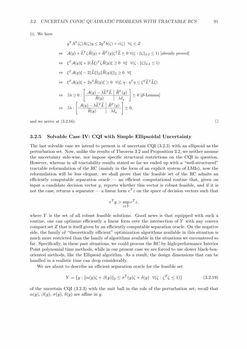
(i). We have
yT AT (ζ)A(ζ)y ≤ 2yT b(ζ) + c(ζ) ∀ζ ∈ Z
⇔ A(y) + LT ζR(y) + RT (y)ζT L º 0 ∀(ζ : ‖ζ‖2,2 ≤ 1) [already proved]
⇔ ξTA(y)ξ + 2(Lξ)T ζR(y)ξ ≥ 0 ∀ξ ∀(ζ : ‖ζ‖2,2 ≤ 1)
⇔ ξTA(y)ξ − 2‖Lξ‖2‖R(y)ξ‖2 ≥ 0 ∀ξ
⇔ ξTA(y)ξ + 2ηT R(y)ξ ≥ 0 ∀(ξ, η : ηT η ≤ ξT LT Lξ)
⇔ ∃λ ≥ 0 :
[A(y)− λLT L RT (y)
R(y) λIq
]º 0 [S-Lemma]
⇔ ∃λ :
[A(y)− λLT L RT (y)
R(y) λIq
]º 0,
and we arrive at (3.2.16). ¤
3.2.5 Solvable Case IV: CQI with Simple Ellipsoidal Uncertainty
The last solvable case we intend to present is of uncertain CQI (3.2.3) with an ellipsoid as theperturbation set. Now, unlike the results of Theorem 3.2 and Proposition 3.2, we neither assumethe uncertainty side-wise, nor impose specific structural restrictions on the CQI in question.However, whereas in all tractability results stated so far we ended up with a “well-structured”tractable reformulation of the RC (mainly in the form of an explicit system of LMIs), now thereformulation will be less elegant: we shall prove that the feasible set of the RC admits anefficiently computable separation oracle — an efficient computational routine that, given oninput a candidate decision vector y, reports whether this vector is robust feasible, and if it isnot the case, returns a separator — a linear form eT z on the space of decision vectors such that
eT y > supz∈Y
eT z,
where Y is the set of all robust feasible solutions. Good news is that equipped with such aroutine, one can optimize efficiently a linear form over the intersection of Y with any convexcompact set Z that is itself given by an efficiently computable separation oracle. On the negativeside, the family of “theoretically efficient” optimization algorithms available in this situation ismuch more restricted than the family of algorithms available in the situations we encountered sofar. Specifically, in these past situations, we could process the RC by high-performance InteriorPoint polynomial time methods, while in our present case we are forced to use slower black-box-oriented methods, like the Ellipsoid algorithm. As a result, the design dimensions that can behandled in a realistic time can drop considerably.
We are about to describe an efficient separation oracle for the feasible set
Y = y : ‖α(y)ζ + β(y)‖2 ≤ σT (y)ζ + δ(y) ∀(ζ : ζT ζ ≤ 1) (3.2.19)
of the uncertain CQI (3.2.3) with the unit ball in the role of the perturbation set; recall thatα(y), β(y), σ(y), δ(y) are affine in y.
92 LECTURE 3: ROBUST CONIC OPTIMIZATION
Observe that y ∈ Y if and only if the following two conditions hold true:
0 ≤ σT (y)ζ + δ(y) ∀(ζ : ‖ζ‖2 ≤ 1)⇔ ‖σ(y)‖2 ≤ δ(y) (a)
(σT (y)ζ + δ(y))2 − [α(y)ζ + β(y)]T [α(y)ζ + β(y)] ≥ 0∀(ζ : ζT ζ ≤ 1)
⇔ ∃λ ≥ 0 :
Ay(λ) ≡
λIL + σ(y)σT (y)−αT (y)α(y)
δ(y)σT (y)−βT (y)α(y)
δ(y)σ(y)−αT (y)β(y)
δ2(y)− βT (y)β(y)−λ
º 0 (b)
(3.2.20)
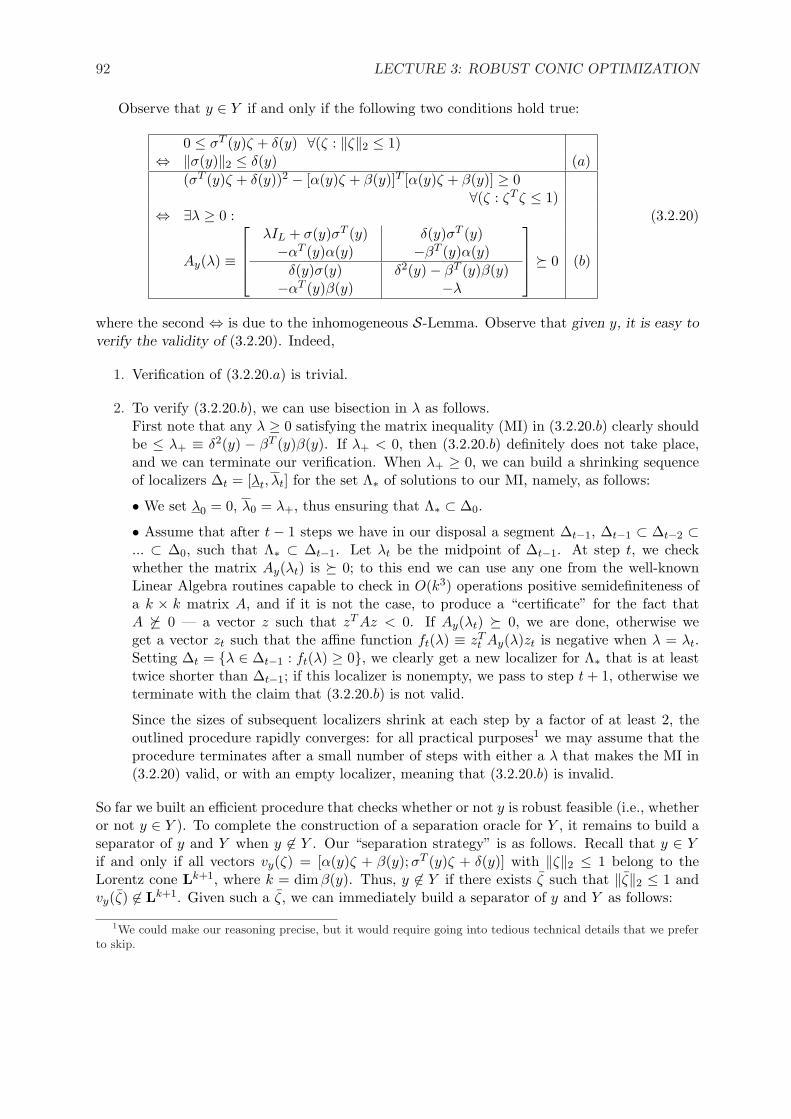
where the second ⇔ is due to the inhomogeneous S-Lemma. Observe that given y, it is easy toverify the validity of (3.2.20). Indeed,
1. Verification of (3.2.20.a) is trivial.
2. To verify (3.2.20.b), we can use bisection in λ as follows.First note that any λ ≥ 0 satisfying the matrix inequality (MI) in (3.2.20.b) clearly shouldbe ≤ λ+ ≡ δ2(y) − βT (y)β(y). If λ+ < 0, then (3.2.20.b) definitely does not take place,and we can terminate our verification. When λ+ ≥ 0, we can build a shrinking sequenceof localizers ∆t = [λt, λt] for the set Λ∗ of solutions to our MI, namely, as follows:
• We set λ0 = 0, λ0 = λ+, thus ensuring that Λ∗ ⊂ ∆0.
• Assume that after t − 1 steps we have in our disposal a segment ∆t−1, ∆t−1 ⊂ ∆t−2 ⊂... ⊂ ∆0, such that Λ∗ ⊂ ∆t−1. Let λt be the midpoint of ∆t−1. At step t, we checkwhether the matrix Ay(λt) is º 0; to this end we can use any one from the well-knownLinear Algebra routines capable to check in O(k3) operations positive semidefiniteness ofa k × k matrix A, and if it is not the case, to produce a “certificate” for the fact thatA 6º 0 — a vector z such that zT Az < 0. If Ay(λt) º 0, we are done, otherwise weget a vector zt such that the affine function ft(λ) ≡ zT
t Ay(λ)zt is negative when λ = λt.Setting ∆t = λ ∈ ∆t−1 : ft(λ) ≥ 0, we clearly get a new localizer for Λ∗ that is at leasttwice shorter than ∆t−1; if this localizer is nonempty, we pass to step t + 1, otherwise weterminate with the claim that (3.2.20.b) is not valid.
Since the sizes of subsequent localizers shrink at each step by a factor of at least 2, theoutlined procedure rapidly converges: for all practical purposes1 we may assume that theprocedure terminates after a small number of steps with either a λ that makes the MI in(3.2.20) valid, or with an empty localizer, meaning that (3.2.20.b) is invalid.
So far we built an efficient procedure that checks whether or not y is robust feasible (i.e., whetheror not y ∈ Y ). To complete the construction of a separation oracle for Y , it remains to build aseparator of y and Y when y 6∈ Y . Our “separation strategy” is as follows. Recall that y ∈ Yif and only if all vectors vy(ζ) = [α(y)ζ + β(y);σT (y)ζ + δ(y)] with ‖ζ‖2 ≤ 1 belong to theLorentz cone Lk+1, where k = dim β(y). Thus, y 6∈ Y if there exists ζ such that ‖ζ‖2 ≤ 1 andvy(ζ) 6∈ Lk+1. Given such a ζ, we can immediately build a separator of y and Y as follows:
1We could make our reasoning precise, but it would require going into tedious technical details that we preferto skip.
3.2. UNCERTAIN CONIC QUADRATIC PROBLEMS WITH TRACTABLE RCS 93
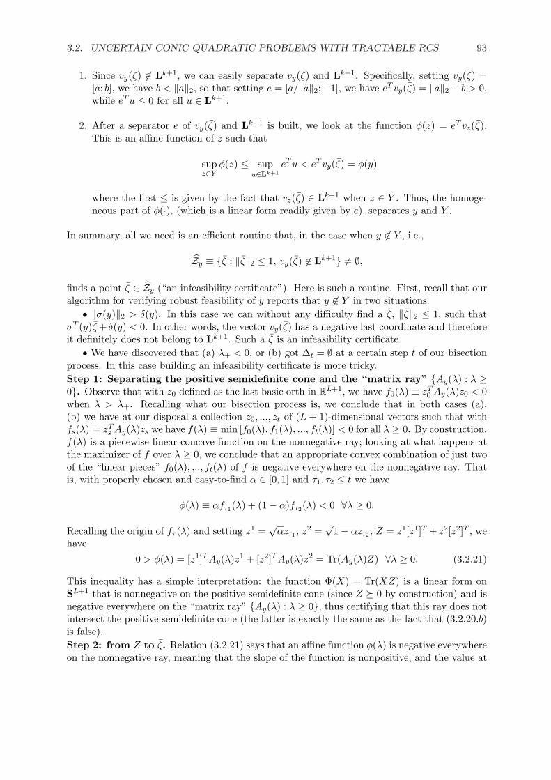
1. Since vy(ζ) 6∈ Lk+1, we can easily separate vy(ζ) and Lk+1. Specifically, setting vy(ζ) =[a; b], we have b < ‖a‖2, so that setting e = [a/‖a‖2;−1], we have eT vy(ζ) = ‖a‖2 − b > 0,while eT u ≤ 0 for all u ∈ Lk+1.
2. After a separator e of vy(ζ) and Lk+1 is built, we look at the function φ(z) = eT vz(ζ).This is an affine function of z such that
supz∈Y
φ(z) ≤ supu∈Lk+1
eT u < eT vy(ζ) = φ(y)
where the first ≤ is given by the fact that vz(ζ) ∈ Lk+1 when z ∈ Y . Thus, the homoge-neous part of φ(·), (which is a linear form readily given by e), separates y and Y .
In summary, all we need is an efficient routine that, in the case when y 6∈ Y , i.e.,
Zy ≡ ζ : ‖ζ‖2 ≤ 1, vy(ζ) 6∈ Lk+1 6= ∅,
finds a point ζ ∈ Zy (“an infeasibility certificate”). Here is such a routine. First, recall that ouralgorithm for verifying robust feasibility of y reports that y 6∈ Y in two situations:
• ‖σ(y)‖2 > δ(y). In this case we can without any difficulty find a ζ, ‖ζ‖2 ≤ 1, such thatσT (y)ζ + δ(y) < 0. In other words, the vector vy(ζ) has a negative last coordinate and thereforeit definitely does not belong to Lk+1. Such a ζ is an infeasibility certificate.
• We have discovered that (a) λ+ < 0, or (b) got ∆t = ∅ at a certain step t of our bisectionprocess. In this case building an infeasibility certificate is more tricky.Step 1: Separating the positive semidefinite cone and the “matrix ray” Ay(λ) : λ ≥0. Observe that with z0 defined as the last basic orth in RL+1, we have f0(λ) ≡ zT
0 Ay(λ)z0 < 0when λ > λ+. Recalling what our bisection process is, we conclude that in both cases (a),(b) we have at our disposal a collection z0, ..., zt of (L + 1)-dimensional vectors such that withfs(λ) = zT
s Ay(λ)zs we have f(λ) ≡ min [f0(λ), f1(λ), ..., ft(λ)] < 0 for all λ ≥ 0. By construction,f(λ) is a piecewise linear concave function on the nonnegative ray; looking at what happens atthe maximizer of f over λ ≥ 0, we conclude that an appropriate convex combination of just twoof the “linear pieces” f0(λ), ..., ft(λ) of f is negative everywhere on the nonnegative ray. Thatis, with properly chosen and easy-to-find α ∈ [0, 1] and τ1, τ2 ≤ t we have
φ(λ) ≡ αfτ1(λ) + (1− α)fτ2(λ) < 0 ∀λ ≥ 0.
Recalling the origin of fτ (λ) and setting z1 =√
αzτ1 , z2 =√
1− αzτ2 , Z = z1[z1]T + z2[z2]T , wehave
0 > φ(λ) = [z1]T Ay(λ)z1 + [z2]T Ay(λ)z2 = Tr(Ay(λ)Z) ∀λ ≥ 0. (3.2.21)
This inequality has a simple interpretation: the function Φ(X) = Tr(XZ) is a linear form onSL+1 that is nonnegative on the positive semidefinite cone (since Z º 0 by construction) and isnegative everywhere on the “matrix ray” Ay(λ) : λ ≥ 0, thus certifying that this ray does notintersect the positive semidefinite cone (the latter is exactly the same as the fact that (3.2.20.b)is false).Step 2: from Z to ζ. Relation (3.2.21) says that an affine function φ(λ) is negative everywhereon the nonnegative ray, meaning that the slope of the function is nonpositive, and the value at

94 LECTURE 3: ROBUST CONIC OPTIMIZATION
the origin is negative. Taking into account (3.2.20), we get
ZL+1,L+1 ≥L∑
i=1
Zii, Tr(Z
σ(y)σT (y)−αT (y)α(y)
δ(y)σT (y)−βT (y)α(y)
δ(y)σ(y)−αT (y)β(y)
δ2(y)− βT (y)β(y)
︸ ︷︷ ︸Ay(0)
) < 0. (3.2.22)
Besides this, we remember that Z is given as z1[z1]T + z2[z2]T . We claim that
(!) We can efficiently find a representation Z = eeT + ffT such that e, f ∈ LL+1.
Taking for the time being (!) for granted, let us build an infeasibility certificate. Indeed, fromthe second relation in (3.2.22) it follows that either Tr(Ay(0)eeT ) < 0, or Tr(Ay(0)ffT ) < 0, orboth. Let us check which one of these inequalities indeed holds true; w.l.o.g., let it be the firstone. From this inequality, in particular, e 6= 0, and since e ∈ LL+1, we have eL+1 > 0. Settinge = e/eL+1 = [ζ; 1], we have Tr(Ay(0)eeT ) = eT Ay(0)e < 0, that is,
δ2(y)− βT (y)β(y) + 2δ(y)σT (y)ζ − 2βT (y)α(y)ζ + ζT σ(y)σT (y)ζ
−ζT αT (y)α(y)ζ < 0,
or, which is the same,
(δ(y) + σT (y)ζ)2 < (α(y)ζ + β(y))T (α(y)ζ + β(y)).
We see that the vector vy(ζ) = [α(y)ζ + β(y);σT (y)ζ + δ(y)] does not belong to LL+1, whilee = [ζ; 1] ∈ LL+1, that is, ‖ζ‖2 ≤ 1. We have built a required infeasibility certificate.
It remains to justify (!). Replacing, if necessary, z1 with −z1 and z2 with −z2, we can assume thatZ = z1[z1]T + z2[z2]T with z1 = [p; s], z2 = [q; r], where s, r ≥ 0. It may happen that z1, z2 ∈ LL+1
— then we are done. Assume now that not both z1, z2 belong to LL+1, say, z1 6∈ LL+1, that is,
0 ≤ s < ‖p‖2. Observe that ZL+1,L+1 = s2 + r2 andL∑
i=1
Zii = pT p + qT q; therefore the first relation in
(3.2.22) implies that s2 + r2 ≥ pT p + qT q. Since 0 ≤ s < ‖p‖2 and r ≥ 0, we conclude that r > ‖q‖2.Thus, s < ‖p‖2, r > ‖q‖2, whence there exists (and can be easily found) α ∈ (0, 1) such that for thevector e =
√αz1 +
√1− αz2 = [u; t] we have eL+1 =
√e21 + ... + e2
L. Setting f = −√1− αz1 +√
αz2,we have eeT + ffT = z1[z1]T + z2[z2]T = Z. We now have
0 ≤ ZL+1,L+1 −L∑
i=1
Zii = e2L+1 + f2
L+1 −L∑
i=1
[e2i + f2
i ] = f2L+1 −
L∑
i=1
f2i ;
thus, replacing, if necessary, f with −f , we see that e, f ∈ LL+1 and Z = eeT + ffT , as required in (!).
Semidefinite Representation of the RC of an Uncertain CQI with Simple EllipsoidalUncertainty
This book was nearly finished when the topic considered in this section was significantly advancedby R. Hildebrand [56, 57] who discovered an explicit SDP representation of the cone of “Lorentz-positive” n×m matrices (real m× n matrices that map the Lorentz cone Lm into the Lorentzcone Ln). Existence of such a representation was a long-standing open question. As a byproductof answering this question, the construction of Hildebrand offers an explicit SDP reformulationof the RC of an uncertain conic quadratic inequality with ellipsoidal uncertainty.

3.2. UNCERTAIN CONIC QUADRATIC PROBLEMS WITH TRACTABLE RCS 95
The RC of an uncertain conic quadratic inequality with ellipsoidal uncertainty andLorentz-positive matrices. Consider the RC of an uncertain conic quadratic inequality withsimple ellipsoidal uncertainty; w.l.o.g., we assume that the uncertainty setZ is the unit Euclideanball in some Rm−1, so that the RC is the semi-infinite constraint of the form
B[x]ζ + b[x] ∈ Ln ∀(ζ ∈ Rm−1 : ζT ζ ≤ 1), (3.2.23)
with B[x], b[x] affinely depending on x. This constraint is clearly exactly the same as theconstraint
B[x]ξ + τb[x] ∈ Ln ∀([ξ; τ ] ∈ Lm).
We see that x is feasible for the RC in question if and only if the n×m matrix M [x] = [B[x], b[x]]affinely depending on x is Lorentz-positive, that is, maps the cone Lm into the cone Ln. It followsthat in order to get an explicit SDP representation of the RC, is suffices to know an explicitSDP representation of the set Pn,m of n×m matrices mapping Lm into Ln.SDP representation of Pn,m as discovered by R. Hildebrand (who used tools going far beyondthose used in this book) is as follows.
A. Given m,n, we define a linear mapping A 7→ W(A) from the space Rn×m of real n ×mmatrices into the space SN of symmetric N ×N matrices with N = (n− 1)(m− 1), namely, asfollows.
Let Wn[u] =
un + u1 u2 · · · un−1
u2 un − u1
.... . .
un−1 un − u1
, so that Wn is a symmetric (n − 1) ×
(n − 1) matrix depending on a vector u of n real variables. Now consider the Kronecker
product W [u, v] = Wn[u]⊗
Wm[v]. 2 W is a symmetric N ×N matrix with entries that arebilinear functions of u and v variables, so that an entry is of the form “weighted sum of pairproducts of the u and the v-variables.” Now, given an n ×m matrix A, let us replace pairproducts uivk in the representation of the entries in W [u, v] with the entries Aik of A. Asa result of this formal substitution, W will become a symmetric (n − 1) × (m − 1) matrixW(A) that depends linearly on A.
B. We define a linear subspace Lm,n in the space SN as the linear span of the Kroneckerproducts S
⊗T of all skew-symmetric real (n−1)× (n−1) matrices S and skew-symmetric real
(m−1)× (m−1) matrices T . Note that the Kronecker product of two skew-symmetric matricesis a symmetric matrix, so that the definition makes sense. Of course, we can easily build a basisin Lm,n — it is comprised of pairwise Kronecker products of the basic (n− 1)-dimensional and(m− 1)-dimensional skew-symmetric matrices.
The Hildebrand SDP representation of Pn,m is given by the following:
Theorem 3.3 [Hildebrand [57, Theorem 5.6]] Let min[m,n] ≥ 3. Then an n × m matrix Amaps Lm into Ln if and only if A can be extended to a feasible solution to the explicit system ofLMIs
W(A) + X º 0, X ∈ Lm,n
in variables A,X.2Recall that the Kronecker product A
⊗B of a p × q matrix A and an r × s matrix B is the pr × qs matrix
with rows indexed by pairs (i, k), 1 ≤ i ≤ p, 1 ≤ k ≤ r, and columns indexed by pairs (j, `), 1 ≤ j ≤ q, 1 ≤ ` ≤ s,and the ((i, k), (j, `))-entry equal to AijBk`. Equivalently, A
⊗B is a p × q block matrix with r × s blocks, the
(i, j)-th block being AijB.
96 LECTURE 3: ROBUST CONIC OPTIMIZATION
As a corollary,
When m − 1 := dim ζ ≥ 2 and n := dim b[x] ≥ 3, the explicit (n − 1)(m − 1) × (n − 1)(m − 1)LMI
W([B[x], b[x]]) + X º 0 (3.2.24)
in variables x and X ∈ Lm,n is an equivalent SDP representation of the semi-infinite conicquadratic inequality (3.2.23) with ellipsoidal uncertainty set.
The lower bounds on the dimensions of ζ and b[x] in the corollary do not restrict generality —we can always ensure their validity by adding zero columns to B[x] and/or adding zero rows to[B[x], b[x]].
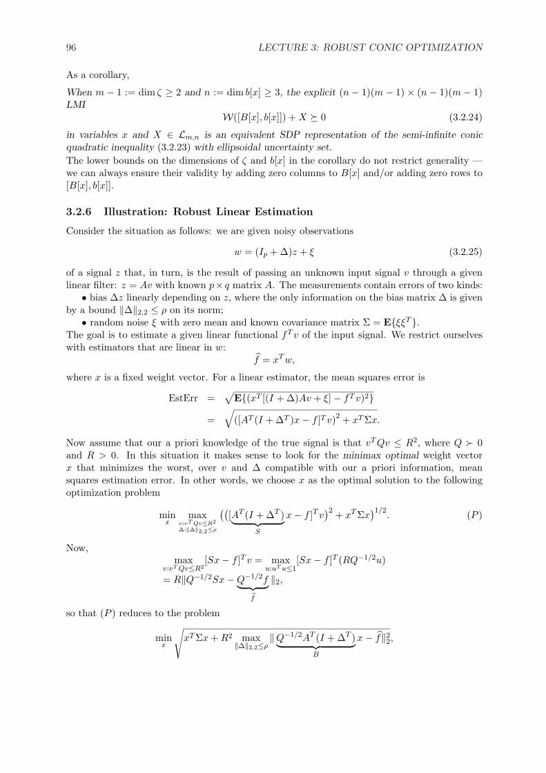
3.2.6 Illustration: Robust Linear Estimation
Consider the situation as follows: we are given noisy observations
w = (Ip + ∆)z + ξ (3.2.25)
of a signal z that, in turn, is the result of passing an unknown input signal v through a givenlinear filter: z = Av with known p× q matrix A. The measurements contain errors of two kinds:
• bias ∆z linearly depending on z, where the only information on the bias matrix ∆ is givenby a bound ‖∆‖2,2 ≤ ρ on its norm;
• random noise ξ with zero mean and known covariance matrix Σ = EξξT .The goal is to estimate a given linear functional fT v of the input signal. We restrict ourselveswith estimators that are linear in w:
f = xT w,
where x is a fixed weight vector. For a linear estimator, the mean squares error is
EstErr =√
E(xT [(I + ∆)Av + ξ]− fT v)2
=√
([AT (I + ∆T )x− f ]T v)2 + xT Σx.
Now assume that our a priori knowledge of the true signal is that vT Qv ≤ R2, where Q Â 0and R > 0. In this situation it makes sense to look for the minimax optimal weight vectorx that minimizes the worst, over v and ∆ compatible with our a priori information, meansquares estimation error. In other words, we choose x as the optimal solution to the followingoptimization problem
minx
maxv:vT Qv≤R2
∆:‖∆‖2,2≤ρ
(([AT (I + ∆T )︸ ︷︷ ︸
S
x− f ]T v)2 + xT Σx
)1/2. (P )
Now,max
v:vT Qv≤R2[Sx− f ]T v = max
u:uT u≤1[Sx− f ]T (RQ−1/2u)
= R‖Q−1/2Sx−Q−1/2f︸ ︷︷ ︸f
‖2,
so that (P ) reduces to the problem
minx
√xT Σx + R2 max
‖∆‖2,2≤ρ‖Q−1/2AT (I + ∆T )︸ ︷︷ ︸
B
x− f‖22,

3.2. UNCERTAIN CONIC QUADRATIC PROBLEMS WITH TRACTABLE RCS 97
which is exactly the RC of the uncertain conic quadratic program
minx,t,r,s
t :
√r2 + s2 ≤ t, ‖Σ1/2x‖2 ≤ r,
‖Bx− f‖2 ≤ R−1s
, (3.2.26)
where the only uncertain element of the data is the matrix B = Q−1/2AT (I + ∆T ) runningthrough the uncertainty set
U = B = Q−1/2AT
︸ ︷︷ ︸Bn
+ρQ−1/2AT ζ, ζ ∈ Z = ζ ∈ Rp×p : ‖ζ‖2,2 ≤ 1. (3.2.27)
The uncertainty here is the unstructured norm-bounded one; the RC of (3.2.26), (3.2.27) isreadily given by Theorem 3.2 and Example 3.1.(i). Specifically, the RC is the optimizationprogram
minx,t,r,s,λ
t :
√r2 + s2 ≤ t, ‖Σ1/2x‖2 ≤ r,
R−1sIq − λρ2BnBT
n Bnx− f
λIp x
[Bnx− f ]T xT R−1s
º 0
, (3.2.28)
which can further be recast as an SDP.Next we present a numerical illustration.
Example 3.2 Consider the problem as follows:
A thin homogeneous iron plate occupies the 2-D square D = (x, y) : 0 ≤ x, y ≤ 1. At timet = 0 it was heated to temperature T (0, x, y) such that
∫D
T 2(0, x, y)dxdy ≤ T 20 with a given
T0, and then was left to cool; the temperature along the perimeter of the plate is kept at thelevel 0o all the time. At a given time 2τ we measure the temperature T (2τ, x, y) along the2-D grid
Γ = (uµ, uν) : 1 ≤ µ, ν ≤ N, uk = frack − 1/2N
The vector w of measurements is obtained from the vector
z = T (2τ, uµ, uν) : 1 ≤ µ, ν ≤ N
according to (3.2.25), where ‖∆‖2,2 ≤ ρ and ξµν are independent Gaussian random variableswith zero mean and standard deviation σ. Given the measurements, we need to estimate thetemperature T (τ, 1/2, 1/2) at the center of the plate at time τ .
It is known from physics that the evolution in time of the temperature T (t, x, y) of a homogeneousplate occupying a 2-D domain Ω, with no sources of heat in the domain and heat exchange solelyvia the boundary, is governed by the heat equation
∂
∂tT = −
(∂2
∂x2+
∂2
∂y2
)T
(In fact, in the right hand side there should be a factor γ representing material’s properties, butby an appropriate choice of the time unit, this factor can be made equal to 1.) For the case ofΩ = D and zero boundary conditions, the solution to this equation is as follows:
T (t, x, y) =∞∑
k,`=1
ak` exp−(k2 + `2)π2t sin(πkx) sin(π`y), (3.2.29)

98 LECTURE 3: ROBUST CONIC OPTIMIZATION
where the coefficients ak` can be obtained by expanding the initial temperature into a series inthe orthogonal basis φk`(x, y) = sin(πkx) sin(π`y) in L2(D):
ak` = 4∫
D
T (0, x, y)φk`(x, y)dxdy.
In other words, the Fourier coefficients of T (t, ·, ·) in an appropriate orthogonal spatial basisdecrease exponentially as t grows, with the “decay time” (the smallest time in which every oneof the coefficients is multiplied by factor ≤ 0.1) equal to
∆ =ln(10)2π2
.
Setting vk` = ak` exp−(k2 + `2)π2τ, the problem in question becomes to estimate
T (τ, 1/2, 1/2) =∑
k,`
vk`φk`(1/2, 1/2)
given observations
w = (I + ∆)z + ξ, z = T (2τ, uµ, uν) : 1 ≤ µ, ν ≤ N,ξ = ξµν ∼ N (0, σ2) : 1 ≤ µ, ν ≤ N
(ξµν are independent).Finite-dimensional approximation. Observe that
ak` = expπ2(k2 + `2)τvk`
and that∑
k,`
v2k` exp2π2(k2 + `2)τ =
∑
k,`
a2k` = 4
∫
DT 2(0, x, y)dxdy ≤ 4T 2
0 . (3.2.30)
It follows that|vk`| ≤ 2T0 exp−π2(k2 + `2)τ.
Now, given a tolerance ε > 0, we can easily find L such that∑
k,`:k2+`2>L2
exp−π2(k2 + `2)τ ≤ ε
2T0,
meaning that when replacing by zeros the actual (unknown!) vk` with k2 + `2 > L2, we changetemperature at time τ (and at time 2τ as well) at every point by at most ε. Choosing ε reallysmall (say, ε = 1.e-16), we may assume for all practical purposes that vk` = 0 when k2 +`2 > L2,which makes our problem a finite-dimensional one, specifically, as follows:
Given the parameters L, N , ρ, σ, T0 and observations
w = (I + ∆)z + ξ, (3.2.31)
where ‖∆‖2,2 ≤ ρ, ξµν ∼ N (0, σ2) are independent, z = Av is defined by the relations
zµν =∑
k2+`2≤L2
exp−π2(k2 + `2)τvk`φk`(uµ, uν), 1 ≤ µ, ν ≤ N,
3.2. UNCERTAIN CONIC QUADRATIC PROBLEMS WITH TRACTABLE RCS 99
and v = vk`k2+`2≤L2 is known to satisfy the inequality
vT Qv ≡∑
k2+`2≤L2
v2k` exp2π2(k2 + `2)τ ≤ 4T 2
0 ,
estimate the quantity ∑
k2+`2≤L2
vk`φk`(1/2, 1/2),
where φk`(x, y) = sin(πkx) sin(π`y) and uµ = µ−1/2N .
The latter problem fits the framework of robust estimation we have built, and we can recoverT = T (τ, 1/2, 1/2) by a linear estimator
T =∑µ,ν
xµνwµν
with weights xµν given by an optimal solution to the associated problem (3.2.28).Assume, for example, that τ is half of the decay time of our system:
τ =12
ln(10)2π2
≈ 0.0583,
and letT0 = 1000, N = 4.
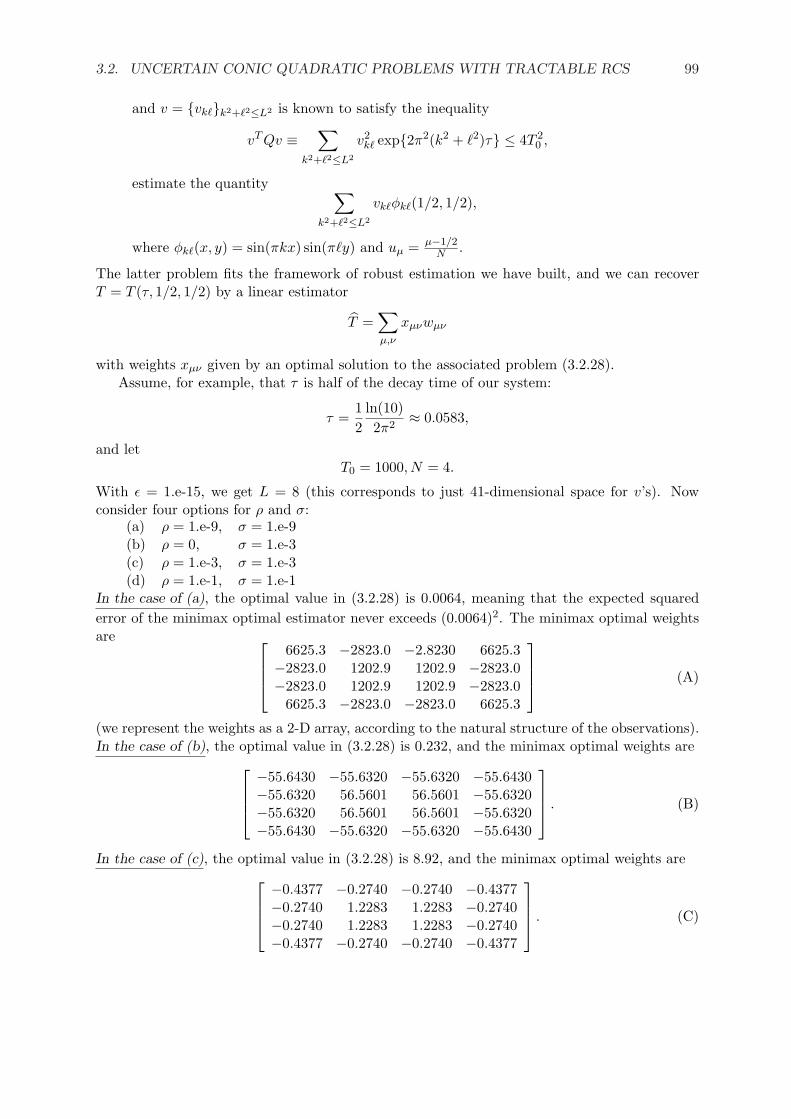
With ε = 1.e-15, we get L = 8 (this corresponds to just 41-dimensional space for v’s). Nowconsider four options for ρ and σ:
(a) ρ = 1.e-9, σ = 1.e-9(b) ρ = 0, σ = 1.e-3(c) ρ = 1.e-3, σ = 1.e-3(d) ρ = 1.e-1, σ = 1.e-1
In the case of (a), the optimal value in (3.2.28) is 0.0064, meaning that the expected squarederror of the minimax optimal estimator never exceeds (0.0064)2. The minimax optimal weightsare
6625.3 −2823.0 −2.8230 6625.3−2823.0 1202.9 1202.9 −2823.0−2823.0 1202.9 1202.9 −2823.0
6625.3 −2823.0 −2823.0 6625.3
(A)
(we represent the weights as a 2-D array, according to the natural structure of the observations).In the case of (b), the optimal value in (3.2.28) is 0.232, and the minimax optimal weights are
−55.6430 −55.6320 −55.6320 −55.6430−55.6320 56.5601 56.5601 −55.6320−55.6320 56.5601 56.5601 −55.6320−55.6430 −55.6320 −55.6320 −55.6430
. (B)
In the case of (c), the optimal value in (3.2.28) is 8.92, and the minimax optimal weights are
−0.4377 −0.2740 −0.2740 −0.4377−0.2740 1.2283 1.2283 −0.2740−0.2740 1.2283 1.2283 −0.2740−0.4377 −0.2740 −0.2740 −0.4377
. (C)

100 LECTURE 3: ROBUST CONIC OPTIMIZATION
In the case of (d), the optimal value in (3.2.28) is 63.9, and the minimax optimal weights are
0.1157 0.2795 0.2795 0.11570.2795 0.6748 0.6748 0.27950.2795 0.6748 0.6748 0.27950.1157 0.2795 0.2795 0.1157
. (D)
Now, in reality we can hardly know exactly the bounds ρ, σ on the measurement errors.What happens when we under- or over-estimate these quantities? To get an orientation, letus use every one of the weights given by (A), (B), (C), (D) in every one of the situations (a),(b), (c), (d). This is what happens with the errors (obtained as the average of observed errorsover 100 random simulations using the “nearly worst-case” signal v and “nearly worst-case”perturbation matrix ∆):
(a) (b) (c) (d)(A) 0.001 18.0 6262.9 6.26e5(B) 0.063 0.232 89.3 8942.7(C) 8.85 8.85 8.85 108.8(D) 8.94 8.94 8.94 63.3
We clearly see that, first, in our situation taking into account measurement errors, even prettysmall ones, is a must (this is so in all ill-posed estimation problems — those where the conditionnumber of Bn is large). Second, we see that underestimating the magnitude of measurementerrors seems to be much more dangerous than overestimating them.
3.3 Approximating RCs of Uncertain Conic Quadratic Prob-lems
In this section we focus on tight tractable approximations of uncertain CQIs — those withtightness factor independent (or nearly so) of the “size” of the description of the perturbationset. Known approximations of this type deal with side-wise uncertainty and two types of theleft hand side perturbations: the first is the case of structured norm-bounded perturbationsto be considered in section 3.3.1, while the second is the case of ∩-ellipsoidal left hand sideperturbation sets to be considered in section 3.3.2.
3.3.1 Structured Norm-Bounded Uncertainty
Consider the case where the uncertainty in CQI (3.2.3) is side-wise with the right hand sideuncertainty as in section 3.2.2, and with structured norm-bounded left hand side uncertainty,meaning that
1. The left hand side perturbation set is
Z leftρ = ρZ left
1 =
η = (η1, ..., ηN ) :ην ∈ Rpν×qν ∀ν ≤ N
‖ην‖2,2 ≤ ρ ∀ν ≤ N
ην = θνIpν , θν ∈ R, ν ∈ Is
(3.3.1)
Here Is is a given subset of the index set 1, ..., N such that pν = qν for ν ∈ Is.

3.3. APPROXIMATING RCS OF UNCERTAIN CONIC QUADRATIC PROBLEMS 101
Thus, the left hand side perturbations η ∈ Z left1 are block-diagonal matrices with pν × qν
diagonal blocks ην , ν = 1, ..., N . All of these blocks are of matrix norm not exceeding 1,and, in addition, prescribed blocks should be proportional to the unit matrices of appro-priate sizes. The latter blocks are called scalar, and the remaining — full perturbationblocks.
2. We have
A(η)y + b(η) = Any + bn +N∑
ν=1
LTν (y)ηνRν(y), (3.3.2)
where all matrices Lν(y) 6≡ 0, Rν(y) 6≡ 0 are affine in y and for every ν, either Lν(y), orRν(y), or both are independent of y.
Remark 3.1 W.l.o.g., we assume from now on that all scalar perturbation blocks are of the size1× 1: pν = qν = 1 for all ν ∈ Is.To see that this assumption indeed does not restrict generality, note that if ν ∈ Is, then inorder for (3.3.2) to make sense, Rν(y) should be a pν × 1 vector, and Lν(y) should be a pν × kmatrix, where k is the dimension of b(η). Setting Rν(y) ≡ 1, Lν(y) = RT
ν (y)Lν(y), observe thatLν(y) is affine in y, and the contribution θνL
Tν (y)Rν(y) of the ν-th scalar perturbation block
to A(η)y + b(η) is exactly the same as if this block were of size 1 × 1, and the matrices Lν(y),Rν(y) were replaced with Lν(y), Rν(y), respectively.
Note that Remark 3.1 is equivalent to the assumption that there are no scalar perturbationblocks at all — indeed, 1×1 scalar perturbation blocks can be thought of as full ones as well. 3.
Recall that we have already considered the particular case N = 1 of the uncertainty structure.Indeed, with a single perturbation block, that, as we just have seen, we can treat as a full one,we find ourselves in the situation of side-wise uncertainty with unstructured norm-bounded lefthand side perturbation (section 3.2.3). In this situation the RC of the uncertain CQI in questionis computationally tractable. The latter is not necessarily the case for general (N > 1) structurednorm-bounded left hand side perturbations. To see that the general structured norm-boundedperturbations are difficult to handle, note that they cover, in particular, the case of intervaluncertainty, where Z left
1 is the box η ∈ RL : ‖η‖∞ ≤ 1 and A(η), b(η) are arbitrary affinefunctions of η.
Indeed, the interval uncertainty
A(η)y + b(η) = [Any + bn] +N∑
ν=1ην [Aνy + bν ]
= [Any + bn] +N∑
ν=1[Aνy + bν ]︸ ︷︷ ︸
LTν (y)
·ην · 1︸︷︷︸Rν(y)
,(3.3.3)
is nothing but the structured norm-bounded perturbation with 1 × 1 perturbationblocks.
From the beginning of section 3.1.3 we know that the RC of uncertain CQI with side-wise un-certainty and interval uncertainty in the left hand side in general is computationally intractable,meaning that structural norm-bounded uncertainty can be indeed difficult.
3A reader could ask, why do we need the scalar perturbation blocks, given that finally we can get rid of themwithout loosing generality. The answer is, that we intend to use the same notion of structured norm-boundeduncertainty in the case of uncertain LMIs, where Remark 3.1 does not work.

102 LECTURE 3: ROBUST CONIC OPTIMIZATION
Approximating the RC of Uncertain Least Squares Inequality
We start with deriving a safe tractable approximation of the RC of an uncertain Least Squaresconstraint
‖A(η)y + b(η)‖2 ≤ τ, (3.3.4)
with structured norm-bounded perturbation (3.3.1), (3.3.2).Step 1: reformulating the RC of (3.3.4), (3.3.1), (3.3.2) as a semi-infinite LMI. Givena k-dimensional vector u (k is the dimension of b(η)) and a real τ , let us set
Arrow(u, t) =[
τ uT
u τIk
].
Recall that by Lemma 3.1 ‖u‖2 ≤ τ if and only if Arrow(u, τ) º 0. It follows that the RC of(3.3.4), (3.3.1), (3.3.2), which is the semi-infinite Least Squares inequality
‖A(η)y + b(η)‖2 ≤ τ ∀η ∈ Z leftρ ,
can be rewritten asArrow(A(η)y + b(η), τ) º 0 ∀η ∈ Z left
ρ . (3.3.5)
Introducing k × (k + 1) matrix L = [0k×1, Ik] and 1× (k + 1) matrix R = [1, 0, ..., 0], we clearlyhave
Arrow(A(η)y + b(η), τ) = Arrow(Any + bn, τ)
+N∑
ν=1
[LT LTν (y)ηνRν(y)R+RT RT
ν (y)[ην ]T Lν(y)L].
(3.3.6)
Now, since for every ν, either Lν(y), or Rν(y), or both, are independent of y, renaming, ifnecessary [ην ]T as ην , and swapping Lν(y)L and Rν(y)R, we may assume w.l.o.g. that in therelation (3.3.6) all factors Lν(y) are independent of y, so that the relation reads
Arrow(A(η)y + b(η), τ) = Arrow(Any + bn, τ)
+N∑
ν=1
[LT LTν︸ ︷︷ ︸
LTν
ην Rν(y)R︸ ︷︷ ︸Rν(y)
+RTν (y)[ην ]T Lν
]
where Rν(y) are affine in y and Lν 6= 0. Observe also that all the symmetric matrices
Bν(y, ην) = LTν ηνRν(y) + RT
ν (y)[ην ]T Lν
are differences of two matrices of the form Arrow(u, τ) and Arrow(u′, τ), so that these arematrices of rank at most 2. The intermediate summary of our observations is as follows:
(#): The RC of (3.3.4), (3.3.1), (3.3.2) is equivalent to the semi-infinite LMI
Arrow(Any + bn, τ)︸ ︷︷ ︸B0(y,τ)
+N∑
ν=1Bν(y, ην) º 0 ∀
(η :
ην ∈ Rpν×qν ,‖ην‖2,2 ≤ ρ ∀ν ≤ N
)
[Bν(y, ην) = LT
ν ηνRν(y) + RTν (y)[ην ]T Lν , ν = 1, ..., N
pν = qν = 1∀ν ∈ Is
](3.3.7)
Here R(y) are affine in y, and for all y, all ν ≥ 1 and all ην the ranks of the matrices Bν(y, ην)do not exceed 2.

3.3. APPROXIMATING RCS OF UNCERTAIN CONIC QUADRATIC PROBLEMS 103
Step 2. Approximating (3.3.7). Observe that an evident sufficient condition for the validityof (3.3.7) for a given y is the existence of symmetric matrices Yν , ν = 1, ..., N , such that
Yν º Bν(y, ην)∀ (ην ∈ Zν = ην : ‖ην‖2,2 ≤ 1; ν ∈ Is ⇒ ην ∈ RIpν) (3.3.8)
and
B0(y, τ)− ρN∑
ν=1
Yν º 0. (3.3.9)
We are about to demonstrate that the semi-infinite LMIs (3.3.8) in variables Yν , y, τ can berepresented by explicit finite systems of LMIs, so that the system S0 of semi-infinite constraints(3.3.8), (3.3.9) on variables Y1, ..., YN , y, τ is equivalent to an explicit finite system S of LMIs.Since S0, due to its origin, is a safe approximation of (3.3.7), so will be S, (which, in addition,is tractable). Now let us implement our strategy.
10. Let us start with ν ∈ Is. Here (3.3.8) clearly is equivalent to just two LMIs
Yν º Bν(y) ≡ LTν Rν(y) + RT
ν (y)Lν & Yν º −Bν(y). (3.3.10)
20. Now consider relation (3.3.8) for the case ν 6∈ Is. Here we have
(Yν , y) satisfies (3.3.8)
⇔ uT Yνu ≥ uT Bν(y, ην)u ∀u∀(ην : ‖ην‖2,2 ≤ 1)
⇔ uT Yνu ≥ uT LTν ηνRν(y)u + uT RT
ν (y)[ην ]T Lνu ∀u∀(ην : ‖ην‖2,2 ≤ 1)
⇔ uT Yνu ≥ 2uT LTν ηνRν(y)u ∀u∀(ην : ‖ην‖2,2 ≤ 1)
⇔ uT Yνu ≥ 2‖Lνu‖2‖R(y)u‖2 ∀u⇔ uT Yνu− 2ξT Rν(y)u ∀(u, ξ : ξT ξ ≤ uT LT
ν Lνu)
Invoking the S-Lemma, the concluding condition in the latter chain is equivalent to
∃λν ≥ 0 :
[Yν − λνL
Tν Lν −RT
ν (y)−Rν(y) λνIkν
]º 0, (3.3.11)
where kν is the number of rows in Rν(y).We have proved the first part of the following statement:
Theorem 3.4 The explicit system of LMIs
Yν º ±(LTν Rν(y) + RT
ν (y)Lν), ν ∈ Is[Yν − λνL
Tν Lν RT
ν (y)Rν(y) λνIkν
]º 0, ν 6∈ Is
Arrow(Any + bn, τ)− ρN∑
ν=1Yν º 0
(3.3.12)
(for notation, see (3.3.7)) in variables Y1, ..., YN , λν , y, τ is a safe tractable approximation of theRC of the uncertain Least Squares inequality (3.3.4), (3.3.1), (3.3.2). The tightness factor of thisapproximation never exceeds π/2, and equals to 1 when N = 1.

104 LECTURE 3: ROBUST CONIC OPTIMIZATION
Proof. By construction, (3.3.12) indeed is a safe tractable approximation of the RC of (3.3.4),
(3.3.1), (3.3.2) (note that a matrix of the form[
A BBT A
]is º 0 if and only if the matrix
[A −B
−BT A
]is so). By Remark and Theorem 3.2, our approximation is exact when N = 1.
The fact that the tightness factor never exceeds π/2 is an immediate corollary of the real caseMatrix Cube Theorem (Theorem A.7), and we use the corresponding notation in the rest of theproof. Observe that a given pair (y, τ) is robust feasible for (3.3.4), (3.3.1), (3.3.2) if and onlyif the matrices B0 = B0(y, τ), Bi = Bνi(y, 1), i = 1, ..., p, Lj = Lµj , Rj = Rµj (y), j = 1, ..., q,satisfy A(ρ); here Is = ν1 < ... < νp and 1, ..., L\Is = µ1 < ... < µq. At the same time,the validity of the corresponding predicate B(ρ) is equivalent to the possibility to extend y to asolution of (3.3.12) due to the origin of the latter system. Since all matrices Bi, i = 1, ..., p, areof rank at most 2 by (#), the Matrix Cube Theorem implies that if (y, τ) cannot be extended toa feasible solution to (3.3.12), then (y, τ) is not robust feasible for (3.3.4), (3.3.1), (3.3.2) whenthe uncertainty level is increased by the factor ϑ(2) = π
2 . ¤Illustration: Antenna Design revisited. Consider the Antenna Design example (Example1.1) and assume that instead of measuring the closeness of a synthesized diagram to the targetone in the uniform norm, as was the case in section 1.1.3, we want to use the Euclidean norm,specifically, the weighted 2-norm
‖f(·)‖2,w =
(m∑
i=1
f2(θi)µi
)1/2
[θi = iπ2m , 1 ≤ i ≤ m = 240, µi = cos(θi)∑m
s=1 cos(θs)]
To motivate the choice of weights, recall that the functions f(·) we are interested in arerestrictions of diagrams (and their differences) on the equidistant L-point grid of altitudeangles. The diagrams in question are, physically speaking, functions of a 3D direction fromthe upper half-space (a point on the unit 2D hemisphere) which depend solely on the altitudeangle and are independent of the longitude angle. A “physically meaningful” L2-norm herecorresponds to uniform distribution on the hemisphere; after discretization of the altitudeangle, this L2 norm becomes our ‖ · ‖2.
with this measure of discrepancy between a synthesized and the target diagram, the problem ofinterest becomes the uncertain problem
miny,τ
τ : ‖WD[I + Diagη]y − b‖2 ≤ τ : η ∈ ρZ
, Z = η ∈ RL=10 : ‖η‖∞ ≤ 1, (3.3.13)
where
• D = [Dij = Dj(θi)] 1≤i≤m=240,1≤j≤L=10
] is the matrix comprised of the diagrams of L = 10 antenna
elements (central circle and surrounding rings), see section 1.1.3,
• W = Diag√µ1, ...,√
µm, so that ‖Wz‖2 = ‖z‖2,w, and b = W [D∗(θ1); ...; D∗(θm)] comesfrom the target diagram D∗(·), and
• η is comprised of actuation errors, and ρ is the uncertainty level.
Nominal design. Solving the nominal problem (corresponding to ρ = 0), we end up with thenominal optimal design which “in the dream” – with no actuation errors – is really nice (figure

3.3. APPROXIMATING RCS OF UNCERTAIN CONIC QUADRATIC PROBLEMS 105
0 10 20 30 40 50 60 70 80 90−0.2
0
0.2
0.4
0.6
0.8
1
1.2
0 10 20 30 40 50 60 70 80 90−6
−4
−2
0
2
4
6
8
0 10 20 30 40 50 60 70 80 90−60
−40
−20
0
20
40
60
0 10 20 30 40 50 60 70 80 90−600
−400
−200
0
200
400
600
ρ = 0 ρ = 0.0001 ρ = 0.001 ρ = 0.01
Figure 3.1: “Dream and reality,” nominal optimal design: samples of 100 actual diagrams (red)for different uncertainty levels. Blue: the target diagram
Dream Realityρ = 0 ρ = 0.0001 ρ = 0.001 ρ = 0.01value min mean max min mean max min mean max
‖ · ‖2,w-distanceto target
0.011 0.077 0.424 0.957 1.177 4.687 9.711 8.709 45.15 109.5
energyconcentration
99.4% 0.23% 20.1% 77.7% 0.70% 19.5% 61.5% 0.53% 18.9% 61.5%
Table 3.1: Quality of nominal antenna design: dream and reality. Data over 100 samples ofactuation errors per each uncertainty level ρ.
3.1, case of ρ = 0): the ‖ · ‖2,w-distance of the nominal diagram to the target is as small as0.0112, and the energy concentration for this diagram is as large as 99.4%. Unfortunately, thedata in figure 3.1 and table 3.1 show that “in reality,” with the uncertainty level as small asρ = 0.01%, the nominal design is a complete disaster.
Robust design. Let us build a robust design. The set Z is a unit box, that is, we are inthe case of interval uncertainty, or, which the same, structured norm-bounded uncertainty withL = 10 scalar perturbation blocks η`. Denoting `-th column of WD by [WD]`, we have
WD[I + Diagη]y − b = [WDy − b] +L∑
`=1
η` [y`[WD]`] ,
that is, taking into account (3.3.3), we have in the notation of (3.3.2):
Any + bn = WDy − b, Lν(y) = yν [WD]Tν , ην ≡ ην , Rν(y) ≡ 1, 1 ≤ ν ≤ N ≡ L = 10,
so that in the notation of Theorem 3.4 we have
Rν(y) = [0, yν [WD]Tν ], Lν = [1, 01×n], kν = 1, ., 1 ≤ ν ≤ N ≡ L.
Since we are in our right to treat all perturbation blocks as scalar, a tight within the factor π/2safe tractable approximation, given by Theorem 3.4, of the RC of our uncertain Least Squares

106 LECTURE 3: ROBUST CONIC OPTIMIZATION
problem reads
minτ,y,Y1,...,YL
τ : Arrow(WDy − b, τ)− ρ
L∑
ν=1
Yν º 0, Yν º ±[LT
ν Rν(y) + RTν (y)Lν
], 1 ≤ ν ≤ L
.
(3.3.14)This problem simplifies dramatically due to the following simple fact (see Exercise 3.6):
(!) Let a, b be two vectors of the same dimension with a 6= 0. Then Y º abT + baT
if and only if there exists λ ≥ 0 such that Y º λaaT + 1λbbT .
Here, by definition, 10bbT is undefined when b 6= 0 and is the zero matrix when b = 0.
By (!), a pair (τ, y) can be extended, by properly chosen Yν , ν = 1, ..., L, to a feasible solutionof (3.3.14) if and only if there exist λν ≥ 0, 1 ≤ ν ≤ L, such that Arrow(WDy − b, τ) −ρ
∑ν
[λνL
Tν Lν + λ−1
ν RTν (y)Rν(y)
]º 0, which, by the Schur Complement Lemma is equivalent
to [Arrow(WDy − b, τ)−∑
νρλνL
Tν Lν ρ[RT
1 (y), ..., RTL(y)]
ρ[R1(y); ...; RL(y)] ρDiagλ1, ..., λL
]º 0.
Thus, problem (3.3.14) is equivalent to
minτ,y,γ
τ :
[Arrow(WDy − b, τ)−∑
νγνL
Tν Lν ρ[RT
1 (y), ..., RTL(y)]
ρ[R1(y); ...; RL(y)] Diagγ1, ..., γL
]º 0
(3.3.15)
(we have set γν = ρλν). Note that we managed to replace every matrix variable Yν in (3.3.14)with a single scalar variable λν in (3.3.15). Note that this dramatic simplification is possiblewhenever all perturbation blocks are scalar.
With our particular Lν and Rν(y) the resulting problem (3.3.15) reads
minτ,y,γ
τ :
τ −∑Lν=1 γν [WDy − b]T
WDy − b τIm ρ[y1[WD]1, ..., yL[WD]L]ρ[y1[WD]1, ..., yL[WD]L]T Diagγ1, ..., γL
º 0
.
(3.3.16)We have solved (3.3.16) at the uncertainty level ρ = 0.01, thus getting a robust design.
The optimal value in (3.3.16) is 0.02132 – while being approximately 2 times worse than thenominal optimal value, it still is pretty small. We then tested the robust design against actuationerrors of magnitude ρ = 0.01 and larger. The results, summarized in figure 3.2 and table 3.2,allow for the same conclusions as in the case of LP-based design, see p. 22. Recall that(3.3.16) is not the “true” RC of our uncertain problem, is just a safe approximation, tightwithin the factor π/2, of this RC. All we can conclude from this is that the value τ∗ = 0.02132of τ yielded by the approximation (that is, the guaranteed value of the objective at our robustdesign, the uncertainty level being 0.01) is in-between the true robust optimal values Opt∗(0.01)and Opt∗(0.01π/2) at the uncertainty levels 0.01 and 0.01π/2, respectively. This informationdoes not allow for meaningful conclusions on how far away is τ∗ from the true robust optimalvalue Opt∗(0.01); at this point, all we can say in this respect is that Opt∗(0, 01) is at leastthe nominal optimal value Opt∗(0) = 0.0112, and thus the loss in optimality caused by ourapproximation is at most by factor τ∗/Opt∗(0) = 1.90. In particular, we cannot exclude thatwith our approximation, we lose as much as 90% in the value of the objective. The reality,however, is by far not so bad. Note that our perturbation set – the 10-dimensional box – is a

3.3. APPROXIMATING RCS OF UNCERTAIN CONIC QUADRATIC PROBLEMS 107
0 10 20 30 40 50 60 70 80 90−0.2
0
0.2
0.4
0.6
0.8
1
1.2
0 10 20 30 40 50 60 70 80 90−0.2
0
0.2
0.4
0.6
0.8
1
1.2
0 10 20 30 40 50 60 70 80 90−0.2
0
0.2
0.4
0.6
0.8
1
1.2
ρ = 0.01 ρ = 0.05 ρ = 0.1
Figure 3.2: “Dream and reality,” robust optimal design: samples of 100 of actual diagrams (red)for different uncertainty levels. Blue: the target diagram.
Realityρ = 0.01 ρ = 0.05 ρ = 0.1
min mean max min mean max min mean max‖ · ‖2,w-distance
to target0.021 0.021 0.021 0.021 0.023 0.030 0.021 0.030 0.048
energyconcentration
96.5% 96.7% 96.9% 93.0% 95.8% 96.8% 80.6% 92.9% 96.7%
Table 3.2: Quality of robust antenna design. Data over 100 samples of actuation errors per eachuncertainty level ρ.For comparison: for nominal design, with the uncertainty level as small as ρ = 0.001, theaverage ‖ · ‖2,w-distance of the actual diagram to target is as large as 4.69, and the expectedenergy concentration is as low as 19.5%.

108 LECTURE 3: ROBUST CONIC OPTIMIZATION
convex hull of 1024 vertices, so we can think about our uncertainty as of the scenario one (section3.2.1) generated by 1024 scenarios. This number is still within the grasp of the straightforwardscheme proposed in section 3.2.1, and thus we can find in a reasonable time the true robustoptimal value Opt∗(0.01), which turns out to be 0.02128. We see that the actual loss in thevalue of the objective caused by approximation its really small – it is less than 0.2%.
Least Squares Inequality with Structured Norm-Bounded Uncertainty, ComplexCase
The uncertain Least Squares inequality (3.3.4) with structured norm-bounded perturbationsmakes sense in the case of complex left hand side data as well as in the case of real data.Surprisingly, in the complex case the RC admits a better in tightness factor safe tractableapproximation than in the real case (specifically, the tightness factor π
2 = 1.57... stated inTheorem 3.4 in the complex case improves to 4
π = 1.27...). Consider an uncertain Least Squaresinequality (3.3.4) where A(η) ∈ Cm×n, b(η) ∈ Cm and the perturbations are structured norm-bounded and complex, meaning that (cf. (3.3.1), (3.3.2))
(a) Z leftρ = ρZ left
1 =
η = (η1, ..., ηN ) :
ην ∈ Cpν×qν , ν = 1, ..., N
‖ην‖2,2 ≤ ρ, ν = 1, ..., N
ην = θνIpν , θν ∈ C, ν ∈ Is
,
(b) A(ζ)y + b(ζ) = [Any + bn] +N∑
ν=1LH
ν (y)ηνRν(y),
(3.3.17)
where Lν(y), Rν(y) are affine in [<(y);=(y)] matrices with complex entries such that for every νat least one of these matrices is independent on y and is nonzero, and BH denotes the Hermitianconjugate of a complex-valued matrix B: (BH)ij = Bji, where z is the complex conjugate of acomplex number z.
Observe that by exactly the same reasons as in the real case, we can assume w.l.o.g. thatall scalar perturbation blocks are 1 × 1, or, equivalently, that there are no scalar perturbationblocks at all, so that from now on we assume that Is = ∅.
The derivation of the approximation is similar to the one in the real case. Specifically, westart with the evident observation that for a complex k-dimensional vector u and a real t therelation
‖u‖2 ≤ t
is equivalent to the fact that the Hermitian matrix
Arrow(u, t) =[
t uH
u tIk
]
is º 0; this fact is readily given by the complex version of the Schur Complement Lemma:
a Hermitian block matrix
[P QH
Q R
]with R Â 0 is positive semidefinite if and only if the
Hermitian matrix P −QHR−1Q is positive semidefinite (cf. the proof of Lemma 3.1). It followsthat (y, τ) is robust feasible for the uncertain Least Squares inequality in question if and only if
Arrow(Any + bn, τ)︸ ︷︷ ︸B0(y,τ)
+N∑
ν=1Bν(y, ην) º 0∀ (η : ‖ην‖2,2 ≤ ρ∀ν ≤ N)
[Bν(y, ην) = LH
ν ηνRν(y) + RHν (y)[ην ]HLν , ν = 1, ..., N
] (3.3.18)

3.3. APPROXIMATING RCS OF UNCERTAIN CONIC QUADRATIC PROBLEMS 109
where Lν are constant matrices, and R(y) are affine in [<(y);=(y)] matrices readily given byLν(y), Rν(y) (cf. (3.3.7) and take into account that we are in the situation Is = ∅). It followsthat whenever, for a given (y, τ), one can find Hermitian matrices Yν such that
Yν º Bν(y, ην) ∀(ην ∈ Cpν×qν : ‖ην‖2,2 ≤ 1), ν = 1, ..., N, (3.3.19)
and B0(y, τ) º ρN∑
ν=1Yν , the pair (y, τ) is robust feasible.
Same as in the real case, applying the S-Lemma, (which works in the complex case as well asin the real one), a matrix Yν satisfies (3.3.19) if and only if
∃λν ≥ 0 :
[Yν − λνL
Hν Lν −RH
ν (y)−Rν(y) λνIkν
],
where kν is the number of rows in Rν(y). We have arrived at the first part of the followingstatement:
Theorem 3.5 The explicit system of LMIs
[Yν − λνL
Hν Lν RH
ν (y)Rν(y) λνIkν
]º 0, ν = 1, ..., N,
Arrow(Any + bn, τ)− ρN∑
ν=1Yν º 0
(3.3.20)
(for notation, see (3.3.18)) in the variables Yi = Y Hi , λν , y, τ is a safe tractable approximation
of the RC of the uncertain Least Squares inequality (3.3.4), (3.3.17). The tightness factor of thisapproximation never exceeds 4/π, and is equal to 1 when N = 1.
Proof is completely similar to the one of Theorem 3.4, modulo replacing the real case of theMatrix Cube Theorem (Theorem A.7) with its complex case (Theorem A.6).
From Uncertain Least Squares to Uncertain CQI
Let us come back to the real case. We have already built a tight approximation for the RCof a Least Squares inequality with structured norm-bounded uncertainty in the left hand sidedata. Our next goal is to extend this approximation to the case of uncertain CQI with side-wiseuncertainty.
Theorem 3.6 Consider the uncertain CQI (3.2.3) with side-wise uncertainty, where the lefthand side uncertainty is the structured norm-bounded one given by (3.3.1), (3.3.2), and the righthand side perturbation set is given by a conic representation (cf. Theorem 1.1)
Zrightρ = ρZright
1 , Zright1 = χ : ∃u : Pχ + Qu + p ∈ K , (3.3.21)
where 0 ∈ Zright1 , K is a closed convex pointed cone and the representation is strictly feasible
unless K is a polyhedral cone given by an explicit finite list of linear inequalities, and 0 ∈ Zright1 .

110 LECTURE 3: ROBUST CONIC OPTIMIZATION
For ρ > 0, the explicit system of LMIs
(a) τ + ρpT v ≤ δ(y), P T v = σ(y), QT v = 0, v ∈ K∗
(b.1) Yν º ±(LTν Rν(y) + RT
ν (y)Lν), ν ∈ Is
(b.2)
[Yν − λνL
Tν Lν RT
ν (y)Rν(y) λνIkν
]º 0, ν 6∈ Is
(b.3) Arrow(Any + bn, τ)− ρN∑
ν=1Yν º 0
(3.3.22)
(for notation, see (3.3.7)) in variables Y1, ..., YN , λν , y, τ, v is a safe tractable approximation ofthe RC of (3.2.4). This approximation is exact when N = 1, and is tight within the factor π
2otherwise.
Proof. Since the uncertainty is side-wise, y is robust feasible for (3.2.4), (3.3.1), (3.3.2), (3.3.21),the uncertainty level being ρ > 0, if and only if there exists τ such that
(c) σT (χ)y + δ(χ) ≥ τ ∀χ ∈ ρZright1 ,
(d) ‖A(η)y + b(η)‖2 ≤ τ ∀η ∈ ρZ left1 .
When ρ > 0, we have
ρZright1 = χ : ∃u : P (χ/ρ) + Qu + p ∈ K = χ : ∃u′ : Pχ + Qu′ + ρp ∈ K;
from the resulting conic representation of ρZright1 , same as in the proof of Theorem 1.1, we
conclude that the relations (3.3.22.a) represent equivalently the requirement (c), that is, (y, τ)satisfies (c) if and only if (y, τ) can be extended, by properly chosen v, to a solution of (3.3.22.a).By Theorem 3.4, the possibility to extend (y, τ) to a feasible solution of (3.3.22.b) is a sufficientcondition for the validity of (d). Thus, the (y, τ) component of a feasible solution to (3.3.22)satisfies (c), (d), meaning that y is robust feasible at the level of uncertainty ρ. Thus, (3.3.22)is a safe approximation of the RC in question.
The fact that the approximation is precise when there is only one left hand side perturbationblock is readily given by Theorem 3.2 and Remark 3.1 allowing us to treat this block as full.It remains to verify that the tightness factor of the approximation is at most π
2 , that is, tocheck that if a given y cannot be extended to a feasible solution of the approximation for theuncertainty level ρ, then y is not robust feasible for the uncertainty level π
2 ρ (see comments afterDefinition 3.3). To this end, let us set
τy(r) = infχ
σT (χ)y + δ(χ) : χ ∈ rZright
1
.
Since 0 ∈ Zright1 by assumption, τy(r) is nonincreasing in r. Clearly, y is robust feasible at the
uncertainty level r if and only if
‖A(η)y + b(η)‖2 ≤ τy(r) ∀η ∈ rZ left1 . (3.3.23)
Now assume that a given y cannot be extended to a feasible solution of (3.3.22) for the uncer-tainty level ρ. Let us set τ = τy(ρ); then (y, τ) can be extended, by a properly chosen v, toa feasible solution of (3.3.22.a). Indeed, the latter system expresses equivalently the fact that
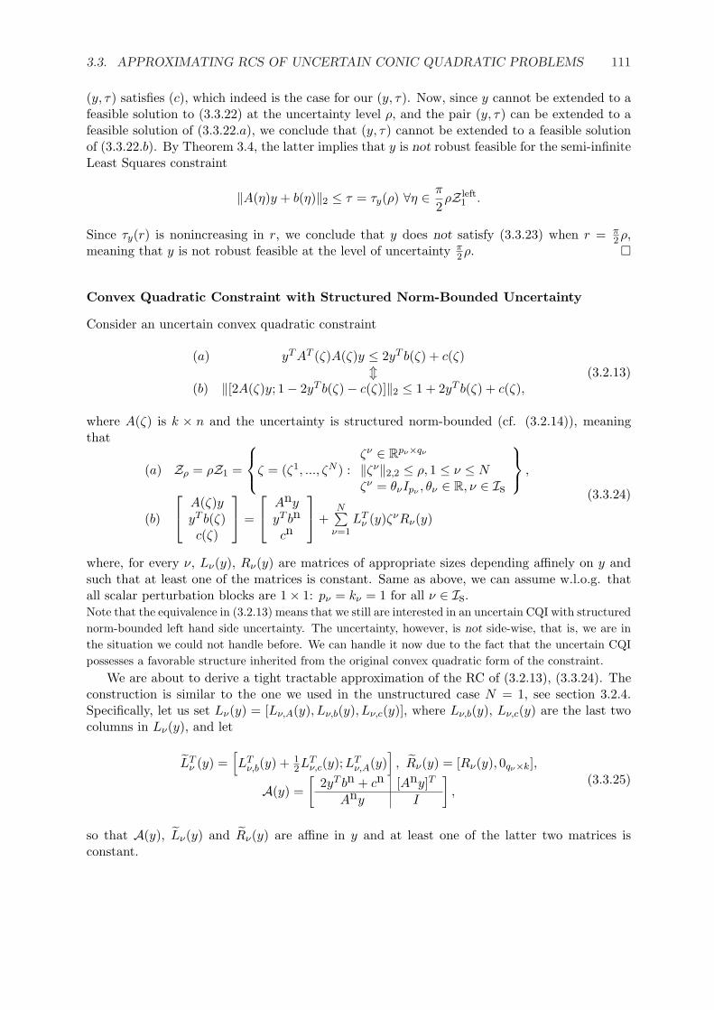
3.3. APPROXIMATING RCS OF UNCERTAIN CONIC QUADRATIC PROBLEMS 111
(y, τ) satisfies (c), which indeed is the case for our (y, τ). Now, since y cannot be extended to afeasible solution to (3.3.22) at the uncertainty level ρ, and the pair (y, τ) can be extended to afeasible solution of (3.3.22.a), we conclude that (y, τ) cannot be extended to a feasible solutionof (3.3.22.b). By Theorem 3.4, the latter implies that y is not robust feasible for the semi-infiniteLeast Squares constraint
‖A(η)y + b(η)‖2 ≤ τ = τy(ρ) ∀η ∈ π
2ρZ left
1 .
Since τy(r) is nonincreasing in r, we conclude that y does not satisfy (3.3.23) when r = π2 ρ,
meaning that y is not robust feasible at the level of uncertainty π2 ρ. ¤
Convex Quadratic Constraint with Structured Norm-Bounded Uncertainty
Consider an uncertain convex quadratic constraint
(a) yT AT (ζ)A(ζ)y ≤ 2yT b(ζ) + c(ζ)m
(b) ‖[2A(ζ)y; 1− 2yT b(ζ)− c(ζ)]‖2 ≤ 1 + 2yT b(ζ) + c(ζ),(3.2.13)
where A(ζ) is k × n and the uncertainty is structured norm-bounded (cf. (3.2.14)), meaningthat
(a) Zρ = ρZ1 =
ζ = (ζ1, ..., ζN ) :
ζν ∈ Rpν×qν
‖ζν‖2,2 ≤ ρ, 1 ≤ ν ≤ Nζν = θνIpν , θν ∈ R, ν ∈ Is
,
(b)
A(ζ)yyT b(ζ)c(ζ)
=
AnyyT bn
cn
+
N∑ν=1
LTν (y)ζνRν(y)
(3.3.24)
where, for every ν, Lν(y), Rν(y) are matrices of appropriate sizes depending affinely on y andsuch that at least one of the matrices is constant. Same as above, we can assume w.l.o.g. thatall scalar perturbation blocks are 1× 1: pν = kν = 1 for all ν ∈ Is.Note that the equivalence in (3.2.13) means that we still are interested in an uncertain CQI with structurednorm-bounded left hand side uncertainty. The uncertainty, however, is not side-wise, that is, we are inthe situation we could not handle before. We can handle it now due to the fact that the uncertain CQIpossesses a favorable structure inherited from the original convex quadratic form of the constraint.
We are about to derive a tight tractable approximation of the RC of (3.2.13), (3.3.24). Theconstruction is similar to the one we used in the unstructured case N = 1, see section 3.2.4.Specifically, let us set Lν(y) = [Lν,A(y), Lν,b(y), Lν,c(y)], where Lν,b(y), Lν,c(y) are the last twocolumns in Lν(y), and let
LTν (y) =
[LT
ν,b(y) + 12LT
ν,c(y);LTν,A(y)
], Rν(y) = [Rν(y), 0qν×k],
A(y) =[
2yT bn + cn [Any]T
Any I
],
(3.3.25)
so that A(y), Lν(y) and Rν(y) are affine in y and at least one of the latter two matrices isconstant.

112 LECTURE 3: ROBUST CONIC OPTIMIZATION
We have
yT AT (ζ)A(ζ)y ≤ 2yT b(ζ) + c(ζ) ∀ζ ∈ Zρ
⇔[
2yT b(ζ) + c(ζ) [A(ζ)y]T
A(ζ)y I
]º 0 ∀ζ ∈ Zρ [Schur Complement Lemma]
⇔
A(y)︷ ︸︸ ︷[2yT bn + cn [Any]T
Any I
]
+N∑
ν=1
[[2Lν,b(y) + Lν,c(y)]T ζνRν(y) [LT
ν,A(y)ζνRν(y)]T
LTν,A(y)ζνRν(y)
]
︸ ︷︷ ︸=LT
ν (y)ζνRν(y)+RTν (y)[ζν ]T Lν(y)
º 0 ∀ζ ∈ Zρ
[by (3.3.24)]
⇔ A(y) +N∑
ν=1
[LT
ν (y)ζνRν(y) + RTν (y)[ζν ]T Lν(y)
]º 0 ∀ζ ∈ Zρ.
Taking into account that for every ν at least one of the matrices Lν(y), Rν(y) is independentof y and swapping, if necessary, ζν and [ζν ]T , we can rewrite the last condition in the chain as
A(y) +N∑
ν=1
[LT
ν ζνRν(y) + RTν (y)[ζν ]T Lν
]º 0 ∀(ζ : ‖ζν‖2,2 ≤ ρ) (3.3.26)
where Lν , Rν(y) are readily given matrices and Rν(y) is affine in y. (Recall that we are inthe situation where all scalar perturbation blocks are 1× 1 ones, and we can therefore skip theexplicit indication that ζν = θνIpν for ν ∈ Is). Observe also that similarly to the case of a Least
Squares inequality, all matrices[LT
ν ζνRν(y) + RTν (y)[ζν ]T Lν
]are of rank at most 2. Finally, we
lose nothing by assuming that Lν are nonzero for all ν.Proceeding exactly in the same fashion as in the case of the uncertain Least Squares inequality
with structured norm-bounded perturbations, we arrive at the following result (cf. Theorem 3.4):
Theorem 3.7 The explicit system of LMIs
Yν º ±(LTν Rν(y) + RT
ν (y)Lν), ν ∈ Is[
Yν − λνLTν Lν RT
ν (y)Rν(y) λνIkν
]º 0, ν 6∈ Is
A(y)− ρL∑
ν=1Yν º 0
(3.3.27)
(kν is the number of rows in Rν) in variables Y1, ..., YN , λν , y is a safe tractable approximationof the RC of the uncertain convex quadratic constraint (3.2.13), (3.3.24). The tightness factorof this approximation never exceeds π/2, and equals 1 when N = 1.
Complex case. The situation considered in section 3.3.1 admits a complex data version aswell. Consider a convex quadratic constraint with complex-valued variables and a complex-

3.3. APPROXIMATING RCS OF UNCERTAIN CONIC QUADRATIC PROBLEMS 113
valued structured norm-bounded uncertainty:
yHAH(ζ)A(ζ)y ≤ <2yHb(ζ) + c(ζ)
ζ ∈ Zρ = ρZ1 =
ζ = (ζ1, ..., ζN ) :
ζν ∈ Cpν×qν , 1 ≤ ν ≤ N‖ζν‖2,2 ≤ ρ, 1 ≤ ν ≤ Nν ∈ Is ⇒ ζν = θνIpν , θν ∈ C
A(ζ)yyHb(ζ)c(ζ)
=
AnyyHbn
cn
+
N∑ν=1
LHν (y)ζνRν(y),
(3.3.28)
where An ∈ Ck×m and the matrices Lν(y), Rν(y) are affine in [<(y);=(y)] and such that forevery ν, either Lν(y), or Rν(y) are independent of y. Same as in the real case we have justconsidered, we lose nothing when assuming that all scalar perturbation blocks are 1× 1, whichallows us to treat these blocks as full. Thus, the general case can be reduced to the case whereIs = ∅, which we assume from now on (cf. section 3.3.1).
In order to derive a safe approximation of the RC of (3.3.28), we can act exactly in the samefashion as in the real case to arrive at the equivalence
yHAH(ζ)A(ζ)y ≤ <2yHb(ζ) + c(ζ) ∀ζ ∈ Zρ
⇔
A(y)︷ ︸︸ ︷[ <2yHbn + cn [Any]H
Any I
]
+N∑
ν=1
[ <2yHLν,b(y)ζνRν(y) + Lν,c(y)ζνRν(y) RHν [ζν ]HLν,A(y)
LHν,A(y)ζνRν(y)
]º 0
∀(ζ : ‖ζν‖2,2 ≤ ρ, 1 ≤ ν ≤ N)
where Lν(y) = [Lν,A(y), Lν,b(y), Lν,c(y)] and Lν,b(y), Lν,c(y) are the last two columns in Lν(y).Setting
LHν (y) =
[LH
ν,b(y) +12LH
ν,c(y);LHν,A(y)
], Rν(y) = [Rν(y), 0qν×k]
(cf. (3.3.25)), we conclude that the RC of (3.3.28) is equivalent to the semi-infinite LMI
A(y) +N∑
ν=1
[LH
ν (y)ζνRν(y) + RHν (y)[ζν ]HLν(y)
]º 0
∀(ζ : ‖ζν‖2,2 ≤ ρ, 1 ≤ ν ≤ N).(3.3.29)
As always, swapping, if necessary, ζν and [ζν ]H we may rewrite the latter semi-infinite LMIequivalently as
A(y) +N∑
ν=1
[LH
ν ζνRν(y) + RHν (y)[ζν ]HLν
]º 0
∀(ζ : ‖ζν‖2,2 ≤ ρ, 1 ≤ ν ≤ N),
where Rν(y) are affine in [<(y);=(y)] and Lν are nonzero. Applying the Complex case MatrixCube Theorem (see the proof of Theorem 3.5), we finally arrive at the following result:
Theorem 3.8 The explicit system of LMIs[
Yν − λνLHν Lν RH
ν (y)Rν(y) λνIkν
]º 0, ν = 1, ..., N,
[ <2yHbn + cn [Any]H
Any I
]− ρ
N∑ν=1
Yν º 0
(3.3.30)

114 LECTURE 3: ROBUST CONIC OPTIMIZATION
(kν is the number of rows in Rν(y)) in variables Y1 = Y H1 , ..., YN = Y H
N , λν ∈ R, y ∈ Cm isa safe tractable approximation of the RC of the uncertain convex quadratic inequality (3.3.28).The tightness of this approximation is ≤ 4
π , and is equal to 1 when N = 1.
3.3.2 The Case of ∩-Ellipsoidal Uncertainty
Consider the case where the uncertainty in CQI (3.2.3) is side-wise with the right hand sideuncertainty exactly as in section 3.2.2, and with ∩-ellipsoidal left hand side perturbation set,that is,
Z leftρ =
η : ηT Qjη ≤ ρ2, j = 1, ..., J
, (3.3.31)
where Qj º 0 andJ∑
j=1Qj  0. When Qj  0 for all j, Z left
ρ is the intersection of J ellipsoids
centered at the origin. When Qj = ajaTj are rank 1 matrices, Z left is a polyhedral set symmetric
w.r.t. origin and given by J inequalities of the form |aTj η| ≤ ρ, j = 1, ..., J . The requirement
J∑j=1
Qj  0 implies that Z leftρ is bounded (indeed, every η ∈ Z left
ρ belongs to the ellipsoid
ηT (∑
j Qj)η ≤ Jρ2).We have seen in section 3.2.3 that the case J = 1, (i.e., of an ellipsoid Z left
ρ centered at theorigin), is a particular case of unstructured norm-bounded perturbation, so that in this casethe RC is computationally tractable. The case of general ∩-ellipsoidal uncertainty includes thesituation when Z left
ρ is a box, where the RC is computationally intractable. However, we intendto demonstrate that with ∩-ellipsoidal left hand side perturbation set, the RC of (3.2.4) admitsa safe tractable approximation tight within the “nearly constant” factor
√(O(lnJ)).
Approximating the RC of Uncertain Least Squares Inequality
Same as in section 3.3.1, the side-wise nature of uncertainty reduces the task of approximatingthe RC of uncertain CQI (3.2.4) to a similar task for the RC of the uncertain Least Squaresinequality (3.3.4). Representing
A(ζ)y + b(ζ) = [Any + bn]︸ ︷︷ ︸β(y)
+L∑
`=1
η`[A`y + b`]
︸ ︷︷ ︸α(y)η
(3.3.32)
where L = dim η, observe that the RC of (3.3.4), (3.3.31) is equivalent to the system of con-straints
τ ≥ 0 & ‖β(y) + α(y)η‖22 ≤ τ2 ∀(η : ηT Qjη ≤ ρ2, j = 1, ..., J)
or, which is clearly the same, to the system
(a) Aρ ≡ maxη,t
ηT αT (y)α(y)η + 2tβT (y)α(y)η : ηT Qjη ≤ ρ2 ∀j, t2 ≤ 1
≤ τ2 − βT (y)β(y)(b) τ ≥ 0.
(3.3.33)
Next we use Lagrangian relaxation to derive the following result:

3.3. APPROXIMATING RCS OF UNCERTAIN CONIC QUADRATIC PROBLEMS 115
(!) Assume that for certain nonnegative reals γ, γj , j = 1, ..., J , the homogeneous quadraticform in variables η, t
γt2 +J∑
j=1
γjηT Qjη −
[ηT αT (y)α(y)η + 2tβT (y)α(y)η
](3.3.34)
is nonnegative everywhere. Then
Aρ ≡ maxη,t
ηT αT (y)α(y)η + 2tβT (y)α(y)η : ηT Qjη ≤ ρ2, t2 ≤ 1
≤ γ + ρ2J∑
j=1γj .
(3.3.35)
Indeed, let F = (η, t) : ηT Qjη ≤ ρ2, j = 1, ..., J, t2 ≤ 1. We have
Aρ = max(η,t)∈F
ηT αT (y)α(y)η + 2tβT (y)α(y)η
≤ max(η,t)∈F
γt2 +
J∑j=1
γjηT Qjη
[since the quadratic form (3.3.34) is nonnegative everywhere]
≤ γ + ρ2J∑
j=1
γj
[due to the origin of F and to γ ≥ 0, γj ≥ 0].
From (!) it follows that if γ ≥ 0, γj ≥ 0, j = 1, ..., J are such that the quadratic form (3.3.34)is nonnegative everywhere, or, which is the same, such that
γ −βT (y)α(y)
−αT (y)β(y)J∑
j=1γjQj − αT (y)α(y)
º 0
and
γ + ρ2J∑
j=1
γj ≤ τ2 − βT (y)β(y),
then (y, τ) satisfies (3.3.33.a). Setting ν = γ + βT (y)β(y), we can rewrite this conclusion asfollows: if there exist ν and γj ≥ 0 such that
ν − βT (y)β(y) −βT (y)α(y)
−αT (y)β(y)J∑
j=1γjQj − αT (y)α(y)
º 0
and
ν + ρ2J∑
j=1
γj ≤ τ2,
then (y, τ) satisfies (3.3.33.a).

116 LECTURE 3: ROBUST CONIC OPTIMIZATION
Assume for a moment that τ > 0. Setting λj = γj/τ , µ = ν/τ , the above conclusion can berewritten as follows: if there exist µ and λj ≥ 0 such that
µ− τ−1βT (y)β(y) −τ−1βT (y)α(y)
−τ−1αT (y)β(y)J∑
j=1λjQj − τ−1αT (y)α(y)
º 0
and
µ + ρ2J∑
j=1
λj ≤ τ,
then (y, τ) satisfies (3.3.33.a).By the Schur Complement Lemma, the latter conclusion can further be reformulated as
follows: if τ > 0 and there exist µ, λj satisfying the relations
(a)
µ βT (y)J∑
j=1λjQj αT (y)
β(y) α(y) τI
º 0
(b) µ + ρ2J∑
j=1λj ≤ τ (c) λj ≥ 0, j = 1, ..., J
(3.3.36)
then (y, τ) satisfies (3.3.33.a). Note that in fact our conclusion is valid for τ ≤ 0 as well. Indeed,assume that τ ≤ 0 and µ, λj solve (3.3.36). Then clearly τ = 0 and therefore α(y) = 0, β(y) = 0,and thus (3.3.33.a) is valid. We have proved the first part of the following statement:
Theorem 3.9 The explicit system of constraints (3.3.36) in variables y, τ , µ, λ1, ..., λJ is asafe tractable approximation of the RC of the uncertain Least Squares constraint (3.3.4) with∩-ellipsoidal perturbation set (3.3.31). The approximation is exact when J = 1, and in the caseof J > 1 the tightness factor of this approximation does not exceed
Ω(J) ≤ 9.19√
ln(J). (3.3.37)
Proof. The fact that (3.3.36) is a safe approximation of the RC of (3.3.4), (3.3.31) is readilygiven by the reasoning preceding Theorem 3.9. To prove that the approximation is tight withinthe announced factor, note that the Approximate S-Lemma (Theorem A.8) as applied to thequadratic forms in variables x = [η; t]
xT Ax ≡ ηT αT (y)α(y)η + 2tβT (y)α(y)η
, xT Bx ≡ t2,
xT Bjx ≡ ηT Qjη, 1 ≤ j ≤ J,
states that if J = 1, then (y, τ) can be extended to a solution of (3.3.36) if and only if (y, τ)satisfies (3.3.33), that is, if and only if (y, τ) is robust feasible; thus, our approximation of theRC of (3.3.4), (3.3.31) is exact when J = 1. Now let J > 1, and suppose that (y, τ) cannot beextended to a feasible solution of (3.3.36). Due to the origin of this system, it follows that
SDP(ρ) ≡ minλ,λj
λ + ρ2
J∑j=1
λj : λB +∑j
λjBj º A, λ ≥ 0, λj ≥ 0
> τ2 − βT (y)β(y).(3.3.38)

3.3. APPROXIMATING RCS OF UNCERTAIN CONIC QUADRATIC PROBLEMS 117
By the Approximate S-Lemma, with appropriately chosen Ω(J) ≤ 9.19√
ln(J) we have AΩ(J)ρ ≥SDP(ρ), which combines with (3.3.38) to imply that AΩ(J)ρ > τ2 − βT (y)β(y), meaning that(y, τ) is not robust feasible at the uncertainty level Ω(J)ρ (cf. (3.3.33)). Thus, the tightnessfactor of our approximation does not exceed Ω(J). ¤
From Uncertain Least Squares to Uncertain CQI
The next statement can obtained from Theorem 3.9 in the same fashion as Theorem 3.6 hasbeen derived from Theorem 3.4.
Theorem 3.10 Consider uncertain CQI (3.2.3) with side-wise uncertainty, where the left handside perturbation set is the ∩-ellipsoidal set (3.3.31), and the right hand side perturbation set isas in Theorem 3.6. For ρ > 0, the explicit system of LMIs
(a) τ + ρpT v ≤ δ(y), P T v = σ(y), QT v = 0, v ∈ K∗
(b.1)
µ βT (y)J∑
j=1λjQj αT (y)
β(y) α(y) I
º 0
(b.2) µ + ρ2J∑
j=1λj ≤ τ, λj º 0∀j
(3.3.39)
in variables y, v, µ, λj , τ is a safe tractable approximation of the RC of the uncertain CQI. Thisapproximation is exact when J = 1 and is tight within the factor Ω(J) ≤ 9.19
√ln(J) when
J > 1.
Convex Quadratic Constraint with ∩-Ellipsoidal Uncertainty
Now consider approximating the RC of an uncertain convex quadratic inequality
yT AT (ζ)A(ζ)y ≤ 2yT b(ζ) + c(ζ)[(A(ζ), b(ζ), c(ζ)) = (An, bn, cn) +
L∑`=1
ζ`(A`, b`, c`)]
(3.3.40)
with ∩-ellipsoidal uncertainty:
Zρ = ρZ1 = ζ ∈ RL : ζT Qjζ ≤ ρ2 [Qj º 0,∑
j
Qj  0] (3.3.41)
Observe that
A(ζ)y = α(y)ζ + β(y),α(y)ζ = [A1y, ..., ALy], β(y) = Any
2yT b(ζ) + c(ζ) = 2σT (y)ζ + δ(y),σ(y) = [yT b1 + c1; ...; yT bL + cL], δ(y) = yT bn + cn
(3.3.42)
so that the RC of (3.3.40), (3.3.41) is the semi-infinite inequality
ζT αT (y)α(y)ζ + 2ζT[αT (y)β(y)− σ(y)
] ≤ δ(y)− βT (y)β(y) ∀ζ ∈ Zρ,

118 LECTURE 3: ROBUST CONIC OPTIMIZATION
or, which is the same, the semi-infinite inequality
Aρ(y) ≡ maxζ∈Zρ,t2≤1
ζT αT (y)α(y)ζ + 2tζT[αT (y)β(y)− σ(y)
]
≤ δ(y)− βT (y)β(y).(3.3.43)
Same as in section 3.3.2, we have
Aρ(y) ≤ infλ,λj
λ + ρ2J∑
j=1λj :
λ ≥ 0, λj ≥ 0, j = 1, ..., J∀(t, ζ) :
λt2 + ζT (J∑
j=1λjQj)ζ ≥ ζT αT (y)α(y)ζ
+2tζT[αT (y)β(y)− σ(y)
]
= infλ,λj
λ + ρ2
J∑j=1
λj : λ ≥ 0, λj ≥ 0, j = 1, ..., J,
[λ −[βT (y)α(y)− σT (y)]
−[αT (y)β(y)− σ(y)]∑j
λjQj − αT (y)α(y)
]º 0
.
(3.3.44)
We conclude that the condition
∃(λ ≥ 0, λj ≥ 0) :
λ + ρ2J∑
j=1λj ≤ δ(y)− βT (y)β(y)
[λ −[βT (y)α(y)− σT (y)]
−[αT (y)β(y)− σ(y)]∑j
λjQj − αT (y)α(y)
]º 0
is sufficient for y to be robust feasible. Setting µ = λ + βT (y)β(y), this sufficient condition canbe rewritten equivalently as
∃(λj ≥ 0, µ) :
µ + ρ2J∑
j=1λj ≤ δ(y)
[µ− βT (y)β(y) −[βT (y)α(y)− σT (y)]
−[αT (y)β(y)− σ(y)]∑j
λjQj − αT (y)α(y)
]º 0
(3.3.45)
We have [µ− βT (y)β(y) −[βT (y)α(y)− σT (y)]
−[αT (y)β(y)− σ(y)]∑j
λjQj − αT (y)α(y)
]
=
µ σT (y)
σ(y)J∑
j=1λjQj
−
[βT (y)αT (y)
] [βT (y)αT (y)
]T
,
so that the Schur Complement Lemma says that[
µ− βT (y)β(y) −[βT (y)α(y)− σT (y)]−[αT (y)β(y)− σ(y)]
∑j
λjQj − αT (y)α(y)
]º 0
⇔
µ σT (y)] βT (y)σ(y)
∑j
λjQj αT (y)
β(y) α(y) I
º 0.
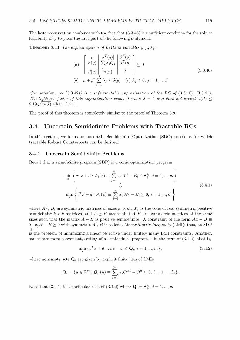
3.4. UNCERTAIN SEMIDEFINITE PROBLEMS WITH TRACTABLE RCS 119
The latter observation combines with the fact that (3.3.45) is a sufficient condition for the robustfeasibility of y to yield the first part of the following statement:
Theorem 3.11 The explicit system of LMIs in variables y, µ, λj:
(a)
µ σT (y)] βT (y)σ(y)
∑j
λjQj αT (y)
β(y) α(y) I
º 0
(b) µ + ρ2J∑
j=1λj ≤ δ(y) (c) λj ≥ 0, j = 1, ..., J
(3.3.46)
(for notation, see (3.3.42)) is a safe tractable approximation of the RC of (3.3.40), (3.3.41).The tightness factor of this approximation equals 1 when J = 1 and does not exceed Ω(J) ≤9.19
√ln(J) when J > 1.
The proof of this theorem is completely similar to the proof of Theorem 3.9.
3.4 Uncertain Semidefinite Problems with Tractable RCs
In this section, we focus on uncertain Semidefinite Optimization (SDO) problems for whichtractable Robust Counterparts can be derived.
3.4.1 Uncertain Semidefinite Problems
Recall that a semidefinite program (SDP) is a conic optimization program
minx
cT x + d : Ai(x) ≡
n∑j=1
xjAij −Bi ∈ Ski
+ , i = 1, ...,m
mmin
x
cT x + d : Ai(x) ≡
n∑j=1
xjAij −Bi º 0, i = 1, ..., m
(3.4.1)
where Aij , Bi are symmetric matrices of sizes ki × ki, Sk+ is the cone of real symmetric positive
semidefinite k × k matrices, and A º B means that A,B are symmetric matrices of the samesizes such that the matrix A − B is positive semidefinite. A constraint of the form Ax − B ≡∑j
xjAj−B º 0 with symmetric Aj , B is called a Linear Matrix Inequality (LMI); thus, an SDP
is the problem of minimizing a linear objective under finitely many LMI constraints. Another,sometimes more convenient, setting of a semidefinite program is in the form of (3.1.2), that is,
minx
cT x + d : Aix− bi ∈ Qi, i = 1, ...,m
, (3.4.2)
where nonempty sets Qi are given by explicit finite lists of LMIs:
Qi = u ∈ Rpi : Qi`(u) ≡pi∑
s=1
usQsi` −Qi` º 0, ` = 1, ..., Li.
Note that (3.4.1) is a particular case of (3.4.2) where Qi = Ski+ , i = 1, ..., m.

120 LECTURE 3: ROBUST CONIC OPTIMIZATION
The notions of the data of a semidefinite program, of an uncertain semidefinite problem andof its (exact or approximate) Robust Counterparts are readily given by specializing the generaldescriptions from sections 3.1, 3.1.4, to the case when the underlying cones are the cones ofpositive semidefinite matrices. In particular,
• The natural data of a semidefinite program (3.4.2) is the collection
(c, d, Ai, bimi=1),
while the right hand side sets Qi are treated as the problem’s structure;• An uncertain semidefinite problem is a collection of problems (3.4.2) with common structure
and natural data running through an uncertainty set; we always assume that the data areaffinely parameterized by perturbation vector ζ ∈ RL running through a given closed and convexperturbation set Z such that 0 ∈ Z:
[c; d] = [cn; dn] +L∑
`=1
ζ`[c`; d`];
[Ai, bi] = [Ani , bni ] +
L∑`=1
ζ`[A`i , b
`i ], i = 1, ..., m
(3.4.3)
• The Robust Counterpart of uncertain SDP (3.4.2), (3.4.3) at a perturbation level ρ > 0 isthe semi-infinite optimization program
miny=(x,t)
t :[[cn]T x + dn] +
L∑`=1
ζ`[[c`]T x + d`] ≤ t
[Ani x + bni ] +
L∑`=1
ζ`[A`ix + b`
i ] ∈ Qi, i = 1, ..., m
∀ζ ∈ ρZ
(3.4.4)
• A safe tractable approximation of the RC of uncertain SDP (3.4.2), (3.4.3) is a finite systemSρ of explicitly computable convex constraints in variables y = (x, t) (and possibly additionalvariables u) depending on ρ > 0 as a parameter, such that the projection Yρ of the solution setof the system onto the space of y variables is contained in the feasible set Yρ of (3.4.4). Suchan approximation is called tight within factor ϑ ≥ 1, if Yρ ⊃ Yρ ⊃ Yϑρ. In other words, Sρ is aϑ-tight safe approximation of (3.4.4), if:
1. Whenever ρ > 0 and y are such that y can be extended, by a properly chosen u, to asolution of Sρ, y is robust feasible at the uncertainty level ρ, (i.e., y is feasible for (3.4.4)).
2. Whenever ρ > 0 and y are such that y cannot be extended to a feasible solution to Sρ, yis not robust feasible at the uncertainty level ϑρ, (i.e., y violates some of the constraintsin (3.4.4) when ρ is replaced with ϑρ).
3.4.2 Tractability of RCs of Uncertain Semidefinite Problems
Building the RC of an uncertain semidefinite problem reduces to building the RCs of the uncer-tain constraints constituting the problem, so that the tractability issues in Robust SemidefiniteOptimization reduce to those for the Robust Counterpart
Aζ(y) ≡ An(y) +L∑
`=1
ζ`A`(y) º 0 ∀ζ ∈ ρZ (3.4.5)

3.4. UNCERTAIN SEMIDEFINITE PROBLEMS WITH TRACTABLE RCS 121
of a single uncertain LMI
Aζ(y) ≡ An(y) +L∑
`=1
ζ`A`(y) º 0; (3.4.6)
here An(x), A`(x) are symmetric matrices affinely depending on the design vector y.More often than not the RC of an uncertain LMI is computationally intractable. Indeed, we
saw in section 3 that intractability is typical already for the RCs of uncertain conic quadraticinequalities, and the latter are very special cases of uncertain LMIs (due to the fact that Lorentzcones are cross-sections of semidefinite cones, see Lemma 3.1). In the relatively simple case ofuncertain CQIs, we met just 3 generic cases where the RCs were computationally tractable,specifically, the cases of
1. Scenario perturbation set (section 3.2.1);
2. Unstructured norm-bounded uncertainty (section 3.2.3);
3. Simple ellipsoidal uncertainty (section 3.2.5).
The RC associated with a scenario perturbation set is tractable for an arbitrary uncertain conicproblem on a tractable cone; in particular, the RC of an uncertain LMI with scenario pertur-bation set is computationally tractable. Specifically, if Z in (3.4.5) is given as Convζ1, ..., ζN,then the RC (3.4.5) is nothing but the explicit system of LMIs
An(y) +L∑
`=1
ζi`A`(y) º 0, i = 1, ..., N. (3.4.7)
The fact that the simple ellipsoidal uncertainty (Z is an ellipsoid) results in a tractable RCis specific for Conic Quadratic Optimization. In the LMI case, (3.4.5) can be NP-hard evenwith an ellipsoid in the role of Z. In contrast to this, the case of unstructured norm-boundedperturbations remains tractable in the LMI situation. This is the only nontrivial tractable casewe know. We are about to consider this case in full details.
Unstructured Norm-Bounded Perturbations
Definition 3.5 We say that uncertain LMI (3.4.6) is with unstructured norm-bounded pertur-bations, if
1. The perturbation set Z (see (3.4.3)) is the set of all p× q matrices ζ with the usual matrixnorm ‖ · ‖2,2 not exceeding 1;
2. “The body” Aζ(y) of (3.4.6) can be represented as
Aζ(y) ≡ An(y) +[LT (y)ζR(y) + RT (y)ζT L(y)
], (3.4.8)
where both L(·), R(·) are affine and at least one of these matrix-valued functions is in factindependent of y.
Example 3.3 Consider the situation where Z is the unit Euclidean ball in RL (or, which is the same,the set of L× 1 matrices of ‖ · ‖2,2-norm not exceeding 1), and
Aζ(y) =[
a(y) ζT BT (y) + bT (y)B(y)ζ + b(y) A(y)
], (3.4.9)

122 LECTURE 3: ROBUST CONIC OPTIMIZATION
where a(·) is an affine scalar function, and b(·), B(·), A(·) are affine vector- and matrix-valued functionswith A(·) ∈ SM . Setting R(y) ≡ R = [1, 01×M ], L(y) = [0L×1, B
T (y)], we have
Aζ(y) =[
a(y) bT (y)b(y) A(y)
]
︸ ︷︷ ︸An(y)
+LT (y)ζR(y) + RT (y)ζT L(y),
thus, we are in the case of an unstructured norm-bounded uncertainty.
A closely related example is given by the LMI reformulation of an uncertain Least Squaresinequality with unstructured norm-bounded uncertainty, see section 3.2.3.
Let us derive a tractable reformulation of an uncertain LMI with unstructured norm-boundeduncertainty. W.l.o.g. we may assume that R(y) ≡ R is independent of y (otherwise we can swapζ and ζT , swapping simultaneously L and R) and that R 6= 0. We have
y is robust feasible for (3.4.6), (3.4.8) at uncertainty level ρ
⇔ ξT [An(y) + LT (y)ζR + RT ζT L(y)]ξ ≥ 0 ∀ξ ∀(ζ : ‖ζ‖2,2 ≤ ρ)
⇔ ξTAn(y)ξ + 2ξT LT (y)ζRξ ≥ 0 ∀ξ ∀(ζ : ‖ζ‖2,2 ≤ ρ)
⇔ ξTAn(y)ξ + 2min‖ζ‖2,2≤ρξT LT (y)ζRξ︸ ︷︷ ︸
=−ρ‖L(y)ξ‖2‖Rξ‖2
≥ 0 ∀ξ
⇔ ξTAn(y)ξ − 2ρ‖L(y)ξ‖2‖Rξ‖2 ≥ 0 ∀ξ⇔ ξTAn(y)ξ + 2ρηT L(y)ξ ≥ 0 ∀(ξ, η : ηT η ≤ ξT RT Rξ)
⇔ ∃λ ≥ 0 :[
ρL(y)ρLT (y) An(y)
]º λ
[ −Ip
RT R
][S-Lemma]
⇔ ∃λ :[
λIp ρL(y)ρLT (y) An(y)− λRT R
]º 0.
We have proved the following statement:
Theorem 3.12 The RC
An(y) + LT (y)ζR + RT ζT L(y) º 0 ∀(ζ ∈ Rp×q : ‖ζ‖2,2 ≤ ρ) (3.4.10)
of uncertain LMI (3.4.6) with unstructured norm-bounded uncertainty (3.4.8) (where, w.l.o.g.,we assume that R 6= 0) can be represented equivalently by the LMI
[λIp ρL(y)
ρLT (y) An(y)− λRT R
]º 0 (3.4.11)
in variables y, λ.
Application: Robust Structural Design
Structural Design problem. Consider a “linearly elastic” mechanical system S that, math-ematically, can be characterized by:
3.4. UNCERTAIN SEMIDEFINITE PROBLEMS WITH TRACTABLE RCS 123
1. A linear space RM of virtual displacements of the system.
2. A symmetric positive semidefinite M × M matrix A, called the stiffness matrix of thesystem.
The potential energy capacitated by the system when its displacement from the equilibriumis v is
E =12vT Av.
An external load applied to the system is given by a vector f ∈ RM . The associatedequilibrium displacement v of the system solves the linear equation
Av = f.
If this equation has no solutions, the load destroys the system — no equilibrium exists; if thesolution is not unique, so is the equilibrium displacement. Both these “bad phenomena” canoccur only when A is not positive definite.
The compliance of the system under a load f is the potential energy capacitated by thesystem in the equilibrium displacement v associated with f , that is,
Complf (A) =12vT Av =
12vT f.
An equivalent way to define compliance is as follows. Given external load f , consider the concavequadratic form
fT v − 12vT Av
on the space RM of virtual displacements. It is easily seen that this form either is unboundedabove, (which is the case when no equilibrium displacements exist), or attains its maximum. Inthe latter case, the compliance is nothing but the maximal value of the form:
Complf (A) = supv∈RM
[fT v − 1
2vT Av
],
and the equilibrium displacements are exactly the maximizers of the form.There are good reasons to treat the compliance as the measure of rigidity of the construction
with respect to the corresponding load — the less the compliance, the higher the rigidity. Atypical Structural Design problem is as follows:
Structural Design: Given
• the space RM of virtual displacements of the construction,
• the stiffness matrix A = A(t) affinely depending on a vector t of design param-eters restricted to reside in a given convex compact set T ⊂ RN ,
• a set F ⊂ RM of external loads,
find a construction t∗ that is as rigid as possible w.r.t. the “most dangerous” loadfrom F , that is,
t∗ ∈ ArgminT∈T
ComplF (t) ≡ sup
f∈FComplf (A(t))
.
124 LECTURE 3: ROBUST CONIC OPTIMIZATION
Next we present three examples of Structural Design.
Example 3.4 Truss Topology Design. A truss is a mechanical construction, like railroad bridge,electric mast, or the Eiffel Tower, comprised of thin elastic bars linked to each other at nodes. Some ofthe nodes are partially or completely fixed, so that their virtual displacements form proper subspacesin R2 (for planar constructions) or R3 (for spatial ones). An external load is a collection of externalforces acting at the nodes. Under such a load, the nodes move slightly, thus causing elongations andcompressions in the bars, until the construction achieves an equilibrium, where the tensions caused in thebars as a result of their deformations compensate the external forces. The compliance is the potentialenergy capacitated in the truss at the equilibrium as a result of deformations of the bars.
A mathematical model of the outlined situation is as follows.• Nodes and the space of virtual displacements. Let M be the nodal set, that is, a finite setin Rd (d = 2 for planar and d = 3 for spatial trusses), and let Vi ⊂ Rd be the linear spaceof virtual displacements of node i. (This set is the entire Rd for non-supported nodes, is 0for fixed nodes and is something in-between these two extremes for partially fixed nodes.) Thespace V = RM of virtual displacements of the truss is the direct product V = V1 × ... × Vm ofthe spaces of virtual displacements of the nodes, so that a virtual displacement of the truss is acollection of “physical” virtual displacements of the nodes.
Now, an external load applied to the truss can be thought of as a collection of externalphysical forces fi ∈ Rd acting at nodes i from the nodal set. We lose nothing when assumingthat fi ∈ Vi for all i, since the component of fi orthogonal to Vi is fully compensated by thesupports that make the directions from Vi the only possible displacements of node i. Thus, wecan always assume that fi ∈ Vi for all i, which makes it possible to identify a load with a vectorf ∈ V . Similarly, the collection of nodal reaction forces caused by elongations and compressionsof the bars can be thought of as a vector from V .• Bars and the stiffness matrix. Every bar j, j = 1, ..., N , in the truss links two nodes fromthe nodal set M. Denoting by tj the volume of the j-th bar, a simple analysis, (where oneassumes that the nodal displacements are small and neglects all terms of order of squares ofthese displacements), demonstrates that the collection of the reaction forces caused by a nodaldisplacement v ∈ V can be represented as A(t)v, where
A(t) =N∑
j=1
tjbjbTj (3.4.12)
is the stiffness matrix of the truss. Here bj ∈ V is readily given by the characteristics of thematerial of the j-th bar and the “nominal,” (i.e., in the unloaded truss), positions of the nodeslinked by this bar.
In a typical Truss Topology Design (TTD) problem, one is given a ground structure — aset M of tentative nodes along with the corresponding spaces Vi of virtual displacements andthe list J of N tentative bars, (i.e., a list of pairs of nodes that could be linked by bars), andthe characteristics of the bar’s material; these data determine, in particular, the vectors bj .The design variables are the volumes tj of the tentative bars. The design specifications alwaysinclude the natural restrictions tj ≥ 0 and an upper bound w on
∑j
tj , (which, essentially, is
an upper bound on the total weight of the truss). Thus, T is always a subset of the standardsimplex t ∈ RN : t ≥ 0,
∑j
tj ≤ w. There could be other design specifications, like upper
and lower bounds on the volumes of some bars. The scenario set F usually is either a singleton
3.4. UNCERTAIN SEMIDEFINITE PROBLEMS WITH TRACTABLE RCS 125
(single-load TTD) or a small collection of external loads (multi-load TTD). With this setup, oneseeks for a design t ∈ T , that results in the smallest possible worst case, i.e., maximal over theloads from F compliance.
When formulating a TTD problem, one usually starts with a dense nodal set and allows forall pair connections of the tentative nodes by bars. At an optimal solution to the associatedTTD problem, usually a pretty small number of bars get positive volumes, so that the solutionrecovers not only the optimal bar sizing, but also the optimal topology of the construction.
Example 3.5 Free Material Optimization. In Free Material Optimization (FMO) one seeks todesign a mechanical construction comprised of material continuously distributed over a given 2-D or 3-Ddomain Ω, and the mechanical properties of the material are allowed to vary from point to point. Theultimate goal of the design is to build a construction satisfying a number of constraints (most notably,an upper bound on the total weight) and most rigid w.r.t. loading scenarios from a given sample.
After finite element discretization, this (originally infinite-dimensional) optimization problembecomes a particular case of the aforementioned Structural Design problem where:
• the space V = RM of virtual displacements is the space of “physical displacements” ofthe vertices of the finite element cells, so that a displacement v ∈ V is a collection ofdisplacements vi ∈ Rd of the vertices (d = 2 for planar and d = 3 for spatial constructions).Same as in the TTD problem, displacements of some of the vertices can be restricted toreside in proper linear subspaces of Rd;
• external loads are collections of physical forces applied at the vertices of the finite elementcells; same as in the TTD case, these collections can be identified with vectors f ∈ V ;
• the stiffness matrix is of the form
A(t) =N∑
j=1
S∑
s=1
bjstjbTjs, (3.4.13)
where N is the number of finite element cells and tj is the stiffness tensor of the materialin the j-th cell. This tensor can be identified with a p× p symmetric positive semidefinitematrix, where p = 3 for planar constructions and p = 6 for spatial ones. The number Sand the M × p matrices bis are readily given by the geometry of the finite element cellsand the type of finite element discretization.
In a typical FMO problem, one is given the number of the finite element cells along with thematrices bij in (3.4.13), and a collection F of external loads of interest. The design vectors arecollections t = (t1, ..., tN ) of positive semidefinite p × p matrices, and the design specificationsalways include the natural restrictions tj º 0 and an upper bound
∑j
cjTr(tj) ≤ w, cj > 0,
on the total weighted trace of tj ; this bound reflects, essentially, an upper bound on the totalweight of the construction. Along with these restrictions, the description of the feasible designset T can include other constraints, such as bounds on the spectra of tj , (i.e., lower bounds onthe minimal and upper bounds on the maximal eigenvalues of tj). With this setup, one seeksfor a design t ∈ T that results in the smallest worst case, (i.e., the maximal over the loads fromF) compliance.
The design yielded by FMO usually cannot be implemented “as it is” — in most cases, itwould be either impossible, or too expensive to use a material with mechanical properties varying
126 LECTURE 3: ROBUST CONIC OPTIMIZATION
from point to point. The role of FMO is in providing an engineer with an “educated guess” ofwhat the optimal construction could possibly be; given this guess, engineers produce somethingsimilar from composite materials, applying existing design tools that take into account finerdesign specifications, (which may include nonconvex ones), than those taken into considerationby the FMO design model.
Our third example, due to C. Roos, has nothing in common with mechanics — it is aboutdesign of electrical circuits. Mathematically, however, it is modeled as a Structural Designproblem.
Example 3.6 Consider an electrical circuit comprised of resistances and sources of current. Mathe-matically, such a circuit can be thought of as a graph with nodes 1, ..., n and a set E of oriented arcs.Every arc γ is assigned with its conductance σγ ≥ 0 (so that 1/σγ is the resistance of the arc). The nodesare equipped with external sources of current, so every node i is assigned with a real number fi — thecurrent supplied by the source. The steady state functioning of the circuit is characterized by currentsγ in the arcs and potentials vi at the nodes, (these potentials are defined up to a common additiveconstant). The potentials and the currents can be found from the Kirchhoff laws, specifically, as follows.Let G be the node-arc incidence matrix, so that the columns in G are indexed by the nodes, the rows areindexed by the arcs, and Gγi is 1, −1 or 0, depending on whether the arc γ starts at node i, ends at thisnode, or is not incident to the node, respectively. The first Kirchhoff law states that sum of all currentsin the arcs leaving a given node minus the sum of all currents in the arcs entering the node is equal tothe external current at the node. Mathematically, this law reads
GT = f,
where f = (f1, ..., fn) and = γγ∈E are the vector of external currents and the vector of currents inthe arcs, respectively. The second law states that the current in an arc γ is σγ times the arc voltage —the difference of potentials at the nodes linked by the arc. Mathematically, this law reads
= ΣGv, Σ = Diagσγ , γ ∈ E.
Thus, the potentials are given by the relation
GT ΣGv = f.
Now, the heat H dissipated in the circuit is the sum, over the arcs, of the products of arc currents andarc voltages, that is,
H =∑
γ
σγ((Gv)γ)2 = vT GT ΣGv.
In other words, the heat dissipated in the circuit, the external currents forming a vector f , is the maximumof the convex quadratic form
2vT f − vT GT ΣGv
over all v ∈ Rn, and the steady state potentials are exactly the maximizers of this quadratic form. Inother words, the situation is as if we were speaking about a mechanical system with stiffness matrixA(σ) = GT ΣG affinely depending on the vector σ ≥ 0 of arc conductances subject to external load f ,with the steady-state potentials in the role of equilibrium displacements, and the dissipated heat in thisstate in the role of (twice) the compliance.
It should be noted that the “stiffness matrix” in our present situation is degenerate — indeed,we clearly have G1 = 0, where 1 is the vector of ones, (“when the potentials of all nodesare equal, the currents in the arcs should be zero”), whence A(σ)1 = 0 as well. As a result,the necessary condition for the steady state to exist is fT 1 = 0, that is, the total sum of allexternal currents should be zero — a fact we could easily foresee. Whether this necessarycondition is also sufficient depends on the topology of the circuit.

3.4. UNCERTAIN SEMIDEFINITE PROBLEMS WITH TRACTABLE RCS 127
A straightforward “electrical” analogy of the Structural Design problem would be to build a circuit ofa given topology, (i.e., to equip the arcs of a given graph with nonnegative conductances forming a designvector σ), satisfying specifications σ ∈ S in a way that minimizes the maximal steady-state dissipatedheat, the maximum being taken over a given family F of vectors of external currents.
Structural Design as an uncertain Semidefinite problem. The aforementioned Struc-tural Design problem can be easily posed as an SDP. The key element in the transformation ofthe problem is the following semidefinite representation of the compliance:
Complf (A) ≤ τ ⇔[
2τ fT
f A
]º 0. (3.4.14)
Indeed,Complf (A) ≤ τ
⇔ fT v − 12vT Av ≥ τ ∀v ∈ RM
⇔ 2τs2 − 2sfT v + vT Av ≥ 0 ∀([v, s] ∈ RM+1)
⇔[
2τ −fT
−f A
]º 0
⇔[
2τ fT
f A
]º 0
where the last ⇔ follows from the fact that[
2τ −fT
−f A
]=
[1
−I
] [2τ fT
f A
] [1
−I
]T
.
Thus, the Structural Design problem can be posed as
minτ,t
τ :
[2τ fT
f A(t)
]º 0 ∀f ∈ F , t ∈ T
. (3.4.15)
Assuming that the set T of feasible designs is LMI representable, problem (3.4.15) is nothingbut the RC of the uncertain semidefinite problem
minτ,t
τ :
[2τ fT
f A(t)
]º 0, t ∈ T
, (3.4.16)
where the only uncertain data is the load f , and this data varies in a given set F (or, which isthe same, in its closed convex hull cl Conv(F)). Thus, in fact we are speaking about the RC ofa single-load Structural Design problem, with the load in the role of uncertain data varying inthe uncertainty set U = cl Conv(F).
In actual design the set F of loads of interest is finite and usually quite small. For example,when designing a bridge for cars, an engineer is interested in a quite restricted family of scenarios,primarily in the load coming from many cars uniformly distributed along the bridge (this is,essentially, what happens in rush hours), and, perhaps, in a few other scenarios (like loadscoming from a single heavy car in various positions). With finite F = f1, ..., fk, we are in thesituation of a scenario uncertainty, and the RC of (3.4.16) is the explicit semidefinite program
minτ,t
τ :
[2τ [f i]T
f i A(t)
]º 0, i = 1, ..., k, t ∈ T
.

128 LECTURE 3: ROBUST CONIC OPTIMIZATION
Note, however, that in reality the would-be construction will be affected by small “occasional”loads (like side wind in the case of a bridge), and the construction should be stable with respectto these loads. It turns out, however, that the latter requirement is not necessarily satisfied bythe “nominal” construction that takes into consideration only the loads of primary interest. Asan instructive example, consider the design of a console.
Example 3.7 Figure 3.3.(c) represents optimal single-load design of a console with a 9× 9 nodal gridon 2-D plane; nodes from the very left column are fixed, the remaining nodes are free, and the singlescenario load is the unit force f acting down and applied at the mid-node of the very right column (seefigure 3.3.(a)). We allow nearly all tentative bars (numbering 2,039), except for (clearly redundant) barslinking fixed nodes or long bars that pass through more than two nodes and thus can be split into shorterones (figure 3.3.(b)). The set T of admissible designs is given solely by the weight restriction:
T = t ∈ R2039 : t ≥ 0,
2039∑
i=1
ti ≤ 1
(compliance is homogeneous of order 1 w.r.t. t: Complf (λt) = λComplf (t), λ > 0, so we can normalizethe weight bound to be 1).
The compliance, in an appropriate scale, of the resulting nominally optimal truss (12 nodes, 24 bars)w.r.t. the scenario load f is 1.00. At the same time, the construction turns out to be highly unstable w.r.t.small “occasional” loads distributed along the 10 free nodes used by the nominal design. For example,the mean compliance of the nominal design w.r.t. a random load h ∼ N (0, 10−9I20) is 5.406 (5.4 timeslarger than the nominal compliance), while the “typical” norm ‖h‖2 of this random load is 10−4.5
√20 —
more than three orders of magnitude less than the norm ‖f‖2 = 1 of the scenario load. The complianceof the nominally optimal truss w.r.t. a “bad” load g that is 104 times smaller than f (‖g‖2 = 10−4‖f‖2)is 27.6 — by factor 27 larger than the compliance w.r.t. f ! Figure 3.3.(e) shows the deformation of thenominal design under the load 10−4g (that is, the load that is 108 (!) times smaller than the scenarioload). One can compare this deformation with the one under the load f (figure 3.3.(d)). Figure 3.3.(f)depicts shifts of the nodes under a sample of 100 random loads h ∼ N (0, 10−16I20) — loads of norm by7 plus orders of magnitude less than ‖f‖2 = 1.
To prevent the optimal design from being crushed by a small load that is outside of the setF of loading scenarios, it makes sense to extend F to a more “massive” set, primarily by addingto F all loads of magnitude not exceeding a given “small” uncertainty level ρ. A challenge hereis to decide where the small loads can be applied. In problems like TTD, it does not make senseto require the would-be construction to be capable of carrying small loads distributed alongall nodes of the ground structure; indeed, not all of these nodes should be present in the finaldesign, and of course there is no reason to bother about forces acting at non-existing nodes. Thedifficulty is that we do not know in advance which nodes will be present in the final design. Onepossibility to resolve this difficulty to some extent is to use a two-stage procedure as follows:
• at the first stage, we seek for the “nominal” design — the one that is optimal w.r.t. the“small” set F comprised of the scenario loads and, perhaps, all loads of magnitude ≤ ρ actingalong the same nodes as the scenario loads — these nodes definitely will be present in theresulting design;
• at the second stage, we solve the problem again, with the nodes actually used by thenominal design in the role of our new nodal set M+, and extend F to the set F+ by taking theunion of F and the Euclidean ball Bρ of all loads g, ‖g‖2 ≤ ρ, acting along M+.We have arrived at the necessity to solve (3.4.15) in the situation where F is the union of afinite set f1, ..., fk and a Euclidean ball. This is a particular case of the situation when F is
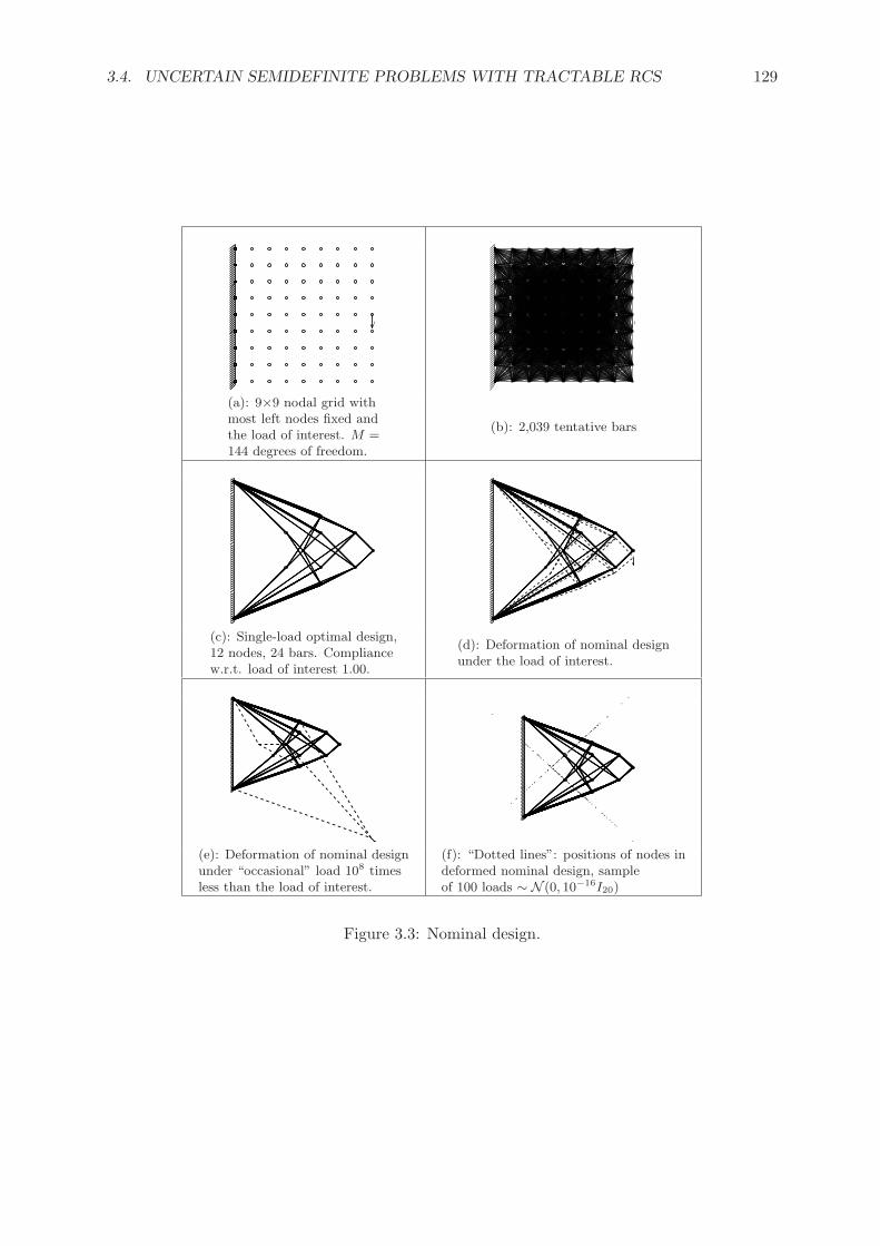
3.4. UNCERTAIN SEMIDEFINITE PROBLEMS WITH TRACTABLE RCS 129
f f
(a): 9×9 nodal grid withmost left nodes fixed andthe load of interest. M =144 degrees of freedom.
(b): 2,039 tentative bars
(c): Single-load optimal design,12 nodes, 24 bars. Compliancew.r.t. load of interest 1.00.
(d): Deformation of nominal designunder the load of interest.
(e): Deformation of nominal designunder “occasional” load 108 timesless than the load of interest.
(f): “Dotted lines”: positions of nodes indeformed nominal design, sampleof 100 loads ∼ N (0, 10−16I20)
Figure 3.3: Nominal design.

130 LECTURE 3: ROBUST CONIC OPTIMIZATION
the union of S < ∞ ellipsoids
Es = f = fs + Bsζs : ζs ∈ Rks , ‖ζs‖2 ≤ 1
or, which is the same, Z is the convex hull of the union of S ellipsoids E1, ..., ES . The associated“uncertainty-immunized” Structural Design problem (3.4.15) — the RC of (3.4.16) with Z inthe role of F — is clearly equivalent to the problem
mint,τ
τ :
[2τ fT
f A(t)
]º 0 ∀f ∈ Es, s = 1, ..., S; t ∈ T
. (3.4.17)
In order to build a tractable equivalent of this semi-infinite semidefinite problem, we need tobuild a tractable equivalent to a semi-infinite LMI of the form
[2τ ζT BT + fT
Bζ + f A(t)
]º 0 ∀(ζ ∈ Rk : ‖ζ‖2 ≤ ρ). (3.4.18)
But such an equivalent is readily given by Theorem 3.12 (cf. Example 3.3). Applying the recipedescribed in this Theorem, we end up with a representation of (3.4.18) as the following LMI invariables τ , t, λ:
λIk ρBT
2τ − λ fT
ρB f A(t)
º 0. (3.4.19)
Observe that when f = 0, (3.4.19) simplifies to[
2τIk ρBT
ρB A(t)
]º 0. (3.4.20)
Example 3.7 continued. Let us apply the outlined methodology to the Console example(Example 3.7). In order to immunize the design depicted on figure 3.3.(c) against small occa-sional loads, we start with reducing the initial 9× 9 nodal set to the set of 12 nodes M+ (figure3.4.(a)) used by the nominal design, and allow for N = 54 tentative bars on this reduced nodalset (figure 5.1.(b)) (we again allow for all pair connections of nodes, except for connections oftwo fixed nodes and for long bars passing through more than two nodes). According to theoutlined methodology, we should then extend the original singleton F = f of scenario loadsto the larger set F+ = f ∪ Bρ, where Bρ is the Euclidean ball of radius ρ, centered at theorigin in the (M = 20)-dimensional space of virtual displacements of the reduced planar nodalset. With this approach, an immediate question would be how to specify ρ. In order to avoidan ad hoc choice of ρ, we modify our approach as follows. Recalling that the compliance ofthe nominally optimal design w.r.t. the scenario load is 1.00, let us impose on our would-be“immunized” design the restriction that its worst case compliance w.r.t. the extended scenarioset Fρ = f ∪ Bρ should be at most τ∗ = 1.025, (i.e., 2.5% more than the optimal nominalcompliance), and maximize under this restriction the radius ρ. In other words, we seek for atruss of the same unit weight as the nominally optimal one with “nearly optimal” rigidity w.r.t.the scenario load f and as large as possible worst-case rigidity w.r.t. occasional loads of a givenmagnitude. The resulting problem is the semi-infinite semidefinite program
maxt,ρ
ρ :
[2τ∗ fT
f A(t)
]º 0
[2τ∗ ρhT
ρh A(t)
]º 0 ∀(h : ‖h‖2 ≤ 1)
t º 0,∑N
i=1 ti ≤ 1
.

3.4. UNCERTAIN SEMIDEFINITE PROBLEMS WITH TRACTABLE RCS 131
This semi-infinite program is equivalent to the usual semidefinite program
maxt,ρ
ρ :
[2τ∗ fT
f A(t)
]º 0
[2τ∗IM ρIM
ρIM A(t)
]º 0
t º 0,∑N
i=1 ti ≤ 1
(3.4.21)
(cf. (3.4.20)).Computation shows that for Example 3.7, the optimal value in (3.4.21) is ρ∗ = 0.362; the
robust design yielded by the optimal solution to the problem is depicted in figure 3.4.(c). Alongwith the differences in sizing of bars, note the difference in the structures of the robust and thenominal design (figure 3.5). Observe that passing from the nominal to the robust design, welose just 2.5% in the rigidity w.r.t. the scenario load and gain a dramatic improvement in thecapability to carry occasional loads. Indeed, the compliance of the robust truss w.r.t. every loadg of the magnitude ‖g‖2 = 0.36 (36% of the magnitude of the load of interest) is at most 1.025;the similar quantity for the nominal design is as large as 1.65×10⁹ ! An additional evidence ofthe dramatic advantages of the robust design as compared to the nominal one can be obtainedby comparing the pictures (d) through (f) in figure 3.3 with their counterparts in figure 3.4.
Applications in Robust Control
A major source of uncertain Semidefinite problems is Robust Control. An instructive exampleis given by Lyapunov Stability Analysis/Synthesis.
Lyapunov Stability Analysis. Consider a time-varying linear dynamical system “closed”by a linear output-based feedback:
(a) x(t) = Atx(t) + Btu(t) + Rtdt [open loop system, or plant](b) y(t) = Ctx(t) + Dtdt [output](c) u(t) = Kty(t) [output-based feedback]
⇓(d) x(t) = [At + BtKtCt]x(t) + [Rt + BtKtDt]dt [closed loop system]
(3.4.22)
where x(t) ∈ Rn, u(t) ∈ Rm, dt ∈ Rp, y(t) ∈ Rq are respectively, the state, the control, theexternal disturbance, and the output at time t, At, Bt, Rt, Ct, Dt are matrices of appropriatesizes specifying the dynamics of the system; and Kt is the feedback matrix. We assume thatthe dynamical system in question is uncertain, meaning that we do not know the dependenciesof the matrices At,...,Kt on t; all we know is that the collection Mt = (At, Bt, Ct, Dt, Rt,Kt) ofall these matrices stays all the time within a given compact uncertainty set M. For our furtherpurposes, it makes sense to think that there exists an underlying time-invariant “nominal”system corresponding to known nominal values An,...,Kn of the matrices At, ...,Kt, while theactual dynamics corresponds to the case when the matrices drift (perhaps, in a time-dependentfashion) around their nominal values.
An important desired property of a linear dynamical system is its stability — the fact thatevery state trajectory x(t) of (every realization of) the closed loop system converges to 0 ast → ∞, provided that the external disturbances dt are identically zero. For a time-invariantlinear system
x = Qnx,

132 LECTURE 3: ROBUST CONIC OPTIMIZATION
f f
(a): reduced 12-node set withmost left nodes fixed and theload of interest. M = 20degrees of freedom.
(b): 54 tentative bars
(c): Robust optimal design, 12nodes, 24 bars. Compliancew.r.t. load of interest 1.025.
(d): Deformation of robust designunder the load of interest.
(e): Deformation of robust designunder “occasional” load 10 timesless than the load of interest.
(f): “Bold dots”: positions of nodesin deformated robust design over100 loads ∼ N (0, 10−2I20)
Figure 3.4: Robust design.

3.4. UNCERTAIN SEMIDEFINITE PROBLEMS WITH TRACTABLE RCS 133
Figure 3.5: Nominal (left) and robust (right) designs.
the necessary and sufficient stability condition is that all eigenvalues of A have negative realparts or, equivalently, that there exists a Lyapunov Stability Certificate (LSC) — a positivedefinite symmetric matrix X such that
[Qn]T X + XQn ≺ 0.
For uncertain system (3.4.22), a sufficient stability condition is that all matrices
Q ∈ Q = Q = AM + BMKMCM : M ∈Mhave a common LSC X, that is, there exists X Â 0 such that
(a) QT X + XQT ≺ 0 ∀Q ∈ Qm
(b) [AM + BMKMCM ]T X + X[AM + BMKMCM ] ≺ 0 ∀M ∈M;(3.4.23)
here AM ,...,KM are the components of a collection M ∈M.
The fact that the existence of a common LSC for all matrices Q ∈ Q is sufficient for thestability of the closed loop system is nearly evident. Indeed, since M is compact, for everyfeasible solution X Â 0 of the semi-infinite LMI (3.4.23) one has
∀M ∈M : [AM + BMKMCM ]T X + X[AM + BMKMCM ] ≺ −αX (∗)with appropriate α > 0. Now let us look what happens with the quadratic form xT Xx alonga state trajectory x(t) of (3.4.22). Setting f(t) = xT (t)Xx(t) and invoking (3.4.22.d), wehave
f ′(t) = xT (t)Xx(t) + x(t)Xx(t)= xT (t)
[[At + BtKtCt]T X + X[At + BtKtCt]
]x(t)
≤ −αf(t),
where the concluding inequality is due to (∗). From the resulting differential inequality
f ′(t) ≤ −αf(t)
it follows thatf(t) ≤ exp−αtf(0) → 0, t →∞.
Recalling that f(t) = xT (t)Xx(t) and X is positive definite, we conclude that x(t) → 0 ast →∞.

134 LECTURE 3: ROBUST CONIC OPTIMIZATION
Observe that the set Q is compact along with M. It follows that X is an LSC if and only ifX Â 0 and
∃β > 0 : QT X + XQ ¹ −βI ∀Q ∈ Q⇔ ∃β > 0 : QT X + XQ ¹ −βI ∀Q ∈ Conv(Q).
Multiplying such an X by an appropriate positive real, we can ensure that
X º I & QT X + XQ ¹ −I ∀Q ∈ Conv(Q). (3.4.24)
Thus, we lose nothing when requiring from an LSC to satisfy the latter system of (semi-infinite)LMIs, and from now on LSCs in question will be exactly the solutions of this system.
Observe that (3.4.24) is nothing but the RC of the uncertain system of LMIs
X º I & QT X + XQ ¹ −I, (3.4.25)
the uncertain data being Q and the uncertainty set being Conv(Q). Thus, RCs arise naturallyin the context of Robust Control.
Now let us apply the results on tractability of the RCs of uncertain LMI in order to under-stand when the question of existence of an LSC for a given uncertain system (3.4.22) can beposed in a computationally tractable form. There are, essentially, two such cases — polytopicand unstructured norm-bounded uncertainty.Polytopic uncertainty. By definition, polytopic uncertainty means that the set Conv(Q) isgiven as a convex hull of an explicit list of “scenarios” Qi, i = 1, ..., N :
Conv(Q) = ConvQ1, ..., QN.In our context this situation occurs when the components AM , BM , CM , KM of M ∈ M run,independently of each other, through convex hulls of respective scenarios
SA = ConvA1, ..., ANA, SB = ConvB1, ..., BNB,SC = ConvC1, ..., CNC, SK = ConvK1, ..., KNK;
in this case, the set Conv(Q) is nothing but the convex hull of N = NANBNCNK “scenarios”Qijk` = Ai + BjK`Ck, 1 ≤ i ≤ NA,...,1 ≤ ` ≤ NK .
Indeed, Q clearly contains all matrices Qijk` and therefore Conv(Q) ⊃ Conv(Qijk`). Onthe other hand, the mapping (A,B,C, K) 7→ A+BKC is polylinear, so that the image Q ofthe set SA×SB×SC×SK under this mapping is contained in the convex set Conv(Qijk`),whence Conv(Qijk`) ⊃ Conv(Q).
In the case in question we are in the situation of scenario perturbations, so that (3.4.25) isequivalent to the explicit system of LMIs
X º I, [Qi]T X + XQi ¹ −I, i = 1, ..., N.
Unstructured norm-bounded uncertainty. Here
Conv(Q) = Q = Qn + UζV : ζ ∈ Rp×q, ‖ζ‖2,2 ≤ ρ.In our context this situation occurs, e.g., when 3 of the 4 matrices AM , BM , CM , KM , M ∈M, are in fact certain, and the remaining matrix, say, AM , runs through a set of the formAn + GζH : ζ ∈ Rp×q, ‖ζ‖2,2 ≤ ρ.

3.4. UNCERTAIN SEMIDEFINITE PROBLEMS WITH TRACTABLE RCS 135
In the case of unstructured norm-bounded uncertainty, the semi-infinite LMI in (3.4.25) isof the form
QT X + XQ ¹ −I ∀Q ∈ Conv(Q)m
−I − [Qn]T X −XQn︸ ︷︷ ︸
An(X)
+[−XU︸ ︷︷ ︸LT (X)
ζ V︸︷︷︸R
+RT ζT L(X)] º 0
∀(ζ ∈ Rp×q, ‖ζ‖2,2 ≤ ρ).
Invoking Theorem 3.12, (3.4.25) is equivalent to the explicit system of LMIs
X º I,
[λIp ρUT X
ρXU −I − [Qn]T X −XQn − λV T V
]º 0. (3.4.26)
in variables X,λ.
Lyapunov Stability Synthesis. We have considered the Stability Analysis problem, whereone, given an uncertain closed-loop dynamical system along with the associated uncertaintyset M, seeks to verify a sufficient stability condition. A more challenging problem is StabilitySynthesis: given an uncertain open loop system (3.4.22.a–b) along with the associated compactuncertainty set M in the space of collections M = (A,B, C,D, R), find a linear output-basedfeedback
u(t) = Ky(t)
and an LSC for the resulting closed loop system.The Synthesis problem has a nice solution, due to [22], in the case of state-based feedback
(that is, Ct ≡ I) and under the assumption that the feedback is implemented exactly, so thatthe state dynamics of the closed loop system is given by
x(t) = [At + BtK]x(t) + [Rt + BtKDt]dt. (3.4.27)
The pairs (K, X) of “feedback – LSC” that we are looking for are exactly the feasible solutionsto the system of semi-infinite matrix inequalities in variables X,K:
X Â 0 & [A + BK]T X + X[A + BK] ≺ 0 ∀[A, B] ∈ AB; (3.4.28)
here AB is the projection of M on the space of [A,B] data. The difficulty is that the system isnonlinear in the variables. As a remedy, let us carry out the nonlinear substitution of variablesX = Y −1, K = ZY −1. With this substitution, (3.4.28) becomes a system in the new variablesY, Z:
Y Â 0 & [A + BZY −1]T Y −1 + Y −1[A + BZY −1] ≺ 0 ∀[A,B] ∈ AB;
multiplying both sides of the second matrix inequality from the left and from the right by Y ,we convert the system to the equivalent form
Y Â 0, & AY + Y AT + BZ + ZT BT ≺ 0 ∀[A,B] ∈ AB.
Since AB is compact along with M, the solutions to the latter system are exactly the pairs(Y, Z) that can be obtained by scaling (Y, Z) 7→ (λY, λZ), λ > 0, from the solutions to thesystem of semi-infinite LMIs
Y º I & AY + Y AT + BZ + ZT BT ¹ −I ∀[A,B] ∈ AB (3.4.29)
in variables Y, Z. When the uncertainty AB can be represented either as a polytopic, or asunstructured norm-bounded, the system (3.4.29) of semi-infinite LMIs admits an equivalenttractable reformulation.
136 LECTURE 3: ROBUST CONIC OPTIMIZATION
3.5 Approximating RCs of Uncertain SemidefiniteProblems
3.5.1 Tight Tractable Approximations of RCs of Uncertain SDPs with Struc-tured Norm-Bounded Uncertainty
We have seen that the possibility to reformulate the RC of an uncertain semidefinite programin a computationally tractable form is a “rare commodity,” so that there are all reasons tobe interested in the second best thing — in situations where the RC admits a tight tractableapproximation. To the best of our knowledge, just one such case is known — the case ofstructured norm-bounded uncertainty we are about to consider in this section.
Uncertain LMI with Structured Norm-Bounded Perturbations
Consider an uncertain LMIAζ(y) º 0 (3.4.6)
where the “body” Aζ(y) is bi-linear in the design vector y and the perturbation vector ζ. Thedefinition of a structured norm-bounded perturbation follows the path we got acquainted within section 3:
Definition 3.6 We say that the uncertain constraint (3.4.6) is affected by structured norm-bo-unded uncertainty with uncertainty level ρ, if
1. The perturbation set Zρ is of the form
Zρ =
ζ = (ζ1, ..., ζL) :ζ` ∈ R, |ζ`| ≤ ρ, ` ∈ Is
ζ` ∈ Rp`×q` : ‖ζ`‖2,2 ≤ ρ, ` 6∈ Is
(3.5.1)
2. The body Aζ(y) of the constraint can be represented as
Aζ(y) = An(y) +∑
`∈IS
ζ`A`(y)
+∑
` 6∈Is
[LT
` (y)ζ`R` + RT` [ζ`]T L`(y)
],
(3.5.2)
where A`(y), ` ∈ Is, and L`(y), ` 6∈ Is, are affine in y, and R`, ` 6∈ Is, are nonzero.
Theorem 3.13 Given uncertain LMI (3.4.6) with structured norm-bounded uncertainty (3.5.1),(3.5.2), let us associate with it the following system of LMIs in variables Y`, ` = 1, ..., L, λ`,` 6∈ Is, y:
(a) Y` º ±A`(y), ` ∈ Is
(b)[
λ`Ip`L`(y)
LT` (y) Y` − λ`R
T` R`
]º 0, ` 6∈ Is
(c) An(y)− ρL∑
`=1
Y` º 0
(3.5.3)
Then system (3.5.3) is a safe tractable approximation of the RC
Aζ(y) º 0 ∀ζ ∈ Zρ (3.5.4)

3.5. APPROXIMATING RCS OF UNCERTAIN SEMIDEFINITE PROBLEMS 137
of (3.4.6), (3.5.1), (3.5.2), and the tightness factor of this approximation does not exceed ϑ(µ),where µ is the smallest integer ≥ 2 such that µ ≥ max
yRank(A`(y)) for all ` ∈ Is, and ϑ(·) is a
universal function of µ such that
ϑ(2) =π
2, ϑ(4) = 2, ϑ(µ) ≤ π
√µ/2, µ > 2.
The approximation is exact, if either L = 1, or all perturbations are scalar, (i.e., Is = 1, ..., L)and all A`(y) are of ranks not exceeding 1.
Proof. Let us fix y and observe that a collection y, Y1, ..., YL can be extended to a feasiblesolution of (3.5.3) if and only if
∀ζ ∈ Zρ :
−ρY` ¹ ζ`A`(y), ` ∈ Is,
−ρY` ¹ LT` (y)ζ`R` + RT
` [ζ`]T L`(y), ` 6∈ Is
(see Theorem 3.12). It follows that if, in addition, Y` satisfy (3.5.3.c), then y is feasible for (3.5.4),so that (3.5.3) is a safe tractable approximation of (3.5.4). The fact that this approximation istight within the factor ϑ(µ) is readily given by the real case Matrix Cube Theorem (TheoremA.7). The fact that the approximation is exact when L = 1 is evident when Is = 1 and isreadily given by Theorem 3.12 when Is = ∅. The fact that the approximation is exact when allperturbations are scalar and all matrices A`(y) are of ranks not exceeding 1 is evident. ¤
Application: Lyapunov Stability Analysis/Synthesis Revisited
We start with the Analysis problem. Consider the uncertain time-varying dynamical system(3.4.22) and assume that the uncertainty set Conv(Q) = Conv(AM +BMKMCM : M ∈M)in (3.4.24) is an interval uncertainty, meaning that
Conv(Q) = Qn + ρZ, Z = L∑
`=1
ζ`U` : ‖ζ‖∞ ≤ 1,Rank(U`) ≤ µ, 1 ≤ ` ≤ L.
(3.5.5)
Such a situation (with µ = 1) arises, e.g., when two of the 3 matrices Bt, Ct,Kt are certain,and the remaining one of these 3 matrices, say, Kt, and the matrix At are affected byentry-wise uncertainty:
(AM ,KM ) : M ∈M =
(A,K) :|Aij −An
ij | ≤ ραij∀(i, j)|Kpq −Kn
pq| ≤ ρκpq ∀(p, q)
,
In this case, denoting by Bn, Cn the (certain!) matrices Bt, Ct, we clearly have
Conv(Q) = An + BnKnCn︸ ︷︷ ︸
Qn+ρ
[ ∑i,j
ξij [αijeieTj ]
+∑p,q
ηpq[κpqBnfpg
Tq Cn]
]: |ξij | ≤ 1, |ηpq| ≤ 1
,
where ei, fp, gq are the standard basic orths in the spaces Rdim x, Rdim u and Rdim y, respec-tively. Note that the matrix coefficients at the “elementary perturbations” ξij , ηpq are ofrank 1, and these perturbations, independently of each other, run through [−1, 1] — exactlyas required in (3.5.5) for µ = 1.

138 LECTURE 3: ROBUST CONIC OPTIMIZATION
In the situation of (3.5.5), the semi-infinite Lyapunov LMI
QT X + XQ ¹ −I ∀Q ∈ Conv(Q)
in (3.4.24) reads
−I − [Qn]T X −XQn︸ ︷︷ ︸
An(X)
+ρL∑
`=1
ζ` [−UT` X −XU`]︸ ︷︷ ︸A`(X)
º 0 ∀(ζ : |ζ`| ≤ 1, ` = 1, ..., L).
(3.5.6)
We are in the case of structured norm-bounded perturbations with Is = 1, ..., L. Noting thatthe ranks of all matrices A`(X) never exceed 2µ (since all U` are of ranks ≤ µ), the safe tractableapproximation of (3.5.6) given by Theorem 3.13 is tight within the factor ϑ(2µ). It follows, inparticular, that in the case of (3.5.5) with µ = 1, we can find efficiently a lower bound, tightwithin the factor π/2, on the Lyapunov Stability Radius of the uncertain system (3.4.22) (thatis, on the supremum of those ρ for which the stability of our uncertain dynamical system canbe certified by an LSC). The lower bound in question is the supremum of those ρ for which theapproximation is feasible, and this supremum can be easily approximated to whatever accuracyby bisection.
We can process in the same fashion the Lyapunov Stability Synthesis problem in thepresence of interval uncertainty. Specifically, assume that Ct ≡ I and the uncertainty setAB = [AM , BM ] : M ∈M underlying the Synthesis problem is an interval uncertainty:
AB = [An, Bn] + ρL∑
`=1
ζ`U` : ‖ζ‖∞ ≤ 1, Rank(U`) ≤ µ∀`. (3.5.7)
We arrive at the situation of (3.5.7) with µ = 1, e.g., when AB corresponds to entry-wiseuncertainty:
AB = [An, Bn] + ρH ≡ [δA, δB] : |Hij | ≤ hij ∀i, j.
In the case of (3.5.7) the semi-infinite LMI in (3.4.29) reads
−I − [An, Bn][Y ; Z]− [Y ; Z]T [An, Bn]T︸ ︷︷ ︸An(Y,Z)
+ρL∑
`=1
ζ` [−U`[Y ;Z]− [Y ; Z]T UT` ]︸ ︷︷ ︸
A`(Y,Z)
º 0∀(ζ : |ζ`| ≤ 1, ` = 1, ..., L).(3.5.8)
We again reach a situation of structured norm-bounded uncertainty with Is = 1, ..., L and allmatrices A`(·), ` = 1, ..., L, being of ranks at most 2µ. Thus, Theorem 3.13 provides us witha tight, within factor ϑ(2µ), safe tractable approximation of the Lyapunov Stability Synthesisproblem.Illustration: Controlling a multiple pendulum. Consider a multiple pendulum (“a train”)depicted in figure 3.6. Denoting by mi, i = 1, ..., 4, the masses of the “engine” (i = 1) and the“cars” (i = 2, 3, 4, counting from right to left), Newton’s laws for the dynamical system inquestion read
m1d2
dt2x1(t) = −κ1x1(t) +κ1x2(t) +u(t)
m2d2
dt2x2(t) = κ1x1(t) −(κ1 + κ2)x2(t) +κ2x3(t)
m3d2
dt2x3(t) = κ2x2(t) −(κ2 + κ3)x3(t) +κ3x4(t)
m4d2
dt2x4(t) = κ3x3(t) −κ3x4(t),
(3.5.9)
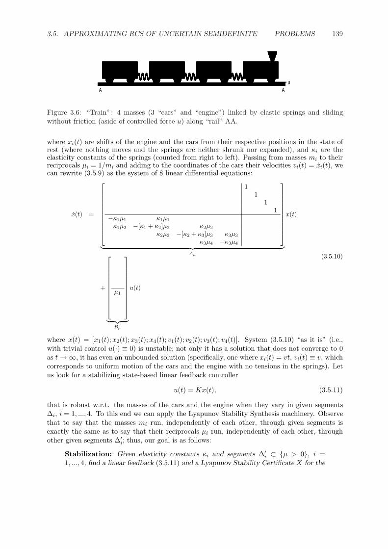
3.5. APPROXIMATING RCS OF UNCERTAIN SEMIDEFINITE PROBLEMS 139
uA A
Figure 3.6: “Train”: 4 masses (3 “cars” and “engine”) linked by elastic springs and slidingwithout friction (aside of controlled force u) along “rail” AA.
where xi(t) are shifts of the engine and the cars from their respective positions in the state ofrest (where nothing moves and the springs are neither shrunk nor expanded), and κi are theelasticity constants of the springs (counted from right to left). Passing from masses mi to theirreciprocals µi = 1/mi and adding to the coordinates of the cars their velocities vi(t) = xi(t), wecan rewrite (3.5.9) as the system of 8 linear differential equations:
x(t) =
11
11
−κ1µ1 κ1µ1
κ1µ2 −[κ1 + κ2]µ2 κ2µ2
κ2µ3 −[κ2 + κ3]µ3 κ3µ3
κ3µ4 −κ3µ4
︸ ︷︷ ︸Aµ
x(t)
+
µ1
︸ ︷︷ ︸Bµ
u(t)
(3.5.10)
where x(t) = [x1(t);x2(t);x3(t);x4(t); v1(t); v2(t); v3(t); v4(t)]. System (3.5.10) “as it is” (i.e.,with trivial control u(·) ≡ 0) is unstable; not only it has a solution that does not converge to 0as t →∞, it has even an unbounded solution (specifically, one where xi(t) = vt, vi(t) ≡ v, whichcorresponds to uniform motion of the cars and the engine with no tensions in the springs). Letus look for a stabilizing state-based linear feedback controller
u(t) = Kx(t), (3.5.11)
that is robust w.r.t. the masses of the cars and the engine when they vary in given segments∆i, i = 1, ..., 4. To this end we can apply the Lyapunov Stability Synthesis machinery. Observethat to say that the masses mi run, independently of each other, through given segments isexactly the same as to say that their reciprocals µi run, independently of each other, throughother given segments ∆′
i; thus, our goal is as follows:
Stabilization: Given elasticity constants κi and segments ∆′i ⊂ µ > 0, i =
1, ..., 4, find a linear feedback (3.5.11) and a Lyapunov Stability Certificate X for the

140 LECTURE 3: ROBUST CONIC OPTIMIZATION
corresponding closed loop system (3.5.10), (3.5.11), with the uncertainty set for thesystem being
AB = [Aµ, Bµ] : µi ∈ ∆′i, i = 1, ..., 4.
Note that in our context the Lyapunov Stability Synthesis approach is, so to speak, “doublyconservative.” First, the existence of a common LSC for all matrices Q from a given compactset Q is only a sufficient condition for the stability of the uncertain dynamical system
x(t) = Qtx(t), Qt ∈ Q∀t,and as such this condition is conservative. Second, in our train example there are reasonsto think of mi as of uncertain data (in reality the loads of the cars and the mass of theengine could vary from trip to trip, and we would not like to re-adjust the controller as longas these changes are within a reasonable range), but there is absolutely no reason to thinkof these masses as varying in time. Indeed, we could perhaps imagine a mechanism thatmakes the masses mi time-dependent, but with this mechanism our original model (3.5.9)becomes invalid — Newton’s laws in the form of (3.5.9) are not applicable to systems withvarying masses and at the very best they offer a reasonable approximation of the true model,provided that the changes in masses are slow. Thus, in our train example a common LSC forall matrices Q = A + BK, [A,B] ∈ AB, would guarantee much more than required, namely,that all trajectories of the closed loop system “train plus feedback controller” converge to 0as t →∞ even in the case when the parameters µi ∈ ∆′
i vary in time at a high speed. Thisis much more than what we actually need — convergence to 0 of all trajectories in the casewhen µi ∈ ∆′
i do not vary in time.
The system of semi-infinite LMIs we are about to process in the connection of the LyapunovStability Synthesis is
(a) [A, B][Y ; Z] + [Y ; Z]T [A, B]T ¹ −αY, ∀[A,B] ∈ AB(b) Y º I(c) Y ≤ χI,
(3.5.12)
where α > 0 and χ > 1 are given. This system differs slightly from the “canonical” system(3.4.29), and the difference is twofold:
• [major] in (3.4.29), the semi-infinite Lyapunov LMI is written as
[A,B][Y ; Z] + [Y ;Z]T [A,B]T ¹ −I,
which is just a convenient way to express the relation
[A,B][Y ; Z] + [Y ; Z]T [A,B]T ≺ 0, ∀[A,B] ∈ AB.
Every feasible solution [Y ; Z] to this LMI with Y Â 0 produces a stabilizing feedbackK = ZY −1 and the common LSC X = Y −1 for all instances of the matrix Q = A + BK,[A, B] ∈ AB, of the closed loop system, i.e.,
[A + BK]T X + X[A + BK] ≺ 0 ∀[A,B] ∈ AB.
The latter condition, however, says nothing about the corresponding decay rate. In con-trast, when [Y ; Z] is feasible for (3.5.12.a, b), the associated stabilizing feedback K = ZY −1
and LSC X = Y −1 satisfy the relation
[A + BK]T X + X[A + BK] ≺ −αX ∀[A,B] ∈ AB,
3.5. APPROXIMATING RCS OF UNCERTAIN SEMIDEFINITE PROBLEMS 141
and this relation, as we have seen when introducing the Lyapunov Stability Certificate,implies that
xT (t)Xx(t) ≤ exp−αtxT (0)Xx(0), t ≥ 0,
which guarantees that the decay rate in the closed loop system is at least α. In our illus-tration (same as in real life), we prefer to deal with this “stronger” form of the LyapunovStability Synthesis requirement, in order to have a control over the decay rate associatedwith the would-be controller.
• [minor] In (3.5.12) we impose an upper bound on the condition number (ratio of themaximal and minimal eigenvalues) of the would-be LSC; with normalization of Y given by(3.5.12.b), this bound is ensured by (3.5.12.c) and is precisely χ. The only purpose of thisbound is to avoid working with extremely ill-conditioned positive definite matrices, whichcan cause numerical problems.
Now let us use Theorem 3.13 to get a tight safe tractable approximation of the semi-infinitesystem of LMIs (3.5.12). Denoting by µn
i the midpoints of the segments ∆′i and by δi the
half-width of these segments, we have
AB ≡ [Aµ, Bµ] : µi ∈ ∆′i, i = 1, ..., 4
= [Aµn , Bµn] +4∑
`=1
ζ`U` : |ζ`| ≤ 1, ` = 1, ..., 4,U` = δ`p`q
T` ,
where p` ∈ R8 has the only nonzero entry, equal to 1, in the position 4 + `, and
qT1
qT2
qT3
qT4
=
−κ1 κ1 1κ1 −[κ1 + κ2] κ2
κ2 −[κ2 + κ3] κ3
κ3 −κ3
Consequently, the analogy of (3.5.12) with uncertainty level ρ ((3.5.12) itself corresponds toρ = 1) is the semi-infinite system of LMIs
−αY − [Aµn , Bµn][Y ; Z]− [Y ; Z]T [Aµn , Bµn]T︸ ︷︷ ︸An(Y,Z)
+ρ4∑
`=1
ζ`(−δ`[p`qT` [Y ; Z] + [Y ; Z]T q`p
T` ]︸ ︷︷ ︸
A`(Y,Z)
) º 0∀(ζ : |ζ`| ≤ 1, ` = 1, ..., 4)
Y º I8, Y ¹ χI8
(3.5.13)
in variables Y , Z (cf. (3.5.8)). The safe tractable approximation of this semi-infinite system ofLMIs as given by Theorem 3.13 is the system of LMIs
Y` º ±A`(Y, Z), ` = 1, ..., 4
An(Y, Z)− ρ4∑
`=1
Y` º 0
Y º I8, Y ¹ χI8
(3.5.14)
in variables Y, Z, Y1, ..., Y4. Since all U` are of rank 1 and therefore all A`(Y, Z) are of rank ≤ 2,Theorem 3.13 states that this safe approximation is tight within the factor π/2.

142 LECTURE 3: ROBUST CONIC OPTIMIZATION
Of course, in our toy example no approximation is needed — the set AB is a polytopicuncertainty with just 24 = 16 vertices, and we can straightforwardly convert (3.5.13) into anexactly equivalent system of 18 LMIs
An(Y, Z) º ρ4∑
`=1
ε`A`(Y, Z), ε` = ±1, ` = 1, ..., 4
Y º I8, Y ¹ χI8
in variables Y,Z. The situation would change dramatically if there were, say, 30 cars in ourtrain rather than just 3. Indeed, in the latter case the precise “polytopic” approach wouldrequire solving a system of 231 + 2 = 2, 147, 483, 650 LMIs of the size 62 × 62 in variablesY ∈ S62, Z ∈ R1×63, which is a bit too much... In contrast, the approximation (3.5.14) isa system of just 31 + 2 = 33 LMIs of the size 62 × 62 in variables Y` ∈ S6231`=1, Y ∈ S62,Z ∈ R1×63 (totally (31 + 1) 62·63
2 + 63 = 60606 scalar decision variables). One can arguethat the latter problem still is too large from a practical perspective. But in fact it can beshown that in this problem, one can easily eliminate the matrices Y` (every one of them canbe replaced with a single scalar decision variable, cf. Antenna example on p. 106), whichreduces the design dimension of the approximation to 31 + 62·63
2 + 63 = 2047. A convexproblem of this size can be solved pretty routinely.
We are about to present numerical results related to stabilization of our toy 3-car train. Thesetup in our computations is as follows:
κ1 = κ2 = κ3 = 100.0;α = 0.01;χ = 108;∆′
1 = [0.5, 1.5], ∆′2 = ∆′
3 = ∆′4 = [1.5, 4.5],
which corresponds to the mass of the engine varying in [2/3, 2] and the masses of the cars varyingin [2/9, 2/3].
We computed, by a kind of bisection, the largest ρ for which the approximation (3.5.14) isfeasible; the optimal feedback we have found is
u = 107[− 0.2892x1 − 2.5115x2 + 6.3622x3 − 3.5621x4
−0.0019v1 − 0.0912v2 − 0.0428v3 + 0.1305v4
],
and the (lower bound on the) Lyapunov Stability radius of the closed loop system as yieldedby our approximation is ρ = 1.05473. This bound is > 1, meaning that our feedback stabilizesthe train in the above ranges of the masses of the engine and the cars (and in fact, even inslightly larger ranges 0.65 ≤ m1 ≤ 2.11, 0.22 ≤ m2,m3,m4 ≤ 0.71). An interesting questionis by how much the lower bound ρ is less than the Lyapunov Stability radius ρ∗ of the closedloop system. Theory guarantees that the ratio ρ∗/ρ should be ≤ π/2 = 1.570.... In our smallproblem we can compute ρ∗ by applying the polytopic uncertainty approach, that results inρ∗ = 1.05624. Thus, in reality ρ∗/ρ ≈ 1.0014, much better than the theoretical bound 1.570....In figure 3.7, we present sample trajectories of the closed loop system yielded by our design, thelevel of perturbations being 1.054 — pretty close to ρ = 1.05473.
3.6 Approximating Chance Constrained CQIs and LMIs
In the first reading this section can be skipped.Below we develop safe tractable approximations of chance constrained randomly perturbed ConicQuadratic and Linear Matrix Inequalities. For omitted proofs, see [3].

3.6. APPROXIMATING CHANCE CONSTRAINED CQIS AND LMIS 143
0 10 20 30 40 50 60 70 80 90 100−0.5
0
0.5
1
1.5
2
2.5
0 10 20 30 40 50 60 70 80 90 100−0.5
0
0.5
1
1.5
2
coordinates x1, x2, x3, x4 velocities v1, v2, v3, v4
time horizon: 0 ≤ t ≤ 100
0 0.05 0.1 0.15 0.2 0.25 0.3 0.35 0.4 0.45 0.5−0.1
0
0.1
0.2
0.3
0.4
0.5
0.6
0 0.05 0.1 0.15 0.2 0.25 0.3 0.35 0.4 0.45 0.5−2
−1.5
−1
−0.5
0
0.5
1
1.5
2
coordinates x1, x2, x3, x4 velocities v1, v2, v3, v4
time horizon: 0 ≤ t ≤ 0.5
Figure 3.7: Sample trajectories of the 3-car train.
3.6.1 Chance Constrained LMIs
We have considered the Robust of uncertain conic quadratic and semidefinite programs. Now we intendto consider randomly perturbed CQPs and SDPs and to derive safe approximations of their chanceconstrained versions (cf. section 2.1). From this perspective, it is convenient to treat chance constrainedCQPs as particular cases of chance constrained SDPs (such an option is given by Lemma 3.1), so thatin the sequel we focus on chance constrained SDPs. Thus, we are interested in a randomly perturbedsemidefinite program
miny
cT y : An(y) + ρ
L∑
`=1
ζ`A`(y) º 0, y ∈ Y
, (3.6.1)
where An(y) and all A`(y) are affine in y, ρ ≥ 0 is the “perturbation level,” ζ = [ζ1; ...; ζL] is a randomperturbation, and Y is a semidefinite representable set. We associate with this problem its chanceconstrained version
miny
cT y : Prob
An(y) + ρ
L∑
`=1
ζ`A`(y) º 0
≥ 1− ε, y ∈ Y
(3.6.2)

144 LECTURE 3: ROBUST CONIC OPTIMIZATION
where ε ¿ 1 is a given positive tolerance. Our goal is to build a computationally tractable safe ap-proximation of (3.6.2). We start with assumptions on the random variables ζ`, which will be in forceeverywhere in the following:
Random variables ζ`, ` = 1, ..., L, are independent with zero mean satisfying eitherA.I [“bounded case”] |ζ`| ≤ 1, ` = 1, ..., L,orA.II [“Gaussian case”] ζ` ∼ N (0, 1), ` = 1, ..., L.
Note that most of the results to follow can be extended to the case when ζ` are independent with zeromeans and “light tail” distributions. We prefer to require more in order to avoid too many technicalities.
Approximating Chance Constrained LMIs: Preliminaries
The problem we are facing is basically as follows:
(?) Given symmetric matrices A,A1,...,AL, find a verifiable sufficient condition for the rela-tion
ProbL∑
`=1
ζ`A` ¹ A ≥ 1− ε. (3.6.3)
Since ζ is with zero mean, it is natural to require A º 0 (this condition clearly is necessary when ζ issymmetrically distributed w.r.t. 0 and ε < 0.5). Requiring a bit more, namely, A Â 0, we can reduce thesituation to the case when A = I, due to
ProbL∑
`=1
ζ`A` ¹ A = ProbL∑
`=1
ζ` A−1/2A`A−1/2
︸ ︷︷ ︸B`
¹ I. (3.6.4)
Now let us try to guess a verifiable sufficient condition for the relation
ProbL∑
`=1
ζ`B` ¹ I ≥ 1− ε. (3.6.5)
First of all, we do not lose much when strengthening the latter relation to
Prob‖L∑
`=1
ζ`B`‖ ≤ 1 ≥ 1− ε (3.6.6)
(here and in what follows, ‖ · ‖ stands for the standard matrix norm ‖ · ‖2,2). Indeed, the latter conditionis nothing but
Prob−I ¹L∑
`=1
ζ`B` ¹ I ≥ 1− ε,
so that it implies (3.6.5). In the case of ζ symmetrically distributed w.r.t. the origin, we have a “nearlyinverse” statement: the validity of (3.6.5) implies the validity of (3.6.6) with ε increased to 2ε.
The central observation is that whenever (3.6.6) holds true and the distribution of the random matrix
S =L∑
`=1
ζ`B`
is not pathological, we should haveE‖S2‖ ≤ O(1),
whence, by Jensen’s Inequality,‖ES2‖ ≤ O(1)

3.6. APPROXIMATING CHANCE CONSTRAINED CQIS AND LMIS 145
as well. Taking into account that ES2 =L∑
`=1
Eζ2` B2
` , we conclude that when all quantities Eζ2` are
of order of 1, we should have ‖∑L`=1 B2
` ‖ ≤ O(1), or, which is the same,
L∑
`=1
B2` ¹ O(1)I. (3.6.7)
By the above reasoning, (3.6.7) is a kind of a necessary condition for the validity of the chance constraint(3.6.6), at least for random variables ζ` that are symmetrically distributed w.r.t. the origin and are “oforder of 1.” To some extent, this condition can be treated as nearly sufficient, as is shown by the followingtwo theorems.
Theorem 3.14 Let B1, ..., BL ∈ Sm be deterministic matrices such that
L∑
`=1
B2` ¹ I (3.6.8)
and Υ > 0 be a deterministic real. Let, further, ζ`, ` = 1, ..., L, be independent random variables takingvalues in [−1, 1] such that
χ ≡ Prob
‖
L∑
`=1
ζ`B`‖ ≤ Υ
> 0. (3.6.9)
Then
∀Ω > Υ : Prob
‖
L∑
`=1
ζ`B`‖ > Ω
≤ 1
χexp−(Ω−Υ)2/16. (3.6.10)
Proof. Let Q = z ∈ RL : ‖∑`
z`B`‖ ≤ 1. Observe that
‖[∑
`
z`B`]u‖2 ≤∑
`
|z`|‖B`u‖2 ≤(∑
`
z2`
)1/2 (∑
`
uT B2` u
)1/2
≤ ‖z‖2‖u‖2,
where the concluding relation is given by (3.6.8). It follows that ‖∑` z`B`‖ ≤ ‖z‖2, whence Q contains
the unit ‖ ·‖2-ball B centered at the origin in RL. Besides this, Q is clearly closed, convex and symmetricw.r.t. the origin. Invoking the Talagrand Inequality (Theorem A.9), we have
E
expdist2‖·‖2(ζ, ΥQ)/16≤ (Probζ ∈ ΥQ)−1 =
1χ
. (3.6.11)
Now, when ζ is such that ‖L∑
`=1
ζ`B`‖ > Ω, we have ζ 6∈ ΩQ, whence, due to symmetry and convexity of
Q, the set (Ω−Υ)Q+ζ does not intersect the set ΥQ. Since Q contains B, the set (Ω−Υ)Q+ζ contains‖ · ‖2-ball, centered at ζ, of the radius Ω−Υ, and therefore this ball does not intersect ΥQ either, whencedist‖·‖2(ζ, ΥQ) > Ω−Υ. The resulting relation
‖L∑
`=1
ζ`B`‖ > Ω ⇔ ζ 6∈ ΩQ ⇒ dist‖·‖2(ζ, ΥQ) > Ω−Υ
combines with (3.6.11) and the Tschebyshev Inequality to imply that
Prob‖L∑
`=1
ζ`B`‖ > Ω ≤ 1χ
exp−(Ω−Υ)2/16. ¤
146 LECTURE 3: ROBUST CONIC OPTIMIZATION
Theorem 3.15 Let B1, ..., BL ∈ Sm be deterministic matrices satisfying (3.6.8) and Υ > 0 be a deter-ministic real. Let, further, ζ`, ` = 1, ..., L, be independent N (0, 1) random variables such that (3.6.9)holds true with χ > 1/2.
Then
∀Ω ≥ Υ : Prob‖L∑
`=1
ζ`B`‖ > Ω≤ Erf
(ErfInv(1− χ) + (Ω−Υ)max[1,Υ−1ErfInv(1− χ)]
)
≤ exp−Ω2Υ−2ErfInv2(1− χ)2 ,
(3.6.12)
where Erf(·) and ErfInv(·) are the error and the inverse error functions, see (2.2.6), (2.2.7).
Proof. Let Q = z ∈ RL : ‖∑` z`B`‖ ≤ Υ. By the same argument as in the beginning of the proof of
Theorem 3.14, Q contains the centered at the origin ‖ · ‖2-ball of the radius Υ. Besides this, by definitionof Q we have Probζ ∈ Q ≥ χ. Invoking item (i) of Theorem A.10, Q contains the centered at the origin‖ · ‖2-ball of the radius r = max[ErfInv(1 − χ), Υ], whence, by item (ii) of this Theorem, (3.6.12) holdstrue. ¤
The last two results are stated next in a form that is better suited for our purposes.
Corollary 3.1 Let A, A1, ..., AL be deterministic matrices from Sm such that
∃Y`L`=1 :
[Y` A`
A` A
]º 0, 1 ≤ ` ≤ L
L∑`=1
Y` ¹ A, (3.6.13)
let Υ > 0, χ > 0 be deterministic reals and ζ1, ..., ζL be independent random variables satisfying eitherA.I, or A.II, and such that
Prob−ΥA ¹L∑
`=1
ζ`A` ¹ ΥA ≥ χ. (3.6.14)
Then(i) When ζ` satisfy A.I, we have
∀Ω > Υ : Prob−ΩA ¹L∑
`=1
ζ`A` ¹ ΩA ≥ 1− 1χ
exp−(Ω−Υ)2/16; (3.6.15)
(ii) When ζ` satisfy A.II, and, in addition, χ > 0.5, we have
∀Ω > Υ : Prob−ΩA ¹L∑
`=1
ζ`A` ¹ ΩA
≥ 1− Erf(ErfInv(1− χ) + (Ω−Υ)max
[1,
ErfInv(1− χ)Υ
]),
(3.6.16)
with Erf(·), ErfInv(·) given by (2.2.6), (2.2.7).
Proof. Let us prove (i). Given positive δ, let us set Aδ = A + δI. Observe that the premise in (3.6.14)clearly implies that A º 0, whence Aδ Â 0. Now let Y` be such that the conclusion in (3.6.13) holds true.
Then[
Y` A`
A` Aδ
]º 0, whence, by the Schur Complement Lemma, Y` º A`[Aδ]−1A`, so that
∑
`
A`[Aδ]−1A` ¹∑
`
Y` ¹ A ¹ Aδ.
We see that ∑
`
[[Aδ]−1/2A`[Aδ]−1/2
︸ ︷︷ ︸Bδ
`
]2 ¹ I.
3.6. APPROXIMATING CHANCE CONSTRAINED CQIS AND LMIS 147
Further, relation (3.6.14) clearly implies that
Prob−ΥAδ ¹∑
`
ζ`A` ¹ ΥAδ ≥ χ,
or, which is the same,Prob−ΥI ¹
∑
`
ζ`Bδ` ¹ ΥI ≥ χ.
Applying Theorem 3.14, we conclude that
Ω > Υ ⇒ Prob−ΩI ¹∑
`
ζ`Bδ` ¹ ΩI ≥ 1− 1
χexp−(Ω−Υ)2/16,
which in view of the structure of Bδ` is the same as
Ω > Υ ⇒ Prob−ΩAδ ¹∑
`
ζ`A` ¹ ΩAδ ≥ 1− 1χ
exp−(Ω−Υ)2/16. (3.6.17)
For every Ω > Υ, the sets ζ : −ΩA1/t ¹ ∑`
ζ`A` ¹ ΩA1/t, t = 1, 2, ..., shrink as t grows, and their
intersection over t = 1, 2, ... is the set ζ : −ΩA ¹ ∑`
ζ`A` ¹ ΩA, so that (3.6.17) implies (3.6.15), and
(i) is proved. The proof of (ii) is completely similar, with Theorem 3.15 in the role of Theorem 3.14. ¤Comments. When A Â 0, invoking the Schur Complement Lemma, the condition (3.6.13) is satisfiediff it is satisfied with Y` = A`A
−1A`, which in turn is the case iff∑`
A`A−1A` ¹ A, or which is the same,
iff∑`
[A−1/2A`A−1/2]2 ¹ I. Thus, condition (3.6.4), (3.6.7) introduced in connection with Problem (?),
treated as a condition on the variable symmetric matrices A,A1, ..., AL, is LMI-representable, (3.6.13)being the representation. Further, (3.6.13) can be written as the following explicit LMI on the matricesA,A1, ..., AL:
Arrow(A,A1, ..., AL) ≡
A A1 ... AL
A1 A...
. . .AL A
º 0. (3.6.18)
Indeed, when A Â 0, the Schur Complement Lemma says that the matrix Arrow(A,A1, ..., AL) is º 0 ifand only if ∑
`
A`A−1A` ¹ A,
and this is the case if and only if (3.6.13) holds. Thus, (3.6.13) and (3.6.18) are equivalent to each otherwhen A Â 0, which, by standard approximation argument, implies the equivalence of these two propertiesin the general case (that is, when A º 0). It is worthy of noting that the set of matrices (A, A1, ..., AL)satisfying (3.6.18) form a cone that can be considered as the matrix analogy of the Lorentz cone (lookwhat happens when all the matrices are 1× 1 ones).
3.6.2 The Approximation Scheme
To utilize the outlined observations and results in order to build a safe/“almost safe” tractable approxi-mation of a chance constrained LMI in (3.6.2), we proceed as follows.
1) We introduce the following:
Conjecture 3.1 Under assumptions A.I or A.II, condition (3.6.13) implies the validity of (3.6.14) withknown in advance χ > 1/2 and “a moderate” (also known in advance) Υ > 0.

148 LECTURE 3: ROBUST CONIC OPTIMIZATION
With properly chosen χ and Υ, this Conjecture indeed is true, see below. We, however, prefer not to stick to the
corresponding worst-case-oriented values of χ and Υ and consider χ > 1/2, Υ > 0 as somehow chosen parameters
of the construction to follow, and we proceed as if we know in advance that our conjecture, with the chosen Υ,
χ, is true. Eventually we shall explain how to justify this tactics.
2) Trusting in Conjecture 3.1, we have at our disposal constants Υ > 0, χ ∈ (0.5, 1] such that(3.6.13) implies (3.6.14). We claim that modulo Conjecture 3.1, the following systems of LMIs in variablesy, U1, ..., UL are safe tractable approximations of the chance constrained LMI in (3.6.2):In the case of A.I:
(a)[
U` A`(y)A`(y) An(y)
]º 0, 1 ≤ ` ≤ L
(b) ρ2L∑
`=1
U` ¹ Ω−2An(y), Ω = Υ + 4√
ln(χ−1ε−1);(3.6.19)
In the case of A.II:
(a)[
U` A`(y)A`(y) An(y)
]º 0, 1 ≤ ` ≤ L
(b) ρ2L∑
`=1
U` ¹ Ω−2An(y), Ω = Υ +max[ErfInv(ε)− ErfInv(1− χ),0]
max[1,Υ−1ErfInv(1− χ)]≤ Υ + max [ErfInv(ε)− ErfInv(1− χ), 0] .
(3.6.20)
Indeed, assume that y can be extended to a feasible solution (y, U1, ..., UL) of (3.6.19). Let us set A = Ω−1An(y),
A` = ρA`(y), Y` = Ωρ2U`. Then
[Y` A`
A` A
]º 0 and
∑`
Y` ¹ A by (3.6.19). Applying Conjecture 3.1 to the
matrices A, A1, ..., AL, we conclude that (3.6.14) holds true as well. Applying Corollary 3.1.(i), we get
Prob
ρ
∑`
ζ`A`(y) 6¹ An(y)
= Prob
∑`
ζ`A` 6¹ ΩA
≤ χ−1 exp−(Ω−Υ)2/16 = ε,
as claimed.
Relation (3.6.20) can be justified, modulo the validity of Conjecture 3.1, in the same fashion, with item (ii)
of Corollary 3.1 in the role of item (i).
3) We replace the chance constrained LMI problem (3.6.2) with the outlined safe (modulo thevalidity of Conjecture 3.1) approximation, thus arriving at the approximating problem
miny,U`
cT y :
[U` A`(y)
A`(y) An(y)
]º 0, 1 ≤ ` ≤ L
ρ2∑`
U` ¹ Ω−2An(y), y ∈ Y
, (3.6.21)
where Ω is given by the required tolerance and our guesses for Υ and χ according to (3.6.19) or (3.6.20),depending on whether we are in the case of a bounded random perturbation model (Assumption A.I) ora Gaussian one (Assumption A.II).
We solve the approximating SDO problem and obtain its optimal solution y∗. If (3.6.21) were indeeda safe approximation of (3.6.2), we would be done: y∗ would be a feasible suboptimal solution to thechance constrained problem of interest. However, since we are not sure of the validity of Conjecture 3.1,we need an additional phase — post-optimality analysis — aimed at justifying the feasibility of y∗ forthe chance constrained problem. Note that at this phase, we should not bother about the validity ofConjecture 3.1 in full generality — all we need is to justify the validity of the relation
Prob−ΥA ¹∑
`
ζ`A` ¹ ΥA ≥ χ (3.6.22)
3.6. APPROXIMATING CHANCE CONSTRAINED CQIS AND LMIS 149
for specific matrices
A = Ω−1An(y∗), A` = ρA`(y∗), ` = 1, ..., L, (3.6.23)
which we have in our disposal after y∗ is found, and which indeed satisfy (3.6.13) (cf. “justification” ofapproximations (3.6.19), (3.6.20) in item 2)).
In principle, there are several ways to justify (3.6.22):
1. Under certain structural assumptions on the matrices A, A` and with properly chosen χ, Υ, ourConjecture 3.1 is provably true. Specifically, we shall see in section 3.6.4 that:
(a) when A, A` are diagonal, (which corresponds to the semidefinite reformulation of a LinearOptimization problem), Conjecture 3.1 holds true with χ = 0.75 and Υ =
√3 ln(8m) (recall
that m is the size of the matrices A,A1, ..., AL);
(b) when A, A` are arrow matrices, (which corresponds to the semidefinite reformulation of aconic quadratic problem), Conjecture 3.1 holds true with χ = 0.75 and Υ = 4
√2.
2. Utilizing deep results from Functional Analysis, it can be proved (see [3, Proposition B.5.2]) thatConjecture 3.1 is true for all matrices A, A1, ..., AL when χ = 0.75 and Υ = 4
√lnmax[m, 3]. It
should be added that in order for our Conjecture 3.1 to be true for all L and all m ×m matricesA,A1, ..., AL with χ not too small, Υ should be at least O(1)
√ln m with appropriate positive
absolute constant O(1).
In view of the above facts, we could in principle avoid the necessity to rely on any conjecture. However,the “theoretically valid” values of Υ, χ are by definition worst-case oriented and can be too conservativefor the particular matrices we are interested in. The situation is even worse: these theoretically validvalues reflect not the worst case “as it is,” but rather our abilities to analyze this worst case and thereforeare conservative estimates of the “true” (and already conservative) Υ, χ. This is why we prefer to use atechnique that is based on guessing Υ, χ and a subsequent “verification of the guess” by a simulation-basedjustification of (3.6.22).Comments. Note that our proposed course of action is completely similar to what we did in section2.2. The essence of the matter there was as follows: we were interested in building a safe approximationof the chance constraint
L∑
`=1
ζ`a` ≤ a (3.6.24)
with deterministic a, a1, ..., aL ∈ R and random ζ` satisfying Assumption A.I. To this end, we used theprovable fact expressed by Proposition 2.1:
Whenever random variables ζ1, ..., ζL satisfy A.I and deterministic reals b, a1, ..., aL are suchthat √√√√
L∑
`=1
a2` ≤ b,
or, which is the same,
Arrow(b, a1, ..., aL) ≡
b a1 ... aL
a1 b...
. . .
aL b
º 0,
one has
∀Ω > 0 : Prob
L∑`=1
ζ`a` ≤ Ωb
≥ 1− ψ(Ω),
ψ(Ω) = exp−Ω2/2.

150 LECTURE 3: ROBUST CONIC OPTIMIZATION
As a result, the condition
Arrow(Ω−1a, a1, ..., aL) ≡
Ω−1a a1 ... aL
a1 Ω−1a...
. . .aL Ω−1a
º 0
is sufficient for the validity of the chance constraint
Prob
∑
`
ζ`a` ≤ a
≥ 1− ψ(Ω).
What we are doing under Assumption A.I now can be sketched as follows: we are interested in buildinga safe approximation of the chance constraint
L∑
`=1
ζ`A` ¹ A (3.6.25)
with deterministic A,A1, ..., AL ∈ Sm and random ζ` satisfying Assumption A.I. To this end, we use thefollowing provable fact expressed by Theorem 3.14:
Whenever random variables ζ1, ..., ζL satisfy A.I and deterministic symmetric matricesB, A1, ..., AL are such that
Arrow(B, A1, ..., AL) ≡
B A1 ... AL
A1 B...
. . .
AL B
º 0, (!)
and
Prob−ΥB ¹∑
`
ζ`A` ¹ ΥB ≥ χ (∗)
with certain χ, Υ > 0, one has
∀Ω > Υ : Prob
L∑`=1
ζ`A` ¹ ΩB
≥ 1− ψΥ,χ(Ω),
ψΥ,χ(Ω) = χ−1 exp−(Ω−Υ)2/16.
As a result, the condition
Arrow(Ω−1A,A1, ..., AL) ≡
Ω−1A A1 ... AL
A1 Ω−1A...
. . .AL Ω−1A
º 0
is a sufficient condition for the validity of the chance constraint
Prob
∑
`
ζ`A` ¹ A
≥ 1− ψΥ,χ(Ω),
provided that Ω > Υ and χ > 0, Υ > 0 are such that the matrices B, A1, ..., AL satisfy (∗).The constructions are pretty similar; the only difference is that in the matrix case we need an
additional “provided that,” which is absent in the scalar case. In fact, it is automatically present in the

3.6. APPROXIMATING CHANCE CONSTRAINED CQIS AND LMIS 151
scalar case: from the Tschebyshev Inequality it follows that when B,A1, ..., AL are scalars, condition (!)implies the validity of (∗) with, say, χ = 0.75 and Υ = 2. We now could apply the matrix-case result torecover the scalar-case, at the cost of replacing ψ(Ω) with ψ2,0.75(Ω), which is not that big a loss.
Conjecture 3.1 suggests that in the matrix case we also should not bother much about “providedthat” — it is automatically implied by (!), perhaps with a somehow worse value of Υ, but still not toolarge. As it was already mentioned, we can prove certain versions of the Conjecture, and we can alsoverify its validity, for guessed χ, Υ and matrices B,A1, ..., AL that we are interested in, by simulation.The latter is the issue we consider next.
Simulation-Based Justification of (3.6.22)
Let us start with the following simple situation: there exists a random variable ξ taking value 1 withprobability p and value 0 with probability 1 − p; we can simulate ξ, that is, for every sample size N ,observe realizations ξN = (ξ1, ..., ξN ) of N independent copies of ξ. We do not know p, and our goal is toinfer a reliable lower bound on this quantity from simulations. The simplest way to do this is as follows:given “reliability tolerance” δ ∈ (0, 1), a sample size N and an integer L, 0 ≤ L ≤ N , let
pN,δ(L) = min
q ∈ [0, 1] :
N∑
k=L
(N
k
)qk(1− q)N−k ≥ δ
.
The interpretation of pN,δ(L) is as follows: imagine we are flipping a coin, and let q be the probabilityto get heads. We restrict q to induce chances at least δ to get L or more heads when flipping the coin Ntimes, and pN,δ(L) is exactly the smallest of these probabilities q. Observe that
(L > 0, p = pN,δ(L)) ⇒N∑
k=L
(N
k
)pk(1− p)N−k = δ (3.6.26)
and that pN,δ(0) = 0.An immediate observation is as follows:
Lemma 3.4 For a fixed N , let L(ξN ) be the number of ones in a sample ξN , and let
p(ξN ) = pN,δ(L(ξN )).
ThenProbp(ξN ) > p ≤ δ. (3.6.27)
Proof. Let
M(p) = min
µ ∈ 0, 1, ..., N :
N∑
k=µ+1
(N
k
)pk(1− p)N−k ≤ δ
(as always, a sum over empty set of indices is 0) and let Θ be the event ξN : L(ξN ) > M(p), so thatby construction
ProbΘ ≤ δ.
Now, the function
f(q) =N∑
k=M(p)
(N
k
)qk(1− q)N−k
is a nondecreasing function of q ∈ [0, 1], and by construction f(p) > δ; it follows that if ξN is such thatp ≡ p(ξN ) > p, then f(p) > δ as well:
N∑
k=M(p)
(N
k
)pk(1− p)N−k > δ (3.6.28)

152 LECTURE 3: ROBUST CONIC OPTIMIZATION
and, besides this, L(ξN ) > 0 (since otherwise p = pN,δ(0) = 0 ≤ p). Since L(ξN ) > 0, we conclude from(3.6.26) that
N∑
k=L(ξN )
(N
k
)pk(1− p)N−k = δ,
which combines with (3.6.28) to imply that L(ξN ) > M(p), that is, ξN in question is such that the eventΘ takes place. The bottom line is: the probability of the event p(ξN ) > p is at most the probability ofΘ, and the latter, as we remember, is ≤ δ. ¤
Lemma 3.4 says that the simulation-based (and thus random) quantity p(ξN ) is, with probability atleast 1− δ, a lower bound for unknown probability p ≡ Probξ = 1. When p is not small, this bound isreasonably good already for moderate N , even when δ is extremely small, say, δ = 10−10. For example,here are simulation results for p = 0.8 and δ = 10−10:
N 10 100 1, 000 10, 000 100, 000p 0.06032 0.5211 0.6992 0.7814 0.7908 .
Coming back to our chance constrained problem (3.6.2), we can now use the outlined bounding schemein order to carry out post-optimality analysis, namely, as follows:
Acceptance Test: Given a reliability tolerance δ ∈ (0, 1), guessed Υ, χ and a solutiony∗ to the associated problem (3.6.21), build the matrices (3.6.23). Choose an integer N ,generate a sample of N independent realizations ζ1, ..., ζN of the random vector ζ, computethe quantity
L = Cardi : −ΥA ¹L∑
`=1
ζi`A` ¹ ΥA
and setχ = pN,δ(L).
If χ ≥ χ, accept y∗, that is, claim that y∗ is a feasible solution to the chance constrainedproblem of interest (3.6.2).
By the above analysis, the random quantity χ is, with probability ≥ 1 − δ, a lower bound on p ≡Prob−ΥA ¹ ∑
`
ζ`A` ¹ ΥA, so that the probability to accept y∗ in the case when p < χ is at most
δ. When this “rare event” does not occur, the relation (3.6.22) is satisfied, and therefore y∗ is indeedfeasible for the chance constrained problem. In other words, the probability to accept y∗ when it is nota feasible solution to the problem of interest is at most δ.
The outlined scheme does not say what to do if y∗ does not pass the Acceptance Test. A naiveapproach would be to check whether y∗ satisfies the chance constraint by direct simulation. This approachindeed is workable when ε is not too small (say, ε ≥ 0.001); for small ε, however, it would require anunrealistically large simulation sample. A practical alternative is to resolve the approximating problemwith Υ increased by a reasonable factor (say, 1.1 or 2), and to repeat this “trial and error” process untilthe Acceptance Test is passed.
A Modification
The outlined approach can be somehow streamlined when applied to a slightly modified problem (3.6.2),specifically, to the problem
maxρ,y
ρ : Prob
An(y) + ρ
L∑
`=1
ζ`A`(y) º 0
≥ 1− ε, cT y ≤ τ∗, y ∈ Y
(3.6.29)
where τ∗ is a given upper bound on the original objective. Thus, now we want to maximize the level ofrandom perturbations under the restrictions that y ∈ Y satisfies the chance constraint and is not too badin terms of the original objective.

3.6. APPROXIMATING CHANCE CONSTRAINED CQIS AND LMIS 153
Approximating this problem by the method we have developed in the previous section, we end upwith the problem
minβ,y,U`
β :
[U` A`(y)
A`(y) An(y)
]º 0, 1 ≤ ` ≤ L
∑`
U` ¹ βAn(y), cT y ≤ τ∗, y ∈ Y
(3.6.30)
(cf. (3.6.21); in terms of the latter problem, β = (Ωρ)−2, so that maximizing ρ is equivalent to minimizingβ). Note that this problem remains the same whatever our guesses for Υ, χ. Further, (3.6.30) is a socalled GEVP — Generalized Eigenvalue problem; while not being exactly a semidefinite program, itcan be reduced to a “short sequence” of semidefinite programs via bisection in β and thus is efficientlysolvable. Solving this problem, we arrive at a solution β∗, y∗, U∗
` ; all we need is to understand whatis the “feasibility radius” ρ∗(y∗) of y∗ — the largest ρ for which (y∗, ρ) satisfies the chance constraintin (3.6.29). As a matter of fact, we cannot compute this radius efficiently; what we will actually buildis a reliable lower bound on the feasibility radius. This can be done by a suitable modification of theAcceptance Test. Let us set
A = An(y∗), A` = β−1/2∗ A`(y∗), ` = 1, ..., L; (3.6.31)
note that these matrices satisfy (3.6.13). We apply to the matrices A,A1, ..., AL the following procedure:
Randomized r-procedure:Input: A collection of symmetric matrices A,A1, ..., AL satisfying (3.6.13) and ε, δ ∈ (0, 1).Output: A random r ≥ 0 such that with probability at least 1− δ one has
Probζ : −A ¹ r
L∑
`=1
ζ`A` ¹ A ≥ 1− ε. (3.6.32)
Description:
1. We choose a K-point grid Γ = ω1 < ω2 < ... < ωK with ω1 ≥ 1 and a reasonablylarge ωK , e.g., the grid
ωk = 1.1k
and choose K large enough to ensure that Conjecture 3.1 holds true with Υ = ωK andχ = 0.75; note that K = O(1) ln(ln m) will do;
2. We simulate N independent realizations ζ1, ..., ζN of ζ and compute the integers
Lk = Cardi : −ωkA ¹L∑
`=1
ζi`A` ¹ ωkA.
We then compute the quantities
χk = pN,δ/K(Lk), k = 1, ...,K,
where δ ∈ (0, 1) is the chosen in advance “reliability tolerance.”Setting
χk = Prob−ωkA ¹L∑
`=1
ζ`A` ¹ ωkA,
we infer from Lemma 3.4 that
χk ≤ χk, k = 1, ..., K (3.6.33)
with probability at least 1− δ.

154 LECTURE 3: ROBUST CONIC OPTIMIZATION
3. We define a function ψ(s), s ≥ 0, as follows.In the bounded case (Assumption A.I), we set
ψk(s) =
1, s ≤ ωk
min[1, χ−1
k exp−(s− ωk)2/16] , s > ωk;
In the Gaussian case (Assumption A.II), we set
ψk(s) =
1, if χk ≤ 1/2 or s ≤ ωk,
Erf(ErfInv(1− χk)
+(s− ωk)max[1, ω−1k ErfInv(1− χk)]
),
otherwise.
In both cases, we setψ(s) = min
1≤k≤Kψk(s).
We claim that(!) When (3.6.33) takes place (recall that this happens with probability at least 1− δ),
ψ(s) is, for all s ≥ 0, an upper bound on 1− Prob−sA ¹L∑
`=1
ζ`A` ¹ sA.Indeed, in the case of (3.6.33), the matrices A, A1, ..., AL (they from the very beginning are
assumed to satisfy (3.6.13)) satisfy (3.6.14) with Υ = ωk and χ = χk; it remains to apply
Corollary 3.1.
4. We set
s∗ = infs ≥ 0 : ψ(s) ≤ ε, r =1s∗
and claim that with this r, (3.6.32) holds true.
Let us justify the outlined construction. Assume that (3.6.33) takes place. Then, by (!), we have
Prob−sA ¹∑
`
ζ` ¹ sA ≥ 1− ψ(s).
Now, the function ψ(s) is clearly continuous; it follows that when s∗ is finite, we have ψ(s∗) ≤ ε, and therefore
(3.6.32) holds true with r = 1/s∗. If s∗ = +∞, then r = 0, and the validity of (3.6.32) follows from A º 0 (the
latter is due to the fact that A, A1, ..., AL satisfy (3.6.13)).
When applying the Randomized r-procedure to matrices (3.6.31), we end up with r = r∗ satisfying,with probability at least 1 − δ, the relation (3.6.32), and with our matrices A,A1, ..., AL this relationreads
Prob−An(y∗) ¹ r∗β−1/2∗
L∑
`=1
ζ`A`(y∗) ¹ An(y∗) ≥ 1− ε.
Thus, setting
ρ =r∗√β∗
,
we get, with probability at least 1− δ, a valid lower bound on the feasibility radius ρ∗(y∗) of y∗.
Illustration: Example 3.7 Revisited
Let us come back to the robust version of the Console Design problem (section 3.4.2, Example 3.7), wherewe were looking for a console capable (i) to withstand in a nearly optimal fashion a given load of interest,and (ii) to withstand equally well (that is, with the same or smaller compliance) every “occasional load”

3.6. APPROXIMATING CHANCE CONSTRAINED CQIS AND LMIS 155
g from the Euclidean ball Bρ = g : ‖g‖2 ≤ ρ of loads distributed along the 10 free nodes of theconstruction. Formally, our problem was
maxt,r
r :
[2τ∗ fT
f A(t)
]º 0
[2τ∗ rhT
rh A(t)
]º 0 ∀(h : ‖h‖2 ≤ 1)
t ≥ 0,∑N
i=1 ti ≤ 1
, (3.6.34)
where τ∗ > 0 and the load of interest f are given and A(t) =N∑
i=1
tibibTi with N = 54 and known
(µ = 20)-dimensional vectors bi. Note that what is now called r was called ρ in section 3.4.2.Speaking about a console, it is reasonable to assume that in reality the “occasional load” vector is
random ∼ N (0, ρ2Iµ) and to require that the construction should be capable of carrying such a loadwith the compliance ≤ τ∗ with probability at least 1 − ε, with a very small value of ε, say, ε = 10−10.Let us now look for a console that satisfies these requirements with the largest possible value of ρ. Thecorresponding chance constrained problem is
maxt,ρ
ρ :
[2τ∗ fT
f A(t)
]º 0
Probh∼N (0,I20)
[2τ∗ ρhT
ρh A(t)
]º 0
≥ 1− ε
t ≥ 0,∑N
i=1 ti ≤ 1
, (3.6.35)
and its approximation (3.6.30) is
mint,β,U`20`=1
β :
[2τ∗ fT
f A(t)
]º 0
[U` E`
E` Q(t)
]º 0, 1 ≤ ` ≤ µ = 20
µ∑`=1
U` ¹ βQ(t), t ≥ 0,∑N
i=1 ti ≤ 1
, (3.6.36)
where E` = e0eT` + e`e
T0 , e0, ..., eµ are the standard basic orths in Rµ+1 = R21, and Q(t) is the matrix
Diag2τ∗, A(t) ∈ Sµ+1 = S21.Note that the matrices participating in this problem are simple enough to allow us to get without
much difficulty a “nearly optimal” description of theoretically valid values of Υ, χ (see section 3.6.4).Indeed, here Conjecture 3.1 is valid with every χ ∈ (1/2, 1) provided that Υ ≥ O(1)(1 − χ)−1/2. Thus,after the optimal solution tch to the approximating problem is found, we can avoid the simulation-basedidentification of a lower bound ρ on ρ∗(tch) (that is, on the largest ρ such that (tch, ρ) satisfies the chanceconstraint in (3.6.35)) and can get a 100%-reliable lower bound on this quantity, while the simulation-based technique is capable of providing no more than a (1 − δ)-reliable lower bound on ρ∗(tch) withperhaps small, but positive δ. It turns out, however, that in our particular problem this 100%-reliablelower bound on ρ∗(y∗) is significantly (by factor about 2) smaller than the (1 − δ)-reliable bound givenby the outlined approach, even when δ is as small as 10−10. This is why in the experiment we are aboutto discuss, we used the simulation-based lower bound on ρ∗(tch).
The results of our experiment are as follows. The console given by the optimal solution to (3.6.36), letit be called the chance constrained design, is presented in figure 3.8 (cf. figures 3.3, 3.4 representing thenominal and the robust designs, respectively). The lower bounds on the feasibility radius for the chanceconstrained design associated with ε = δ = 10−10 are presented in table 3.3; the plural (“bounds”) comesfrom the fact that we worked with three different sample sizes N shown in table 3.3. Note that we canapply the outlined techniques to bound from below the feasibility radius of the robust design trb — theone given by the optimal solution to (3.6.34), see figure 3.4; the resulting bounds are presented in table3.3.

156 LECTURE 3: ROBUST CONIC OPTIMIZATION
f f
(a): reduced 12-node set withmost left nodes fixed and theload of interest. µ = 20degrees of freedom.
(b): 54 tentative bars
(c): Chance constrained design,12 nodes, 33 bars. Compliancew.r.t. load of interest 1.025.
(d): Deformation of the designunder the load of interest.
(e): Deformation of the designunder “occasional” load 10times less than the load ofinterest.
(f): “Bold dots”: positions of nodesin deformed design, sample of100 loads ∼ N (0, 10−2I20)
Figure 3.8: Chance constrained design.

3.6. APPROXIMATING CHANCE CONSTRAINED CQIS AND LMIS 157
Lower bound on feasibility radius
Design N = 10, 000 N = 100, 000 N = 1, 000, 000chance constrained tch 0.0354 0.0414 0.0431
robust trb 0.0343 0.0380 0.0419
Table 3.3: (1− 10−10)-confident lower bounds on feasibility radii for the chance constrained andthe robust designs.
Finally, we note that we can exploit the specific structure of the particular problem in question toget alternative lower bounds on the feasibility radii of the chance constrained and the robust designs.Recall that the robust design ensures that the compliance of the corresponding console w.r.t. any loadg of Euclidean norm ≤ r∗ is at most τ∗; here r∗ ≈ 0.362 is the optimal value in (3.6.34). Now, if ρis such that Probh∼N (0,I20)ρ‖h‖2 > r∗ ≤ ε = 10−10, then clearly ρ is a 100%-reliable lower boundon the feasibility radius of the robust design. We can easily compute the largest ρ satisfying the lattercondition; it turns out to be 0.0381, 9% less than the best simulation-based lower bound. Similarreasoning can be applied to the chance constrained design tch: we first find the largest r = r+ for which(tch, r) is feasible for (3.6.34) (it turns out that r+ = 0.321), and then find the largest ρ such thatProbh∼N (0,I20)ρ‖h‖2 > r+ ≤ ε = 10−10, ending up with the lower bound 0.0337 on the feasibilityradius of the chance constrained design (25.5% worse than the best related bound in table 3.3).
3.6.3 Gaussian Majorization
Under favorable circumstances, we can apply the outlined approximation scheme to random perturbationsthat do not fit exactly neither Assumption A.I, nor Assumption A.II. As an instructive example, considerthe case where the random perturbations ζ`, ` = 1, ..., L, in (3.6.1) are independent and symmetricallyand unimodally distributed w.r.t. 0. Assume also that we can point out scaling factors σ` > 0 such thatthe distribution of each ζ` is less diffuse than the Gaussian N (0, σ2
` ) distribution (see Definition 2.2).Note that in order to build a safe tractable approximation of the chance constrained LMI
Prob
An(y) +
L∑
`=1
ζ`A`(y) º 0
≥ 1− ε, (3.6.2)
or, which is the same, the constraint
Prob
An(y) +
L∑
`=1
ζ`A`(y) º 0
≥ 1− ε
[ζ` = σ−1
` ζ`
A`(y) = σ`A`(y)
]
it suffices to build such an approximation for the symmetrized version
Prob−An(y) ¹L∑
`=1
ζ`A`(y) ¹ An(y) ≥ 1− ε (3.6.37)
of the constraint. Observe that the random variables ζ` are independent and possess symmetric andunimodal w.r.t. 0 distributions that are less diffuse than the N (0, 1) distribution. Denoting by η`,` = 1, ..., L, independent N (0, 1) random variables and invoking the Majorization Theorem (Theorem2.6), we see that the validity of the chance constraint
Prob−An(y) ¹L∑
`=1
η`A`(y) ¹ An(y) ≥ 1− ε
158 LECTURE 3: ROBUST CONIC OPTIMIZATION
— and this is the constraint we do know how to handle — is a sufficient condition for the validityof (3.6.37). Thus, in the case of unimodally and symmetrically distributed ζ` admitting “Gaussianmajorants,” we can act, essentially, as if we were in the Gaussian case A.II.
It is worth noticing that we can apply the outlined “Gaussian majorization” scheme even in the casewhen ζ` are symmetrically and unimodally distributed in [−1, 1] (a case that we know how to handleeven without the unimodality assumption), and this could be profitable. Indeed, by Example 2.2 (section2.7.2), in the case in question ζ` are less diffuse than the random variables η` ∼ N (0, 2/π), and we canagain reduce the situation to Gaussian. The advantage of this approach is that the absolute constantfactor 1
16 in the exponent in (3.6.15) is rather small. Therefore replacing (3.6.15) with (3.6.16), evenafter replacing our original variables ζ` with their less concentrated “Gaussian majorants” η`, can leadto better results. To illustrate this point, here is a report on a numerical experiment:
1) We generated L = 100 matrices A` ∈ S40, ` = 1, ..., L, such that∑
` A2` ¹ I, (which clearly implies
that A = I, A1, ..., AL satisfy (3.6.13));
2) We applied the bounded case version of the Randomized r procedure to the matrices A,A1, ..., AL
and the independent random variables ζ` uniformly distributed on [−1, 1], setting δ and ε to 10−10;
3) We applied the Gaussian version of the same procedure, with the same ε, δ, to the matricesA,A1, ..., AL and independent N (0, 2/π) random variables η` in the role of ζ`.
In both 2) and 3), we used the same grid ωk = 0.01 · 100.1k, 0 ≤ k ≤ 40.By the above arguments, both in 2) and in 3) we get, with probability at least 1−10−10, lower bounds
on the largest ρ such that
Prob−I ¹ ρ∑L
`=1ζ`A` ¹ I ≥ 1− 10−10.
Here are the bounds obtained:
Bounding Lower Boundscheme N = 1000 N = 10000
2) 0.0489 0.04893) 0.185 0.232
We see that while we can process the case of uniformly distributed ζ` “as it is,” it is better to process itvia Gaussian majorization.
To conclude this section, we present another “Gaussian Majorization” result. Its advantage is that itdoes not require the random variables ζ` to be symmetrically or unimodally distributed; what we need,essentially, is just independence plus zero means. We start with some definitions. Let Rn be the spaceof Borel probability distributions on Rn with zero mean. For a random variable η taking values in Rn,we denote by Pη the corresponding distribution, and we write η ∈ Rn to express that Pη ∈ Rn. Let alsoCFn be the set of all convex functions f on Rn with linear growth, meaning that there exists cf < ∞such that |f(u)| ≤ cf (1 + ‖u‖2) for all u.
Definition 3.7 Let ξ, η ∈ Rn. We say that η dominates ξ (notation: ξ ¹c η, or Pξ ¹c Pη, or η ºc ξ,or Pη ºc Pξ) if ∫
f(u)dPξ(u) ≤∫
f(u)dPη(u)
for every f ∈ CFn.
Note that in the literature the relation ºc is called “convex dominance.” The properties of the relationºc we need are summarized as follows:
Proposition 3.3
1. ¹c is a partial order on Rn.
2. If P1, ..., Pk, Q1, ..., Qk ∈ Rn, and Pi ¹c Qi for every i, then∑
i λiPi ¹c
∑i λiQi for all nonnega-
tive λi with unit sum.

3.6. APPROXIMATING CHANCE CONSTRAINED CQIS AND LMIS 159
3. If ξ ∈ Rn and t ≥ 1 is deterministic, then tξ ºc ξ.
4. Let P1, Q1 ∈ Rr, P2, Q2 ∈ Rs be such that Pi ¹c Qi, i = 1, 2. Then P1 × P2 ¹c Q1 × Q2. Inparticular, if ξ1, ..., ξn, η1, ..., ηn ∈ R1 are independent and ξi ¹c ηi for every i, then [ξ1; ...; ξn] ¹c
[η1; ...; ηn].
5. If ξ1, ..., ξk, η1, ..., ηk ∈ Rn are independent random variables, ξi ¹c ηi for every i, and Si ∈ Rm×n
are deterministic matrices, then∑
i Siξi ¹c
∑i Siηi.
6. Let ξ ∈ R1 be supported on [−1, 1] and η ∼ N (0, π/2). Then η ºc ξ.
7. If ξ, η are symmetrically and unimodally distributed w.r.t. the origin scalar random variables withfinite expectations and η ºm ξ (see section 2.7.2), then η ºc ξ as well. In particular, if ξ hasunimodal w.r.t. 0 distribution and is supported on [−1, 1] and η ∼ N (0, 2/π), then η ºc ξ (cf.Example 2.2).
8. Assume that ξ ∈ Rn is supported in the unit cube u : ‖u‖∞ ≤ 1 and is “absolutely symmetricallydistributed,” meaning that if J is a diagonal matrix with diagonal entries ±1, then Jξ has the samedistribution as ξ. Let also η ∼ N (0, (π/2)In). Then ξ ¹c η.
9. Let ξ, η ∈ Rr, ξ ∼ N (0, Σ), η ∼ N (0, Θ) with Σ ¹ Θ. Then ξ ¹c η.
The main result here is as follows.
Theorem 3.16 [Gaussian Majorization [3, Theorem 10.3.3]] Let η ∼ N (0, IL), and let ζ ∈ RL be suchthat ζ ¹c η. Let, further, Q ⊂ RL be a closed convex set such that
χ ≡ Probη ∈ Q > 1/2.
Then for every γ > 1, one has
Probζ 6∈ γQ ≤ inf1≤β<γ
1γ−β
∞∫β
Erf(rErfInv(1− χ))dr
≤ inf1≤β<γ
12(γ−β)
∞∫β
exp−r2ErfInv2(1− χ)/2dr,(3.6.38)
where Erf(·), ErfInv(·) are given by (2.2.6), (2.2.7).The assumption ζ ¹c η is valid, in particular, if ζ = [ζ1; ...; ζL] with independent ζ` such that Pζ`
∈ R1
and Pζ`¹c N (0, 1).
3.6.4 Chance Constrained LMIs: Special Cases
We intend to consider two cases where it is easy to justify Conjecture 3.1. While the structural as-sumptions on the matrices A, A1, ..., AL in these two cases seem to be highly restrictive, the resultsare nevertheless important: they cover the situations arising in randomly perturbed Linear and ConicQuadratic Optimization. We begin with a slight relaxation of Assumptions A.I–II:
Assumption A.III: The random perturbations ζ1, ..., ζL are independent, zero mean and“of order of 1,” meaning that
Eexpζ2` ≤ exp1, ` = 1, ..., L.
Note that Assumption A.III is implied by A.I and is “almost implied” by A.II; indeed, ζ` ∼ N (0, 1)implies that the random variable ζ` =
√(1− e−2)/2ζ` satisfies Eexpζ2
` ≤ exp1.

160 LECTURE 3: ROBUST CONIC OPTIMIZATION
The Diagonal Case: Chance Constrained Linear Optimization
Theorem 3.17 Let A,A1, ..., AL ∈ Sm be diagonal matrices satisfying (3.6.13) and let the random vari-
ables ζ` satisfy Assumption A.III. Then, for every χ ∈ (0, 1), with Υ = Υ(χ) ≡√
3 ln(
2m1−χ
)one
has
Prob−ΥA ¹L∑
`=1
ζ`A` ¹ ΥA ≥ χ (3.6.39)
(cf. (3.6.14)). In the case of ζ` ∼ N (0, 1), relation (3.6.39) holds true with Υ = Υ(χ) ≡√
2 ln(
m1−χ
).
Proof. It is immediately seen that we lose nothing when assuming that A Â 0 (cf. the proof ofCorollary 3.1). With this assumption, passing from diagonal matrices A,A` to the diagonal matricesB` = A−1/2A`A
−1/2, the statement to be proved reads as follows:
If B` ∈ Sm are deterministic diagonal matrices such that∑`
B2` ¹ I and ζ` satisfy A.III,
then, for every χ ∈ (0, 1), one has
Prob‖L∑
`=1
ζ`B`‖ ≤√
3 ln(
2m
1− χ
)
︸ ︷︷ ︸Υ(χ)
≥ χ. (3.6.40)
When ζ` ∼ N (0, 1), ` = 1, ..., L, the relation remains true with Υ(χ) reduced to√2 ln(m/(1− χ)).
The proof of the latter statement is based on the standard argument used in deriving results on largedeviations of sums of “light-tail” independent random variables. First we need the following result.
Lemma 3.5 Let β`, ` = 1, ..., L, γ > 0 be deterministic reals such that∑`
β2` ≤ 1. Then
∀Υ > 0 : Prob
|
L∑
`=1
β`ζ`| > Υ
≤ 2 exp−Υ2/3. (3.6.41)
Proof of Lemma 3.5. Observe, first, that whenever ξ is a random variable with zero mean such thatEexpξ2 ≤ exp1, one has
Eexpγξ ≤ exp3γ2/4. (3.6.42)
Indeed, observe that by Holder Inequality the relation Eexpξ2 ≤ exp1 implies that
Eexpsξ2 ≤ exps for all s ∈ [0, 1]. It is immediately seen that expx − x ≤ exp9x2/16 for
all x. Assuming that 9γ2/16 ≤ 1, we therefore have
E expγξ = E expγξ − γξ [ξ is with zero mean]
≤ Eexp9γ2ξ2/16
≤ exp9γ2/16 [since 9γ2/16 ≤ 1]
≤ exp3γ2/4,
as required in (3.6.42). Now let 9γ2/16 ≥ 1. For all γ we have γξ ≤ 3γ2/8 + 2ξ2/3, whence
E expγξ ≤ exp3γ2/8 exp2ξ2/3 ≤ exp3γ2/8 + 2/3≤ exp3γ2/4 [since γ2 ≥ 16/9]
We see that (3.6.42) is valid for all γ.

3.6. APPROXIMATING CHANCE CONSTRAINED CQIS AND LMIS 161
We now have
E
expγ ∑L`=1 β`ζ`
=
L∏`=1
E expγβ`ζ` [ζ1, ..., ζL are independent]
≤L∏
`=1
exp3γ2β2` /4 [by Lemma]
≤ exp3γ2/4 [since∑
` β2` ≤ 1].
We now haveProb
∑L`=1 β`ζ` > Υ
≤ minγ≥0 exp−ΥγE expγ ∑` β`ζ` [Tschebyshev Inequality]
≤ minγ≥0 exp−Υγ + 3γ2/4 [by (3.6.42)]= exp−Υ2/3.
Replacing ζ` with −ζ`, we get that Prob ∑` β`ζ` < −Υ ≤ exp−Υ2/3 as well, and (3.6.41) follows.¤
Proof of (3.6.39). Let si be the i-th diagonal entry in the random diagonal matrix S =L∑
`=1
ζ`B`.
Taking into account that B` are diagonal with∑`
B2` ¹ I, we can apply Lemma 3.5 to get the bound
Prob|si| > Υ ≤ 2 exp−Υ2/3;
since ‖S‖ = max1≤i≤m
|si|, (3.6.40) follows.
Refinements in the case of ζ` ∼ N (0, 1) are evident: here the i-th diagonal entry si in the random diag-onal matrix S =
∑`
ζ`B` is ∼ N (0, σ2i ) with σi ≤ 1, whence Prob|si| > Υ ≤ exp−Υ2/2 and therefore
Prob‖S‖ > Υ ≤ m exp−Υ2/2, so that Υ(χ) in (3.6.40) can indeed be reduced to√
2 ln(m/(1− χ)).¤
The case of chance constrained LMI with diagonal matricesAn(y), A`(y) has an important application— Chance Constrained Linear Optimization. Indeed, consider a randomly perturbed Linear Optimizationproblem
miny
cT y : Aζy ≥ bζ
(3.6.43)
where Aζ , bζ are affine in random perturbations ζ:
[Aζ , bζ ] = [An, bn] +L∑
`=1
ζ`[A`, b`];
as usual, we have assumed w.l.o.g. that the objective is certain. The chance constrained version of thisproblem is
miny
cT y : ProbAζy ≥ bζ ≥ 1− ε
. (3.6.44)
Setting An(y) = DiagAny − bn, A`(y) = DiagA`y − b`, ` = 1, ..., L, we can rewrite (3.6.44) equiva-lently as the chance constrained semidefinite problem
miny
cT y : ProbAζ(y) º 0 ≥ 1− ε
, Aζ(y) = An(y) +
∑
`
ζ`A`(y), (3.6.45)
and process this problem via the outlined approximation scheme. Note the essential difference betweenwhat we are doing now and what was done in lecture 2. There we focused on safe approximation of chanceconstrained scalar linear inequality, here we are speaking about approximating a chance constrainedcoordinate-wise vector inequality. Besides this, our approximation scheme is, in general, “semi-analytic”— it involves simulation and as a result produces a solution that is feasible for the chance constrainedproblem with probability close to 1, but not with probability 1.

162 LECTURE 3: ROBUST CONIC OPTIMIZATION
Of course, the safe approximations of chance constraints developed in lecture 2 can be used to processcoordinate-wise vector inequalities as well. The natural way to do it is to replace the chance constrainedvector inequality in (3.6.44) with a bunch of chance constrained scalar inequalities
Prob (Aζy − bζ)i ≥ 0 ≥ 1− εi, i = 1, ..., m ≡ dim bζ , (3.6.46)
where the tolerances εi ≥ 0 satisfy the relation∑i
εi = ε. The validity of (3.6.46) clearly is a sufficient
condition for the validity of the chance constraint in (3.6.44), so that replacing these constraints withtheir safe tractable approximations from lecture 2, we end up with a safe tractable approximation ofthe chance constrained LO problem (3.6.44). A drawback of this approach is in the necessity to “guess”the quantities εi. The ideal solution would be to treat them as additional decision variables and tooptimize the safe approximation in both y and εi. Unfortunately, all approximation schemes for scalarchance constraints presented in lecture 2 result in approximations that are not jointly convex in y, εi.As a result, joint optimization in y, εi is more wishful thinking than a computationally solid strategy.Seemingly the only simple way to resolve this difficulty is to set all εi equal to ε/m.
It is instructive to compare the “constraint-by-constraint” safe approximation of a chance constrainedLO (3.6.44) given by the results of lecture 2 with our present approximation scheme. To this end, let usfocus on the following version of the chance constrained problem:
maxρ,y
ρ : cT y ≤ τ∗, Prob Aρζy ≥ bρζ ≥ 1− ε
(3.6.47)
(cf. (3.6.29)). To make things as simple as possible, we assume also that ζ` ∼ N (0, 1), ` = 1, ..., L.The “constraint-by-constraint” safe approximation of (3.6.47) is the chance constrained problem
maxρ,y
ρ : cT y ≤ τ∗, Prob (Aρζy − bρζ)i ≥ 0 ≥ 1− ε/m
,
where m is the number of rows in Aζ . A chance constraint
Prob (Aρζy − bρζ)i ≥ 0 ≥ 1− ε/m
can be rewritten equivalently as
Prob[bn −Any]i + ρ
L∑
`=1
[b` −A`y]iζ` > 0 ≤ ε/m.
Since ζ` ∼ N (0, 1) are independent, this scalar chance constraint is exactly equivalent to
[bn −Any]i + ρErfInv(ε/m)√∑
`
[b` −A`y]2i ≤ 0.
The associated safe tractable approximation of the problem of interest (3.6.47) is the conic quadraticprogram
maxρ,y
ρ : cT y ≤ τ∗, ErfInv(ε/m)
√∑
`
[b` −A`y]2i ≤[Any − bn]i
ρ, 1 ≤ i ≤ m
. (3.6.48)
Now let us apply our new approximation scheme, which treats the chance constrained vector inequalityin (3.6.44) “as a whole.” To this end, we should solve the problem
minν,y,U`
ν :cT y ≤ τ∗,
[U` DiagA`y − b`
DiagA`y − b` DiagAny − bn]º 0,
1 ≤ ` ≤ L∑`
U` ¹ νDiagAny − bn, cT y ≤ τ∗
, (3.6.49)

3.6. APPROXIMATING CHANCE CONSTRAINED CQIS AND LMIS 163
treat its optimal solution y∗ as the y component of the optimal solution to the approximation and thenbound from below the feasibility radius ρ∗(y∗) of this solution, (e.g., by applying to y∗ the Randomizedr procedure). Observe that problem (3.6.49) is nothing but the problem
minν,y
ν :
L∑`=1
[A`y − b]2i /[Any − bn]i ≤ ν[Any − bn]i, 1 ≤ i ≤ m,
Any − bn ≥ 0, cT y ≤ τ∗
,
where a2/0 is 0 for a = 0 and is +∞ otherwise. Comparing the latter problem with (3.6.48), we see that
Problems (3.6.49) and (3.6.48) are equivalent to each other, the optimal values being relatedas
Opt(3.6.48) =1
ErfInv(ε/m)√
Opt(3.6.49).
Thus, the approaches we are comparing result in the same vector of decision variables y∗,the only difference being the resulting value of a lower bound on the feasibility radius of y∗.With the “constraint-by-constraint” approach originating from lecture 2, this value is theoptimal value in (3.6.48), while with our new approach, which treats the vector inequalityAx ≥ b “as a whole,” the feasibility radius is bounded from below via the provable versionof Conjecture 3.1 given by Theorem 3.17, or by the Randomized r procedure.
A natural question is, which one of these approaches results in a less conservative lower bound on thefeasibility radius of y∗. On the theoretical side of this question, it is easily seen that when the secondapproach utilizes Theorem 3.17, it results in the same (within an absolute constant factor) value of ρ asthe first approach. From the practical perspective, however, it is much more interesting to consider thecase where the second approach exploits the Randomized r procedure, since experiments demonstratethat this version is less conservative than the “100%-reliable” one based on Theorem 3.17. Thus, letus focus on comparing the “constraint-by-constraint” safe approximation of (3.6.44), let it be calledApproximation I, with Approximation II based on the Randomized r procedure. Numerical experimentsshow that no one of these two approximations “generically dominates” the other one, so that the bestthing is to choose the best — the largest — of the two respective lower bounds.
The Arrow Case: Chance Constrained Conic Quadratic Optimization
We are about to justify Conjecture 3.1 in the arrow-type case, that is, when the matrices A` ∈ Sm,` = 1, ..., L, are of the form
A` = [efT` + f`e
T ] + λ`G, (3.6.50)
where e, f` ∈ Rm, λ` ∈ R and G ∈ Sm. We encounter this case in the Chance Constrained ConicQuadratic Optimization. Indeed, a Chance Constrained CQI
Prob‖A(y)ζ + b(y)‖2 ≤ cT (y)ζ + d(y) ≥ 1− ε, [A(·) : p× q]
can be reformulated equivalently as the chance constrained LMI
Prob[
cT (y)ζ + d(y) ζT AT (y) + bT (y)A(y)ζ + b(y) (cT (y)ζ + d(y))I
]º 0 ≥ 1− ε (3.6.51)
(see Lemma 3.1). In the notation of (3.6.1), for this LMI we have
An(y) =[
d(y) bT (y)b(y) d(y)I
], A`(y) =
[c`(y) aT
` (y)a`(y) c`(y)I
],
where a`(y) in (3.6.50) is `-th column of A(y). We see that the matrices A`(y) are arrow-type (p + 1)×(p + 1) matrices where e in (3.6.50) is the first basic orth in Rp+1, f` = [0; a`(y)] and G = Ip+1.
Another example is the one arising in the chance constrained Truss Topology Design problem, seesection 3.6.2.
The justification of Conjecture 3.1 in the arrow-type case is given by the following

164 LECTURE 3: ROBUST CONIC OPTIMIZATION
Theorem 3.18 Let m×m matrices A1, ..., AL of the form (3.6.50) along with a matrix A ∈ Sm satisfythe relation (3.6.13), and ζ` be independent with zero means and such that Eζ2
` ≤ σ2, ` = 1, ..., L (underAssumption A.III, one can take σ =
√exp1 − 1). Then, for every χ ∈ (0, 1), with Υ = Υ(χ) ≡ 2
√2σ√
1−χ
one has
Prob−ΥA ¹L∑
`=1
ζ`A` ¹ ΥA ≥ χ (3.6.52)
(cf. (3.6.14)). When ζ satisfies Assumption A.I, or ζ satisfies Assumption A.II and χ ≥ 67 , relation
(3.6.52) is satisfied with Υ = ΥI(χ) ≡ 2 + 4√
3 ln 41−χ and with Υ = ΥII(χ) ≡
√3
(1 + 3 ln 1
1−χ
),
respectively.
Proof. First of all, when ζ`, ` = 1, ..., L, satisfy Assumption A.III, we indeed have Eζ2` ≤ exp1 − 1
due to t2 ≤ expt2 − 1 for all t. Further, same as in the proof of Theorem 3.17, it suffices to considerthe case when A Â 0 and to prove the following statement:
Let A` be of the form of (3.6.50) and such that the matrices B` = A−1/2A`A−1/2 satisfy∑
`
B2` ¹ I. Let, further, ζ` satisfy the premise in Theorem 3.18. Then, for every χ ∈ (0, 1),
one has
Prob‖L∑
`=1
ζ`B`‖ ≤ 2√
2σ√1− χ
≥ χ. (3.6.53)
Observe that B` are also of the arrow-type form (3.6.50):
B` = [ghT` + h`g
T ] + λ`H [g = A−1/2e, h` = A−1/2f`,H = A−1/2GA−1/2]
Note that w.l.o.g. we can assume that ‖g‖2 = 1 and then rotate the coordinates to make g the first basicorth. In this situation, the matrices B` become
B` =[
q` rT`
r` λ`Q
]; (3.6.54)
by appropriate scaling of λ`, we can ensure that ‖Q‖ = 1. We have
B2` =
[q2` + rT
` r` q`rT` + λ`r
T` Q
q`r` + λ`Qr` r`rT` + λ2
`Q2
].
We conclude thatL∑
`=1
B2` ¹ Im implies that
∑`
(q2` + rT
` r`) ≤ 1 and [∑`
λ2` ]Q
2 ¹ Im−1; since ‖Q2‖ = 1, we
arrive at the relations(a)
∑` λ2
` ≤ 1,
(b)∑
`(q2` + rT
` r`) ≤ 1.(3.6.55)
Now let p` = [0; r`] ∈ Rm. We have
S[ζ] ≡ ∑` ζ`B` = [gT (
∑`ζ`p`
︸ ︷︷ ︸ξ
) + ξT g] + Diag∑
`ζ`q`
︸ ︷︷ ︸θ
, (∑
`ζ`λ`
︸ ︷︷ ︸η
)Q
⇒ ‖S[ζ]‖ ≤ ‖gξT + ξgT ‖+ max[|θ|, |η|‖Q‖] = ‖ξ‖2 + max[|θ|, |η|].
Settingα =
∑
`
rT` r`, β =
∑
`
q2` ,

3.6. APPROXIMATING CHANCE CONSTRAINED CQIS AND LMIS 165
we have α + β ≤ 1 by (3.6.55.b). Besides this,
EξT ξ =∑
`,`′ Eζ`ζ`′pT` p`′ =
∑` Eζ2
` rT` r` [ζ` are independent zero mean]
≤ σ2 ∑` rT
` r` = σ2α
⇒ Prob‖ξ‖2 > t ≤ σ2αt2∀t > 0 [Tschebyshev Inequality]
Eη2 =∑
` Eζ2` λ2
` ≤ σ2 ∑` λ2
` ≤ σ2 [ (3.6.55.a)]
⇒ Prob|η| > t ≤ σ2
t2∀t > 0 [Tschebyshev Inequality]
Eθ2 =∑
` Eζ2` q2
` ≤ σ2β
⇒ Prob|θ| > t ≤ σ2βt2∀t > 0 [Tschebyshev Inequality].
Thus, for every Υ > 0 and all λ ∈ (0, 1) we have
Prob‖S[ζ]‖ > Υ ≤ Prob‖ξ‖2 + max[|θ|, |η|] > Υ ≤ Prob‖ξ‖2 > λΥ+Prob|θ| > (1− λ)Υ+ Prob|η| > (1− λ)Υ
≤ σ2
Υ2
[αλ2 + β+1
(1−λ)2
],
whence, due to α + β ≤ 1,
Prob‖S[ζ]‖ > Υ ≤ σ2
Υ2max
α∈[0,1]min
λ∈(0,1)
[α
λ2+
2− α
(1− λ)2
]=
8σ2
Υ2;
with Υ = Υ(χ), this relation implies (3.6.52).Assume now that ζ` satisfy Assumption A.I. We should prove that here the relation (3.6.52) holds
true with Υ = ΥI(χ), or, which is the same,
Prob ‖S[ζ]‖ > Υ ≤ 1− χ, S[ζ] =∑
`
ζ`B` =[ ∑
` ζ`q`
∑` ζ`r
T`∑
` ζ`r` (∑
` ζ`λ`)Q
]. (3.6.56)
Observe that for a symmetric block-matrix P =[
A BT
B C
]we have ‖P‖ ≤ ‖
[ ‖A‖ ‖B‖‖B‖ ‖C‖
]‖, and that
the norm of a symmetric matrix does not exceed its Frobenius norm, whence
‖S[ζ]‖2 ≤ |∑
`
ζ`q`|2 + 2‖∑
`
ζ`r`‖22 + |∑
`
ζ`λ`|2 ≡ α[ζ] (3.6.57)
(recall that ‖Q‖ = 1). Let Eρ be the ellipsoid Eρ = z : α[z] ≤ ρ2. Observe that Eρ contains thecentered at the origin Euclidean ball of radius ρ/
√3. Indeed, applying the Cauchy Inequality, we have
α[z] ≤(∑
`
z2`
)[∑
`
q2` + 2
∑
`
‖r`‖22 +∑
`
λ2`
]≤ 3
∑
`
z2`
(we have used (3.6.55)). Further, ζ` are independent with zero mean and Eζ2` ≤ 1 for every `; applying
the same (3.6.55), we therefore get Eα[ζ] ≤ 3. By the Tschebyshev Inequality, we have
Probζ ∈ Eρ ≡ Probα[ζ] ≤ ρ2 ≥ 1− 3ρ2
.
Invoking the Talagrand Inequality (Theorem A.9), we have
ρ2 > 3 ⇒ E
expdist2‖·‖2(ζ, Eρ)
16≤ 1
Probζ ∈ Eρ ≤ρ2
ρ2 − 3.

166 LECTURE 3: ROBUST CONIC OPTIMIZATION
On the other hand, if r > ρ and α[ζ] > r2, then ζ 6∈ (r/ρ)Eρ and therefore dist‖·‖2(ζ, Eρ) ≥ (r/ρ −1)ρ/
√3 = (r − ρ)/
√3 (recall that Eρ contains the centered at the origin ‖ · ‖2-ball of radius ρ/
√3).
Applying the Tschebyshev Inequality, we get
r2 > ρ2 > 3 ⇒ Probα[ζ] > r2 ≤ E
expdist2‖·‖2 (ζ,Eρ)
16
exp− (r−ρ)2
48
≤ ρ2 exp− (r−ρ)2
48 ρ2−3 .
With ρ = 2, r = ΥI(χ) = 2 + 4√
3 ln 41−χ this bound implies Probα[ζ] > r2 ≤ 1 − χ; recalling that
√α[ζ] is an upper bound on ‖S[ζ]‖, we see that (3.6.52) indeed holds true with Υ = ΥI(χ).
Now consider the case when ζ ∼ N (0, IL). Observe that α[ζ] is a homogeneous quadratic form ofζ: α[ζ] = ζT Aζ, Aij = qiqj + 2rT
i rj + λiλj . We see that the matrix A is positive semidefinite, andTr(A) =
∑i(q
2i + λ2
i + 2‖ri‖22) ≤ 3. Denoting by µ` the eigenvalues of A, we have ζT Aζ =∑L
`=1 µ`ξ2` ,
where ξ ∼ N (0, IL) is an appropriate rotation of ζ. Now we can use the Bernstein scheme to bound fromabove Probα[ζ] > ρ2:
∀(γ ≥ 0, max`
γµ` < 1/2) :
ln(Probα[ζ] > ρ2) ≤ ln
(E
expγζT Aζ exp−γρ2)
= ln(E
expγ ∑
` µ`ξ2`
)− γρ2 =∑
` ln(E
expγµ`ξ
2`
)− γρ2
= − 12
∑` ln(1− 2µ`γ)− γρ2.
The concluding expression is a convex and monotone function of µ’s running through the box 0 ≤ µ` <12γ . It follows that when γ < 1/6, the maximum of the expression over the set µ1, ..., µL ≥ 0,
∑` µ` ≤ 3
is − 12 ln(1− 6γ)− γρ2. We get
0 ≤ γ <16⇒ ln
(Probα[ζ] > ρ2) ≤ −1
2ln(1− 6γ)− γρ2.
Optimizing this bound in γ and setting ρ2 = 3(1+∆), ∆ ≥ 0, we get Probα[ζ] > 3(1+∆) ≤ exp− 12 [∆−
ln(1 + ∆)]. It follows that if χ ∈ (0, 1) and ∆ = ∆(χ) ≥ 0 is such that ∆− ln(1 + ∆) = 2 ln 11−χ , then
Prob‖S[ζ]‖ >√
3(1 + ∆) ≤ Probα[ζ] > 3(1 + ∆) ≤ 1− χ.
It is easily seen that when 1 − χ ≤ 17 , one has ∆(χ) ≤ 3 ln 1
1−χ , that is, Prob‖S[ζ]‖ >√3
(1 + 3 ln 1
1−χ
) ≤ 1− χ, which is exactly what was claimed in the case of Gaussian ζ. ¤
Application: Recovering Signal from Indirect Noisy Observations
Consider the situation as follows (cf. section 3.2.6): we observe in noise a linear transformation
u = As + ρξ (3.6.58)
of a random signal s ∈ Rn; here A is a given m×n matrix, ξ ∼ N (0, Im) is the noise, (which is independentof s), and ρ ≥ 0 is a (deterministic) noise level. Our goal is to find a linear estimator
s(u) = Gu ≡ GAs + ρGξ (3.6.59)
such thatProb‖s(u)− s‖2 ≤ τ∗ ≥ 1− ε, (3.6.60)
where τ∗ > 0 and ε ¿ 1 are given. Note that the probability in (3.6.60) is taken w.r.t. the jointdistribution of s and ξ. We assume below that s ∼ N (0, C) with known covariance matrix C Â 0.

3.6. APPROXIMATING CHANCE CONSTRAINED CQIS AND LMIS 167
Besides this, we assume that m ≥ n and A is of rank n. When there is no observation noise, we canrecover s from u in a linear fashion without any error; it follows that when ρ > 0 is small enough, thereexists G that makes (3.6.60) valid. Let us find the largest such ρ, that is, let us solve the optimizationproblem
maxG,ρ
ρ : Prob‖(GA− In)s + ρGξ‖2 ≤ τ∗ ≥ 1− ε . (3.6.61)
Setting S = C1/2 and introducing a random vector θ ∼ N (0, In) independent of ξ (so that the randomvector [S−1s; ξ] has exactly the same N (0, In+m) distribution as the vector ζ = [θ; ξ]), we can rewriteour problem equivalently as
maxG,ρ
ρ : Prob‖Hρ(G)ζ‖2 ≤ τ∗ ≥ 1− ε , Hρ(G) = [(GA− In)S, ρG]. (3.6.62)
Let h`ρ(G) be the `-th column in the matrix Hρ(G), ` = 1, ..., L = m + n. Invoking Lemma 3.1, our
problem is nothing but the chance constrained program
maxG,ρ
ρ : Prob
L∑
`=1
ζ`A`ρ(G) ¹ τ∗An ≡ τ∗In+1
≥ 1− ε
A`ρ(G) =
[[h`
ρ(G)]T
h`ρ(G)
].
(3.6.63)
We intend to process the latter problem as follows:
A) We use our “Conjecture-related” approximation scheme to build a nondecreasing continuous func-tion Γ(ρ) → 0, ρ → +0, and matrix-valued function Gρ (both functions are efficiently computable)such that
Prob‖(GA− In)s + ρGξ‖2 > τ∗ = ProbL∑
`=1
ζ`A`ρ(Gρ) 6¹ τ∗In+1 ≤ Γ(ρ). (3.6.64)
B) We then solve the approximating problem
maxρρ : Γ(ρ) ≤ ε . (3.6.65)
Clearly, a feasible solution ρ to the latter problem, along with the associated matrix Gρ, form afeasible solution to the problem of interest (3.6.63). On the other hand, the approximating problemis efficiently solvable: Γ(ρ) is nondecreasing, efficiently computable and Γ(ρ) → 0 as ρ → +0, sothat the approximating problem can be solved efficiently by bisection. We find a feasible nearlyoptimal solution ρ to the approximating problem and treat (ρ, Gρ) as a suboptimal solution to theproblem of interest. By our analysis, this solution is feasible for the latter problem.
Remark 3.2 In fact, the constraint in (3.6.62) is simpler than a general-type chance constrained conicquadratic inequality — it is a chance constrained Least Squares inequality (the right hand side is affectedneither by the decision variables, nor by the noise), and as such it admits a Bernstein-type approximationdescribed in section 2.5.3, see Corollary 2.1. Of course, in the outlined scheme one can use the Bernsteinapproximation as an alternative to the Conjecture-related approximation.
Now let us look at steps A, B in more details.Step A). We solve the semidefinite program
ν∗(ρ) = minν,G
ν :
L∑
`=1
(A`ρ(G))2 ¹ νIn+1
; (3.6.66)
whenever ρ > 0, this problem clearly is solvable. Due to the fact that part of the matrices A`ρ(G) are
independent of ρ, and the remaining ones are proportional to ρ, the optimal value is a positive continuous

168 LECTURE 3: ROBUST CONIC OPTIMIZATION
and nondecreasing function of ρ > 0. Finally, ν∗(ρ) → +0 as ρ → +0 (look what happens at the point Gsatisfying the relation GA = In).
Let Gρ be an optimal solution to (3.6.66). Setting A` = A`ρ(Gρ)ν
− 12∗ (ρ), A = In+1, the arrow-type
matrices A,A1, ..., AL satisfy (3.6.13); invoking Theorem 3.18, we conclude that
χ ∈ [ 67 , 1) ⇒ Prob−Υ(χ)ν12∗ (ρ)In+1 ¹
L∑`=1
ζ`A`ρ(Gρ) ¹ Υ(χ)ν
12∗ (ρ)In+1
≥ χ, Υ(χ) =√
3(1 + 3 ln 1
1−χ
).
Now let χ and ρ be such that χ ∈ [6/7, 1) and Υ(χ)√
ν∗(ρ) ≤ τ∗. Setting
Q = z : ‖L∑
`=1
z`A`ρ(Gρ)‖ ≤ Υ(χ)
√ν∗(ρ),
we get a closed convex set such that the random vector ζ ∼ N (0, In+m) takes its values in Q withprobability ≥ χ > 1/2. Invoking Theorem A.10 (where we set α = τ∗/(Υ(χ)
√ν∗(ρ))), we get
Prob
L∑`=1
ζ`A`ρ(Gρ) 6¹ τ∗In+1
≤ Erf
(τ∗ErfInv(1−χ)√
ν∗(ρ)Υ(χ)
)
= Erf
(τ∗ErfInv(1−χ)√3ν∗(ρ)[1+3 ln 1
1−χ ]
).
Setting
Γ(ρ) = infχ
Erf
τ∗ErfInv(1− χ)√3ν∗(ρ)
[1 + 3 ln 1
1−χ
]
:
χ ∈ [6/7, 1),3ν∗(ρ)
[1 + 3 ln 1
1−χ
]≤ τ2
∗
(3.6.67)
(if the feasible set of the right hand side optimization problem is empty, then, by definition, Γ(ρ) = 1),we ensure (3.6.64). Taking into account that ν∗(ρ) is a nondecreasing continuous function of ρ > 0 thattends to 0 as ρ → +0, it is immediately seen that Γ(ρ) possesses these properties as well.Solving (3.6.66). Good news is that problem (3.6.66) has a closed form solution. To see this, note thatthe matrices A`
ρ(G) are pretty special arrow type matrices: their diagonal entries are zero, so that these
(n+1)× (n+1) matrices are of the form[
[h`ρ(G)]T
h`ρ(G)
]with n-dimensional vectors h`
ρ(G) affinely
depending on G. Now let us make the following observation:
Lemma 3.6 Let f` ∈ Rn, ` = 1, ..., L, and ν ≥ 0. Then
L∑
`=1
[fT
`
f`
]2
¹ νIn+1 (∗)
if and only if∑`
fT` f` ≤ ν.
Proof. Relation (∗) is nothing but
∑
`
[fT
` f`
f`fT`
]¹ νIn+1,
so it definitely implies that∑`
fT` f` ≤ ν. To prove the inverse implication, it suffices to verify that the
relation∑`
fT` f` ≤ ν implies that
∑`
f`fT` ¹ νIn. This is immediate due to Tr(
∑`
f`fT` ) =
∑`
fT` f` ≤ ν,

3.6. APPROXIMATING CHANCE CONSTRAINED CQIS AND LMIS 169
(note that the matrix∑`
f`fT` is positive semidefinite, and therefore its maximal eigenvalue does not
exceed its trace). ¤In view of Lemma 3.6, the optimal solution and the optimal value in (3.6.66) are exactly the same as
their counterparts in the minimization problem
ν = minG
∑
`
[h`ρ(G)]T h`
ρ(G).
Thus, (3.6.66) is nothing but the problem
ν∗(ρ) = minG
Tr((GA− In)C(GA− I)T ) + ρ2Tr(GGT )
. (3.6.68)
The objective in this unconstrained problem has a very transparent interpretation: it is the mean squarederror of the linear estimator s = Gu, the noise intensity being ρ. The matrix G minimizing this objectiveis called the Wiener filter; a straightforward computation yields
Gρ = CAT (ACAT + ρ2Im)−1,ν∗(ρ) = Tr
((GρA− In)C(GρA− In)T + ρ2GρG
Tρ
).
(3.6.69)
Remark 3.3 The Wiener filter is one of the oldest and the most basic tools in Signal Processing; itis good news that our approximation scheme recovers this tool, albeit from a different perspective: wewere seeking a linear filter that ensures that with probability 1− ε the recovering error does not exceeda given threshold (a problem that seemingly does not admit a closed form solution); it turned out thatthe suboptimal solution yielded by our approximation scheme is the precise solution to a simple classicalproblem.
Refinements. The pair (ρ, GW = Gρ) (“W” stands for “Wiener”) obtained via the outlined approxima-tion scheme is feasible for the problem of interest (3.6.63). However, we have all reason to expect that ourprovably 100%-reliable approach is conservative — exactly because of its 100% reliability. In particular,it is very likely that ρ is a too conservative lower bound on the actual feasibility radius ρ∗(GW) — thelargest ρ such that (ρ,GW) is feasible for the chance constrained problem of interest. We can try toimprove this lower bound by the Randomized r procedure, e.g., as follows:
Given a confidence parameter δ ∈ (0, 1), we run ν = 10 steps of bisection on the segment ∆ = [ρ, 100ρ].At a step t of this process, given the previous localizer ∆t−1 (a segment contained in ∆, with ∆0 = ∆),we take as the current trial value ρt of ρ the midpoint of ∆t−1 and apply the Randomized r procedurein order to check whether (ρt, GW) is feasible for (3.6.63). Specifically, we
• compute the L = m + n vectors h`ρt
(GW) and the quantity µt =
√m+n∑`=1
‖h`ρt
(GW)‖22. By Lemma
3.6, we haveL∑
`=1
[A`ρt
(GW)]2 ¹ µ2
t In+1,
so that the matrices A = In+1, A` = µ−1t A`
ρt(GW) satisfy (3.6.13);
• apply to the matrices A,A1, ..., AL the Randomized r procedure with parameters ε, δ/ν, thus endingup with a random quantity rt such that “up to probability of bad sampling ≤ δ/ν,” one has
Probζ : −In+1 ¹ rt
L∑
`=1
ζ`A` ¹ In+1 ≥ 1− ε,
or, which is the same,
Probζ : −µt
rtIn+1 ¹
L∑
`=1
ζ`A`ρ(GW ) ¹ µt
rtIn+1 ≥ 1− ε. (3.6.70)
Note that when the latter relation is satisfied and µt
rt≤ τ∗, the pair (ρt, GW) is feasible for (3.6.63);

170 LECTURE 3: ROBUST CONIC OPTIMIZATION
(K ∗ s)i = 0.2494si−1 + 0.5012si + 0.2494si+1
Figure 3.9: A scanner.
• finally, complete the bisection step, namely, check whether µt/rt ≤ τ∗. If it is the case, we take asour new localizer ∆t the part of ∆t−1 to the right of ρt, otherwise ∆t is the part of ∆t−1 to theleft of ρt.
After ν bisection steps are completed, we claim that the left endpoint ρ of the last localizer ∆ν is a lowerbound on ρ∗(GW). Observe that this claim is valid, provided that all ν inequalities (3.6.70) take place,which happens with probability at least 1− δ.Illustration: Deconvolution. A rotating scanning head reads random signal s as shown in figure 3.9.The signal registered when the head observes bin i, 0 ≤ i < n, is
ui = (As)i + ρξi ≡d∑
j=−d
Kjs(i−j) mod n + ρξi, 0 ≤ i < n,
where r = p mod n, 0 ≤ r < n, is the remainder when dividing p by n. The signal s is assumed tobe Gaussian with zero mean and known covariance Cij = Esisj depending on (i − j)mod n only(“stationary periodic discrete-time Gaussian process”). The goal is to find a linear recovery s = Gu andthe largest ρ such that
Prob[s;ξ] ‖G(As + ρξ)− s‖2 ≤ τ∗ ≥ 1− ε.
We intend to process this problem via the outlined approach using two safe approximations of the chanceconstraint of interest — the Conjecture-related and the Bernstein (see Remark 3.2). The recovery matricesand critical levels of noise as given by these two approximations will be denoted GW , ρW (”W” for”Wiener”) and GB , ρB (”B” for ”Bernstein”), respectively.
Note that in the case in question one can immediately verify that the matrices AT A and C commute.Whenever this is the case, the computational burden to compute GW and GB reduces dramatically.Indeed, after appropriate rotations of x and y we arrive at the situation where both A and C are diagonal,in which case in both our approximation schemes one loses nothing by restricting G to be diagonal. Thissignificantly reduces the dimensions of the convex problems we need to solve.
In the experiment we use
n = 64, d = 1, τ∗ = 0.1√
n = 0.8, ε = 1.e-4;
C was set to the unit matrix, (meaning that s ∼ N (0, I64)), and the convolution kernel K is the oneshown in figure 3.9. After (GW , ρw) and (GB , ρB) were computed, we used the Randomized r procedure
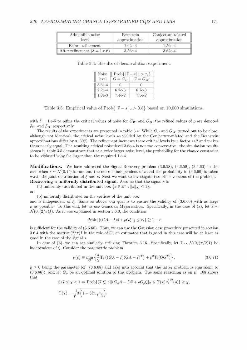
3.6. APPROXIMATING CHANCE CONSTRAINED CQIS AND LMIS 171
Admissible noiselevel
Bernsteinapproximation
Conjecture-relatedapproximation
Before refinement 1.92e-4 1.50e-4After refinement (δ = 1.e-6) 3.56e-4 3.62e-4
Table 3.4: Results of deconvolution experiment.
Noise Prob‖s− s‖2 > τ∗level G = GB G = GW
3.6e-4 0 07.2e-4 6.7e-3 6.7e-31.0e-3 7.4e-2 7.5e-2
Table 3.5: Empirical value of Prob‖s− s‖2 > 0.8 based on 10,000 simulations.
with δ = 1.e-6 to refine the critical values of noise for GW and GB ; the refined values of ρ are denotedρW and ρB , respectively.
The results of the experiments are presented in table 3.4. While GB and GW turned out to be close,although not identical, the critical noise levels as yielded by the Conjecture-related and the Bernsteinapproximations differ by ≈ 30%. The refinement increases these critical levels by a factor ≈ 2 and makesthem nearly equal. The resulting critical noise level 3.6e-4 is not too conservative: the simulation resultsshown in table 3.5 demonstrate that at a twice larger noise level, the probability for the chance constraintto be violated is by far larger than the required 1.e-4.
Modifications. We have addressed the Signal Recovery problem (3.6.58), (3.6.59), (3.6.60) in thecase when s ∼ N (0, C) is random, the noise is independent of s and the probability in (3.6.60) is takenw.r.t. the joint distribution of ξ and s. Next we want to investigate two other versions of the problem.Recovering a uniformly distributed signal. Assume that the signal s is
(a) uniformly distributed in the unit box s ∈ Rn : ‖s‖∞ ≤ 1,or
(b) uniformly distributed on the vertices of the unit boxand is independent of ξ. Same as above, our goal is to ensure the validity of (3.6.60) with as largeρ as possible. To this end, let us use Gaussian Majorization. Specifically, in the case of (a), let s ∼N (0, (2/π)I). As it was explained in section 3.6.3, the condition
Prob‖(GA− I)s + ρGξ‖2 ≤ τ∗ ≥ 1− ε
is sufficient for the validity of (3.6.60). Thus, we can use the Gaussian case procedure presented in section3.6.4 with the matrix (2/π)I in the role of C; an estimator that is good in this case will be at least asgood in the case of the signal s.
In case of (b), we can act similarly, utilizing Theorem 3.16. Specifically, let s ∼ N (0, (π/2)I) beindependent of ξ. Consider the parametric problem
ν(ρ) ≡ minG
π
2Tr
((GA− I)(GA− I)T
)+ ρ2Tr(GGT )
, (3.6.71)
ρ ≥ 0 being the parameter (cf. (3.6.68) and take into account that the latter problem is equivalent to(3.6.66)), and let Gρ be an optimal solution to this problem. The same reasoning as on p. 168 showsthat
6/7 ≤ χ < 1 ⇒ Prob(s, ξ) : ‖(GρA− I)s + ρGρξ‖2 ≤ Υ(χ)ν1/2∗ (ρ) ≥ χ,
Υ(χ) =√
3(1 + 3 ln 1
1−χ
).

172 LECTURE 3: ROBUST CONIC OPTIMIZATION
Applying Theorem 3.16 to the convex set Q = (z, x) : ‖(GρA − I)z + ρGρx‖2 ≤ Υ(χ)ν1/2∗ (ρ) and the
random vectors [s; ξ], [s; ξ], we conclude that
∀(
χ∈[6/7,1)γ>1
): Prob(s, ξ) : ‖(GρA− I)s + ρGρξ‖2 > γΥ(χ)ν1/2
∗ (ρ)
≤ minβ∈[1,γ)
1γ−β
∞∫β
Erf(rErfInv(1− χ))dr.
We conclude that setting
Γ(ρ) = infχ,γ,β
1γ−β
∞∫β
Erf(rErfInv(1− χ))dr :
6/7 ≤ χ < 1, γ > 1
1 ≤ β < γ
γΥ(χ)ν1/2∗ (ρ) ≤ τ∗
[Υ(χ) =
√3
(1 + 3 ln 1
1−χ
)]
(Γ(ρ) = 1 when the right hand side problem is infeasible), one has
Prob(s, ξ) : ‖(GρA− I)s + ρGρξ‖2 > τ∗ ≤ Γ(ρ)
(cf. p. 168). It is easily seen that Γ(·) is a continuous nondecreasing function of ρ > 0 such that Γ(ρ) → 0as ρ → +0, and we end up with the following safe approximation of the Signal Recovery problem:
maxρ
ρ : Γ(ρ) ≤ ε
(cf. (3.6.65)).Note that in the above “Gaussian majorization” scheme we could use the Bernstein approximation,
based on Corollary 2.1, of the chance constraint Prob‖(GA− I)s + ρGξ‖2 ≤ τ∗ ≥ 1− ε instead of theConjecture-related approximation.The case of deterministic uncertain signal. Up to now, signal s was considered as random andindependent of ξ, and the probability in (3.6.60) was taken w.r.t. the joint distribution of s and ξ; asa result, certain “rare” realizations of the signal can be recovered very poorly. Our current goal is tounderstand what happens when we replace the specification (3.6.60) with
∀(s ∈ S) :Probξ : ‖Gu− s‖2 ≤ τ∗ ≡ Probξ : ‖(GA− I)s + ρGξ‖2 ≤ τ∗ ≥ 1− ε,
(3.6.72)
where S ⊂ Rn is a given compact set.Our starting point is the following observation:
Lemma 3.7 Let G, ρ ≥ 0 be such that
Θ ≡ τ2∗
maxs∈S
sT (GA− I)T (GA− I)s + ρ2Tr(GT G)≥ 1. (3.6.73)
Then for every s ∈ S one has
Probζ∼N (0,I) ‖(GA− I)s + ρGζ‖2 > τ∗ ≤ exp− (Θ−1)2
4(Θ+1)
. (3.6.74)
Proof. There is nothing to prove when Θ = 1, so that let Θ > 1. Let us fix s ∈ S and let g = (GA− I)s,W = ρ2GT G, w = ρGT g. We have
Prob‖(GA− I)s + ρGζ‖2 > τ∗ = Prob‖g + ρGζ‖22 > τ2
∗
= ProbζT [ρ2GT G]ζ + 2ζT ρGT g > τ2
∗ − gT g
= ProbζT Wζ + 2ζT w > τ2
∗ − gT g
.
(3.6.75)

3.6. APPROXIMATING CHANCE CONSTRAINED CQIS AND LMIS 173
Denoting by λ the vector of eigenvalues of W , we can assume w.l.o.g. that λ 6= 0, since otherwise W = 0,w = 0 and thus the left hand side in (3.6.75) is 0 (note that τ2
∗ −gT g > 0 due to (3.6.73) and since s ∈ S),and thus (3.6.74) is trivially true. Setting
Ω =τ2∗ − gT g√
λT λ + wT w
and invoking Proposition 2.3, we arrive at
Prob‖(GA− I)s + ρGζ‖2 > τ∗ ≤ exp− Ω2
√λT λ+wT w
4[2√
λT λ+wT w+‖λ‖∞Ω]
= exp− [τ2
∗−gT g]2
4[2[λT λ+wT w]+‖λ‖∞[τ2∗−gT g]]
= exp− [τ2
∗−gT g]2
4[2[λT λ+gT [ρ2GGT ]g]+‖λ‖∞[τ2∗−gT g]]
≤ exp− [τ2
∗−gT g]2
4‖λ‖∞[2[‖λ‖1+gT g]+[τ2∗−gT g]]
,
(3.6.76)
where the concluding inequality is due to ρ2GGT ¹ ‖λ‖∞I and λT λ ≤ ‖λ‖∞‖λ‖1. Further, settingα = gT g, β = Tr(ρ2GT G) and γ = α + β, observe that β = ‖λ‖1 ≥ ‖λ‖∞ and τ2
∗ ≥ Θγ ≥ γ by (3.6.73).It follows that
[τ2∗ − gT g]2
4‖λ‖∞ [2[‖λ‖1 + gT g] + [τ2∗ − gT g]]≥ (τ2
∗ − γ + β)2
4β(τ2∗ + γ + β)≥ (τ2
∗ − γ)2
4γ(τ2∗ + γ),
where the concluding inequality is readily given by the relations τ2∗ ≥ γ ≥ β > 0. Thus, (3.6.76) implies
that
Prob‖(GA− I)s + ρGζ‖2 > τ∗ ≤ exp− (τ2
∗ − γ)2
4γ(τ2∗ + γ)
≤ exp
− (Θ− 1)2
4(Θ + 1)
. ¤
Lemma 3.7 suggests a safe approximation of the problem of interest as follows. Let Θ(ε) > 1 be givenby
exp− (Θ− 1)2
4(Θ + 1) = ε [⇒ Θ(ε) = (4 + o(1)) ln(1/ε) as ε → +0]
and letφ(G) = max
s∈SsT (GA− I)T (GA− I)s, (3.6.77)
(this function clearly is convex). By Lemma 3.7, the optimization problem
maxρ,G
ρ : φ(G) + ρ2Tr(GT G) ≤ γ∗ ≡ Θ−1(ε)τ2
∗
(3.6.78)
is a safe approximation of the problem of interest. Applying bisection in ρ, we can reduce this problemto a “short series” of convex feasibility problems of the form
find G: φ(G) + ρ2Tr(GT G) ≤ γ∗. (3.6.79)
Whether the latter problems are or are not computationally tractable depends on whether the functionφ(G) is so, which happens if and only if we can efficiently optimize positive semidefinite quadratic formssT Qs over S.
Example 3.8 Let S be an ellipsoid centered at the origin:
S = s = Hv : vT v ≤ 1

174 LECTURE 3: ROBUST CONIC OPTIMIZATION
In this case, it is easy to compute φ(G) — this function is semidefinite representable:
φ(G) ≤ t ⇔ maxs∈S
sT (GA− I)T (GA− I)s ≤ t
⇔ maxv:‖v‖2≤1
vT (HT (GA− I)T (GA− I)Hv ≤ t
⇔ λmax(HT (GA− I)T (GA− I)H) ≤ t
⇔ tI −HT (GA− I)T (GA− I)H º 0 ⇔[
tI HT (GA− I)T
(GA− I)H I
]º 0,
where the concluding ⇔ is given by the Schur Complement Lemma. Consequently, (3.6.79) is the effi-ciently solvable convex feasibility problem
Find G, t: t + ρ2Tr(GT G) ≤ γ∗,[
tI HT (GA− I)T
(GA− I)H I
]º 0.
Example 3.8 allows us to see the dramatic difference between the case where we are interested in “highlyreliable with high probability” recovery of a random signal and “highly reliable” recovery of everyrealization of uncertain signal. Specifically, assume that G, ρ are such that (3.6.60) is satisfied withs ∼ N (0, In). Note that when n is large, s is nearly uniformly distributed over the sphere S of radius√
n (indeed, sT s =∑i
s2i , and by the Law of Large Numbers, for δ > 0 the probability of the event
‖s‖2 6∈ [(1−δ)√
n, (1+δ)√
n] goes to 0 as n →∞, in fact exponentially fast. Also, the direction s/‖s‖2of s is uniformly distributed on the unit sphere). Thus, the recovery in question is, essentially, a highlyreliable recovery of random signal uniformly distributed over the above sphere S. Could we expect therecovery to “nearly satisfy” (3.6.72), that is, to be reasonably good in the worst case over the signalsfrom S? The answer is negative when n is large. Indeed, a sufficient condition for (3.6.60) to be satisfiedis
Tr((GA− I)T (GA− I)) + ρ2Tr(GT G) ≤ τ2∗
O(1) ln(1/ε)(∗)
with appropriately chosen absolute constant O(1). A necessary condition for (3.6.72) to be satisfied is
nλmax((GA− I)T (GA− I)) + ρ2Tr(GT G) ≤ O(1)τ2∗ . (∗∗)
Since the trace of the n× n matrix Q = (GA− I)T (GA− I) can be nearly n times less than nλmax(Q),the validity of (∗) by far does not imply the validity of (∗∗). To be more rigorous, consider the case whenρ = 0 and GA− I = Diag1, 0, ..., 0. In this case, the ‖ · ‖2-norm of the recovering error, in the case ofs ∼ N (0, In), is just |s1|, and Prob|s1| > τ∗ ≤ ε provided that τ∗ ≥
√2 ln(2/ε), in particular, when
τ∗ =√
2 ln(2/ε). At the same time, when s =√
n[1; 0; ...; 0] ∈ S, the norm of the recovering error is√
n,which, for large n, is incomparably larger than the above τ∗.
Example 3.9 Here we consider the case where φ(G) cannot be computed efficiently, specifically, the casewhere S is the unit box Bn = s ∈ Rn : ‖s‖∞ ≤ 1 (or the set Vn of vertices of this box). Indeed, it isknown that for a general-type positive definite quadratic form sT Qs, computing its maximum over the unitbox is NP-hard, even when instead of the precise value of the maximum its 4%-accurate approximationis sought. In situations like this we could replace φ(G) in the above scheme by its efficiently computableupper bound φ(G). To get such a bound in the case when S is the unit box, we can use the followingwonderful result:
Nesterov’s π2 Theorem [76] Let A ∈ Sn
+. Then the efficiently computable quantity
SDP(A) = minλ∈Rn
∑
i
λi : Diagλ º A
is an upper bound, tight within the factor π2 , on the quantity
Opt(A) = maxs∈Bn
sT As.

3.7. EXERCISES 175
Assuming that S is Bn (or Vn), Nesterov’s π2 Theorem provides us with an efficiently computable and
tight, within the factor π2 , upper bound
φ(G) = minλ
∑
i
λi :[
Diag(λ) (GA− I)T
GA− I I
]º 0
on φ(G). Replacing φ(·) by its upper bound, we pass from the intractable problems (3.6.79) to theirtractable approximations
find G,λ:∑
i
λi + ρ2Tr(GT G) ≤ γ∗,[
Diag(λ) (GA− I)T
GA− I I
]º 0; (3.6.80)
we then apply bisection in ρ to rapidly approximate the largest ρ = ρ∗, along with the associated G = G∗,for which problems (3.6.80) are solvable, thus getting a feasible solution to the problem of interest.
3.7 Exercises
Exercise 3.1 Consider a semi-infinite conic constraint
∀(ζ ∈ ρZ) : a0[x] +L∑
`=1
ζia`[x] ∈ Q (CZ [ρ])
Assume that for certain ϑ and some closed convex set Z∗, 0 ∈ Z∗, the constraint (CZ∗ [·]) admitsa safe tractable approximation tight within the factor ϑ. Now let Z be a closed convex set thatcan be approximated, up to a factor λ, by Z∗, meaning that for certain γ > 0 we have
γZ∗ ⊂ Z ⊂ (λγ)Z∗.
Prove that (CZ [·]) admits a safe tractable approximation, tight within the factor λϑ.
Exercise 3.2 Let ϑ ≥ 1 be given, and consider the semi-infinite conic constraint (CZ [·]) “asa function of Z,” meaning that a`[·], 0 ≤ ` ≤ L, and Q are once and forever fixed. In whatfollows, Z always is a solid (convex compact set with a nonempty interior) symmetric w.r.t. 0.
Assume that whenever Z is an ellipsoid centered at the origin, (CZ [·]) admits a safe tractableapproximation tight within factor ϑ (as it is the case for ϑ = 1 when Q is the Lorentz cone, seesection 3.2.5).
1. Prove that when Z is the intersection of M centered at the origin ellipsoids:
Z = ζ : ζT Qiζ ≤ 1, i = 1, ..., M [Qi º 0,∑
i Qi  0]
(CZ [·]) admits a safe tractable approximation tight within the factor√
Mϑ.
2. Prove that if Z = ζ : ‖ζ‖∞ ≤ 1, then (CZ [·]) admits a safe tractable approximationtight within the factor ϑ
√dim ζ.
3. Assume that Z is the intersection of M ellipsoids not necessarily centered at the origin.Prove that then (CZ [·]) admits a safe tractable approximation tight within a factor
√2Mϑ.

176 LECTURE 3: ROBUST CONIC OPTIMIZATION
Exercise 3.3 Consider the situation as follows (cf. section 3.2.6). We are given an observation
y = Ax + b ∈ Rm
of unknown signal x ∈ Rn. The matrix B ≡ [A; b] is not known exactly; all we know is thatB ∈ B = B = Bn + LT ∆R : ∆ ∈ Rp×q, ‖∆‖2,2 ≤ ρ. Build an estimate v of the vector Qx,where Q is a given k × n matrix, that minimizes the worst-case, over all possible true values ofx, ‖ · ‖2 estimation error.
Exercise 3.4 Consider an uncertain Least Squares inequality
‖A(η)x + b(η)‖2 ≤ τ, η ∈ ρZwhere Z, 0 ∈ intZ, is a symmetric w.r.t. the origin convex compact set that is the intersectionof J > 1 ellipsoids not necessarily centered at the origin:
Z = η : (η − aj)T Qj(η − aj) ≤ 1, 1 ≤ j ≤ J [Qj º 0,∑
j Qj  0]
Prove that the RC of the uncertain inequality in question admits a safe tractable approximationtight within the factor O(1)
√lnJ (cf. Theorem 3.9).
Exercise 3.5 [Robust Linear Estimation, see [44]] Let a signal v ∈ Rn be observed accordingto
y = Av + ξ,
where A is an m× n matrix, known up to “unstructured norm-bounded perturbation”:
A ∈ A = A = An + LT ∆R : ∆ ∈ Rp×q, ‖∆‖2,2 ≤ ρ,and ξ is a zero mean random noise with a known covariance matrix Σ. Our a priori informationon v is that
v ∈ V = v : vT Qv ≤ 1,where Q Â 0. We are looking for a linear estimate
v = Gy
with the smallest possible worst-case mean squared error
EstErr = supv∈V,A∈A
(E
‖G[Av + ξ]− v‖22
)1/2
(cf. section 3.2.6).1) Reformulate the problem of building the optimal estimate equivalently as the RC of
uncertain semidefinite program with unstructured norm-bounded uncertainty and reduce thisRC to an explicit semidefinite program.
2) Assume that m = n, Σ = σ2In, and the matrices ATn An and Q commute, so that An =
V DiagaUT and Q = UDiagqUT for certain orthogonal matrices U, V and certain vectorsa ≥ 0, q > 0. Let, further, A = An + ∆ : ‖∆‖2,2 ≤ ρ. Prove that in the situation in questionwe lose nothing when looking for G in the form of
G = UDiaggV T ,
and build an explicit convex optimization program with just two variables specifying the optimalchoice of G.
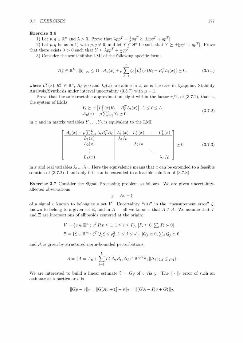
3.7. EXERCISES 177
Exercise 3.61) Let p, q ∈ Rn and λ > 0. Prove that λppT + 1
λqqT º ±[pqT + qpT ].2) Let p, q be as in 1) with p, q 6= 0, and let Y ∈ Sn be such that Y º ±[pqT + qpT ]. Prove
that there exists λ > 0 such that Y º λppT + 1λqqT .
3) Consider the semi-infinite LMI of the following specific form:
∀(ζ ∈ RL : ‖ζ‖∞ ≤ 1) : An(x) + ρL∑
`=1
ζ`
[LT
` (x)R` + RT` L`(x)
] º 0, (3.7.1)
where LT` (x), RT
` ∈ Rn, R` 6= 0 and L`(x) are affine in x, as is the case in Lyapunov StabilityAnalysis/Synthesis under interval uncertainty (3.5.7) with µ = 1.
Prove that the safe tractable approximation, tight within the factor π/2, of (3.7.1), that is,the system of LMIs
Y` º ± [LT
` (x)R` + RT` L`(x)
], 1 ≤ ` ≤ L
An(x)− ρ∑L
`=1 Y` º 0(3.7.2)
in x and in matrix variables Y1, ..., YL is equivalent to the LMI
An(x)− ρ∑L
`=1 λ`RT` R` LT
1 (x) LT2 (x) · · · LT
L(x)L1(x) λ1/ρL2(x) λ2/ρ
.... . .
LL(x) λL/ρ
º 0 (3.7.3)
in x and real variables λ1..., λL. Here the equivalence means that x can be extended to a feasiblesolution of (3.7.2) if and only if it can be extended to a feasible solution of (3.7.3).
Exercise 3.7 Consider the Signal Processing problem as follows. We are given uncertainty-affected observations
y = Av + ξ
of a signal v known to belong to a set V . Uncertainty “sits” in the “measurement error” ξ,known to belong to a given set Ξ, and in A — all we know is that A ∈ A. We assume that Vand Ξ are intersections of ellipsoids centered at the origin:
V = v ∈ Rn : vT Piv ≤ 1, 1 ≤ i ≤ I, [Pi º 0,∑
i Pi  0]
Ξ = ξ ∈ Rm : ξT Qjξ ≤ ρ2ξ , 1 ≤ j ≤ J, [Qj º 0,
∑j Qj º 0]
and A is given by structured norm-bounded perturbations:
A = A = An +L∑
`=1
LT` ∆`R`, ∆` ∈ Rp`×q` , ‖∆`‖2,2 ≤ ρA.
We are interested to build a linear estimate v = Gy of v via y. The ‖ · ‖2 error of such anestimate at a particular v is
‖Gy − v‖2 = ‖G[Av + ξ]− v‖2 = ‖(GA− I)v + Gξ‖2,

178 LECTURE 3: ROBUST CONIC OPTIMIZATION
and we want to build G that minimizes the worst, over all v,A, ξ compatible with our a prioriinformation, estimation error
maxξ∈Ξ,v∈V,A∈A
‖(GA− I)v + Gξ‖2.
Build a safe tractable approximation of this problem that seems reasonably tight when ρξ andρA are small.