Embed Size (px)
Citation preview
ROBUST BIRD-STRIKE MODELING USING LS-DYNA
by
Carlos Alberto Huertas-Ortecho
A thesis submitted in partial fulfillment of the requirements for the degree of
MASTER OF SCIENCE in
MECHANICHAL ENGINEERING
UNIVERSITY OF PUERTO RICO MAYAGÜEZ CAMPUS
2006 Approved by: ________________________________ Gustavo Gutierrez, Ph.D. Member, Graduate Committee
__________________
Date
________________________________ Frederick Just, Ph.D. Member, Graduate Committee
__________________ Date
________________________________ Vijay K. Goyal, Ph.D. Chair, Graduate Committee
__________________ Date
________________________________ Damaris Santana Morant, Ph.D. Representative of Graduate Studies
__________________ Date
________________________________ Paul Sundaram, Ph.D. Chairperson of the Department
__________________ Date

UMI Number: 1435268
14352682006
UMI MicroformCopyright
All rights reserved. This microform edition is protected against unauthorized copying under Title 17, United States Code.
ProQuest Information and Learning Company 300 North Zeeb Road
P.O. Box 1346 Ann Arbor, MI 48106-1346
by ProQuest Information and Learning Company.

Abstract
Throughout this work, bird-strike events are studied using three approaches in LS-
DYNA: Lagrangian, Arbitrary Lagrange Eulerian (ALE), and Smooth Particle
Hydrodynamics (SPH). A simple one-dimensional beam centered impact problem was solved
analytically to validate the results produced by LS-DYNA using the three mentioned
methods. All three approaches in LS-DYNA produced results within 7% error when
compared with the analytical solution. Bird-strike events, soft-body impact problems, are
divided into three separate problems: frontal impact on rigid flat plate, 0 degree impact on
deformable tapered plate, and 30 degree impact on deformable tapered plate. The bird model
is modeled as a cylinder. Throughout the study, the most influencing parameters have been
identified and peak pressures and forces are compared to those results available in the
literature. The case for 0 degrees tapered plate impact shows little bird-plate interaction
because the bird is sliced in two parts and the results from all three methods employed are
within 10% difference from the test data available in the literature. For the frontal impact on
rigid plate, all three methods are validated with the test data within 10% error. Overall,
Lagrangia, ALE and SPH methods can be used for the analysis of bird-strike events.

Resumen
A través de este trabajo, el impacto de aves es estudiado utilizando tres formulaciones en LS-
DYNA: Lagrangiano, Lagrange-Euler Arbitrario (ALE), e Hidrodinámica de Partículas
Suavizadas (SPH) por sus siglas en inglés. Un problema simple uní-dimensional del impacto
central en una viga fue resuelto analíticamente para validar los resultados producidos por LS-
DYNA usando los tres métodos mencionados. Los tres métodos en LS-DYNA dieron
resultados dentro de un margen de error del 7% al compararlo con la solución analítica. Los
impactos de ave, problema de impacto de cuerpos blandos, son divididos en tres problemas
separados: Impacto frontal contra placas planas rígidas, impacto a 0 grados en placas
afiladas deformables e impacto a 30 grados en placas afiladas deformables. El ave es
modelada como un cilindro. A lo largo del presente estudio, los parámetros con mas
influencia fueron identificados y las presiones y fuerzas picos fueron comparados con las
disponibles en la literatura. En el caso de impacto a 0 grados en una placa afilada la placa
presenta muy poca interacción con el ave debido a que el ave es dividida en dos partes y los
resultados de los tres métodos utilizados están dentro del 10% de diferencia comparada con
los datos experimentales disponibles en la literatura. Para el impacto frontal contra placas
rígidas, los tres métodos fueron validados con los resultados experimentales dentro de un
margen de error del 10%. En general, los métodos de Lagrange, ALE y SPH pueden ser
utilizados en el análisis de impacto de aves.

Dedication
To my Lord Jesus, my family and close friends.

v
Acknowledgements
During my graduate studies at the University of Puerto Rico at Mayagüez, several persons
have collaborated direct and indirectly with my thesis. Without their help it would have been
impossible to complete this work. First and foremost, I would like to begin by expressing my
sincere gratitude to my advisor, Dr. Vijay K. Goyal, for giving me the opportunity to conduct
my master’s degree under his guidance and supervision. Dr. Goyal has provided motivation,
encouragement, and support throughout my studies.
Next, I am most thankful to United Technologies Co. for funding this research and providing
the necessary resources. I gratefully acknowledge the technical discussions with Dr. Thomas
J. Vasko and the grant monitors for providing the necessary computational resources.
Special thanks to Dr. Mhamed Souli, Professor University d’Artois in France, for the
technical discussions regarding the ALE models in LS-DYNA and to Dr. Luis Suarez,
Professor of UPRM, for verifying the analytical solution to the beam centered problem. Also,
I am thankful to all the undergraduate students who participated in this research: José
Borrero, Tomás Leutwiler and José Irizarry. Without them this work would have fell short.
At last, and the most important acknowledgement goes to God, to my family and to my close
friends, for their unconditional support, inspiration and love throughout the distance.
vi
Table of Contents Table of Contents..................................................................................................................... vi
List of Tables ......................................................................................................................... viii
Figure List................................................................................................................................ ix
Figure List................................................................................................................................ ix
Chapter 1. Preliminary Remarks................................................................................................1 1.1 Literature Review.......................................................................................................................... 2 1.2 Objectives of the present work...................................................................................................... 9 1.3 Outline of the Thesis ................................................................................................................... 10
Chapter 2. Impact Analysis......................................................................................................12 2.1 A Continuum Approach .............................................................................................................. 12
2.1.1 Governing Equations..........................................................................................................................13 2.1.2 Lagrangian Approach.........................................................................................................................20 2.1.3 ALE Approach ...................................................................................................................................26 2.1.4 SPH Formulation ...............................................................................................................................30
2.2 Beam Centered Impact Problem ................................................................................................. 38 2.2.1 Analytical solution .............................................................................................................................39 2.2.2 Lagrange simulation...........................................................................................................................46 2.2.3 ALE simulation of the beam centered impact ....................................................................................49 2.2.4 SPH simulation of the beam centered impact ....................................................................................51
2.3 Bird-Strike Impact Problem ........................................................................................................ 53 2.3.1 LS-DYNA for Bird-Strike Events......................................................................................................54 2.3.2 General Bird and Target Model Properties ........................................................................................56 2.3.3 Test Data for Bird-Strike Event .........................................................................................................59
Chapter 3. Bird-Strike Modeling Based on Lagrangian Formulation......................................68 3.1 Current Lagrangian Bird Model.................................................................................................. 68
3.1.1 Pre-processing variables for the Lagrangian model ...........................................................................68 3.2 Bird Impact against a Flat Rigid Plate ........................................................................................ 71
3.2.1 Using *MAT_ELASTIC_FLUID ......................................................................................................71 3.2.2 Using *MAT_ELASTIC_FLUID ......................................................................................................78 3.2.3 Comparison of the Lagrangian Simulations.......................................................................................81 3.2.4 Impact for a Tapered Plate (Impact at 30º) ........................................................................................84 3.2.5 Impact Simulation for a Tapered Plate (at 0º) ....................................................................................90
Chapter 4. Bird-Strike Modeling Based on SPH Formulation ................................................95 4.1 SPH Model for the Bird-Strike Event ......................................................................................... 96
4.1.1 Pre-processing variables for the SPH model......................................................................................96 4.2 Bird-Strike Simulation ................................................................................................................ 98
4.2.1 SPH element generation.....................................................................................................................98 4.3 Bird-Strike Against Rigid Flat Plate ......................................................................................... 100
4.3.1 Parameter Variation for SPH Modeling ...........................................................................................100 4.3.2 Contact Variation for 8700 SPH particles........................................................................................106 4.3.3 Changing the number of SPH particles ............................................................................................123

vii
4.4 Impact for a Tapered Plate Impact at 0º .................................................................................... 130 4.5 Impact for a Tapered Plate at 30º .............................................................................................. 137 4.6 Computational Time Employed ................................................................................................ 144 4.7 Comparison of the Total Energy .............................................................................................. 145 4.8 Advantages and Disadvantages................................................................................................. 146 4.9 Best Approach for Bird-Strike Event Modeling........................................................................ 149
Chapter 5. Bird-Strike Modeling Based on ALE Formulation ..............................................151 5.1 ALE Model for the Bird-Strike Event....................................................................................... 151
5.1.1 Pre-Processing in the ALE Formulation ..........................................................................................153 5.2 Bird Impact Against a Flat Plate ............................................................................................... 153
5.2.1 Bird Strike Simulation Using 2D ALE.............................................................................................154 5.2.2 2D ALE Simulation of Shot 5126A.................................................................................................156 5.2.3 Bird Strike Simulation Using ALE in 3D ........................................................................................160 5.2.4 Variation of the Time Step Scale Factor ..........................................................................................166
5.3 Bird-strike simulation in tapered plate ...................................................................................... 171 5.3.1 Simulation for Tapered Plate Impact at 0° .......................................................................................171 5.3.2 ALE Simulation for Tapered Plate Impact at 30° ............................................................................175
Chapter 6. Concluding Remarks ............................................................................................181 6.1 Conclusions ............................................................................................................................... 181 6.2 Recommendations for Future work........................................................................................... 183
References..............................................................................................................................184
Appendix A. LS-DYNA Overview.......................................................................................189 A.1 Features .................................................................................................................................... 189 A.2 Lagrangian Approach in LS-DYNA ........................................................................................ 192 A.3 ALE Approach in LS-DYNA................................................................................................... 199
A.3.2 Code explanation.............................................................................................................................201 A.4 SPH Approach in LS-DYNA ................................................................................................... 208
A.4.1 SPH code explanation .....................................................................................................................210 Appendix B. Keyword for the 3D Lagrangian Simulation ....................................................214
Appendix C. Keyword for the 2D ALE Simulation ..............................................................219

viii
List of Tables Table 2.1: Comparison of the impulsive pressure for Lagrange............................................. 48 Table 2.2: Comparison of the impulsive pressure for ALE.................................................... 50 Table 2.3: Comparison of the impulsive pressure .................................................................. 52 Table 2.4: Properties for the model of bird............................................................................. 56 Table 2.5: Tapered plate properties (fixed at the two shortest sides) ..................................... 58 Table 3.1: Bird model used for the Lagrangian simulations in this project............................ 69 Table 3.2: Constants for the *EOS_TABULATED equation of state. ................................... 70 Table 3.3: Peak impact pressure comparison for Lagrange simulations ................................ 83 Table 3.4: Thickness for each part for the tapered plate......................................................... 85 Table 3.5: Maximum normal deflection comparison.............................................................. 90 Table 3.6: Maximum force comparison for 0 degrees impact using Lagrange. ..................... 94 Table 4.1: SPH bird model...................................................................................................... 97 Table 4.2: Comparison between SPH and Lagrangian simulations using a rigid wall......... 112 Table 4.3: Comparison of results between the SPH simulation with two targets and the
Lagrangian simulation .................................................................................................. 116 Table 4.4: Pressure comparison between SPH and Lagrangian simulations ........................ 122 Table 4.5: Comparison of peak force values for the simulations performed........................ 123 Table 4.6: Pressure comparison for particle variation in the SPH simulations. ................... 125 Table 4.7: Peak force comparison for various SPH tapered plate impact at 0 degrees. ....... 136 Table 4.8: Force and maximum normal deflection comparison for various SPH tapered plate
impact at 30 degrees...................................................................................................... 143 Table 5.1: Bird model used for the ALE simulation............................................................. 152 Table 5.2: Comparison of peak pressure for different Lagrange, SPH and ALE simulations.
....................................................................................................................................... 169 Table 5.3: Comparison of peak forces for different Lagrange, SPH and ALE tapered plate
impact simulations at 0 degrees. ................................................................................... 179 Table 5.4: Comparison of peak forces for different Lagrange, SPH and ALE tapered plate
impact simulations at 30 degrees. ................................................................................. 180
ix
Figure List
Figure 2.1: Pressure evaluation model.................................................................................... 16 Figure 2.2: Pressure evaluation model.................................................................................... 19 Figure 2.3: Lagrangian mesh. ................................................................................................. 20 Figure 2.4: Example of Lagrangian mesh deformation .......................................................... 21 Figure 2.5: Description of motion for Lagrange formulation ................................................. 21 Figure 2.6: Lagrangian deformation for a soft body impact simulation. ................................ 24 Figure 2.7: Description of motion for Eulerian formulation................................................... 26 Figure 2.8: Mapping between the material and the spatial domain for an Eulerian description.
......................................................................................................................................... 27 Figure 2.9: Description of motion for Arbitrary Lagrange Eulerian formulation................... 28 Figure 2.10: Maps between material, spatial and referential domains. .................................. 29 Figure 2.11: Soft body impact using ALE. ............................................................................. 29 Figure 2.12: Integration cycle in time of the SPH computation process ................................ 34 Figure 2.13: Neighbor search particles inside a 2h radius sphere........................................... 36 Figure 2.14: SPH simulation for a soft body impact. ............................................................. 37 Figure 2.15: Beam impact problem. ....................................................................................... 38 Figure 2.16: Beam impact problem simplification. ................................................................ 39 Figure 2.17: Plastic deformation after collision...................................................................... 40 Figure 2.18: Impulse for a given force time history. .............................................................. 41 Figure 2.19: Average impact force. ........................................................................................ 42 Figure 2.20: Visualization of the theorem of impulse and momentum. ................................. 42 Figure 2.21: One degree of freedom damped vibrating system.............................................. 44 Figure 2. 22: Considering the continuous beam impact problem. .......................................... 45 Figure 2.23: Lagrange simulation of transversal beam impact............................................... 47 Figure 2.24: Impact force for the Lagrangian simulation ....................................................... 47 Figure 2.25: ALE simulation of transversal beam impact ...................................................... 49 Figure 2.26: Force plot for ALE simulation ........................................................................... 50 Figure 2.27: SPH simulation of transversal beam impact....................................................... 51 Figure 2.28: Force plot for SPH simulation............................................................................ 52 Figure 2.29: Force plot for SPH simulation............................................................................ 54 Figure 2.30: Histogram for the bird masses of the Barber et al. (1975) bird impact research.60 Figure 2.31: Histogram for the bird velocities of the Barber et al. (1975) bird impact research.
......................................................................................................................................... 60 Figure 2.32: Histogram for the bird impact peak pressures of the Barber et al. (1975) bird
impact research. .............................................................................................................. 61 Figure 2.33: Pressure – Time oscillograph for shot 4992-B (Barber et al., 1975).................. 62 Figure 2.34: Manipulation of the Pressure- Time oscillograph for shot 4992-B analyzed in
MatLab (Barber et al., 1975)........................................................................................... 63 Figure 2.35: Pressure vs. time distribution for Shot 4992B (Barber et al., 1975) .................. 63 Figure 2.36: Pressure vs. time distribution for Shot 5181C (Barber et al., 1975) .................. 64 Figure 2.37: Pressure vs. time distribution for Shot 5126A (Barber et al., 1975) .................. 64 Figure 2.38: Pressure vs. time distribution for Shot 5172C.................................................... 65

x
Figure 2.39: Pressure vs. time distribution for Shot 5127A ................................................... 65 Figure 2.40: Pressure vs. time distribution for Shot 5113A ................................................... 66 Figure 2.41: Pressure vs. time distribution for Shot 5129A ................................................... 66 Figure 3.1: Geometric model for the Lagrangian bird and target shell. ................................. 71 Figure 3.2: Deformation of the bird model for the Lagrangian simulation using the
ERODING_NODES_TO _SURFACE contact .............................................................. 72 Figure 3.3: Force plot for the Lagrangian simulation using the
ERODING_NODES_TO_SURFACE contact ............................................................... 72 Figure 3.4: Global change in mass for the Lagrangian simulation. ........................................ 73 Figure 3.5: Resultant force in the interface for the Lagrange frontal impact on a rigid flat
plate................................................................................................................................. 74 Figure 3.6: Deformation of the bird model for the Lagrangian simulation using
the FORMING_NODES_TO _SURFACE contact ........................................................ 75 Figure 3.7: Force plot for the Lagrangian simulation using the
FORMING_NODES_TO_SURFACE contact............................................................... 75 Figure 3.8: Deformation of the bird model for the Lagrangian simulation using the
NODES_TO_SURFACE contact ................................................................................... 77 Figure 3.9: Force plot for the Lagrangian simulation using the NODES_TO_SURFACE
contact. ............................................................................................................................ 77 Figure 3.10: Lagrangian bird deformation when using *MAT_ELASTIC_FLUID .............. 78 Figure 3.11: Diameter in the peak force impact time. ............................................................ 79 Figure 3.12: Force plot for the Lagrangian case using elastic fluid material. ........................ 79 Figure 3.13: Force plot for the Lagrangian case using elastic fluid material. ........................ 80 Figure 3.14: Force plot for the Lagrangian case using elastic fluid material. ........................ 81 Figure 3.15: Comparison of the Lagrangian simulations using *MAT_NULL ................... 82 Figure 3.16: Comparison of the Lagrangian simulations for *MAT_ELASTIC_FLUID.... 84 Figure 3.17: Lagrangian bird model impacting the tapered plate at 30º................................. 86 Figure 3.18: Bird impacting a tapered plate at 30º and at different time intervals. ................ 86 Figure 3.19: Top view of the deformed tapered plate leading edge after the impact of the
Lagrangian bird at 30º..................................................................................................... 87 Figure 3.20: Resultant force for the Lagrange simulation of the impact of a bird against a
tapered plate with an angle of 30 degrees....................................................................... 87 Figure 3.21: Bird impacting a tapered plate at 30º and at different time intervals. ................ 88 Figure 3.22: Top view of the deformed tapered plate leading edge after the impact of the
Lagrangian bird at 30º..................................................................................................... 89 Figure 3.23: Resultant force for the Lagrange simulation of the impact of a bird against a
tapered plate with an angle of 30 degrees....................................................................... 89 Figure 3.24: Model of the tapered plate for the Lagrangian impact simulation. .................... 91 Figure 3.25: Deformation of the tapered plate at different time intervals for the Lagrange
description....................................................................................................................... 91 Figure 3.26: Top view of the tapered plate deflection at the leading edge for the Lagrange
simulation at 0º. .............................................................................................................. 92 Figure 3.27: Plot of the resultant force for the Lagrange simulation of the impact of a bird at
0 degrees against a tapered plate..................................................................................... 92
xi
Figure 3.28: Interaction of the bird and the tapered plate for 0 degrees................................. 93 Figure 3.29: Force plot for the Lagrange tapered plate impact at 0 using
*MAT_ELASTIC_FLUID ............................................................................................. 93 Figure 4.1: SPH element generation for the bird model ......................................................... 99 Figure 4.2: Side view of the simulation for
*CONTACT_AUTOMATIC_NODE_TO_SURFACE and FORM=0........................ 102 Figure 4.3: Simulation results for the SPH with FORM=0 and
*CONTACT_AUTOMATIC_NODE_TO_SURFACE. .............................................. 102 Figure 4.4: Sequence at different time intervals of deformation of the SPH bird (FORM=1
and *CONTACT_AUTOMATIC_NODE_TO_SURFACE). ...................................... 103 Figure 4.5: Resultant force for SPH simulation with FORM=1 and
*CONTACT_AUTOMATIC_NODE_TO_SURFACE. .............................................. 104 Figure 4.6: Deformation of the SPH bird for different time intervals (NCBS= 2)............... 104 Figure 4.7: Resultant force in the interface for the SPH simulation of the bird-strike
(NCBS=2) and Constraint contact type. ....................................................................... 105 Figure 4.8: Deformation of the SPH bird for different time intervals (NCBS= 5)............... 105 Figure 4.9: Resultant force in the interface for the SPH simulation of the bird-strike
(NCBS=5) ..................................................................................................................... 106 Figure 4.10: Top view of the created SPH particles and the original solid mesh................. 107 Figure 4.11: Side view of the cylinder impacting the plate at different time intervals
(*CONCTACT_ERODING_NODE_TO_SURFACE)................................................ 107 Figure 4.12: Resultant force for SPH simulation with
*CONCTACT_ERODING_NODE_TO_SURFACE and FORM=1. .......................... 108 Figure 4.13: Mass plot during the impact event with FORM=1 and
*CONTACT_ERODING_NODE_TO_SURFACE ..................................................... 109 Figure 4.14: Side view of the cylinder impacting the plate at different time intervals
(*CONCTACT_FORMING_NODE_TO_SURFACE and FORM=1) ........................ 110 Figure 4.15: Force for SPH simulation using forming contact type. .................................... 110 Figure 4.16: SPH progression of the bird deformation for a rigid wall contact. .................. 111 Figure 4.17: Resultant normal force using the rigid wall contact......................................... 112 Figure 4.18: Deformation of the SPH Bird and the plates.................................................... 114 Figure 4.19: Resultant force in the interface of the bird and the targets. a) Bottom plate, b)
Top plate ....................................................................................................................... 114 Figure 4.20: Deformation of the SPH bird for *MAT_RIGID............................................. 117 Figure 4.21: Resultant force in the interface of the bird and the target for *MAT_RIGID.. 117 Figure 4.22: Deformation of the SPH bird at different time intervals. ................................. 118 Figure 4.23: Top view of the impact of the SPH particles against the transducer................ 119 Figure 4.24: Resultant force in the interface for the SPH simulation................................... 119 Figure 4.25: Pressure in the interface for the SPH simulation.............................................. 120 Figure 4.26: Mass variation plot during the impact event with FORM=1 and
*CONCTACT_CONSTRAINT_NODE_TO_SURFACE ........................................... 121 Figure 4.27: Comparison of pressure plots for Lagrangian and SPH simulation using
constraint contact type for 8700 particles. .................................................................... 122 Figure 4.28: SPH simulations of shot 5126 A for different number of particles.................. 126

xii
Figure 4.29: SPH simulations of shot 5126 A for different number of particles.................. 128 Figure 4.30: Force plot comparison of different SPH simulations using a rigid wall contact
type................................................................................................................................ 128 Figure 4.31: Comparison of peak pressure obtained in Lagrangian and SPH simulation using
the nodes to surface contact TEROD=1.1 .................................................................... 129 Figure 4.32: Cross section of the model for tapered plate impact using a higher density of
SPH particles................................................................................................................. 131 Figure 4.33: Resultant force for the SPH simulation at 0 degrees using material null......... 132 Figure 4.34: Result of the interaction for the SPH simulation of the tapered plate impact
using material null......................................................................................................... 132 Figure 4.35: Deformed plate after the 0 degrees impact of the SPH bird............................. 133 Figure 4.36: Front view of the deformed plate after the 0 degrees impact of the SPH bird
using material null......................................................................................................... 133 Figure 4.37: Result of the interaction for the SPH simulation of the tapered plate.............. 134 Figure 4.38: Front view of the deformed plate after the 0 degrees impact of the SPH bird
using material elastic fluid. ........................................................................................... 135 Figure 4.39: Resultant force for the SPH simulation at 0 degrees using material elastic fluid.
....................................................................................................................................... 135 Figure 4.40: Side view of the SPH simulation for the bird impacting a plate at 30º. ........... 137 Figure 4.41: Deformation of the tapered plate using material null and 26195 SPH particles.
....................................................................................................................................... 138 Figure 4.42: Top view of the deformed plate after the impact of the bird with an angle of 30
degrees. ......................................................................................................................... 138 Figure 4.43: Side view of the tapered plate leading edge. .................................................... 139 Figure 4.44: Resultant force in the interface for the impact of the bird on a tapered plate with
an angle of 30 degrees (SPH simulation)...................................................................... 139 Figure 4.45: Deformation of the tapered plate at different times of the simulation (30 degrees
and 8700 SPH particles)................................................................................................ 140 Figure 4.46: Top view of the deformed plate after the impact of the bird with an angle of 30
degrees and 8700 particles. ........................................................................................... 141 Figure 4.47: Deformation of the tapered plate at different times of the simulation (30 degrees
and 8700 SPH particles)................................................................................................ 142 Figure 4.48: Top view of the deformed plate after the impact of the bird using mat null.... 142 Figure 4.49: Resultant force in the interface for the impact of the bird on a tapered plate with
an angle of 30 degrees (SPH simulation)...................................................................... 143 Figure 4.50: Elapsed simulation time for Lagrange and SPH methods and impact types.... 144 Figure 4.51: Plot of the total, internal, and kinetic energy for the SPH and Lagrangian
simulations .................................................................................................................... 145 Figure 5.1: Deformation of the shell target in the ALE description. .................................... 155 Figure 5.2: Average pressure for the 2D simulation in the ALE description. ...................... 155 Figure 5.3: Deformation of the 2D ALE bird impacting a rigid plate. ................................. 157 Figure 5.4: Average pressure (left) and force in the negative x direction (right) for ALE
simulation using NADV=1 ........................................................................................... 157 Figure 5.5: Change in mass for the 2D ALE simulation...................................................... 158

xiii
Figure 5.6: Pressure contours for the ALE simulation using NADV=1............................... 159 Figure 5.7: Meshing of the ALE simulation of Shot 5126 A................................................ 160 Figure 5.8: ALE simulation with acceleration constrain. ..................................................... 162 Figure 5.9: Average pressure for the ALE simulation using acceleration constrain for the
coupling......................................................................................................................... 162 Figure 5.10: ALE simulation with acceleration constrain. ................................................... 163 Figure 5.11: Average pressure for the simulation of a bird-strike (CTYPE=2) ................... 163 Figure 5.12: ALE simulation with an acceleration velocity constrain in the
*CONSTRAINED_LAGRANGE_IN_SOLID card. ................................................... 164 Figure 5.13: Average pressure for the simulation of a bird-strike (CTYPE =3) ................. 164 Figure 5.14: Deformation of the bird for the ALE simulation.............................................. 165 Figure 5.15: Average pressure for the 3D ALE simulation of the bird-strike ...................... 166 Figure 5.16: Average pressure for the 3D ALE simulation of the bird-strike for
TSSFAC=0.58............................................................................................................... 167 Figure 5.17: Average pressure for the 3D ALE simulation of the bird-strike for
TSSFAC=0.90............................................................................................................... 168 Figure 5.18: Average pressure for the 3D ALE simulation of the bird-strike ...................... 168 Figure 5.19: Pressure comparison for different ALE simulations ........................................ 170 Figure 5.20: Interaction of he bird and the plate for 2D impact at 0 degrees. ...................... 172 Figure 5.21: Force plot for the 2D ALE simulation of the tapered plate impact at 0 degrees.
....................................................................................................................................... 172 Figure 5.22: ALE Bird impacting a tapered plate at 0 degrees at different time intervals and
the top view of the tapered plate after the impact. ........................................................ 173 Figure 5.23: Frontal view of the deformation of the tapered plate. ...................................... 174 Figure 5.24: Force plot for the ALE simulation of a tapered plate bird-strike for a 0 degrees
impact............................................................................................................................ 174 Figure 5.25: ALE Bird impacting a tapered plate at 0 degrees at different time intervals an
....................................................................................................................................... 175 Figure 5.26: Force plot for the 2D ALE simulation of the tapered plate impact at 30 degrees.
....................................................................................................................................... 176 Figure 5.27: ALE Bird impacting a tapered plate at 30 degrees at different time intervals and
the top view of the tapered plate after the impact. ........................................................ 177 Figure 5.28: Top view of the leading edge deformation....................................................... 177 Figure 5.29: Comparison of the resultant force for the Lagrange, ALE and SPH simulation of
a tapered plate bird-strike for a 30 degrees impact. ...................................................... 178

1
Chapter 1. Preliminary Remarks
Collisions between a bird and an aircraft, known as bird-strike events, are very
common and dangerous. According to the Federal Aviation Administration (FAA), wildlife
strikes cost the U.S. civil aviation industry over $300 million and more than 500,000
downtime hours each year (Metrisin and Potter, 2001). Also, people have died due to aircraft
malfunctions after bird-strikes which make it imperative to design aircraft components
capable of withstanding these impacts.
To obtain certification from the FAA, an aircraft must be able to land after an impact with a 4
pound bird at any point in the aircraft. For new jet engines designs, the FAA certification
requires tests for medium and large bird ingestion. For the medium or flocking bird
requirement, an engine must be capable of operating for five minutes with less than 25%
thrust loss after impacting several 1.5 pound or 2.5 pound birds. For the large bird ingestion
test, the engine must be able to ingest a 6 pound or 8 pound bird and achieve safe shutdown.
These tests take hours of planning to execute and cost millions of dollars to the jet engine
manufacturing companies. Due to this, it is very important to be able to predict damage
caused by a bird-strike impact on new engine designs to save money and time.
In order to predict the damage of the components of a fan blade during a bird-strike event, it
is necessary to create an appropriate model for the blade and the bird. This model must be
able to reproduce both impact and loads generated in a bird-strike event. A good
2
approximation for the model is the finite element method because of its ability to analyze
complex geometries, material and load non-linearity, and study the interaction between the
bird and the target. Various finite element methods are used to model the impact phenomena.
The typical Lagrangian method is the most commonly used in designing fan blades. This
Lagrangian description has been widely used to model the bird and the fan blade, which has
to comply with the requirements for bird ingestion. However, a Lagrangian description of
this problem may result in loss of bird mass due to the fluid behavior of the bird which
causes large distortions in the bird. These excessive distortions cause failure due to
volumetric strain in some elements of the modeled bird. The loss of mass may reduce the real
loads applied to the fan blade, which is the reason why other descriptions such as the
Arbitrary Lagrangian Eulerian (ALE) and the Smoothed Particle Hydrodynamics (SPH) are
being used in this work. LS-DYNA, a high and low impact dynamics finite element software,
has implemented these formulations to model fluid-structure interaction problems. In this
work, ALE and SPH methods are being studies in an attempt to provide standard procedures
to model bird-strike events.
1.1 Literature Review
The impact event is not a new topic and it has been studied by various authors. Parkes (1955)
was the first to analyze the transversal impact of a mass against a cantilever beam. Stronge et
al. (1993) also discuss the theory involving irreversible or plastic deformation of structural
elements composed of relatively thin ductile materials. The description of these deformations
in a context of impact damage was also discussed.

3
The impact phenomenon was also analyzed theoretically by Goldsmith (2001). Goldsmith
(2001) included the theory of colliding solids and also analyzed a transverse impact of a mass
on a beam assuming a equivalent system in which the beam is modeled by a massless spring.
Goldsimth (2001) used energy method and the Lagrangian equations of motion to obtain a
relation between the static and dynamic deflections of the beam.
A more complex impact problem is that involving a soft body impact against a rigid plate.
Cassenti (1979) developed the governing equations for this kind of impact. Cassenti (1979)
related the conservation equations with the constitutive equation of the impacting material to
obtain analytically the Hugoniot pressure or the pressure generated in the beginning of the
impact.
A bird-strike can be considered as a soft body impact problem. The characterization of birds
impacting a rigid plate was studied by Barber et al. (1975). Barber et al. (1975) found that
peak pressures were generated in the impact of the bird against a rigid circular plate. This
peak pressures were independent of the bird size and proportional to the square of the impact
velocity. Four steps concerning the impact pressures were found: initial shock (Hugonniot
Pressure), impact shock decay, a steady state phase and the final decay of the pressure. This
pressure plots were used as a reference to compare the obtained pressures in the LS-DYNA
simulation of the bird-strike event.

4
Bird-strike events have been analyzed using Lagrangian and ALE methods in different finite
element codes. Neiring (1988) used the current Lagrange model of the bird as the basis. His
work shows different methods of computer simulation for the bird-strike event but states that
an improvement is necessary due to large distortions experienced by the bird in the Lagrange
model.
Martin (2004) studied a transient, material, and geometric nonlinear finite element based
impact analysis using PW/WHAM. His work consisted in simulating soft body impact over
stainless steel disc, a deformable flat plate, and a tapered plate. The formulation employed
was very similar to the concept of the meshless finite element technique SPH.
Moffat and Cleghorn (2001) developed a bird model using the MSC/DYTRAN code for an
ALE description. They reproduced the impacts of the bird in rigid and flexible targets. The
data obtained from the model and the experimental test performed by Barber et al. (1975)
was close in results to the simulations in MSC/DYTRAN.
A very extensive description of the ALE method was presented by Stoker (1999). Stoker
studied applications of the ALE method in the forming processes. To explain the ALE
method, Stoker included a section with fundamentals of continuum mechanics, followed by a
derivation of the ALE motion description, and a mathematical formulation used for
calculations. The main benefit of the ALE method is the significant reduction of mesh
distortions during the simulation. This is a significant error in the Lagrangian method which
caused inaccuracy in the results and even resulted in stopping some simulations. To reduce
this error, remeshing must be performed, which results in longer processing time. The ALE
5
method reduced the number of remeshings required for the processing. Stoker (1999) also
explained methods for mesh management, and remapping of state variables.
Linder (2003) explained in great detail the ALE method including the description of
movement and the numerical iteration process. The method was implemented to Finite Strain
Plasticity problems. The ALE method combines the advantages of the Lagrangian and
Eulerian methods without the disadvantages associated to each method.
Linder (2003) explained the description of motion for the three methods (Lagrangian,
Eulerian and ALE). For the Lagrangian method, the reference is taken in the material such
that the physical motion in the material is equal to the mesh motion. In the Eulerian method,
the mesh is referenced with spatial configuration of the body (the material flows through the
stationary mesh). This method does not need remeshing and is used for fluid dynamics
simulations. The major disadvantages of the method are that the resolution of flow definition
and interface definition is less than in other approaches. In the ALE method, the reference is
chosen arbitrarily to use the optimal method for each step of the simulation. For the ALE
method, the simulation is split into a Lagrangian phase, an Eulerian phase and a smoothing
phase in between. Because of this, greater distortions of the material can be handled than
those allowed by the Lagrangian method with higher resolution and the Eulerian approach.
Donea et al. (2004) used the Lagrangian and Eulerian descriptions as fundamentals for the
better understanding of the ALE method. The ALE method takes a reference coordinate to
better describe the motion of the mesh and material. That reference configuration depends on
the material domain defined as Φ and the spatial domain defined as Ψ. An extensive

6
description of the Eulerian method for an ideal fluid has been presented by Karamchetti
(1980). The author provides a detailed explanation of fluid dynamics for an ideal fluid.
Birnbaum et al. (1997) used coupling techniques for numerical methods applied to solve
structural and impact simulation problems. The authors provided examples of applications of
the coupling of Eulerian, Lagrangian, ALE, Structural and SPH techniques applied to general
fluid interaction and impact problems. To compare the methods described (Lagrangian,
Eulerian, ALE, SPH), Birnbaum et al. created three simulations of a Lagrange projectile
impacting a concrete target (modeled in SPH, Lagrange and Euler). The Lagrange-SPH
combination produced the best results, for the visualization of the impact. The three methods
provided an adequate prediction of the deceleration of the projectile when compared to test
results, although the average peak deceleration of the projectile was under-predicted by 20-
30%.
Souli and Olovsson (2000) presented two ALE-mesh motion methods defined in LS-DYNA:
the predefined load curve motion and the automatic motion of elements in order to adapt to
the current location of the material. They included results of bird-strike simulations using
these methods. For the bird-strike simulation, they created three simulations using a multi-
material ALE model, a multi-material Eulerian model and a constraint based coupling
method. The best method for the simulations performed was the multi-material ALE method
since the bird deformation was acceptable and the energy loss was the smallest of the three
methods used.

7
Shultz and Peters (2002) used ALE models for bird-strike events in LS-DYNA. They
presented a bird-strike simulation (bird impacting the inlet fan blades of a jet engine) using
LS-DYNA and ANSYS software. The model consisted of shell elements for the blades, rigid
elements for the hub and solid ALE elements for the Euler mesh to transport the bird
materials. The bird was simulated with an Euler Mesh, while the blades were simulated with
a Lagrangian Mesh. When these meshes collided, the computer calculated the momentum
transfer between the two bodies, creating the simulation of the bird-strike event. The first
step of the simulation was to input the desired rotational velocity to the fan; this was done
within the LS-DYNA software. The authors provided various recommendations for the
modeling of bird-strike events.
Many authors have presented basic equations related with the SPH approach. Commonwealth
Scientific & Industrial Research Organization (CSIRO) (2002) provided the equations for the
SPH approximation using the smoothing kernel function. Lacome (2000) described the
conventions used for the selection of the smoothing length. This is a very important
parameter because the spatial resolution of the model depends on the smoothing length and
the characteristic length of the meshed particle. Lacome (2001) also provided important
information regarding the SPH process, the process of the neighbor search in the
interpolation and the SPH approximations for the equations of energy and mass conservation.
A general description of the SPH method was presented by Hut et al. (1997). The authors
presented applications of the method as well as information about the computational
parameters for the SPH method and the expectations for accelerating processing time with
the implementation of faster computers.

8
Randall Perrine (2003) applied the SPH method to an astrophysical problem. The author
emphasized that a significant problem with the SPH method was the loss of energy due to the
approximation.
Ubels et al. (2003) created a SPH model to simulate a bird-strike event (bird striking the front
edge of an airplane wing). The PAM-CRASH software was used for this simulation. This
model was used to determine the initial impact velocity to be used for a bird-strike test on
three prototypes. The leading edges (front edge of the wing) were modeled as single layered
shell elements; the bird was modeled using the SPH method to simulate a synthetic gelatin
bird. The result of the models determined that 100 m/s was the critical impact velocity at
which the tests should be done.
Carney et al. (2002) presented a simulation of a blade-out event using the LS-DYNA
software. Metrisin and Potter (2001) predicted the bird-strike event using a sequential
implicit/explicit solution. Engineers from Florida Turbine Technologies used an ANSYS
linear static analysis for the implicit solution, since this was faster than using LS-DYNA.
This implicit solution was used to pre-stress the blades due to the centrifugal force. The
second phase of the analysis, called explicit analysis or transient phase, consisted of the
simulation of the bird-strike in combination with the blade root nodes rotating with the
angular velocity from the first phase.
9
Melis (2003) created a simulation that consisted of analyzing the impact of the landing of a
Space Shuttle Rocket Booster Aft Skirt in a volume of water (the ocean). Tutt and Taylor
(2004) created simulations of spacecraft water impact loads using LS-DYNA. These
simulations were created to provide validation for the code. The simulation results were
compared to the test results from NASA experiments. The method provided accurate results.
Tutt and Taylor created a Lagrangian mesh to simulate the solid structure (Apollo Command
Module) and an Eulerian mesh to simulate the water. This approach was similar to the one
used by Melis (2003) for a similar problem of a solid impacting water. This type of mesh
arrangement can be applied to bird-strike simulations were the bird is simulated with an
Euler mesh and the compressor fan blades are simulated with a Lagrangian mesh. This
method has proved useful for both of the simulations presented; therefore this type ALE
arrangement is a good option for the future simulations to be created.
1.2 Objectives of the present work The objectives of this work are summarized in the following three points:
1. First of all, investigate the computational approach for modeling bird-strike event
using the LS-DYNA analysis code.
2. The second task consisted to evaluate ALE and SPH approaches in LS-DYNA.
Simple ALE and SPH flat plate target analysis using LS-DYNA was performed to
understand the implementation of the methods in the finite element code. Another
important point in this task was to analyze flat plate target using the ALE and SPH
approaches and compare it to the Lagrange and test data, obtained from the work in
impacting birds on rigid and flexible plates by Barber et al. (1975) and Moffat and
10
Cleghorn (2001). In this task, it was necessary to conduct parametric studies on
selected input parameters and mesh density to understand their influence on input
load and response.
3. Finally, standard work to analyze ALE and SPH simulations of bird-strike events will
be presented. This will include documentation on effects of selected input parameters
and mesh density studies to input load and target response.
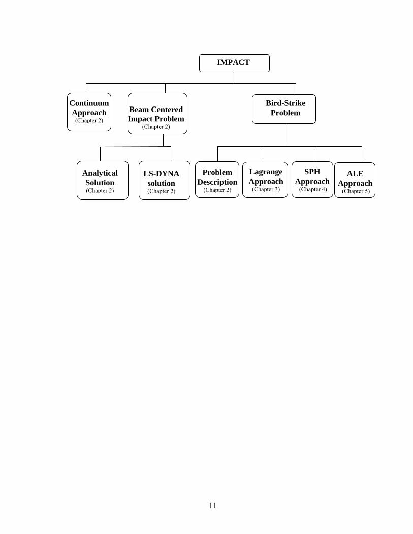
1.3 Outline of the Thesis
We first include in Chapter 2 a description of the impact problem summarizing the
continuum approach used for soft body impact events. A simple supported beam example
was solved analytically and contrasted to LS-DYNA simulations. Also the description of the
bird-strike problem, the literature test data used for this work and a general model used for
the bird are shown in Chapter 2. Then the pre-processing, processing and post-processing of
the modeled bird-strike event in LS-DYNA using the Lagrange method is developed in
Chapter 3. Then on Chapter 4 is discussed the Smooth Particle Hydrodynamics (SPH)
formulation, the LS-DYNA capabilities and simulations of the bird-strike using the SPH
formulation. In addition this chapter presents the comparison with the current Lagrangian
model. Chapter 5 deals with the modeling and simulation of the bird-strike using Arbitrary
Lagrange Eulerian (ALE) formulation and its comparison to the Lagrangian and SPH
simulation. Conclusions are presented in Chapter 6.
11
Analytical Solution (Chapter 2)
LS-DYNA solution (Chapter 2)
Problem Description
(Chapter 2)
LagrangeApproach
(Chapter 3)
SPH Approach (Chapter 4)
ALE Approach
(Chapter 5)
IMPACT
Continuum Approach
(Chapter 2)
Beam Centered Impact Problem
(Chapter 2)
Bird-Strike Problem

12
Chapter 2. Impact Analysis
When we talk about the bird-strike event in this work we are referring to the impact
of a bird against an aircraft component. The bird-strike events are considered as soft body
impact in structural analysis because the yield point of the bird is far smaller when compared
with that of the target. Thus, the bird at the impact can be considered as a fluid material. The
soft body impact results in damage over a larger area if compared with ballistic impacts.
Now, to better understand, bird-strike events let us first understand the impact problem and
then apply it to the bird-strike event being studied in this work.
2.1 A Continuum Approach
Let us begin by discussing the continuum approach used to solve the soft body impact
problem. There major equations are solved by LS-DYNA to obtain the velocity, density, and
pressure of the fluid for a specific position and time. These equations are: conservation of
mass, conservation of momentum, and constitutive relationship of the material. The most
important information in an impact analysis is the pressure generated by the body on the
target. Thus, we proceed to explain the basic equations used to find the pressure generated at
the beginning of the impact as developed in Cassenti (1979).

13
2.1.1 Governing Equations Let us begin with the general form of the conservation of momentum, which can be stated as
follows:
( )DtρD Vbσ =+⋅∇ ρ (2.1)
where σ is the stress matrix, b the body forces per unit mass, ρ the density, and V the
velocity vector. For the impact problem, no body forces are considered: thus, 0=b . Further,
it is assumed that for equilibrium the normal compressive stress acting in the contact
interface balance the normal pressure exerted for the body over the target within the contact
area. Also, it is assumed that the shear stresses are neglected. Thus, the stress tensor can be
expressed as follows
Pσ −= (2.2)
where P is a diagonal matrix containing only normal pressure components. Thus, the
conservation of momentum becomes
( )DtρD VP =⋅∇− (2.3)
Shear stresses are neglected, and thus Eq. (2.3) may be expanded for the three orthogonal
directions x1, x2 and x3 as follows
x1 direction: ⎟⎟⎠
⎞⎜⎜⎝
⎛∂∂
+∂∂
+∂∂
+∂∂
=∂∂
−3211
ρxuw
xuv
xuu
tu
xP11
x2 direction: ⎟⎟⎠
⎞⎜⎜⎝
⎛∂∂
+∂∂
+∂∂
+∂∂
=∂∂
−3212 xvw
xvv
xvu
tvρ
xP22

14
x3 direction: ⎟⎟⎠
⎞⎜⎜⎝
⎛∂∂
+∂∂
+∂∂
+∂∂
=∂∂
−3213 x
wwxwv
xwu
twρ
xP33
where u, v and w are the velocities in the x1, x2 and x3 directions. The unknowns are the
pressure, the velocity and the density of the body.
The second equation used in the analysis is the conservation of mass and it is written as per
unit volume as follows:
0=⋅∇+ Vρρ
DtD
(2.4)
Equation (2.4) is expanded as follows:
0ρρρρρ
321321=⎟⎟
⎠
⎞⎜⎜⎝
⎛∂∂
+∂∂
+∂∂
+∂∂
+∂∂
+∂∂
+∂∂
−xw
xv
xu
xw
xv
xu
t
Equations (2.3) and (2.4) consist of four independent equations involving seven unknowns.
The unknowns are three components of the pressure P11, P22 and P33, three velocities u, v and
w; and the density ρ. A third equation which will relate the pressure and density is the
constitutive relationship. This reduces the seven unknowns to five and the system of
equations can be solved. For this work different materials are used to model the impact
analysis. The material model will depend on the three different methods used here:
Lagrangian, Smooth Particle Hydrodynamic and Arbitrary Lagrange Eulerian. The
corresponding constitutive equations or equations of state used for each method are discussed
in the next section. However, we can express constitutive relation in its general form as
follows:
)(ρPP = (2.5)

15
Now, the substitution of Eq. (2.5) into Eq. (2.3) leads to:
DtD )()( VP ρ
ρ =⋅∇− → ( ) 0ρ
)(=∇⋅
∂∂
+ ρDtρD PV
(2.6)
To better understand this coupling, let us consider a one-dimensional soft body impact. This
case is representative of the work done in this thesis. Figure 2.1 shows the one-dimensional
soft body impact against a rigid plate in which a compressive shock wave propagates at
speed v through the fluid. The pressure corresponding to the zone between the impact surface
and the shock wave is commonly known as Hugoniot pressure. The fluid will move in this
zone with zero velocity and will have an increased density. Equation (2.3) of the one-
dimensional conservation of momentum simplifies to
11 xP
xuu
tuρ xx
∂∂
−=⎟⎟⎠
⎞⎜⎜⎝
⎛∂∂
+∂∂
(2.7)
where P11 is the pressure inside the impact body in the x1 direction, t is the time and x1 is the
distance from the surface.
The conservation of mass, Eq. (2.4), simplifies to
11ρρ
xu
xP
ut
xx∂∂
−=∂∂
+∂∂
(2.8)

16
Figure 2.1: Pressure evaluation model
For a one-dimensional case there are three unknowns: the velocity u, the pressure Pxx, and
the density ρ. Now, Eq. (2.5) is simplified by using a constitutive relation in which the
hydrostatic pressure is expressed as a function of the density:
)ρ(xxxx PP = (2.9)
and the substitution of Eq. (2.9) into Eq. (2.7) leads to
0ρ)ρ('11=
∂∂
+⎟⎟⎠
⎞⎜⎜⎝
⎛∂∂
+∂∂
xP
xuu
tuρ xx (2.10)
where
ρ)ρ('
ddP
P xxxx = (2.11)
Soft body model
u = uo p = po ρ = ρo c = co
u = 0 p = ph ρ = ρh c = ch
Target
X1
x1
vS

17
Equations (2.8) and (2.10) will be used to solve the two unknown density and speed. From
Fig. 2.1 it can be observed that an additional X1 coordinate is included. The fluid included in
the region where X1 is greater than zero has not been affected by the impact, however in the
region where X1 is less than zero the pressure and density are higher than the nominal values.
The shock wave is located in the fluid at a distance of:
tvx S ⋅=1 (2.12)
where, vS is the propagation velocity of the shock front. The coordinate X1, that is the same as
the distance from the front shock, can be expressed as:
tvxX S ⋅−= 11 (2.13)
Let U be the fluid speed in the reference X1. The fluid velocity can then be expressed as
SvUu += (2.14)
Both the density ρ and the velocity U are function of the coordinate X1 as shown in Eqs.
(2.15) and (2.16).
)( 1XUU = (2.15)
)( 1Xρρ = (2.16)
Substituting Eqs. (2.14), (2.15) and (2.16) in Eq. (2.8) results in:
1CρU = (2.17)
Substituting Eqs. (2.14), (2.15) and (2.16) in Eq. (2.10) results in:
22 )(ρ
21 CρPU =+ (2.18)
where C1 and C2 are constants and
18
∫= dρρρP
ρP xx )(')( (2.19)
The constants C1 and C2 can be obtained considering the region beyond the shock front
where:
So vuU −−= (2.20)
oρρ = (2.21)
The nominal speed uo is in the negative X1 direction. Substituting Eqs. (2.20) and (2.21) into
Eqs. (2.17) and (2.18) defines C1 and C2. Thus, Eqs. (2.17) and (2.18) become:
( ) ( )oSo ρPvuρPρU ++=+ 2221)ρ(
21
(2.22)
( )Soo vuρρU +−= (2.23)
Also for the region between the shock front and the surface of impact:
SvU −= (2.24)
hρρ = (2.25)
Substituting Eqs. (2.24) and (2.25) into Eq. (2.23) results in:
⎟⎟⎠
⎞⎜⎜⎝
⎛+=
S
oo v
uρρ 1h (2.26)
Substituting Eqs. (2.24) thru (2.26) in Eq. (2.22) results in one equation (Eq. 2.27) in which
the only unknown is the front propagation speed, vS.
( ) ( )oSoS
ooS ρPvu
vu
ρPv ++=⎥⎥⎦
⎤
⎢⎢⎣
⎡⎟⎟⎠
⎞⎜⎜⎝
⎛++ 22
211
21
ρρ (2.27)

19
Then Eq. (2.27) is solved for vS. Note that ρh is found from Eq. (2.26) and the corresponding
Hugoniot pressure, ph is found using Eq. (2.9). The Hugoniot pressure is that corresponding
to the peak pressure generated at the beginning of the impact and different finite element
formulations will be used to compute this pressure. The normal stress generated in the
structure of the target will be equal to the Hugoniot pressure at the beginning of the impact as
depicted in Fig. 2.2.
Figure 2.2: Pressure evaluation model
The next sections will include a brief discussion of the different methods used for the
solution of the bird-strike equations discussed before using LS-DYNA. First the current
Lagrangian formulation will be discussed followed by the two new methods studied in this
work, the Arbitrary Lagrange Eulerian (ALE) method and the Smooth Particle
Hydrodynamic (SPH) method.
σ = ph
vs
Soft Body
p = ph
Target

20
Initial Position (t = 0) Final Position (t = tf)
2.1.2 Lagrangian Approach
The various formulations existent for the finite element analysis differ in the
reference coordinates used to describe the motion and the governing equations. The
Lagrangian method uses material coordinates (also known as Lagrangian coordinates) as the
reference; these coordinates are generally denoted as X. The nodes of the Lagrangian mesh
are associated to particles in the material under examination; therefore, each node of the
mesh follows an individual particle in motion, this can be observed in Fig. 2.3. This
formulation is used mostly to describe solid materials. The imposition of boundary
conditions is simplified since the boundary nodes remain on the material boundary. Another
advantage of the Lagrangian method is the ability to easily track history dependant materials.
The main disadvantage of the Lagrangian method is the possibility of inaccurate results and
the need of remeshing due to mesh deformations. Since in this method the material moves
with the mesh, if the material suffers large deformations as observed in Fig. 2.4, the mesh
will also suffer equal deformation and this leads to inaccurate results.
Figure 2.3: Lagrangian mesh.
NodesMaterial Particles

21
Initial Material Deformed Material
Nodal Points
Material Points
Figure 2.4: Example of Lagrangian mesh deformation
Material Domain (RM) Spatial Domain (RS)
φ (X, t)
X x
Figure 2.5: Description of motion for Lagrange formulation

22
The reference coordinates for the Lagrange method are the material coordinates, X. Let us
define RM as the material domain (reference for the Lagrangian domain) and RS as the
spatial domain. The motion description for the Lagrangian formulation is:
x = φ(X, t) (2.28)
where φ(X, t) is the mapping between the current position and the initial position, as shown in
Fig. 2.5.
The displacement u of a material point is defined as the difference between the current
position and the initial position:
u(X, t) = φ (X, t) – X = x – X (2.29)
To minimize the mesh deformations present in the Lagrangian meshes, two formulations
exist. The first formulation is known as the Updated Lagrangian (UL) formulation, where the
desired quantities are calculated with respect to the referential coordinates (X) for each time
step. At the end of the time step, the referential coordinates are updated. In other words, the
new reference is the current state. This formulation is expressed in terms of Eulerian
measures of stress and strain. The derivatives and integrals for this formulation are with
respect to the Eulerian (spatial) coordinates x.
The second formulation is known as the Total Lagrangian (TL) formulation, which is in
terms of the Lagrangian measures of stress and strains. The derivatives and integrals of this
formulation are with respect to the material coordinates X. Unlike the UL formulation, the
reference for the TL formulation is the initial state, when t = 0.
23
Two type of materials were used for the bird model: material null and the elastic fluid. The
material null considers a fluid material composed of 90% of water and 10% of air. This
material allows consider equation of state without computing deviatoric stresses. The
equation of state used with this material was the equation of state tabulated. This equation of
state defines the pressure P as follows
( ) ( )EVV εγε TCP +=
where C represents the constant array and T the temperature constants that depends on the
volumetric strain. For the type of impact problems studied in this work, temperature does not
play a big role. In this context, the term γT(εV)E vanishes because T(εV) is zero and thus the
equation of state becomes as follows
( )VεCP = (2.30)
The volumetric strain εV is given by the natural logarithm of the relative volume. The elastic
fluid material was also used for the Lagrangian model. This material is described in the next
section with details.
In the Lagrangian simulations performed in this work, Eq. (2.30) is expressed in terms of the
constitutive equation expressed in Eq. (2.5), and needs to solve for velocities, density and
pressure of the problem of impact. Figure 2.6 shows an example of the deformation obtained
during the impact using a Lagrange model of the soft body.
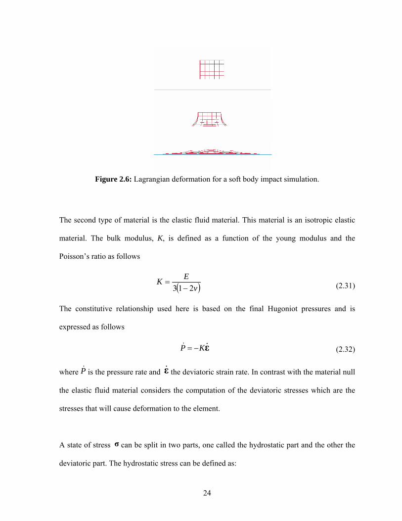
24
Figure 2.6: Lagrangian deformation for a soft body impact simulation.
The second type of material is the elastic fluid material. This material is an isotropic elastic
material. The bulk modulus, K, is defined as a function of the young modulus and the
Poisson’s ratio as follows
( )vEK
213 −= (2.31)
The constitutive relationship used here is based on the final Hugoniot pressures and is
expressed as follows
εKP −= (2.32)
where P is the pressure rate and ε the deviatoric strain rate. In contrast with the material null
the elastic fluid material considers the computation of the deviatoric stresses which are the
stresses that will cause deformation to the element.
A state of stress σ can be split in two parts, one called the hydrostatic part and the other the
deviatoric part. The hydrostatic stress can be defined as:
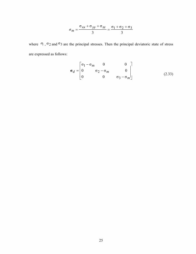
25
3σσσ
3σσσ 321 ++
=++
= zzyyxxmσ
where 1σ , 2σ and 3σ are the principal stresses. Then the principal deviatoric state of stress
are expressed as follows:
⎥⎥⎥
⎦
⎤
⎢⎢⎢
⎣
⎡
−−
−=
m
m
m
dσσ000σσ000σσ
3
2
1σ
(2.33)
26
2.1.3 ALE Approach
Eulerian Formulation
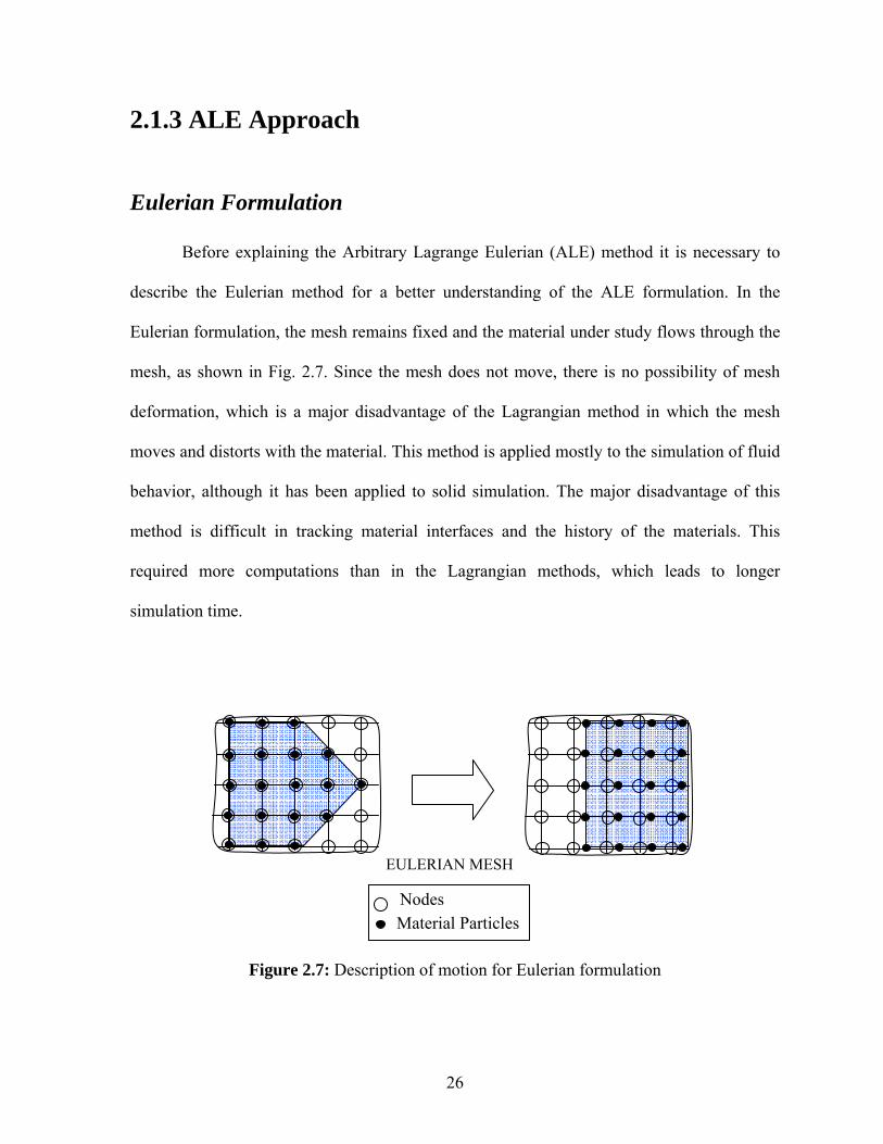
Before explaining the Arbitrary Lagrange Eulerian (ALE) method it is necessary to
describe the Eulerian method for a better understanding of the ALE formulation. In the
Eulerian formulation, the mesh remains fixed and the material under study flows through the
mesh, as shown in Fig. 2.7. Since the mesh does not move, there is no possibility of mesh
deformation, which is a major disadvantage of the Lagrangian method in which the mesh
moves and distorts with the material. This method is applied mostly to the simulation of fluid
behavior, although it has been applied to solid simulation. The major disadvantage of this
method is difficult in tracking material interfaces and the history of the materials. This
required more computations than in the Lagrangian methods, which leads to longer
simulation time.
Figure 2.7: Description of motion for Eulerian formulation
EULERIAN MESH
Nodes Material Particles

27
Material Domain (RM) Spatial Domain (RS)
φ -1 (x, t)
Figure 2.8: Mapping between the material and the spatial domain for an Eulerian description.
The Eulerian motion description can be expressed as an inverse map of the Lagrangian
motion as in Eq. (2.34). Figure 2.8 shows the mapping between the material and spatial
domain for the Eulerian method. This method expresses the material coordinates in terms of
the spatial coordinates as follows:
X = φ-1 (x, t) (2.34)
ALE Approach
The Arbitrary Lagrange-Eulerian (ALE) formulation is a combination of the
Lagrange and Eulerian formulations in which the reference is set arbitrarily by the user in
order to capture the advantages of the methods while minimizing the disadvantages, as
shown in Fig. 2.9. The user must set the mesh motion that best suite the problem in order to
minimize the mesh distortions and obtain the best results. This is the main disadvantage of
the method, is that the user must be experienced in order to select the best method, and
interpret the results obtained.
X x
28
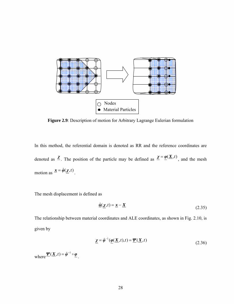
Figure 2.9: Description of motion for Arbitrary Lagrange Eulerian formulation
In this method, the referential domain is denoted as RR and the reference coordinates are
denoted as χ . The position of the particle may be defined as ),( tXφχ = , and the mesh
motion as ),(ˆ tχφx = .
The mesh displacement is defined as
Xxχu −=),(ˆ t (2.35)
The relationship between material coordinates and ALE coordinates, as shown in Fig. 2.10, is
given by
),()),,((ˆ 1 ttt XΨXφφχ == −
(2.36)
where φφXΨ 1ˆ),( −=t .
Nodes Material Particles

29
Material Domain (RM) Spatial Domain (RS)
Ψ=ϕϕ ˆ),( tX X x
Ψ (X, t) Referential Domain (RR) Ψt ϕϕ =),(ˆ χ
Figure 2.10: Maps between material, spatial and referential domains.
Figure 2.11 shows how an ALE simulated soft body interacts with a rigid plate. Instead of
defining a contact between the target and the soft body a coupling occurs in which the loads
are computed as a function of the penetration of the soft body in the target. The material used
for the ALE bird was the elastic fluid material, previously explained.
Figure 2.11: Soft body impact using ALE.
χ
30
2.1.4 SPH Formulation
Smooth Particle Hydrodynamics (SPH) formulation is a meshless Lagrangian
technique used to model the fluid equations of motion using a pseudo-particle interpolation
method to compute smooth hydrodynamic variables. Initially this method was used to
simulate astrophysical phenomenon, but recently it has been used to resolve other physics
problems in continuum mechanics, crash simulations, brittle and ductile fracture in solids.
Due to the absence of a grid, this method allows solving many problems that are hardly
reproducible in other classical methods discarding the problem of large mesh deformations or
tangling. Another advantage of the SPH method is that due to the absence of a mesh,
problems with irregular geometry can be solved.
In this formulation, the fluid is represented as a set of moving particles, each one
representing an interpolation point, where all the fluid properties are known. Then, with a
regular interpolation function called smoothing length the solution of the desired quantities
can be calculated for all the particles.
A real fluid can be modeled as many fluid particles provided that the particles are small
compared to the scale over which macroscopic properties of the fluid varies, but large
enough to contain many molecules so macroscopic properties can be defined sensibly. A
large number of particles are needed for the SPH calculations, since the continuum limit is
recovered when the number of particles goes to infinity.
31
Particles in the SPH method carry information about their hydrodynamic and thermodynamic
information, this in addition to the mass needed to specify the evolution of the fluid. Nodes in
SPH are similar to nodes in a mesh, the difference is that these nodes are continuously
deformable and distort automatically to put more of the computational effort in regions of
relatively high density.
One disadvantage in SPH is that this method is computationally demanding, both in memory
and in CPU time. This can be overcome using a parallel analysis with more than one CPU.
There is also the difficulty of establishing the boundary condition when using the SPH
method. Another disadvantage is that particles may penetrate the boundaries and causing loss
of smoothness and accuracy.
The moving particles are described by
( ) ( )( ) Piii tmtx ∈, (2.37)
where P is the set of moving particles, xi(t) the location of particle i, and mi(t) the weight of
the particle. Lacome (2001) presented the movement of each particle and the change of the
weight, given by
( ) iii mtx
dtdm
,V⋅∇= (2.38)
The quadrature formula can be written as:
( ) ( ) ( )( )∫ ∑
Ω ∈
≈
Pjjj txftmdxxf
(2.39)

32
⎪⎪⎪
⎩
⎪⎪⎪
⎨
⎧
≥
≤≤−
≤+−
×=
2yfor0
2y1for)y2(41
1yfory43y
231
)y( 3
32
1αθ
⎟⎟⎠
⎞⎜⎜⎝
⎛ −=−
hxx
hhxxW ji
ji θ1),(
A useful concept in SPH is the smoothing kernel. It is necessary first to introduce the
auxiliary cubic B-spline function which has some good properties of regularity.
(2.40)
Where, α1 is a constant that depends on de dimension and the shape of the kernel function. In
two dimensions:
πα
710
1 = (2.41)
Lacome (2001) also suggested the smoothing kernel as:
(2.42)
where h is the smoothing length of the kernel. Generally, a property A(xi) is represented by
its smooth particle approximation Ah(xi) of the function, and by approximating the integral in
Eq. (2.39):
( ) ( )( ) ( )∑
=
−=N
jji
j
jji
h hWxxA
mx1
,xxAρ (2.43)
The gradient of the function is obtained by applying the operator of derivation on the
smoothing length.

33
( ) ( )( ) ( )∑
=
−∇=∇N
jji
j
jji
h hWxxA
mx1
,ρ
xxA (2.44)
Initially in the SPH method, the smoothing length was chosen as constant during the entire
simulation. However, it was shown that it is better for each particle to have its own
smoothing length, depending on the local number of particles. The current method used for
the smoothing length is the gather formulation. In this method,
)h(xh i=
is defined and the neighboring particles of a defined particle are the particles inside of a
sphere centered in xi with a radius of h(xi).
The equations for the SPH formulation presented in this section have been described by
Monaghan (1989). The mass density has been defined as
( ) ( )∑=
−=N
jjij hWmx
1
,xxρ (2.45)

34
The equation of conservation of the mass in a Lagrangian form is:
( ) Vx ∇−= ρρ
idtd
(2.46)
The SPH approximation for the conservation of mass can be written in two different ways:
( ) ( ) ( )( ) ij
N
jijji Wxxm
dtd
∇−=∑=1
ρ vvx (2.47)
or
( ) ( )( ) ij
N
jj
jji Wxm
dtd
∇=∑=1
ρρρ vx
(2.48)
The SPH momentum equation may be written as:
( ) ( ) ( )∑=
⎟⎟⎟
⎠
⎞
⎜⎜⎜
⎝
⎛∇−∇=
N
jji
j
jij
i
iji W
xPW
xPm
dtd
122 ρρ
xv (2.49)
Figure 2.12: Integration cycle in time of the SPH computation process.
Velocity/position LS-DYNA
Smoothing length SPH
Neighbor
Density, strain
Pressure, energy, stresses LS-DYNA
Particles Forces SPH
Contact, boundary
Acceleration

35
Figure 2.12 illustrates an integration cycle in time of the SPH computation process Lacome,
(2001). In the SPH analysis, it is important to know which particle will interact with its
neighbors because the interpolation depends on these interactions. Therefore, a neighboring
search technique has been developed Lacome (2001). The influence of a particle is
established inside of a sphere of radius of 2h, where h is the smoothing length. In the
neighboring search, it is also important to list, for each time step, the particles that are inside
that sphere. If we have N particles, then it is required (N-1) distance comparison. If this
comparison is done for each particle, then the total amount of comparisons will be N (N-1).
For the neighboring search, the bucket sort algorithm is used. The domain covered by the
particles is split in several boxes of a given size. First the algorithm searches for neighbors,
for each particle inside the main box and the neighbor boxes contained in the domain of
influence of the particle. A scheme of this neighbor search is shown in Fig. 2.13 (Lacome,
2001).
It is better to have a variable smoothing length to avoid problems related with expansion and
compression of material. The concept of a variable smoothing length was developed by W.
Benz. The main idea of this concept is that it is necessary to keep enough particles in the
neighborhood to validate the approximation of continuum variables. The smoothing is
allowed to vary in time and space. For a constant smoothing length, a material expansion can
lead to numerical fracture and a material compression can slow down the calculation
significantly.

36
Figure 2.13: Neighbor search particles inside a 2h radius sphere.
The time rate of change for the smoothing length is given by the following equation:
V⋅∇= hdtdh
31
(2.50)
The mass has to be kept constant in the neighborhood to achieve this equation. The total
mass of n particles inside a sphere of radius 2h is:
( ) 3834 hnVnmnM πρρ ⋅⋅=⋅=⋅=
Then we have the time rate of change of the mass:
dtdhnhn
dtdM 3
33
32π3
32dtdρ
πρ+⋅⋅=
Since the mass is constant in time, the left hand of the equation is equal to zero. Thus the
equation is simplified to:
V⋅∇= hdtdh
31
(2.51)

37
Due to computational efficiency a minimum of 0.2 times the initial smoothing length and a
maximum value for the smoothing length twice the initial smoothing length are required. The
value of the smoothing length is then between those minimum and maximum values.
The same example for soft body impact developed using Lagrange and ALE was solved
using SPH method. The material type and the definition of the contact used in SPH were the
same as in the Lagrange case. Figure 2.14 shows an example of the deformation obtained
during the impact using a Lagrange model of the soft body.
Figure 2.14: SPH simulation for a soft body impact.

38
2.2 Beam Centered Impact Problem Before studying bird-strike events, we proceeded to solve a beam centered impact
problem (Goyal and Huertas, 2006c). The problem consisted in taking a simply supported
beam of length, L, of 100 mm over which a rigid object of mass, mA, of 2.233 × 10⁻³ kg
impacts at a constant initial velocity of, (vA)1, 100 m/s. The beam has a solid squared cross
section of length 4 mm, modulus of elasticity, EB, of 205 GPa, and a density, ρB, of 3,925
kg/m3. Figure 2.15 shows a schematic of the problem. The goal of this problem is to obtain
the pressure maximum peak pressure exerted at the moment of impact. The problem is solve
analytically and then compared to the corresponding outputs from LS-DYNA for the
Lagrange, SPH, and ALE, methods.
Figure 2.15: Beam impact problem.
(vA)1
L=100 mm
A
B
L/2 L/2
A
5 mm
5 mm
5 mm
4 mm
4 mm ρB EB
ρA EA
Projectile dimensions

39
2.2.1 Analytical solution
Figure 2.16: Beam impact problem simplification.
Since the impact occurs at only one point, the problem can be solved by concentrating all the
mass of the beam at the point of impact, i.e., at the center of the beam. Thus will simply the
problem to a problem of central impact between two masses, as shown in Fig. 2.16.
The solution is a split in two stages. The first stage is the impact between the two masses
with its respective initial velocities. At this stage an impact force occurs in the beam that is
exactly the same as that generated by the beam against the projectile. The second stage is
when both masses stick together with a common velocity, experiencing a perfectly plastic
impact. In other words the coefficient of restitution for this problem is considered as e=0.
This coefficient of restitution may be expressed as:
( ) ( )( ) ( )11
22
AB
ABvvvv
e−
−= (2.52)
(vA)1A
L/2 L/2
B(vB)1=0
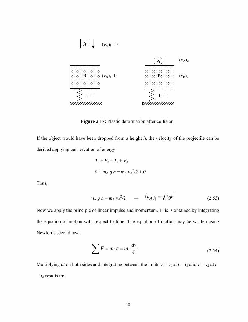
40
Figure 2.17: Plastic deformation after collision.
If the object would have been dropped from a height h, the velocity of the projectile can be
derived applying conservation of energy:
To + Vo = T1 + V2
0 + mA g h = mA vA2/2 + 0
Thus,
mA g h = mA vA2/2 → ( ) ghvA 21 = (2.53)
Now we apply the principle of linear impulse and momentum. This is obtained by integrating
the equation of motion with respect to time. The equation of motion may be written using
Newton’s second law:
dtdvmamF ⋅=⋅=∑ (2.54)
Multiplying dt on both sides and integrating between the limits v = v1 at t = t1 and v = v2 at t
= t2 results in:
A (vA)1= u
(vB)1=0B B
A (vA)2
(vB)2
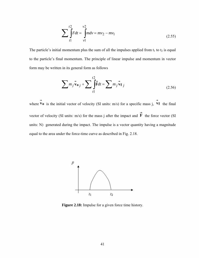
41
12
2
1
2
1
mvmvmdvFdtv
v
t
t
−== ∫∑∫ (2.55)
The particle’s initial momentum plus the sum of all the impulses applied from t1 to t2 is equal
to the particle’s final momentum. The principle of linear impulse and momentum in vector
form may be written in its general form as follows
∑ ∑∫∑ =+ jj
t
t
jj mdtm fo vFv2
1 (2.56)
where ov is the initial vector of velocity (SI units: m/s) for a specific mass j, fv the final
vector of velocity (SI units: m/s) for the mass j after the impact and F the force vector (SI
units: N) generated during the impact. The impulse is a vector quantity having a magnitude
equal to the area under the force-time curve as described in Fig. 2.18.
Figure 2.18: Impulse for a given force time history.
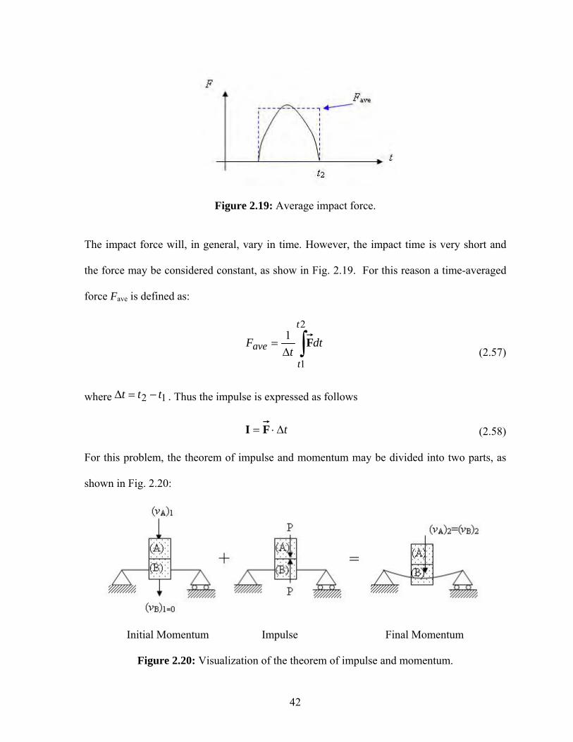
42
Figure 2.19: Average impact force.
The impact force will, in general, vary in time. However, the impact time is very short and
the force may be considered constant, as show in Fig. 2.19. For this reason a time-averaged
force Fave is defined as:
∫∆=
2
1
1t
t
ave dtt
F F (2.57)
where 12 ttt −=∆ . Thus the impulse is expressed as follows
t∆⋅= FI (2.58)
For this problem, the theorem of impulse and momentum may be divided into two parts, as
shown in Fig. 2.20:
Initial Momentum Impulse Final Momentum
Figure 2.20: Visualization of the theorem of impulse and momentum.

43
The diagrams indicate direction and magnitude of the particle’s initial and final momentum.
The particle’s initial momentum plus the sum of all the impulses applied from t1 to t2 is equal
to the particle’s final momentum.
( ) ( )∑ ∑∫∑ =+ 2
01 jj
t
jj vmdtvm F (2.59)
where the sub-indices 1 and 2 correspond for the instants before and after the impact
respectively. For our problem:
( ) ( )21 )(00 ABAAA vmmvm ⋅+=++ (2.60)
The final velocity of the projectile A and that of the concentrated mass of the beam B will be
the same after the impact because a restitution coefficient of zero was assumed for this
problem. Then this final velocity can be calculated as:
( ) ( ) ( )12 ABA
AA v
mmm
v ⋅+
= (2.61)
Now, as a consequence of concentrating all the mass at the center of the beam, the model is
similar to that of a one degree of freedom damped vibrating system, as shown in Fig. 2.21.
The principle of impulse and momentum for the system described in Fig. 2.21 is written as:
( )2000
)()( ABA
ttt
vmmdtuckudtdttFooo
⋅+=−− ∫∫∫ (2.62)
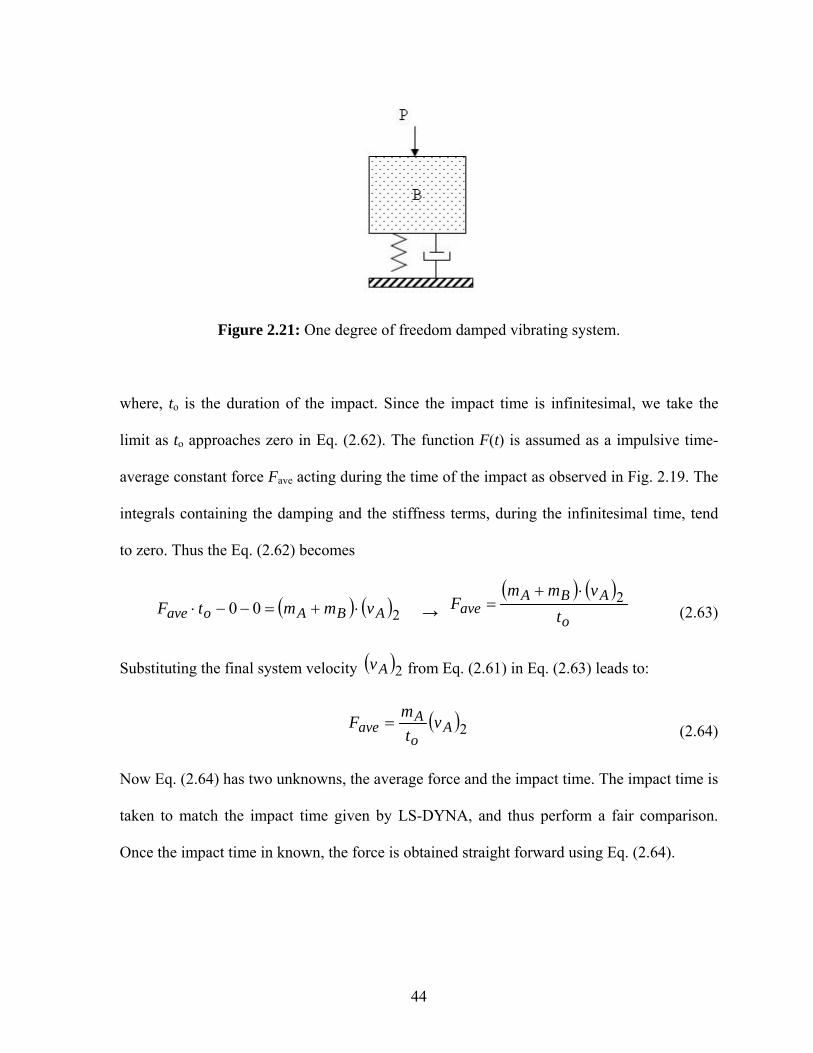
44
Figure 2.21: One degree of freedom damped vibrating system.
where, to is the duration of the impact. Since the impact time is infinitesimal, we take the
limit as to approaches zero in Eq. (2.62). The function F(t) is assumed as a impulsive time-
average constant force Fave acting during the time of the impact as observed in Fig. 2.19. The
integrals containing the damping and the stiffness terms, during the infinitesimal time, tend
to zero. Thus the Eq. (2.62) becomes
( ) ( )200 ABAoave vmmtF ⋅+=−−⋅ → ( ) ( )
o
ABAave t
vmmF 2⋅+
= (2.63)
Substituting the final system velocity ( )2Av from Eq. (2.61) in Eq. (2.63) leads to:
( )2Ao
Aave v
tm
F = (2.64)
Now Eq. (2.64) has two unknowns, the average force and the impact time. The impact time is
taken to match the impact time given by LS-DYNA, and thus perform a fair comparison.
Once the impact time in known, the force is obtained straight forward using Eq. (2.64).
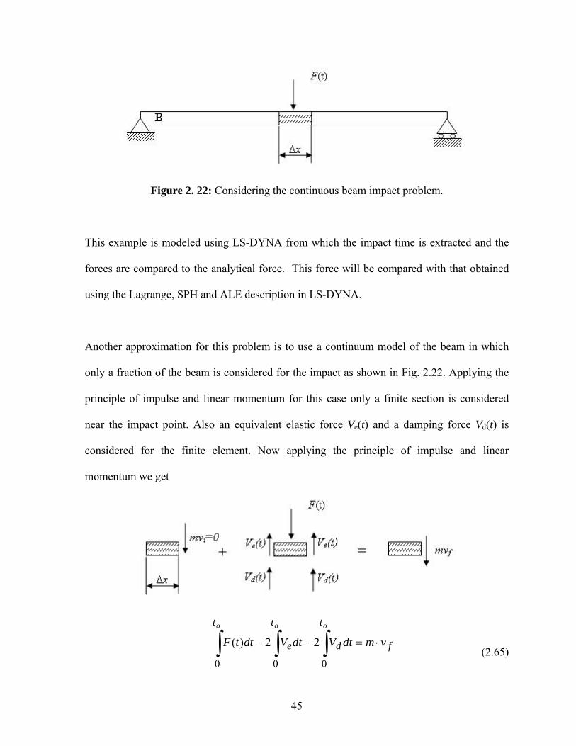
45
Figure 2. 22: Considering the continuous beam impact problem.
This example is modeled using LS-DYNA from which the impact time is extracted and the
forces are compared to the analytical force. This force will be compared with that obtained
using the Lagrange, SPH and ALE description in LS-DYNA.
Another approximation for this problem is to use a continuum model of the beam in which
only a fraction of the beam is considered for the impact as shown in Fig. 2.22. Applying the
principle of impulse and linear momentum for this case only a finite section is considered
near the impact point. Also an equivalent elastic force Ve(t) and a damping force Vd(t) is
considered for the finite element. Now applying the principle of impulse and linear
momentum we get
f
t
d
t
e
t
vmdtVdtVdttFooo
⋅=−− ∫∫∫000
22)( (2.65)
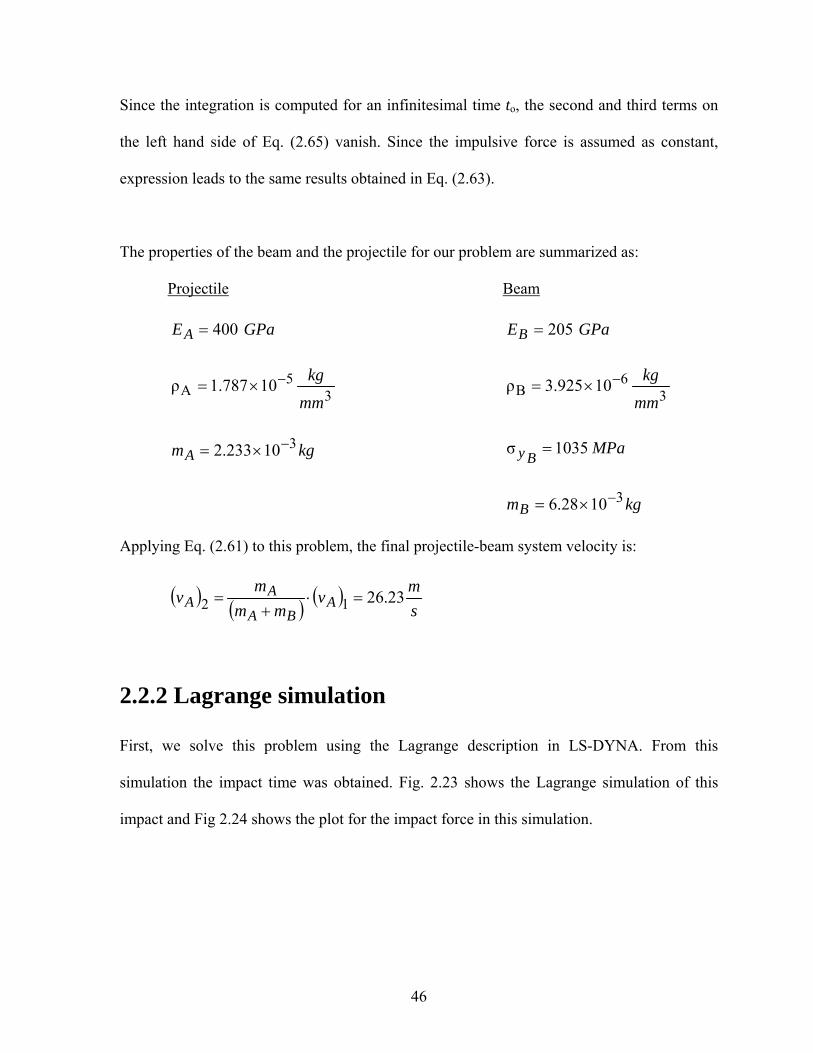
46
Since the integration is computed for an infinitesimal time to, the second and third terms on
the left hand side of Eq. (2.65) vanish. Since the impulsive force is assumed as constant,
expression leads to the same results obtained in Eq. (2.63).
The properties of the beam and the projectile for our problem are summarized as:
Projectile Beam
GPaEA 400= GPaEB 205=
35
A 10787.1ρmm
kg−×= 36
B 10925.3ρmm
kg−×=
kgmA310233.2 −×= MPaBy 1035σ =
kgmB31028.6 −×=
Applying Eq. (2.61) to this problem, the final projectile-beam system velocity is:
( ) ( ) ( )sm
vmm
mv A
BA
AA 23.2612 =⋅
+=
2.2.2 Lagrange simulation
First, we solve this problem using the Lagrange description in LS-DYNA. From this
simulation the impact time was obtained. Fig. 2.23 shows the Lagrange simulation of this
impact and Fig 2.24 shows the plot for the impact force in this simulation.

47
Figure 2.23: Lagrange simulation of transversal beam impact
Figure 2.24: Impact force for the Lagrangian simulation
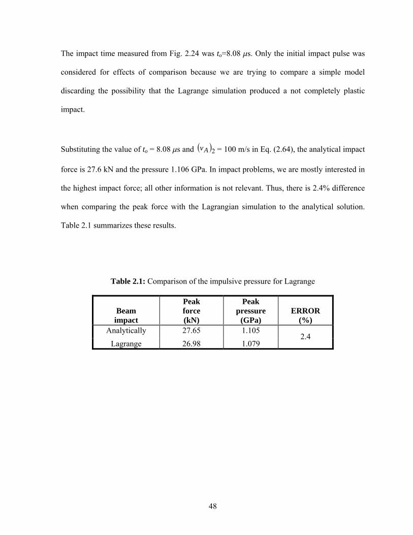
48
The impact time measured from Fig. 2.24 was to=8.08 ms. Only the initial impact pulse was
considered for effects of comparison because we are trying to compare a simple model
discarding the possibility that the Lagrange simulation produced a not completely plastic
impact.
Substituting the value of to = 8.08 ms and ( )2Av = 100 m/s in Eq. (2.64), the analytical impact
force is 27.6 kN and the pressure 1.106 GPa. In impact problems, we are mostly interested in
the highest impact force; all other information is not relevant. Thus, there is 2.4% difference
when comparing the peak force with the Lagrangian simulation to the analytical solution.
Table 2.1 summarizes these results.
Table 2.1: Comparison of the impulsive pressure for Lagrange
Beam impact
Peak force (kN)
Peak pressure
(GPa) ERROR
(%) Analytically 27.65 1.105
Lagrange 26.98 1.079 2.4

49
2.2.3 ALE simulation of the beam centered impact The problem is also solved using the Arbitrary Lagrange Eulerian (ALE) description. The
major challenge in this ALE model is that LS-DYNA does not allow the use of rigid material
for the bird and the creation of a reference void mesh around it. As discussed earlier the
constitutive relation for this material varies from that used in the Lagrange case. Figure 2.25
shows the progression and the deformation obtained in this simulation.
Figure 2.25: ALE simulation of transversal beam impact
The impulse time for this simulation was similar to that obtained using Lagrangian approach
and was to=8.10 ms. Using Eq. (2.65), the analytical impact force was 27.58 kN. The force
plot for the ALE simulation is shown in Fig. 2.26. From the simulation and analytical values
the results are within 6.2%. Table 2.2 summarizes these results.

50
Table 2.2: Comparison of the impulsive pressure for ALE
Beam impact Peak force (kN)
Peak pressure
(GPa) % ERROR Analytically 27.65 1.105
ALE 25.94 1.037 6.2
0
5000
10000
15000
20000
25000
30000
0.00E+00 5.00E-05 1.00E-04 1.50E-04 2.00E-04 2.50E-04
Time (s)
Forc
e (N
)
ALE BEAM
Figure 2.26: Force plot for ALE simulation

51
2.2.4 SPH simulation of the beam centered impact Lastly, the problem is simulated using the SPH formulation. In this case the projectile was
composed of SPH particles. Figure 2.27 shows that the projectile suffered a deformation after
the impact, which may affect the results for the computed impact force.
Figure 2.27: SPH simulation of transversal beam impact
The impulse time was to=8.03 ms. Using this value in Eq. (2.64) the analytical impact force is
found as 29.02 kN and the pressure as 1.161 GPa. From Fig. 2.28 it can be observed that the
peak force in this SPH simulation was 27.84 kN which is 4.06 % lower than the theoretically
value. The comparison for the force and pressure of this case with the analytical solution is
shown in Table 2.3. It should be noted that the results converge to the analytical model. It
was necessary to assign a high value of young modulus to the material of the bird in order to
simulate it as a rigid body.

52
0.00E+00
5.00E+03
1.00E+04
1.50E+04
2.00E+04
2.50E+04
3.00E+04
0.00E+00
5.00E-05 1.00E-04 1.50E-04 2.00E-04 2.50E-04
Time (s)
Forc
e (N
)
SPH beam
Figure 2.28: Force plot for SPH simulation
Table 2.3: Comparison of the impulsive pressure
Beam impact Peak force (kN)
Peak pressure
(GPa) % ERROR Analytically 29.02 1.161
SPH 27.84 1.11 4.06

53
2.3 Bird-Strike Impact Problem
The beam impact problem was based on rigid body impact in which the analytical
load computation is relatively easily taking. The results obtained from this example provided
us confidence in the methods being used and thus we proceeded to analyze the bird-strike
impact problem. The bird-strike impact problem is a soft body impact which is different from
the rigid body impact. It is a soft body impact problem because the bird is deformable and is
composed of fluid and air, and the yield stress is far smaller when compared to that of the
target.
Although the characterization for soft body impact is a complex problem, researchers have
studied this problem using test data. Barber et al. (1975) performed an experimental
characterization of bird-strike events. A bird-strike event may occur in different parts of an
aircraft; however, the scope of this work is to study bird-strike against fan-blades. Figure
2.29(a) shows the damage caused by bird impact on the turbine fan blades. This only shows
us that this problem is crucial and that by predicting the impact pressure will help us design
better fan blades. Furthermore, a fan blade is composed of both flat and tapered sections.
Thus, we focus our attention on analyzing bird-strikes against flat and tapered plate using
Lagrange, SPH and ALE formulations in LS-DYNA. We use the work by Barber et al.
(1975) as a mean of comparison. The results should be within 10% for the simulation to be
useful.

54
(a) (b)
Figure 2.29: Force plot for SPH simulation
Currently, the Lagrange formulation is being used to model bird-strike events in fan blades.
However, some disadvantages were found in the simulation. The main disadvantage of this
was that some element deletions occurs which can cause a loss of accuracy when computing
the impact forces and pressures. For this reason two new finite element formulations are
studied—the Smooth Particle Hydrodynamic (SPH) and the Arbitrary Lagrange Eulerian
(ALE) methods—, in an attempt to create standard procedures.
2.3.1 LS-DYNA for Bird-Strike Events
The work done throughout this research is based on bird-strike simulations using LS-DYNA.
Before we continue, let us briefly explain the advantages, disadvantages and features of this
software. The main advantages of LS-DYNA is that it is one of the most robust programs
currently available when simulating problems of nonlinear loading, which includes fluid-
structure interaction and impact problems. LS-DYNA has the capabilities to stand non-
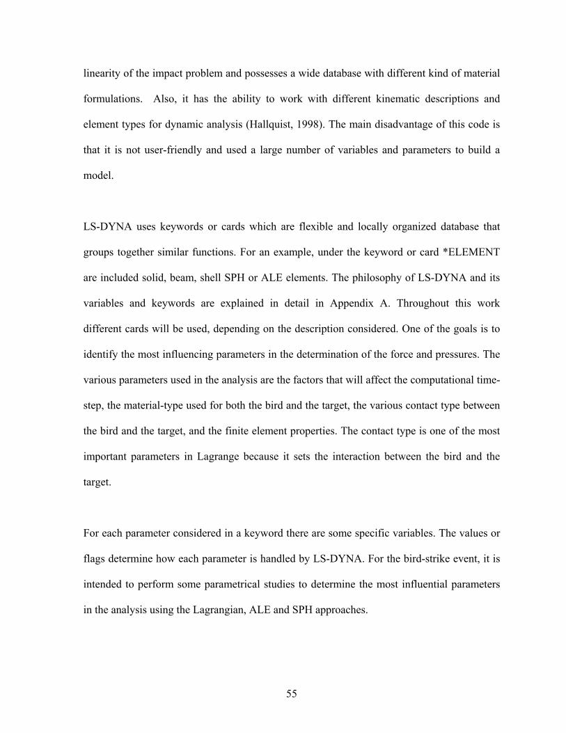
55
linearity of the impact problem and possesses a wide database with different kind of material
formulations. Also, it has the ability to work with different kinematic descriptions and
element types for dynamic analysis (Hallquist, 1998). The main disadvantage of this code is
that it is not user-friendly and used a large number of variables and parameters to build a
model.
LS-DYNA uses keywords or cards which are flexible and locally organized database that
groups together similar functions. For an example, under the keyword or card *ELEMENT
are included solid, beam, shell SPH or ALE elements. The philosophy of LS-DYNA and its
variables and keywords are explained in detail in Appendix A. Throughout this work
different cards will be used, depending on the description considered. One of the goals is to
identify the most influencing parameters in the determination of the force and pressures. The
various parameters used in the analysis are the factors that will affect the computational time-
step, the material-type used for both the bird and the target, the various contact type between
the bird and the target, and the finite element properties. The contact type is one of the most
important parameters in Lagrange because it sets the interaction between the bird and the
target.
For each parameter considered in a keyword there are some specific variables. The values or
flags determine how each parameter is handled by LS-DYNA. For the bird-strike event, it is
intended to perform some parametrical studies to determine the most influential parameters
in the analysis using the Lagrangian, ALE and SPH approaches.

56
2.3.2 General Bird and Target Model Properties
Bird-Model
How to model a bird is quite challenging and a model that best meets the testing bird
properties must be used. The model considered in this work is that of a cylinder, as suggested
by IBRG (2004). It has been shown that this model of bird produce close results to real birds.
In addition, the bird model is assumed isotropic, symmetric and homogeneous. An
approximate aspect ratio (L/D) of 2.03 was used for our bird model. The dimensions vary
depending on the mass of the bird, and are selected from the test data by Barber et al. (1975).
The material properties of the bird were similar to a gelatin material with 90% water and
10% air mixture. It is important to highlight that the mass of the testing birds plays an
important role in the computer simulation because the pressure distribution greatly depends
on the density of the impacting object. Table 2.4 summarizes the main properties used for
modeling the bird.
Table 2.4: Properties for the model of bird
Bird Property: Units
Density 912.61 kg/m3
Pressure Cutoff 0.09974 MPa *Diameter 40 mm
*Length 90 mm
Impact Velocity 198 m/s (442.9 mph) Rigid flat plate
477.4 m/s (1067 mph) Tapered Plate
57
Rigid Flat Plate Target
In this research we use a rigid flat plate target and a deformable tapered plate target. The
purpose of using a rigid flat plate target is to compare the simulations with the experimental
data obtained from Barber et al. (1975). Barber et al. used a rigid flat plate for their
experiments which can be modeled as a circular rigid plate with dimensions of 1 mm
thickness and 15.25 cm of diameter. The material of the target disk was 4340 steel, with a
yield strength of 1035 MPa, Rockwell surface hardness of C45, modulus of elasticity
modulus of 205 GPa, and a Poisson’s ratio of 0.29. These properties of the material will be
used in LS-DYNA to model the flat rigid plate.
The units used for all LS-DYNA simulations are in millimeters for the length, tons for the
mass, seconds for the time, and newtons for the force. All pressure plots will be expressed in
MPa.
Deformable Tapered Plate Target
The deformable tapered plate target properties were taken from the work by Moffat et
al. (2001), who simulated the impacting bird (as a sphere) on a tapered plate using
MSC/DYTRAN software. The properties for the tapered plate are given in Table 2.5.

58
Table 2.5: Tapered plate properties (fixed at the two shortest sides)
Tapered Plate Property: Units
Material Titanium 6-4 plate
Yield Strength 828.0 MPa (1.20091×10⁵ psi)
Modulus of Elasticity 105.0 GPa (15.228×10⁶ psi)
Density 4410 kg/m3 (0.1593 lb/in3)
Poisson ratio 0.31
Effective Length 22.86 cm (9.0 in)
Width 7.62 cm (3.0 in)
Tapered angle 4.0°
Leading edge thickness 0.051 cm (0.0200787 in) Blended uniformly up to 0.160 cm (0.06299 in)
59
2.3.3 Test Data for Bird-Strike Event
The characterization of impacting birds on a rigid plate was done by Barber et al.
(1975). Barber et al. (1975) determined experimentally the pressure-time variations generated
by small birds impacting a flat rigid plate. Barber obtained the pressure data by recording the
output of pressure sensors on the target plate. Barber identified each bird impact with a
specific shot number followed by a letter. The letter indicated the place in the rigid plate at
which the pressure was measured using a transducer. Barber varied the mass of the bird and
the velocity of the bird for each classified shot.
The birds used in the tests (Barber et al., 1975) were of approximately from 70g to 125g, and
were fired at velocities ranging from 60 to 350 m/s (134.2 to 782.9 mph). For a better
simulation of bird-strike events, the density of the bird model is obtained based on the data.
Data Selection
For purposes of this work, we did not run simulations for each test data but for the
data representative of all the experiments put together. Thus, in order to choose the adequate
bird model dimensions and properties used in this work, we created frequency distribution
plots for both the masses and the velocities. Figures 2.30 thru 2.32 summarize this test data
frequency of the bird-strike event provided by Barber et al. (1975).

60
Figure 2.30: Histogram for the bird masses of the Barber et al. (1975) bird impact research.
0
2
4
6
8
10
12
14
16
18
20
50 65 80 95 110 125 140 155 170 185 200 215 230 245 260 275 290 305
Velocity (m/s)
Freq
uenc
y
Figure 2.31: Histogram for the bird velocities of the Barber et al. (1975) bird impact
research.

61
0
5
10
15
20
25
5 10 15 20 25 30 35 40 45 50 55 60 65 70 75 80
Pressure (MN/m2)
Freq
uenc
y
Figure 2.32: Histogram for the bird impact peak pressures of the Barber et al. (1975) bird impact research.
All simulations are based on the data obtained from the histograms in Figs. 2.30 thru 2.32.
We chose the most frequent range of bird masses and velocities. We chose shot 5126A
because it satisfies the chosen bird mass of 0.071 kg and velocity 198 m/s. Thus all flat plate
analysis is based on this particular test data. It is important to highlight that all plots where
reproduced for means of comparison. Now we will explain the procedure how we reproduce
the graphical results of the pressure transducers provided by Barber et al. (1975). These plots
will permit a point to point comparison of the experimental and computer simulation data.
Barber Graph Manipulation
For a fair comparison between the results obtained using LS-DYNA and those
obtained by Barber et al. (1975), we reproduced the experimental data from their tests by
scanning Barber et al. (1975) and scaling them using the MatLab 7.1. As an example, let us
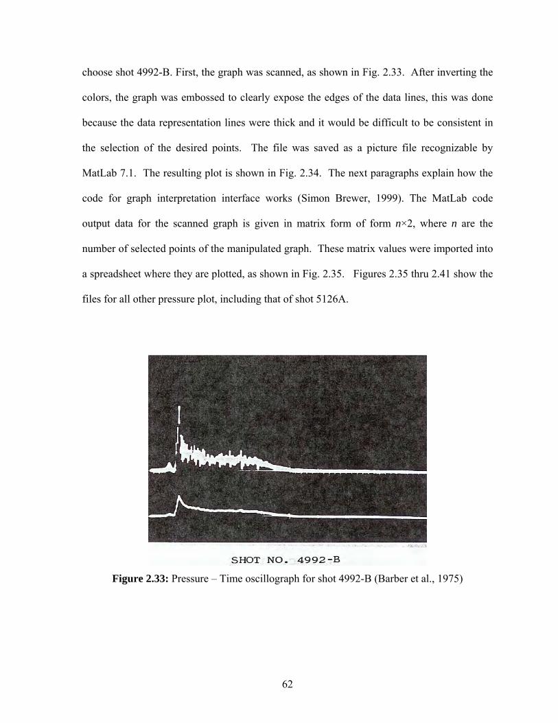
62
choose shot 4992-B. First, the graph was scanned, as shown in Fig. 2.33. After inverting the
colors, the graph was embossed to clearly expose the edges of the data lines, this was done
because the data representation lines were thick and it would be difficult to be consistent in
the selection of the desired points. The file was saved as a picture file recognizable by
MatLab 7.1. The resulting plot is shown in Fig. 2.34. The next paragraphs explain how the
code for graph interpretation interface works (Simon Brewer, 1999). The MatLab code
output data for the scanned graph is given in matrix form of form n×2, where n are the
number of selected points of the manipulated graph. These matrix values were imported into
a spreadsheet where they are plotted, as shown in Fig. 2.35. Figures 2.35 thru 2.41 show the
files for all other pressure plot, including that of shot 5126A.
Figure 2.33: Pressure – Time oscillograph for shot 4992-B (Barber et al., 1975)

63
Figure 2.34: Manipulation of the Pressure- Time oscillograph for shot 4992-B analyzed in
MatLab (Barber et al., 1975)
0
5
10
15
20
25
30
0 50 100 150 200 250 300 350 400 450
Time (10-6 s)
Pres
sure
(MPa
)
Figure 2.35: Pressure vs. time distribution for Shot 4992B (Barber et al., 1975)
Pres
sure
Time
Time
Pres
sure

64
0123456789
0 100 200 300 400 500 600
Time (10-6 s)
Pres
sure
(MPa
)
Figure 2.36: Pressure vs. time distribution for Shot 5181C (Barber et al., 1975)
0
5
10
15
20
25
30
35
40
0 50 100 150 200 250 300 350 400 450
Time (10-6 s)
Pres
sure
(MPa
)
Figure 2.37: Pressure vs. time distribution for Shot 5126A (Barber et al., 1975)

65
0
2
4
6
8
10
12
14
0 50 100 150 200 250 300 350 400
Time (10-6 s)
Pres
sure
(MPa
)
Figure 2.38: Pressure vs. time distribution for Shot 5172C
0
10
20
30
40
50
60
70
0 100 200 300 400 500
Time (10-6 s)
Pres
sure
(MPa
)
Figure 2.39: Pressure vs. time distribution for Shot 5127A

66
0
5
10
15
20
25
30
35
40
0 100 200 300 400 500 600 700
Time (10-6 s)
Pres
sure
(MPa
)
Figure 2.40: Pressure vs. time distribution for Shot 5113A
0
1
2
3
4
5
6
7
8
0 100 200 300 400 500 600
Time (10-6 s)
Pres
sure
(MPa
)
Figure 2.41: Pressure vs. time distribution for Shot 5129A

67
Plots for Bird Impacts on a Rigid Plate
All the approximate data plots show the same behavior and thus we must identify the
stages in the loading observed by Barber et al. (1975). The pressure measured in the test data
shows three different stages as seen in Fig. 2.35 thru 2.41. The first stage, and is the most
important one, is where the peak pressure is generated at the beginning of the impact. The
second stage shows that the bird exerts a steady pressure over the plate and occurs for a short
period of time (150 to 400 µs). In this stage, there are some high frequency variations of the
pressure which influence on the target and will depend in on the geometric characteristic of
the same. The final stage is the fall of the pressure.

68
Chapter 3. Bird-Strike Modeling Based on Lagrangian Formulation
3.1 Lagrangian Bird Model
A Lagrangian approach is used for the bird-strike impact problem. Some of the
typical parameters used to model Lagrangian simulations of bird-strike events are studied in
the following sections. First, we validated the Lagrangian approach with the test data and,
since is the most common technique being used; we use it as a mean of comparison to the
Smooth Particle Hydrodynamics and ALE models.
3.1.1 Pre-processing variables for the Lagrangian model
The definition and meaning of each variables and functions in the various the cards
are described in section A.2. The initial time step scale factor, TSSFAC, inside the
*CONTROL_TIMESTEP card has a default value of 0.9. This value was changed to 0.7 to
avoid contact instabilities. Also the value of the variable ERODE, inside the mentioned card,
was set to 1.0 to allow element erosion when the minimum time-step (TSMIN) is reached.
For the *CONTROL_TERMINATION card, the value of the DTMIN variable was set to
0.25, which means that the minimum time-step is equal to 0.25 times the initial time-step
(DTSTART).
TSMIN=0.25*DTSTART (3.1)

69
The current Lagrangian bird was modeled using the parameters of Table 3.1. A solid element
with single integration point constant stress formulation was selected. Two different types of
materials for the bird where considered: material NULL simulates a fluid material with 90%
water and 10% air, and material ELASTIC_FLUID. The constants used for the
*EOS_TABULATED were taken from the current Lagrangian model of the bird and are
given in Table 3.2. The εV stands for the values of the volumetric strains, T and C are the
constants considered in Eq. (2.30). These values are useful to compute the pressure for the
bird using Eq. (2.30).
Table 3.1 Bird model used for the Lagrangian simulations in this project.
Element Type 8-node solid element Element Formulation Single integration point constant stress element (type 1) Mesh Density Cube elements with edge length of 2.5 mm Contact ERODING_NODE_TO_SURFACE
Slave Nodes: defined in a set using the complete set of bird nodes Master Surface is defined with segments that point toward the bird No Friction (FS=FD=DC=VC=VDC=0.0)
Material Model 1 *MAT_NULL (type 9) Density (no bloat) = 9.1261×10⁻¹⁰ Pressure Cutoff (PC)= -0.09974 Dynamic Viscosity Coefficient (MU) = 2.7×10⁻⁸
Erosion in Tension (TEROD)=1.1 and (1.8026×10⁴) Erosion in Compression (CEROD) = 0.80 and (1.3110×10⁴)
Material Model 2 *MAT_ELASTIC_FLUID (type 1) Density (no bloat) = 912 kg/m3 Young Modulus = 23.94 MPa Bulk modulus = 2200 MPa
Bulk Viscosity *CONTROL_BULK_VISCOSITY Quadratic Coefficient (Q1) = 2.0 Linear Coefficient (Q2) = 0.25 Standard (TYPE) = 1
Hourglass *HOURGLASS Flanagan-Belytschko viscous form (IHQ=2) Coefficient (QM) = 0.14
Equation of State *EOS_TABULATED (form 9) GAMMA = 1.0 Initial Internal Energy (E0) = 0.0 Initial Relative Volume (V0) = 1.0

70
Table 3.2: Constants for the *EOS_TABULATED equation of state.
εV C T 1.0 -5000.0 0.0 0.0 0.0 0.0
-0.09529999644 294.0 0.0 -0.104399994 1470.0 0.0 -0.1123999953 2940.0 0.0 -0.1177999973 4410.0 0.0 -0.1257999986 5880.0 0.0 -0.1310000122 7350.0 0.0 -0.1483999938 14700.0 0.0 -0.2326999903 73500.0 0.0
Figure 3.1(a) shows the pattern used for the Lagrangian bird-model and Fig. 3.1(b) the rigid
flat plate target model for the frontal bird impact. The rigid flat plate target dimensions and
properties are the same for all the three formulations (Lagrangian, ALE and SPH) throughout
in this work. The Lagrangian bird is modeled as a uniform cylinder and meshed using solid
elements. The shell-type elements are used for the rigid flat plate target of with constant
thickness of 1 mm (0.0393 in). All the nodes of the shell target were constrained in
translation and rotation trying to represent the rigid plate used by Barber et al. (1975). The
*BOUNDARY_SPC card adds translation and rotation constraints to the nodes. Constraints
in rotation and translation in the three x, y and z directions were applied to all the nodes in the
shell target and to the thickness of the shell element.

71
(a) (b)
Figure 3.1: Geometric model for the Lagrangian bird and target shell.
3.2 Bird Impact against a Flat Rigid Plate
3.2.1 Using *MAT_NULL
Eroding Nodes to Surface Contact Type
First we studied the different types of contacts, starting with the *CONTACT_
ERODING_NODES_TO_SURFACE. This contact type is a one-way contact which allows
for compression loads to be transferred between the slave nodes to the master surface and it
is recommended when the surface orientation is known throughout the analysis. The erosion
contact type allows the removal of the elements due to failure criteria to make the calculation
more stable. This contact type contains logic that allows the contact surface to be updated as
the external elements are deleted. The deformation for this simulation is shown in Fig. 3.2
and the force plot generated by LS-DYNA is shown in Fig. 3.3. The maximum value of force
obtained from the simulation was 0.114 MN (25628 lbf). Additionally, the pressure was
calculated using an approximate area at the impact time, which is measured as 1300 mm2.
Thus the peak pressure obtained is 87.6 MPa, which is 117% higher than the peak pressure
found by Barber et al. (1975).
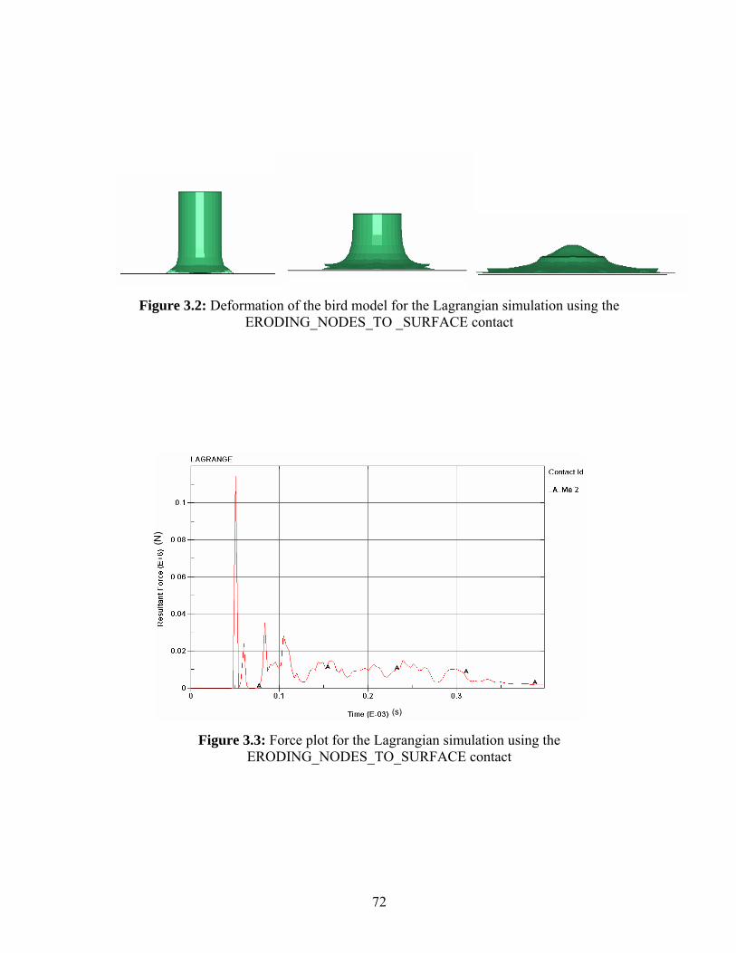
72
Figure 3.2: Deformation of the bird model for the Lagrangian simulation using the
ERODING_NODES_TO _SURFACE contact
Figure 3.3: Force plot for the Lagrangian simulation using the ERODING_NODES_TO_SURFACE contact
(s)
(N)
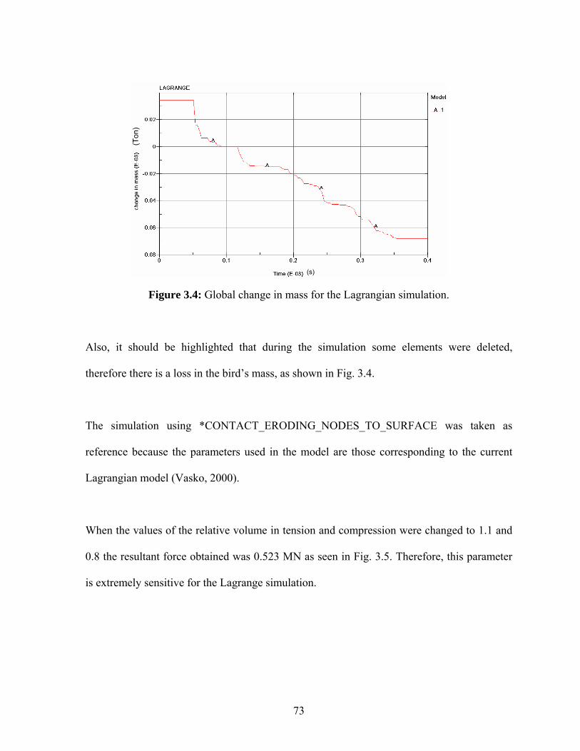
73
Figure 3.4: Global change in mass for the Lagrangian simulation.
Also, it should be highlighted that during the simulation some elements were deleted,
therefore there is a loss in the bird’s mass, as shown in Fig. 3.4.
The simulation using *CONTACT_ERODING_NODES_TO_SURFACE was taken as
reference because the parameters used in the model are those corresponding to the current
Lagrangian model (Vasko, 2000).
When the values of the relative volume in tension and compression were changed to 1.1 and
0.8 the resultant force obtained was 0.523 MN as seen in Fig. 3.5. Therefore, this parameter
is extremely sensitive for the Lagrange simulation.
(s)
(Ton
)

74
Figure 3.5: Resultant force in the interface for the Lagrange frontal impact on a rigid flat plate.
Forming Nodes to Surface Contact Type
Now we consider the *CONTACT_FORMING_NODES_TO_SURFACE to define
the contact between the bird model and the target. The deformation was not as smooth as it
was when using the *CONTACT_ERODING_NODES_TO_SURFACE. It can be seen in
Fig. 3.6 that at the final deformation, a considerable amount of the bird model actually
penetrates the target. The main reason is that this contact type is suitable for metal stamping
and not for rigid structures. Figure 3.7 presents the force plot generated by LS-DYNA for
this simulation.

75
Figure 3.6: Deformation of the bird model for the Lagrangian simulation using the FORMING_NODES_TO _SURFACE contact
Figure 3.7: Force plot for the Lagrangian simulation using the FORMING_NODES_TO_SURFACE contact
(s)
(N)

76
Figure 3.7 shows that the maximum force value obtained for this simulation was 0.0404 MN.
This value was 64.63% lower than the maximum value obtained in the previous Lagrangian
simulation. The fact that the deformation shows errors and that the behavior of the force was
very different when compared to force plots of previous simulations leads to the conclusion
that this simulation does not provide accurate results.
Nodes to Surface Contact Type
Lastly, we change the contact type to *CONTACT_NODES_TO _SURFACE. This is
a constraint based contact in which the forces are computed to keep the slave nodes in the
master surface. The deformation of this simulation presented instability error. This error was
similar to that observed in the simulation performed using *CONTACT_FORMING_
NODES_TO_SURFACE, as shown in Fig. 3.8. The force plot from this simulation (see Fig.
3.9) was exactly the same as the force plot from the previous simulation. This force plot is
the same as Fig. 3.7, resulting in a maximum force value was the same as in the previous
simulation, 0.0404 MN, 64.63% lower than the peak force in the simulation using the
*CONTACT_ERODING_ NODE_TO_SURFACE.
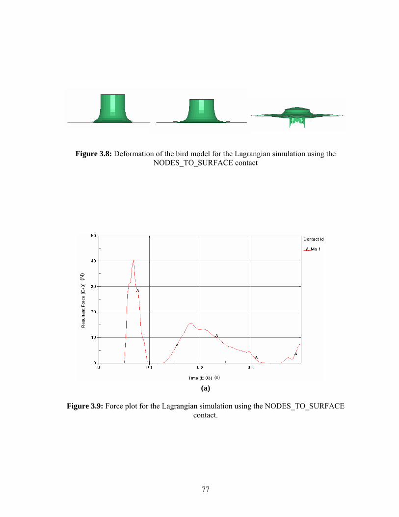
77
Figure 3.8: Deformation of the bird model for the Lagrangian simulation using the NODES_TO_SURFACE contact
(a)
Figure 3.9: Force plot for the Lagrangian simulation using the NODES_TO_SURFACE contact.
(s)
(N)

78
3.2.2 Using *MAT_ELASTIC_FLUID
For this simulation we changed the bird material from *MAT_NULL to
*MAT_ELASTIC_FLUID. Since the results produced using *MAT_NULL are not
acceptable due to the large margins of error, we decided to study to change the material
model for the bird. The same three types of contacts are studied for this material as well.
First, *CONTACT_ERODING_NODE_TO_SURFACE was used. A different outcome is
expected because the equation of state for this material is different and it is described in
section 2.1.2.
*CONTACT_ERODING_NODE_TO_SURFACE
Figure 3.10 shows how the bird deforms after the impact and the force plot is show in
Fig. 3.12. The maximum impact force obtained from this simulation was 0.0581 MN and it
was obtained at 44.9 µs. Since the pressure is needed in order to compare these results with
the test data provided by Barber et al. (1975), we calculated the impact area by measuring the
diameter of impact at the same time in which the peak force occurred. This area was only an
approximation to compute the maximum peak pressure. It was calculated measuring the
diameter of the impact area as shown in Figure 3.11. The diameter was 41.18 mm therefore
the approximated area was 1331.8 mm2. Thus the peak pressure is 43.66 MPa, which is has
9.15% difference when compared to that obtained by Barber et al. (1975).
Figure 3.10: Lagrangian bird deformation when using *MAT_ELASTIC_FLUID

79
Figure 3.11: Diameter in the peak force impact time.
Figure 3.12: Force plot for the Lagrangian case using elastic fluid material.

80
*CONTACT_FORMING_NODE_TO_SURFACE
Using the material elastic fluid the contact was changed to a forming contact type. The peak
force obtained in this simulation was 0.0403 MN and the diameter of the impact area was
43.9 mm. Using this values the peak pressure was calculated to be 26.67 MPa. Figure 3.13
shows the deformation of the bird for this simulation. Again we can see that the final
deformation penetrates the rigid plate and thus it is not recommended.
Figure 3.13: Force plot for the Lagrangian case using elastic fluid material.
*CONTACT_ NODE_TO_SURFACE
The last contact used was the contact node to surface. The curve for the force obtained for
this case was the similar to the one using forming contact type. The maximum force was
0.0403 MN and the impact diameter was the same as in the previous case. The deformation
was different as observed in Fig. 3.14. A comparison of the force obtained in the last three
simulations is show in Fig. 3.16

81
Figure 3.14: Force plot for the Lagrangian case using elastic fluid material.
3.2.3 Comparison of the Lagrangian Simulations
Three Lagrangian simulations were performed varying contact cards and bird material
types. The contact cards used were: *CONTACT_ERODING_NODES_TO_ SURFACE,
*CONTACT_FORMING_NODES_TO_SURFACE and *CONTACT_ NODES_TO_
SURFACE. The materials used were *MAT_NULL and *MAT_ELASTIC_ FLUID. There
is no difference between the results of the simulations using the *CONTACT_
FORMING_NODES_TO_SURFACE and *CONTACT_NODES_TO _SURFACE cards.
Figures 3.6 and 3.8 show that simulations with these contacts do not provide a smooth
deformation of the bird. Since a significant amount of the bird actually penetrates through the
target causes errors in the force and thus pressure values. As a consequence, the peak force
values obtained for these simulations were 64.63% lower than the values obtained in the
Lagrangian simulations using an eroding contact type.
On the other hand, the Lagrangian simulation performed using the *CONTACT
_ERODING_NODES_TO_SURFACE contact card provided the best deformation and the
force plots. Thus eroding contact type is the contact type recommended for the Lagrangian
bird model for bird-strike events against fan blades. In addition, the results for this simulation

82
are reliable and, thus, recommended as a standard. Figure 3.15 shows the results of the
Lagrangian simulations using *MAT_NULL superimposed on one plot.
Figure 3.15: Comparison of the Lagrangian simulations using *MAT_NULL
The peak pressure obtained using the eroding contact with MATERIAL_NULL was 117%
when compared with the test data. When using MATERIAL_ELASTIC_FLUID the
approximate pressure was 9.15% higher to that value obtained by Barber et al. (1975). Thus,
the bird with this material type is recommended and thus used as a reference to compare the
pressure values obtained with both SPH and ALE approaches. Table 3.3 shows the
comparison of the peak pressure for the different Lagrangian simulations. As observed when
using the material elastic fluid a higher convergence is was found with the test data.
Therefore, this simulation is used as a reference for comparison with ALE and SPH methods.
All the pressures were calculated using the approximate impact area calculated using the
diameter at the impact time.
(s)
0
2000040000
6000080000
100000120000
140000
4.00E-05 9.00E-05 1.40E-04 1.90E-04 2.40E-04 2.90E-04
Time (hours)
Forc
e (N
)
Lagrangian (ERODING_NODES_TO_SURFACELagrangian (FORMING_NODES_TO_SURFACE)Lagrangian (NODES_TO_SURFACE)
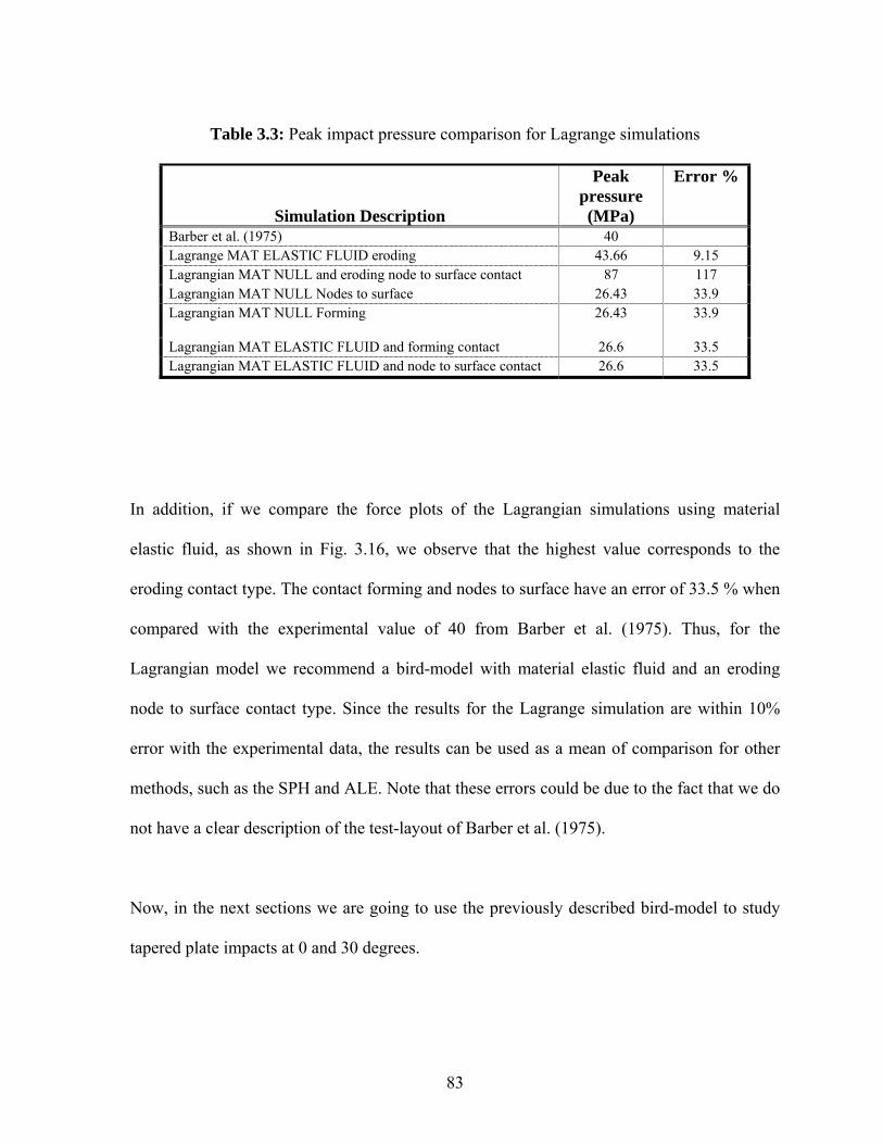
83
Table 3.3: Peak impact pressure comparison for Lagrange simulations
Simulation Description
Peak pressure (MPa)
Error %
Barber et al. (1975) 40 Lagrange MAT ELASTIC FLUID eroding 43.66 9.15 Lagrangian MAT NULL and eroding node to surface contact 87 117 Lagrangian MAT NULL Nodes to surface 26.43 33.9 Lagrangian MAT NULL Forming 26.43 33.9
Lagrangian MAT ELASTIC FLUID and forming contact 26.6 33.5 Lagrangian MAT ELASTIC FLUID and node to surface contact 26.6 33.5
In addition, if we compare the force plots of the Lagrangian simulations using material
elastic fluid, as shown in Fig. 3.16, we observe that the highest value corresponds to the
eroding contact type. The contact forming and nodes to surface have an error of 33.5 % when
compared with the experimental value of 40 from Barber et al. (1975). Thus, for the
Lagrangian model we recommend a bird-model with material elastic fluid and an eroding
node to surface contact type. Since the results for the Lagrange simulation are within 10%
error with the experimental data, the results can be used as a mean of comparison for other
methods, such as the SPH and ALE. Note that these errors could be due to the fact that we do
not have a clear description of the test-layout of Barber et al. (1975).
Now, in the next sections we are going to use the previously described bird-model to study
tapered plate impacts at 0 and 30 degrees.
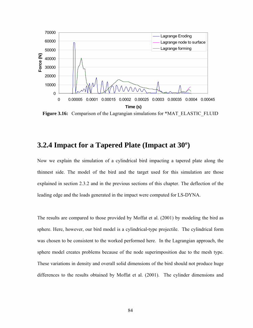
84
0
10000
20000
30000
40000
50000
60000
70000
0 0.00005 0.0001 0.00015 0.0002 0.00025 0.0003 0.00035 0.0004 0.00045
Time (s)
Forc
e (N
)Lagrange ErodingLagrange node to surfaceLagrange forming
Figure 3.16: Comparison of the Lagrangian simulations for *MAT_ELASTIC_FLUID
3.2.4 Impact for a Tapered Plate (Impact at 30º)
Now we explain the simulation of a cylindrical bird impacting a tapered plate along the
thinnest side. The model of the bird and the target used for this simulation are those
explained in section 2.3.2 and in the previous sections of this chapter. The deflection of the
leading edge and the loads generated in the impact were computed for LS-DYNA.
The results are compared to those provided by Moffat et al. (2001) by modeling the bird as
sphere. Here, however, our bird model is a cylindrical-type projectile. The cylindrical form
was chosen to be consistent to the worked performed here. In the Lagrangian approach, the
sphere model creates problems because of the node superimposition due to the mesh type.
These variations in density and overall solid dimensions of the bird should not produce huge
differences to the results obtained by Moffat et al. (2001). The cylinder dimensions and

85
properties are same as those used in the flat plate impact (Table 2.4) with the difference that
the impact velocity is 477.4 m/s (1067 mph).
The boundary nodes of the plate corresponding to both sides were fixed with *SPC_
BOUNDARY card. The tapered section of the plate was simulated by increasing the mesh
and assigning different parts with different *SECTION_SHELL cards. The cards differ from
each other in the thickness of the elemental nodes. Five different parts were created for the
tapered section of the plate. The thickness of these different parts is shown in Table 3.3.
Parts are illustrated with different colors in the plate shell in Fig. 3.17.
Table 3.4: Thickness for each part for the tapered plate.
Part Thickness for the four different
nodes of the shell element (mm) 6 1.6 7 1.382 8 1.164 9 0.946 10 0.728 11 0.51
Moffat et al. (2001) found that the maximum deflection in the leading edge was 1.05 in when
a bird impacts the simulated tapered plate at 30 degrees. The impact angle of the bird was 30
degrees and was measured between the axis of the cylinder and the plane of the tapered plate
as showed in Fig. 3.17. The mesh of the cylinder was the same as previously described.
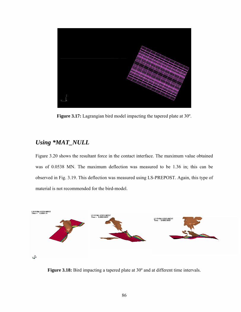
86
Figure 3.17: Lagrangian bird model impacting the tapered plate at 30º.
Using *MAT_NULL
Figure 3.20 shows the resultant force in the contact interface. The maximum value obtained
was of 0.0538 MN. The maximum deflection was measured to be 1.36 in; this can be
observed in Fig. 3.19. This deflection was measured using LS-PREPOST. Again, this type of
material is not recommended for the bird-model.
Figure 3.18: Bird impacting a tapered plate at 30º and at different time intervals.
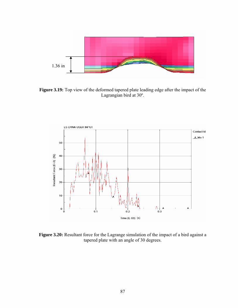
87
Figure 3.19: Top view of the deformed tapered plate leading edge after the impact of the Lagrangian bird at 30º.
Figure 3.20: Resultant force for the Lagrange simulation of the impact of a bird against a tapered plate with an angle of 30 degrees.
(s)
(N)
1.36 in

88
Using *MAT_ELASTIC_FLUID
Figure 3.21 shows the deformation of the tapered plate during the impact when the bird is
modeled using *MAT_ELASTIC_FLUID. As observed some elements are eliminated
during calculations due to negative volumetric strains failure. Figure 3.22 shows the top
view of the tapered plate leading edge deflection.
The maximum deflection was found to be 1.19 in as seen in Fig 3.22. This deflection was
measured using the tool of the LS-PREPOST to measure the change in coordinates using as
point of reference the position of the corner of the plate which is constrained in translation
and rotation in the x, y and z directions. In addition, Fig. 3.23 shows the resultant force in the
contact interface and the maximum value was 0.056 MN.
Figure 3.21: Bird impacting a tapered plate at 30º and at different time intervals.

89
Figure 3.22: Top view of the deformed tapered plate leading edge after the impact of the Lagrangian bird at 30º.
Figure 3.23: Resultant force for the Lagrange simulation of the impact of a bird against a
tapered plate with an angle of 30 degrees.
1.19 in

90
Table 3.5: Maximum normal deflection comparison.
Tapered impact simulation at 30 degrees
Maximum normal deflection (in)
Error %
Moffat et al. (2001) 1.05 ----- Lagrange using *MAT_NULL 1.36 29.8
Lagrange Using *MAT_ELASTIC_FLUID
1.19 13.3
The simulation using material elastic fluid and eroding node to surface gave us acceptable
results when comparing to the work done by Moffat. Only a 13.3 % of error, taking in
consideration that the shape of the bird used in our case was different from that used by
Moffat. Thus, the force generated in this case can be used as reference to compare the results
using both SPH and ALE methods. One reason why the better approximation is the Lagrange
simulation using the material elastic fluid could be because the material elastic fluid
computes the stresses that cause the deformation in the bird or the deviatoric stresses. Also,
the material null does not take account for this stresses the energy in the impact will be
absorbed by the target resulting in a higher force produced.
3.2.5 Impact Simulation for a Tapered Plate (at 0º)
In this simulation the angle of impact was varied to 0 degrees. The bird and plate properties
were the same as the used in the 30 degrees impact. Figure 3.24 shows the geometrical model
for this case.

91
Figure 3.24: Model of the tapered plate for the Lagrangian impact simulation.
USING *MAT_NULL
Figure 3.25 shows the deformation of the bird impacting the tapered plate at different times.
The deformation pattern of the tapered plate obtained during this simulation was small
because the bird was sliced in two parts (Moffat et al., 2001). During simulations, some
elements of the bird were deleted which were produced due to failing in the negative tensile
or compressive volumetric strains. Figure 3.26 shows the tapered plate leading edge
deformation seen from top.
Figure 3.25: Deformation of the tapered plate at different time intervals for the Lagrange
description.

92
Figure 3.26: Top view of the tapered plate deflection at the leading edge for the Lagrange simulation at 0º.
The maximum resultant force on the impacting surface is approximately 0.0142 MN as
shown in Fig. 3.27. This graph is not as smooth as that obtained in the flat-plate impact
simulation. The interaction that produced the eroding contact type caused several decays and
increases of the pressure.
02000
4000
6000
8000
10000
1200014000
16000
0.00E+00 1.00E-04 2.00E-04 3.00E-04 4.00E-04 5.00E-04
Time (s)
Forc
e (N
)
Lagrange Null
Figure 3.27: Plot of the resultant force for the Lagrange simulation of the impact of a bird at 0 degrees against a tapered plate.
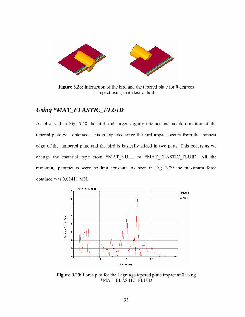
93
Figure 3.28: Interaction of the bird and the tapered plate for 0 degrees impact using mat elastic fluid.
Using *MAT_ELASTIC_FLUID
As observed in Fig. 3.28 the bird and target slightly interact and no deformation of the
tapered plate was obtained. This is expected since the bird impact occurs from the thinnest
edge of the tampered plate and the bird is basically sliced in two parts. This occurs as we
change the material type from *MAT_NULL to *MAT_ELASTIC_FLUID. All the
remaining parameters were holding constant. As seen in Fig. 3.29 the maximum force
obtained was 0.01411 MN.
Figure 3.29: Force plot for the Lagrange tapered plate impact at 0 using *MAT_ELASTIC_FLUID
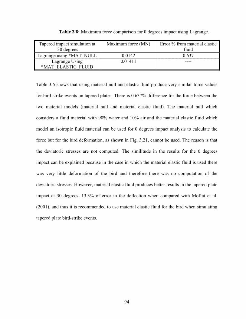
94
Table 3.6: Maximum force comparison for 0 degrees impact using Lagrange.
Tapered impact simulation at 30 degrees
Maximum force (MN) Error % from material elastic fluid
Lagrange using *MAT_NULL 0.0142 0.637 Lagrange Using
*MAT_ELASTIC_FLUID 0.01411 ----
Table 3.6 shows that using material null and elastic fluid produce very similar force values
for bird-strike events on tapered plates. There is 0.637% difference for the force between the
two material models (material null and material elastic fluid). The material null which
considers a fluid material with 90% water and 10% air and the material elastic fluid which
model an isotropic fluid material can be used for 0 degrees impact analysis to calculate the
force but for the bird deformation, as shown in Fig. 3.21, cannot be used. The reason is that
the deviatoric stresses are not computed. The similitude in the results for the 0 degrees
impact can be explained because in the case in which the material elastic fluid is used there
was very little deformation of the bird and therefore there was no computation of the
deviatoric stresses. However, material elastic fluid produces better results in the tapered plate
impact at 30 degrees, 13.3% of error in the deflection when compared with Moffat et al.
(2001), and thus it is recommended to use material elastic fluid for the bird when simulating
tapered plate bird-strike events.
95
Chapter 4. Bird-Strike Modeling Based on SPH Formulation
The Lagrangian method is the most commonly used when designing fan blades. This
Lagrangian description has been used to create models for both the bird and fan blades.
However, this description causes losses of the bird mass due to the fluid behavior of the bird,
which causes large distortions in the bird model. This mass loss may reduce the real loads
applied to the fan blade, which is the reason why the Smoothed Particle Hydrodynamics
(SPH) is being studied in this work. LS-DYNA, an impact-dynamic finite element software,
has integrated the SPH formulation to model this fluid-structure interaction problem. In this
work, the SPH method is going to be evaluated and further developed into a standard
approach to modeling bird-strike events.
In the Lagrangian model, the numerical mesh moves and distorts with the physical material,
allowing to accurately and efficiently tracking material interfaces and the incorporate
complex material models. One disadvantage of this method is the negative volume error
which occurs as a result of mesh tangling do to its sensitivity to distortion, resulting in small
time steps and sometimes loss of accuracy.
The SPH is a mesh-less or griddles technique that does not suffer from the normal problems
of grid tangling in large deformation problems. The major advantages of the SPH technique
is that it does not require a numerical grid and, since it is a Lagrangian method by nature, it

96
allows efficient tracking of material deformations and history-dependent behavior. Because
the SPH method has not been fully developed there remain some issues in the areas of
stability, consistency, and conservation. Lagrangian motions of mass points or particles are
really interpolation points, which are approximated by a cubic B-spline function. Unlike
finite element representations for a structure, this finite element model does not exhibit a
fixed connectivity between adjacent elements during the impact event. The determination of
which elements are nearest neighbors is limited by the search radius. The search radius
defines the maximum distance from the center node that an element may search for nearest
neighbors and becomes in effect a measure of the fluid cohesive strength.
4.1 SPH Model for the Bird-Strike Event
4.1.1 Pre-processing variables for the SPH model
The dimensions and overall properties for the bird and the targets used here are
provided in section 2.3.2. The target used in all the SPH simulation has a Lagrangian
description, therefore the model of the flat rigid plate and the tapered plate are those used in
the Lagrangian simulations, presented in chapter 3. The explanation of the construction of the
SPH bird model is discussed in section 4.2.1. Table 4.1 summarizes the general parameters
used for the SPH bird model.
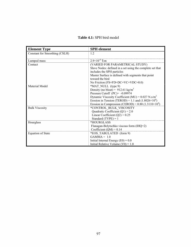
97
Table 4.1: SPH bird model
Element Type SPH element Constant for Smoothing (CSLH) 1.2
Lumped mass 2.9×10⁻⁸ Ton Contact (VARIED FOR PARAMETRICAL STUDY)
Slave Nodes: defined in a set using the complete set that includes the SPH particles Master Surface is defined with segments that point toward the bird No Friction (FS=FD=DC=VC=VDC=0.0)
Material Model *MAT_NULL (type 9) Density (no bloat) = 912.61 kg/m3 Pressure Cutoff (PC)= -0.09974 Dynamic Viscosity Coefficient (MU) = 0.027 N.s/m2 Erosion in Tension (TEROD) = 1.1 and (1.8026×10⁴) Erosion in Compression (CEROD) = 0.80 (1.3110×10⁴)
Bulk Viscosity *CONTROL_BULK_VISCOSITY Quadratic Coefficient (Q1) = 2.0 Linear Coefficient (Q2) = 0.25 Standard (TYPE) = 1
Hourglass *HOURGLASS Flanagan-Belytschko viscous form (IHQ=2) Coefficient (QM) = 0.14
Equation of State *EOS_TABULATED (form 9) GAMMA = 1.0 Initial Internal Energy (E0) = 0.0 Initial Relative Volume (V0) = 1.0

98
4.2 Bird-Strike Simulation
As in the Chapter 3, two different simulations were performed. The first simulation
consisted in the bird strike event against solid rigid plates as done by Barber et al. (1975).
The second simulation model was based in the work of Moffat et al. (2001), bird-strikes on
tapered plates. All simulations using the SPH model are compared with their respective
available test data and the Lagrangian models.
In the next sections we explain the SPH model and the results obtained by the simulations
using LS-DYNA preprocessor and ETA-FEMB post processor. The bird will follow the
parameters of the Lagrange Bird previously discussed and the target plate model is identical
to the plate used in the Barber et al. (1975).
4.2.1 SPH element generation
In order to achieve a fair comparison with the Lagrange simulations, we kept the
same bird properties as in the Lagrangian case. Because the SPH model is represented by a
group of elements or small spheres, and is not continuous along the whole space they are
occupying, it is necessary to calculate the physical properties for each element by taking into
account that each element should have the same bird density. It is also important to highlight
that the sum of masses of all small elements or spheres must be equal to the mass of the bird.

99
The rigid and tapered plates used for the SPH model have the same dimensions and
properties as in the case of the Lagrangian simulation. To model the bird, first a square mesh
with equivalent sides to the pre-calculated diameter are constructed, and then extruded to a
length with different number of subdivisions, as seen in Fig. 4.1(a). The elements located in
the square mesh are eliminated to approximate the mesh shape to that of the circular
(cylindrical) mesh used in the Lagrangian simulation, as shown in Figs. 4.1(b) and 4.1(c).
The remaining nodes are used to calculate the mass and dimensions of each spherical
element, and the SPH particles were constructed in each remaining node (Goyal et al.,
2006a).
(a)
(b) (c)
Figure 4.1: SPH element generation for the bird model

100
The following equation shows how the lumped mass for each SPH element is calculated:
nodesmmassLumped total
#= (4.1)
Note that the number of nodes is equal to the number SPH elements. For the shot reproduced
the dimensions of the bird (cylindrical representation) were:
mmD 4431.41=
mmL 60=
36.912ρ
m
kg=
32
7.809364
π mmLDV =⋅⋅
=
kgVm 073863.0ρ =⋅=
Three simulations where performed: rigid flat plate with frontal impact, and deformable
tapered plate with 0 and 30 degree impact.
4.3 Bird-Strike Against Rigid Flat Plate
4.3.1 Parameter Variation for SPH Modeling
Several simulations are performed in which the variables inside the *CONTROL_
SPH card, type of contact and number of SPH particles were changed in order to study their
sensitivity on the impact loads and pressures. For all the contacts, the flat plate was assigned
as the master part and the SPH bird as the slave part.

101
Here, we explain the variables that affect directly the output data for a bird-strike event
modeled in LS-DYNA using the SPH approach. The two most important parameters that
influenced the desired response are the type of contact between the SPH particles and the
target surface, and the Particle Approximation Theory (keyword: FORM inside the SPH card
*CONTROL_SPH). The contacts used for the simulations performed included only those
that define contact between the SPH nodes to the surface of the Lagrangian target these types
of contacts are one-way contact types.
It is important to note that the activation of the control card *CONTROL_ HOURGLASS
and assigning the parameters of energy in the *HOURGLASS card do not affected the output
results. The obtained results are compared with the Lagrange simulations of a cylinder
impacting a circular rigid flat plate.
The FORM parameter (Particle Approximation Theory parameter) inside the *CONTROL_
SPH card can be changed and set to FORM=1 (remoralization approximation). This
generates a deformation similar to that predicted by Wilbeck and Barber (1978) of the
impacting cylinder reducing the effect of bouncing of the particles when entering in contact
with the target. The parameter has a default value of FORM=0. By changing this parameter,
a bounce-off effect is produced and thus it affects the interaction of the upcoming particles
when entering in contact with the target and the particles already in contact with it.

102
Figure 4.2: Side view of the simulation for
*CONTACT_AUTOMATIC_NODE_TO_SURFACE and FORM=0.
Figure 4.3: Simulation results for the SPH with FORM=0 and *CONTACT_AUTOMATIC_NODE_TO_SURFACE.

103
Figures 4.2 and 4.3 illustrates the interaction for FORM=0 and *CONTACT_ AUTOMATIC
_NODE_TO_SURFACE_ID. Figures 4.4 and 4.5 shows the results for the simulation when
the FORM=1. The maximum force obtained for this simulation was 0.048 MN which differs
from the 0.0581 MN of the Lagrange simulation with a 17.38% of error.
The variable NCBS (Number of Cycles Between particle Sorting) of the *CONTROL_SPH
card is varied between 2 and 5. The same force at the interface surface is used for each value
for the NCBS variable. Figure 4.6 shows the deformation at different time intervals for the
case when NCBS is equal to 2. The final deformation is in good agreement to that predicted
by Wilbeck and Barber (1978). Figures 4.8 and 4.9 show the results for the SPH simulation
by setting NCBS=5. By comparing Figs. 4.7 and 4.9, it is observed that there is no difference
in the resultant force at the interface of the SPH bird and the Shell Target. Both simulations
gave a peak force of 5.4 kN. Thus, NCBS is a nonaffecting variable in the simulation. The
contact used for this simulation was *CONTACT_CONSTRAINT_NODE_TO_SURFACE
contact type. The same simulation is included in the contact variation for 8700 SPH particles
in section 4.3.2.
Figure 4.4: Sequence at different time intervals of deformation of the SPH bird (FORM=1 and *CONTACT_AUTOMATIC_NODE_TO_SURFACE).

104
Figure 4.5: Resultant force for SPH simulation with FORM=1 and
*CONTACT_AUTOMATIC_NODE_TO_SURFACE.
Figure 4.6: Deformation of the SPH bird for different time intervals (NCBS= 2)
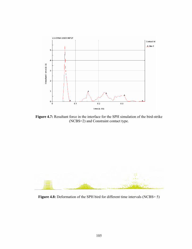
105
Figure 4.7: Resultant force in the interface for the SPH simulation of the bird-strike (NCBS=2) and Constraint contact type.
Figure 4.8: Deformation of the SPH bird for different time intervals (NCBS= 5)

106
Figure 4.9: Resultant force in the interface for the SPH simulation of the bird-strike (NCBS=5)
4.3.2 Contact Variation for 8700 SPH particles
Now, we study the effect of various contact types for the bird model composed of 8700 SPH
particles. The goal is to determine the best contact type for bird-strike modeling. The final
results are compared to those obtained using the Lagrangian simulation discussed in section
3.2.1, in which the eroding contact type was used in conjunction with the material elastic
fluid.
For this simulation a new mesh pattern is created for the bird. Two different mesh
densities are used. As observed in Fig. 4.10, the higher meshing resolution is placed at the
center of the bird to allow impact of a larger amount of SPH particles with the simulated
transducer.

107
Figure 4.10: Top view of the created SPH particles and the original solid mesh.
Figure 4.11: Side view of the cylinder impacting the plate at different time intervals
(*CONCTACT_ERODING_NODE_TO_SURFACE)

108
Eroding Node to Surface Contact Type
The contact type for this simulation was changed to *ERODING_NODE_TO_
SURFACE and FORM=1. As seen in Fig. 4.11, for this contact type, there exist a bounce-off
effect higher than when using the *CONTACT_CONSTRAINT_NODE_TO_SURFACE and
FORM=1 but lower than when using the *AUTOMATIC_NODE_TO_SURFACE and
FORM=0. Figure 4.12 shows that the maximum force obtained in this case was of 0.489 MN
approximately, which has an error of 741% when compared with the 0.0581 MN peak force
obtained using the standard Lagrangian case for the same contact type. The reason for this
difference is the difference in the material and the equation of state used in both simulations.
Figure 4.13 shows that for this simulation there was no loss in the overall mass of the system.
Figure 4.12: Resultant force for SPH simulation with *CONCTACT_ERODING_NODE_TO_SURFACE and FORM=1.
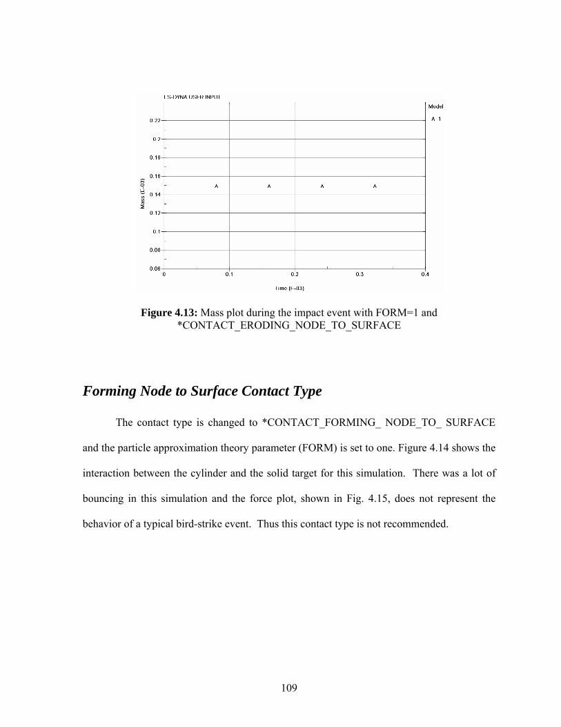
109
Figure 4.13: Mass plot during the impact event with FORM=1 and *CONTACT_ERODING_NODE_TO_SURFACE
Forming Node to Surface Contact Type
The contact type is changed to *CONTACT_FORMING_ NODE_TO_ SURFACE
and the particle approximation theory parameter (FORM) is set to one. Figure 4.14 shows the
interaction between the cylinder and the solid target for this simulation. There was a lot of
bouncing in this simulation and the force plot, shown in Fig. 4.15, does not represent the
behavior of a typical bird-strike event. Thus this contact type is not recommended.
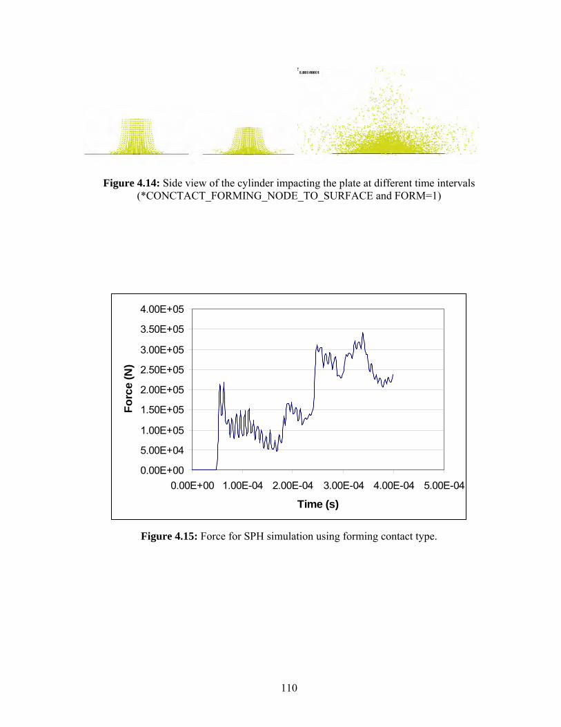
110
Figure 4.14: Side view of the cylinder impacting the plate at different time intervals (*CONCTACT_FORMING_NODE_TO_SURFACE and FORM=1)
0.00E+00
5.00E+04
1.00E+05
1.50E+05
2.00E+05
2.50E+05
3.00E+05
3.50E+05
4.00E+05
0.00E+00 1.00E-04 2.00E-04 3.00E-04 4.00E-04 5.00E-04
Time (s)
Forc
e (N
)
Figure 4.15: Force for SPH simulation using forming contact type.

111
Figure 4.16: SPH progression of the bird deformation for a rigid wall contact.
Bird-Strike Event Using a Rigid Wall Contact
Now we changed the contact from the *CONTACT_CONSTRAINT_NODE_TO_
SURFACE to *RIGID_WALL_PLANAR _FORCE. This last card is used to define a rigid
wall. Also, a segment was created for the shell elements of the target. It was necessary to
define a *DATABASE_RWFORC card for the creation of the database for the forces
generated in the segment set. The *BOUNDARY_SPC card was eliminated. Figure 4.16
shows the deformation of the SPH bird for this simulation. The deformation behavior may be
acceptable because not much bouncing effect is observed.
The resultant force is presented in Fig. 4.17. This data was extracted from the rwforc file
created by LS-DYNA. The behavior was similar to the previous simulations. It was observed
that there exists a short time interval after the peak force where the calculated force vanishes
afterwards. Table 4.2 provides the force values compared with this and the Lagrangian
simulation.

112
Figure 4.17: Resultant normal force using the rigid wall contact.
Table 4.2: Comparison between SPH and Lagrangian simulations using a rigid wall
Simulation Description Peak Force
(MN) Error %
Rigid Wall 0.34 261.53 Lagrangian Elastic Fluid 0.0581 ----

113
It is observed that the peak value of the force for the SPH simulation using a rigid wall
constraint on the target were 261.53% higher than the result obtained by the Lagrangian
simulation. The behavior after the impact for the SPH Rigid Wall simulation was similar to
the behavior of the Lagrangian simulation, although it had less peaks (the plot was smoother)
and did not decrease to zero except after the initial impact. However, the peak value of the
force using the rigid wall constraint was significantly different to the peak value from the
Lagrangian simulation than the value obtained using two targets. Thus, this contact is not
recommended for bird-strike events.
Using Two Targets and Rigid Wall contact
Now, we use the same SPH bird-model as in previous simulations but with two plates
as the targets and a rigid wall contact type. The SPH model is built using 8,700 SPH particles
and arranged in a cylindrical geometry. Two plates were used to allow movement to one of
the plates. The top plate was not constrained to any degree of freedom, but the bottom plate
was constrained using the *BOUNDARY_SPC card. The distance between the plates was 1
mm, allowing small displacement of the upper plate before any contact with the bottom plate.
The purpose was to observe the change in forces and pressures generated between the SPH
particles and the top plate. It was necessary to define two contacts, one between the bird and
the upper target and other between the first target and the bottom and constraint target. If
there is no definition of these contacts no force will be calculated in the interface. Figure 4.18
presents the interaction between the bird and the plates.

114
Figure 4.18: Deformation of the SPH Bird and the plates.
a) Bottom plate
b) Top plate
Figure 4.19: Resultant force in the interface of the bird and the targets. a) Bottom plate, b) Top plate

115
The *DATABASE_NCFORC card was also defined. This card stores the nodal interface
forces and allows pressure plot for this interface. In order to create this database, the SPR and
MPR variables from the contact card are changed to one. The force plot for selected nodes is
shown in Fig. 4.19. The results show similar pattern from previous simulations: the force
decreases to almost zero after the initial impact.
Figure 4.19 shows the resultant force values at the interface between the bird and the targets.
It is observed that in both contact interfaces the behavior was similar although the peak value
of the force varied. The peak force values were approximately 0.325 MN and 0.78 MN. The
first value (0.325 MN) had an error of 459% if compared with the Lagrange simulation in
which the peak force was 0.0581 MN when using TEROD=1.1. On the other hand, the value
of 0.78 MN had an error of 1242% which was higher than the values obtained in other
simulations and is the force generated in the top plate (which was not constrained). This force
was higher because the plate was impacted by the bird-model and then impacted the bottom
plate.
The force values were compared between this simulation and the Lagrangian simulation and
the results are shown in Table 4.3. The huge differences between this method and the
Lagrange make this approach an unacceptable one.

116
Table 4.3: Comparison of results between the SPH simulation with two targets and the Lagrangian simulation
Simulation DescriptionPeak Force
(MN) Error %
0.325 459 Two Targets (SPH)
0.78 1242 Lagrangian MAT ELASTIC FLUID 0.0581
*Mat_Rigid Material Model for a Simulated Solid Transducer
Now we use a solid transducer in the center of the target to measure the pressure in
that region. The material of this solid transducer was varied from *MAT_PIECE_WISE_
LINEAR_PLASTICITY to *MAT_RIGID. The contact used was *CONTACT_
CONSTRAINED_NODE_TO_SURFACE.
The deformation of the bird is shown in Fig. 4.20. The behavior of the deformation of the
bird resembles the one predicted by Barber et al. (1975). In addition, there was not much
bouncing of the particles after the impact. However, the resultant force in the interface of the
bird and the solid transducer was almost 100% lower when compared to the Lagrangian case,
as seen in Fig. 4.21. All the force values for previous simulations were of the order 106 N
and the results for this simulation were in the order of 103 N. This simulation did not provide
acceptable results and thus is not recommended.

117
Figure 4.20: Deformation of the SPH bird for *MAT_RIGID.
Figure 4.21: Resultant force in the interface of the bird and the target for *MAT_RIGID.
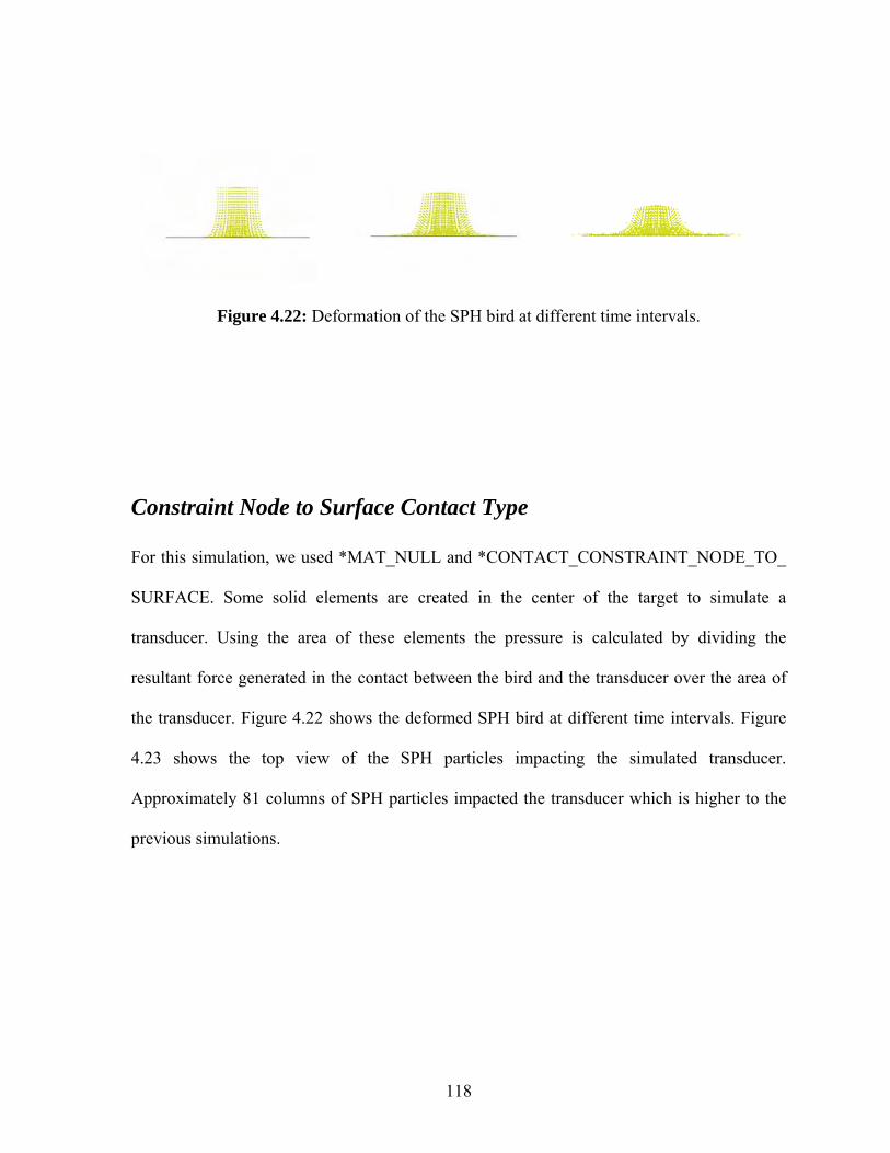
118
Figure 4.22: Deformation of the SPH bird at different time intervals.
Constraint Node to Surface Contact Type
For this simulation, we used *MAT_NULL and *CONTACT_CONSTRAINT_NODE_TO_
SURFACE. Some solid elements are created in the center of the target to simulate a
transducer. Using the area of these elements the pressure is calculated by dividing the
resultant force generated in the contact between the bird and the transducer over the area of
the transducer. Figure 4.22 shows the deformed SPH bird at different time intervals. Figure
4.23 shows the top view of the SPH particles impacting the simulated transducer.
Approximately 81 columns of SPH particles impacted the transducer which is higher to the
previous simulations.

119
Figure 4.23: Top view of the impact of the SPH particles against the transducer.
Figure 4.24: Resultant force in the interface for the SPH simulation.

120
Fig. 4.24 shows the resultant force at the interface when the SPH bird impacts the transducer.
The area of the transducer was 12x12 mm (144 mm2). The pressure is given in Fig. 4.25. The
peak force obtained in this case was 0.0054 MN. Then, dividing this value over 144 mm2 the
pressure for this simulation was 37.23 MPa (5409.7 psi) which was 7.05% lower than the 40
MPa (5801.2 psi) measured by Barber et al. for shot 5126A. However the steady state phase
of the simulation, as observed in the experimental test, is not captured. Note that this
simulation was the same used in the previous section to study the influence of the NCBS
parameter in the results
0.0
5.0
10.0
15.0
20.0
25.0
30.0
35.0
40.0
0.00E+00 1.00E-04 2.00E-04 3.00E-04 4.00E-04 5.00E-04
Time (s)
Pres
sure
(Mpa
)
SPH 8700 ConstraintTransducer
Figure 4.25: Pressure in the interface for the SPH simulation.
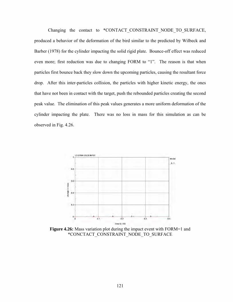
121
Changing the contact to *CONTACT_CONSTRAINT_NODE_TO_SURFACE,
produced a behavior of the deformation of the bird similar to the predicted by Wilbeck and
Barber (1978) for the cylinder impacting the solid rigid plate. Bounce-off effect was reduced
even more; first reduction was due to changing FORM to “1”. The reason is that when
particles first bounce back they slow down the upcoming particles, causing the resultant force
drop. After this inter-particles collision, the particles with higher kinetic energy, the ones
that have not been in contact with the target, push the rebounded particles creating the second
peak value. The elimination of this peak values generates a more uniform deformation of the
cylinder impacting the plate. There was no loss in mass for this simulation as can be
observed in Fig. 4.26.
Figure 4.26: Mass variation plot during the impact event with FORM=1 and
*CONCTACT_CONSTRAINT_NODE_TO_SURFACE

122
0.05.0
10.015.020.025.030.035.040.045.050.0
0.00E+00 1.00E-04 2.00E-04 3.00E-04 4.00E-04Time (s)
Pres
sure
(MPa
)
Lagrange Elastic Fluid
SPH Constraint 8700partilces
Figure 4.27: Comparison of pressure plots for Lagrangian and SPH simulation using constraint contact type for 8700 particles.
Comparing SPH (8,700 Particles) and Lagrangian Simulations
Figure 4.27 shows the SPH simulation that best converged to the Lagrangian solution
in term of the pressure generated was when using a *CONTACT_CONSTRAINT_
NODE_TO_SURFACE contact type. As explained before, a simulated transducer was used
to compute the pressure. The percentage of error in this method was 6.75% if compared with
the test data and 14.4% if compared with the Lagrangian case. The pressure comparison for
different SPH simulation with test data and the Lagrangian case is shown in Table 4.4.
Table 4.4: Pressure comparison between SPH and Lagrangian simulations
Simulation Description Material Contact Type
Number of Particles
Peak Pressure (MPa)
Error %
Barber et al. (1975) N/A N/A N/A 40 -----
Lagrange Elastic Fluid Eroding N/A 43.6 9.15
SPH Null Eroding 8,700 376 840 Rigid Wall Null Rigid wall 8,700 261 552
250 525 Two Targets (SPH) Null Rigid wall 8,700
600 1400 SPH with simulated
transducer Null Constraint 8,700 37.3 6.75
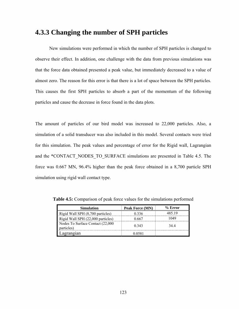
123
4.3.3 Changing the number of SPH particles New simulations were performed in which the number of SPH particles is changed to
observe their effect. In addition, one challenge with the data from previous simulations was
that the force data obtained presented a peak value, but immediately decreased to a value of
almost zero. The reason for this error is that there is a lot of space between the SPH particles.
This causes the first SPH particles to absorb a part of the momentum of the following
particles and cause the decrease in force found in the data plots.
The amount of particles of our bird model was increased to 22,000 particles. Also, a
simulation of a solid transducer was also included in this model. Several contacts were tried
for this simulation. The peak values and percentage of error for the Rigid wall, Lagrangian
and the *CONTACT_NODES_TO_SURFACE simulations are presented in Table 4.5. The
force was 0.667 MN, 96.4% higher than the peak force obtained in a 8,700 particle SPH
simulation using rigid wall contact type.
Table 4.5: Comparison of peak force values for the simulations performed
Simulation Peak Force (MN) % Error Rigid Wall SPH (8,700 particles) 0.336 485.19 Rigid Wall SPH (22,000 particles) 0.667 1049 Nodes To Surface Contact (22,000 particles) 0.343 34.4
Lagrangian 0.0581
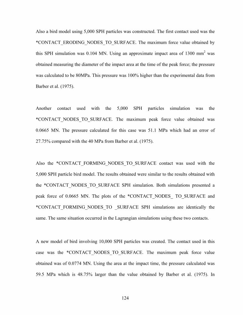
124
Also a bird model using 5,000 SPH particles was constructed. The first contact used was the
*CONTACT_ERODING_NODES_TO_SURFACE. The maximum force value obtained by
this SPH simulation was 0.104 MN. Using an approximate impact area of 1300 mm2 was
obtained measuring the diameter of the impact area at the time of the peak force; the pressure
was calculated to be 80MPa. This pressure was 100% higher than the experimental data from
Barber et al. (1975).
Another contact used with the 5,000 SPH particles simulation was the
*CONTACT_NODES_TO_SURFACE. The maximum peak force value obtained was
0.0665 MN. The pressure calculated for this case was 51.1 MPa which had an error of
27.75% compared with the 40 MPa from Barber et al. (1975).
Also the *CONTACT_FORMING_NODES_TO_SURFACE contact was used with the
5,000 SPH particle bird model. The results obtained were similar to the results obtained with
the *CONTACT_NODES_TO_SURFACE SPH simulation. Both simulations presented a
peak force of 0.0665 MN. The plots of the *CONTACT_NODES_ TO_SURFACE and
*CONTACT_FORMING_NODES_TO _SURFACE SPH simulations are identically the
same. The same situation occurred in the Lagrangian simulations using these two contacts.
A new model of bird involving 10,000 SPH particles was created. The contact used in this
case was the *CONTACT_NODES_TO_SURFACE. The maximum peak force value
obtained was of 0.0774 MN. Using the area at the impact time, the pressure calculated was
59.5 MPa which is 48.75% larger than the value obtained by Barber et al. (1975). In

125
comparison with the Lagrangian simulation the peak force obtained was 33.21% higher than
the peak force of the Lagrange simulation using a eroding contact type and material elastic
fluid. This force was 92% higher than the Lagrangian peak force using a node to surface
contact type and a material null.
Another SPH model was created with 2,178 particles. This model was created to evaluate the
trend that was found with the 5,000 and 10,000 SPH particle models (when the number of
particles increased, the force at the impact also increased). The 2,000 SPH particle model
was subjected to impact using the *CONTACT_NODES_TO_SURFACE contact card. The
trend that was mentioned before seems to be true, because the peak force value obtained for
the 2,000 SPH particle model was 0.0633 MN, 4.81% lower than the values obtained for the
5,000 SPH particle models and 18.21% lower than the results for the 10,000 SPH particle
model.
Table 4.6: Pressure comparison for particle variation in the SPH simulations.
Contact
Material
Type Number
of Particles
Peak Pressure
Value (MPa)
% Error From Test Data
Barber et al. (1975) N/A N/A N/A 40 ---- *CONTACT_ERODING_NODES_TO_SURFACE Elastic Fluid Lagrangian N/A 43.6 9.15
*CONTACT_ERODING_NODES_TO_SURFACE Null Lagrangian N/A 87.6 119
*CONTACT_ERODING_NODES_TO_SURFACE Null SPH 5,000 80 100
*CONTACT_NODES_TO_SURFACE Null Lagrangian N/A 31.07 22.32
*CONTACT_NODES_TO_SURFACE Null SPH 2,000 48.7 21.75 *CONTACT_NODES_TO_SURFACE Null SPH 5,000 51.1 27.75
*CONTACT_NODES_TO_SURFACE Null SPH 10,000 59.5 48.75

126
From Table 4.6, it can be stated that for a constant contact for the simulations performed
when the number of SPH particles was increased, the maximum pressure value obtained from
the simulation also increased. All the pressures were calculated using the approximate area
measured at the time in which the peak force occurs for each simulation. As observed there
was no convergence of the pressure for any of the cases showed in Table 4.6.
Figure 4.28: SPH simulations of shot 5126 A for different number of particles.
Pre-processing
Results
(22,000 SPH particles) (5,000 SPH particles) (10,000 SPH particles)
Results
Pre-processing
(4704 SPH particles)
(A) (B) (C)
(D) (E) (F)
Two Mesh Density (8700 particles)(2464 SPH particles)

127
Figure 4.28 shows different deformation plots for SPH simulations using different number of
particles in the model. As explained, this variation in number is considered in order to study
its influence in the stability of the model, in the deformation and in the resultant force plot
along the whole simulation. The simulation obtained with 2464 particles was unstable, which
could be caused by the non-uniform distribution of the particles across the entire model of
the bird. All the other models were constructed with a more uniform distribution of the
particles and with a distance between adjacent particles almost constant. These models
produced deformations close to experimental data. Models with 4700, 8700 and 22,000 SPH
particles showed deformation with a sliding behavior in the steady phase of the impact. In
contrast, models using 5000 and 10000 SPH particles presented bouncing of the particles in
the steady phase of the bird-strike. However this bouncing effect is more affected by the type
of contact used than for the amount of SPH particles used for the creation of the model, as
shown in Fig. 4.29.
It is observed in Fig. 4.29 that when the bouncing effect is reduced by the change of the
contact type, the peak force tends to be increased. This may result because of the
concentration as a continuum of the force exerted by the particles against the plate. There is
one exception on the 8700 particles in which the simulation with less bouncing effect has
lower peak force. This may be caused because of the use of *MAT_RIGID for the target
instead of the *MAT_PIECEWISE_LINEAR_PLASTICITY used in each SPH simulation.
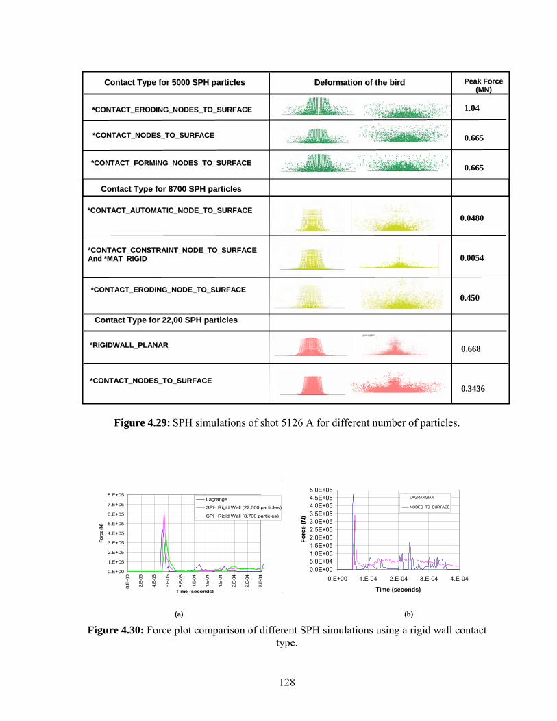
128
Figure 4.29: SPH simulations of shot 5126 A for different number of particles.
Figure 4.30: Force plot comparison of different SPH simulations using a rigid wall contact type.
**CCOONNTTAACCTT__EERROODDIINNGG__NNOODDEESS__TTOO__SSUURRFFAACCEE
**CCOONNTTAACCTT__NNOODDEESS__TTOO__SSUURRFFAACCEE
**CCOONNTTAACCTT__FFOORRMMIINNGG__NNOODDEESS__TTOO__SSUURRFFAACCEE
CCoonnttaacctt TTyyppee ffoorr 55000000 SSPPHH ppaarrttiicclleess
**CCOONNTTAACCTT__AAUUTTOOMMAATTIICC__NNOODDEE__TTOO__SSUURRFFAACCEE
CCoonnttaacctt TTyyppee ffoorr 88770000 SSPPHH ppaarrttiicclleess
**CCOONNTTAACCTT__CCOONNSSTTRRAAIINNTT__NNOODDEE__TTOO__SSUURRFFAACCEE AAnndd **MMAATT__RRIIGGIIDD
**CCOONNTTAACCTT__EERROODDIINNGG__NNOODDEE__TTOO__SSUURRFFAACCEE
1.04 0.665
0.665
0.0480
0.0054
0.450
DDeeffoorrmmaattiioonn ooff tthhee bbiirrdd PPeeaakk FFoorrccee ((MMNN))
**RRIIGGIIDDWWAALLLL__PPLLAANNAARR
**CCOONNTTAACCTT__NNOODDEESS__TTOO__SSUURRFFAACCEE
0.668 0.3436
CCoonnttaacctt TTyyppee ffoorr 2222,,0000 SSPPHH ppaarrttiicclleess
0.0E+005.0E+041.0E+051.5E+052.0E+052.5E+053.0E+053.5E+054.0E+054.5E+055.0E+05
0.E+00 1.E-04 2.E-04 3.E-04 4.E-04
Time (seconds)
Forc
e (N
)
LAGRANGIAN
NODES_TO_SURFACE
0.E+00
1.E+05
2.E+05
3.E+05
4.E+05
5.E+05
6.E+05
7.E+05
8.E+05
0.E+
00
2.E-
05
4.E-
05
6.E-
05
8.E-
05
1.E-
04
1.E-
04
1.E-
04
2.E-
04
2.E-
04
2.E-
04
Time (seconds)
Forc
e (N
)
Lagrange
SPH Rigid Wall (22,000 particles)
SPH Rigid Wall (8,700 particles)
(a) (b)

129
It can be observed from Figs. 4.30(a) that the results for the peak force in the SPH simulation
with 22,000 particles were 96.5% higher than the SPH (8,700 particles) simulation. However,
the behavior after the initial impact is similar in both SPH simulations, reaching a value close
to zero. The high value of force obtained from the 22,000 particle simulation could be
because by adding more particles to the SPH simulation the results in more bounce off effect,
and the momentum of the first particles that impact the surface increase when impacting the
upcoming particles.
Figure 4.31: Comparison of peak pressure obtained in Lagrangian and SPH simulation using
the nodes to surface contact TEROD=1.1
0
10000
20000
30000
40000
50000
60000
70000
80000
SIMULAT
PEA
K
4,704 8,700 22,000 Number of SPH
*CONTACT ERODING NODE TO

130
Figure 4.31 shows a comparison between peak force for different number of particles and
type of contact used. It can be observed that the *CONTACT_ERODING_NODE_TO_
SURFACE and the in the *CONTACT _NODE_TO_SURFACE simulation with 8,700
particles have a peak pressure close to the peak pressure obtained in the Lagrangian
simulation (6.5% lower than the Lagrangian case). These contact types are then one of the
indicated to be used in SPH simulation of bird-strike because of its capability of reproduce
the loads in the impact close to the Lagrange model and to the test data.
Using the results obtained it is observed that the mesh density affects the simulation.
Simulated transducers make possible getting the pressure distribution graph. When two
different mesh resolutions are used, the results are more accurate with respect to the
maximum pressure obtained.
4.4 Impact for a Tapered Plate Impact at 0º Now, we verify our model with the simulations provided by Moffat et al. (2001). As
in the case of Lagrange simulation, we considered to different bird impact angles: 0º and 30º.
The dimension and properties of the tapered plate are identical to those of previous
simulations. The number of SPH particles created for this simulation was 26195 and its
distribution was arranged to form the cylinder. The contact type used for this simulation was
*CONTACT_ERODING_NODE_TO_ SURFACE. The impact angle was 0º, as shown in
Fig. 4.32.

131
Figure 4.32: Cross section of the model for tapered plate impact using a higher density of SPH particles.
Using Material Null
Figure 4.33 shows that the resultant force for this SPH simulation is approximately 0.0153
MN which represents an error of 7.74% if compared with the 0.0142 MN of the Lagrangian
case. The reason is that there is little interaction between the tapered plate and the bird which
is sliced in two parts. This is the same behavior observed in the Lagrangian approach. Only
few particles are involved in the impact for the SPH simulation. The results for the 0 degrees
of impact simulation show that there is an only slight deformation in the tapered plate. Also,
there was no appreciable deformation of the leading edge as can be observed in Figs. 4.34 to
4.36. Figure 4.34 shows that the particles aligned with the plate were the ones suffering
deflection while the other particles continued their trajectory. In short, for cases in which the
impact-event occurs in the thinnest side of a plate, the SPH model can be used to simulate
impact events.
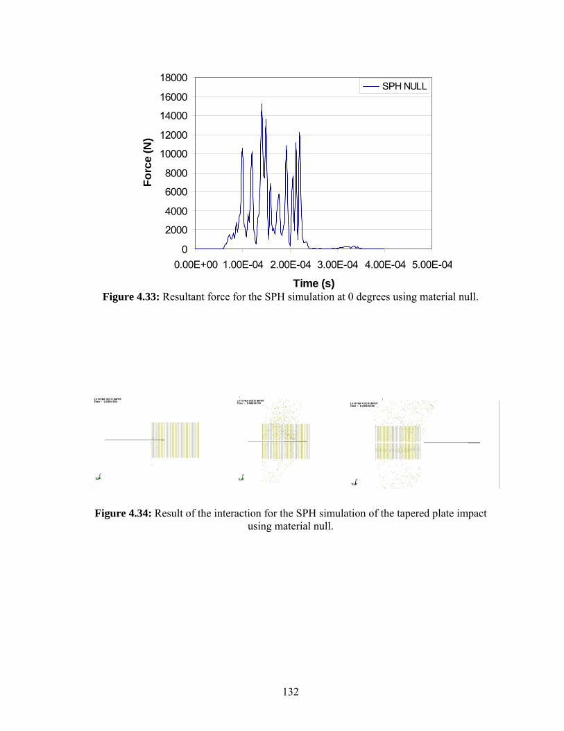
132
0
2000
4000
6000
8000
10000
12000
14000
16000
18000
0.00E+00 1.00E-04 2.00E-04 3.00E-04 4.00E-04 5.00E-04
Time (s)
Forc
e (N
)
SPH NULL
Figure 4.33: Resultant force for the SPH simulation at 0 degrees using material null.
Figure 4.34: Result of the interaction for the SPH simulation of the tapered plate impact
using material null.

133
Figure 4.35: Deformed plate after the 0 degrees impact of the SPH bird.
Figure 4.36: Front view of the deformed plate after the 0 degrees impact of the SPH bird using material null.
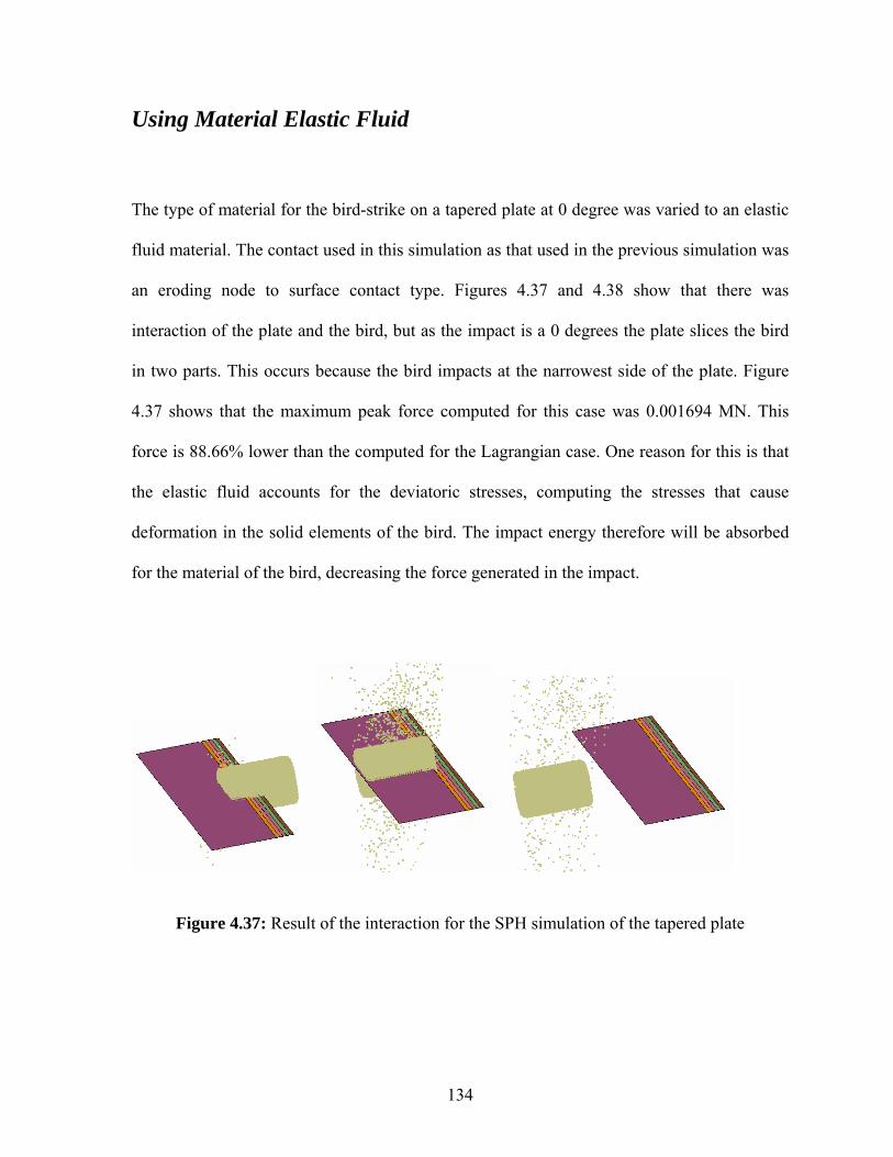
134
Using Material Elastic Fluid
The type of material for the bird-strike on a tapered plate at 0 degree was varied to an elastic
fluid material. The contact used in this simulation as that used in the previous simulation was
an eroding node to surface contact type. Figures 4.37 and 4.38 show that there was
interaction of the plate and the bird, but as the impact is a 0 degrees the plate slices the bird
in two parts. This occurs because the bird impacts at the narrowest side of the plate. Figure
4.37 shows that the maximum peak force computed for this case was 0.001694 MN. This
force is 88.66% lower than the computed for the Lagrangian case. One reason for this is that
the elastic fluid accounts for the deviatoric stresses, computing the stresses that cause
deformation in the solid elements of the bird. The impact energy therefore will be absorbed
for the material of the bird, decreasing the force generated in the impact.
Figure 4.37: Result of the interaction for the SPH simulation of the tapered plate

135
Figure 4.38: Front view of the deformed plate after the 0 degrees impact of the SPH bird
using material elastic fluid.
0.00E+00
2.00E+04
4.00E+04
6.00E+04
8.00E+04
1.00E+05
1.20E+05
0.E+00 5.E-05 1.E-04 2.E-04 2.E-04 3.E-04 3.E-04 4.E-04 4.E-04Time (s)
Forc
e (N
)
SPH 0 degfreesElastic fluid
Figure 4.39: Resultant force for the SPH simulation at 0 degrees using material elastic fluid.
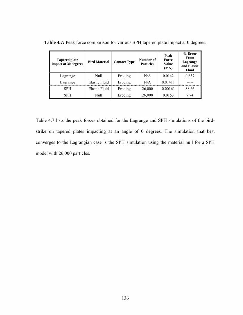
136
Table 4.7: Peak force comparison for various SPH tapered plate impact at 0 degrees.
Tapered plate impact at 30 degrees Bird Material Contact Type Number of
Particles
Peak Force Value (MN)
% Error From
Lagrange and Elastic
Fluid Lagrange Null Eroding N/A 0.0142 0.637 Lagrange Elastic Fluid Eroding N/A 0.01411 -----
SPH Elastic Fluid Eroding 26,000 0.00161 88.66 SPH Null Eroding 26,000 0.0153 7.74
Table 4.7 lists the peak forces obtained for the Lagrange and SPH simulations of the bird-
strike on tapered plates impacting at an angle of 0 degrees. The simulation that best
converges to the Lagrangian case is the SPH simulation using the material null for a SPH
model with 26,000 particles.

137
4.5 Impact for a Tapered Plate at 30º
The bird, simulated with the cylinder, was rotated by an angle of 30º as shown in Fig.
4.40. The variables and parameter were the same as in the simulation of section 4.4. The
contact used in this case was the *ERODING_NODE_TO_SURFACE. The influence of the
type of material used on the final force and deflection was studied. The materials used were
the null material and the elastic fluid material type.
Using Null material
The same model used in the impact at 0 degrees in which the amount of particles was 26,000
was used here. The type of material was the *MAT_NULL. Figure 4.41 shows the
deformation of the tapered plate at different times of the simulation. In this case, the
maximum normal deflection was 1.12 in which was 6.96% higher than the value obtained by
Moffat et al. (2001). This deflection is show in Fig. 4.42. The side view is shown in Fig.
4.43.
Figure 4.40: Side view of the SPH simulation for the bird impacting a plate at 30º.

138
Figure 4.41: Deformation of the tapered plate using material null and 26195 SPH particles.
Figure 4.42: Top view of the deformed plate after the impact of the bird with an angle of 30
degrees.
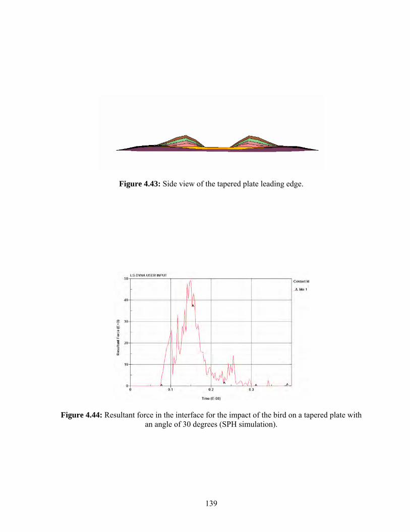
139
Figure 4.43: Side view of the tapered plate leading edge.
Figure 4.44: Resultant force in the interface for the impact of the bird on a tapered plate with
an angle of 30 degrees (SPH simulation).
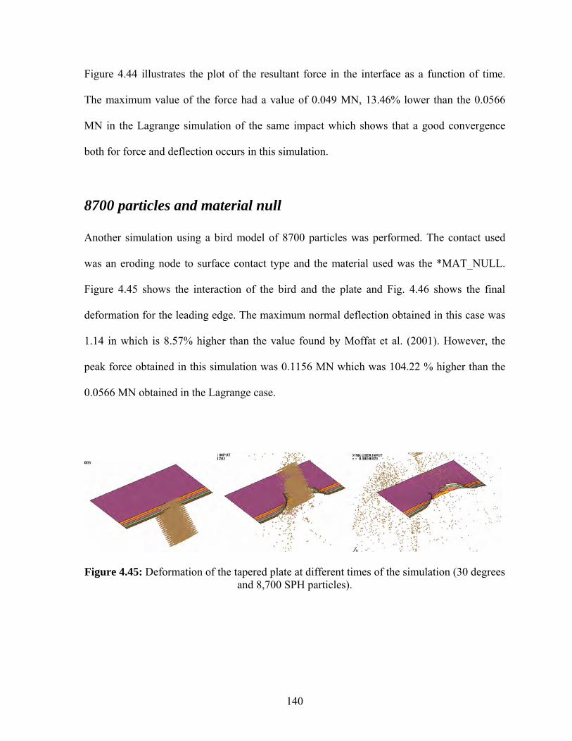
140
Figure 4.44 illustrates the plot of the resultant force in the interface as a function of time.
The maximum value of the force had a value of 0.049 MN, 13.46% lower than the 0.0566
MN in the Lagrange simulation of the same impact which shows that a good convergence
both for force and deflection occurs in this simulation.
8700 particles and material null
Another simulation using a bird model of 8700 particles was performed. The contact used
was an eroding node to surface contact type and the material used was the *MAT_NULL.
Figure 4.45 shows the interaction of the bird and the plate and Fig. 4.46 shows the final
deformation for the leading edge. The maximum normal deflection obtained in this case was
1.14 in which is 8.57% higher than the value found by Moffat et al. (2001). However, the
peak force obtained in this simulation was 0.1156 MN which was 104.22 % higher than the
0.0566 MN obtained in the Lagrange case.
Figure 4.45: Deformation of the tapered plate at different times of the simulation (30 degrees
and 8,700 SPH particles).

141
Figure 4.46: Top view of the deformed plate after the impact of the bird with an angle of 30 degrees and 8,700 particles.
26,000 SPH particles and Elastic Fluid material
For this simulation, the material type was changed in order to study its influence in the final
deflection of the leading edge and the peak force generated in the impact. The interaction of
the bird and the plate is depicted in Fig. 4.47. Figure 4.48 shows that the maximum normal
deflection was 1.25 in which is 19.6% higher than the 1.05 in found by Moffat et al. (2001).
Figure 4.49 shows that the peak force for this simulation was 0.109 MN and is 93.8 % higher
than the value obtained in the Lagrangian case. This increase in the force means that
changing the material type to an elastic fluid material will affect the value of the peak force,
as the type of equation of state is different.
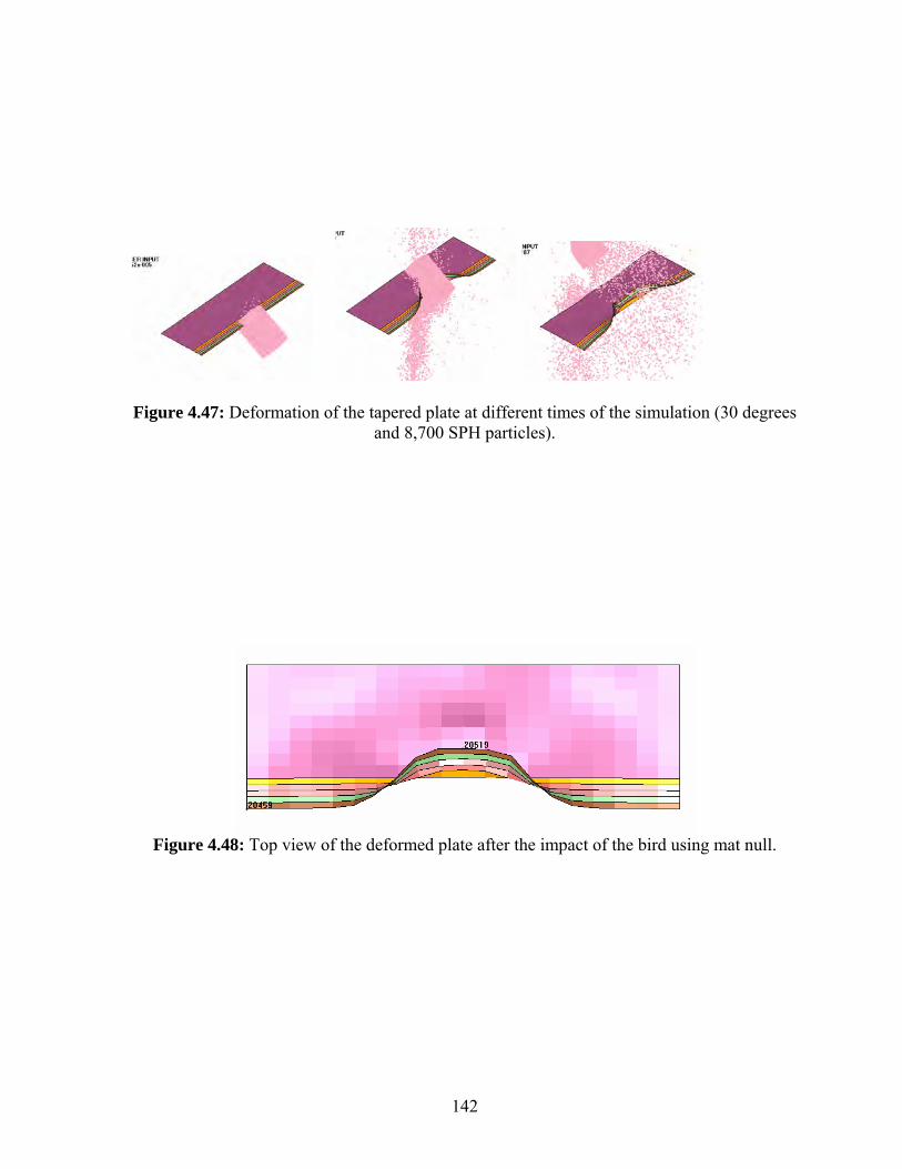
142
Figure 4.47: Deformation of the tapered plate at different times of the simulation (30 degrees
and 8,700 SPH particles).
Figure 4.48: Top view of the deformed plate after the impact of the bird using mat null.

143
Figure 4.49: Resultant force in the interface for the impact of the bird on a tapered plate with
an angle of 30 degrees (SPH simulation).
Table 4.8: Force and maximum normal deflection comparison for various SPH tapered plate impact at 30 degrees.
Tapered plate impact at 30 degrees Bird Material Contact Type Number of
Particles
Maximum Normal
Deflection (in)
% Error from
Moffat
Peak Force Value (MN)
Moffat N/A N/A N/A 1.05 N/A N/A Lagrange Null Eroding N/A 1.36 29.84 0.0537 Lagrange Elastic Fluid Eroding N/A 1.19 13.38 0.0566
SPH Elastic Fluid Eroding 26,000 1.25 19.61 0.1097 SPH Null Eroding 8,700 1.14 8.57 0.1156 SPH Null Eroding 26,000 1.12 6.96 0.0489

144
A observe in Table 4.8 the simulation that has better convergence to the maximum deflection
found by Moffat is the SPH simulation using material null and 26,000 particles. In addition,
for this model the peak force obtained was only 13.4% different from the one calculated
using the Lagrange simulation with material elastic fluid. But if the peak force is compared
with the Lagrangian case using the same null material the error is 8.93%. However, changing
the material in the SPH simulation to the material elastic fluid does not result in a
convergence of the force to the Lagrangian model using the same elastic fluid material.
4.6 Computational Time Employed
The time employed in the simulation of the bird-strike using the Lagrangian and SPH
methods are presented in this chapter. Three different cases of impact were analyzed: Frontal
bird-strike impact in a flat circular rigid plate, bird-strike in a tapered plate at an angle of 30
degrees and finally bird-strike impact in a tapered plate at an angle of 0 degrees. Fig. 4.50
show the elapsed time for the different methods and impacts simulated.
99
271
43
1336
48
1868
0 200 400 600 800 1000 1200 1400 1600 1800 2000
Lagrange
SPH
Time (seconds)
Fontal Impact-Circular Rigid-Plate Tapered plate at 30 Degrees Tapered plate at 0 Degrees
Figure 4.50: Elapsed simulation time for Lagrange and SPH methods and impact types.

145
4.7 Comparison of the Total Energy
Frontal Bird Strike Impact in a Flat Circular Rigid-Plate
In order to further analyze the results obtained, energy plots were created in LS-
DYNA for Lagrangian and SPH simulations. Figure 4.51 shows the superposition of the
total, kinetic, and internal energy for the Lagrange and SPH simulation with the specified
number of particles and types of contacts. It can be observed that the total energy increases
for the SPH simulations while it decreases for the Lagrangian simulations. The reason is that
in the Lagrangian simulation there is an energy loss due to the friction of the whole bird
model with the plate. This friction can be observed in the deformation of the Lagrangian
simulations.
0.0E+00
2.0E+03
4.0E+03
6.0E+03
8.0E+03
1.0E+04
1.2E+04
1.4E+04
1.6E+04
1.8E+04
0.0E+00
3.6E-05
7.2E-05
1.1E-04
1.4E-04
1.8E-04
2.2E-04
2.5E-04
2.9E-04
3.2E-04
3.6E-04
4.0E-04
TIME (SECONDS)
ENER
GY
(LB
F-IN
)
LAGRANGE ERODING NODES TOSURFACE
SPH 10,000 PARTICLES AND NODES TOSURFACE
SPH 5,000 PARTICLES NODES TOSURFACE
INTERNAL ENERGY LAGRANGE
KINETIC ENERGY LAGRANGE
INTERNAL ENERGY 5000 SPH PARTICLES
KINETIC ENERGY 5000 SPH PARTICLES
INTERNAL ENERGY 10,000 SPHPARTICLES
KINETIC ENERGY 10,000 SPH PARTICLES
"KINETIC ENERGY 2000 SPH PARTICLES
INTERNAL ENERGY 2,000 SPH PARTICLES
SPH 2,000 PARTICLES AND NODES TOSURFACE
Figure 4.51: Plot of the total, internal, and kinetic energy for the SPH and Lagrangian
simulations
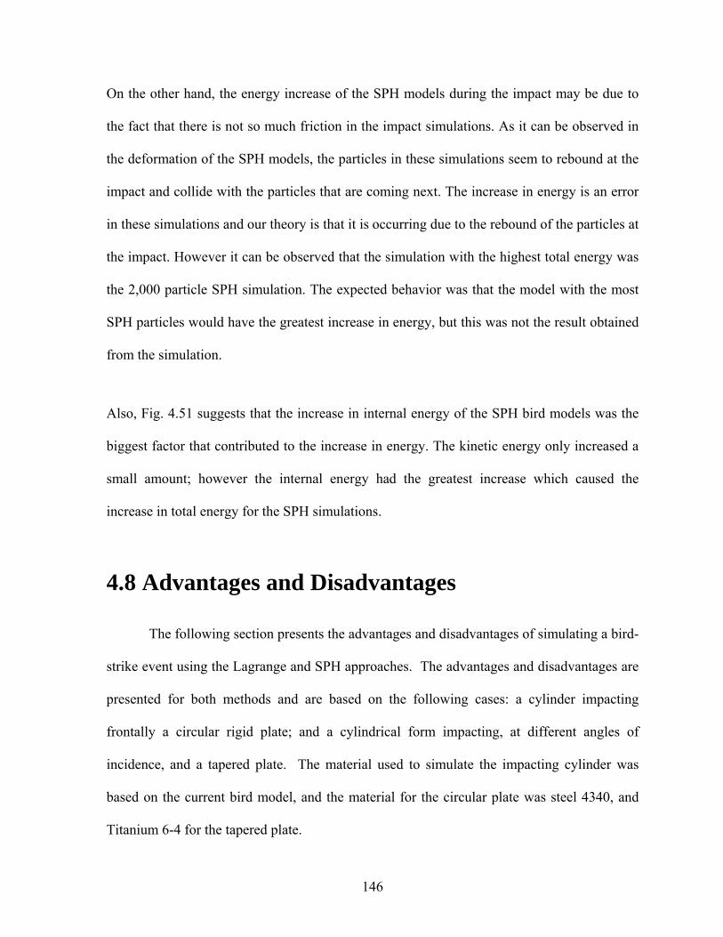
146
On the other hand, the energy increase of the SPH models during the impact may be due to
the fact that there is not so much friction in the impact simulations. As it can be observed in
the deformation of the SPH models, the particles in these simulations seem to rebound at the
impact and collide with the particles that are coming next. The increase in energy is an error
in these simulations and our theory is that it is occurring due to the rebound of the particles at
the impact. However it can be observed that the simulation with the highest total energy was
the 2,000 particle SPH simulation. The expected behavior was that the model with the most
SPH particles would have the greatest increase in energy, but this was not the result obtained
from the simulation.
Also, Fig. 4.51 suggests that the increase in internal energy of the SPH bird models was the
biggest factor that contributed to the increase in energy. The kinetic energy only increased a
small amount; however the internal energy had the greatest increase which caused the
increase in total energy for the SPH simulations.
4.8 Advantages and Disadvantages The following section presents the advantages and disadvantages of simulating a bird-
strike event using the Lagrange and SPH approaches. The advantages and disadvantages are
presented for both methods and are based on the following cases: a cylinder impacting
frontally a circular rigid plate; and a cylindrical form impacting, at different angles of
incidence, and a tapered plate. The material used to simulate the impacting cylinder was
based on the current bird model, and the material for the circular plate was steel 4340, and
Titanium 6-4 for the tapered plate.
147
Lagrangian Approach
The Lagrange FEA method presented the following advantages when compared to the
SPH method:
1. Noticeable reduction in computational time
2. The development of the whole model (construction and assignation of variables) is
simpler than the SPH and ALE method.
3. More defined shapes can be achieved when simulating an object.
4. Simulation variables are constant during different types of simulations, for example:
This method permits the simulation of impact events in situations where the impacts
occur in the narrowest part of a plate.
5. Material simulated is a continuum
The Lagrange FEA method presented the following disadvantages when compared to the
SPH method:
1. Element (mass) loss during simulation
2. Noticeable loss on total energy
3. Deformation is not uniform due to the loss of elements
4. Resultant force graphs are not as uniform as those produced using the SPH method
Smoothing Particle Hydrodynamics Approach
The SPH method is a relatively a new finite element method. For studies involving
impact events this method simulates the material, which has the largest deformation when the
impact is occurring, as a mesh of individual particles that interact among them when a great
148
external force, that creates large deformations, acts on them. Following are some of the
advantages for the SPH method:
1. In impact Events there is no loss or change in mass
2. Distribution of resultant force along time is more uniform and approaches the
behavior observed in the Barber et al. (1975) research
3. The number of variables that affect the final result of the simulation is reduced to just
contact variables and variables related to the SPH control card
4. In both methods total energy loss occurred, but the SPH method presents the lowest
change
Following are some of the disadvantages for the SPH method:
1. Material is not continuous
2. Greater computational time compared with the Lagrange method
3. More complicated model development when compared to the Lagrange modeling,
object shapes are more difficult to achieve
4. Impacts occurring on the narrowest part of the plate require a mesh with a great
number of elements, increasing simulation time. The increasing in mesh density does
not assure that particles interact with the plate; there could be no interaction because
of the gap between the particles
5. Contact type changes depending on the impact event to be simulated

149
4.9 Best Approach for Bird-Strike Event Modeling
After studying the influence of various parameters involved in the SPH bird model,
we compared the peak pressure and we are ready to make some recommendation on when is
it best to use this approach. First and foremost, the SPH bird model is far more complex than
the Lagrangian bird model and the number of variables influencing the SPH model is higher
than for the Lagrangian one. For the SPH bird model, the mesh density or number of particles
included has a strong influence in the peak impact pressure. This causes the selection of an
optimum number of particles before beginning further simulations.
For the first case, the frontal impact against a flat rigid plate, a bird model with 8700 particles
with one-way constraint contact type and a null material type can be used. The error obtained
in the pressure after comparing with the experimental data is within 10%. For the Lagrangian
model the error when using elastic fluid material and an eroding contact type produced and
error of 9%. Therefore, the SPH model can successfully be used in this kind of frontal
impacts.
For the second case, 0 and 30 degrees impact against a tapered plate, the SPH model
validates the results obtained in the literature. The SPH model is recommended for angled
impacts on tapered plates since the error of the maximum normal deflection in less than 7%
when compared with the experimental data by Moffat et al. (2001). These results are
validated using 26,000 SPH particles, a eroding contact type and a null material. If compared
with the Lagrangian simulation in which the error was 13.3% when using an elastic fluid
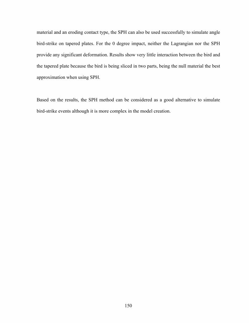
150
material and an eroding contact type, the SPH can also be used successfully to simulate angle
bird-strike on tapered plates. For the 0 degree impact, neither the Lagrangian nor the SPH
provide any significant deformation. Results show very little interaction between the bird and
the tapered plate because the bird is being sliced in two parts, being the null material the best
approximation when using SPH.
Based on the results, the SPH method can be considered as a good alternative to simulate
bird-strike events although it is more complex in the model creation.
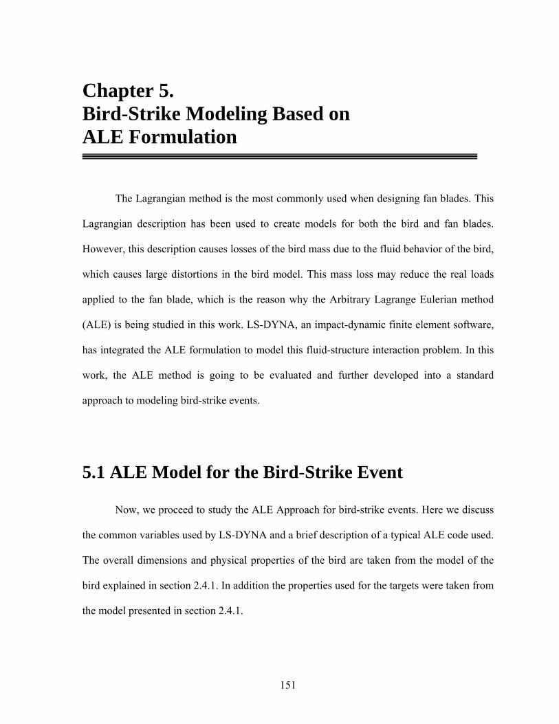
151
Chapter 5. Bird-Strike Modeling Based on ALE Formulation
The Lagrangian method is the most commonly used when designing fan blades. This
Lagrangian description has been used to create models for both the bird and fan blades.
However, this description causes losses of the bird mass due to the fluid behavior of the bird,
which causes large distortions in the bird model. This mass loss may reduce the real loads
applied to the fan blade, which is the reason why the Arbitrary Lagrange Eulerian method
(ALE) is being studied in this work. LS-DYNA, an impact-dynamic finite element software,
has integrated the ALE formulation to model this fluid-structure interaction problem. In this
work, the ALE method is going to be evaluated and further developed into a standard
approach to modeling bird-strike events.
5.1 ALE Model for the Bird-Strike Event
Now, we proceed to study the ALE Approach for bird-strike events. Here we discuss
the common variables used by LS-DYNA and a brief description of a typical ALE code used.
The overall dimensions and physical properties of the bird are taken from the model of the
bird explained in section 2.4.1. In addition the properties used for the targets were taken from
the model presented in section 2.4.1.
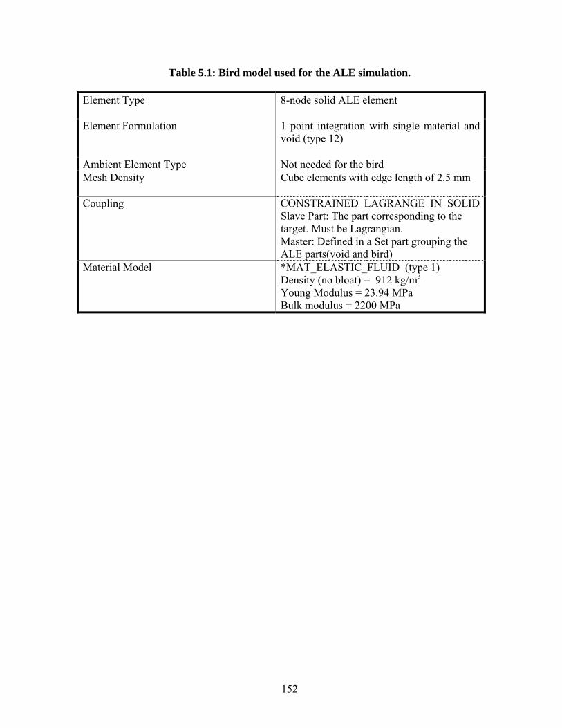
152
Table 5.1: Bird model used for the ALE simulation.
Element Type 8-node solid ALE element
Element Formulation 1 point integration with single material and void (type 12)
Ambient Element Type Not needed for the bird Mesh Density Cube elements with edge length of 2.5 mm
Coupling CONSTRAINED_LAGRANGE_IN_SOLID
Slave Part: The part corresponding to the target. Must be Lagrangian. Master: Defined in a Set part grouping the ALE parts(void and bird)
Material Model *MAT_ELASTIC_FLUID (type 1) Density (no bloat) = 912 kg/m3 Young Modulus = 23.94 MPa Bulk modulus = 2200 MPa

153
5.1.1 Pre-Processing in the ALE Formulation
When modeling a bird-strike event using the ALE description it is necessary to create
a void mesh surrounding the bird. Both the void and the bird must be part of one
computational domain and the elements do not have to overlap. Therefore, it is necessary to
merge the common nodes of the bird and the surrounding mesh (Goyal et al., 2006b). The
ALE bird model uses parameters in Table 5.1.
5.2 Bird Impact Against a Flat Plate The bird-strike simulations in a flat rigid plate are based on the shot 5126A by the
Barber et al. (1975), as previously discussed in Chapters 3 and 4. The purpose of the
simulations performed here is an attempt to incorporate the ALE approach for bird-strike
events, and thus validate results with the experimental data and the Lagrange model. LS-
DYNA data output parameters such as *DATABASE_FSI are used to obtain the impact
force and average pressure diagrams.
Two different simulations were performed: 2D and 3D ALE cases of the impact of a
bird against a rigid plate. The first one is a 2D simulation based on the work done by Souli
and Olovsson (2000), which has been validated and proven to be a reliable method. The
second model is a 3D simulation to study the bird strike event in solid rigid plates studied by
Barber et al (1975).

154
5.2.1 Bird Strike Simulation Using 2D ALE
Let us begin with the 2D ALE model. First, we varied the coupling and reference
system parameters inside the *CONSTRAINT_LAGRANGE_IN_SOLID and *ALE_
REFERENCE_SYSTEM_GROUP cards. By studying the deformations, the best results are
achieved when we take a reference system type parameter of PRTYPE=5 and a coupling type
parameter of CTYPE=5.
Here, we set the initial velocity of the model to 198 m/s (442.9 mph), which is the velocity
used in the Lagrange simulation. This velocity is assigned to a node set containing the bird
and the void mesh using the *INITIAL_VELOCITY card. A node set containing all the
nodes of the plate is created, where all degrees of freedom are constraints to model the flat
rigid plate. A moving mesh was simulated without constraints of expansion. The material
used for the target was the *MAT_PLASTIC_KINEMATIC and for the bird and void the
*MAT_ELASTIC_FLUID. A penalty coupling was used to specify the type of coupling
inside the *CONSTRAINED_LAGRANGE_IN_SOLID card. Figure 5.1 shows the
interaction between the bird and the shell and the moving reference for the void mesh. The
void has no constraints of rotation about the z axis.
The impacting progression for this simulation can be observed in Fig. 5.1. It can be observed
that the modeled bird deforms to the sides although there is no a complete sliding of all of the
bird material on the target. The mesh deforms as the bird impacts the target. The reference
system follows an automatic mesh motion following a mass weighted average velocity in
ALE.
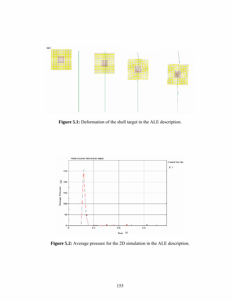
155
Figure 5.1: Deformation of the shell target in the ALE description.
Figure 5.2: Average pressure for the 2D simulation in the ALE description.
(N)
(s)

156
As observed in Fig. 5.2, the maximum pressure obtained in this ALE simulation is
approximately 3.5 MPa. The model used in this simulation has smaller dimensions than the
dimensions of the bird tested by Barber in shot 5126A and for this reason it was not expected
to produce the same results as in the test data. However, the behavior of the pressure between
the fluid and the structure is similar to that observed in both Lagrange simulations and
experimental data by Barber et al. (1975). Once again, the steady state for this case is not as
well captured; instead the zero value is obtained after a short period of time.
The maximum force obtained for this ALE simulation is 0.080 MN in the negative x
direction. This result can not be compared with the Lagrange simulation because the
geometrical models in both cases are not the same. The variables used in the ALE cards for
this case will be used as reference to create an ALE model that fits the geometrical
dimensions of a bird strike performed by Barber et al. (1975), specifically shot 5126 A.
5.2.2 2D ALE Simulation of Shot 5126A
By changing various bird parameters, a new deformation for the model bird is
created. The deformation is shown in Fig. 5.3. The reference system composed by the
surrounding void mesh translates following an automatic mesh motion using mass weighted
average velocity. The NADV variable (Number of cycles between advections) was changed
to the flag of 1 in the *CONTROL_ALE card.

157
Figure 5.3: Deformation of the 2D ALE bird impacting a rigid plate.
Figure 5.4: Average pressure (left) and force in the negative x direction (right) for ALE
simulation using NADV=1
(N)
(s)
(N)
(s)

158
Figure 5.4 shows the average pressure and force in the x direction. The peak pressure is
approximately 36 MPa, which is 10% lower than the 40 MPa measured by Barber et al.
(1975) and 17.54% lower than the 43.66 MPa obtained from the Lagrangian formulation
using the elastic fluid material. In this case there is almost no variation in the impact area
when compared with the SPH and Lagrange methods. Also, in the ALE method there is no
change in the global mass of the model as in the Lagrange method. This is observed in Fig.
5.5, which shows zero change in the mass, in contrast with the Lagrange model shown in Fig.
3.4. This suggests that the loads generated with the ALE method could be more accurate to
the real loads generated in a bird-strike event. This also is supported by the fact that the peak
pressure obtained in the ALE method was 10% of the test data obtained by Barber et al.
(1975).
Figure 5.5: Change in mass for the 2D ALE simulation
(Ton
)
(s)

159
Figure 5.6: Pressure contours for the ALE simulation using NADV=1
Figure 5.6 shows the pressure contour progression for this simulation at different times of the
impact. The fringe levels of pressure for the first impact of the bird are show in Fig. 5.6. The
fringe levels changes from one plot to another in different time intervals. As observed in this
figure, a shock pressure is generated at the moment of the impact. This shock pressure travels
from the front to the back of the simulated ALE bird. The red elements represent the zone of
higher pressure for each of the plots presented in Fig. 5.6. The highest value obtained was
278 MPa. This is the pressure calculated for one ALE element inside of the modeled bird and
does not necessarily represent the pressure exerted on the target. The pressure contours
confirm that the compressive shock waves, shown by Cassenti (1979), are also calculated by
the 2D ALE simulation of a bird-strike.

160
5.2.3 Bird Strike Simulation Using ALE in 3D
A three dimensional ALE model in LS-DYNA of shot 5126A Barber et al. (1975) is
also created. The simulation is performed by creating a void mesh inside of the bird. The
dimensions and parameters were those corresponding to shot 5126 A. The material used for
the bird was the *MAT_ELASTIC_FLUID and *MAT_PLASTIC_KINEMATIC for the
plate. The formulation used for the ALE bird and surrounding void mesh simulation was the
one-point integration with single material and void.
Figure 5.7 shows the meshing of the void material for this simulation. Also the merged nodes
on the common boundaries of the void and the cylinder can be observed. This is a necessary
condition to allow the bird material to flow through the void mesh. The number of cycles
between advection (NADV) variable inside the *CONTROL_ALE was set to one. The
continuum treatment used for this simulation was DCT = 2 (EULERIAN).
Figure 5.7: Meshing of the ALE simulation of Shot 5126 A
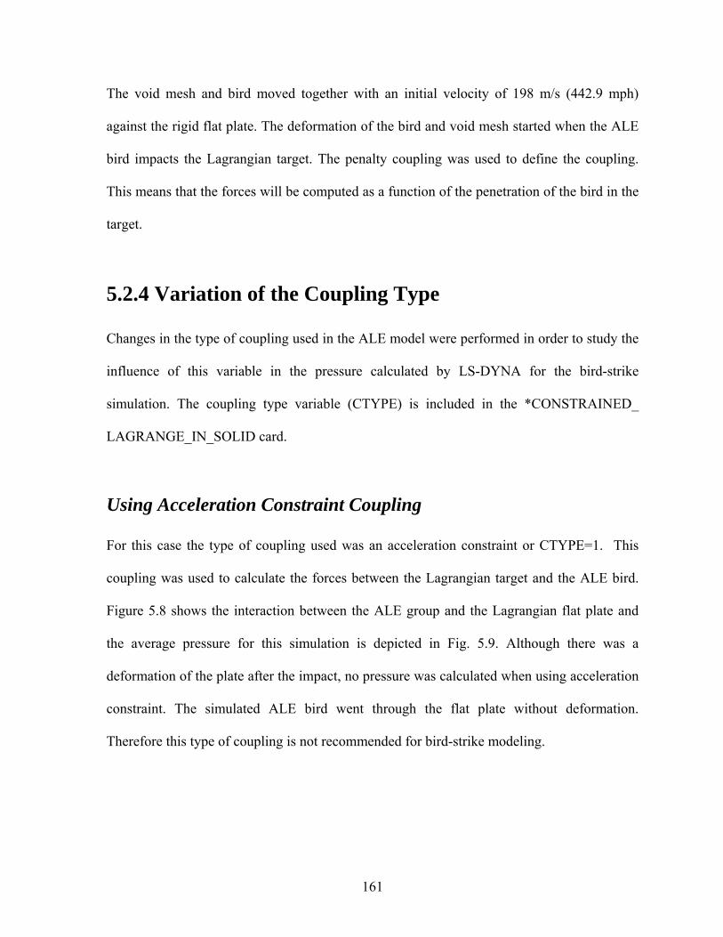
161
The void mesh and bird moved together with an initial velocity of 198 m/s (442.9 mph)
against the rigid flat plate. The deformation of the bird and void mesh started when the ALE
bird impacts the Lagrangian target. The penalty coupling was used to define the coupling.
This means that the forces will be computed as a function of the penetration of the bird in the
target.
5.2.4 Variation of the Coupling Type
Changes in the type of coupling used in the ALE model were performed in order to study the
influence of this variable in the pressure calculated by LS-DYNA for the bird-strike
simulation. The coupling type variable (CTYPE) is included in the *CONSTRAINED_
LAGRANGE_IN_SOLID card.
Using Acceleration Constraint Coupling
For this case the type of coupling used was an acceleration constraint or CTYPE=1. This
coupling was used to calculate the forces between the Lagrangian target and the ALE bird.
Figure 5.8 shows the interaction between the ALE group and the Lagrangian flat plate and
the average pressure for this simulation is depicted in Fig. 5.9. Although there was a
deformation of the plate after the impact, no pressure was calculated when using acceleration
constraint. The simulated ALE bird went through the flat plate without deformation.
Therefore this type of coupling is not recommended for bird-strike modeling.

162
Figure 5.8: ALE simulation with acceleration constrain.
Figure 5.9: Average pressure for the ALE simulation using acceleration constrain for the
coupling.
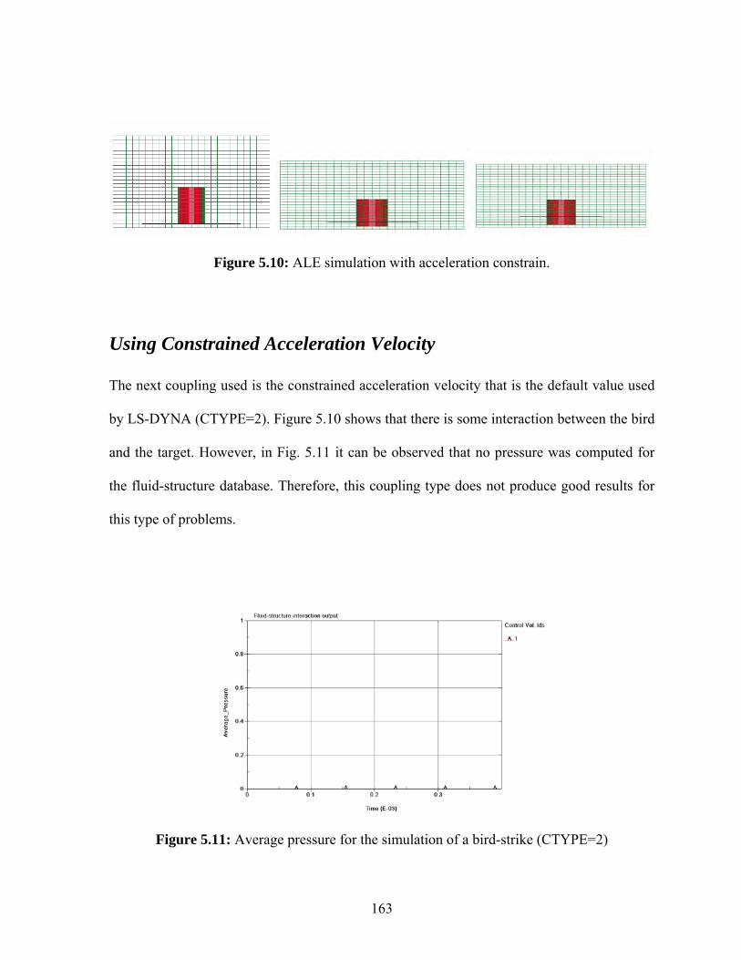
163
Figure 5.10: ALE simulation with acceleration constrain.
Using Constrained Acceleration Velocity
The next coupling used is the constrained acceleration velocity that is the default value used
by LS-DYNA (CTYPE=2). Figure 5.10 shows that there is some interaction between the bird
and the target. However, in Fig. 5.11 it can be observed that no pressure was computed for
the fluid-structure database. Therefore, this coupling type does not produce good results for
this type of problems.
Figure 5.11: Average pressure for the simulation of a bird-strike (CTYPE=2)

164
Figure 5.12: ALE simulation with an acceleration velocity constrain in the
*CONSTRAINED_LAGRANGE_IN_SOLID card.
Using Constrained Acceleration Velocity in the Normal direction
For this simulation the coupling type used was an acceleration velocity constraint in normal
direction only (CTYPE=3) for the coupling between the ALE bird and the Lagrangian target.
As seen in Fig. 5.12 the bird went deforms after the coupling, however Fig.5.13 shows that
there was no pressure in for the fluid-structure interaction database.
Figure 5.13: Average pressure for the simulation of a bird-strike (CTYPE =3)

165
Using Penalty Coupling without Erosion
The next coupling type used was the penalty coupling (CTYPE=4). The final shape of the
deformed bird for this case encloses the same behavior to that obtained in the 2D ALE
simulation as seen in Fig. 5.14. The deformation for this simulation was not as accurate as
desired and as a consequence the pressure in the coupling interface registered an approximate
value of 95 MPa as seen in Fig. 5.15. This value is 135% higher than the 40 MPa measured
in the test data corresponding to shot 5126A from Barber et al. (1975) and 117% higher to
the 43.6 MPa of the Lagrangian case. The reason is that the equation of state is a function of
time and thus the time step scale factor (TSSFAC) needs to be changed.
Figure 5.14: Deformation of the bird for the ALE simulation.

166
Figure 5.15: Average pressure for the 3D ALE simulation of the bird-strike
Based in the results obtained, the recommended coupling type when simulating bird-strike
events is the penalty based. For this coupling the forces are computed as a function of the
penetration of the ALE bird in the Lagrangian target. The acceleration and velocity constraint
coupling did not produced desired results.
5.2.4 Variation of the Time Step Scale Factor
The Time Step Scale Factor (TSSFAC) inside the *CONTROL_TIMESTEP was modified in
order to change the time step used for the ALE calculations. It is desired to study how this
variation affects the final results in the time history force and pressure generated by the fluid
structure database output.
The TSSFAC used in the previous 3D ALE simulation was 0.35 which produced a peak
pressure of 95 MPa, as seen in Fig. 5.15. A value of TSSFAC of 0.58 produced similar
(s)
(MPa
) Peak pressure: 95 MPa
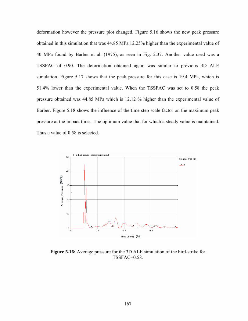
167
deformation however the pressure plot changed. Figure 5.16 shows the new peak pressure
obtained in this simulation that was 44.85 MPa 12.25% higher than the experimental value of
40 MPa found by Barber et al. (1975), as seen in Fig. 2.37. Another value used was a
TSSFAC of 0.90. The deformation obtained again was similar to previous 3D ALE
simulation. Figure 5.17 shows that the peak pressure for this case is 19.4 MPa, which is
51.4% lower than the experimental value. When the TSSFAC was set to 0.58 the peak
pressure obtained was 44.85 MPa which is 12.12 % higher than the experimental value of
Barber. Figure 5.18 shows the influence of the time step scale factor on the maximum peak
pressure at the impact time. The optimum value that for which a steady value is maintained.
Thus a value of 0.58 is selected.
Figure 5.16: Average pressure for the 3D ALE simulation of the bird-strike for
TSSFAC=0.58.
(s)
(MPa
)

168
Figure 5.17: Average pressure for the 3D ALE simulation of the bird-strike for
TSSFAC=0.90.
Pressure vs TSSFAC
0
20
40
60
80
100
0.3 0.5 0.7 0.9TSSFAC
Pres
sure
(MPa
)
Figure 5.18: Average pressure for the 3D ALE simulation of the bird-strike
(s)
(MPa
)

169
Table 5.2: Comparison of peak pressure for different Lagrange, SPH and ALE simulations.
CONTACT TYPE
TSSFAC
PEAK PRESSURE
VALUE (MPa)
%ERROR from the
TEST DATA
TEST DATA BY BARBER ET AL. (1975) N/A N/A 40 ---
LAGRANGE MAT ELASTIC FLUID ERODING CONTACT Lagrange N/A 43.66 9.15
SPH CONSTRAINT Using Simulated Transducer SPH N/A 37.3 6.75
2D ALE (PENALTY COUPLING) SHOT 5126 A, NADV=1 ALE 0.35 36 10
3D ALE MAT ELASTIC FLUID ALE 0.35 95 135
3D ALE MAT ELASTIC FLUID ALE 058 44.8 12
3D ALE MAT ELASTIC FLUID ALE 0.67 26.5 33.7
3D ALE MAT ELASTIC FLUID ALE 0.71 26.08 34.8
3D ALE MAT ELASTIC FLUID ALE 0.90 19.44 51.4
Table 5.2 shows the comparison of the average peak pressure generated for each of the ALE
simulation with the test data from Barber et al. (1975). As observed when the TSSFAC is
increased from the original value of 0.35 it considerably decrease the error compared with
the test data. The optimum value of the pressure in which the error was the lowest possible,
12%, was obtained when the TSSFAC was 0.58. Therefore, it can be concluded that for
simulation of bird-strike using the ALE method in 3D a value of 0.58 should be used for the
TSSFAC.

170
0.0
5.0
10.0
15.0
20.0
25.0
30.0
35.0
40.0
45.0
50.0
3.00E-05 8.00E-05 1.30E-04 1.80E-04 2.30E-04 2.80E-04
Time (s)
Pres
sure
(M
pa)
Lagrange Elastic Fluid2D ALE3D TSSFCA 0.673D ALE TSSFAC 0.58SPH Constraint
Figure 5.19: Pressure comparison for different ALE simulations
Figure 5.19 shows the comparison for the simulations performed using ALE, Lagrange and
SPH methods. Only selected cases are shown in this plot. The values corresponding to the
peak pressures are those shown in Table 5.2. The error for the Lagrange and SPH simulations
are under 10% and for the 3D ALE simulation with TSSFAC the error obtained was 12%.
The material used for the Lagrange and ALE is the elastic fluid and for the SPH was material
null. The peak pressure using the 2D ALE case has a delay which is irrelevant because it only
depends on the time that takes the bird to impact the plate which is a function of the distance
in which the bird was placed initially.

171
5.3 Bird-strike simulation in tapered plate
5.3.1 Simulation for Tapered Plate Impact at 0°
Now, we model a bird striking a tapered plate as was in the case of the Lagrangian model and
SPH model. The bird properties and the tapered plate are taken as the explained in section
2.3.2. Two different impact angles for tapered plate are considered: 0 degrees and 30 degrees.
The material used for the bird model is *MAT_ELASTIC_FLUID with a penalty coupling.
The variables for the *REFERENCE_SYSTEM_GROUP were kept the same as in previous
simulations.
2D Simulation
First a 2D simulation of the impact of the bird against the tapered plate was performed. The
coupling of the bird and the tapered plate needs to be calculated in all the directions. This
can be obtained setting the value of the DIREC variable inside the
*CONSTRAINT_LAGRANGE_IN_SOLID to 3. The type of coupling used in this
simulation was the penalty coupling (CTYPE=4). Figure 5.20 shows the interaction of the
bird and the plate. The peak force obtained was 0.01461 MN with an error of 1.4% if
compared with the Lagrangian simulation of the same case. The force plot is depicted in Fig.
5.21. It can observed that the bird did not go through the plate but

172
Figure 5.20: Interaction of he bird and the plate for 2D impact at 0 degrees.
ALE 2D
0
2000
4000
6000
8000
10000
12000
14000
16000
0.00E+00 1.00E-04 2.00E-04 3.00E-04 4.00E-04 5.00E-04
Time (s)
Forc
e (N
)
ALE 2D
Figure 5.21: Force plot for the 2D ALE simulation of the tapered plate impact at 0 degrees.

173
3D Simulation
The results obtained in the ALE simulation of a bird-strike impact against a tapered plate at 0
degrees were similar to that of the Lagrange and SPH cases. Figure 5.22 shows the
interaction of the bird and the plate. As expected, the bird was sliced in two parts and the
plate was slightly deformed as seen in Fig. 5.23. However the pressure plot generated by the
*DATABASE_FSI shows that there were little interaction between the Lagrangian plate and
the ALE bird. It was necessary to vary the penalty factor in this simulation in order to
calibrate the value of the force calculated in the coupling. The penalty factor (PFAC) is used
only when a penalty coupling type is included in the keyword. The PFAC variable scales the
estimated stiffness of the interacting (coupling) system. A value of 860 was used in our case
which was found to be the optimum value. Figure 5.24 shows the plot of the average pressure
in which the maximum value was 0.0112 MN, 20.4% lower than the 0.0141 MN computed
by the Lagrange case using material elastic fluid.
Figure 5.22: ALE Bird impacting a tapered plate at 0 degrees at different time intervals and
the top view of the tapered plate after the impact.

174
Figure 5.23: Frontal view of the deformation of the tapered plate.
0
2000
4000
6000
8000
10000
12000
0.00E+00 1.00E-04 2.00E-04 3.00E-04 4.00E-04 5.00E-04
Time (s)
Forc
e (N
)
2D ALE 0 deg pfac860
Figure 5.24: Force plot for the ALE simulation of a tapered plate bird-strike for a 0 degrees
impact.

175
5.3.2 ALE Simulation for Tapered Plate Impact at 30°
2D Simulation
The same model of the 2D bird used in section 5.3.1 was used here with the difference that it
was rotated an angle of 30 degrees as shown in Fig. 5.25. The maximum deflection for this
case was measured to be 1.18 in, 11.9% higher than the value obtained by Moffat et al
(2001). Figure 5.26 shows that the maximum force obtained in this simulation was 0.05319
MN which is 6.06% higher than the Lagrange case. This value was obtained using a penalty
coupling with a penalty factor of 120.
Figure 5.25: ALE Bird impacting a tapered plate at 0 degrees at different time intervals

176
0
10000
20000
30000
40000
50000
60000
0.00E+00
5.00E-05
1.00E-04
1.50E-04
2.00E-04
2.50E-04
3.00E-04
3.50E-04
4.00E-04
Time (s)
Forc
e (N
)
2D ALE 30 DEG
Figure 5.26: Force plot for the 2D ALE simulation of the tapered plate impact at 30 degrees.
3D Simulation
Here a 3D simulation of the bird impact at 30 degrees against the deformable tapered
plate is performed. Figure 5.16 shows the interaction of the ALE bird with the Lagrangian
plate for different time intervals. Comparing Fig. 3.19 and 5.27, we observe that the
deformation in the ALE simulation has a similar behavior as in the Lagrangian case. The
maximum normal deflection shown in Fig. 5.28 for this ALE simulation was 1.25 in which is
19.8 % higher than the value found by Moffat et al. (2001) and 5.65 % lower than the
Lagrange case using elastic fluid material. In addition, the ALE bird suffered a little change
in dimensions only without any loss of mass.
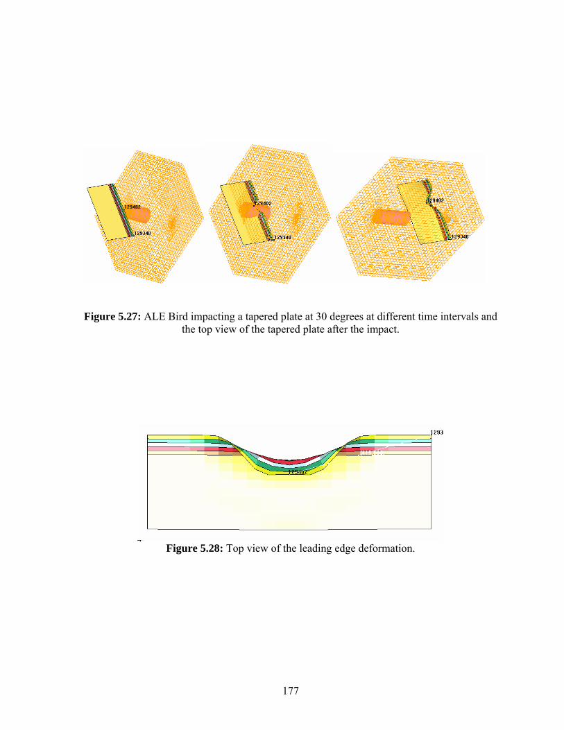
177
Figure 5.27: ALE Bird impacting a tapered plate at 30 degrees at different time intervals and
the top view of the tapered plate after the impact.
Figure 5.28: Top view of the leading edge deformation.
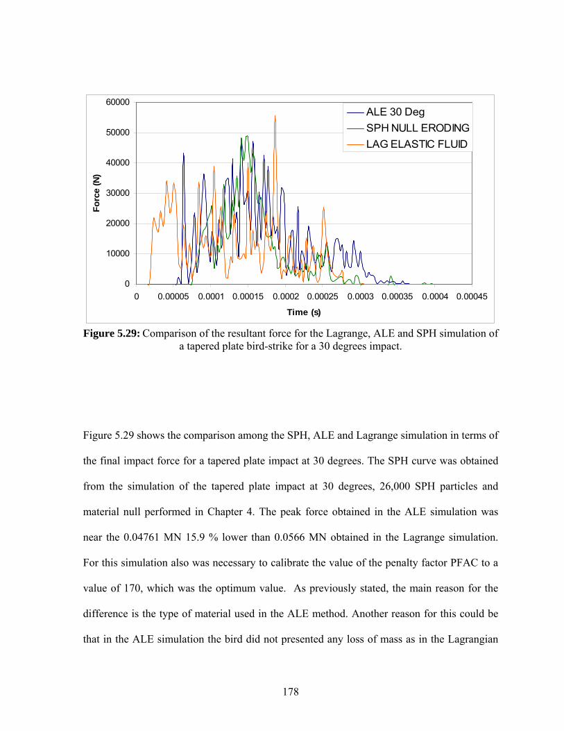
178
0
10000
20000
30000
40000
50000
60000
0 0.00005 0.0001 0.00015 0.0002 0.00025 0.0003 0.00035 0.0004 0.00045
Time (s)
Forc
e (N
)
ALE 30 DegSPH NULL ERODINGLAG ELASTIC FLUID
Figure 5.29: Comparison of the resultant force for the Lagrange, ALE and SPH simulation of
a tapered plate bird-strike for a 30 degrees impact.
Figure 5.29 shows the comparison among the SPH, ALE and Lagrange simulation in terms of
the final impact force for a tapered plate impact at 30 degrees. The SPH curve was obtained
from the simulation of the tapered plate impact at 30 degrees, 26,000 SPH particles and
material null performed in Chapter 4. The peak force obtained in the ALE simulation was
near the 0.04761 MN 15.9 % lower than 0.0566 MN obtained in the Lagrange simulation.
For this simulation also was necessary to calibrate the value of the penalty factor PFAC to a
value of 170, which was the optimum value. As previously stated, the main reason for the
difference is the type of material used in the ALE method. Another reason for this could be
that in the ALE simulation the bird did not presented any loss of mass as in the Lagrangian
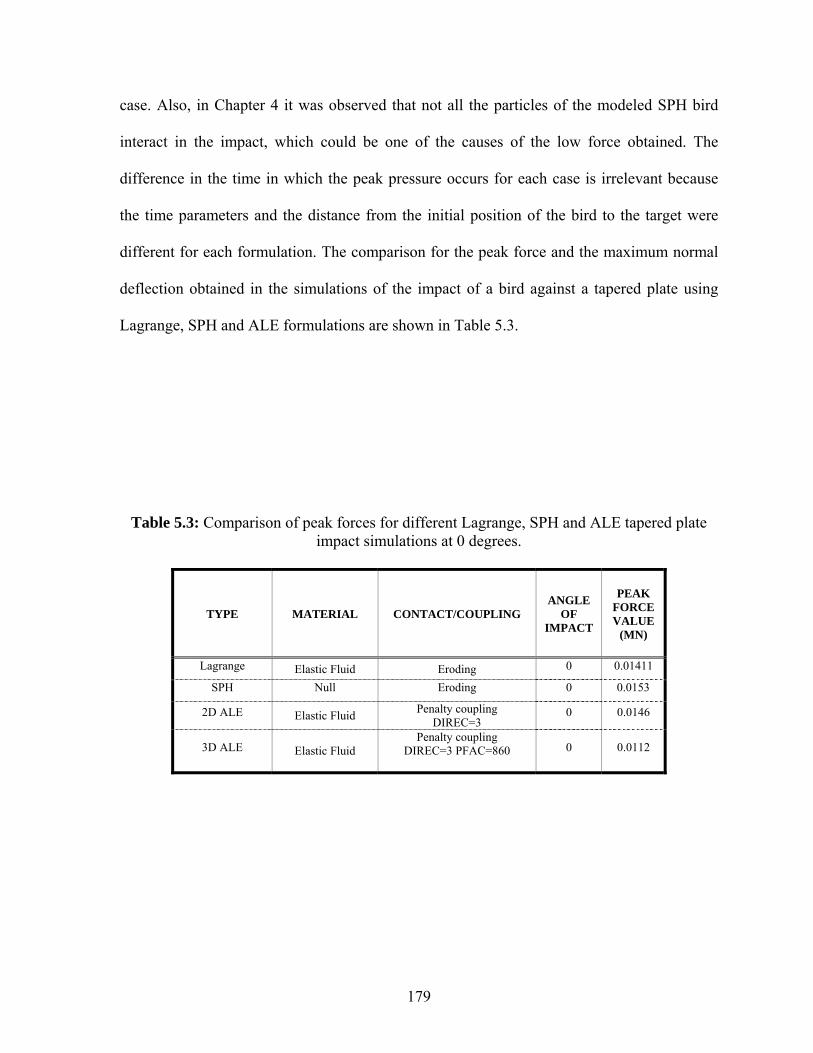
179
case. Also, in Chapter 4 it was observed that not all the particles of the modeled SPH bird
interact in the impact, which could be one of the causes of the low force obtained. The
difference in the time in which the peak pressure occurs for each case is irrelevant because
the time parameters and the distance from the initial position of the bird to the target were
different for each formulation. The comparison for the peak force and the maximum normal
deflection obtained in the simulations of the impact of a bird against a tapered plate using
Lagrange, SPH and ALE formulations are shown in Table 5.3.
Table 5.3: Comparison of peak forces for different Lagrange, SPH and ALE tapered plate
impact simulations at 0 degrees.
TYPE MATERIAL CONTACT/COUPLING ANGLE
OF IMPACT
PEAK FORCE VALUE
(MN)
Lagrange Elastic Fluid Eroding 0 0.01411 SPH Null Eroding 0 0.0153
2D ALE Elastic Fluid Penalty coupling DIREC=3
0 0.0146
3D ALE Elastic Fluid Penalty coupling
DIREC=3 PFAC=860
0 0.0112

180
Table 5.4: Comparison of peak forces for different Lagrange, SPH and ALE tapered plate impact simulations at 30 degrees.
TYPE
Material
CONTACT/COUPLING ANGLE
OF IMPACT
Maximum Normal
Deflection (in)
Error % from
Moffat
PEAK FORCE VALUE
(MN)
Moffat et al (2001) N/A N/A 30 1.05 N/A N/A
Lagrangian Elastic Fluid Eroding 30 1.19 13.38 0.0566
SPH Null Eroding 26,000 PARTICLES
30 1.12 6.96 0.0489
2D ALE Elastic Fluid PENALTY COUPLING 30 1.18 11.96 0.0532
3D ALE Elastic Fluid PENALTY COUPLING 30 1.25 19.8 0.0476

181
Chapter 6. Concluding Remarks
6.1 Conclusions
The three computational methods (Lagrangian, SPH and ALE) used in LS-DYNA
have shown to be robust for the one-dimensional beam centered impact problem. The peak
pressure from all three cases has an error smaller than 7% when compared to the analytical
results. For the Lagrangian and SPH the error is less than 5%. Thus, the three methods can be
used to study soft-body impact problems, such as bird-strike events.
For the frontal bird-strike impact against a flat rigid plate, the best contact was the eroding
contact type and the best Lagrangian material was material elastic fluid, which is a material
specialized to model a fluid-like behavior taking in consideration the deviatoric stresses
which are not considered for the null material. The Lagrangian simulations show that the
results are in within 10% when compared to already available experimental data in the
literature. The 2D ALE simulation, using an automatic mesh motion following a mass
weighted average velocity and a penalty coupling produced a peak pressure of 36 MPa, and
the results where within 10% with the pressure measured by Barber et al. (1975). The peak
pressure using the 3D ALE simulations showed sensibility to the time-step scale factor
(TSSFAC). It was shown that the best time scaled parameter is that of TSSFAC=0.58 which
produces an error of 12.12% when compared with that by Barber et al. (1975). Both
Lagrangian and ALE models used the material elastic fluid which can explain the
convergence in their results. For flat plate impact simulation using a SPH bird constructed

182
using two different mesh resolutions, if the contact *CONTACT_
CONSTRAINT_NODE_TO_SURFACE the pressure obtained is 37.3 MPa with an error of
6.75 % over the test data. Therefore, it is recommended to use the above type of contact
when studying SPH bird-strike events against rigid flat plate impacts simulations because it
better represents the deformations and pressure obtained with the test data.
For the 0 degree bird impact against a tapered plate, there was a small fluid-structure
interaction because the bird is basically sliced in two parts. This behavior is observed by all
three approaches.
For the 30 degrees bird impact against a tapered plate, the Lagrangian and SPH produce
peak forces within 10% error and the maximum normal deflection are found within 13.3%
when compared to the maximum normal deflection found by Moffat. However, the
maximum normal deflection found in this ALE simulation was 1.25 in, 19.73% higher than
the value found by Moffat et al. (2001). Therefore, based on these simulations the ALE
approach can be used for bird-strike events in tapered plates.

183
6.2 Recommendations for Future work
Further work in ALE bird-strike simulation for three dimensional cases should be
performed oriented to obtain a better deformation of the bird in the impact. For a 3
dimensional model of a bird strike, a study of the variables involved in the
*CONSTRAINT_LAGRANGE_IN_SOLID card need to be developed in order to set the
best combination of variables that produce a valid interaction between the Lagrangian and
the ALE parts of the model.
It is recommended the use of new versions of the ETA Femb PC Pre-Processor of LS-DYNA
or alternates software to create the models. This due to the fact that some of the features of
the version 28.0 of the ETA Femb PC Pre-Processor does not work properly.
A statistical study of the peak forces and pressures generated in the impact has to be
performed in order to better compare the results obtained using the three method Lagrange,
SPH and ALE with the experimental data.

184
References
Barber, J. P., H. R. Taylor and J. S. Wilbeck (1975). “Characterization of Bird Impacts on a Rigid Plate: Part 1”. Technical report AFFDL-TR-75-5.
Belytschko, T., W. Kam Liu and B. Moran (2001). “Nonlinear Finite Elements for
Continua and Structures”. John Wiley and Sons Ltd., England. Bertke, R. S. and J. P. Barber (1979). “Impact Damage on Titanium Leading Edges from
Small Soft Body Objects”. University of Dayton Research Institute for the Air Force Fligth Dynamics Laboratory, Wright-Patterson Air Force Base, OH. Technical Report AFML-TR-79-4019.
Birnbaum, N., N. Francis and B. Gerber (1997). “Coupled Techniques for the Simulation
of Fluid-Structure and Impact Problems”, Century Dynamics Inc. Bowman, D. R., G. J. Frank (2004). “IBRG ARTIFICIAL BIRD PROJECT”, Work
programmed and Schedule. Budgey, R. (2000). “The Development of a Substitute Artificial Bird by the International
Birdstrike Research Group for Use in Aircraft Component Testing”. Birdstrike Avoidance Team, Central Laboratory, Sand Hutton.
CAD-FEM (1999). “LS-DYNA – The Software for Large Deformation Dynamic
Analysis”, LS-DYNA News, Issue 3.
Carney, K., C. Lawrence, and D. Carney (2002). “Aircraft Engine Blade-Out Dynamics”. Proceedings of the 7th International LS-DYNA Users Conference. Session 14-3.
Cassenti, B. N. (1979). “Hugoniot Pressure Loading in Soft Body Impacts”. United
Technologies Research Center, Connecticut. Computational Fluid Dynamics: Smoothed Particle Hydrodynamics-Mathematical
(2002). Commonwealth Scientific & Industrial Research Organisation (CSIRO), Basis. http://www.cmis.csiro.au/CFD/sph/sph_math.htm
Donea, J., A. Huerta, J. Ponthot, and A. Rodríguez-Ferran (2004). “Arbitrary Lagrangian-
Eulerian Methods”. Encyclopedia of Computational Mechanics, Volume 1, Chapter 14.
eta/FEMB PC: User’s Manual (2001). Version 27. Livermore Software Technology
Corporation.

185
eta/FEMB PC: Training Manual (2001). Version 27. Livermore Software Technology
Corporation. Fung Y. (1994). “A FIRST COURSE IN CONTINUUM MECHANICS for Physical and
Biological Engineers and Scientists”. Prentice Hall, Englewood Cliffs, New Jersey. Getting Started with LS-DYNA (2002). Livermore Software Technology Corporation.
Goldsmith, W. (2001). “IMPACT: The Theory and Phisical Behaviour of Colliding Solids ”. Dover Publications, Mineola, New York.
Goyal, V. K., C. A. Huertas, T. R. Leutwiler and J. R. Borrero (2006a), “Robust Bird-
Strike Modeling Based On SPH Formulation Using LS-DYNA”, Proceeding of the 47th AIAA/ASME/ASCE/AHS/ASC Structures, Structural Dynamics & Materials Conference in Newport, Rhode Island. April 30 to May 4, 2006.
Goyal, V. K., C. A. Huertas, J. R. Borrero and T. R. Leutwiler (2006b), “Robust Bird-
Strike Modeling Based On ALE Formulation Using LS-DYNA”, Proceeding of the 47th AIAA/ASME/ASCE/AHS/ASC Structures, Structural Dynamics & Materials Conference in Newport, Rhode Island. April 30 to May 4, 2006.
Goyal, V. K. and C. A. Huertas (2006c), “Robust Bird-Strike Modeling Using LS-
DYNA”, Proceeding of the 23th Southeastern Conference on Theoretical and Applied Mechanics Conference in Mayagüez, PR. May 21-23, 2006.
Hallquist, J. (1998), LS-DYNA Theoretical Manual, Livermore Software Technology
Corporation. Hibbeler R. (1992). “Engineering Mechanics Statics and Dynamics”. Sixth Edition.
Macmillan Publishing company, New York.
Hut, P., L. Hernquist, G. Lake, J. Makino, S. McMillan and T. Sterling (1997) “Smooth
Particle Hydrodynamics: Models, Applications, and Enabling Technologies”,
Proceedings form the Workshop Presented by the Institute for Advance Study at
Princeton. June, 1997.
IBRG. (2004). “Artificial Bird Project - Work Programme and Schedule”. United
Kingdom.

186
LS-DYNA3D Interface, ICEM CFD Engineering, http://www-berkeley.ansys.com /interfaces/lsdyna3d.html
Karamchetti, K. (1980). “Principles of Ideal-Fluid Aerodynamics”. Krieger Publishing
Company, Florida. Lacome, J. (2001). “Smooth Particle Hydrodynamics-Part II, FEA Information
International News for the World-Wide Engineering Community”. November 2001, p. 6-11.
Lacome, J. (2000). “Smooth Particle Hydrodynamics (SPH): A New Feature in LS-
DYNA”. Proceedings of the 6th International LS-DYNA Users Conference. Session 7-3.
Linder, C. (2003). “An Arbitrary Lagrangian-Eulerian Finite Element Formulation for
Dynamics and Finite Strain Plasticity Models”. University Stuttgart, April, 2003. LS-DYNA Keyword User’s Manual (2003). Livermore Software Technology Corporation,
Version 970. LS-PRE/POST Manual (2002). Version 1.0. Livermore Software Technology
Corporation, The MacNeal-Schwendler Corporation (1996). “Bird Strike Simulation Using Lagrangian
& ALE Techniques with MSC/DYTRAN”, Presentation to United Technologies Corporation.
Martin N.F. (2004). “Nonlinear Finite Element Analysis to Predict Fan Blade Impact
Damage”, Pratt & Whitney. Melis, M. (2003). “Finite Element Simulation of a Space Shuttle Solid Rocket Booster Aft
Skirt Splashdown Using an Arbitrary Lagrangian-Eulerian Approach”. National Aeronautics and Space Administration (NASA), Glenn Research Center, Ohio, 2003.
Metrisin, J. and B. Potter (2001). “Simulating Bird Strike Damage in Jet Engines”.
ANSYS Solutions. Volume 3, Number 4. Pages 8-9. Moffat, T. J. and W. L. Cleghorn (2001). “Prediction of Bird Impact Pressures and
Damage using MSC/DYTRAN”. Proceedings of ASME TURBOEXPO 2001, Louisiana.
Monaghan, J. (1989). Journal of Computational Physics. May 1989.

187
Murat, B., S. K. Cing-Dao, E. B. Nabih, D. Ali and S. Ulku (2004). “Moving Beyond the
Finite Element, a Comparison Between the Finite Element Methods and Meshless Methods for a Ballistic Impact Simulation”, 8th International LS-DYNA Users Conference.
Niering, E. (1988). “Simulation of Bird Strikes on Turbine Engines ”, Turbinen-Union
Munich, Germany. Parkes, E. (1955). “The permanent deformation of a cantilever strucks transversely at its
tip”.Proc. Roy. Soc. Lond., England. Randall, P. P. (2003). “Smoothed-Particle-Hydrodynamics: The Search for Energy
Conservation”. Vassar College. Rosenblatt, M., G. E. Eggum, L. A. DeAngelo and K. N. Kreyenhagen (1976).
“Numerical Analyses of Soft Body Impacts on Rigid and Deformable Targets”. California Research and Technology, INC.
Serway, R. (1990). “PHYSICS: For Scientists & Engineers with Modern Physiscs”. Third
Edition. Saunders College Publishing, Philadelphia. Shultz, C. and J. Peters (2002). “Bird Strike Simulation Using ANSYS LS/DYNA”.
Phoenix Analysis and Design Technologies, Inc. Souli, M. and L. Olovsson (2000). “ALE and Fluid-Structure Interaction in LS-DYNA”.
Proceedings of the 6th International LS-DYNA Users Conference, Session 15-4. Stoker, C. (1999). “Developments of the Arbitrary Lagrangian-Eulerian Method in non-
linear Solid Mechanics”. HC Stoker Enschedel, The Netherlands. Stronge W.J. and T. Yu. (1993). “Dynamic Models for Structural Plasticity”. Springer-
Verlag, London, Great Britain. Tutt, B. and P. Taylor (2004). “The Use of LS-DYNA to Simulate the Water Landing of
Space Vehicles”. Proceedings of the 8th International LS-DYNA Users Conference.
Ubels, L.C., A.F. Johnson, J.P. Gallard and M. Sunaric (2003). “Design and Testing of a
Composite Bird Strike Resistant Leading Edge”. SAMPE Europe Conference
Exhibition, National Aerospace Laboratory.

188
Vasko, T. (2000). “Fan Blade Bird-Strike Analysis and Design”. Proceedings of the 6th International LS-DYNA Users Conference, Session 9-2.
Xue, L. (2004). “Breaking Dam Flood Using Smooth Particle Hydrodynamics Method”.
MIT University, May 2004.

189
Appendix A. LS-DYNA Overview
A.1 Features
LS-DYNA1 is a multifunctional finite element code used to model and analyze
deformations and dynamic response of structures and interactions between fluids and
structures. This software uses various finite element methods and explicit time integration to
predict the behavior of the object. LS-DYNA also has implicit capabilities; it can be used to
solve problems of structural analysis and heat transfer. The discretization of the finite
elements can be done using two-node beam elements, three- and four-node shell element,
eight-node solid elements and among other available elements within the code.
Some of the significant features in LS-DYNA are: full definition of contact areas, large
library of constitutive models, large library of element types and others. Beside these
features, there are different implicit solvers and capabilities for working with the Arbitrary
Lagrange Eulerian (ALE) method, Smooth Particle Hydrodynamics (SPH) thermal solver
and coupled fluid dynamics. These capabilities allow the user to solve different problems
with fluids and structures. Some of the main applications of LS-DYNA are crashworthiness,
metal forming, drop testing and bird-strike analysis.
1 Software developed by LSTC, Livermore Software Technology Corporation in California, USA.

190
LS-DYNA uses a KEYWORD INPUT database to define the characteristics of the model
and other important functions used in the simulation. One keyword can group many similar
functions. Each keyword is followed by a card input format to input the numerical values.
The keywords are described in the LS-DYNA Keyword User’s Manual (2003). To reset the
LS-DYNA default settings the Control keywords can be used. Other important keywords in
the LS-DYNS keyword input are the Material cards, Equation-of-state cards, the Element
cards, the Part definition cards, among others. The keyword input is written in data blocks
with the information pertaining to the keyword following it. The sign “*” must precede the
keyword and must be written in column one.
All of the keywords used in the software are presented in the Keyword User’s Manual with
explanations of the card input format for each keyword. One of the most important aspects of
the keyword input format is the relationship between the variables of the different keywords,
illustrated in Fig. 2.5. As it can be observed in the Fig. 2.5, the variables defined in the
*PART keyword are referenced in the following keywords (*SECTION, *MAT), if these
relationships are not defined carefully, an error could occur at the moment of the simulation.

191
*PART PID SID MID EOSID HGID
*SECTION_SHELL SID ELFORM SHRF NIP PROPT
*MAT_ELASTIC MID ρ E µ
*EOS EOSID
*ELEMENT EID PID NID
*NODE NID X Y Z
Figure 2.30: Illustration of keyword input relationships
Another tool for the data input is the ETA/FEMB PRE-PROCESSOR. This is a very useful
software within LS-DYNA, which allows model construction and the keyword input using a
graphical interface. With this software, the user is capable of creating the simulation in a user
friendly manner.
The tools used to plot results are the POST-GL version 1.0 and the LSTC PRE/POST
processor. These processors are also included within the LS-DYNA software and are used to
create three-dimensional plots of the deformation, stresses and strains that the models suffer
due to the impact. The LSTC PRE/POST also allows for the creation of graphs of the
maximum stresses and strains for the elements as a function of time.
192
A.2 Lagrangian Approach in LS-DYNA
In this section a description of a typical code for a Lagrangian simulation is
presented. The code is divided in sections depending on the function of each card. The first
section of the code is the *KEYWORD card and the function of this card is to let the
program know that the input of the data will be done in keyword format. Next is the *TITLE
card, this card is used to state the name of the simulation (it is optional).
The next section of the code involves the control cards for the execution of the simulation.
*CONTROL_TERMINATION: Mandatory and is used to specify the time of termination of
the program. With this card the user may specify the following variables.
ENDTIM : Termination time of the program,
ENDCYC : Termination cycle,
DTMIN : Reduction (scale) factor for the initial time step used to determine the
minimum time step.
ENDENG : Percent change in energy ratio for termination of calculations.
ENDMAS : Percent change in total mass for termination of calculation which is
only used if mass scaling is used to control the termination. For this
code, the only factor specified was the termination time.

193
*CONTROL_TIMESTEP: Used to control the time step for the calculations. In this card, the
user can specify the following variables:
DTINIT : Initial time step.
TSSFAC : Scale factor for computed time step. This variable will affect the time-
step as indicated in Eq. (B.1)
Nn tttTSSFACt ∆∆∆⋅=∆ + ,...,,min 21
1 (A.1)
Where, N is the number of elements. The time-step corresponds to the transient time
of an acoustic wave through an element using the shortest
characteristic distance.
ISDO : Basis of time size calculation for 4 node-shell elements, which is only
valid for shell elements.
DT2MS : Time step size for mass scaled solutions.
ERODE : Erosion flag for solid and t-shell elements when TSMIN in the
*CONTROL_TERMINATION card is reached. For the Lagrangian
models used in this work we used ERODE=1 which mean that erosion
is allowed.
The next section is that corresponding to the database controls for binary outputs. In this
section the software created output files are selected.

194
*DATABASE_BINARY_D3PLOT: Used to create a 3D plot of the simulation observed in
the Post-Processing software included in LS-DYNA.
DT : Time interval between outputs.
LCDT: Load curve ID. Specify time interval between dumps.
For the Lagrangian simulations performed, only the time interval between outputs
was specified.
For the output files also a section for database control for ASCII can be specified. In this
section.
*DATABASE_GLSTAT: Used to obtain global data of the system.
DT: Time interval between outputs
BINARY: Option to select what type of file will be created. For the BINARY
option, a “1” indicates that an ASCII file is written, a “2” indicates that a
binary database will be created and a “3” indicates that both files will be
created.
*DATABASE_RCFORC: This card was useful in this thesis. It is used to obtain the outputs
for the interacting forces in the contact of Lagrangian parts. It is necessary to indicate the
following variables:
DT: Time interval of output of the database
BINARY: Flag for binary output.

195
The code also provides a section to specify the parts, sections and material for the objects in
the simulation. This is done using the *PART, *SECTION and *MAT cards.
*PART: Used to identify each part and is related to the *SECTION and *MAT cards, since
the section and material ID are set by the user using this card. The *SECTION card is
followed by the type of element. As for example to define a shell element the
*SECTION_SHELL card is used. The *MAT card is used to specify the material properties
of each part. These cards may vary for each part only if each part has a different material or
the selected element is different.
In the *PART card, the user specifies the following values:
PID: Part ID.
SID: Section ID.
MID: Material ID.
EOSID: Equation of state defined in the *EOS card. This equation of state is
assigned to the material of the indicated in MID.
HGID : Hourglass identification.
Other options include the part initialization for gravity loading (GRAV) used for brick
elements and an option to identify thermal material property (TMID). The format of this card
is to identify the section ID (SID), which must be equal to the section ID defined in the
*PART card. For the *SECTION_SHELL card the user has to specify the element
formulation options (ELFORM), followed by the option to apply a shear correction factor
(SHRF) used to scale the transverse shear stress. The number of through thickness iteration

196
points (NIP) can be specified. Next the user can specify the quadrature or integration rule
(QR/IRID) followed by a card for composite materials (ICOMP). In the following line of this
card the user must input the thickness for each of the four elements that compose the shell
element (T1, T2, T3 and T4).
The material used in the Lagrangian simulations was the *MAT_NULL. This material allows
equation of state to be computed without computing deviatoric stresses. Erosion in tension
and compression is possible. When using the *MAT_NULL an equation of state, *EOS is
required. The *EOS_TABULATED card is used for the bird-strike simulation of this project.
MID: Material identification.
RO: Mass density.
PC: Pressure cutoff.
MU: Dynamic viscosity coefficient.
TEROD: Relative volume, V/Vo, for erosion in tension.
CEROD: Relative volume, V/Vo, for compression.
YM: Young modulus.
PR: Poisson’s ratio.
*EOS_TABULATED: A tabulated equation of state linearly dependent on the internal
energy.
EOSID: Indicates the characterizing number for the equation which is
referred in the corresponding part.
EV1, EV2 …EVN: Natural logarithm of the relative volume.
C1, C2 …C3: Constants.

197
T1, T2 …T3: Temperature constants.
GAMMA: γ
E0: Initial internal energy.
V0: Initial relative volume.
*SECTION_SOLID: Used to define section properties for the solid elements corresponding
to the bird. The type-1 element formulation corresponds to a constant stress solid
formulation. These section properties are assigned to the bird indicating the section ID in its
corresponding *PART card.
The ETA FEMB PC Preprocessor is used to edit some of the properties of the bird, renumber
the nodes of the blade and bird. The *SET_NODE_LIST also is used. The node ID gathered
in this node set list are those corresponding to the model of the bird. This set of nodes are
used to assign an initial velocity to the bird using the *INITIAL_VELOCITY card. A node
set can also be created to add constraint to the node set using the
*BOUNDARY_SPC_SET_ID card.
Next, the contact has to be defined between the bird and the blade. As an example of a
contact card, we chose the following contact type:
*CONTACT_SURFACE_TO_SURFACE_ID:
CID: Single number that identifies the contact.

198
SSID: Slave segment ID. Used to indicate the node ID, part ID, partset ID or
shell element ID that is going to slide in the master surface until a tensile
force develops.
MSID: Master segment ID. Indicates the master node ID, part ID, partset ID
or shell element ID.
SSTYP and MSTYP: Variables are used to indicate the type of entity to be
assigned to the slave segment and the master segment.
BT : Birth time in the third card input is set to zero which means that the
contact surface becomes active at time equal to zero.
DT : Default death time. The value in this card is set to 1.0e+20, which is
the time at when the contact surface is deactivated.
In the fourth card input, the scale factor for penalty stiffness for the slave and master
segments (SFS and SFM respectively) are set to one. In addition, the scale factors for the
slave and master surface thickness (SFST and SFMT respectively) have a value of one. The
Coulomb friction scale factor (FSF) and the viscous friction scale factor (VSF) are set also to
one.
When the material constants of the surfaces that are in contact have a wide variation of the
elastic bulk modulii, it may be necessary to use the soft constrain. When the value is zero, it
means that a penalty formulation is used.
The node information in the *NODE card corresponds to the nodes of the blade and the bird.
The nodes corresponding to the void were eliminated. As in the code showed for the ALE

199
simulation the elements are defined using the *ELEMENT_SHELL card for the blade part
corresponding to the blade and *ELEMENT_SOLID for the part corresponding to the bird.
A.3 ALE Approach in LS-DYNA
Souli and Olovsson (2000) mentioned four types of definitions for the ALE-mesh
motion:
1. Classical mesh smoothing
2. Motion following pre-defined load curves ahead of time
3. Automatic translation, rotation and stretching of elements in order to adapt to the
current location of the material inside the mesh.
4. Automatically translate and rotate the mesh, following a coordinate system defined by
three arbitrary nodes in the model.
The Pre-Defined Load Curve Motion as presented by Souli and Olovsson (2000) is presented
next. For this method, 12 load curves must be specified to solve for the velocities with the
Equation A.2:
i121110
987
654
3
2
1
ifffffffff
fff
⎪⎭
⎪⎬
⎫
⎪⎩
⎪⎨
⎧
⎥⎥⎥
⎦
⎤
⎢⎢⎢
⎣
⎡+
⎪⎭
⎪⎬
⎫
⎪⎩
⎪⎨
⎧=
⎪⎪⎭
⎪⎪⎬
⎫
⎪⎪⎩
⎪⎪⎨
⎧
z
yx
z
yx
(A.2)
In the above equation, fi(t) for i= 1,…,12 are the loads defined by the user. LS-DYNA uses
the keyword *ALE_REFERENCE_SYSTEM_CURVE to define the motion and deformation

200
for a geometric entity. This keyword allows the user to enter the 12 load curves described
above.
If the description of the motion of the material is unknown then the automatic motion can be
used. Souli and Olovsson (2000) described the rigid body translation defining the nodal
velocity as:
∑
∑
=
= ⎪⎭
⎪⎬
⎫
⎪⎩
⎪⎨
⎧
=⎪⎭
⎪⎬
⎫
⎪⎩
⎪⎨
⎧
N
1nn
N
1nn
m
mwvu
z
yx
c
c
c
(A.3)
where mn for n= 1,..,N are the nodal masses in the ALE mesh , n)w,v,u( are the nodal mass
flow velocities. The center of gravity of the ALE mesh is defined as:
∑
∑
=
= ⎪⎭
⎪⎬
⎫
⎪⎩
⎪⎨
⎧
=⎪⎭
⎪⎬
⎫
⎪⎩
⎪⎨
⎧= N
1nN
i
N
1nn
c
c
c
c
m
zyx
m
zyx
x
(A.4)
The node velocity can be written as:
⎪⎭
⎪⎬
⎫
⎪⎩
⎪⎨
⎧
−
−
−
⎥⎥⎥
⎦
⎤
⎢⎢⎢
⎣
⎡
−−
−
+⎪⎭
⎪⎬
⎫
⎪⎩
⎪⎨
⎧=
ci
ci
ci
xy
xz
yz
c
c
c
i
yzyyxx
zy
x
zyx
X'
'
'
ϖϖϖϖ
ϖϖ
(A.5)

201
LS-DYNA includes many commands or keywords implemented for the use of the ALE
simulation. For example, the *ALE_REFERENCE_SYSTEM_GROUP defines the type of
reference system for any part, element or other geometric entity. A geometric entity may be
moved, smoothed, expanded according to the reference system type defined. With the
*CONTROL_ALE card, the user can set default control parameters for the ALE and Eulerian
calculations. The velocity boundary conditions are defined automatically when using this
option.
The following capabilities for ALE and Eulerian formulations are available in LS-DYNA:
several smoothing algorithms, multi-material Eulerian elements, first and second order
advection methods, void materials, automatic slip, stick or silent boundary conditions for the
Eulerian simulations, acoustic pressure formulation, automatic to Lagrangian shell, brick or
beam element. Also it is possible to input Eulerian-Lagrangian coupling in LS-DYNA. This
could be done by defining two lists of Lagrangian and Eulerian materials coupled together.
This coupling method has many industrial applications.
A.3.2 Code explanation
Here we provide a brief description of the keywords used for a typical ALE
simulation in LS-DYNA. There some similarities with the Lagrangian formulation. The ALE
code is divided in different sections following the functionality of the card for a better
description. The following cards are same as for the Lagrangian description:
*KEYWORD
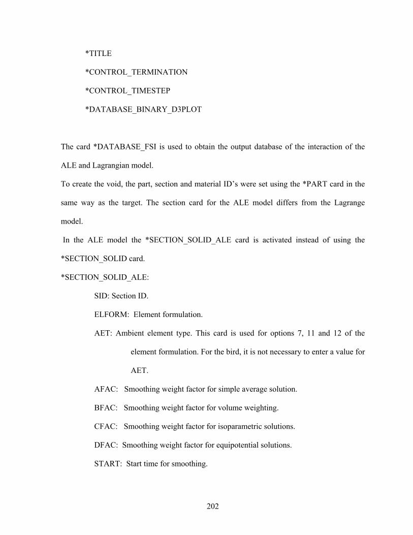
202
*TITLE
*CONTROL_TERMINATION
*CONTROL_TIMESTEP
*DATABASE_BINARY_D3PLOT
The card *DATABASE_FSI is used to obtain the output database of the interaction of the
ALE and Lagrangian model.
To create the void, the part, section and material ID’s were set using the *PART card in the
same way as the target. The section card for the ALE model differs from the Lagrange
model.
In the ALE model the *SECTION_SOLID_ALE card is activated instead of using the
*SECTION_SOLID card.
*SECTION_SOLID_ALE:
SID: Section ID.
ELFORM: Element formulation.
AET: Ambient element type. This card is used for options 7, 11 and 12 of the
element formulation. For the bird, it is not necessary to enter a value for
AET.
AFAC: Smoothing weight factor for simple average solution.
BFAC: Smoothing weight factor for volume weighting.
CFAC: Smoothing weight factor for isoparametric solutions.
DFAC: Smoothing weight factor for equipotential solutions.
START: Start time for smoothing.

203
END: End time for smoothing.
AAFAC: ALE advection factor. The smoothing weight factors are different
algorithms used to calculate the solution for the desired simulation.
The material for the void is defined using the *MAT_ELASTIC_FLUID. For this we define
the following values.
MID: Material ID.
RO: Density.
E: Modulus of elasticity.
PR: Poisson’s ration.
DA: Axial damping factor.
DB: Bending damping factor.
K: Bulk modulus.
VC: Tensor viscosity coefficient.
CP: Cavitation pressure.
The Bulk modulus, viscosity coefficient and the cavitation pressure are only defined for
fluids. In the example, since it was a fluid, the values of the modulus of elasticity, Poisson’s
ratio, and the damping factors were all zeroes.
*INITIAL_VOID_PART: Here the user defines the part ID for the part which is the void.
The *PART card was used to define the part ID of the target, the bird and the void mesh. The
section of the bird is defined using the *SECTION_SOLID_ALE (same as the void). The

204
material ID can also defined the same way as for the void, using the
*MAT_ELASTIC_FLUID.
In the section corresponding to the set part cards a list of the parts of the void and the bird are
grouped together using the keyword *SET_PART_LIST. This card is used to define a set of
parts with optional attributes. A unique number corresponding to the part set ID is used to
identify the set. It is necessary to indicate in the second card of the *SET_PART_LIST,
which parts are going to be grouped by indicating its corresponding part ID.
*ALE_REFERENCE_SYSTEM_GROUP: Used to define the type of reference system that
is being prescribed to a geometric entity (part, part set, node set, or segment set).
SID: Set ID. Corresponds to the same set defined before using the
*SET_PART_LIST card.
STYPE: The type of entity for the set ID is specified in the variable for the card
input format, the number “0” indicates that a part set is used.
PRTYPE: Defines the reference system type. The number “4” corresponds to an
automatic mesh motion following mass weighted average velocity in the
ALE mesh.
PRID: ID of switch list.
BCTRAN, BCEXP and BCROT: Used to set the translational, expansion and
rotation constraints for the ALE group the variables respectively are used.
The center of the mesh expansion XC, YC and ZC is the point (0, 0, 0).
205
EXPLIM: Limit ratio for mesh expansion in this work, defined with the variable, is
1.3.
*INITIAL_VELOCITY: Set the initial velocity for the grouped parts of the bird and the void
is set with the card. This card is used to define the nodal point initial translational velocities
using nodal set ID’s. The nodal set ID (NSID) is the same number assigned in the
*SET_NODE_LIST keyword, where all the nodes of the void mesh and bird material are
grouped.
*CONTROL_ALE: Sets the default control parameters for the arbitrary Lagrange-Eulerian
calculations.
DCT: Default continuum treatment. This was set to “2” which means an Eulerian
treatment. The method used for the advection is the Van Leer (VL) and the
Half-Index-Shift of second order (HIS).
*CONSTRAINED_LAGRANGE_IN_SOLID: Provide the mechanism for coupling
interaction between a slave Lagrangian geometric entity and a master ALE or Eulerian
geometry entity the keyword is used.
SSTYPE: In the variable of its card input the value of “1” indicates that the type of
the slave is a PID (Part ID), and then the indicated number for the slave
refers to the part which is the blade target shell. This part has to be a
Lagrangian part.
206
MSTYPE: The value of “0” indicates that the type of the master is a part set ID.
Then the number assigned to the MASTER variable corresponds to the
grouped ALE materials.
NQUAD: Cuadratule rule. The cuadrature rule states that there will be n×n coupling
points distributed over each Lagrangian segment surface (NQUAD=n).
CTYPE: Coupling type. If the coupling type is equal to four (CTYPE=4), then a
penalty coupling without erosion is used. The coupling direction is in normal
direction, compression only.
MCOUP: The variable has a value of “1” that means a coupling with material with
highest density.
PFAC: The penalty factor variable is set to zero. This value is used for scaling the
estimated stiffness of the interacting system and computes the coupling
forces to be distributed on the slave and master parts.
No friction is considered in the model (FRIC=0). By setting NORM=0, the normal vector
orientation of the Lagrangian shell part are defined according to the right hand rule.
Another section is that corresponding to the node set cards. In this section of the code the
nodes are grouped and the boundary nodes are specified. To group the nodes,
*SET_NODE_LIST card is used. For this card the set ID (SID) is specified, followed by
attributes that may be specified to the group (DA1, DA2, DA3, DA4). The next variables for
this card are the node ID’s (NID1, NID2… NID8) of the nodes to be grouped together.

207
*BOUNDARY_SPC_NODE: Add the required translational or rotational constraints to the
boundary nodes.
NID/NSID: The first variable is the node ID or nodal set ID. This specifies the
boundary nodes. The next variable is the coordinate system ID (CID).
Next, the translational and rotational constraints can be set for these
nodes by the user.
DOFX, DOFY and DOFZ: Set the translational constraints in the x, y and z
direction.
DOFRX, DOFRY and DOFRZ: Set The rotational constraints in the x, y and z axis.
The last section of the code describes the geometry and the list of the elements and nodes
used in the model. The coordinates for each node are given and the nodes are set in the
respective elements. The *NODE card define the nodes by their node ID (NID) and their x, y
and z coordinates. Also the user may set the translational constraints (TC) and the rotational
constraints (RC). With *ELEMENT_SOLID card the void mesh and the bird elements are
defined. It is required to identify the node ID and their respective part ID. First, the element
ID is set (EID), followed by the specification of the part ID (PID). Next, the nodes that
compose the element are specified. The element is an 8 node hexahedron, therefore for each
solid element 8-nodes must be specified (N1, N2… N8).
To define the element type for the blade target shell structure the *ELEMENT_SHELL
keyword is used. In this card the element ID (EID) must be set. Next the part ID (PID) is set.
208
This is a four node shell element and corresponds to the part ID (PID) “1”. For each shell
four nodes must be specified (N1, N2, N3, N4).
The last command of the code is the *END command which ends the simulation.
A.4 SPH Approach in LS-DYNA
For the Smooth Particle Hydrodynamics formulation, the initial particle masses,
densities, constitutive laws and coordinates must be set. All the particles of a neighborhood
need to have the same mass to make the particle mesh required regular enough. LS-DYNA
has implemented new keywords for the SPH elements used for explicit applications. Some
initials characteristics and properties for the SPH simulations have to be defined for the user.
The *CONTROL_SPH card is used to provide control parameters for computations
involving SPH particles. Some of the variables used in this keyword are: The number of
cycles between particle sorting, the BOXID that specified the box inside of which SPH
particles are computed, Death time, etc.
The *SECTION_SPH card is used to define the section properties for SPH particles. With
this keyword it is possible to define the constant applied to the smoothing length, the
minimum and maximum scale factor for the smoothing length, the initial smoothing length
and the start and stop time for the SPH approximation.

209
The *ELEMENT_SPH defines the particles in the nodes with its respective part ID and mass.
Although SPH is an extra layer of LS-DYNA, it is possible to use the other capabilities and
classical keywords of LS-DYNA.
It is necessary to use the SPH processor when there are SPH particles in the model. Some of
the material types available for SPH in the 970 version of LS-DYNA are:
*MAT_ELASTIC
*MAT_PLASTIC_KINEMATIC
*MAT_VISCOELASTIC
*MAT_HIGH_EXPLOSIVE_BURN
*MAT_NULL
*MAT_ELASTIC_PLASTIC_HYDRO
There is no need to define contact between SPH parts. This contact will only be defined
between two SPH materials when one particle of one material is inside the sphere of
influence of the other SPH material (Lacome, 2001). On the other hand, if there are any brick
or shell elements in the model, then it is necessary to use a NODE_TO_SURFACE contact.
The keywords *DATABASE_HISTORY_SPH and *DATABASE_SPHOUT generate a
SPHOUT file. The information carried for this file includes the stress variables such as
pressure, stresses, Von Misses and the strain variables

210
A.4.1 SPH code explanation A description of a typical SPH code for the bird-strike event simulation is now
presented. The first keyword in the code is the *KEYWORD card, used to inform the
program what will be the input. Next, the *TITLE card is used to input the title of the
simulation. The next section of the code is the control section. The *CONTROL_
TERMINATION keyword defines the termination time for the simulation. Also, the
termination may be specified for a cycle by specifying the ENDCYC variable. The
*CONTROL_TIMESTEP card is used to specify initial time step controls. The next control
keyword used is the *CONTROL_SHELL card, used to control calculations for the shell
elements. This keyword was used in this simulation to set the shell theory. The
*CONTROL_ENERGY card was used to apply the Stonewall Energy dissipation option.
Other controls that may be applied with this card are the Hourglass energy calculation, the
Sliding interface energy dissipation and the Rayleigh energy dissipation option.
The *CONTROL_SPH card is used to specify controls for the SPH calculations. The number
of cycles between particle sorting can be specified with the NCBS variable. The BOXID
variable is used to specify a box within the SPH computations will be done; no computations
will be made to the particles that move outside the specified box. The DT variable is used to
specify the “Death time”, which is the time when the SPH calculations will be stopped. The
IDIM variable is used to specify the dimensions of the problem (2D or 3D). The MEMORY
variable is used to set the number of neighboring particles for the initial calculation. The
FORM variable is used to input the particle approximation theory used. If a “0” is the input,
the default theory will be used, if a “1” is the input, the renormalization approximation will

211
be used. The start variable is used to input the time when the SPH particle approximations
will begin. The MAXV variable is used to identify the maximum velocity permitted for the
particles, particles that have a higher velocity will be deactivated. For this simulation the
values for the SPH controls were left as the default values.
The *DATABASE_BINARY_D3PLOT was used to specify the time for the time interval
between the output to the database. This was set with the DT/CYCL variable. The next
section of the code consisted of setting the parts, material and element definitions. The
*MAT_PIECEWISE_LINEAR_PLASTICITY card was used to define the material
properties for the target. The *MAT_PLASTIC_KINEMATIC card was used to define the
material properties for the beam. The *EOS_GRUNEISEN was used to define the equation
of state to be used for the calculations. The values for the variables used in this equation of
state must be set by the user for this command to work properly. The next card used was the
*SECTION_SPH used to define section properties for the SPH particles. The first variable
(SID) is used to set the section ID, followed by the CSLH variable that is used to set the
constant applied for the smoothing length of the particles.
The *PART commands are used to define the type of elements and material properties that
are applied to the parts used in the simulation. The material and element type are set using
the keywords explained before, they are applied to the respective parts by input of the section
ID (SID) and the material ID (MID) specified in the *MAT and *SECTION keywords.
212
The next keyword was the *NODE card used to input the ID and coordinates for each node.
The *ELEMENT_SOLID keyword was used to specify the nodes that composed the target,
which was a solid element composed of nodes 1 thru 8. Also in this card, the user specifies
the part ID for the solid element as defined in the *PART card. The *DEFINE_BOX
keyword was used to define a box that included all the SPH particles. This box was used as a
reference for the next keyword which is the *RIGIDWALL_PLANAR card. This card was
used to define the contact between a rigid surface and the nodal points of the deforming
body. The BOXID variable was used to specify that the nodes inside the “box 1” were the
slave nodes to the rigid wall. The FRIC variable was set to a value of “1”, which indicates a
constraint of no sliding after contact.
The *SET_NODE_LIST_GENERATE card was used to create a set node list consisting of
all the nodes that compose the cylinder. This list is used as reference for the initialization of
the velocity.
The next keyword was the *INITIAL_VELOCITY card, used to apply the initial velocity to
the cylindrical beam. The node set ID 1 and the BOX ID 1 (defined above) were set as the
part at which the initial velocity was applied, the initial velocity was -100 in the z direction.
The *ELEMENT_SPH card was used to define the elements that compose the cylinder as a
lumped mass element (Smooth Particles). The variables used for this card are the NID to set
the node ID of the nodes that compose the element, the PID to define the part to which these
elements are assigned and MASS to set the mass value for each particle.

213
The *END card was then used to finish the code.

214
Appendix B. Keyword for the 3D Lagrangian Simulation KEYWORD FOR THE 3 DIMENSIONAL LAGRANGIAN SIMULATION OF A BIRD-STRIKE $---+----1----+----2----+----3----+----4----+----5----+----6----+----7----+----8 $ LS-DYNA(970) DECK WRITTEN BY : eta/FEMB-PC version 28.0 $ ENGINEER : CARLOS HUERTAS ORTECHO $ PROJECT : DEVELOPMENT OF ROBUST ANALYTICAL MODELS FOR BIRD STRIKE $ UNITS : IN, LB*SEC^2/IN, SEC, LB $ TIME : 06:09:56 PM $ DATE : Tuesday, October 11, 2005 $---+----1----+----2----+----3----+----4----+----5----+----6----+----7----+----8 *KEYWORD $---+----1----+----2----+----3----+----4----+----5----+----6----+----7----+----8 *TITLE Lagrange $---+----1----+----2----+----3----+----4----+----5----+----6----+----7----+----8 $ $ $ CONTROL CARD $ $ $ $---+----1----+----2----+----3----+----4----+----5----+----6----+----7----+----8 *CONTROL_HOURGLASS $ IHQ QH 2 0.14 *CONTROL_TERMINATION $ ENDTIM ENDCYC DTMIN ENDENG ENDMAS 0.00040 0 0.25 0.0 0.0 *CONTROL_TIMESTEP $ DTINIT TSSFAC ISDO TSLIMT DT2MS LCTM ERODE MS1ST 0.0 0.70 0 0.0 0.0 0 1 0 $ DT2MSF $---+----1----+----2----+----3----+----4----+----5----+----6----+----7----+----8 $ $ $ DATABASE CONTROL FOR ASCII $ $ $ $---+----1----+----2----+----3----+----4----+----5----+----6----+----7----+----8 *DATABASE_GLSTAT $ DT BINARY 0.0000030 1 *DATABASE_RCFORC $ DT BINARY 0.0000030 3 *DATABASE_NCFORC $ DT BINARY 0.0000030 3 *DATABASE_SPHOUT $ DT BINARY 0.0000030 3 *DATABASE_ELOUT $ DT BINARY 0.0000010
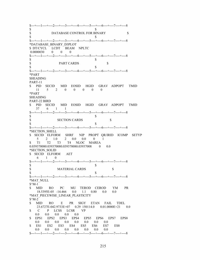
215
$---+----1----+----2----+----3----+----4----+----5----+----6----+----7----+----8 $ $ $ DATABASE CONTROL FOR BINARY $ $ $ $---+----1----+----2----+----3----+----4----+----5----+----6----+----7----+----8 *DATABASE_BINARY_D3PLOT $ DT/CYCL LCDT BEAM NPLTC 0.0000030 0 0 0 $---+----1----+----2----+----3----+----4----+----5----+----6----+----7----+----8 $ $ $ PART CARDS $ $ $ $---+----1----+----2----+----3----+----4----+----5----+----6----+----7----+----8 *PART $HEADING PART-11 $ PID SECID MID EOSID HGID GRAV ADPOPT TMID 11 5 2 0 0 0 0 0 *PART $HEADING PART-22 BIRD $ PID SECID MID EOSID HGID GRAV ADPOPT TMID 37 6 1 1 $---+----1----+----2----+----3----+----4----+----5----+----6----+----7----+----8 $ $ $ SECTION CARDS $ $ $ $---+----1----+----2----+----3----+----4----+----5----+----6----+----7----+----8 *SECTION_SHELL $ SECID ELFORM SHRF NIP PROPT QR/IRID ICOMP SETYP 5 2 1.0 2 0.0 0.0 0 1 $ T1 T2 T3 T4 NLOC MAREA 0.039370080.039370080.039370080.03937008 0 0.0 *SECTION_SOLID $ SECID ELFORM AET 6 1 0 $---+----1----+----2----+----3----+----4----+----5----+----6----+----7----+----8 $ $ $ MATERIAL CARDS $ $ $ $---+----1----+----2----+----3----+----4----+----5----+----6----+----7----+----8 *MAT_NULL $^M-1 $ MID RO PC MU TEROD CEROD YM PR 18.5395E-05 -14.466 0.0 1.1 0.80 0.0 0.0 *MAT_PIECEWISE_LINEAR_PLASTICITY $^M-2 $ MID RO E PR SIGY ETAN FAIL TDEL 23.6727E-042.9733E+07 0.29 150114.0 0.01.0000E+21 0.0 $ C P LCSS LCSR VP 0.0 0.0 0.0 0.0 0.0 $ EPS1 EPS2 EPS3 EPS4 EPS5 EPS6 EPS7 EPS8 0.0 0.0 0.0 0.0 0.0 0.0 0.0 0.0 $ ES1 ES2 ES3 ES4 ES5 ES6 ES7 ES8 0.0 0.0 0.0 0.0 0.0 0.0 0.0 0.0 $---+----1----+----2----+----3----+----4----+----5----+----6----+----7----+----8

216
$ $ $ EOS CARDS $ $ $ $---+----1----+----2----+----3----+----4----+----5----+----6----+----7----+----8 *EOS_TABULATED $^EQUATION_1 $ EOSID GAMA E0 V0 1 1.0 0.0 1.0 $ EV1 EV2 EV3 EV4 EV5 1.0 0.0 -0.0953 -0.1044 -0.1124 $ EV6 EV7 EV8 EV9 EV10 -0.1178 -0.1257 -0.1310001 -0.1483999 -0.2326999 $ C1 C2 C3 C4 C5 -5000.0 0.0 294.0 1470.0 2940.0 $ C6 C7 C8 C9 C10 4410.0 5880.0 7350.0 14700.0 73500.0 $ T1 T2 T3 T4 T5 0.0 0.0 0.0 0.0 0.0 $ T6 T7 T8 T9 T10 0.0 0.0 0.0 0.0 0.0 $---+----1----+----2----+----3----+----4----+----5----+----6----+----7----+----8 $ $ $ HOURGLASS CARDS $ $ $ $---+----1----+----2----+----3----+----4----+----5----+----6----+----7----+----8 *HOURGLASS $^HOURGLASS_1 $ HGID IHQ QM IBQ Q1 Q2 QB QW 1 2 0.14 0 1.5 0.060 0.0 0.0 $---+----1----+----2----+----3----+----4----+----5----+----6----+----7----+----8 $ $ $ NODE SET CARDS $ $ $ $---+----1----+----2----+----3----+----4----+----5----+----6----+----7----+----8 *SET_NODE_LIST $^NODE_SET 4 $ SID DA1 DA2 DA3 DA4 4 0.0 0.0 0.0 0.0 $ NID1 NID2 NID3 NID4 NID5 NID6 NID7 NID8 17522 17523 17524 17525 17526 17527 17528 17529 17531 17532 17533 17534 17535 17536 17537 17538 … 17280 17279 17278 17277 17260 17259 17258 17257 17256 *SET_NODE_LIST $^NODE_SET 5 $ SID DA1 DA2 DA3 DA4 5 0.0 0.0 0.0 0.0 $ NID1 NID2 NID3 NID4 NID5 NID6 NID7 NID8 35044 84278 84284 35050 34748 150569 150570 34754 … 81273 81272 81279 81278 81285 81284 81290 32056 81296 32062 32068 32038 32044 32050 32140 32146 32152 32158 32164

217
$---+----1----+----2----+----3----+----4----+----5----+----6----+----7----+----8 $ $ $ PART SET CARDS $ $ $ $---+----1----+----2----+----3----+----4----+----5----+----6----+----7----+----8 *SET_PART_LIST $^ $ SID DA1 DA2 DA3 DA4 1 0.0 0.0 0.0 0.0 $ PID1 PID2 PID3 PID4 PID5 PID6 PID7 PID8 37 $---+----1----+----2----+----3----+----4----+----5----+----6----+----7----+----8 $ $ $ BOUNDARY SPC CARDS $ $ $ $---+----1----+----2----+----3----+----4----+----5----+----6----+----7----+----8 *BOUNDARY_SPC_SET_ID $ ID 1 $ NSID CID DOFX DOFY DOFZ DOFRX DOFRY DOFRZ 4 0 1 1 1 1 1 1 $---+----1----+----2----+----3----+----4----+----5----+----6----+----7----+----8 $ $ $ INITIAL VELOCITY CARDS $ $ $ $---+----1----+----2----+----3----+----4----+----5----+----6----+----7----+----8 *INITIAL_VELOCITY $ NSID NSIDEX BOXID IRIGID 5 0 0 $ VX VY VZ VXR VYR VZR 0.0 0.0 -7795.276 0.0 0.0 0.0 $---+----1----+----2----+----3----+----4----+----5----+----6----+----7----+----8 $ $ $ CONTACT CARDS $ $ $ $---+----1----+----2----+----3----+----4----+----5----+----6----+----7----+----8 *CONTACT_ERODING_NODES_TO_SURFACE_ID $ CID 2 $ SSID MSID SSTYP MSTYP SBOXID MBOXID SPR MPR 5 11 4 3 1 1 1 $ FS FD DC VC VDC PENCHK BT DT 0.0 0.0 0.0 0.0 0.0 0 0.01.0000E+20 $ SFS SFM SST MST SFST SFMT FSF VSF 1.0 1.0 0.0 0.0 1.0 1.0 1.0 1.0 $ ISYM EROSOP IADJ 0 1 0 $ SOFT SOFSCL LCIDAB MAXPAR SBOPT DEPTH BSORT FRCFRQ 0 0.10 1.025 0.0 2.0 0 1 $ PENMAX THKOPT SHLTHK SNLOG ISYM I2D3D SLDTHK SLDSTF 0.0 0 0 0 0 0 0.0 0.0 $ IGAP IGNORE 2 0
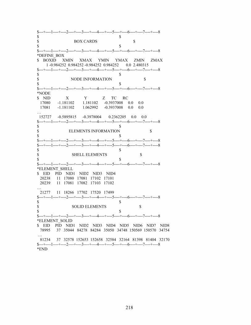
218
$---+----1----+----2----+----3----+----4----+----5----+----6----+----7----+----8 $ $ $ BOX CARDS $ $ $ $---+----1----+----2----+----3----+----4----+----5----+----6----+----7----+----8 *DEFINE_BOX $ BOXID XMIN XMAX YMIN YMAX ZMIN ZMAX 1 -0.984252 0.984252 -0.984252 0.984252 0.0 2.480315 $---+----1----+----2----+----3----+----4----+----5----+----6----+----7----+----8 $ $ $ NODE INFORMATION $ $ $ $---+----1----+----2----+----3----+----4----+----5----+----6----+----7----+----8 *NODE $ NID X Y Z TC RC 17080 -1.181102 1.181102 -0.3937008 0.0 0.0 17081 -1.181102 1.062992 -0.3937008 0.0 0.0 … 152727 -0.5895815 -0.3978004 0.2362205 0.0 0.0 $---+----1----+----2----+----3----+----4----+----5----+----6----+----7----+----8 $ $ $ ELEMENTS INFORMATION $ $ $ $---+----1----+----2----+----3----+----4----+----5----+----6----+----7----+----8 $---+----1----+----2----+----3----+----4----+----5----+----6----+----7----+----8 $ $ $ SHELL ELEMENTS $ $ $ $---+----1----+----2----+----3----+----4----+----5----+----6----+----7----+----8 *ELEMENT_SHELL $ EID PID NID1 NID2 NID3 NID4 20238 11 17080 17081 17102 17101 20239 11 17081 17082 17103 17102 … 21277 11 18266 17702 17520 17499 $---+----1----+----2----+----3----+----4----+----5----+----6----+----7----+----8 $ $ $ SOLID ELEMENTS $ $ $ $---+----1----+----2----+----3----+----4----+----5----+----6----+----7----+----8 *ELEMENT_SOLID $ EID PID NID1 NID2 NID3 NID4 NID5 NID6 NID7 NID8 78995 37 35044 84278 84284 35050 34748 150569 150570 34754 … 81234 37 32578 152653 152658 32584 32164 81398 81404 32170 $---+----1----+----2----+----3----+----4----+----5----+----6----+----7----+----8 *END

219
Appendix C. Keyword for the 2D ALE Simulation KEYWORD FOR THE 2 DIMENSIONAL ALE SIMULATION OF A BIRD-STRIKE $---+----1----+----2----+----3----+----4----+----5----+----6----+----7----+----8 $ LS-DYNA(970) DECK WRITTEN BY : eta/FEMB-PC version 28.0 $ ENGINEER : CARLOS HUERTAS ORTECHO $ PROJECT : DEVELOPMENT OF ROBUST ANALITYCAL MODELS FOR BIRD-STRIKE $ UNITS : MM, TON, SEC, N $ TIME : 07:23:08 PM $ DATE : Saturday, December 10, 2005 $---+----1----+----2----+----3----+----4----+----5----+----6----+----7----+----8 *KEYWORD 2000000 $---+----1----+----2----+----3----+----4----+----5----+----6----+----7----+----8 *TITLE LS-DYNA USER INPUT $---+----1----+----2----+----3----+----4----+----5----+----6----+----7----+----8 $ $ $ CONTROL CARD $ $ $ $---+----1----+----2----+----3----+----4----+----5----+----6----+----7----+----8 *CONTROL_ALE $ DCT NADV METH AFAC BFAC CFAC DFAC EFAC 2 1 2 -1.0 0.0 0.0 0.0 $ START END AAFAC VFACT PRIT EBC PREF NSIDEBC 0.0 0.0 0.0 0.000010 *CONTROL_ENERGY $ HGEN RWEN SLNTEN RYLEN 2 2 1 1 *CONTROL_TERMINATION $ ENDTIM ENDCYC DTMIN ENDENG ENDMAS 0.001 0 0.0 0.0 0.0 *CONTROL_TIMESTEP $ DTINIT TSSFAC ISDO TSLIMT DT2MS LCTM ERODE MS1ST 0.0 0.35 0 0.0 0.0 0 0 0 $ DT2MSF $---+----1----+----2----+----3----+----4----+----5----+----6----+----7----+----8 $ $ $ DATABASE CONTROL FOR ASCII $ $ $ $---+----1----+----2----+----3----+----4----+----5----+----6----+----7----+----8 *DATABASE_GLSTAT $ DT BINARY 0.0000072 1 *DATABASE_MATSUM $ DT BINARY 0.0000072 2
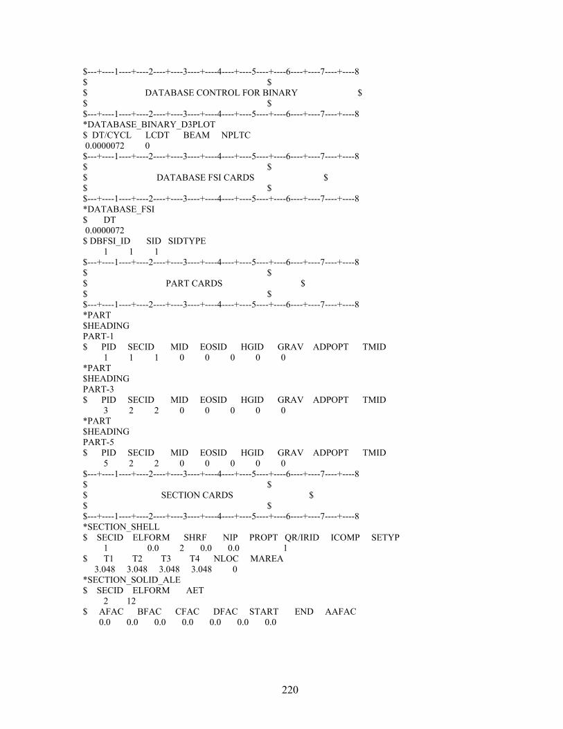
220
$---+----1----+----2----+----3----+----4----+----5----+----6----+----7----+----8 $ $ $ DATABASE CONTROL FOR BINARY $ $ $ $---+----1----+----2----+----3----+----4----+----5----+----6----+----7----+----8 *DATABASE_BINARY_D3PLOT $ DT/CYCL LCDT BEAM NPLTC 0.0000072 0 $---+----1----+----2----+----3----+----4----+----5----+----6----+----7----+----8 $ $ $ DATABASE FSI CARDS $ $ $ $---+----1----+----2----+----3----+----4----+----5----+----6----+----7----+----8 *DATABASE_FSI $ DT 0.0000072 $ DBFSI_ID SID SIDTYPE 1 1 1 $---+----1----+----2----+----3----+----4----+----5----+----6----+----7----+----8 $ $ $ PART CARDS $ $ $ $---+----1----+----2----+----3----+----4----+----5----+----6----+----7----+----8 *PART $HEADING PART-1 $ PID SECID MID EOSID HGID GRAV ADPOPT TMID 1 1 1 0 0 0 0 0 *PART $HEADING PART-3 $ PID SECID MID EOSID HGID GRAV ADPOPT TMID 3 2 2 0 0 0 0 0 *PART $HEADING PART-5 $ PID SECID MID EOSID HGID GRAV ADPOPT TMID 5 2 2 0 0 0 0 0 $---+----1----+----2----+----3----+----4----+----5----+----6----+----7----+----8 $ $ $ SECTION CARDS $ $ $ $---+----1----+----2----+----3----+----4----+----5----+----6----+----7----+----8 *SECTION_SHELL $ SECID ELFORM SHRF NIP PROPT QR/IRID ICOMP SETYP 1 0.0 2 0.0 0.0 1 $ T1 T2 T3 T4 NLOC MAREA 3.048 3.048 3.048 3.048 0 *SECTION_SOLID_ALE $ SECID ELFORM AET 2 12 $ AFAC BFAC CFAC DFAC START END AAFAC 0.0 0.0 0.0 0.0 0.0 0.0 0.0

221
$---+----1----+----2----+----3----+----4----+----5----+----6----+----7----+----8 $ $ $ MATERIAL CARDS $ $ $ $---+----1----+----2----+----3----+----4----+----5----+----6----+----7----+----8 *MAT_PLASTIC_KINEMATIC $^MAT PLASTIC KINEMATIC $ MID RO E PR SIGY ETAN BETA 13.9200E-09 205000.0 0.29 1035.0 0.99112 0.0 $ SRC SRP FS VP 0.0 0.0 0.0 0.0 *MAT_ELASTIC_FLUID $^MAT ELACTIC FLUID $ MID RO E PR DA DB K 29.1200E-10 23.94 0.0 0.0 0.0 2200.0 $ VC CP 0.30 239.4 $---+----1----+----2----+----3----+----4----+----5----+----6----+----7----+----8 $ $ $ NODE SET CARDS $ $ $ $---+----1----+----2----+----3----+----4----+----5----+----6----+----7----+----8 *SET_NODE_LIST $^NODE_SET 3 $ SID DA1 DA2 DA3 DA4 3 0.0 0.0 0.0 0.0 $ NID1 NID2 NID3 NID4 NID5 NID6 NID7 NID8 1 3 4 2 5 6 7 8 9 10 11 12 13 14 15 16 17 18 19 20 21 22 23 24 25 26 27 28 29 30 31 32 33 34 35 36 37 38 39 40 41 42 43 44 45 46 47 48 49 50 51 52 53 54 55 56 57 58 59 60 61 62 *SET_NODE_LIST $^NODE_SET 1 $ SID DA1 DA2 DA3 DA4 1 0.0 0.0 0.0 0.0 $ NID1 NID2 NID3 NID4 NID5 NID6 NID7 NID8 63 64 81 80 352 355 354 353 65 82 357 356 66 83 359 358 663 698 664 699 667 702 668 703 669 704 *SET_NODE_LIST $^NODE_SET 2 $ SID DA1 DA2 DA3 DA4 2 0.0 0.0 0.0 0.0 $ NID1 NID2 NID3 NID4 NID5 NID6 NID7 NID8 63 64 81 80 352 355 354 353 663 698 664 699 667 702 668 703 669 704 $---+----1----+----2----+----3----+----4----+----5----+----6----+----7----+----8 $ $
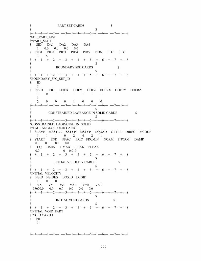
222
$ PART SET CARDS $ $ $ $---+----1----+----2----+----3----+----4----+----5----+----6----+----7----+----8 *SET_PART_LIST $^PART_SET 1 $ SID DA1 DA2 DA3 DA4 1 0.0 0.0 0.0 0.0 $ PID1 PID2 PID3 PID4 PID5 PID6 PID7 PID8 3 5 $---+----1----+----2----+----3----+----4----+----5----+----6----+----7----+----8 $ $ $ BOUNDARY SPC CARDS $ $ $ $---+----1----+----2----+----3----+----4----+----5----+----6----+----7----+----8 *BOUNDARY_SPC_SET_ID $ ID 2 $ NSID CID DOFX DOFY DOFZ DOFRX DOFRY DOFRZ 3 0 1 1 1 1 1 1 1 2 0 0 0 1 0 0 0 $---+----1----+----2----+----3----+----4----+----5----+----6----+----7----+----8 $ $ $ CONSTRAINED LAGRANGE IN SOLID CARDS $ $ $ $---+----1----+----2----+----3----+----4----+----5----+----6----+----7----+----8 *CONSTRAINED_LAGRANGE_IN_SOLID $^LAGRANGIAN SOLID CARD 1 $ SLAVE MASTER SSTYP MSTYP NQUAD CTYPE DIREC MCOUP 1 1 1 0 2 4 2 1 $ START END PFAC FRIC FRCMIN NORM PNORM DAMP 0.0 0.0 0.0 0.0 $ CQ HMIN HMAX ILEAK PLEAK 0.0 0 0.010 $---+----1----+----2----+----3----+----4----+----5----+----6----+----7----+----8 $ $ $ INITIAL VELOCITY CARDS $ $ $ $---+----1----+----2----+----3----+----4----+----5----+----6----+----7----+----8 *INITIAL_VELOCITY $ NSID NSIDEX BOXID IRIGID 1 0 0 $ VX VY VZ VXR VYR VZR 198000.0 0.0 0.0 0.0 0.0 0.0 $---+----1----+----2----+----3----+----4----+----5----+----6----+----7----+----8 $ $ $ INITIAL VOID CARDS $ $ $ $---+----1----+----2----+----3----+----4----+----5----+----6----+----7----+----8 *INITIAL_VOID_PART $^VOID CARD 1 $ PID 3 $---+----1----+----2----+----3----+----4----+----5----+----6----+----7----+----8

223
$ $ $ ALE CARDS $ $ $ $---+----1----+----2----+----3----+----4----+----5----+----6----+----7----+----8 *ALE_REFERENCE_SYSTEM_GROUP $^ALE_1 $ SID STYPE PRTYPE PRID BCTRAN BCEXP BCROT ICOORD 1 0 4 0 0 0 0 $ XC YC ZC EXPLIM 0.0 0.0 0.0 1.3 $---+----1----+----2----+----3----+----4----+----5----+----6----+----7----+----8 $ $ $ NODE INFORMATION $ $ $ $---+----1----+----2----+----3----+----4----+----5----+----6----+----7----+----8 *NODE $ NID X Y Z TC RC 1 0.0 150.0 -20.0 0.0 0.0 2 0.0 150.0 0.0 0.0 0.0 704 -76.23333 -10.0 -20.0 0.0 0.0 $---+----1----+----2----+----3----+----4----+----5----+----6----+----7----+----8 $ $ $ ELEMENTS INFORMATION $ $ $ $---+----1----+----2----+----3----+----4----+----5----+----6----+----7----+----8 $---+----1----+----2----+----3----+----4----+----5----+----6----+----7----+----8 $ $ $ SHELL ELEMENTS $ $ $ $---+----1----+----2----+----3----+----4----+----5----+----6----+----7----+----8 *ELEMENT_SHELL $ EID PID NID1 NID2 NID3 NID4 1 1 1 3 4 2 2 1 3 5 6 4 30 1 59 61 62 60 $---+----1----+----2----+----3----+----4----+----5----+----6----+----7----+----8 $ $ $ SOLID ELEMENTS $ $ $ $---+----1----+----2----+----3----+----4----+----5----+----6----+----7----+----8 *ELEMENT_SOLID $ EID PID NID1 NID2 NID3 NID4 NID5 NID6 NID7 NID8 287 3 63 64 81 80 352 355 354 353 288 3 64 65 82 81 355 357 356 354 590 5 669 243 260 259 704 532 549 548 $---+----1----+----2----+----3----+----4----+----5----+----6----+----7----+----8 *END